Embed Size (px)
Citation preview

Protoplanetary disk dynamics in highdust-to-gas ratio environments
Matıas Garate Silva
Munchen 2020


Protoplanetary disk dynamics in highdust-to-gas ratio environments
Matıas Garate Silva
Dissertation
an der Fakultat fur Physik
der Ludwig–Maximilians–Universitat
Munchen
vorgelegt von
Matıas Garate Silva
aus Santiago, Chile
Munchen, den 24.07.2020

Erstgutachter: Prof. Dr. Til Birnstiel
Zweitgutachter: Prof. Dr. Barbara Ercolano
Tag der mundlichen Prufung: 24.09.2020

Contents
Abstract xiii
1 Introduction 1
1.1 Evolution of a gas disk . . . . . . . . . . . . . . . . . . . . . . . . . . . . . 2
1.1.1 Viscous accretion . . . . . . . . . . . . . . . . . . . . . . . . . . . . 3
1.1.2 Photo-evaporation dispersal . . . . . . . . . . . . . . . . . . . . . . 5
1.1.3 Wind-Driven dispersal . . . . . . . . . . . . . . . . . . . . . . . . . 6
1.2 Gas orbital motion . . . . . . . . . . . . . . . . . . . . . . . . . . . . . . . 6
1.3 Dust dynamics . . . . . . . . . . . . . . . . . . . . . . . . . . . . . . . . . 7
1.3.1 Dust drifting and trapping . . . . . . . . . . . . . . . . . . . . . . . 9
1.3.2 Dust diffusivity . . . . . . . . . . . . . . . . . . . . . . . . . . . . . 9
1.3.3 Motivation for dust back-reaction. . . . . . . . . . . . . . . . . . . . 10
1.4 Dust growth . . . . . . . . . . . . . . . . . . . . . . . . . . . . . . . . . . . 10
1.5 Vertical structure . . . . . . . . . . . . . . . . . . . . . . . . . . . . . . . . 11
1.6 Paths to planet formation . . . . . . . . . . . . . . . . . . . . . . . . . . . 12
2 Coupled Gas and Dust Dynamics 15
2.1 Momentum Equations . . . . . . . . . . . . . . . . . . . . . . . . . . . . . 15
2.2 Back-Reaction Coefficients . . . . . . . . . . . . . . . . . . . . . . . . . . . 16
2.2.1 Single size approximation . . . . . . . . . . . . . . . . . . . . . . . 17
2.2.2 Correction for the dust diffusivity . . . . . . . . . . . . . . . . . . . 18
2.3 Accounting for the vertical structure . . . . . . . . . . . . . . . . . . . . . 18
2.4 Relevance of dust back-reaction . . . . . . . . . . . . . . . . . . . . . . . . 20
2.4.1 An analytical back-reaction condition . . . . . . . . . . . . . . . . . 20
2.4.2 Parameter space tests . . . . . . . . . . . . . . . . . . . . . . . . . 20
3 Effects of Dust Back-reaction in Disk Evolution 25
3.1 General setup in DustPy . . . . . . . . . . . . . . . . . . . . . . . . . . . . 25
3.2 Slowing viscous evolution . . . . . . . . . . . . . . . . . . . . . . . . . . . . 26
3.3 Dust accumulation at traffic jams . . . . . . . . . . . . . . . . . . . . . . . 28
3.4 Spreading of a dust ring . . . . . . . . . . . . . . . . . . . . . . . . . . . . 30
vi CONTENTS
4 An accretion event in RW Auriga? 374.1 Introduction . . . . . . . . . . . . . . . . . . . . . . . . . . . . . . . . . . . 37
4.1.1 Observations of RW Aur Dimmings . . . . . . . . . . . . . . . . . . 374.1.2 A Fast Mechanism for Dust Accretion . . . . . . . . . . . . . . . . 38
4.2 Model Description . . . . . . . . . . . . . . . . . . . . . . . . . . . . . . . 394.2.1 Dead Zone Model . . . . . . . . . . . . . . . . . . . . . . . . . . . . 394.2.2 Dead Zone Reactivation . . . . . . . . . . . . . . . . . . . . . . . . 41
4.3 Simulation Setup . . . . . . . . . . . . . . . . . . . . . . . . . . . . . . . . 414.3.1 Observational Constrains . . . . . . . . . . . . . . . . . . . . . . . . 414.3.2 Phase 1: Dust Concentration at the Dead Zone . . . . . . . . . . . 424.3.3 Phase 2: Dust Size Distribution at the Inner Disk . . . . . . . . . . 424.3.4 Phase 3: Dead Zone Reactivation . . . . . . . . . . . . . . . . . . . 444.3.5 Parameter Space . . . . . . . . . . . . . . . . . . . . . . . . . . . . 44
4.4 Dead Zone Reactivation Results . . . . . . . . . . . . . . . . . . . . . . . . 454.4.1 Simulation without Dust Concentration . . . . . . . . . . . . . . . . 484.4.2 Simulations for Different Dead Zone Properties . . . . . . . . . . . 504.4.3 Simulation with Dust Back-reaction . . . . . . . . . . . . . . . . . . 54
4.5 Discussion . . . . . . . . . . . . . . . . . . . . . . . . . . . . . . . . . . . . 564.5.1 The Fast Accretion Mechanism in the Context of RW Aur A Dimmings 564.5.2 A Single Reactivation Event, or Multiple Short Reactivation Spikes? 574.5.3 Validity of the Dead Zone Model . . . . . . . . . . . . . . . . . . . 58
4.6 Summary . . . . . . . . . . . . . . . . . . . . . . . . . . . . . . . . . . . . 59
5 Gas accretion damped by the dust back-reaction at the snowline 615.1 Introduction . . . . . . . . . . . . . . . . . . . . . . . . . . . . . . . . . . . 615.2 Model Description . . . . . . . . . . . . . . . . . . . . . . . . . . . . . . . 62
5.2.1 Evaporation and recondensation at the snowline . . . . . . . . . . . 625.3 Simulation Setup . . . . . . . . . . . . . . . . . . . . . . . . . . . . . . . . 63
5.3.1 Two-Population Dust Model . . . . . . . . . . . . . . . . . . . . . . 635.3.2 Disk Initial conditions . . . . . . . . . . . . . . . . . . . . . . . . . 645.3.3 Grid and Boundary Conditions . . . . . . . . . . . . . . . . . . . . 645.3.4 Parameter Space . . . . . . . . . . . . . . . . . . . . . . . . . . . . 65
5.4 Dust accumulation and gas depletion at the snowline . . . . . . . . . . . . 655.4.1 Accretion damped by the back-reaction . . . . . . . . . . . . . . . . 705.4.2 Depletion of H2 and He inside the snowline. . . . . . . . . . . . . . 725.4.3 What happens without the back-reaction? . . . . . . . . . . . . . . 735.4.4 The importance of the disk profile and size. . . . . . . . . . . . . . 73
5.5 Discussion . . . . . . . . . . . . . . . . . . . . . . . . . . . . . . . . . . . . 775.5.1 When is dust back-reaction important? . . . . . . . . . . . . . . . . 775.5.2 Other scenarios where the back-reaction might be important . . . . 785.5.3 Layered accretion by dust settling . . . . . . . . . . . . . . . . . . . 795.5.4 Observational Implications . . . . . . . . . . . . . . . . . . . . . . . 81
5.6 Summary . . . . . . . . . . . . . . . . . . . . . . . . . . . . . . . . . . . . 83

Contents vii
6 Distinguishing the origin of a dust ring. Photo-evaporation or planet? 856.1 Motivation . . . . . . . . . . . . . . . . . . . . . . . . . . . . . . . . . . . . 856.2 Implementation of photo-evaporation . . . . . . . . . . . . . . . . . . . . . 86
6.2.1 Gas loss rate . . . . . . . . . . . . . . . . . . . . . . . . . . . . . . 866.2.2 Dust loss rate . . . . . . . . . . . . . . . . . . . . . . . . . . . . . . 87
6.3 Implementation of a planet torque . . . . . . . . . . . . . . . . . . . . . . . 886.4 Early results . . . . . . . . . . . . . . . . . . . . . . . . . . . . . . . . . . . 89
6.4.1 Back-reaction effects on a planet induced ring. . . . . . . . . . . . . 896.4.2 Back-reaction effects on a photo-evaporation induced ring. . . . . . 916.4.3 Comparison between ring types . . . . . . . . . . . . . . . . . . . . 92
6.5 Caveats . . . . . . . . . . . . . . . . . . . . . . . . . . . . . . . . . . . . . 93
7 Conclusions and Outlook 97
A Derivation of the back-reaction coefficients 99A.1 System of linear equations . . . . . . . . . . . . . . . . . . . . . . . . . . . 99A.2 Solving for the dust velocities . . . . . . . . . . . . . . . . . . . . . . . . . 101A.3 Solving for the gas velocities . . . . . . . . . . . . . . . . . . . . . . . . . . 101
B Semi-Analytical test for back-reaction simulations 103B.1 An equivalent α value to describe the back-reaction. . . . . . . . . . . . . . 103
B.1.1 Setting up a test simulation . . . . . . . . . . . . . . . . . . . . . . 104B.1.2 Where the viscous approximation breaks . . . . . . . . . . . . . . . 106
C Gap opening criteria 107
Acknowledgements 118

viii Contents

List of Figures
2.1 Backreaction Study - Fiducial Model . . . . . . . . . . . . . . . . . . . . . 212.2 Backreaction Study - ε comparison . . . . . . . . . . . . . . . . . . . . . . 222.3 Backreaction Study - α comparison . . . . . . . . . . . . . . . . . . . . . . 232.4 Backreaction Study - vfrag comparison . . . . . . . . . . . . . . . . . . . . . 23
3.1 Numerical Applications - LBP Surface Density . . . . . . . . . . . . . . . . 273.2 Numerical Applications - LBP Dust Distribution . . . . . . . . . . . . . . . 283.3 Numerical Applications - LBP Accretion . . . . . . . . . . . . . . . . . . . 293.4 Numerical Applications - Traffic Jam Surface Density . . . . . . . . . . . . 303.5 Numerical Applications - Traffic Jam Dust Distribution . . . . . . . . . . . 313.6 Numerical Applications - Traffic Jam Accretion . . . . . . . . . . . . . . . 323.7 Numerical Applications - Dust Ring Density and Velocity . . . . . . . . . . 333.8 Numerical Applications - Dust Ring Density and Velocity . . . . . . . . . . 343.9 Numerical Applications - Dust Ring Size Distribution . . . . . . . . . . . . 35
4.1 Dead Zone Model . . . . . . . . . . . . . . . . . . . . . . . . . . . . . . . . 404.2 Surface Densities - Concentration Phase . . . . . . . . . . . . . . . . . . . 434.3 Dust Distribution - GrowthPhase . . . . . . . . . . . . . . . . . . . . . . . 444.4 Surface Density - Fiducial . . . . . . . . . . . . . . . . . . . . . . . . . . . 464.5 Dust Distribution - Fiducial . . . . . . . . . . . . . . . . . . . . . . . . . . 474.6 Accretion Rate - Fiducial . . . . . . . . . . . . . . . . . . . . . . . . . . . . 474.7 Comparison - Control . . . . . . . . . . . . . . . . . . . . . . . . . . . . . . 494.8 Comparison - CloseIn . . . . . . . . . . . . . . . . . . . . . . . . . . . . . . 514.9 Comparison - CloseOut . . . . . . . . . . . . . . . . . . . . . . . . . . . . . 524.10 Comparison - Shallow Dead Zone . . . . . . . . . . . . . . . . . . . . . . . 534.11 Comparison - Backreaction Effects . . . . . . . . . . . . . . . . . . . . . . 55
5.1 Stokes Number . . . . . . . . . . . . . . . . . . . . . . . . . . . . . . . . . 665.2 Surface density comparison . . . . . . . . . . . . . . . . . . . . . . . . . . . 675.3 Surface density evolution . . . . . . . . . . . . . . . . . . . . . . . . . . . . 685.4 Dust-to-gas ratio comparison . . . . . . . . . . . . . . . . . . . . . . . . . . 695.5 Gas velocity comparison . . . . . . . . . . . . . . . . . . . . . . . . . . . . 705.6 Accretion rate evolution . . . . . . . . . . . . . . . . . . . . . . . . . . . . 71

x List of Figures
5.7 Gas velocity decomposition . . . . . . . . . . . . . . . . . . . . . . . . . . . 715.8 H, He depletion comparison . . . . . . . . . . . . . . . . . . . . . . . . . . 725.9 Density Comparison - Backreaction . . . . . . . . . . . . . . . . . . . . . . 745.10 Dust-to-gas ratio comparison - Backreaction . . . . . . . . . . . . . . . . . 755.11 LBP surface density evolution . . . . . . . . . . . . . . . . . . . . . . . . . 765.12 LBP accretion rate evolution . . . . . . . . . . . . . . . . . . . . . . . . . . 775.13 Layered Accretion . . . . . . . . . . . . . . . . . . . . . . . . . . . . . . . . 80
6.1 Planet Ring - Backreaction Effects . . . . . . . . . . . . . . . . . . . . . . 906.2 Photo-evaporative Ring - Backreaction Effects . . . . . . . . . . . . . . . . 916.3 Ring Comparison . . . . . . . . . . . . . . . . . . . . . . . . . . . . . . . . 926.4 Multiple Ring Comparison . . . . . . . . . . . . . . . . . . . . . . . . . . . 95
B.1 Analytical test - Residual surface density . . . . . . . . . . . . . . . . . . . 105B.2 Analytical test - Accretion rate . . . . . . . . . . . . . . . . . . . . . . . . 105

List of Tables
2.1 Fiducial Parameters. Analytical Model. . . . . . . . . . . . . . . . . . . . . 21
3.1 Fiducial Parameters. Numerical Model. . . . . . . . . . . . . . . . . . . . . 263.2 Grid Parameters. Numerical Model. . . . . . . . . . . . . . . . . . . . . . . 26
4.1 Fiducial simulation parameters. . . . . . . . . . . . . . . . . . . . . . . . . 454.2 Parameter variations. . . . . . . . . . . . . . . . . . . . . . . . . . . . . . . 45
5.1 Parameter space. . . . . . . . . . . . . . . . . . . . . . . . . . . . . . . . . 65
6.1 Fiducial Parameters. Ring Models. . . . . . . . . . . . . . . . . . . . . . . 896.2 Grid Parameters. Ring Models. . . . . . . . . . . . . . . . . . . . . . . . . 90

xii List of Tables

Zusammenfassung
Protoplanetare Scheiben sind der Geburtsort von Planeten. Gas und Staub umkreisenden Zentralstern und unterliegen den Effekten der Schwerkraft, des Drucks, der Turbu-lenzen und der gegenseitigen Wechselwirkung. Mit dem Aufkommen neuer Teleskopebenotigen wir mehr denn je genaue Modelle zur Interpretation der Beobachtungen derScheiben, die eine Vielzahl von Unterstrukturen aufweisen. In dieser Arbeit untersuchenwir die Wirkung der gegenseitigen Wechselwirkung zwischen Gas und Staub auf die Dy-namik und Entwicklung protoplanetarer Scheiben, insbesondere in den Fallen, in denendas Staub-zu-Gas-Verhaltnis hoch genug ist, sodass die Festkorper dynamisch wichtigwerden. Wir leiten die kollektive Gas- und Staubdynamik aus den Impulserhaltungs-gleichungen her, indem wir die Wechselwirkung vom Staub auf die Gas-Reibung ein-beziehen und dabei den Beitrag mehrerer Staubarten berucksichtigen. Die resultieren-den Geschwindigkeiten werden in die Evolutions-Software Dustpy und Twopoppy imple-mentiert, welche die protoplanetaren Scheibe, die Advektion der Gas- und Staubkom-ponenten der protoplanetaren Scheibe zusammen mit dem Wachstum von Festkorperndurch Koagulation und Fragmentation losen. Schließlich kombinieren wir unsere Gle-ichungen fur die Fluiddynamik mit verschiedenen Scheibenszenarien, darunter die Reak-tivierung einer ”Dead Zone”, die Verdampfung und Kondensation von Wasser an derSchneegrenze und die Entwicklung einer Scheibe unter dem Einfluss von photoevapora-tionsgetriebenen Winden. Wir charakterisieren die Wirkung der Staubwechselwirkung aufdie Gas- und Staubdynamik in verschiedenen Szenarien. Wir stellen dabei fest, dass imFalle einer Dead-Zone-Reaktivierung der hohe Staubgehalt, der sich in den inneren Re-gionen ansammelt, die kollektive Scheibenentwicklung verlangsamt, da durch die gleicheviskose Kraft mehr Material abtransportiert werden muss. An der Schneegrenze kanndie Staubwechselwirkung den Gasstrom stoppen, die innere und außere Scheibe in Bezugauf den Gasfluss trennen und sowohl die radiale Ausdehnung als auch die Konzentra-tion der Staubansammlungen erhohen. Außerdem werden Staubringe, die sich am Randeiner photoevaporations-getriebenen Lucke bilden, uber eine großere Flache verteilt, da dieStaub-Ruckwirkung das Gasdruckprofil glattet, indem sie Material vom Druckmaximumwegdruckt. Zudem stellen wir fest, dass die Ruckreaktion die Scheibenentwicklung nur inUmgebungen mit hohen Staub-zu-Gas-Verhaltnissen, niedriger turbulenter Viskositat undbei großen Partikelgroßen merklich beeinflusst. Unsere Arbeit zeigt die Auswirkungen derStaub-Wechselwirkung auf die globale Scheibendynamik und kann verwendet werden, umBeobachtungssignaturen besser zu charakterisieren, indem ein genaueres Modell fur die

xiv Abstract
Staubverteilung sowie ein Leitfaden zur Beurteilung der Frage bereitgestellt wird, ob dieStaubwechselwirkung in der Scheibenentwicklung berucksichtigt werden sollte.

Abstract
Protoplanetary disks are the birthplace of planets. Gas and dust orbit around the centralstar subject to the forces of gravity, pressure, turbulence, and mutual drag. With theadvent of the new telescopes, we need more than ever accurate models to interpret theobservations of disks, which display a wide variety of substructures. In this work we studythe effect of the mutual drag force between gas and dust on protoplanetary disk dynamicsand evolution, particularly in the cases where the dust-to-gas ratio is high enough for thesolids to become dynamically important. We derive the collective gas and dust dynamicsfrom the momentum conservation equations, by including the back-reaction from the dustto the gas drag force, and considering the contribution of multiple dust species. The re-sulting velocities are implemented into the protoplanetary disk evolution codes Dustpy andTwopoppy, that solve the advection of the gas and dust components of the protoplanetarydisk, along with the growth of solids through coagulation and fragmentation. Finally, wecombine our equations for the fluid dynamics with different disk scenarios, including: there-activation of a dead zone, the evaporation and condensation of water at the snowline,and the evolution of a photo-evaporative disk. We characterize the effect of dust back-reaction on the gas and dust dynamics in the different scenarios. We find that in theevent of a dead zone re-activation the high dust content accumulated in the inner regionsdamps the collective disk motion, since more material is carried away by the same viscousforce. At the snowline the dust back-reaction can stop the gas flow, disconnect the innerand outer disk in terms of gas accretion, and enhance both the radial extend and thelevel concentration of dust accumulations. Also, dust rings formed at the edge of a photo-evaporative gap are spread over a wider area, since the dust back-reaction smooths the gaspressure profile by pushing the material away from the pressure maximum. Lastly, we findthat the back-reaction only affects the disk motion in environments with high dust-to-gasratios, low turbulent viscosity, and large particle sizes. Our work shows the effects of thethe dust back-reaction on the global disk dynamics, and can be used to better characterizeobservational signatures, by providing a more accurate model for the dust distribution, aswell as a guideline to assess whether the dust back-reaction should be considered, giventhe disk conditions.

xvi Abstract

Chapter 1
Introduction
In the last decade, with the advent of new telescopes and instruments, protoplanetary diskobservations have revolutionized our understanding of planet formation. We transitionedfrom having only spectral information and unresolved images, to high-angular resolutionimages of gas and dust in scattered-light, millimeter continuum, and narrow band-emission.The observations have revealed disks with multiple rings, gaps, and signposts of planetformation, which previously where only studied through theoretical models. Similarly,numerical models have grown more complex, allowing us to make testable predictionsabout these disks, and to explain the observed features.Studying the evolution of protoplanetary disks can help us to understand the diversity ofexoplanetary systems found in the recent decades, the process of planet formation, and thediversity of disk morphologies found since the first ALMA observation of HL Tau (ALMAPartnership et al., 2015; Ansdell et al., 2016; Andrews et al., 2018).Protoplanetary disks are born during the process of star formation. It all begins when acloud of gas and dust collapses due to its own gravity, resulting in a central star and thesurrounding envelope orbiting around it.As the envelope contracts, it also speeds up due to the conservation of angular momentum.The centrifugal force balances the radial component of the stellar gravity (when viewed incylindrical coordinates in the rotation frame of the material), while the vertical componentforces the material to settle towards the midplane, until the pressure support is strongenough to counter the stellar gravity.The evolution of protoplanetary disks lasts for approximately 10 Myr (Strom et al., 1989;Skrutskie et al., 1990; Haisch et al., 2001), and ends once all the material has been dispersed,accreted into the star, or transformed into planets and debris disks.The dynamic of disk is affected by several forces acting over the gas and dust component.These include the stellar gravity, the gas pressure, the viscous drag, the magnetic force,the radiation pressure, the torque exerted by a forming planet, and the drag force betweengas and dust, among others.In the classical disk evolution models the dust is assumed to be only a 1% of the total gasmass, as in the interstellar medium (ISM, Bohlin et al., 1978). Under this assumption, thedrag force exerted by the dust onto the gas is negligible for their collective evolution, and

2 1. Introduction
the gas component evolve independently of the solid grains. However, both observationsand theoretical models show that the dust grains can concentrate in different regions ofthe disk (Pinilla et al., 2012; ALMA Partnership et al., 2015), reaching higher dust-to-gasratios for which the dust back-reaction becomes dynamically important for the collectivegas and dust evolution.In this work we extend the traditional expressions for the gas and dust velocities, byincluding the contribution of the drag force back-reaction from the dust onto the gas, andstudy the disk evolution in high dust-to-gas ratio environments considering the collectivegas and dust dynamics.This thesis is structured as follows:In Chapter 1 we review the classical model of gas and dust evolution, where the dust back-reaction is typically ignored.In Chapter 2 we derive the correct expressions for the gas and dust velocities consideringthe dust back-reaction onto the gas, and analyse the new expressions.In Chapter 3 we perform numerical simulations of protoplanetary disks that illustrate theeffects of dust back-reaction.In Chapter 4 and 5 we study the disk evolution by considering respectively: the reactivationof a dead zone, the water snowline.In Chapter 6 we report our work in progress in the study case of dust accumulation arounda gap, opened either by photo-evaporation or by a massive planet.In Chapter 7 we summarize our work and propose future applications in which the collectivedynamics of gas and dust might be a key ingredient.
1.1 Evolution of a gas disk
Observations of young star forming regions reveal that protoplanetary disks are typicallyfound in systems younger than 10 Myrs (Haisch et al., 2001). During this time all thegas must be either accreted towards the star or blown away. Currently, we know of threemechanisms that can lead to disk dispersal: viscous accretion (Shakura & Sunyaev, 1973;Lynden-Bell & Pringle, 1974), photo-evaporation (Alexander et al., 2006a,b), and magneticdriven winds (Blandford & Payne, 1982). These processes work by either redistributingthe material across the disk, or by removing it into the interstellar medium.The mass transport of the gas disk can be modelled as a continuity equation:
∂
∂t(rΣg) +
∂
∂r(rΣg vg,r) = 0 (1.1)
where Σg is the gas surface density of the disk, r is the distance to the central star, andvg,r is the gas velocity in the radial direction.We use this advection equation in our disk evolution models, assuming axial symmetryand vertical hydro-static equilibrium. While this assumption is simple, it allows to incor-porate more ingredients in the models, and understand the basic principles that governthe disk evolution. Moreover, high angular resolution observations show that most disks

1.1 Evolution of a gas disk 3
are axisymmetric (see DSHARP observations, Andrews et al., 2018), despite presentingsubstructures.While this approximation is good in general, we should note that it will fail fail in sit-uations where the disk rotation deviate significantly from keplerian motion, such as inregions with steep pressure gradients, massive self-gravitating disks that present fragmen-tation (Lichtenberg & Schleicher, 2015), or disks with a massive companion that createsstrong perturbations, such as spirals or a tilted inner disk (Cuello et al., 2019a; Nealonet al., 2020).Now we proceed to describe each of the gas dispersal mechanisms, along with the equationsrelevant to our model.
1.1.1 Viscous accretion
Observations reveal that protoplanetary disks present a wide range of accretion rates ontothe star, with values ranging between 10−10 M/yr to 10−6 M/yr (Hartigan et al., 1995;Manara et al., 2017), varying with the age, mass, and morphology of the disk.To produce such accretion rates, there must exist an underlying process responsible oftransporting the material towards the star.In a keplerian disk orbiting around a star with mass M∗, the material orbits with an angularvelocity of:
ΩK =
√GM∗r3
, (1.2)
with G the gravitational constant.In such a disk, the exchange of material between two neighboring rings of gas results in theoutwards transport of angular momentum, causing the inner ring to spread inward whilethe outer ring spreads outwards. On global scales, this causes in the inner regions of thedisk to be accreted towards the star while the outer regions disperse outwards (Lynden-Bell& Pringle, 1974; Pringle, 1981).The efficiency of the angular momentum transport is controlled by the exchange of ma-terial between adjacent gas parcels. The observed disk lifetimes and the correspondingaccretion rates indicate that molecular diffusivity is too low to be the dominant driver ofdisk accretion. Turbulence, which transports material much faster, is a better candidate tofit the observational constraints, and can can be modeled as a viscous torque acting overthe fluid, which results in the gas evolving as a diffusive process (Lust, 1952; Lynden-Bell& Pringle, 1974):
∂Σg
∂t=
3
r
∂
∂r
(r1/2 ∂
∂r
(νΣgr
1/2))
, (1.3)
where ν is the viscosity of the material.The turbulent viscosity ν, can be written according to the α model (Shakura & Sunyaev,1973) as follows:
ν = α c2sΩ−1K , (1.4)

4 1. Introduction
where cs is the gas isothermal sound speed:
cs =
√kBT
µmH
, (1.5)
with kB the Boltzmann constant, T the gas temperature, µ the mean molecular weight,and mH the hydrogen mass.The dimensionless α parameter (with α < 1) controls the strength of the turbulent vis-cosity. Numerical models indicate that the α parameter has values between 10−4 to 10−1,depending on the physical process that drives the turbulence.Some of the instabilities that can stir the gas turbulence are the Magneto Rotational Insta-bility (MRI, Balbus & Hawley, 1991), the Vertical Shear Instability (VSI, Nelson et al.,2013; Stoll & Kley, 2014), and the Gravitational Instability (GI, Lin & Pringle, 1987),among others.The viscous evolution of the disk, written as a diffusive process in Equation 1.3, can alsobe expressed as an advection equation (1.1), with the following viscous velocity:
vν = − 3
Σg
√r
∂
∂r(ν Σg
√r). (1.6)
In terms of the momentum conservation equation, the force responsible for viscous diffusioncan be written as:
fν =1
2ΩKvν , (1.7)
where fν is the viscous force per mass unit in the azimuthal direction. We find that theexpression for the viscous velocity vν , and the viscous force fν are particularly useful tore-derive the gas velocity in presence of additional force terms, as we will do in Chapter 2.
Steady state solution
If the disk evolution is dominated by viscous accretion, then Equation 1.1 has a steadystate solution given by:
3πΣg ν = Mg
(1−
√rin
r
), (1.8)
with rin the disk inner boundary (where the torque is assumed to be zero), and the gasaccretion rate Mg being constant in time and radii. In the disk regions far from the inneredge (r rin), this solution can be simplified to:
3 πΣg ν = Mg, (1.9)
which implies that the gas surface density is inversely proportional to the viscosity ν insteady state. In particular, for a disk with α-viscosity, and a temperature profile of T ∝ r−q,the steady state gas surface density follows a power law profile:
Σg(r) = Σ0
(r
r0
)−p. (1.10)

1.1 Evolution of a gas disk 5
with Σ0 and r0 the normalization parameters, and p = 3/2 − q the power law exponent.For a characteristic irradiated disk the temperature profile presents a value of q = 0.5, andp = 1.Another consequence of the steady state solution is that regions with low turbulent viscosityact as a bottleneck for the gas accretion, accumulating more material than regions withhigher viscosity. Dead zones, which are regions with low turbulence due to an inefficientMRI (Gammie, 1996), show this behavior. As we see in Garate et al. (2019) (see alsoChapter 4), these regions also act as dust traps, and are an ideal scenario to study thecollective gas and dust dynamics.
Self similar solution
Another analytical solution to the advection equation has the form of a power law with anexponential cut-off:
Σg(r) = Σ0
(r
r0
)−1
exp(−r/rc), (1.11)
where Σ0 and r0 are the normalization values of the profile, and rc is the cut-off radius. Thisexpression assumes that the disk has an outer edge, while the power-law profile assumesthat the disk extends to infinity.The viscous evolution of this profile retains the same shape of Equation 1.11, while theparameters Σ0(t) and rc(t) change with time. Because of this property, this profile iscalled the self-similar solution (Lynden-Bell & Pringle, 1974). In Equation 1.11 we showthe particular solution valid for ν ∝ r (which is consistent disk with an α-viscosity profile,and a q = 0.5 temperature profile, Equation 1.4).
1.1.2 Photo-evaporation dispersal
Besides the viscous diffusion of material, the protoplanetary disk can also lose gas throughphoto-evaporative winds (Alexander et al., 2006a). This is the case when the radiationemitted by the central star (or neighboring stars) in the high energy range (Far UV,Extreme UV, and X-Ray) is intense enough to unbound the gas from the surface layers ofthe protoplanetary disk.The outer regions of the disk, where the material is loosely bound to the star, are moresusceptible to photo-evaporation than the inner regions. The gravitational radius, for whichthe thermal energy of the excited material exceeds the gravitational energy (Alexanderet al., 2006b), is given by:
rg =GM∗c2s
. (1.12)
This can be modeled as a loss term Σwind, that acts on the regions where r ≥ rg. Thisapproach assumes that only the angular momentum of the ejected material is removedfrom the disk, without accelerating the remaining material.A consequence of the mass loss through photo-evaporation is the opening of a gap at the

6 1. Introduction
gravitational radius, since the material in the inner regions continues to evolve throughviscous accretion, while the material in the outer regions is dispersed (Alexander et al.,2006a), disconnecting the inner and outer regions in terms of mass accretion, and leadingto an inside-out dispersal of the disk mass (Koepferl et al., 2013).After the cavity is opened, we expect to find different observational signatures. First, thedepletion of the inner regions should lead to a reduced NIR emission, characteristic of“transition disks” objects, though it is worth noting that photo-evaporation is not the onlymechanism that can lead to transition disk signatures. Planets, for example can also clearthe inner regions (for a review on transition disks, see Espaillat et al., 2014).Another consequence of the gap opening, is the creation of a pressure maximum in the gasand the outer boundary of the cavity. As we will see in the following sections, this regioncan become a dust trap, and present itself as a dust ring in the observations.
1.1.3 Wind-Driven dispersal
Another method that has been proposed to explain disk dispersal is the presence of mag-netic driven winds (Suzuki & Inutsuka, 2009). In a disk with a vertical magnetic fieldcomponent, the surface of the disk experiences an additional torque that can accelerateand launch the material away (Blandford & Payne, 1982). The escaped material carriespart of the disk angular momentum, which in turn, causes the remaining gas to drift in-wards.However, recent simulations show that the magnetic winds can only drive a minor fractionof the total angular momentum transport and the accretion rate onto the star, and there-fore would not contribute to the disk dispersal. (Zhu & Stone, 2018).From the reviews of Turner et al. (2014); Ercolano & Pascucci (2017) it seems that the neteffect of magnetic winds onto the disk evolution is not yet understood.For this reason, among others, we will leave this component of the disk evolution outsidethe scope of this work, as it is not clear what the interaction between magnetic winds anddust evolution might be.In the future, once we can determine a reliable mass loss rate profile, we extend our im-plementation of disk dispersal through photo-evaporation (see Chapter 6), by adjusting itto the magnetic winds mechanism.
1.2 Gas orbital motion
A test particle in a protoplanetary disk is subject to the stellar gravity and orbits the starat keplerian speed vK = ΩKr. However, a parcel of gas also experiences a pressure forcethat can aid or oppose the stellar gravity in the radial direction:
fP = − 1
ρg,0
∂P
∂r, (1.13)

1.3 Dust dynamics 7
where ρg,0 is the gas volume density at the midplane, P = ρg,0 c2s is the isothermal gas
pressure.Approximating to first order, the resulting difference between the keplerian velocity andthe gas orbital velocity is:
vP = −1
2
(hgr
)2∂ logP
∂ log rvK , (1.14)
where hg is the gas scale height given by:
hg = cs Ω−1K . (1.15)
Through this work we call vP the “pressure velocity”, though in the literature it can alsobe found as vP = ηvK (Nakagawa et al., 1986), with η the corresponding pre-factor fromEquation 1.14. For a smooth disk, the pressure gradient is negative, meaning that the gasorbits at sub-keplerian speed, however, if the disk presents any pressure maximum, theregions with positive pressure gradient will orbit at super-keplerian speed.Though the pressure velocity is only a small fraction of the keplerian orbital speed (typicallyvP ∼ 10−3vK), this difference dominates the drag force between gas and dust, as we willsee in the following sections.
1.3 Dust dynamics
The dust component of protoplanetary disks comes in a wide range of sizes, from micron-sized grains to millimeter pebbles. Near and far infrared observations from Spitzer, Herscheland other telescopes trace the hot emission from small particles, while interferometric ob-servations from ALMA reveal the structures made by large millimeter particles.Both theory and observations agree that the gas and dust components behave different,and that different particle species behave in a different manner. The observations of theTW Hya disk are a good example of how the line emission from the gas (Huang et al.,2018), the scattered-light from small micrometer dust grains (van Boekel et al., 2017), andthe continuum emission from millimeter large grains show a different radial extend, anddifferent sub-structures (Andrews et al., 2016). Observable quantities, like the spectralindex, also suggest that large grains drift towards the inner regions (Tazzari et al., 2016;Tripathi et al., 2018).Finally, observations of different types of sub-structures (spirals, gaps, etc) indicate under-lying dust and gas interactions (see section 5.3.1 of Andrews, 2020).The radial transport of dust particles across the disk can be modeled with a continuityequation, as in Equation 1.1, with the addition of a dust diffusivity term:
∂
∂t(rΣd(m)) +
∂
∂r(rΣd(m) vd,r(m))− ∂
∂r
(rDd(m)Σg
∂
∂r
(Σd(m)
Σg
))= 0, (1.16)
where Σd, vd,r, and Dd correspond to the surface density, radial velocity, and diffusivity ofa particular dust species of mass m.
8 1. Introduction
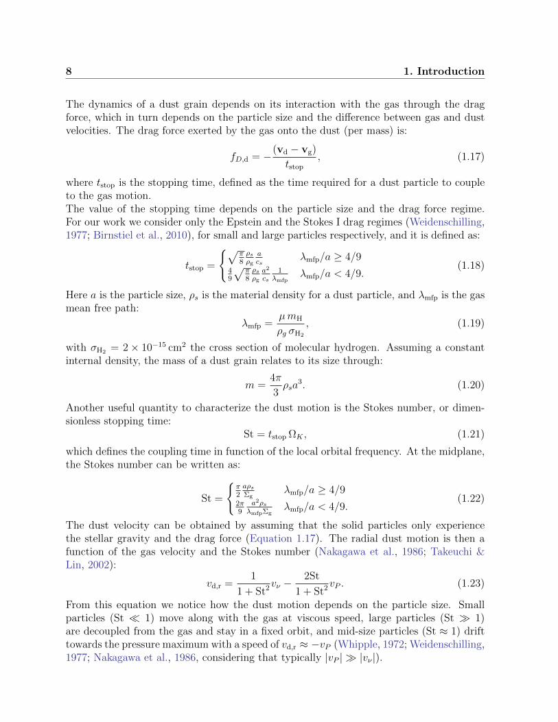
The dynamics of a dust grain depends on its interaction with the gas through the dragforce, which in turn depends on the particle size and the difference between gas and dustvelocities. The drag force exerted by the gas onto the dust (per mass) is:
fD,d = −(vd − vg)
tstop
, (1.17)
where tstop is the stopping time, defined as the time required for a dust particle to coupleto the gas motion.The value of the stopping time depends on the particle size and the drag force regime.For our work we consider only the Epstein and the Stokes I drag regimes (Weidenschilling,1977; Birnstiel et al., 2010), for small and large particles respectively, and it is defined as:
tstop =
√π8ρsρg
acs
λmfp/a ≥ 4/949
√π8ρsρga2
cs1
λmfpλmfp/a < 4/9.
(1.18)
Here a is the particle size, ρs is the material density for a dust particle, and λmfp is the gasmean free path:
λmfp =µmH
ρg σH2
, (1.19)
with σH2 = 2× 10⁻¹⁵ cm2 the cross section of molecular hydrogen. Assuming a constantinternal density, the mass of a dust grain relates to its size through:
m =4π
3ρsa
3. (1.20)
Another useful quantity to characterize the dust motion is the Stokes number, or dimen-sionless stopping time:
St = tstop ΩK , (1.21)
which defines the coupling time in function of the local orbital frequency. At the midplane,the Stokes number can be written as:
St =
π2aρsΣg
λmfp/a ≥ 4/92π9
a2ρsλmfpΣg
λmfp/a < 4/9.(1.22)
The dust velocity can be obtained by assuming that the solid particles only experiencethe stellar gravity and the drag force (Equation 1.17). The radial dust motion is then afunction of the gas velocity and the Stokes number (Nakagawa et al., 1986; Takeuchi &Lin, 2002):
vd,r =1
1 + St2vν −2St
1 + St2vP . (1.23)
From this equation we notice how the dust motion depends on the particle size. Smallparticles (St 1) move along with the gas at viscous speed, large particles (St 1)are decoupled from the gas and stay in a fixed orbit, and mid-size particles (St ≈ 1) drifttowards the pressure maximum with a speed of vd,r ≈ −vP (Whipple, 1972; Weidenschilling,1977; Nakagawa et al., 1986, considering that typically |vP | |vν |).

1.3 Dust dynamics 9
1.3.1 Dust drifting and trapping
From the dust radial velocity (Equation 1.23) we notice that in a smooth disk with apressure profile that decreases with radii, solids with St ∼ 1 drift inwards.Drifting can be understood as a consequence of the angular momentum exchange betweengas and dust. Since the gas is pressure supported it tends to orbit more slowly than thedust. This difference in velocities causes the dust to feel the gas motion as a head-wind,and to lose angular momentum. The loss of angular momentum in a protoplantary diskresults then in inward drifting (Whipple, 1972; Weidenschilling, 1977; Nakagawa et al.,1986).To first order, we can approximate the time required for a dust particle fall into the centralstar as:
tdrift ≈r
St vP. (1.24)
For a simple model of the solar nebula, a particle of 1 m at 1 AU has a St = 1, and a woulddrift in tdrift = 100 yrs into the star (Weidenschilling, 1977). However, drifting only limitsthe particle growth in the outer regions of the disk, since other mechanisms prevent solidsfrom large particles sizes in the inner regions.A consequence of dust drifting is that pebble sized particles can be trapped at local pres-sure maximums in the disk, since the drifting velocity is vP = 0 in regions where ∂rP = 0(Whipple, 1972; Pinilla et al., 2012).Pressure maximums can be caused by different mechanisms, such as the accumulation ofgas in a dead zone (Kretke et al., 2009), or the opening of a gap due to the gravity of aplanet (Pinilla et al., 2012), or due to photo-evaporation (Alexander & Armitage, 2007).Observations of ALMA reveal that millimeter size particles accumulate at different radiithrough the disk, forming ring like structures (ALMA Partnership et al., 2015; Andrewset al., 2016, 2018). The most popular explanation is that a planet is causing the gapopening and ring formation, however other mechanisms may also cause these structures,and one planet may form multiple structures (Gonzalez et al., 2015).Simultaneously, these regions where dust accumulate become ideal candidates for subse-quent planet formation Chatterjee & Tan (2014).Besides dust trapping, dust particles can also accumulate if there are radial changes in thesize of the dust population (Birnstiel et al., 2010, 2012; Pinilla et al., 2017; Drazkowska& Alibert, 2017). For example, if the particles in the inner regions are smaller than theparticles in the outer regions, the former will move slowly (following the viscous speedof the gas), while the later will drift faster towards the inner regions. Difference in theparticle velocity would cause the accumulation of dust in the inner regions due to a trafficjam effect.
1.3.2 Dust diffusivity
The diffusion term of dust particles included in Equation 1.16, acts by diffusing the con-centration of dust particles, relative to the gas content (Birnstiel et al., 2010).

10 1. Introduction
The dust diffusivity is modeled as:
Dd =ν
1 + St2 , (1.25)
which considers that larger particles are less affected by the gas turbulence (Youdin &Lithwick, 2007).This particular treatment for the dust diffusion does not take into account high dust-to-gasratios, though we describe a possible correction for the total dust content in Chapter 2.Though a more appropriate diffusion approach for the dust would be to use the expres-sion ∂rΣd instead of Σg∂r(Σd/Σg) in the diffusion term of Equation 1.16, since the latteraccounts for a constant gas surface density, we do not expect a major difference in the netoutcome of the simulations.
1.3.3 Motivation for dust back-reaction.
So far we have assumed that the gas radial velocity corresponds to the viscous velocity(vg,r = vν), and that the gas orbital velocity differs from the keplerian only by the effectof the pressure gradient (vg,θ = vK − vP ). This assumption is only valid if the dust back-reaction does not perturb the gas motion, or in other words, if the drag force fD,g onto thegas is negligible, with:
fD,g =∑m
(vd − vg)
tstop
εm, (1.26)
where m is the mass of each dust species mixed with the gas, and εm is the dust-to-gasratio of each of these species (Tanaka et al., 2005; Dipierro et al., 2018).In a disk where the total dust-to-gas ratio ε is uniform and low (ε ≈ 1%) the back-reactionhas little impact on the gas motion.However, since dust grains can accumulate in pressure maximums and traffic jams, thelocal dust-to-gas ratio can increase to the point where the dust back-reaction becomesimportant for the collective disk dynamics.Furthermore, the perturbation of the gas velocities also affects back the dust motion,modifying the expression given in Equation 1.23 and making it dependant on the localdust concentration.In Chapter 2 we recalculate the gas and dust velocities from the momentum equation, andpresent a general expression including the back-reaction effects.
1.4 Dust growth
In the early stages of the protoplanetary disk formation, the dust grains originated fromthe ISM are typically micron sized (Bohlin et al., 1978). Laboratory and numerical exper-iments indicate these grains grow through collision and sticking, reaching millimeter andcentimeter sizes (Blum & Wurm, 2008; Birnstiel et al., 2010; Windmark et al., 2012). Afterthis point, the collisions result either in bouncing or fragmentation, stopping the particle

1.5 Vertical structure 11
growth.Due to the disk turbulence, characterized by the α parameter (Ormel & Cuzzi, 2007), theimpact speed between equal size particles is:
∆vα ≈√
3α
St + St−1 cs. (1.27)
If the maximum impact speed that a particle can withstand is vfrag (Brauer et al., 2008a;Birnstiel et al., 2009), then the fragmentation limit (for particles with St < 1) is given by:
Stfrag =1
3
v2frag
αc2s
. (1.28)
The value of vfrag depends on the material properties. A silicate grain in a protoplanetarydisk can withstand a collision of only vfrag = 1 m s−1 (Blum & Wurm, 2000; Poppe et al.,2000; Guttler et al., 2010). Ices were thought to be much stickier than silicates withfragmentations velocities of vfrag = 10 m s−1 (Wada et al., 2011; Gundlach et al., 2011;Gundlach & Blum, 2015), which means that they could grow two orders of magnitudemore than silicates under the same disk conditions. However, new laboratory experimentssuggest that ices could actually be only as sticky as silicates in the end (Gundlach et al.,2018; Musiolik & Wurm, 2019; Steinpilz et al., 2019).Other mechanisms could influence the dust stickiness, such as a coating of organic material(Homma et al., 2019) which would allow particles to grow to larger sizes, or the grainporosity, that allows for further growth(Kataoka et al., 2013).Besides the fragmentation limit, we also mentioned that large particles can drift inwardsdue to the interaction with the gas. If the drift timescale (Equation 1.24) of a particle isshorter than the growth timescale, then we expect the dust to move inwards before it cancontinue growing.Comparing the growth timescale, which can be estimated as:
tgrowth = (εΩK)−1, (1.29)
with the drift timescale, we obtain a drift limit condition for dust growth (Birnstiel et al.,2012):
Stdrift =
∣∣∣∣dlnP
dln r
∣∣∣∣−1v2K
c2s
ε. (1.30)
The current protoplanetary disk models indicate that dust growth in the inner regions tendsto be limited by fragmentation, while in the outer regions it is limited by drift (Birnstielet al., 2012), since the growth timescales are longer.
1.5 Vertical structure
For our model we consider that both the gas and the dust are in vertical hydro-staticequilibrium, and therefore that any changes in the vertical direction occur faster than in

12 1. Introduction
the radial direction.In this section we describe the vertical density profile, that in Chapter 2 will be used tocalculate the net radial mass flux.In hydro-static equilibrium, the pressure force from the gas balances the vertical componentof the stellar gravity, and spreads the material over the vertical direction with the followingprofile:
ρg(z) =Σg√2πhg
exp
(− z2
2h2g
), (1.31)
where z corresponds to the vertical coordinate. The dust vertical structure follows (ap-proximately) a gaussian profile (Fromang & Nelson, 2009), in which the dust scale heighthd(m) depends on the particle size:
ρd(z,m) =Σd(m)√2πhd(m)
exp
(− z2
2h2d(m)
). (1.32)
Because the drag force between gas and dust depends on the particle size, different dustspecies settle with different scale heights when exposed to the gas turbulence (Dubrulleet al., 1995; Fromang & Nelson, 2009).Large particles settle closer to the midplane, while small particles follow the gas structure.The dust scale height, given in Birnstiel et al. (2010), is:
hd(m) = hg ·min
(1,
√α
min(St, 1/2)(1 + St2)
), (1.33)
which for small particles can be approximated to:
hd(m) = hg ·min
(1,
√α
St
). (1.34)
The difference in the settling for small and large grains can be observed in the disk J1608(Villenave et al., 2019), for which the models show a grater vertical extend in the smallmicrometer grain component, than in the millimeter component.The settling becomes particularly important when considering dust and gas interactions.Since large particles settle more efficiently, it means that these only interact with the gasat the midplane (which is the reason why the pressure in Equation 1.14 is in this region).On the other hand, the interactions between the gas and the small particles are uniformacross the vertical direction. This difference becomes important when calculating the back-reaction effects, as we will see in Chapter 2.
1.6 Paths to planet formation
The final remnant of the evolution of a protoplanetary disk are the planets and the debrisdisk. Since collision and sticking only allow to form pebble size particles, another process
1.6 Paths to planet formation 13
must be responsible to form gravitationally bound planetesimals, which then can grow intoplanets.So far, one of the best candidates is the streaming instability, which is triggered by thedust and gas interactions in high-dust-to-gas ratio environments (Youdin & Goodman,2005; Johansen et al., 2007). In small scales, the streaming instability leads to the for-mation of over-dense filaments of dust, which then reach densities high enough to becomegravitationally unstable and collapse into planetesimals (Johansen et al., 2009).The planetesimals then continue to grow through gravitational interactions, planetesimalcapture, and pebble accretion (Lambrechts & Johansen, 2012), until reaching a mass highenough to retain an atmosphere (Pollack et al., 1996).The dust traps discussed in Section 1.3 are ideal hot-spots for the streaming instability tooccur, since large amounts of dusts are concentrated in narrow regions (Dullemond et al.,2018; Stammler et al., 2019).An alternative way to form planets, that is independent of the particle growth, is throughthe gravitational instability, which is occurs when the gaseous material in a self-gravitatingdisk collapses into directly into a gaseous planet (Boss, 1997). This path to planet forma-tion is more likely to occur at larger radii, contribution of the gas self-gravity to the diskdynamics increases as the sound speed and the orbital frequency decrease.The tidal down-sizing scenario expands this last scenario, and proposes that a clump ofmaterial formed in the outer regions can migrate to the inner regions, where the envelopeis stripped through tidal disruption, leaving behind the solid core which becomes then aterrestrial planet (Nayakshin, 2017).

14 1. Introduction

Chapter 2
Coupled Gas and Dust Dynamics
In this chapter we derive the equations of motion for the gas and dust components ina protoplanetary disks, while accounting for the drag force exerted between the gas anddust.We propose a formalism to characterize the dust back-reaction using a “damping” anda “pushing” coefficient (Garate et al., 2019, 2020), that depend on the dust distributionproperties. Then, we extend this definition to account for the vertical structure of the dustparticles.Here we also compare the corrected gas and dust velocities with the previous formula de-scribed in Chapter 1 for different dust-to-gas ratios and particle sizes.
2.1 Momentum Equations
As mentioned in Chapter 1, the gas is subject to the viscous force (Equation 1.7), thepressure force (Equation 1.13), the stellar gravity responsible for the orbital motion (Equa-tion 1.2), and the drag force from the multiple dust species (Equation 1.26). Instead, thedust is only subject to the stellar gravity, and the drag force from the gas (Equation 1.17).The momentum equations for dust and gas, as given in (Kanagawa et al., 2017; Dipierroet al., 2018; Garate et al., 2019) are:
dvg
dt=∑m
(vd − vg)
tstop
εm − Ω2Kr r + fP r + fν θ, (2.1)
dvd
dt= −(vd − vg)
tstop
− Ω2Kr r. (2.2)
Solving the for the gas and dust velocities in the radial and azimuthal components (as-suming hydrostatic equilibrium), gives a system of four coupled equations. At this point itis convenient to define the difference between the azimuthal and keplerian velocity orbital

16 2. Coupled Gas and Dust Dynamics
velocities as ∆vg,θ = vg,θ−vK , and ∆vd,θ = vd,θ−vK , for both the gas and dust respectively.The solution for the gas velocity is then:
vg,r = Avν + 2BvP , (2.3)
∆vg,θ =1
2Bvν − AvP , (2.4)
where vν is the viscous velocity (Equation 1.6), vP is the pressure velocity (Equation 1.14),and A and B are the back-reaction coefficients which depend on the dust distribution(Garate et al., 2019, 2020). We provide a formal definition for the back-reaction coefficientsin the following section. For now, we only want to remark that in the dust-free limit(lim ε → 0), these have values of A = 1, and B = 0, which recover the traditional gasvelocities (vg,r = vν , ∆vg,θ = −vP ), as given in Chapter 1.The solution for the dust velocity, in terms of the gas velocity, is:
vd,r =1
1 + St2vg,r +2St
1 + St2 ∆vg,θ, (2.5)
∆vd,θ =1
1 + St2 ∆vg,θ −St
2(1 + St2)vg,r. (2.6)
In this expression, the information about the dust distribution is included implicitly in thegas velocities. In the dust free case, the dust velocity becomes the traditional expressiondescribed in Equation 1.23 (Weidenschilling, 1977; Nakagawa et al., 1986; Takeuchi & Lin,2002).For completeness, the expanded expression for the dust velocity, in terms of the viscousand pressure velocity, is:
vd,r =A+B St
1 + St2 vν −2(A St−B)
1 + St2 vP , (2.7)
∆vd,θ = − A St−B2(1 + St2)
vν −A+B St
1 + St2 vP . (2.8)
The complete derivation of the gas and dust velocities from the momentum conservationequation (Equation 2.1 and 2.2), and the origin of the back-reaction coefficients, can befound in Appendix A. In Chapter 6 we extend our derivation of the gas and dust velocitiesby including the azimuthally averaged torque exerted by a planet.
2.2 Back-Reaction Coefficients
The back-reaction coefficients that appear in the expression for the gas velocity (Equa-tion 2.3 and 2.4) are a function of the dust size distribution:
A =X + 1
Y 2 + (X + 1)2, (2.9)

2.2 Back-Reaction Coefficients 17
B =Y
Y 2 + (X + 1)2, (2.10)
where X and Y are a weighted sum of the dust distribution defined in Tanaka et al. (2005);Okuzumi et al. (2012); Dipierro et al. (2018) as:
X =∑m
1
1 + St(m)2ε(m), (2.11)
Y =∑m
St(m)
1 + St(m)2ε(m). (2.12)
These terms appear naturally while solving the momentum equations Equation 2.1 andEquation 2.2. From these equations we can infer two properties of the back-reactioncoefficients Garate et al. (2019):
• 0 < A,B < 1
• The limit without particles (i.e. ε→ 0), recovers the traditional gas velocities:
– A→ 1
– B → 0
From here we can interpret them based on their effect on the gas velocity. The coefficientA acts as a “damping” factor, that reduces the viscous speed in the radial direction, andreduces the effect of the pressure gradient in the azimuthal direction. This means that inthe presence of dust the viscous evolution is slower, and the orbital motion is closer to thekeplerian speed.The coefficient B acts as a “pushing” factor, that in the radial direction the dust triesto push the gas in the direction opposite to the pressure gradient, with a speed of 2BvP .This is a result of the exchange of angular momentum between the gas and dust. InSection 1.3 we saw that the dust drifts towards the pressure maximum because it lossesangular momentum due to the drag force of the gas. Considering the back-reaction effects,the gas must gain this angular momentum and move away from the pressure maximum.The advantage of using the back-reaction coefficients, is that all the information of thedust size distribution is contained in here, separated from the actual velocity terms. Thesecoefficients can be calculated according to the model and easily implemented into a codeto include the back-reaction effects.
2.2.1 Single size approximation
To extend our interpretation of the back-reaction coefficients, we will now study the limitcase with a single dust species mixed with the gas, with a dust-to-gas ratio ε and Stokes
18 2. Coupled Gas and Dust Dynamics
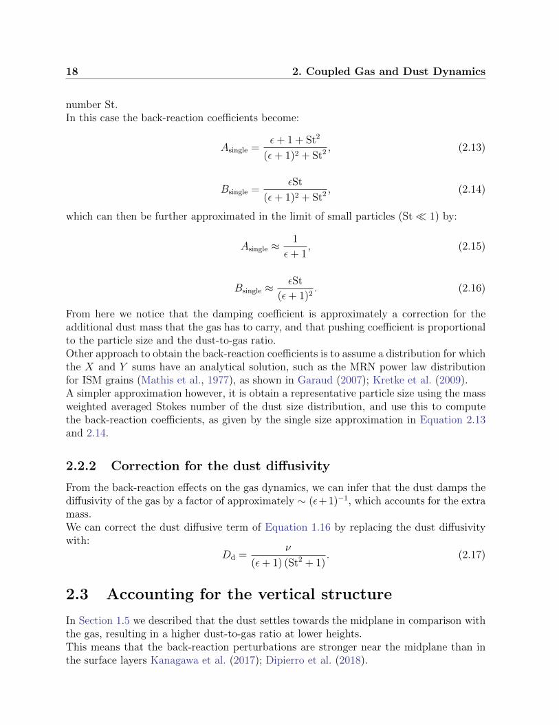
number St.In this case the back-reaction coefficients become:
Asingle =ε+ 1 + St2
(ε+ 1)2 + St2 , (2.13)
Bsingle =εSt
(ε+ 1)2 + St2 , (2.14)
which can then be further approximated in the limit of small particles (St 1) by:
Asingle ≈1
ε+ 1, (2.15)
Bsingle ≈εSt
(ε+ 1)2. (2.16)
From here we notice that the damping coefficient is approximately a correction for theadditional dust mass that the gas has to carry, and that pushing coefficient is proportionalto the particle size and the dust-to-gas ratio.Other approach to obtain the back-reaction coefficients is to assume a distribution for whichthe X and Y sums have an analytical solution, such as the MRN power law distributionfor ISM grains (Mathis et al., 1977), as shown in Garaud (2007); Kretke et al. (2009).A simpler approximation however, it is obtain a representative particle size using the massweighted averaged Stokes number of the dust size distribution, and use this to computethe back-reaction coefficients, as given by the single size approximation in Equation 2.13and 2.14.
2.2.2 Correction for the dust diffusivity
From the back-reaction effects on the gas dynamics, we can infer that the dust damps thediffusivity of the gas by a factor of approximately ∼ (ε+1)−1, which accounts for the extramass.We can correct the dust diffusive term of Equation 1.16 by replacing the dust diffusivitywith:
Dd =ν
(ε+ 1) (St2 + 1). (2.17)
2.3 Accounting for the vertical structure
In Section 1.5 we described that the dust settles towards the midplane in comparison withthe gas, resulting in a higher dust-to-gas ratio at lower heights.This means that the back-reaction perturbations are stronger near the midplane than inthe surface layers Kanagawa et al. (2017); Dipierro et al. (2018).

2.3 Accounting for the vertical structure 19
To account for the gas and dust vertical distribution, we must derive the radial velocity ofboth components from the net mass flux:
Σgvg,r =
∫ +∞
−∞ρg(z) vg,r(z) dz, (2.18)
Σd(m)vd,r(m) =
∫ +∞
−∞ρd(z,m) vd,r(z,m) dz. (2.19)
The volume densities of the gas and dust are defined by the gaussian profiles given inEquation 1.31 and 1.32. Notice that the argument of the integral in Equation 2.19 isweighted more heavily around the midplane for the larger particles than for smaller ones.Also, notice that small particles and the gas component present a similar vertical weight,since they have similar vertical structures.We model the gas velocity at every height:
vg,r(z) = A(z)vν + 2B(z)vP , (2.20)
where the back-reaction coefficients are now a function of the dust distribution at everyheight, with the local dust-to-gas ratio defined as εm(z) = ρd(m, z)/ρg(z).Using this expression we can rewrite Equation 2.18 as:
vg,r =1
Σg
∫ +∞
−∞ρg(z) (A(z) vν + 2B(z) vP ) dz = A vν + 2B vP , (2.21)
following (Garate et al., 2020). Now the information about the vertical distribution of gasand dust is included in the coefficients A and B, which are the mass weighted and verticallyaveraged back-reaction coefficients.This process can be repeated for the dust mass flux in order to obtain the dust velocitywhile accounting for the vertical structure.A more rigorous approach would be to also include the vertical structure of the viscous andpressure velocity as described in Kanagawa et al. (2017); Dipierro et al. (2018), howeverin our work we showed that the net flux does not change by considering this step (Garateet al., 2020).For reference, the viscous and pressure velocities can be modeled as:
vν(z) =ν
2r
(6p+ q − 3 + (5q − 9)
(z
hg
)2), (2.22)
vP (z) = vK
(hg
r
)2(p+
q + 3
2+q − 3
2
(z
hg
)2), (2.23)
following the Takeuchi & Lin (2002); Dipierro et al. (2018) model, with p and q the expo-nents of the gas surface density and temperature profiles respectively.

20 2. Coupled Gas and Dust Dynamics
2.4 Relevance of dust back-reaction
2.4.1 An analytical back-reaction condition
We now have the ingredients to assess how important is the back-reaction for the collectivedisk evolution.As in Dipierro et al. (2018); Garate et al. (2020), we notice that the viscous and pressurevelocity can be rewritten as:
vν = −3ανc2s
vKγν , (2.24)
vP = −1
2
c2s
vKγP , (2.25)
with γν = dln(ν Σg
√r)/dln r and γP = dlnP/dln r the power law exponents, which are on
the order of the unity in a smooth disk.To first order, the back-reaction is locally important for the gas dynamics if the pushingterm is comparable to the viscous term in the radial velocity (|2BvP | & |Avν |, Equa-tion 2.3). Using the single size approximation for the back-reaction coefficients, and therewritten expressions for the viscous and pressure velocities (Equation 2.15, 2.16, 2.24, and2.25) we rewrite this condition as:
St ε
α& 1. (2.26)
As would be expected, the most important parameters to determine the importance of thedust back-reaction are the Stokes number, the dust-to-gas ratio, and the turbulent viscosity.
2.4.2 Parameter space tests
To study the effect of the dust back-reaction on the disk velocity profiles, we construct asimple disk model in steady state with:
Σg(r) = 1000 g cm−2( r
1 AU
)−1
, (2.27)
T (r) = 300 K( r
1 AU
)−1/2
. (2.28)
We assume a mean molecular weight of µ = 2.3 for the gas. For the dust growth weassume that the particle size corresponds to the minimum between the fragmentation anddrift limits (Equation 1.28, 1.30), therefore we have a single particle size at each radius.Now we show the velocity profile for different dust-to-gas ratios, turbulence, and fragmen-tation velocity values. A detailed comparison between the gas velocity with back-reactionand the viscous velocity for static disk model can also be found in Dipierro et al. (2018).For now we calculate only a static solution with our toy model. In Chapter 3 we show the

2.4 Relevance of dust back-reaction 21
effects of dust back-reaction on disk evolution, including gas and dust advection, multipledust species and coagulation.
Fiducial Model
Parameter Valueε 0.01α 10−3
vfrag 1000 cm s−1
Table 2.1: Fiducial parameters for the analytical model.
100 101 102
r (AU)10 2
10 1
100
St
StStfrag
Stdrift
100 101 102
r (AU)
2
0
2
4
6v
(AU/
yr)
×10 5
Av2BvP
vg
Figure 2.1: Left : Stokes number profile for the fiducial analytical model (black). The frag-mentation and drift limits are marked with red and blue dotted lines, respectively. Right :Gas velocity profile for the fiducial model considering the back-reaction effect (black).The damped viscous component, and the pushing component are marked in red and blue,respectively.
For our fiducial model we use the parameters of Table 2.1. Figure 2.1 shows the Stokesnumber profile for our analytical disk model, in which the particle growth at inner regions(inside 100 AU) is limited by fragmentation, while at the outer regions is limited by drift.The gas velocity profile shows that, as the Stokes number increases, the back-reaction pushbecomes dominant for larger radii. Due to the back-reaction effect, the gas accretion isreversed beyond 3 AU, where the term 2BvP > Avν . These results indicate that even ina smooth disk (which under viscous evolution would flow inward), the back-reaction pushcan cause it to flow outwards if the particle sizes are large enough. From the velocity profilewe can expect the gas accretion onto the star to decrease, as the dust flow pushes the gasoutwards.We must notice however, that the back-reaction effects will stop as soon as the dust reservoir
22 2. Coupled Gas and Dust Dynamics
is depleted. In other words, the back-reaction perturbation are more likely to be effectiveduring early stages of disk evolution, while the dust content is high. After the dust driftstowards the star, the gas should retake the standard viscous evolution (Garate et al., 2020),if we do not consider the influence of dust traps. In Section 3.2 we will also show that thetime evolution and coagulation play a major role in reducing the effect of the back-reaction.
The effect of the dust-to-gas ratio
100 101 102
r (AU)
0.0
0.5
1.0
1.5
v g (A
U/yr
)
×10 4
= 0.01 = 0.03 = 0.05
100 101 102
r (AU)6
5
4
3
2
1
0
v d (A
U/yr
)
×10 3
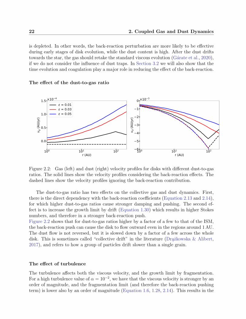
Figure 2.2: Gas (left) and dust (right) velocity profiles for disks with different dust-to-gasratios. The solid lines show the velocity profiles considering the back-reaction effects. Thedashed lines show the velocity profiles ignoring the back-reaction contribution.
The dust-to-gas ratio has two effects on the collective gas and dust dynamics. First,there is the direct dependency with the back-reaction coefficients (Equation 2.13 and 2.14),for which higher dust-to-gas ratios cause stronger damping and pushing. The second ef-fect is to increase the growth limit by drift (Equation 1.30) which results in higher Stokesnumbers, and therefore in a stronger back-reaction push.Figure 2.2 shows that for dust-to-gas ratios higher by a factor of a few to that of the ISM,the back-reaction push can cause the disk to flow outward even in the regions around 1 AU.The dust flow is not reversed, but it is slowed down by a factor of a few across the wholedisk. This is sometimes called “collective drift” in the literature (Drazkowska & Alibert,2017), and refers to how a group of particles drift slower than a single grain.
The effect of turbulence
The turbulence affects both the viscous velocity, and the growth limit by fragmentation.For a high turbulence value of α = 10−2, we have that the viscous velocity is stronger by anorder of magnitude, and the fragmentation limit (and therefore the back-reaction pushingterm) is lower also by an order of magnitude (Equation 1.6, 1.28, 2.14). This results in the
2.4 Relevance of dust back-reaction 23
100 101 102
r (AU)
1.5
1.0
0.5
0.0
0.5
1.0
1.5
v g (A
U/yr
)
×10 4
= 10 4
= 10 3
= 10 2
100 101 102
r (AU)
1.2
1.0
0.8
0.6
0.4
0.2
0.0
v d (A
U/yr
)
×10 2
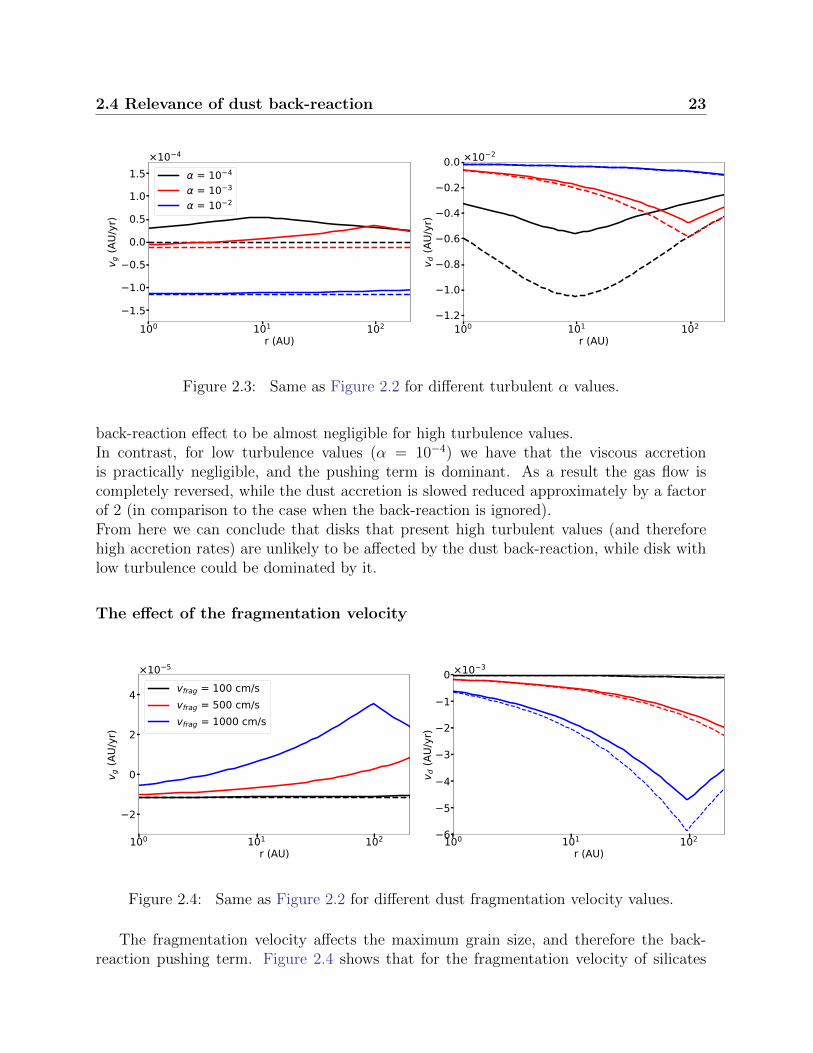
Figure 2.3: Same as Figure 2.2 for different turbulent α values.
back-reaction effect to be almost negligible for high turbulence values.In contrast, for low turbulence values (α = 10−4) we have that the viscous accretionis practically negligible, and the pushing term is dominant. As a result the gas flow iscompletely reversed, while the dust accretion is slowed reduced approximately by a factorof 2 (in comparison to the case when the back-reaction is ignored).From here we can conclude that disks that present high turbulent values (and thereforehigh accretion rates) are unlikely to be affected by the dust back-reaction, while disk withlow turbulence could be dominated by it.
The effect of the fragmentation velocity
100 101 102
r (AU)
2
0
2
4
v g (A
U/yr
)
×10 5
vfrag = 100 cm/svfrag = 500 cm/svfrag = 1000 cm/s
100 101 102
r (AU)6
5
4
3
2
1
0
v d (A
U/yr
)
×10 3
Figure 2.4: Same as Figure 2.2 for different dust fragmentation velocity values.
The fragmentation velocity affects the maximum grain size, and therefore the back-reaction pushing term. Figure 2.4 shows that for the fragmentation velocity of silicates
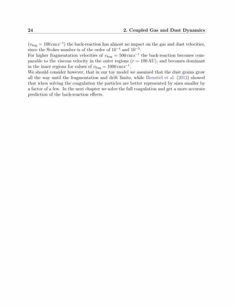
24 2. Coupled Gas and Dust Dynamics
(vfrag = 100 cm s−1) the back-reaction has almost no impact on the gas and dust velocities,since the Stokes number is of the order of 10−4 and 10−3.For higher fragmentation velocities of vfrag = 500 cm s−1 the back-reaction becomes com-parable to the viscous velocity in the outer regions (r ∼ 100 AU), and becomes dominantin the inner regions for values of vfrag = 1000 cm s−1.We should consider however, that in our toy model we assumed that the dust grains growall the way until the fragmentation and drift limits, while Birnstiel et al. (2012) showedthat when solving the coagulation the particles are better represented by sizes smaller bya factor of a few. In the next chapter we solve the full coagulation and get a more accurateprediction of the back-reaction effects.

Chapter 3
Effects of Dust Back-reaction in DiskEvolution
In this chapter we present different effects of the dust back-reaction on the evolution ofa protoplanetary disk, using numerical simulations to evolve gas and dust. We study theevolution of the following disks:
• A smooth self-similar disk (see Equation 1.11).
• A disk with a radial change in the fragmentation velocity, which causes a dust trafficjam (see Section 1.3, and Equation 1.28).
• A disk with a local pressure maximum, where dust accumulates (see Section 1.3).
This chapter is intended to serve as a general overview of the dust back-reaction effects, andas motivation for more complex models where the back-reaction might play an importantrole (see Garate et al., 2019, 2020, and Chapter 4, 5, and 6).
3.1 General setup in DustPy
We use the code DustPy (Stammler & Birnstiel, in prep.), which solves the gas and dusttransport in the radial direction following Equation 1.1 and 1.16, along with the Smolu-chowski coagulation equation for multiple dust species, as in Birnstiel et al. (2010).We include the dust back-reaction by modifying the gas and dust velocities using the back-reaction coefficients, as described in Section 2.1, 2.2 and 2.3.We use the parameters described in Table 3.1 for our numerical setup.Notice that here we distinguish between the turbulent viscosity αν , which affects the gasglobal viscous evolution, and the dust turbulence αt, which affects the small scale dustdynamics, such as fragmentation, diffusion, and settling.We use an initial dust-to-gas ratio of ε0 = 0.03 as fiducial value, and but also comparethe time evolution of the accretion rate to disks with other initial dust-to-gas ratios. Wepick a higher dust-to-gas ratio than the canonical ε0 = 0.01 of the ISM, as otherwise the

26 3. Effects of Dust Back-reaction in Disk Evolution
back-reaction effects are unnoticeable without including several dust trapping mechanismat the same time.The simulation grid is set according to Table 3.2.
Parameter Value DescriptionM∗ 1M Stellar massΣ0 1000 g cm−2 Surface density at r0
T0 300 K Temperature at r0
r0 1 AU Normalization radiusαν 10−3 turbulent viscosityαt 10−3 Dust turbulencevfrag 1000 cm s−1 Fragmentation velocityµ 2.3 Gas mean molecular weighta0 1 µm Dust initial sizeρs 1.6 g cm−3 Dust material densityε0 0.03 Initial dust-to-gas ratio
Table 3.1: Fiducial parameters for the numerical model.
Parameter Value Descriptionnr 250 Number of radial grid cellsnm 120 Number of mass grid cellsrin 5 AU Radial inner boundaryrout 300 AU Radial outer boundarymmin 10−12 g Dust mass lower limitmmax 105 g Dust mass upper limit
Table 3.2: Grid parameters for the numerical model.
3.2 Slowing viscous evolution
In this section we study the effects of dust back-reaction on the evolution of a disk followingthe Lynden-Bell & Pringle (1974) self-similar profile (Equation 1.11), using a cut-off radiusof 100 AU, and an initial dust-to-gas ratio of ε0 = 0.03.From Figure 3.1 we see that the back-reaction has little effect on the global disk evolutionover the first 0.15 Myrs. The only appreciable difference from the surface density profilesis that the dust-to-gas ratio is slightly higher in the inner regions when the back-reactionis considered, but the increment is basically negligible.From Figure 3.2 we see that the particles have a Stokes number of St ∼ 10−2. Since thedust-to-gas ratio is also of the order of ε ∼ 10−2, we have that the disk evolution shouldstill be mostly viscous dominated, since α & Stε (see Equation 2.26).

3.2 Slowing viscous evolution 27
101 102
r (AU)10 2
10 1
100
101
102
103
(g/c
m2 )
GasDust
101 102
r (AU)10 3
10 2
10 1BR - OnBR - OffInitial Condition
Figure 3.1: Left: Surface density of gas (red) and dust (blue) for a disk with a self-similarprofile, at 0.15 Myrs, considering the back-reaction effects (solid lines) and ignoring them(dashed lines). The difference between both is only a factor of a few percents. Right:Dust-to-gas ratio profiles. The initial condition is plotted in dotted lines for comparison.
The effect of the back-reaction on the disk dynamics is more evident by looking at thestellocentric accretion rate, and the gas radial velocity profile (see Figure 3.3). During thefirst 0.1 Myrs of the disk evolution (for the fiducial simulation with initial dust-to-gas ratioε0 = 0.03), the dust reaches its maximum size by sticking, and is able to reverse the gasaccretion during this phase. Without the dust back-reaction, the gas accretion rate shouldbe approximately Mg ≈ 5.0× 10⁻⁸ M/yr, instead, when the back-reaction is consideredthe flux is reversed to Mg ≈ −1.0× 10⁻⁹ M/yr.After a small fraction of the dust drifts inward following the pressure gradient the back-reaction effects decrease and the regular viscous accretion is resumed. For our disk modelthe back-reaction effects become negligible after 0.4 Myrs. From the velocity profiles wenotice that in the inner regions the back-reaction push opposes the viscous accretion (whichpoints inward), while in the outer regions the back-reaction push enhances the outwardviscous spreading. We find that at r ≈ 100 AU the back-reaction push is comparable tothe viscous spreading velocity, however we find unlikely that this contribution will affectthe overall disk size, as the viscous speed grows faster with radii than the back-reactionpush, and also because the latter will decrease within a drift timescale.Our results agree with the reduced the net mass accretion described in Kanagawa et al.(2017), though their results show a stronger back-reaction effect, since the fragmentationbarrier was not considered. We do not find the self-induced dust traps in the outer diskdescribed by Gonzalez et al. (2017).From this simulation we learn that the back-reaction by itself cannot perturb the globaldisk evolution, as the dust is quickly depleted by radial drift, and other mechanisms tocollect dust should be present in order to affect the gas and dust distributions.We find that the net effect of the back-reaction is less efficient when considering multiple

28 3. Effects of Dust Back-reaction in Disk Evolution
101 102
r (AU)10 2
10 1
2 × 10 2
3 × 10 24 × 10 2
6 × 10 2
St
101 102
r (AU)10 4
10 3
10 2
10 1
100
101
Size
(cm
)
87654321
01
dust
[g/c
m2 ]
Figure 3.2: Left: Mass weighted stokes number profile for a disk with a self-similar profile.Right: Dust surface density distribution. Both plots are taken at 0.15 Myr, when dust isstill abundant in the disk, for the simulation when the back-reaction is considered.
species and solving the coagulation equation, than for the toy model presented in Sec-tion 2.4, both due to the difference between the maximum particle size calculated with thesimple growth limits (see Equation 1.30 and 1.28) and the real representative size showedin Figure 3.2, and also due to the time evolution of the dust density distribution.However, we can infer that accretion events might be heavily influenced by the back-reaction, as this can lead to a reduced, or even reversed gas flow.This experiment served as motivation to study the back-reaction effects on the accretionof gas and dust of RW Aur (Gunther et al., 2018), where the high dust content might slowdown the gas accretion rate in the event of a dead zone reactivation (see Chapter 4 andGarate et al., 2019).
3.3 Dust accumulation at traffic jams
In this section we study the back-reaction effects in the case of a disk with a traffic jam.We set up our disk as described in Section 3.1. For the initial conditions we assume thatthe surface density follows a power law profile, and is in viscous steady state as describedin Section 1.1.1 and Equation 1.9.To create the traffic jam we consider a disk that presents a change in the fragmentationvelocity of the dust particles at a certain radius, such that:
vfrag =
1000 cm s−1 r ≥ 20 AU
100 cm s−1 r < 20 AU(3.1)
As described in Section 1.3 and in Birnstiel et al. (2010), a change in the fragmentationvelocity (as in Equation 3.1) is expected to increase the concentration of small dust grains

3.3 Dust accumulation at traffic jams 29
0.0 0.1 0.2 0.3 0.4 0.5t (Myr)
0.50
0.25
0.00
0.25
0.50
0.75
1.00
Mg(M
/yr)
×10 8
= 0= 0.01= 0.03
101 102
r (AU)2
1
0
1
2
3
v g (A
U/yr
)
×10 5
Av2BvP
vGas
Figure 3.3: Left: Accretion rate evolution (measured at 10 AU for different initial dust-to-gas ratios, for a disk with a self-similar profile. Right: Gas velocity profile (black) at0.15 Myrs, considering the back-reaction effects. The red and blue lines show respectivelythe damped accretion, and the pushing components.
in the inner regions, since the particles in the outer disk grow to larger sizes and drift fasterthan the particles in the inner disk.Figure 3.4 shows that at the fragmentation velocity transition the dust effectively accumu-lates towards the inner regions. After 0.36 Myr, the inner boundary (rin = 5 AU) presentsa dust-to-gas ratio between ε = 0.1 and ε = 0.2. At the transition (r = 20 AU) the dust-to-gas ratio reaches values of ε = 0.45 when the back-reaction is ignored, and ε = 0.75when the back-reaction is considered. After this point the outer disk has exhausted thedust supply, and the back-reaction effects will slowly decay with time(see more on Garateet al., 2020).The gas surface density in the inner regions is also reduced to a ∼ 75% of its initial value.This occurs of the radial variation of the back-reaction pushing term, due to the radialdependency of the particle size. From Figure 3.5 we see that the particles in the inner re-gions grow to smaller sizes (St ∼ 10−4, meaning that the back-reaction push is weak), whilein the outer disk the particles grow to larger sizes (St ∼ 10−2), where the back-reactionpush can slow down the gas flow. This causes the inner disk to get slowly depleted as thedust particles accumulate. The effect is smoothed down once the dust has moved from theouter regions to the inner regions, and the back-reaction push should vanish once the dustsupply is exhausted.In terms of the accretion rate we see how the back-reaction reduces the accretion flow intothe star (Figure 3.6). Without the dust back-reaction the disk should remain in steadystate, however due to the decrease in the gas density, and the damping due to the accu-mulation of dust in the inner regions, the accretion rate is reduced to a ∼ 66% of its initialvalue, for an initial dust-to-gas ratio of ε0 = 0.03, and to a ∼ 33% of its initial value foran initial dust-to-gas ratio of ε0 = 0.05.

30 3. Effects of Dust Back-reaction in Disk Evolution
101 102
r (AU)10 2
10 1
100
101
102
103
(g/c
m2 )
GasDust
101 102
r (AU)10 2
10 1
100
BR - OnBR - OffInitial Condition
Figure 3.4: Same as Figure 3.1, for the simulation with a traffic jam, at 0.36 Myr
Because the traffic jam and the associated back-reaction effects depend on the change inthe fragmentation velocity, we expect a similar outcome at the disk icelines (Vericel &Gonzalez, 2020), where the composition of the dust grains change due to the sublimationand recondensation of volatiles.Drazkowska & Alibert (2017) and Schoonenberg & Ormel (2017) showed that due to watervapor diffusion, the dust-to-gas ratio can also be further enhanced at the outer edge of thewater snowline, where particles are large. The dust back-reaction could further increasethis effect and provide ideal conditions for the formation of planetesimals. This idea wasfurther explored in Chapter 5 and Garate et al. (2020) , where we characterized the back-reaction effects at the water snowline.
3.4 Spreading of a dust ring
In this section we study the effect of the dust back-reaction in a disk with a dust trap. Asmentioned in Section 1.3, a dust trap can be any region with a local pressure maximum,where the drift speed of large particles becomes zero (Equation 1.23, assuming that thegas speed is low enough to allow for the particles to accumulate).To create a pressure maximum in the disk, we consider that the turbulent viscosity αν isnot uniform, and that the disk is in viscous steady state following Equation 1.9, such that:
Σg = Σ0
(r
r0
)−1αν,0αν(r)
, (3.2)
where αν,0 = 10−3, and αν(r) corresponds to a variable turbulent viscosity profile. For thetemperature profile we assume a simple power law profile with exponent q = 0.5.We want to study the cases of a dust ring formed by the presence of a gap and a bump in

3.4 Spreading of a dust ring 31
101 102
r (AU)10 4
10 3
10 2
10 1
St
101 102
r (AU)10 4
10 3
10 2
10 1
100
101
Size
(cm
)
87654321
01
dust
[g/c
m2 ]
Figure 3.5: Same as Figure 3.2, for the simulation with a traffic jam, at 0.36 Myr.
the gas surface density, since both cases form a pressure maximum in the disk. To form agap in the gas surface density we use the following αν profile:
αν,gap(r) = αν,0 ×
(1 + Aν exp
(−1
2
(r − rνwν
)2))
, (3.3)
where rν , Aν , and wν are respectively the location, the amplitude, and the standard devi-ation of the gaussian factor.Similarly, to create a bump in the gas surface density, we use the following αν profile.
αν,bump(r) = αν,0 ×
(1 + (1− Aν) exp
(−1
2
(r − rνwν
)2))
. (3.4)
For both the gap and the bump we set the location to rν = 20 AU, the amplitude toAν = 0.5, and the width to wν = 1.5 AU.Figure 3.7 shows the surface densities, dust-to-gas ratio, and gas velocity profiles for bothsetups, and Figure 3.9 shows the dust size distribution for the case when the back-reactionis considered.For the “local gap” simulation, the dust ring is formed at the outer edge of the gap (atr = 22 AU, where the pressure maximum is located), while for the “local bump” simulationthe dust ring is at rν = 20 AU, right at the center of the bump.Because the pressure maximum location and the steepness of the pressure gradient differsbetween the two scenarios, we can the properties of the dust trap do be quantitativelydifferent, as well as the back-reaction effects.The most evident effect of the back-reaction is that the dust ring is spread over a widerradii, and the maximum dust-to-gas ratio is lower. For the “local gap” simulation themaximum dust-to-gas ratio decreases from ε = 0.35 to ε = 0.20 when the back-reaction
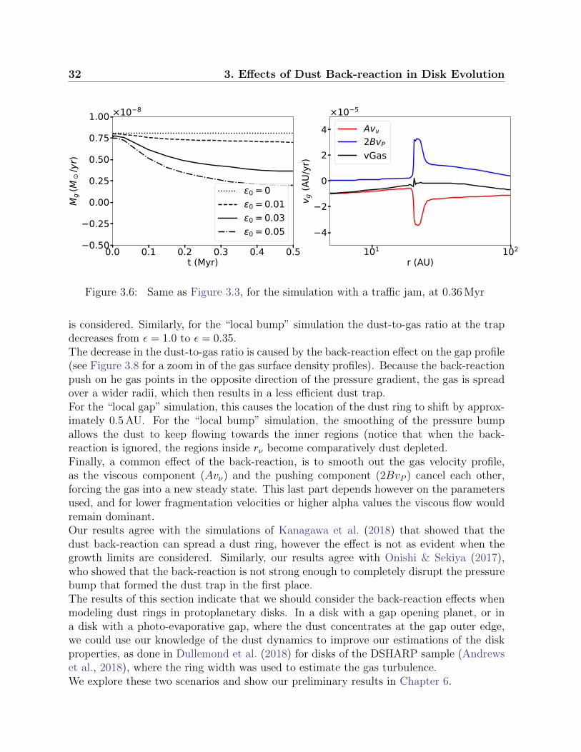
32 3. Effects of Dust Back-reaction in Disk Evolution
0.0 0.1 0.2 0.3 0.4 0.5t (Myr)
0.50
0.25
0.00
0.25
0.50
0.75
1.00
Mg(M
/yr)
×10 8
0 = 00 = 0.010 = 0.030 = 0.05
101 102
r (AU)
4
2
0
2
4
v g (A
U/yr
)
×10 5
Av2BvP
vGas
Figure 3.6: Same as Figure 3.3, for the simulation with a traffic jam, at 0.36 Myr
is considered. Similarly, for the “local bump” simulation the dust-to-gas ratio at the trapdecreases from ε = 1.0 to ε = 0.35.The decrease in the dust-to-gas ratio is caused by the back-reaction effect on the gap profile(see Figure 3.8 for a zoom in of the gas surface density profiles). Because the back-reactionpush on he gas points in the opposite direction of the pressure gradient, the gas is spreadover a wider radii, which then results in a less efficient dust trap.For the “local gap” simulation, this causes the location of the dust ring to shift by approx-imately 0.5 AU. For the “local bump” simulation, the smoothing of the pressure bumpallows the dust to keep flowing towards the inner regions (notice that when the back-reaction is ignored, the regions inside rν become comparatively dust depleted.Finally, a common effect of the back-reaction, is to smooth out the gas velocity profile,as the viscous component (Avν) and the pushing component (2BvP ) cancel each other,forcing the gas into a new steady state. This last part depends however on the parametersused, and for lower fragmentation velocities or higher alpha values the viscous flow wouldremain dominant.Our results agree with the simulations of Kanagawa et al. (2018) that showed that thedust back-reaction can spread a dust ring, however the effect is not as evident when thegrowth limits are considered. Similarly, our results agree with Onishi & Sekiya (2017),who showed that the back-reaction is not strong enough to completely disrupt the pressurebump that formed the dust trap in the first place.The results of this section indicate that we should consider the back-reaction effects whenmodeling dust rings in protoplanetary disks. In a disk with a gap opening planet, or ina disk with a photo-evaporative gap, where the dust concentrates at the gap outer edge,we could use our knowledge of the dust dynamics to improve our estimations of the diskproperties, as done in Dullemond et al. (2018) for disks of the DSHARP sample (Andrewset al., 2018), where the ring width was used to estimate the gas turbulence.We explore these two scenarios and show our preliminary results in Chapter 6.

3.4 Spreading of a dust ring 33
101 102
r (AU)10 1
100
101
102
103
(g/c
m2 )
Local GapGasDust
101 102
r (AU)10 1
100
101
102
103
(g/c
m2 )
Local Bump
101 102
r (AU)
10 2
10 1
100BR - OnBR - OffInitial Condition
101 102
r (AU)
10 2
10 1
100
101 102
r (AU)
5.0
2.5
0.0
2.5
5.0
v g (A
U/yr
)
×10 5
Av2BvP
vg
101 102
r (AU)
5.0
2.5
0.0
2.5
5.0
v g (A
U/yr
)
×10 5
Figure 3.7: Surface density profiles (top panel), dust-to-gas ratio profiles (middle panel),and gas velocity profiles along with the back-reaction components (bottom panel), for thesimulation with a dust ring formed by a density gap (left column), and by a density bump(right column). The profiles are taken at 0.15 Myr.

34 3. Effects of Dust Back-reaction in Disk Evolution
2 × 101 3 × 101
r (AU)
102
3 × 101
4 × 101
6 × 101
(g/c
m2 )
Local GapGas
2 × 101 3 × 101
r (AU)
102
3 × 101
4 × 101
6 × 101
(g/c
m2 )
Local Bump
Figure 3.8: Zoom in of the gas surface density profiles in Figure 3.7 top panel. The solidline shows the profiles considering the back-reaction effects, while the dashed lines ignoreit.

3.4 Spreading of a dust ring 35
101 102
r (AU)10 2
10 1
2 × 10 2
3 × 10 24 × 10 2
6 × 10 2
St
101 102
r (AU)10 4
10 3
10 2
10 1
100
101
Size
(cm
)87654321
01
dust
[g/c
m2 ]
101 102
r (AU)10 2
10 1
2 × 10 2
3 × 10 24 × 10 2
6 × 10 2
St
101 102
r (AU)10 4
10 3
10 2
10 1
100
101
Size
(cm
)
87654321
01
dust
[g/c
m2 ]
Figure 3.9: Mass weigthed stokes number profile (left column), and dust size distribution(right column) for the simulation with a dust ring formed by a density gap (top panel),and by a density bump (bottom panel). The profiles are taken at 0.15 Myr, for the casewhen the back-reaction is considered.

36 3. Effects of Dust Back-reaction in Disk Evolution

Chapter 4
An accretion event in RW Auriga?
The contents of this chapter where published in the Astrophysical Journal.Credit: The Dimming of RW Auriga: Is Dust Accretion Preceding an Outburst?,Garate et al., ApJ, 871, 53, 2019.c©AAS. Reproduced with permission.
4.1 Introduction
RW Aur A is a young star that in the last decade presented unusual variations in its lumi-nosity. The star has about a solar mass, it is part of a binary system, and is surroundedby a protoplanetary disk showing signatures of tidal interaction (Cabrit et al., 2006; Ro-driguez et al., 2018). The star had an almost constant luminosity for around a century,interrupted only by a few short and isolated dimmings (see Berdnikov et al. (2017) for ahistorical summary) until 2010, when its brightness suddenly dropped by 2 mag in the Vband for 6 months (Rodriguez et al., 2013). Since 2010, a total of five dimming events havebeen recorded (see Rodriguez et al., 2013, 2016; Petrov et al., 2015; Lamzin et al., 2017;Berdnikov et al., 2017, among others). The dimmings can last from a few months to twoyears, and reduce the brightness of the star up to 3 mag in the visual. Moreover, there isno obvious periodicity in their occurrence, and their origin is not yet clear (a summary ofthe events can be found in Rodriguez et al., 2018).
4.1.1 Observations of RW Aur Dimmings
Some observations in the recent years have shed light on the nature of RW Aur A dim-mings:During the event in 2014-2015 (Petrov et al., 2015), observations by Shenavrin et al. (2015)show a increase in IR luminosity at bands L and M. The authors infer that hot dust fromthe inner regions is emitting the infrared excess, while occluding the starlight and causingthe dimming in the other bands.Observations by Antipin et al. (2015); Schneider et al. (2015) found that the absorption

38 4. An accretion event in RW Auriga?
from optical to NIR wavelengths is gray, which could indicate the presence of large particlescausing the dimming (& 1µm), and measured a dust column density of 2× 10⁻⁴ g/cm2,although a similar absorption may be produced if an optically thick disk of gas and smallgrains partially covers the star (Schneider et al., 2018).Then, the study of RW Aur A spectra by Facchini et al. (2016) also found that the inneraccretion regions of the disk are being occluded, and therefore the dimmings should comefrom perturbations at small radii.Finally, during the dimming in 2016, X-Ray observations from Gunther et al. (2018) indi-cate super-Solar Fe abundances, along with a higher column density of gas in the line ofsight. The high NH/AV found by the authors is interpreted as gas rich concentrations inthe occluding material, or as a sign of dust growth. Also, gray absorption was found againduring this event.Given this information, several authors have discussed what mechanism would put thedust from the innermost regions of the protoplanetary disk, into the line of sight. Amongthe possible explanations are: a warped inner disk (Facchini et al., 2016; Bozhinova et al.,2016), stellar winds carrying the dust (Petrov et al., 2015; Shenavrin et al., 2015), plan-etesimal collision (Gunther et al., 2018), and a puffed up inner disk rim (Facchini et al.,2016; Gunther et al., 2018).Most of the proposed mechanisms rely on having enough dust close to the star to causethe dimmings. So the focus of this study is to propose a mechanism that can deliver largeamounts of dust to the inner regions of the protoplanetary disk, by raising the dust accre-tion rate through the release of a dust trap.An increased dust concentration can explain some aspects of the dimmings, such as thehigh metallicity (Gunther et al., 2018), the emission of hot dust (Shenavrin et al., 2015),and cause the dimmings provided that another mechanism transports it into the line ofsight.
4.1.2 A Fast Mechanism for Dust Accretion
A sudden rise in the dust accretion can occur in the early stages of stellar evolution, whenthe stars are still surrounded by their protoplanetary disk composed of gas and dust. Thedynamics of the gas component of the disk is governed by the viscous evolution, whichdrives the accretion into the star (Lynden-Bell & Pringle, 1974), and the pressure support,that produces the sub-keplerian motion. On the other hand, the dust particles are notaffected by pressure forces, but suffer the drag force from the gas. This interaction ex-tracts angular momentum from the particles and causes them to drift towards the pressuremaximum, with the drift rate depending on the coupling between the dust and gas mo-tion (Whipple, 1972; Weidenschilling, 1977; Nakagawa et al., 1986). This means that anybumps in the gas pressure act as concentration points for the dust. In these dust traps thegrains accumulate, grow to larger sizes, and reach high dust-to-gas ratios (Whipple, 1972;Pinilla et al., 2012).One of the proposed mechanisms to generate a pressure bump is through a dead zone(Gammie, 1996), a region with low turbulent viscosity (the main driver of accretion), due

4.2 Model Description 39
to a low ionization fraction which turns off the magneto-rotational instability (Balbus &Hawley, 1991), that allows the gas to accumulate until a steady state is reached.The presence of a dead zone would allow the dust to drift and accumulate at its innerborder (Kretke et al., 2009), which can be located at the inner regions of the protoplane-tary disk (r . 1 au). Assuming that these conditions are met, the reactivation of the deadzone turbulent viscosity through thermal, gravitational or magnetic instabilities (Martin &Lubow, 2011) would break the steady state and allow all the accumulated material (bothgas and dust), to be flushed towards the star. This mechanism has been invoked alreadyin the context of FU Ori objects to explain the variability in their accretion rate throughoutbursts (Audard et al., 2014).Since the dust is drifting faster than the gas, because of hydrodynamic drag and dustdiffusion, it will arrive at the inner boundary of the disk first, where it may generate theobserved hot dust signatures, Fe abundances, and the dimmings if it enters into the lineof sight through either a puffed up inner rim, or a stellar wind (among the explanationsmentioned above). Therefore, the accretion of large amounts of dust could be actuallyfollowed by an increase in the gas accretion rate.In this study we use 1D simulations of gas and dust, including dust coagulation and frag-mentation, to model the concentration of dust at the inner edge of a dead zone. Subsequentreactivation of the turbulent viscosity lets the accumulated material rapidly drift towardsthe star. We measure the timescale required for the dust drifting, how much dust can beconcentrated into the inner regions by this mechanism, and put it into the context of theobserved features during the dimmings along with the possible explanations listed.
4.2 Model Description
For our disk model we evolve the gas and dust according to the advection equations de-scribed in Chapter 1, assuming that the disk evolves through viscous evolution, and thatthe dust and gas interact through the drag force. In the simulations where we consider thedust back-reaction, we do so as described in Chapter 2.Here we present the description of our dead zone model, and its reactivation.
4.2.1 Dead Zone Model
Magneto-hydrodynamical models have predicted the presence of a region with low turbu-lence at the inner regions of protoplanetary disks, commonly called “Dead Zone”, causedwhen the ionization fraction is too low for the magneto-rotational instability (MRI) tooperate (Gammie, 1996).We parametrize the dead zone by using a variable α parameter over radius, while remainingagnostic to the underlying physics, similar to previous research (Kretke et al., 2009; Pinilla

40 4. An accretion event in RW Auriga?
r1 r2r
dead
active
Figure 4.1: The diagram shows the shape of the α radial profile for our dead zone model(in logarithmic scale). This consists on three regions, the active inner zone limited by asharp decay at r1, the dead zone with a smooth rise towards its outer edge around r2, andthe outer active zone extending until the outer boundary of the simulation.
et al., 2016). Our profile is defined as:
α(r) =
αactive −∆α · e5( r
r1−1)
r < r1
αdead + ∆α · 12e
10( rr2−1)
r1 < r < r2
αdead + ∆α · (1− 12e−10( r
r2−1)
) r2 < r,
(4.1)
where αdead and αactive are the characteristic values of the α parameter inside and outsidethe dead zone, r1 and r2 are its inner and outer edges, and ∆α = αactive−αdead. Althoughthe dead zone shape is rather arbitrary, it was chosen to have a smoother outer borderthan the one of (Kretke et al., 2009), but retaining a sharp inner edge where the dustaccumulates. Figure 4.1 shows a diagram of the α profile, illustrating the shape of thedifferent intervals and its main components to guide the reader with Equation 4.1.
In order to maintain the steady state from Equation 1.9 we define the initial surfacedensity and temperature profiles as follow:
Σg(r) = Σg,0
(r
r0
)−1αactive
α(r), (4.2)
T (r) = T0
(r
r0
)−1/2
, (4.3)
where Σ0 and T0 are the values of the density and temperature at r0 = 1 au.

4.3 Simulation Setup 41
4.2.2 Dead Zone Reactivation
While the dead zone is present the gas will remain in steady state and the dust willaccumulate at its inner boundary. Yet, different processes can reactivate the turbulencein the dead zone, allowing the accumulated material to flush towards the star. In theGravo-Magneto instability (Martin & Lubow, 2011) for example, the gas in the dead zonebecomes gravitationally unstable, raising the temperature to the point of triggering theMRI, and finally producing an accretion outburst.In our simulations we remain agnostic about the mechanism that causes the reactivation,and only set the reactivation time tr arbitrarily, such that:
α(r, t > tr) = αactive. (4.4)
4.3 Simulation Setup
In this section we describe the observational constrains relevant for RW Aur A, the freeparameters of our model, and the setup of our 1D simulations using the twopoppy (Birn-stiel et al., 2012) and DustPy1 (Stammler & Birnstiel, in prep.) codes.Our setup consists of three phases, the first phase simulates the dust accumulation at thedead zone, using a global disk simulation over long timescales (∼ 105 yr), but with a simpli-fied and fast computational model for the dust distribution using only two representativepopulations. As the first phase only tracks the evolution of the surface density, in a secondphase we recover the quasi-stationary particle size distribution at the inner disk (r ≤ 5 au)by simulating the dust growth and fragmentation of multiple dust species. Finally, thethird phase simulates evolution of gas and dust (including coagulation, fragmentation, andtransport) in the inner disk after the dead zone is reactivated, to study the accretion ofthe accumulated material towards the star over short timescales, and delivering the finalresults.This setup is useful to save computational time, as we are interested only in the inner diskafter the dead zone reactivation, but require the conditions given by the global simulation.
4.3.1 Observational Constrains
RW Aur A is a young star with a stellar mass of M∗ = 1.4 M (Ghez et al., 1997; Woitaset al., 2001). The circumstellar disk has an estimated mass around Mdisk ≈ 4× 10⁻³ M(Andrews & Williams, 2005), presents a high accretion rate of M ≈ 4× 10⁻⁸−2× 10⁻⁷ M/yr(Hartigan et al., 1995; Ingleby et al., 2013; Facchini et al., 2016), and extends from a dis-tance of ∼ 0.1 au (Akeson et al., 2005; Eisner et al., 2007) until 58 au (Rodriguez et al.,2018).For the temperature profile we use T0 = 250 K, which gives similar values to the Osterloh& Beckwith (1995) profile in the inner regions of the disk for our choice of slope.
1DustPy is a new Python code that solves the diffusion-advection of gas and dust, and the coagulation-fragmentation of dust, based on the Birnstiel et al. (2010) algorithm.

42 4. An accretion event in RW Auriga?
Using these parameters, Equation 1.4 and Equation 1.9, we can constraint the valuesfor the density and turbulence. From the disk accretion rate, mass and size we in-fer the value for the density Σ0 = 50 g/cm2 at r0 = 1 au, and the turbulent viscosityαactive = 0.1. These parameters yield values of Mg = 5× 10⁻⁸ M/yr for the accretionrate, and Mdisk = 2× 10⁻³ M for the disk mass (without considering the accumulationexcess in the dead zone). The turbulence parameter αactive used in our simulations is high,but necessary in order to account for the high accretion rates measured.
4.3.2 Phase 1: Dust Concentration at the Dead Zone
In the first phase of our simulations we model the accumulation of dust in a disk with adead zone, to obtain the dust-to-gas ratio radial profile.We use the TwoPopPy code to simulate a global protoplanetary disk with two representa-tive populations of the dust species (details of the model can be found in Birnstiel et al.,2012). We initialize our simulations using Equation 4.1, Equation 4.2 and Equation 4.3 forthe α parameter, surface gas density and temperature profiles, with the values provided bythe observational constrains. For the dust-to-gas ratio we assume an uniform initial valueof ε = 0.01.For this phase, the simulation domain goes from rin = 0.01 au to rout = 100 au, usingnr = 500 radial grid cells with logarithmic spacing. In the fiducial model, the inner andouter boundaries of the dead zone are r1 = 0.51 au, r2 = 10 au, with a depth of αdead = 10−4.The simulation is evolved with this setup until the reactivation time tr = 105yrs. Approxi-mately at this point the dust reaches its maximum accumulation at the inner boundary ofthe dead zone, which will yield the maximum dust accretion rate in the next phase. Sincethe gas is in steady state, we only evolve the dust in order to minimize possible numericalerrors. Inside the dead zone, the gas phase is (marginally) gravitationally stable, with aToomre parameter Q = csΩK/(πGΣg) & 1.5 (Toomre, 1964). A low Q value in this regiondoes not conflict with the model, since the gravitational instability is one of the mecha-nisms that can eventually reactivate the dead zone.The initial and final states of phase 1 are shown in Figure 4.2. During this phase the dustdrifts towards the dead zone inner edge reaching values of ε = 0.24, and concentrating110 M⊕ between 0.51 - 0.6 au. Due to diffusion, the dust concentration at the innermostpart of the disk also increases to values up to ε ≈ 0.16.
4.3.3 Phase 2: Dust Size Distribution at the Inner Disk
In the second phase we want to recover the dust size distribution for multiple species, basedon the dust-to-gas ratio and disk conditions obtained in the previous section.We take the outcome of the TwoPopPy simulation as the new initial conditions, and usethe DustPy code to solve the dust coagulation and fragmentation (following the studyof Birnstiel et al., 2010) at the inner disk, while “freezing” the simulation exactly at thereactivation time t = tr, while the dead zone is still present (i.e. still using Equation 4.1).The mass grid consists of nm = 141 logarithmic-spaced cells, between m = 10−15 − 105 g,

4.3 Simulation Setup 43
10 1 100 101
r (AU)
10 2
10 1
100
101
102
103
104
105
106
(g/c
m2)
Dust and Gas Densities
GasDust (t0 = 0 yrs)Dust (tr = 105 yrs)
Figure 4.2: Gas and dust surface density obtained from TwoPopPy, at the beginning andat the end of the dust concentration phase. The gas (red) remains in steady state duringthis phase. The dust is initialized with a dust-to gas ratio of ε = 0.01 (dashed blue line).The dust component is evolved for 105 yrs (solid blue line) in which the dust concentratesat the inner disk, reaching ε ≈ 0.24 at the inner boundary of the dead zone, and ε ≈ 0.16inside this region r < r1 = 0.51 au.
at every radius. Since in this phase we only care about the inner disk, we adjust oursimulation radial domain to be from rin = 0.05 au to rout = 5 au. The radial grid is definedas follow:
• 25 linear-spaced grid cells at r = 0.05− 0.09 au,
• 120 logarithmic-spaced grid cells at r = 0.09− 1.0 au,
• 20 logarithmic-spaced grid cells at r = 1.0− 5.0 au.
The innermost region is necessary to avoid numerical problems with the inner boundaryconditions. For optimization purposes we also turn off coagulation for r < 0.09 au, since thegrowth and fragmentation timescales are so short in this region that the simulation becomescomputationally unfeasible. Moreover, according to Akeson et al. (2005); Eisner et al.(2007) the inner boundary of RW Aur A disk should be around r ∼ 0.1− 0.2 au. For thesereasons all our analysis will only focus on the region of interest between r = 0.1− 1.0 au.We interpolate the gas and dust surface densities from the TwoPopPy simulation intothe new grid, and use the coagulation model of DustPy to obtain the corresponding sizedistribution of the particles at t = tr for every radius. The dust distribution obtained atthis phase is shown in Figure 4.3, where the grains adjust to the fragmentation limit in thedead and active zones.

44 4. An accretion event in RW Auriga?
0.1 0.2 0.3 0.4 0.5 0.6 0.7r (AU)
10 4
10 3
10 2
10 1
100
101
Size
(cm
)
Time: tr + 0.0 yr
54321
01234
dust
[g/c
m2 ]
Figure 4.3: Dust distribution in the inner region of the protoplanetary disk immediatelybefore the dead zone reactivation (t = tr). In the dead zone, where the turbulence and thecollision speed of solids are lower, the dust particles can grow to larger sizes (amax ∼ 1 cm)before reaching the fragmentation limit. At the active zone, the particles are respectivelysmaller (amax ∼ 10µm). The inner edge of the dead zone (marked by the white line)presents a high concentration of large dust grains.
4.3.4 Phase 3: Dead Zone Reactivation
For the final phase we simulate the evolution of dust and gas in the inner disk, after thereactivation of the dead zone (t > tr).Once again we use the DustPy code, this time to solve the advection of gas and dust, alongwith the dust coagulation-fragmentation. We start this phase from the conditions givenat Section 4.3.3, using the same grid for mass and radius, but now with the reactivatedturbulence following Equation 4.4. We let the simulation evolve for 15 yrs, in which weexpect that the material accumulated at the inner boundary of the dead zone will drifttowards the star. The results of this phase on the accretion rate of gas and dust, as wellas the final dust distribution, will be shown in Section 4.4.2
4.3.5 Parameter Space
In Table 4.1 we summarize the parameters used for the disk setup of our fiducial simulation.As the properties of the dead zone are free parameters, chosen to be in a relevant rangefor the RW Aur dimming problem, we also require to explore (even briefly) the parameterspace for these properties, and see how they affect the final outcome of the simulations.We present five additional simulations, changing one parameter of the fiducial model at atime, this way we explore the effect of having: no initial dust accumulation at reactivation,
2The simulation data files and a plotting script are available in zenodo:doi.org/10.5281/zenodo.1495061.

4.4 Dead Zone Reactivation Results 45
Table 4.1: Fiducial simulation parameters.
Parameter ValueΣ0 50 g/cm2
T0 250 Kr0 1 auαactive 10−1
αdead 10−4
r1 0.51 aur2 10 autr 105 yrsBack-reaction Off
Table 4.2: Parameter variations.Simulation Parameter ChangedControl Simulation tr = 0 yrsShallow Dead zone αdead = 10−3
Closer Inner Edge r1 = 0.25 auCloser Outer Edge r2 = 4 auBack-reaction On
different dead zone properties, and the expected effects of back-reaction in the final result.The parameter changes are described in Table 4.2.
4.4 Dead Zone Reactivation Results
In this section we show the results obtained on the dust and gas dynamics after the “deadzone reactivation phase” (Section 4.3.4), including the final dust distribution, the dust-to-gas ratio at the inner boundary, and accretion rates of dust and gas. We also study theimpact of the dead zone parameters on the final outcome, to see if these results follow theexpected behavior.The gas and dust surface densities before and after the reactivation are shown in Figure 4.4.The initial surface density obtained from the first accumulation phase shows a dust-to-gasratio of ε = 0.24 at the dead zone inner edge, and ε = 0.16 in the inner disk (r . 0.5 au).After the reactivation (t > tr) the dust accumulated at the dead zone is transportedtowards the inner regions faster than the gas, reaching the inner boundary of the disk(rin ∼ 0.1− 0.2 au (Akeson et al., 2005; Eisner et al., 2007)) in only 15 years.Given that the surface density of dust at the dead zone edge was higher than the gassurface density at the inner regions, this leads to higher concentrations of dust than gasafter the reactivation (ε > 1). This should obviously make the dust dynamically important

46 4. An accretion event in RW Auriga?
0.1 0.2 0.3 0.4 0.5 0.6 0.7r (AU)
101
102
103
104
105
106
(g/c
m2)
DensityGasDust
0.1 0.2 0.3 0.4 0.5 0.6 0.7r (AU)
10 2
10 1
100
101
d/g
Dust-to-Gas RatioTime: tr + 15.0 yrTime: tr + 0 yr
Figure 4.4: The plots show the simulation state immediately before the dead zone reacti-vation at t = tr (dashed lines), and 15 yrs after it (solid lines). Top: Evolution of the gas(red) and dust (blue) surface densities. The initial state shows the gas steady state profileand the accumulation of dust at the inner boundary of the dead zone. After reactivationthe accumulation of dust flushes towards the star faster than the gas. Bottom: Dust-to-gasratio evolution. At the initial state the inner region presents an already high solid concen-tration thanks to mixing at the dead zone boundary. During the flushing the dust-to-gasratio reaches values of ε = 5 at some of the regions where the dust concentration arrivedbefore the gas.

4.4 Dead Zone Reactivation Results 47
0.1 0.2 0.3 0.4 0.5 0.6 0.7r (AU)
10 4
10 3
10 2
10 1
100
101
Size
(cm
)
Time: tr + 0.05 yr
54321
01234
dust
[g/c
m2 ]
0.1 0.2 0.3 0.4 0.5 0.6 0.7r (AU)
10 4
10 3
10 2
10 1
100
101
Size
(cm
)
Time: tr + 15.0 yr
54321
01234
dust
[g/c
m2 ]
Figure 4.5: Dust distribution in the inner region of the protoplanetary disk after0.05 and 15 yrs of the dead zone reactivation. Top: The dust that was accumulated atthe dead zone diffuses to the inner region within ∼ 10 collisional times, generating highdust-to-gas concentrations. The original edge of the dead zone is marked in white. Bot-tom: Afterwards, the dust drifts towards the inner disk regions (r ∼ 0.1 − 0.2 au) within∼ 15 yrs, while adjusting to the new fragmentation limit.
0 2 4 6 8 10 12 14Time (yr)
10 8
10 7
10 6
10 5
M (M
/yr)
Accretion rate at r: 0.15 AUGasDust
Figure 4.6: Accretion rate of gas (red) and dust (blue) at r = 0.15 au for 15 yrs afterthe dead zone reactivation. The initial gas accretion rate is Mg = 5× 10⁻⁸ M/yr, inagreement with the observations of RW Aur A, while the dust accretion rate is Md =7× 10⁻⁹ M/yr. Upon reactivation the dust accretion rate increases faster than the gas,eventually surpassing it after 10 yrs, and reaching a high value of Md = 6× 10⁻⁶ M/yr.

48 4. An accretion event in RW Auriga?
to the gas motion, however we shall see later in this section that as the particles are toosmall (St < 10−3), the only impact of dust back-reaction is to slow down the dust and gasevolution. Therefore no instabilities are generated and we can proceed with our analysis.Upon entering the active zone the particles fragment due to the high turbulence and adjustto their fragmentation limit (see Equation 1.28) in a few collisional timescales tcoll, whichcan be approximated by:
tcoll = (ndσ∆vturb)−1, (4.5)
where nd is the number density of dust particles, σ ≈ 4πa2 is the collisional cross section,and ∆vturb ≈
√3αStcs is the turbulent collision speed (Ormel & Cuzzi, 2007).
We find that during 10 collisional timescales (t ∼ 0.05 yrs) after the dead zone reactivationthe dust grains diffuse inward faster than the gas, gaining a head start that leads tohigh dust-to-gas ratio concentrations. We attribute this feature to the sudden rise in theturbulence α at the dead zone inner edge, that increases the dust diffusivity and spreadsthe particles towards the inner regions (see Equation 1.25 and Figure 4.5). After the dusthas adjusted to the new fragmentation limit, it drifts roughly with the viscous velocityof the gas vν towards the inner boundary of the disk. The particles reaching the innerboundary reach maximum sizes between amax = 10−100µm (see Figure 4.5).The accretion rate (measured at r = 0.15 au) of both dust and gas increases after thereactivation of the dead zone, as the accumulated material arrives at the inner boundaryof the disk (see Figure 4.6). Before the dead zone reactivation, the gas accretion rate isgiven by the steady state solution with Mg = 5× 10⁻⁸ M/yr, similar to the observationalvalue of (Facchini et al., 2016; Ingleby et al., 2013), and the dust accretion rate is Md =7× 10⁻⁹ M/yr, this value comes from the dust diffusing into the inner disk during theconcentration phase.After the dead zone reactivation the dust concentration moves inwards, and the accretionrate at the inner boundary of the disk becomes dominated by the dust, to the point ofsurpassing that of the gas. This high supply of solid material, with Md = 6× 10⁻⁶ M/yrcould cause hot dust and metallicity features of RW Aur A (Shenavrin et al., 2015; Guntheret al., 2018), and provide an ideal environment for the dimmings to occur (see Section4.5.1). At this point we also note that the accretion rate of gas has increased up toMg = 10−6 M/yr.In Section 4.5 we will discuss how the high accretion of solids could cause the dimmings inthe context of previous proposed mechanisms (dusty winds, puffed-up inner disk rim, etc),and if we can expect future accretion signatures from the gas. In the following subsections,we study the effect of the simulation parameters on the dust dynamics.
4.4.1 Simulation without Dust Concentration
In our model we remained agnostic to the reactivation process of the dead zone, and allowedthe dust to accumulate for long enough time to reach concentrations as high as ε = 0.24 atits inner edge. Depending on the mechanism that reactivates turbulence, the flushing ofsolid material towards the star may occur earlier with lower dust concentrations, reducing

4.4 Dead Zone Reactivation Results 49
0.1 0.2 0.3 0.4 0.5 0.6 0.7r (AU)
100
101
102
103
104
105
106
(g/c
m2)
Control - Density (Time: tr)Gas (Fiducial)Dust (Fiducial)Gas (Control)Dust (Control)
0.1 0.2 0.3 0.4 0.5 0.6 0.7r (AU)
100
101
102
103
104
105
106
(g/c
m2)
Density (Time: tr + 15.0 yr)
0.1 0.2 0.3 0.4 0.5 0.6 0.7r (AU)
10 2
10 1
100
101
d/g
Dust-to-Gas Ratio (Time: tr + 15.0 yr)FiducialControl
Figure 4.7: Comparison between the “fiducial” simulation (tr = 105 yrs, solid lines) andthe “control” simulation (tr = 0 yrs, dashed lines). Top: Gas and dust densities at thereactivation time (t = tr). In both cases the gas is in steady state, but in the controlsimulation the dust did not had the time to accumulate at the inner edge of the dead zone,in this case the reactivation occurs with a uniform dust-to-gas ratio ε = 0.01. Mid : Gasand dust densities after the dead zone reactivation (t = tr + 15 yrs). The dust that was atthe dead zone in steady state still arrives faster than the gas to the inner boundary of thedisk. Bottom: Dust-to-gas ratio after the reactivation. The maximum dust concentrationin the “control” simulation is now ε = 0.28.

50 4. An accretion event in RW Auriga?
the total accretion of solids. To model the limit case in which no dust concentration occurs,we repeat our setup with a control simulation, but now setting the reactivation time totr = 0 yrs.In Figure 4.7 we show the initial and final state of both simulations. Here the control sim-ulation has an uniform ε = 0.01 in the beginning, since no additional dust concentrationhas occurred. Notice that we still assume that the gas has reached the steady state densityprofile.After the reactivation the gas and dust excess at the dead zone drift towards the star. Asin the fiducial case, the dust that was located at the dead zone inner edge arrives at theinner boundary of the disk before the gas, also in a time of ∼ 15 yrs. The only differenceis that now the material being accreted has a dust-to-gas ratio of ε = 0.28, which is stillhigher than the initial ε = 0.01, although not as extreme as the ε = 5 found in the fiducialcase. Here the dust accretion rate at the inner boundary of the disk (r ≈ 0.15 au) canreach up to Md = 3× 10⁻⁷ M/yr.From here we learn that the dust arrival time at the inner boundary does not depend onthe amount of solids accumulated at the dead zone inner edge, and that upon reactivationthe accreted material will still carry a high concentration of solids.
4.4.2 Simulations for Different Dead Zone Properties
The dead zone shape is parametrized by its edges r1 and r2, and the turbulence parameterαdead following Equation 4.1, and altering these parameters also changes arrival time anddust-to-gas ratio of the accreted material.By shifting the inner edge of the dead zone to smaller radii (r1 = 0.51 au → 0.25 au) thedust concentration during the first phase will also be located closer to the inner boundaryof the disk (see Figure 4.8). Now it only takes the dust between 3−5 yrs to reach the innerboundary of the protoplanetary disk. Therefore the inner edge of the dead zone regulatesthe time required between the reactivation and the accretion of the dusty material.A dead zone with a closer outer boundary (r2 = 10 au→ 4 au) will be smaller and concen-trate less dust at its inner boundary (see Figure 4.9). This also reduces the total amountof solid material that it is accreted towards the star, although this is still a considerableamount with a dust-to-gas ratio of ε = 2.1.Finally, the most significant parameter is the turbulence αdead of the dead zone. Ourfiducial simulation considered an αdead = 10−4, which in contrast with the active zoneαactive = 10−1 leads to an accumulation of material in the dead zone with a factor of 1000relative to the steady state of a fully active disk, this of course favors the accretion ofmassive amounts of gas and solids upon reactivation. By taking a shallower dead zone(αdead = 10−4 → 10−3) there is less gas and dust accumulated, so upon reactivation theflushing of material is slower by a factor of a few (see Figure 4.10). We also find thatfor αdead = 10−3 there is no significant concentration at the dead zone inner edge, after105 yrs the dust-to-gas ratio rises only up to ε = 0.012. This happens because the higherturbulence lowers the fragmentation limit (see Equation 1.28), producing particles that
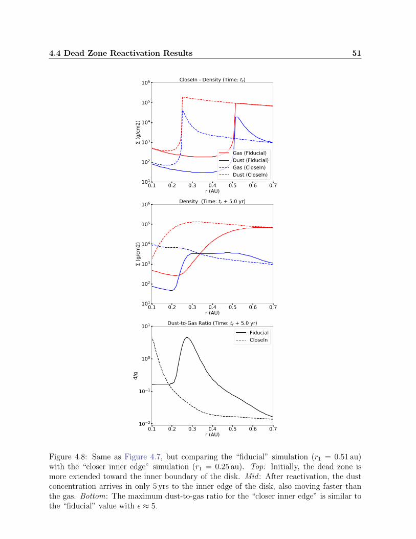
4.4 Dead Zone Reactivation Results 51
0.1 0.2 0.3 0.4 0.5 0.6 0.7r (AU)
101
102
103
104
105
106
(g/c
m2)
CloseIn - Density (Time: tr)
Gas (Fiducial)Dust (Fiducial)Gas (CloseIn)Dust (CloseIn)
0.1 0.2 0.3 0.4 0.5 0.6 0.7r (AU)
101
102
103
104
105
106
(g/c
m2)
Density (Time: tr + 5.0 yr)
0.1 0.2 0.3 0.4 0.5 0.6 0.7r (AU)
10 2
10 1
100
101
d/g
Dust-to-Gas Ratio (Time: tr + 5.0 yr)FiducialCloseIn
Figure 4.8: Same as Figure 4.7, but comparing the “fiducial” simulation (r1 = 0.51 au)with the “closer inner edge” simulation (r1 = 0.25 au). Top: Initially, the dead zone ismore extended toward the inner boundary of the disk. Mid : After reactivation, the dustconcentration arrives in only 5 yrs to the inner edge of the disk, also moving faster thanthe gas. Bottom: The maximum dust-to-gas ratio for the “closer inner edge” is similar tothe “fiducial” value with ε ≈ 5.

52 4. An accretion event in RW Auriga?
0.1 0.2 0.3 0.4 0.5 0.6 0.7r (AU)
101
102
103
104
105
106
(g/c
m2)
CloseOut - Density (Time: tr)Gas (Fiducial)Dust (Fiducial)Gas (CloseOut)Dust (CloseOut)
0.1 0.2 0.3 0.4 0.5 0.6 0.7r (AU)
101
102
103
104
105
106
(g/c
m2)
Density (Time: tr + 15.0 yr)
0.1 0.2 0.3 0.4 0.5 0.6 0.7r (AU)
10 2
10 1
100
101
d/g
Dust-to-Gas Ratio (Time: tr + 15.0 yr)FiducialCloseOut
Figure 4.9: Same as Figure 4.7, but comparing the “fiducial” simulation (r2 = 10 au) andthe “closer outer edge” simulation (r2 = 4 au). Top: Initially the dead zone is smallerand has less material, leading to a lower dust concentration at its inner edge of ε = 0.1.Mid : The dust excess once again arrives to the inner boundary of the disk before the gasin 15 yrs, but in a lower concentration. Bottom: The maximum dust-to-gas ratio for the“closer outer edge” simulation is now ε ≈ 2.

4.4 Dead Zone Reactivation Results 53
0.1 0.2 0.3 0.4 0.5 0.6 0.7r (AU)
100
101
102
103
104
105
106
(g/c
m2)
Shallow - Density (Time: tr)Gas (Fiducial)Dust (Fiducial)Gas (Shallow)Dust (Shallow)
0.1 0.2 0.3 0.4 0.5 0.6 0.7r (AU)
100
101
102
103
104
105
106
(g/c
m2)
Density (Time: tr + 15.0 yr)
0.1 0.2 0.3 0.4 0.5 0.6 0.7r (AU)
10 2
10 1
100
101
d/g
Dust-to-Gas Ratio (Time: tr + 15.0 yr)FiducialShallow
Figure 4.10: Same as Figure 4.7, but comparing the “fiducial” simulation (αdead = 10−4)and the “shallower dead zone” simulation (αdead = 10−3). Top: There is no notableaccumulation of material at the inner edge of the dead zone during the accumulation phase,with ε = 0.012 at most. Probably because the particles are too small to get trapped, anddiffuse more easily to the inner region. Mid : After 15 yrs there is only a little dust excesstraveling towards the inner region, a small bump can still be appreciated in the dust surfacedensity profile. Bottom: The final dust-to-gas ratio in the inner boundary is only ε = 0.06,just a factor of a few above the original ε = 0.01. This is because the lack of more materialin the entire dead zone.

54 4. An accretion event in RW Auriga?
drift slower towards the pressure maximum (which now is also shallower).The final results is that the accreted material after the dead zone reactivation only has adust-to-gas ratio of ε = 0.06. Therefore we find that the turbulence parameter αdead ofthe dead zone is the main determinant of the total amount of material being accreted, andthat deeper dead zones are necessary to produce the dust dominated accretion seen in ourfiducial simulation.
4.4.3 Simulation with Dust Back-reaction
In all our results until this point we have neglected the back-reaction of dust to the gas,however for the dust-to-gas ratios presented during the dead zone reactivation (ε & 1) thiseffect should be relevant. In this section we study its impact to see if our previous resultsremain valid.First, we should mention that in this setup we only consider the back-reaction in the “re-activation phase”, and assume that the dust will still accumulate at the inner edge of thedead zone even if back-reactions are considered. This is still justified since our particles aretoo small (St < 10−3) to cause any perturbation beyond slowing down the concentrationprocess and we can be infer it also by studying the single dust species scenario describedin the Section 2.2. Studies of Onishi & Sekiya (2017) also showed that the back-reactionstill allows the dust to accumulate at pressure maxima, and that the dust traps do notself-destruct by this effect when taking into account the vertical distribution of solids.For the reactivation phase we implement the gas velocities as described by equations Equa-tion 2.3 and Equation 2.4. In the radial direction, the gas velocity now consist of two termsmodulated by the back-reaction coefficients 0 < A,B < 1, the term Avν is slowing downthe viscous evolution of the gas respect to the default value vν , and the term 2BηvK ispushing the gas in the direction opposite to the pressure gradient.Since the vertical distribution of particles is not exactly the same as the gas, the effect ofthe back-reaction is also not uniform in the vertical direction, the importance of this pointis shown in Dipierro et al. (2018); Onishi & Sekiya (2017). To account for the verticaleffect of back-reactions in our 1D simulations we take the vertically averaged velocity forthe dust and gas, weighted by the mass density to conserve the total flux. The details forthis implementation can also be found in Section 2.3.In Figure 4.11 we show a comparison between the “fiducial” and “back-reaction” simu-lations 15 years after the dead zone reactivation. When the back-reaction is consideredthe most notable effect is the slowing down of the accretion of material by a factor of∼ 2. While the dust particles in the “fiducial” simulation take 15 years to reach the innerboundary of the disk, in the “back-reaction” simulation they need 30 years instead.The reason why no further effects are observed is that the high turbulence causes frag-mentation of the particles to smaller sizes (as seen in Figure 4.5), where they are unableto “push” the gas backwards (i.e. the term B → 0), and are only able to reduce the gasviscous velocity by a factor of A ≤ 1.Another effect of the back-reaction is that the maximum dust-to-gas ratio has also de-creased to a value of ε = 2.5 because of the dust and gas redistribution by their coupled

4.4 Dead Zone Reactivation Results 55
0.1 0.2 0.3 0.4 0.5 0.6 0.7r (AU)
101
102
103
104
105
106
(g/c
m2)
Backreaction - Density (Time: tr)Gas (Fiducial)Dust (Fiducial)Gas (Backreaction)Dust (Backreaction)
0.1 0.2 0.3 0.4 0.5 0.6 0.7r (AU)
101
102
103
104
105
106
(g/c
m2)
Density (Time: tr + 15.0 yr)
0.1 0.2 0.3 0.4 0.5 0.6 0.7r (AU)
10 2
10 1
100
101
d/g
Dust-to-Gas Ratio (Time: tr + 15.0 yr)FiducialBackreaction
Figure 4.11: Same as Figure 4.7, but comparing the “fiducial” simulation and the “back-reaction” simulation. Top: Both simulations start at the reactivation time with the sameinitial conditions. Mid : When back-reaction is considered, the evolution of the dust and gascomponent is slower than in the fiducial case. This is because the high dust concentrationsslow down the viscous evolution of the gas, which in turn also slows down the drifting ofthe dust towards the inner disk. Bottom: Both the simulation with and without back-reaction present a high concentration of dust in the accreted material, yet in the case withback-reaction the bulk of dust reaches a radii of only r = 0.22 au in 15 years, while thedust in the fiducial simulation is already at r = 0.15 au.

56 4. An accretion event in RW Auriga?
interaction (the dust concentration does not increase with time to the fiducial ε = 5 value).This means that in all our previous results we should consider that the accreted materialwill take more time (a factor ∼ 2, if the dust-to-gas ratio is high enough) to reach the innerboundary of the protoplanetary disk, and as consequence that the accretion rate will alsobe reduced.An order of magnitude estimate for the back-reaction coefficients can be obtained by ap-proximating the particle distribution to a single size population (see Section 2.2, Equa-tion 2.13 and 2.14), in which A ≈ (ε + 1)−1 and B ≈ St ε (ε + 1)−2, however to havean overall estimate for the entire disk the dust-to-gas distribution should be taken intoaccount.
4.5 Discussion
We have seen that through the reactivation of a dead zone, located in the inner regionsof RW Aur A circumstellar disk, large amounts of dust can be flushed towards the starin timescales that can go between 5− 30 years. In this section we compare our results ondust accretion with the properties of the dimmings, speculate upon the future accretionsignatures of RW Aur, and discuss which ingredients of our model may be improved tobetter match the observations.
4.5.1 The Fast Accretion Mechanism in the Context of RW AurA Dimmings
Multiple observations during the dimmings of RW Aur A reveal the presence of largeamounts of dust at small radii, in the line of sight, and in the material accreted by the star(see Section 4.1.1). Our model with dead zone reactivation provides a way to increase thedust at the inner rim of the protoplanetary disk by 2 orders of magnitude from its originalvalue (from Σd = 50 g/cm2 to 5× 10³ g/cm2 at 0.15 au). Although this alone does notexplain the dimmings, as a significant amount of material still needs to be moved towardsthe line of sight, it relaxes the conditions of other mechanisms that can do so.In the case that the dimmings are caused by a dusty wind coming from the inner regions(Petrov et al., 2015; Shenavrin et al., 2015), the dead zone reactivation increases the amountof dust entangled with the gas, and then the particles would be dragged into the line ofsight by the wind if they are small enough to be coupled to the gas.Similarly, if the dimmings are caused by a puffed up inner rim of the disk (Facchini et al.,2016; Gunther et al., 2018), the reactivation of the dead zone not only increases the amountof solid material in the line of sight (since our particles are small they should be well mixedwith the gas in the vertical direction), but also can increase the scale height of theseregions with the rise in temperature due to accretion heating. If our model is correct, inthe following decade(s) the gas accretion rate should also increase by more than one orderof magnitude, up to Mg = 10−6 M/yr, as the gas excess from the dead zones adjusts to anew steady state.
4.5 Discussion 57
4.5.2 A Single Reactivation Event, or Multiple Short Reactiva-tion Spikes?
The dimmings of RW Aur A last from a few months up to two years (see the list inRodriguez et al., 2018), repeatedly moving from the dimmed state to the bright state. Theaccretion process described in our model last from several years to a few decades (dependingon the simulation parameters), which is clearly longer than the typical dimming duration,and without presenting any decrease in the dust accretion rate over the process. Yet, wecan think of a few ways to reconcile the timescales of our simulations with the dimmings.The first possibility is that the reactivation of the dead zone, and the subsequent incrementin the accretion rate (see Figure 4.6), can also raise the temperature of the inner diskthrough viscous heating, resulting in a puffed-up inner rim. In this case, the dimmingswill occur in the time required to drag the dusty material into the line of sight as the scaleheight of the inner disk increases, and will finish once the material settles back down or iscompletely accreted.In a similar way, if the dead zone reactivation is accompanied by stronger stellar winds,these will determine the timescale of the dimmings within the accretion event describedby our model.Also, the accretion process described in our model does not need to increase smoothly,and can present variability in shorter timescales. Instabilities that are not resolved by ourmodel during the accretion process may produce a bumpy surface density profile in dustand gas, for example through the ring instability (Wunsch et al., 2005) for dead zones inlayered disks. In this case the dimming events would correspond to the local maximumsin the accretion of dust.Another possibility is that the dead zone reactivation is not instantaneous. In the casethat only inner edge becomes active, a fraction of the accumulated dust will start driftingtowards the star, leaving most of the gaseous and solid material still trapped in the deadzone. If multiple reactivation events like this take place, the corresponding dust excesswill also arrive in intervals, with a frequency depending on the reactivation mechanism.In this case the dimmings would start when a spike of dust accretion arrives to the inneredge, and end once it decreases back to its steady state value. To improve our model wewould need to resolve the thermal and gravitational instabilities that can reactivate thedead zone (Martin & Lubow, 2011).Finally, azimuthal asymmetries in the inner disk (such as vortices) may also add variabilityto the accretion process, but these are not considered by our model.A further monitoring of the metallicity of the accreted material would help understand thenature of the dust accretion process and the mechanism that drags the dust into the lineof sight. If the dust accretion continues delivering material to the star, independently ofthe dimmings, then the metallicity should remain high even after the luminosity returns tothe bright state. Otherwise, if the rise in metallicity keeps correlating with the dimmings(as in Gunther et al., 2018), the dimmings could be an outcome of the sudden increase inthe dust accretion (although of course, correlation does not imply causality).

58 4. An accretion event in RW Auriga?
4.5.3 Validity of the Dead Zone Model
Our results showed that the exact values of dust accretion rate and timescales dependsensitively on the parameters used for the dead zone. A dead zone inner edge closer to theinner boundary of the disk reduces the timescale of the process, a closer outer edge reducesthe total mass of the dead zone, and the turbulence parameter αdead and the reactivationtime determine the amount of dust that can be trapped and flushed towards the star.In addition, the shape of the dead zone profile also affects dust and gas surface densityprofiles, and a proper modeling of the gas turbulence would be required to obtain theirfinal distributions after the dead zone reactivation.With this amount of free parameters, our simulations provide more a qualitative scenariothan quantitative predictions. Further constrains are necessary to determine how relevantthe reactivation of a dead zone can be for RW Aur A dimmings. The first step is of courseto find the mechanism that puts the required amounts of dust in the line of sight, andobtain an estimate of the required dust surface density at the inner disk (not only in theline of sight) to produce this phenomena.In parallel, any signature of enhanced gas accretion rate in the following years would speakin favor of the dead zone reactivation mechanism as one of the drivers of the dimmings.Additionally, constrains on the properties of the inner disk would limit the parameter spacedescribed. In particular, the mass in the inner 10 au of RW Aur A disk would be useful toconstrain the outer edge and turbulence parameter of the dead zone, and with them theamount of material that can be thrown to the star.
The Dead Zone as an Accretion Reservoir
One point that speaks in favor of our model is its potential to sustain the large accretionrates of RW Aur for extended periods of time. Considering only the observed valuesfor the disk mass and the accretion rate, the maximum lifetime of RW Aur would be ofMg/Mg ∼ 104 - 105 yrs which is too short for a T Tauri star.Rosotti et al. (2017) defined the dimensionless accretion parameter:
ηacc = τ∗M/Mdisk, (4.6)
with τ∗ the age of the star, that indicates if the properties of a disk are consistent thesteady state accretion, in which case it follows ηacc . 1. The RW Aur A is around 5 Myrold (Ghez et al., 1997) and presents an accretion parameter of ηacc ≈ 60, indicating eitherthat the disk is not in steady state, or that the observed disk mass is underestimated.In our model, the dead zone provides a reservoir of material able to sustain the detectedaccretion rates for around 2Myrs (considering the parameters of our fiducial simulation),which is close to the estimated age of the star. At the same time, at high densities thedusty material would be optically thick, remaining hidden from the mm observations usedto measure the disk mass.
4.6 Summary 59
Another Free Parameter for Dust Growth?
In our model we considered that the turbulent α that limits dust growth by fragmentation(Equation 1.28), is the same that drives the viscous evolution of the gas (Equation 1.4),yet recent models explore the case with two independent α values for each process (e.g.,Carrera et al., 2017). For our model, using a single α value means that particles reachbigger sizes while they remain in the dead zone, and fragment to smaller sizes in the activeregion.Allowing two independent alpha values would allow the formation of large particles in theactive region. These larger particles drift faster, but also exert a stronger back-reaction onthe gas. The “pushing” back-reaction coefficient B is roughly proportional to the particlesize (see Section 2.2, Equation 2.13 and 2.14), and at the high dust-to-gas ratios foundduring the dead zone reactivation, it could be strong enough to generate density bumpsin the gas, or even trigger the streaming instability for particles with large enough Stokesnumber (Youdin & Goodman, 2005).
4.6 Summary
In this work we studied a new mechanism that can increase the concentration of solids inthe inner regions of a protoplanetary disk in timescales of ∼ 10 years, through the reacti-vation of a dead zone.This study was motivated by the recent dimmings of RW Aur A, which present a highconcentration dust in the line of sight (Antipin et al., 2015; Schneider et al., 2015), andan increased emission from hot grains coming from the inner regions of the protoplanetarydisk(Shenavrin et al., 2015), and subsequently observed super-solar metallicity of the ac-creted material(Gunther et al., 2018).Using 1D simulations to model the circumstellar disk of RW Aur A, we find that the dustgrains accumulate at the inner edge of the dead zone, which acts as a dust trap, reachingconcentrations of ε ≈ 0.25. When the turbulence in this region is reactivated, the excessof gas and dust is released from the dead zone and advected towards the star. By effect ofdust diffusion and gas drag, the dust component can reach the inner boundary of the pro-toplanetary disk before the gas component, producing high dust concentrations of ε ≈ 5.The accretion rate of solids increases from Md = 7× 10⁻⁹ M/yr to 6× 10⁻⁶ M/yr inonly 15 years. This scenario can provide an ideal environment for other mechanisms, suchas stellar winds (Petrov et al., 2015; Shenavrin et al., 2015) or a puffed up inner rim (e.g.,Facchini et al., 2016; Gunther et al., 2018), to transport the required amount of solid ma-terial into the line of sight and cause the dimmings, although further studies are requiredto link the surface density at the midplane with the measured dust concentrations.Additionally, our simulations predict that in the following decade(s) the gas accretion rateshould also rise by an order of magnitude, from Mg = 5× 10⁻⁸ M/yr to 10−6 M/yr if thedead zone reactivation is the mechanism transporting dust towards the disk inner region.

60 4. An accretion event in RW Auriga?

Chapter 5
Gas accretion damped by the dustback-reaction at the snowline
The contents of this chapter where published in the Astronomy & Astrophysics Journal.Credit: Gas accretion damped by dust back-reaction at the snow line,Garate et al., A&A, 635, A149, 2020.c©M. Garate et al., 2020, under the Creative Commons Attribution License 4.0.
5.1 Introduction
At interstellar dust-to-gas ratios of 1% the force exerted by the dust into the gas is mostlynegligible. Yet, in regions such as dead zones (Kretke et al., 2009; Pinilla et al., 2016),outer edges of gaps carved by planets (Dipierro & Laibe, 2017; Kanagawa et al., 2018),snowlines (Brauer et al., 2008b; Estrada et al., 2016; Drazkowska & Alibert, 2017; Stamm-ler et al., 2017; Hyodo et al., 2019), and pressure bumps in general (Pinilla et al., 2012),particles can accumulate and grow to larger sizes, reaching concentrations where the dustback-reaction may be strong enough to alter the dynamics of the gas (Taki et al., 2016;Onishi & Sekiya, 2017; Kanagawa et al., 2017; Gonzalez et al., 2017; Dipierro et al., 2018).In particular, the water snowline acts as a traffic jam for the dust if there is a change inthe fragmentation velocity between silicates and ices (Birnstiel et al., 2010; Drazkowska &Alibert, 2017; Pinilla et al., 2017). Previous results showed that the icy particles outsidethe snowline can grow to larger sizes (Gundlach et al., 2011) and drift faster to the innerregions. After crossing the snowline, the ice on the solid particles evaporates, leaving onlydry silicates behind. Then, the silicates in the inner regions fragment to smaller sizes anddrift at lower speeds, creating a traffic jam. The traffic jam effect can concentrate enoughmaterial to trigger the formation of planetesimals through streaming instability (Schoo-nenberg & Ormel, 2017; Drazkowska & Alibert, 2017; Drazkowska & Dullemond, 2018).Here, we study the dynamical effect of the snowline on the gas dynamics, by consideringthe effect of the dust back-reaction onto the gas. We want to find under which conditionsthe dust can slow down or revert the gas accretion rate, and test if further structures can

62 5. Gas accretion damped by the dust back-reaction at the snowline
appear beyond the snowline.We use one-dimensional simulations that consider gas and dust advection, dust growth,and the back-reaction effects. To treat the global evolution of the disk we use the modelof Birnstiel et al. (2012), that includes the size evolution of solids by using representativespecies, and implement the modifications introduced by Drazkowska & Alibert (2017), thatmodel the evaporation and recondensation of water at the snowline.
5.2 Model Description
For our model we use the disk evolution theory described in Chapter 1, and in Chapter 2to include the back-reaction effects. Now we proceed to describe our model for the watericeline.
5.2.1 Evaporation and recondensation at the snowline
To include the snowline in our simulations, we follow the model given by Drazkowska &Alibert (2017), which evolves four different species: a mix of hydrogen and helium, watervapor, silicate dust, and water ice that freezes over the silicate grains.The gas phase is the sum of both hydrogen-helium and water vapor, it is traced by the sur-face density Σg, and is advected according to Equation 1.1. The water vapor, with surfacedensity Σvap, is advected with the same velocity as the gas, but also diffuses according tothe concentration gradient. The mean molecular weight of the gas phase is then:
µ = (ΣH2 + Σvap)
(ΣH2
µH2
+Σvap
µvap
)−1
, (5.1)
where µH2 = 2.3 and µvap = 18 are respectively the mean molecular weights of thehydrogen-helium mixture and the water vapor, and ΣH2 = Σg−Σvap is the surface densityof the standard hydrogen-helium mixture.The dust grains are assumed to be a mixture of silicates and ices traced by Σd, evolvedaccording to Equation 1.16, and have a material density of:
ρs = (Σsil + Σice)
(Σsil
ρsil
+Σice
ρice
)−1
, (5.2)
where ρsil = 3 g cm−3 and ρice = 1 g cm−3 are the densities of the silicates and ices, respec-tively, and Σsil = Σd − Σice is the surface density of the silicates.The composition of the dust grains determines the fragmentation velocity, where icy grainsare stickier and can grow to larger sizes than the silicate grains. As in Drazkowska & Alibert(2017), we assume that the particles have the fragmentation velocity of ices vfrag = 10 m s−1
(Wada et al., 2011; Gundlach et al., 2011; Gundlach & Blum, 2015) if there is more than

5.3 Simulation Setup 63
1% of ice in the mixture, and the fragmentation velocity of silicates vfrag = 1 m s−1 (Blum& Wurm, 2000; Poppe et al., 2000; Guttler et al., 2010) otherwise.The limit between evaporation and recondensation of water is given by the equilibriumpressure:
Peq = Peq,0 exp(−A/T ), (5.3)
with Peq,0 = 1.14× 10¹³ g cm−1s−2 andA = 6062 K (Lichtenegger & Komle, 1991; Drazkowska& Alibert, 2017). The evaporation and recondensation of water are set to maintain thepressure of the water vapor at the equilibrium pressure (Ciesla & Cuzzi, 2006), with:
Pvap =Σvap√2πhg
kBT
µvapmH
. (5.4)
When the water vapor pressure is below this threshold (Pvap < Peq) the ice evaporates intovapor as follows:
∆Σvap = min
(√2πhg
µvapmH
kBT(Peq − Pvap), Σice
), (5.5)
and vice-versa, if the vapor pressure is higher then it recondenses into ice with:
∆Σice = min
(√2πhg
µvapmH
kBT(Pvap − Peq), Σvap
), (5.6)
where the factor next to ±(Pvap − Peq) transforms the pressure difference at the midplaneinto surface density.As shown by Birnstiel et al. (2010); Drazkowska & Alibert (2017), at the snowline a trafficjam of dust is created because of the difference in the fragmentation velocities of silicatesand ices. Recondensation also contributes to enhance the amount of solids when the vapordiffuses and freezes back beyond the snowline (Stammler et al., 2017).
5.3 Simulation Setup
We use the code twopoppy (Birnstiel et al., 2012) to study the global evolution of a pro-toplantary disk for 0.4 Myr around a solar mass star, advecting the gas and the dustaccording to the back-reaction velocities described in Chapter 2, with the snowline modelof Drazkowska & Alibert (2017) summarized above in Section 5.2.1.
5.3.1 Two-Population Dust Model
In twopoppy the dust is modeled as a single fluid composed of two populations, an initialsmall particle particle population, and a large particle population with the size limited bythe growth barriers (Equation 1.28 and 1.30), with a factor correction: Stmax = min(0.37 ·

64 5. Gas accretion damped by the dust back-reaction at the snowline
Stfrag, 0.55 · Stdrift).The dust velocity and the back-reaction coefficients are then calculated considering themass fraction of the two populations. Birnstiel et al. (2012) found that the mass fractionof the large population if fm = 0.97 for the drift limited case, and fm = 0.75 for thefragmentation limited case.
5.3.2 Disk Initial conditions
The gas surface density and temperature profile are defined by the following power laws:
Σg(r) = Σ0
(r
r0
)−p, (5.7)
T (r) = T0
(r
r0
)−q, (5.8)
with r0 = 1 au, Σ0 = 1000 g cm−2, T0 = 300 K, p = 1 and q = 1/2.The disk surface density initially extends until r = 300 au. The disk size is intentionallylarge to provide a continuous supply of material during the simulation, and to make theinterpretation of the back-reaction effects easier. We discuss the effect of the disk size inthe outcome of the dust accumulation at the snowline in section 5.4.4.We start the simulations with an uniform dust-to-gas ratio ε0 such that Σd = ε0Σg, assum-ing that the solid material is composed of a mixture of 50 % ice and 50 % silicate (Lodders,2003, Table 11). The water vapor is introduced in the simulation as the ice evaporates.The dust phase has a turbulence parameter of αt = 10−3, and an initial size of a0 = 1µm.
5.3.3 Grid and Boundary Conditions
The region of interest in our simulation extends from 0.1 to 300 au, with nr = 482 loga-rithmically spaced radial cells.To avoid possible effects of the boundary conditions in our region of interest, we add 20additional grid cells in the inner region between 0.05 and 0.1 au, and 58 additional gridcells in the outer region between 300 and 600 au. In total, our simulation consist on 560grid cells from 0.05 to 600 au.The additional cells at the inner region where added to avoid measuring the accretion rateonto the star too close to the inner boundary. The additional cells in the outer region wereadded to give the gas enough space to spread outwards without being affected by the outerboundary conditions.At the inner boundary we assume a constant slope for the quantity Σg,d · r. At the outerboundary we have an open boundary condition for the gas and set a constant dust-to-gasratio (but because of the additional grid cells, the gas never expands all the way to theouter boundary).To calculate the gas and dust velocities and take into account dust settling (Equation 2.18

5.4 Dust accumulation and gas depletion at the snowline 65
Table 5.1: Parameter space.
Simulation ε0
Low ε0 0.01Mid ε0 0.03High ε0 0.05
and 2.19) we construct a local vertical grid at every radius with nz = 300 points, logarith-mically spaced between 10−5 hg and 10hg.
5.3.4 Parameter Space
The two most important parameters that control the strength of the back-reaction are theglobal dust-to-gas ratio ε0, and the gas turbulent viscosity αν .We will focus our study in three simulations with “Low”, “Mid”, and “High” global dust-to-gas ratios, with the respective values for ε0 summarized in Table 5.1.For the sake of clarity, through the paper we will use a single value for the turbulentviscosity, with αν = 10−3. This turbulence is low enough for the back-reaction effects tostart affecting the gas dynamics (i.e., the term 2BvP becomes comparable to Avν in thegas velocity, Equation 2.3).For completeness, in Appendix C of (Garate et al., 2020) we further extend our parameterspace1 to include different values for the turbulent viscosity αν , though for simplicity wekeep the dust turbulence constant, with αt = 10−3.
5.4 Dust accumulation and gas depletion at the snow-
line
The evolution of gas is initially only dominated by the viscous accretion, but as time passesand dust grows, the back-reaction effects start to become dynamically important to thegas.At the water snowline, the Stokes number changes by 2 orders of magnitude (Figure 5.1).In the inner disk, the particles can only grow to small sizes given by the fragmentationlimit of silicates, while in the outer regions the dust size is limited by the fragmentation ofwater ice or the drift limit.The simulations with the higher dust-to-gas ratio show an increment in the Stokes numberat the snowline location, caused by the higher concentration of water vapor which increasesthe fragmentation limit (by increasing the the mean molecular weight, and decreasing thesound speed, see Equation 1.5, 1.28 and 5.1).In the “Low ε0” simulation (Figure 5.2, top panel), the change in particle size alone causes
1The simulation data files, including the extended parameter space, are available in Zenodo:doi.org/10.5281/zenodo.3552597

66 5. Gas accretion damped by the dust back-reaction at the snowline
100 101
r (AU)
10 4
10 3
10 2
10 1
St
0: 1%0: 3%0: 5%
Figure 5.1: Stokes number radial profile after 0.4 Myr. Inside the water snowline (locatedbetween 2.5− 3.0 au) the dust can grow only up to St ∼ 10−4. Outside the snowline it canreach values of St ∼ 10−2 − 10−1.
a traffic jam at the snowline location, as the small dry silicates drift slower than the largeicy particles, which results in a higher concentration of dust in the inner regions. Outsidethe snowline the dust-to-gas ratio remains low, so the back-reaction from the large particlesis not strong enough to perturb the gas. In this scenario, the gas surface density remainsvery close to the initial steady state.Further effects can be seen in the “Mid ε0” simulation (Figure 5.2, middle panel). Firstwe notice an increment in the gas density profile at the snowline location, caused by theadditional water vapor delivered by the icy grains (Ciesla & Cuzzi, 2006). The water vaporand the dust are also more concentrated towards the snowline in this case, as the higherdust-to-gas ratio damps more efficiently the viscous velocity (|Avν | < |vν |), slowing thediffusion of both gas and small particles. At the same time, the additional water vaporalso increases the gas pressure, which in turn also increases the drift velocity of the largeicy particles towards the snowline, resulting in higher dust concentrations.We also observe a small decrease in the gas surface density outside the snowline, caused bythe dust back-reaction that slows down the gas velocity, reducing the supply to the innerregions. This effect becomes more pronounced for higher dust-to-gas ratios.The back-reaction of dust onto the gas causes notorious perturbations in the “High ε0”simulation (Figure 5.2, bottom panel). As in the “Mid ε0” simulation, the solids alsoaccumulate at the snowline location, but now the icy dust particles outside the snowlineexert a stronger push onto the gas, and reverse the gas accretion of the outer regions. Thisresults in a depletion of gas outside the snowline (between r > 2.5 au), reaching a minimumdensity of ∼ 50% of its initial value.Furthermore, the drop in gas density outside the snowline reduces the pressure gradient.Consequently, the drift speed of the large icy particles is also slowed down, allowing for anextended accumulation of dust in the outer regions. This process of gas depletion and dust

5.4 Dust accumulation and gas depletion at the snowline 67
10 1
100
101
102
103
104
(g/c
m2)
0: 1%
GasDust
10 1
100
101
102
103
104
(g/c
m2)
0: 3%
100 101
r (AU)10 1
100
101
102
103
104
(g/c
m2)
0: 5%
Figure 5.2: Surface density radial profiles of gas (red) and dust (blue) around the snowline.The dashed lines mark the initial conditions, and solid lines mark the simulation after0.4 Myr. The dotted line marks the snowline at 0.4 Myr. The top, middle, and bottompanels correspond to the cases with “Low”, “Mid”, and “High” ε0, respectively.

68 5. Gas accretion damped by the dust back-reaction at the snowline
10 1
100
101
102
103
104
(g/c
m2)
0: 5%t: 0.01 Myr
GasDustVaporIce
10 1
100
101
102
103
104
(g/c
m2)
0: 5%t: 0.1 Myr
100 101
r (AU)10 1
100
101
102
103
104
(g/c
m2)
0: 5%t: 0.4 Myr
Figure 5.3: Surface densities of gas (red), dust (blue), vapor (green) and ice (purple) ofthe “High ε0” simulation (ε0 = 0.05), at different times. As time passes, dust accumulatesaround the snowline, and the gas surface density is perturbed by the back-reaction.

5.4 Dust accumulation and gas depletion at the snowline 69
100 101
r (AU)
10 2
10 1
100
0: 1%0: 3%0: 5%
Figure 5.4: Dust-to-gas ratio radial profile for the three simulations after 0.4 Myr. Thesimulations with a high global dust-to-gas ratio (ε0 ≥ 0.03), shown an enhanced dustaccumulation outside the snowline, reaching ε ≈ 0.8 − 2.0.
accumulation is expected to continue as long as dust is supplied from the outer regions.In the inner regions inside 1 au, the gas is depleted to ∼ 65% of its initial value. Onlythe additional water vapor supplied by the dust crossing the snowline prevents a furtherdepletion of gas. The evolution of this simulation is illustrated in Figure 5.3, where wecan see the initial traffic jam caused by the change in particle size (t = 0.01 Myr), followedby a further concentration of solids once the vapor accumulates in snowline (t = 0.1 Myr),and finally the depletion of gas outside the snowline, accompanied by the extended accu-mulation of dust (t = 0.4 Myr).From Figure 5.4 we see that the dust-to-gas ratios can reach extremely high values de-pending on the simulation parameters. The “Low ε0” simulation reaches a concentrationof ε ≈ 0.1 in the inner regions (where the particles are small), because of the traffic jam,but no further accumulation occurs outside the snowline.In the “Mid ε0” case, the dust-to-gas ratio reaches a high value of ε ≈ 0.85 at the snowline,and ε ≈ 0.4 at 1 au. The dust is more concentrated towards the snowline in this case be-cause the back-reaction slows down the viscous diffusion (Equation 2.3), yet as time passesthe dust should spread more evenly towards the inner regions.The most extreme case is the “High ε0” simulation, where the dust accumulates both in-side and outside the snowline. The dust accumulates in the inner regions due to the trafficjam caused by the change in particle size and the pressure maximum caused by the watervapor, reaching concentrations between ε ≈ 0.5− 1.0. Outside the snowline the dust back-reaction depletes the gas and reduces the pressure gradient, creating another concentrationpoint between 2.5 − 4 au where the dust-to-gas ratio reaches values of ε ≈ 1.0 − 2.0. Therecondensation of vapor also contributes to enhance the concentration of solids outside thesnowline (Drazkowska & Alibert, 2017; Stammler et al., 2017).

70 5. Gas accretion damped by the dust back-reaction at the snowline
100 101
r (AU)
0.01
0.00
0.01
0.02
0.03
v (A
U/ky
r)
0: 1%0: 3%0: 5%
Figure 5.5: Radial gas velocities after 0.4 Myr (solid lines), and initial viscous velocity(dashed line). Outside the snowline, the dust back-reaction can stop, and even reverse thegas flux for the simulations with ε0 ≥ 0.03.
5.4.1 Accretion damped by the back-reaction
The radial velocity of the gas now depends not only on the viscous evolution, but also onthe pressure gradient and the dust distribution (Equation 2.3 to 2.12). Therefore, for highdust-to-gas ratios and large particles sizes, the gas flow may be damped and even reversed.Figure 5.5 shows the gas velocities of the different simulations. In the “Low ε0” simulationthe dust-to-gas ratio is higher in the inner regions (where grain sizes are small), and lowerat the outer regions (where particle sizes are large). This trade-off between concentrationand size means that the dust back-reaction does not dominate the evolution of the gas,and that the gas velocity is only damped with respect to the steady state viscous velocityby a factor of a few.The gas velocity is roughly vg,r ≈ 0.85 vν inside the snowline and vg,r ≈ 0.80 vν outside thesnowline, where the transition is caused by the change in both particle size and dust-to-gasratio.This damping in the viscous velocity also leads into a similar decrease in the gas accretionrate onto the star, from M = 8× 10⁻⁹ M/yr to 6.8× 10⁻⁹ M/yr (Figure 5.6). Once thedust supply is depleted, the accretion rate should return to its steady state value.In the “High ε0” simulation, where the dust concentrations are high inside and outside thesnowline, we can see the full effects of dust back-reaction. In the inner regions (r < 2.5 au)the particles are small (St ∼ 10−4), so the gas velocity is dominated by the term Avν , whichcorresponds to the viscous velocity damped by a factor of A ≈ (1+ε)−1. In the outer region(r > 2.5 au) where the particles are large (St & 10−2), the velocity is dominated by thepressure velocity term 2BvP , which moves the gas outward, against the pressure gradient(Equation 2.3). This reversal of the gas velocity causes the observed depletion in the gassurface density. Figure 5.7 shows the damping and pushing terms of the gas velocity, toillustrate how the gas motion is affected by the dust back-reaction.

5.4 Dust accumulation and gas depletion at the snowline 71
10 2 10 1
t (Myr)0.0
0.2
0.4
0.6
0.8
M (M
/yr)
1e 8
0: 1%0: 3%0: 5%
0.0
0.2
0.4
0.6
0.8
1.0
M/M
0
Figure 5.6: Gas accretion rate over time, measured at 0.5 au. The accretion rate decreasesover time, dropping to a 85% of the initial value for the “Low ε0” simulation, and to a30%− 45% for the higher ε0 cases.
100 101
r (AU)0.03
0.02
0.01
0.00
0.01
0.02
0.03
0.04
v (A
U/ky
r)
vg
A v2B vP
Figure 5.7: Gas velocity profile of the “High ε0” simulation after 0.4 Myr (black), and thedecomposition of the two velocity terms Avν (red) and 2BvP (blue) (see Equation 2.3). Inthe inner regions the pushing term 2BvP is negligible, as the particles Stokes number istoo small, and the total velocity is dominated by the damped viscous velocity Avν . In theouter regions the term 2BvP overcomes the viscous evolution, and pushes gas against thepressure gradient.

72 5. Gas accretion damped by the dust back-reaction at the snowline
100 101
r (AU)0.2
0.3
0.4
0.5
0.6
0.7
0.8
0.9
1.0
H2/
g
0: 1%0: 3%0: 5%
Figure 5.8: H2,He mass fraction profile after 0.4 Myr. The mass fraction of light gases islower inside the snowline as the dust crossing the snowline delivers water vapor. As theglobal dust-to-gas ratio increases, the back-reaction push outside the snowline reduces theflux of H2,He into the inner regions.
Since the gas inner disk is disconnected from the outer disk at the snowline in terms ofmass transport, the accretion rate into the star is considerably reduced. As solid particlesaccumulate around the snowline, and the inner regions become more and more depleted ofgas, the accretion rate reaches a value as low as M = 2.5× 10⁻⁹ M/yr. The only reasonwhy the gas is not further depleted in the inner regions is because of the water vapordelivered by the icy dust particles crossing the snowline (Ciesla & Cuzzi, 2006).Meanwhile, the mass outside the snowline is transported outwards at a rate of ∼ 10−9 −10−8 M/yr. No instabilities seem to appear in gas surface density in the outer regions, asthe mass transported to the outer disk is only a small fraction of the total disk mass. Oncethe dust supply is exhausted the back-reaction push will stop being effective, and the gasaccretion rate should retake the standard viscous evolution.The behavior of the “Mid ε0” simulation is consistently in between the “Low ε0” and“High ε0” cases, with that the gas flux is practically frozen (vg,r ≈ 0) in the outer regions(r > 4 au). All simulations show that the back-reaction push is particularly strong in anarrow region outside the snowline (between r ≈ 2.5 − 4 au), where the concentration oficy particles increases because of the recondensation of water vapor.In Section 5.5.3 we comment on the effects of dust settling on the accretion rate at differentheights.
5.4.2 Depletion of H2 and He inside the snowline.
From the gas velocities, we see that in the cases where the back-reaction is effective itcan stop or reverse the accretion of gas outside the snowline, causing the inner regions tobecome relatively depleted of gas.

5.4 Dust accumulation and gas depletion at the snowline 73
In particular, the dust back-reaction reduces the supply of the H2,He to the inner regions,as outside the snowline this is the dominant gas component.At the same time, the icy grains cross the snowline and deliver water vapor to the innerregions. Therefore, the gas will present a lower H2,He mass fraction in the inner disk thanin the outer disk.The total amount of water delivered to the inner regions depends on the initial dust-to-gasratio ε0, while the dust back-reaction affects how it is distributed.Figure 5.8 shows that even in the “Low ε0” case, the mass fraction of H2,He is reduced toa 90%.For the “Mid ε0” and “High ε0” cases the dust back-reaction onto the gas reduces thesupply of light gases to the inner regions, creating environments dominated by water vaporinside the snowline, with a H2,He mass fraction between 40%−65%. The depletion is moreconcentrated towards the snowline because the damping term of the gas velocity (A vν)slows down the viscous diffusion of water vapor.After the dust supply is exhausted, the region inside the snowline will be gradually refilledwith gas from the outer regions in the viscous timescale (tν ≈ 0.5 Myr at 4 au), and theH2,He mixture will be replenished to become the dominant component once more.
5.4.3 What happens without the back-reaction?
So far we have studied the impact on the dust back-reaction into the gas and dust densityprofiles, and in the gas velocity. So, how different is the situation when the back-reactioneffect is ignored?In Figure 5.9 we turn off the back-reaction effects (vg,r = vν , ∆vg,θ = −vP ), and ignore thecollective effect of dust on its diffusivity (Dd = ν). The simulation with ε0 = 0.01 showsonly minor differences, corresponding to a faster dust accretion. This is an indication thatfor low dust-to-gas ratios the back-reaction onto the gas is not important.For the simulations with ε0 ≥ 0.03 we observe that, without the back-reaction effect, thedust only concentrates in the inner regions due to the traffic jam caused by the change inparticle sizes at the snowline. Accordingly, the water vapor delivered by the icy particlesalso increases the total gas content.Figure 5.10 shows how the dust-to-gas ratio profile is affected by the dust back-reaction.Only when the back-reaction is considered the solid particles can pile up outside the wa-ter snowline, due to the perturbed pressure gradient and the slower dust motion. Forthe simulations with ε0 ≥ 0.03, the dust back-reaction increases the dust-to-gas ratio byover an order of magnitude outside the water snowline. This agrees with previous resultsof Drazkowska & Alibert (2017); Hyodo et al. (2019) where the dust back-reaction wasincorporated as the collective drift of the dust species.
5.4.4 The importance of the disk profile and size.
How much the dust can perturb the gas surface density depends on the dust-to-gas ratioand the dust sizes, but also on how long the back-reaction is effectively acting.

74 5. Gas accretion damped by the dust back-reaction at the snowline
10 1
100
101
102
103
104
(g/c
m2)
0: 1%
GasDust
BR - OffBR - On
10 1
100
101
102
103
104
(g/c
m2)
0: 3%
100 101
r (AU)10 1
100
101
102
103
104
(g/c
m2)
0: 5%
Figure 5.9: Comparison of the surface density profiles when the back-reaction is considered(solid lines) and ignored (dashed lines), after 0.4 Myr. For the cases with ε0 ≥ 0.03, thegas surface density is reduced when the back-reaction is considered in the inner regions,and the dust concentration is extended.

5.4 Dust accumulation and gas depletion at the snowline 75
100 101
r (AU)
10 2
10 1
100
0: 1%0: 3%0: 5%
BR - OffBR - On
Figure 5.10: Comparison of the dust-to-gas ratio profiles when the back-reaction is con-sidered (solid lines) and ignored (dashed lines), after 0.4 Myr. When the back-reaction isignored, the dust accumulates only inside the snowline.
In the “High ε0” case, the dust first creates a small depletion into the gas outside thesnowline, the pressure slope changes and allows for large particles to further accumulate.Yet, this scenario assumes that icy particles are being constantly delivered towards thesnowline, while in reality the supply has a limit given by the disk size.We made a test simulation with ε0 = 0.05 as in the “High ε0” case, but this time startingwith a self-similar profile (Lynden-Bell & Pringle, 1974), following:
Σg(r) = Σ0
(r
r0
)−pexp(−r/rc), (5.9)
with a cut-off radius of rc = 100 au.From Figure 5.11 we can see the evolution of this simulation until 1 Myr. Though westill observe that dust accumulates at the snowline, reaching dust-to-gas ratios betweenε = 0.7 − 0.8, and that the back-reaction push still creates a small dip in the gas surfacedensity outside the snowline, the supply of solids is not enough to perturb the gas overextended periods of time. In this disk of limited size, no extended dust accumulationoutside the snowline is observed.The effect that still remains present is the decrease of the accretion rate (Figure 5.12). Aslong as dust is delivered at the snowline, the accretion rate of gas is damped, and the massfraction of the H2,He mixture is decreased in the inner regions.We find that between 0.4− 0.5 Myr the dust concentration reaches its maximum value atthe snowline (roughly the time required for the dust in the outer regions to grow and driftthrough the disk), and the accretion rate reaches its minimum of 3.0× 10⁻⁹ M/yr, whereonly 60% of the accretion flow corresponds to H2,He.After 1 Myr the dust is completely depleted, the disk surface density roughly recovers theself similar profile and the accretion rate rises back again.

76 5. Gas accretion damped by the dust back-reaction at the snowline
10 1
100
101
102
103
104
(g/c
m2)
0: 5%Disk with cut-off
GasDust
t: 0 yrt: 0.1 Myr
10 1
100
101
102
103
104
(g/c
m2)
0: 5%Disk with cut-off
t: 0 yrt: 0.4 Myr
100 101
r (AU)10 1
100
101
102
103
104
(g/c
m2)
0: 5%Disk with cut-off
t: 0 yrt: 1.0 Myr
Figure 5.11: Surface density profiles of gas (red) and dust (blue) at different times (solidlines). The initial condition corresponds to the self-similar profile (dashed lines). Top:The simulation initially behaves in the same way as the power law profile until 0.1 Myrs.Mid: At 0.4 Myrs the dust supply gets exhausted before the back-reaction push can furtherdeplete the gaseous disk. Bottom: After 1 Myr, the gas profile looks very similar to itsinitial condition, but most of the dust has been accreted.

5.5 Discussion 77
10 2 10 1 100
t (Myr)0.0
0.2
0.4
0.6
0.8
M (M
/yr)
×10 8
Mg
MH2
MLBP
Figure 5.12: Accretion rate over time for the simulation with self-similar profile andε0 = 0.05. The gas accretion rate (red) decreases as the dust back-reaction damps gasvelocity, and rises again after the dust is depleted. The accretion rate of H2,He (black) iseven lower, as the gas supply of the outer regions is reduced at the snowline. The accretionrate of the standard self-similar solution (dotted line) is plotted for comparison.
5.5 Discussion
5.5.1 When is dust back-reaction important?
So far we have seen that when the back-reaction is effective, it can enhance the dustconcentration at the snowline (Figure 5.4), damp the gas accretion rate (Figure 5.6), anddeplete the inner regions from hydrogen and helium (Figure 5.8).All of these effects can be traced back to the push exerted by the dust back-reaction onto thegas (Equation 2.3), that reduces the pressure gradient (which enhances dust accumulation),and slows down the flux of material from outside the snowline to the inner regions.As a rule of thumb, the gas dynamic is altered whenever the pressure velocity term iscomparable to the damped viscous velocity (Avν ∼ 2BvP , Equation 2.3), which occursroughly when the particles have large Stokes number and high dust-to-gas ratios such thatSt ε/(ε+ 1) ∼ α (Kanagawa et al., 2017; Dipierro et al., 2018).In an inviscid disk (αν ≈ 0), the gas velocity is dominated by the term 2BvP , and the gasmoves against the pressure gradient (Tanaka et al., 2005). On the other side, if the disk ishighly turbulent (αν Stε), then the gas evolves with a damped viscous velocity Avν . InAppendix C we include an equivalent criterion to determine the effect of the back-reaction,based on the angular momentum exchange between the dust and gas.Through this paper we found that a high global dust-to-gas ratio of ε0 & 0.03, and a lowturbulent viscosity of αν . 10−3 (see Appendix C of Garate et al. (2020)), are necessaryfor the back-reaction push to perturb the combined evolution of gas and dust.We also showed that the duration and magnitude of these effects depends on the disk size,

78 5. Gas accretion damped by the dust back-reaction at the snowline
as the dust accumulation and the perturbation onto the gas stop once the solid reservoiris exhausted (Figure 5.11). In particular, for a disk with cut-off radius of rc = 100 au thedust drifts from the outer regions to the snowline in 0.4 Myr. Afterwards, the back-reactioneffects decay in a viscous timescale of the inner regions (roughly another 0.5 Myr).Moreover, part of the dust accumulated at the snowline will be converted into planetesimalsthrough streaming instability (Youdin & Goodman, 2005; Drazkowska & Alibert, 2017),which in turn will reduce the dust-to-gas ratio and smear out the back-reaction effects.We should keep in mind however, that the results presented in this paper only occur ifthe snowline acts as a traffic jam for dust accretion, which is caused by the difference inthe fragmentation velocities of dry silicates and icy aggregates. Yet, recent studies suggestthat there is no difference between the sticking properties of silicates and ices (Gundlachet al., 2018; Musiolik & Wurm, 2019; Steinpilz et al., 2019), implying that the traffic jamshould not form in the first place.
5.5.2 Other scenarios where the back-reaction might be impor-tant
Similar traffic jams and dust traps can occur in different regions of the protoplanetary disk.Given high dust concentrations and large particles sizes, the dust back-reaction may per-turb the gas in locations such as dead-zones (Kretke et al., 2009; Ueda et al., 2019; Garateet al., 2019), the outer edge of gaps carved by planets (Paardekooper & Mellema, 2004;Rice et al., 2006; Weber et al., 2018), and the edge of a photo-evaporative gap (Alexander& Armitage, 2007).In numerical models of protoplanetary disks, the back-reaction effects should be consideredwhen estimating the gas accretion rate (which is reduced by the interaction with the dust,Kanagawa et al., 2017), the planetesimal formation rate (which would be enhanced forhigher dust concentrations, Drazkowska & Alibert, 2017), or the width of a dusty ring inthe outer edge of a gap carved by a planet (Kanagawa et al., 2018; Weber et al., 2018;Drazkowska et al., 2019).The effects of the back-reaction could actually become effective at later stages of the disklifetime, provided that other mechanisms continue to trap the dust delivered from theouter regions, for example, if a planet forms from the planetesimal population at the watersnowline (Drazkowska & Alibert, 2017), it would carve a gap that can effectively trap dustparticles (Pinilla et al., 2012; Lambrechts et al., 2014), and create a new environment wherethe back-reaction can affect the gas and dust dynamics (Kanagawa et al., 2018).On smaller scales the dust back-reaction triggers the streaming instability, locally enhanc-ing the concentration of dust particles until the solids become gravitationally unstable(Youdin & Goodman, 2005), and close to the midplane the friction between layers of gasand dust results in a Kelvin-Helmholtz instability between the two components (Johansenet al., 2006).Finally, one scenario that we did not cover in our parameter space is when the turbulence isso low (αν = 0) that the disk advection is reversed all the way to the inner boundary, which

5.5 Discussion 79
could lead to further perturbations at the snowline location, though a proper treatment ofthe dust sublimation should be included to account for this scenario.Among our results, we could not reproduce the accumulation of dust in the outer regionsof the disk described by Gonzalez et al. (2017), as the dust particles drift towards the innerregions before creating any perturbation in the outer gas disk. We also find that by takinginto account the growth limits, the back-reaction is less efficient than previously thought(Kanagawa et al., 2017), as the fragmentation barrier prevents the particles to grow to sizesbeyond Stfrag, and limiting the effect of the back-reaction even if the gas surface densitydecreases.We do not expect our results to be significantly affected by changes in the disk mass or thestellar mass. Since particles sizes around the snowline are limited by the fragmentationbarrier, the changes in any of these two parameters will only affect the physical size ofthe particles, but not their Stokes number (Equation 1.28) which controls the dynamicalcontribution of the particles to the gas motion. The timescales and the snowline locationwould change accordingly, but the qualitative results presented in this work should holdtrue.
5.5.3 Layered accretion by dust settling
Because large particles settle towards the midplane, the back-reaction push onto the gascan be stronger at the disk midplane than at the surface (Kanagawa et al., 2017), whichcan result in the upper layers flowing inward (unperturbed by the dust), while the innerlayers flow outward (due to the dust back-reaction). Depending on the particle sizes, thismight result in different accretion rates at different heights.While our approach to treat the vertical structure traces correctly the net mass transport(Section 2.3) it does not provide information about layered accretion flow. To check ifthere is a substantial inflow of material at the upper layers, we calculate the accretion rateat every height (using the vertical model from Takeuchi & Lin (2002)) and measure thetotal mass inflow and outflow separately (Figure 5.13).We find that inside the snowline (r < 2.7 au), where the dust particles are small (St ∼ 10−4)and well mixed with the gas, the back-reaction damps the gas motion uniformly at allheights, and the total inflow is of 3.0× 10⁻⁹ M/yr, only 6.0× 10⁻¹⁰ M/yr higher thanthe net accretion rate onto the star.In the regions beyond the snowline dust accumulation (r > 3.0 au), we find that theaccretion rate is layered, with the disk midplane flowing outward, while the surface layersmove inward. The material inflow in this case is comparable to that of a dust free disk(M ∼ 10−8 M/yr), even if the net mass flux is positive. This is in agreement with theresults of Kanagawa et al. (2017). For these regions, we find that the dust back-reactioncan revert the gas flow up to 2hd, which for the large dust particles at 3 au (St ∼ 10−2)corresponds to 0.6hg.Interestingly, at the snowline location where the dust particles accumulate (2.7 au < r <3.0 au), the dust back-reaction is strong enough to perturb the gas surface density. Thesteeper negative surface density slope found at the snowline causes the viscous accretion

80 5. Gas accretion damped by the dust back-reaction at the snowline
100 101
r (AU)0.0
0.5
1.0
1.5
2.0
2.5
3.0
z/h g
+
10 10
10 9
10 8
10 7
10 6
m (M
/yr/A
U2 )
-
100 101
r (AU)2
1
0
1
2
3
4
M (M
/yr)
×10 8
0: 5%InflowOutflowTotal
Figure 5.13: Top: Mass flux for the simulation with ε0 = 5%, in the radial and verticaldirection, obtained using the Takeuchi & Lin (2002) vertical velocity profiles. The blueregions show the material outflow, and the red regions show the inflow. Bottom: Accretioninflow (red), outflow (blue), and the total mass accretion (dotted) profiles.

5.5 Discussion 81
to be reduced or reversed at all heights (Takeuchi & Lin, 2002). The accretion inflow isthen reduced to a value of M = 8.0× 10⁻¹⁰ M/yr for the simulation with ε0 = 0.03 (inwhich the reduced inflow only occurs above 0.7hg), and to M = 6× 10⁻¹² M/yr for thesimulation with ε0 = 0.05, where the inflow only occurs 2.5hg above the midplane.The steepening of the surface density slope at the water snowline was not observed inthe previous results of Kanagawa et al. (2017) as they did not include the snowline or adust growth and recondensation model. We find that this perturbation caused by the dustaccumulation at snowline is key to reduce or stop the accretion inflow over a wide verticalrange, which can be larger than the dust scale height itself.Given that the disk mass inside the snowline is of 2.0× 10⁻³ M, the composition of thegas phase described in Section 5.4.2 should be corrected for the material flowing from theouter disk into the inner regions. For the simulation with ε0 = 0.03 the H2 + He ratioshould be higher by a 20%, considering that the inflow is reduced by over an order ofmagnitude at the snowline location (though not completely stopped). For the simulationwith ε0 = 0.05 all our results hold.
5.5.4 Observational Implications
The perturbation caused by the dust back-reaction at the snowline is only effective if theturbulent viscosity is low, if the dust-to-gas ratio is high, and only acts at early times of thedisk evolution, while dust is supplied towards the inner regions. Given these constraints, wewant to find which disk properties would fit in this parameter space, and what signatureswe can expect to find if the back-reaction is effectively perturbing the gas.
Ideal targets
Young Class 0 and Class I disks seem to have typical sizes around 100 - 200 au (Najita &Bergin, 2018, Table 1), so solids can be delivered to the inner regions only until 0.5−1 Myr,before the disk is depleted of dust (unless a pressure bump prevents particles from movingtowards the star). This means that older disks (t > 1 Myr) are unlikely to present anyperturbation from the back-reaction push.Then, among young disks and assuming viscous accretion, only those with low accretionrates of:
M . 10−8 M/yr
(Mdisk
0.1 M
)( rc100 au
)−1(Mstar
M
)−1/2(T0
300 K
), (5.10)
could be subject to the back-reaction damping, as a low viscous evolution (αν . 10−3) isrequired for the dust to affect the gas. In terms of the dimensionless accretion parameterintroduced by Rosotti et al. (2017), defined as:
η =τM
Mdisk
, (5.11)
a disk of age τ would require η . 0.1 for the dust back-reaction to effectively perturb thegas.

82 5. Gas accretion damped by the dust back-reaction at the snowline
On the gas orbital velocity
If the concentration of dust in any region is high, then the gas pressure support is reducedand the orbital velocity approaches to the keplerian velocity vK (Equation 2.4).At the midplane, where large grains concentrate, the gas motion deviates from the keplerianvelocity by:
∆vg,θ ≈ −vP
1 + max(1,√
St/αt) · ε, (5.12)
where the√
St/αt factor measures the concentration of large particles at the midplane bysettling (see Section 2.3). If in our disk the initial pressure velocity around the snowlinewas vP ≈ 2× 10⁻³vK , then the dust back-reaction and the accumulation of water vapormakes the gas orbit at velocities of ∆vg,θ ≈ 7× 10⁻⁴vK . At 2.7 au, where the snowline islocated in our simulations, this correspond to a difference from the keplerian velocity ofapproximately ∆vg,θ ≈ 10 m/s.We expect that in future observations, the deviations from the keplerian velocity could beused to constrain the dust content. Teague et al. (2018) already showed that the deviationsfrom the keplerian velocity can be used to kinematically detect a planet, reaching a precisionof 2 m/s. Better characterizations of the orbital velocity profiles in dust rings may then beused to differentiate between a planet perturbation and a dust back-reaction perturbation,based on the profile shape.Unfortunately, the spatial resolution required to observe this variation is less than 10 mas,for a disk at a distance of 100 au and a snowline at 3 au from the star, and next generationinstruments would be required. The velocity deviation could be easier to detect for disksaround Herbig stars where the snowline is located at larger radii.
Shadows casted by dust accumulation
A recent study of Ueda et al. (2019) showed that dust can accumulate at the inner edge ofa dead zone (a region with low ionization and low turbulence, Gammie, 1996), and castshadows that extend up to 10 au.We notice that our accumulation of dust at the snowline is similar to the dead zone scenario,in the sense that high dust-to-gas ratios are reached in a narrow region of the inner disk(Figure 5.4). Therefore, we hypothesize that similar shadows could be found in the regionsjust outside the snowline if enough dust is present. Still, radiative transfer simulationswould be needed to determine the minimum dust-to-gas ratio necessary to cast a shadow.
Effects of the snowline traffic jam
The fast drift of the icy particles particles and the traffic jam at the snowline results in theaccumulation of both small silicate dust and water vapor inside the snowline, even if theeffect of the dust back-reaction is ignored (see Figure 5.9 and 5.10).We find that if the initial dust supply is large enough (high ε0 and large disk size), thenduring the early stages of the disk evolution (t . 1 Myr) we can expect the material

5.6 Summary 83
accreted into the star to be rich in silicates and refractory materials carried by the dust(see Figure 5.4), rich in oxygen (which is carried by the water vapor), and relatively poorin hydrogen, helium, and other volatile elements mixed with the gas outside the watersnowline (see Figure 5.8), such as nitrogen and neon. The X-ray emission could provideestimates of the abundance ratios in the accreted material (Gunther et al., 2006), thoughthe coronal emission of neon in young stars could mask some of these abundances (H. M.Gunther, private communication).The increased concentration of water vapor in the warm inner regions would also enhancethe emission from the water rotational lines. These lines have been already detected indifferent disks (Carr & Najita, 2008; Salyk et al., 2008) in the mid-IR with Spitzer IRS,and could be further observed in the future using Mid-Infrared Instrument at the JamesWebb Space Telescope (MIRI, Rieke et al., 2015).Additionally, the excess of water should lead to low C/O ratios inside the snowline foryoung protoplanetary disks (Oberg et al., 2011; Booth & Clarke, 2018).
5.6 Summary
In this study we included the effects of the dust back-reaction on the gas in a model of thewater snowline, which is known to act as a concentration point for dust particles due to thechange in the fragmentation velocity between silicates and ices, and the recondensation ofwater vapor into the surface of icy particles (Drazkowska & Alibert, 2017).Our model shows how the dust back-reaction can perturb the gas dynamics and diskevolution, though the parameter space required for this to happen is limited.In the vicinity of the snowline, provided that the global dust-to-gas ratio is high (ε0 & 0.03)and the viscosity low (αν . 10−3), the effects of the dust back-reaction are:
• Revert the net gas flux outside the snowline.
• Reduce the gas inflow at the snowline by over an order of magnitude.
• Damp the gas accretion rate onto the star to a 30%− 50% of its initial value.
• Reduce the hydrogen-helium content in the inner regions, and concentrate watervapor at the snowline.
• Concentrate solids at the snowline reaching dust-to-gas ratios of ε & 0.8.
These effects build up as long as dust is supplied from the outer disk into the snowline,with the duration set by the growth and drift timescale of the outer regions. After the dustreservoir is exhausted, the back-reaction effects decay in the viscous timescale of the innerregions. For a disk with size rc = 100 au, we find that dust accumulates only during thefirst 0.4 Myr, and that the perturbation onto the gas has disappeared by the age of 1 Myr.The high dust-to-gas ratios required to trigger the back-reaction effects, and the trafficjam at the snowline, can result in an enhanced water content in the inner regions, in the

84 5. Gas accretion damped by the dust back-reaction at the snowline
accretion onto the star to be enriched with refractory materials and oxygen, and perhapsa shadow to be casted outside the snowline location by the accumulation of dust particles.Other types of dust traps could present similar behaviors, though each case must be revis-ited individually to evaluate the magnitude of the perturbation of the back-reaction intothe gas velocity.

Chapter 6
Distinguishing the origin of a dustring. Photo-evaporation or planet?
The contents of this chapter are being prepared for submission to the Astronomy & As-trophysics Journal.
In this chapter we describe the implementation and preliminary results of the evolutionof a gas disk considering either the mass loss due to photo-evaporation or the gravitationaleffects due to the presence of a planet.We will focus this chapter on the implementation of both ingredients, the effects of theback-reaction on the dust distribution, and propose our scientific question: Can we distin-guish a gap carved by a planet from a gap carved by photo-evaporation?
6.1 Motivation
After the first images of gaps and rings where obtained by ALMA Partnership et al. (2015),the question that soon followed was: Are all the gaps carved by planets (Gonzalez et al.,2015), for which the answer is “not necessarily”.The reason why planets are a popular straightforward answer, and a good starting point,is because they can form in short timescales, and can be found through a wide range oforbital radii (as shown by our own solar system and the exoplanet data). This makes thema candidate mechanism to create rings and gaps at different locations, and at any stage ofthe disk lifetime.However, other mechanisms can also create axissymetric sub-structures, for example: ice-lines (Stammler et al., 2017), dead zones (Pinilla et al., 2016), and photo-evaporation(Alexander et al., 2006a,b).To be able distinguish between mechanisms we need accurate models for each of them,a good understanding of the conditions in which these operate, and what characteristicsdoes their final dust distribution exhibit.In Section 1.1 we described how photo-evaporation can clear a gap, which results in a pres-

86 6. Distinguishing the origin of a dust ring. Photo-evaporation or planet?
sure maximum at the outer edge of the cavity. As we have discussed previously, pressuremaximums act as dust traps where large grains accumulate, creating ring like structures(Whipple, 1972; Weidenschilling, 1977). Now, in this chapter we address the effect ofphoto-evaporation in the collective the gas and dust evolution.An accurate model of photo-evaporation would then allow us to predict the expected dustdistribution in a protoplanetary disk, and to fit observations that display similar charac-teristics (for example, an inner gap and a dust ring). This way, we can complement otherindicators of photo-evaporation, such as the comparison of the gas accretion rate with themass loss (Ercolano et al., 2017).In contrast with previous models (Alexander et al., 2006a,b; Alexander & Armitage, 2007;Owen & Kollmeier, 2019), our simulations include particle growth by solving the coagu-lation equation, the collective evolution of gas and dust including the dust back-reaction,which should allow us to get an accurate prediction for the resulting dust distribution (seeSection 3.4), the new X-ray photo-evaporation model from Picogna et al. (2019), and thedust mass loss rate which takes into account the entanglement of small particles to the gasflow (Franz et al., 2020).An application of this study would be to compare the dust distributions from a photo-evaporation model against an embedded planet model, and answer which of the two pro-vides the best fit to an observation, and which specific signatures we could find in bothcases. For example we could try to characterize the extend of a dust ring, its optical depth,or the depletion of the inner disk.In this chapter we will take a preliminary step, and compare the dust distributions fromtwo self-consistent simulations, using the code DustPy (Stammler and Birnstiel, in prep.)In the following sections 6.2 and 6.3 we describe the implementation of both the photo-evaporative mass loss and the planet torque, and in Section 6.4 we show comparisonsbetween these two models.
6.2 Implementation of photo-evaporation
In our model, the photo-evaporation due to stellar irradiation is implemented as a massloss term in the mass transport equation of gas and dust (1.1 and 1.16). In this sectionwe describe the expression used for the mass loss rate for both components, following thework of Picogna et al. (2019) and Franz et al. (2020).
6.2.1 Gas loss rate
For the gas we implement the surface density mass loss profile derived by Picogna et al.(2019) from a two dimensional model (radial and co-latitude) that combines the temper-ature profile obtained from a radiative transfer calculation (Ercolano et al., 2003, 2005,2008) and a hydrodynamic simulation using PLUTO (Mignone et al., 2007).The mass loss rate was calculated considering the X-Ray radiation pressure of a star withmass M∗ = 0.7M, and a disk with a mass ratio of Mdisk/M∗ = 0.01.

6.2 Implementation of photo-evaporation 87
The density mass loss rate for the gas is then given by:
Σg,w(r [AU ]) =
(6a ln(r)5
r ln(10)6+
5b ln(r)4
r ln(10)5+
4c ln(r)3
r ln(10)4+
3d ln(r)2
r ln(10)3+
2e ln(r)
r ln(10)2+
f
r ln(10)
)ln(10)
Mw
2πr[MAU−2 yr−1],
(6.1)
with
Mw(r [AU ]) = M(LX)10a log10(r)6+b log10(r)5+c log10(r)4+d log10(r)3+e log10(r)2+f log10(r)+g, (6.2)
and the constants a = −0.5885, b = 4.3130, c = −12.1214, d = 16.3587, e = −11.4721,f = 5.7248, g = −2.8562. In Equation 6.1 and 6.2 the stellocentric radii given in AU,see Picogna et al. (2019) for more details. An expression for the integrated mass lossrate as a function of the stellar X-ray luminosity M(LX) is described in Picogna et al.(2019), however during development we will restrict ourselves to a single luminosity ofLX = 1030 ergs/s, which corresponds to a total mass loss of M(LX) ≈ 10−8 M/yr.
6.2.2 Dust loss rate
From our understanding of dust dynamics, we know that solid grains couple to the gasmotion depending on their size. Therefore, it is to be expected that if part of the gas isblown away due to photo-evaporation, a fraction of the dust will also be entangled into thephoto-evaporative wind (Owen & Kollmeier, 2019; Franz et al., 2020).We implement the dust loss rate into DustPy in the following way:
• We assume that the gas and dust vertical structure follow a gaussian profile charac-terized by the scale heights hg and hd, as described in Section 1.5.
• We assume that most of the photo-evaporative flow comes from the upper layers ofthe disk, above a height h ≥ hph.
• We assume that only small grains, with a ≤ aph are entangled with the gas.
• We calculate the dust-to-gas ratio εph(a) of entangled dust grains (a ≤ aph), abovethe photo-evaporation height hph.
With this information we can calculate the dust loss rate profile of a given particle size as:
Σd,w(a) = fph(a)εph(a)Σg,w, (6.3)
where the fph(a) is a dimensionless factor that can then be used to correct for the efficiencyof the entanglement depending on the particle size. For initial tests we set fph = 1.0,hph = hg, and aph = 15µm. The entanglement particle size was set based on the the resultsof Franz et al. (2020), and we expect to calibrate the other free parameters accordingly.

88 6. Distinguishing the origin of a dust ring. Photo-evaporation or planet?
6.3 Implementation of a planet torque
To implement the gravitational effect of a planet embedded into a gas disk we include anadditional force term in the momentum equations described in Section 2.1, that acts onboth the gas and dust components.Due to the 1-dimensional nature of our model, we can only consider the azimuthally aver-aged torque exerted by the planet on the protoplanetary disk, as in Armitage & Natarajan(2002); Fontecilla et al. (2017). This method emulates the gap opening due to the planetgravity, but misses the spiral wakes that should be caused by the Lindblad resonance (Gol-dreich & Tremaine, 1979; Lin & Papaloizou, 1979, 1993; Bryden et al., 1999; Bae & Zhu,2018).The azimuthal torque exerted by a planet with orbital radii rp, onto a parcel of gas locatedat a radii r can be written as:
Λ =
−1
2fq2Ω2
Kr2(r∆
)4r < rp
12fq2Ω2
Kr2( rp
∆
)4r > rp,
(6.4)
where f ≈ 10−2 is a dimensionless correction factor (used to fit the gap width, Armitage &Natarajan, 2002), q = Mp/M∗ is the planet-to-star mass ratio, ∆ = max(rH , hg, |r − rp|),is the maximum between the Hill’s radius, the gas scale height, and the radial distancebetween the parcel of gas and the planet.The hill sphere, which corresponds to the region in which motion of dust and gas is locallydominated by planet instead of the star, is defined as by the radius:
rH = rp
(q3
)1/3
. (6.5)
The planet torque is included in the momentum equations 2.1 and 2.2 as a force termfqθ = Λ/r θ. Solving the momentum equations as in Appendix A, we arrive to the followinggas and dust velocities:
vg,r = Avν + 2BvP + vq, (6.6)
∆vg,θ =1
2Bvν − AvP , (6.7)
vd,r =1
1 + St2vg,r +2St
1 + St2 ∆vg,θ +St2
1 + St2vq, (6.8)
∆vd,θ =1
1 + St2 ∆vg,θ −St
2(1 + St2)vg,r +
St
2(1 + St2)vq, (6.9)
where the additional velocity term due to the planet torque is defined as:
vq =2Λ
ΩKr. (6.10)

6.4 Early results 89
It is interesting to notice that we can also rewrite the gas and dust radial velocities as:
vg/d,r(q) = vg/d,r(q = 0) + vq, (6.11)
which means that to obtain the gas/dust radial velocities considering the planet torque,it is only necessary to calculate the gas/dust radial velocities without the planet torque(as in Equation 2.3 and 2.5), and add the velocity component vq. This implementation isparticularly convenient for 1-dimensional simulations. The additional advection term dueto the planet torque is then included into the mass transport equations for gas and dust(1.1 and 1.16) in Dustpy.While this implementation of the planet torque has the advantage that it allow us to evolveboth the gas and dust simultaneously, along with the dust growth model, it fails to capturethe 2-dimensional asymmetries that the planet gravity causes in the disk, including thedust concentration at the spiral arms of the disk (Cuello et al., 2019b).
6.4 Early results
In this section we seek to get an intuition of the back-reaction effects onto a ring formedby a planet and by a photo-evaporative gap, and to compare both types of simulations.We use a common setup for these simulations using a self-similar initial profile for thegas surface density (Equation 1.11). The rest of the common simulation parameters aredescribed in Table 6.1 and Table 6.2.
Parameter Value DescriptionM∗ 0.7M Stellar massMdisk 0.01M∗ Disk massT0 150 K Temperature at r0
r0 1 AU Normalization radiusrc 60 AU Cut-off radiusαν 10−3 turbulent viscosityαt 10−3 Dust turbulencevfrag 1000 cm s−1 Fragmentation velocityµ 2.3 Gas mean molecular weighta0 1 µm Dust initial sizeρs 1.6 g cm−3 Dust material densityε0 0.015 Initial dust-to-gas ratio
Table 6.1: Fiducial parameters for the numerical model.
6.4.1 Back-reaction effects on a planet induced ring.
We run a protoplanetary disk simulation using the parameters described above, includingan embedded planet following the equations described in Section 6.3. The planet-to-star

90 6. Distinguishing the origin of a dust ring. Photo-evaporation or planet?
Parameter Value Descriptionnr 150 Number of radial grid cellsnm 113 Number of mass grid cellsrin 4 AU Radial inner boundaryrout 200 AU Radial outer boundarymmin 10−12 g Dust mass lower limitmmax 104 g Dust mass upper limit
Table 6.2: Grid parameters for the numerical model.
2 × 101 3 × 101 4 × 101 6 × 101
r (AU)10 3
10 2
10 1
100
101
102
(g/c
m2 )
GasDust
2 × 101 3 × 101 4 × 101 6 × 101
r (AU)10 3
10 2
10 1
100
BR - OnBR - Off
Figure 6.1: Left: Surface density profiles for the gas (red) and dust (blue), for the caseswith and without back-reaction (solid and dashed lines, respectively), for a simulation withan embedded planet, after 0.16 Myrs. Right: Dust-to-gas ratio profiles.
mass ratio is q = 10−3, and the orbital radius is rp = 25 AU.In Figure 6.1 we measure the effects of the back-reaction for an initial global dust-to-gasratio of ε0 = 0.015. The simulations show that the dust accumulates in a ring located at28 AU.The effect of the dust back-reaction appears to be almost negligible in this situation, andits effects are limited to reduce maximum dust-to-gas ratio at the ring from ε = 0.3 toε = 0.2, and to spread the ring outer boundary approximately by 0.7 AU.This spread seems to be in agreement with the comparison presented in Drazkowska et al.(2019), for a similar situation. Our results also agree qualitatively with the spread shownby Kanagawa et al. (2018), however (as discussed in Chapter 5 and Garate et al., 2020)the magnitude of the back-reaction spreading is much lower, since the fragmentation limitprevents the particles from reaching sizes where their dynamics can significantly perturbthe gas at these concentrations.These subtle changes due to the back-reaction are unlikely to be detected in observations,as the resolution required would be too high, and there is no clear comparison point tomeasure against.For planets located further away, the ring spreading might be proportionally increased, but

6.4 Early results 91
it is also necessary to consider that the total dust reservoir would be smaller, decreasingthe back-reaction dynamical effects.For now it seems safe to ignore the back-reaction in the modeling of a ring caused by aplanet, assuming that the global dust-to-gas ratio does not exceed the typical ISM values.
6.4.2 Back-reaction effects on a photo-evaporation induced ring.
2 × 101 3 × 101 4 × 101 6 × 101
r (AU)10 3
10 2
10 1
100
101
102
(g/c
m2 )
GasDust
2 × 101 3 × 101 4 × 101 6 × 101
r (AU)10 3
10 2
10 1
100
BR - OnBR - Off
Figure 6.2: Left: Surface density profiles for the gas (red) and dust (blue), for the caseswith and without back-reaction (solid and dashed lines, respectively), for a simulation ofa photo-evaporative disk, after 0.16 Myrs Right: Dust-to-gas ratio profiles.
We run a protoplanetary disk simulation using the parameters described above, con-sidering the photo-evaporation from the central star, implemented following Section 6.2and Picogna et al. (2019). We consider that the integrated mass loss rate due to X-rayemission is M(LX) = 3× 10⁻⁸ M/yr.In these simulations, the mass loss due to photo-evaporation is high in comparison withthe disk accretion rate. This means that from the very beginning of the simulation thephoto-evaporation has the potential to open a gap, and does so after ∼ 0.1 Myrs from thestart of the simulation. While this may not necessarily be the case in a real disk, we caninterpret our initial condition as a disk which has already undergone significant viscousevolution, allowing us to reduce the computing time to observe the photo-evaporation ef-fects.From Figure 6.2 we observe that the dust back-reaction acts as described in Section 3.4,by radially spreading the dust ring and reducing the maximum dust concentration fromε = 0.27 to ε = 0.18. The width of the ring (measured from the dust-to-gas ratio profile atthe base concentration of ε = 0.015, expands from 9 AU (without back-reaction) to 12 AU(with back-reaction).

92 6. Distinguishing the origin of a dust ring. Photo-evaporation or planet?
6.4.3 Comparison between ring types
2 × 101 3 × 101 4 × 101 6 × 101
r (AU)10 4
10 3
10 2
10 1
100
101
102
(g/c
m2 )
GasDust
10 4 10 3 10 2 10 1 100 101
Particle Size (cm)10 7
10 6
10 5
10 4
10 3
10 2
10 1
100
(g/c
m2 )
PhotoEvapPlanet
2 × 101 3 × 101 4 × 101 6 × 101
r (AU)10 4
10 3
10 2
10 1
100
Size
(cm
)
2 × 101 3 × 101 4 × 101 6 × 101
r (AU)10 4
10 3
10 2
10 1
100
987654321
0
dust
[g/c
m2 ]
Figure 6.3: Top Left: Surface density profiles for the gas (red) and dust (blue), for therings created by photo-evaporation (solid) and by a planet (dashed). Top Right: Dustsize distribution at the ring location at 28 AU. Bottom: Dust distribution for the photo-evaporative (left) and planet (right) simulations. The initial disk mass was scaled downfor the planet simulation, so that the gas density profiles and dust distributions would becomparable after , after 0.16 Myrs.
From the previous results we would like to know if we can tell apart a dust ring causedby a planet, from one caused by photo-evaporation. In Figure 6.3 we show the surfacedensity and dust size distributions for both planet and photo-evaporative simulations, con-sidering the back-reaction effects.In order for the disks to be comparable, we reduced the disk mass by a factor of 5 for theplanet simulation. This way the gas surface density (and coincidentally the dust surfacedensity) of both scenarios match each other at the ring location of 28 AU, after 0.16 Myrsof evolution.From the dust surface density profile we can spot a few differences. First, we notice thatthe ring formed by photo-evaporation is wider by ≈ 5 AU at the half-maximum of the

6.5 Caveats 93
dust-distribution.The second difference is that the depletion of the inner region is much more pronounced inthe case with photo-evaporation. While the simulation with a planet allows for a fractionof the dust to filter towards the inner regions (Weber et al., 2018), the simulation withphoto-evaporation removes all the material in this zone. For the simulation with a planet,we find that the inner regions present a dust-to-gas ratio of ε ≈ 10−3 inside 20 AU, whilethe simulation with photo-evaporation is completely depleted.Unfortunately, the dust size distribution at the ring location does not show any relevantprofile differences. Since in both scenarios the growth is limited by fragmentation, the dustsizes follow the same distribution.In Figure 6.4 we show a set of comparisons between the fiducial photo-evaporative simula-tion dust profile and simulations different planet masses, orbital radius, and disk masses.The planet simulations that best fit the ring maximum dust concentration (which shouldbe equivalent to fit the peak of the continuum emission in an observation) all show nar-rower rings than in the photo-evaporative simulation. The planet simulation that bestfits the ring width corresponds to a higher disk and planet masses (q = 5× 10⁻³, andMdisk = 0.01M∗), however in this case we could expect to find larger particles that theones shown in Figure 6.2, since the maximum Stokes number (determined by the fragmen-tation barrier) would remain constant, but the particle size would adjust proportionally tothe increment in the gas mass (see Equation 1.22, 1.28). In order to distinguish betweenthe planet and photo-evaporation scenarios, some key points that can favor one model orthe other could be:
• The ring width, as photo-evaporation produces wider dust distributions.
• The emission from the inner regions, as photo-evaporation depletes both small andlarge particles, while a planet allows for particles to pass through and grow again inthe inner regions.
• The maximum dust size. In order to fit a wider ring with a planet simulation, it wouldbe necessary to increase the dust mass. In turn, this would require a proportionalincrease of the gas mass, which leads to larger particle sizes.
• The shape of the dust distribution. Dullemond et al. (2018) fitted of the ringsfrom the D-SHARP survey (Andrews et al., 2018), and found that the tail of thedistribution is wider than a gaussian profile. We could repeat this experiment forour dust distributions to find characteristic features.
6.5 Caveats
The results on this chapter should be considered as preliminary, as both the planet andphoto-evaporation model require additional ingredients and testing.In particular the photo-evaporation model still needs to implement a second flavor of

94 6. Distinguishing the origin of a dust ring. Photo-evaporation or planet?
photo-evaporation, that considers the increased gas loss rate once the cavity is opened. Inthis situation, the remaining material between the star and the gap outer edge becomesoptically thin, allowing for the stellar radiation to remove additional material that is closerto the midplane (see Picogna et al., 2019). Similarly, we also need check if the code is ableto reproduce previous photo-evaporation results when using their corresponding mass lossprofiles, such as the ones in Alexander & Armitage (2007). Also, we need to calibrate thedust loss rate in function of the particle size, by fully implementing the results of (Franzet al., 2020) in Equation 6.3.For the planet simulations we used the model of Armitage & Natarajan (2002), whichwas initially developed for AGN simulations, in which the f factor (see Equation 6.4) wascalibrated to match the width of the gap. To apply this for the modeling of dust rings, weshould revisit the calibration, and make sure that the location of the pressure maximum atthe outer edge of the gap, which is where the dust grains will accumulate, is in agreementwith 2D and 3D simulations.Similarly, we should check if the pressure profile of the resulting disk, leads to a similar dustdistribution to that of a full 3D simulation including a planet potential (such as FARGO-3D, Benıtez-Llambay & Masset, 2016). This last point is particularly important, since thestudy of Weber et al. (2018) showed that 2D grids lead to wider dust rings have a higherdust permeability through the gap (i.e. grains can cross the gap more easily) than in 1Dsimulations.A possible solution would be to use a two-dimensional code with dust growth to model theplanet dust distribution (Drazkowska et al., 2019), and keep the 1D simulations only forthe photo-evaporative modelsChecking these points should allow us to point out if it is possible or not to distinguishbetween a gap carved by a planet, from one carved by photo-evaporation.

6.5 Caveats 95
2 × 101 3 × 101 4 × 101 6 × 101
r (AU)10 4
10 3
10 2
10 1
100
101
102
(g/c
m2 )
PhotoevaporationPlanet - q = 5e.-4, Mdisk = 2.e-3 M *
2 × 101 3 × 101 4 × 101 6 × 101
r (AU)10 4
10 3
10 2
10 1
100
101
102
(g/c
m2 )
PhotoevaporationPlanet - q = 5.e-3, Mdisk = 2.e-3 M *
2 × 101 3 × 101 4 × 101 6 × 101
r (AU)10 4
10 3
10 2
10 1
100
101
102
(g/c
m2 )
PhotoevaporationPlanet - q = 1.e-3, Mdisk = 2.e-3 M *
2 × 101 3 × 101 4 × 101 6 × 101
r (AU)10 4
10 3
10 2
10 1
100
101
102 (g
/cm
2 )PhotoevaporationPlanet - q = 1.e-3, Mdisk = 1.e-2 M *
2 × 101 3 × 101 4 × 101 6 × 101
r (AU)10 4
10 3
10 2
10 1
100
101
102
(g/c
m2 )
PhotoevaporationPlanet - q = 3.e-3, Mdisk = 2.e-3 M *
2 × 101 3 × 101 4 × 101 6 × 101
r (AU)10 4
10 3
10 2
10 1
100
101
102
(g/c
m2 )
PhotoevaporationPlanet - q = 5.e-3, Mdisk = 1.e-2 M *
Figure 6.4: Dust and gas density profiles for different planet masses, orbital radius, anddisk masses.

96 6. Distinguishing the origin of a dust ring. Photo-evaporation or planet?
Chapter 7
Conclusions and Outlook
In this work we studied the coupled evolution of gas and dust in protoplanetary disks.Starting from the momentum conservation equations for both components, we derived thegas and dust velocities while considering the effect of their mutual drag force, in which theforce exerted by the solid grains onto the gas is commonly referred as “dust back-reaction”.From our derivation we are able to interpret the dust back-reaction effects in terms of adamping factor, that corrects the gas and dust dynamics for the total mass of the mixture,and a pushing term factor, that originates from the conservation of angular momentum,which results in the dust particles drifting towards the gas pressure maximum, while thegas is pushed away from the pressure maximum.We implemented our model for the dust back-reaction into different hydro-dynamical codes,that include both the advection of gas and solids, and the growth of multiple species ofdust grains, allowing us to solve the evolution of protoplanetary disks in a self-consistentmanner (improving previous work that neglected the dust back-reaction).We find that the maximum grain size, the initial dust-to-gas ratio, and the gas turbulencedetermine whether or not the dust back-reaction plays an important role in the collectivegas and dust dynamics. In general, we find that global dust-to-gas ratios higher than theISM value by a factor of a few (ε0 ∼ 0.03), low turbulence values (α . 10−3), and mildlycoupled dust grains (St & 10−2) can lead to scenarios where the back-reaction push iscomparable to the standard viscous accretion, slowing down the disk evolution.Starting from this framework, we studied different types of protoplanetary disks, whileincorporating our back-reaction model to their evolution. We find that:
• In the event of a dead zone re-activation, both dust and gas accumulated at theinner regions can flow towards the star in timescales from a few years to a decade,increasing the dust accretion rate by several orders of magnitude. In this scenario,dust back-reaction can slow down the collective flow of gas and dust by a factor ofa few, since there is a high concentration of small grains mixed with the gas. Thisresults in an accretion event that can last for a few decades. This enhanced andprolonged dust accretion event could be the origin of the sudden dimmings of theRW Aurigae star, which in the past decade has shown signatures of an enhanced dustcontent in the line of sight and in the accreted material.

98 7. Conclusions and Outlook
• At the water snowline, dust back-reaction can stop the gas flow, temporarily discon-necting the inner disk from the outer disk in terms of accretion of volatiles mixedwith the gas phase (i.e. everything except water vapor). The dust back-reactionthen results in a reduced accretion rate onto the star, and an enhancement of thedust-to-gas ratio at the snowline location, where large grains pile-up.
• In dust rings, such as in the outer edge of a gap carved by a either by a planet or byphoto-evaporation, the dust back-reaction smooths the gas pressure gradient, whichin turns spreads the dust ring over a wider area.
Further applications, and extensions of our current work include:
• Use our photo-evaporative disk models to characterize observations of rings and gaps,and to distinguish the underlying formation mechanism. On the same note, we canlook for further signatures and consequences of photo-evaporation in the disk globaldust distribution.
• Test if the dust accumulation at the water snowline can cast a shadow on the disk(Ueda et al., 2019), which in turn could affect its temperature profile, and scattered-light signal.
• Combine our photo-evaporation model with the planetesimal formation prescriptionsof Drazkowska et al. (2016); Drazkowska & Alibert (2017), and measure the resultingplanetesimal distribution. Simultaneously, we can test if planetesimal formation lim-its the optical depth of the resulting dust ring in this scenario (as shown in Stammleret al., 2019).
• Expand our dead zone re-activation models by considering the accretion heating andmeasure the expected increment in the gas and dust scale heights.
As illustrated by our results, the dust back-reaction can slow down the collective diskevolution, enhance the dust content, spread out a dust ring, and alter the overall gas anddust dynamics. With this work we now have the tools to determine when the back-reactionbecomes a crucial ingredient for our models, when it can be ignored, and what effects canwe expect from the coupled gas and dust evolution in protoplanetary disks under a varietyof situations.

Appendix A
Derivation of the back-reactioncoefficients
In Chapter 2 we derived the gas and dust velocities considering the dust back-reaction ontothe gas (Equation 2.3 to 2.6), and expressed them in terms of the back-reaction coefficients(see Section 2.2).In this section we present the derivation of these expressions, starting from the momentumconservation system of equations, that consider the mutual gas and dust drag forces (con-sidering multiple dust species), the stellar gravity, the pressure support, and the viscousforce.
A.1 System of linear equations
We start by expanding the time derivative of the velocity:
dv
dt= ∂tv + (v · ∇)v. (A.1)
Here the velocity v can be used to represent either gas and dust, since the first part of thederivation is the same for both. For simplicity, from here onward we will use the notation∂i to refer to the partial derivative in the variable i, and vi to refer to the spatial coordinatei of the velocity.Expanding the material derivative in cylindrical coordinates we have:
(v · ∇)v =
vrvθvz
· ∂rr−1∂θ∂z
vrvθvz
+
−v2θr−1
vrvθr−1
0
. (A.2)
Following (Nakagawa et al., 1986) we write the velocities as:
v = vrr + (vK + ∆vθ)θ + vzz, (A.3)

100 A. Derivation of the back-reaction coefficients
where vK = rΩK is the keplerian orbital velocity, and we also make the following approxi-mations:
• The gas and dust reach the terminal velocity, so ∂tv = 0.
• There is azimuthal symmetry, so ∂θvi = 0.
• The keplerian velocity is the dominant component, therefore vK vr, ∆vθ, vz.Therefore any second order term that involve vr, ∆vθ, and vz, or a combinationof them is negligible.
Applying these approximations we obtain:
dv
dt= −
(rΩ2
K + 2ΩK∆vθ)
r +1
2ΩKvr θ + 0 z. (A.4)
Now we proceed to expand the momentum equations (Equation 2.1 and 2.2) into the radialand azimuthal components. For the gas we have the following equations:
−rΩ2K − 2ΩK∆vg,θ =
∑m
(vmd,r − vg,r)
tstop
εm − rΩ2K + fP , (A.5)
1
2ΩKvg,r =
∑m
(vmd,θ − vg,θ)
tstop
εm + fν . (A.6)
For each dust species we have the following pair of equations corresponding to the azimuthaland radial components:
−rΩ2K − 2ΩK∆vmd,θ = −
(vmd,r − vg,r)
tstop
− rΩ2K , (A.7)
1
2ΩKv
md,r = −
(vmd,θ − vg,θ)
tstop
. (A.8)
Notice that for Equation A.5 to A.8 we expanded our notation for the dust velocity, wherevmd,i refers to the velocity component in the ”i” coordinate, for the dust species ”m”.Therefore, we have a set of 2N+2 linear equations, where N is the number of dust species.We can rearrange these equations to our convenience by canceling the −rΩ2
K term thatappears in Equation A.5 and A.7, and dividing all the equations ΩK , so that we can formthe Stokes number St = tstopΩK , and notice that vmd,θ − vg,θ = ∆vmd,θ − ∆vg,θ. Therefore,our equations become:
2∆vg,θ +∑m
(vmd,r − vg,r)
Stεm = −2vP , (A.9)
1
2vg,r −
∑m
(∆vmd,θ −∆vg,θ)
Stεm =
1
2vν , (A.10)

A.2 Solving for the dust velocities 101
2∆vmd,θ −(vmd,r − vg,r)
St= 0, (A.11)
1
2vmd,r +
(∆vmd,θ −∆vg,θ)
St= 0, (A.12)
where we replaced the terms fP/ΩK = 2vP and fν/ΩK = vν/2, with the pressure andviscous velocity equivalents.With this system we can now proceed to solve for the gas and dust velocity components.
A.2 Solving for the dust velocities
We begin by finding a solution for the dust velocities in terms of the gas velocities. Wecan write the reduced system of Equation A.11 and A.12 in matrix form as:[
−St−1 21/2 St−1
] [vmd,r
∆vmd,θ
]=
[−St−1vg,r
St−1∆vg,θ
]. (A.13)
Solving this equation system we recover the dust velocities from Equation 2.5 and 2.6:
vd,r =1
1 + St2vg,r +2St
1 + St2 ∆vg,θ, (A.14)
∆vd,θ =1
1 + St2 ∆vg,θ −St
2(1 + St2)vg,r. (A.15)
A.3 Solving for the gas velocities
To find the gas velocities, we start by replacing the dust velocities found in the previoussection (Equation A.14 and A.15) into the equations Equation A.9 and A.10, obtaining:
2∆vg,θ − vg,r
∑m
St
1 + St2 εm + 2vg,θ
∑m
1
1 + St2 εm = −2vP , (A.16)
1
2vg,r + vg,θ
∑m
St
1 + St2 εm +1
2vg,r
∑m
1
1 + St2 εm =1
2vν . (A.17)
From these equations we notice some common factors, defined in Okuzumi et al. (2012)(also in Tanaka et al., 2005; Dipierro et al., 2018) as:
X =∑m
1
1 + St2 εm, (A.18)
Y =∑m
St
1 + St2 εm. (A.19)

102 A. Derivation of the back-reaction coefficients
Writing the system of equations in matrix form we have:[−Y 2(X + 1)
(X + 1)/2 Y
] [vg,r
∆vg,θ
]=
[−2vPvν/2
]. (A.20)
Solving the system we find that:
vg,r =1
(X + 1)2 + Y 2((X + 1) vν + 2Y vP ) , (A.21)
∆vg,θ =1
(X + 1)2 + Y 2
(1
2Y vν − (X + 1) vP
). (A.22)
Here it is convenient to defined the back-reaction coefficients as
A =X + 1
Y 2 + (X + 1)2, (A.23)
B =Y
Y 2 + (X + 1)2, (A.24)
which results in the equations described in Chapter 2 for the gas velocities:
vg,r = Avν + 2BvP , (A.25)
∆vg,θ =1
2Bvν − AvP . (A.26)

Appendix B
Semi-Analytical test forback-reaction simulations
The contents of this chapter where published in the Astronomy & Astrophysics Journal.Credit: Appendix of Gas accretion damped by dust back-reaction at the snow line,Garate et al., A&A, 635, A149, 2020.c©M. Garate et al., 2020, under the Creative Commons Attribution License 4.0.
B.1 An equivalent α value to describe the back-reaction.
In this section we intend to rewrite the radial velocity of the gas (Equation 2.3) in a similarway to the standard viscous velocity of Lynden-Bell & Pringle (1974).We use the modified forms of the viscous and pressure velocity given by Equation 2.24 and2.25 which were defined as:
vν = −3ανc2s
vKγν , (B.1)
vP = −1
2
c2s
vKγP . (B.2)
Using these expressions, we can rewrite the gas radial velocity (Equation A.25) as theviscous velocity in Equation 2.24, with the following αν-equivalent parameter:
αeq = ανA+γP3γν
B, (B.3)
vg = −3αeqc2s
vKγν . (B.4)
This means that we can understand the evolution of a gas disk considering dust back-reaction, as a viscous evolution with a modified αν value (we discuss the limits of thisinterpretation in Appendix B.1.2). From this point we can make further simplifications

104 B. Semi-Analytical test for back-reaction simulations
to develop a semi-analytical test for a back-reaction simulation using a standard viscousevolution model.Our first simplification is that the surface density and temperature follow a power lawprofile with Σ ∝ r−p and T ∝ r−q, which sets the factor γP/(3γν) involving the densityand temperature gradients to:
γP3γν
= − 2p+ q + 3
6(2− p− q). (B.5)
In particular, if the disk is in steady state with p = 1 and q = 1/2, then γP/(3γν) = −11/6,and the accretion rate is:
M = 3παeqc2s
ΩK
Σg. (B.6)
Now, assuming that the distribution of dust particles has sizes between 0 < St < Stmax,and that St2 ε, we can constrain the value of αeq using the single particle approximationfor the coefficients Asingle and Bsingle (Equation 2.13 and 2.14). Then the minimum valuethat αeq can take, given by the largest size particles, is:
αeq, min ≈ανε+ 1
− 11
6
ε Stmax
(ε+ 1)2, (B.7)
and the maximum value that αeq can take, given by the smallest particles with St ≈ 0, is:
αeq, max ≈ανε+ 1
. (B.8)
B.1.1 Setting up a test simulation
From the equivalent viscosity equation (Equation B.3) we can set a test to ensure thatthe back-reaction effects in a numerical simulation are acting according to the theoreticalmodel.We prepare a test for the code twopoppy that was used throughout the paper (Birnstielet al., 2012), and also for the code DustPy (Stammler and Birnstiel, in prep.), that solvesthe Smoluchowski equation for particle growth by sticking and fragmentation of multipledust species as in Birnstiel et al. (2010), along with the advection-diffusion equations(Equation 1.1 and 1.16).The test disk has the following set-up:
• The surface density and temperature have steady state power law profiles with p = 1and q = 1/2.
• To enhance the back-reaction damping and obtain obvious deviations from the regulardust-free evolution we set an unrealistic disk with ε = 0.5.
• The fragmentation velocity follows vfrag ∝ r−q so that the maximum particle size(Equation 1.28) has a constant value of Stmax = 5× 10⁻³.

B.1 An equivalent α value to describe the back-reaction. 105
101 102
r (AU)101
102
(g/c
m2 )
Gas Surface Densityt = 0.1 Myrs - TwoPopPy t = 0.1 Myrs - DustPy t = 0 Myrs
101 102
r (AU)
0.0004
0.0002
0.0000
0.0002
0.0004
/0
Residual Surface DensityTwoPopPyDustPy
Figure B.1: Left: Initial and final surface density of the test simulations. If the diskevolution with back-reaction is equivalent to a regular viscous evolution, the steady stateshould be maintained through the simulation. Right: Surface density residuals relative tothe initial state. After 0.1 Myrs of evolution, the simulations deviate by less a value of0.05% from the steady state profile.
101 102
r (AU)
0.004
0.005
0.006
0.007
0.008
0.009
Equivalent eq - TwoPopPyeq - DustPyeq, max
eq, min
101 102
r (AU)
0.4
0.5
0.6
0.7
0.8
0.9
M (M
/yr)
1e 7 Accretion Rate
M - TwoPopPyM - DustPyM( eq, max)M( eq, min)
Figure B.2: Left: Equivalent αν value (Equation B.3) obtained from the simulations (red- DustPy, blue - TwoPopPy), and the analytical limits given by αeq, min (green) and αeq, max
(black). The value obtained from the simulations is in between the two limits, in agreementwith the analytical model. Right: Accretion rate measured from the simulations, and thesteady state accretion rate for the different αeq limits.

106 B. Semi-Analytical test for back-reaction simulations
• The turbulent viscosity is set to αν = 10−2, so that the back-reaction is not strongenough to reverse the accretion of gas.
• The dust diffusion is turned off, so that the dust is only advected through the velocityvd,r (Equation 2.5).
• The disk is initialized with a fully grown particle distribution (so that the back-reaction effects are uniform through the disk).
• The back-reaction coefficients (in this test case) are implemented assuming that thedust-to-gas ratio is vertically uniform.
If the simulations are working properly, then the disk will remain in steady state, andthe accretion rate will be constant in radius with a value given by the damped equivalentviscosity αeq (Equation B.6). Since in this test case all the particles are small (St < αν) andthe size distribution is constant with radius, the dust-to-gas ratio and the back-reactioneffects should also remain approximately uniform in time.As shown in Figure B.1, after 0.1 Myr the disk surface density between 5− 100 au remainsclose to the steady state profile, with a deviation of less than 0.1% relative to its initialvalue.Figure B.2 shows that the mass accretion rate of the gas in the simulations is M ≈5.6× 10⁻⁸ M/yr and constant through the disk, in agreement with a steady state solution.More importantly, the value of the accretion is constrained between the minimum andmaximum values given by αeq, min and αeq, max and Equation B.6.In terms of the viscous accretion, the back-reaction effect in our setup is equivalent toreduce the turbulent viscosity αν to a value of αeq ≈ 0.57αν .Both twopoppy and DustPy deliver similar results, with a relative difference of roughly5% in the αeq and M values. From here we can conclude that the back-reaction effectsobserved in the two population model are expected to be in agreement with those from aproper particle distribution.
B.1.2 Where the viscous approximation breaks
While we can always write the gas velocity in the form of Equation B.4 using the αeq
parameter (Equation B.3), the global disk evolution will still differ from a regular viscousevolution (unless αeq ∝ αν), as the value of γν does not depend on the slope of αeq.In particular, the back-reaction effects cannot be treated as a viscous process if St ε/(ε+1) &αν (Dipierro et al., 2018). In this case the back-reaction push becomes more importantthan the inward viscous transport, and results in negative equivalent αeq values, meaningthat mass will be transported against the pressure gradient.Also, in the outer regions of the disk where the surface density profile becomes steeper (asin the self-similar solution Lynden-Bell & Pringle, 1974), the viscous evolution spreads thegas outwards (γν < 0, vν > 0). In these regions the dust back-reaction pushes the gasin the same direction as the viscous spreading (2BvP > 0), and therefore contributes toevolve the outer disk faster than the inner disk.

Appendix C
Gap opening criteria
The contents of this chapter where published in the Astronomy & Astrophysics Journal.Credit: Appendix of Gas accretion damped by dust back-reaction at the snow line,Garate et al., A&A, 635, A149, 2020.c©M. Garate et al., 2020, under the Creative Commons Attribution License 4.0.
In this section we will derive a criterion to determine if the dust back-reaction can clear agap in the gas, based on the transport of angular momentum and the global disk properties.The condition to clear a gap, is that the clearing timescale tclear must be shorter than theviscous timescale tν :
tclear < tν . (C.1)
Now we proceed to derive tclear from the exchange of angular momentum between the dustand gas.The angular momentum of a parcel of material with mass m, at a radius r, and with orbitalvelocity vK =
√GM/r is:
J = vK rm. (C.2)
The angular momentum required to transport a ring of material from a radius r to r1 is:
dJ =
(√r1
r0
−√
r
r0
)v0r0 dm, (C.3)
where v0 is the keplerian velocity at radius r0, and the mass of a gas ring is dm = 2πrΣgdr.Assuming that the gas surface density is Σg = Σ0(r0/r), then the total angular momentumrequired to clear a gap between r0 and r1 is given by:
Jclear =
∫dJ = 2π v0r
20Σ0
∫ r1
r0
√r1
r0
−√
r
r0
dr. (C.4)
Solving the integral we obtain:
Jclear = 2π v0r30Σ0 ·
(1
3
(r1
r0
)3/2
−(r1
r0
)1/2
+2
3
). (C.5)

108 C. Gap opening criteria
From Equation C.3 we can also infer that the dust drifting from a radius r1 to r0 losesangular momentum (and delivers it to the gas) at a rate of:
Jdrift = v0r0Md(r1)
((r1
r0
)1/2
− 1
), (C.6)
where the accretion rate of dust at r1 is:
Md(r1) = 2πr1Σd(r1)vd,r(r1), (C.7)
where we will assume an uniform dust-to-gas ratio, using Σd = εΣg.Then, considering only the drifting component of the dust velocity (see Equation 2.5) weobtain that:
vd,r(r1) = 2St vP (r1) = −St γP
(h
r
)2
v0
(r1
r0
)−1/2
, (C.8)
where have taken the limit of small particles (St 1), and expanded the expression forthe pressure velocity given in Equation 2.25 using h/r = cs/vK .Now we can write the gap opening timescale as:
tclear =Jclear
|Jdrift|= C
(r1
r0
) (h
r
)−2
ε−1St−1v−10 r0, (C.9)
with C(x) a function of the ratio x = r1/r0:
C(x) =x2 − 3x+ 2
√x
3γP (√x− 1)
. (C.10)
We apply this formula to our simulations, using a scale height of h/r = 0.05, γP = 2.75,and study the time required to clear a gap between r0 = 2.5 au (which is approximatelythe location of the snowline) and r1 = 10 au, and find:
tclear ≈( ε
0.01
)−1(
St
0.03
)−1
0.84 Myr. (C.11)
Now, we only need to compare it with the viscous timescale, which can be understood inthis case as the time necessary to close the gap:
tν = r20/ν =
r0
v0α
(h
r
)−2
, (C.12)
which at the snowline location of r0 = 2.5 au give us a time of:
tν =( α
10−3
)−1
0.25 Myr. (C.13)
109
To conclude we can derive from Equation C.1, (C.9) and (C.12) a condition on α, ε andSt to see if the dust back-reaction can clear a gap:
εSt
α& C(r1/r0 = 4) ≈ 1, (C.14)
where we have taken r0 = 2.5 au and r1 = 10 au. Notice that this condition is similar to2BvP & Avν (Equation 2.3), which indicates if gas motion is locally dominated by the dustback-reaction.The advantage of this criteria is that it depends on the ratio r1/r0, and the disk globaldust-to-gas ratio, instead of the local one. In Garate et al. (2020) we showed that thiscriteria effectively describes when a gap is opened around the snowline using the diskglobal properties, for different values of ε and α.

110 C. Gap opening criteria
Bibliography
Akeson, R. L., Boden, A. F., Monnier, J. D., et al. 2005, ApJ, 635, 1173
Alexander, R. D. & Armitage, P. J. 2007, MNRAS, 375, 500
Alexander, R. D., Clarke, C. J., & Pringle, J. E. 2006a, MNRAS, 369, 216
Alexander, R. D., Clarke, C. J., & Pringle, J. E. 2006b, MNRAS, 369, 229
ALMA Partnership, Brogan, C. L., Perez, L. M., et al. 2015, ApJ, 808, L3
Andrews, S. M. 2020, arXiv e-prints, arXiv:2001.05007
Andrews, S. M., Huang, J., Perez, L. M., et al. 2018, ApJ, 869, L41
Andrews, S. M. & Williams, J. P. 2005, ApJ, 631, 1134
Andrews, S. M., Wilner, D. J., Zhu, Z., et al. 2016, ApJ, 820, L40
Ansdell, M., Williams, J. P., van der Marel, N., et al. 2016, ApJ, 828, 46
Antipin, S., Belinski, A., Cherepashchuk, A., et al. 2015, Information Bulletin on VariableStars, 6126, 1
Armitage, P. J. & Natarajan, P. 2002, ApJ, 567, L9
Audard, M., Abraham, P., Dunham, M. M., et al. 2014, Protostars and Planets VI, 387
Bae, J. & Zhu, Z. 2018, ApJ, 859, 118
Balbus, S. A. & Hawley, J. F. 1991, ApJ, 376, 214
Benıtez-Llambay, P. & Masset, F. S. 2016, ApJS, 223, 11
Berdnikov, L. N., Burlak, M. A., Vozyakova, O. V., et al. 2017, Astrophysical Bulletin, 72,277
Birnstiel, T., Dullemond, C. P., & Brauer, F. 2009, A&A, 503, L5
Birnstiel, T., Dullemond, C. P., & Brauer, F. 2010, A&A, 513, A79

112 BIBLIOGRAPHY
Birnstiel, T., Klahr, H., & Ercolano, B. 2012, A&A, 539, A148
Blandford, R. D. & Payne, D. G. 1982, MNRAS, 199, 883
Blum, J. & Wurm, G. 2000, Icarus, 143, 138
Blum, J. & Wurm, G. 2008, ARA&A, 46, 21
Bohlin, R. C., Savage, B. D., & Drake, J. F. 1978, ApJ, 224, 132
Booth, R. A. & Clarke, C. J. 2018, MNRAS, 473, 757
Boss, A. P. 1997, Science, 276, 1836
Bozhinova, I., Scholz, A., Costigan, G., et al. 2016, MNRAS, 463, 4459
Brauer, F., Dullemond, C. P., & Henning, T. 2008a, A&A, 480, 859
Brauer, F., Henning, T., & Dullemond, C. P. 2008b, A&A, 487, L1
Bryden, G., Chen, X., Lin, D. N. C., Nelson, R. P., & Papaloizou, J. C. B. 1999, ApJ, 514,344
Cabrit, S., Pety, J., Pesenti, N., & Dougados, C. 2006, A&A, 452, 897
Carr, J. S. & Najita, J. R. 2008, Science, 319, 1504
Carrera, D., Gorti, U., Johansen, A., & Davies, M. B. 2017, ApJ, 839, 16
Chatterjee, S. & Tan, J. C. 2014, ApJ, 780, 53
Ciesla, F. J. & Cuzzi, J. N. 2006, Icarus, 181, 178
Cuello, N., Dipierro, G., Mentiplay, D., et al. 2019a, MNRAS, 483, 4114
Cuello, N., Montesinos, M., Stammler, S. M., Louvet, F., & Cuadra, J. 2019b, A&A, 622,A43
Dipierro, G. & Laibe, G. 2017, MNRAS, 469, 1932
Dipierro, G., Laibe, G., Alexander, R., & Hutchison, M. 2018, MNRAS, 479, 4187
Drazkowska, J., Li, S., Birnstiel, T., Stammler, S. M., & Li, H. 2019, ApJ, 885, 91
Drazkowska, J. & Alibert, Y. 2017, A&A, 608, A92
Drazkowska, J., Alibert, Y., & Moore, B. 2016, A&A, 594, A105
Drazkowska, J. & Dullemond, C. P. 2018, A&A, 614, A62
Dubrulle, B., Morfill, G., & Sterzik, M. 1995, Icarus, 114, 237

BIBLIOGRAPHY 113
Dullemond, C. P., Birnstiel, T., Huang, J., et al. 2018, ApJ, 869, L46
Eisner, J. A., Hillenbrand, L. A., White, R. J., et al. 2007, ApJ, 669, 1072
Ercolano, B., Barlow, M. J., & Storey, P. J. 2005, MNRAS, 362, 1038
Ercolano, B., Barlow, M. J., Storey, P. J., & Liu, X. W. 2003, MNRAS, 340, 1136
Ercolano, B. & Pascucci, I. 2017, Royal Society Open Science, 4, 170114
Ercolano, B., Rosotti, G. P., Picogna, G., & Testi, L. 2017, MNRAS, 464, L95
Ercolano, B., Young, P. R., Drake, J. J., & Raymond, J. C. 2008, ApJS, 175, 534
Espaillat, C., Muzerolle, J., Najita, J., et al. 2014, in Protostars and Planets VI, ed.H. Beuther, R. S. Klessen, C. P. Dullemond, & T. Henning, 497
Estrada, P. R., Cuzzi, J. N., & Morgan, D. A. 2016, ApJ, 818, 200
Facchini, S., Manara, C. F., Schneider, P. C., et al. 2016, A&A, 596, A38
Fontecilla, C., Chen, X., & Cuadra, J. 2017, MNRAS, 468, L50
Franz, R., Picogna, G., Ercolano, B., & Birnstiel, T. 2020, A&A, 635, A53
Fromang, S. & Nelson, R. P. 2009, A&A, 496, 597
Gammie, C. F. 1996, ApJ, 457, 355
Garate, M., Birnstiel, T., Drazkowska, J., & Stammler, S. M. 2020, A&A, 635, A149
Garate, M., Birnstiel, T., Stammler, S. M., & Gunther, H. M. 2019, ApJ, 871, 53
Garaud, P. 2007, ApJ, 671, 2091
Ghez, A. M., White, R. J., & Simon, M. 1997, ApJ, 490, 353
Goldreich, P. & Tremaine, S. 1979, ApJ, 233, 857
Gonzalez, J.-F., Laibe, G., & Maddison, S. T. 2017, MNRAS, 467, 1984
Gonzalez, J. F., Laibe, G., Maddison, S. T., Pinte, C., & Menard, F. 2015, MNRAS, 454,L36
Gundlach, B. & Blum, J. 2015, ApJ, 798, 34
Gundlach, B., Kilias, S., Beitz, E., & Blum, J. 2011, Icarus, 214, 717
Gundlach, B., Schmidt, K. P., Kreuzig, C., et al. 2018, MNRAS, 479, 1273
Gunther, H. M., Birnstiel, T., Huenemoerder, D. P., et al. 2018, AJ, 156, 56

114 BIBLIOGRAPHY
Gunther, H. M., Liefke, C., Schmitt, J. H. M. M., Robrade, J., & Ness, J.-U. 2006, A&A,459, L29
Guttler, C., Blum, J., Zsom, A., Ormel, C. W., & Dullemond, C. P. 2010, A&A, 513, A56
Haisch, Karl E., J., Lada, E. A., & Lada, C. J. 2001, ApJ, 553, L153
Hartigan, P., Edwards, S., & Ghandour, L. 1995, ApJ, 452, 736
Homma, K. A., Okuzumi, S., Nakamoto, T., & Ueda, Y. 2019, ApJ, 877, 128
Huang, J., Andrews, S. M., Cleeves, L. I., et al. 2018, ApJ, 852, 122
Hyodo, R., Ida, S., & Charnoz, S. 2019, A&A, 629, A90
Ingleby, L., Calvet, N., Herczeg, G., et al. 2013, ApJ, 767, 112
Johansen, A., Henning, T., & Klahr, H. 2006, ApJ, 643, 1219
Johansen, A., Oishi, J. S., Mac Low, M.-M., et al. 2007, Nature, 448, 1022
Johansen, A., Youdin, A., & Mac Low, M.-M. 2009, ApJ, 704, L75
Kanagawa, K. D., Muto, T., Okuzumi, S., et al. 2018, ApJ, 868, 48
Kanagawa, K. D., Ueda, T., Muto, T., & Okuzumi, S. 2017, ApJ, 844, 142
Kataoka, A., Tanaka, H., Okuzumi, S., & Wada, K. 2013, A&A, 557, L4
Koepferl, C. M., Ercolano, B., Dale, J., et al. 2013, MNRAS, 428, 3327
Kretke, K. A., Lin, D. N. C., Garaud, P., & Turner, N. J. 2009, ApJ, 690, 407
Lambrechts, M. & Johansen, A. 2012, A&A, 544, A32
Lambrechts, M., Johansen, A., & Morbidelli, A. 2014, A&A, 572, A35
Lamzin, S., Cheryasov, D., Chuntonov, G., et al. 2017, in Stars: From Collapse to Collapse,Vol. 510, 356
Lichtenberg, T. & Schleicher, D. R. G. 2015, A&A, 579, A32
Lichtenegger, H. I. M. & Komle, N. I. 1991, Icarus, 90, 319
Lin, D. N. C. & Papaloizou, J. 1979, MNRAS, 186, 799
Lin, D. N. C. & Papaloizou, J. C. B. 1993, in Protostars and Planets III, ed. E. H. Levy& J. I. Lunine, 749
Lin, D. N. C. & Pringle, J. E. 1987, MNRAS, 225, 607

BIBLIOGRAPHY 115
Lodders, K. 2003, ApJ, 591, 1220
Lust, R. 1952, Zeitschrift Naturforschung Teil A, 7, 87
Lynden-Bell, D. & Pringle, J. E. 1974, MNRAS, 168, 603
Manara, C. F., Testi, L., Herczeg, G. J., et al. 2017, A&A, 604, A127
Martin, R. G. & Lubow, S. H. 2011, ApJ, 740, L6
Mathis, J. S., Rumpl, W., & Nordsieck, K. H. 1977, ApJ, 217, 425
Mignone, A., Bodo, G., Massaglia, S., et al. 2007, ApJS, 170, 228
Musiolik, G. & Wurm, G. 2019, ApJ, 873, 58
Najita, J. R. & Bergin, E. A. 2018, ApJ, 864, 168
Nakagawa, Y., Sekiya, M., & Hayashi, C. 1986, Icarus, 67, 375
Nayakshin, S. 2017, PASA, 34, 002
Nealon, R., Cuello, N., & Alexander, R. 2020, MNRAS, 491, 4108
Nelson, R. P., Gressel, O., & Umurhan, O. M. 2013, MNRAS, 435, 2610
Oberg, K. I., Murray-Clay, R., & Bergin, E. A. 2011, ApJ, 743, L16
Okuzumi, S., Tanaka, H., Kobayashi, H., & Wada, K. 2012, ApJ, 752, 106
Onishi, I. K. & Sekiya, M. 2017, Earth, Planets, and Space, 69, 50
Ormel, C. W. & Cuzzi, J. N. 2007, A&A, 466, 413
Osterloh, M. & Beckwith, S. V. W. 1995, ApJ, 439, 288
Owen, J. E. & Kollmeier, J. A. 2019, MNRAS, 487, 3702
Paardekooper, S.-J. & Mellema, G. 2004, A&A, 425, L9
Petrov, P. P., Gahm, G. F., Djupvik, A. A., et al. 2015, A&A, 577, A73
Picogna, G., Ercolano, B., Owen, J. E., & Weber, M. L. 2019, MNRAS, 487, 691
Pinilla, P., Benisty, M., & Birnstiel, T. 2012, A&A, 545, A81
Pinilla, P., Flock, M., Ovelar, M. d. J., & Birnstiel, T. 2016, A&A, 596, A81
Pinilla, P., Pohl, A., Stammler, S. M., & Birnstiel, T. 2017, ApJ, 845, 68
Pollack, J. B., Hubickyj, O., Bodenheimer, P., et al. 1996, Icarus, 124, 62
116 BIBLIOGRAPHY
Poppe, T., Blum, J., & Henning, T. 2000, ApJ, 533, 454
Pringle, J. E. 1981, ARA&A, 19, 137
Rice, W. K. M., Armitage, P. J., Wood, K., & Lodato, G. 2006, MNRAS, 373, 1619
Rieke, G. H., Wright, G. S., Boker, T., et al. 2015, PASP, 127, 584
Rodriguez, J. E., Loomis, R., Cabrit, S., et al. 2018, ApJ, 859, 150
Rodriguez, J. E., Pepper, J., Stassun, K. G., et al. 2013, AJ, 146, 112
Rodriguez, J. E., Reed, P. A., Siverd, R. J., et al. 2016, AJ, 151, 29
Rosotti, G. P., Clarke, C. J., Manara, C. F., & Facchini, S. 2017, MNRAS, 468, 1631
Salyk, C., Pontoppidan, K. M., Blake, G. A., et al. 2008, ApJ, 676, L49
Schneider, P. C., Gunther, H. M., Robrade, J., et al. 2015, A&A, 584, L9
Schneider, P. C., Manara, C. F., Facchini, S., et al. 2018, A&A, 614, A108
Schoonenberg, D. & Ormel, C. W. 2017, A&A, 602, A21
Shakura, N. I. & Sunyaev, R. A. 1973, A&A, 24, 337
Shenavrin, V. I., Petrov, P. P., & Grankin, K. N. 2015, Information Bulletin on VariableStars, 6143
Skrutskie, M. F., Dutkevitch, D., Strom, S. E., et al. 1990, AJ, 99, 1187
Stammler, S. M., Birnstiel, T., Panic, O., Dullemond, C. P., & Dominik, C. 2017, A&A,600, A140
Stammler, S. M., Drazkowska, J., Birnstiel, T., et al. 2019, ApJ, 884, L5
Steinpilz, T., Teiser, J., & Wurm, G. 2019, ApJ, 874, 60
Stoll, M. H. R. & Kley, W. 2014, A&A, 572, A77
Strom, K. M., Strom, S. E., Edwards, S., Cabrit, S., & Skrutskie, M. F. 1989, AJ, 97, 1451
Suzuki, T. K. & Inutsuka, S.-i. 2009, ApJ, 691, L49
Takeuchi, T. & Lin, D. N. C. 2002, ApJ, 581, 1344
Taki, T., Fujimoto, M., & Ida, S. 2016, A&A, 591, A86
Tanaka, H., Himeno, Y., & Ida, S. 2005, ApJ, 625, 414
Tazzari, M., Testi, L., Ercolano, B., et al. 2016, A&A, 588, A53

BIBLIOGRAPHY 117
Teague, R., Bae, J., Bergin, E. A., Birnstiel, T., & Foreman-Mackey, D. 2018, ApJ, 860,L12
Toomre, A. 1964, ApJ, 139, 1217
Tripathi, A., Andrews, S. M., Birnstiel, T., et al. 2018, ApJ, 861, 64
Turner, N. J., Fromang, S., Gammie, C., et al. 2014, in Protostars and Planets VI, ed.H. Beuther, R. S. Klessen, C. P. Dullemond, & T. Henning, 411
Ueda, T., Flock, M., & Okuzumi, S. 2019, ApJ, 871, 10
van Boekel, R., Henning, T., Menu, J., et al. 2017, ApJ, 837, 132
Vericel, A. & Gonzalez, J.-F. 2020, MNRAS, 492, 210
Villenave, M., Benisty, M., Dent, W. R. F., et al. 2019, A&A, 624, A7
Wada, K., Tanaka, H., Suyama, T., Kimura, H., & Yamamoto, T. 2011, ApJ, 737, 36
Weber, P., Benıtez-Llambay, P., Gressel, O., Krapp, L., & Pessah, M. E. 2018, ApJ, 854,153
Weidenschilling, S. J. 1977, MNRAS, 180, 57
Whipple, F. L. 1972, in From Plasma to Planet, ed. A. Elvius, 211
Windmark, F., Birnstiel, T., Ormel, C. W., & Dullemond, C. P. 2012, A&A, 544, L16
Woitas, J., Leinert, C., & Kohler, R. 2001, A&A, 376, 982
Wunsch, R., Klahr, H., & Rozyczka, M. 2005, MNRAS, 362, 361
Youdin, A. N. & Goodman, J. 2005, ApJ, 620, 459
Youdin, A. N. & Lithwick, Y. 2007, Icarus, 192, 588
Zhu, Z. & Stone, J. M. 2018, ApJ, 857, 34

118

Acknowledgements
I want to start by thanking my supervisor Til Birnstiel, for giving me the oportunity tostart this PhD, for the countless discussions, for all the advise, and for managing to createa fun and healthy work environment.I want to thank the Star and Planet formation group, and specially to Sebastian, Joanna,and Apostolos, for all the meetings, the support, and the Wonderful Wednesdays (a.k.a.Fabulous Fridays) lunches.To the friends I met during the IMPRS: Maria, Souradeep, Francesco, Misa, and Jere,that made this three years so much fun, thank you so much for the time together, for thetravels, the dinners, and the evenings of exploding kittens, a giant hug to all of you.I want to send a big thank you to my parents, that have supported me through all mycareer and continue to do so even from the distance.And most importantly, I want to thank Rima, for being the best wife in the world. Forsupporting when things were most difficult, for crossing the Atlantic back and forth to stayby my side, for holding my pieces together, for making me laugh, and for always beingthere for me.To everyone that I didn’t mention, thanks for everything. I couldn’t have finished thisPhD without all the huge amounts of help and friendship that I received from all of you.