HAL Id: hal-03140067https://hal.inria.fr/hal-03140067

Submitted on 12 Feb 2021

HAL is a multi-disciplinary open accessarchive for the deposit and dissemination of sci-entific research documents, whether they are pub-lished or not. The documents may come fromteaching and research institutions in France orabroad, or from public or private research centers.

L’archive ouverte pluridisciplinaire HAL, estdestinée au dépôt et à la diffusion de documentsscientifiques de niveau recherche, publiés ou non,émanant des établissements d’enseignement et derecherche français ou étrangers, des laboratoirespublics ou privés.

Distributed under a Creative Commons Attribution - NonCommercial - NoDerivatives| 4.0International License

Provenance-Based Algorithms for Rich Queries overGraph Databases

Yann Ramusat, Silviu Maniu, Pierre Senellart

To cite this version:Yann Ramusat, Silviu Maniu, Pierre Senellart. Provenance-Based Algorithms for Rich Queries overGraph Databases. EDBT 2021 - 24th International Conference on Extending Database Technology,Mar 2021, Nicosia / Virtual, Cyprus. �hal-03140067�

Provenance-Based Algorithms for RichQueriesover Graph Databases

Yann Ramusat

DI ENS, ENS, CNRS, PSL University

& Inria

Paris, France

yann.ramusat@ens.fr

Silviu Maniu

Université Paris-Saclay, LRI, CNRS

Gif-sur-Yvette, France

silviu.maniu@lri.fr

Pierre Senellart

DI ENS, ENS, CNRS, PSL University

& Inria & IUF

Paris, France

pierre@senellart.com

ABSTRACT

In this paper, we investigate the efficient computation of the

provenance of rich queries over graph databases. We show that

semiring-based provenance annotations enrich the expressive-

ness of routing queries over graphs. Several algorithms have pre-

viously been proposed for provenance computation over graphs,

each yielding a trade-off between time complexity and gener-

ality. Here, we address the limitations of these algorithms and

propose a new one, partially bridging a complexity and expres-

siveness gap and adding to the algorithmic toolkit for solving this

problem. Importantly, we provide a comprehensive taxonomy

of semirings and corresponding algorithms, establishing which

practical approaches are needed in different cases. We implement

and comprehensively evaluate several practical applications of

the problem (e.g., shortest distances, top-𝑘 shortest distances,

Boolean or integer path features), each corresponding to a spe-

cific semiring and algorithm, that depends on the properties of

the semiring. On several real-world and synthetic graph datasets,

we show that the algorithms we propose exhibit large practical

benefits for processing rich graph queries.

1 INTRODUCTION

Graph databases [32] are part of the so-called NoSQL DBMS

ecosystem, in which the information is not organized by strictly

following the relational model. The structure of graph databases

is well-suited to representing some types of relationships within

the data, and their potential for distribution makes them ap-

pealing for applications requiring large-scale data storage and

massively parallel data processing. Natural example applications

of such database systems are social network analysis [13] or the

storage and querying of the Semantic Web [5].

Graph databases can be queried using several general-purpose

navigational query languages, an abstraction of which is regu-lar path queries (RPQs) [6] (or generalizations thereof, such as

C2RPQs) on paths in the graph. Recently, based on existing solu-

tions to querying property graphs – such as Neo4j’s Cypher [17]

query language or Oracle’s PGQL [38] – an upcoming interna-

tional standard language for property graph querying, GQL [22],

is being designed as a standalone language complementing SQL.

GQL will notably incorporate support for RPQs.

In parallel with these recent developments, the notion of

provenance of a query result [34], a familiar notion in relational

databases, has recently been adapted to the context of graph

databases [31], using the framework of provenance semirings [18].

In this framework, edges of a graph are annotated, in addition to

usual properties, with elements of a semiring; when evaluating

© 2021 Copyright held by the owner/author(s). Published in Proceedings of the

24th International Conference on Extending Database Technology (EDBT), March

23-26, 2021, ISBN 978-3-89318-084-4 on OpenProceedings.org.

Distribution of this paper is permitted under the terms of the Creative Commons

license CC-by-nc-nd 4.0.

𝑢

𝑠 𝑡

𝑣

ℎ ⩽ 4

ℎ ⩽ 2.10

ℎ ⩽ 2.10, charging station

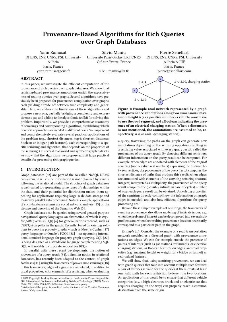
Figure 1: Example road network represented by a graph

with provenance annotations along two dimensions: max-

imum height ℎ (as a positive number) a vehicle must have

to use the road segment, and a Boolean indicating the pres-

ence of an electrical charging station. When a dimension

is not mentioned, the annotations are assumed to be, re-

spectively, ℎ ⩽ ∞ and ¬(charging station).

a query, traversing the paths on the graph can generate new

annotations depending on the semiring operators, resulting in

a semiring value associated with every query result, called the

provenance of the query result. By choosing different semirings,

different information on the query result can be computed. For

example, when edges are annotated with elements of the tropicalsemiring (nonnegative real numbers) expressing the distance be-

tween vertices, the provenance of the query result computes the

shortest distance of paths that produce this result; when edges

are annotated with elements of the counting semiring (natural

integers) interpreted as multiplicity, the provenance of the query

result computes the (possibly infinite in case of cycles) number

of ways each query result can be obtained. Underlying properties

of the semiring directly control how the information on graph

edges is encoded, and also how efficient algorithms for query

processing are.

Beyond these simple examples of semirings, the framework of

semiring provenance also allows modeling of intricate issues, e.g.,

when the problem of interest can be decomposed into several sub-

problems andwhen the resulting provenance does not necessarily

correspond to a particular path in the graph.

Example 1.1. Consider the example of a road transportation

network modeled as a directed graph with provenance anno-

tations on edges. We can for example encode the presence of

points of interests (such as gas stations, restaurants, or electrical

charging stations) as Boolean features on edges, and road prop-

erties (e.g., maximal height or weight for a bridge or tunnel) as

real-valued features.

We will show that, using semiring provenance, we can deal

with graph queries that take into account multiple such features:

a pair of vertices is valid for the queries if there exists at least

one valid path for each restriction between the two locations.

An application of this would be to ensure that different vehicle

categories (say, a high-clearance truck and an electric car that

requires charging on the way) can properly reach a common

destination from the same origin.

Another possible semantics for semiring provenance is to

check that all paths between two vertices verify (or exclude) some

properties (e.g., absence of tolls, or presence of gas stations on

the route) thus providing road administrators crucial information

on the global state of the roads between two points.

This is illustrated in Figure 1, a road network where some road

segments have restrictions on the height on vehicles; this is a

first dimension of provenance. The second dimension records

whether there exists an electrical charging station on the road

segment – in our example, this is the case for only one edge.

In our previous preliminary research [31], we generalized

three existing algorithms from a broad range of the computer

science literature to compute the provenance of regular path

queries over graph databases, in the framework of provenance

semirings. Together, these three generalizations cover a large

class of semirings used for provenance, each yielding a trade-

off between time complexity and generality. We also performed

experiments suggesting these approaches are complementary

and practical for various kinds of provenance indications, even

on a relatively large transport network.

In this paper, we extend this work by:

• Introducing a novel algorithm,MultiDijkstra, for com-

mutative 0-closed (or absorptive) semirings. This algorithm,

generalizing Dijkstra’s algorithm and leveraging prop-

erties of distributive lattices, partially bridges a strong

computational gap between two classes of semirings left

untreated in our previous research. The complexity of the

queries exemplified here belongs in this gap, and strongly

motivated our interest to develop the algorithms in this pa-

per. The experiments we performed demonstrate that our

new algorithm can scale up to very large networks with

dozens of millions of nodes, bringing a notable improve-

ment with respect to the state of the art of provenance

computation in graph databases.

• Establishing a precise summary, in the form of a taxonomy,

of the algorithms used in our context, along with their

complexities and expected properties of the underlying

semirings used for the provenance annotations. We also

analyze similarities with classes of semirings which are

used either for computing provenance of relational algebra

queries [19] or of Datalog programs [11].

• Performing a comprehensive set of experiments on real-

world data demonstrating the running time of provenance

computation over graphs, over a wide variety of semirings

and covering different use cases. We also observe that pa-

rameters depending on the topology of the graph, such as

treewidth [27] seem to have a higher impact on the effi-

ciency of the algorithm than distance-based parameters

such as the highway dimension [4]. The implementation of

all algorithms we use for these experiments is freely avail-

able at https://bitbucket.org/smaniu/graph-provenance/

src/master/.

The paper is organized as follows. We start by introducing

in Section 2 some preliminaries: graph databases enhanced by

provenance annotations, a short overview of the algebraic theory

of semirings, and an explanation on which semiring can be used

for provenance annotations in a few selected practical applica-

tions. We revisit in Section 3 the algorithms we proposed in [31]

and discuss their limitations. Section 4 is a taxonomy summa-

rizing classes of semirings and associated algorithms for graph

provenance. In Section 5, we introduceMultiDijkstra and the

mathematical theory behind distributive lattices, whichMulti-

Dijkstra relies on. We present experimental results comparing

all algorithms in practice in Section 6 before discussing related

work in Section 7.

2 PRELIMINARIES

The framework we are considering is that of graph databases

enriched with semiring-based provenance annotations. We detail

here the notation and definitions we previously introduced in [31]

and extend it with some additional concepts. We also introduce

a large number of example semirings, to illustrate the generality

of the problem considered.

2.1 Semirings

The framework for provenance in relational databases introduced

by [18] uses the algebraic structure of semirings to encode meta-

information about tuples and query results. In what follows,

we present the basic notions needed for this paper; for further

details about the theory and applications of semirings, see [20]

and [18, 34] for their applications to provenance.

Definition 2.1 (Semiring). A semiring is an algebraic structure

(K, ⊕, ⊗, 0, 1) where K is some set, ⊕ and ⊗ are binary operators

over K, and 0 and 1 are elements of K, satisfying the following

axioms:

• (K, ⊕, 0) is a commutative monoid: (𝑎⊕𝑏) ⊕𝑐 = 𝑎⊕ (𝑏⊕𝑐),𝑎 ⊕ 𝑏 = 𝑏 ⊕ 𝑎, 𝑎 ⊕ 0 = 0 ⊕ 𝑎 = 𝑎;

• (K, ⊗, 1) is a monoid: (𝑎 ⊗ 𝑏) ⊗ 𝑐 = 𝑎 ⊗ (𝑏 ⊗ 𝑐), 1 ⊗ 𝑎 =

𝑎 ⊗ 1 = 𝑎;

• ⊗ distributes over ⊕: 𝑎 ⊗ (𝑏 ⊕ 𝑐) = (𝑎 ⊗ 𝑏) ⊕ (𝑎 ⊗ 𝑐);• 0 is annihilator for ⊗: 0 ⊗ 𝑎 = 𝑎 ⊗ 0 = 0.

Example 2.2. It is easy to check that the following structures

are all semirings:

Tropical semiring. (R+ ∪ {∞},min, +,∞, 0).Top-𝑘 semiring. For 𝑘 ⩾ 1 some integer,

((R+ ∪ {∞})𝑘 ,min𝑘 , +𝑘 , (∞, . . . ,∞), (0,∞, . . . ,∞)),

where

min𝑘 ((𝑎1, . . . , 𝑎𝑘 ), (𝑏1, . . . , 𝑏𝑘 )) = min

𝑘 {𝑎1, . . . , 𝑎𝑘 , 𝑏1, . . . , 𝑏𝑘 }

returns the 𝑘 smallest entries (with duplicates) among

those in 𝑎 and 𝑏, in increasing order, and

(𝑎1, . . . , 𝑎𝑘 ) +𝑘 (𝑏1, . . . , 𝑏𝑘 ) = min𝑘 {𝑎𝑖 + 𝑏 𝑗 | 1 ⩽ 𝑖, 𝑗 ⩽ 𝑘}.

We further impose that only tuples that are in increasing

order are valid elements of the semiring. Note that the

top-1 semiring is the same as the tropical semiring.

Example: For 𝑘 = 2, (1, 2) ⊕ (1, 3) = min2{1, 1, 2, 3} = (1, 1)

and (1, 2) ⊗ (1, 3) = min2{1 + 1, 1 + 3, 2 + 1, 2 + 3} = (2, 3).

Counting semiring. (N ∪ {∞}, +,×, 0, 1), where

∀𝑎 ∈ N∗ 𝑎 + ∞ = 𝑎 ×∞ = ∞× 𝑎 = ∞

and 0 + ∞ = ∞, but 0 ×∞ = ∞× 0 = 0.

Boolean semiring. ({⊥,⊤},∨,∧,⊥,⊤), where ⊥ (resp, ⊤)is interpreted as the Boolean false (resp., true) value.

𝑘-feature semiring. For 𝑘 ⩾ 1 some integer,

((R+)𝑘 ,min,max, (∞,∞,∞), (0, 0, 0))

where min and max are applied pointwise; it also exists

in dual form, with min and max exchanged.

Integer polynomial semiring. (N[𝑋 ], +,×, 0, 1) where 𝑋is a finite set of variables, and +, ×, 0, 1 have their standardinterpretations as polynomial operators and polynomial

values.

Shortest-path semiring.

((R+ ∪ {∞}) × Σ∗, ⊕, ⊗, (∞, Y), (0, Y))with the following operators ⊕ and ⊗:• (𝑑, 𝜋) ⊕ (𝑑 ′, 𝜋 ′) = (min(𝑑,𝑑 ′), 𝜋 ′′) where 𝜋 ′′ is 𝜋 if

𝑑 < 𝑑 ′, 𝜋 ′ if 𝑑 > 𝑑 ′, and min(𝜋, 𝜋 ′) (in lexicographic

order, assuming some order on Σ) if 𝑑 = 𝑑 ′;• (𝑑, 𝜋) ⊗ (𝑑 ′, 𝜋 ′) = (𝑑 +𝑑 ′, 𝜋 ·𝜋 ′) if neither 𝑑 nor 𝑑 ′ is∞;and (𝑑, 𝜋) ⊗ (𝑑 ′, 𝜋 ′) = (∞, Y) if either 𝑑 or 𝑑 ′ is∞.

As we shall see further, these examples all yield useful appli-

cations for provenance over graphs.

We now consider properties of semirings that will be of interest

to develop specific algorithms – we will illustrate these properties

on the example semirings of Example 2.2. Some of the properties

are summarized in Figure 2; ignore annotations for algorithms

in blue for now.

A semiring is commutative if for all 𝑎, 𝑏 ∈ K, 𝑎 ⊗ 𝑏 = 𝑏 ⊗ 𝑎.A semiring is idempotent if for all 𝑎 ∈ K, 𝑎 ⊕ 𝑎 = 𝑎. In an

idempotent semiring we can introduce a natural order defined by𝑎 ⊑ 𝑏 iff it exists 𝑐 ∈ K such that 𝑎 ⊕ 𝑐 = 𝑏.1 Note that this orderis compatible with the two binary operations of the semiring: for

all 𝑎, 𝑏, 𝑐 ∈ K, 𝑎 ⊑ 𝑏 implies 𝑎 ⊕ 𝑐 ⊑ 𝑏 ⊕ 𝑐 and 𝑎 ⊗ 𝑐 ⊑ 𝑏 ⊗ 𝑐 . Animportant property that we wish to use in our setting is that of

k-closedness [29], i.e., a semiring is 𝑘-closed if:

∀𝑎 ∈ K,𝑘+1⊕𝑖=0

𝑎𝑖 =

𝑘⊕𝑖=0

𝑎𝑖 .

Here, by 𝑎𝑖 we denote the repeated application of the ⊗ operation𝑖 times, i.e., 𝑎𝑖 = 𝑎 ⊗ 𝑎 ⊗ · · · ⊗ 𝑎︸ ︷︷ ︸

𝑖

. 0-closed semirings (i.e., those

in which ∀𝑎 ∈ K, 1 ⊕ 𝑎 = 1) have also been called absorptive,bounded, or simple depending on the literature. Note that any

0-closed semiring is idempotent (indeed, 𝑎 ⊕ 𝑎 = 𝑎 ⊗ (1 ⊕ 1) =𝑎 ⊗ 1 = 𝑎) and therefore admits a natural order.

Example 2.3. All semirings in Example 2.2 are commutative

except for the shortest-path semiring (indeed, concatenation is

not a commutative operation).

All of them are idempotent, except for the top-𝑘 , counting,

and integer polynomial semirings.

The natural order of the tropical semiring is the total order ⩾(note that this is the reverse of the standard order on R+ ∪ {∞}).

The tropical, Boolean, 𝑘-feature, and shortest-path semirings

are 0-closed. The top-𝑘 semiring is (𝑘 − 1)-closed. The countingand integer polynomial semirings are not 𝑘-closed for any 𝑘 .

Star semirings [14], also known as closed semirings, extendsemirings with a unary

∗operator, having the following property:

𝑎∗ = 1⊕ (𝑎 ⊗ 𝑎∗) = 1⊕ (𝑎∗ ⊗ 𝑎). Note that, in 0-closed semirings,

we necessarily have 𝑎∗ = 1. Similarly, in 𝑘-closed semirings, we

can define 𝑎∗ =⊕𝑘

𝑖=0 𝑎𝑖.

Example 2.4. As just mentioned, since the tropical, Boolean,

𝑘-feature, and shortest-path semirings are all 0-closed, we can

simply define in all of them 𝑎∗ = 1. Since the top-𝑘 semiring is

(𝑘 − 1)-closed, we can define 𝑎∗ with the formula 𝑎∗ =⊕𝑘

𝑖=0 𝑎𝑖.

1In general semirings, this defines a preorder; antisymmetry of this relation can be

shown when the semiring is idempotent.

In the counting semiring we can introduce a star operator

with: 0∗ = 1 and 𝑎∗ = ∞ for 𝑎 ≠ 0.

It is not possible to simply add a star operator to the integer

polynomial semiring (indeed, if the equation 𝑥∗ = 1+(𝑥×𝑥∗) hada solution 𝑥∗ as a polynomial in 𝑥 , its degree would be different

on the left- and right-hand sides of the equation). However, one

can define a more general semiring, that of formal power series, inwhich a star operator can be defined. See [18] for details on the

semiring of formal power series, which are not important here.

We will later use the fact that a 0-closed semiring which is

alsomultiplicatively idempotent (i.e., in which 𝑎 ⊗ 𝑎 = 𝑎 for every

𝑎) turns out to satisfy the axioms of bounded distributive lattices[8, Theorem 10].

Example 2.5. The only 0-closed semirings that are multiplica-

tively idempotent from Example 2.2 are the Boolean and𝑘-feature

semirings.

2.2 Graph databases with provenance

We now introduce the notion of provenance in graph databases.

Definition 2.6 (Graph Database). A graph database with prove-nance indication (𝑉 , 𝐸, _,𝑤) over some semiring (K, ⊕, ⊗, 0, 1) isan edge-labeled directed graph (𝑉 , 𝐸, _) together with a weightfunction𝑤 : 𝐸 → K.

Given an edge 𝑒 = (𝑢, 𝑣) ∈ 𝐸, we denote 𝑛[𝑒] = 𝑢 its destina-tion (or next) vertex, and 𝑝 [𝑒] = 𝑣 its origin (or previous vertex).

By analogy we write its weight 𝑤 [𝑒] instead of 𝑤 (𝑒). Given a

vertex 𝑣 ∈ 𝑉 , we denote by 𝐸 [𝑣] the set of edges having 𝑣 as

origin.

A path 𝜋 = 𝑒1𝑒2 · · · 𝑒𝑘 in 𝐺 is an element of 𝐸∗ with consecu-

tive edges: 𝑛[𝑒𝑖 ] = 𝑝 [𝑒𝑖+1] for 𝑖 = 1, . . . , 𝑘 − 1. We extend 𝑛 and 𝑝

to paths by setting 𝑝 [𝜋] B 𝑝 [𝑒1], and 𝑛[𝜋] B 𝑛[𝑒𝑘 ]. A cycle

is a path starting and ending at the same vertex: 𝑛[𝑐] = 𝑝 [𝑐].The weight function𝑤 can also be extended to paths by defining

the weight of a path as the result of the ⊗-multiplication of the

weights of its constituent edges: 𝑤 [𝜋] B𝑘⊗𝑖=1

𝑤 [𝑒𝑖 ]; this can in

fact be extended to any finite set of paths by𝑤 [{𝜋1, . . . , 𝜋𝑛}] B⊕𝑛𝑖=1𝑤 [𝜋𝑖 ]. For any two vertices 𝑥 and𝑦 of a graph𝐺 , we denote

by 𝑃𝑥𝑦 (𝐺) the set of paths from 𝑥 to 𝑦.

Definition 2.7 (Path Provenance). Let 𝐺 be a graph database

with provenance indication over some semiring K. The prove-nance between 𝑥 and 𝑦, for 𝑥 and 𝑦 two vertices of 𝐺 is defined

as the (possibly infinite) sum:

provK (𝐺) (𝑥,𝑦) B 𝑤[𝑃𝑥𝑦 (𝐺)

]=

⊕𝜋 ∈𝑃𝑥𝑦 (𝐺)

𝑤 [𝜋] .

Several problems can be defined based on this. Given two

vertices 𝑠 and 𝑡 , the single-pair provenance problem computes

the provenance between 𝑠 and 𝑡 . Given a vertex 𝑠 , the single-source provenance problem computes the provenance between

𝑠 and each vertex of the graph. Finally, the all-pairs provenanceproblem computes the provenance for all pairs of vertices.

A regular path query (RPQ) [6] defines a set of admissible paths

from some vertex 𝑠 through a regular language over edge labels.

The notion of single-source provenance can be generalized to that

of RPQ provenance in a straightforward manner, as we did in [31].

We also showed in [31] that computing such a provenance could

be reduced in polynomial time to the single-source provenance

problem; this works by constructing a product of the graph with

the automaton describing the language of the query. Note that

this construction can be done on-the-fly (avoiding generation of

inaccessible vertices) and that the size of the automaton is usually

quite small; thus, the overhead is usually affordable oven for large

graphs as showed experimentally in [31]. We will implicitly use

this reduction throughout the paper, meaning that we only need

to consider the single-source provenance problem in the rest of

the paper. Consequently, we will also ignore edge labels and see

a graph database as defined by its vertices, edges, and semiring

weights.

2.3 Semantics of path provenance

As defined, the provenance between two vertices in a graph data-

base is in fact a (possibly infinite) sum over the provenances of all

paths from the source vertex leading to the target vertex. As we

observed in [30], the only possible source of non-finiteness in the

sum is due to cycles in the graph, so that we only need to be able

to sum all the powers of a given semiring value. For this to be se-

mantically meaningful we need the semiring to be a star semiring,

and we additionally need the star operator to verify for all semir-

ing element 𝑎: 𝑎∗ =⊕∞

𝑛=0 𝑎𝑛for some well-behaved infinitary

sum operation

⊕(namely, associativity, and distributivity of ⊗

over this infinitary sum operator). This class of semirings is com-

monly known as countably complete star semirings, c-completestar semirings [24], or 𝜔-complete star semirings.

Example 2.8. All star semirings identified in Example 2.4 are,

indeed, c-complete star semirings. Note that, for 𝑘-closed semir-

ings, the infinitary sum

⊕∞𝑛=0 𝑎

𝑛is simply

⊕𝑘𝑛=0 𝑎

𝑛, and the

condition of being a c-complete star semiring is trivially satisfied

by our choice of star operator. In the remaining cases (counting

semiring, formal power series, formal language semiring) one

can verify that a well-behaved infinitary sum operation can be

introduced, and that it verifies 𝑎∗ =⊕∞

𝑛=0 𝑎𝑛.

We also pointed out in [30] that all-pairs graph provenance

is equivalent to the computation of the asteration of the matrix

corresponding to the graph representation with provenance tags

as cell-values. With all these definitions in place, we observe

that the semantics of provenance over specific semirings actually

corresponds to a various number of problems of interest. Remem-

ber that using the construction of [31] we can extend this to the

provenance of arbitrary RPQs.

Example 2.9. Let𝐺 be a graph database over some c-complete

star semiring K, and 𝑠 and 𝑡 fixed source and target vertices in𝐺 .

The provenance between 𝑠 and 𝑡 corresponds to the following

notions, depending on the semiring K:

Tropical semiring: length of shortest path between 𝑠 and 𝑡 .

Top-𝑘 semiring: lengths of𝑘 shortest paths between 𝑠 and 𝑡 .

Counting semiring: total number of paths between 𝑠 and 𝑡 ,

edge weights being interpreted as number of edges be-

tween two vertices.

Boolean semiring: existence of a path between 𝑠 and 𝑡 ,

depending on the existence of edges denoted by their

Boolean weights.

𝑘-feature semiring: minimum feature value along each di-

mension of all paths between 𝑠 and 𝑡 ; if min and max are

exchanged, maximum feature value along some path from

𝑠 to 𝑡 .

Formal power series: how-provenance, see [18].

Shortest-path semiring: pair formed of a length 𝑙 and path

label 𝜋 such that 𝜋 is the shortest path from 𝑠 to 𝑡 , of

length 𝑙 (if there are multiple shortest paths, 𝜋 is the first

in lexicographic order).

Example 2.10. Let us return to the example in Figure 1. We

model the charging station Boolean feature as an integer feature

by simply setting ⊤ = 1 and ⊥ = 0. We take the (max,min) defi-nition of the 𝑘-feature semiring where we compute the maximum

value of each feature among some path from origin to destination,

and we order heights in decreasing order (e.g., by taking their

inverse) so that a higher feature value means a (more restrictive)

lower height.

Consider two types of vehicles of interest that want to reach

the vertex 𝑡 from the vertex 𝑠: one has height between 3 and 4

meters, the second is a small (ℎ ⩽ 1.5) electric car that needs

at least one charging station on the road to 𝑡 . In the presence

of the edge from 𝑢 to 𝑣 , both of them can reach 𝑡 from 𝑠; with-

out that edge, only the electric car is able to. This is reflected

in the provenance: prov(𝐺) (𝑠, 𝑡) = (4, charging station) whileprov(𝐺\{(𝑢, 𝑣)})(𝑠, 𝑡) = (2.10, charging station).

3 EXISTING ALGORITHMS

We now provide a review of three algorithms to solve the single-

source provenance problem, also previously described in [31].

Each of these algorithms yields a different trade-off between time

complexity and applicability to various types of semirings, as

summarized in Table 1.

Algorithm 1 Dijkstra – single-source

Input: (𝐺 = (𝑉 , 𝐸,𝑤), 𝑠) a graph database with provenance in-

dication over K and the source 𝑠 .

Output: Array w representing the single-source provenance

from 𝑠 of the reachability query.

1: 𝑆 ← ∅2: w[𝑎] ← 0, ∀𝑎 ∈ 𝑉3: w[𝑠] ← 1

4: while 𝑆 ≠ 𝑉 do

5: Select 𝑎 ∉ 𝑆 with minimal w[𝑎]6: 𝑆 ← 𝑆 ∪ {𝑎}7: for each neighbor 𝑏 of 𝑎 not in 𝑆 do

8: w[𝑏] = w[𝑏] ⊕ (w[𝑎] ⊗𝑤 [𝑎𝑏])9: end for

10: end while

11: return w

Dijkstra. Dijskstra’s algorithm is generally used to solve

shortest-distance problems in directed graphs. However, as shown

also in [31], the algorithm readily generalizes to our semiring

context, by placing some restrictions on the semirings used. For

instance, the tropical semiring is exactly the semiring that allows

to compute the shortest distance, as in the original algorithm.

The general flow of the algorithm – using general semiring op-

erations – is outlined in Algorithm 1, and Table 1 indicates its

running time (in terms of the graph size and the costs of the

semiring operations ⊕ and ⊗). Dijkstra’s algorithm is known to

be a very efficient algorithm. However, this efficiency comes from

the fact that it uses a priority queue: once a value is extracted

from it, we know that it is the correct one – this allows us to only

visit each vertex in the graph once. This only works if we apply

Dijkstra to semirings which are 0-closed (or absorptive) and in

which an additional condition is satisfied: the natural order is a

total order [31].As we shall discuss later, there is a large complexity gap be-

tween Dijkstra on the one hand and the other two algorithms

Table 1: Required semiring properties and asymptotic complexity for each studied algorithm, where T• is the complexity

of the elementary semiring operation •. The last column assumes constant cost for all semiring operations.

Name Semiring property Time complexity (with semiring op.) Time complexity

MatrixAsteration star O(|𝑉 |T∗ + |𝑉 |3 (T⊕ + T⊗)) O(|𝑉 |3)NodeElimination c-complete star O(|𝑉 |T∗ + |𝑉 |3 (T⊕ + T⊗)) O(|𝑉 |3)Mohri 𝑘-closed Exponential Exponential

MultiDijkstra 0-closed ⊗-idempotent O (ℓ × (T⊕ |𝑉 | log |𝑉 | + |𝐸 | (T⊕ + T⊗))) O(ℓ × (|𝑉 | log |𝑉 | + |𝐸 |))Dijkstra 0-closed total ordered O(T⊕ |𝑉 | log |𝑉 | + |𝐸 | (T⊕ + T⊗)) O(|𝑉 | log |𝑉 | + |𝐸 |)

we discuss in this section – NodeElimination and Mohri –

on the other. This is the main motivation to introduce the new

algorithm we present in Section 5.

Algorithm 2Mohri – single-source [29]

Input: (𝐺 = (𝑉 , 𝐸,𝑤), 𝑠) a graph database with provenance in-

dication over K and the source 𝑠 .

Output: Array w representing the single-source provenance

from 𝑠 of the reachability query.

1: for 𝑖 ∈ {1, . . . , |𝑄 |} do2: w[𝑖] ← 𝑟 [𝑖] ← 0

3: end for

4: w[𝑠] ← 𝑟 [𝑠] ← 1

5: 𝑆 ← {𝑠}6: while 𝑆 ≠ ∅ do7: 𝑞 ← head(𝑆)8: dequeue(𝑆)9: 𝑟 ′ ← 𝑟 [𝑞]10: 𝑟 [𝑞] ← 0

11: for each 𝑒 ∈ 𝐸 [𝑞] do12: if w[𝑛[𝑒]] ≠ w[𝑛[𝑒]] ⊕ (𝑟 ′ ⊗𝑤 [𝑒]) then13: w[𝑛[𝑒]] ← w[𝑛[𝑒]] ⊕ (𝑟 ′ ⊗𝑤 [𝑒])14: 𝑟 [𝑛[𝑒]] ← 𝑟 [𝑛[𝑒]] ⊕ (𝑟 ′ ⊗𝑤 [𝑒])15: if 𝑛[𝑒] ∉ 𝑆 then

16: enqueue(𝑆, 𝑛[𝑒])17: end if

18: end if

19: end for

20: end while

21: w[𝑠] ← 1

22: return w

Mohri. Mohri [29] introduced an algorithm for computing

single-source provenance for reachability queries over 𝑘-closed

semirings. Outlined in Algorithm 2, it performs, in a manner

similar to the Bellman–Ford algorithm, step-by-step relaxations

over the edges of the graph (lines 13–14), maintaining a queue to

decide in which order the elements are inspected. The queue can

be chosen in different ways: based on the topology of the graph,

e.g., if the graph is acyclic; or a queue prioritized by weight when,

e.g., one wishes to compute top-𝑘 shortest paths using the top-𝑘

semiring.

In the worst case, the theoretical complexity of this approach

is exponential in the size of the graph [29], mainly due to the fact

that the algorithm may have to visit the same cycle in the graph

multiple times. However, the complexity heavily depends on the

implementation of the queue. For instance, for top-𝑘 shortest

paths, implementing a priority queue allows for an efficient algo-

rithm, having polynomial complexity. Indeed, as we shall detail

later, for road transportation networks and top-𝑘 shortest paths,

experiments show an almost linear-time behavior in 𝑘 and the

size of the graph.

In contrast, the algorithm may be much more inefficient in

practice for other types of networks (such as social networks). As

we conjecture in Section 6, this may be due to the fact that trans-

port networks have relatively low treewidth [27]. The treewidth

is a parameter measuring how much a graph (or more gener-

ally any relational instance) resembles a tree. Many intractable

problems over graphs have tractable solutions on instances of

fixed treewidth. We confirm in Section 6 that many of the algo-

rithms for provenance computation strongly benefit – in terms

of running time – from low treewidth.

Another important graph parameter – stemming from the

active research community around computing routing for, e.g,

driving directions – the highway dimension [4] has been intro-

duced to provide a theoretical basis for the efficiency observed

in practice in state-of-the-art heuristics for computing optimal

transport paths. This parameter relies heavily on weights on the

edges of the graphs and the distribution of shortest distances in

the graph. In our experiments in Section 6, we evaluate whether

this parameter also explains the practical efficiency of our algo-

rithms for computing the provenance of routing queries.

Algorithm 3 NodeElimination – single-pair

Input: (𝐺 = (𝑉 , 𝐸,𝑤), 𝑠, 𝑡) a graph database with provenance

indication over K, the source 𝑠 , and the target 𝑡 .

Output: Single value w𝑠′𝑡 ′ representing the single-pair prove-

nance between 𝑠 and 𝑡 of the reachability query.

1: 𝑉 ′ ← 𝑉 ∪ {𝑠 ′, 𝑡 ′}2: 𝐸 ′ ← 𝐸 ∪ {(𝑠 ′, 𝑠), (𝑡, 𝑡 ′)}3: for 𝑖 ∈ 𝑉 ′ do4: for 𝑗 ∈ 𝑉 ′ do

5: w(0)𝑖 𝑗←

{𝑤 [𝑖 𝑗] if 𝑖 ≠ 𝑗,

1 ⊕ 𝑤 [𝑖 𝑗] if 𝑖 = 𝑗

6: end for

7: end for

8: for 𝑘 in 𝑉 do

9: for each (𝑝, 𝑞) s.t. (𝑝, 𝑘), (𝑘, 𝑞) ∈ 𝐸 ′ do10: w𝑝𝑞 ← w𝑝𝑞 ⊕

(w𝑝𝑘 ⊗ w

∗𝑘𝑘⊗ w𝑘𝑞

)11: end for

12: end for

13: return w𝑠′𝑡 ′

NodeElimination. The most general algorithm available is

based on the idea of Brzozowski and McCluskey for obtaining a

formal language expression (i.e., a regular expression) equivalent

to the language of an automaton [9]. The algorithm is outlined

in Algorithm 3. The algorithm works by eliminating vertices one

by one and computing the “shortcut” values for each vertex pair,

until only the source and target vertices remain. This algorithm

works for any 𝑐-complete semiring over which a star operationis defined – this is necessary for the shortcuts computed in the

algorithm to be correct.

0-closed

total order

Dijkstra

0-closed⊗-idemp.

MultiDijkstra

0-closed

𝑘-closed

Mohri

c-complete star semirings

NodeElimination

star semirings

MatrixAsteration

semirings

Figure 2: Taxonomy of the semirings used for graph provenance along with algorithms that work on them

In general, the complexity of the algorithm is at least cubic in

the number of vertices in the graph, which makes it practically

unusable on large graphs. Importantly, however, it also can be

shown that its complexity is closely related to the treewidth pa-

rameter of the graph. Following a simplicial elimination order

(unfortunately not tractable to compute) one can rephrase the

complexity shown in Table 1 in terms of the treewidth parame-

ter 𝑤 by O(|𝑉 |T∗ + |𝑉 |𝑤2 (T⊕ + T⊗)). Thus, if the treewidth is

small over, e.g., transportation networks, one can benefit from

heuristics for finding a suitable elimination order to optimize this

algorithm. We dedicate a part of our experiments demonstrating

the impact of some heuristics (for instance, focusing on vertices

of higher degrees) on the running time of this algorithm.

Related algorithms. Star semirings are also known as closed

semirings [2] and the star operation is known as the closure

operation. In this sense, all-pair computations correspond to

matrix asteration. For instance, the NodeElimination algorithm

can be used to compute the asteration [2] of a matrix – but, if the

semiring is not c-complete, there is no guarantee of a semantics

compatible with the intuitive semantics of provenance over graph

databases. Matrix asteration allows for a high degree of parallel

computation [1].

4 TAXONOMY

We present in Figure 2 a high-level view linking the properties

and classes of semiring we presented in Section 2 and their as-

sociated algorithms, presented in Sections 3 and 5. The figure

shows a clear hierarchy of classes of semirings, both in terms of

the complexity of the algorithm and the expressive power of the

semirings.

An important practical application that is similar to our setting

is the provenance for Datalog queries introduced in [18] and

further optimized using circuits [11]. Datalog [3] is a language

derived from Prolog, useful for infering new knowledge given

existing facts and a set of inference rules. In the papers above, the

semiring classes for which optimization of queries is possible are

strikingly similar: PosBool(𝑋 ) and Sorp(𝑋 ) discussed in [11, 18]

correspond respectively to the positive fragment of the Boolean

function semiring, and to the free (i.e., most general) 0-closed

semiring. In that sense, algorithm optimizations discussed here

apply directly to applications such as Datalog query optimization.

5 ALGORITHM FOR 0-CLOSED SEMIRINGS

As explained in Section 3, Dijkstra requires a total natural order

on the elements of a 0-closed semiring. This is quite a restrictive

setting (among the examples from Example 2.2, only the tropicalsemiring fits), while using a more generally available algorithm

such as Mohri can lead to practical inefficiency. The question

we are addressing in this section is whether we can bridge this

complexity gap and still obtain practical algorithms for 0-closed

semiring without total orders.

First, we present an example semiring setting, with non-total

natural order, where Dijkstra cannot be readily applied.

Example 5.1. Let us consider the 3-feature semiring

({0, 1}3,min,max, (1, 1, 1), (0, 0, 0)) .In the example graph below, the provenance between 𝑠 and 𝑡

is: min (max ((0, 0, 1), (0, 1, 0)) , (1, 0, 0)) = (0, 0, 0) and that be-

tween 𝑠 and 𝑟 is: min (max ((1, 0, 0), (0, 1, 0)) , (0, 0, 1)) = (0, 0, 0)

s

r

t

(0, 0, 1)

(0, 1, 0)

(1, 0, 0)

Assume there would be an order for whichDijkstra computes

this provenance. Then, starting from 𝑠 , Dijkstra would select

either 𝑟 and assign it provenance (0, 0, 1), which is wrong, or 𝑡

and assign it provenance (1, 0, 0), which is also wrong.

In the following, we address this problem and design a new

algorithm,MultiDijkstra (for Multidimensional Dijkstra) thatapplies to the more general case of 0-closed semirings for which

multiplication is idempotent (such as the 𝑘-feature semiring, but

also the Boolean function semiring used in probabilistic databases,

see [34]). As it turns out, such semirings satisfy the axioms of

bounded distributive lattices [8, Theorem 10]; this allows us to

design an efficient algorithm for answering queries using these

types of semirings.

5.1 Mathematical Background

In the following we introduce basic notions about finite distribu-

tive lattices. We assume the lattices we use are finite because

we are only ever using the subsemiring generated by edge an-

notations. As we shall see, this subsemiring is finite when both

operations of the semiring are idempotent.

We refer the reader to [36] for more details regarding the

theory behind distributive lattices.

5.1.1 Definitions and Notation. A lattice (𝐿, <) is a partiallyordered set (poset) where every two elements have a unique

infimum (their meet, ∧) and supremum (their join, ∨). A latticeembedding of a lattice 𝐿 into a lattice 𝐾 is a one-to-one join

and meet homomorphism from 𝐿 to 𝐾 . In a poset, an element 𝑦

covers 𝑥 (denoted 𝑥 ⋖ 𝑦) if 𝑥 < 𝑦 and there are no such 𝑧 such

that 𝑥 < 𝑧 < 𝑦. A lattice embedding ℓ is tight if 𝑥 ⋖ 𝑦 implies

ℓ (𝑥) ⋖ ℓ (𝑦).2An element 𝑥 of a lattice 𝐿 is join-irreducible if 𝑥 = 𝑎 ∨ 𝑏

implies that 𝑥 = 𝑎 or 𝑥 = 𝑏. The set of non-zero join-irreducible

elements of 𝐿 is denoted 𝐽 (𝐿). It induces a subposet of 𝐿 which

is also denoted by 𝐽 (𝐿).For a subset 𝑆 of a lattice 𝐿, we let

∨𝑆 =

∨𝑥 ∈𝑆 𝑥 be the join

of the elements of 𝑆 . We often write

∨𝐿 𝑆 to specify that the join

takes place in 𝐿. A subset 𝑆 of a poset is a downset or ideal if𝑥 ∈ 𝑆 and𝑦 ⩽ 𝑥 implies𝑦 ∈ 𝑆 . The minimum downset containing

an element 𝑥 is denoted id 𝑥 . We note D(𝑃), for a poset 𝑃 , thefamily of downsets of 𝑃 ordered by inclusion.

A chain 𝐶 of length 𝑛 in a poset 𝑃 is a subposet isomorphic to

the linear order Z𝑛 on the 𝑛 elements {0, 1, . . . , 𝑛 − 1}. A chaindecomposition of a poset 𝑃 is a partition of its elements into a

family C of chains 𝐶1, . . . ,𝐶𝑑 . For a family C = {𝐶1, . . . ,𝐶𝑑 }

of disjoint chains, the product

∏C :=𝑑∏𝑖=1𝐶𝑖 consists of all 𝑑-

tuples 𝑥 = (𝑥1, . . . , 𝑥𝑑 ) where 𝑥𝑖 ∈ 𝐶𝑖 for each 𝑖 ∈ {1, . . . , 𝑑}. It isordered by 𝑥 ⩽ 𝑦 if 𝑥𝑖 ⩽ 𝑦𝑖 for each 𝑖 .

5.1.2 Results. A classical result from Birkhoff [7] establishes

an isomorphism between 𝐿 and D(𝐽 (𝐿)):

Theorem 5.2 ([7]). The map S : 𝑥 ↦→ id 𝑥 ∩ 𝐽 (𝐿) is an isomor-phism of 𝐿 to D(𝐽 (𝐿)). Its inverse is 𝑆 ↦→ ∨

𝐿 𝑆 .

For a chain decomposition C of a poset, let C0 be the family of

chains we get from the chains in C by adding a new minimum el-

ement to each. In [12], Dilworth proved the following embedding

theorem:

Theorem 5.3 ([12]). For any chain decomposition C of a poset 𝑃the map 𝑆 ↦→ ∨

𝑃 𝑆 is an embedding of D(𝑃) into 𝑃 =∏C0.

Then, we obtain the following corollary we will use later:

Corollary 5.4. Given a chain decomposition C of a distributivelattice 𝐿, there is a tight embedding of 𝐿 into

∏C0.5.2 Application to Provenance Computation

Corollary 5.4 provides us with a way to compute provenance

over distributive lattices using a multidimensional version of

Dijkstra’s algorithm. Because an embedding is a homomorphism,

we can compute each component of

∏C0 independently. Andbecause the homomorphism is one-to-one, we can easily recover

the provenance at the end of the computation.

Example 5.5. If we take a look at distributive lattice of the

divisors of 60 with greatest common divisor (gcd) and least

common multiple (lcm) as join and meet operators, we notice

that the divisors of 60 are either powers of 2, 3, 5 or an lcm

2Implicitly from lattice notation to poset notation: 𝑥 ∨ 𝑦 = 𝑦 means 𝑥 ⩽ 𝑦.

of these integers. Thus, they can be represented using three di-

mensions representing the factorization of 60 along these prime

numbers: decompose(4) = (2, 0, 0), recompose(0, 1, 0) = 3, and

recompose(2, 1, 0) = 12. We can then compute independently each

dimension of the result using Dijkstra’s algorithm since each

component is totally ordered; then, partial results are combined.

In other words, we can run separately, ℓ times, Dijkstra’s algo-

rithm for each dimension of this product, where ℓ is the number

of chains in the chain decomposition. This gives us a parameter-

ized algorithm, where ℓ depends on the semiring. For example, for

the semiring used in Example 5.1, ℓ = 3. We outline the algorithm

in pseudo-code in Algorithm 4. We need the following routines

that are highly specific to the semiring: decompose(𝑒) takes asparameter an element 𝑒 of 𝐿 and returns its image 𝑣 (𝑒) ∈ P. Forthe opposite direction recompose(𝑑1, . . . , 𝑑𝑛) =

∨0⩽𝑖⩽𝑛 𝑑𝑖 returns

as expected an element of 𝐿.

We use as a subroutine a slightly modified version of Dijk-

stra, parameterized by the semiring dimension and working

with semirings having elements in vector form, corresponding

to the decomposition. Dijkstra(s,t,i) ∈ 𝐽 (𝐿) computes the prove-

nance between 𝑠 and 𝑡 corresponding to the 𝑖th dimension of the

decomposition.

Example 5.6. We describe the working of Algorithm 4 in the

example presented in Example 5.1: first, each edge value is de-

composed; this step is easy to follow as the 3-feature values

are already presented in decomposed form. A second step con-

sists in calculating values along each dimensions. Algorithm 1

is launched a first time over the graph with edge values corre-

sponding to the first dimension: 0 for (𝑠, 𝑟 ) and (𝑟, 𝑡), 1 for (𝑠, 𝑡).The result is 0. Algorithm 1 is launched a second time over the

graph with edge values corresponding to the second dimension:

0 for (𝑠, 𝑟 ) and (𝑠, 𝑡), 1 for (𝑟, 𝑡). The result is, again, 0. Finally,Algorithm 1 is launched a third time over the graph with edge

values corresponding to the third dimension: 0 for (𝑠, 𝑡), 1 for

(𝑠, 𝑟 ) and (𝑟, 𝑡). The result is 0. This ends the second step. The

third step consists in recomposing partial values obtained by

successive applications of Dijkstra’s algorithm. This ends up to

the final provenance value of (0, 0, 0).

Algorithm 4 MultiDijkstra – single-pair

Input: (𝐺 = (𝑉 , 𝐸,𝑤), 𝑠, 𝑡) a graph database with provenance

indication over K, the source 𝑠 , and the target 𝑡 .

Output: Single-pair provenance of the reachability query from 𝑠

to 𝑡 .

1: for each edge 𝑒 ∈ 𝐸 do

2: decompose(𝑤 (𝑒))3: end for

4: for each dimension 𝑖 do

5: 𝑑𝑖 ← Dijkstra(𝑠, 𝑡, 𝑖)6: end for

7: return recompose(𝑑1, . . . , 𝑑𝑛)

For the sake of simplicity, we presented the single-pair version

of our algorithm. To extend it to the single-source version one

only needs to perform the recompose subroutine for each vertex

in the graph.

To minimize accesses to the decompose subroutine – which

can be very costly – we optimize MultiDijkstra by adopting

a lazy approach, where the Dijkstra subroutine calls decomposeonly when needed, storing the decomposition across calls. This

avoids scanning the whole graph when 𝑠 and 𝑡 are close.

Rome99, original Rome99, random Rome99, same USPowerGrid, random Yeast, random Stif, random

0.001

0.01

0.1

1

10

100

1 000

time(s)

BFS Dijkstra (Tropical) Mohri (Tropical) Mohri (Top-k) NodeElimination-Degree (Tropical)

Figure 3: Comparison between algorithms for shortest distances

Table 2: Graph datasets: size and treewidth lower and up-

per estimates from [27]

type name # of vertices # of edges tw

infrastructure Paris 4 325 486 5 395 531 55–521

Stif 17 720 31 799 28–86

USPowerGrid 4 941 6 594 10–18

Rome99 3 353 4 831 5–50

social Facebook 4 039 88 234 142–237

biology Yeast 2 284 6 646 54–255

Two other optimizations implemented are a stopping condi-

tion that ends the Dijkstra subroutine when a visited vertex has

value 0, and lazy initialization of the priority queue. These two

optimizations led to vastly improved computation times over the

naive implementation.

5.3 Practical Use Case

As exemplified in the Introduction, 𝑘-feature semirings can be

used to ensure that all paths from 𝑠 to 𝑡 verify a combination of

features (they all go through a specific set of points of interests,

or verify some road properties) or either ensure the existence

of valid paths up to some collection of restrictions. We show in

the experimental section that this is tractable for practical use

cases (continental-sized areas, around 107vertices). To the best

of our knowledge, no solution for this that scales even to graphs

of thousands of vertices has been previously proposed.

6 EXPERIMENTS

We performed experiments on real-world graph data, using an

Inria computing cluster running the OAR task manager. The

individual vertices of the cluster have a minimum of 48 GB of

RAM, and run Intel Xeon X5650 or E5-26xx CPUs.

We used datasets3from a variety of domains, mostly repre-

senting infrastructure networks: the OpenStreetMaps network

of Paris (Paris), the Paris public transport network (Stif), and

3These datasets were used in [27] for treewidth computation experiments, and are

downloadable from https://github.com/smaniu/treewidth/; some of them originate

from http://snap.stanford.edu/data/index.html.

the power grid of the continental US (USPowerGrid). For com-

parison, we have also evaluated on other types of datasets: a

small subset of the Facebook social network (Facebook) and

the yeast protein-to-protein interaction network (Yeast). All

these datasets come without provenance annotations, that we

add in different ways depending on experiments. We also used

a real weighted road transportation network dataset Rome99,

with tropical semiring annotations, from the 9th DIMACS Imple-

mentation Challenge4. This dataset consists of a large portion of

the directed road network of the city of Rome, Italy, from 1999.

Basic information about the resulting graphs are summarized in

Table 2.

For datasets without provenance annotations, unless speci-

fied differently, we randomly generate weights in the tropical

semiring for benchmarks, uniformly between 1 and 3 000. To be

able to compare the impact of the weights on the performance

of the algorithms, we also use a constant-weight setting, where

all weights equal to 1. Each experiment generally represents the

average over 10 runs (random choices of origin and destination

vertices).

Our experimental study is focused on comparing the four algo-

rithms presented in this paper, over several semirings.We provide

a comparison of all of our algorithms for the computation over

the tropical semiring (shortest distance), since all algorithms can

be used in this setting. We investigate the running time and the

number of relaxation steps performed byMohri andMultiDi-

jkstra algorithm, using initial weights provided by the dataset

Rome99, as well as custom weights (all identical and all random);

we then study over all datasets the impact of the elimination or-

der heuristic on the overall performance for NodeElimination.

We then finish with the comparison between our new algorithm

and previous solutions to demonstrate its efficiency.

Evaluating shortest distances. We start by evaluating how the

algorithms deal with the shortest distance semiring, i.e., the trop-

ical and top-𝑘 semiring (by setting 𝑘 = 1). The properties of this

semiring allow their implementation for the first three algorithms:

4http://users.diag.uniroma1.it/challenge9/download.shtml

0 5 10 15 20 25 30 35 40 45 50 55 60 65 70 75 80 85 90 95 100

0

0.5

1

1.5

2

2.5

3

3.5

4

4.5

k

time(s)

Mohri, original

Mohri, random

Mohri, same

Figure 4: Computation time for Mohri over the top-𝑘 distances semiring, for varying values of 𝑘 and varying weight

assignments (Rome99)

0 5 10 15 20 25 30 35 40 45 50 55 60 65 70 75 80 85 90 95 100

0

1

2

3

4

5

6

7

8

9

10

11

12

13

14

15

16

17

k

nbofrelaxationsperformed(×1

04)

Mohri, original

Mohri, random

Mohri, same

Figure 5: Number of relaxations performed byMohri over the top-𝑘 distances semiring, for varying values of𝑘 and varying

weight assignments (Rome99)

Rome99, original Rome99, random Rome99, same USPowerGrid, random Yeast, random Facebook, random Stif, random Paris, random

10

100

1 000

10 000

100 000

6.8 · 101 6.8 · 101 6.8 · 101

4.2 · 102

1.4 · 103

9.3 · 103

3.1 · 101 3 · 101 3.1 · 101

1.2 · 1012 · 101

1.2 · 1031 · 103

time(s)

NodeElimination (Id) NodeElimination (Degree)

Figure 6: Comparison between elimination orders for NodeElimination algorithm (tropical semiring). Values greater

than 100 000 s are timeouts.

Dijkstra, Mohri, and NodeElimination, whereas MultiDijk-

stra reduces to Dijkstra in that case. We also implemented a

breadth-first-search traversal for computing accessibility with

no provenance information (BFS). This also allows us to com-

pare the performance of algorithms against non-annotated graph

databases.

Rome99, random USPowerGrid, random Stif, random

0.001

0.01

0.1

1

10

100

1 000

4.2 · 1011.4 · 101

1.5 · 103

2.2 · 10−31.1 · 10−3

3.9 · 10−2

6.3 · 10−4 7.2 · 10−4

2.9 · 10−2

time(s)

NodeElimination (Degree) Mohri MultiDijkstra

Figure 7: Comparison between NodeElimination,Mohri, andMultiDijkstra (3-feature semiring)

1 2 3 4 5 6

10−3

10−1

101

103

number of features

time(s)

Mohri, 5 values

Mohri, 4 values

Mohri, 3 values

MultiDijkstra, 5 values

MultiDijkstra, 4 values

MultiDijkstra, 3 values

Figure 8: Computation time forMohri andMultiDijkstra depending on the number of dimensions (Rome99)

104

105

106

107

10−3

10−2

10−1

100

101

number of nodes

time(s)

Mohri

MultiDijkstra

Figure 9: Average computation time for Mohri and MultiDijkstra over random graphs depending on the number of

nodes; shaded areas indicate minimum and maximum computation times observed (3-feature semiring)

Figure 3 shows, on a logarithmic scale, the result for our graphs,

and for some settings of weights (original, random, or same

weights). It is immediately clear from the figure that the choice

of algorithm is crucial: we need the most specialized algorithm

for the semiring we use: Dijkstra is more efficient than Mohri

which is more efficient than NodeElimination. Even forMohri,

we notice that using it configured for the top-𝑘 semiring with

𝑘 = 1 does introduce an overhead in execution; when using the

tropical semiring directly the overhead is smaller. We also show

the overhead introduced when using provenance annotations

is quite limited, as the difference between Dijkstra and BFS is

less than an order of magnitude for each dataset, and Dijkstra

sometimes even outperforms BFS. Finally, NodeElimination is

always several orders of magnitude slower than Dijkstra. Another

encouraging result is that Mohri – which allows more classes

of semirings than Dijkstra – has a reasonable running time in

practice, despite the stated exponential complexity bound in the

original paper. We turn to evaluating its performance next.

Mohri in practice. In Figure 4 and in Figure 5 we respectively

study the impact of the factor 𝑘 on the running time and on the

number of computations performed by the algorithm. Our results

show that the computational time is linear in 𝑘 , though this is

not the case for the number of relaxations, which increases sub-

linearly in 𝑘 . This means that for large values of 𝑘 the algorithm

spends most of its time maintaining the queue.

We also compare the performance of the algorithm depending

on weight assignment (original, random, same). It seems that

considering random values instead of “real” values has almost no

significant impact over the efficiency of the algorithm. This is a

somewhat disappointing result because it rules out the possibility

to parametrize the complexity of the algorithm through network

parameters, for instance, in terms of the highway dimension [4] –

a graph parameter that has been successfully applied for under-

standing the efficiency of state-of-the-art shortest-distance algo-

rithms in road networks. However, the performance increases sig-

nificantly when all weights are uniform, which may be expected

since computation of shortest distances become far simpler, and

far more paths have equal distance.

As pointed out in Section 3 this algorithm performs extremely

well over transportation networks. We wanted to provide a com-

parison of its working time for different kinds of graphs (es-

pecially graphs whose treewidth is large relative to their size).

For this purpose we used a social network dataset: who-trusts-

whom network of people who trade using Bitcoin on a platform

called Bitcoin Alpha [25, 26] (3 783 vertices and 24 186 edges).

The algorithm times out after 48 hours.

What we can learn from this is that the key property making

Mohri so efficient over transportation networks is not due to

distance properties (e.g., highway dimension) – impacted by the

weights of the connections – but rather by topological properties

of the underlying graph (e.g., treewidth).

Ordering for NodeElimination. NodeElimination’s perfo-mance, due to its main loop of creating “shortcuts” in the graph,

is heavily dependent on the order in which the vertices are

eliminated. This elimination ordering is strongly linked to the

treewidth parameter of the graph. For instance, following a degree

based elimination order gives an upper bound on this parameter.

Hence, we have compared different elimination orders for

NodeElimination and found out that the minimum degree based

elimination order (Degree) greatly improves the efficiency of

this algorithm compared to having no such heuristic (Id). Thisimprovement can be dramatic, as for the Yeast dataset where the

algorithm is two orders of magnitude faster. As expected, weights

over the edges doesn’t impact the running time, as shown in

Figure 6.

This is important in practice: running NodeElimination on

low-treewidth graphs (e.g., infrastructure and transport networks)

can be the difference between the algorithm being unusable and

allowing reasonable running times. Taking into account that

NodeElimination allows for a large class of semirings, this can

have a significant real-world application impact.

MultiDijkstra. We now evaluateMultiDijkstra, our con-

tribution to bridging the gap between absorptive semirings and

more general ones. We compare it to Mohri and NodeElimina-

tion in the case of the 𝑘-feature semiring, which is kind of the

canonical semiring that is 0-closed and multiplicatively idem-

potent. Figure 7 showcases this on 3 datasets. In all cases, our

new algorithm is between 3 and 4 orders of magnitude faster

than NodeElimination, depending on the network we use, and

significantly faster thanMohri.

We then performed an additional experiment (Figure 8), exam-

ining the impact of the number of features and values actually

used in each feature on the running time of both algorithms. We

found out that when either one of the two criteria reaches 4,

Mohri times out while MultiDijkstra keeps scaling.

Finally, Figure 9 presents a comparison betweenMohri and

MultiDijkstra on large Erdős–Rényi random generated graphs

(generated using Python networkx’s fast_gnp_generationmethod,

using an average of 1.7 edges per vertex) show that our new

algorithm is still tractable for continental-sized graphs of millions

of vertices. Interestingly,MultiDijkstra also exhibits a much

smaller variance than that of Mohri, whose performance varies

by more than one order of magnitude between runs.

7 RELATEDWORK

The idea of encapsulating operations carried along by graph algo-

rithms in terms of semirings has been really common for decades.

In [10, Chapter 25] the authors presented two of the classical

graph algorithms, Floyd–Warshall and transitive closure algo-

rithm in terms of closed semirings. The APSP (All-Pairs Shortest-Path problem) is elegantly expressible using star semirings; hence,

research focused on the links to linear algebra through matrix

computations [1], allowing to speed up the response time using

parallel computations. Recent work on semiring-based graph

processing has provided to the community some tools such as

GraphBLAS [23], a library of kernel functions dedicated to opti-

mize linear algebra computations over sparse matrices. Unfortu-

nately, this tool focuses essentially on matrix and vector products

and is not amenable to express priority queue management such

as those needed for Mohri, Dijkstra, MultiDijkstra. Only

NodeElimination and the matrix asteration algorithms could

benefit of a GraphBLAS implementation: this might increase

their performance, even when retaining their higher asymptotic

complexity with respect to other algorithms.

Amongst many other fields, semirings have been successfully

applied in constraint-solving programming [8], linguistic struc-

ture prediction [37] and formal language theory [33]. This alge-

braic structure is also perfectly suited to the modeling of dynamic

programming [21].

The notion of provenance has also been initially developed

using semirings [18], either for relational databases and Datalog

programs, leading to practical systems such as [35], an exten-

sion to PostgreSQL adding the support for provenance. Many

representation frameworks have been successfully applied to

speed up the computation of the provenance for Datalog pro-

grams, most notably a circuit-based provenance approaches [11]

and the solving of fixed-point equations using derivation tree

analysis [15]. The latter approach led to a proof-of-concept im-

plementation [16] of the resolution of fixed-point equations over

c-continuous semirings using the Newton method.

Compared to our work, relational databases lack the effective

support for navigational queries (recursion is an issue) and Data-

log programs are much more expressive than graphs (they are

closely related to hypergraphs), so we suspect query answering

in Datalog would be highly inefficient for the continental-sized

road-network datasets we target, though we leave this investiga-

tion for future work.

Numerous notions of provenance co-exist in the literature and

each target different usages. The notion we use in this paper

considers the provenance to be computational rather than just in-

formational: we can apply operations over our provenance values

with different semantics depending on the underlying semiring.

Some practical systems, such as [28] rely on property graphs to

represent provenance annotations, that are of an informational

rather than computational nature. Those systems focus on the

further querying of obtained provenance to derive additional

information about the process.

8 CONCLUSIONS

We presented in this paper a study on evaluating the provenance

of rich graph queries using the semiring provenance framework.

We established a taxonomy of semiring classes, based on their

properties. This in turn allows us to find, for a set of impor-

tant semiring classes, the most appropriate algorithm, enabling

real-world applicability. We introduce a new algorithm,MultiDi-

jkstra, which bridges the gap between algorithms for absorptive

semirings and ones for more general classes.

Experimentally, on graph datasets from various domains, we

showed that making sure that the appropriate algorithm is chosen

for the semiring specialization is crucial; gains of several orders of

magnitude are observed between algorithms on the same graph

datasets. Moreover, we notice that algorithms for which their

theoretical complexity is high perform well in practice, especially

on graphs having relatively low treewidth.

We believe the link with classes of semiring for which an

optimization for the computation of the provenance for Datalog

queries exists is a key observation for optimizing computations

in our framework. Investigating this further will allows us to

benefit from the rich literature around Datalog provenance (in

particular, [11]) and to compare to our solutions.

ACKNOWLEDGMENTS

This work has been funded by the French government under

management of Agence Nationale de la Recherche as part of the

“Investissements d’avenir” program, reference ANR-19-P3IA-0001

(PRAIRIE 3IA Institute).

REFERENCES

[1] S. Kamal Abdali. 1994. Parallel Computations in *-Semirings. In ComputationalAlgebra, Klaus G. Fischer, Philippe Loustaunau, Jay Shapiro, Edward L. Green,

and Daniel Farkas (Eds.). Taylor & Francis, Chapter 1, 1–16.

[2] S. Kamal Abdali and David Saunders. 1985. Transitive closure and related

semiring properties via eliminants. Theoretical Computer Science 40 (1985),257–274. https://doi.org/10.1016/0304-3975(85)90170-7

[3] Serge Abiteboul, Richard Hull, and Victor Vianu. 1995. Foundations ofDatabases. Addison Wesley.

[4] Ittai Abraham, Amos Fiat, Andrew V. Goldberg, and Renato Fonseca F. Wer-

neck. 2010. Highway Dimension, Shortest Paths, and Provably Efficient Algo-

rithms. In SODA. Society for Industrial and Applied Mathematics, Philadelphia,

PA, USA, 782–793. http://dl.acm.org/citation.cfm?id=1873601.1873665

[5] Marcelo Arenas and Jorge Pérez. 2011. Querying semantic web data with

SPARQL. In PODS. New York, 305–316.

[6] Pablo Barceló. 2013. Querying Graph Databases. In PODS. ACM, New York,

175–188.

[7] Garrett Birkhoff. 1937. Rings of sets. Duke Math. J. 3, 3 (1937), 443–454.

https://doi.org/10.1215/S0012-7094-37-00334-X

[8] Stefano Bistarelli, Ugo Montanari, and Francesca Rossi. 1997. Semiring-based

constraint satisfaction and optimization. J. ACM 44, 2 (1997), 201–236. https:

//doi.org/10.1145/256303.256306

[9] Janusz A. Brzozowski and Edward J. McCluskey. 1963. Signal Flow Graph

Techniques for Sequential Circuit State Diagrams. IEEE Trans. Electr. Comp.EC-12, 2 (1963), 67–76.

[10] Thomas H. Cormen, Charles E. Leiserson, Ronald L. Rivest, and Clifford Stein.

2001. Introduction to Algorithms (2nd ed.). The MIT Press.

[11] Daniel Deutch, Tova Milo, Sudeepa Roy, and Val Tannen. 2014. Circuits for

Datalog Provenance. In ICDT. 201–212.[12] Robert P. Dilworth. 1950. A Decomposition Theorem for Partially Ordered

Sets. Annals of Mathematics 51, 1 (1950), 161–166. http://www.jstor.org/

stable/1969503

[13] Pedro Domingos and Matthew Richardson. 2001. Mining the network value

of customers. In KDD. ACM, New York, 57–66.

[14] Manfred Droste, Werner Kuich, and Heiko Vogler. 2009. Handbook of WeightedAutomata. Springer, Berlin.

[15] Javier Esparza and Michael Luttenberger. 2011. Solving fixed-point equa-

tions by derivation tree analysis. In International Conference on Algebra andCoalgebra in Computer Science. Springer, 19–35.

[16] Javier Esparza, Michael Luttenberger, and Maximilian Schlund. 2014. FP-

soLvE: A Generic Solver for Fixpoint Equations Over Semirings. Interna-tional Journal of Foundations of Computer Science 26. https://doi.org/10.1007/

978-3-319-08846-4_1

[17] Nadime Francis, Andrés Taylor, Alastair Green, Paolo Guagliardo, Leonid

Libkin, Tobias Lindaaker, Victor Marsault, Stefan Plantikow, Mats Rydberg,

and Petra Selmer. 2018. Cypher: An Evolving Query Language for Property

Graphs. In SIGMOD. 1433–1445. https://doi.org/10.1145/3183713.3190657

[18] Todd J. Green, Grigoris Karvounarakis, and Val Tannen. 2007. Provenance

Semirings. In PODS. ACM, New York, 31–40.

[19] Todd J. Green and Val Tannen. 2017. The Semiring Framework for Database

Provenance. In PODS. Association for Computing Machinery, New York, NY,

USA, 93–99. https://doi.org/10.1145/3034786.3056125

[20] Udo Hebisch and Hanns J. Weinert. 1998. Semirings: Algebraic Theory andApplications in Computer Science. World Scientific, Singapore.

[21] Liang Huang. 2008. Advanced Dynamic Programming in Semiring and Hy-

pergraph Frameworks. (2008), 18.

[22] ISO SC32 / WG3. [n.d.]. Graph Query Language GQL. https://www.

gqlstandards.org/.

[23] J. Kepner, P. Aaltonen, D. Bader, A. Buluç, F. Franchetti, J. Gilbert, D. Hutchison,

M. Kumar, A. Lumsdaine, H. Meyerhenke, S. McMillan, C. Yang, J. D. Owens,

M. Zalewski, T. Mattson, and J. Moreira. 2016. Mathematical foundations of

the GraphBLAS. In 2016 IEEE High Performance Extreme Computing Conference(HPEC). 1–9. https://doi.org/10.1109/HPEC.2016.7761646

[24] Daniel Krob. 1987. Monoides et semi-anneaux complets. Semigroup Forum 36

(1987), 323–339.

[25] Srijan Kumar, Bryan Hooi, Disha Makhija, Mohit Kumar, Christos Faloutsos,

and V. S. Subrahmanian. 2018. Rev2: Fraudulent user prediction in rating

platforms. In WSDM. 333–341.

[26] Srijan Kumar, Francesca Spezzano, V. S. Subrahmanian, and Christos Faloutsos.

2016. Edge weight prediction in weighted signed networks. In ICDM. 221–230.

[27] Silviu Maniu, Pierre Senellart, and Suraj Jog. 2019. An Experimental Study

of the Treewidth of Real-World Graph Data. In ICDT. Lisbon, Portugal, 18.https://doi.org/10.4230/LIPIcs.ICDT.2019.12

[28] Hui Miao, Amit Chavan, and Amol Deshpande. 2016. ProvDB: A System

for Lifecycle Management of Collaborative Analysis Workflows. CoRRabs/1610.04963 (2016). arXiv:1610.04963 http://arxiv.org/abs/1610.04963

[29] Mehryar Mohri. 2002. Semiring Frameworks and Algorithms for Shortest-

distance Problems. J. Autom. Lang. Comb. 7, 3 (2002), 321–350.[30] Yann Ramusat. 2019. Provenance-Based Routing in Probabilistic Graph

Databases. In VLDB 2019 PhDWorkshop. http://ceur-ws.org/Vol-2399/paper08.pdf

[31] Yann Ramusat, Silviu Maniu, and Pierre Senellart. 2018. Semiring Provenance

over Graph Databases. In TaPP. https://www.usenix.org/conference/tapp2018/

presentation/ramusat

[32] Ian Robinson, Jim Webber, and Emil Eifrem. 2013. Graph Databases. O’ReillyMedia.

[33] Arto Rozenberg, Grzegorz; Salomaa. 1997. Handbook of Formal Languages ||

Semirings and Formal Power Series: Their Relevance to Formal Languages

and Automata. Vol. 10.1007/978-3-642-59136-5. https://doi.org/10.1007/

978-3-642-59136-5_9

[34] Pierre Senellart. 2017. Provenance and Probabilities in Relational Databases:

From Theory to Practice. SIGMOD Record 46, 4 (2017).

[35] Pierre Senellart, Louis Jachiet, SilviuManiu, and Yann Ramusat. 2018. ProvSQL:

Provenance and Probability Management in PostgreSQL. Proceedings of theVLDB Endowment (PVLDB) 11, 12 (Aug. 2018), 2034–2037. https://doi.org/10.

14778/3229863.3236253

[36] Mark Siggers. 2014. On the representation of finite distributive lattices. arXiv1412.0011 [math] (2014), 16. http://arxiv.org/abs/1412.0011

[37] Noah A. Smith. 2011. Linguistic Structure Prediction. Synthesis Lectures onHuman Language Technologies 4, 2 (May 2011), 1–274. https://doi.org/10.2200/

S00361ED1V01Y201105HLT013

[38] Oskar van Rest, Sungpack Hong, Jinha Kim, Xuming Meng, and Hassan Chafi.

2016. PGQL: A Property Graph Query Language. In GRADES. ACM, New

York, NY, USA, Article 7, 6 pages. https://doi.org/10.1145/2960414.2960421