Providing Reliable Route Guidance: A Case Study UsingChicago Data

Yu (Marco) Nie ∗ and Xing WuDepartment of Civil and Environmental Engineering

Northwestern University

Peter Nelson and John DillenburgDepartment of Computer Science

University of Illinois, Chicago

July 11, 2009

Submitted to Intelligent Transportation Systems Committee (AHB15)for Presentation at the 89th Annual Meeting of Transportation Research Board

Word counts based on Latex: 7000 words + 3 tables + 7 figures = 9500

∗Corresponding author, Email: y-nie@northwestern.edu; Phone: 1-847-467-0502

1

Abstract

Reliable route guidance can be generated from solving the reliable a priori shortest path prob-lem, which finds paths that maximize the probability of arriving on time. This paper aims todemonstrate the usefulness and feasibility of such route guidance using a case study. A hybriddiscretization approach is first developed to improve the efficiency in computing convolution in-tegral, which is an important and time-consuming component of the reliable routing algorithm.Methods to construct link travel time distributions are discussed and implemented with the datafrom the case study. Particularly, the travel time distributions on arterial streets are estimatedfrom linear regression models calibrated from freeway data. Numerical experiments demonstratethat optimal paths are substantially affected by the reliability requirement in rush hours, and thatreliable route guidance could generate up to 10 - 20 % of travel time savings. The study also veri-fies that existing algorithms can solve large-scale problems with modest computational resources.

Keywords: reliable a priori shortest path problem; route guidance; linear regression; case study;travel time distribution

2

10 20 30 40 50 60 70 80 90

0

0.0005

0.001

0.0015

0.002

0.0025

0.003

0.0035

0.004

Travel time (minutes)

Pro

ba

bil

ity

Min = 15.15, Max = 84.01, Mean = 31.17, Variance = 149.04

(a) Interstate 94/90 from Chicago (Ohio St.)

to Ohare International Airport (source: Google Map)

(b) Travel Time Distribution for that corridor

during morning rush hour (6-10 AM)

48.3 minutes

Cumulative probability = 90%

Figure 1: An illustration of travel time variances in the Chicago area

1 Introduction

Motorists are becoming increasingly dependent on route guidance to plan unfamiliar trips. Justlike a search engine can help internet users to locate useful information on web, a route guidancesystems find best routes for motorists from a complex road system. As of today, many personalvehicles have built-in or adds-on GPS-based route guidance systems which can provide en-routeguidance. Some of these equipments can even receive and make use of real-time traffic informa-tion. In the absence of such an in-vehicle unit, a priori driving directions (e.g. those provided byInternet-based map engines) are often used in trip planning.

Most existing route guidance systems assume that the road travel times are deterministic.When the stochastic nature of the system is acknowledged, selecting the route that is the fasteston average is often believed to be the right strategy. However, our day-to-day experience suggestsjust the opposite: not only is travel time random, but also a route with the least expected traveltime is not always desirable due to, for instance, large variances. This is especially true in largemetropolitan areas where random disruptions of various sorts consume a large portion of thetotal journey time. Figure 1 shows an example from the Chicago area. The right panel in thefigure displays the empirical distribution of travel times observed in weekday morning rushhours on a stretch of freeway that connects Chicago downtown to O’hare International Airport(shown in the left panel), the second busiest airport in the US. Note that the travel times varyfrom as short as 15 minutes to as long as 80 minutes in this period of weekdays. In light of themagnitude of the variance, it is not surprising that the travel time estimated by existing routeguidance systems often turns out to be wildly inaccurate. Moreover, the figure also shows that ifa traveler wish to arrive at the airport on time with a 90% chance, 48 minutes has to be budgetedfor travel, which is more than 50% more than the mean travel time (31 minutes). Existing routeguidance systems do not allow users to incorporate reliability into route choice. Nor are theyable to inform users with reliability information of the recommended routes. Consequently,these systems essentially leave it to motorists to choose between running the risk of being lateor budgeting a large buffer time, of which much is likely to be wasted. Reliable route guidancestudied in this research addresses precisely these issues.

3

This paper studies reliable route guidance from an application point of view. The theoreticalaspects of the reliable routing problem, including formulations and solution algorithms, havebeen developed in the literature (Frank 1969, Miller-Hooks 1997, Nie & Wu 2009b) and thereforeare not the present focus. Nevertheless, a critical algorithmic issue, namely the discretizationscheme used for evaluating convolution integrals, is further developed in this study. In particu-lar, a hybrid approach is proposed which combines the advantages of the existing schemes (seeSection 3 for details). Three key issues pertinent to application and deployment are addressed,using the Chicago metropolitan region as a case study. We first discuss how the necessary in-puts, particularly empirical travel time distributions on both freeways and arterial streets, can beobtained from various sources of traffic data, such as loop detectors and electronic toll transpon-ders. Due to the lack of observations on arterial streets, linear regression models have to be usedto estimate travel time distributions on them. The case study is focused on examining the ben-efits of reliable routing. We find that reliable route guidance could generate up to 10 - 20 % oftravel time savings for motorists who travel during rush hours and seek high reliability. Anothernoteworthy finding is that highly reliable routes often tend to prefer major arterial streets toexpressways in rush hours. Last but not least, our experiments indicate that producing reliableroute guidance is computationally viable even on very large regional networks, despite the factthe underlying optimization problem has a non-deterministic polynomial complexity.

For the remainder, Section 2 reviews the literature of reliability routing guidance. Section3 presents the formulation and solution algorithms, and describes the newly developed hybriddiscretization scheme. The case study is presented in Section 4, as well as the preparation ofinput data including travel time distribution. Section 5 reports and discusses experiment results,and Section 6 concludes the study with a summary of findings.

2 Literature review

Route guidance algorithms direct vehicles from an origin to a destination along a path that isconsidered “optimal” one way or another. Depending on whether or not the guidance is coor-dinated by a central control unit, the algorithms can be classified as “centralized” or “decentral-ized”. They can also be labeled as “adaptive” or “a priori”, according to whether or not en-routere-routing is allowed. Two other factors that are often used in classification are dynamics (i.e., iftravel time varies over time of day) and uncertainties (i.e., if travel time is random). This researchconsiders decentralized, a priori route guidance for stochastic and static networks 1. The focus isto incorporate travel reliability as an integrated objective of route guidance. By static, we meanthat the travel time distributions remain constant within each routing process. We have to restrictto the static case not because of methodological limitations 2, but rather due to data availability.The static label does not exclude, however, the possibility of changing travel time distributionsaccording to time-of-day from one routing process to another. In the case study, reliable routesgenerated for morning rush hour are likely to be different from those for evening peak period.

When uncertainty is concerned, “optimal” routing has many different meanings. A classicdefinition considers a routing strategy optimal if it incurs the least expected travel time (LET).The definition of optimality in this paper has to do with reliability, recognizing that an LET route(or policy) may be subject to high risks and therefore is not desirable to a risk averse traveler.

1Corresponding “adaptive” problems are related to “a priori” counterparts, and are usually simpler to solve.2Note that both Miller-Hooks (1997) and Nie & Wu (2009b) deal with “dynamic” version of the problem.

4

Reliability-based stochastic routing has been studied extensively, with the majority of the lit-erature focused on a priori path problems. As to ”optimality”, different researchers give differentdefinitions. In his seminal work, Frank (1969) defines the optimal path as the one that maxi-mizes the probability of realizing a travel time equal to or less than a given threshold. An exactmethod is provided to compute the continuous probability distribution for the travel time onshortest paths. Mirchandani (1976) presents a recursive algorithm to solve a discrete version ofFrank’s problem. However, both methods are suitable only for small instances since they requireenumerating all paths. Sigal, Alan, Pritsker & Solberg (1980) suggests using the probability ofbeing the shortest path as an optimality index. Analytical formulas are given to evaluate suchan index (assuming that all paths are enumerated) which involves the calculation of multipleintegrals. The expected utility theory of von Neumann & Morgenstern (1967) has also been usedto define path optimality. It has been shown (Loui 1983, Eiger, Mirchandani & Soroush 1985)that the Bellman’s principle of optimality can be used to find maximum-utility paths when affineor exponential functions are used. For quadratic utility functions and/or special distributionsthat are uniquely determined by the first two moments, Loui (1983) showed that the maximumexpected-utility problem is reduced to a class of bi-criteria shortest path problems that trade offthe mean and variance of path travel times. These bi-criteria problems can be formulated usinggeneralized dynamic programming (DP) (see, e.g., Carraway, Morin & Moskowitz 1990) based onthe non-dominance relationship. More general nonlinear utility functions may be approximatedby piecewise linear functions (see Murthy & Sarkar 1996, Murthy & Sarkar 1998). The mean-variance tradeoff can be treated in other ways. For example, Sivakumar & Batta (1994) adds anextra constraint into the shortest path problem to ensure that the identified LET paths have avariance smaller than a benchmark. In Sen, Pillai, Joshi & Rathi (2001), the objective function ofstochastic routing becomes a parametric linear combination of mean and variance. In either case,DP cannot be applied. Instead, nonlinear or integer programming solution techniques must beused. Stochastic routing has also been discussed in the context of robust optimization, that is,a path is optimal if its worst-case travel time is the minimum (Yu & Yang 1998, Montemanni &Gambardella 2004). However, such robust routing problems are NP-hard even under restrictiveassumptions (Yu & Yang 1998). Miller-Hooks & Mahmassani (1998a) defines the optimal path in astochastic and time-varying network as the one that realizes the least possible travel time. Miller-Hooks (1997) and Miller-Hooks & Mahmassani (2003) explore other definitions of optimalitybased on first-order stochastic dominance (FSD) and definite stochastic dominance. Label-correctingalgorithms are proposed (Miller-Hooks 1997, Miller-Hooks & Mahmassani 1998c, Miller-Hooks& Mahmassani 1998b) to find non-dominant paths under the stochastic dominance rules. Rec-ognizing that the exact algorithm does not have a polynomial bound, heuristics are considered(Miller-Hooks 1997) which attempt to limit the size of the retained non-dominant paths by apredetermined number. As noted in Miller-Hooks (1997) (Chapter 5), however, these heuristicsmay not identify any non-dominant paths. Reliability has also been defined using the concept ofconnectivity (Chen, Bell, Wang & Bogenberger 2006, Kaparias, Bell, Chen & Bogenberger 2007).This approach models reliability as the probability that the travel time on a link is greater than athreshold. Accordingly, the reliability on a path is the product of link reliability (assuming inde-pendent distributions). A software tool known as ICNavS was developed based on this approach(Kaparias et al. 2007).

This research is built upon the priori work of (Nie & Wu 2009b, Nie & Wu 2009a, Wu &Nie 2009), which defines the objective of routing as maximizing the probability of arrivingon-time. This definition of optimality is identical to that of Frank (1969) and closely related

5

Table 1: Notations the destination of routingcij travel times on link ij which is a random variablepij(·) probability density function of cijπij(·) cumulative distribution function (CDF) of cijkrs path k that connects origin-destination path r− s.Krs a set of all paths that connect r and surs

k (b) the maximum probability of arriving at s through path krs

on-time or earlier, departing from r with a time budget b.urs(b) the maximum probability of arriving at s through any path krs ∈ Krs

on-time or earlier, departing from r with a time budget b.Γrs FSD-admissible paths between the OD pair rsΩrs FSD-optimal paths between the OD pair rs

to the concept of first-order stochastic dominance (e.g. Hadar & Russell 1969, Miller-Hooks &Mahmassani 2003). While this definition seems to intuitively address the perception of travelreliability, solving the resulting routing problem on real networks has been considered imprac-tical because it requires path enumeration. Nevertheless, this research is built on the premisesthat recent advances in algorithmic development warrants a fresh look at this once “intractable”problem. We shall first present the formulation of the problem and its solution algorithms in thenext section.

3 Problem formulation and a solution algorithm

Consider a directed and connected network G(N ,A,P) consisting of a set of nodes N (|N | = n),a set of links A (|A| = m), and a probability distribution P describing the statistics of linktravel times. Table 1 lists other notation to be used frequently. This paper does not considerthe correlations among different cij, since these are difficult to establish from existing data. Asmentioned before, although pij does vary from one period of time to another, it is not allowed tochange over time within each period. Technically, thus, the reliable shortest problem consideredherein is a static version of those studied in (Nie & Wu 2009b) and (Nie & Wu 2009a).

The problem of providing reliable route guidance can be formulated as the so-called reliablea priori shortest path (RASP) problem. To present the formulation, we first need to define thefirst-order stochastic dominance (FSD) and the associated admissibility.

Definition 1 (First-order stochastic dominance (FSD) Â1) Path krs dominates path lrs in the firstorder, denoted as krs Â1 lrs, if the CDF of πrs

k never lies below that of πrsl and the inequality holds strictly

at least at one point.

Definition 2 (FSD-admissible path) A path lrs is FSD-admissible if ∃ no path krs ∈ Krs such thatkrs Â1 lrs.

The RASP problem equals the problem of identifying all FSD-admissible paths between (i, s), ∀i 6=s (Nie & Wu 2009b). However, it is possible that an FSD-admissible path is not shortest for anyon-time arrival probability. To clarify this point, we define FSD optimality in the following.

6

Definition 3 (FSD-optimal path) A path krs is FSD-optimal if 1) it is FSD-admissible and 2) it pro-vides the highest on-time arrival probability from node r to node s for some time budget b.

We shall denote the set of FSD-admissible and FSD-optimal paths between the OD pair (r, s)with Γrs and Ωrs, respectively. Note that Ωrs is the subset of Γrs by definition. At any node i ∈ N ,define uis(b) ≡ maxuis

k (b), ∀kis ∈ Ωis, ∀b. The function uis(·) is called Pareto frontier function atnode i, which constitutes optimal solutions of the RASP problem.

The problem of finding all FSD-admissible paths can be solved using the following label cor-recting algorithm (see Nie & Wu (2009b) for the proof of convergence and a complexity analysis):

Algorithm FSD-LC

Step 0 Initialization. Let 0ss be a dummy path from the destination to itself. Initialize the scanlist Q = 0ss. set πss

0 (b) = 1, ∀b.

Step 1 Select the first path from Q, denoted as l js, and delete it from Q.

Step 2 For any predecessor node i of j, create a new path kis by extending l js along link ij.

step 2.1 Calculate the distribution of πisk from the distribution of π

jsl by convolution integral

(Details are given below).

step 2.2 Compare the new path kis with current Pareto frontier. If the frontier is dominated bykis, update the frontier with the distribution of πis

k , drop all existing FSD-admissiblepaths at node i, and set Γis = kis, Ωis = kis; otherwise, further compare the dis-tribution of the new path to those of the existing FSD-admissible paths to check FSDadmissibility. If any of the existing path dominates kis, drop kis and go back to Step2; otherwise, delete all paths that are dominated by kis from Γis, set Γis ∪ kis, andupdate Q = Q ∪ kis.

Step 3 If Q is empty, retrieve Ωis from Γis, and evaluate the Pareto frontier function uis(·), ∀i,stop; otherwise go to Step 1.

If the random link travel time follows a continuous probability density function pij, the distribu-tion of path travel time πrs

k can be calculated recursively from the following convolution integral

uisk (b) =

∫ b

0ujs

k (b− w)pij(w)dw, ∀b ∈ [0, T] (1)

where T is the largest possible travel time between any O-D pair. Typically, the convolutionintegral has to be evaluated using numerical methods which involves discretization. The simplestdiscretization scheme is to divide [0, T] evenly into L intervals of length φ. The correspondingprobability mass function Pij reads

Pij(b) =

∫ b+φb pij(w)dw b = 0, φ, ..., (L− 1)φ∫ ∞b pij(w)dw b = Lφ

0 otherwise(2)

Accordingly, the evaluation of convolution integral in Equation (1) is replaced with a finite sumas follows:

uisk (b) =

b

∑0

ujsk (b− φ)Pij(φ), ∀b = 0, φ, · · · , Lφ (3)

7

The above method has two shortcomings. First, the cumulative function has to be evaluated upto the predetermined upper bound T = Lφ in the convolution. Note that T should equal thelongest possible travel time between any O-D pair so that the computed distribution functionscan cover the entire domain. However, it is hard to estimate T a priori, and to bypass thedifficulty, T has to be set as an arbitrarily large number, which often turns out to be wasteful,and sometimes prohibitively expensive. Second, the uniformly spaced discrete points are noteffective in representing heterogenous probability mass concentration. They frequently overlyrepresent the flat portions, while at times fail to capture the hot spots where rapid changestake place. To address these issues, (Wu & Nie 2009) suggested discretizing T such that eachinterval has the same probability mass ε < 1, which is predetermined. The scheme discretizesthe domain to L = [1/ε]− intervals, where [a]− denotes the largest integer smaller than a. Sincethe domain is not uniformly discretized, however, the formula (3) is no longer applicable. Insteadan alternative numerical method was proposed in (Wu & Nie 2009) to perform the convolution.Although this method addresses the problem of undetermined T, it still poorly responds to theireregular concentration of probability mass, essentially because identical probability mass isrequired in each interval.

In light of the above limitation, this study adopts a hybrid approach to allow both variablelength of discrete intervals and different probability mass in each interval. The hybrid approachstarts from a set of L uniform intervals (whose length may vary from one random variable to an-other), and computes the probability mass functions with Equation (2). However, a consolidationprocedure is incorporated to merge consecutive intervals together such that no more than oneinterval has a probability mass smaller than 1/L. “Merging” two consecutive discrete intervalsmeans removing the boundary between them and assigning the sum of their probability massesto the new interval. The consolidation produces a set of effective support intervals (ESI), whosesize is often much smaller than L according to our experience. Consequently, the hybrid ap-proach brings about significant computational benefits, without compromising the accuracy andstability of numerical convolution.

We now show how the convolution can be performed using the hybrid discretization scheme.Consider two random variables X and Y, whose domain is represented (after discretization andconsolidation), respectively, by the following sets of break points: [x0, x1, ..., xL(X)], [y0, y1, ..., yL(Y)],where L(X) and L(Y) are numbers of ESI. Accordingly, the discrete support points are definedas

SX = [x0 + x1

2, · · · ,

xL(X)−1 + xL(X)

2], SY = [

y0 + y1

2, · · · ,

yL(Y)−1 + yL(Y)

2],

and the probability mass functions are

PX = [PX1 , · · · , PX

L(X)], PT = [PY1 , · · · , PY

L(Y)].

The following method can be used to compute PZ for Z = X⊕Y,⊕ denotes convolution integral.

Convolution based on the hybrid discretization approach

Step 0 Set zmin = x0 + y0, zmax = xL(X) + YL(Y). Divide [zmin, zmax] into L intervals of uniformlength, and compute φ = (zmax − zmin)/L. Intialize PZ

l = 0, ∀l = 1, · · · , L.

Step 1 for i = 1, 2, · · · , L(X),

for j = 1, 2, · · · , L(Y),

8

Calculate ts = SXi + SY

j and tp = PXi × PY

j . Define l =[

ts−zminφ

]

−, and set PZ

l =

PZl + tp

end for

end for

Step 2 Consolidate PZ to get effective support intervals and the associated probability massfunctions.

Finally, we note that the determination of FSD-admissibility relies on comparing CDFs. In thehybrid discretzation scheme, the CDF of any consolidated distribution can be evaluated usinglinear interpolation. Thus, FSD-admissibility can be examined at any desired resolution and isnot restricted by the discrete points used to represent distributions.

4 Input data for reliable route guidance

This section discusses issues associated with input data necessary to providing reliable routeguidance. The focus is on how to construct link travel time distributions, which, to the best ofour knowledge, are not readily available in most places. We first describe the case study and theavailable data sources.

Our case study considers the Chicago metropolitan area, which is the third largest metropoli-tan area in the US, and not coincidentally, one of the most congested cities too. According to thelatest mobility report (Schrank & Lomax 2007), an average commuter in Chicago area wasted 46hours due to traffic congestion in 2007. Perhaps more important, the travel time in the Chicagoarea seems more unreliable than any other major metropolitan areas in the US. The same mobil-ity report indicates that an average commuter in the Chicago area has to budget 2.07 times of thefree flow travel time for an important trip (which requires 95% probability of on-time arrival), thehighest index in the country. On the other hand, Chicago has archived a rich set of traffic datain both public and private sectors. In particular, the GCM (Gary-Chicago-Milwaukee corridor)traveler information system (www.gcmtravel.com) broadcasts real-time traffic data collected fromloop detectors, toll transponders and other devices operated by departments of transportation inIllinois, Wisconsin and Indiana. This system also provides (point-to-point) real-time travel timefor most toll roads in the region (known as I-PASS data).

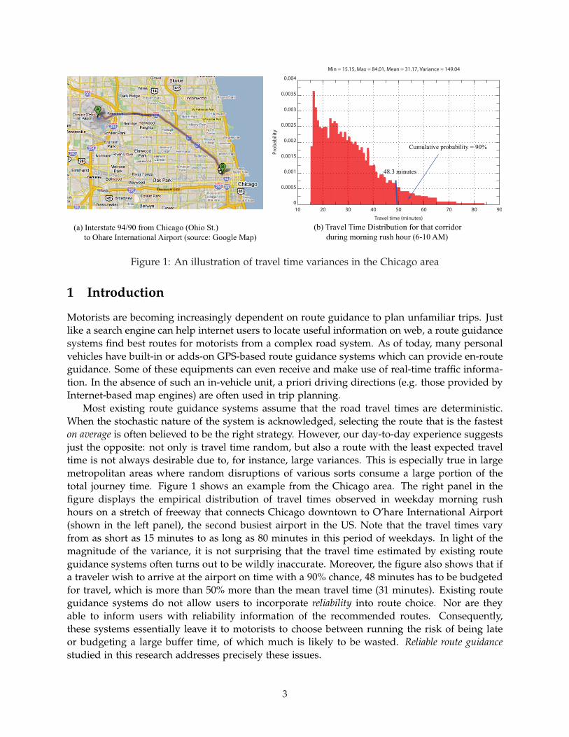
This research uses the GCM data as the primary source for traffic data on freeways and tollroads. The GCM data come from two main sources: loop detectors and electronic toll transpon-ders (I-PASS), which cover freeways and toll roads respectively. Figure 2 shows the Chicagonetwork used in the case study, as well as the location of loop detectors and IPASS toll booths.The network data are from the latest travel planning model prepared by the Chicago Metropoli-tan Agency for Planning (CMAP). As revealed in Figure 2, a major problem is the lack of dataon arterial and local streets, which constitute the majority of links in the network. Recognizingthat this is a universal problem that has not yet been overcome in the current paradigm of datacollection, we estimate travel time distributions on these streets, as to be detailed in Section 4.2.

9

Filled circles: Loop detector

Unfilled circles: Toll plaza

Airport

Chicago

Northshore

South suburbs

Figure 2: The Chicago network from Chicago Metropolitan Agency for Planning

10

4.1 Data for freeway and toll roads

In the GCM database, loop detectors record speed, occupancy and flow rate approximately every5 minutes. Likewise, travel times on toll roads between two I-PASS toll booths are obtainedfrom in-vehicle transponders, and subsequently aggregated and written into database every 5minutes. About 825 loop detectors and 174 I-PASS detectors (each I-PASS detector correspondsto an origin-destination pair of toll booths) from GCM database are used in this study (see Figure2). Specifically, the loop detector data collected from 10/10/2004 to 10/11/2008, and the I-PASSdetector data from 10/9/2004 to 7/3/2008, are employed.

We first need to identify links that are “covered” by either I-PASS detector or loop detector. Todetermine which link in the CMAP network is associated with a loop detector, the coordinates(longitude and latitude) of the detector are used to find the closest freeway link. Finding theI-PASS covered links requires more work, which consists of two major steps. In the first, thestarting and ending points of the I-PASS detector are located in the CMAP network. The secondstep identifies and marks all links used by the fastest (not shortest) path connecting the twopoints. Thus, vehicles that pass two I-PASS toll booths in sequence are assumed to always stayon the toll roads, which in most cases constitute the fastest alternative. Note that a link in theCMAP network may be covered by more than one loop detector. In total, 765 out of 44331 linksare covered in one way or another, as shown in Figure 3.

For links covered by loop detector(s), the recorded speed in a 5-minute interval is used toestimate link travel time for the corresponding interval, i.e.,

τda (t) = la/vd

a(t) (4)

where τda (t) and vd

a(t) are travel time and speed on link a recorded by detector d for time intervalt, and la is the link length. If for an interval, a link contains more than one recorded travel time,the arithmetic average of calculated travel time values is taken as the nominal link travel time,that is,

τda (t) =

∑d∈D(a) la/vda(t)

|D(a)| (5)

where D(a) is the set of loop detectors associated with link a at a given time. As for I-PASSdetectors, we need to estimate link travel times on covered link based on the recorded pathtravel times for a given time period. This is a difficult exercise for two reasons. First, how thetravel delays (if there is any) experienced on a path may be spatially distributed is unknown.Second, an I-PASS record tagged by one time interval might contribute to link travel times atother time intervals 3. It is hard to solve either problem unless further information is available,such as supplementary loop detector data. For simplicity, we assume that path travel times aredistributed to links proportional to their lengths, that is

τia(t) =

la

∑a∈krs lacrs

k (t) (6)

where krs denotes the shortest path connecting nodes r (the starting node of the link associatedwith the origin toll booth) and s (the ending node of the link associated with the destinationtoll booth), and crs

k (t) is the recorded travel time on the path for time interval t. While this

3Note that the time interval that identifers an I-PASS record must be tied to either the entry (origin) or exit(designation), since the travel times between most I-PASS toll booths are longer than 5 minutes.

11

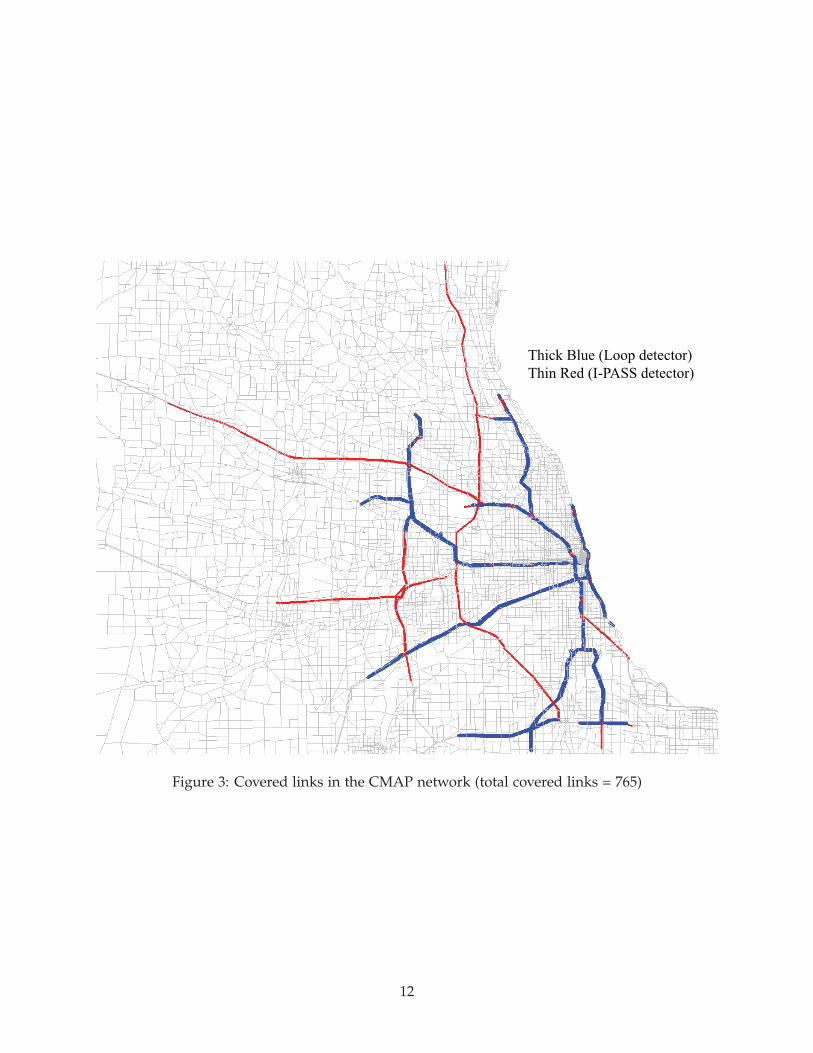
Thick Blue (Loop detector)

Thin Red (I-PASS detector)

Figure 3: Covered links in the CMAP network (total covered links = 765)

12

simplification would certainly introduce errors, we note that the magnitude of errors may bealleviated when multiple I-PASS records are available for the same stretch of toll roads. Equation(6) also implies that the travel time on a path at one time interval contributes to its covered linksfor the same interval. This shortcoming is not as serious as it sounds, since eventually the traveltime data will be aggregated on a period of a coupe of hours. That is to say, as long as themisplaced link travel times do not go into a wrong period (which is certainly possible but ismuch less likely), they will not seriously distort the aggregated distributions. To summarize, thetravel time on link a at time t is given by

τa(t) =

τda (t) if loop data are available

τia(t) if I-PASS data are available

(7)

Once link travel times are obtained, the empirical distributions can be constructed using thefollowing procedure.

Construct Empirical Distribution

Step 1 Find La = minτa(t), ∀t ∈ Λ, Ua = min10la/v0a, maxτa(t), ∀t, where Λ is a set of

valid time intervals, and v0a is free flow speed (or speed limit) on link a.

Step 2 Divide [La, Ua] into M intervals, and let δa = (Ua − La)/M. Find the set Dm = τa(t)|∀t ∈Λ, (m− 1)δa ≤ τa(t) < mδ, ∀m = 1, ...., M

Step 3 Obtain the probability mass for each interval m using Pm = |Dm||Λ| .

It is noted that link travel time distribution may be affected by various factors, such as time-of-day and seasonal effects. Conceivably, one should consider a different reliable routing decisionfor rush hour and off-peak period. To address this issue, the travel time data are disaggregatedaccording to three key factors: time-of-day, day-of-week and season. Specifically, each day isdivided into four periods, namely, morning peak period (6 am - 10 am), mid-of-day period (10am - 3 pm), evening peak period (3 pm - 8 pm) and off-peak period (8 pm - 6 am). Daysin a week are first grouped into weekends and weekdays. In addition, Friday, Saturday andSunday form individual groups because they have somewhat different travel patterns. Finally, ayear is grouped into Spring (months of March, April and May), Summer (months of June, Julyand August), Fall (months of September, October, November) and Winter (months of December,January, February). For each of the three factors, an additional group is added to address thecase of no-segmentation. For instance, the segmentation for time-of-day contains 5 instead of 4groups: morning peak, mid-of-day, evening peak, off-peak and whole-day (no segmentation fortime-of-day). Therefore, in total, there are 5× 6× 5 = 150 possible combinations. Accordingly,we generate 150 different distributions for each of the 765 covered links.

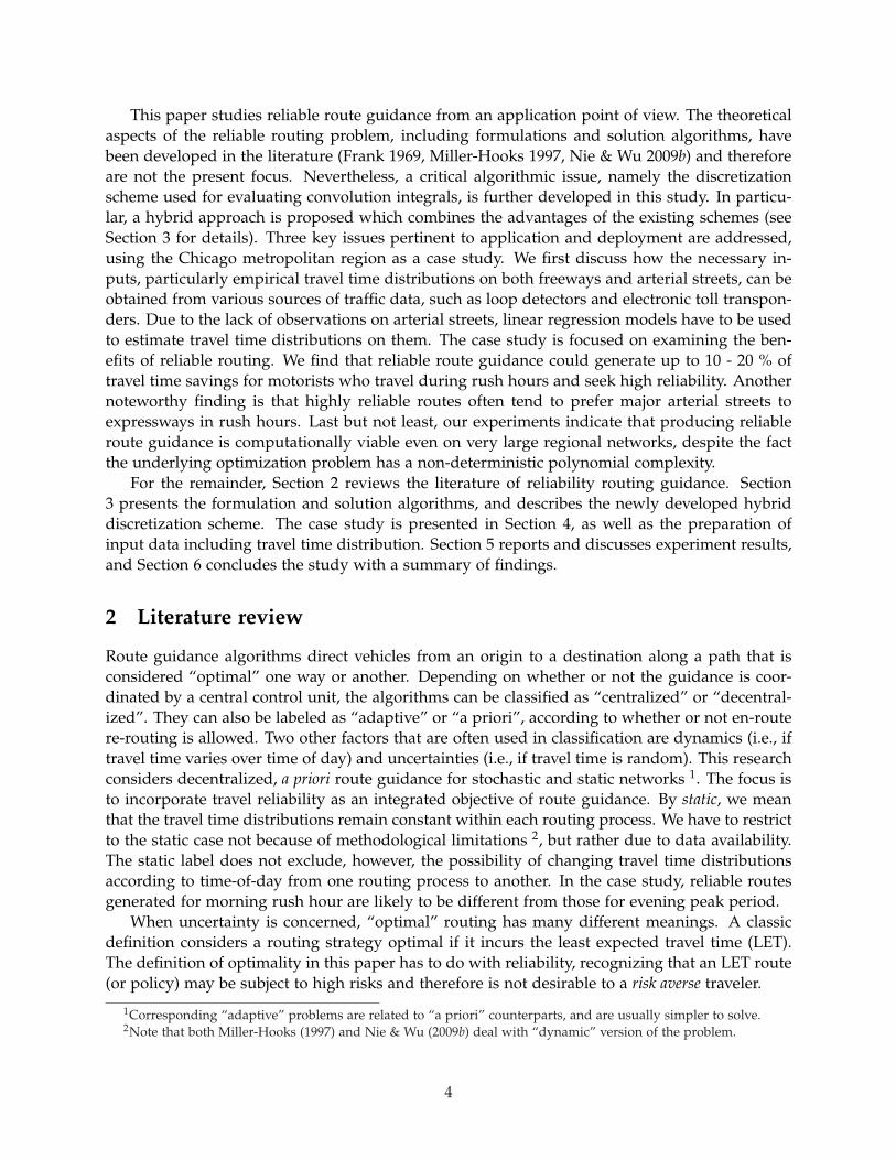
A comparison of travel time distributions on a sample link for the four time-of-day periods isgiven in Figure 4. The results suggest that the most congested period is evening peak, followedby mid-of-day, morning peak and off-peak. Also, the variance of the distributions increases asthe road becomes more congested. For example, the standard deviation for off-peak and eveningpeak is 0.1 and 0.4 minutes, respectively.

4.2 Data for arterial and local streets

No observations are available for arterial and local streets in the CMAP network. Consequently,the travel time distributions on these links have to be estimated indirectly. The estimation process

13

0 0.5 1 1.5 2 2.50

0.005

0.01

0.015

0.02

Travel time (minutes)

Pro

ba

bil

ity

N = 8827, Min = 0.37, Max = 4.23, Mean = 0.66, Var = 0.07

0 0.5 1 1.5 20

0.005

0.01

0.015

0.02

Travel time (minutes)

N = 13406, Min = 0.43, Max = 3.11, Mean = 0.73, Var = 0.10

0 0.5 1 1.5 20

0.005

0.01

0.015

0.02

Travel time (minutes)

Pro

ba

bil

ity

N = 8989, Min = 0.42, Max = 2.94, Mean = 0.88, Var= 0.17

0 0.5 1 1.5 20

0.005

0.01

0.015

0.02

Travel time (minutes)

N = 21350, Min = 0.37, Max = 1.44, Mean = 0.47, Var = 0.01

Morning PeakMid-of-day

Evening Peak Off-peak

Figure 4: Comparison of link travel time distribution at different time-of-day periods (Link 19815,Spring, Weekday)

14

involves two main steps: select an appropriate functional form, and estimate its parameters.Travel time on freeways and arterial streets is known to closely follow a Gamma distribution

(e.g. Polus 1979). Figure 4 provides further confirmation. Gamma distributions have also beenadopted in various studies of stochastic routing problems (e.g. Fan, Kalaba & Moore 2005, Nie& Wu 2009b). Therefore, this study adopts Gamma distribution to describe the travel time dis-tribution on arterial and local streets. The probability density function of a Gamma distributionis

f (x) =1

θκΓ(κ)(x− µ)κ−1e−(x−µ)/θ ; x ≥ µ, θ, κ ≥ 0 (8)

where θ is the scale parameter; κ is the shape parameter; µ is the location parameter; and Γ(·) is theGamma function which takes the following form

Γ(z) =∫ ∞

0tz−1e−tdt

Having selected the functional form, we proceed to show how to estimate the three param-eters required in a Gamma distribution. We first note that the mean and variance of a Gammadistribution are κθ and κθ2, respectively. Thus, if we know mean (denoted as u), variance (de-noted as σ2) and µ, then κ and θ can be obtained by

θ =σ2

u− µ, κ = (

u− µ

σ)2 (9)

The CMAP travel demand model (CMAP 2006) is used to estimate congested travel times onarterial streets. Note that the planning model is designed to capture average traffic conditionsin the network for the designated time period on a typical weekday. The CMAP travel demandmodel represents a classical four-step process of trip generation, trip distribution, mode choice, andtraffic assignment, with considerable modifications used to enhance the distribution and modechoice procedures. The original CMAP model divides a day into eight periods: off-peak (8 PM- 6 AM), pre-morning-peak (6-7 AM), morning-peak (7 - 9 AM), post-morning-peak (9-10 AM),mid-of-day (10 AM - 2 PM), pre-evening-peak (2 - 4 PM), evening-peak (4 - 6 PM), and post-evening-peak (6 - 8 PM). Note that in GCM data peak periods combine the pre and post periodsdefined in the CMAP model. For simplification, the assignment results for the peak periods(morning and evening) in the CMAP model are used to represent those from pre to post peakperiods. Specifically, each link obtains from the CMAP model a mean travel time for each of thefour predetermined GCM periods: morning peak, mid-of-day, evening peak and off-peak.

We postulate that the mean and variance of travel times on a link are related to its freeflow travel time τ0 and the level of congestion ρ = τ − τ0, where τ is travel time from trafficassignment (note that the subscript a is suppressed for simplicity). This relationship may beestimated from freeway data using statistical models. The simplest linear regression model reads

u = a1τ0 + b1ρ + c1 (10)

σ = a2τ0 + b2ζρ + c2 (11)

where a1, b1, c1, a2, b2 and c2 are coefficients to be estimated from linear regression. ζ is a pre-determined parameter to account for the fact that the existence of signal control may increasevariances. ζ = 1 if no signal exists on the link; otherwise ζ is taken from a uniform distribution

15

Table 2: Results of the linear regression for the mean-variance model (Equations 10-11) and thelocation model (Equation 12)

time-of-day Variance Model Mean Model Location Modelperiods a1 b1 c1 R2 a2 b2 c2 R2 a b R2

AM PEAK 0.309 0.870 0.580 0.444 1.127 0.546 -2.056 0.910 0.843 -4.106 0.958PM PEAK 0.368 0.685 2.967 0.400 1.143 0.563 0.336 0.872 0.860 -3.533 0.964MIDDAY 0.283 1.076 2.040 0.346 1.100 0.630 -1.145 0.889 0.857 -3.608 0.956

OFF PEAK 0.178 0 -1.031 0.516 1.043 0 -5.854 0.907 0.831 -5.257 0.937

between [1.1, 1.3]. For all 765 links covered by GCM data, u and σ can be obtained from theempirical distribution and ρ is known from the CMAP travel demand model. Thus, a linear re-gression can be performed to determine the coefficients, which in turn are employed to estimateu and σ for arterial streets. We note that a linear model is needed for each of the four time-of-dayperiods.

A similar linear model can be constructed to estimate the location parameter µ, which delin-eates the smallest possible travel time on a link. We note that µ is likely to be smaller than τ0

because motorists may drive well beyond the speed limit or the nominal ”free-flow travel speed”.Moreover, it seems reasonable to assume that the level of congestion does not affect µ. Thus, thelinear model used to estimate µ is given by

µ = aτ0 + b (12)

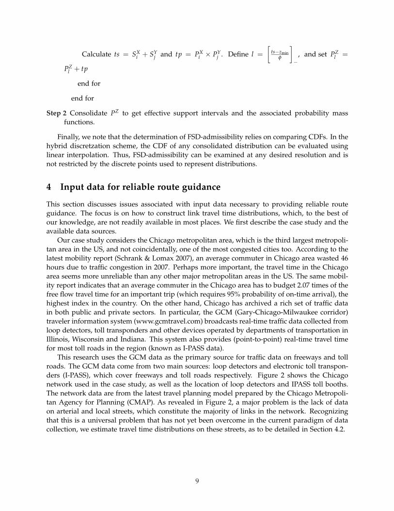
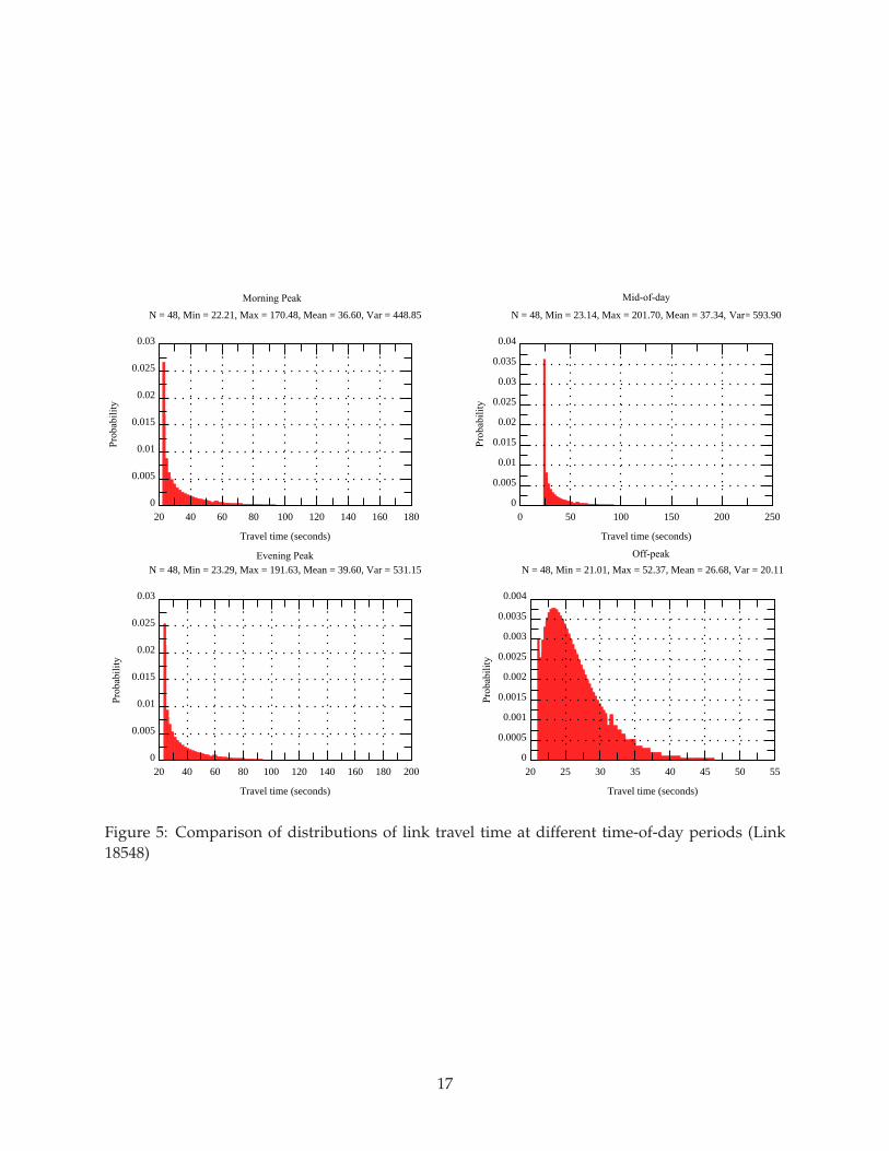
The linear regression results for each of the four time-of-day periods are given in Table 2.As shown, the mean model and the location model (Equation 12) fit the data rather well (highR2). However, the fitness of the variance model is not impressive. We tried, without muchsuccess, to introduce various forms of non-linearity into the model, such as using the variance(σ2) instead of the standard deviation on the left hand side of Equation (11), or consider ρ2 onthe right hand side. Apparently, the travel time variances are affected by many other factors notincluded in the simple linear model. A more in-depth investigation of the variance model is leftto the future research. Finally, we note that the coefficient of the congestion index is near zero inboth mean and variance models for the off-peak period because congestion is negligible in thatperiod. Figure 5 reports distributions on a sample link (located on the northbound Columbus Dr.in the Chicago downtown). The results show that the street is slightly more congested duringthe mid-of-day and evening peak periods.

5 Experimental results and discussions

Numerical experiments are presented in this section to show the usefulness of reliable routeguidance and the feasibility of the existing algorithm in solving the real-size problems. For thefirst, we consider two real-world routing examples: one is between Chicago downtown and theO’hare international airport (ORD); another is from the northshore to Chicago south suburbs.Only the three non-off-peak periods in weekdays are considered. The algorithm FSD-LC was

16

20 40 60 80 100 120 140 160 1800

0.005

0.01

0.015

0.02

0.025

0.03

Travel time (seconds)

N = 48, Min = 22.21, Max = 170.48, Mean = 36.60, Var = 448.85

0 50 100 150 200 2500

0.005

0.01

0.015

0.02

0.025

0.03

0.035

0.04

Travel time (seconds)

Prob

abili

ty

N = 48, Min = 23.14, Max = 201.70, Mean = 37.34, SD = 593.90

20 40 60 80 100 120 140 160 180 2000

0.005

0.01

0.015

0.02

0.025

0.03

Travel time (seconds)

N = 48, Min = 23.29, Max = 191.63, Mean = 39.60, Var = 531.15

20 25 30 35 40 45 50 550

0.0005

0.001

0.0015

0.002

0.0025

0.003

0.0035

0.004

Travel time (seconds)

Prob

abili

ty

N = 48, Min = 21.01, Max = 52.37, Mean = 26.68, Var = 20.11

Var

Probability

Probability

Probability

Probability

Morning Peak Mid-of-day

Evening Peak Off-peak

Figure 5: Comparison of distributions of link travel time at different time-of-day periods (Link18548)

17

(a) Typical path from downtown to ORD (b) Typical path from ORD to downtown

Figure 6: FSD-admissible paths between Chicago downtown and ORD during the mid-of-dayperiod of weekdays

coded using MS-C++ and tested on a Windows XP x64 Workstation with two Xenon 3.0GHzCPUs and 8GB RAM.

5.1 From Chicago downtown to O’hare international airport (ORD)

In this experiment, the intersection of Wabash St. and Washington St. is selected to represent theChicago downtown, and the airport is represented by the end of I-190, the highway that servesthe terminals. The most obvious choice for this routing problem, which is also suggested by bothGoogle Map and Yahoo Maps, is to use freeway I-90/94 and I-90. Our results agree with thispopular routing policy in general but have interesting discrepancies. For the mid-of-day period,most FSD-admissible paths do heavily use I-90 and I-90/94, and the differences between thesepaths are trivial, see Figure 6.

For the morning peak period, however, the reliable route guidance suggests that motoristsshould avoid I-90/94 and use an arterial street (N. Milwaukee Ave.) instead, if they wish to havean on-time arrival probability higher than 44% (to airport) or 62% (from airport) on-time arrivalprobability. To arrive at the airport with 95% probability, for example, the path in Figure 7(a)requires a time budget of 33 minuets 57 seconds while the path mostly using I-90 and I-90/94needs 37 minutes and 18 seconds. The reliable route guidance thus leads to a 10% saving intravel budget. In the evening peak of weekdays, motorists who drive from the airport to the cityare recommended to avoid I-90 until they pass the diverge of I-90 and I-94 (see Figure 8(a)). For95% on-time arrival probability, the path in Figure 8(a) requires a time budget of 34 minutes and30 seconds, while the path in Figure 8(b) needs 39 minutes and 38 seconds. In both periods,our results suggest that avoiding the entire or part of the popular freeways will help motoristsbudget less time for better reliability.

We note that the path given in Figure 8(b) is actually the best for 50% on-time arrival proba-bility (i.e. the average performance). At this probability, a motorisit using the path only need tobudget 34 minutes 17 seconds for travel. As a comparison, the more reliable path in Figure 8(a)needs a slightly higher budget (34 minutes 34 seconds) for 50% probability.

Figure 9 reports the CDFs of travel times on the FSD-admissible paths. Note that the CDFsduring the mid-of-day period are very close to each other. A close look reveals that all theseadmissible paths heavily use I-90/94 and I-90, with negligible topological differences. On theother hands, the CDFs for the morning and evening peak periods are quite different, which are

18

(a) from downtown to ORD (b) from ORD to downtown

Figure 7: Shortest paths between Chicago downtown and ORD ) during the morning peak ofweekdays (desired on-time arrival probability = 95%)

(a) 95% on-time arrival probability (b) 50% on-time arrival probability

Figure 8: Shortest paths from ORD to Chicago downtown during the evening peak of weekdays

19

24 26 28 30 32 34 36 38 40 420

0.2

0.4

0.6

0.8

1

Time (minutes)

Cumulativeprobability

Morning Peak of Weekdays

(a)

20 22 24 26 28 30 320

0.2

0.4

0.6

0.8

1

Time (minutes)

Cum

ulat

ive

prob

abili

ty

Mid-of-day Peak of Weekdays

Cumulativeprobability

(b)

22 24 26 28 30 32 34 36 380

0.2

0.4

0.6

0.8

1

Time (minutes)

Evening Peak of Weekdays

Cumulativeprobability

(c)

Figure 9: Cumulative density functions (CDFs) of travel times on FSD-admissible paths for tripsfrom Chicago downtown to ORD during different time periods

related to the substantial topological difference of the admissible paths.

5.2 From the northshore to south suburbs

The challenge of this routing problem (see Figure 2) is how to travel through the Chicago down-town and its congested peripheral area. Typically, motorists have two options: I-90/94 and LakeShore Dr. The origin and the destination are deliberately selected so that both options couldbecome attractive. Specifically, the intersection of Illinois Rd. and Locust Rd. on the northshore,and the intersection of E.79 St. and S Martin Luther King Dr. in the south suburbs are selected.The reliable route guidance generally suggests that for weekdays motorists should stay awayfrom I-90/94, especially for the portion north of Chicago downtown if driving from north tosouth. Our results indicate that the popular choice shown in Figure 10(a) is shortest only whenthe on-time arrival probability is very low (6% for morning peak, and 18% for mid-of-day). Forthe evening peak, this path is not even FSD-admissible. For the mid-of-day and the eveningpeak periods, Lake Shore Dr. is more reliable. Figure 10(d) shows that the shortest path duringthe mid-of-day period uses the Lake Shore Dr, which guarantees an on-time arrival probabilityhigher than 43%. The FSD-admissible paths for the evening peak are similar and not reportedseparately. For the morning peak, however, Lake Shore Dr. is preferred only if a motorist wantsto arrive on time with a probability lower than or equal to 59% (see Figure 10(c)). For higherreliability motorists need to use various arterial streets until they are close to downtown, andthen switch I-90/94 (see Figures 10(b)).

Driving from south to north during weekdays is a different story. Experiments show thatthe path in Figure 10(a) (reverse direction) represents most of FSD-admissible path with theexception of the morning peak. For that period, Lake Shore Dr. is always recommended and anypath using I-90/94 is not FSD-admissible.

20

(a) (b) (c) (d) (e)

Figure 10: Shortest paths from northshore to south suburbs or in the reverse direction

5.3 Computational performance

Table 3 reports the consumed CPU times for solving each of the two routing problems in eitherdirection and in both weekends and weekdays 4. As shown, the RASP problem was solvedwithin 30 seconds in most cases. Considering the complexity of the problem and the sheer sizeof the network, the performance is acceptable even from a practical point of view. Note that ouralgorithm actually finds FSD-admissible paths from all origins to the destination simultaneously.Therefore, once the computation is done for one O-D pair, little further efforts are needed toobtain admissible paths from another origin to the same destination. It may be possible toexpedite the computation if the route guidance is only needed for one O-D pair. This possibility,however, is not explored in the current implementation.

Table 3 reveals that solving the weekend models generally took shorter CPU times and gen-erated fewer admissible paths. We conjecture that this is because the roads are less congested onweekends, and therefore subject to smaller travel time variances. Particularly, the morning andevening periods on weekends often have only one admissible path; the most obvious choice (i.e.major freeways) usually prevails in those cases.

In order to better understand the impacts of travel time variances, a sensitivity analysis isconducted in the following. The focus is given to the variances on arterial streets, since the linearregression model used to estimate them was not fitted very well. In the analysis, we simplymultiply the estimated variances on arterial by a parameter λ = 0.5, 1.0, 1.5, 2.0, 2.5, and 3.0. Foreach value of λ (called a scenario), five different locations in the CMAP network are selected tocompute the all-to-one reliable shortest paths. Three performance indexes are recorded for eachrun: the CPU time, the average and maximum number of FSD-admissible paths at all nodes.The average of the five runs (each for one destination) are used as the performance index forthe scenario. Figure 11 shows how these indexes vary with the value of λ. Clearly, as the

4In fact, the same travel time distributions are used on arterial streets for both weekends and weekdays. Coveredlinks, however, have different distributions on weekends and weekdays from observations.

21

Table 3: Computation performance of the algorithm in the two routing problems

Weekdays WeekendsAM Peak Mid-of-day PM Peak AM Peak Mid-of-day PM Peak

Downtown to ORDCPU time 29.58 18.69 16.58 12.25 19.14 8.50

# paths 7 5 4 1 5 1ORD to downtownCPU time 29.58 23.70 14.58 15.69 15.36 28.02

# paths 6 2 2 1 2 4Northshore to south suburbsCPU time 65.88 74.39 20.42 15.52 46.53 33.74

# paths 7 10 2 2 1 4South suburbs to northshoreCPU time 60.83 39.00 33.74 14.19 36.25 12.08

# paths 10 6 6 1 3 1

Note: 1) CPU time is measured in seconds; 2) ”# paths” stands for the number of FSD-admissible paths

variances increase, the average size of FSD-admissible paths grows. As a consequence, it takesthe algorithm longer to solve the problem; note that the complexity of the algorithm depends onthe size of FSD-admissible paths (Nie & Wu 2009b). The good news is that the CPU time doesnot seem to increase superlinearly with the variances. In fact, the CPU time barely doubled whenthe variances on arterial streets become six time higher. The longest average CPU times is stillless than one minute, which remains acceptable for practical purposes.

0.5 1 1.5 2 2.5 325

30

35

40

45

50

55

60

CP

U t

ime

(s

ec

on

d)

0.5 1 1.5 2 2.5 30

2

4

6

8

10

0.5 1 1.5 2 2.5 30

50

100

150

200

λ λ λ

Figure 11: Impacts of travel time variances (arterial streets) on computational performance

22

6 Summary

The overarching goal of this research is to demonstrate that incorporating reliability measuresinto routing decisions is both useful and feasible. To these ends, we present a proof-of-conceptcase study of reliable route guidance on a large regional network from the Chicago area.

Our experiments indicate that best paths do vary substantially with the reliability require-ment, measured in this paper by the probability of arriving on-time or earlier. For motorists whotravel during rush hours and seek high reliability, reliable route guidance could generate up to10 - 20 % of travel time savings. Interestingly, highly reliable routes often tend to prefer majorarterial to freeways and highways in rush hours. This phenomenon could well have been causedby the underestimation of travel time variances on arterial streets, recalling that the distributionson arterial streets were estimated using linear models calibrated from freeway data, which werenot fitted very well for the variances. Nevertheless, staying away from congested freeways dur-ing rush hours, particularly when you have important appointments, does seem to agree withconventional wisdom. Such advice appeals to many motorists probably because freeways areless amenable to effective recourses when uncertainty strikes. The results from this case studymay have provided a piece of empirical evidence to support this perception.

The paper presents and implements methods for constructing link travel time distributions,which are key inputs to providing reliable route guidance. Since these methods primarily rely ontraffic and travel planning data that are available in many (if not most) large metropolitan areasin the US, they can be transferred to other regions upon further validation. A major problemtackled in this research is the data availability on arterial and local streets. Hitherto little trafficinformation has been archived for these streets, even on those equipped with intersection-relatedsensors. The method proposed in this research is indeed a compromise instead of a resolution.On the one hand, that the level of congestion affects travel time variances is widely noticed, andindeed supported by our data. Therefore, predicting variances from a congestion index seemsa reasonable idea. On the other hand, it is likely that travel time variances depend on manyother factors in a complex manner, and therefore the simple linear model may not work verywell. After all, using freeway data to estimate distributions on arterial streets may turn out tobe inappropriate, since these links have quite different characteristics. It will be more desirableto calibrate the models using travel time data directly collected on arterial streets. Currently, theresearch team is seeking to use AVL (automatic vehicle location) data collected by buses. We willreport those results in a subsequent work.

The study also verifies the capability of existing algorithms in solving large-scale reliablerouting problems within reasonable amount of time. As noted, in most cases the algorithm foundall-to-one reliable paths (FSD-admissible paths) within a minute on an up-to-date workstation.Considering the non-deterministic polynomial complexity of the problem and the sheer sizeof the network, the reported performance is deemed satisfactory. To perform reliable routeguidance in real-time (e.g., through an en-vehicle navigation system), further improvements arestill needed. Possible strategies include but are not limited to: imposing higher-order stochasticdominance to reduce the number of non-dominant paths; adopting approximation methods; andexploiting the special properties of a one-to-one (instead of all-to-one) shortest path problem. Weleave these further developments also to the future research.

Finally, it is worth noting that the methodologies presented herein can be used in applicationsother than reliable route guidance. They can help, for instance, transportation planning agencyunderstand the level of service in terms of reliability in heavily traveled corridors, or construct

23

aggregated travel reliability indexes for the entire or part of the highway network of interest.

Acknowledgements

The authors want to thank Mr. Kermit Wies from the Chicago Metropolitan Agency for Plan-ning, for providing the CMAP network and travel demand data used in this project. This re-search is funded by the Center for the Commercialization of Innovative Transportation Technol-ogy (CCITT) at Northwestern University.

References

Carraway, R. L., Morin, T. L. & Moskowitz, H. (1990), ‘Generalized dynamic programming formulticriteria optimization’, European Journal of Operational Research 44(1), 95–104.

Chen, Y., Bell, M. G. H., Wang, D. & Bogenberger, K. (2006), ‘Risk-averse time-dependent routeguidance by constrained dynamic a* search in decentralized system architecture’, Transporta-tion Research Record 1944, 51–57.

CMAP (2006), Travel demand modeling for the conformity process in northeastern illinois,available at http://www.cmap.illinois.gov /uploadedfiles/publications/other publications/pm25 conformity analysis b.pdf, last accessed on 6/10/2009, Chicago MetropolitanAgency for Planning.

Eiger, A., Mirchandani, P. B. & Soroush, H. (1985), ‘Path preferences and optimal paths in prob-abilistic networks’, Transportation Science 19(1), 75–84.

Fan, Y., Kalaba, R. & Moore, J. (2005), ‘Arriving on time’, Journal of Optimization Theory andApplications 127(3), 497–513.

Frank, H. (1969), ‘Shortest paths in probabilistic graphs’, Operations Research 17(4), 583–599.

Hadar, J. & Russell, W. (1969), ‘Rules for ordering uncertain prospects’, American Economic Review59, 25–34.

Kaparias, I., Bell, M., Chen, Y. & Bogenberger, K. (2007), ‘Icnavs: a tool for reliable dynamic routeguidance’, IET Intellegent Transportation Systems 1(4), 225–253.

Loui, R. P. (1983), ‘Optimal paths in graphs with stochastic or multidimensional weights’, Com-munications of the ACM 26(9), 670–676.

Miller-Hooks, E. (1997), Optimal Routing in Time-Varying, Stochastic Networks: Algorithmsand Implementations, PhD thesis, Department of Civil Engineering, University of Texas atAustin.

Miller-Hooks, E. D. & Mahmassani, H. S. (1998a), ‘Least possible time paths in stochastic, time-varying networks’, Computers and Operations Research 25(2), 1107–1125.

Miller-Hooks, E. D. & Mahmassani, H. S. (2003), ‘Path comparisons for a priori and time-adaptive decisions in stochastic, time-varying networks’, European Journal of Operational Re-search 146(2), 67–82.

24

Miller-Hooks, E. & Mahmassani, H. (1998b), On the generation of nondominated paths in stochas-tic, time-varying networks, in ‘Proceedings of TRISTAN III (Triennial Symposium on Trans-portation Analysis)’, San Juan.

Miller-Hooks, E. & Mahmassani, H. (1998c), ‘Optimal routing of hazardous materials in stochas-tic, time-varying transportation networks’, Transportation Research Record 1645, 143–151.

Mirchandani, P. B. (1976), ‘Shortest distance and reliability of probabilistic networks’, Computersand Operations Research 3(4), 347–355.

Montemanni, R. & Gambardella, L. (2004), ‘An exact algorithm for the robust shortest pathproblem with interval data’, Computers and Operations Research 31(10), 1667–1680.

Murthy, I. & Sarkar, S. (1996), ‘A relaxation-based pruning technique for a class of stochasticshortest path problems’, Transportation Science 30(3), 220–236.

Murthy, I. & Sarkar, S. (1998), ‘Stochastic shortest path problems with piecewise linear concavelinear functions’, Management Science 44(11), 125–136.

Nie, Y. & Wu, X. (2009a), ‘Reliable a priori shortest path problem with limited spatial and tem-poral dependencies’, In Proceedings of the 18th International Symposium on Transportation andTraffic Theory, accepted .

Nie, Y. & Wu, X. (2009b), ‘Shortest path problem considering on-time arrival probability’, Trans-portation Research Part B 43, 597–613.

Polus, A. (1979), ‘A study of travel time and reliability on arterial routes’, Transportation 8(2), 141–151.

Schrank, D. & Lomax, T. (2007), 2007 urban mobility study, Technical report, Texas TransportationInstitute, Texas A&M University, College Station, TX.

Sen, S., Pillai, R., Joshi, S. & Rathi, A. (2001), ‘A mean-variance model for route guidance inadvanced traveler information systems’, Transportation Science 35(1), 37–49.

Sigal, C. E., Alan, A., Pritsker, B. & Solberg, J. J. (1980), ‘The stochastic shortest route problem’,Operations Research 28(5), 1122–1129.

Sivakumar, R. & Batta, R. (1994), ‘The variance-constrained shortest path problem’, TransportationScience 28(4), 309–316.

von Neumann, J. & Morgenstern, O. (1967), Theory of Games and Economic Behavior, Wiley, NewYork.

Wu, X. & Nie, Y. (2009), ‘Implementation issues in approximate algorithms for reliable a priorishortest path problem’, Journal of the Transportation Research Board Forthcoming.

Yu, G. & Yang, J. (1998), ‘On the robust shortest path problem’, Computers and Operations Research25(6), 457–468.

25