Embed Size (px)
Citation preview

1
psyc3010 lecture 4
interpretation of anova
higher order designs (complex anova)
Before Ekka: following up effects & magnitude of effects in 2-way
next week: power analysis

2
last week this week
Before the break, we looked at how to follow-up
significant main effects and interactions, and
how to calculate effect size
this week we briefly consider interpretation of
factorial anova, before moving on to higher order
factorial designs (sometimes called „complex
anova‟)
We also distribute Assignment 1 (which can also
be downloaded from the course website)

3
topics for this week
interpreting 2-way factorial ANOVA review of omnibus tests + follow-up effects
notes on reporting effects
introduction to higher-order designs
omnibus tests in 3-way factorial ANOVA main effects
2-way interactions
3-way interactions
following up 3-way factorial ANOVA simple interaction effects
simple simple effects
simple simple comparisons

4
wrapping up the distraction study:
hypotheses we might have had for our study…
1) we predict that creativity will be higher when more alcohol
is consumed
(hence, we predict a main effect of consumption)
2) we predict that creativity will be lower when distracted
(hence, we predict a main effect of distraction)
3) we predict that the effect of consumption on creativity
ratings will be stronger for distracted participants
(hence, we predict an interaction
between distraction and consumption)

5
Summary Table – from lectures 2 and 3
Source df SS MS F sig
C (cons) 2 3332.3 1666.15 20.07 .000
D (dist) 1 168.75 168.75 2.03 .161
C x D 2 1978.12 989.06 11.91 .000
Error 42 3487.5 83.02
Total 47 8966.7
interpretationa main effect of
consumption
i.e., there is a significant difference among the marginal
means for consumption …
consumption has
> 2 levels (0, 2 or
4 pints) so we
need to conduct
follow-up tests
to interpret

6
0 pints 2 pints 4 pints
63.75 64.69 46.56
Contrast 1 2 -1 -1
Contrast 2 0 1 -1
Consumption
these are the marginal
means for consumption
from our data table earlier
a set of weights (aj) is used to
define the contrasts:
contrast 1 compares 0 vs 2 & 4
contrast 2 compares 2 vs 4
abNdferror dn
MSa
Lt
errorj
*
2
jj XaL
t’=.05 (42) = 2.33 (Bonferroni adj)
results of linear contrasts:
comparison 1: t’(42) = 2.91, p<.05
comparison 2: t’(42) = 5.63, p<.05
“Here’s a set of Linear
Contrasts I prepared earlier…”

7
Summary Table – from lectures 2 and 3
Source df SS MS F sig
C (cons) 2 3332.3 1666.15 20.07 .000
D (distr) 1 168.75 168.75 2.03 .161
C x D 2 1978.12 989.06 11.91 .000
Error 42 3487.5 83.02
Total 47 8966.7
interpretationa main effect of
distraction
i.e., there is no significant difference among the marginal
means for distraction
main effect is not
significant so no
further analysis is
needed
8
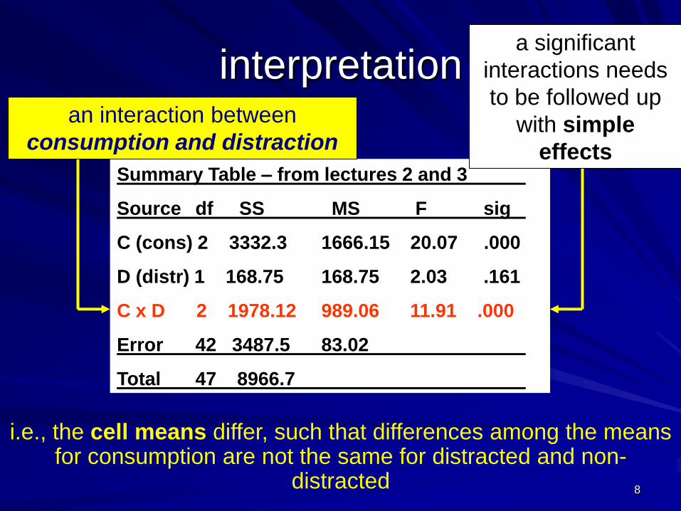
Summary Table – from lectures 2 and 3
Source df SS MS F sig
C (cons) 2 3332.3 1666.15 20.07 .000
D (distr) 1 168.75 168.75 2.03 .161
C x D 2 1978.12 989.06 11.91 .000
Error 42 3487.5 83.02
Total 47 8966.7
interpretationan interaction between
consumption and distraction
i.e., the cell means differ, such that differences among the means for consumption are not the same for distracted and non-
distracted
a significant
interactions needs
to be followed up
with simple
effects

9
a note on interactions…
some sources suggest that once you find a significant interaction you should ignore the main effects as the main effects have been “qualified” by the interaction
this is because the interaction may require you to change the interpretation given by the main effect alone (but then again, it may not – see Howell section 13.3)
ultimately, there is no simple rule: what you report depends entirely upon your research predictions – if you predict a main effect, then report that main effect (and any follow-up tests)
– in our case, we made a specific prediction about both of our main effects, so we should deal with them accordingly

10
reporting“Results indicated a significant main effect of consumption, F(2,42) = 20.07,
p<.001, ω2 = .34. Linear contrasts with a Bonferroni adjustment for 2 comparisons
indicated that creativity ratings were significantly lower after 2 or 4 pints than after
consuming no alcohol, t’(42) = 2.91, p<.05 (Ms = 63.75, 55.63), and were lower
after 4 pints than after 2 pints, t’(42) = 5.63, p<.05 (Ms = 64.69, 46.56). There was
no significant main effect for distraction, indicating that creativity ratings for
distracted participants‟ limericks (M = 56.46) were not significantly different from
those for controls (M = 60.21), F(1,42) = 2.03, p = .16, ω2 = .01. There was,
however, a significant interaction between consumption and distraction, indicating
that the effect of consumption was different for distracted and control participants,
F(1,42) =11.91, p<.001, ω2 = .20.”
NB Interaction needs following up in results section (simple effects + simple
comparisons if nec.).
Discuss: although the predicted main effect of alcohol consumption was significant,
the direction of the effect was contrary to hypotheses: alcohol lowered creativity
ratings. Also the predicted effect of distraction was not significant.
I haven‟t put effect sizes in for the
follow-up comparisons / contrasts;
most do nowadays esp. if report Fs.

11
Following up the significant
interaction - Simple Effects from
last week:
Source SS df MS F p
C at D1 5208.33 2 2604.17 31.36 0.000
C at D2 102.08 2 51.04 0.61 0.546
D at C1 156.25 1 156.25 1.88 0.177
D at C2 76.56 1 76.56 0.92 0.342
D at C3 1914.06 1 1914.06 23.05 0.000
Error 3487.5 42 83.04
F at alpha=.05 (2,42) = 3.23 if obtained F exceeds critical F reject the null hypothesis
F at alpha=.05 (1,42) = 4.08
2 simple effects
are significant
There is a significant effect of distraction at the third level of
consumption: the mean creativity ratings for distracted and
control participants who have consumed 4 pints are
significantly different (no follow up needed as only 2 levels)

12
Following up the significant
interaction - Simple Effects from
last week:
Source SS df MS F p
C at D1 5208.33 2 2604.17 31.36 0.000
C at D2 102.08 2 51.04 0.61 0.546
D at C1 156.25 1 156.25 1.88 0.177
D at C2 76.56 1 76.56 0.92 0.342
D at C3 1914.06 1 1914.06 23.05 0.000
Error 3487.5 42 83.04
F at alpha=.05 (2,42) = 3.23 if obtained F exceeds critical F reject the null hypothesis
F at alpha=.05 (1,42) = 4.08
There is a significant effect of consumption at the first level of
distraction: the mean creativity ratings for distracted differ
depending upon whether they have had 0, 2 or 4 pints
(follow-up tests needed to identify where the difference is)
2 simple effects
are significant
13
0
10
20
30
40
50
60
70
80
0 2 4
Alcohol consumed (pints)
Cre
ati
vit
y
Distraction
Controls
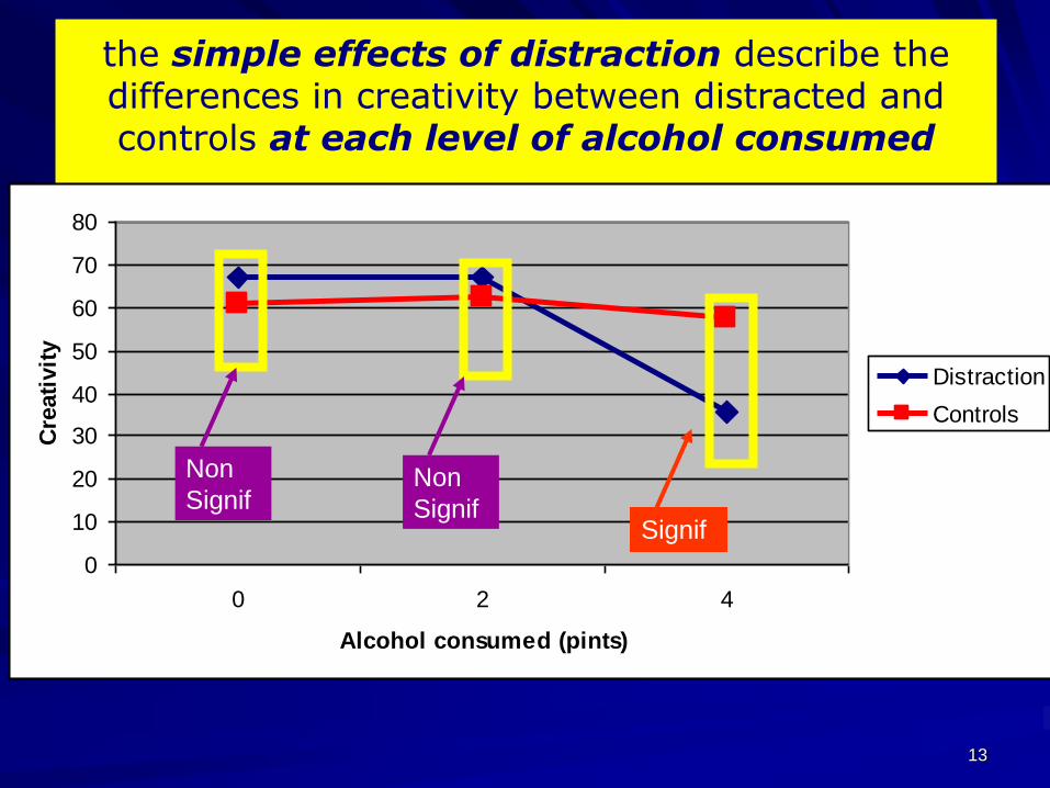
the simple effects of distraction describe the differences in creativity between distracted and controls at each level of alcohol consumed
Non
SignifSignif
Non
Signif

14
Following up the significant
interaction - Simple Effects from
last week:
Source SS df MS F p
C at D1 5208.33 2 2604.17 31.36 0.000
C at D2 102.08 2 51.04 0.61 0.546
D at C1 156.25 1 156.25 1.88 0.177
D at C2 76.56 1 76.56 0.92 0.342
D at C3 1914.06 1 1914.06 23.05 0.000
Error 3487.5 42 83.04
F at alpha=.05 (2,42) = 3.23 if obtained F exceeds critical F reject the null hypothesis
F at alpha=.05 (1,42) = 4.08
There is a significant effect of consumption at the first level of
distraction: the mean creativity ratings for distracted differ
depending upon whether they have had 0, 2 or 4 pints
2 simple effects
are significant

15
0
10
20
30
40
50
60
70
80
0 2 4
Alcohol consumed (pints)
Cre
ati
vit
y
Distracted
Controls
the simple effects of alcohol consumeddescribe the differences in creativity after 0, 2 or 4
pints consumed at each level of distraction
(follow-up tests needed to identify where the difference is)

16
Following up the significant
Simple Effects of consumption
for distracted – simple
comparisons from last week:
abNdferror n
MSa
Lt
errorj
2
jj XaL
t=.05 (42) = 2.33 (Bonferroni adj)
results of linear contrasts:
comparison 1: t(42) = 3.96, p<.05
comparison 2: t(42) = 6.86, p<.05
0 pints 2 pints 4 pints
Distracted 66.88 66.88 35.63
Contrast 1 2 -1 -1
Contrast 2 0 1 -1
Consumption

17
a note on simple effects…
it is preferable to not report all sets of simple effects, for 2 reasons:
a) the more simple effects we calculate, the greater our risk of making a type 1 error (see Howell, p.436)
b) usually both sets of simple effects will communicate similarinformation - redundancy
– so, in our case we would want to report either the simple effects of distraction (at each level of consumption) or the simple effects of consumption (at each level of distraction)
ultimately, there is no simple rule: what you report depends entirely upon your research predictions.
– in our case, we specifically predicted that “the effect of consumption on creativity ratings will be stronger for distracted participants than for controls”. Therefore, we would want to report the simple effects for consumption (and associated simple comparisons / contrasts)

18
reporting
“. . .To follow up the significant two-way interaction, the simple
effects of consumption were analysed at each level of distraction.
There was a significant simple effect of consumption for distracted
participants, F(2,42) = 31.36, p<.001, ω2 = .56, but not for controls,
F(2,42) = 0.61, p = .546, ω2 = .00. The significant effect of
consumption for distracted participants was followed up with Linear
contrasts using a Bonferroni adjustment for 2 comparisons. These
indicated that, for distracted participants, creativity ratings were
lower after 2 or 4 pints than after consuming no alcohol, t’(42) =
4.52, p<.001 (Ms = 66.88, 51.26), and also lower after 4 pints than
after 2 pints, t’(42) = 6.86, p<.001 (Ms = 66.88, 35.63).”
I haven‟t put effect sizes in for the follow-up
comparisons / contrasts ; most do now…. Effect
sizes for simple effects are also required. NB if you
calc w2 for controls it works out to -.01 – a
meaningless % (% cannot be negative), so set to
zero. Another reason some prefer to report eta2.
Discuss: the hypothesis was confirmed that the effect of consumption on
creativity will be stronger for distracted participants than for controls.

19

20
higher-order factorial designs
inclusion of more than 2 independent variables (factors)– Three, four, five …. The world is complex
Consideration of more interactions– In Gender (Male/Female) x Age (Young/Old) x
Nationality (Australian / American) design • Does gender interact with age? Does gender interact with
ethnicity? Does age interact with ethnicity?
• Three two-way interactions considered!
– And the exciting possibility that there is a three-way interaction between age, gender and nationality!

21
Higher order designs
E.g., 2 (age) x 3 (alcohol) x 2 (sex)
between subjects design = 12 cells
Men
No alc 1 drink 5 drinks
Women
No alc 1 drink 5 drinks
Old
Young

22
Higher order designs
main effects for each IV:– differences between marginal means of the factor (averaging
over other factors)
two-way interactions:– examines whether the effect of one factor is the same at every
level of another factor (averaging over the third factor)
three-way interaction:– examines whether the two-way interaction between two factors
is the same at every level of the third factor
– Or: is there variability in the cell means which is not accounted for by the main effects of the IVs and the 2-way interactions?
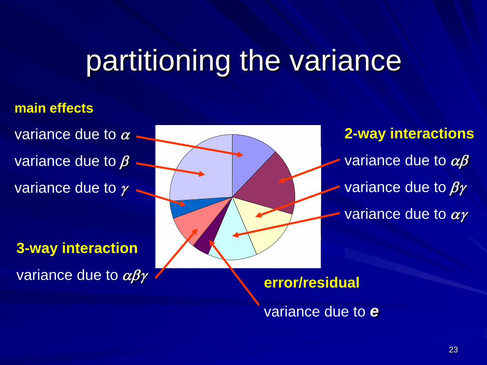
23
partitioning the variance
error
main effects
variance due to
variance due to
variance due to
2-way interactions
variance due to
variance due to
variance due to
3-way interaction
variance due to error/residual
variance due to e

24
higher-order factorial designs
inclusion of more than 2 independent variables (factors)
linear model for a 2-way factorial design:
Xijk = + j + k + jk + eijk
linear model for a 3-way design
Xijkl = + j + k + l + jk + kl + jl + jkl + eijkl

25
3-way data table
Age (2) x alcohol (3) x sex (2)
Men
No alc 1 drink 5 drinks
Women
No alc 1 drink 5 drinks
Old
Young

26
Females
0
200
400
600
800
1000
No drink 1 drink 5 drinks
Alcohol consumption
Dri
vin
g p
erf
orm
an
ce
old
young
Males
0
200
400
600
800
1000
no alcohol 1 drink 5 drinks
Alcohol consumption
Driv
ing
pe
rfo
rm
an
ce
old
young
Graphical interp for 3-
way:
1. Plot 2-ways for each
level of the third factor.
2. Check if pattern for
one graph (simple
interaction of AB at C1) is
different from second
graph (simple interaction
of AB at C2). If graphs
are not same pattern
there is a 3-way
interaction.
3. Difficult to interpret BC
interactions or AC
interactions from these,
let alone MEs. Rely on
statistical tests for lower-
order effects.

27
Sig 3-way interactions:
1. Mean that the effect of one IV changes depending on level of
second variable, and how much depends on level of third
variable (!).
2. Followed up with simple interactions (testing if effect of one IV
changes depending on second, for each level of third IV).
• NB, theory drives which simple interactions you follow up
3. Each sig simple interaction is followed up with simple simple
effect tests (effect of IV at each level of 2nd variable at each
level of 3rd – i.e., separately for each combo)
• Theory drives which simple simple effects you test
Females
0
200
400
600
800
1000
No drink 1 drink 5 drinks
Alcohol consumption
Dri
vin
g p
erf
orm
an
ce
old
young
Males
0
200
400
600
800
1000
no alcohol 1 drink 5 drinks
Alcohol consumption
Driv
ing
pe
rfo
rm
an
ce
old
young

28
steps for following-up
a 3-way interaction
is 3-way significant?
NO
calculate simple interaction effects at each level of least
important factor or according to hypotheses
YES
NOYES
does factor A or B have >2 levels?
NO YESconduct tests
for simple simple
comparisons
STOP
STOP
STOP
STOP
is A x B at C1 or C2
significant?
are the simple simple effects of key IV (A or B) significant?
NO
STOP
YES

29
Averaging across gender
0
200
400
600
800
1000
No drink 1 drink 5 drinks
Alcohol consumption
Dri
vin
g p
erf
orm
an
ce
old
young
Vs. Sig 2-way interactions
(averaging across 3rd
factor):
1. Shows overall
(averaging across 3rd
variable), effect of one
IV changes depending
on level of second
variable (lines not
parallel).
2. Sig 2-way interaction
still followed up with
simple effect tests.
Compare:

30
example
3 Main effects (age, alcohol, sex)
3 two-way interactions (age*alcohol,
age*sex, alcohol*sex)
1 three-way interaction (age*alcohol*sex)
Men
No alc 1 drink 5 drinks
Women
No alc 1 drink 5 drinks
Old
Young
31
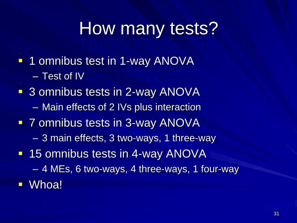
How many tests?
1 omnibus test in 1-way ANOVA
– Test of IV
3 omnibus tests in 2-way ANOVA
– Main effects of 2 IVs plus interaction
7 omnibus tests in 3-way ANOVA
– 3 main effects, 3 two-ways, 1 three-way
15 omnibus tests in 4-way ANOVA
– 4 MEs, 6 two-ways, 4 three-ways, 1 four-way
Whoa!

32

33
time for a new (quasi)experiment
A test of the “Reinforcement Sensitivity Theory” of personality:
some researchers have suggested that our personality is related to our capacity to learn from reward and punishment.
people with an impulsive personality learn well from reward but not punishment, and people with an anxious personality learn well from punishment but not reward.
possible gender differences are not clearly understood
we construct a basic point-scoring reaction-time task measuring reactions time (RT) to investigate this theory– reward for fast responses or punishment for slow responses, plus a
control condition where no reward/punishment is given
– ½ of the participants have an anxious personality, ½ have an impulsive personality
– ½ are male, ½ are female

34
time for a new (quasi)experiment
there are a number of effects which might emerge:– main effects:
• reinforcement (reward, punishment, none)
• personality (impulsive, anxious)
• gender (male, female)
– two-way interactions (also called first-order interactions):
• reinforcement x personality
• reinforcement x gender
• personality x gender
– three-way interaction (also called second-order interaction):
• reinforcement x personality x gender

35
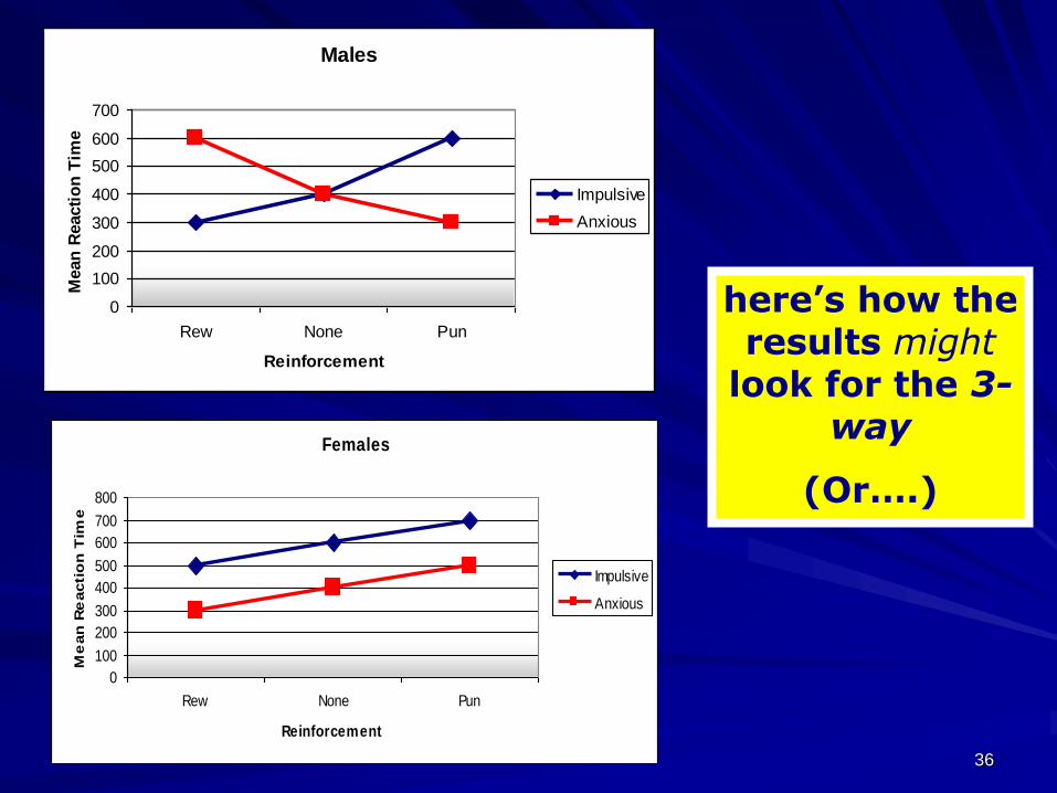
meanings of effects in 3-way
designs main effects:
– differences between marginal means of one factor (averaging over levels of other factors)
two-way interactions:– examines whether the effect of one factor is the same
at every level of another factor
(averaging over levels of a third factor)
three-way interaction:– examines whether the two-way interaction between
two factors is the same at every level of the third factor
36
here’s how the results might
look for the 3-way
(Or….)
Females
0
100
200
300
400
500
600
700
800
Rew None Pun
Reinforcement
Me
an
Re
acti
on
Tim
e
Impulsive
Anxious
Males
0
100
200
300
400
500
600
700
Rew None Pun
Reinforcement
Mean
Reacti
on
Tim
e
Impulsive
Anxious

37
Note on hand calculations for the
three-way
You will not be assessed on them– For the rest of your career you will generally use
SPSS or another stats package (tho‟ sometimes you can end up doing follow-ups / simple effects / simple comparisons by hand)
Formulae plus example of hand calculations for three-way are posted in the resources section of the web site for you to look at
However, you do need to know & understand the degrees of freedom for each effect (which means are being compared)

38
data and cell totals/means
(full layout)Males
Personality Rew None Pun
Impulsive 310 355 490
320 350 495
330 360 485
Total 960 1065 1470
Mean 320 355 490
Anxious 485 450 310
490 455 320
495 445 330
Total 1470 1350 960
Mean 490 450 320
Reinforcement
Females
Personality Rew None Pun
Impulsive 310 450 490
320 455 486
330 445 480
Total 960 1350 1456
Mean 320 450 485
Anxious 485 345 310
480 350 320
490 355 330
Total 1455 1050 960
Mean 485 350 320
Reinforcement

39
degrees of freedom
dftotal = N-1 = 36 -1 = 35
dfP = p-1 = 2 -1 = 1
dfG = g-1 = 2 -1 = 1
dfR = r-1 = 3 -1 = 2
dfPG = (p-1)(g-1) = 1 x 1 = 1
dfRG = (r-1)(g-1) = 2 x 1 = 2
dfPR = (p-1)(r-1) = 1 x 2 = 2
dfPRG = (p-1)(g-1)(r-1) = 1 x 1 x 2 = 2
dferror = N-prg = 36 - 2 x 3 x 2 = 36 – 12 = 24
Regardless of # of factors in
between-groups design, df for a
factor always = # of levels - 1
Df for an interaction
always multiply df for
factors involved
Df for error always N - #cells or (n-1) x
(# cells)
40
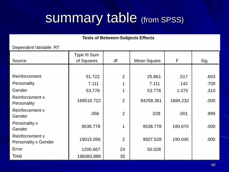
summary table (from SPSS)
Tests of Between-Subjects Effects
Dependent Variable: RT
51.722 2 25.861 .517 .603
7.111 1 7.111 .142 .709
53.778 1 53.778 1.075 .310
168516.722 2 84258.361 1684.232 .000
.056 2 .028 .001 .999
9538.778 1 9538.778 190.670 .000
19015.056 2 9507.528 190.045 .000
1200.667 24 50.028
198383.889 35
Source
Reinforcement
Personality
Gender
Reinforcement x
Personality
Reinforcement x
Gender
Personality x
Gender
Reinforcement x
Personality x Gender
Error
Total
Type III Sum
of Squares df Mean Square F Sig.

41
no significant main effects
Tests of Between-Subjects Effects
Dependent Variable: RT
51.722 2 25.861 .517 .603
7.111 1 7.111 .142 .709
53.778 1 53.778 1.075 .310
168516.722 2 84258.361 1684.232 .000
.056 2 .028 .001 .999
9538.778 1 9538.778 190.670 .000
19015.056 2 9507.528 190.045 .000
1200.667 24 50.028
198383.889 35
Source
Reinforcement
Personality
Gender
Reinforcement x
Personality
Reinforcement x
Gender
Personality x
Gender
Reinforcement x
Personality x Gender
Error
Total
Type III Sum
of Squares df Mean Square F Sig.

42
a significant 2-way interaction between
personality and reinforcementTests of Between-Subjects Effects
Dependent Variable: RT
51.722 2 25.861 .517 .603
7.111 1 7.111 .142 .709
53.778 1 53.778 1.075 .310
168516.722 2 84258.361 1684.232 .000
.056 2 .028 .001 .999
9538.778 1 9538.778 190.670 .000
19015.056 2 9507.528 190.045 .000
1200.667 24 50.028
198383.889 35
Source
Reinforcement
Personality
Gender
Reinforcement x
Personality
Reinforcement x
Gender
Personality x
Gender
Reinforcement x
Personality x Gender
Error
Total
Type III Sum
of Squares df Mean Square F Sig.

43
0100
200300
400500
600
Rew Neut Pun
Task condition
Me
an
re
ac
tio
n t
ime
Imp
Anx

44
a significant 2-way interaction between
personality and genderTests of Between-Subjects Effects
Dependent Variable: RT
51.722 2 25.861 .517 .603
7.111 1 7.111 .142 .709
53.778 1 53.778 1.075 .310
168516.722 2 84258.361 1684.232 .000
.056 2 .028 .001 .999
9538.778 1 9538.778 190.670 .000
19015.056 2 9507.528 190.045 .000
1200.667 24 50.028
198383.889 35
Source
Reinforcement
Personality
Gender
Reinforcement x
Personality
Reinforcement x
Gender
Personality x
Gender
Reinforcement x
Personality x Gender
Error
Total
Type III Sum
of Squares df Mean Square F Sig.

45
360370380390400410420430
Imp Anx
Personality
Me
an
re
ac
tio
n t
ime
Men
Women

46
a significant 3-way interaction between
reinforcement, personality and genderTests of Between-Subjects Effects
Dependent Variable: RT
51.722 2 25.861 .517 .603
7.111 1 7.111 .142 .709
53.778 1 53.778 1.075 .310
168516.722 2 84258.361 1684.232 .000
.056 2 .028 .001 .999
9538.778 1 9538.778 190.670 .000
19015.056 2 9507.528 190.045 .000
1200.667 24 50.028
198383.889 35
Source
Reinforcement
Personality
Gender
Reinforcement x
Personality
Reinforcement x
Gender
Personality x
Gender
Reinforcement x
Personality x Gender
Error
Total
Type III Sum
of Squares df Mean Square F Sig.

47
so there’s this 3-way interaction…
what does that mean??
could be one of the following:
o personality X gender 2-way interaction is different across levels of reinforcement
o reinforcement X personality 2-way interaction is different across levels of gender
o reinforcement X gender 2-way interaction is different across levels of personality
need to focus your investigation1) go back to theory and hypotheses
2) conduct follow-up analyses to test predictions

48
GENDER: 2.00 Female
Reinforcement
PunNeutRew
500
400
300
Personality
Imp
Anx
GENDER: 1.00 Male
Reinforcement
PunNeutRew
500
400
300
Personality
Imp
Anx
Males Females
Reinforcement
PunNeutRew
500
400
300
Personality
Imp
Anx
overall 2-way for
Personality x
Reinforcement …
…is different
at each level
of gender

49

50
following-up a 3-way anova main effects with > 2 levels
– main effect comparisons - t-tests or linear contrasts
– as per 2nd year stats and lecture 3
2-way interactions– simple effects (as per lecture 3)
– then, if simple effects are significant with > 2 levels, follow up with simple comparisons
3-way interactions– simple interaction effects (new!)
– if simple interaction effects are significant, follow up with simple simple effects (new!)
– If simple simple effects are significant, follow up with simple simple comparisons (new!)

51
steps for following-up
a 3-way interaction
is 3-way significant?
NO
calculate simple interaction effects at each level of least
important factor or according to hypotheses
YES
NOYES
does factor A or B have >2 levels?
NO YESconduct tests
for simple simple
comparisons
STOP
STOP
STOP
STOP
is A x B at C1 or C2
significant?
are the simple simple effects of key IV (A or B) significant?
NO
STOP
YES

52
GENDER: 2.00 Female
Reinforcement
PunNeutRew
500
400
300
Personality
Imp
Anx
GENDER: 1.00 Male
Reinforcement
PunNeutRew
500
400
300
Personality
Imp
Anx
Males Females
Reinforcement
PunNeutRew
500
400
300
Personality
Imp
Anx
overall 2-way
Vs simple 2-
way
interactions…
Test 2 way
interaction with
data averaged
across gender

53
simple interaction effectsjust as simple (main) effects are almost exactly the same as examining the 1-way treatment effect on factor A at each level of factor B, simple interaction effects are almost exactly the same as examining the 2-way interaction between factor A and B, at each level of factor C.
What distinguishes simple (main) effects from multiple 1-way anova treatment effects and simple interaction effects from 2-way interactions is that simple main and interaction effects use MSerrorfrom the overall anova as the error term

54
the graphs depicting the 2x2x3 interaction between gender, personality and reinforcement also provide a visual representation of the simple interaction effects
we would conduct – a simple personality x reinforcement interaction at the two levels of gender
GENDER: 2.00 Female
Reinforcement
PunNeutRew
500
400
300
Personality
Imp
Anx
GENDER: 1.00 Male
Reinforcement
PunNeutRew
500
400
300
Personality
Imp
Anx
Males Females

55
Males
Personality Rew None Pun
Impulsive 310 355 490
320 350 495
330 360 485
Total 960 1065 1470
Mean 320 355 490
Anxious 485 450 310
490 455 320
495 445 330
Total 1470 1350 960
Mean 490 450 320
Reinforcement
Females
Personality Rew None Pun
Impulsive 310 450 490
320 455 486
330 445 480
Total 960 1350 1456
Mean 320 450 485
Anxious 485 345 310
480 350 320
490 355 330
Total 1455 1050 960
Mean 485 350 320
Reinforcement
so does the original data table– this is just what we would have if we ran 2 separate 2-way anovas

56
Males
Personality Rew None Pun Marginal
Impulsive 310 355 490
320 350 495
330 360 485
Total 960 1065 1470 3495
Mean 320 355 490
Anxious 485 450 310
490 455 320
495 445 330
Total 1470 1350 960 3780
Mean 490 450 320
Marginal 2430 2415 2430
Totals 7275
Reinforcement
so…in the case
of examining the
two way
interaction
between
Personality and
Reinforcement
FOR MALES, it is
just as if we had
no females in the
study:

57
simple interaction effects
But F tests for simple interaction effects are not
the same as F tests for 2-way interactions
overall personality X reinforcement 2-way interactions:
• MSerror separate value for men and women (taken from each
2-way omnibus ANOVA table)
simple personality X reinforcement 2-way interactions:
• MSerror taken from 3-way omnibus ANOVA table

58
Source SS df MS F p
PR at G1 95725.00 2 47862.50 956.72 0.000
PR at G2 91806.78 2 45903.39 917.56 0.000
Error 1200.67 24 50.03
critical F at alpha=.05 (2,24) = 3.40
summary table forsimple interaction effects
Same error & df as original
ANOVA
Calculated by hand (see
web resources) or via
SPSS

59
Source SS df MS F p
PR at G1 95725.00 2 47862.50 956.72 0.000
PR at G2 91806.78 2 45903.39 917.56 0.000
Error 1200.67 24 50.03
critical F at alpha=.05 (2,24) = 3.40
These are your
calculated SS values
Degrees of freedom for a simple
interaction effect are just the df for
the associated interaction
df = dfPR (2-1)(3-1) = 2
SSerror term (and df) is taken from the
main 2 x 2 x 3 anova
Mean Squares and
F values calculated
as per usualIndicates that the personality x reinforcement interaction is significant
for males and females. Each significant simple interaction needs
following up with simple simple effect tests…

60
61
simple simple effects
remember, simple effects examine the effect of factor A at each level of factor B
simple simple effects are exactly the same as ordinary simple effects except the effect of factor A at each level of factor B, is examined at each level of factor C.
again, MSerror from the overall anova is the error term

62
hence, for both males and females, the effect of personality at each level of reinforcement was significant
(although opposite under neutral reinforcement!)
GENDER: 2.00 Female
Reinforcement
PunNeutRew
500
400
300
Personality
Imp
Anx
GENDER: 1.00 Male
Reinforcement
PunNeutRew
500
400
300
Personality
Imp
Anx
Males Females
could also then compute the simple simple effects of reinforcement at
each level of personality (for males and females)…

63
hence, for both males and females, the effect of reinforcement at each level of personality was significant
GENDER: 2.00 Female
Reinforcement
PunNeutRew
500
400
300
Personality
Imp
Anx
GENDER: 1.00 Male
Reinforcement
PunNeutRew
500
400
300
Personality
Imp
Anx
Males Females
could then follow up the simple simple effect of reinforcement with simple
simple comparisons to see which levels of reinforcement differ within each
level of personality (for males and females)….

64
simple simple comparisonsexactly the same as ordinary simple comparisons / contrasts except we compute for each level of a third factor.
the same formula from Lecture 3 can be used:
abNdferror n
MSa
Lt
errorj
2
jj XaL
65
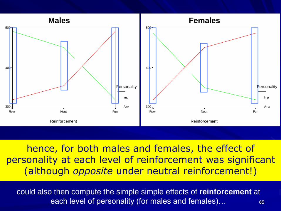
hence, for both males and females, the effect of personality at each level of reinforcement was significant
(although opposite under neutral reinforcement!)
GENDER: 2.00 Female
Reinforcement
PunNeutRew
500
400
300
Personality
Imp
Anx
GENDER: 1.00 Male
Reinforcement
PunNeutRew
500
400
300
Personality
Imp
Anx
Males Females
could also then compute the simple simple effects of reinforcement at
each level of personality (for males and females)…
66
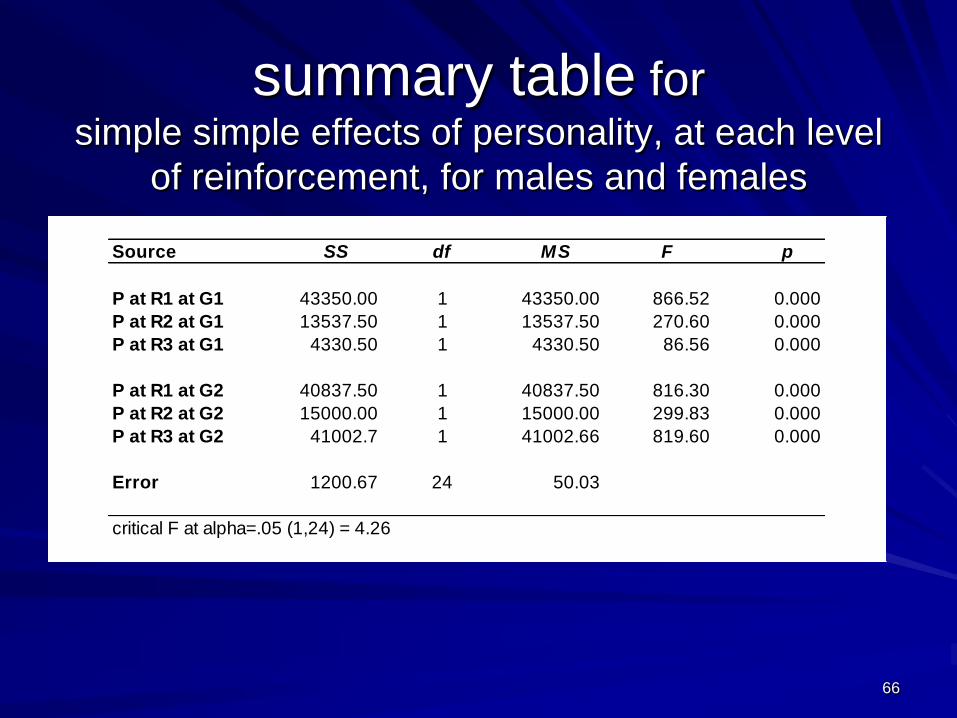
Source SS df MS F p
P at R1 at G1 43350.00 1 43350.00 866.52 0.000
P at R2 at G1 13537.50 1 13537.50 270.60 0.000
P at R3 at G1 4330.50 1 4330.50 86.56 0.000
P at R1 at G2 40837.50 1 40837.50 816.30 0.000
P at R2 at G2 15000.00 1 15000.00 299.83 0.000
P at R3 at G2 41002.7 1 41002.66 819.60 0.000
Error 1200.67 24 50.03
critical F at alpha=.05 (1,24) = 4.26
summary table for simple simple effects of personality, at each level
of reinforcement, for males and females

67
hence, for both males and females, the effect of reinforcement at each level of personality was significant
GENDER: 2.00 Female
Reinforcement
PunNeutRew
500
400
300
Personality
Imp
Anx
GENDER: 1.00 Male
Reinforcement
PunNeutRew
500
400
300
Personality
Imp
Anx
Males Females
could then follow up the simple simple effect of reinforcement with simple
simple comparisons to see which levels of reinforcement differ within each
level of personality (for males and females)….

68
Source SS df MS F p
R at P1 at G1 48350.00 2 24175.00 483.23 0.000
R at P2 at G1 47400.00 2 23700.00 473.74 0.000
R at P1 at G2 45483.56 2 22741.78 454.58 0.000
R at P2 at G2 46350.00 2 23175.00 463.24 0.000
Error 1200.67 24 50.03
critical F at alpha=.05 (2,24) = 3.40
summary tablesimple simple effects of reinforcement, at each
level of personality, for males and females

69
simple simple comparisonsexactly the same as ordinary simple comparisons / contrasts except we compute for each level of a third factor.
the same formula from Lecture 3 can be used:
abNdferror n
MSa
Lt
errorj
2
jj XaL

70
GENDER: 2.00 Female
Reinforcement
PunNeutRew
500
400
300
Personality
Imp
Anx
GENDER: 1.00 Male
Reinforcement
PunNeutRew
500
400
300
Personality
Imp
Anx
Males Females
some possible comparisons…
R1 and R2 vs R3 at P1 for G1 … R2 vs R3 at P2 for G1 …etc

71
Males Rew None Pun
Impusivity 320 355 490
Contrast 1 1 -1 0
Contrast 2 1 1 -2
Anxiety 490 450 320
Contrast 1 1 -1 0
Contrast 2 1 1 -2
Consumption
simple simple comparisons for
reinforcement at each level of
personality (for males)
Note: these are slightly different contrasts to the ones from Lecture 3 –
the exact comparisons you make will depend upon your theory

72
Calculations for impulsivity contrast 1
06.6
3
50.03)0)1(1(
00.35
222
t
L = 2(66.88) – 1(66.88) – 1(35.63) = -35.63
t’=.05 (24) = 2.39
(with Bonferroni adjustment for 2 comparisons)
L = 1(320) – 1(355) + 0(490) = -35.00
Males Rew None Pun
Impusivity 320 355 490
Contrast 1 1 -1 0
Contrast 2 1 1 -2
Anxiety 490 450 320
Contrast 1 1 -1 0
Contrast 2 1 1 -2
Consumption

73
…and so on for
– impulsivity contrast 2…
– Anxiety contrast 1…
– Anxiety contrast 2…
– then all four contrasts
for females…

74
count the number of tests we‟ve
just conducted omnibus tests
– 7 (3 main effects, 3 two-way interactions, 1 three-way interaction)
simple interaction effects– 2 (personality x reinforcement at each level of gender)
simple simple effects– 10 (6 for personality (at each level of reinforcement) for males
and females, 4 for reinforcement (at each level of personality) for males and females)
simple simple comparisons– 8 (2 comparisons for each personality condition
for males and females)
total = 27 tests!!!, – each with a type-1 error rate of .05!!!
– this leads to a familywise error rate of
27*.05 = .7, or 135% (lets just say ‘high’!)

75
take-home message conducting an exhaustive set of follow-up tests for
higher-order factorial designs can inflate familywise alpha (and is very tedious!)
ultimately, there is no simple rule: what you report depends entirely upon your research predictions– in our case we had (implicitly) predicted the Personality x
Reinforcement interaction, and we were going to see if this interaction was the same for males and females
• people with an impulsive personality learn well from reward but not punishment, and people with an anxious personality learn well from punishment but not reward.
• Possible gender differences not well understood.
– hence our write up might have gone something like this…

76
reporting“The predicted interaction was significant, F(2, 24) = 1684.23, p<.001, but this was qualified by 3-way interaction among personality, reinforcement, and gender F(2, 24) = 190.67, p<.001. Simple interaction analyses revealed the personality x reinforcement interaction was significant for both males, F(2, 24) = 956.72, p<.001, and females, F(2, 24) = 917.56, p<.001. The simple simple effects of personality were then analysed for each level of gender and reinforcement, and Table 1 presents the relevant means. For both genders, as predicted, under punishment anxious participants were faster than impulsive participants, Fs > 819.58, ps<.001, while under reward impulsive participants were faster than anxious participants, Fs > 816.29, ps<.001. However, in the neutral reinforcement condition the gender difference emerged: impulsive males performed better than anxious males F(1, 24) = 270.60, p<.001 (Ms = 355, 450), while impulsive females performed worse than anxious females, F(2, 24) = 299.83, p<.001 (Ms = 450, 350).”
I haven‟t put effect sizes. These would be
required for all tests these days.

77
Table 1. Mean reaction time as a function of
personality, reinforcement, and gender. Personality Type
Impulsive Anxious
Reinforcement:
Punishment
Women 485.33a 320.00a
Men 490.00a 320.00a
None
Women 450.00a 350.00a
Men 355.00a 450.00a
Reward
Women 320.00a 485.00a
Men 320.00a 490.00a
Note. Subscripts within the row indicate significant simple simple effects of personality.
Most experimental journals would also want to see standard deviations.

78
steps for following-up
a 3-way interaction
is 3-way significant?
NO
calculate simple interaction effects at each level of least
important factor or according to hypotheses
YES
NOYES
does factor A or B have >2 levels?
NO YESconduct tests
for simple simple
comparisons
STOP
STOP
STOP
STOP
is A x B at C1 or C2
significant?
are the simple simple effects of key IV (A or B) significant?
NO
STOP
YES

79
summary
3-way interactions are very complex!
this increasing complexity highlights the
need for analyses to be driven by your
hypotheses
it also foreshadows the usefulness of
computerised statistical packages like
SPSS (which you will start using in tutes
next week!)

80
Next week:
Power analysis
Readings for this week:
Howell chapter 13– especially section 13.12
Field Chapter 10 (and look through SPSS stuff-i.e. sections 10.3-onwards for next week‟s tutorial!)
Field Chapter 2 (a good introduction to SPSS for the tutes next week)
In the tutes:
This week: Hand calculations for follow-ups
Next week – SPSS tute!