PSYCHOLOGICAL SCIENCE Research Article · PSYCHOLOGICAL SCIENCE Research Article ... Apparatus A diagram of the ... optical lens' equipment of the apparatus, (b) Display of the test-surround

SPHERICAL MODEL OF COLOR AND

BRIGHTNESS DISCRIMINATION Ch.A. Izmailov and E.N. Sokolov

Moscow State University

PSYCHOLOGICAL SCIENCE

Research Article

Abstract - The most important problem confronting color science is the construction of a uniform color space, i.e., a geometrical model of color discrimination in which Euclidean distances between the points representing colors are proportional to perceived color differences. The traditional approach to the construction of a metric color space is based on the integration of just-noticeable color differences (Wyszecki & Stiles, 1982). Experimental data show, however, that the integral of just- noticeable differences between colors does not coincide with direct estimations of the subjective differences between the colors (Judd, 1967; Izmailov, 1980). We suggest another way to construct a uniform color space, namely, to analyze large color differences by multidimensional scaling. This paper reports three groups of experimental data of the measurement of large color differences. Based on these data, we suggest a new color space model taking into account nontraditional relations between threshold and suprathreshold differences. The first group of data includes the results of research on color discrimination for a set of equibright monochromatic lights. The second group includes data on the discrimination of achromatic light stimuli resulting from different relations between test and background luminances. The third group consists of results of color-naming classification of lights varying in chromaticity and brightness. Chromatic differences between spectral stimuli of equal brightness, varying in hue and saturation, and differences in brightness between achromatic lights varying in luminance were analyzed separately. The results are compared with a general color space of colors of different hue, saturation, and brightness. The color spaces were constructed by the same multidimensional scaling technique. An important advantage of multidimensional scaling is that it offers the possibility of finding the dimensionality of a color space directly from experimental data, as we demonstrate for the analysis of color discrimination data for equibright stimuli.

SPHERICAL MODEL FOR CHROMATIC STIMULI

The traditional concept of dimensionality of a chromatic subspace of a color space is based on two sensory characteristics of light: either color hue and saturation, or red-green and blue- yellow color-opponent systems. A typical model describing color discrimination in these terms is the Euclidean plane,

where color hue and saturation are two polar coordinates of a point (horizontal angle and radius), and the opponent systems are two Cartesian coordinates of the same point.

Discrimination data, however, prove the color space to be significantly non-Euclidean. First, local color discrimination data obtained by Mac Adam, and Brown and Mac Adam (see Wyszecki & Stiles, 1982) show that differential sensitivity areas in an equibright color space cannot be represented as a Euclid- ean quadratic form, but only as a surface having a nonzero Gaussian curvature.

Second, research on the relation between barely just noticeable and suprathreshold differences (Judd, 1967; Izmailov, 1980) show the interrelation to be nonlinear due to nonadditivity of color discrimination.

Third, data on large color differences (Shepard and Carroll, 1966; Izmailov, 1980) indicate that global linearity of color discrimination space with respect to perceived differences between colors increases the dimensionality of the Euclidean color space.

Substantial proof of this hypothesis can be found in Shepard and Carroll (1966). These authors consider the problem of finding the dimensionality of the subjective color discrimination space for equiluminance colors. Their theoretical analysis is based on data reported by Boynton and Gordon (1965).

Boynton and Gordon (1965) studied the dependence of color discrimination on stimulus luminance with three normal subjects by a color-naming technique. They presented 23 monochromatic stimuli with wavelength ranging from 440 to 660 nm (at a step of 10 nm) to subjects who were to divide the stimuli into four color classes bearing the names blue, green, yellow, and red. If a stimulus was considered intermediate between two classes, it was given a double name, such as blue-green, with the name of the color perceived as more manifest coming first. Weight was assigned to each class by the following rules: If a stimulus belonged to one class only, the class received the weight 3; if a stimulus had a double name, as in our example with blue-green, then the first class (blue) was given the weight 2 and the second class (green) the weight 1. Stimuli were presented 25 times each. The weighted frequency of the attribution of a stimulus to each class was assumed as a measure of the stimulus subjective estimate. Marking stimulus wavelength on the abscissa axis and the subjective estimate on the ordinate axis, Boynton and Gordon obtained color-naming curves. By changing stimulus luminance at the levels of 100 and 1,000 tro- lands, Boynton and Gordon measured the dependence of color discrimination on brightness.

In order to make the data suitable for multidimensional seal- Address correspondence to Dr. E.N. Sokolov, Marx Avenue, 18/5,

Moscow, USSR 103009.

VOL. 2, NO. 4, JULY 1991 Copyright © 1991 American Psychological Society 249


Spherical Discrimination Model

ing, Shepard and Carroll treated the responses to each stimulus as a naming vector. The vector's components were weighted frequencies of the assigned names. The number of components thus depends on the number of classes, and consequently, all the vectors were four-component. The distance measure between vectors was taken to be the city-block measure in one case, and the Euclidean measure in the other. Distances between all pairs of vectors formed an n(n - l)/2 matrix of distances averaged for three subjects on luminance level 100 tro- lands (n is the number of stimuli). The matrix was processed by several multidimensional scaling techniques. The spatial model was shown to be independent of the chosen distance measure between reaction vectors. The solution was identical when the differences were interpreted in Euclidean metrics and city- block metrics. Moreover, the spatial model did not depend on the multidimensional scaling algorithm. The results led the authors to a conclusion about the rigidity of the color discrimination space structure.

It was found that the dimensionality of the obtained space changed according to the choice of the approximation criterion of interpoint distances to initial distance measures.

When global linearity was postulated for initial distance measures, the minimal dimensionality of the Euclidean space was three. In a three-dimensional space the 23 points representing monochromatic colors were located so that the line connecting points that represent stimuli from the first to the 23rd was a one-dimensional curve with bends in blue, green, and yellow areas.

When the relation between initial data and interpoint distances was required to be globally monotone instead of linear, Shepard and Carroll obtained a two-dimensional space for the same data. The points were located on a curve in this case also, with the same bends in blue, green, and yellow areas. When the condition was changed from a globally monotone relation to a locally monotone one, the points became located on a straight line. The single dimension could be interpreted as a substantial change of wavelength.

Analyzing the data, Shepard and Carroll noticed a reciprocal relation between the simplicity of the spatial presentation of the initial data, and the simplicity of the presentation's connection with the data. The more complex three-dimensional solution has the advantage of a linear relation with initial data, while the simplest solution compensates for its efficiency by a nonlinear relation with data.

There is another substantive criterion for determining the true dimensionality of the subjective space that must be taken into consideration, namely, the neurophysiological interpretation of obtained data. The existence of a single sensory mech- anism with the complicated principles suggested by the one- dimensional solution does not seem probable. Numerous data on the performance of the color analyzer point to the existence of several simple similarly performing mechanisms conforming to the first solution.

The three-dimensional solution meets, however, with seri- ous difficulties in giving a traditional interpretation to subjective characteristics of aperture colors.

Agreement among the various data becomes possible in a spherical color discrimination space obtained by Sokolov, Iz- mailov, and Schonebeck (1982), Izmailov et al. (1989), Izmailov

(1982), and Sokolov and Izmailov (1983). We now present two experimental runs in above-threshold discrimination and their analysis by multidimensional scaling.

Method

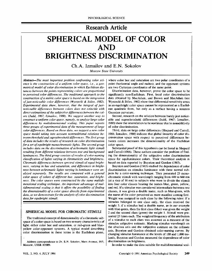
Apparatus A diagram of the apparatus is given in Figure 1. The appa-

ratus consisted of a visual photometer, two tungsten light sources, and a cartridge for quick substitution of Carl Zeiss (Jena) filters. The test circular field subtended about 2°, and the surrounding field subtended about 6°. The visual photometer included a photometric cube and an ocular with Maxwellian

Fig. 1. (a) Schematic representation of the apparatus. R, re- flecting mirrors; P, tungsten sources of light; F^ thermal filters; F2, neutral density filters; F3, F'3, interference spectral filters; W, neutral density wedge; C, photometric glass cube; S, circular diaphragm; L, optical lens' equipment of the apparatus, (b) Display of the test-surround field (disc-ring configuration of stimulus), (c) Spectral transmittance curve for neutral density filters.

250 VOL. 2, NO. 4, JULY 1991


Ch.A. Izmailov and E.N. Sokolov

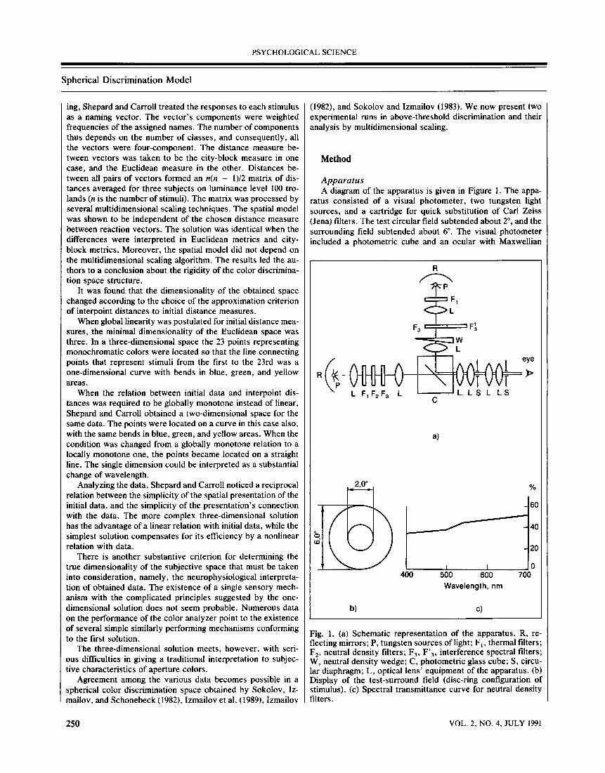
Table 1. Matrix of equibright color differences

nm N 1 2 3 4 5 6 7 8 9 10 11 12 13 14 15 16 17

425 1 12 21 24 28 65 65 68 75 74 75 74 71 68 66 65 60 440 2 14 19 24 61 62 64 73 74 76 76 72 69 68 68 59 450 3 5 16 58 62 62 70 73 76 77 73 70 70 70 57 460 4 10 58 61 61 68 74 77 81 74 73 71 71 54 466 5 56 58 62 69 72 77 79 77 75 73 74 58 520 6 8 27 53 60 68 73 79 84 84 84 59 525 7 25 50 55 63 73 79 83 84 84 57 554 8 39 41 52 68 72 77 77 78 40 570 9 15 33 46 51 62 63 67 30 575 10 26 42 48 61 62 65 52 600 11 29 41 48 50 53 45 613 12 12 27 29 32 53 625 13 17 20 24 60 635 14 4 10 63 650 15 7 64 675 16 66 White 17

view. Luminances of test field and surrounding field were con- trolled by neutral density filters.

Brightness matching The following method was used to equate stimuli brightness.

The luminance and the wavelength of the surrounding field were kept constant (it was neutral light) while the wavelength of central field varied over the whole range of stimuli. Each of the subjects was required to match the brightness of the center to the constant brightness of the surrounding field. Matching data for each test light were averaged over the subjects.

Subjects The subjects were three women aged 18-22 with normal tri-

chromatic color vision, checked by Rabkin's test (Rabkin, 1971). They were instructed to estimate the difference in color between the stimuli using numbers from 0 (complete identity) to 9 (maximum difference from the subject's point of view) and to give their answers as quickly as they could, keeping to their first impression.

Stimuli We used 16 monochromatic lights between 425 and 675 nm,

and one white stimulus created with neutral density film (Fig. lc). Stimuli were presented successively in pairs. Each stimulus was presented during 0.5 s; the interval between stimuli in a pair was 0.5 s and the interval between pairs was 3-5 s. Pairs were presented 10 times each in random order.

Results

The estimates were averaged for every pair and for every subject. The mean of the estimates were brought together in a matrix of pair differences (Table 1). The estimates are given as two-digit numbers, i.e., an integer and one decimal number. From the matrix of subjective differences between colors, the coordinates were calculated using the Torsca multidimensional scaling procedure (Table 2).

Discussion

Dimension of color chromaticity space It turns out that minimal dimensionality of the Euclidean

space for equibright color discriminations is three. The distances between color points in this three-dimensional space correlate highly with the initial estimates of color differences. The correlation coefficient is equal to 0.995. This result must be considered in more detail, because it is proposed traditionally that only two dimensions are sufficient for spacing chromatic- ities of colors. Such a solution can be easily obtained by the projection of all points on the XXX2 plane (see Fig. 2a) or R (675 nm) G (525 nm) B (440 nm) plane. Indeed, all the points pro-

Table 2. Coordinates of color points in the three- dimensional Euclidean space, and characteristics of sphericity (radii, mean radius, standard deviation, etc.)

N nm Xx X2 X3 R

1 425 10.5 -43.0 13.4 46.2 2 440 4.2 -42.4 13.4 44.7 3 450 -3.4 -42.3 17.0 45.7 4 460 -5.8 -43.8 20.2 48.6 5 466 -10.9 -41.2 18.4 46.4 6 520 -36.6 5.5 14.1 39.6 7 525 -35.7 8.4 18.0 40.9 8 554 -24.9 14.4 28.5 40.1 9 570 -5.0 21.4 43.1 48.4

10 575 3.1 22.8 45.8 51.2 11 600 16.7 22.2 33.5 43.5 12 613 32.6 18.8 17.0 41.3 13 625 39.5 13.7 13.5 43.9 14 635 44.0 8.0 6.6 45.2 15 650 44.5 6.0 5.9 45.3 16 675 43.7 3.8 3.1 44.0 17 White 0.5 -0.6 51.2 51.2 Mean radius 45.1 Standard deviation 3.5 Coefficient of variance, % 7.8 Coefficient of correlation 0.995

VOL. 2, NO. 4, JULY 1991 251



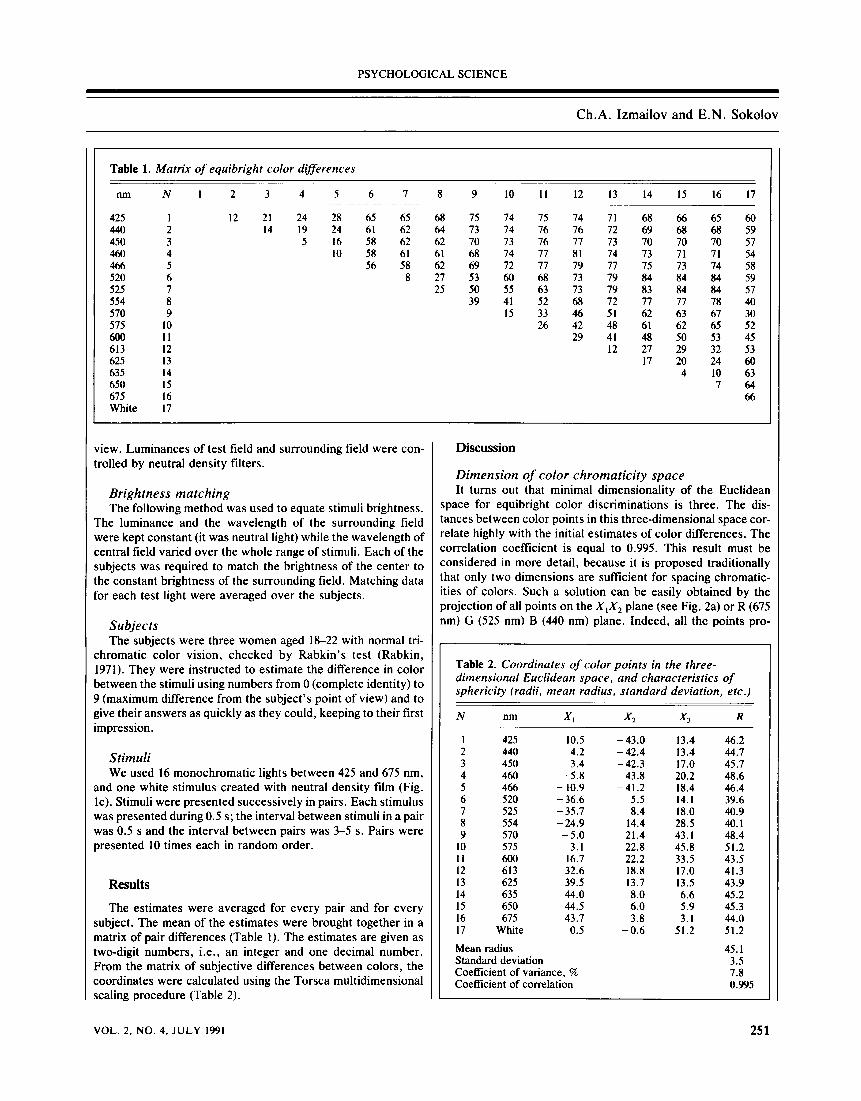
Fig. 2. (a) Projections of color points on the XXX2 coordinates plane for equibright spectrum. White color point is projected near the center of XXX2 plane, (b) Projections of the same color points on the XXX3 coordinates plane for equibright spectrum. White color point has the greatest height, red colors (634-675 nm) have lesser heights.

jected on this plane are in full accordance with the color mixture laws. Besides, the color points are situated in the plane, as can be expected from traditional color models with hue and saturation considered in polar frame of reference. Thus, projection of the obtained structure of color points into the two-dimensional space gives a traditional solution.

However, if this two-dimensional solution is evaluated from the uniformity point of view, a considerable discrepancy is found. The two-dimensional solution has a smaller linear correlation between perceived color differences and interpoint distances.

It seems at first that such a discrepancy could be explained by idealizing the experimental data, putting the distances from the points to the RGB plane (height) equal to zero, while due to some random errors the height of color points must be distrib- uted accidentally in the vicinity of zero. However, as we can

see from the obtained data (Fig. 2b), the spatial distribution of the points around RGB plane is not random. Moreover, the location of the points correlate with the color saturation. Mostly saturated colors - indigo, green, and red - have minimal heights. The less-saturated colors - green-yellow, yellow, orange - have the larger height, reaching the maximum at the white color point. These facts testify that the third dimension is important for color discrimination description.

Three-dimensionality of color-point configuration changes the traditional interpretation of color saturation to some extent. With the diminishing of saturation, the color point shifts in two directions simultaneously - towards the center of color triangle RGB in the XXX2 plane and away from the plane XXX2 itself. It means that it is necessary to use two Cartesian axes to describe the saturation changes in Euclidean space, as is customary, for hue changes description. Radial direction of the XXX2 axes plane, which is interpreted in two-dimensional models as the only characteristic of saturation, is, in fact, one of the axes, while the second one corresponds to the third axis in the three- dimensional space, obtained by MDS analysis.

Equibright colors are represented on a hemisphere, that is, a two-dimensional surface within a three-dimensional space in this representation, but hue and saturation are special cases. Hue is characterized by a horizontal angle and saturation by a vertical angle.

The structure of color points shown in Figure 2 leads to a new interpretation of color opponency, too. Two Cartesian axes of three-dimensional space determining color hue are interpreted in the traditional way as red-green and yellow-blue opponent characteristics, while the third Cartesian axis is interpreted as new achromatic nonbrightness characteristic. Thus, even for equibright colors described in Euclidean terms, it is necessary to use three dimensions.

Color space rotation The choice of particular direction of Cartesian axes requires

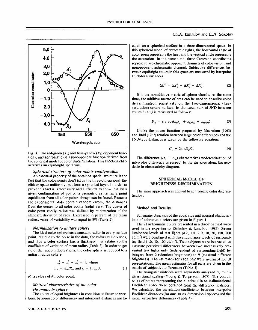
some additional information because interpoint distances are invariant with respect to orthogonal rotation. The phenomena of constant hue and color opponency were used to orient the axes of color space. Configuration of color points is rotated in such a way that the first axis (A',) passes through the point having a constant green (500 nm) hue, the second axis (Ay passes through the points having constant blue (470 nm) and constant yellow (575 nm) hues, and the third axis (X3) passes through the point representing white color. The obtained frame of references represented fundamental opponent characteristics of color vision. The opponent colors function derived from final configuration are shown in Figure 3.

The coordinates Xx and X2 as function of wavelength can be compared with corresponding red-green and blue-yellow functions, constructed by the cancellation technique (Hurvich & Jameson, 1957) and can be interpreted as two opponent neuronal channels of color vision (De Valois, 1973; Zrenner, 1983). The third X3 coordinate of obtained color space represents the achromatic component (desaturation) of color. It can't be compared with well-known white-black color function because the first one represents spectral colors of equal brightness. It can't be interpreted either as a traditional achromatic neuronal channel, which usually is connected with spectral sensitivity curve.

252 VOL. 2, NO. 4, JULY 1991



Fig. 3. The red-green (Xx) and blue-yellow (X2) opponent functions, and achromatic (X3) nonopponent function derived from the spherical model of color discrimination. This function characterizes an equibright spectrum.

Spherical structure of color-points configuration An essential property of the obtained spatial structure is the

fact that the color points don't fill in the three-dimensional Eu- clidean space uniformly, but form a spherical layer. In order to prove this fact it is necessary and sufficient to show that for a given configuration of points, a geometric center as a point equidistant from all color points always can be found. Because the experimental data contain random errors, the distances from the center to all color points (radii) vary. The center of color-point configuration was defined by minimization of the standard deviation of radii. Expressed in percent of the mean radius, value of variability was equal to 8% (Table 2).

Normalization to unitary sphere The ideal color sphere has a constant radius in every surface

point, but due to the noise in the data, the radius value varies, and thus a color surface has a thickness that relates to the coefficient of variation of mean radius (Table 2). In order to get rid of the random fluctuations, the color sphere is reduced to a unitary radius sphere:

*i + xl + xl = 1> where xik = XikIRit and k = 1,2, 3. (1)

Rj is radius of ith color point.

Metrical characteristics of the color chromaticity sphere The colors of equal brightness in condition of linear connec-

tions between color differences and interpoint distances are lo-

cated on a spherical surface in a three-dimensional space. In this spherical model of chromatic lights, the horizontal angle of color point represents the hue, and the vertical angle represents the saturation. In the same time, three Cartesian coordinates represent two chromatic opponent channels of color vision, and nonopponent achromatic channel. Subjective differences between equibright colors in this space are measured by interpoint Euclidean distances:

AC2 = A*2 + AXJ + A*2. (2)

It is the nonadditive metric of sphere chords. At the same time, the additive metric of arcs can be used to describe color discrimination sensitivity on the two-dimensional (hue- saturation) sphere surface. In this case, sum of JND between colors / andy is measured as follows:

Du = arc cosC*,,*,! + x^cn + x^x^). (3)

Unlike the power function proposed by MacAdam (1963) and Judd (1967) relation between large color differences and the JND-type distances is given by the following equation:

Cu = 2sin/y2. (4)

The difference (Do - Co) characterizes underestimation of intercolor difference in respect to the distance along the geodesic in chromaticity diagram.

SPHERICAL MODEL OF BRIGHTNESS DISCRIMINATION

The same approach was applied to achromatic color discrimination.

Method and Results

Schematic diagrams of the apparatus and spectral characteristic of achromatic colors are given in Figure 1 .

The 21 achromatic colors presented in a disc-ring field were used in the experiments (Sokolov & Izmailov, 1984). Seven luminance levels of test lights (0.2, 1.0, 2.0, 10, 20, 100, 200 cd/m2) were combined with three luminance levels of surrounding field (1.0, 10, 100 cd/m2). Two subjects were instructed to estimate perceived differences between two successively presented test lights only (independent of surrounding field) by integers from 0 (identical brightness) to 9 (maximal different brightness). The estimates for each pair were averaged for 10 presentations. The mean estimates for all pairs are given in the matrix of subjective differences (Table 3).

The triangular matrices were separately analyzed by multidimensional scaling (Young & Torgerson, 1967). The coordinates of points representing the 21 stimuli in an /z-dimensional Euclidean space were obtained from the difference matrices. We calculated the correlation coefficients between interpoint Euclidean distances (for one- to six-dimensional spaces) and the initial subjective differences (Table 4).

VOL. 2, NO. 4, JULY 1991 253



Table 3. Estimates of perceived differences between test achromatic colors, summarized from 10 presentations of each pair

Back- Test ground

Lumi- Lumi- nance nance

(cd/m2) (cd/m2) N 1 2 3 4 5 6 7 8 9 10 11 12 13 14 15 16 17 18 19 20 21

0.2 100 1 1 23 0 12 30 8 28 44 18 34 47 50 52 54 60 47 63 63 63 64 0.2 10 2 19 18 2 4 34 11 15 42 17 19 44 44 46 45 51 52 56 62 58 62 0.2 1 3 42 24 20 12 14 11 4 25 7 17 29 23 45 28 40 43 37 51 52 48 1 100 4 10 14 25 6 32 6 16 44 11 35 48 41 55 49 55 59 60 62 61 61 1 10 5 28 7 17 27 22 9 12 40 15 29 41 41 44 45 46 48 49 56 53 59 1 1 6 44 35 29 40 38 22 11 11 12 7 12 13 10 13 38 35 22 34 33 31 2 100 7 13 12 31 10 17 28 6 34 8 31 43 34 40 41 47 52 53 58 56 59 2 10 8 36 32 19 33 7 11 13 13 7 15 18 22 33 26 31 31 47 45 48 48 2 1 9 62 60 23 61 45 19 41 38 29 4 3 11 3 6 22 18 20 28 29 30

10 100 10 22 20 11 21 14 14 14 12 31 8 29 26 31 31 40 38 37 56 51 47 10 10 11 50 38 31 49 42 18 39 23 20 23 10 8 11 11 23 24 23 30 27 30 10 1 12 73 70 44 72 68 28 63 39 12 30 12 8 6 5 11 13 26 24 26 26 20 100 13 51 38 21 43 24 17 35 13 13 24 18 19 7 3 15 15 19 25 29 23 20 10 14 72 72 57 76 68 25 66 39 15 46 12 15 24 3 14 13 5 23 22 24 20 1 15 77 74 59 70 72 28 68 51 18 46 30 20 30 8 14 14 15 27 23 20

100 100 16 88 85 71 84 80 41 77 66 20 68 24 14 57 14 10 6 6 11 19 20 100 10 17 87 85 71 85 83 44 74 73 29 69 35 19 47 12 11 7 7 21 17 18 100 1 18 86 80 77 84 79 58 77 64 28 76 42 24 51 19 12 8 10 18 11 10 200 100 19 90 88 75 88 85 59 81 64 36 71 45 21 54 22 18 12 7 9 12 200 10 20 90 89 72 86 82 50 80 67 39 67 38 26 66 25 21 13 9 10 3 2 200 1 21 89 88 76 88 84 55 75 69 38 75 48 28 67 26 23 15 6 7 5 0

Note. Upper right triangle of the matrix represents the data of subject IP, and bottom left triangle of the matrix represents the data of subject KN.

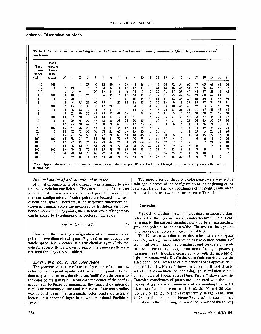
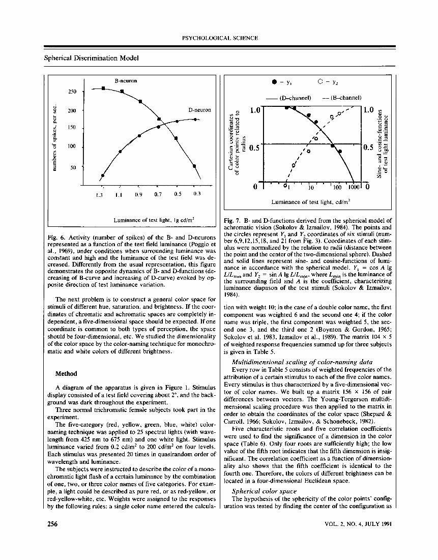
Dimensionality of achromatic color space The coordinates of achromatic color points were adjusted by Minimal dimensionality of the spaces was estimated by sat- shifting the center of the configuration to the beginning of the

urating correlation coefficients. The correlation coefficients as reference frame. The new coordinates of the points, radii, mean a function of dimensions are shown in Figure 4. It was found radii, and standard deviations are given in Table 4. that our configurations of color points are located in a two- dimensional space. Therefore, if the subjective differences between achromatic colors are measured by Euclidean distances Discussion between corresponding points, the different levels of brightness _. „ , t t. n. . t ., can be coded by two-dimensional vectors in the space: Fl8ure _. 5 „ shows , that t stimuh t. of n. ̂creasing

. t brightness ., are characterized by the angle measured counterclockwise. Point 1 cor-

22 2 /ca responds to the darkest stimulus, point 11 to an intermediate 12 * /ca ' grey, and point 21 to the best white. The test and background

luminances of all colors are given in Table 3. However, the resulting configuration of achromatic color The Cartesian coordinates of this achromatic color space

points in two-dimensional space (Fig. 5) does not occupy the (axes Yj and ̂ can be interpreted as two neuron channels of whole space, but is located in a semicircular layer. (Only the the visual system known as brightness and darkness channels data for subject IP are shown in Fig. 5; the same results were (B_ and D.ceUs) (Jung 1973)> or on_ and off-cells, respectively obtained for subject KN, Table 4.) (Zrenner, 1983). B-cells increase activity with the increase of

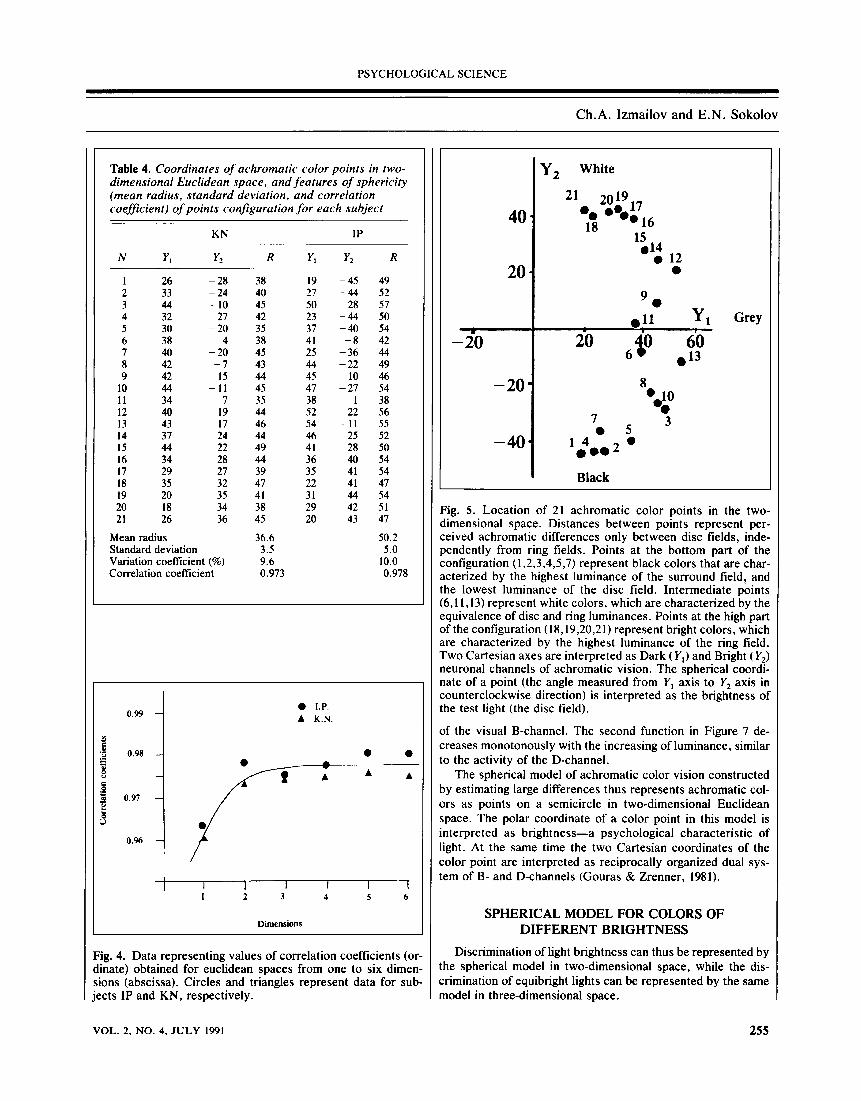
light luminance, while D-cells decrease their activity under the Sphericity of achromatic color space same conditions. Decrease of luminance evokes opposite reac- The geometrical center of the configuration of achromatic tions of the cells. Figure 6 shows the curves of B- and D-cells'

color points is a point equidistant from all color points. As the activity in the conditions of decreasing light stimulation as built data may contain errors, the distances (radii) from the center to up from data of Poggio et al. (1969). Figure 7 shows how the the color points may vary. In our case the center of the config- Cartesian coordinates of points are connected with the lumi- uration can be found by minimizing the standard deviation of nances of test stimuli. Luminance of surrounding field is 1.0 radii. The variability of the radii in percent of the mean radius cd/m2, test field luminances are 1, 2, 10, 20, 100, and 200 cd/m2 was 10%. It means that achromatic color points are actually (points 6, 9, 12, 15, 18, and 21 respectively, in Fig. 5 and Table located in a spherical layer in a two-dimensional Euclidean 4). One of the functions in Figure 7 (circles) increases monot- space. onously with the increasing of luminance, similar to the activity

254 VOL. 2, NO. 4, JULY 1991



Table 4. Coordinates of achromatic color points in two- dimensional Euclidean space, and features of sphericity (mean radius, standard deviation, and correlation coefficient) of points configuration for each subject

KN IP

N Yl Y2 R K, Y2 R

1 26 -28 38 19 -45 49 2 33 -24 40 27-44 52 3 44 -10 45 50-28 57 4 32 -27 42 23-44 50 5 30 -20 35 37 -40 54 6 38 4 38 41 -8 42 7 40 -20 45 25 -36 44 8 42 -7 43 44 -22 49 9 42 15 44 45 10 46

10 44 -11 45 47 -27 54 11 34 7 35 38 1 38 12 40 19 44 52 22 56 13 43 17 46 54-11 55 14 37 24 44 46 25 52 15 44 22 49 41 28 50 16 34 28 44 36 40 54 17 29 27 39 35 41 54 18 35 32 47 22 41 47 19 20 35 41 31 44 54 20 18 34 38 29 42 51 21 26 36 45 20 43 47

Mean radius 36.6 50.2 Standard deviation 3.5 5.0 Variation coefficient {%) 9.6 10.0 Correlation coefficient 0.973 0.978

Fig. 4. Data representing values of correlation coefficients (ordinate) obtained for euclidean spaces from one to six dimensions (abscissa). Circles and triangles represent data for subjects IP and KN, respectively.

Fig. 5. Location of 21 achromatic color points in the two- dimensional space. Distances between points represent perceived achromatic differences only between disc fields, inde- pendently from ring fields. Points at the bottom part of the configuration (1,2,3,4,5,7) represent black colors that are characterized by the highest luminance of the surround field, and the lowest luminance of the disc field. Intermediate points (6,1 1,13) represent white colors, which are characterized by the equivalence of disc and ring luminances. Points at the high part of the configuration (18,19,20,21) represent bright colors, which are characterized by the highest luminance of the ring field. Two Cartesian axes are interpreted as Dark (Yx) and Bright (Y2) neuronal channels of achromatic vision. The spherical coordinate of a point (the angle measured from Yx axis to Y2 axis in counterclockwise direction) is interpreted as the brightness of the test light (the disc field). of the visual B-channel. The second function in Figure 7 de- creases monotonously with the increasing of luminance, similar to the activity of the D-channel.

The spherical model of achromatic color vision constructed by estimating large differences thus represents achromatic colors as points on a semicircle in two-dimensional Euclidean space. The polar coordinate of a color point in this model is interpreted as brightness - a psychological characteristic of light. At the same time the two Cartesian coordinates of the color point are interpreted as reciprocally organized dual system of B- and D-channels (Gouras & Zrenner, 1981).

SPHERICAL MODEL FOR COLORS OF DIFFERENT BRIGHTNESS

Discrimination of light brightness can thus be represented by the spherical model in two-dimensional space, while the discrimination of equibright lights can be represented by the same model in three-dimensional space.

VOL. 2, NO. 4, JULY 1991 255



Fig. 6. Activity (number of spikes) of the B- and D-neurons represented as a function of the test field luminance (Poggio et al., 1969), under conditions when surrounding luminance was constant and high and the luminance of the test field was de- creased. Differently from the usual representation, this figure demonstrates the opposite dynamics of B- and D-functions (decreasing of B-curve and increasing of D-curve) evoked by opposite direction of test luminance variation.

Fig. 7. B- and D-functions derived from the spherical model of achromatic vision (Sokolov & Izmailov, 1984). The points and the circles represent Yx and Y2 coordinates of six stimuli (number 6,9,12,15,18, and 21 from Fig. 3). Coordinates of each stimulus were normalized by the relation to radii (distance between the point and the center of the two-dimensional sphere). Dashed and solid lines represent sine- and cosine-functions of luminance in accordance with the spherical model. Yx = cos A lg L/Lmin and Y2 = sin A lg L/Lmin, where Lmin is the luminance of the surrounding field and A is the coefficient, characterizing luminance diapason of the test stimuli (Sokolov & Izmailov, 1984). The next problem is to construct a general color space for

stimuli of different hue, saturation, and brightness. If the coordinates of chromatic and achromatic spaces are completely independent, a five-dimensional space should be expected. If one coordinate is common to both types of perception, the space should be four-dimensional, etc. We studied the dimensionality of the color space by the color-naming technique for monochromatic and white colors of different brightness.

Method

A diagram of the apparatus is given in Figure 1 . Stimulus display consisted of a test field covering about 2°, and the background was dark throughout the experiment.

Three normal trichromatic female subjects took part in the experiment.

The five-category (red, yellow, green, blue, white) color- naming technique was applied to 25 spectral lights (with wavelength from 425 nm to 675 nm) and one white light. Stimulus luminance varied from 0.2 cd/m2 to 200 cd/m2 on four levels. Each stimulus was presented 20 times in quasirandom order of wavelength and luminance.

The subjects were instructed to describe the color of a monochromatic light flash of a certain luminance by the combination of one, two, or three color names of five categories. For example, a light could be described as pure red, or as red-yellow, or red-yellow- white, etc. Weights were assigned to the responses by the following rules: a single color name entered the calcula-

tion with weight 10; in the case of a double color name, the first component was weighted 6 and the second one 4; if the color name was triple, the first component was weighted 5, the second one 3, and the third one 2 (Boynton & Gordon, 1965; Sokolov et al. 1983, Izmailov et al., 1989). The matrix 104 x 5 of weighted response frequencies summed up for three subjects is given in Table 5.

Multidimensional scaling of color-naming data Every row in Table 5 consists of weighted frequencies of the

attribution of a certain stimulus to each of the five color names. Every stimulus is thus characterized by a five-dimensional vector of color names. We built up a matrix 156 x 156 of pair differences between vectors. The Young-Torgerson multidimensional scaling procedure was then applied to the matrix in order to obtain the coordinates of the color space (Shepard & Carroll, 1966; Sokolov, Izmailov, & Schonebeck, 1982).

Five characteristic roots and five correlation coefficients were used to find the significance of a dimension in the color space (Table 6). Only four roots are sufficiently high; the low value of the fifth root indicates that the fifth dimension is insig- nificant. The correlation coefficient as a function of dimensionality also shows that the fifth coefficient is identical to the fourth one. Therefore, the colors of different brightness can be located in a four-dimensional Euclidean space.

Spherical color space The hypothesis of the sphericity of the color points' config-

uration was tested by finding the center of the configuration as

256 VOL. 2, NO. 4, JULY 1991



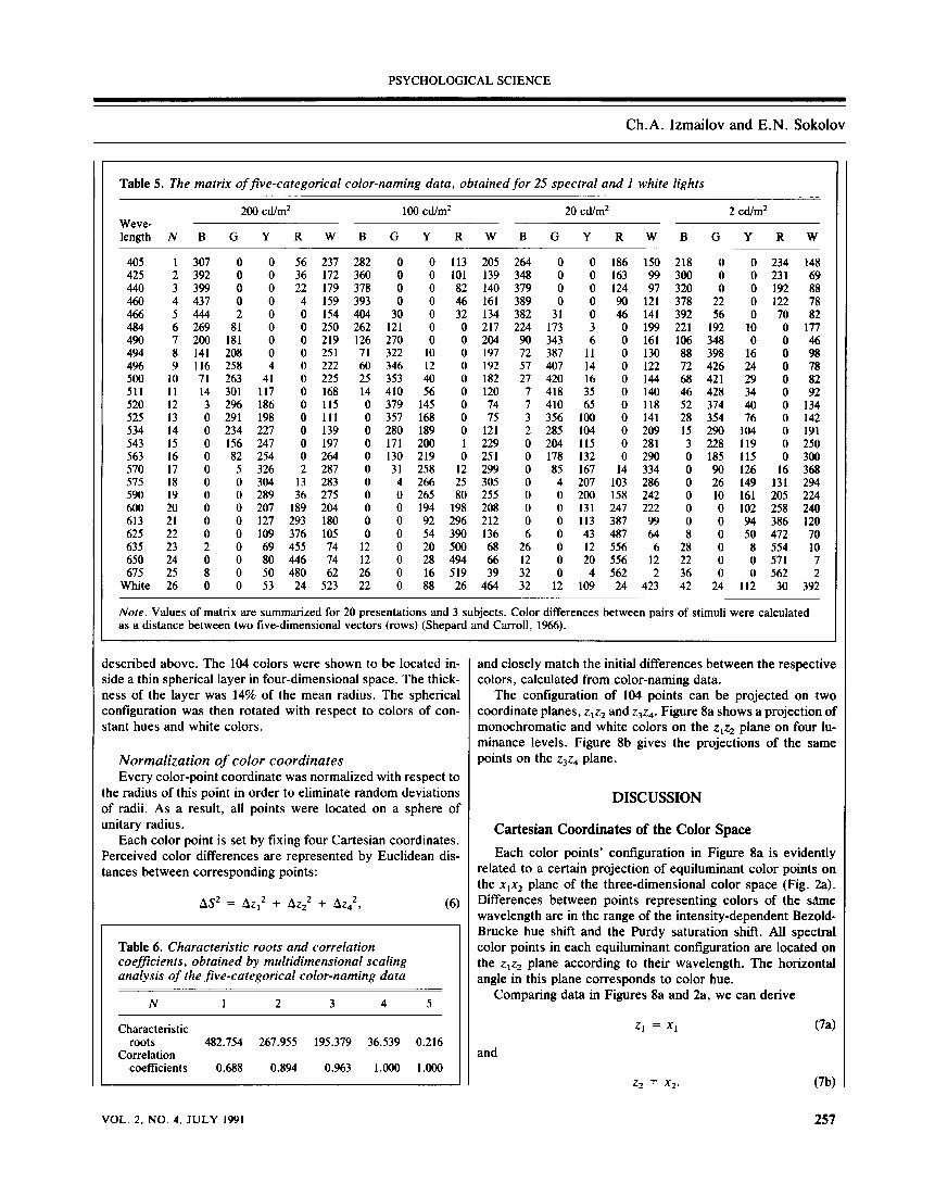
Table 5. The matrix of five-categorical color-naming data, obtained for 25 spectral and 1 white lights 200cd/m2 100cd/m2 20 cd/m2 2 cd/m2

Weve- length NBGYRWBGYRWBGYRWBGYRW

405 1 307 0 0 56 237 282 0 0 113 205 264 0 0 186 150 218 0 0 234 148 425 2 392 0 0 36 172 360 0 0 101 139 348 0 0 163 99 300 0 0 231 69 440 3 399 0 0 22 179 378 0 0 82 140 379 0 0 124 97 320 0 0 192 88 460 4 437 0 0 4 159 393 0 0 46 161 389 0 0 90 121 378 22 0 122 78 466 5 444 2 0 0 154 404 30 0 32 134 382 31 0 46 141 392 56 0 70 82 484 6 269 81 0 0 250 262 121 0 0 217 224 173 3 0 199 221 192 10 0 177 490 7 200 181 0 0 219 126 270 0 0 204 90 343 6 0 161 106 348 0 0 46 494 8 141 208 0 0 251 71 322 10 0 197 72 387 11 0 130 88 398 16 0 98 496 9 116 258 4 0 222 60 346 12 0 192 57 407 14 0 122 72 426 24 0 78 500 10 71 263 41 0 225 25 353 40 0 182 27 420 16 0 144 68 421 29 0 82 511 11 14 301 117 0 168 14 410 56 0 120 7 418 35 0 140 46 428 34 0 92 520 12 3 296 186 0 115 0 379 145 0 74 7 410 65 0 118 52 374 40 0 134 525 13 0 291 198 0 111 0 357 168 0 75 3 356 100 0 141 28 354 76 0 142 534 14 0 234 227 0 139 0 280 189 0 121 2 285 104 0 209 15 290 104 0 191 543 15 0 156 247 0 197 0 171 200 1 229 0 204 115 0 281 3 228 119 0 250 563 16 0 82 254 0 264 0 130 219 0 251 0 178 132 0 290 0 185 115 0 300 570 17 0 5 326 2 287 0 31 258 12 299 0 85 167 14 334 0 90 126 16 368 575 18 0 0 304 13 283 0 4 266 25 305 0 4 207 103 286 0 26 149 131 294 590 19 0 0 289 36 275 0 0 265 80 255 0 0 200 158 242 0 10 161 205 224 600 20 0 0 207 189 204 0 0 194 198 208 0 0 131 247 222 0 0 102 258 240 613 21 0 0 127 293 180 0 0 92 2% 212 0 0 113 387 99 0 0 94 386 120 625 22 0 0 109 376 105 0 0 54 390 136 6 0 43 487 64 8 0 50 472 70 635 23 2 0 69 455 74 12 0 20 500 68 26 0 12 556 6 28 0 8 554 10 650 24 0 0 80 446 74 12 0 28 494 66 12 0 20 556 12 22 0 0 571 7 675 25 8 0 50 480 62 26 0 16 519 39 32 0 4 562 2 36 0 0 562 2

White 26 0 0 53 24 523 22 0 88 26 464 32 12 109 24 423 42 24 112 30 392

Note. Values of matrix are summarized for 20 presentations and 3 subjects. Color differences between pairs of stimuli were calculated as a distance between two five-dimensional vectors (rows) (Shepard and Carroll, 1966).

described above. The 104 colors were shown to be located in- side a thin spherical layer in four-dimensional space. The thickness of the layer was 14% of the mean radius. The spherical configuration was then rotated with respect to colors of constant hues and white colors.

Normalization of color coordinates Every color-point coordinate was normalized with respect to

the radius of this point in order to eliminate random deviations of radii. As a result, all points were located on a sphere of unitary radius.

Each color point is set by fixing four Cartesian coordinates. Perceived color differences are represented by Euclidean distances between corresponding points:

AS2 = Az,2 + Az22 + Az42, (6)

Table 6. Characteristic roots and correlation coefficients, obtained by multidimensional scaling analysis of the five-categorical color-naming data

N 12 3 4 5

Characteristic roots 482.754 267.955 195.379 36.539 0.216

Correlation coefficients 0.688 0.894 0.963 1.000 1.000

and closely match the initial differences between the respective colors, calculated from color-naming data.

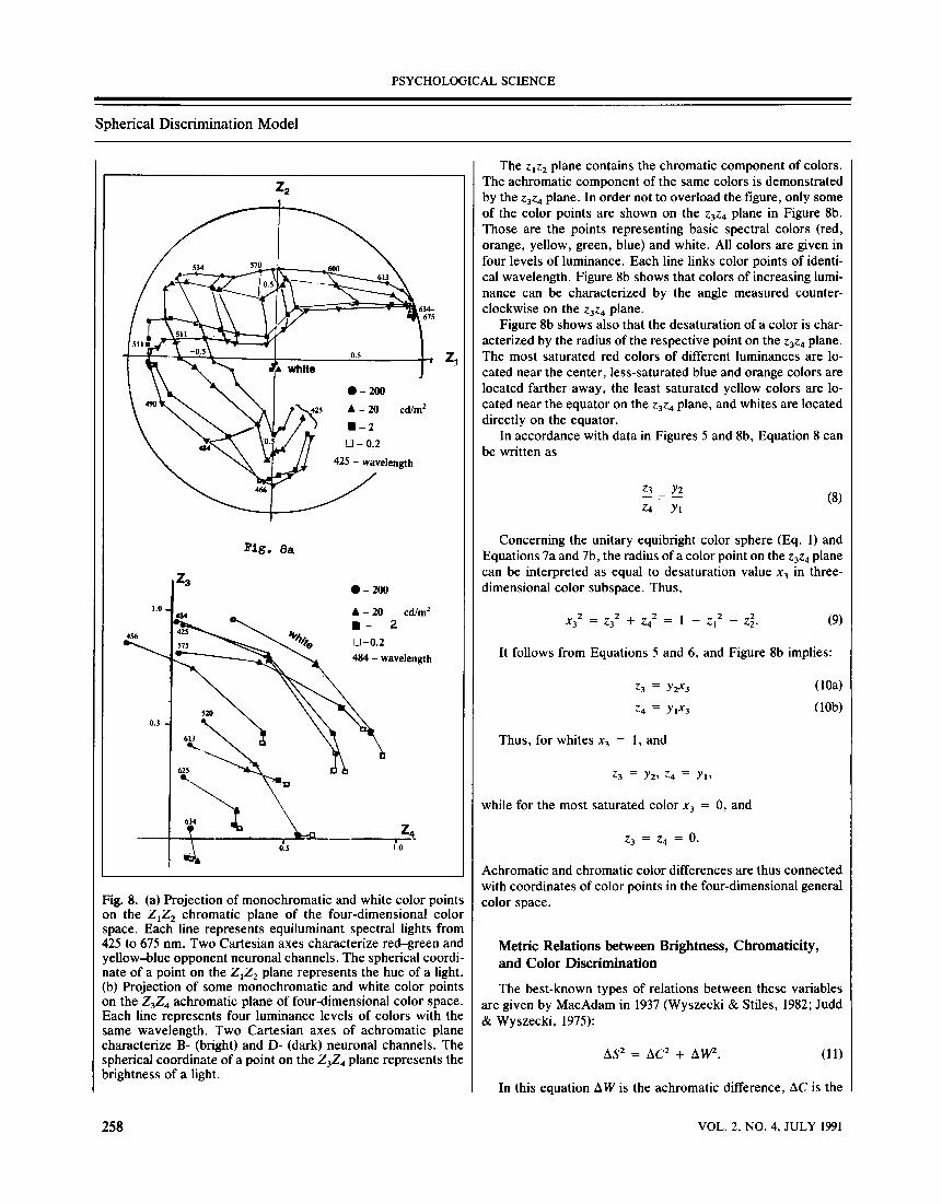
The configuration of 104 points can be projected on two coordinate planes, zxz2 and z3z4. Figure 8a shows a projection of monochromatic and white colors on the zxz2 plane on four luminance levels. Figure 8b gives the projections of the same points on the z3z4 plane.

DISCUSSION

Cartesian Coordinates of the Color Space Each color points' configuration in Figure 8a is evidently

related to a certain projection of equiluminant color points on the xxx2 plane of the three-dimensional color space (Fig. 2a). Differences between points representing colors of the sdme wavelength are in the range of the intensity-dependent Bezold- Brucke hue shift and the Purdy saturation shift. All spectral color points in each equiluminant configuration are located on the zxz2 plane according to their wavelength. The horizontal angle in this plane corresponds to color hue.

Comparing data in Figures 8a and 2a, we can derive

Zi = *i (7a)

and

z2 = x2. (7b)

VOL. 2, NO. 4, JULY 1991 257



Fig. 8. (a) Projection of monochromatic and white color points on the ZXZ2 chromatic plane of the four-dimensional color space. Each line represents equiluminant spectral lights from 425 to 675 nm. Two Cartesian axes characterize red-green and yellow-blue opponent neuronal channels. The spherical coordinate of a point on the ZXZ2 plane represents the hue of a light, (b) Projection of some monochromatic and white color points on the Z3Z4 achromatic plane of four-dimensional color space. Each line represents four luminance levels of colors with the same wavelength. Two Cartesian axes of achromatic plane characterize B- (bright) and D- (dark) neuronal channels. The spherical coordinate of a point on the Z3Z4 plane represents the brightness of a light.

The zxz2 plane contains the chromatic component of colors. The achromatic component of the same colors is demonstrated by the z3z4 plane. In order not to overload the figure, only some of the color points are shown on the z3z4 plane in Figure 8b. Those are the points representing basic spectral colors (red, orange, yellow, green, blue) and white. All colors are given in four levels of luminance. Each line links color points of identical wavelength. Figure 8b shows that colors of increasing luminance can be characterized by the angle measured counterclockwise on the z3z4 plane.

Figure 8b shows also that the desaturation of a color is characterized by the radius of the respective point on the z3z4 plane. The most saturated red colors of different luminances are located near the center, less-saturated blue and orange colors are located farther away, the least saturated yellow colors are located near the equator on the z3z4 plane, and whites are located directly on the equator.

In accordance with data in Figures 5 and 8b, Equation 8 can be written as

2 = * (8) za y\

Concerning the unitary equibright color sphere (Eq. 1) and Equations 7a and 7b, the radius of a color point on the z3z4 plane can be interpreted as equal to desaturation value jc3 in three- dimensional color subspace. Thus,

X32 = z32 + z42 = 1 - zx2 - zl (9)

It follows from Equations 5 and 6, and Figure 8b implies:

z3 = y2*3 (10a) z4 = yxx3 (10b)

Thus, for whites jc3 = 1, and

z3 = y2> z4 = yl9

while for the most saturated color x3 = 0, and

z3 = z4 = 0.

Achromatic and chromatic color differences are thus connected with coordinates of color points in the four-dimensional general color space.

Metric Relations between Brightness, Chromaticity, and Color Discrimination The best-known types of relations between these variables

are given by MacAdam in 1937 (Wyszecki & Stiles, 1982; Judd & Wyszecki, 1975):

AS2 = AC2 + AW2. (11)

In this equation AW is the achromatic difference, AC is the

258 VOL. 2, NO. 4, JULY 1991



chromatic difference, and AS is the total color difference between two lights. Another relation follows from the general four-dimensional spherical model of color discrimination (Eq. 6). Taking into account Equations 7a and 7b, Equation 3 can be rewritten as

AS2 = Ajc2 + Ajc2. + Azf + Az2.

In view of Equation 2,

AS2 + Ajc| = Ajc2 + Ax2. + Ajc| + Azf + &z24

and

AS2 = AC2 - Ajc2 + A3^Az2.

Equations 10a and 10b imply

AS2 = AC2 - Ajc2 + AU^)2 + AC*^,)2.

A is the difference between two colors i and j, consequently,

A(ry)2 = (xtfi - xjyjj)2, Axf = (xj3 - xj3)2;

thus, we obtain

AS2 = AC2 - Ax2 + (xi3yn - xj3yjl)2 + (xi3ya - Xj3yj2f.

It then follows that

AS2 = AC2 - 2x^x^x^11 - iynyjX + y^y^l

where (ynyji + y,-^) is the scalar product of the color vectors i and j on plane y\y2, consequently,

AS2 = AC2 + 2jcJ.3x/32sin2(a/2),

where a is the angle between vectors i andj, representing achromatic colors / and j respectively. According to Equation 5, 2sin(fl/2) on plane yxy2 is equal to brightness difference AW between color stimuli / and/ Hence,

AS2 = AC2 + 2xi3xj3AW2/2

or

AS2 = AC2 + xi3xj3AW2. (12)

Thus, there are three components in a total color difference. The first one is chromatic (AC), the second one is achromatic

(A WO, and the third one is a coefficient (jc3), connected with both chromatic and achromatic differences.

Comparing Equations 11 and 12, one can see that the first equation is a special case of the second one, for colors that differ only in the chromatic (xi3xj3 = 0) or achromatic (xl3xj3 = 1) components.

Acknowledgments - The authors gratefully acknowledge Prof. W. Estes for his creative editing, which improved the first version of our manuscript.

REFERENCES Boynton, R.M., & Gordon, J. (1965). Bezold-Bmcke hue shift measured by color-

naming technique. Journal of the Optical Society of America, 55, 78-86. De Valois, R.L (1973). Central mechanisms of color vision. In R. Jung (Ed.),

Handbook of sensory physiology, 7/3. Berlin: Springer. Gouras, P., & Zrenner, E. (1981). The color coding in the primate retina. Vision

Research, 21, 1591-1598. Hurvich, L.M., & Jameson, D. (1957). An opponent-process theory of color

vision. Psychological Review, 64, 384-404. Izmailov, Ch.A. (1980). Spherical model of color discrimination. Moscow: Mos-

cow State University (in Russian). Izmailov, Ch.A. (1982). Uniform color space and multidimensional scaling

(MDS). In H.G. Geissler & P. Petsold (Eds.), P sychophy sic al judgment and the process of perception (pp. 42-62). Berlin: VEB Deutsche Verlag der Wiss.

Izmailov, Ch.A., Sokolov, E.N., & Chernorizov, A.M. (1989). Psychophysiology of color vision. Moscow: Moscow State University (in Russian).

Judd, D.B. (1967). Interval scales, ratio scales, and additive for the sizes of differences perceived between members of geodesic series. Journal of the Optical Society of America, 57, 380-386.

Judd, D.B., & Wyszecki, G. (1975). Color in business, science, and industry. New York, London, Toronto, Sydney: John Wiley & Sons.

Jung, R. (1973). Visual perception and neurophysiology. In R. Jung (Ed.), Hand- book of sensory physiology, 7/3, part A. Berlin: Springer.

Mac Adam, D.L. (1963). Nonlinear relations of psychometric scale values to chromatic ity differences. Journal of the Optical Society of America, 53, 754.

Mac Adam, D.L. (1937). Projective transformations of I.C.I, color specifications. Journal of the Optical Society of America, 27, 194.

Poggio, G.F., Baker, F.N., Lamarre, Y., & Sanseverino, E.R. (1969). Afferent inhibition at input to visual cortex of the cat. Journal of the Optical Society of America, 32, 892-915.

Rabkin, B.E. (1971). Polychromatic plates. Moscow: Medicine (in Russian). Shepard, R.N., & Carroll, J.D. (1966). Parametric representation of nonlinear

data structures. In Krishnanian (Ed.), Multivariate analysis. New York: Academic Press.

Sokolov, E.N., & Izmailov, Ch.A. (1983). Conceptual reflex arc and color vision. In H.G. Geissler (Ed.), Modern issues in perception. Berlin: VEB Deutsche Verlag der Wiss., Amsterdam: North Holland.

Sokolov, E.N., & Izmailov, Ch.A. (1984). Color vision. Moscow: Moscow State University (in Russian).

Sokolov, E.N., Izmailov, Ch.A., & Schonebeck, B. (1982). Vergleichende Ex- perimente zur mehrdimensionalen Scalierung subjektiver Farbunterschiede und ihrer internen spharischen Representation. Zeitschrift fur Psychologie, 190, 275-293.

Wyszecki, G., & Stiles, W. (1982). Color science: Concepts and methods, qual- itative data and formulas. New York: Wiley.

Young, F.W., & Torgerson, W.S. (1967). Torsca, a Fortran 4 program for Shep- ard-Kruskal multidimensional scaling analysis. Behavioral Science, 12, (6).

Zrenner, E. (1983). Neurophysiological aspects of color vision in primates. Ber- lin, Heidelberg, New York: Springer Verlag.

(Received 11/26/90; Accepted 3/25/91)

VOL. 2, NO. 4, JULY 1991 259

Documents

PSYCHOLOGICAL SCIENCE Research Article · PSYCHOLOGICAL SCIENCE Research Article ... Apparatus A diagram of the ... optical lens' equipment of the apparatus, (b) Display of the test-surround