Embed Size (px)
Citation preview
Psychology 513Quantitative Models in Psychology
Class NotesSpring 2014
Robert M. McFatterUniversity of Louisiana
Lafayette
-2.5 -2
-1.5 -1
-0.5 0
0.5 1
1.5 2
2.5
-2.5
-1.25
0
1.252.5
2
2.5
3
3.5
4
4.5
5
5.5
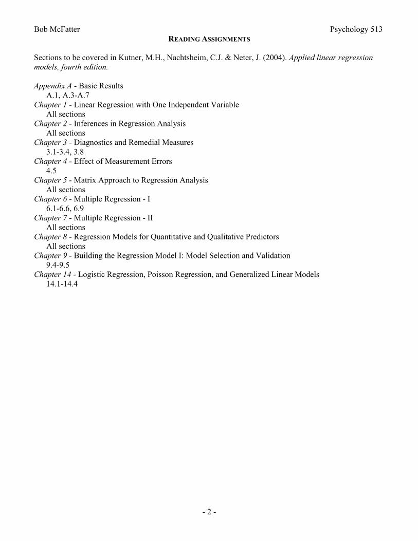
Positive Emotional Intensity
Extraversion
Neuroticism

Bob McFatter Psychology 513
- 2 -
Bob McFatter Psychology 513
- 1 -
SYLLABUS
Psychology 513 - Quantitative Models in PsychologyInstructor: Bob McFatterOffice: Girard Hall 222A; 482-6589Internet page: www.ucs.louisiana.edu/~rmm2440/E-mail: [email protected]
Texts: Kutner, M.H., Nachtsheim, C.J. & Neter, J. (2004). Applied linear regression models, fourth edition. New York: McGraw-Hill/Irwin OR Kutner, M.H., Neter, J., Nachtsheim, C.J. & Li, W. (2004). Applied linear statistical models, 5th international edition. New York: McGraw-Hill/Irwin.JMP Statistical Discovery Software, by SAS Institute. (available through UL site license at http://helpdesk.louisiana.edu)
Course Description
This course is designed to serve two main purposes. One objective is to provide an introduction to multiple correlation/regression and general linear models as basic analytical tools in psychological research. The other main objective is to familiarize students with a statistical package (JMP) available here and widely used throughout the country. Students should gain the practical skills necessary to enter, analyze, and interpret results for a variety of data sets using this package.
The first part of the course includes an introduction to the JMP statistical package mentioned above. Students use JMP to do familiar descriptive statistics, data screening, histograms, scatterplots, t-tests, etc.
A review of bivariate correlation and regression comes next if the backgrounds of the students require it. Topics covered include the relationship between correlation and regression, relevance of assumptions, effects of outliers, hypothesis testing, effects of measurement error and restricted variability, matrix formulation of regression analysis, the relation between dummy variable regression and t-test, and the interpretation of computer output including residual plots.
The remainder of the course is devoted to multiple regression and closely related topics. Consideration is given to the meaning and interpretation of regression weights, part and partial correlations, enhancer and suppressor effects, stepwise regression, multicollinearity problems, polynomial, interactive and nonlinear regression, logistic regression, analysis of covariance, and the relationship between regression and analysis of variance. Two exams, a midterm and a final, are given along with numerous homework assignments involving use of the computer to illustrate the theoretical aspects of the course.
Emergency Evacuation Procedures: A map of this floor is posted near the elevator marking the evacuation route and the Designated Rescue Areas. These are areas where emergency service personnel will go first to look for individuals who need assistance in exiting the building. Students who may need assistance should identify themselves to the teaching faculty.
Bob McFatter Psychology 513
- 2 -
READING ASSIGNMENTS
Sections to be covered in Kutner, M.H., Nachtsheim, C.J. & Neter, J. (2004). Applied linear regression models, fourth edition.
Appendix A - Basic ResultsA.1, A.3-A.7
Chapter 1 - Linear Regression with One Independent VariableAll sections
Chapter 2 - Inferences in Regression AnalysisAll sections
Chapter 3 - Diagnostics and Remedial Measures3.1-3.4, 3.8
Chapter 4 - Effect of Measurement Errors4.5
Chapter 5 - Matrix Approach to Regression AnalysisAll sections
Chapter 6 - Multiple Regression - I6.1-6.6, 6.9
Chapter 7 - Multiple Regression - IIAll sections
Chapter 8 - Regression Models for Quantitative and Qualitative PredictorsAll sections
Chapter 9 - Building the Regression Model I: Model Selection and Validation9.4-9.5
Chapter 14 - Logistic Regression, Poisson Regression, and Generalized Linear Models14.1-14.4
Bob McFatter Psychology 513
- 3 -
513 NOTES OUTLINE
A concise and useful review of basic statistical ideas is given in Kutner et al.’s Appendix A, sections A.1, A.3-A.7.
The model underlying general linear model (of which regression analysis and ANOVA are special cases) follows the general form: Data = Fit + Residual. One way this idea can be applied to the linear regression case is to describe each individual's score in the data set as being composed of 2 pieces: the
predicted Y from some model, Y , and a residual or error component, e.
Y Y e [1]
It follows that e Y Y and reflects how far away the actual Y score is from the predicted Y score. The idea here is to hypothesize a model of the data and find estimates of the parameters of the model that make it fit the data as well as possible (i.e., minimize in some way the size of the residuals). The most common method is to find estimates of the parameters that make the sum of the squared residuals in the sample as small as possible. This is called ‘least squares’ estimation.
The model we focus on first is the linear regression model. The simplest case of linear regression analysis is the bivariate case: one predictor variable, X, and one criterion variable, Y. This involves fitting the sample data with a straight line of the form
Y b b X 0 1 [2]
where b0 is the Y-intercept, and b1 is the slope in the sample (these values being estimates of the population parameters 0 and 1).
The least squares estimators, b0 and b1, can be shown to be as follows:
b r
s
s
XYX Y
n
XX
n
Y
X1
2
2
and [3]
b M b MY X0 1 [4]
Here r is the correlation between X and Y, sY and sX are the standard deviations of Y and X, respectively, and MY and MX are the means of Y and X, respectively.
Example. Consider the following small data set.X Y6 16 23 33 42 5
The raw calculations may be done with X Y XY X 20 15 49 942, , , and
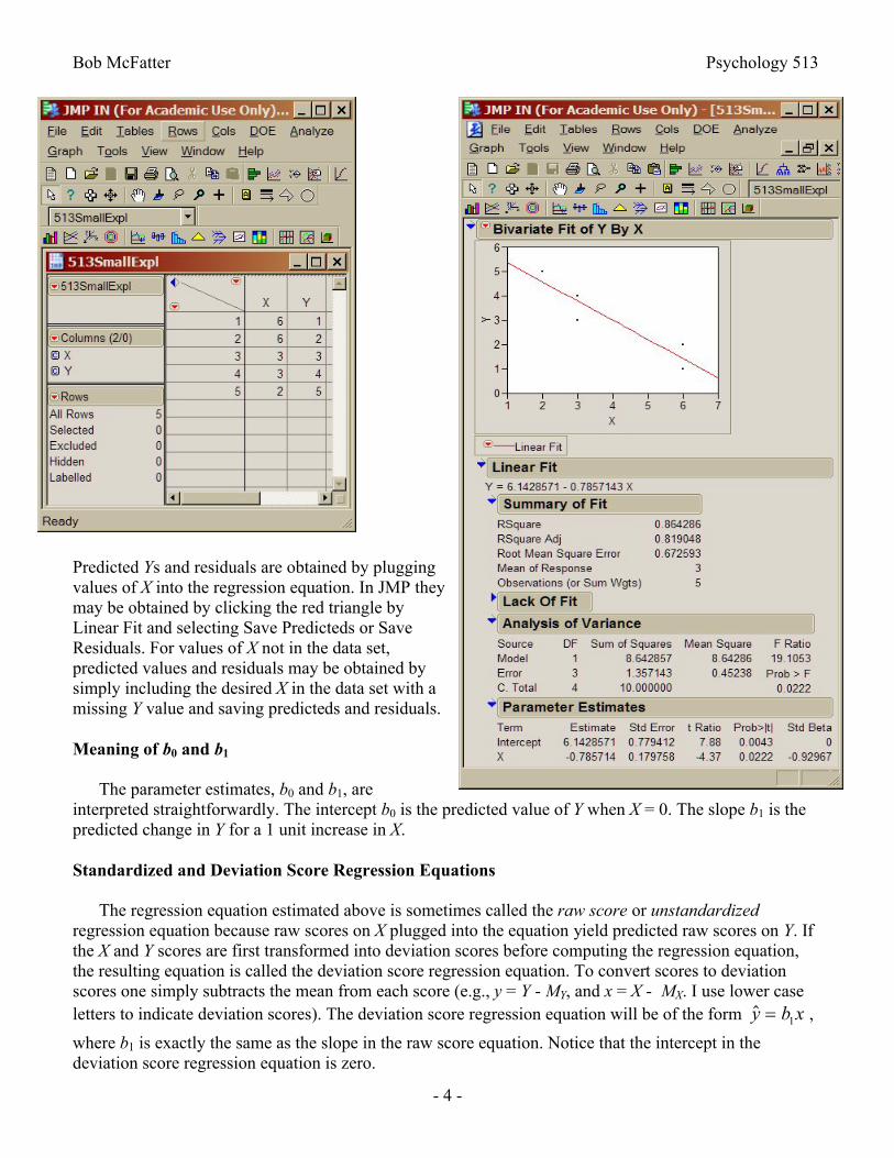
MX = 4 and MY = 3, leading to . .Y X 61428571 0 7857143One way to do the JMP analysis using the Fit Y By X platform is as follows:
Bob McFatter Psychology 513
- 4 -
Predicted Ys and residuals are obtained by plugging values of X into the regression equation. In JMP they may be obtained by clicking the red triangle by Linear Fit and selecting Save Predicteds or Save Residuals. For values of X not in the data set, predicted values and residuals may be obtained by simply including the desired X in the data set with a missing Y value and saving predicteds and residuals.
Meaning of b0 and b1
The parameter estimates, b0 and b1, are interpreted straightforwardly. The intercept b0 is the predicted value of Y when X = 0. The slope b1 is the predicted change in Y for a 1 unit increase in X.
Standardized and Deviation Score Regression Equations
The regression equation estimated above is sometimes called the raw score or unstandardizedregression equation because raw scores on X plugged into the equation yield predicted raw scores on Y. If the X and Y scores are first transformed into deviation scores before computing the regression equation, the resulting equation is called the deviation score regression equation. To convert scores to deviation scores one simply subtracts the mean from each score (e.g., y = Y - MY, and x = X - MX. I use lower case letters to indicate deviation scores). The deviation score regression equation will be of the form y b x 1 ,
where b1 is exactly the same as the slope in the raw score equation. Notice that the intercept in the deviation score regression equation is zero.
Bob McFatter Psychology 513
- 5 -
It is actually more common to transform the X and Y scores to standardized (Z) scores than to deviation scores. When this is done, the resulting equation is called the standardized regression equation.
The form of the standardized regression equation is Z rZY X . Notice that the intercept of the
standardized regression equation is zero and the slope is r, the correlation coefficient between X and Y. This equation can be obtained in JMP by right-clicking in the Parameter Estimates table and selecting Columns|Std Beta. It is, unfortunately, common practice to refer to standardized regression coefficients (or weights or slopes; they all mean the same thing) as ‘standardized betas’ even though the coefficients are not population parameters.
One interpretation of the correlation coefficient r, then, is as the slope of the standardized regression equation. Thus, an r of .6 would mean that a 1 standard deviation increase in the value of X would lead us to predict a .6 standard deviation increase in the value of Y.
The predictions made are the same regardless of which form (raw score, deviation score, standard score) of the regression equation is used.
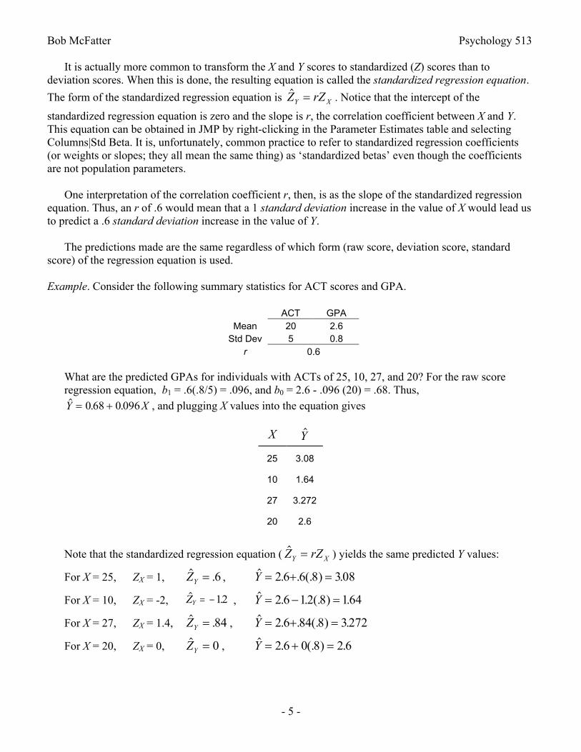
Example. Consider the following summary statistics for ACT scores and GPA.
ACT GPAMean 20 2.6
Std Dev 5 0.8r 0.6
What are the predicted GPAs for individuals with ACTs of 25, 10, 27, and 20? For the raw score regression equation, b1 = .6(.8/5) = .096, and b0 = 2.6 - .096 (20) = .68. Thus, . .Y X 0 68 0 096 , and plugging X values into the equation gives
X Y
25 3.08
10 1.64
27 3.272
20 2.6
Note that the standardized regression equation ( Z rZY X ) yields the same predicted Y values:
For X = 25, ZX = 1, .ZY 6 , . . (. ) .Y 2 6 6 8 308
For X = 10, ZX = -2, .ZY 12 , . . (. ) .Y 2 6 12 8 164
For X = 27, ZX = 1.4, .ZY 84 , . . (. ) .Y 2 6 84 8 3272
For X = 20, ZX = 0, ZY 0 , . (. ) .Y 2 6 0 8 2 6
Bob McFatter Psychology 513
- 6 -
One interesting and important phenomenon implied by the standardized regression equation is called regression toward the mean. Because it is always the case that 0 ≤ |r| ≤ 1, the predicted value of ZY will be ≤ in absolute value than ZX, that is, generally closer to the mean of zero (in standard deviation units) than ZX.
Assumptions
Certain assumptions are commonly made to aid in drawing inferences in regression analysis. Those assumptions may be stated as follows:
1) The means of all the conditional distributions of Y|X lie on a straight line (linearity).2) The variances of the conditional distributions of Y|X are all equal (homoscedasticity).3) The conditional distributions of Y|X are all normal.4) The points in the sample are a random sample from the population of points.If homoscedasticity holds, then the population variance of any conditional distribution of Y|X is equal
to the variance of the population of residuals, and an estimate of that variance may be used as an estimate of the variance of Ys for any given X. The most commonly used estimate of the variance of the residuals is the mean square error (MSE) where MSE = Σ e2/(n - 2) = SSE/dfE. The square root of this quantity (or Root MSE) is sometimes called the standard error of estimate for the regression analysis and would, of course, be an estimate of the standard deviation of each of the conditional distributions of Y|X. It can be thought of as how far off typically one would expect actual Y values to be from the predicted Y of the regression equation.
ANOVA Partitioning
It is common to construct an ANOVA partitioning of the variation (SS) of the Y scores in a regression analysis.
The total variation of the raw Y scores is measured by SSY or SSTO = ( )Y M yY 2 2 .
The variation of the predicted Y scores is SSR = ( ) Y M yY 2 2 .
The variation of the residuals is SSE = ( )Y Y e 2 2
It is straightforward to show that SSTO = SSR + SSE. This is another example of the Data = Fit + Residual idea. The total variation of the Y scores can be broken down into two pieces: (1) predictable variation due to the model (SSR); and (2) unpredictable, noise, or error variation (SSE). It also turns out that the proportion of variation in Y that is predictable is equal to r2:
r rSSR
SSTOXY YY
2 2 . [5]
Sums of squares (SS) are converted into sample variance estimates or mean squares (MS) by dividing by the appropriate df. For the ANOVA breakdown here, dfTO = n - 1, dfR = 1, and dfE = n - 2, so that MSTO = SSTO/dfTO, MSR = SSR/dfR, and MSE = SSE/dfE.
MSTO would thus be simply the sample variance of the Y scores, and MSE would be the sample variance of the residuals using n - 2 as the df.
The overall F-ratio from the ANOVA breakdown, F(dfR, dfE) = MSR/MSE, tests the null hypothesis that none of the variation in Y is linearly predictable from X. In the bivariate case this is exactly equivalent to the null hypothesis that the population slope, β1, is equal to zero.
Bob McFatter Psychology 513
- 7 -
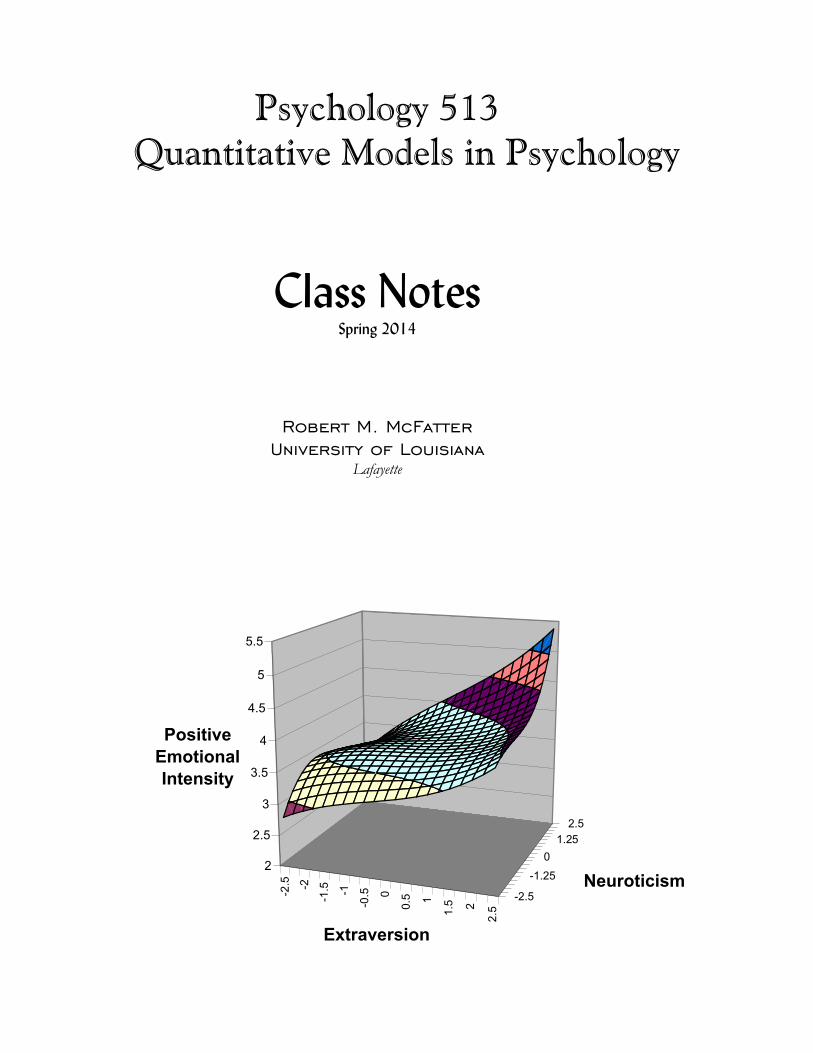
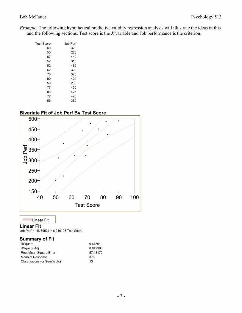
Example. The following hypothetical predictive validity regression analysis will illustrate the ideas in this and the following sections. Test score is the X variable and Job performance is the criterion.
Test Score Job Perf69 32055 22367 44052 31082 48562 32070 37090 49050 20077 45083 42572 47555 380
Bivariate Fit of Job Perf By Test Score
150
200
250
300
350
400
450
500
Job
Per
f
40 50 60 70 80 90 100
Test Score
Linear Fit
Linear FitJob Perf = -46.69521 + 6.216106 Test Score
Summary of FitRSquare 0.67861RSquare Adj 0.649393Root Mean Square Error 57.13172Mean of Response 376Observations (or Sum Wgts) 13

Bob McFatter Psychology 513
- 8 -
Analysis of Variance
Source DF Sum of Squares Mean Square F RatioModel 1 75811.63 75811.6 23.2264Error 11 35904.37 3264.0 Prob > FC. Total 12 111716.00 0.0005
Parameter EstimatesTerm Estimate Std Error t Ratio Prob>|t| Lower 95% Upper 95% Std BetaIntercept -46.69521 89.12735 -0.52 0.6107 -242.8632 149.47277 0Test Score 6.216106 1.289816 4.82 0.0005 3.3772398 9.0549723 0.823778
Test Score Job Perf Pred Formula Job Perf
Residual Job Perf PredSE Job Perf
StdErr Indiv Job Perf Studentized Resid Job Perf
69 320 382.216106 -62.216106 15.8978975 59.3024188 -1.13377455 223 295.190622 -72.190622 23.0701597 61.6138459 -1.381198967 440 369.783894 70.216106 15.8978975 59.3024188 1.2795592752 310 276.542304 33.4576962 26.0186032 62.777396 0.6577975982 485 463.025484 21.9745158 24.0239498 61.9772853 0.4239307262 320 338.703364 -18.703364 17.6343428 59.7913353 -0.344178270 370 388.432212 -18.432212 16.0540967 59.3444838 -0.336171890 490 512.754332 -22.754332 32.5003751 65.7290508 -0.484270750 200 264.110092 -64.110092 28.1086155 63.6720346 -1.288937577 450 431.944954 18.0550459 19.6426374 60.4141286 0.3365410783 425 469.24159 -44.24159 25.007905 62.3652872 -0.861272972 475 400.864424 74.1355759 16.6642591 59.5124463 1.3566171955 380 295.190622 84.8093782 23.0701597 61.6138459 1.622629360 . 326.271152 . 18.909034 60.1796087 .
Sampling Distributions of b0 and b1
Because b0 and b1 are sample statistics, their values will fluctuate from sample to sample from the same population of X and Y values. It is common to assume a model to describe the population of X and Yvalues, and consider b0 and b1 to be estimates of the parameters of the model. The most commonly assumed model is the normal error regression model:
Yi = β0 + β 1 Xi + εi [6]where:
Yi is the observed value of the criterion variable for the ith observationXi is a known constant, the value of the predictor variable for the ith observationβ 0 and β 1 are parametersthe residuals, εi, are independent and N(0, σ2) [i.e., normally distributed with mean 0 and variance
σ2]i = 1, ..., n
Thus, b0 and b1 are estimates of β0 and β1, and will, like all statistics, have sampling distributions associated with them. Under the normal error regression model above, the sampling distributions of b0 and b1 will both be normal. The means of the sampling distributions will be E{b0} = β0 and E{b1} = β1, respectively. Thus, b0 and b1 are both unbiased estimators of their respective population parameters.
The variances of the two sampling distributions may be shown to be:
For b0: 20
22
2
1{ }
( )b
n
M
X MX
i X
. [7]
Bob McFatter Psychology 513
- 9 -
For b1:
21
2
2{ }
( )b
X Mi X
. [8]
Sample estimates of these variances may be obtained by replacing σ2 with its sample estimate, the mean square error (MSE). Thus,
s b MSEn
M
X MX
i X
20
2
2
1{ }
( )
and [9]
s bMSE
X Mi X
21 2
{ }( )
. [10]
The square roots of these quantities are called the standard errors of the parameter estimates and are given by most regression programs (including JMP) in a column next to the estimates themselves.The standard errors of b0 and b1 reflect how far off, typically, one would expect the sample values, b0 and b1, to be from β0 and β1, respectively. The standard errors of b0 and b1 can be used to construct confidence intervals around b0 and b1 and to conduct hypothesis tests about β0 and β1. To avoid the somewhat cumbersome curly brace notation, I will generally use sb0 and sb1 to refer to the standard errors of b0 and b1.
In the predictive validity example above, sb0 = 89.12735 and sb1 =1.289816.
Hypothesis Tests and Confidence Intervals for β1, β0, and ρ
It is common to test hypotheses and construct confidence intervals for β1, β0 and ρ where ρ is the population correlation between X and Y. Because
1
Y
X
, [11]
it is clear that β1 = 0 when ρ = 0, and vice versa. Therefore, testing the null hypothesis that either of these is equal to zero is exactly equivalent to testing the hypothesis that the other is zero. These equivalent hypotheses are the most commonly tested null hypotheses in bivariate regression analyses because they test whether there is a relation between X and Y, often the hypothesis of most interest in the analysis.
When the sampling distribution of a statistic is normal, and the standard deviation of the sampling distribution of that statistic (i.e., the standard error of the statistic) can be estimated, a t-test may beconstructed to test null hypotheses about the value of the population parameter the statistic estimates. The general form of the t-test is
tStatistic Hypothesized value
Estimated Std Error of the Statistic
. [12]
Thus, to test H0: β 1 = 0, the appropriate t-test is
tb
s
b
sb b
1 10
1 1
.
Bob McFatter Psychology 513
- 10 -
In the example above, t(11) = 6.216106/1.289816 = 4.82, p = .0005, and the H0: β1 = 0, would be rejected even at α = .001.
The estimated standard error of r when ρ = 0 is sr
nr
1
2
2
, so testing the H0: ρ = 0 can be carried out
with tr
s
r n
rr
2
1 2. The df associated with the t-tests for these two null hypotheses are n - 2.
Because the two t-tests are testing equivalent null hypotheses, the values of t obtained in the two tests will be exactly the same. It is also important to note that the overall F-ratio from the bivariate regression analysis described above, F(dfR, dfE) = F(1, n - 2)= MSR/MSE, is exactly equivalent to the square of the tvalue obtained testing the null hypotheses β1 = 0 or ρ = 0. So, these three hypothesis tests all test the same basic question and will all have exactly the same p-level.
In the example above, r = 0.823778, and plugging this value into the equation above yields t(11) = 4.82, p = .0005. Also, F(1, 11) = 23.23, p = .0005. Note that 23.23 = 4.822.
Similar logic yields a test of H0: β0 = 0 of the form tb
sb
0
0
, but this hypothesis is usually not of as
much interest as the ones described above. JMP provides values for all the crucial components of these hypothesis tests including t values, F-ratio, and p-levels.
In addition, confidence intervals around b0 and b1 may be obtained in the usual way. For example, the 1 - α confidence limits for β 1 would be b1 ± t(1 - α/2, n - 2) sb1. In JMP the 95% confidence limits for β0
and β1 may be obtained by right-clicking on the Parameter Estimates table and selecting Columns|Lower 95% and Upper 95%.
In the example above, the 95% confidence interval for β1 would be (from the output): (3.38, 9.05).
Confidence intervals around r may be obtained using the Fisher’s Zr transformation:
Zr = tanh-1(r) = 1
2
1
1ln
r
r. Fisher’s Zr values are approximately normally distributed with a standard
deviation of Zr n
1
3. Ordinary normal distribution methods can thus be used to find confidence
intervals around the Zr values. The ends of the confidence interval obtained may then be transformed back to r values using r = tanh( Zr ). [See p. 85-86 in Kutner et al. or an introductory statistics text such as HyperStat Online (http://davidmlane.com/hyperstat/) for more details and examples.]
Two Kinds of Prediction (E{Y|X} and Y|X) [See p. 52 and 55 in Kutner et al.]
There are two kinds of prediction that one might consider following a regression analysis:1) prediction of the mean value of Y for all observations with a given X score (i.e., E{Y|X});2) prediction of the value of Y for an individual observation with a given X score (i.e., Y|X).
It is important to recognize that the predicted value of Y will be the same for both cases, namely, Y . However, the uncertainty associated with the two kinds of prediction will differ.
Bob McFatter Psychology 513
- 11 -
In the first case we are trying to predict the Y value of the population regression line for the given X, and the uncertainty associated with that prediction will be simply how far typically we would expect sample regression lines to ‘wobble’ in the Y direction around the population regression line.
In the second case we must consider not only this wobble of sample regression lines around the population regression line, but also the variability of individual Ys around the sample regression line. Thus, the variability in the second case will simply be the variability in the first case (i.e., wobble) plus an additional component reflecting the variability of the Ys around the sample regression line.
Kutner et al. show that a sample estimate of the (wobble) variance of the Y s around the population regression line is
s Y MSEn
X M
X Mh
h X
i X
2
2
2
1
, [13]
where Xh is the value of X for which we wish to estimate the mean Y value (i.e., Yh ). Notice that the
uncertainty depends on how far away Xh is away from the mean of X, MX. The further Xh is from MX, the greater the uncertainty. The square root of this quantity is called the ‘Std Error of Predicted’ by JMP and can be obtained for each observation from the Fit Model platform after a regression analysis has been performed by right-clicking on a section title and selecting Save Columns|Std Error of Predicted. In the above example, the predicted job performance for individuals with a test score of 60 is 326.27. One would expect this value to be off typically by 18.91 points from the true mean performance of individuals with a score of 60 on the test.
A sample estimate of the variance of the individual Ys around the sample regression line would then be the sum of the ‘wobble’ variance above and the MSE. Kutner et al. call this s2{pred}:
s pred MSEn
X M
X Mh X
i X
2
2
211
. [14]
The square root of this quantity is called ‘Std Error of Individual’ by JMP and can be obtained for each observation by selecting Save Columns|Std Error of Individual. In the above example, the predicted job performance for an individual with a test score of 60 is 326.27. One would expect this value to be off typically by 60.18 points from the actual performance of an individual with a score of 60 on the test. It is instructive to compare this interpretation with the interpretation at the end of the last paragraph.
The standard errors of predicted and individual scores may be used with the t distribution in the usual way to construct confidence intervals for the two kinds of prediction. In the Fit Y by X platform of JMP, plots of the 95% confidence intervals for the two kinds of prediction may be obtained by clicking the Linear Fit red triangle and selecting ‘Confid Curves Fit’ and ‘Confid Curves Individual,’ respectively. (See the figure in the output for the example above.) Actual upper and lower bounds of the 95% confidence intervals for each observation may be obtained from the Fit Model platform regression analysis by right-clicking on a section title and selecting Save Columns|Mean Confidence Interval or Indiv Confidence Interval, respectively.
Residuals Analysis and Outliers
Examining the residuals, ei, from a regression analysis is often helpful in detecting violations of the assumptions underlying the model. The least squares estimation procedure forces the residuals to sum to
Bob McFatter Psychology 513
- 12 -
zero and to have a zero correlation with the predictor variable X. However, important diagnostic information can often be gained by analyzing the obtained residuals in various ways. It is common, for
example, to plot the residuals as a function of X or Y (the two plots would look exactly the same except
for the scale of the horizontal axis–make sure you see why). This kind of plot can easily reveal nonlinearity of the relation or violations of the homoscedasticity assumption. For example, the following scatterplot and residual plot illustrates violations of both the linearity and homoscedasticity assumptions.
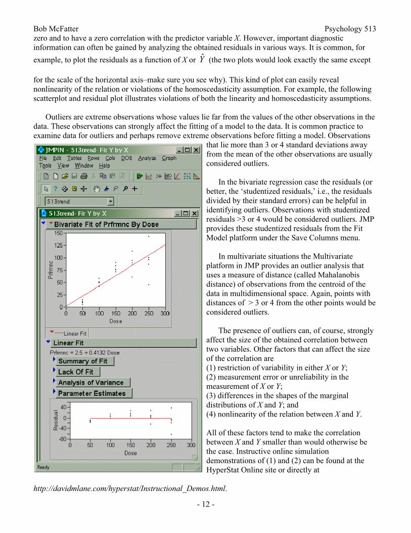
Outliers are extreme observations whose values lie far from the values of the other observations in the data. These observations can strongly affect the fitting of a model to the data. It is common practice to examine data for outliers and perhaps remove extreme observations before fitting a model. Observations
that lie more than 3 or 4 standard deviations away from the mean of the other observations are usually considered outliers.
In the bivariate regression case the residuals (or better, the ‘studentized residuals,’ i.e., the residuals divided by their standard errors) can be helpful in identifying outliers. Observations with studentized residuals >3 or 4 would be considered outliers. JMPprovides these studentized residuals from the Fit Model platform under the Save Columns menu.
In multivariate situations the Multivariate platform in JMP provides an outlier analysis that uses a measure of distance (called Mahalanobis distance) of observations from the centroid of the data in multidimensional space. Again, points with distances of > 3 or 4 from the other points would be considered outliers.
The presence of outliers can, of course, strongly affect the size of the obtained correlation between two variables. Other factors that can affect the size of the correlation are (1) restriction of variability in either X or Y;(2) measurement error or unreliability in the measurement of X or Y;(3) differences in the shapes of the marginal distributions of X and Y; and(4) nonlinearity of the relation between X and Y.
All of these factors tend to make the correlation between X and Y smaller than would otherwise be the case. Instructive online simulation demonstrations of (1) and (2) can be found at the HyperStat Online site or directly at
http://davidmlane.com/hyperstat/Instructional_Demos.html.

Bob McFatter Psychology 513
- 13 -
Two-Predictor Models
When there are two predictors in the model the simplest fitted regression equation becomesY b b X b X 0 1 1 2 2 . [15]
As we have seen, the simple bivariate regression equation (Equation [2]) represents the finding of the best fitting straight line to a two dimensional scatterplot of X and Y. When there are two predictors in the model, the equation in [15] represents the finding of the best fitting plane to a three dimensional cloud of points in 3-space. The ‘Fit’ part of Data = Fit + Residual is now a plane rather than a straight line. By adding predictors to, or changing the functional form of predictors in, equation [15] we may generate a huge variety of models of data, but the basic principles of model fitting, estimation of parameters, and hypothesis testing remain the same.
The sample statistics b0, b1, and b2 in [15] are estimates of the population parameters β0, β1, and β2. Formulas for the least squares estimates of the population parameters β1 and β2 may be found and involve the sample variances and covariances of the Xs and Y. These formulas quickly become very complex with more than two predictors, and it is generally most satisfactory to solve the least squares estimation problem in matrix form. We will consider that later. It is impractical to compute these estimates with a calculator, so we generally use a statistics program. The intercept b0, however, will always be b0 = MY - b1M1 - b2M2 . . . regardless of the number of predictors, where MY is the mean of Y, M1 the mean of X1, etc.
Example.The following example with hypothetical data from a study using IQ and Extraversion scores to
predict Sale Success will illustrate the analysis. Here is the JMP output from the Fit Model platform.Raw DataIQ Extr Success98 38 495 33 3104 47 5108 43 577 41 5115 44 4103 50 6108 46 6109 46 4100 39 5
Variable N Mean Std Dev Min MaxExtr 10 42.7 5.03432661 33 50IQ 10 101.7 10.4780193 77 115Success 10 4.7 0.9486833 3 6
Multivariate Correlations
IQ Extr SuccessIQ 1.0000 0.4510 0.0458Extr 0.4510 1.0000 0.7003Success 0.0458 0.7003 1.0000

Bob McFatter Psychology 513
- 14 -
MODEL 1 - IQ ALONE
Response SuccessSummary of FitRSquare 0.0021RSquare Adj -0.12264Root Mean Square Error 1.005173Mean of Response 4.7Observations (or Sum Wgts) 10
Analysis of VarianceSource DF Sum of Squares Mean Square F RatioModel 1 0.0170124 0.01701 0.0168Error 8 8.0829876 1.01037 Prob > FC. Total 9 8.1000000 0.9000
Parameter EstimatesTerm Estimate Std Error t Ratio Prob>|t| Std BetaIntercept 4.2780083 3.267579 1.31 0.2268 0IQ 0.0041494 0.031977 0.13 0.9000 0.045829
Effect TestsSource Nparm DF Sum of Squares F Ratio Prob > FIQ 1 1 0.01701245 0.0168 0.9000
Sequential (Type 1) TestsSource Nparm DF Seq SS F Ratio Prob > FIQ 1 1 0.01701245 0.0168 0.9000
MODEL 2 - EXTR ALONE
Response SuccessSummary of FitRSquare 0.490369RSquare Adj 0.426665Root Mean Square Error 0.718333Mean of Response 4.7Observations (or Sum Wgts) 10
Analysis of VarianceSource DF Sum of Squares Mean Square F RatioModel 1 3.9719860 3.97199 7.6976Error 8 4.1280140 0.51600 Prob > FC. Total 9 8.1000000 0.0241
Parameter EstimatesTerm Estimate Std Error t Ratio Prob>|t| Std BetaIntercept -0.934678 2.043575 -0.46 0.6596 0Extr 0.1319597 0.047562 2.77 0.0241 0.700263
Effect TestsSource Nparm DF Sum of Squares F Ratio Prob > FExtr 1 1 3.9719860 7.6976 0.0241
Sequential (Type 1) TestsSource Nparm DF Seq SS F Ratio Prob > FExtr 1 1 3.9719860 7.6976 0.0241
Bob McFatter Psychology 513
- 15 -
MODEL 3 - IQ FIRST
Response SuccessSummary of FitRSquare 0.581862RSquare Adj 0.462394Root Mean Square Error 0.69559Mean of Response 4.7Observations (or Sum Wgts) 10
Analysis of VarianceSource DF Sum of Squares Mean Square F RatioModel 2 4.7130814 2.35654 4.8704Error 7 3.3869186 0.48385 Prob > FC. Total 9 8.1000000 0.0473
Parameter EstimatesTerm Estimate Std Error t Ratio Prob>|t| Std BetaIntercept 0.9560894 2.499998 0.38 0.7135 0IQ -0.030684 0.024793 -1.24 0.2558 -0.3389Extr 0.1607603 0.051602 3.12 0.0170 0.853098
Effect TestsSource Nparm DF Sum of Squares F Ratio Prob > FIQ 1 1 0.7410954 1.5317 0.2558Extr 1 1 4.6960689 9.7057 0.0170
Sequential (Type 1) TestsSource Nparm DF Seq SS F Ratio Prob > FIQ 1 1 0.0170124 0.0352 0.8566Extr 1 1 4.6960689 9.7057 0.0170
MODEL 4 - EXTR FIRST
Response SuccessSummary of FitRSquare 0.581862RSquare Adj 0.462394Root Mean Square Error 0.69559Mean of Response 4.7Observations (or Sum Wgts) 10
Analysis of VarianceSource DF Sum of Squares Mean Square F RatioModel 2 4.7130814 2.35654 4.8704Error 7 3.3869186 0.48385 Prob > FC. Total 9 8.1000000 0.0473
Parameter EstimatesTerm Estimate Std Error t Ratio Prob>|t| Std BetaIntercept 0.9560894 2.499998 0.38 0.7135 0Extr 0.1607603 0.051602 3.12 0.0170 0.853098IQ -0.030684 0.024793 -1.24 0.2558 -0.3389
Effect TestsSource Nparm DF Sum of Squares F Ratio Prob > FExtr 1 1 4.6960689 9.7057 0.0170IQ 1 1 0.7410954 1.5317 0.2558
Sequential (Type 1) TestsSource Nparm DF Seq SS F Ratio Prob > FExtr 1 1 3.9719860 8.2092 0.0242IQ 1 1 0.7410954 1.5317 0.2558
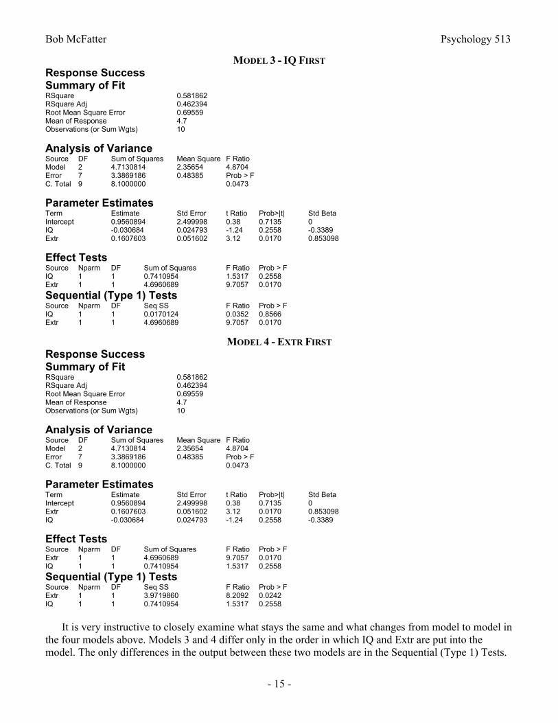
It is very instructive to closely examine what stays the same and what changes from model to model in the four models above. Models 3 and 4 differ only in the order in which IQ and Extr are put into the model. The only differences in the output between these two models are in the Sequential (Type 1) Tests.
Bob McFatter Psychology 513
- 16 -
Interpretation of the Parameter Estimates
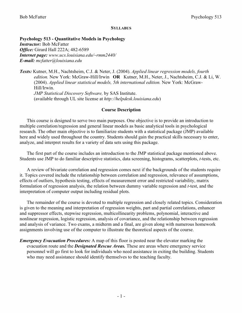
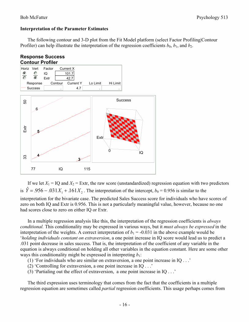
The following contour and 3-D plot from the Fit Model platform (select Factor Profiling|Contour Profiler) can help illustrate the interpretation of the regression coefficients b0, b1, and b2.
Response SuccessContour ProfilerHoriz Vert
IQExtr
Factor
101.7 42.7
Current X
Success
Response
.
Contour
4.7
Current Y
.
Lo Limit
.
Hi Limit
50E
xtr
33
4
5
34
5
34
5
6
3
77 IQ 115
0 IQ
Extr
Success
If we let X1 = IQ and X2 = Extr, the raw score (unstandardized) regression equation with two predictors
is . . .Y X X 956 031 1611 2 . The interpretation of the intercept, b0 = 0.956 is similar to the
interpretation for the bivariate case. The predicted Sales Success score for individuals who have scores of zero on both IQ and Extr is 0.956. This is not a particularly meaningful value, however, because no one had scores close to zero on either IQ or Extr.
In a multiple regression analysis like this, the interpretation of the regression coefficients is always conditional. This conditionality may be expressed in various ways, but it must always be expressed in the interpretation of the weights. A correct interpretation of b1 = -0.031 in the above example would be ‘holding individuals constant on extraversion, a one point increase in IQ score would lead us to predict a .031 point decrease in sales success. That is, the interpretation of the coefficient of any variable in the equation is always conditional on holding all other variables in the equation constant. Here are some other ways this conditionality might be expressed in interpreting b1:
(1) ‘For individuals who are similar on extraversion, a one point increase in IQ . . .’(2) ‘Controlling for extraversion, a one point increase in IQ . . .’(3) ‘Partialing out the effect of extraversion, a one point increase in IQ . . .’
The third expression uses terminology that comes from the fact that the coefficients in a multiple regression equation are sometimes called partial regression coefficients. This usage perhaps comes from
Bob McFatter Psychology 513
- 17 -
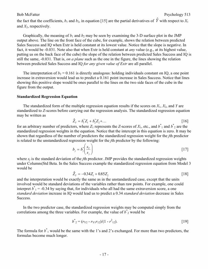
the fact that the coefficients, b1 and b2, in equation [15] are the partial derivatives of Y with respect to X1
and X2, respectively.
Graphically, the meaning of b1 and b2 may be seen by examining the 3-D surface plot in the JMP output above. The line on the front face of the cube, for example, shows the relation between predicted Sales Success and IQ when Extr is held constant at its lowest value. Notice that the slope is negative. In fact, it would be -0.031. Note also that when Extr is held constant at any value (e.g., at its highest value, putting us on the back face of the cube) the slope of the relation between predicted Sales Success and IQ is still the same, -0.031. That is, on a plane such as the one in the figure, the lines showing the relation between predicted Sales Success and IQ for any given value of Extr are all parallel.
The interpretation of b2 = 0.161 is directly analogous: holding individuals constant on IQ, a one point increase in extraversion would lead us to predict a 0.161 point increase in Sales Success. Notice that lines showing this positive slope would be ones parallel to the lines on the two side faces of the cube in the figure from the output.
Standardized Regression Equation
The standardized form of the multiple regression equation results if the scores on X1, X2, and Y are standardized to Z-scores before carrying out the regression analysis. The standardized regression equation may be written as
* *Z b Z b ZY 1 1 2 2 [16]for an arbitrary number of predictors, where Z1 represents the Z-scores of X1, etc., and b*
1 and b*2 are the
standardized regression weights in the equation. Notice that the intercept in this equation is zero. It may be shown that regardless of the number of predictors the standardized regression weight for the jth predictor is related to the unstandardized regression weight for the jth predictor by the following:
b bs
sj jY
j
* [17]
where sj is the standard deviation of the jth predictor. JMP provides the standardized regression weights under Columns|Std Beta. In the Sales Success example the standardized regression equation from Model 3 would be
. .Z Z ZY 0 34 0 851 2 [18]and the interpretation would be exactly the same as in the unstandardized case, except that the units involved would be standard deviations of the variables rather than raw points. For example, one could interpret b*
1 = -0.34 by saying that, for individuals who all had the same extraversion score, a one standard deviation increase in IQ would lead us to predict a 0.34 standard deviation decrease in Sales Success.
In the two predictor case, the standardized regression weights may be computed simply from the correlations among the three variables. For example, the value of b*
2 would be
b*2 = (rY2 - rY1r12)/(1 - r2
12). [19]
The formula for b*1 would be the same with the 1’s and 2’s exchanged. For more than two predictors, the
formulas become much longer.
Bob McFatter Psychology 513
- 18 -
ANOVA Partitioning in Multiple Regression
The overall ANOVA partitioning of the variation (SS) of the Y scores in a multiple regression analysis is a straightforward generalization of the bivariate case. Just as in the bivariate case, SSTO = SSR + SSE, with the definitions of each component of this equation being the same as in the bivariate case. The only difference is that in the multiple predictor case the predictable variation in Y, i.e., SSR, comes from several sources. Also, because there are several Xs it is not possible to talk about a single r2
XY. However, as
equation [5] indicates, r2XY in the bivariate case is equal to r
SSR
SSTOYY2 , and this latter quantity serves as
an appropriate generalization in the multiple predictor case. The proportion of variation in Y that is predictable from multiple predictors is called the squared multiple correlation and is denoted by R2:
R rSSR
SSTOY k YY. , , 1 22 2
, [20]
where k is the number of predictors in the regression equation.
Hypothesis Tests as Comparisons of Full vs. Reduced (Restricted) Models [see p. 72-73 in Kutner et al.]
The hypothesis tests carried out in the general linear model may be understood as comparisons of the adequacy of full vs. reduced or restricted models. For example, in the two predictor case the full model would be
[Full Model] Yi = β0 + β1 X1i + β2 X2i+ εi. [21]
A test of β1 = 0 may be understood as a test of whether a restricted model that requires β1 to be zero does essentially as well a job at predicting Y as does a model that allows β1 to be different from zero. The restricted model (obtained by setting β1 to be zero in equation [21]) would be
[Restricted Model] Yi = β0 + β2 X2i + εi. [22]
The logic of the hypothesis test of β1 = 0 is to ask if the SSE is significantly smaller for the model of equation [21] than for the model of equation [22]. The models are compared by looking at the decrease in SSE (or, equivalently, the increase in SSR) that occurs when going from the restricted model to the full model. In terms of SSE the F-ratio for carrying out a test comparing the full model with the restricted model is as follows (where R and F refer to restricted and full, respectively):
F df df df
SSE R SSE F
df df
SSE F
dfR F FR F F
, [23]
where dfF and dfR are error df for the full and restricted models, respectively. The above formula has the form of a MSR/MSE. The numerator can also be thought of as [SSR(F) - SSR(R)]/[dfR - dfF]. The error dffor any model will always be n - k - 1, where n is the number of observations, and k is the number of predictors in the model
This formula may also be cast in terms of R2s for the full and restricted models [see equation 7.19 on p. 266 of Kutner et al.]:
F df df dfR R
df df
R
dfR F FF R
R F
F
F
,
2 2 21. [24]
Bob McFatter Psychology 513
- 19 -
Thus, another way of conceptualizing the hypothesis test of, say, β1 = 0, in a model that has two predictors would be as a test of whether adding the predictor X1 to an equation that already has X2 in it significantly improves the prediction of Y beyond what can be predicted by X2 alone. It is important to note that this interpretation is exactly equivalent to asking whether there is a relation between Y and X1
when X2 is held constant.
Type I (sequential) & Type II SS: Alternative Breakdowns of SSR [see p. 256-271]
There are several ways of decomposing the SSR in a regression equation with several predictors. Decomposing or partitioning the SSTO into pieces that add up to SSTO always uses what is commonly called Type I (or sequential) SS. JMP does not by default provide the Type I SS, but one can always obtain them from the Standard Least Squares analysis of the Fit Model platform: Simply right-click and select Estimates|Sequential Tests.
The default SS provided by JMP in the Effect Tests section are commonly called Type II SS. Type II SS provide the most commonly used hypothesis tests, but they do not add up (generally) to the SSR.
In the single predictor case the Type I and Type II SS will be identical and equal to SSR, but with more than one predictor there are several breakdowns possible for the Type I SS, depending on the order in which variables are entered into the regression equation. Type II SS do not depend on the order of variables entered as indicated below. For one predictor the breakdown is as follows:
SSTO = SSR(X1) + SSE(X1).
With two predictors the SS breakdown can be represented as follows:SSTO = SSR(X1) + SSR(X2|X1) + SSE(X1, X2) =SSR(X1, X2) + SSE(X1, X2). [25]
SSR(X1, X2) = SSR(X1) + SSR(X2|X1) Type I SS with X1 entered firstSSR(X1, X2) = SSR(X2) + SSR(X1|X2) Type I SS with X2 entered first
With three predictors the breakdown would be:SSR(X1, X2, X3) = SSR(X1) + SSR(X2|X1) + SSR(X3|X1, X2) Type I SS with X1 entered first,
X2 second, X3 last. The extension to more than 3 predictors is obvious.
Type II SS is the Type I SS for each variable when it is entered last:SSR(X1|X2, X3)SSR(X2|X1, X3)SSR(X3|X1, X2)
Type II SS is the usual SS output by JMP and used in the usual hypothesis tests.
The Type I SS breakdown of SSR leads to partial and semipartial (sometimes called part) correlations. The squared partial and semipartial correlations are as follows:
Squared partial correlation examples [see comments on p. 271]:r2
Y2.1 = SSR(X2|X1)/SSE(X1) = (rY2 - rY1r12)2/[(1 - r2
12)(1 - r2Y1)] [26]
r2Y2.13 = SSR(X2|X1, X3)/SSE(X1, X3)
Bob McFatter Psychology 513
- 20 -
Squared semipartial (part) correlation examples:r2
Y(2.1) = SSR(X2|X1)/SSTO = (rY2 - rY1r12)2/(1 - r2
12) [27]r2
Y(2.13) = SSR(X2|X1, X3)/SSTO
Note that the standardized regression weight for b2 has the same numerator as both the partial and semipartial correlations so that they all have the same sign and when one is zero the others are as well:
b*2 = (rY2 - rY1r12)/(1 - r2
12) [28]
Thus, the significance test for the regression coefficient is also a significance test for the partial and semipartial correlations.
Note that the above Type I SS breakdown of SSR means that R2Y.123...k may be partitioned as follows:
R2Y.123...k = r2
Y1 + r2Y(2.1) + r2
Y(3.12) + ... [29]
Note also that there are many possible breakdowns of R2Y.123...k depending on the order that the Xs are
entered into the equation. Each squared semipartial correlation represents the additional increase in R2 that one obtains by adding a new predictor to the equation. It is also important to realize that if the predictors (Xs) are uncorrelated among themselves (orthogonal) the breakdown becomes
R2Y.123...k = r2
Y1 + r2Y2 + r2
Y3 + ... [30]
and it does not matter what order the predictors are entered into the equation. The Type I sequential SS are the same as the Type II SS.
Also, notice in the IQ, Extraversion and Sales Success example that the total R2Y.12 is greater than the
sum r2Y1 + r2
Y2. Or another way of expressing the same phenomenon is to note that SSR(X2|X1) > SSR(X2) and SSR(X1|X2) > SSR(X1). This will not usually be the case, but it is certainly possible, as the example shows. The predictor variables seem to be enhancing one another in their prediction of Y. The inclusion of one predictor enhances the predictive effectiveness of the other predictor. This is one example of a phenomenon I call enhancement for obvious reasons. Sometimes in the literature predictors exhibiting this phenomenon are called suppressor variables for reasons that are not so obvious. See McFatter (1979) [The use of structural equation models in interpreting regression equations including suppressor and enhancer variables, Applied Psychological Measurement, 3,123-135], for additional examples and discussion.
Matrix Algebra and Matrix Formulation of Regression Analysis
Matrix algebra is a very powerful tool for mathematical and statistical analysis. It is very commonly applied to problems in statistics and, in particular, to regression analysis. Here are some basic definitions and operations used in matrix algebra. Bold face letters will be used to indicate matrices. Lower case bold letters are usually used to indicate vectors (one-dimensional matrices). Matrices are often written with subscripts to indicate the order (i.e., number of rows and columns) of the matrix. Matrix operations like the ones described below may be very easily carried out in Excel or Quattro Pro. In Excel, it is important to remember that to carry out a matrix operation it is necessary to select the entire shape of the final matrix before entering the formula, enter an = sign to begin the formula, and end the formula with a Cntl-Shift-Enter simultaneous key press.

Bob McFatter Psychology 513
- 21 -
Definitions:
SQUARE MATRIX. A square matrix is a matrix with the same number of rows as columns.
MATRIX TRANSPOSE. The transpose of matrix A, denoted by A', is obtained by interchanging the rows and columns of A. The TRANSPOSE function in Excel will carry out this function.
A 3 × 2 =
1 5
9 4
0 3
A' 2 × 3 =1 9 0
5 4 3
SYMMETRIC MATRIX. A symmetric matrix is a square matrix whose rows are the same as its columns. That is, A = A'. For example, matrix A below is symmetric.
A 3 × 3 =
1 5 9
5 2 4
9 4 3
A' 3 × 3 =
1 5 9
5 2 4
9 4 3
A common example of a symmetric matrix is a correlation matrix.
DIAGONAL MATRIX. A diagonal matrix is a square matrix whose off-diagonal elements are all zero.
A 3 × 3 =
6 0 0
0 4 0
0 0 3
IDENTITY MATRIX. An identity matrix, I n × n is a diagonal matrix with all diagonal elements equal to one.
I 3 × 3 =
1 0 0
0 1 0
0 0 1
Matrix Addition Example: A r × c + B r × c = C r × c [31]
1 9
5 6
8 6
1 0
4 5
4 1
2 9
9 11
12 7
Matrix subtraction works analogously (i.e., element by element addition or subtraction). Note that only matrices with identical orders may be added or subtracted, and that the resultant matrix has the same order as the component matrices.
Bob McFatter Psychology 513
- 22 -
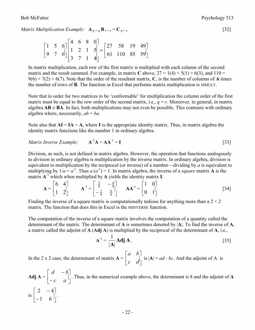
Matrix Multiplication Example: A p × q B r × s = C p × s [32]
1 5 6
9 7 6
4 6 8 0
1 2 1 5
3 7 1 4
27 58 19 49
61 110 85 59
In matrix multiplication, each row of the first matrix is multiplied with each column of the second matrix and the result summed. For example, in matrix C above, 27 = 1(4) + 5(1) + 6(3), and 110 = 9(6) + 7(2) + 6(7). Note that the order of the resultant matrix, C, is the number of columns of A times the number of rows of B. The function in Excel that performs matrix multiplication is MMULT.
Note that in order for two matrices to be ‘conformable’ for multiplication the column order of the first matrix must be equal to the row order of the second matrix, i.e., q = r. Moreover, in general, in matrix algebra AB ≠ BA. In fact, both multiplications may not even be possible. This contrasts with ordinary algebra where, necessarily, ab = ba.
Note also that AI = IA = A, where I is the appropriate identity matrix. Thus, in matrix algebra the identity matrix functions like the number 1 in ordinary algebra.
Matrix Inverse Example: A-1A = AA-1 = I [33]
Division, as such, is not defined in matrix algebra. However, the operation that functions analogously to division in ordinary algebra is multiplication by the inverse matrix. In ordinary algebra, division is equivalent to multiplication by the reciprocal (or inverse) of a number—dividing by a is equivalent to multiplying by 1/a = a-1. Thus a (a-1) = 1. In matrix algebra, the inverse of a square matrix A is the matrix A-1 which when multiplied by A yields the identity matrix I.
A = 6 4
1 2
A-1 =
28
48
18
68
AA-1 =
1 0
0 1
[34]
Finding the inverse of a square matrix is computationally tedious for anything more than a 2 × 2 matrix. The function that does this in Excel is the MINVERSE function.
The computation of the inverse of a square matrix involves the computation of a quantity called the determinant of the matrix. The determinant of A is sometimes denoted by |A|. To find the inverse of A, a matrix called the adjoint of A (Adj A) is multiplied by the reciprocal of the determinant of A, i.e.,
A-1 = 1
| |AAdj A . [35]
In the 2 x 2 case, the determinant of matrix A = a b
c d
is |A| = ad - bc. And the adjoint of A is
Adj A = d b
c a
. Thus, in the numerical example above, the determinant is 8 and the adjoint of A
is 2 4
1 6
.

Bob McFatter Psychology 513
- 23 -
Because computation of the inverse of a matrix involves division of numbers by the determinant of the matrix, the operation becomes undefined when the determinant of the matrix is zero. When a matrix has a determinant that is zero, the matrix is said to be singular, and its inverse does not exist.
Linear Dependence and the Rank of a Matrix
A matrix will be singular when its rows or columns are linearly dependent. For example, if one of the columns of a matrix can be expressed as an exact linear combination of the other columns of the matrix, then the columns are linearly dependent. The following matrix is singular (its determinant is zero) because its columns are linearly dependent. The third column is equal to 3 times the first column minus 2 times the second column.
A =
6 4 10
7 3 15
4 5 2
. No inverse exists for this matrix.
When the rows and columns of a matrix are not linearly dependent the matrix is said to be of full rank.If a matrix is not of full rank, then it is singular. The rank of a matrix is defined to be the maximum number of linearly independent columns (or rows) of the matrix. The matrix above is of rank 2 because only two of the columns are linearly independent. It can be shown that the rank of an r x c matrix cannot exceed the minimum of r and c. For example, the rank of a 6 x 10 matrix can at most be 6. Also, when two matrices are multiplied, the rank of the resulting matrix can be at most the rank of the matrix with the smallest rank. Linear dependence and rank become important in regression analysis because the computation of regression coefficients involves finding the inverse of a matrix. If that matrix is singular, no solution exists.
Basic Theorems from Matrix Algebra
Below are some basic theorems for manipulation of matrices in matrix algebra. I have reproduced these from Kutner et al., p. 193:
A + B = B + A(A + B) + C = A + (B + C)
(AB)C = A(BC)C(A + B) = CA + CBλ(A + B) = λA + λB (λ is any scalar)
(A')' = A(A + B)' = A' + B' [36]
(AB)' = B'A'(ABC)' = C'B'A'
(AB)-1 = B-1A-1
(ABC)-1 = C-1B-1A-1
(A-1)-1 = A(A')-1 = (A-1)'
Notice that a major difference between matrix algebra and ordinary algebra is that sequential order of
multiplication is crucial in matrix algebra whereas it is not in ordinary algebra.
Bob McFatter Psychology 513
- 24 -
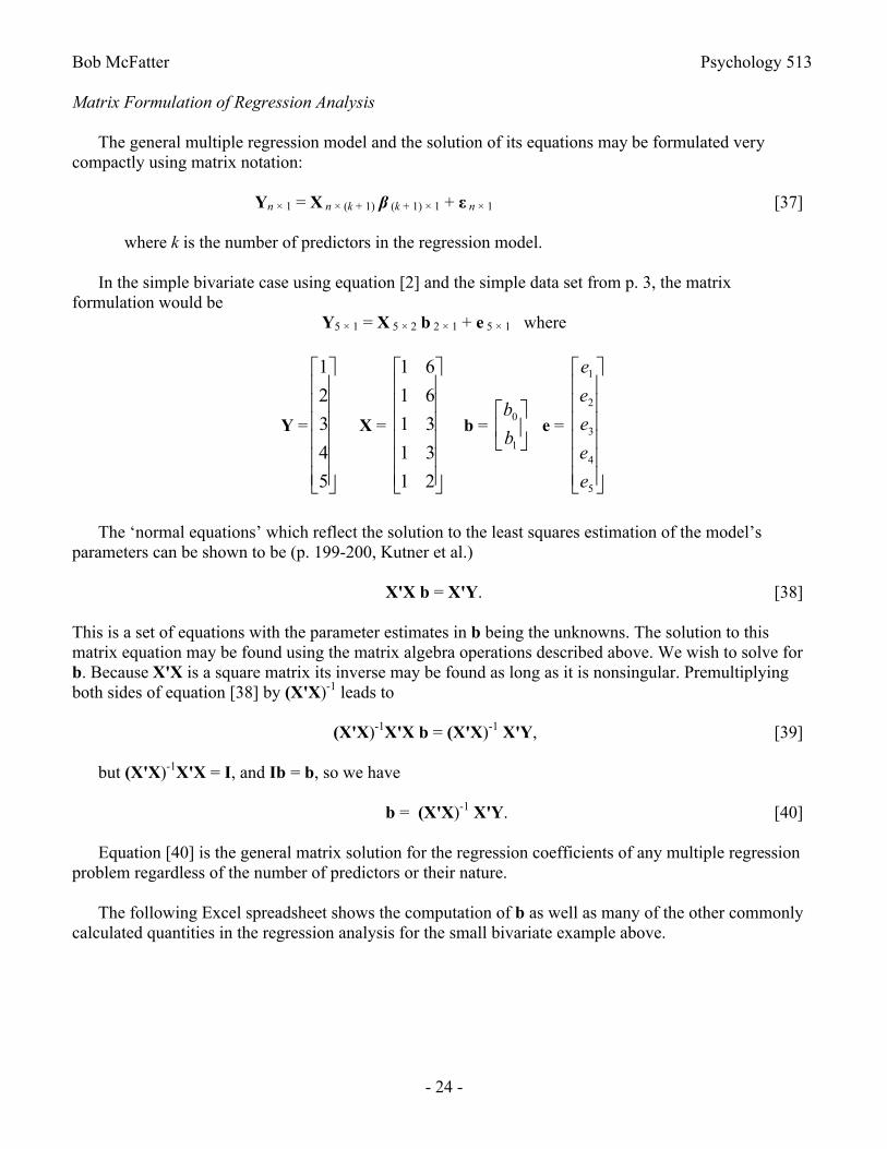
Matrix Formulation of Regression Analysis
The general multiple regression model and the solution of its equations may be formulated very compactly using matrix notation:
Yn × 1 = X n × (k + 1) β (k + 1) × 1 + ε n × 1 [37]
where k is the number of predictors in the regression model.
In the simple bivariate case using equation [2] and the simple data set from p. 3, the matrix formulation would be
Y5 × 1 = X 5 × 2 b 2 × 1 + e 5 × 1 where
Y =
1
2
3
4
5
X =
1 6
1 6
1 3
1 3
1 2
b = b
b0
1
e =
e
e
e
e
e
1
2
3
4
5
The ‘normal equations’ which reflect the solution to the least squares estimation of the model’s parameters can be shown to be (p. 199-200, Kutner et al.)
X'X b = X'Y. [38]
This is a set of equations with the parameter estimates in b being the unknowns. The solution to this matrix equation may be found using the matrix algebra operations described above. We wish to solve for b. Because X'X is a square matrix its inverse may be found as long as it is nonsingular. Premultiplying both sides of equation [38] by (X'X)-1 leads to
(X'X)-1X'X b = (X'X)-1 X'Y, [39]
but (X'X)-1X'X = I, and Ib = b, so we have
b = (X'X)-1 X'Y. [40]
Equation [40] is the general matrix solution for the regression coefficients of any multiple regression problem regardless of the number of predictors or their nature.
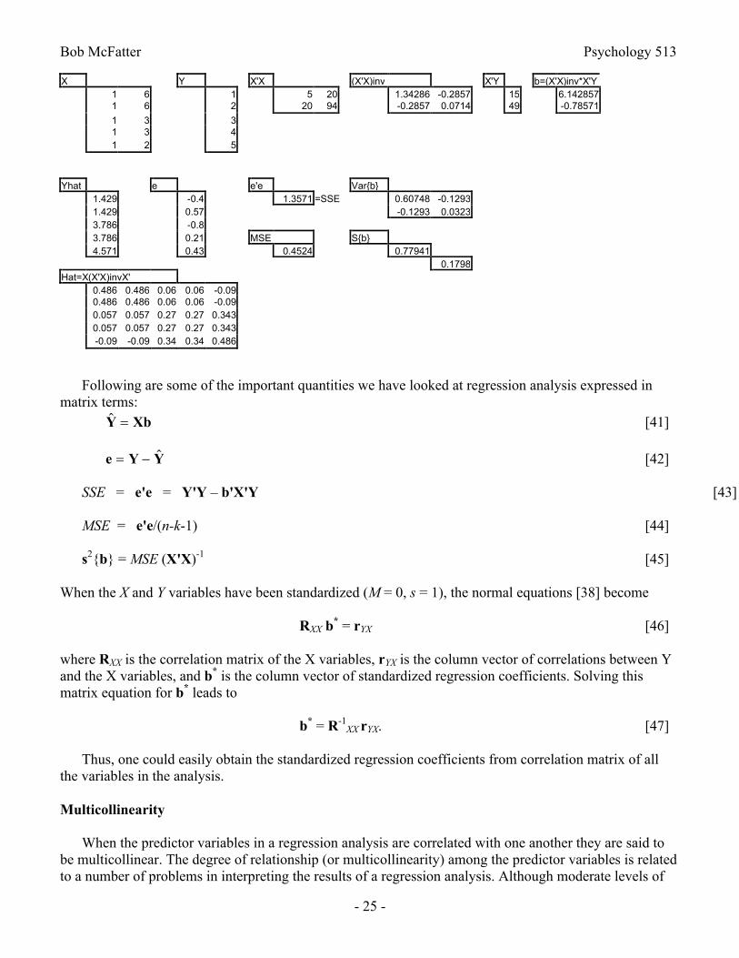
The following Excel spreadsheet shows the computation of b as well as many of the other commonly calculated quantities in the regression analysis for the small bivariate example above.
Bob McFatter Psychology 513
- 25 -
X Y X'X (X'X)inv X'Y b=(X'X)inv*X'Y1 6 1 5 20 1.34286 -0.2857 15 6.1428571 6 2 20 94 -0.2857 0.0714 49 -0.78571
1 3 31 3 41 2 5
Yhat e e'e Var{b}1.429 -0.4 1.3571 =SSE 0.60748 -0.12931.429 0.57 -0.1293 0.03233.786 -0.83.786 0.21 MSE S{b}4.571 0.43 0.4524 0.77941
0.1798Hat=X(X'X)invX'
0.486 0.486 0.06 0.06 -0.090.486 0.486 0.06 0.06 -0.090.057 0.057 0.27 0.27 0.3430.057 0.057 0.27 0.27 0.343-0.09 -0.09 0.34 0.34 0.486
Following are some of the important quantities we have looked at regression analysis expressed in matrix terms:
Y Xb [41]
e Y Y [42]
SSE = e'e = Y'Y – b'X'Y [43]
MSE = e'e/(n-k-1) [44]
s2{b} = MSE (X'X)-1 [45]
When the X and Y variables have been standardized (M = 0, s = 1), the normal equations [38] become
RXX b* = rYX [46]
where RXX is the correlation matrix of the X variables, rYX is the column vector of correlations between Y and the X variables, and b* is the column vector of standardized regression coefficients. Solving this matrix equation for b* leads to
b* = R-1XX rYX. [47]
Thus, one could easily obtain the standardized regression coefficients from correlation matrix of all the variables in the analysis.
Multicollinearity
When the predictor variables in a regression analysis are correlated with one another they are said to be multicollinear. The degree of relationship (or multicollinearity) among the predictor variables is related to a number of problems in interpreting the results of a regression analysis. Although moderate levels of
Bob McFatter Psychology 513
- 26 -
multicollinearity do not ordinarily produce major difficulties of interpretation, the multicollinearity does affect the interpretation of the equation, and extreme multicollinearity can make it impossible, or next to impossible, to even estimate the equation, let alone interpret it. It should be noted that some authors restrict use of the term ‘multicollinearity’ to these situations of extreme multicollinearity.
If the predictors are all uncorrelated with one another (i.e., no multicollinearity) then interpretation of the analysis is quite straightforward. The relative contribution that each variable makes to the prediction of the criterion variable is simply the square of the correlation of that predictor with the criterion, and the total R2 may be partitioned into components that unambiguously reflect the contribution of each predictor as equation [30] shows.
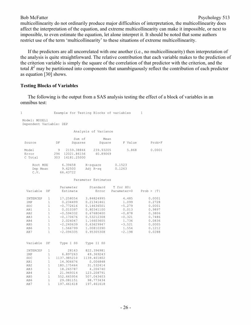
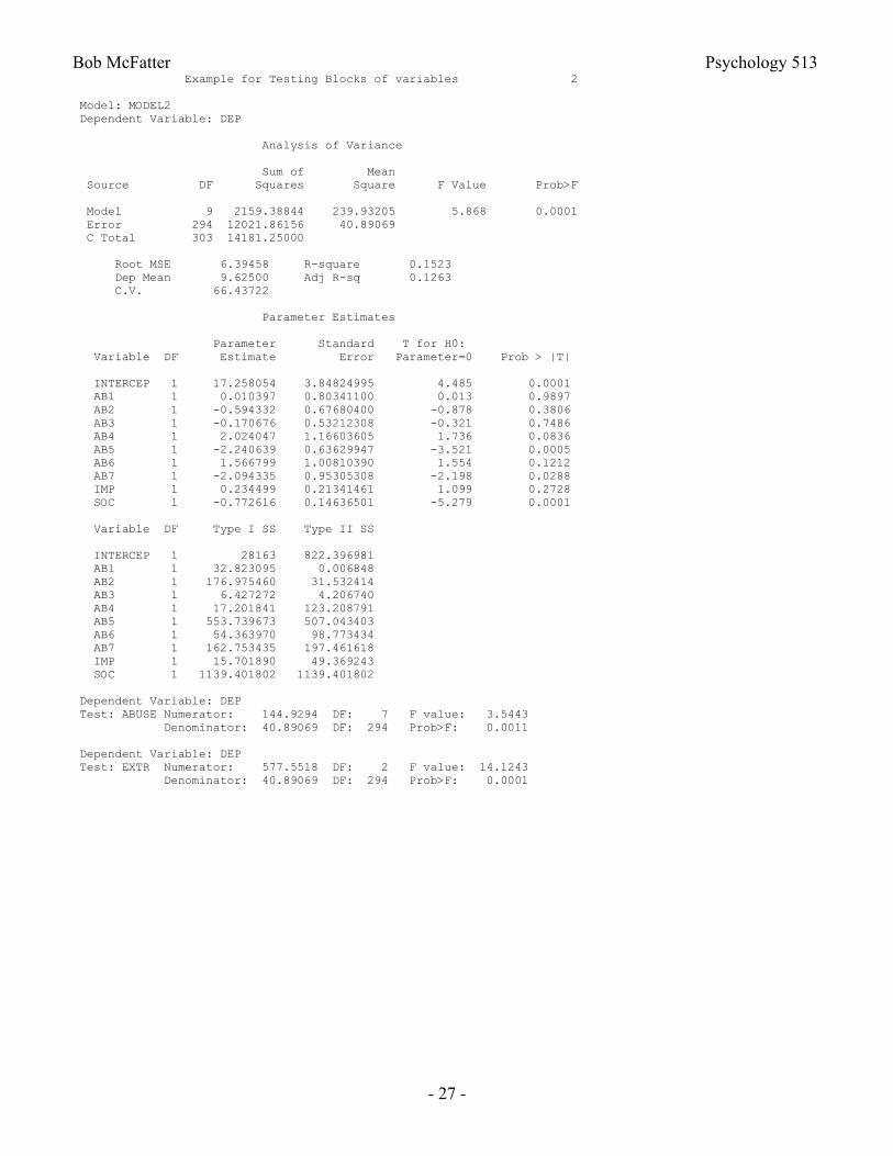
Testing Blocks of Variables
The following is the output from a SAS analysis testing the effect of a block of variables in an omnibus test:
1 Example for Testing Blocks of variables 1
Model: MODEL1 Dependent Variable: DEP
Analysis of Variance
Sum of Mean Source DF Squares Square F Value Prob>F
Model 9 2159.38844 239.93205 5.868 0.0001 Error 294 12021.86156 40.89069 C Total 303 14181.25000
Root MSE 6.39458 R-square 0.1523 Dep Mean 9.62500 Adj R-sq 0.1263 C.V. 66.43722
Parameter Estimates
Parameter Standard T for H0: Variable DF Estimate Error Parameter=0 Prob > |T|
INTERCEP 1 17.258054 3.84824995 4.485 0.0001 IMP 1 0.234499 0.21341461 1.099 0.2728 SOC 1 -0.772616 0.14636501 -5.279 0.0001 AB1 1 0.010397 0.80341100 0.013 0.9897 AB2 1 -0.594332 0.67680400 -0.878 0.3806 AB3 1 -0.170676 0.53212308 -0.321 0.7486 AB4 1 2.024047 1.16603605 1.736 0.0836 AB5 1 -2.240639 0.63629947 -3.521 0.0005 AB6 1 1.566799 1.00810390 1.554 0.1212 AB7 1 -2.094335 0.95305308 -2.198 0.0288
Variable DF Type I SS Type II SS
INTERCEP 1 28163 822.396981 IMP 1 6.897263 49.369243 SOC 1 1137.985210 1139.401802 AB1 1 14.906676 0.006848 AB2 1 180.175464 31.532414 AB3 1 18.265787 4.206740 AB4 1 21.949314 123.208791 AB5 1 552.665954 507.043403 AB6 1 29.081151 98.773434 AB7 1 197.461618 197.461618
Bob McFatter Psychology 513
- 27 -
Example for Testing Blocks of variables 2
Model: MODEL2 Dependent Variable: DEP
Analysis of Variance
Sum of Mean Source DF Squares Square F Value Prob>F
Model 9 2159.38844 239.93205 5.868 0.0001 Error 294 12021.86156 40.89069 C Total 303 14181.25000
Root MSE 6.39458 R-square 0.1523 Dep Mean 9.62500 Adj R-sq 0.1263 C.V. 66.43722
Parameter Estimates
Parameter Standard T for H0: Variable DF Estimate Error Parameter=0 Prob > |T|
INTERCEP 1 17.258054 3.84824995 4.485 0.0001 AB1 1 0.010397 0.80341100 0.013 0.9897 AB2 1 -0.594332 0.67680400 -0.878 0.3806 AB3 1 -0.170676 0.53212308 -0.321 0.7486 AB4 1 2.024047 1.16603605 1.736 0.0836 AB5 1 -2.240639 0.63629947 -3.521 0.0005 AB6 1 1.566799 1.00810390 1.554 0.1212 AB7 1 -2.094335 0.95305308 -2.198 0.0288 IMP 1 0.234499 0.21341461 1.099 0.2728 SOC 1 -0.772616 0.14636501 -5.279 0.0001
Variable DF Type I SS Type II SS
INTERCEP 1 28163 822.396981 AB1 1 32.823095 0.006848 AB2 1 176.975460 31.532414 AB3 1 6.427272 4.206740 AB4 1 17.201841 123.208791 AB5 1 553.739673 507.043403 AB6 1 54.363970 98.773434 AB7 1 162.753435 197.461618 IMP 1 15.701890 49.369243 SOC 1 1139.401802 1139.401802
Dependent Variable: DEP Test: ABUSE Numerator: 144.9294 DF: 7 F value: 3.5443 Denominator: 40.89069 DF: 294 Prob>F: 0.0011
Dependent Variable: DEP Test: EXTR Numerator: 577.5518 DF: 2 F value: 14.1243 Denominator: 40.89069 DF: 294 Prob>F: 0.0001
Bob McFatter Psychology 513
- 28 -
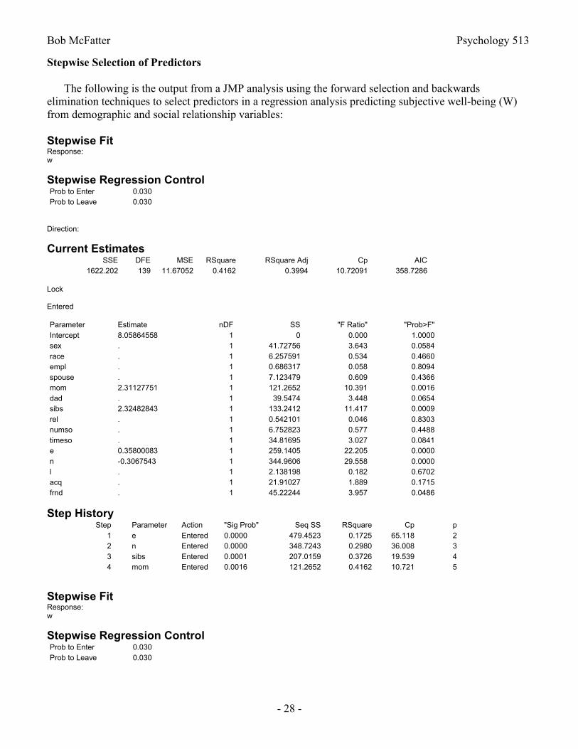
Stepwise Selection of Predictors
The following is the output from a JMP analysis using the forward selection and backwards elimination techniques to select predictors in a regression analysis predicting subjective well-being (W) from demographic and social relationship variables:
Stepwise FitResponse: w
Stepwise Regression ControlProb to Enter 0.030Prob to Leave 0.030
Direction:
Current EstimatesSSE DFE MSE RSquare RSquare Adj Cp AIC
1622.202 139 11.67052 0.4162 0.3994 10.72091 358.7286
Lock
Entered
Parameter Estimate nDF SS "F Ratio" "Prob>F"Intercept 8.05864558 1 0 0.000 1.0000sex . 1 41.72756 3.643 0.0584race . 1 6.257591 0.534 0.4660empl . 1 0.686317 0.058 0.8094spouse . 1 7.123479 0.609 0.4366mom 2.31127751 1 121.2652 10.391 0.0016dad . 1 39.5474 3.448 0.0654sibs 2.32482843 1 133.2412 11.417 0.0009rel . 1 0.542101 0.046 0.8303numso . 1 6.752823 0.577 0.4488timeso . 1 34.81695 3.027 0.0841e 0.35800083 1 259.1405 22.205 0.0000n -0.3067543 1 344.9606 29.558 0.0000l . 1 2.138198 0.182 0.6702acq . 1 21.91027 1.889 0.1715frnd . 1 45.22244 3.957 0.0486
Step HistoryStep Parameter Action "Sig Prob" Seq SS RSquare Cp p
1 e Entered 0.0000 479.4523 0.1725 65.118 22 n Entered 0.0000 348.7243 0.2980 36.008 33 sibs Entered 0.0001 207.0159 0.3726 19.539 44 mom Entered 0.0016 121.2652 0.4162 10.721 5
Stepwise FitResponse: w
Stepwise Regression ControlProb to Enter 0.030Prob to Leave 0.030
Bob McFatter Psychology 513
- 29 -
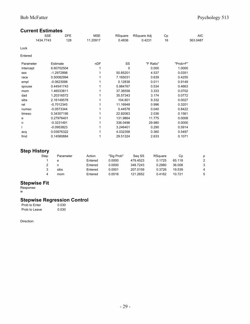
Current EstimatesSSE DFE MSE RSquare RSquare Adj Cp AIC
1434.7743 128 11.20917 0.4836 0.4231 16 363.0487
Lock
Entered
Parameter Estimate nDF SS "F Ratio" "Prob>F"Intercept 6.60702504 1 0 0.000 1.0000sex -1.2972898 1 50.85201 4.537 0.0351race 0.50082994 1 7.165031 0.639 0.4255empl -0.0623098 1 0.12838 0.011 0.9149spouse 0.44541743 1 5.984767 0.534 0.4663mom 1.46533811 1 37.36558 3.333 0.0702dad 1.20316572 1 35.57343 3.174 0.0772sibs 2.16149578 1 104.601 9.332 0.0027rel -0.7012345 1 11.16948 0.996 0.3201numso -0.0573344 1 0.44578 0.040 0.8422timeso 0.34307195 1 22.82063 2.036 0.1561e 0.27976401 1 131.9864 11.775 0.0008n -0.3231491 1 336.0496 29.980 0.0000l -0.0953823 1 3.246401 0.290 0.5914acq 0.03976322 1 4.032358 0.360 0.5497frnd 0.14580884 1 29.51324 2.633 0.1071
Step HistoryStep Parameter Action "Sig Prob" Seq SS RSquare Cp p
1 e Entered 0.0000 479.4523 0.1725 65.118 22 n Entered 0.0000 348.7243 0.2980 36.008 33 sibs Entered 0.0001 207.0159 0.3726 19.539 44 mom Entered 0.0016 121.2652 0.4162 10.721 5
Stepwise FitResponse: w
Stepwise Regression ControlProb to Enter 0.030Prob to Leave 0.030
Direction:

Bob McFatter Psychology 513
- 30 -
Current EstimatesSSE DFE MSE RSquare RSquare Adj Cp AIC
1521.3101 137 11.10445 0.4525 0.4285 5.720085 353.482
Entered
Parameter Estimate nDF SS "F Ratio" "Prob>F"Intercept 8.93337147 1 0 0.000 1.0000sex -1.2945208 1 55.66942 5.013 0.0268race . 1 7.209445 0.648 0.4224empl . 1 0.096685 0.009 0.9261spouse . 1 3.273621 0.293 0.5890mom 1.94450411 1 82.84942 7.461 0.0071dad . 1 36.98623 3.389 0.0678sibs 2.2709447 1 126.754 11.415 0.0009rel . 1 3.567762 0.320 0.5727numso . 1 0.000593 0.000 0.9942timeso . 1 25.4668 2.315 0.1304e 0.2798742 1 137.3623 12.370 0.0006n -0.3241244 1 380.7799 34.291 0.0000l . 1 2.254577 0.202 0.6539acq . 1 1.229298 0.110 0.7407frnd 0.18183481 1 59.16431 5.328 0.0225
Step HistoryStep Parameter Action "Sig Prob" Seq SS RSquare Cp p
1 e Entered 0.0000 479.4523 0.1725 65.118 22 n Entered 0.0000 348.7243 0.2980 36.008 33 sibs Entered 0.0001 207.0159 0.3726 19.539 44 mom Entered 0.0016 121.2652 0.4162 10.721 55 empl Removed 0.9149 0.12838 0.4836 14.011 156 numso Removed 0.8448 0.427913 0.4834 12.05 147 l Removed 0.5918 3.189925 0.4823 10.334 138 acq Removed 0.6265 2.612655 0.4814 8.5673 129 race Removed 0.5129 4.698999 0.4797 6.9865 11
10 spouse Removed 0.5187 4.551578 0.4780 5.3926 1011 rel Removed 0.2944 11.9927 0.4737 4.4625 912 timeso Removed 0.1569 21.9474 0.4658 4.4204 813 dad Removed 0.0678 36.98623 0.4525 5.7201 7
Bob McFatter Psychology 513
- 31 -
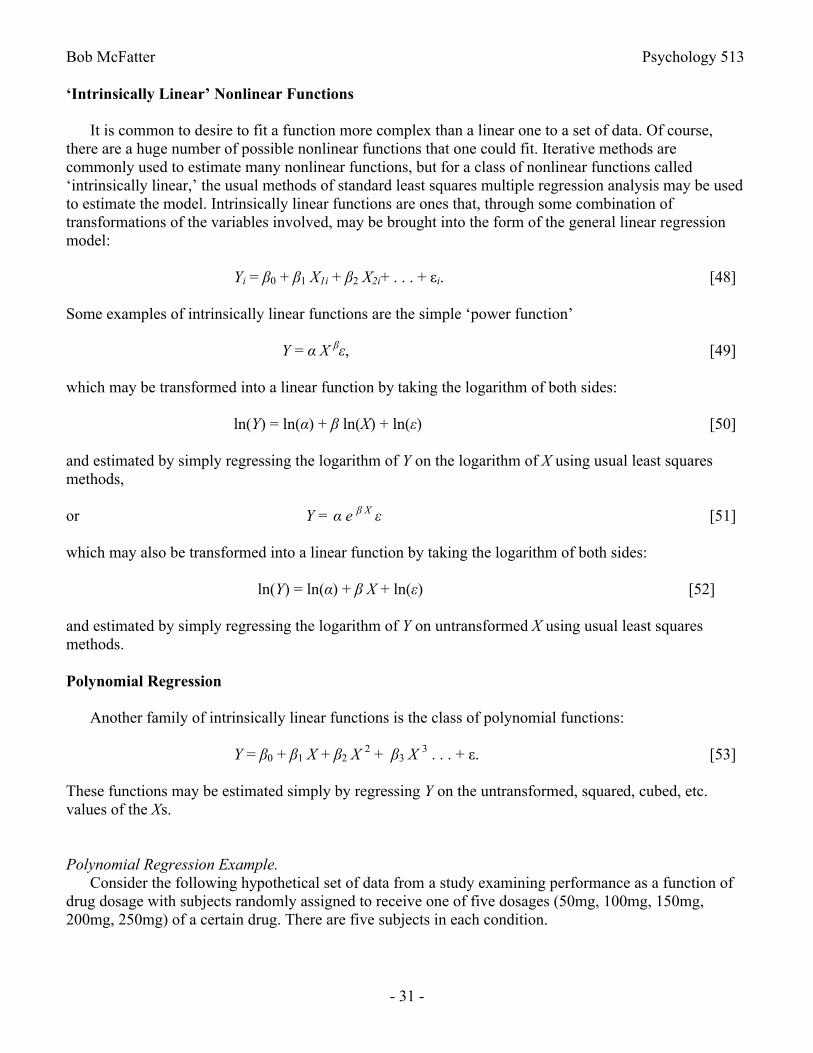
‘Intrinsically Linear’ Nonlinear Functions
It is common to desire to fit a function more complex than a linear one to a set of data. Of course, there are a huge number of possible nonlinear functions that one could fit. Iterative methods are commonly used to estimate many nonlinear functions, but for a class of nonlinear functions called ‘intrinsically linear,’ the usual methods of standard least squares multiple regression analysis may be used to estimate the model. Intrinsically linear functions are ones that, through some combination of transformations of the variables involved, may be brought into the form of the general linear regression model:
Yi = β0 + β1 X1i + β2 X2i+ . . . + εi. [48]
Some examples of intrinsically linear functions are the simple ‘power function’
Y = α X βε, [49]
which may be transformed into a linear function by taking the logarithm of both sides:
ln(Y) = ln(α) + β ln(X) + ln(ε) [50]
and estimated by simply regressing the logarithm of Y on the logarithm of X using usual least squares methods,
or Y = α e β X ε [51]
which may also be transformed into a linear function by taking the logarithm of both sides:
ln(Y) = ln(α) + β X + ln(ε) [52]
and estimated by simply regressing the logarithm of Y on untransformed X using usual least squares methods.
Polynomial Regression
Another family of intrinsically linear functions is the class of polynomial functions:
Y = β0 + β1 X + β2 X 2 + β3 X 3 . . . + ε. [53]
These functions may be estimated simply by regressing Y on the untransformed, squared, cubed, etc. values of the Xs.
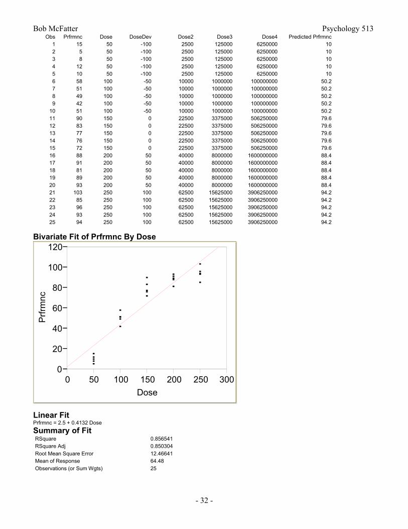
Polynomial Regression Example.Consider the following hypothetical set of data from a study examining performance as a function of
drug dosage with subjects randomly assigned to receive one of five dosages (50mg, 100mg, 150mg, 200mg, 250mg) of a certain drug. There are five subjects in each condition.
Bob McFatter Psychology 513
- 32 -
Obs Prfrmnc Dose DoseDev Dose2 Dose3 Dose4 Predicted Prfrmnc1 15 50 -100 2500 125000 6250000 102 5 50 -100 2500 125000 6250000 103 8 50 -100 2500 125000 6250000 104 12 50 -100 2500 125000 6250000 105 10 50 -100 2500 125000 6250000 106 58 100 -50 10000 1000000 100000000 50.27 51 100 -50 10000 1000000 100000000 50.28 49 100 -50 10000 1000000 100000000 50.29 42 100 -50 10000 1000000 100000000 50.2
10 51 100 -50 10000 1000000 100000000 50.211 90 150 0 22500 3375000 506250000 79.612 83 150 0 22500 3375000 506250000 79.613 77 150 0 22500 3375000 506250000 79.614 76 150 0 22500 3375000 506250000 79.615 72 150 0 22500 3375000 506250000 79.616 88 200 50 40000 8000000 1600000000 88.417 91 200 50 40000 8000000 1600000000 88.418 81 200 50 40000 8000000 1600000000 88.419 89 200 50 40000 8000000 1600000000 88.420 93 200 50 40000 8000000 1600000000 88.421 103 250 100 62500 15625000 3906250000 94.222 85 250 100 62500 15625000 3906250000 94.223 96 250 100 62500 15625000 3906250000 94.224 93 250 100 62500 15625000 3906250000 94.225 94 250 100 62500 15625000 3906250000 94.2
Bivariate Fit of Prfrmnc By Dose
0
20
40
60
80
100
120
Prf
rmnc
0 50 100 150 200 250 300
Dose
Linear FitPrfrmnc = 2.5 + 0.4132 Dose
Summary of FitRSquare 0.856541RSquare Adj 0.850304Root Mean Square Error 12.46641Mean of Response 64.48Observations (or Sum Wgts) 25
Bob McFatter Psychology 513
- 33 -
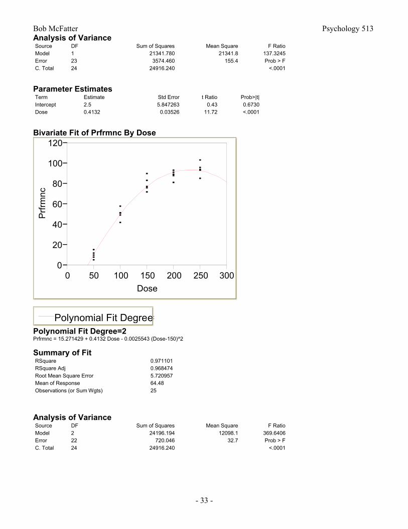
Analysis of VarianceSource DF Sum of Squares Mean Square F RatioModel 1 21341.780 21341.8 137.3245Error 23 3574.460 155.4 Prob > FC. Total 24 24916.240 <.0001
Parameter EstimatesTerm Estimate Std Error t Ratio Prob>|t|Intercept 2.5 5.847263 0.43 0.6730Dose 0.4132 0.03526 11.72 <.0001
Bivariate Fit of Prfrmnc By Dose
0
20
40
60
80
100
120
Prf
rmnc
0 50 100 150 200 250 300
Dose
Polynomial Fit Degree=2Polynomial Fit Degree=2Prfrmnc = 15.271429 + 0.4132 Dose - 0.0025543 (Dose-150)^2
Summary of FitRSquare 0.971101RSquare Adj 0.968474Root Mean Square Error 5.720957Mean of Response 64.48Observations (or Sum Wgts) 25
Analysis of VarianceSource DF Sum of Squares Mean Square F RatioModel 2 24196.194 12098.1 369.6406Error 22 720.046 32.7 Prob > FC. Total 24 24916.240 <.0001
Bob McFatter Psychology 513
- 34 -
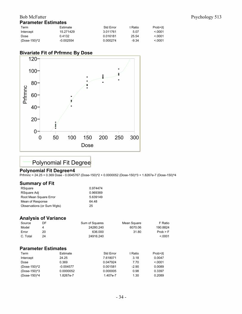
Parameter EstimatesTerm Estimate Std Error t Ratio Prob>|t|Intercept 15.271429 3.011761 5.07 <.0001Dose 0.4132 0.016181 25.54 <.0001(Dose-150)^2 -0.002554 0.000274 -9.34 <.0001
Bivariate Fit of Prfrmnc By Dose
0
20
40
60
80
100
120
Prf
rmnc
0 50 100 150 200 250 300
Dose
Polynomial Fit Degree=4Polynomial Fit Degree=4Prfrmnc = 24.25 + 0.369 Dose - 0.0045767 (Dose-150)^2 + 0.0000052 (Dose-150)^3 + 1.8267e-7 (Dose-150)^4
Summary of FitRSquare 0.974474RSquare Adj 0.969369Root Mean Square Error 5.639149Mean of Response 64.48Observations (or Sum Wgts) 25
Analysis of VarianceSource DF Sum of Squares Mean Square F RatioModel 4 24280.240 6070.06 190.8824Error 20 636.000 31.80 Prob > FC. Total 24 24916.240 <.0001
Parameter EstimatesTerm Estimate Std Error t Ratio Prob>|t|Intercept 24.25 7.618071 3.18 0.0047Dose 0.369 0.047924 7.70 <.0001(Dose-150)^2 -0.004577 0.001581 -2.90 0.0089(Dose-150)^3 0.0000052 0.000005 0.98 0.3397(Dose-150)^4 1.8267e-7 1.407e-7 1.30 0.2089
Bob McFatter Psychology 513
- 35 -
Bivariate Fit of Prfrmnc By Dose
0
20
40
60
80
100
120
Prf
rmnc
0 50 100 150 200 250 300
Dose
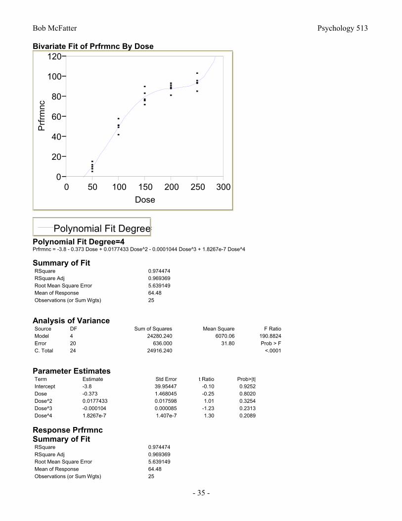
Polynomial Fit Degree=4Polynomial Fit Degree=4Prfrmnc = -3.8 - 0.373 Dose + 0.0177433 Dose^2 - 0.0001044 Dose^3 + 1.8267e-7 Dose^4
Summary of FitRSquare 0.974474RSquare Adj 0.969369Root Mean Square Error 5.639149Mean of Response 64.48Observations (or Sum Wgts) 25
Analysis of VarianceSource DF Sum of Squares Mean Square F RatioModel 4 24280.240 6070.06 190.8824Error 20 636.000 31.80 Prob > FC. Total 24 24916.240 <.0001
Parameter EstimatesTerm Estimate Std Error t Ratio Prob>|t|Intercept -3.8 39.95447 -0.10 0.9252Dose -0.373 1.468045 -0.25 0.8020Dose^2 0.0177433 0.017598 1.01 0.3254Dose^3 -0.000104 0.000085 -1.23 0.2313Dose^4 1.8267e-7 1.407e-7 1.30 0.2089
Response PrfrmncSummary of FitRSquare 0.974474RSquare Adj 0.969369Root Mean Square Error 5.639149Mean of Response 64.48Observations (or Sum Wgts) 25
Bob McFatter Psychology 513
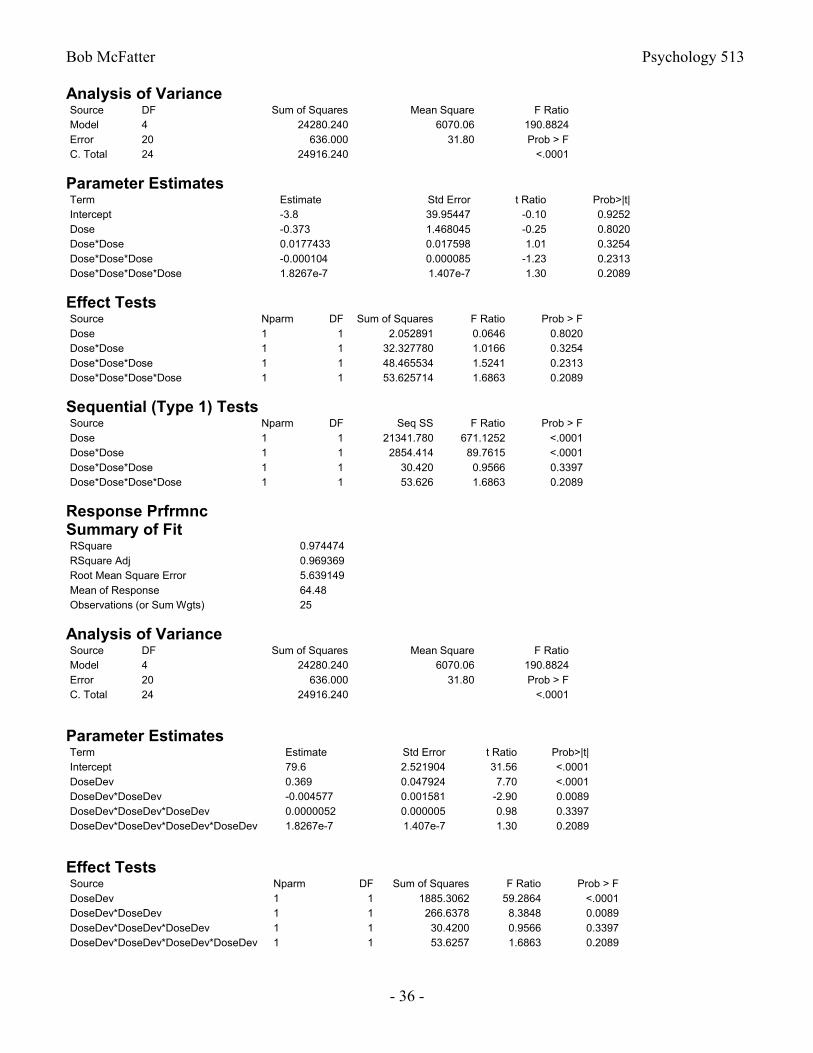
- 36 -
Analysis of VarianceSource DF Sum of Squares Mean Square F RatioModel 4 24280.240 6070.06 190.8824Error 20 636.000 31.80 Prob > FC. Total 24 24916.240 <.0001
Parameter EstimatesTerm Estimate Std Error t Ratio Prob>|t|Intercept -3.8 39.95447 -0.10 0.9252Dose -0.373 1.468045 -0.25 0.8020Dose*Dose 0.0177433 0.017598 1.01 0.3254Dose*Dose*Dose -0.000104 0.000085 -1.23 0.2313Dose*Dose*Dose*Dose 1.8267e-7 1.407e-7 1.30 0.2089
Effect TestsSource Nparm DF Sum of Squares F Ratio Prob > FDose 1 1 2.052891 0.0646 0.8020Dose*Dose 1 1 32.327780 1.0166 0.3254Dose*Dose*Dose 1 1 48.465534 1.5241 0.2313Dose*Dose*Dose*Dose 1 1 53.625714 1.6863 0.2089
Sequential (Type 1) TestsSource Nparm DF Seq SS F Ratio Prob > FDose 1 1 21341.780 671.1252 <.0001Dose*Dose 1 1 2854.414 89.7615 <.0001Dose*Dose*Dose 1 1 30.420 0.9566 0.3397Dose*Dose*Dose*Dose 1 1 53.626 1.6863 0.2089
Response PrfrmncSummary of FitRSquare 0.974474RSquare Adj 0.969369Root Mean Square Error 5.639149Mean of Response 64.48Observations (or Sum Wgts) 25
Analysis of VarianceSource DF Sum of Squares Mean Square F RatioModel 4 24280.240 6070.06 190.8824Error 20 636.000 31.80 Prob > FC. Total 24 24916.240 <.0001
Parameter EstimatesTerm Estimate Std Error t Ratio Prob>|t|Intercept 79.6 2.521904 31.56 <.0001DoseDev 0.369 0.047924 7.70 <.0001DoseDev*DoseDev -0.004577 0.001581 -2.90 0.0089DoseDev*DoseDev*DoseDev 0.0000052 0.000005 0.98 0.3397DoseDev*DoseDev*DoseDev*DoseDev 1.8267e-7 1.407e-7 1.30 0.2089
Effect TestsSource Nparm DF Sum of Squares F Ratio Prob > FDoseDev 1 1 1885.3062 59.2864 <.0001DoseDev*DoseDev 1 1 266.6378 8.3848 0.0089DoseDev*DoseDev*DoseDev 1 1 30.4200 0.9566 0.3397DoseDev*DoseDev*DoseDev*DoseDev 1 1 53.6257 1.6863 0.2089
Bob McFatter Psychology 513
- 37 -
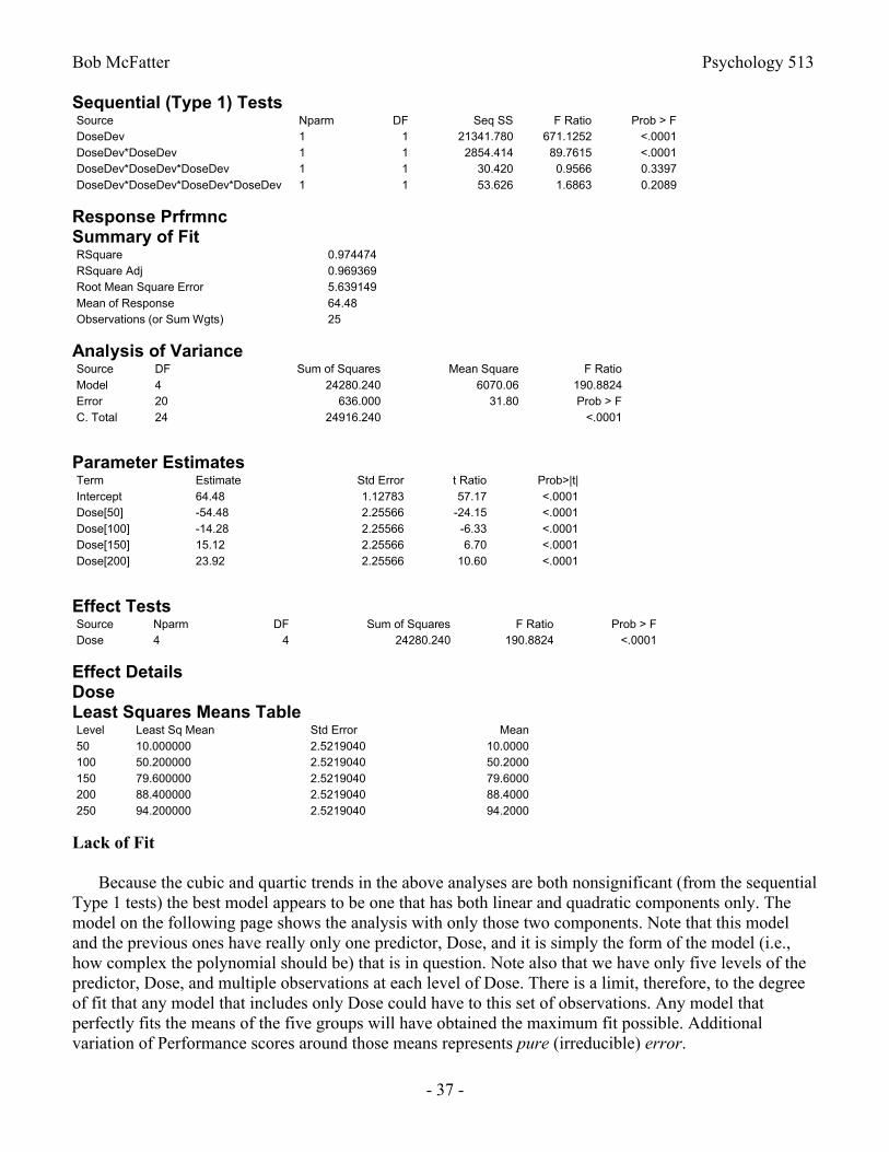
Sequential (Type 1) TestsSource Nparm DF Seq SS F Ratio Prob > FDoseDev 1 1 21341.780 671.1252 <.0001DoseDev*DoseDev 1 1 2854.414 89.7615 <.0001DoseDev*DoseDev*DoseDev 1 1 30.420 0.9566 0.3397DoseDev*DoseDev*DoseDev*DoseDev 1 1 53.626 1.6863 0.2089
Response PrfrmncSummary of FitRSquare 0.974474RSquare Adj 0.969369Root Mean Square Error 5.639149Mean of Response 64.48Observations (or Sum Wgts) 25
Analysis of VarianceSource DF Sum of Squares Mean Square F RatioModel 4 24280.240 6070.06 190.8824Error 20 636.000 31.80 Prob > FC. Total 24 24916.240 <.0001
Parameter EstimatesTerm Estimate Std Error t Ratio Prob>|t|Intercept 64.48 1.12783 57.17 <.0001Dose[50] -54.48 2.25566 -24.15 <.0001Dose[100] -14.28 2.25566 -6.33 <.0001Dose[150] 15.12 2.25566 6.70 <.0001Dose[200] 23.92 2.25566 10.60 <.0001
Effect TestsSource Nparm DF Sum of Squares F Ratio Prob > FDose 4 4 24280.240 190.8824 <.0001
Effect DetailsDoseLeast Squares Means TableLevel Least Sq Mean Std Error Mean50 10.000000 2.5219040 10.0000100 50.200000 2.5219040 50.2000150 79.600000 2.5219040 79.6000200 88.400000 2.5219040 88.4000250 94.200000 2.5219040 94.2000
Lack of Fit
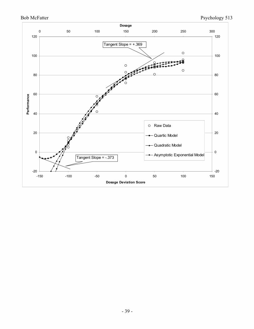
Because the cubic and quartic trends in the above analyses are both nonsignificant (from the sequential Type 1 tests) the best model appears to be one that has both linear and quadratic components only. The model on the following page shows the analysis with only those two components. Note that this model and the previous ones have really only one predictor, Dose, and it is simply the form of the model (i.e., how complex the polynomial should be) that is in question. Note also that we have only five levels of the predictor, Dose, and multiple observations at each level of Dose. There is a limit, therefore, to the degree of fit that any model that includes only Dose could have to this set of observations. Any model that perfectly fits the means of the five groups will have obtained the maximum fit possible. Additional variation of Performance scores around those means represents pure (irreducible) error.

Bob McFatter Psychology 513
- 38 -
It is common to evaluate how well a model fits a set of data by testing whether the error variation left over after the model fit is significantly greater than pure error. If this lack of fit error is not significant, then we conclude that the model is a good fit to the data. In the polynomial trend analysis example above, the pure error estimate would be the MSE for the quartic model that perfectly fits the five means. No model with only Dose as a predictor will do better than perfectly fitting the five means. Is the quadratic model (with only linear and quadratic components) a good fit to the data? The Lack of Fit section of the JMP output tests this by testing whether the block of two additional predictors that would lead to a perfect fit (cubic and quartic) significantly improves prediction over the linear and quadratic. Because it does not, F(2, 20) = 1.32, p = .2890, we conclude that the quadratic model is a good fit.
Response Prfrmnc Summary of FitRSquare 0.971101RSquare Adj 0.968474Root Mean Square Error 5.720957Mean of Response 64.48Observations (or Sum Wgts) 25
Analysis of VarianceSource DF Sum of Squares Mean Square F RatioModel 2 24196.194 12098.1 369.6406Error 22 720.046 32.7 Prob > FC. Total 24 24916.240 <.0001
Lack Of FitSource DF Sum of Squares Mean Square F RatioLack Of Fit 2 84.04571 42.0229 1.3215Pure Error 20 636.00000 31.8000 Prob > FTotal Error 22 720.04571 0.2890
Max RSq0.9745
Parameter EstimatesTerm Estimate Std Error t Ratio Prob>|t|Intercept 77.251429 1.783094 43.32 <.0001DoseD 0.4132 0.016181 25.54 <.0001DoseD*DoseD -0.002554 0.000274 -9.34 <.0001
Effect TestsSource Nparm DF Sum of Squares F Ratio Prob > FDoseD 1 1 21341.780 652.0685 <.0001DoseD*DoseD 1 1 2854.414 87.2127 <.0001
Bob McFatter Psychology 513
- 39 -
-20
0
20
40
60
80
100
120
-150 -100 -50 0 50 100 150
Dosage Deviation Score
Pe
rfo
rma
nc
e
-20
0
20
40
60
80
100
120
0 50 100 150 200 250 300
Dosage
Raw Data
Quartic Model
Quadratic Model
Asymptotic Exponential Model
Tangent Slope = +.369
Tangent Slope = -.373
Bob McFatter Psychology 513
- 40 -
Models with Cross-Product (Interaction) Terms
In the simple multiple regression model with two predictors,Y b b X b X 0 1 1 2 2 , [54]
it is important to notice that the value of b1, which is the conditional or partial effect of X1 on Y holding X2
constant, does not depend on the value at which one holds X2 constant. That is, the effect of X1 on Y is the same, namely, b1, whether X2 is held constant at a very low level or at a high level. This is clearly reflected in the parallel lines in the 3-D surface plot of the best-fitting plane (see the plot in the IQ, extraversion, sales success example above).
If one includes a cross-product term in the equation, however, the response surface is no longer a plane, but rather a warped surface with nonparallel lines in the 3-D plot. Such a model would be
Y b b X b X b X X 0 1 1 2 2 3 1 2 . [55]Notice that because X1 appears in the equation more than once, the conditional effect of X1 on Y, holding X2 constant, is not simply b1. It is easy to see what the conditional effect of X1 is, however, by simply algebraically rearranging the equation:
Y b b b X X b X 0 1 3 2 1 2 2 . [56]
Notice that the coefficient of X1 in this equation is the quantity (b1 + b3 X2). This quantity is the conditional effect of X1 on Y, holding X2 constant, and its value depends on the value of X2. If X2 is zero, then the effect of X1 is b1. However, if X2 = 1, for example, then the effect of X1 is b1 + b3. When the effect of one independent or predictor variable on the criterion depends on the level of a second predictor, the two predictors are said to interact. Thus, a model that contains a cross-product term is an interactionmodel, as opposed to a purely additive model.
The interaction effect works the same way for X2. A rearrangement of equation [55] isolating X2 leads to the conditional effect of X2 being (b2 + b3 X1).
Notice, in particular, what the implications of these considerations are for the interpretations of the three regression coefficients, b1, b2, and b3, and their significance tests. It is a common error for researchers to interpret b1 and b2 as ‘main effects’ similar to the main effects in an ANOVA. It is important to see exactly why in general that is not correct. As equation [56] shows, b1 is the conditional effect of X1 on Y, holding X2 constant at zero. Therefore, b1 only has a meaningful interpretation for individuals who have a score of zero on X2. If zero is not a possible score for X2, or a score of interest, then b1 and its significance test do not have much interpretive value. Certainly one could not interpret it as the ‘main effect’ or average or simple effect of X1. The same goes for b2.
The interpretation of b3 is much less problematic. It is how much the conditional effect (slope) of X1
on Y, holding X2 constant, changes as X2 increases by one unit. Notice that it is also how much the conditional effect (slope) of X2 on Y, holding X1 constant, changes as X1 increases by one unit.
The problems in interpreting b1 and b2 occur because of the presence of the higher order term, X1X2, in the equation as well as the fact that zero may not be an interesting or meaningful value for X1 and X2. The coefficients b1 and b2 become much more interpretable if one rescales X1 and X2 before the analysis so that zero becomes an interesting value for the two variables. The most common way to do this is to standardize X1 and X2 to have means of zero and standard deviations of one before computing the cross-product. When that is done, b1 becomes the effect of X1 on Y for individuals who are at the mean on X2. The significance test of b1 tests whether that conditional effect is different from zero.

Bob McFatter Psychology 513
- 41 -
In models that have higher order terms (e.g., cross-products, squared terms) it is crucial in interpreting the lower order coefficients to pay careful attention to what a zero on the variables means. Without meaningful zeros on the variables the lower order coefficients and their significance tests become uninterpretable. Consequently, I recommend that unless a variable has a naturally interesting and interpretable zero, it should be standardized (or at least centered) prior to making cross-products or higher order terms in a regression model.
It is important to recognize that this procedure is not the same as simply doing a raw score regression analysis with higher order terms and then looking at the standardized regression weights from the analysis. The standardized regression weights from such an analysis are uninterpretable. This abominable practice is, unfortunately, all too common in the literature.
It is also important for interpretability of the coefficients that if a higher order term is in the model (e.g., X1X2), then all the components of the higher order term must also be in the model as lower order terms.
Extended Example. Predicting Subjective Well-being (W) from Extraversion (E) and Neuroticism (N).
Response WSummary of FitRSquare 0.353161RSquare Adj 0.349765Root Mean Square Error 3.860245Mean of Response 16.54427Observations (or Sum Wgts) 384
Analysis of VarianceSource DF Sum of Squares Mean Square F RatioModel 2 3099.7785 1549.89 104.0090Error 381 5677.4689 14.90 Prob > FC. Total 383 8777.2474 <.0001
Lack Of FitSource DF Sum of Squares Mean Square F RatioLack Of Fit 209 3012.5404 14.4141 0.9303Pure Error 172 2664.9286 15.4938 Prob > FTotal Error 381 5677.4689 0.6917
Max RSq0.6964
Parameter EstimatesTerm Estimate Std Error t Ratio Prob>|t|Intercept 16.544271 0.196992 83.98 <.0001Std E 1.9318696 0.198589 9.73 <.0001Std N -1.87633 0.198589 -9.45 <.0001
Response WSummary of FitRSquare 0.366178RSquare Adj 0.359488Root Mean Square Error 3.831274Mean of Response 16.54427Observations (or Sum Wgts) 384
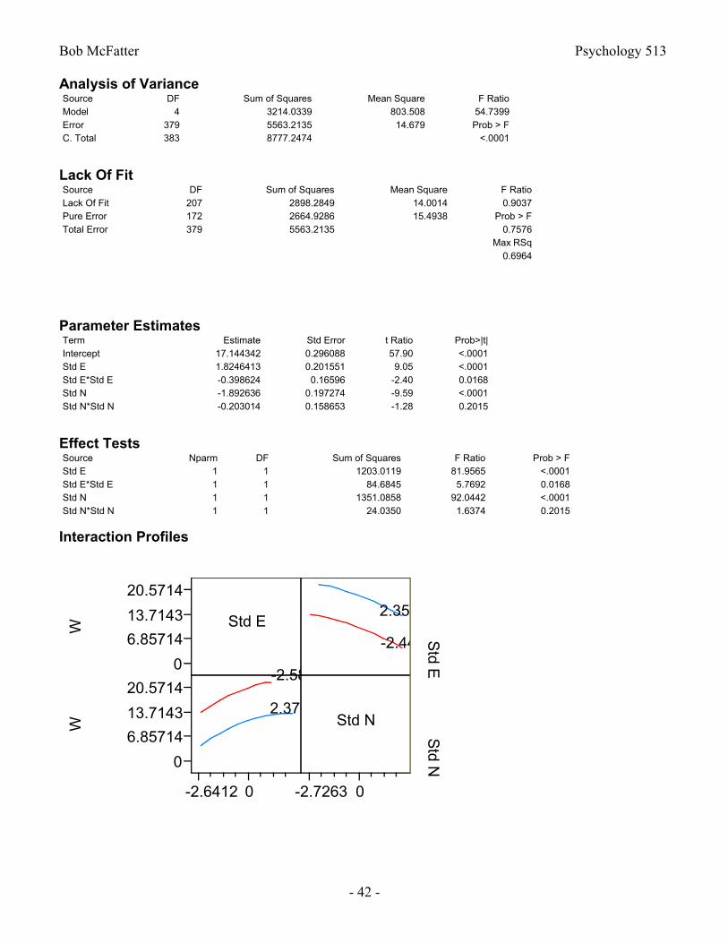
Bob McFatter Psychology 513
- 42 -
Analysis of VarianceSource DF Sum of Squares Mean Square F RatioModel 4 3214.0339 803.508 54.7399Error 379 5563.2135 14.679 Prob > FC. Total 383 8777.2474 <.0001
Lack Of FitSource DF Sum of Squares Mean Square F RatioLack Of Fit 207 2898.2849 14.0014 0.9037Pure Error 172 2664.9286 15.4938 Prob > FTotal Error 379 5563.2135 0.7576
Max RSq0.6964
Parameter EstimatesTerm Estimate Std Error t Ratio Prob>|t|Intercept 17.144342 0.296088 57.90 <.0001Std E 1.8246413 0.201551 9.05 <.0001Std E*Std E -0.398624 0.16596 -2.40 0.0168Std N -1.892636 0.197274 -9.59 <.0001Std N*Std N -0.203014 0.158653 -1.28 0.2015
Effect TestsSource Nparm DF Sum of Squares F Ratio Prob > FStd E 1 1 1203.0119 81.9565 <.0001Std E*Std E 1 1 84.6845 5.7692 0.0168Std N 1 1 1351.0858 92.0442 <.0001Std N*Std N 1 1 24.0350 1.6374 0.2015
Interaction Profiles
0
6.85714
13.7143
20.5714
W
0
6.85714
13.7143
20.5714
W
Std E
-2.581
2.3763
-2.6412 0
-2.443
2.3596
Std N
-2.7263 0
Std E
Std N
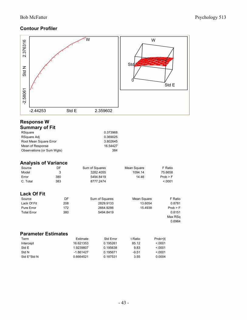
Bob McFatter Psychology 513
- 43 -
Contour Profiler2.
3763
16S
td N
-2.5
8061
W
-2.44253 Std E 2.359602
0Std E
Std N
W
Response WSummary of FitRSquare 0.373968RSquare Adj 0.369025Root Mean Square Error 3.802645Mean of Response 16.54427Observations (or Sum Wgts) 384
Analysis of VarianceSource DF Sum of Squares Mean Square F RatioModel 3 3282.4055 1094.14 75.6658Error 380 5494.8419 14.46 Prob > FC. Total 383 8777.2474 <.0001
Lack Of FitSource DF Sum of Squares Mean Square F RatioLack Of Fit 208 2829.9133 13.6054 0.8781Pure Error 172 2664.9286 15.4938 Prob > FTotal Error 380 5494.8419 0.8151
Max RSq0.6964
Parameter EstimatesTerm Estimate Std Error t Ratio Prob>|t|Intercept 16.621353 0.195261 85.12 <.0001Std E 1.9239807 0.195638 9.83 <.0001Std N -1.861427 0.195671 -9.51 <.0001Std E*Std N 0.6664521 0.187531 3.55 0.0004

Bob McFatter Psychology 513
- 44 -
Interaction Profiles
0
6.85714
13.7143
20.5714
W
0
6.85714
13.7143
20.5714
W
Std E
-2.5812.3763
-2.6412 0
-2.443
2.3596
Std N
-2.7263 0S
td ES
td N
Contour Profiler
2.37
6316
Std
N-2
.580
61
W
-2.44253 Std E 2.359602
0Std E
Std N
W
Response WSummary of FitRSquare 0.383923RSquare Adj 0.375773Root Mean Square Error 3.782256Mean of Response 16.54427Observations (or Sum Wgts) 384
Analysis of VarianceSource DF Sum of Squares Mean Square F RatioModel 5 3369.7836 673.957 47.1119Error 378 5407.4638 14.305 Prob > FC. Total 383 8777.2474 <.0001
Lack Of FitSource DF Sum of Squares Mean Square F RatioLack Of Fit 206 2742.5352 13.3133 0.8593Pure Error 172 2664.9286 15.4938 Prob > FTotal Error 378 5407.4638 0.8516
Max RSq0.6964
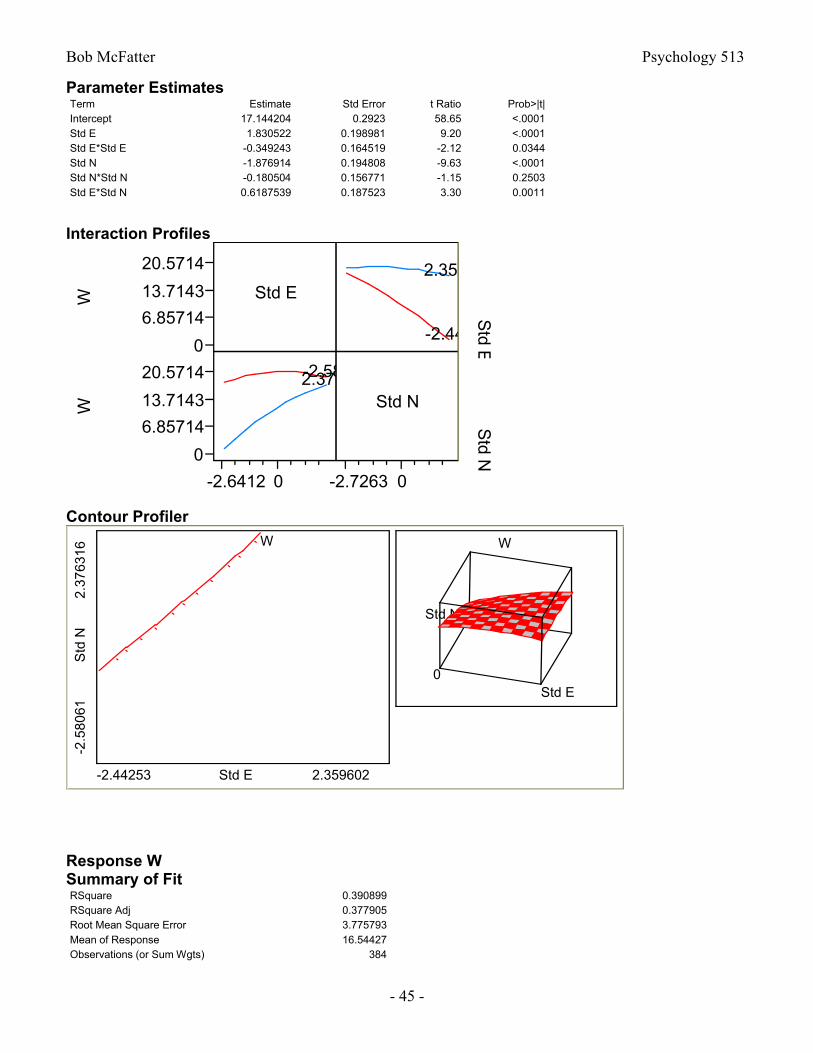
Bob McFatter Psychology 513
- 45 -
Parameter EstimatesTerm Estimate Std Error t Ratio Prob>|t|Intercept 17.144204 0.2923 58.65 <.0001Std E 1.830522 0.198981 9.20 <.0001Std E*Std E -0.349243 0.164519 -2.12 0.0344Std N -1.876914 0.194808 -9.63 <.0001Std N*Std N -0.180504 0.156771 -1.15 0.2503Std E*Std N 0.6187539 0.187523 3.30 0.0011
Interaction Profiles
0
6.85714
13.7143
20.5714
W
0
6.85714
13.7143
20.5714
W
Std E
-2.5812.3763
-2.6412 0
-2.443
2.3596
Std N
-2.7263 0
Std E
Std N
Contour Profiler
2.37
6316
Std
N-2
.580
61
W
-2.44253 Std E 2.359602
0Std E
Std N
W
Response WSummary of FitRSquare 0.390899RSquare Adj 0.377905Root Mean Square Error 3.775793Mean of Response 16.54427Observations (or Sum Wgts) 384
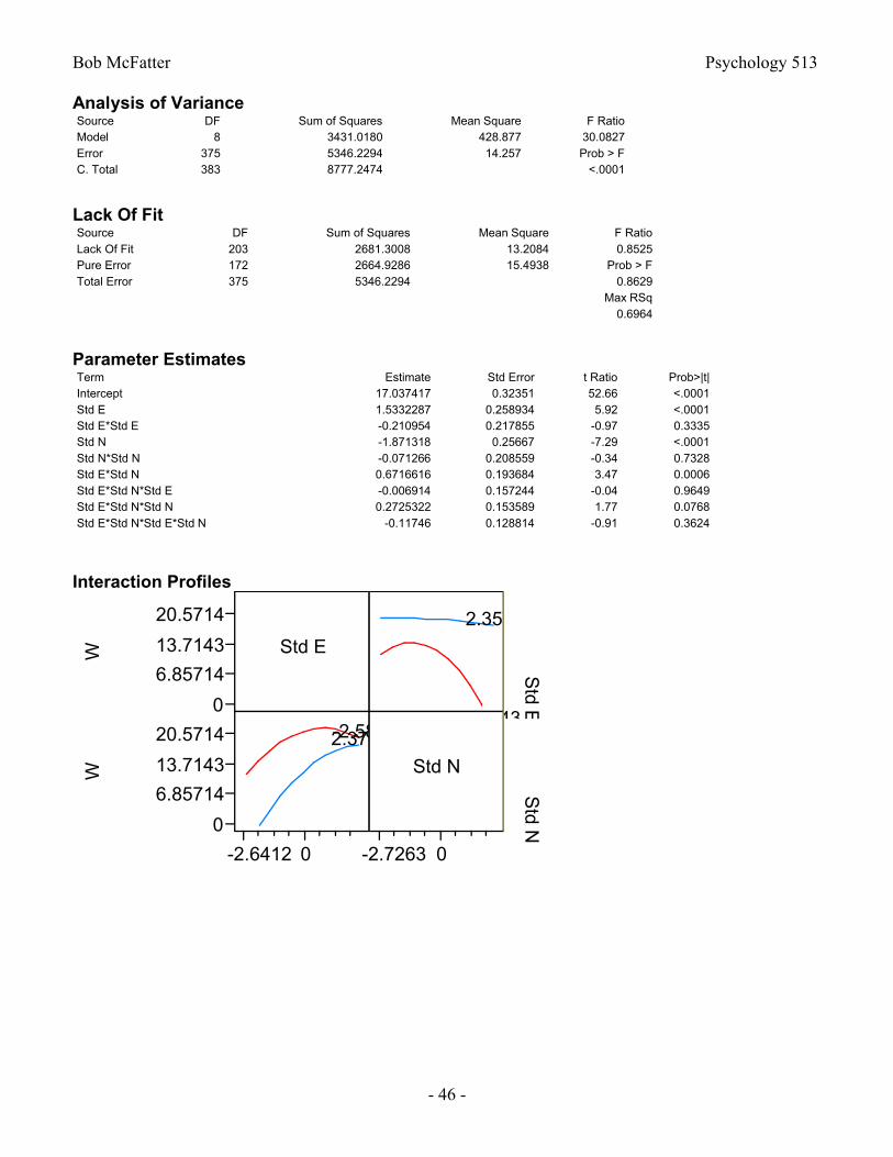
Bob McFatter Psychology 513
- 46 -
Analysis of VarianceSource DF Sum of Squares Mean Square F RatioModel 8 3431.0180 428.877 30.0827Error 375 5346.2294 14.257 Prob > FC. Total 383 8777.2474 <.0001
Lack Of FitSource DF Sum of Squares Mean Square F RatioLack Of Fit 203 2681.3008 13.2084 0.8525Pure Error 172 2664.9286 15.4938 Prob > FTotal Error 375 5346.2294 0.8629
Max RSq0.6964
Parameter EstimatesTerm Estimate Std Error t Ratio Prob>|t|Intercept 17.037417 0.32351 52.66 <.0001Std E 1.5332287 0.258934 5.92 <.0001Std E*Std E -0.210954 0.217855 -0.97 0.3335Std N -1.871318 0.25667 -7.29 <.0001Std N*Std N -0.071266 0.208559 -0.34 0.7328Std E*Std N 0.6716616 0.193684 3.47 0.0006Std E*Std N*Std E -0.006914 0.157244 -0.04 0.9649Std E*Std N*Std N 0.2725322 0.153589 1.77 0.0768Std E*Std N*Std E*Std N -0.11746 0.128814 -0.91 0.3624
Interaction Profiles
0
6.85714
13.7143
20.5714
W
0
6.85714
13.7143
20.5714
W
Std E
-2.5812.3763
-2.6412 0
-2.443
2.3596
Std N
-2.7263 0
Std E
Std N
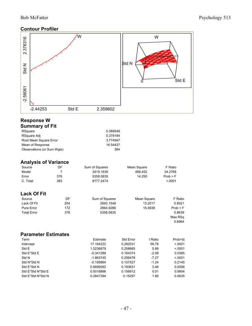
Bob McFatter Psychology 513
- 47 -
Contour Profiler2.
3763
16S
td N
-2.5
8061
W
-2.44253 Std E 2.359602
0 Std E
Std N
W
Response WSummary of FitRSquare 0.389549RSquare Adj 0.378184Root Mean Square Error 3.774947Mean of Response 16.54427Observations (or Sum Wgts) 384
Analysis of VarianceSource DF Sum of Squares Mean Square F RatioModel 7 3419.1639 488.452 34.2768Error 376 5358.0835 14.250 Prob > FC. Total 383 8777.2474 <.0001
Lack Of FitSource DF Sum of Squares Mean Square F RatioLack Of Fit 204 2693.1549 13.2017 0.8521Pure Error 172 2664.9286 15.4938 Prob > FTotal Error 376 5358.0835 0.8639
Max RSq0.6964
Parameter EstimatesTerm Estimate Std Error t Ratio Prob>|t|Intercept 17.164222 0.292031 58.78 <.0001Std E 1.5236879 0.258665 5.89 <.0001Std E*Std E -0.341289 0.164374 -2.08 0.0385Std N -1.863745 0.256478 -7.27 <.0001Std N*Std N -0.195864 0.157527 -1.24 0.2145Std E*Std N 0.6699262 0.193631 3.46 0.0006Std E*Std N*Std E 0.0018896 0.156912 0.01 0.9904Std E*Std N*Std N 0.2847394 0.15297 1.86 0.0635
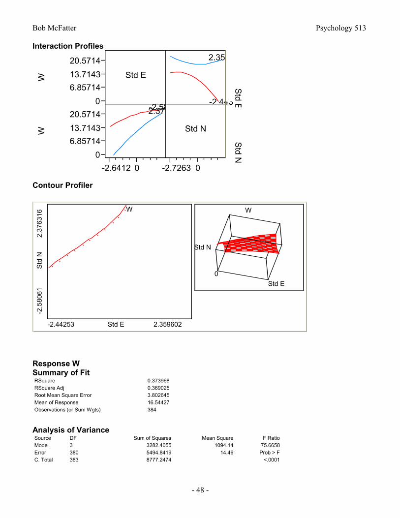
Bob McFatter Psychology 513
- 48 -
Interaction Profiles
0
6.85714
13.7143
20.5714
W
0
6.85714
13.7143
20.5714
W
Std E
-2.5812.3763
-2.6412 0
-2.443
2.3596
Std N
-2.7263 0S
td ES
td N
Contour Profiler
2.37
6316
Std
N-2
.580
61
W
-2.44253 Std E 2.359602
0
Std E
Std N
W
Response WSummary of FitRSquare 0.373968RSquare Adj 0.369025Root Mean Square Error 3.802645Mean of Response 16.54427Observations (or Sum Wgts) 384
Analysis of VarianceSource DF Sum of Squares Mean Square F RatioModel 3 3282.4055 1094.14 75.6658Error 380 5494.8419 14.46 Prob > FC. Total 383 8777.2474 <.0001
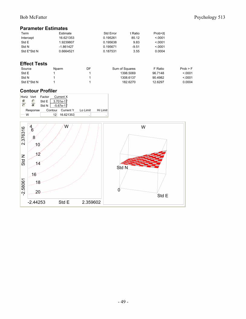
Bob McFatter Psychology 513
- 49 -
Parameter EstimatesTerm Estimate Std Error t Ratio Prob>|t|Intercept 16.621353 0.195261 85.12 <.0001Std E 1.9239807 0.195638 9.83 <.0001Std N -1.861427 0.195671 -9.51 <.0001Std E*Std N 0.6664521 0.187531 3.55 0.0004
Effect TestsSource Nparm DF Sum of Squares F Ratio Prob > FStd E 1 1 1398.5069 96.7148 <.0001Std N 1 1 1308.6137 90.4982 <.0001Std E*Std N 1 1 182.6270 12.6297 0.0004
Contour ProfilerHoriz Vert
Std EStd N
Factor
3.701e-17-5.67e-17
Current X
W
Response
12
Contour
16.621353
Current Y
.
Lo Limit
.
Hi Limit
2.37
6316
Std
N-2
.580
61
W
20
18
16
14
12
10
8
64
-2.44253 Std E 2.359602
0Std E
Std N
W
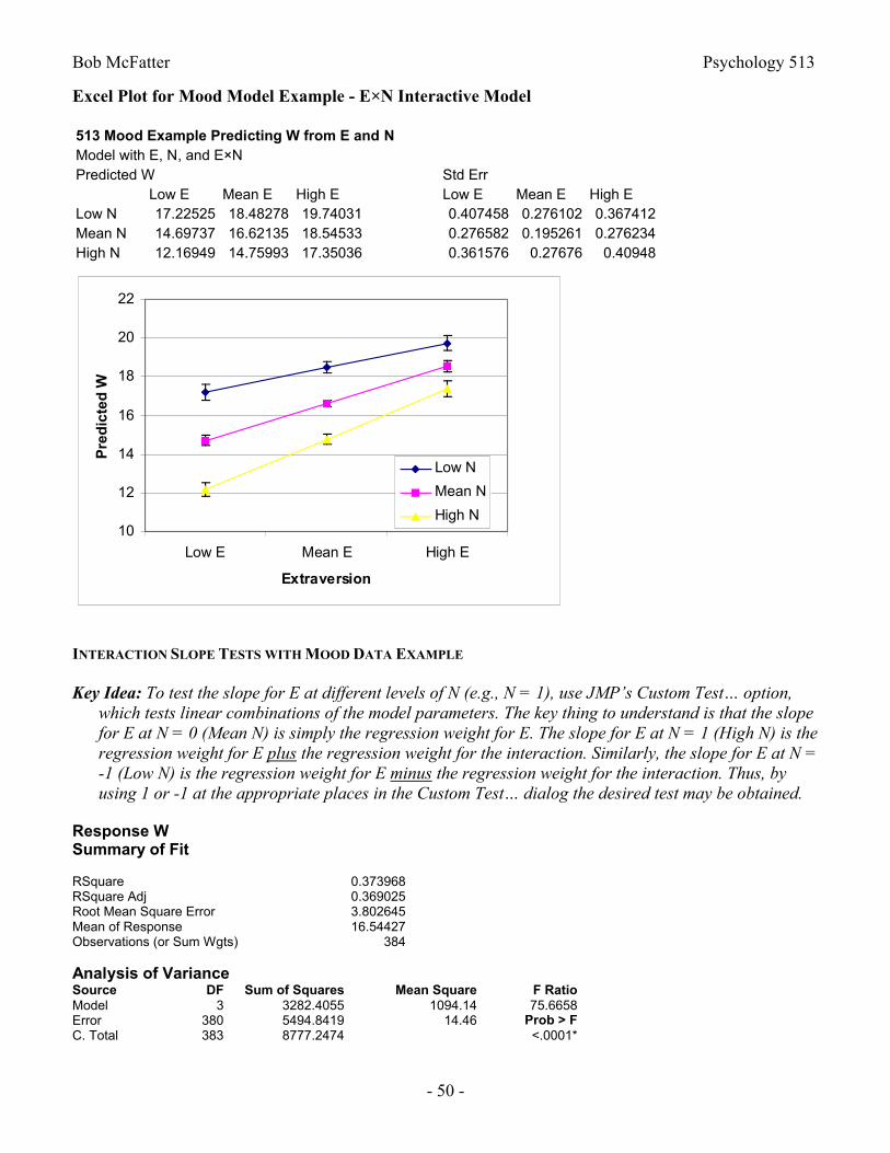
Bob McFatter Psychology 513
- 50 -
Excel Plot for Mood Model Example - E×N Interactive Model
513 Mood Example Predicting W from E and NModel with E, N, and E×NPredicted W Std Err
Low E Mean E High E Low E Mean E High ELow N 17.22525 18.48278 19.74031 0.407458 0.276102 0.367412Mean N 14.69737 16.62135 18.54533 0.276582 0.195261 0.276234High N 12.16949 14.75993 17.35036 0.361576 0.27676 0.40948
INTERACTION SLOPE TESTS WITH MOOD DATA EXAMPLE
Key Idea: To test the slope for E at different levels of N (e.g., N = 1), use JMP’s Custom Test… option, which tests linear combinations of the model parameters. The key thing to understand is that the slope for E at N = 0 (Mean N) is simply the regression weight for E. The slope for E at N = 1 (High N) is the regression weight for E plus the regression weight for the interaction. Similarly, the slope for E at N = -1 (Low N) is the regression weight for E minus the regression weight for the interaction. Thus, by using 1 or -1 at the appropriate places in the Custom Test… dialog the desired test may be obtained.
Response WSummary of Fit
RSquare 0.373968RSquare Adj 0.369025Root Mean Square Error 3.802645Mean of Response 16.54427Observations (or Sum Wgts) 384
Analysis of VarianceSource DF Sum of Squares Mean Square F RatioModel 3 3282.4055 1094.14 75.6658Error 380 5494.8419 14.46 Prob > FC. Total 383 8777.2474 <.0001*
10
12
14
16
18
20
22
Low E Mean E High E
Extraversion
Pre
dic
ted
W
Low N
Mean N
High N
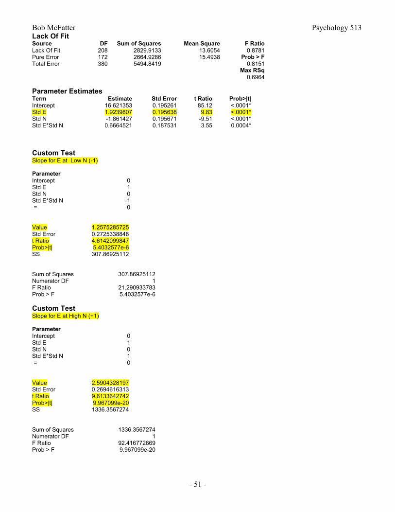
Bob McFatter Psychology 513
- 51 -
Lack Of FitSource DF Sum of Squares Mean Square F RatioLack Of Fit 208 2829.9133 13.6054 0.8781Pure Error 172 2664.9286 15.4938 Prob > FTotal Error 380 5494.8419 0.8151
Max RSq0.6964
Parameter EstimatesTerm Estimate Std Error t Ratio Prob>|t|Intercept 16.621353 0.195261 85.12 <.0001*Std E 1.9239807 0.195638 9.83 <.0001*Std N -1.861427 0.195671 -9.51 <.0001*Std E*Std N 0.6664521 0.187531 3.55 0.0004*
Custom TestSlope for E at Low N (-1)
ParameterIntercept 0Std E 1Std N 0Std E*Std N -1 = 0
Value 1.2575285725Std Error 0.2725338848t Ratio 4.6142099847Prob>|t| 5.4032577e-6SS 307.86925112
Sum of Squares 307.86925112Numerator DF 1F Ratio 21.290933783Prob > F 5.4032577e-6
Custom TestSlope for E at High N (+1)
ParameterIntercept 0Std E 1Std N 0Std E*Std N 1 = 0
Value 2.5904328197Std Error 0.2694616313t Ratio 9.6133642742Prob>|t| 9.967099e-20SS 1336.3567274
Sum of Squares 1336.3567274Numerator DF 1F Ratio 92.416772669Prob > F 9.967099e-20
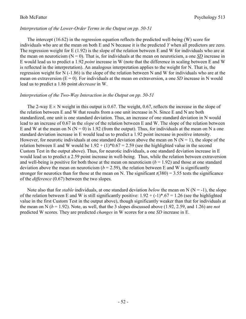
Bob McFatter Psychology 513
- 52 -
Interpretation of the Lower-Order Terms in the Output on pp. 50-51
The intercept (16.62) in the regression equation reflects the predicted well-being (W) score for individuals who are at the mean on both E and N because it is the predicted Y when all predictors are zero. The regression weight for E (1.92) is the slope of the relation between E and W for individuals who are at the mean on neuroticism (N = 0). That is, for individuals at the mean on neuroticism, a one SD increase in E would lead us to predict a 1.92 point increase in W (note that the difference in scaling between E and W is reflected in the interpretation). An analogous interpretation applies to the weight for N. That is, the regression weight for N (-1.86) is the slope of the relation between N and W for individuals who are at the mean on extraversion (E = 0). For individuals at the mean on extraversion, a one SD increase in N would lead us to predict a 1.86 point decrease in W.
Interpretation of the Two-Way Interaction in the Output on pp. 50-51
The 2-way E N weight in this output is 0.67. The weight, 0.67, reflects the increase in the slope of the relation between E and W that results from a one unit increase in N. Since E and N are both standardized, one unit is one standard deviation. Thus, an increase of one standard deviation in N would lead to an increase of 0.67 in the slope of the relation between E and W. The slope of the relation between E and W at the mean on N (N = 0) is 1.92 (from the output). Thus, for individuals at the mean on N a one standard deviation increase in E would lead us to predict a 1.92 point increase in positive intensity. However, for neurotic individuals at one standard deviation above the mean on N (N = 1), the slope of the relation between E and W would be 1.92 + (1)*0.67 = 2.59 (see the highlighted value in the second Custom Test in the output above). Thus, for neurotic individuals, a one standard deviation increase in E would lead us to predict a 2.59 point increase in well-being. Thus, while the relation between extraversion and well-being is positive for both those at the mean on neuroticism (b = 1.92) and those at one standard deviation above the mean on neuroticism (b = 2.59), the relation between E and W is significantly stronger for neurotics than for those at the mean on N. The significant t(380) = 3.55 tests the significance of the difference (0.67) between the two slopes.
Note also that for stable individuals, at one standard deviation below the mean on N (N = -1), the slope of the relation between E and W is still significantly positive: 1.92 + (-1)*.67 = 1.26 (see the highlighted value in the first Custom Test in the output above), though significantly weaker than that for individuals at the mean on N (b = 1.92). Note, as well, that the 3 slopes discussed above (1.92, 2.59, and 1.26) are notpredicted W scores. They are predicted changes in W scores for a one SD increase in E.
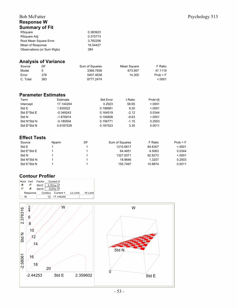
Bob McFatter Psychology 513
- 53 -
Response WSummary of FitRSquare 0.383923RSquare Adj 0.375773Root Mean Square Error 3.782256Mean of Response 16.54427Observations (or Sum Wgts) 384
Analysis of VarianceSource DF Sum of Squares Mean Square F RatioModel 5 3369.7836 673.957 47.1119Error 378 5407.4638 14.305 Prob > FC. Total 383 8777.2474 <.0001
Parameter EstimatesTerm Estimate Std Error t Ratio Prob>|t|Intercept 17.144204 0.2923 58.65 <.0001Std E 1.830522 0.198981 9.20 <.0001Std E*Std E -0.349243 0.164519 -2.12 0.0344Std N -1.876914 0.194808 -9.63 <.0001Std N*Std N -0.180504 0.156771 -1.15 0.2503Std E*Std N 0.6187539 0.187523 3.30 0.0011
Effect TestsSource Nparm DF Sum of Squares F Ratio Prob > FStd E 1 1 1210.6817 84.6307 <.0001Std E*Std E 1 1 64.4651 4.5063 0.0344Std N 1 1 1327.9371 92.8273 <.0001Std N*Std N 1 1 18.9646 1.3257 0.2503Std E*Std N 1 1 155.7497 10.8874 0.0011
Contour ProfilerHoriz Vert
Std EStd N
Factor
3.701e-17-5.67e-17
Current X
W
Response
12
Contour
17.144204
Current Y
.
Lo Limit
.
Hi Limit
2.3
76
31
6S
td N
-2.5
80
61
W
18
16
14
12
10
8
6
42
20
-2.44253 Std E 2.3596020
Std E
Std N
W
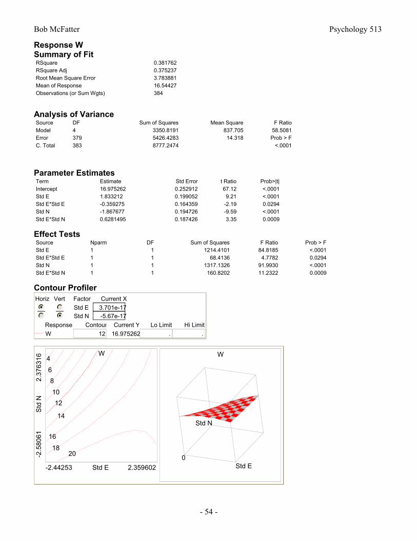
Bob McFatter Psychology 513
- 54 -
Response WSummary of FitRSquare 0.381762RSquare Adj 0.375237Root Mean Square Error 3.783881Mean of Response 16.54427Observations (or Sum Wgts) 384
Analysis of VarianceSource DF Sum of Squares Mean Square F RatioModel 4 3350.8191 837.705 58.5081Error 379 5426.4283 14.318 Prob > FC. Total 383 8777.2474 <.0001
Parameter EstimatesTerm Estimate Std Error t Ratio Prob>|t|Intercept 16.975262 0.252912 67.12 <.0001Std E 1.833212 0.199052 9.21 <.0001Std E*Std E -0.359275 0.164359 -2.19 0.0294Std N -1.867677 0.194726 -9.59 <.0001Std E*Std N 0.6281495 0.187426 3.35 0.0009
Effect TestsSource Nparm DF Sum of Squares F Ratio Prob > FStd E 1 1 1214.4101 84.8185 <.0001Std E*Std E 1 1 68.4136 4.7782 0.0294Std N 1 1 1317.1326 91.9930 <.0001Std E*Std N 1 1 160.8202 11.2322 0.0009
Contour ProfilerHoriz Vert
Std EStd N
Factor
3.701e-17-5.67e-17
Current X
W
Response
12
Contour
16.975262
Current Y
.
Lo Limit
.
Hi Limit
2.3
76
31
6S
td N
-2.5
80
61
W
18
16
14
12
10
8
6
4
20
-2.44253 Std E 2.359602
0Std E
Std N
W

Bob McFatter Psychology 513
- 55 -
Qualitative, Indicator or Dummy Variable Models and ANOVA
The general linear regression model which is given generally by the equation
Yi = β0 + β1 X1i + β2 X2i+ . . . + εi. [57]
may be used to test hypotheses about the means and differences between means of different groups identified by way of variables called qualitative, indicator or dummy variables. These variables code group membership in a numerical code so that the variable may be included in a regression analysis. The most common coding is to use 0 and 1 to encode group membership. Variables that use 0 and 1 in this way are called dummy variables.
In the simplest case, two groups of subjects (e.g., males and females) are coded with one group receiving a 1, the other a 0. If this group dummy variable is correlated with another (criterion) variable, the correlation is often called a point biserial correlation, and a test of H0: ρ = 0 is equivalent to a test of whether the means of the two groups on the criterion variable are equal.
Point-biserial Correlation Example
Subject Score Group Dummy Group1 45 1 Experimental2 52 1 Experimental3 40 1 Experimental4 55 1 Experimental5 43 1 Experimental6 44 1 Experimental7 48 1 Experimental8 37 1 Experimental9 44 1 Experimental
10 56 0 Control11 54 0 Control12 61 0 Control13 48 0 Control14 57 0 Control15 50 0 Control16 56 0 Control17 55 0 Control18 47 0 Control19 60 0 Control
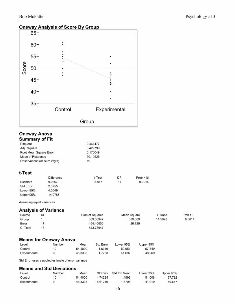
Bob McFatter Psychology 513
- 56 -
Oneway Analysis of Score By GroupS
core
35
40
45
50
55
60
65
Control Experimental
Group
Oneway AnovaSummary of FitRsquare 0.461477Adj Rsquare 0.429799Root Mean Square Error 5.170049Mean of Response 50.10526Observations (or Sum Wgts) 19
t-TestDifference t-Test DF Prob > |t|
Estimate 9.0667 3.817 17 0.0014Std Error 2.3755Lower 95% 4.0549Upper 95% 14.0785
Assuming equal variances
Analysis of VarianceSource DF Sum of Squares Mean Square F Ratio Prob > FGroup 1 389.38947 389.389 14.5678 0.0014Error 17 454.40000 26.729C. Total 18 843.78947
Means for Oneway AnovaLevel Number Mean Std Error Lower 95% Upper 95%Control 10 54.4000 1.6349 50.951 57.849Experimental 9 45.3333 1.7233 41.697 48.969
Std Error uses a pooled estimate of error variance
Means and Std DeviationsLevel Number Mean Std Dev Std Err Mean Lower 95% Upper 95%Control 10 54.4000 4.74225 1.4996 51.008 57.792Experimental 9 45.3333 5.61249 1.8708 41.019 49.647

Bob McFatter Psychology 513
- 57 -
Multivariate Correlations
Score Group DummyScore 1.0000 -0.6793Group Dummy -0.6793 1.0000
Pairwise CorrelationsVariable by Variable Correlation Count Signif ProbGroup Dummy Score -0.6793 19 0.0014 ----------------------------
Bivariate Fit of Score By Group Dummy
35
40
45
50
55
60
65
Sco
re
-0.25 0 .25 .5 .75 1 1.25
Group Dummy
Linear FitLinear FitScore = 54.4 - 9.0666667 Group Dummy
Summary of FitRSquare 0.461477RSquare Adj 0.429799Root Mean Square Error 5.170049Mean of Response 50.10526Observations (or Sum Wgts) 19
Analysis of VarianceSource DF Sum of Squares Mean Square F RatioModel 1 389.38947 389.389 14.5678Error 17 454.40000 26.729 Prob > FC. Total 18 843.78947 0.0014
Parameter EstimatesTerm Estimate Std Error t Ratio Prob>|t|Intercept 54.4 1.634913 33.27 <.0001Group Dummy -9.066667 2.375474 -3.82 0.0014

Bob McFatter Psychology 513
- 58 -
Example for different coding methods
Assume we have scores on 3 subjects in each of 4 groups:
a1 a2 a3 a4
2 9 5 94 6 5 83 3 2 4
We may code group membership in several ways as shown in the table below. The first set of three predictors is ‘dummy coding,’ the second is ‘effects coding,’ the third ‘Helmert coding,’ the fourth ‘effects coding’ for a two way factorial ANOVA, and the last columns just use index numbers to indicate group membership.
Perf D1 D2 D3 E1 E2 E3 H1 H2 H3 A B A×B Betw FacA FacB2 1 0 0 1 0 0 3 0 0 1 1 1 1 1 14 1 0 0 1 0 0 3 0 0 1 1 1 1 1 13 1 0 0 1 0 0 3 0 0 1 1 1 1 1 19 0 1 0 0 1 0 -1 2 0 1 -1 -1 2 1 26 0 1 0 0 1 0 -1 2 0 1 -1 -1 2 1 23 0 1 0 0 1 0 -1 2 0 1 -1 -1 2 1 25 0 0 1 0 0 1 -1 -1 1 -1 1 -1 3 2 15 0 0 1 0 0 1 -1 -1 1 -1 1 -1 3 2 12 0 0 1 0 0 1 -1 -1 1 -1 1 -1 3 2 19 0 0 0 -1 -1 -1 -1 -1 -1 -1 -1 1 4 2 28 0 0 0 -1 -1 -1 -1 -1 -1 -1 -1 1 4 2 24 0 0 0 -1 -1 -1 -1 -1 -1 -1 -1 1 4 2 2

Bob McFatter Psychology 513
- 59 -
1 Example for various coding methods 1 General Linear Models Procedure Number of observations in data set = 12
Dummy Coding 2
General Linear Models Procedure
Dependent Variable: PERF Sum of Mean Source DF Squares Square F Value Pr > F
Model 3 30.000000 10.000000 2.00 0.1927 Error 8 40.000000 5.000000 Corrected Total 11 70.000000
R-Square C.V. Root MSE PERF Mean 0.428571 44.72136 2.2361 5.0000
Source DF Type I SS Mean Square F Value Pr > F D1 1 16.000000 16.000000 3.20 0.1114 D2 1 0.500000 0.500000 0.10 0.7599 D3 1 13.500000 13.500000 2.70 0.1390
Source DF Type III SS Mean Square F Value Pr > F D1 1 24.000000 24.000000 4.80 0.0598 D2 1 1.500000 1.500000 0.30 0.5988 D3 1 13.500000 13.500000 2.70 0.1390
T for H0: Pr > |T| Std Error of Parameter Estimate Parameter=0 Estimate INTERCEPT 7.000000000 5.42 0.0006 1.29099445 D1 -4.000000000 -2.19 0.0598 1.82574186 D2 -1.000000000 -0.55 0.5988 1.82574186 D3 -3.000000000 -1.64 0.1390 1.82574186
Effects Coding 3 General Linear Models Procedure Number of observations in data set = 12 This is effects coding 4 General Linear Models Procedure
Dependent Variable: PERF Sum of Mean Source DF Squares Square F Value Pr > F Model 3 30.000000 10.000000 2.00 0.1927 Error 8 40.000000 5.000000 Corrected Total 11 70.000000
R-Square C.V. Root MSE PERF Mean 0.428571 44.72136 2.2361 5.0000
Source DF Type I SS Mean Square F Value Pr > F E1 1 24.000000 24.000000 4.80 0.0598 E2 1 2.000000 2.000000 0.40 0.5447 E3 1 4.000000 4.000000 0.80 0.3972
Source DF Type III SS Mean Square F Value Pr > F E1 1 16.000000 16.000000 3.20 0.1114 E2 1 4.000000 4.000000 0.80 0.3972 E3 1 4.000000 4.000000 0.80 0.3972
T for H0: Pr > |T| Std Error of Parameter Estimate Parameter=0 Estimate INTERCEPT 5.000000000 7.75 0.0001 0.64549722 E1 -2.000000000 -1.79 0.1114 1.11803399 E2 1.000000000 0.89 0.3972 1.11803399 E3 -1.000000000 -0.89 0.3972 1.11803399

Bob McFatter Psychology 513
- 60 -
Helmert Contrast Coding 5 General Linear Models Procedure Number of observations in data set = 12 This is helmert contrast coding 6 General Linear Models Procedure
Dependent Variable: PERF Sum of Mean Source DF Squares Square F Value Pr > F Model 3 30.000000 10.000000 2.00 0.1927 Error 8 40.000000 5.000000
Corrected Total 11 70.000000
R-Square C.V. Root MSE PERF Mean 0.428571 44.72136 2.2361 5.0000
Source DF Type I SS Mean Square F Value Pr > F H1 1 16.000000 16.000000 3.20 0.1114 H2 1 0.500000 0.500000 0.10 0.7599 H3 1 13.500000 13.500000 2.70 0.1390
Source DF Type III SS Mean Square F Value Pr > F H1 1 16.000000 16.000000 3.20 0.1114 H2 1 0.500000 0.500000 0.10 0.7599 H3 1 13.500000 13.500000 2.70 0.1390
T for H0: Pr > |T| Std Error of Parameter Estimate Parameter=0 Estimate INTERCEPT 5.000000000 7.75 0.0001 0.64549722 H1 -0.666666667 -1.79 0.1114 0.37267800 H2 0.166666667 0.32 0.7599 0.52704628 H3 -1.500000000 -1.64 0.1390 0.91287093
2×2 Factorial Design Effects Coding 7 General Linear Models Procedure Number of observations in data set = 12 This is a 2×2 factorial design coding 8 General Linear Models Procedure
Dependent Variable: PERF Sum of Mean Source DF Squares Square F Value Pr > F Model 3 30.000000 10.000000 2.00 0.1927 Error 8 40.000000 5.000000 Corrected Total 11 70.000000
R-Square C.V. Root MSE PERF Mean 0.428571 44.72136 2.2361 5.0000
Source DF Type I SS Mean Square F Value Pr > F A 1 3.000000 3.000000 0.60 0.4609 B 1 27.000000 27.000000 5.40 0.0486 AXB 1 0.000000 0.000000 0.00 1.0000
Source DF Type III SS Mean Square F Value Pr > F A 1 3.000000 3.000000 0.60 0.4609 B 1 27.000000 27.000000 5.40 0.0486 AXB 1 0.000000 0.000000 0.00 1.0000
T for H0: Pr > |T| Std Error of Parameter Estimate Parameter=0 Estimate INTERCEPT 5.000000000 7.75 0.0001 0.64549722 A -0.500000000 -0.77 0.4609 0.64549722 B -1.500000000 -2.32 0.0486 0.64549722 AXB 0.000000000 0.00 1.0000 0.64549722
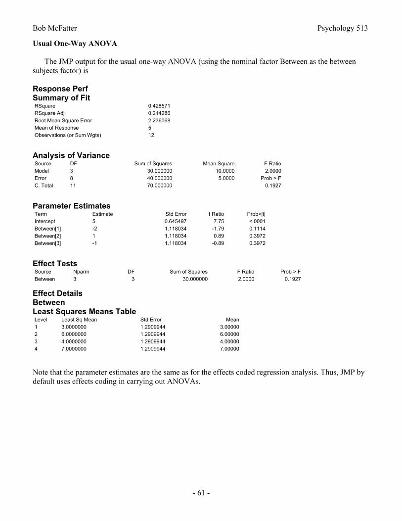
Bob McFatter Psychology 513
- 61 -
Usual One-Way ANOVA
The JMP output for the usual one-way ANOVA (using the nominal factor Between as the between subjects factor) is
Response PerfSummary of FitRSquare 0.428571RSquare Adj 0.214286Root Mean Square Error 2.236068Mean of Response 5Observations (or Sum Wgts) 12
Analysis of VarianceSource DF Sum of Squares Mean Square F RatioModel 3 30.000000 10.0000 2.0000Error 8 40.000000 5.0000 Prob > FC. Total 11 70.000000 0.1927
Parameter EstimatesTerm Estimate Std Error t Ratio Prob>|t|Intercept 5 0.645497 7.75 <.0001Between[1] -2 1.118034 -1.79 0.1114Between[2] 1 1.118034 0.89 0.3972Between[3] -1 1.118034 -0.89 0.3972
Effect TestsSource Nparm DF Sum of Squares F Ratio Prob > FBetween 3 3 30.000000 2.0000 0.1927
Effect DetailsBetweenLeast Squares Means TableLevel Least Sq Mean Std Error Mean1 3.0000000 1.2909944 3.000002 6.0000000 1.2909944 6.000003 4.0000000 1.2909944 4.000004 7.0000000 1.2909944 7.00000
Note that the parameter estimates are the same as for the effects coded regression analysis. Thus, JMP by default uses effects coding in carrying out ANOVAs.
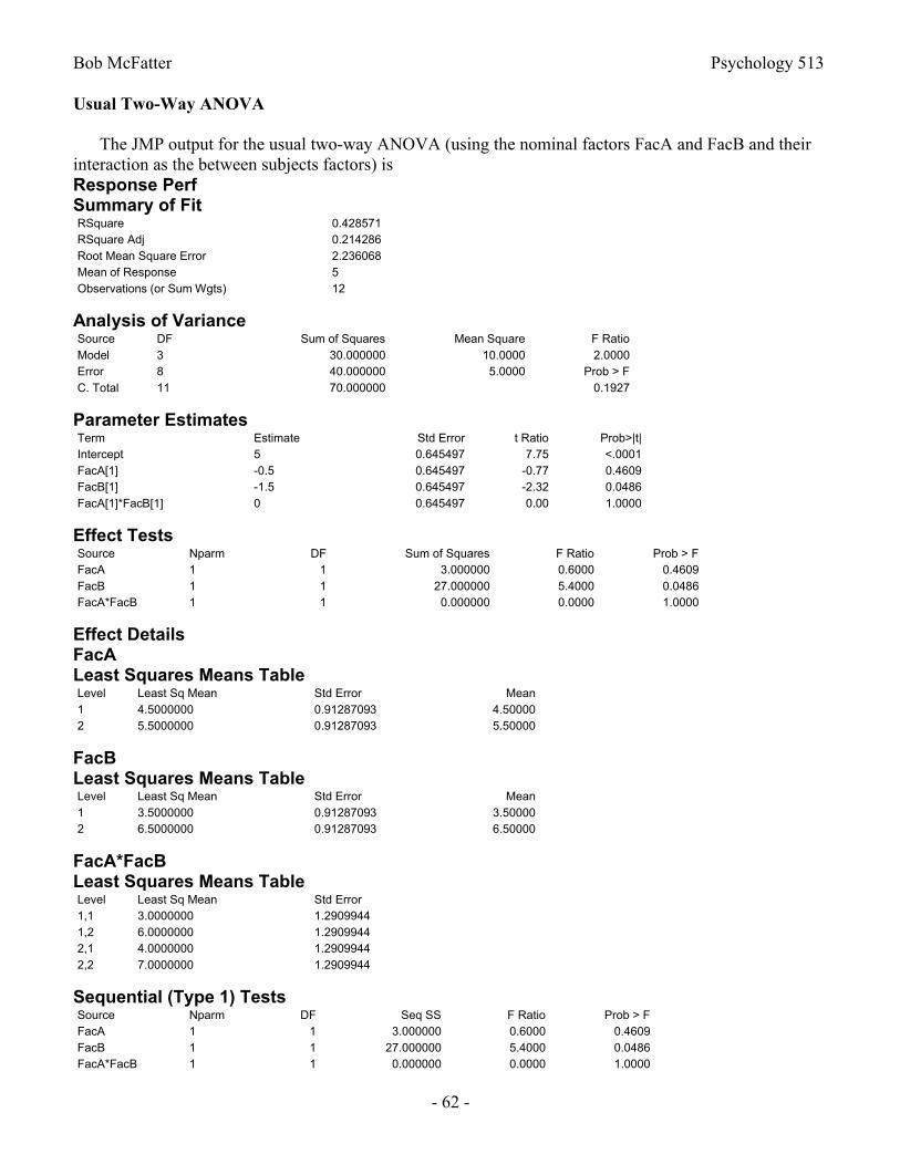
Bob McFatter Psychology 513
- 62 -
Usual Two-Way ANOVA
The JMP output for the usual two-way ANOVA (using the nominal factors FacA and FacB and their interaction as the between subjects factors) isResponse PerfSummary of FitRSquare 0.428571RSquare Adj 0.214286Root Mean Square Error 2.236068Mean of Response 5Observations (or Sum Wgts) 12
Analysis of VarianceSource DF Sum of Squares Mean Square F RatioModel 3 30.000000 10.0000 2.0000Error 8 40.000000 5.0000 Prob > FC. Total 11 70.000000 0.1927
Parameter EstimatesTerm Estimate Std Error t Ratio Prob>|t|Intercept 5 0.645497 7.75 <.0001FacA[1] -0.5 0.645497 -0.77 0.4609FacB[1] -1.5 0.645497 -2.32 0.0486FacA[1]*FacB[1] 0 0.645497 0.00 1.0000
Effect TestsSource Nparm DF Sum of Squares F Ratio Prob > FFacA 1 1 3.000000 0.6000 0.4609FacB 1 1 27.000000 5.4000 0.0486FacA*FacB 1 1 0.000000 0.0000 1.0000
Effect DetailsFacALeast Squares Means TableLevel Least Sq Mean Std Error Mean1 4.5000000 0.91287093 4.500002 5.5000000 0.91287093 5.50000
FacBLeast Squares Means TableLevel Least Sq Mean Std Error Mean1 3.5000000 0.91287093 3.500002 6.5000000 0.91287093 6.50000
FacA*FacBLeast Squares Means TableLevel Least Sq Mean Std Error1,1 3.0000000 1.29099441,2 6.0000000 1.29099442,1 4.0000000 1.29099442,2 7.0000000 1.2909944
Sequential (Type 1) TestsSource Nparm DF Seq SS F Ratio Prob > FFacA 1 1 3.000000 0.6000 0.4609FacB 1 1 27.000000 5.4000 0.0486FacA*FacB 1 1 0.000000 0.0000 1.0000
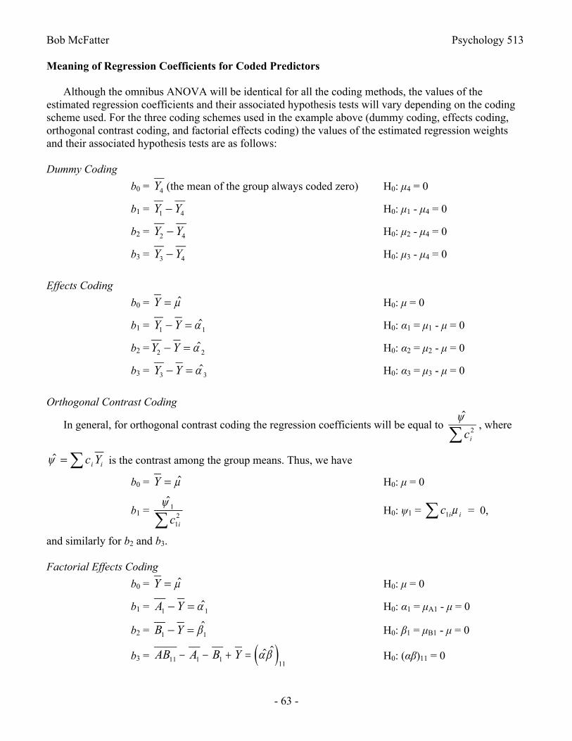
Bob McFatter Psychology 513
- 63 -
Meaning of Regression Coefficients for Coded Predictors
Although the omnibus ANOVA will be identical for all the coding methods, the values of the estimated regression coefficients and their associated hypothesis tests will vary depending on the coding scheme used. For the three coding schemes used in the example above (dummy coding, effects coding, orthogonal contrast coding, and factorial effects coding) the values of the estimated regression weights and their associated hypothesis tests are as follows:
Dummy Coding
b0 = Y4 (the mean of the group always coded zero) H0: μ4 = 0
b1 = Y Y1 4 H0: μ1 - μ4 = 0
b2 = Y Y2 4 H0: μ2 - μ4 = 0
b3 = Y Y3 4 H0: μ3 - μ4 = 0
Effects Coding
b0 = Y H0: μ = 0
b1 = Y Y1 1 H0: α1 = μ1 - μ = 0
b2 = Y Y2 2 H0: α2 = μ2 - μ = 0
b3 = Y Y3 3 H0: α3 = μ3 - μ = 0
Orthogonal Contrast Coding
In general, for orthogonal contrast coding the regression coefficients will be equal to ci
2, where
c Yi i is the contrast among the group means. Thus, we have
b0 = Y H0: μ = 0
b1 = 1
12c i
H0: ψ1 = c i i1 = 0,
and similarly for b2 and b3.
Factorial Effects Coding
b0 = Y H0: μ = 0
b1 = A Y1 1 H0: α1 = μA1 - μ = 0
b2 = B Y1 1 H0: β1 = μB1 - μ = 0
b3 = AB A B Y11 1 111
H0: (αβ)11 = 0
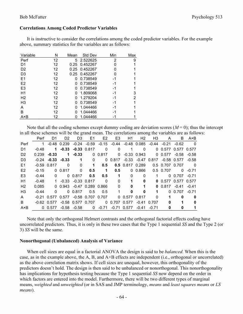
Bob McFatter Psychology 513
- 64 -
Correlations Among Coded Predictor Variables
It is instructive to consider the correlations among the coded predictor variables. For the example above, summary statistics for the variables are as follows:
Variable N Mean Std Dev Min MaxPerf 12 5 2.522625 2 9D1 12 0.25 0.452267 0 1D2 12 0.25 0.452267 0 1D3 12 0.25 0.452267 0 1E1 12 0 0.738549 -1 1E2 12 0 0.738549 -1 1E3 12 0 0.738549 -1 1H1 12 0 1.809068 -1 3H2 12 0 1.279204 -1 2H3 12 0 0.738549 -1 1A 12 0 1.044466 -1 1B 12 0 1.044466 -1 1A×B 12 0 1.044466 -1 1
Note that all the coding schemes except dummy coding are deviation scores (M = 0); thus the intercept in all these schemes will be the grand mean. The correlations among the variables are as follows:
Perf D1 D2 D3 E1 E2 E3 H1 H2 H3 A B A×B
Perf 1 -0.48 0.239 -0.24 -0.59 -0.15 -0.44 -0.48 0.085 -0.44 -0.21 -0.62 0D1 -0.48 1 -0.33 -0.33 0.817 0 0 1 0 0 0.577 0.577 0.577D2 0.239 -0.33 1 -0.33 0 0.817 0 -0.33 0.943 0 0.577 -0.58 -0.58D3 -0.24 -0.33 -0.33 1 0 0 0.817 -0.33 -0.47 0.817 -0.58 0.577 -0.58E1 -0.59 0.817 0 0 1 0.5 0.5 0.817 0.289 0.5 0.707 0.707 0E2 -0.15 0 0.817 0 0.5 1 0.5 0 0.866 0.5 0.707 0 -0.71E3 -0.44 0 0 0.817 0.5 0.5 1 0 0 1 0 0.707 -0.71H1 -0.48 1 -0.33 -0.33 0.817 0 0 1 0 0 0.577 0.577 0.577H2 0.085 0 0.943 -0.47 0.289 0.866 0 0 1 0 0.817 -0.41 -0.41H3 -0.44 0 0 0.817 0.5 0.5 1 0 0 1 0 0.707 -0.71A -0.21 0.577 0.577 -0.58 0.707 0.707 0 0.577 0.817 0 1 0 0B -0.62 0.577 -0.58 0.577 0.707 0 0.707 0.577 -0.41 0.707 0 1 0A×B 0 0.577 -0.58 -0.58 0 -0.71 -0.71 0.577 -0.41 -0.71 0 0 1
Note that only the orthogonal Helmert contrasts and the orthogonal factorial effects coding have uncorrelated predictors. Thus, it is only in these two cases that the Type 1 sequential SS and the Type 2 (or 3) SS will be the same.
Nonorthogonal (Unbalanced) Analysis of Variance
When cell sizes are equal in a factorial ANOVA the design is said to be balanced. When this is the case, as in the example above, the A, B, and A×B effects are independent (i.e., orthogonal or uncorrelated) as the above correlation matrix shows. If cell sizes are unequal, however, this orthogonality of the predictors doesn’t hold. The design is then said to be unbalanced or nonorthogonal. This nonorthogonality has implications for hypothesis testing because the Type 1 sequential SS now depend on the order in which factors are entered into the model. Furthermore, there will be two different types of marginal means, weighted and unweighted (or in SAS and JMP terminology, means and least squares means or LS means).
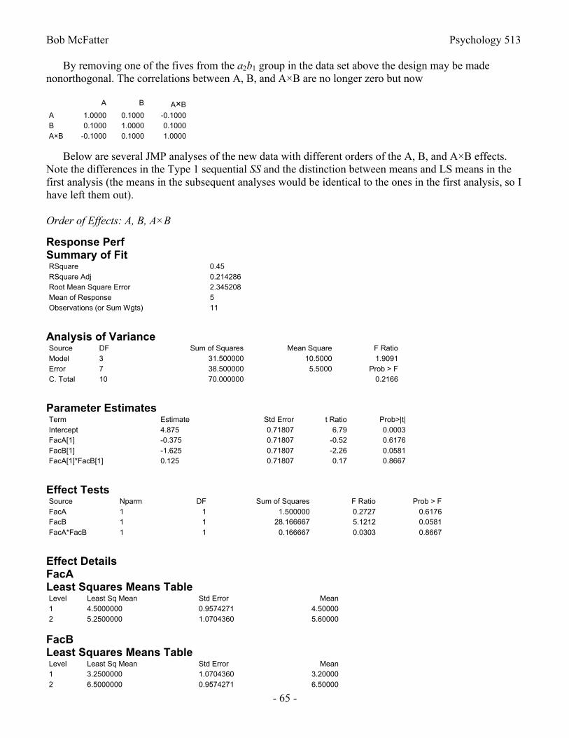
Bob McFatter Psychology 513
- 65 -
By removing one of the fives from the a2b1 group in the data set above the design may be made nonorthogonal. The correlations between A, B, and A×B are no longer zero but now
A B A×B
A 1.0000 0.1000 -0.1000B 0.1000 1.0000 0.1000A×B -0.1000 0.1000 1.0000
Below are several JMP analyses of the new data with different orders of the A, B, and A×B effects. Note the differences in the Type 1 sequential SS and the distinction between means and LS means in the first analysis (the means in the subsequent analyses would be identical to the ones in the first analysis, so I have left them out).
Order of Effects: A, B, A×B
Response PerfSummary of FitRSquare 0.45RSquare Adj 0.214286Root Mean Square Error 2.345208Mean of Response 5Observations (or Sum Wgts) 11
Analysis of VarianceSource DF Sum of Squares Mean Square F RatioModel 3 31.500000 10.5000 1.9091Error 7 38.500000 5.5000 Prob > FC. Total 10 70.000000 0.2166
Parameter EstimatesTerm Estimate Std Error t Ratio Prob>|t|Intercept 4.875 0.71807 6.79 0.0003FacA[1] -0.375 0.71807 -0.52 0.6176FacB[1] -1.625 0.71807 -2.26 0.0581FacA[1]*FacB[1] 0.125 0.71807 0.17 0.8667
Effect TestsSource Nparm DF Sum of Squares F Ratio Prob > FFacA 1 1 1.500000 0.2727 0.6176FacB 1 1 28.166667 5.1212 0.0581FacA*FacB 1 1 0.166667 0.0303 0.8667
Effect DetailsFacALeast Squares Means TableLevel Least Sq Mean Std Error Mean1 4.5000000 0.9574271 4.500002 5.2500000 1.0704360 5.60000
FacBLeast Squares Means TableLevel Least Sq Mean Std Error Mean1 3.2500000 1.0704360 3.200002 6.5000000 0.9574271 6.50000

Bob McFatter Psychology 513
- 66 -
FacA*FacBLeast Squares Means TableLevel Least Sq Mean Std Error1,1 3.0000000 1.35400641,2 6.0000000 1.35400642,1 3.5000000 1.65831242,2 7.0000000 1.3540064
Sequential (Type 1) TestsSource Nparm DF Seq SS F Ratio Prob > FFacA 1 1 3.300000 0.6000 0.4639FacB 1 1 28.033333 5.0970 0.0585FacA*FacB 1 1 0.166667 0.0303 0.8667
Order of Effects: B, A, A×B
Response PerfSummary of FitRSquare 0.45RSquare Adj 0.214286Root Mean Square Error 2.345208Mean of Response 5Observations (or Sum Wgts) 11
Analysis of VarianceSource DF Sum of Squares Mean Square F RatioModel 3 31.500000 10.5000 1.9091Error 7 38.500000 5.5000 Prob > FC. Total 10 70.000000 0.2166
Parameter EstimatesTerm Estimate Std Error t Ratio Prob>|t|Intercept 4.875 0.71807 6.79 0.0003FacB[1] -1.625 0.71807 -2.26 0.0581FacA[1] -0.375 0.71807 -0.52 0.6176FacA[1]*FacB[1] 0.125 0.71807 0.17 0.8667
Effect TestsSource Nparm DF Sum of Squares F Ratio Prob > FFacB 1 1 28.166667 5.1212 0.0581FacA 1 1 1.500000 0.2727 0.6176FacA*FacB 1 1 0.166667 0.0303 0.8667
Sequential (Type 1) TestsSource Nparm DF Seq SS F Ratio Prob > FFacB 1 1 29.700000 5.4000 0.0531FacA 1 1 1.633333 0.2970 0.6027FacA*FacB 1 1 0.166667 0.0303 0.8667
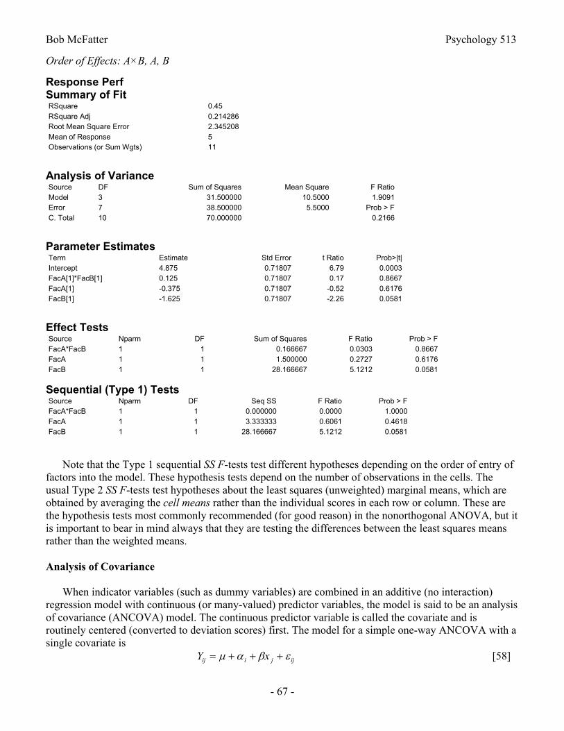
Bob McFatter Psychology 513
- 67 -
Order of Effects: A×B, A, B
Response PerfSummary of FitRSquare 0.45RSquare Adj 0.214286Root Mean Square Error 2.345208Mean of Response 5Observations (or Sum Wgts) 11
Analysis of VarianceSource DF Sum of Squares Mean Square F RatioModel 3 31.500000 10.5000 1.9091Error 7 38.500000 5.5000 Prob > FC. Total 10 70.000000 0.2166
Parameter EstimatesTerm Estimate Std Error t Ratio Prob>|t|Intercept 4.875 0.71807 6.79 0.0003FacA[1]*FacB[1] 0.125 0.71807 0.17 0.8667FacA[1] -0.375 0.71807 -0.52 0.6176FacB[1] -1.625 0.71807 -2.26 0.0581
Effect TestsSource Nparm DF Sum of Squares F Ratio Prob > FFacA*FacB 1 1 0.166667 0.0303 0.8667FacA 1 1 1.500000 0.2727 0.6176FacB 1 1 28.166667 5.1212 0.0581
Sequential (Type 1) TestsSource Nparm DF Seq SS F Ratio Prob > FFacA*FacB 1 1 0.000000 0.0000 1.0000FacA 1 1 3.333333 0.6061 0.4618FacB 1 1 28.166667 5.1212 0.0581
Note that the Type 1 sequential SS F-tests test different hypotheses depending on the order of entry of factors into the model. These hypothesis tests depend on the number of observations in the cells. The usual Type 2 SS F-tests test hypotheses about the least squares (unweighted) marginal means, which are obtained by averaging the cell means rather than the individual scores in each row or column. These are the hypothesis tests most commonly recommended (for good reason) in the nonorthogonal ANOVA, but it is important to bear in mind always that they are testing the differences between the least squares means rather than the weighted means.
Analysis of Covariance
When indicator variables (such as dummy variables) are combined in an additive (no interaction) regression model with continuous (or many-valued) predictor variables, the model is said to be an analysis of covariance (ANCOVA) model. The continuous predictor variable is called the covariate and is routinely centered (converted to deviation scores) first. The model for a simple one-way ANCOVA with a single covariate is
Y xij i j ij [58]
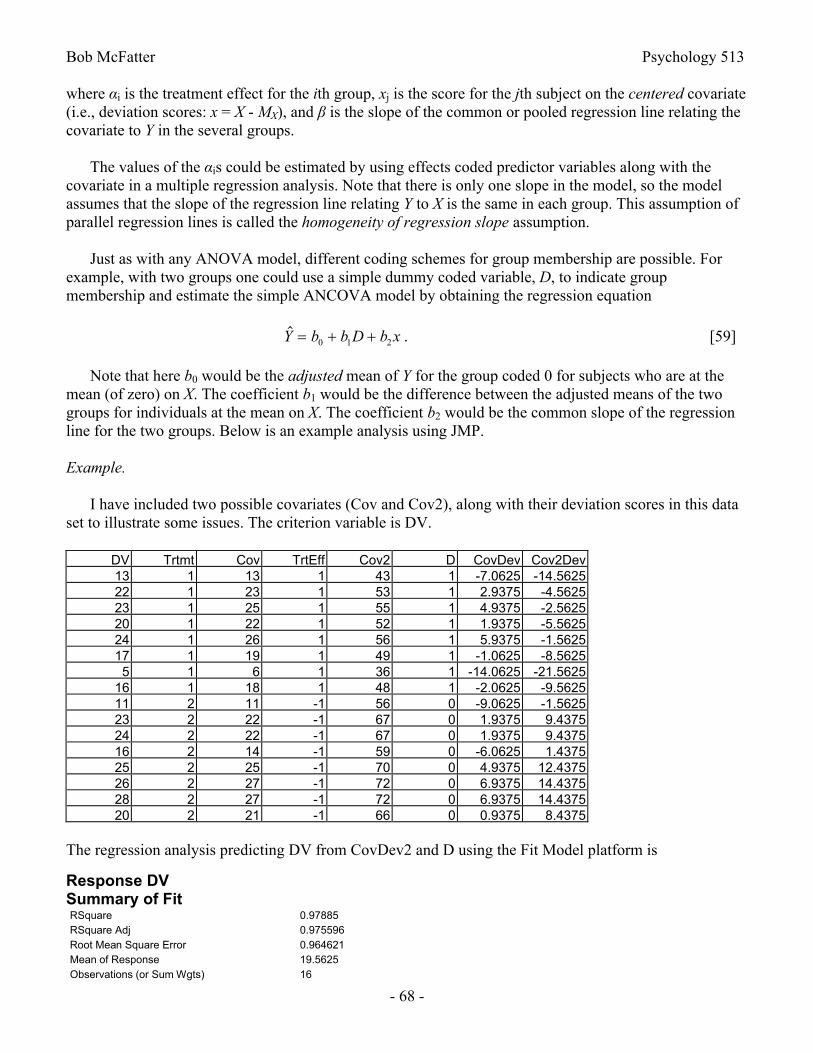
Bob McFatter Psychology 513
- 68 -
where αi is the treatment effect for the ith group, xj is the score for the jth subject on the centered covariate (i.e., deviation scores: x = X - MX), and β is the slope of the common or pooled regression line relating the covariate to Y in the several groups.
The values of the αis could be estimated by using effects coded predictor variables along with the covariate in a multiple regression analysis. Note that there is only one slope in the model, so the model assumes that the slope of the regression line relating Y to X is the same in each group. This assumption of parallel regression lines is called the homogeneity of regression slope assumption.
Just as with any ANOVA model, different coding schemes for group membership are possible. For example, with two groups one could use a simple dummy coded variable, D, to indicate group membership and estimate the simple ANCOVA model by obtaining the regression equation
Y b b D b x 0 1 2 . [59]
Note that here b0 would be the adjusted mean of Y for the group coded 0 for subjects who are at the mean (of zero) on X. The coefficient b1 would be the difference between the adjusted means of the two groups for individuals at the mean on X. The coefficient b2 would be the common slope of the regression line for the two groups. Below is an example analysis using JMP.
Example.
I have included two possible covariates (Cov and Cov2), along with their deviation scores in this data set to illustrate some issues. The criterion variable is DV.
DV Trtmt Cov TrtEff Cov2 D CovDev Cov2Dev13 1 13 1 43 1 -7.0625 -14.562522 1 23 1 53 1 2.9375 -4.562523 1 25 1 55 1 4.9375 -2.562520 1 22 1 52 1 1.9375 -5.562524 1 26 1 56 1 5.9375 -1.562517 1 19 1 49 1 -1.0625 -8.56255 1 6 1 36 1 -14.0625 -21.5625
16 1 18 1 48 1 -2.0625 -9.562511 2 11 -1 56 0 -9.0625 -1.562523 2 22 -1 67 0 1.9375 9.437524 2 22 -1 67 0 1.9375 9.437516 2 14 -1 59 0 -6.0625 1.437525 2 25 -1 70 0 4.9375 12.437526 2 27 -1 72 0 6.9375 14.437528 2 27 -1 72 0 6.9375 14.437520 2 21 -1 66 0 0.9375 8.4375
The regression analysis predicting DV from CovDev2 and D using the Fit Model platform is
Response DVSummary of FitRSquare 0.97885RSquare Adj 0.975596Root Mean Square Error 0.964621Mean of Response 19.5625Observations (or Sum Wgts) 16
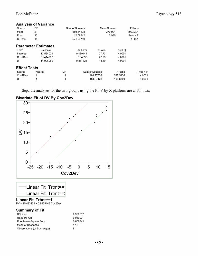
Bob McFatter Psychology 513
- 69 -
Analysis of VarianceSource DF Sum of Squares Mean Square F RatioModel 2 559.84108 279.921 300.8301Error 13 12.09642 0.930 Prob > FC. Total 15 571.93750 <.0001
Parameter EstimatesTerm Estimate Std Error t Ratio Prob>|t|Intercept 13.564021 0.489141 27.73 <.0001Cov2Dev 0.9414282 0.04095 22.99 <.0001D 11.996959 0.851125 14.10 <.0001
Effect TestsSource Nparm DF Sum of Squares F Ratio Prob > FCov2Dev 1 1 491.77858 528.5136 <.0001D 1 1 184.87128 198.6809 <.0001
Separate analyses for the two groups using the Fit Y by X platform are as follows:
Bivariate Fit of DV By Cov2Dev
0
5
10
15
20
25
30
DV
-25 -20 -15 -10 -5 0 5 10 15
Cov2Dev
Linear Fit Trtmt==1Linear Fit Trtmt==2
Linear Fit Trtmt==1DV = 25.493473 + 0.9335443 Cov2Dev
Summary of FitRSquare 0.990632RSquare Adj 0.98907Root Mean Square Error 0.658841Mean of Response 17.5Observations (or Sum Wgts) 8
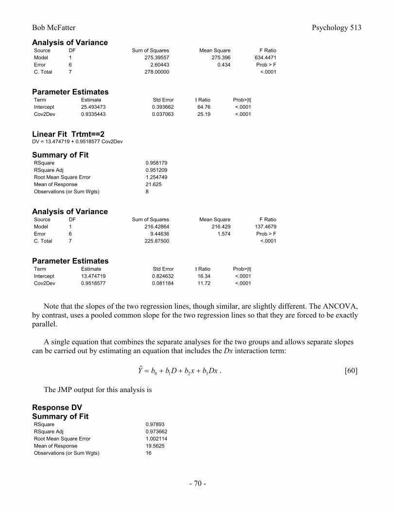
Bob McFatter Psychology 513
- 70 -
Analysis of VarianceSource DF Sum of Squares Mean Square F RatioModel 1 275.39557 275.396 634.4471Error 6 2.60443 0.434 Prob > FC. Total 7 278.00000 <.0001
Parameter EstimatesTerm Estimate Std Error t Ratio Prob>|t|Intercept 25.493473 0.393662 64.76 <.0001Cov2Dev 0.9335443 0.037063 25.19 <.0001
Linear Fit Trtmt==2DV = 13.474719 + 0.9518577 Cov2Dev
Summary of FitRSquare 0.958179RSquare Adj 0.951209Root Mean Square Error 1.254749Mean of Response 21.625Observations (or Sum Wgts) 8
Analysis of VarianceSource DF Sum of Squares Mean Square F RatioModel 1 216.42864 216.429 137.4679Error 6 9.44636 1.574 Prob > FC. Total 7 225.87500 <.0001
Parameter EstimatesTerm Estimate Std Error t Ratio Prob>|t|Intercept 13.474719 0.824632 16.34 <.0001Cov2Dev 0.9518577 0.081184 11.72 <.0001
Note that the slopes of the two regression lines, though similar, are slightly different. The ANCOVA, by contrast, uses a pooled common slope for the two regression lines so that they are forced to be exactly parallel.
A single equation that combines the separate analyses for the two groups and allows separate slopes can be carried out by estimating an equation that includes the Dx interaction term:
Y b b D b x b Dx 0 1 2 3 . [60]
The JMP output for this analysis is
Response DVSummary of FitRSquare 0.97893RSquare Adj 0.973662Root Mean Square Error 1.002114Mean of Response 19.5625Observations (or Sum Wgts) 16
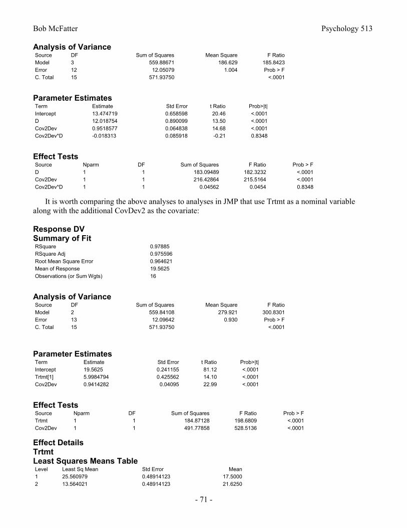
Bob McFatter Psychology 513
- 71 -
Analysis of VarianceSource DF Sum of Squares Mean Square F RatioModel 3 559.88671 186.629 185.8423Error 12 12.05079 1.004 Prob > FC. Total 15 571.93750 <.0001
Parameter EstimatesTerm Estimate Std Error t Ratio Prob>|t|Intercept 13.474719 0.658598 20.46 <.0001D 12.018754 0.890099 13.50 <.0001Cov2Dev 0.9518577 0.064838 14.68 <.0001Cov2Dev*D -0.018313 0.085918 -0.21 0.8348
Effect TestsSource Nparm DF Sum of Squares F Ratio Prob > FD 1 1 183.09489 182.3232 <.0001Cov2Dev 1 1 216.42864 215.5164 <.0001Cov2Dev*D 1 1 0.04562 0.0454 0.8348
It is worth comparing the above analyses to analyses in JMP that use Trtmt as a nominal variable along with the additional CovDev2 as the covariate:
Response DVSummary of FitRSquare 0.97885RSquare Adj 0.975596Root Mean Square Error 0.964621Mean of Response 19.5625Observations (or Sum Wgts) 16
Analysis of VarianceSource DF Sum of Squares Mean Square F RatioModel 2 559.84108 279.921 300.8301Error 13 12.09642 0.930 Prob > FC. Total 15 571.93750 <.0001
Parameter EstimatesTerm Estimate Std Error t Ratio Prob>|t|Intercept 19.5625 0.241155 81.12 <.0001Trtmt[1] 5.9984794 0.425562 14.10 <.0001Cov2Dev 0.9414282 0.04095 22.99 <.0001
Effect TestsSource Nparm DF Sum of Squares F Ratio Prob > FTrtmt 1 1 184.87128 198.6809 <.0001Cov2Dev 1 1 491.77858 528.5136 <.0001
Effect DetailsTrtmtLeast Squares Means TableLevel Least Sq Mean Std Error Mean1 25.560979 0.48914123 17.50002 13.564021 0.48914123 21.6250
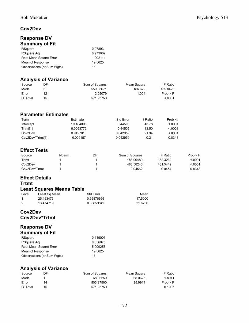
Bob McFatter Psychology 513
- 72 -
Cov2Dev
Response DVSummary of FitRSquare 0.97893RSquare Adj 0.973662Root Mean Square Error 1.002114Mean of Response 19.5625Observations (or Sum Wgts) 16
Analysis of VarianceSource DF Sum of Squares Mean Square F RatioModel 3 559.88671 186.629 185.8423Error 12 12.05079 1.004 Prob > FC. Total 15 571.93750 <.0001
Parameter EstimatesTerm Estimate Std Error t Ratio Prob>|t|Intercept 19.484096 0.44505 43.78 <.0001Trtmt[1] 6.0093772 0.44505 13.50 <.0001Cov2Dev 0.942701 0.042959 21.94 <.0001Cov2Dev*Trtmt[1] -0.009157 0.042959 -0.21 0.8348
Effect TestsSource Nparm DF Sum of Squares F Ratio Prob > FTrtmt 1 1 183.09489 182.3232 <.0001Cov2Dev 1 1 483.58246 481.5442 <.0001Cov2Dev*Trtmt 1 1 0.04562 0.0454 0.8348
Effect DetailsTrtmtLeast Squares Means TableLevel Least Sq Mean Std Error Mean1 25.493473 0.59876966 17.50002 13.474719 0.65859849 21.6250
Cov2DevCov2Dev*Trtmt
Response DVSummary of FitRSquare 0.119003RSquare Adj 0.056075Root Mean Square Error 5.999256Mean of Response 19.5625Observations (or Sum Wgts) 16
Analysis of VarianceSource DF Sum of Squares Mean Square F RatioModel 1 68.06250 68.0625 1.8911Error 14 503.87500 35.9911 Prob > FC. Total 15 571.93750 0.1907
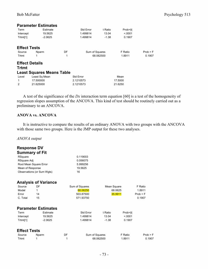
Bob McFatter Psychology 513
- 73 -
Parameter EstimatesTerm Estimate Std Error t Ratio Prob>|t|Intercept 19.5625 1.499814 13.04 <.0001Trtmt[1] -2.0625 1.499814 -1.38 0.1907
Effect TestsSource Nparm DF Sum of Squares F Ratio Prob > FTrtmt 1 1 68.062500 1.8911 0.1907
Effect DetailsTrtmtLeast Squares Means TableLevel Least Sq Mean Std Error Mean1 17.500000 2.1210573 17.50002 21.625000 2.1210573 21.6250
A test of the significance of the Dx interaction term equation [60] is a test of the homogeneity of regression slopes assumption of the ANCOVA. This kind of test should be routinely carried out as a preliminary to an ANCOVA.
ANOVA vs. ANCOVA
It is instructive to compare the results of an ordinary ANOVA with two groups with the ANCOVA with those same two groups. Here is the JMP output for these two analyses.
ANOVA output
Response DVSummary of FitRSquare 0.119003RSquare Adj 0.056075Root Mean Square Error 5.999256Mean of Response 19.5625Observations (or Sum Wgts) 16
Analysis of VarianceSource DF Sum of Squares Mean Square F RatioModel 1 68.06250 68.0625 1.8911Error 14 503.87500 35.9911 Prob > FC. Total 15 571.93750 0.1907
Parameter EstimatesTerm Estimate Std Error t Ratio Prob>|t|Intercept 19.5625 1.499814 13.04 <.0001Trtmt[1] -2.0625 1.499814 -1.38 0.1907
Effect TestsSource Nparm DF Sum of Squares F Ratio Prob > FTrtmt 1 1 68.062500 1.8911 0.1907
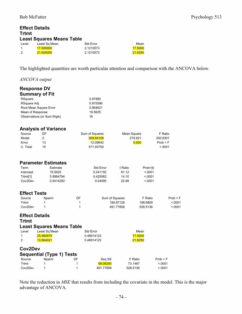
Bob McFatter Psychology 513
- 74 -
Effect DetailsTrtmtLeast Squares Means TableLevel Least Sq Mean Std Error Mean1 17.500000 2.1210573 17.50002 21.625000 2.1210573 21.6250
The highlighted quantities are worth particular attention and comparison with the ANCOVA below.
ANCOVA output
Response DVSummary of FitRSquare 0.97885RSquare Adj 0.975596Root Mean Square Error 0.964621Mean of Response 19.5625Observations (or Sum Wgts) 16
Analysis of VarianceSource DF Sum of Squares Mean Square F RatioModel 2 559.84108 279.921 300.8301Error 13 12.09642 0.930 Prob > FC. Total 15 571.93750 <.0001
Parameter EstimatesTerm Estimate Std Error t Ratio Prob>|t|Intercept 19.5625 0.241155 81.12 <.0001Trtmt[1] 5.9984794 0.425562 14.10 <.0001Cov2Dev 0.9414282 0.04095 22.99 <.0001
Effect TestsSource Nparm DF Sum of Squares F Ratio Prob > FTrtmt 1 1 184.87128 198.6809 <.0001Cov2Dev 1 1 491.77858 528.5136 <.0001
Effect DetailsTrtmtLeast Squares Means TableLevel Least Sq Mean Std Error Mean1 25.560979 0.48914123 17.50002 13.564021 0.48914123 21.6250
Cov2DevSequential (Type 1) TestsSource Nparm DF Seq SS F Ratio Prob > FTrtmt 1 1 68.06250 73.1467 <.0001Cov2Dev 1 1 491.77858 528.5136 <.0001
Note the reduction in MSE that results from including the covariate in the model. This is the major advantage of ANCOVA.
Bob McFatter Psychology 513
- 75 -
Lord’s Paradox
Bock (1975, Multivariate Statistical Methods in Behavioral Research, p. 490ff) describes what has come to be known as Lord’s Paradox:
Suppose a large university obtains measurements, at the beginning and end of the school year, of the weight of each student who takes his meals in the university dining halls. . . Suppose two statisticians analyze these data for differences in weight gain of men versus women. The first statistician analyzes simple gain scores [spring weight minus fall weight] and concludes that ‘as far as these data are concerned, there is no evidence of any interesting effect of the school diet (or of anything else) on student weight; in particular, there is no evidence of any differential effect on the two sexes, since neither group shows any systematic change.
The second statistician, on the other hand, decides to do an analysis of covariance. ‘After some necessary preliminaries, he determines that the slope of the regression line of final weight on initial weight is essentially the same for the two sexes. This is fortunate since it makes possible a fruitful comparison of the intercepts of the regression lines . . . He finds that the difference between the intercepts is statistically highly significant. The second statistician concludes . . . that the [men] showed significantly more gain in weight than the [women] when proper allowance is made for differences in initial weight between the two sexes.’ (from Lord, 1967)
As they are stated, the conclusions of the two statisticians are contradictory, and some form of paradox seems implied. On closer inspection, however, it is seen that these alternative methods of analyzing the data are actually directed toward different inferential problems. Moreover, each method provides the correct solution of the problem to which it is relevant.
These inferential problems may be described briefly as unconditional and conditional, respectively. The first statistician correctly analyzes gain scores to answer the unconditional question, “Is there a difference in the average gain in weight of the populations?” . . . The answer to this question, “No, there is no difference in average gain represented by the two sexes. At the same time, the second statistician correctly employs analysis of covariance to answer the conditional question, “Is a man expected to show a greater weight gain than a woman, given that they are initially of the same weight?” . . . The answer to this question is, “Yes, the man will be expected to gain more, for if he is initially of the same weight as the woman, he is either underweight and will be expected to gain, or the woman is overweight and will be expected to lose.” Because the regression lines are parallel, this expectation is independent of the given initial weight.

Bob McFatter Psychology 513
- 76 -
JMP example illustrating Lord’s paradox.
Sex Fall Spring D=Sp-FaMale 213 214 1Male 148 155 7Male 135 149 14Male 154 168 14Male 129 142 13Male 174 188 14Male 258 265 7Male 180 194 14Female 185 184 -1Female 108 112 4Female 101 112 11Female 153 164 11Female 95 93 -2Female 88 92 4Female 75 89 14Female 127 119 -8
Response D=Sp-FaSummary of Fit
RSquare 0.221042RSquare Adj 0.165402Root Mean Square Error 6.396846Mean of Response 7.3125Observations (or Sum Wgts) 16
Analysis of VarianceSource DF Sum of Squares Mean Square F RatioModel 1 162.56250 162.563 3.9727Error 14 572.87500 40.920 Prob > FC. Total 15 735.43750 0.0661
Parameter EstimatesTerm Estimate Std Error t Ratio Prob>|t|Intercept 7.3125 1.599212 4.57 0.0004Sex[Female] -3.1875 1.599212 -1.99 0.0661
Effect TestsSource Nparm DF Sum of Squares F Ratio Prob > FSex 1 1 162.56250 3.9727 0.0661Effect DetailsSexLeast Squares Means TableLevel Least Sq Mean Std Error MeanFemale 4.125000 2.2616267 4.1250Male 10.500000 2.2616267 10.5000

Bob McFatter Psychology 513
- 77 -
Response SpringRegression Plot
100
150
200
250
Spr
ing
50 100 150 200 250
Fall
Female
Male
Summary of Fit
RSquare 0.986965RSquare Adj 0.98496Root Mean Square Error 6.053748Mean of Response 152.5Observations (or Sum Wgts) 16
Analysis of VarianceSource DF Sum of Squares Mean Square F RatioModel 2 36073.578 18036.8 492.1648Error 13 476.422 36.6 Prob > FC. Total 15 36550.000 <.0001
Parameter EstimatesTerm Estimate Std Error t Ratio Prob>|t|Intercept 16.780885 6.029403 2.78 0.0155Fall 0.9347851 0.040199 23.25 <.0001Sex[Female] -5.058352 1.902727 -2.66 0.0197
Effect TestsSource Nparm DF Sum of Squares F Ratio Prob > FFall 1 1 19817.328 540.7499 <.0001Sex 1 1 259.008 7.0675 0.0197Effect DetailsFallSexLeast Squares Means TableLevel Least Sq Mean Std Error MeanFemale 147.44165 2.4312266 120.625Male 157.55835 2.4312266 184.375
Example with Both Interactions and Indicator Variables
Below is the SAS output for a regression analysis predicting positive emotional intensity (PI) from three predictors, extraversion (E), neuroticism (N), and sex (coded in various ways). E and N were standardized (M = 0, s = 1) prior to creating cross-products.
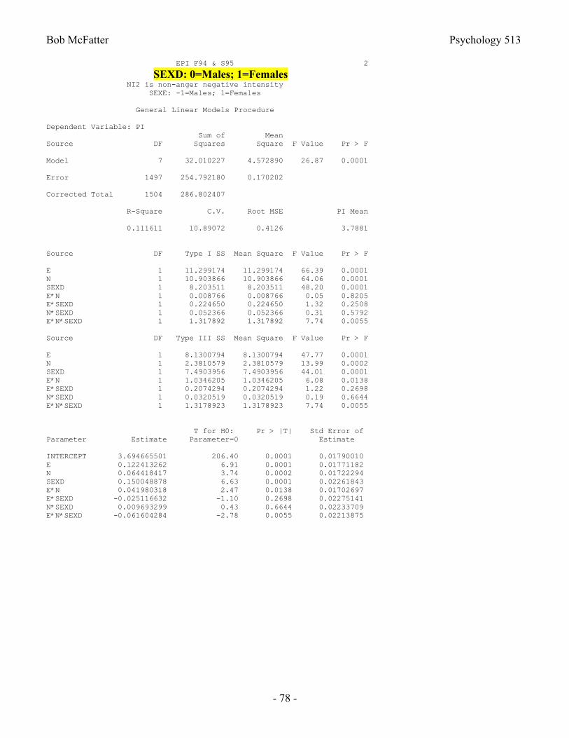
Bob McFatter Psychology 513
- 78 -
EPI F94 & S95 2
SEXD: 0=Males; 1=Females NI2 is non-anger negative intensity SEXE: -1=Males; 1=Females
General Linear Models Procedure
Dependent Variable: PI Sum of MeanSource DF Squares Square F Value Pr > F
Model 7 32.010227 4.572890 26.87 0.0001
Error 1497 254.792180 0.170202
Corrected Total 1504 286.802407
R-Square C.V. Root MSE PI Mean
0.111611 10.89072 0.4126 3.7881
Source DF Type I SS Mean Square F Value Pr > F
E 1 11.299174 11.299174 66.39 0.0001N 1 10.903866 10.903866 64.06 0.0001SEXD 1 8.203511 8.203511 48.20 0.0001E*N 1 0.008766 0.008766 0.05 0.8205E*SEXD 1 0.224650 0.224650 1.32 0.2508N*SEXD 1 0.052366 0.052366 0.31 0.5792E*N*SEXD 1 1.317892 1.317892 7.74 0.0055
Source DF Type III SS Mean Square F Value Pr > F
E 1 8.1300794 8.1300794 47.77 0.0001N 1 2.3810579 2.3810579 13.99 0.0002SEXD 1 7.4903956 7.4903956 44.01 0.0001E*N 1 1.0346205 1.0346205 6.08 0.0138E*SEXD 1 0.2074294 0.2074294 1.22 0.2698N*SEXD 1 0.0320519 0.0320519 0.19 0.6644E*N*SEXD 1 1.3178923 1.3178923 7.74 0.0055
T for H0: Pr > |T| Std Error ofParameter Estimate Parameter=0 Estimate
INTERCEPT 3.694665501 206.40 0.0001 0.01790010E 0.122413262 6.91 0.0001 0.01771182N 0.064418417 3.74 0.0002 0.01722294SEXD 0.150048878 6.63 0.0001 0.02261843E*N 0.041980318 2.47 0.0138 0.01702697E*SEXD -0.025116632 -1.10 0.2698 0.02275141N*SEXD 0.009693299 0.43 0.6644 0.02233709E*N*SEXD -0.061604284 -2.78 0.0055 0.02213875
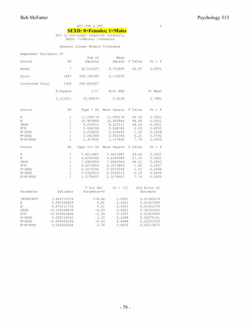
Bob McFatter Psychology 513
- 79 -
EPI F94 & S95 2
SEXD: 0=Females; 1=Males NI2 is non-anger negative intensity SEXE: -1=Males; 1=Females
General Linear Models Procedure
Dependent Variable: PI Sum of MeanSource DF Squares Square F Value Pr > F
Model 7 32.010227 4.572890 26.87 0.0001
Error 1497 254.792180 0.170202
Corrected Total 1504 286.802407
R-Square C.V. Root MSE PI Mean
0.111611 10.89072 0.4126 3.7881
Source DF Type I SS Mean Square F Value Pr > F
E 1 11.299174 11.299174 66.39 0.0001N 1 10.903866 10.903866 64.06 0.0001SEXD 1 8.203511 8.203511 48.20 0.0001E*N 1 0.008766 0.008766 0.05 0.8205E*SEXD 1 0.224650 0.224650 1.32 0.2508N*SEXD 1 0.052366 0.052366 0.31 0.5792E*N*SEXD 1 1.317892 1.317892 7.74 0.0055
Source DF Type III SS Mean Square F Value Pr > F
E 1 7.9013987 7.9013987 46.42 0.0001N 1 4.6206966 4.6206966 27.15 0.0001SEXD 1 7.4903956 7.4903956 44.01 0.0001E*N 1 0.3273855 0.3273855 1.92 0.1657E*SEXD 1 0.2074294 0.2074294 1.22 0.2698N*SEXD 1 0.0320519 0.0320519 0.19 0.6644E*N*SEXD 1 1.3178923 1.3178923 7.74 0.0055
T for H0: Pr > |T| Std Error ofParameter Estimate Parameter=0 Estimate
INTERCEPT 3.844714378 278.06 0.0001 0.01382679E 0.097296629 6.81 0.0001 0.01427999N 0.074111716 5.21 0.0001 0.01422379SEXD -0.150048878 -6.63 0.0001 0.02261843E*N -0.019623966 -1.39 0.1657 0.01414944E*SEXD 0.025116632 1.10 0.2698 0.02275141N*SEXD -0.009693299 -0.43 0.6644 0.02233709E*N*SEXD 0.061604284 2.78 0.0055 0.02213875

Bob McFatter Psychology 513
- 80 -
EPI F94 & S95 2 SEXD: 0=Males; 1=Females NI2 is non-anger negative intensity
SEXE: -1=Males; 1=Females
General Linear Models Procedure
Dependent Variable: PI Sum of MeanSource DF Squares Square F Value Pr > F
Model 7 32.010227 4.572890 26.87 0.0001
Error 1497 254.792180 0.170202
Corrected Total 1504 286.802407
R-Square C.V. Root MSE PI Mean
0.111611 10.89072 0.4126 3.7881
Source DF Type I SS Mean Square F Value Pr > F
E 1 11.299174 11.299174 66.39 0.0001N 1 10.903866 10.903866 64.06 0.0001SEXE 1 8.203511 8.203511 48.20 0.0001E*N 1 0.008766 0.008766 0.05 0.8205E*SEXE 1 0.224650 0.224650 1.32 0.2508N*SEXE 1 0.052366 0.052366 0.31 0.5792E*N*SEXE 1 1.317892 1.317892 7.74 0.0055
Source DF Type III SS Mean Square F Value Pr > F
E 1 15.872553 15.872553 93.26 0.0001N 1 6.546354 6.546354 38.46 0.0001SEXE 1 7.490396 7.490396 44.01 0.0001E*N 1 0.173564 0.173564 1.02 0.3127E*SEXE 1 0.207429 0.207429 1.22 0.2698N*SEXE 1 0.032052 0.032052 0.19 0.6644E*N*SEXE 1 1.317892 1.317892 7.74 0.0055
T for H0: Pr > |T| Std Error ofParameter Estimate Parameter=0 Estimate
INTERCEPT 3.769689940 333.33 0.0001 0.01130922E 0.109854945 9.66 0.0001 0.01137571N 0.069265066 6.20 0.0001 0.01116855SEXE 0.075024439 6.63 0.0001 0.01130922E*N 0.011178176 1.01 0.3127 0.01106938E*SEXE -0.012558316 -1.10 0.2698 0.01137571N*SEXE 0.004846650 0.43 0.6644 0.01116855E*N*SEXE -0.030802142 -2.78 0.0055 0.01106938
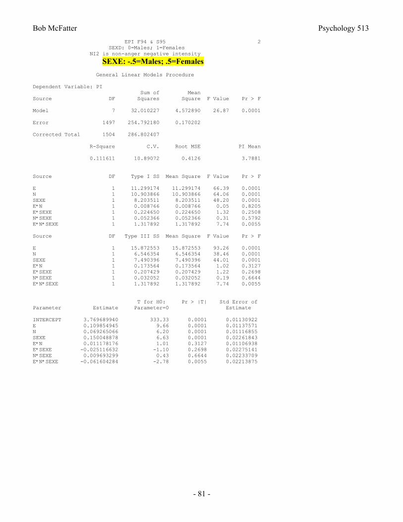
Bob McFatter Psychology 513
- 81 -
EPI F94 & S95 2 SEXD: 0=Males; 1=Females NI2 is non-anger negative intensity
SEXE: -.5=Males; .5=Females
General Linear Models Procedure
Dependent Variable: PI Sum of MeanSource DF Squares Square F Value Pr > F
Model 7 32.010227 4.572890 26.87 0.0001
Error 1497 254.792180 0.170202
Corrected Total 1504 286.802407
R-Square C.V. Root MSE PI Mean
0.111611 10.89072 0.4126 3.7881
Source DF Type I SS Mean Square F Value Pr > F
E 1 11.299174 11.299174 66.39 0.0001N 1 10.903866 10.903866 64.06 0.0001SEXE 1 8.203511 8.203511 48.20 0.0001E*N 1 0.008766 0.008766 0.05 0.8205E*SEXE 1 0.224650 0.224650 1.32 0.2508N*SEXE 1 0.052366 0.052366 0.31 0.5792E*N*SEXE 1 1.317892 1.317892 7.74 0.0055
Source DF Type III SS Mean Square F Value Pr > F
E 1 15.872553 15.872553 93.26 0.0001N 1 6.546354 6.546354 38.46 0.0001SEXE 1 7.490396 7.490396 44.01 0.0001E*N 1 0.173564 0.173564 1.02 0.3127E*SEXE 1 0.207429 0.207429 1.22 0.2698N*SEXE 1 0.032052 0.032052 0.19 0.6644E*N*SEXE 1 1.317892 1.317892 7.74 0.0055
T for H0: Pr > |T| Std Error ofParameter Estimate Parameter=0 Estimate
INTERCEPT 3.769689940 333.33 0.0001 0.01130922E 0.109854945 9.66 0.0001 0.01137571N 0.069265066 6.20 0.0001 0.01116855SEXE 0.150048878 6.63 0.0001 0.02261843E*N 0.011178176 1.01 0.3127 0.01106938E*SEXE -0.025116632 -1.10 0.2698 0.02275141N*SEXE 0.009693299 0.43 0.6644 0.02233709E*N*SEXE -0.061604284 -2.78 0.0055 0.02213875
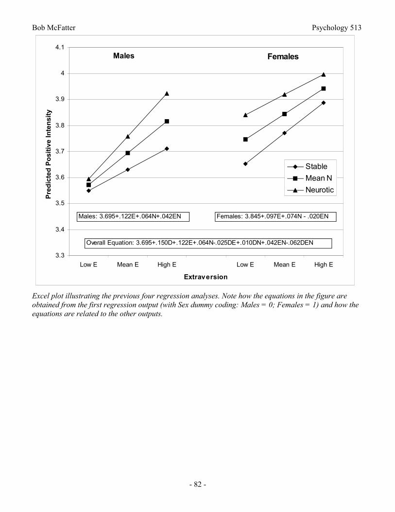
Bob McFatter Psychology 513
- 82 -
Excel plot illustrating the previous four regression analyses. Note how the equations in the figure are obtained from the first regression output (with Sex dummy coding: Males = 0; Females = 1) and how the equations are related to the other outputs.
3.3
3.4
3.5
3.6
3.7
3.8
3.9
4
4.1
Low E Mean E High E Low E Mean E High E
Extraversion
Pre
dic
ted
Po
siti
ve I
nte
nsi
ty
Stable
Mean N
Neurotic
Males Females
Overall Equation: 3.695+.150D+.122E+.064N-.025DE+.010DN+.042EN-.062DEN
Males: 3.695+.122E+.064N+.042EN Females: 3.845+.097E+.074N - .020EN
Bob McFatter Psychology 513
- 83 -
Interpretation of the Lower-Order Terms in the Output on p. 78
The intercept (3.695) in the regression equation reflects the predicted positive intensity (PI) score for males who are at the mean on both E and N because it is the predicted Y when all predictors are zero. The regression weight for E (0.1224) is the slope of the relation between E and PI for males (Sex = 0) who are at the mean on neuroticism (N = 0). An analogous interpretation applies to the weight for N. The weight for Sex (0.150) is the difference in predicted PI between males and females who are at the mean on both E and N, with the female predicted PI being 0.15 points higher than that for males. The interpretations of the 2-way interaction weights are given below in the discussion of the interpretation of the 3-way interaction.
Interpretation of the Two and Three-Way Interactions in the Output on p. 78
The 3-way interaction weight may be interpreted as the change in a 2-way interaction weight one would get for a one unit increase in the 3rd variable. That is, for example, the Sex E N weight reflects how the E N 2-way interaction weight changes for a one unit increase in Sex. Since Sex is dummy coded here (M = 0, F = 1), a one unit increase in Sex means the change in going from male to female. The 2-way E N weight for males in this output is 0.04198. This is the coefficient for males only because when Sex = 0 (males) the 3-way term goes away because it's multiplied by zero, and the only E N term left is 0.04198. When Sex = 1 (females) there are 2 E N terms in the equation: 0.04198 and -0.0616. The latter term becomes a simple E N term because it's multiplied by Sex, which is 1. Therefore, the 2-way E N term for females would thus be 0.04198 + (-0.0616) = -0.01962. These two E N weights in fact show up in the separate equations shown in the figure on p. 82. The difference between the two 2-way E N interaction weights is thus the 3-way interaction weight, and in this example it's highly significant. That means that the two E N interactions shown in the figure are significantly different from one another. The one for males is pretty pronounced with a positive fan shape (as reflected in the 0.04198). The one for females is less pronounced and has a negative fan shape (as reflected in the -0.01962).
Because the 3-way interaction is significant here, the interpretation of the E N interactions must be carried out separately for males and females. Interpreting the E N interaction for males (0.04198) would go something like this (it needs to be explicitly stated that all of the following applies only to males): The weight, 0.04198, reflects the increase in the slope of the relation between E and PI (positive intensity) that results from a one unit increase in N. Since E and N are standardized, one unit is one standard deviation. Thus, an increase of one standard deviation in N would lead to an increase of 0.04198 in the slope of the relation between E and PI. The slope of the relation between E and PI for males at the mean on N (N = 0) is 0.1224 (from the output). Thus, for males at the mean on N a one standard deviation increase in E would lead us to predict a 0.1224 point increase in positive intensity. However, for neurotic males at one standard deviation above the mean on N (N = 1), the slope of the relation between E and PI would be 0.1224 + 0.04198 = 0.16438. Thus, for neurotic males, a one standard deviation increase in E would lead us to predict a 0.16438 point increase in positive intensity. Thus, while the relation between extraversion and positive intensity is positive for both those at the mean on neuroticism and those at one standard deviation above the mean on neuroticism, that relation between E and PI is much stronger (and significantly so) for neurotics than for those at the mean on N.
Bob McFatter Psychology 513
- 84 -
Logistic Regression
If the criterion variable in a regression analysis is dichotomous (0, 1), then special considerations arise in the analysis. The predicted value of Y for any given X may be considered to be the probability that Ytakes on the value 1 for observations with the given X. As Kutner et al. point out, if one uses the ordinary simple linear regression model
Yi = β0 + β1 Xi + εi [61]
to analyze the data, at least three problems arise:
1) Nonnormal error terms2) Violation of the homoscedasticity assumption3) Predicted Ys that fall outside the 0 to 1 range.
The most common solution is to use a logistic response function rather than the simple linear model of equation [61] to model the data. The logistic response function (generalized to the case of several predictors) may be written as
exp
exp expY
b b X b X
b b X b X b b X b X
0 1 1 2 2
0 1 1 2 2 0 1 1 2 21
1
1
. [62]
This function is a monotonic, flattened S-shaped curve often called a sigmoidal curve which asymptotes at 0 and 1.
A nice property of the logistic response function is that it may be linearized by using the logit or log odds transform. If the predicted Y is considered to be the probability, p, of obtaining a 1 for the given value of X, and the model of equation [62] is assumed, then it can be shown that the natural log (i.e., logarithm to the base e) of the odds associated with p is a linear function of the Xs:
lnp
pb b X b X
1 0 1 1 2 2
[63]
The ratio p/(1 - p) is called the odds associated with the probability, p. Values for b0, b1, etc. may be obtained, usually by iterative maximum likelihood estimation, by many programs for logistic regression analysis. JMP will do logistic regression with one predictor in the Fit Y by X platform and many predictors in the Fit Model platform.
Odds and Probability
Because odds play such a prominent role in logistic regression and have properties that in some respects are nicer than those of probabilities, it is worth considering some of the characteristics of odds and their relation to probability. Odds are usually represented as a ratio of the chances of an event occurring to the chances of the event not occurring. For example, odds of 3:2 mean 3 chances out of 5 that the event occurs, 2 chances out of 5 the event doesn’t occur. One could represent this as a fraction, 3/2 = 1.5 or odds of 1.5:1, and the meaning would be the same. Notice that the probability of the event occurring would be 3/5 = .6, and the probability of the event not occurring would be 2/5 = .4.
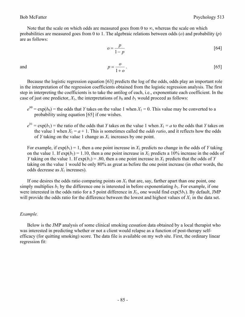
Bob McFatter Psychology 513
- 85 -
Note that the scale on which odds are measured goes from 0 to ∞, whereas the scale on which probabilities are measured goes from 0 to 1. The algebraic relations between odds (o) and probability (p) are as follows:
op
p
1[64]
and po
o
1. [65]
Because the logistic regression equation [63] predicts the log of the odds, odds play an important role in the interpretation of the regression coefficients obtained from the logistic regression analysis. The first step in interpreting the coefficients is to take the antilog of each, i.e., exponentiate each coefficient. In the case of just one predictor, X1, the interpretations of b0 and b1 would proceed as follows:
eb0 = exp(b0) = the odds that Y takes on the value 1 when X1 = 0. This value may be converted to a probability using equation [65] if one wishes.
eb1 = exp(b1) = the ratio of the odds that Y takes on the value 1 when X1 = a to the odds that Y takes on the value 1 when X1 = a + 1. This is sometimes called the odds ratio, and it reflects how the odds of Y taking on the value 1 change as X1 increases by one point.
For example, if exp(b1) = 1, then a one point increase in X1 predicts no change in the odds of Y taking on the value 1. If exp(b1) = 1.10, then a one point increase in X1 predicts a 10% increase in the odds of Y taking on the value 1. If exp(b1) = .80, then a one point increase in X1 predicts that the odds of Ytaking on the value 1 would be only 80% as great as before the one point increase (in other words, the odds decrease as X1 increases).
If one desires the odds ratio comparing points on X1 that are, say, farther apart than one point, one simply multiplies b1 by the difference one is interested in before exponentiating b1. For example, if one were interested in the odds ratio for a 5 point difference in X1, one would find exp(5b1). By default, JMP will provide the odds ratio for the difference between the lowest and highest values of X1 in the data set.
Example.
Below is the JMP analysis of some clinical smoking cessation data obtained by a local therapist who was interested in predicting whether or not a client would relapse as a function of post-therapy self-efficacy (for quitting smoking) score. The data file is available on my web site. First, the ordinary linear regression fit:
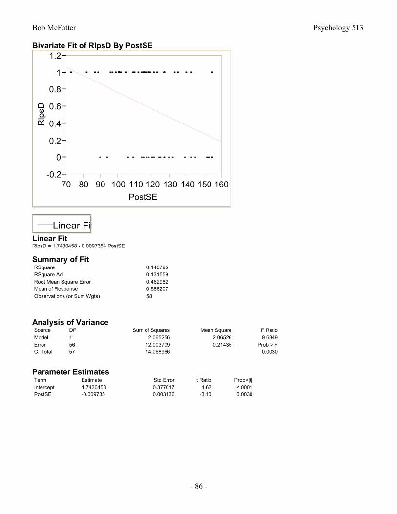
Bob McFatter Psychology 513
- 86 -
Bivariate Fit of RlpsD By PostSE
-0.2
0
0.2
0.4
0.6
0.8
1
1.2
Rlp
sD
70 80 90 100 110 120 130 140 150 160
PostSE
Linear FitLinear FitRlpsD = 1.7430458 - 0.0097354 PostSE
Summary of FitRSquare 0.146795RSquare Adj 0.131559Root Mean Square Error 0.462982Mean of Response 0.586207Observations (or Sum Wgts) 58
Analysis of VarianceSource DF Sum of Squares Mean Square F RatioModel 1 2.065256 2.06526 9.6349Error 56 12.003709 0.21435 Prob > FC. Total 57 14.068966 0.0030
Parameter EstimatesTerm Estimate Std Error t Ratio Prob>|t|Intercept 1.7430458 0.377617 4.62 <.0001PostSE -0.009735 0.003136 -3.10 0.0030
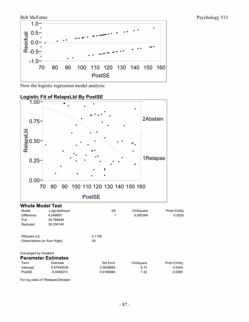
Bob McFatter Psychology 513
- 87 -
-1.0
-0.5
0.0
0.5
1.0R
esid
ual
70 80 90 100 110 120 130 140 150 160
PostSE
Now the logistic regression model analysis:
Logistic Fit of RelapsLbl By PostSE
Rel
apsL
bl
0.00
0.25
0.50
0.75
1.00
70 80 90 100 110 120 130 140 150 160
PostSE
1Relapse
2Abstain
Whole Model TestModel -LogLikelihood DF ChiSquare Prob>ChiSqDifference 4.546697 1 9.093394 0.0026Full 34.789448Reduced 39.336145
RSquare (U) 0.1156Observations (or Sum Wgts) 58
Converged by Gradient
Parameter EstimatesTerm Estimate Std Error ChiSquare Prob>ChiSqIntercept 5.87454534 2.0638865 8.10 0.0044PostSE -0.0460273 0.0168984 7.42 0.0065
For log odds of 1Relapse/2Abstain
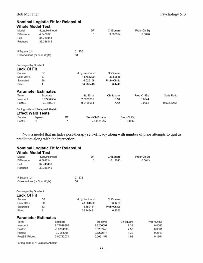
Bob McFatter Psychology 513
- 88 -
Nominal Logistic Fit for RelapsLblWhole Model TestModel -LogLikelihood DF ChiSquare Prob>ChiSqDifference 4.546697 1 9.093394 0.0026Full 34.789448Reduced 39.336145
RSquare (U) 0.1156Observations (or Sum Wgts) 58
Converged by Gradient
Lack Of FitSource DF -LogLikelihood ChiSquareLack Of Fit 37 18.764290 37.52858Saturated 38 16.025158 Prob>ChiSqFitted 1 34.789448 0.4449
Parameter EstimatesTerm Estimate Std Error ChiSquare Prob>ChiSq Odds RatioIntercept 5.87454534 2.0638865 8.10 0.0044 .PostSE -0.0460273 0.0168984 7.42 0.0065 0.02295465
For log odds of 1Relapse/2Abstain
Effect Wald TestsSource Nparm DF Wald ChiSquare Prob>ChiSqPostSE 1 1 7.41885645 0.0065
Now a model that includes post-therapy self-efficacy along with number of prior attempts to quit as predictors along with the interaction:
Nominal Logistic Fit for RelapsLblWhole Model TestModel -LogLikelihood DF ChiSquare Prob>ChiSqDifference 6.592714 3 13.18543 0.0043Full 32.743431Reduced 39.336145
RSquare (U) 0.1676Observations (or Sum Wgts) 58
Converged by Gradient
Lack Of FitSource DF -LogLikelihood ChiSquareLack Of Fit 50 28.061300 56.1226Saturated 53 4.682131 Prob>ChiSqFitted 3 32.743431 0.2562
Parameter EstimatesTerm Estimate Std Error ChiSquare Prob>ChiSqIntercept 8.77016896 3.2256597 7.39 0.0066PostSE -0.0734596 0.0267743 7.53 0.0061PriorAt -0.7084395 0.6222344 1.30 0.2549PostSE*PriorAt 0.00712071 0.0051451 1.92 0.1664
For log odds of 1Relapse/2Abstain

Bob McFatter Psychology 513
- 89 -
Effect Wald TestsSource Nparm DF Wald ChiSquare Prob>ChiSqPostSE 1 1 7.52766897 0.0061PriorAt 1 1 1.29627631 0.2549PostSE*PriorAt 1 1 1.91536066 0.1664
Excel may be used to get nice probability plots for logistic regression models as the following two Excel pages illustrate. Note the formula in the formula window for the selected cell in each worksheet.
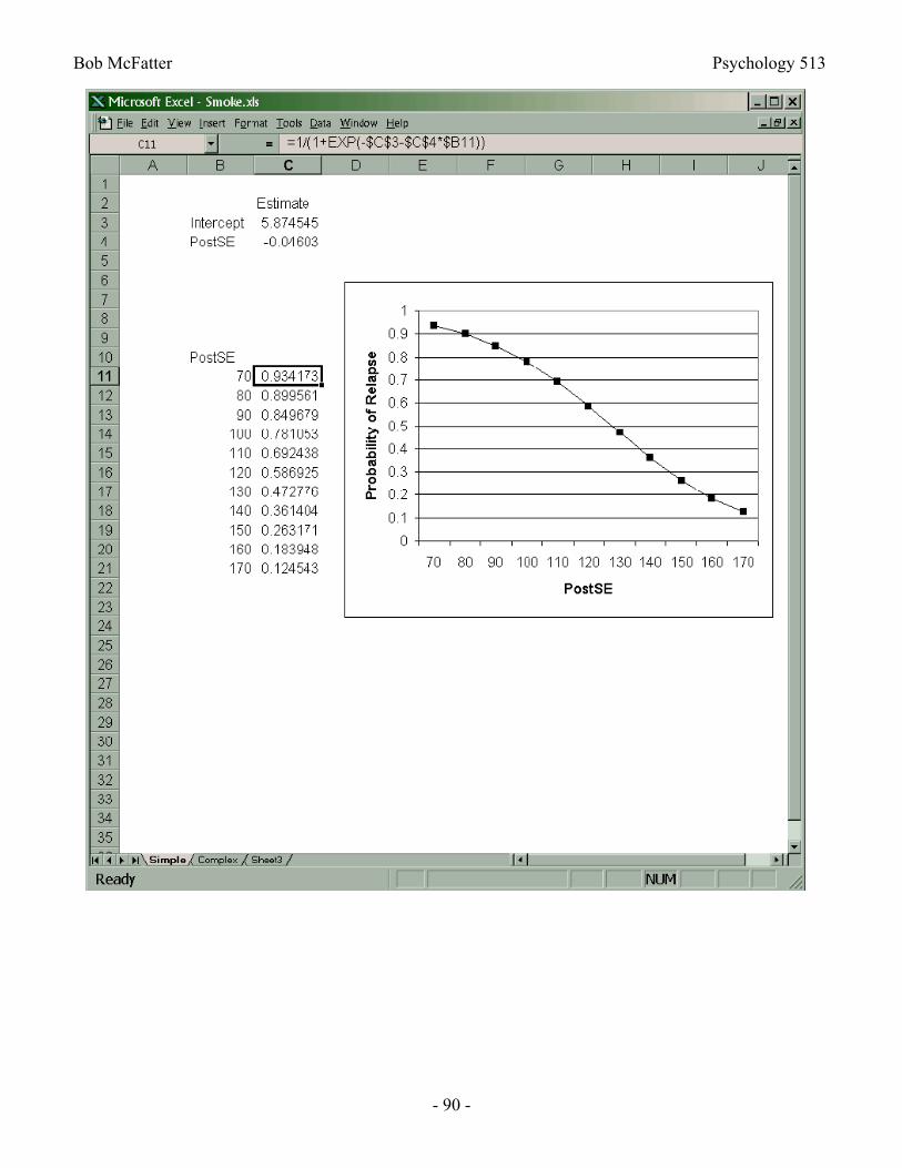
Bob McFatter Psychology 513
- 90 -
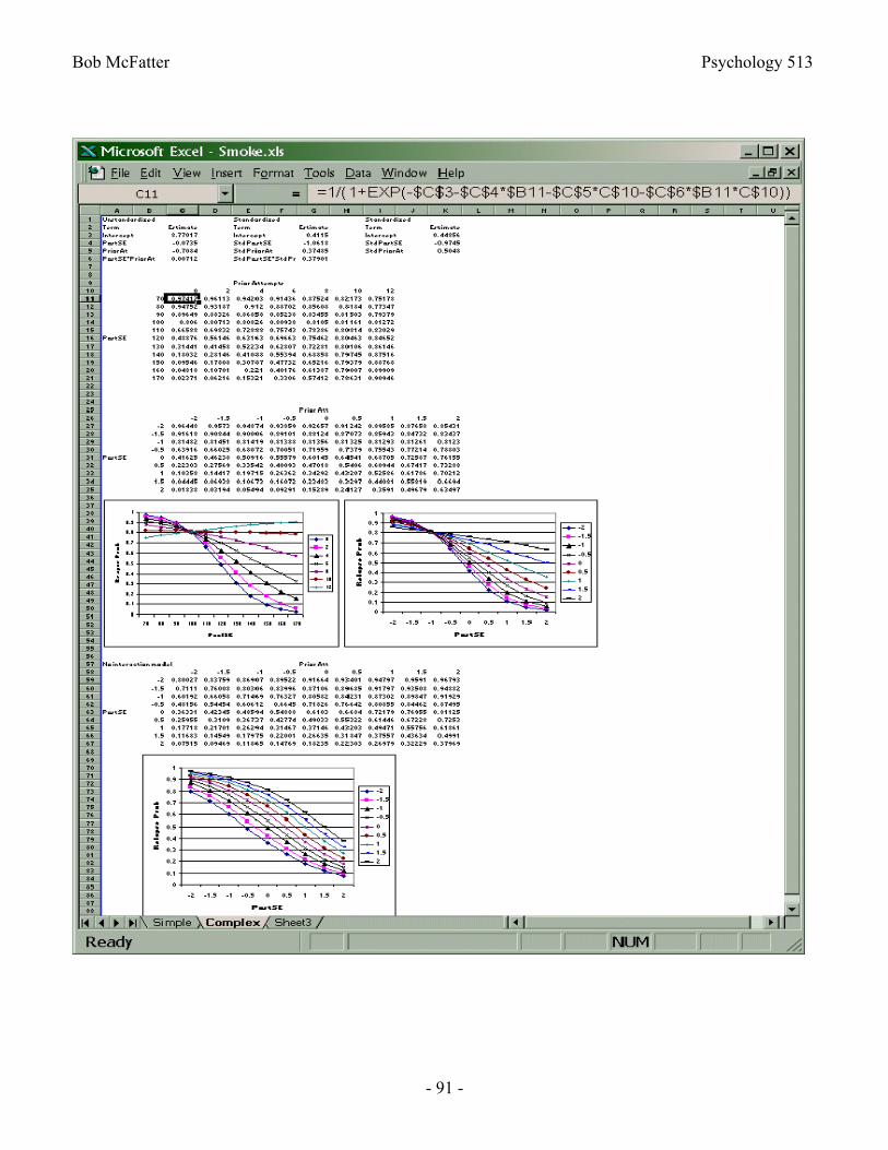
Bob McFatter Psychology 513
- 91 -