Embed Size (px)
Citation preview
1 PTAX I-E Intro to Sales Ratio Studies
January, 2017 PTAX-I-E (R-01/17)
I-E,
Introduction to
Sales Ratio
Studies

2 PTAX I-E Intro to Sales Ratio Studies
( Printed by the authority of the State of Illinois
( 35 copies – 02/14 - P.O. Number 2140251)
3 PTAX I-E Intro to Sales Ratio Studies
Course I-E Outline Introduction to Sales Ratio Studies
Glossary………………………………………………………………………………….. Page 4 Acronyms………………………………………………………………………………… Page 6 Where to get Assistance…………………………………………….......................... Page 7 UNIT 1 – Math Basics for Sales Ratio Studies…………………………………….. Page 8 Decimals and Percentages Averages Sales Ratio Quartile Ranges Interquartile Range UNIT 2 – The Sales Ratio Study……………………………………………………….Page 18 PTAX-203 Form/Assessment/Sales Ratio Study Verification of Sales Data Median Level of Assessment Trimming Urban Weighted Ratio UNIT 3 – Measures for the Uniformity of Assessments ………………………….Page 35 Coefficient of Dispersion Coefficient of Concentration Price Related Differential UNIT 4 – Equalization …………………………………………….…………………….Page 50 UNIT 5 – Assessor Bonus Award……………………………………………………..Page 61 UNIT 6 – Trending……………..…………………………………………………………Page 68 UNIT 7 – Sales Ratio Study: Table 1.…………………………………………………Page 83 Homework…………………………………………………………………………………Page 91 Individual Unit Review Questions and Exercise Answers..………………………Page 116 Sales Ratio Table 1 Information……………………………………..……………….. Page 154
4 PTAX I-E Intro to Sales Ratio Studies
CLASS GLOSSARY
Appraisal – an opinion of value, supported by evidence.
Assessed Value (AV) – the value placed on property for tax purposes and used as a basis for distribution of the tax burden. Most of the time this amount is subject to the State-issued equalization factor and the deduction of the homestead exemption on residential parcels. Assessment – the official act of discovering, listing, appraising and entering a value for property on the assessment rolls for ad valorem tax purposes. Assessment Level – refers to the statutory level of 33.33% or the actual level obtainable from a sales ratio study. Bank Real Estate Owned (REO) - the first sale of the property owned by a financial institution as a result of a judgment of foreclosure, transfer pursuant to a deed in lieu of foreclosure, or consent judgment, occurring after the foreclosure proceeding is complete. Coefficient of Concentration (COC) – the percentage of observations falling within 10% of the median level of assessments; a high COC indicates more uniformity. Coefficient of Dispersion (COD) - a statistical measure of variation of individual assessment ratios around the median level of assessments. An average error expressed as a percent of the median; an indicator of assessment uniformity found by dividing the average deviation by the median. It is the most common method used in measuring assessment uniformity. Equalized Assessed Value (EAV) – the assessed value multiplied by the State equalization factor. This gives the property value from which the tax rate is calculated after deducting all qualified homestead exemptions. For farm acreage, farm buildings, and coal rights, the final assessed value is the equalized assessed value. Individual tax bills are calculated by multiplying the individual district’s tax rates by the equalized assessed value after all qualifying exemptions have been removed. Equalization Multiplier – the application of a uniform percent increase or decrease to assessed values of various areas or classes of property to bring assessment levels to a uniform level of market value. The multiplier can be applied by Township Assessor (TA), Supervisor of Assessments (CCAO) or Board of Review (BR). Factor – represents the adjustment to an appraisal for any number of variables.
5 PTAX I-E Intro to Sales Ratio Studies
Market Value (Fair Cash Value) – the most probable sales price which a property should bring in a competitive and open market under all conditions requisite to a fair sale, the buyer and seller each acting prudently and knowledgeably, and assuming the price is not affected by undue stimulus. Mean – an arithmetic average. Median – the middle value of a ranked set of numbers. Mode – the number that occurs most frequently in a set of numbers. Outlier - a Sales Ratio (SR) whose results are a large deviation from the median; either below the median or above the median. Price-Related Differential (PRD) – any assessment bias related to the value of property. Quartiles – the values that divide a set of data into four equal parts (25%, 50%, 75%, 100%) when the data are arrayed in ascending order. Sale in Lieu of Foreclosure – a transfer pursuant to a deed in lieu of foreclosure if the Grantee is a financial institution. Sales Ratio (SR) – the ratio of assessed value to market value found from a property that has sold; ratio equals prior year (equalized) assessed value (AV or EAV) divided by the current year sales price (SP).
Sales Ratio Study – a analysis of the percentage relationship of assessed value to market value. Ratio equals prior year assessed value divided by the current year sales price. A minimum of 25 useable sales/appraisals is required. Short Sale – the property was sold for less than the amount owed to the mortgage lender or mortgagor, if the mortgagor has agreed to the sale. Urban Weighted Method – non-farm values; used in determining a county's median level of assessment by dividing the county's total assessed value (AV) by the county's total Estimate of Full Value (EFV); this is the preferred method of calculating a county multiplier.
6 PTAX I-E Intro to Sales Ratio Studies
ACRONYMS
AV = Assessed Value
Bank REO = Bank Real Estate Owned
BR = Board of Review
CCAO = Supervisor of Assessments, aka Chief County Assessing Officer
COC = Coefficient of Concentration
COD = Coefficient of Dispersion
DOR = Department of Revenue
EAV = Equalized Assessed Value
EFV = Estimate of Full Value
MV = Market Value (Fair Cash Value)
PRD = Price Related Differential
PTAB = Property Tax Appeal Board
RETD = Real Estate Transfer Declaration or PTAX 203 form
SP = Sales Price
SR = Sales Ratio
TA = Township Assessor
7 PTAX I-E Intro to Sales Ratio Studies
WHERE TO GET ASSISTANCE OR INFORMATION WEB LINKS
Property Tax Division: www.tax.illinois.gov/LocalGovernment/PropertyTax
Property Tax Code (35ILCS 200): www.ilga.gov
Illinois Property Tax Appeal Board: http://www.ptab.illinois.gov/
Real Estate Transfer Declaration Procedures for CCAO’s http://tax.illinois.gov/LocalGovernment/PropertyTax/CCAOProcedures.pdf
PUBLICATIONS
PTAX-1004 The Illinois Property Tax System http://tax.illinois.gov/Publications/LocalGovernment/PTAX1004.pdf
PTAX-136 Property Assessment and Equalization http://tax.illinois.gov/Publications/Pubs/Pub-136.pdf
8 PTAX I-E Intro to Sales Ratio Studies
Unit 1
Basic Math for Sales Ratio Studies This unit covers basic math calculations for Sales Ratio Studies.
Learning Objectives After completing this unit, you should be able to
Calculate a sales ratio
Explain the difference between mean, median and mode
Calculate averages
Explain the difference between decimals or percentages
Terms and Concepts
Decimals
Percentages
Average
Mean
Median
Mode
Sales Ratio
Quartiles
Interquartile Range
9 PTAX I-E Intro to Sales Ratio Studies
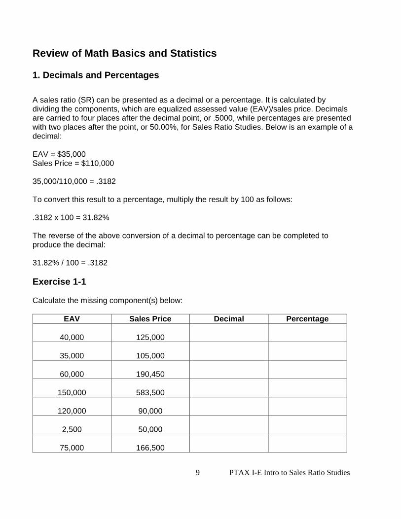
Review of Math Basics and Statistics 1. Decimals and Percentages
A sales ratio (SR) can be presented as a decimal or a percentage. It is calculated by dividing the components, which are equalized assessed value (EAV)/sales price. Decimals are carried to four places after the decimal point, or .5000, while percentages are presented with two places after the point, or 50.00%, for Sales Ratio Studies. Below is an example of a decimal:
EAV = $35,000 Sales Price = $110,000 35,000/110,000 = .3182 To convert this result to a percentage, multiply the result by 100 as follows: .3182 x 100 = 31.82% The reverse of the above conversion of a decimal to percentage can be completed to produce the decimal: 31.82% / 100 = .3182
Exercise 1-1 Calculate the missing component(s) below:
EAV Sales Price Decimal Percentage
40,000
125,000
35,000
105,000
60,000
190,450
150,000
583,500
120,000
90,000
2,500
50,000
75,000
166,500
10 PTAX I-E Intro to Sales Ratio Studies
2. Statistical Measures: Mean, Median and Mode The mean of a group of numbers, also called an array of numbers, represents the average of the entire group. To calculate the mean, add the entire array of numbers together and divide by the total number of the group. 2, 5, 10, 25, 50, 55, 70, 77, 110, 110, 150, 200 The average of this group of numbers is: 72 Add all of the numbers together for a total (864) and divide by the total numbers in the group (12). What does the result of 72 above represent for this group of numbers? The interpretation is that the average represents a centrally located result or if these numbers represented the SR calculated for a county, the average or mean for the county is an SR of 72%. The mean result for an array of numbers is sensitive to the range of the numbers. When the 150 and the 200 in the group of numbers is replaced with 7 and 139, what happens to the average for this group? Add the following numbers together and divide by 12 for the answer. 2, 5, 7, 10, 25, 50, 55, 70, 77, 110, 110, 139 The average of this group of numbers is: 55 The discussion then would be when comparing this mean to the statutory level of 33.33% that the county has considerable work to complete to bring the assessments to conform to the required level. But, does that make sense in terms of the mean being a reasonably accurate result for a central point of tendency? Another statistical measure that would provide a more practical result when discussing Sales Ratio Studies is the median. This is the middle occurrence for the total group of SR for a county. Using the first set of numbers as the guide, what is the median?
Exercise 1-2 Median = ______________ Note: To find the median in an odd numbered group, find the middle result after the numbers are sorted in ascending order. For groups of numbers with an even amount in the array, locate the two middle results, add together and divide the answer by two.
11 PTAX I-E Intro to Sales Ratio Studies
Exercise 1-3 The final statistical centrally located result when evaluating SR is the mode. This is the number that is displayed the most in an array of figures. Using the first or second set of numbers above, what would the mode be? ______________
3. Sales Ratio (SR) The calculation of an SR uses the following formula: EAV / Sales Price (SP) = SR You will notice this was used when discussing the basic math of decimal and percentage calculations previously. The information can be found within the County’s assessment records and on the RETD that’s recorded for the sale of property.
Exercise 1-4 Specifically, the EAV represents the final, Board of Review certified assessment from the prior year. If the sale for a property is being recorded in 2015, what assessment year should be used? Deed for the sale is dated: 2015 = _______ Assessment Deed for the sale is dated: 2012 = _______ Assessment Deed for the sale is dated: 2014 = _______ Assessment Deed for the sale is dated: 2016 = _______ Assessment
12 PTAX I-E Intro to Sales Ratio Studies
4. Quartiles Quartiles divide the array of data into four equal quarters. The first quartile is where the lowest 25% of the observations would fall. The second quartile is where the median would be located and the third quartile is where 75% of the observations would fall below. Examples for calculating quartiles: The first quartile for an array of numbers with a set of data of 75 is: (0.25)(75) + 0.25 = 19 This result indicates that 25% of this particular set of data falls below the score of 19. The third quartile for an array of numbers with a set of date of 75 is: (0.75)(75) + 0.75 = 57 This result indicates that 75% of results for this particular set of data falls below the score of 57.
Exercise 1-5 Answer the questions for following array of numbers. 19.25, 22.46, 32.57, 32.99, 34.20, 36.59, 36.59, 37.46, 37.89, 38.80, 38.99, 39.99, 42.76, 44.98, 87.25 What is the First Quartile in the above group of numbers? (0.__)(15) + 0.__ = ___ What is the Third Quartile in the above group of numbers? (0.__)(15) + 0.__ = ___ The consequence of the quartile results produced in a sales ratio study is to apply the outcome to identify outliers and remove them from the study. These outliers are felt to distort the study’s results and can be caused by a number of attributes:
The assessed value from the prior year is not in sync with the current year’s sales price. The sales price could be higher because of major remodeling, for example. The
13 PTAX I-E Intro to Sales Ratio Studies
sales price could also be lower based on the house remaining vacant for a number of years.
The inadvertent use of a sale that does not represent an arm’s length transaction. The sale may have occurred between a father and his married daughter (with a different last name) and if the preparer did not indicate they were relatives, this sale may end up on the sales ratio study.
An error in the assessed value provided by the CCAO’s office on the PTAX 203 form. The office may have accidentally not provided the prior year’s Board of Review EAV.
5. Interquartile Range The interquartile range is used when calculating the sales ratios that are identified as outliers for the sales ratio study. The difference between the first and third quartiles represents the interquartile range. From the above calculations for the first and third quartile, we found that the first quartile result was 32.99 and the third quartile result was 39.99. The interquartile range in this example is 7.00. When evaluating the sales ratio results for your township, the interquartile range is multiplied by 6 with a result of 42.00 in this instance. The 42.00 is added to the 39.99 to find the upper trim point or 81.99. This same process is applied to calculate the lower trim point or 42.00 is subtracted from 32.99 for the lower trim point of -9.01. Following through then, any sales ratio above 81.99 is removed from the study and any sales ratio below -9.01 (there would not be a negative sales ratio so there wouldn’t be a removal for this result) are removed from the study as well. Third Quartile – First Quartile = Interquartile Range Interquartile Range x 6 = Result Third Quartile + Result = Upper Trim Limit First Quartile – Result = Lower Trim Limit
Exercise 1-6 From the above example, were there any sales removed from this study? __________ For the above example, what is the ratio range for this township before removal of outliers? _____ after the removal of outliers? ___________ What was the median for this set of data before removal of any outliers? _________ What is the median for set of data after removal of outliers, if applicable? _________
14 PTAX I-E Intro to Sales Ratio Studies
Exercise 1-7 Answer the questions for the following array of numbers. 15.25, 25.46, 26.57, 38.99, 39.20, 39.59, 39.59, 41.46, 43.89, 44.80, 45.99, 45.99, 50.76, 90.98, 107.25 From the above example, were there any sales removed from this study? __________ For the above example, what is the ratio range for this township before removal of outliers? _____ after the removal of outliers? ___________ What was the median for this set of data before removal of any outliers? _________ What is the median for set of data after removal of outliers, if applicable? _________
Exercise 1-8
2.38, 21.46, 26.57, 38.99, 39.20, 39.59, 39.59, 41.46, 43.89, 45.80, 45.99, 45.99, 50.76, 54.85, 55.67, 79.88, 90.98, 157.25, 166.88 From the above example, were there any sales removed from this study? __________ For the above example, what is the ratio range for this township before removal of outliers? _____ after the removal of outliers? ___________ What was the median for this set of data before removal of any outliers? _________ What is the median for set of data after removal of outliers, if applicable? _________
Exercise 1-9
1.25, 25.46, 26.57, 38.99, 39.20, 39.59, 39.59, 41.46, 43.89, 44.80, 45.99, 45.99, 50.76, 88.92, 127.25 From the above example, were there any sales removed from this study? __________ For the above example, what is the ratio range for this township before removal of outliers? _____ after the removal of outliers? ___________ What was the median for this set of data before removal of any outliers? _________ What is the median for set of data after removal of outliers, if applicable? _________
15 PTAX I-E Intro to Sales Ratio Studies
Exercise 1-10
15.25, 25.46, 26.57, 38.99, 39.20, 39.59, 39.59, 40.72, 41.46, 43.89, 44.80, 45.99, 45.99, 50.76, 75.98, 107.25, 110.68, 111.25, 138.55 From the above example, were there any sales removed from this study? __________ For the above example, what is the ratio range for this township before removal of outliers? _____ after the removal of outliers? ___________ What was the median for this set of data before removal of any outliers? _________ What is the median for set of data after removal of outliers, if applicable? _________
Exercise 1-11
1.25, 4.38, 5.50, 15.25, 25.46, 36.57, 38.99, 39.20, 39.59, 39.59, 40.99, 41.46, 42.66, 43.89, 44.80, 45.99, 45.99, 49.98, 50.76, 75.22, 90.98, 97.25, 145.33 From the above example, were there any sales removed from this study? __________ For the above example, what is the ratio range for this township before removal of outliers? _____ after the removal of outliers? ___________ What was the median for this set of data before removal of any outliers? _________ What is the median for set of data after removal of outliers, if applicable? _________
16 PTAX I-E Intro to Sales Ratio Studies
Summary
The basic math for sales ratio studies include calculated results being expressed as either decimals, .4526, or percentages, 45.26%. When a decimal is presented as a percentage, multiply the result by 100. The reverse is true for presenting a percentage as a decimal, or dividing the result by 100. Measures for the point of central tendency include the mean (average), the median and the mode for an array of numbers. The mean is calculated by adding all of the results together and dividing by the total number in the array. The median represents the central point within an array of numbers. To find the median, arrange the results in ascending order and for an odd number, find the middle point. For an even number of results within an array and after arranging in ascending order, locate the two middle results, add together and divide by 2. The final point of central tendency is the mode. The mode represents the number within an array that is presented the most number of times. Quartile ranges divide an array of numbers into four equal parts. The importance or the part these quartile ranges play in a sales ratio study is that they are used in the calculation that will ‘trim’ sales ratios that are outside the calculated range. Interquartile range is the distance between the first and third quartiles. Used in the calculation for the lower and upper limits of outliers. An additional component of the calculation to identify outliers on a sales ratio study is the interquartile range. This represents the difference between the first and third quartiles after the sales ratios are arranged in ascending order. To calculate the lower and upper trim points is completed with the following formula: Third Quartile – First Quartile = Interquartile Range Interquartile Range x 6 = Result Third Quartile + Result = Upper Trim Limit First Quartile – Result = Lower Trim Limit
17 PTAX I-E Intro to Sales Ratio Studies
UNIT 1 Review Questions
1. T or F To calculate a sales ratio, the EAV is divided by the sales price.
2. T or F The mode for an array of numbers is the result located in the middle.
3. T or F A median is the number that shows up in an array of numbers the most
times.
4. T or F Quartile ranges play no significant role in the sales ratio process.
5. T or F The formula to calculate a sales ratio contains the current year’s EAV
divided by the prior year’s sales price.
6. What central point of tendency reflects the middle sales ratio result?
____________
7. Calculate the lower and upper trim points from the following array of 15 numbers.
2.00, 15.46, 24.80, 24.80, 25.08, 26.10, 32.99, 33.24, 33.24, 34.15, 36.77, 50.86,
51.33, 77. 33, 105.66
From your results, what, if any ratios will be removed from the data? _________
18 PTAX I-E Intro to Sales Ratio Studies
Unit 2
PTAX-203 Form/The Sales Ratio Study This unit discusses the PTAX-203 form, focusing on the information gathered on these documents and determines through editing procedures whether a sale is to be included in or excluded from the sales ratio study. This chapter will also provide a discussion for sales transactions that represent arm’s length characteristics and those transactions that do not. The importance of removing sales that are not arm’s length or valid sales is also discussed. Once the valid sales are identified through the Department’s editing processes the discussion moves towards the uses for Sales Ratio Studies, including a basic understanding of the process for determining a median level of assessment, assessment uniformity, the appeal process for issues relating to the assessment value of property and as a basis for the determination of the assessor bonus award and the partial reimbursement of the supervisor of assessment’s salary.
Learning Objectives After completing this unit, you should be able to
Become familiar with PTAX-203 form
Understand the requirements for an arm’s length transaction
Identify several uses for the sales ratio study
Identify criteria for the development of the sales ratio study
Determine the median level of assessments
Verify the PTAX-203 information
Calculate sales ratios
Determine the outlier ratios to remove from sales ratio study
Terms and Concepts
Arm’s length transaction
Median
Median level
Rank
Sales Ratio
Trimming
19 PTAX I-E Intro to Sales Ratio Studies
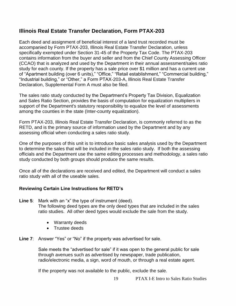
Illinois Real Estate Transfer Declaration, Form PTAX-203 Each deed and assignment of beneficial interest of a land trust recorded must be accompanied by Form PTAX-203, Illinois Real Estate Transfer Declaration, unless specifically exempted under Section 31-45 of the Property Tax Code. The PTAX-203 contains information from the buyer and seller and from the Chief County Assessing Officer (CCAO) that is analyzed and used by the Department in their annual assessment/sales ratio study for each county. If the property has a sale price over $1 million and has a current use of “Apartment building (over 6 units),” “Office,” “Retail establishment,” “Commercial building,” “Industrial building,” or “Other,” a Form PTAX-203-A, Illinois Real Estate Transfer Declaration, Supplemental Form A must also be filed. The sales ratio study conducted by the Department’s Property Tax Division, Equalization and Sales Ratio Section, provides the basis of computation for equalization multipliers in support of the Department's statutory responsibility to equalize the level of assessments among the counties in the state (Inter-county equalization). Form PTAX-203, Illinois Real Estate Transfer Declaration, is commonly referred to as the RETD, and is the primary source of information used by the Department and by any assessing official when conducting a sales ratio study. One of the purposes of this unit is to introduce basic sales analysis used by the Department to determine the sales that will be included in the sales ratio study. If both the assessing officials and the Department use the same editing processes and methodology, a sales ratio study conducted by both groups should produce the same results.
Once all of the declarations are received and edited, the Department will conduct a sales ratio study with all of the useable sales.
Reviewing Certain Line Instructions for RETD’s
Line 5: Mark with an “x” the type of instrument (deed). The following deed types are the only deed types that are included in the sales ratio studies. All other deed types would exclude the sale from the study.
Warranty deeds
Trustee deeds Line 7: Answer “Yes” or “No” if the property was advertised for sale.
Sale meets the “advertised for sale” if it was open to the general public for sale through avenues such as advertised by newspaper, trade publication, radio/electronic media, a sign, word of mouth, or through a real estate agent. If the property was not available to the public, exclude the sale.
20 PTAX I-E Intro to Sales Ratio Studies
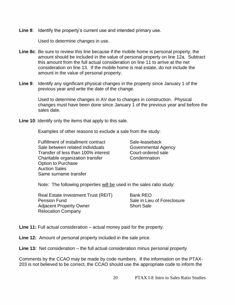
Line 8: Identify the property’s current use and intended primary use. Used to determine changes in use.
Line 8c: Be sure to review this line because if the mobile home is personal property, the
amount should be included in the value of personal property on line 12a. Subtract this amount from the full actual consideration on line 11 to arrive at the net consideration on line 13. If the mobile home is real estate, do not include the amount in the value of personal property.
Line 9: Identify any significant physical changes in the property since January 1 of the
previous year and write the date of the change. Used to determine changes in AV due to changes in construction. Physical changes must have been done since January 1 of the previous year and before the sales date.
Line 10: Identify only the items that apply to this sale.
Examples of other reasons to exclude a sale from the study: Fulfillment of installment contract Sale-leaseback Sale between related individuals Governmental Agency Transfer of less than 100% interest Court-ordered sale Charitable organization transfer Condemnation Option to Purchase Auction Sales Same surname transfer Note: The following properties will be used in the sales ratio study: Real Estate Investment Trust (REIT) Bank REO Pension Fund Sale in Lieu of Foreclosure Adjacent Property Owner Short Sale Relocation Company
Line 11: Full actual consideration – actual money paid for the property.
Line 12: Amount of personal property included in the sale price.
Line 13: Net consideration – the full actual consideration minus personal property
Comments by the CCAO may be made by code numbers. If the information on the PTAX-203 is not believed to be correct, the CCAO should use the appropriate code to inform the
21 PTAX I-E Intro to Sales Ratio Studies
Department. These codes are located in the “Real Estate Transfer Declaration Procedures for CCAOs” manual that can be found on the Department’s website.
The Assessment/Sales Ratio Study The primary tool the equalization process utilizes is the sales ratio study. The Sales Ratio Study provides the Median Level of Assessments for a specific jurisdiction for the year of the study. This study provides information on the percentage relationship of assessed value to market value for real property in certain categories and geographic areas. Information is also provided on the variation in assessment levels among and within these categories and geographic areas. The year of the sales ratio study refers to the year in which the sales occurred. So, the 2015 sales ratio study refers to sales from 2015 and the assessed values applied to those same sales from the prior year, 2014. The attributes that allow a sale of property to be included or excluded from the Sales Ratio Study is based on the idea of what the market value or full value of a property is. Market value –the most probable price which a property should bring in a competitive and open market under all conditions requisite to a fair sale, the buyer and seller each acting prudently and knowledgeably, and assuming the price is not affected by undue stimulus. Some types of sales included in the sales ratio study would be:
1. Arm’s Length Transactions.
buyer and seller are motivated;
both parties are well informed or well advised and acting in what they consider their best interests;
a reasonable time is allowed for exposure in the open market; o While a reasonable length of time can be a subjective attribute because
there is no definitive hard and fast rule guiding what is reasonable, the following lists the types of advertising considered acceptable with no discussion on the length of time:
Advertised via an MLS listing or with a Realtor Advertised by word of mouth Advertised by owner placing ‘For Sale’ sign in front yard Advertising via the internet
payment is made in terms of cash in United States dollars or in terms of financial arrangements comparable thereto; and
the price represents the normal consideration for the property sold unaffected by anyone associated with the sale.
The transaction is one between unrelated parties or parties not under abnormal pressure from each other.
2. Current year sales with prior year assessment values.
3. Sales that used either Warranty or Trustee deeds to record the transaction.
22 PTAX I-E Intro to Sales Ratio Studies
Some types of sales excluded from the sales ratio study would be:
1. Sales that are not Arm’s Length Transactions.
Not advertised for sale
Family transfer (same surname)
Transfer to a bank, credit union, or savings and loan
Transfer in Lieu of Foreclosure (different than a sale in lieu of foreclosure which is left in the sales ratio study per statute)
Sheriff’s deed
Court Officer’s deed
Transfers to a Governmental unit
2. A prior year sale recorded in the current year.
3. Sales where the prior year’s assessed value and the sales price are not comparable.
A new improvement was added
Property was demolished
Partial or pro-rated assessment
Sale involved exempt or specially-assessed property Core facts for the above definition of market value are:
The buyer and seller are knowledgeable about the property.
The buyer and seller are acting in their best interests.
The property has been advertised on the market for a reasonable length of time.
The consideration can be in the form of cash or other agreed upon value.
In addition to the idea of receiving and paying, the market value for a property is the discussion of the type of deed that’s used in the conveyance of title for the property. The Warranty (including the Corporation Warranty) and Trustee deeds are the only two types of deed that will grant all rights to the ownership of the property, free and clear of encumbrances or breaks in the line of title and included in the sales ratio study. The following is a list of deeds that are excluded from the sales ratio study: Limited Warranty Deed Special Warranty Deed Deed in Trust Quit Claim Deed Court Officer's Deed Master's Deed Special Commissioner Deed Administrator's Deed Guardian's Deed Conservator's Deed Sheriff’s Deed Cemetery Lots (Exempt)
23 PTAX I-E Intro to Sales Ratio Studies
The following is a list of additional attributes that will remove a sale from the sales ratio study: Family (same surname) Transfer Re-Recording of Document Sheriff's Deed Timber Rights-Mineral Rights Transfers to Government Unit Transfer to a Hospital Transfers to/from Charitable Organizations Auction Sales Supplemental Deed Given to Correct an Error in Previous Deed Conveyance of Less than Full Interest Transfers Assignments of Beneficial Interest of a Land Trust Sale that includes exchange of real estate
The sales ratio study results can provide information for:
1. In the review and appeal of assessments. The sales ratio studies provide a measure of the average assessment level for a given geographic area or category of property against which assessments of individual parcels may be judged in determining the degree of over or understatement, if any. One of the reasons to appeal an assessment is that the level of assessment on the property is higher than the township or county median level of assessments.
2. As a diagnostic tool to evaluate local assessment practices. It is the responsibility of local assessing officials to use the assessment/sales ratio study to evaluate their assessment policies and make assessment changes to sales and non-sales when warranted so that the final assessment of all properties in their jurisdictions are at a uniform percentage of value. Certain measures of assessment uniformity (coefficient of dispersion, coefficient of concentration, median absolute deviation) are based on the median level of assessments. A sales ratio study can be completed at any time and even multiple times throughout the year to support the evaluation of the trending for the real estate market. Studies that gather information on current sales for a particular neighborhood, subdivision, location/proximity that make the properties more desirable and other characteristics of properties within the township are just a few viable possibilities.
3. To determine eligibility for the assessor bonus award. In order to qualify for the assessor bonus award, the average of the median levels of assessments of the prior 3 years must be between 31.33% and 35.33% and the Coefficient of Dispersion (COD) must be below the appropriate COD as determined by the population of the county.
4. In reimbursement to a county of a portion of the Supervisor of Assessment’s salary. In order to qualify for the reimbursement to the county, the average of the median levels of assessments of the prior 3 years must be between 31.33% and 35.33%.
24 PTAX I-E Intro to Sales Ratio Studies
Verification of Property Sale Data The process of verifying the accuracy of information that preparers place on the PTAX-203 form is important and has various implications when the information is left incorrect. All information can be verified as soon as possible after a sale occurs and be communicated back to the CCAO’s office. Items to review would include but should not be limited to the following actions.
Verify that the parcel identification number (PIN) is correct for the property being sold.
Confirm the address, date of deed (date which deed was signed by parties to the transaction) and type of property.
Verify that any specific attributes to the sale are indicated in Step 1, Lines 9 and 10 (Line 9 – major remodeling would be the removal of walls and addition of rooms, for example. This would not include painting, new floors, new kitchen/bathroom fixtures which are considered maintenance. The best proof for major remodeling would be a building permit or letter from the seller/buyer stating the work specifically completed for review by the Department).
Review whether there would be a reason that the sales price does not coincide with the assessed value.
Review the legal description to verify it is referencing the property being sold.
Verify the seller and buyer information as well as the preparer information. The timing of the corrections needs to occur before the Department prepares the sales ratio study for the year of the sale. For example, a sale that occurred in 2015 should be corrected before the 2015 sales ratio study is completed. The CCAO is provided with the detail listing for the county, broken down by township for review. The CCAO can provide the sales that the Department is proposing to use for review to the Township Assessor and if there is a valid reason for removing a sale (or adding a sale), proof will have to accompany the request for removal from the CCAO’s office back to the Department. The Department will then review the information provided and based on procedures, make the decision to either remove the sale or add the sale. By providing corrections in a timely manner to the CCAO’s office, this will ensure that the Department is using the same set of sales for all programs that utilize those results.
Median Level of Assessments Chapter 1 of this course provided the formula for calculating the sales ratio as follows: EAV / Sales Price = Sales Ratio This is a straightforward formula, but remember that the final Board of Review certified prior year EAV is to be used.
25 PTAX I-E Intro to Sales Ratio Studies
The median of the sales ratios will be determined using the sales from the current year and the assessed values from the prior year for those transactions that have been determined to be market value. The median is the middle number in a set of numbers that have been ranked (placed in order). If there are an even number of ratios, the median will be the average of the two middle numbers. For example, if a property assessed at $38,600 in one year and sold for $120,000 in the following year, the sales ratio would be 32.17 %. Sales Ratio = 38,600 X 100 (%) = 32.17 % 120,000 Steps to calculate a median:
Calculate a sales ratio for each sale using the formula above.
Rank the sales ratios.
Determine the median. (Find the middle ratio.)
26 PTAX I-E Intro to Sales Ratio Studies
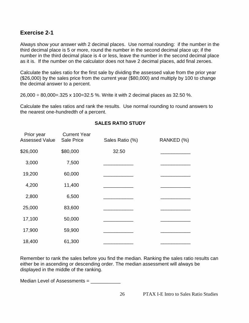
Exercise 2-1 Always show your answer with 2 decimal places. Use normal rounding: if the number in the third decimal place is 5 or more, round the number in the second decimal place up; if the number in the third decimal place is 4 or less, leave the number in the second decimal place as it is. If the number on the calculator does not have 2 decimal places, add final zeroes. Calculate the sales ratio for the first sale by dividing the assessed value from the prior year ($26,000) by the sales price from the current year ($80,000) and multiply by 100 to change the decimal answer to a percent. 26,000 ÷ 80,000=.325 x 100=32.5 %. Write it with 2 decimal places as 32.50 %. Calculate the sales ratios and rank the results. Use normal rounding to round answers to the nearest one-hundredth of a percent. SALES RATIO STUDY Prior year Current Year Assessed Value Sale Price Sales Ratio (%) RANKED (%) $26,000 $80,000 32.50 ___________ 3,000 7,500 ___________ ___________ 19,200 60,000 ___________ ___________ 4,200 11,400 ___________ ___________ 2,800 6,500 ___________ ___________ 25,000 83,600 ___________ ___________ 17,100 50,000 ___________ ___________ 17,900 59,900 ___________ ___________ 18,400 61,300 ___________ ___________ Remember to rank the sales before you find the median. Ranking the sales ratio results can either be in ascending or descending order. The median assessment will always be displayed in the middle of the ranking. Median Level of Assessments = ___________
27 PTAX I-E Intro to Sales Ratio Studies
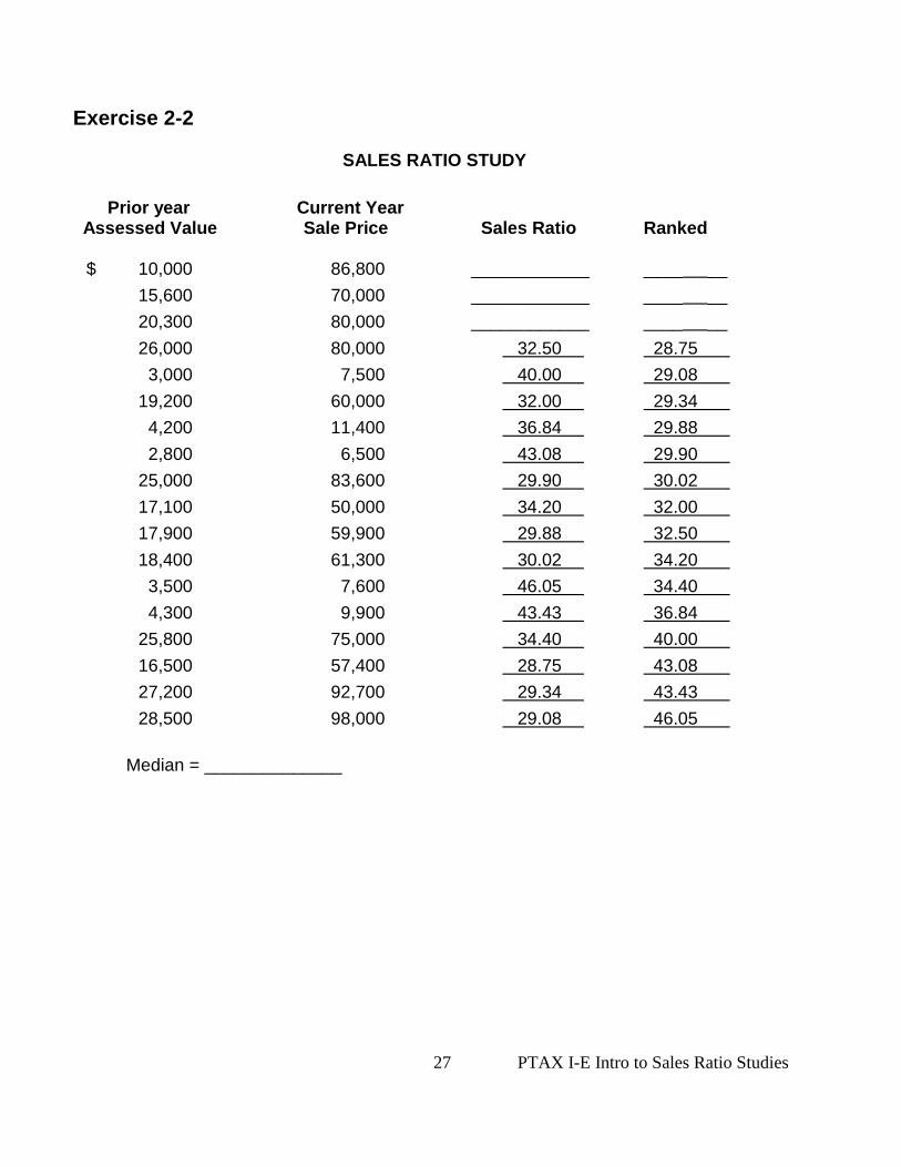
Exercise 2-2
SALES RATIO STUDY
Prior year Current Year
Assessed Value Sale Price Sales Ratio Ranked $ 10,000 86,800 ____________ ____ __
15,600 70,000 ____________ ____ __
20,300 80,000 ____________ ____ __
26,000 80,000 32.50 28.75
3,000 7,500 40.00 29.08
19,200 60,000 32.00 29.34
4,200 11,400 36.84 29.88
2,800 6,500 43.08 29.90
25,000 83,600 29.90 30.02
17,100 50,000 34.20 32.00
17,900 59,900 29.88 32.50
18,400 61,300 30.02 34.20
3,500 7,600 46.05 34.40
4,300 9,900 43.43 36.84
25,800 75,000 34.40 40.00
16,500 57,400 28.75 43.08
27,200 92,700 29.34 43.43
28,500 98,000 29.08 46.05
Median = ______________
28 PTAX I-E Intro to Sales Ratio Studies
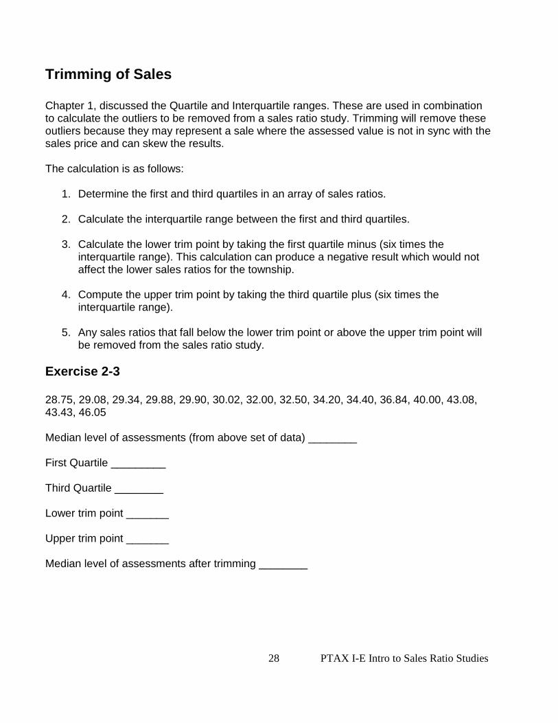
Trimming of Sales Chapter 1, discussed the Quartile and Interquartile ranges. These are used in combination to calculate the outliers to be removed from a sales ratio study. Trimming will remove these outliers because they may represent a sale where the assessed value is not in sync with the sales price and can skew the results. The calculation is as follows:
1. Determine the first and third quartiles in an array of sales ratios.
2. Calculate the interquartile range between the first and third quartiles.
3. Calculate the lower trim point by taking the first quartile minus (six times the interquartile range). This calculation can produce a negative result which would not affect the lower sales ratios for the township.
4. Compute the upper trim point by taking the third quartile plus (six times the interquartile range).
5. Any sales ratios that fall below the lower trim point or above the upper trim point will be removed from the sales ratio study.
Exercise 2-3 28.75, 29.08, 29.34, 29.88, 29.90, 30.02, 32.00, 32.50, 34.20, 34.40, 36.84, 40.00, 43.08, 43.43, 46.05 Median level of assessments (from above set of data) ________ First Quartile _________ Third Quartile ________ Lower trim point _______ Upper trim point _______ Median level of assessments after trimming ________
29 PTAX I-E Intro to Sales Ratio Studies
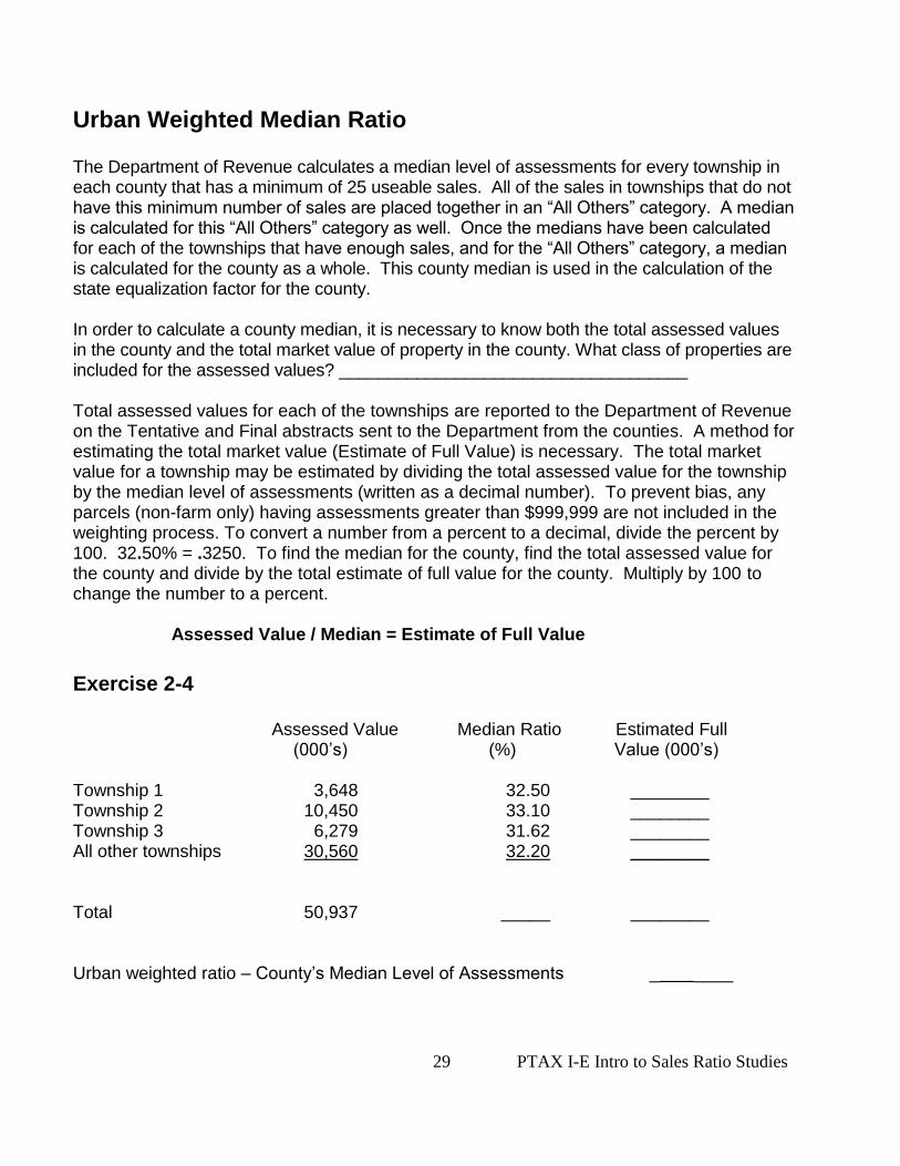
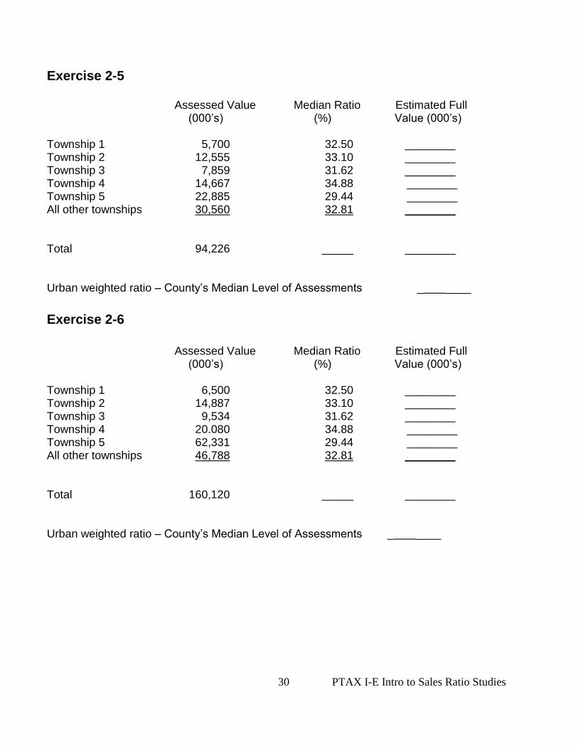
Urban Weighted Median Ratio The Department of Revenue calculates a median level of assessments for every township in each county that has a minimum of 25 useable sales. All of the sales in townships that do not have this minimum number of sales are placed together in an “All Others” category. A median is calculated for this “All Others” category as well. Once the medians have been calculated for each of the townships that have enough sales, and for the “All Others” category, a median is calculated for the county as a whole. This county median is used in the calculation of the state equalization factor for the county. In order to calculate a county median, it is necessary to know both the total assessed values in the county and the total market value of property in the county. What class of properties are included for the assessed values? ____________________________________ Total assessed values for each of the townships are reported to the Department of Revenue on the Tentative and Final abstracts sent to the Department from the counties. A method for estimating the total market value (Estimate of Full Value) is necessary. The total market value for a township may be estimated by dividing the total assessed value for the township by the median level of assessments (written as a decimal number). To prevent bias, any parcels (non-farm only) having assessments greater than $999,999 are not included in the weighting process. To convert a number from a percent to a decimal, divide the percent by 100. 32.50% = .3250. To find the median for the county, find the total assessed value for the county and divide by the total estimate of full value for the county. Multiply by 100 to change the number to a percent. Assessed Value / Median = Estimate of Full Value
Exercise 2-4 Assessed Value Median Ratio Estimated Full (000’s) (%) Value (000’s) Township 1 3,648 32.50 ________ Township 2 10,450 33.10 ________ Township 3 6,279 31.62 ________ All other townships 30,560 32.20 ________ Total 50,937 _____ ________ Urban weighted ratio – County’s Median Level of Assessments _ ____
30 PTAX I-E Intro to Sales Ratio Studies
Exercise 2-5 Assessed Value Median Ratio Estimated Full (000’s) (%) Value (000’s) Township 1 5,700 32.50 ________ Township 2 12,555 33.10 ________ Township 3 7,859 31.62 ________ Township 4 14,667 34.88 ________ Township 5 22,885 29.44 ________ All other townships 30,560 32.81 ________ Total 94,226 _____ ________ Urban weighted ratio – County’s Median Level of Assessments _ ____
Exercise 2-6
Assessed Value Median Ratio Estimated Full (000’s) (%) Value (000’s) Township 1 6,500 32.50 ________ Township 2 14,887 33.10 ________ Township 3 9,534 31.62 ________ Township 4 20.080 34.88 ________ Township 5 62,331 29.44 ________ All other townships 46,788 32.81 ________ Total 160,120 _____ ________ Urban weighted ratio – County’s Median Level of Assessments _ ____
31 PTAX I-E Intro to Sales Ratio Studies
Summary Each deed and assignment of beneficial interest of a land trust recorded must be accompanied by Form PTAX-203, Illinois Real Estate Transfer Declaration, unless specifically exempted under Section 31-45 of the Property Tax Code. The RETD is the primary source of information for conducting a sales ratio study.
If the sale involves land that is located in more than one township, the sale is excluded from the urban study.
Warranty deeds are acceptable if not rejected for some other reason. Trustee deeds are acceptable for the study if they pass all the edits. Corporate Warranty deeds are useable if the companies involved are not related.
When calculating the sales ratio, use the assessed value after the books are closed at the board of review divided by the net consideration from the sale price. The Sales Ratio Study provides the Median Level of Assessments for that jurisdiction for the year of the study. The year of the sales ratio study is the year from which the sales occurred. The median sales ratio is used:
1. In the computation of equalization multipliers. The sales ratio medians are the beginning point for the tentative multiplier.
2. In the review and appeal of assessments.
3. As a diagnostic tool to evaluate local assessment practices.
4. To determine eligibility for the assessor bonus award.
5. To determine eligibility for the reimbursement to the county of a portion of the salary of the Supervisor of Assessments.
Sales that do not meet the market value/arm’s length transaction criteria are excluded from the sales ratio study. The definition of market value is the most probable price which a property should bring in a competitive and open market under all conditions requisite to a fair sale, the buyer and seller each acting prudently and knowledgeably, and assuming the price is not affected by undue stimulus.
Verification of sales data for your jurisdiction should encompass all of the information placed on the PTAX 203 form by preparers, including date of instrument, parcel identification number and any other significant change that is attributable to the sale. Pay particular attention to the attributes that would identify a sale as an arm’s length transaction:
32 PTAX I-E Intro to Sales Ratio Studies
The buyer and seller are knowledgeable about the property
The buyer and seller are acting in their best interests
The property has been advertised on the market for a reasonable length of time o While a reasonable length of time can be a subjective attribute and that’s
because there is no definitive hard and fast rule guiding what is reasonable, the following lists the types of advertising considered acceptable with no discussion on the length of time:
Advertised via an MLS listing or with a Realtor Advertised by word of mouth Advertised by owner placing ‘For Sale’ sign in front yard Advertising via the internet
Provide the corrections, along with the required proof, for a sale to either be removed or added to the study to the CCAO’s office. The CCAO can forward the information to the Department when the review of the detail listing occurs. Trimming of outliers occurs to remove sales that do not have the assessments and the sales price in sync with each other, it is viewed that the sale does not represent an arm’s length transaction. Outliers are calculated using the formula from page 26. The Urban Weighted Ratio is used to calculate the County’s median level of assessments. It uses only non-farm sales transactions after the removal of parcels greater than $999,999 to prevent bias. The importance of this ratio is that it represents the beginning point for the calculation of the County’s multiplier factor to be applied to assessments for the following year and includes residential, other land/improvements, commercial and industrial classes of properties.
33 PTAX I-E Intro to Sales Ratio Studies
UNIT 2 Review Questions
1. T or F A sale of property between relatives will be included in the sales ratio
study.
2. T or F A sale for an exempt property will not be included in the sales ratio
study.
3. T or F The median level of assessments is found by ranking sales ratios in
ascending order and locating middle result.
4. T or F A property has to be advertised with a realtor to be an arm’s length
transaction.
5. T or F To calculate the upper and lower trim points for an array of data, the
first step is to identify the first and second quartiles.
6. T or F The calculation for the county’s urban weighted sales ratio median
includes all classes of property.
7. What are some of the uses for the sales ratio study?
_________________________________________________________________
_________________________________________________________________
_________________________________________________________________
_________________________________________________________________
____________________________________________________________
8. If a house assessed at $74,250 recently sold for $198,000, the sales ratio is
_____________. Was the house (over, statutorily, or under) assessed?
9. The 2014 study would use sales from ________ and assessed values for these
same properties from _______.
10. List two deed types that would be included in the sales ratio study:
_________________________________________________________
_________________________________________________________
11. List five uses of property that would exclude a sale from the sales ratio study:
__________________________________________________________________
________________________________________________________
34 PTAX I-E Intro to Sales Ratio Studies
12. List two other reasons why a sale would be excluded from the sales ratio study.
_________________________________________________________
_________________________________________________________
35 PTAX 1-E Intro to Sales Ratio Studies
Unit 3
Measure for the Uniformity of Assessments This unit covers some of the measures of assessment uniformity – the Coefficient of Dispersion (COD), the Price-Related Differential (PRD), and the Coefficient of Concentration (COC) – with a particular emphasis on the Coefficient of Dispersion as the most commonly used measure of assessment uniformity. The purpose of this unit is to provide a basic understanding of the measures of uniformity, each of which considers uniformity from a different perspective. Taking the measures into consideration together yields a more complete picture of uniformity than would be possible with one measure alone.
Learning Objectives After completing this unit, you should be able to
utilize the median in calculating the measures of uniformity.
calculate the COD, the COC, and the PRD.
interpret the degree of assessment uniformity as indicated by the measures of uniformity.
Terms and Concepts
Coefficient of Concentration (COC)
Coefficient of Dispersion (COD)
Concentration
Differential
Price-Related Differential (PRD)
36 PTAX 1-E Intro to Sales Ratio Studies
Coefficient of Dispersion
The most commonly used statistical measure of uniformity is the Coefficient of Dispersion (COD). The COD provides a measure of the variation of individual assessment ratios around the median level of assessment. Higher CODs indicate that individual ratios vary widely from the median, and that properties are not uniformly assessed. This also indicates that the property tax burden is not fairly distributed among taxpayers in that particular region or jurisdiction. The following page shows by graph how the more uniform COD is displayed when compared with a COD that has more variance.
37 PTAX 1-E Intro to Sales Ratio Studies
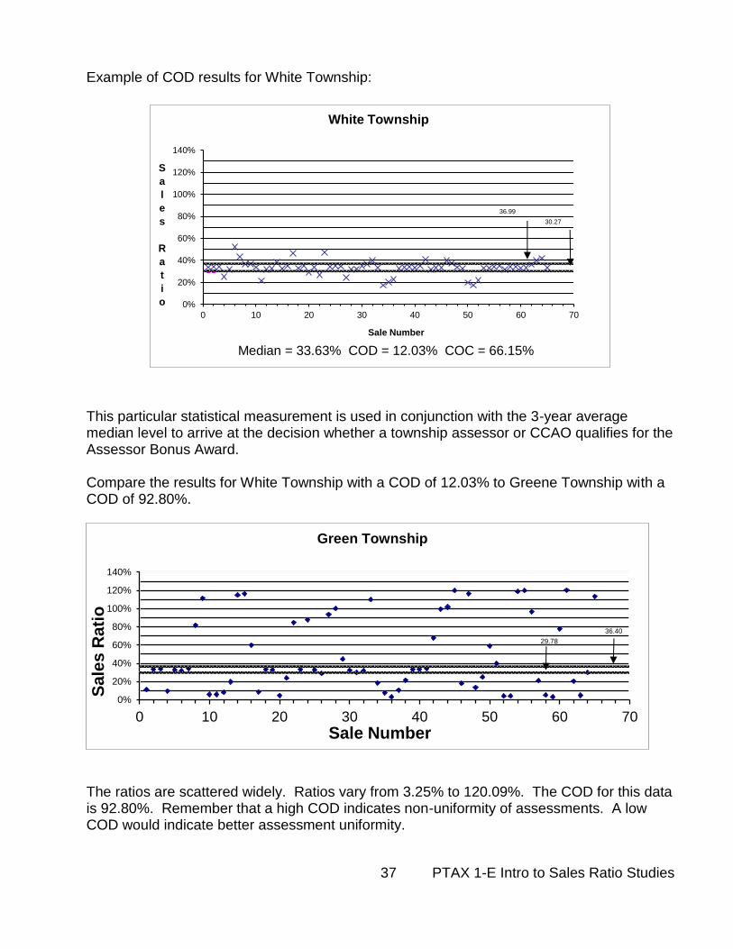
Example of COD results for White Township:
This particular statistical measurement is used in conjunction with the 3-year average median level to arrive at the decision whether a township assessor or CCAO qualifies for the Assessor Bonus Award. Compare the results for White Township with a COD of 12.03% to Greene Township with a COD of 92.80%.
The ratios are scattered widely. Ratios vary from 3.25% to 120.09%. The COD for this data is 92.80%. Remember that a high COD indicates non-uniformity of assessments. A low COD would indicate better assessment uniformity.
29.78
36.40
0%
20%
40%
60%
80%
100%
120%
140%
0 10 20 30 40 50 60 70
Sa
les
Ra
tio
Sale Number
Green Township
30.27
36.99
0%
20%
40%
60%
80%
100%
120%
140%
0 10 20 30 40 50 60 70
S
a
l
e
s
R
a
t
i
o
Sale Number
White Township
Median = 33.63% COD = 12.03% COC = 66.15% COV =
38 PTAX 1-E Intro to Sales Ratio Studies
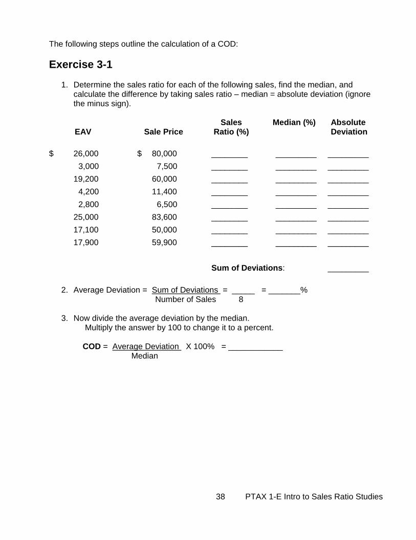
The following steps outline the calculation of a COD:
Exercise 3-1
1. Determine the sales ratio for each of the following sales, find the median, and calculate the difference by taking sales ratio – median = absolute deviation (ignore the minus sign).
Sales Median (%) Absolute EAV Sale Price Ratio (%) Deviation
$ 26,000 $ 80,000 ________ _________ _________
3,000 7,500 ________ _________ _________
19,200 60,000 ________ _________ _________
4,200 11,400 ________ _________ _________
2,800 6,500 ________ _________ _________
25,000 83,600 ________ _________ _________
17,100 50,000 ________ _________ _________
17,900 59,900 ________ _________ _________
Sum of Deviations: _________
2. Average Deviation = Sum of Deviations = _____ = _______%
Number of Sales 8
3. Now divide the average deviation by the median. Multiply the answer by 100 to change it to a percent. COD = Average Deviation X 100% = ____________
Median
39 PTAX 1-E Intro to Sales Ratio Studies
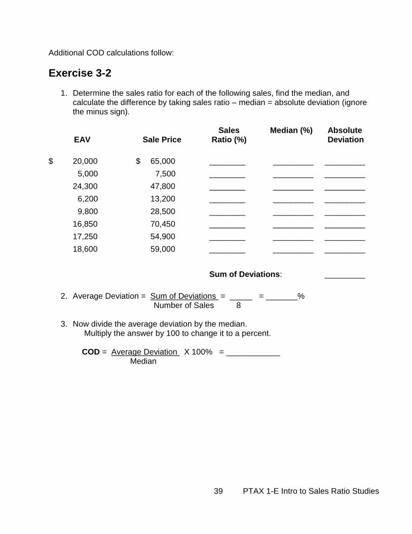
Additional COD calculations follow:
Exercise 3-2
1. Determine the sales ratio for each of the following sales, find the median, and calculate the difference by taking sales ratio – median = absolute deviation (ignore the minus sign).
Sales Median (%) Absolute EAV Sale Price Ratio (%) Deviation
$ 20,000 $ 65,000 ________ _________ _________
5,000 7,500 ________ _________ _________
24,300 47,800 ________ _________ _________
6,200 13,200 ________ _________ _________
9,800 28,500 ________ _________ _________
16,850 70,450 ________ _________ _________
17,250 54,900 ________ _________ _________
18,600 59,000 ________ _________ _________
Sum of Deviations: _________
2. Average Deviation = Sum of Deviations = _____ = _______%
Number of Sales 8
3. Now divide the average deviation by the median. Multiply the answer by 100 to change it to a percent. COD = Average Deviation X 100% = ____________
Median
40 PTAX 1-E Intro to Sales Ratio Studies
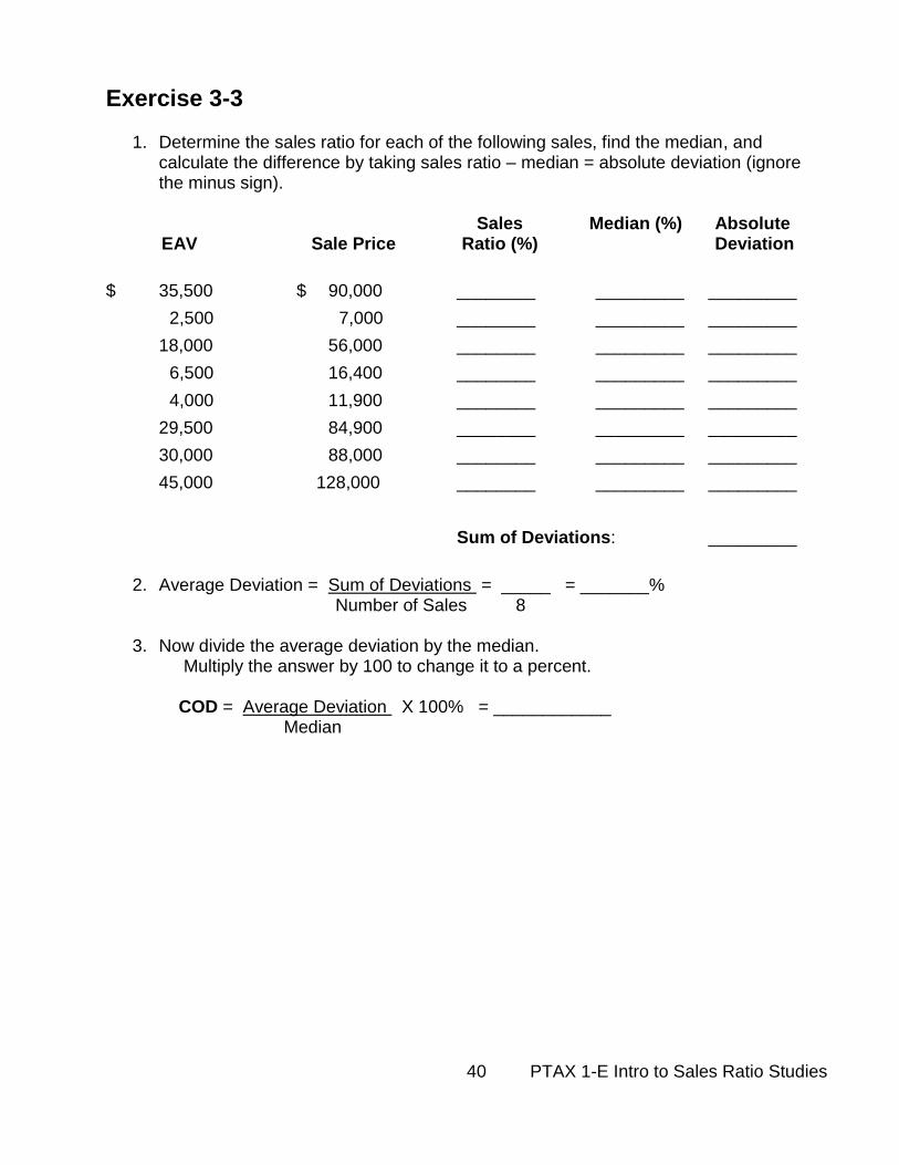
Exercise 3-3
1. Determine the sales ratio for each of the following sales, find the median, and calculate the difference by taking sales ratio – median = absolute deviation (ignore the minus sign).
Sales Median (%) Absolute EAV Sale Price Ratio (%) Deviation
$ 35,500 $ 90,000 ________ _________ _________
2,500 7,000 ________ _________ _________
18,000 56,000 ________ _________ _________
6,500 16,400 ________ _________ _________
4,000 11,900 ________ _________ _________
29,500 84,900 ________ _________ _________
30,000 88,000 ________ _________ _________
45,000 128,000 ________ _________ _________
Sum of Deviations: _________
2. Average Deviation = Sum of Deviations = _____ = _______%
Number of Sales 8
3. Now divide the average deviation by the median. Multiply the answer by 100 to change it to a percent. COD = Average Deviation X 100% = ____________
Median
41 PTAX 1-E Intro to Sales Ratio Studies
Exercise 3-4
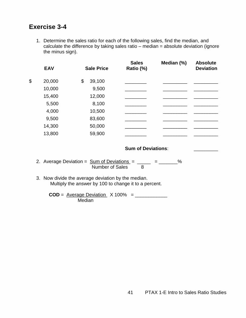
1. Determine the sales ratio for each of the following sales, find the median, and calculate the difference by taking sales ratio – median = absolute deviation (ignore the minus sign).
Sales Median (%) Absolute EAV Sale Price Ratio (%) Deviation
$ 20,000 $ 39,100 ________ _________ _________
10,000 9,500 ________ _________ _________
15,400 12,000 ________ _________ _________
5,500 8,100 ________ _________ _________
4,000 10,500 ________ _________ _________
9,500 83,600 ________ _________ _________
14,300 50,000 ________ _________ _________
13,800 59,900 ________ _________ _________
Sum of Deviations: _________
2. Average Deviation = Sum of Deviations = _____ = _______%
Number of Sales 8
3. Now divide the average deviation by the median. Multiply the answer by 100 to change it to a percent. COD = Average Deviation X 100% = ____________
Median
42 PTAX 1-E Intro to Sales Ratio Studies
Coefficient of Concentration
The Coefficient of Concentration (COC) measures assessment uniformity in a different way. The COC measures the percent of the ratios within a specific percentage range of the median. In many instances, a significant COC will measure the percent of ratios within 10% of the median ratio. The Department of Revenue uses a 10% range. If ratios are grouped closely (within 10%) of the median, the concentration of sales ratios will be large. A high COC indicates greater assessment uniformity than a low COC. The COD calculates how far the average deviation is from the median. With the COC the distance from the median is pre-determined at 10%. The COC yields the proportion of the ratios that fall within this range. The COC will be a number between 0% and 100%. A COC of 100% would indicate that all of the sales ratios are within 10% of the median. STEPS FOR CALCULATING THE COC: Step 1. Find the median sales ratio.
Step 2. Find the number which is 10% below the median
by multiplying the median ratio by .9. (100% -10% = 90% = .90 = .9)
Step 3. Find the number which is 10% above the median
by multiplying the median ratio by 1.1. (100% + 10% = 110% = 1.10 = 1.1)
Step 4. Count the number of ratios between the high
and low values computed in steps 2 and 3.
Step 5. Divide the number of ratios from step 4 by the total number of sales ratios and multiply by 100%.
What is the COC for the sets of sales ratios for Exercises 1 through 4 on the previous
pages?
Exercise 3-1 ___________
Exercise 3-2 ___________
Exercise 3-3 ___________
Exercise 3-4 ___________
43 PTAX 1-E Intro to Sales Ratio Studies
Unlike the COD, the COC has the advantage of not being affected by very high or very low ratios. The COC indicates only how concentrated the ratios are near the median ratio, but says nothing about the ratios outside the percentage range. Unlike the COD, a higher COC is an indicator of better assessment equity.
44 PTAX 1-E Introduction to Sales Ratio Studies
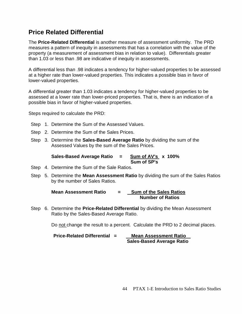
Price Related Differential
The Price-Related Differential is another measure of assessment uniformity. The PRD measures a pattern of inequity in assessments that has a correlation with the value of the property (a measurement of assessment bias in relation to value). Differentials greater than 1.03 or less than .98 are indicative of inequity in assessments. A differential less than .98 indicates a tendency for higher-valued properties to be assessed at a higher rate than lower-valued properties. This indicates a possible bias in favor of lower-valued properties. A differential greater than 1.03 indicates a tendency for higher-valued properties to be assessed at a lower rate than lower-priced properties. That is, there is an indication of a possible bias in favor of higher-valued properties. Steps required to calculate the PRD: Step 1. Determine the Sum of the Assessed Values.
Step 2. Determine the Sum of the Sales Prices.
Step 3. Determine the Sales-Based Average Ratio by dividing the sum of the Assessed Values by the sum of the Sales Prices. Sales-Based Average Ratio = Sum of AV's x 100% Sum of SP's
Step 4. Determine the Sum of the Sale Ratios.
Step 5. Determine the Mean Assessment Ratio by dividing the sum of the Sales Ratios by the number of Sales Ratios. Mean Assessment Ratio = Sum of the Sales Ratios Number of Ratios
Step 6. Determine the Price-Related Differential by dividing the Mean Assessment
Ratio by the Sales-Based Average Ratio. Do not change the result to a percent. Calculate the PRD to 2 decimal places.
Price-Related Differential = Mean Assessment Ratio
Sales-Based Average Ratio
45 PTAX 1-E Introduction to Sales Ratio Studies
Using the same set of sales from Page 38-41, calculate the PRD. What is the result? Exercise 3-1 ___________ Exercise 3-2 ___________ Exercise 3-3 ___________ Exercise 3-4 ___________ Use the area below as scratch paper.
46 PTAX 1-E Introduction to Sales Ratio Studies
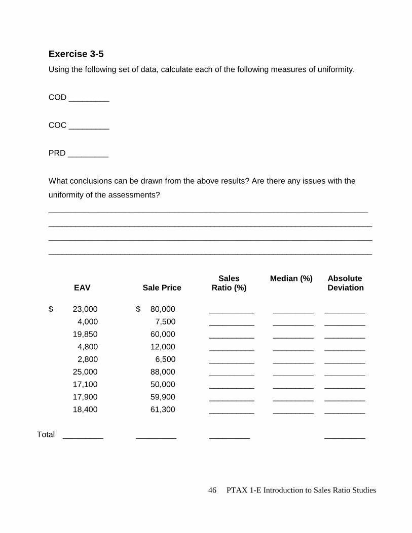
Exercise 3-5
Using the following set of data, calculate each of the following measures of uniformity.
COD _________
COC _________
PRD _________
What conclusions can be drawn from the above results? Are there any issues with the
uniformity of the assessments?
_______________________________________________________________________
________________________________________________________________________
________________________________________________________________________
________________________________________________________________________
Sales Median (%) Absolute EAV Sale Price Ratio (%) Deviation
$ 23,000 $ 80,000 __________ _________ _________
4,000 7,500 __________ _________ _________
19,850 60,000 __________ _________ _________
4,800 12,000 __________ _________ _________
2,800 6,500 __________ _________ _________
25,000 88,000 __________ _________ _________
17,100 50,000 __________ _________ _________
17,900 59,900 __________ _________ _________
18,400 61,300 __________ _________ _________
Total _________ _________ _________ _________
47 PTAX 1-E Introduction to Sales Ratio Studies
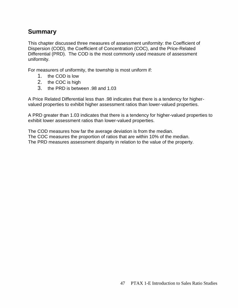
Summary
This chapter discussed three measures of assessment uniformity: the Coefficient of Dispersion (COD), the Coefficient of Concentration (COC), and the Price-Related Differential (PRD). The COD is the most commonly used measure of assessment uniformity. For measurers of uniformity, the township is most uniform if:
1. the COD is low
2. the COC is high
3. the PRD is between .98 and 1.03 A Price Related Differential less than .98 indicates that there is a tendency for higher-valued properties to exhibit higher assessment ratios than lower-valued properties. A PRD greater than 1.03 indicates that there is a tendency for higher-valued properties to exhibit lower assessment ratios than lower-valued properties. The COD measures how far the average deviation is from the median. The COC measures the proportion of ratios that are within 10% of the median. The PRD measures assessment disparity in relation to the value of the property.
48 PTAX 1-E Introduction to Sales Ratio Studies
UNIT 3 Review Questions 1. T or F Individual sales that are clustered around a township’s median indicates a
high COD result. 2. T or F A lower COC result indicates an issue with uniformity assessment.
3. T or F A PRD of 1.05 indicates a bias for assessments of higher-valued properties to be assessed higher than lower-valued properties.
4. Calculate the COD, COC and PRD for the following set of data:
Assessed Sales Sales Value Price Ratio Ranked Median Deviation
$ 4,000 16,000 25.00 21.15
2,000 7,600 26.32 22.22
13,000 32,000 40.63 24.82
8,000 29,500
5,000 18,800 26.32
3,500 14,100
14,700 35,800 41.06 26.60
2,200 10,400 21.15 26.67
8,000 30,000 26.67
2,200 9,900
19,400 54,000 30.51
8,700 31,000 28.06 31.09
8,300 26,700 31.09
3,600 11,800
19,500 47,300 41.23 40.31
9,700 23,200 40.63
3,100 7,500 41.06
18,500 45,900 40.31 41.23
12,000 25,000 48.00
20,000 52,700 37.95
4,100 8,000 48.00
25,200 51,700 48.08
5,000 10,400 48.08 48.74
13,300 50,000 26.60
______ ___________ ________
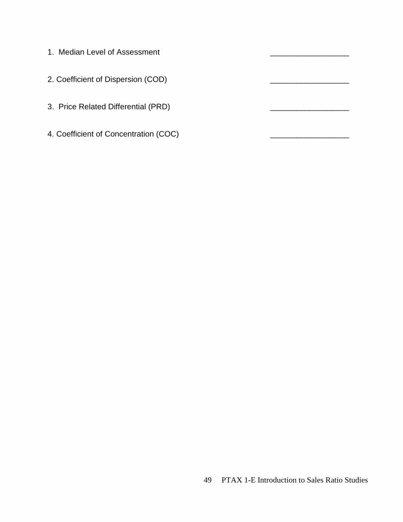
49 PTAX 1-E Introduction to Sales Ratio Studies
1. Median Level of Assessment __________________
2. Coefficient of Dispersion (COD) __________________
3. Price Related Differential (PRD) __________________
4. Coefficient of Concentration (COC) __________________
50 PTAX 1-E Introduction to Sales Ratio Studies
Unit 4 Equalization This unit covers various aspects of equalization including the definition of equalization, the three-year average median levels of assessments, and the effect of equalization. Also included is a brief mention of reassessment factors and their impact on the median levels of assessment used in calculating the equalization factor. The purpose of this unit is to provide a basic understanding of the equalization process and the correct uses for the equalization multipliers. The focus is on the procedures involved in the calculation of the equalization multiplier. LEARNING OBJECTIVES: After completing the assigned readings, you should be able to:
determine whether an objective is being met by the use of an equalization factor
calculate the three-year average median level of assessments
calculate the appropriate equalization factor using the three-year average median
meet the statutory conditions to determine the equalization factor
apply the equalization factor to individual properties TERMS AND CONCEPTS:
Average medians
Equalized Assessed Value (EAV)
Equalization
Reassessment factors
Township Assessor (TA)
51 PTAX 1-E Introduction to Sales Ratio Studies
Equalization is the application of a uniform percentage increase or decrease to assessed
values of various geographic areas or classes of property to bring assessments, on the
average, to a uniform level of market value.
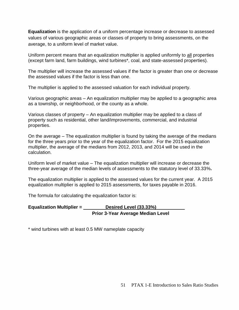
Uniform percent means that an equalization multiplier is applied uniformly to all properties (except farm land, farm buildings, wind turbines*, coal, and state-assessed properties). The multiplier will increase the assessed values if the factor is greater than one or decrease the assessed values if the factor is less than one. The multiplier is applied to the assessed valuation for each individual property. Various geographic areas – An equalization multiplier may be applied to a geographic area as a township, or neighborhood, or the county as a whole. Various classes of property – An equalization multiplier may be applied to a class of property such as residential, other land/improvements, commercial, and industrial properties. On the average – The equalization multiplier is found by taking the average of the medians for the three years prior to the year of the equalization factor. For the 2015 equalization multiplier, the average of the medians from 2012, 2013, and 2014 will be used in the calculation. Uniform level of market value – The equalization multiplier will increase or decrease the three-year average of the median levels of assessments to the statutory level of 33.33%. The equalization multiplier is applied to the assessed values for the current year. A 2015 equalization multiplier is applied to 2015 assessments, for taxes payable in 2016. The formula for calculating the equalization factor is:
Equalization Multiplier = Desired Level (33.33%)
Prior 3-Year Average Median Level * wind turbines with at least 0.5 MW nameplate capacity
52 PTAX 1-E Introduction to Sales Ratio Studies
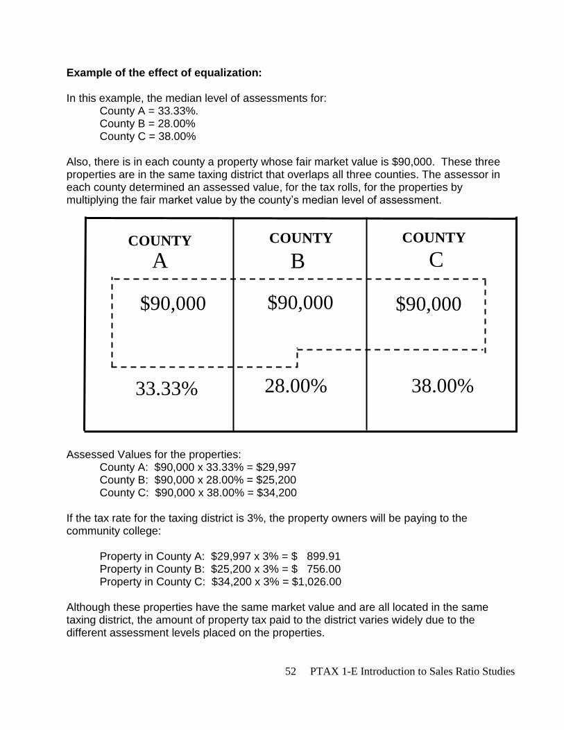
Example of the effect of equalization: In this example, the median level of assessments for:
County A = 33.33%. County B = 28.00% County C = 38.00%
Also, there is in each county a property whose fair market value is $90,000. These three properties are in the same taxing district that overlaps all three counties. The assessor in each county determined an assessed value, for the tax rolls, for the properties by multiplying the fair market value by the county’s median level of assessment.
Assessed Values for the properties:
County A: $90,000 x 33.33% = $29,997 County B: $90,000 x 28.00% = $25,200 County C: $90,000 x 38.00% = $34,200
If the tax rate for the taxing district is 3%, the property owners will be paying to the community college:
Property in County A: $29,997 x 3% = $ 899.91 Property in County B: $25,200 x 3% = $ 756.00 Property in County C: $34,200 x 3% = $1,026.00
Although these properties have the same market value and are all located in the same taxing district, the amount of property tax paid to the district varies widely due to the different assessment levels placed on the properties.
COUNTY COUNTY COUNTY
A B C
$90,000 $90,000 $90,000
33.33% 28.00% 38.00%
53 PTAX 1-E Introduction to Sales Ratio Studies
Each of the counties decides to apply an equalization multiplier. This multiplier is found by dividing 33.33% (the statutory level) by the average of the median levels of assessments for the prior 3 years.
Equalization Multiplier = Desired Level (33.33%)
Prior 3-Year Average Median Level
If the medians were the same for each of the prior three years as for the current year, the equalization factors would be:
County A: 33.33% = 1.0000 33.33%
County B: 33.33% = 1.1904 28.00%
County C: 33.33% = .8771 38.00%
Each county applies its equalization multiplier to all property in the county, except farm, coal, wind turbines over .5 MW capacity, and state-assessed properties. The equalized assessed value for the properties in the example will be:
County A: $29,997 x 1.0000 = $29,997 County B: $25,200 x 1.1904 = $29,998 County C: $34,200 x .8771 = $29,997
When the tax rate is applied to each of these three properties that were assessed at the median level of assessments and then equalized, the taxes owed will be the same.
Note: This example makes some special assumptions in order to illustrate the purpose of equalization. The example assumes 1) that the market values of the three properties were known to be the same, 2) that each of these properties were assessed at the median level of assessments for the county, and 3) that the medians for each of the counties were the same for the current year as for the prior 3 years.
54 PTAX 1-E Introduction to Sales Ratio Studies
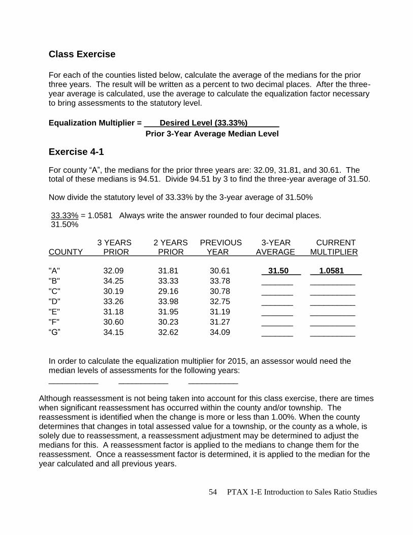
Class Exercise For each of the counties listed below, calculate the average of the medians for the prior three years. The result will be written as a percent to two decimal places. After the three-year average is calculated, use the average to calculate the equalization factor necessary to bring assessments to the statutory level.
Equalization Multiplier = Desired Level (33.33%)_______
Prior 3-Year Average Median Level
Exercise 4-1 For county “A”, the medians for the prior three years are: 32.09, 31.81, and 30.61. The total of these medians is 94.51. Divide 94.51 by 3 to find the three-year average of 31.50. Now divide the statutory level of 33.33% by the 3-year average of 31.50% 33.33% = 1.0581 Always write the answer rounded to four decimal places. 31.50% 3 YEARS 2 YEARS PREVIOUS 3-YEAR CURRENT COUNTY PRIOR PRIOR YEAR AVERAGE MULTIPLIER "A" 32.09 31.81 30.61 31.50 1.0581
"B" 34.25 33.33 33.78 _______ __________
"C" 30.19 29.16 30.78 _______ __________
"D" 33.26 33.98 32.75 _______ __________
"E" 31.18 31.95 31.19 _______ __________
"F" 30.60 30.23 31.27 _______ __________
“G” 34.15 32.62 34.09 _______ __________
In order to calculate the equalization multiplier for 2015, an assessor would need the median levels of assessments for the following years: ___________ ___________ ___________
Although reassessment is not being taken into account for this class exercise, there are times when significant reassessment has occurred within the county and/or township. The reassessment is identified when the change is more or less than 1.00%. When the county determines that changes in total assessed value for a township, or the county as a whole, is solely due to reassessment, a reassessment adjustment may be determined to adjust the medians for this. A reassessment factor is applied to the medians to change them for the reassessment. Once a reassessment factor is determined, it is applied to the median for the year calculated and all previous years.
55 PTAX 1-E Introduction to Sales Ratio Studies
Since the equalization multiplier uses the medians only for the prior three years, it is not necessary to carry the reassessment factor back beyond the three years. The reassessment factor is noted as a percent increase or decrease (denoted by a + or – sign). To find the actual multiplier to be applied, add or subtract the factor from 100% and change to a decimal number. Then multiply the median by all of the factors through all of the Supervisor of Assessments and Board of Review changes. If a factor is 0.00%, multiply by 1.
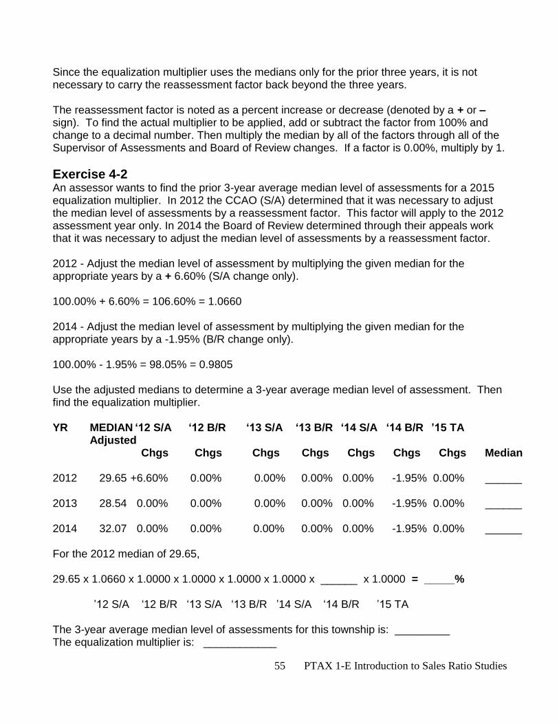
Exercise 4-2
An assessor wants to find the prior 3-year average median level of assessments for a 2015 equalization multiplier. In 2012 the CCAO (S/A) determined that it was necessary to adjust the median level of assessments by a reassessment factor. This factor will apply to the 2012 assessment year only. In 2014 the Board of Review determined through their appeals work that it was necessary to adjust the median level of assessments by a reassessment factor. 2012 - Adjust the median level of assessment by multiplying the given median for the appropriate years by a + 6.60% (S/A change only). 100.00% + 6.60% = 106.60% = 1.0660 2014 - Adjust the median level of assessment by multiplying the given median for the appropriate years by a -1.95% (B/R change only). 100.00% - 1.95% = 98.05% = 0.9805 Use the adjusted medians to determine a 3-year average median level of assessment. Then find the equalization multiplier. YR MEDIAN ‘12 S/A ‘12 B/R ‘13 S/A ‘13 B/R ‘14 S/A ‘14 B/R ’15 TA Adjusted Chgs Chgs Chgs Chgs Chgs Chgs Chgs Median 2012 29.65 +6.60% 0.00% 0.00% 0.00% 0.00% -1.95% 0.00% ______ 2013 28.54 0.00% 0.00% 0.00% 0.00% 0.00% -1.95% 0.00% ______ 2014 32.07 0.00% 0.00% 0.00% 0.00% 0.00% -1.95% 0.00% ______ For the 2012 median of 29.65, 29.65 x 1.0660 x 1.0000 x 1.0000 x 1.0000 x 1.0000 x ______ x 1.0000 = _____% ’12 S/A ‘12 B/R ‘13 S/A ‘13 B/R ’14 S/A ‘14 B/R ’15 TA The 3-year average median level of assessments for this township is: _________ The equalization multiplier is: ____________
56 PTAX 1-E Introduction to Sales Ratio Studies
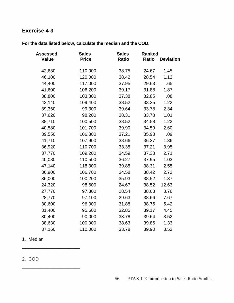
Exercise 4-3 For the data listed below, calculate the median and the COD.
Assessed Sales Sales Ranked Value Price Ratio Ratio Deviation
42,630 110,000 38.75 24.67 1.45
46,100 120,000 38.42 28.54 1.12
44,400 117,000 37.95 29.63 .65
41,600 106,200 39.17 31.88 1.87
38,800 103,800 37.38 32.85 .08
42,140 109,400 38.52 33.35 1.22
39,360 99,300 39.64 33.78 2.34
37,620 98,200 38.31 33.78 1.01
38,710 100,500 38.52 34.58 1.22
40,580 101,700 39.90 34.59 2.60
39,550 106,300 37.21 35.93 .09
41,710 107,900 38.66 36.27 1.36
36,920 110,700 33.35 37.21 3.95
37,770 109,200 34.59 37.38 2.71
40,080 110,500 36.27 37.95 1.03
47,140 118,300 39.85 38.31 2.55
36,900 106,700 34.58 38.42 2.72
36,000 100,200 35.93 38.52 1.37
24,320 98,600 24.67 38.52 12.63
27,770 97,300 28.54 38.63 8.76
28,770 97,100 29.63 38.66 7.67
30,600 96,000 31.88 38.75 5.42
31,400 95,600 32.85 39.17 4.45
30,400 90,000 33.78 39.64 3.52
38,630 100,000 38.63 39.85 1.33
37,160 110,000 33.78 39.90 3.52
1. Median
_________________
2. COD
_________________
57 PTAX 1-E Introduction to Sales Ratio Studies
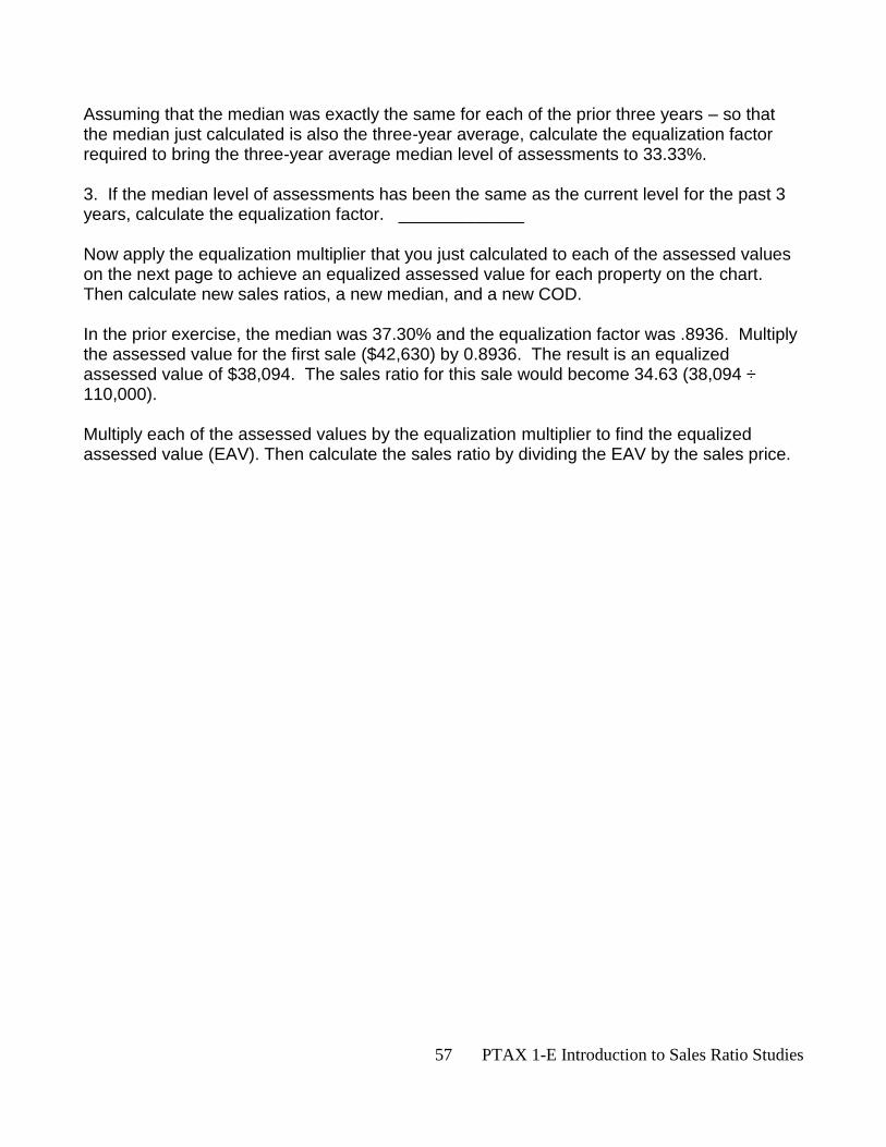
Assuming that the median was exactly the same for each of the prior three years – so that the median just calculated is also the three-year average, calculate the equalization factor required to bring the three-year average median level of assessments to 33.33%. 3. If the median level of assessments has been the same as the current level for the past 3 years, calculate the equalization factor. _____________ Now apply the equalization multiplier that you just calculated to each of the assessed values on the next page to achieve an equalized assessed value for each property on the chart. Then calculate new sales ratios, a new median, and a new COD. In the prior exercise, the median was 37.30% and the equalization factor was .8936. Multiply the assessed value for the first sale ($42,630) by 0.8936. The result is an equalized assessed value of $38,094. The sales ratio for this sale would become 34.63 (38,094 ÷ 110,000). Multiply each of the assessed values by the equalization multiplier to find the equalized assessed value (EAV). Then calculate the sales ratio by dividing the EAV by the sales price.
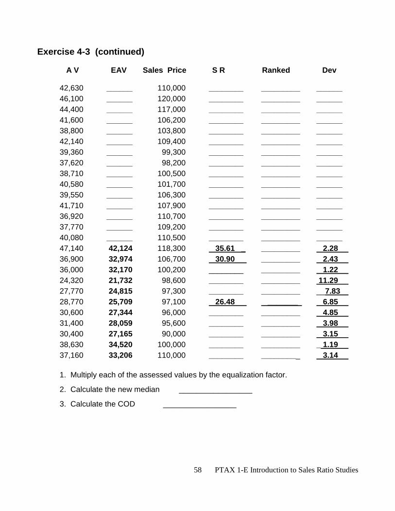
58 PTAX 1-E Introduction to Sales Ratio Studies
Exercise 4-3 (continued) A V EAV Sales Price S R Ranked Dev 42,630 ______ 110,000 ________ _________ ______
46,100 ______ 120,000 ________ _________ ______
44,400 ______ 117,000 ________ _________ ______
41,600 ______ 106,200 ________ _________ ______
38,800 ______ 103,800 ________ _________ ______
42,140 ______ 109,400 ________ _________ ______
39,360 ______ 99,300 ________ _________ ______
37,620 ______ 98,200 ________ _________ ______
38,710 ______ 100,500 ________ _________ ______
40,580 ______ 101,700 ________ _________ ______
39,550 ______ 106,300 ________ _________ ______
41,710 ______ 107,900 ________ _________ ______
36,920 ______ 110,700 ________ _________ ______
37,770 ______ 109,200 ________ _________ ______
40,080 ______ 110,500 ________ _________ ______
47,140 42,124 118,300 35.61 _ _________ 2.28
36,900 32,974 106,700 30.90 _________ 2.43
36,000 32,170 100,200 ________ _________ 1.22
24,320 21,732 98,600 ________ _________ 11.29
27,770 24,815 97,300 ________ _________ __7.83
28,770 25,709 97,100 26.48 _______ 6.85
30,600 27,344 96,000 ________ _________ 4.85
31,400 28,059 95,600 ________ _________ 3.98
30,400 27,165 90,000 ________ _________ 3.15
38,630 34,520 100,000 ________ _________ _ 1.19
37,160 33,206 110,000 ________ _________ 3.14
1. Multiply each of the assessed values by the equalization factor.
2. Calculate the new median _________________
3. Calculate the COD _________________
59 PTAX 1-E Introduction to Sales Ratio Studies
Summary Equalization is the application of a uniform percentage increase or decrease to assessed values of various geographic areas or classes of property to bring assessments, on the average, to a uniform level of market value.
In Illinois, the statutory level of assessments is 33 ⅓% of market value. Equalization multipliers adjust the three-year average median level of assessments to the statutory level.
The calculation of the equalization multiplier uses the average of the medians from the prior 3 years.
The formula for calculating the equalization multiplier is:
Equalization Multiplier = Desired Level (33.33%)
Prior 3-Year Average Median Level
The equalization multiplier is applied to the assessed values for the current year. A 2015 equalization multiplier is applied to 2015 assessments, taxes payable in 2016.
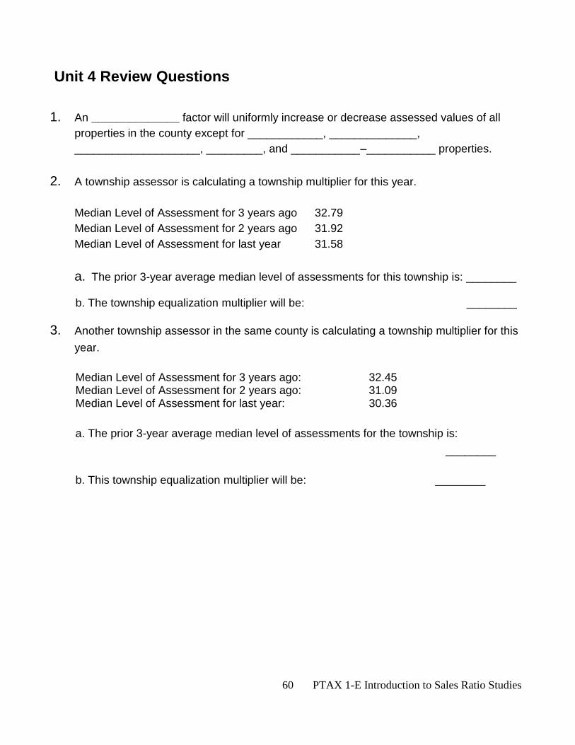
60 PTAX 1-E Introduction to Sales Ratio Studies
Unit 4 Review Questions
1. An ______________ factor will uniformly increase or decrease assessed values of all
properties in the county except for ____________, ______________,
____________________, _________, and ___________–___________ properties.
2. A township assessor is calculating a township multiplier for this year.
Median Level of Assessment for 3 years ago 32.79
Median Level of Assessment for 2 years ago 31.92
Median Level of Assessment for last year 31.58
a. The prior 3-year average median level of assessments for this township is: ________
b. The township equalization multiplier will be: ________
3. Another township assessor in the same county is calculating a township multiplier for this
year.
Median Level of Assessment for 3 years ago: 32.45 Median Level of Assessment for 2 years ago: 31.09 Median Level of Assessment for last year: 30.36
a. The prior 3-year average median level of assessments for the township is:
________
b. This township equalization multiplier will be: ________
61 PTAX 1-E Introduction to Sales Ratio Studies
Unit 5 Assessor Bonus This unit covers the qualifications and application procedure for the Assessor Bonus Award. This award is based on performance, using criteria with respect to the median level of assessments and uniformity of assessments as determined by the Coefficient of Dispersion. The purpose of this unit is to inform township assessors and supervisors of assessments of the availability of the Assessor Bonus award, highlighting the application process and eligibility. LEARNING OBJECTIVES: After completing the assigned readings, you should be able to:
realize that the bonus award is available to assessors
correctly complete an application for the bonus award
know which criteria applies to the assessor’s jurisdiction
determine whether eligibility criteria has been met for a given year TERMS AND CONCEPTS:
Elected County Official (ECO)
Illinois Municipal Retirement Fund (IMRF)
Tentative equalization factor
62 PTAX 1-E Introduction to Sales Ratio Studies
ASSESSOR BONUS AWARD
Any assessor, in counties other than Cook or the St. Clair County Assessor, may petition the Department of Revenue to receive additional compensation based on performance. In order to receive the assessor bonus award, you must
1. be in a qualifying position,
2. have a three-year average median within the correct range,
3. determine whether your jurisdiction is within a small or large county,
4. have a COD less than the COD requirement based on the size of your county, and
5. file a completed application within the correct time frame. 35 ILCS 200 Sec 4-20: “As used in this Section, ‘assessor’ means any township or multi-township assessor, or supervisor of assessments.” Positions that qualify for the bonus award are
1. any elected or appointed township or multi-township assessor, or 2. the supervisor of assessments. Positions that do not qualify for the bonus award include
1. township assessors in Cook county, 2. county assessors in Cook and St. Clair counties, 3. an individual who has contracted to complete the assessments, and 4. a deputy assessor. County assessors in Cook and St. Clair counties do not meet the condition of being in a qualified position since the requirement is for an individual to hold the title of a “supervisor of assessments.” An individual who has contracted to complete the assessments does not meet the condition as he or she does not hold the position of township assessor. The “Illinois County Populations Based on the 2010 Decennial Census Counts” from the US Department of Commerce, Bureau of the Census is the guide used to determine whether the assessor’s county is a small county (50,000 or fewer) or a large county (over 50,000).
63 PTAX 1-E Introduction to Sales Ratio Studies
In order to qualify for the bonus award, a person must meet the requirements listed below. For counties with 50,000 or fewer inhabitants, the requirements are: a three-year average level of assessments between 31.33% and 35.33% of the fair cash
value for the assessment jurisdiction, and a coefficient of dispersion (COD) no greater than 30.00 percent. For counties with more than 50,000 inhabitants, the requirements are: a three-year average level of assessments between 31.33% and 35.33% of the fair cash
value for the assessment jurisdiction, and a coefficient of dispersion (COD) no greater than 15.00 percent. Assessors may use the Department’s sales ratio data or the assessor’s own data with proper documentation. If the township does not have enough sales to have its own study done by the Department of Revenue, the township assessor may use independent appraisals and/or trending to establish the median level of assessments and the COD. File Form PTAX-205, Assessor’s Application for Additional Compensation, after you have signed your assessment books, but no later than 60 days after your county’s tentative equalization factor hearing for the assessment year. Do not submit Form PTAX-205 before your assessment books are given to the chief county assessment officer (CCAO) or board of review, as appropriate. Trending is a process whereby the sales from one year are combined with the sales from a prior or a following year in order to have enough sales (25) to complete a sales ratio study. By combining sales from 2 or 3 years, many townships will have enough sales to determine the median level of assessments. Trending may be used for intra-county equalization factors or for the assessor bonus award.
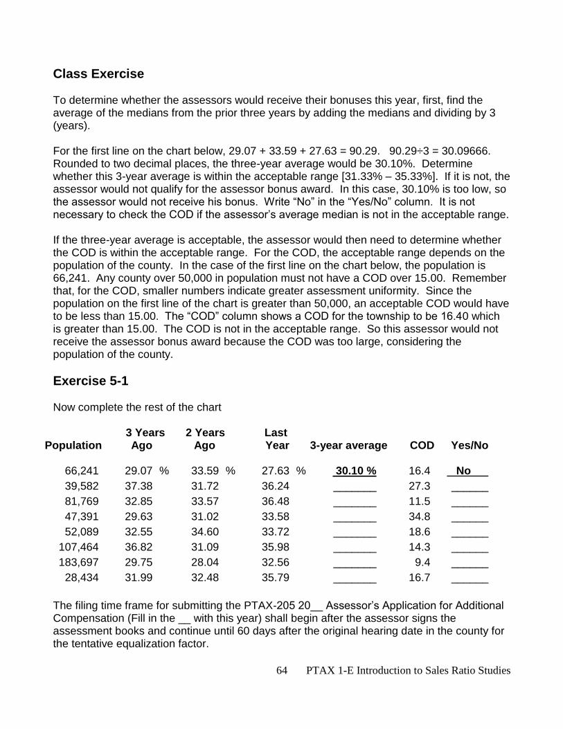
64 PTAX 1-E Introduction to Sales Ratio Studies
Class Exercise To determine whether the assessors would receive their bonuses this year, first, find the average of the medians from the prior three years by adding the medians and dividing by 3 (years). For the first line on the chart below, 29.07 + 33.59 + 27.63 = 90.29. 90.29÷3 = 30.09666. Rounded to two decimal places, the three-year average would be 30.10%. Determine whether this 3-year average is within the acceptable range [31.33% – 35.33%]. If it is not, the assessor would not qualify for the assessor bonus award. In this case, 30.10% is too low, so the assessor would not receive his bonus. Write “No” in the “Yes/No” column. It is not necessary to check the COD if the assessor’s average median is not in the acceptable range. If the three-year average is acceptable, the assessor would then need to determine whether the COD is within the acceptable range. For the COD, the acceptable range depends on the population of the county. In the case of the first line on the chart below, the population is 66,241. Any county over 50,000 in population must not have a COD over 15.00. Remember that, for the COD, smaller numbers indicate greater assessment uniformity. Since the population on the first line of the chart is greater than 50,000, an acceptable COD would have to be less than 15.00. The “COD” column shows a COD for the township to be 16.40 which is greater than 15.00. The COD is not in the acceptable range. So this assessor would not receive the assessor bonus award because the COD was too large, considering the population of the county.
Exercise 5-1 Now complete the rest of the chart 3 Years 2 Years Last
Population Ago Ago Year 3-year average COD Yes/No 66,241 29.07 % 33.59 % 27.63 % 30.10 % 16.4 No
39,582 37.38 31.72 36.24 _______ 27.3 ______
81,769 32.85 33.57 36.48 _______ 11.5 ______
47,391 29.63 31.02 33.58 _______ 34.8 ______
52,089 32.55 34.60 33.72 _______ 18.6 ______
107,464 36.82 31.09 35.98 _______ 14.3 ______
183,697 29.75 28.04 32.56 _______ 9.4 ______
28,434 31.99 32.48 35.79 _______ 16.7 ______
The filing time frame for submitting the PTAX-205 20__ Assessor’s Application for Additional Compensation (Fill in the __ with this year) shall begin after the assessor signs the assessment books and continue until 60 days after the original hearing date in the county for the tentative equalization factor.
65 PTAX 1-E Introduction to Sales Ratio Studies
An assessor may obtain a PTAX-205 form from the Supervisor of Assessments Instructions for completing the PTAX-205 Assessor’s Application for Additional Compensation
1. Be sure to check whether you contribute to the Illinois Municipal Retirement Fund (IMRF). If the answer is “Yes,” check whether it is “Regular” or “ECO.” “ECO” refers to Elected County Officials. However, check with the township or county office to determine which of these options applies to your office.
2. On line 6a, mark whether you are “elected,” “appointed,” or “on contract.”
3. Be sure to sign the form at the bottom of the front page.
4. File the application within the correct time frame: ”after you have signed your assessment books, but no later than 60 days after your county’s tentative equalization factor hearing for (the year of the application).”
If your jurisdiction does not have a minimum of 25 useable sales for any one, or more, of the three years, you may supplement the actual sales with independent appraisals or use a process for combining sales, from prior or subsequent years, called trending.
66 PTAX 1-E Introduction to Sales Ratio Studies
Summary The assessor bonus award is based on the performance of the assessor. Township and multi-township assessors and supervisors of assessments from all counties except Cook or St Clair County Assessor may qualify for the bonus award. Assessors must file an application for the bonus award after the assessment books are signed and within 60 days of the hearing date in their counties for the tentative multiplier. If the jurisdiction does not have a minimum of 25 useable sales for any one, or more, of the three years, you may supplement the actual sales with independent appraisals or use trending.
67 PTAX 1-E Introduction to Sales Ratio Studies
Unit 5 Review Questions
1. A township assessor is applying for the bonus award for this year. The COD is 15.92%. Median Level of Assessment for 3 years ago 32.79 Median Level of Assessment for 2 years ago 31.92 Median Level of Assessment for last year 31.58
a. If the population of the county is less than 50,000, will the assessor receive his or her bonus? ________
b. If the population of the county is greater than 50,000, will the assessor receive
his or her bonus? ________
2. A township assessor is applying for the bonus award for this year. The COD is 14.80%. Median Level of Assessment for 3 years ago: 32.45 Median Level of Assessment for 2 years ago: 31.09 Median Level of Assessment for last year: 30.36
a. If the population of the county is less than 50,000, will the assessor receive his or her bonus? ________
b. If the population of the county is greater than 50,000, will the assessor receive
his or her bonus? ________
3. In order to qualify for the assessor bonus award, the assessor must be in a __________ _________, have a _____- year average median level of assessments between ______ and _______, and a COD no greater than _____ (assuming that the population of the county is 50,000 or less).
68 PTAX 1-E Introduction to Sales Ratio Studies
Unit 6 Trending This unit covers the process of trending to combine sales from two or more years when there were not enough sales from a given year to conduct a separate sales ratio study for a township. The trending process adjusts the values of the sales from one year to current market conditions for the year that did not have enough sales to achieve a sales ratio study. The trended sales from one (or more) year(s) are then combined with the actual market sales from the year of the sales ratio study. Using the combined sales, a sales ratio may then be completed. The purpose of this unit is to familiarize you with the appropriate circumstances when trending may be used and the procedures necessary for the calculations. Learning Objectives: After completing the assigned readings, you should be able to
know what trending will accomplish
be familiar with the appropriate occasions when trending may or may not be used
be able to calculate a trending factor
use the trending factor in adjusting sales for current market values
complete a sales ratio study with the adjusted sales combined with current sales Terms and Concepts
adjusted sales prices
trending
trending factor
69 PTAX 1-E Introduction to Sales Ratio Studies
Need for Trended Medians
The prior 3-year average median level of assessments (adjusted for change, if applicable) is used in the: A. Process of determining equalization factor B. Qualifications for the Assessor's Bonus Award. The average of the medians from the prior three years must be between 31.33%
and 35.33%. (Note: The COD must also be in the correct range.)
Before a three-year average median level of assessments can be established, there must be enough useable sales within a jurisdiction to establish a median level of assessments for each of the years being used in the calculation.
For example, if a 2015 township multiplier is being calculated, a median level for 2012, 2013, and 2014 is used to determine the prior 3-year average median level of assessments for the assessment year of 2015. In order to calculate the 2015 township multiplier, the following information must be available: Median Sales Ratio for 2012 34.50 Median Sales Ratio for 2013 33.90 Median Sales Ratio for 2014 34.00 102.40 ÷ 3 = 34.13%
There must be a minimum of 25 useable sales and/or appraisals before an assessment district can implement a Sales Ratio Study. If an assessment district does not have 25 useable sales in a particular year, appraisals can be used to supplement this study. Properties must be randomly selected, and the appraisals performed by an independent appraiser. Counties may find the burden of hiring independent appraisers cumbersome and costly. An alternative to using independent appraisals is the process called trending.
33.33%
Prior 3-year average median
70 PTAX 1-E Introduction to Sales Ratio Studies
Trending may be used to determine a median level of assessments in the calculation of: 1. Intra-County Equalization 2. Assessor Bonus Award Trending is not used in the calculation of the state equalization multiplier. Trending is a method that may be used to determine a median level of assessments when one, or more than one, of the 3 years involved in finding the prior 3-year median level of assessments for the purposes listed above does not have 25 useable sales. In the technique of trending, the sales that pass the editing for a sales ratio study can be adjusted back in time or they may be adjusted forward in time. The new ratios are combined with the existing sales ratios of that year. A median level of assessments for the year in question can be established from the combined ratios. When trending, trend back first, if possible, since the sales are more current. If the median that is being established is for the most current of the 3 years, it will be necessary to trend forward. If the Supervisor of Assessments wanted to apply a township equalization multiplier for 2015, he would need the township medians for 2012, 2013, and 2014. If the township did not have enough sales to find a township median for 2014, he could trend the 2013 sales forward and calculate sales ratios using the adjusted market values (now 2014 market value) and the assessed values from 2013 to find 2014 sales ratios. Combine these ratios with the ratios found from the actual sales in 2014 to find a median for the township for 2014. Always use the assessed valuation for the year prior to the year of the sales ratio study. For a 2014 sales ratio study, the assessed values on the same properties that sold must come from 2013. Example 1: The Supervisor of Assessments plans to determine an equalization multiplier for the townships for 2015. He will need the medians for 2012, 2013, and 2014 in order to calculate the prior 3-year average median level of assessments. 2012 median = 29.78 2013 median = 30.07 2014 median = _______ The 2013 sales would be adjusted by a trending factor to 2014 values. New sales ratios would be calculated for the 2013 sales adjusted to 2014 market value. The sales ratios would be found by dividing the 2013 assessed value from the properties that sold by the adjusted 2014 market value of those same properties.
71 PTAX 1-E Introduction to Sales Ratio Studies
Example 2: The Board of Review plans to determine an equalization multiplier for the townships for 2015. They will need the medians for 2012, 2013, and 2014 in order to calculate the prior 3-year average median level of assessments. 2012 median = _______ 2013 median = 32.59 2014 median = 33.80 Since the missing median is the first of the three years, the 2013 sales would be trended backward. The 2013 sales would be adjusted by a trending factor to 2012 market values. New sales ratios would be calculated for the 2013 sales adjusted to 2012 market value. Sales ratios are found by dividing the prior year assessed value by the current year selling price. A 2012 sales ratio is found by dividing the 2011 assessed value by the 2012 sales price. Example 3: The Board of Review plans to determine an equalization multiplier for the townships for 2015. They will need the medians for 2012, 2013, and 2014 in order to calculate the prior 3-year average median level of assessments. In 2013 there were less than 25 sales. 2012 median = 28.72 2013 median = ______ 2014 median = 31.25 Since the missing median is the middle of the three years, the 2012 sales may be trended forward or the 2014 sales may be trended backward. If there is a choice, trend backward. In this case the 2014 sales would be adjusted by a trending factor to 2013 market values. The 2014 sales are trended backward to become 2013 sales. New sales ratios would be calculated for the 2014 sales adjusted to 2013 market value. A 2013 sales ratio is found by dividing the 2012 assessed value by the 2013 sales price. So, the sales ratios would be found by dividing the 2012 assessed value from the properties that sold (in 2014 adjusted backward to 2013 market value) by the adjusted 2013 market value of those same properties. If two or more years are missing, it may be necessary to trend one year forward and another year back or two years forward (backward) to achieve the 25 useable sales. The trending factor is the number that will be used to adjust the sales price (market value) of a property either forward to a later year or backward to an estimate of market value for a year previous to the actual year of sale.
72 PTAX 1-E Introduction to Sales Ratio Studies
The trending factor depends on the county’s medians to adjust the value from the value at the year of sale to an estimate of the value for the year that did not have enough sales. Trending Factor = County Median — Trended From Year County Median — Trended To Year

73 PTAX 1-E Introduction to Sales Ratio Studies
Exercise 6-1 Calculate the trending factors (to 4 decimal places) if a county’s urban-weighted medians are:
2012 2013 2014
31.57 30.48 32.95
1. Trend 2012 forward to 2013 Trending Factor = _________
2. Trend 2014 back to 2013 Trending Factor = _________
3. Trend 2013 back to 2012 Trending Factor = _________
4. Trend 2013 forward to 2014 Trending Factor = _________
Using the information from above exercise, determine from what year the assessed values would come.
1. Trend 2012 forward to 2013 Assessed Values from __________
2. Trend 2014 back to 2013 Assessed Values from __________
3. Trend 2013 back to 2012 Assessed Values from __________
4. Trend 2013 forward to 2014 Assessed Values from __________
74 PTAX 1-E Introduction to Sales Ratio Studies
Exercise 6-2 Calculate the trending factors (to 4 decimal places) if a county’s urban-weighted medians are:
2012 2013 2014
30.08 35.32 29.54
5. Trend 2012 forward to 2013 Trending Factor = _________
6. Trend 2014 back to 2013 Trending Factor = _________
7. Trend 2013 back to 2012 Trending Factor = _________
8. Trend 2013 forward to 2014 Trending Factor = _________
Using the information from above exercise, determine from what year the assessed values would come.
5. Trend 2012 forward to 2013 Assessed Values from __________
6. Trend 2014 back to 2013 Assessed Values from __________
7. Trend 2013 back to 2012 Assessed Values from __________
8. Trend 2013 forward to 2014 Assessed Values from __________
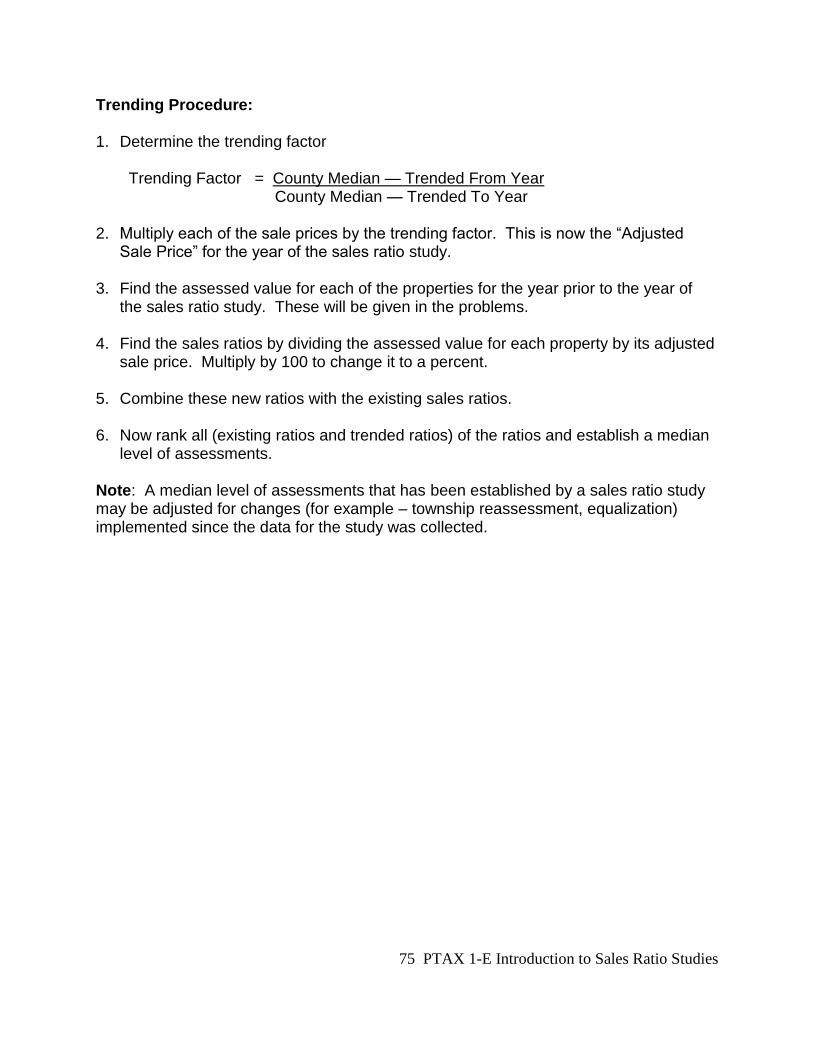
75 PTAX 1-E Introduction to Sales Ratio Studies
Trending Procedure: 1. Determine the trending factor
Trending Factor = County Median — Trended From Year County Median — Trended To Year
2. Multiply each of the sale prices by the trending factor. This is now the “Adjusted Sale Price” for the year of the sales ratio study.
3. Find the assessed value for each of the properties for the year prior to the year of the sales ratio study. These will be given in the problems.
4. Find the sales ratios by dividing the assessed value for each property by its adjusted sale price. Multiply by 100 to change it to a percent.
5. Combine these new ratios with the existing sales ratios.
6. Now rank all (existing ratios and trended ratios) of the ratios and establish a median level of assessments.
Note: A median level of assessments that has been established by a sales ratio study may be adjusted for changes (for example – township reassessment, equalization) implemented since the data for the study was collected.
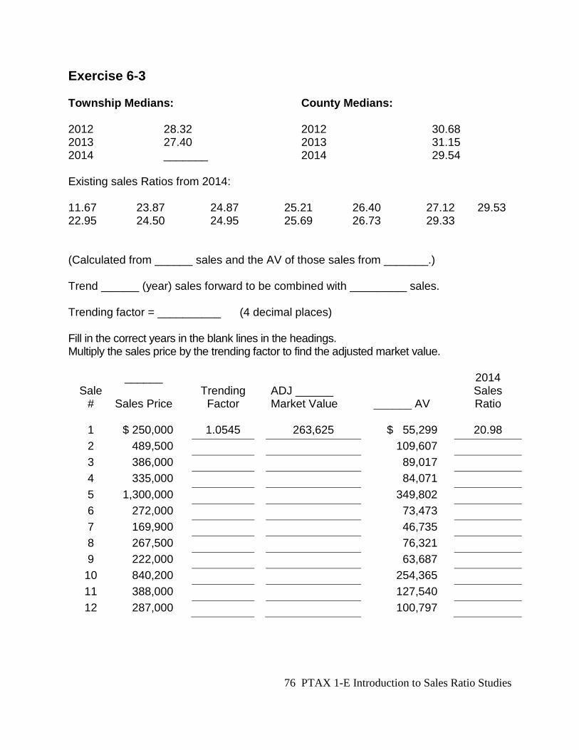
76 PTAX 1-E Introduction to Sales Ratio Studies
Exercise 6-3 Township Medians: County Medians: 2012 28.32 2012 30.68 2013 27.40 2013 31.15 2014 _______ 2014 29.54 Existing sales Ratios from 2014: 11.67 23.87 24.87 25.21 26.40 27.12 29.53 22.95 24.50 24.95 25.69 26.73 29.33 (Calculated from ______ sales and the AV of those sales from _______.) Trend ______ (year) sales forward to be combined with _________ sales. Trending factor = __________ (4 decimal places) Fill in the correct years in the blank lines in the headings. Multiply the sales price by the trending factor to find the adjusted market value.
______ 2014 Sale
# Sales Price Trending
Factor ADJ ______
Market Value ______ AV Sales
Ratio
1 $ 250,000 1.0545 263,625 $ 55,299 20.98
2 489,500 109,607
3 386,000 89,017
4 335,000 84,071
5 1,300,000 349,802
6 272,000 73,473
7 169,900 46,735
8 267,500 76,321
9 222,000 63,687
10 840,200 254,365
11 388,000 127,540
12 287,000 100,797
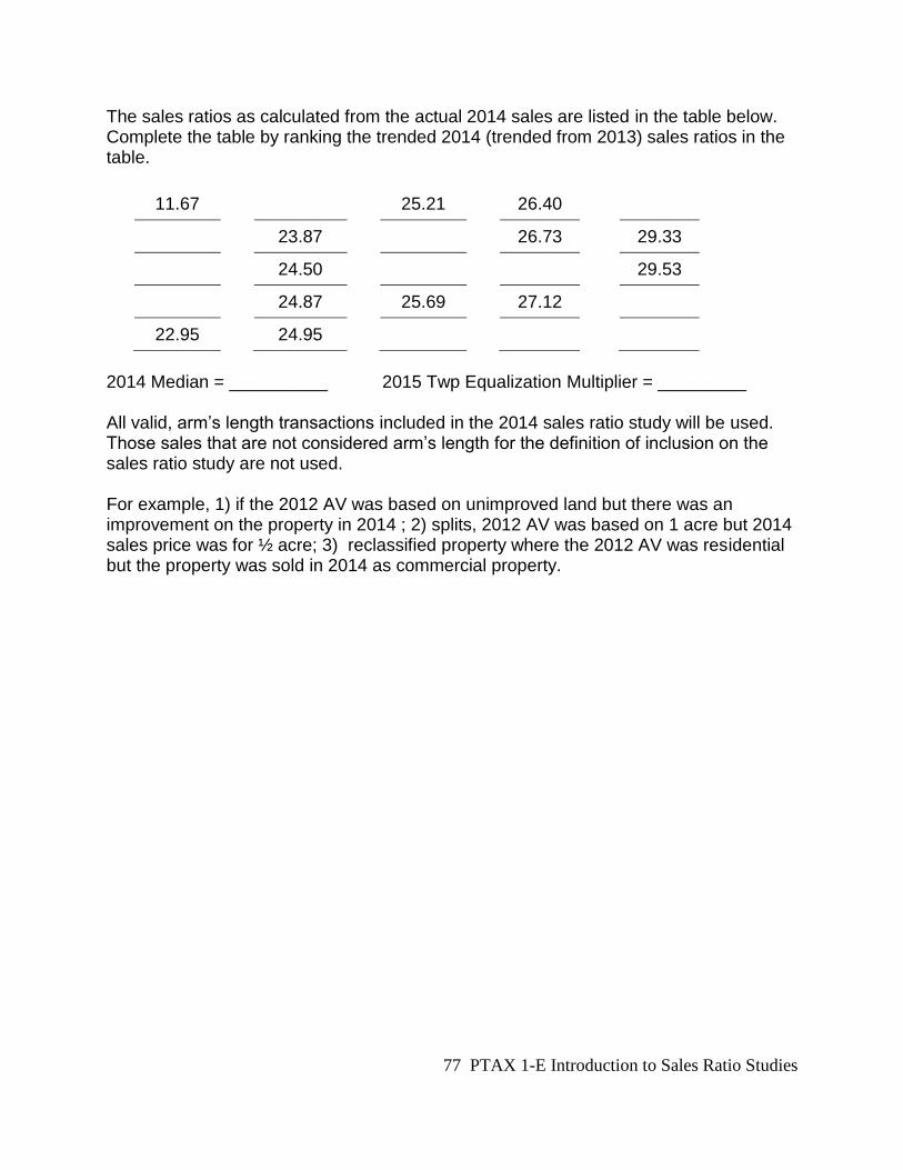
77 PTAX 1-E Introduction to Sales Ratio Studies
The sales ratios as calculated from the actual 2014 sales are listed in the table below. Complete the table by ranking the trended 2014 (trended from 2013) sales ratios in the table.
11.67 25.21 26.40
23.87 26.73 29.33
24.50 29.53
24.87 25.69 27.12
22.95 24.95
2014 Median = __________ 2015 Twp Equalization Multiplier = _________ All valid, arm’s length transactions included in the 2014 sales ratio study will be used. Those sales that are not considered arm’s length for the definition of inclusion on the sales ratio study are not used. For example, 1) if the 2012 AV was based on unimproved land but there was an improvement on the property in 2014 ; 2) splits, 2012 AV was based on 1 acre but 2014 sales price was for ½ acre; 3) reclassified property where the 2012 AV was residential but the property was sold in 2014 as commercial property.
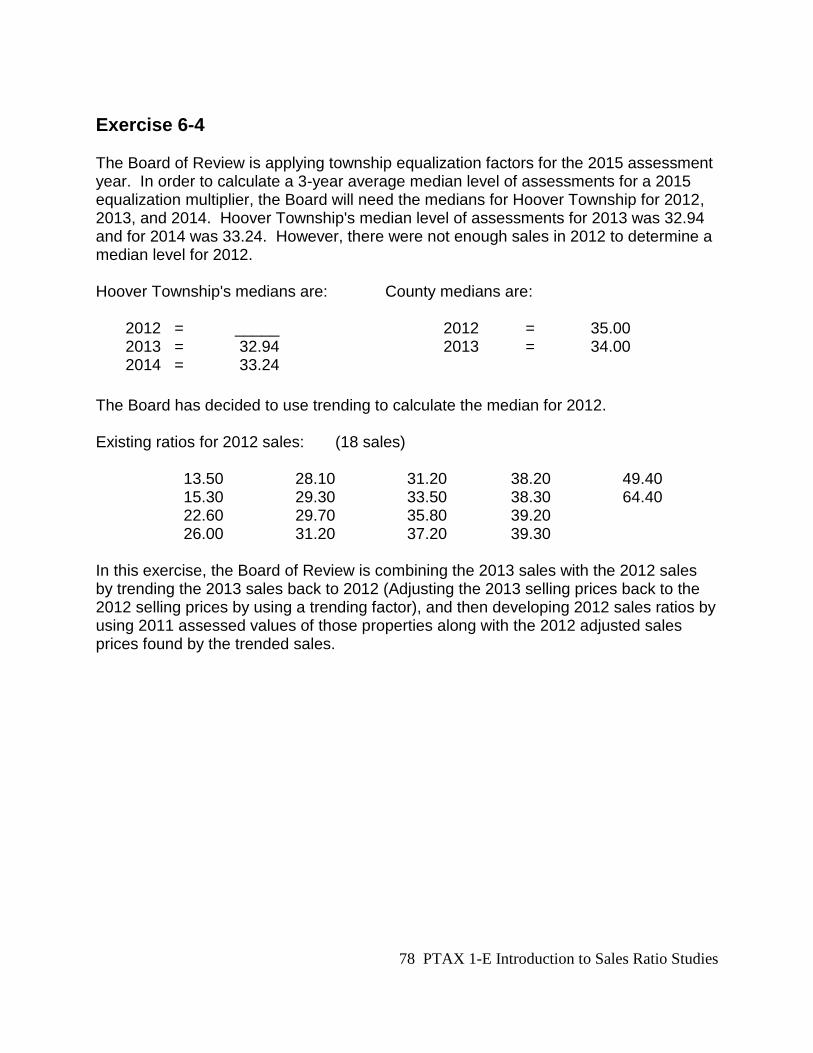
78 PTAX 1-E Introduction to Sales Ratio Studies
Exercise 6-4 The Board of Review is applying township equalization factors for the 2015 assessment year. In order to calculate a 3-year average median level of assessments for a 2015 equalization multiplier, the Board will need the medians for Hoover Township for 2012, 2013, and 2014. Hoover Township's median level of assessments for 2013 was 32.94 and for 2014 was 33.24. However, there were not enough sales in 2012 to determine a median level for 2012. Hoover Township's medians are: County medians are: 2012 = _____ 2012 = 35.00 2013 = 32.94 2013 = 34.00 2014 = 33.24
The Board has decided to use trending to calculate the median for 2012. Existing ratios for 2012 sales: (18 sales) 13.50 28.10 31.20 38.20 49.40 15.30 29.30 33.50 38.30 64.40 22.60 29.70 35.80 39.20 26.00 31.20 37.20 39.30 In this exercise, the Board of Review is combining the 2013 sales with the 2012 sales by trending the 2013 sales back to 2012 (Adjusting the 2013 selling prices back to the 2012 selling prices by using a trending factor), and then developing 2012 sales ratios by using 2011 assessed values of those properties along with the 2012 adjusted sales prices found by the trended sales.
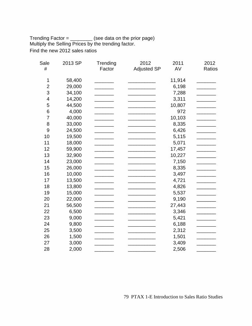
79 PTAX 1-E Introduction to Sales Ratio Studies
Trending Factor = ________ (see data on the prior page) Multiply the Selling Prices by the trending factor.
Find the new 2012 sales ratios
Sale 2013 SP Trending 2012 2011 2012 # Factor Adjusted SP AV Ratios 1 58,400 _______ __________ 11,914 _______
2 29,000 _______ __________ 6,198 _______
3 34,100 _______ __________ 7,288 _______
4 14,200 _______ __________ 3,311 _______
5 44,500 _______ __________ 10,807 _______
6 4,000 _______ __________ 972 _______
7 40,000 _______ __________ 10,103 _______
8 33,000 _______ __________ 8,335 _______
9 24,500 _______ __________ 6,426 _______
10 19,500 _______ __________ 5,115 _______
11 18,000 _______ __________ 5,071 _______
12 59,900 _______ __________ 17,457 _______
13 32,900 _______ __________ 10,227 _______
14 23,000 _______ __________ 7,150 _______
15 26,000 _______ __________ 8,335 _______
16 10,000 _______ __________ 3,497 _______
17 13,500 _______ __________ 4,721 _______
18 13,800 _______ __________ 4,826 _______
19 15,000 _______ __________ 5,537 _______
20 22,000 _______ __________ 9,190 _______
21 56,500 _______ __________ 27,443 _______
22 6,500 _______ __________ 3,346 _______
23 9,000 _______ __________ 5,421 _______
24 9,800 _______ __________ 6,188 _______
25 3,500 _______ __________ 2,312 _______
26 1,500 _______ __________ 1,501 _______
27 3,000 _______ __________ 3,409 _______
28 2,000 _______ __________ 2,506 _______
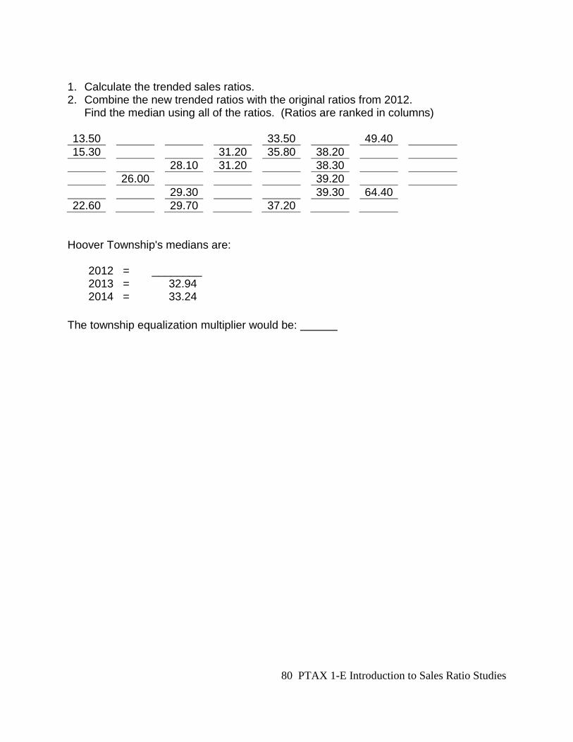
80 PTAX 1-E Introduction to Sales Ratio Studies
1. Calculate the trended sales ratios. 2. Combine the new trended ratios with the original ratios from 2012.
Find the median using all of the ratios. (Ratios are ranked in columns) 13.50 33.50 49.40
15.30 31.20 35.80 38.20
28.10 31.20 38.30
26.00 39.20
29.30 39.30 64.40
22.60 29.70 37.20
Hoover Township's medians are: 2012 = ________ 2013 = 32.94 2014 = 33.24
The township equalization multiplier would be:
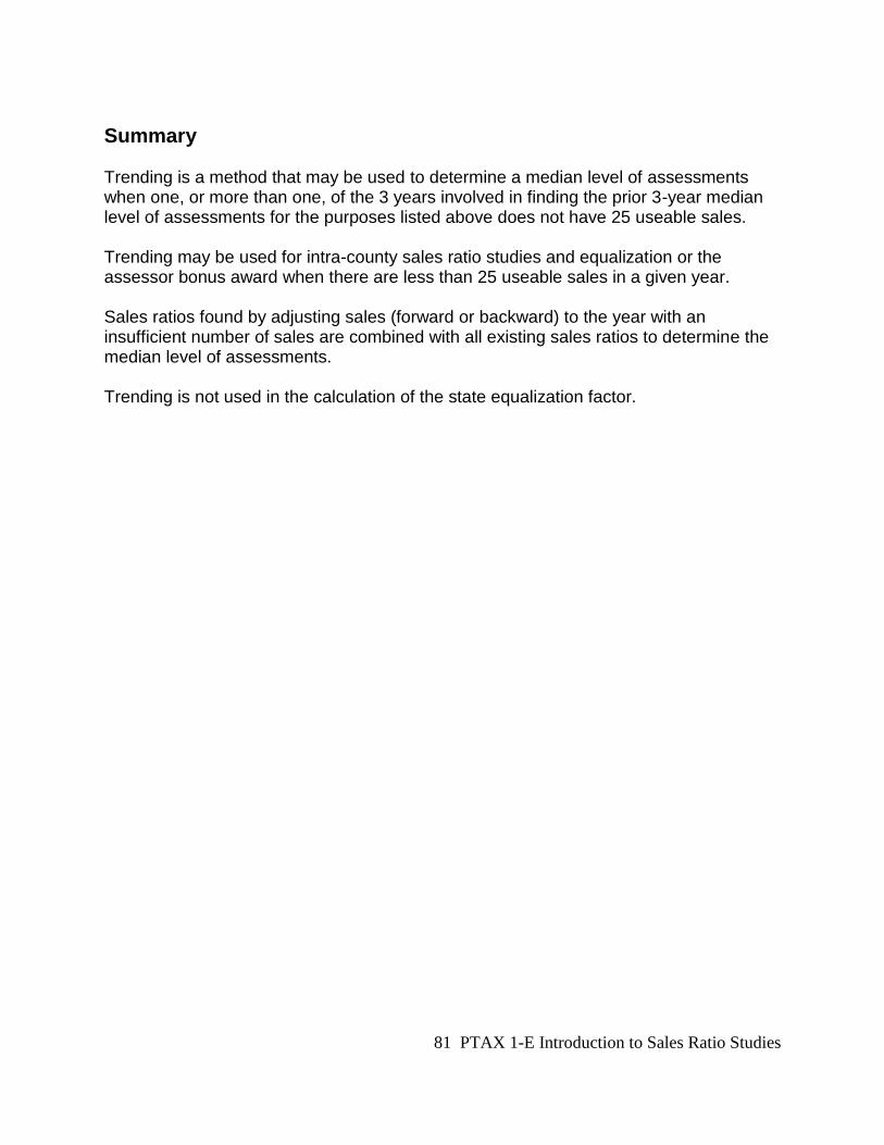
81 PTAX 1-E Introduction to Sales Ratio Studies
Summary Trending is a method that may be used to determine a median level of assessments when one, or more than one, of the 3 years involved in finding the prior 3-year median level of assessments for the purposes listed above does not have 25 useable sales. Trending may be used for intra-county sales ratio studies and equalization or the assessor bonus award when there are less than 25 useable sales in a given year. Sales ratios found by adjusting sales (forward or backward) to the year with an insufficient number of sales are combined with all existing sales ratios to determine the median level of assessments. Trending is not used in the calculation of the state equalization factor.
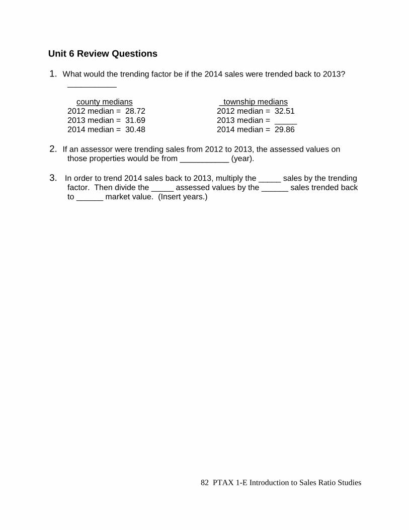
82 PTAX 1-E Introduction to Sales Ratio Studies
Unit 6 Review Questions
1. What would the trending factor be if the 2014 sales were trended back to 2013? ___________ county medians township medians 2012 median = 28.72 2012 median = 32.51 2013 median = 31.69 2013 median = _____ 2014 median = 30.48 2014 median = 29.86
2. If an assessor were trending sales from 2012 to 2013, the assessed values on those properties would be from ___________ (year).
3. In order to trend 2014 sales back to 2013, multiply the _____ sales by the trending factor. Then divide the _____ assessed values by the ______ sales trended back to ______ market value. (Insert years.)
83 PTAX 1-E Introduction to Sales Ratio Studies
Unit 7 The Sales Ratio Study: Table 1 This unit covers Table 1 from the Sales Ratio Study. The “I-E Class Sales Ratio Study” is found in the Supplemental section at the back of the packet. This unit focuses on the understanding and interpretation of the sales ratio studies. The purpose of this unit is to familiarize township assessors and supervisors of assessments with the sales ratio study and the information that can be gathered from it. Particular emphasis is on the median level of assessments, measures of assessment uniformity, and equalization. The “I-E Class Sales Ratio Study” has fictitious counties and townships. Its purpose is to become familiar with the information and format of the sales ratio study. Learning Objectives: After completing the assigned readings, you should be able to:
find the median level of assessments for a county or township
locate the measures of assessment uniformity for a jurisdiction
determine whether a jurisdiction is assessing uniformly
analyze what types of properties are most in need of reassessment
84 PTAX 1-E Introduction to Sales Ratio Studies
Table 1: Assessment Ratios Turn to the I-E Class Sales Ratio Study in the supplemental section at the back of the manual. 1 Columns in Table 1 of the sales ratio study: 1. Geographic Area: name of the county or township.
2. Urban when all of the useable sales are included; “Unimp” is only displayed when there are 25 or more useable sales for the category, otherwise urban indicates improved sales only.
3. Adjusted Median found by adjusting the calculated median for changes due to reassessment. The adjusted median is the median used in the calculation of the equalization factors.
4. Median as calculated from the sales ratio study.
5. COD
6. Sales: number of sales used in the sales ratio study.
7. 1st Quartile: ratio such that 25% (¼) of the ratios are smaller than the number listed and 75% (¾) of the ratios are larger than the ratio listed.
8. 3rd Quartile: ratio such that 75% (¾) of the ratios are smaller than the number listed and 25% (¼) of the ratios are larger than the ratio listed.
9. Ratio Range: the difference between the largest sales ratio and the smallest sales ratio.
10. PRD
11. 95% Confidence Interval: the ratio range such that there is a 95% assurance that the true median of all properties falls within this range.
12. COC Begin by looking at the first county on the list: Arthur County. All of the townships have “Urban” in the second column. “Urban” refers to studies that exclude farm sales. Now look at “Baker County.” Apple River township has “Urban” directly to the right of the township name. “Urban” refers to the total number of useable non-farm sales in the county or township. Below “Urban” is “Imp” which stands for improved properties and “Unimp” which stands for unimproved properties. For all counties other than Cook, the Department calculates median assessment levels for both “improved” and “unimproved” urban property when there are 25 or more useable sales in each of these subcategories. This information helps local assessing officials identify the presence or absence of a systematic bias toward higher or lower assessment levels on unimproved property. Look at the 6th column whose
1 This table is for illustrative purposes only. The table is similar in form to the actual Table 1 Assessment Ratios published by the Department of Revenue.
85 PTAX 1-E Introduction to Sales Ratio Studies
heading is “Sales.” For Apple River township there were a total of 141 useable sales. Of these 31 were improved properties and 110 were unimproved. The heading for the fourth column is “Median.” This is the median as calculated from the sales ratio study before any adjustments are made. For the sales ratio study, found on Page 25, the median was calculated to be 32.50%. For Ferrari township in Autobahn county, the median as calculated is 28.62%. The heading of the third column is “Adjusted Median.” This is the calculated median from the fourth column after adjustments for changes due to reassessment or equalization by the CCAO or the board of review. In Duke county, Water Well township has a (raw) median of 32.41%. Notice that the adjusted median for Water Well township has a “–“ in the adjusted median column. This indicates that the adjusted median is the same as the (raw) median of 32.41%. There are 11 counties in this classroom sales ratio study. Looking at the “Total County” row and the “Median” column, find the county whose median is closest to 33.33%. ______________ Find the county with the median of 29.57% ________________.
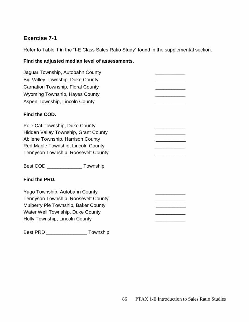
86 PTAX 1-E Introduction to Sales Ratio Studies
Exercise 7-1 Refer to Table 1 in the “I-E Class Sales Ratio Study” found in the supplemental section. Find the adjusted median level of assessments. Jaguar Township, Autobahn County ___________
Big Valley Township, Duke County ___________
Carnation Township, Floral County ___________
Wyoming Township, Hayes County ___________
Aspen Township, Lincoln County ___________
Find the COD. Pole Cat Township, Duke County ___________
Hidden Valley Township, Grant County ___________
Abilene Township, Harrison County ___________
Red Maple Township, Lincoln County ___________
Tennyson Township, Roosevelt County ___________
Best COD _____________ Township
Find the PRD.
Yugo Township, Autobahn County ___________
Tennyson Township, Roosevelt County ___________
Mulberry Pie Township, Baker County ___________
Water Well Township, Duke County ___________
Holly Township, Lincoln County ___________
Best PRD _______________ Township
87 PTAX 1-E Introduction to Sales Ratio Studies
Find the COC. Lamborghini Township, Autobahn County ___________
Abilene Township, Harrison County ___________
Peach Cobbler Township, Baker County ___________
Daisy Township, Duke County ___________
Walnut Grove Township, Lincoln County ___________
Best COC ________________ Township
Assessment Ratios for Lincoln County
The Supervisor of Assessments wants to determine whether there is a difference in uniformity between improved and unimproved properties. Several townships have enough sales to have sales ratio studies done by these sub-categories. He or she decides to look at all of the available measures of uniformity listed in the sales ratio study book. By comparing the unimproved properties to the improved properties for the townships that had enough sales to conduct sales ratio studies for the sub-categories of “Improved” and “Unimproved”, determine which type of property was most uniformly assessed for each of the measures of uniformity listed.
a. For the COD:
Improved Unimproved
Blue Spruce ___________ __________
Cherry ___________ __________
Cottonwood ___________ __________
Hawthorn ___________ __________
Most uniform (COD) is (unimproved, improved) ____________
b. For the COC:
Improved Unimproved
Blue Spruce ___________ __________
Cherry ___________ __________
Cottonwood ___________ __________
Hawthorn ___________ __________
Most uniform (COC) is (unimproved, improved) _____________
88 PTAX 1-E Introduction to Sales Ratio Studies
c. For the PRD: Improved Unimproved
Blue Spruce ___________ __________
Cherry ___________ __________
Cottonwood ___________ __________
Hawthorn ___________ __________
Most uniform (PRD) is (unimproved, improved) _____________
Overall, which type of property should she concentrate on for reassessment?
__________________
89 PTAX 1-E Introduction to Sales Ratio Studies
Summary The sales ratio study as performed by the Department of Revenue provides multiple tools for a more complete grasp of assessment uniformity within the county. The sales ratio study, as it appears in “Table 1 Assessment Ratios”, provides the assessor with information necessary to determine what townships would be most helped by reassessment. The assessor, using the calculations of the median, the COD, the PRD, and the COC, may make a better determination on how to most effectively utilize limited time and resources to improve assessment uniformity.
90 PTAX 1-E Introduction to Sales Ratio Studies
Unit 7 Review Questions Assessment Ratios for FLORAL COUNTY Refer to the “I-E Class Sales Ratio Study” in the supplemental section.
1. What was the median assessment ratio for Carnation township? __________
2. Begonia township was under-assessed, statutorily assessed, or over-assessed? __________
3. Which township was assessing closest to the statutory level (use adjusted median)? __________
4. Considering only the COD, name the township that was: least uniformly assessed. ___________________________ most uniformly assessed. ___________________________
91 PTAX 1-E Introduction to Sales Ratio Studies
Homework Answers follow the page the exercise is presented on.
Interquartile Range Calculations Calculate the upper and lower trim limits for the following group of numbers: 7.81, 17.46, 17.89, 20.00, 35.23, 38.99, 40.77, 50.22, 51.33, 51.87, 59.82, 62.37, 65.79, 89.99, 125.66 1. First Quartile: ____ 2. Third Quartile: ____ 3. Interquartile range: _______ 4. Interquartile range ___ x 6 = ______ 5. Third Quartile + Result = ______ 6. First Quartile – Result = ______ Are there any numbers removed from this group? ___
92 PTAX 1-E Introduction to Sales Ratio Studies
1. First Quartile: 4 2. Third Quartile: 12 3. Interquartile range: 42.37 4. Interquartile range 42.37 x 6 = 254.22 5. Third Quartile + Result = 316.59 6. First Quartile – Result = -234.22 Are there any numbers removed from this group? No
93 PTAX 1-E Introduction to Sales Ratio Studies
TOWNSHIP #2
Sales Av Sale Price Ratio (%) Ranked Deviation
$ 22,097 $ 124,000 _________ ________ _________
36,098 117,500 _________ ________ _________
37,474 98,000 _________ ________ _________
31,520 105,000 _________ ________ _________
28,064 62,900 _________ ________ _________
10,475 24,600 _________ ________ _________
24,522 79,000 _________ ________ _________
37,475 138,700 _________ ________ _________
35,176 85,000 _________ ________ _________
18,931 72,400 _________ ________ _________
22,258 58,200 _________ ________ _________
5,210 12,800 _________ ________ _________
28,285 87,300 _________ ________ _________
31,845 113,000 _________ ________ _________
27,407 82,900 _________ ________ _________
7,319 18,700 _________ ________ _________
20,744 69,500 _________ ________ _________
31,548 92,300 _________ ________ _________
_________ _______ _________ __________
Median Level of Assessment ____________
Coefficient of Dispersion (COD) ____________
Coefficient of Concentration (COC) ____________
Price Related Differential (PRD) ____________
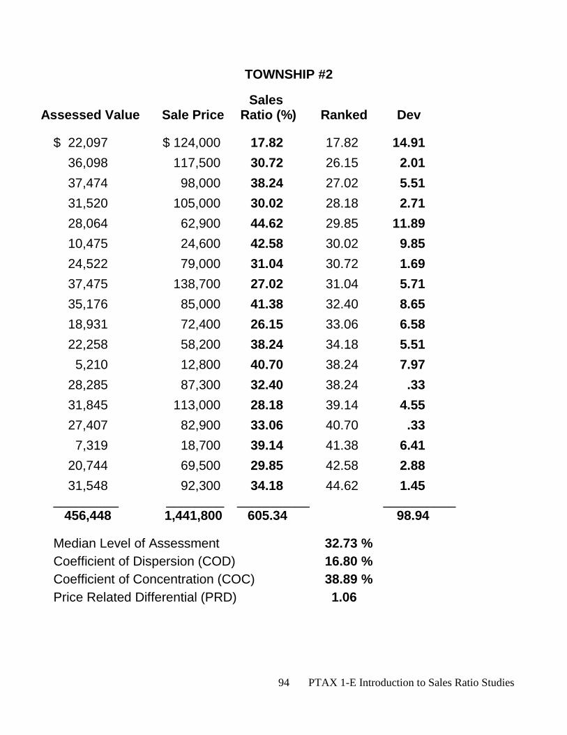
94 PTAX 1-E Introduction to Sales Ratio Studies
TOWNSHIP #2
Sales Assessed Value Sale Price Ratio (%) Ranked Dev
$ 22,097 $ 124,000 17.82 17.82 14.91
36,098 117,500 30.72 26.15 2.01
37,474 98,000 38.24 27.02 5.51
31,520 105,000 30.02 28.18 2.71
28,064 62,900 44.62 29.85 11.89
10,475 24,600 42.58 30.02 9.85
24,522 79,000 31.04 30.72 1.69
37,475 138,700 27.02 31.04 5.71
35,176 85,000 41.38 32.40 8.65
18,931 72,400 26.15 33.06 6.58
22,258 58,200 38.24 34.18 5.51
5,210 12,800 40.70 38.24 7.97
28,285 87,300 32.40 38.24 .33
31,845 113,000 28.18 39.14 4.55
27,407 82,900 33.06 40.70 .33
7,319 18,700 39.14 41.38 6.41
20,744 69,500 29.85 42.58 2.88
31,548 92,300 34.18 44.62 1.45 _________ ________ __________ __________ 456,448 1,441,800 605.34 98.94
Median Level of Assessment 32.73 %
Coefficient of Dispersion (COD) 16.80 %
Coefficient of Concentration (COC) 38.89 %
Price Related Differential (PRD) 1.06
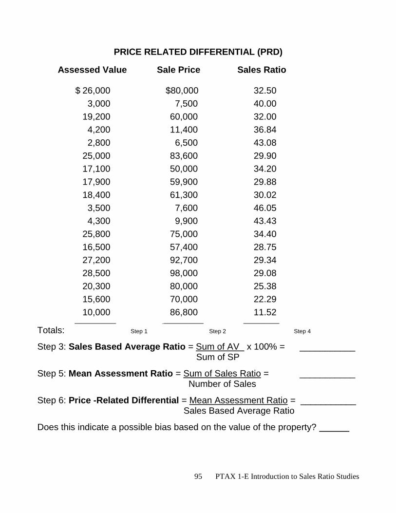
95 PTAX 1-E Introduction to Sales Ratio Studies
PRICE RELATED DIFFERENTIAL (PRD)
Assessed Value Sale Price Sales Ratio $ 26,000 $80,000 32.50
3,000 7,500 40.00
19,200 60,000 32.00
4,200 11,400 36.84
2,800 6,500 43.08
25,000 83,600 29.90
17,100 50,000 34.20
17,900 59,900 29.88
18,400 61,300 30.02
3,500 7,600 46.05
4,300 9,900 43.43
25,800 75,000 34.40
16,500 57,400 28.75
27,200 92,700 29.34
28,500 98,000 29.08
20,300 80,000 25.38
15,600 70,000 22.29
10,000 86,800 11.52 _______________________ _______________________ ____________________
Totals: Step 1 Step 2 Step 4
Step 3: Sales Based Average Ratio = Sum of AV x 100% = ___________ Sum of SP
Step 5: Mean Assessment Ratio = Sum of Sales Ratio = ___________ Number of Sales
Step 6: Price -Related Differential = Mean Assessment Ratio = ___________ Sales Based Average Ratio
Does this indicate a possible bias based on the value of the property?
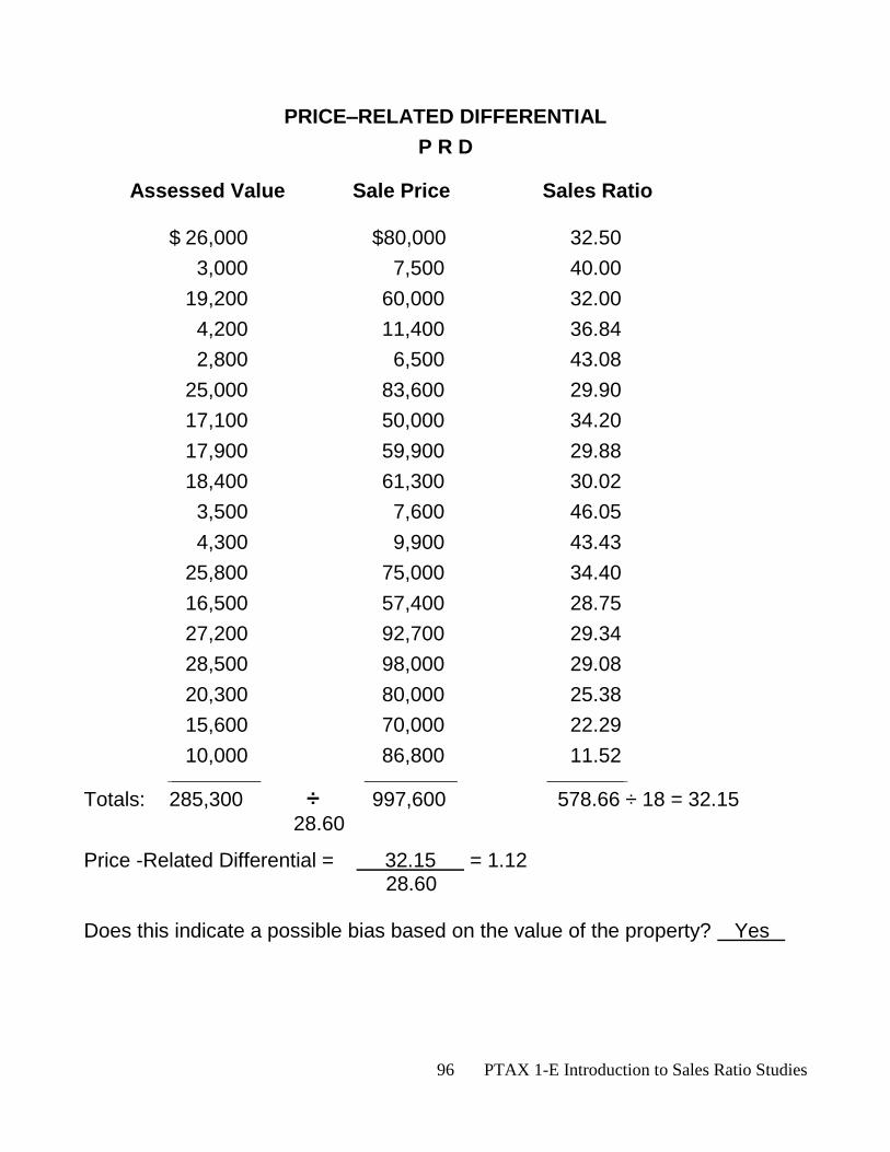
96 PTAX 1-E Introduction to Sales Ratio Studies
PRICE–RELATED DIFFERENTIAL
P R D
Assessed Value Sale Price Sales Ratio $ 26,000 $80,000 32.50
3,000 7,500 40.00
19,200 60,000 32.00
4,200 11,400 36.84
2,800 6,500 43.08
25,000 83,600 29.90
17,100 50,000 34.20
17,900 59,900 29.88
18,400 61,300 30.02
3,500 7,600 46.05
4,300 9,900 43.43
25,800 75,000 34.40
16,500 57,400 28.75
27,200 92,700 29.34
28,500 98,000 29.08
20,300 80,000 25.38
15,600 70,000 22.29
10,000 86,800 11.52 _______________________ _______________________ ____________________
Totals: 285,300 ÷ 997,600 578.66 ÷ 18 = 32.15
28.60
Price -Related Differential = 32.15 = 1.12 28.60 Does this indicate a possible bias based on the value of the property? Yes
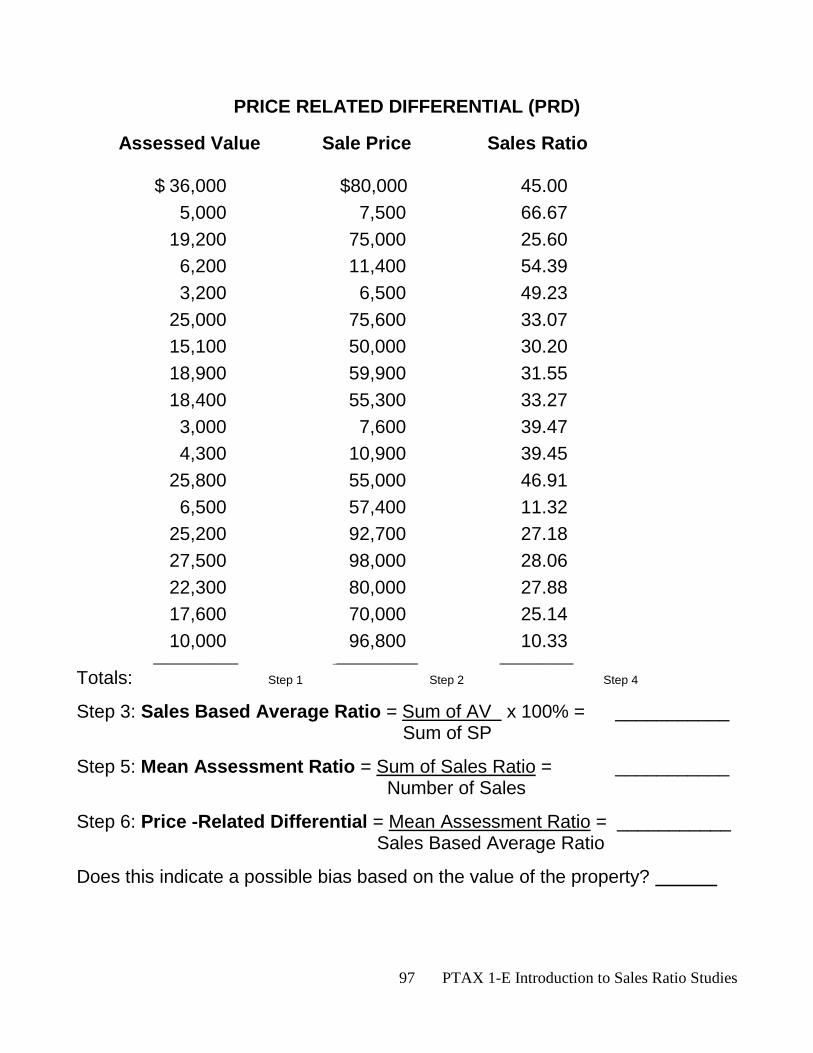
97 PTAX 1-E Introduction to Sales Ratio Studies
PRICE RELATED DIFFERENTIAL (PRD)
Assessed Value Sale Price Sales Ratio $ 36,000 $80,000 45.00
5,000 7,500 66.67
19,200 75,000 25.60
6,200 11,400 54.39
3,200 6,500 49.23
25,000 75,600 33.07
15,100 50,000 30.20
18,900 59,900 31.55
18,400 55,300 33.27
3,000 7,600 39.47
4,300 10,900 39.45
25,800 55,000 46.91
6,500 57,400 11.32
25,200 92,700 27.18
27,500 98,000 28.06
22,300 80,000 27.88
17,600 70,000 25.14
10,000 96,800 10.33 _______________________ _______________________ ____________________
Totals: Step 1 Step 2 Step 4
Step 3: Sales Based Average Ratio = Sum of AV x 100% = ___________ Sum of SP
Step 5: Mean Assessment Ratio = Sum of Sales Ratio = ___________ Number of Sales
Step 6: Price -Related Differential = Mean Assessment Ratio = ___________ Sales Based Average Ratio
Does this indicate a possible bias based on the value of the property?
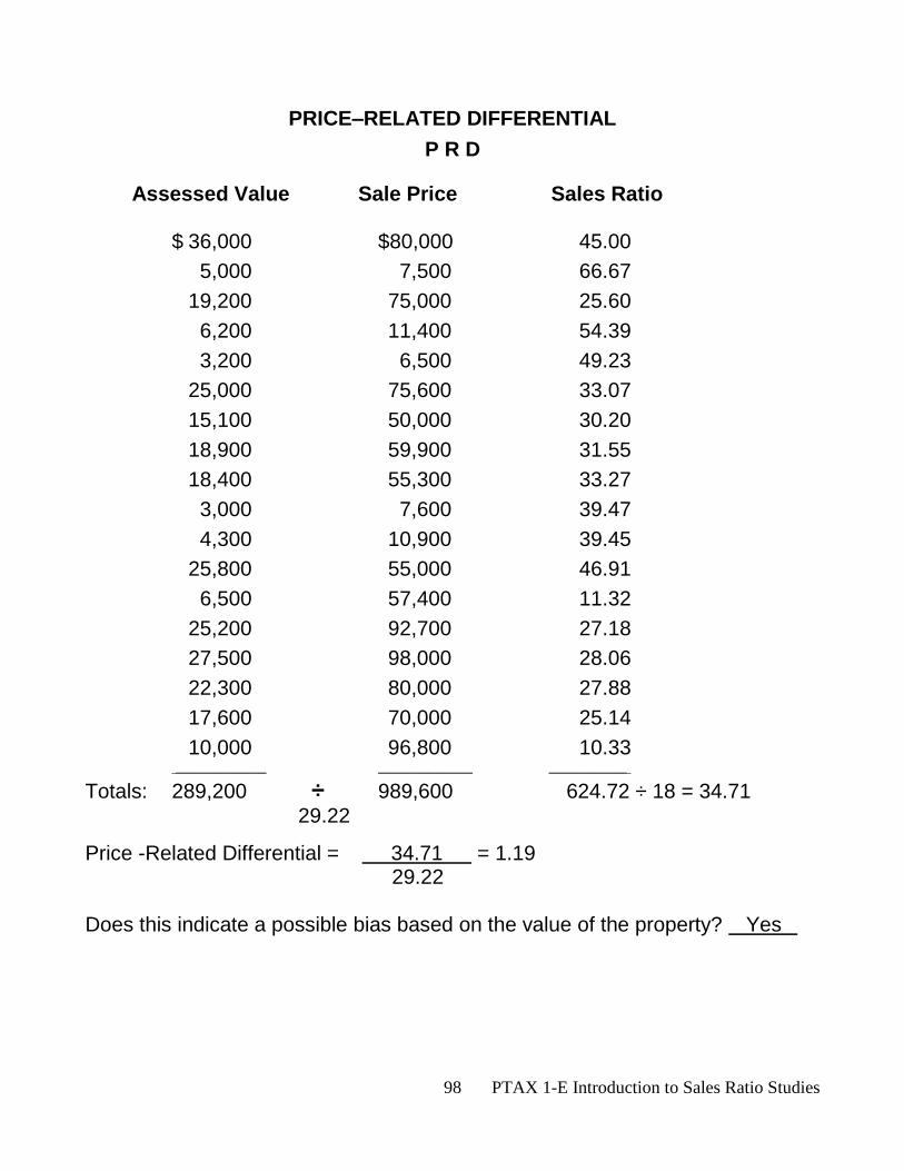
98 PTAX 1-E Introduction to Sales Ratio Studies
PRICE–RELATED DIFFERENTIAL
P R D
Assessed Value Sale Price Sales Ratio $ 36,000 $80,000 45.00
5,000 7,500 66.67
19,200 75,000 25.60
6,200 11,400 54.39
3,200 6,500 49.23
25,000 75,600 33.07
15,100 50,000 30.20
18,900 59,900 31.55
18,400 55,300 33.27
3,000 7,600 39.47
4,300 10,900 39.45
25,800 55,000 46.91
6,500 57,400 11.32
25,200 92,700 27.18
27,500 98,000 28.06
22,300 80,000 27.88
17,600 70,000 25.14
10,000 96,800 10.33 _______________________ _______________________ ____________________
Totals: 289,200 ÷ 989,600 624.72 ÷ 18 = 34.71
29.22
Price -Related Differential = 34.71 = 1.19 29.22 Does this indicate a possible bias based on the value of the property? Yes
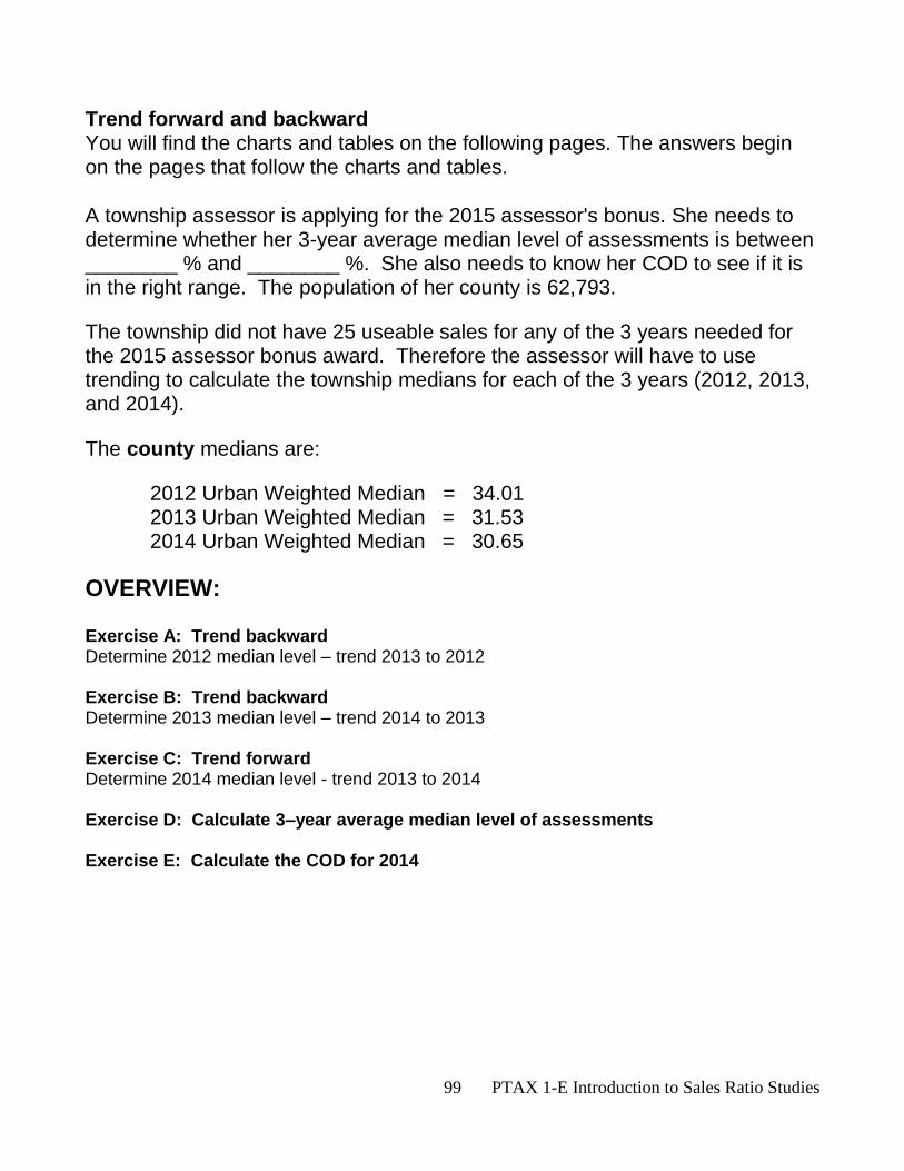
99 PTAX 1-E Introduction to Sales Ratio Studies
Trend forward and backward You will find the charts and tables on the following pages. The answers begin on the pages that follow the charts and tables.
A township assessor is applying for the 2015 assessor's bonus. She needs to determine whether her 3-year average median level of assessments is between ________ % and ________ %. She also needs to know her COD to see if it is in the right range. The population of her county is 62,793.
The township did not have 25 useable sales for any of the 3 years needed for the 2015 assessor bonus award. Therefore the assessor will have to use trending to calculate the township medians for each of the 3 years (2012, 2013, and 2014).
The county medians are:
2012 Urban Weighted Median = 34.01 2013 Urban Weighted Median = 31.53 2014 Urban Weighted Median = 30.65
OVERVIEW: Exercise A: Trend backward Determine 2012 median level – trend 2013 to 2012 Exercise B: Trend backward Determine 2013 median level – trend 2014 to 2013 Exercise C: Trend forward Determine 2014 median level - trend 2013 to 2014 Exercise D: Calculate 3–year average median level of assessments Exercise E: Calculate the COD for 2014
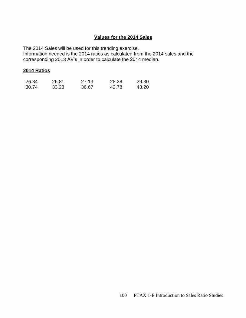
100 PTAX 1-E Introduction to Sales Ratio Studies
Values for the 2014 Sales
The 2014 Sales will be used for this trending exercise. Information needed is the 2014 ratios as calculated from the 2014 sales and the corresponding 2013 AV’s in order to calculate the 2014 median. 2014 Ratios 26.34 26.81 27.13 28.38 29.30 30.74 33.23 36.67 42.78 43.20
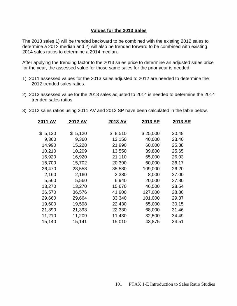
101 PTAX 1-E Introduction to Sales Ratio Studies
Values for the 2013 Sales
The 2013 sales 1) will be trended backward to be combined with the existing 2012 sales to determine a 2012 median and 2) will also be trended forward to be combined with existing 2014 sales ratios to determine a 2014 median. After applying the trending factor to the 2013 sales price to determine an adjusted sales price for the year, the assessed value for those same sales for the prior year is needed. 1) 2011 assessed values for the 2013 sales adjusted to 2012 are needed to determine the
2012 trended sales ratios.
2) 2013 assessed value for the 2013 sales adjusted to 2014 is needed to determine the 2014 trended sales ratios.
3) 2012 sales ratios using 2011 AV and 2012 SP have been calculated in the table below.
2011 AV 2012 AV 2013 AV 2013 SP 2013 SR
$ 5,120 $ 5,120 $ 8,510 $ 25,000 20.48
9,360 9,360 13,150 40,000 23.40
14,990 15,228 21,990 60,000 25.38
10,210 10,209 13,550 39,800 25.65
16,920 16,920 21,110 65,000 26.03
15,700 15,702 20,390 60,000 26.17
26,470 28,558 35,580 109,000 26.20
2,160 2,160 2,380 8,000 27.00
5,560 5,560 6,940 20,000 27.80
13,270 13,270 15,670 46,500 28.54
36,570 36,576 41,900 127,000 28.80
29,660 29,664 33,340 101,000 29.37
19,600 19,598 22,430 65,000 30.15
21,390 21,393 22,330 68,000 31.46
11,210 11,209 11,430 32,500 34.49
15,140 15,141 15,010 43,875 34.51
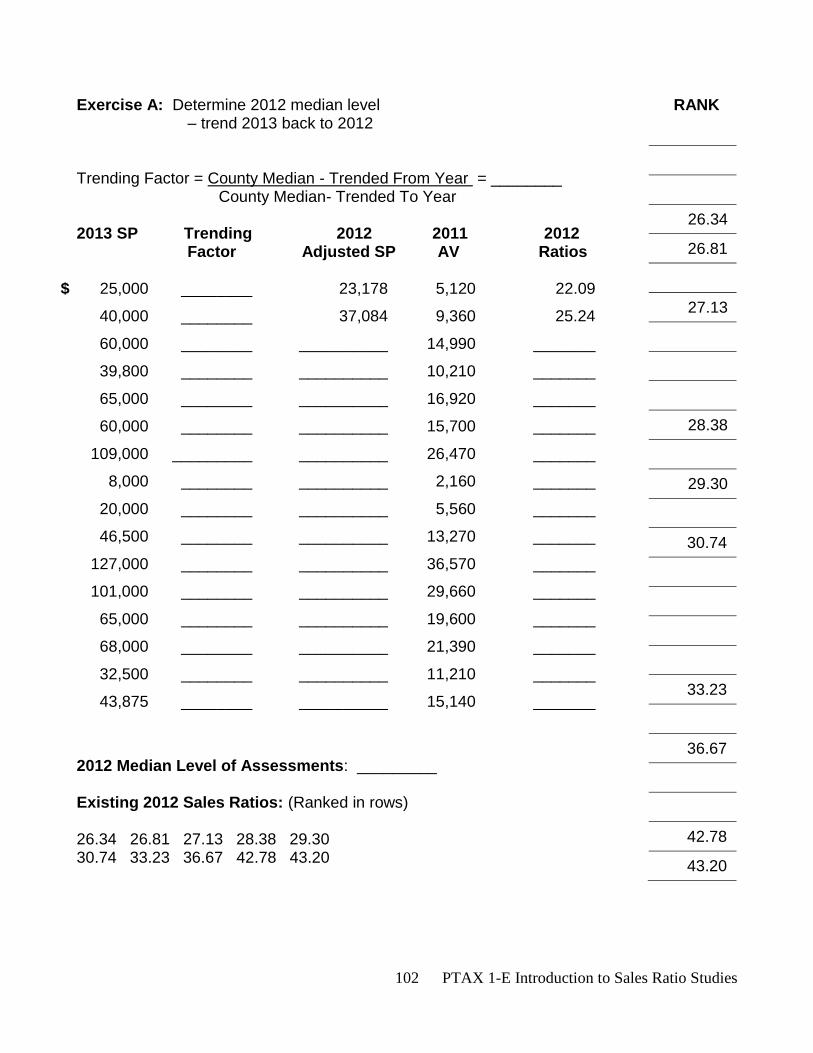
102 PTAX 1-E Introduction to Sales Ratio Studies
Exercise A: Determine 2012 median level RANK – trend 2013 back to 2012 Trending Factor = County Median - Trended From Year = ________ County Median- Trended To Year 2013 SP Trending 2012 2011 2012 Factor Adjusted SP AV Ratios
$ 25,000 ________ 23,178 5,120 22.09
40,000 ________ 37,084 9,360 25.24
60,000 ________ __________ 14,990 _______
39,800 ________ __________ 10,210 _______
65,000 ________ __________ 16,920 _______
60,000 ________ __________ 15,700 _______
109,000 _________ __________ 26,470 _______
8,000 ________ __________ 2,160 _______
20,000 ________ __________ 5,560 _______
46,500 ________ __________ 13,270 _______
127,000 ________ __________ 36,570 _______
101,000 ________ __________ 29,660 _______
65,000 ________ __________ 19,600 _______
68,000 ________ __________ 21,390 _______
32,500 ________ __________ 11,210 _______
43,875 ________ __________ 15,140 _______
2012 Median Level of Assessments: _________ Existing 2012 Sales Ratios: (Ranked in rows) 26.34 26.81 27.13 28.38 29.30 30.74 33.23 36.67 42.78 43.20
26.34
26.81
27.13
28.38
29.30
30.74
33.23
36.67
42.78
43.20
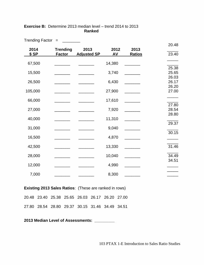
103 PTAX 1-E Introduction to Sales Ratio Studies
Exercise B: Determine 2013 median level – trend 2014 to 2013 Ranked
Trending Factor = ________ 20.48 2014 Trending 2013 2012 2013 _____ $ SP Factor Adjusted SP AV Ratios 23.40 _____ 67,500 _______ _______ 14,380 _______ _____ 25.38 15,500 _______ _______ 3,740 _______ 25.65 26.03 26,500 _______ _______ 6,430 _______ 26.17 26.20 105,000 _______ _______ 27,900 _______ 27.00 _____ 66,000 _______ _______ 17,610 _______ _____ 27.80 27,000 _______ _______ 7,920 _______ 28.54 28.80 40,000 _______ _______ 11,310 _______ _____ 29.37 31,000 _______ _______ 9,040 _______ _____ 30.15 16,500 _______ _______ 4,870 _______ _____ _____ 42,500 _______ _______ 13,330 _______ 31.46 _____ 28,000 _______ _______ 10,040 _______ 34.49 34.51 12,000 _______ _______ 4,990 _______ _____ _____ 7,000 _______ _______ 8,300 _______ _____ Existing 2013 Sales Ratios: (These are ranked in rows) 20.48 23.40 25.38 25.65 26.03 26.17 26.20 27.00 27.80 28.54 28.80 29.37 30.15 31.46 34.49 34.51 2013 Median Level of Assessments: _________
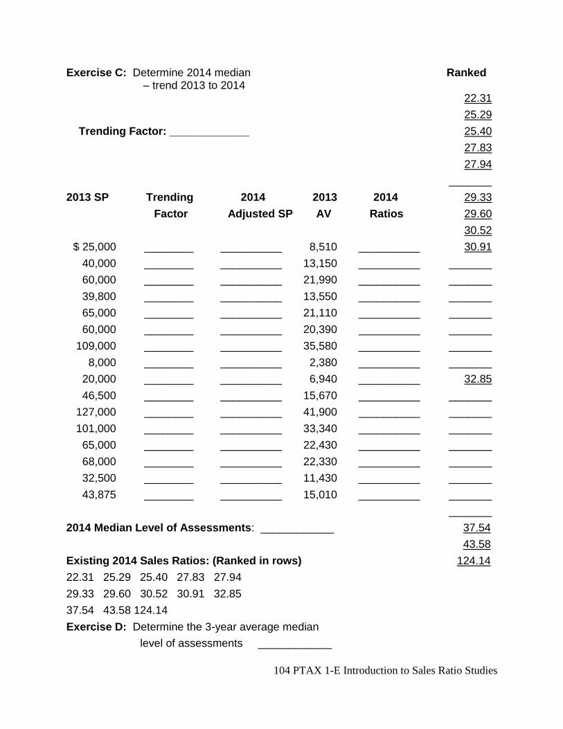
104 PTAX 1-E Introduction to Sales Ratio Studies
Exercise C: Determine 2014 median Ranked – trend 2013 to 2014 22.31
25.29
Trending Factor: _____________ 25.40
27.83
27.94
_______
2013 SP Trending 2014 2013 2014 29.33
Factor Adjusted SP AV Ratios 29.60
30.52
$ 25,000 ________ __________ 8,510 __________ 30.91
40,000 ________ __________ 13,150 __________ _______
60,000 ________ __________ 21,990 __________ _______
39,800 ________ __________ 13,550 __________ _______
65,000 ________ __________ 21,110 __________ _______
60,000 ________ __________ 20,390 __________ _______
109,000 ________ __________ 35,580 __________ _______
8,000 ________ __________ 2,380 __________ _______
20,000 ________ __________ 6,940 __________ 32.85
46,500 ________ __________ 15,670 __________ _______
127,000 ________ __________ 41,900 __________ _______
101,000 ________ __________ 33,340 __________ _______
65,000 ________ __________ 22,430 __________ _______
68,000 ________ __________ 22,330 __________ _______
32,500 ________ __________ 11,430 __________ _______
43,875 ________ __________ 15,010 __________ _______
_______
2014 Median Level of Assessments: ____________ 37.54
43.58
Existing 2014 Sales Ratios: (Ranked in rows) 124.14
22.31 25.29 25.40 27.83 27.94
29.33 29.60 30.52 30.91 32.85
37.54 43.58 124.14
Exercise D: Determine the 3-year average median
level of assessments ____________
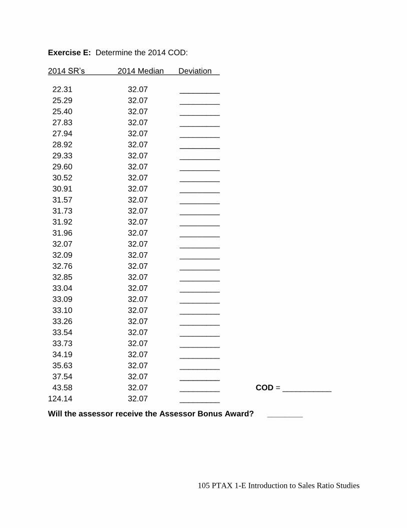
105 PTAX 1-E Introduction to Sales Ratio Studies
Exercise E: Determine the 2014 COD: 2014 SR’s 2014 Median Deviation 22.31 32.07 _________
25.29 32.07 _________
25.40 32.07 _________
27.83 32.07 _________
27.94 32.07 _________
28.92 32.07 _________
29.33 32.07 _________
29.60 32.07 _________
30.52 32.07 _________
30.91 32.07 _________
31.57 32.07 _________
31.73 32.07 _________
31.92 32.07 _________
31.96 32.07 _________
32.07 32.07 _________
32.09 32.07 _________
32.76 32.07 _________
32.85 32.07 _________
33.04 32.07 _________
33.09 32.07 _________
33.10 32.07 _________
33.26 32.07 _________
33.54 32.07 _________
33.73 32.07 _________
34.19 32.07 _________
35.63 32.07 _________
37.54 32.07 _________
43.58 32.07 _________ COD = ___________
124.14 32.07 _________
Will the assessor receive the Assessor Bonus Award? ________
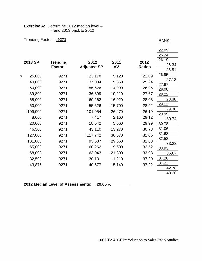
106 PTAX 1-E Introduction to Sales Ratio Studies
Exercise A: Determine 2012 median level – trend 2013 back to 2012 Trending Factor = .9271 2013 SP Trending 2012 2011 2012 Factor Adjusted SP AV Ratios
$ 25,000 .9271 23,178 5,120 22.09
40,000 .9271 37,084 9,360 25.24
60,000 .9271 55,626 14,990 26.95
39,800 .9271 36,899 10,210 27.67
65,000 .9271 60,262 16,920 28.08
60,000 .9271 55,626 15,700 28.22
109,000 .9271 101,054 26,470 26.19
8,000 .9271 7,417 2,160 29.12
20,000 .9271 18,542 5,560 29.99
46,500 .9271 43,110 13,270 30.78
127,000 .9271 117,742 36,570 31.06
101,000 .9271 93,637 29,660 31.68
65,000 .9271 60,262 19,600 32.52
68,000 .9271 63,043 21,390 33.93
32,500 .9271 30,131 11,210 37.20
43,875 .9271 40,677 15,140 37.22
2012 Median Level of Assessments: 29.65 %
RANK
22.09
25.24
26.19
26.34
26.81
26.95
27.13
27.67
28.08
28.22
28.38
29.12
29.30
29.99
30.74
30.78
31.06
31.68
32.52
33.23
33.93
36.67
37.20
37.22
42.78
43.20
107 PTAX 1-E Introduction to Sales Ratio Studies
Exercise B: Determine 2013 median level – trend 2014 to 2013 Trending Factor = .9721 20.48 2014 Trending 2013 2012 2013 21.92 $ SP Factor Adjusted SP AV Ratios 23.40 24.82 67,500 .9721 65,617 14,380 21.92 24.96 25.38 15,500 .9721 15,068 3,740 24.82 25.65 26.03 26,500 .9721 25,761 6,430 24.96 26.17 26.20 105,000 .9721 102,071 27,900 27.33 27.00 27.33 66,000 .9721 64,159 17,610 27.45 27.45 27.80 27,000 .9721 26,247 7,920 30.17 28.54 28.80 40,000 .9721 38,884 11,310 29.09 29.09 29.37 31,000 .9721 30,135 9,040 30.00 30.00 30.15 16,500 .9721 16,040 4,870 30.36 30.17 30.36 42,500 .9721 41,314 13,330 32.27 31.46 32.27 28,000 .9721 27,219 10,040 36.89 34.49 34.51 12,000 .9721 11,665 4,990 42.78 36.89 42.78 7,000 .9721 6,805 8,300 121.97 121.97 2013 Median Level of Assessments: 28.54 %
108 PTAX 1-E Introduction to Sales Ratio Studies
Exercise C: Determine 2014 median level Ranked Trend 2013 to 2014 22.31
25.29
Trending Factor 1.0287 25.40
27.83
27.94
28.92
2013 SP Trending 2014 2013 2014 29.33
Factor Adjusted SP AV Ratios 29.60
30.52
$ 25,000 1.0287 25,718 8,510 33.09 30.91
40,000 1.0287 41,148 13,150 31.96 31.57
60,000 1.0287 61,722 21,990 35.63 31.73
39,800 1.0287 40,942 13,550 33.10 31.92
65,000 1.0287 66,866 21,110 31.57 31.96
60,000 1.0287 61,722 20,390 33.04 32.07
109,000 1.0287 112,128 35,580 31.73 32.09
8,000 1.0287 8,230 2,380 28.92 32.76
20,000 1.0287 20,574 6,940 33.73 32.85
46,500 1.0287 47,835 15,670 32.76 33.04
127,000 1.0287 130,645 41,900 32.07 33.09
101,000 1.0287 103,899 33,340 32.09 33.10
65,000 1.0287 66,866 22,430 33.54 33.26
68,000 1.0287 69,952 22,330 31.92 33.54
32,500 1.0287 33,433 11,430 34.19 33.73
43,875 1.0287 45,134 15,010 33.26 34.19
35.63
2013 Median Level of Assessments: 32.07 % 37.54
43.58 Exercise D: Determine the 3-year average median 124.14
level of assessments 30.09 %
109 PTAX 1-E Introduction to Sales Ratio Studies
Exercise E: Determine the 2014 COD:
2014 SR’s 2014 Median Deviation 22.31 32.07 9.76
25.29 32.07 6.78
25.40 32.07 6.67
27.83 32.07 4.24
27.94 32.07 4.13
28.92 32.07 3.15
29.33 32.07 2.74
29.60 32.07 2.47
30.52 32.07 1.55
30.91 32.07 1.16
31.57 32.07 .50
31.73 32.07 .34
31.92 32.07 .15
31.96 32.07 .11
32.07 32.07 .00
32.09 32.07 .02
32.76 32.07 .69
32.85 32.07 .78
33.04 32.07 .97
33.09 32.07 1.02
33.10 32.07 1.03
33.26 32.07 1.19
33.54 32.07 1.47
33.73 32.07 1.66
34.19 32.07 2.12
35.63 32.07 3.56
37.54 32.07 5.47
43.58 32.07 11.51 COD = 17.99%
124.14 32.07 92.07
Total 167.20
Will the assessor receive the Assessor Bonus Award? NO
110 PTAX 1-E Introduction to Sales Ratio Studies
Find the COD for this township TOWNSHIP Prior Year Current Year Sales Ratio AV Sale Price % $ 15,700 $ 57,900 27.12
35,600 98,300 36.22
24,800 72,900 34.02
16,300 56,100 29.06
19,500 68,400 28.51
32,100 83,100 38.63
14,000 47,500 29.47
35,600 93,800 37.95
COD = _________
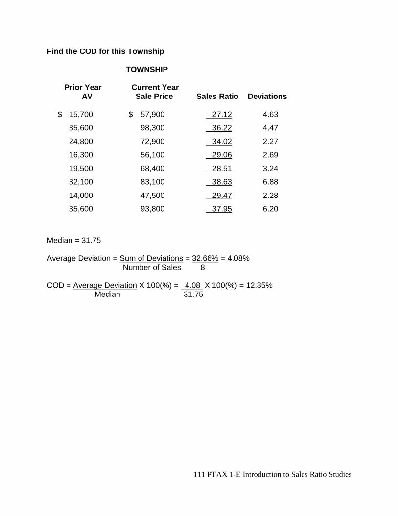
111 PTAX 1-E Introduction to Sales Ratio Studies
Find the COD for this Township TOWNSHIP Prior Year Current Year AV Sale Price Sales Ratio Deviations $ 15,700 $ 57,900 27.12 4.63
35,600 98,300 36.22 4.47
24,800 72,900 34.02 2.27
16,300 56,100 29.06 2.69
19,500 68,400 28.51 3.24
32,100 83,100 38.63 6.88
14,000 47,500 29.47 2.28
35,600 93,800 37.95 6.20
Median = 31.75 Average Deviation = Sum of Deviations = 32.66% = 4.08% Number of Sales 8 COD = Average Deviation X 100(%) = 4.08 X 100(%) = 12.85% Median 31.75
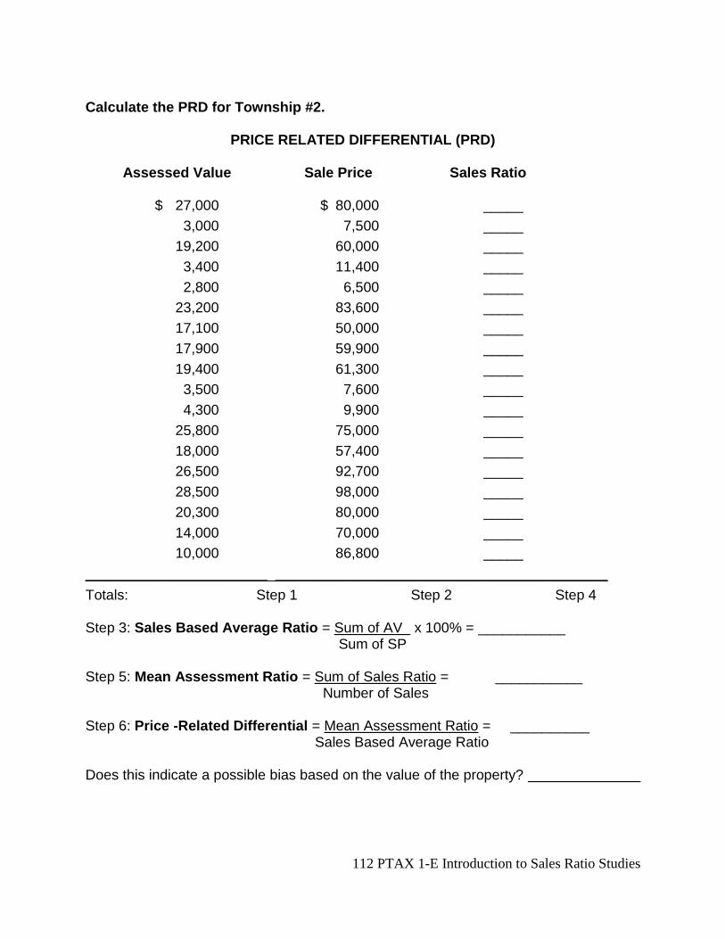
112 PTAX 1-E Introduction to Sales Ratio Studies
Calculate the PRD for Township #2.
PRICE RELATED DIFFERENTIAL (PRD)
Assessed Value Sale Price Sales Ratio $ 27,000 $ 80,000 _____
3,000 7,500 _____
19,200 60,000 _____
3,400 11,400 _____
2,800 6,500 _____
23,200 83,600 _____
17,100 50,000 _____
17,900 59,900 _____
19,400 61,300 _____
3,500 7,600 _____
4,300 9,900 _____
25,800 75,000 _____
18,000 57,400 _____
26,500 92,700 _____
28,500 98,000 _____
20,300 80,000 _____
14,000 70,000 _____
10,000 86,800 _____
__________________________________________________________________
Totals: Step 1 Step 2 Step 4
Step 3: Sales Based Average Ratio = Sum of AV x 100% = ___________ Sum of SP Step 5: Mean Assessment Ratio = Sum of Sales Ratio = ___________ Number of Sales Step 6: Price -Related Differential = Mean Assessment Ratio = __________ Sales Based Average Ratio Does this indicate a possible bias based on the value of the property?
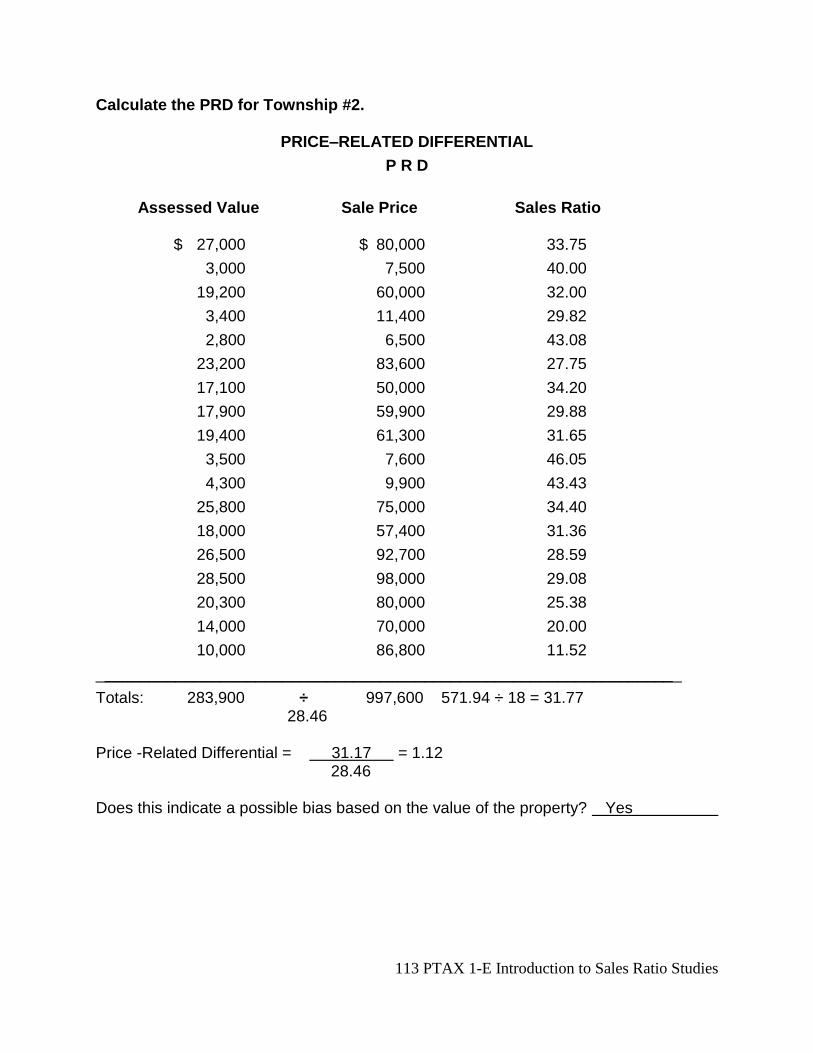
113 PTAX 1-E Introduction to Sales Ratio Studies
Calculate the PRD for Township #2.
PRICE–RELATED DIFFERENTIAL
P R D
Assessed Value Sale Price Sales Ratio
$ 27,000 $ 80,000 33.75
3,000 7,500 40.00
19,200 60,000 32.00
3,400 11,400 29.82
2,800 6,500 43.08
23,200 83,600 27.75
17,100 50,000 34.20
17,900 59,900 29.88
19,400 61,300 31.65
3,500 7,600 46.05
4,300 9,900 43.43
25,800 75,000 34.40
18,000 57,400 31.36
26,500 92,700 28.59
28,500 98,000 29.08
20,300 80,000 25.38
14,000 70,000 20.00
10,000 86,800 11.52
__________________________________________________________________
Totals: 283,900 ÷ 997,600 571.94 ÷ 18 = 31.77 28.46
Price -Related Differential = 31.17 = 1.12 28.46 Does this indicate a possible bias based on the value of the property? Yes
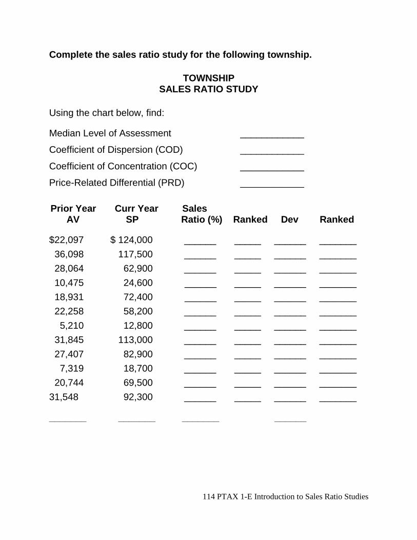
114 PTAX 1-E Introduction to Sales Ratio Studies
Complete the sales ratio study for the following township.
TOWNSHIP SALES RATIO STUDY
Using the chart below, find:
Median Level of Assessment ____________
Coefficient of Dispersion (COD) ____________
Coefficient of Concentration (COC) ____________
Price-Related Differential (PRD) ____________
Prior Year Curr Year Sales AV SP Ratio (%) Ranked Dev Ranked
$22,097 $ 124,000 ______ _____ ______ _______
36,098 117,500 ______ _____ ______ _______
28,064 62,900 ______ _____ ______ _______
10,475 24,600 ______ _____ ______ _______
18,931 72,400 ______ _____ ______ _______
22,258 58,200 ______ _____ ______ _______
5,210 12,800 ______ _____ ______ _______
31,845 113,000 ______ _____ ______ _______
27,407 82,900 ______ _____ ______ _______
7,319 18,700 ______ _____ ______ _______
20,744 69,500 ______ _____ ______ _______
31,548 92,300 ______ _____ ______ _______
_______ _______ _______ ______
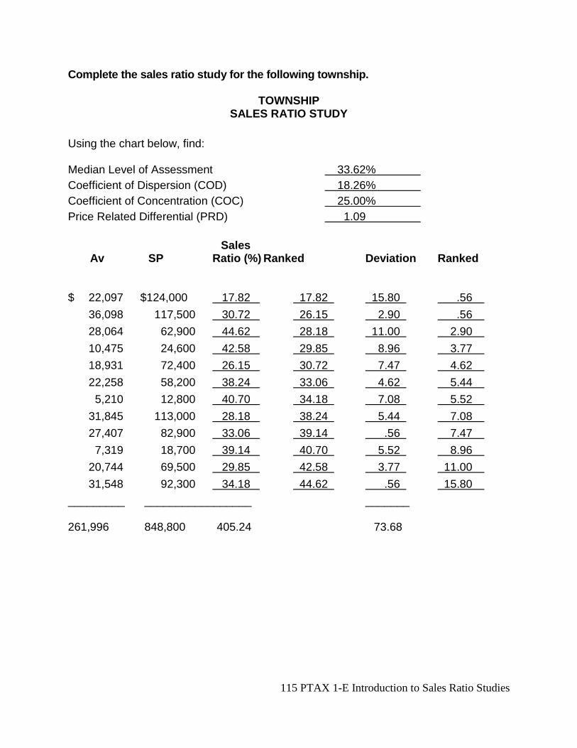
115 PTAX 1-E Introduction to Sales Ratio Studies
Complete the sales ratio study for the following township.
TOWNSHIP SALES RATIO STUDY
Using the chart below, find:
Median Level of Assessment 33.62%
Coefficient of Dispersion (COD) 18.26%
Coefficient of Concentration (COC) 25.00%
Price Related Differential (PRD) 1.09
Sales Av SP Ratio (%) Ranked Deviation Ranked
$ 22,097 $124,000 17.82 17.82 15.80 .56
36,098 117,500 30.72 26.15 2.90 .56
28,064 62,900 44.62 28.18 11.00 2.90
10,475 24,600 42.58 29.85 8.96 3.77
18,931 72,400 26.15 30.72 7.47 4.62
22,258 58,200 38.24 33.06 4.62 5.44
5,210 12,800 40.70 34.18 7.08 5.52
31,845 113,000 28.18 38.24 5.44 7.08
27,407 82,900 33.06 39.14 .56 7.47
7,319 18,700 39.14 40.70 5.52 8.96
20,744 69,500 29.85 42.58 3.77 11.00
31,548 92,300 34.18 44.62 .56 15.80
_________ _________________ _______ 261,996 848,800 405.24 73.68
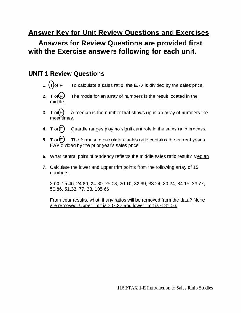
116 PTAX 1-E Introduction to Sales Ratio Studies
Answer Key for Unit Review Questions and Exercises
Answers for Review Questions are provided first with the Exercise answers following for each unit. UNIT 1 Review Questions
1. T or F To calculate a sales ratio, the EAV is divided by the sales price.
2. T or F The mode for an array of numbers is the result located in the
middle.
3. T or F A median is the number that shows up in an array of numbers the most times.
4. T or F Quartile ranges play no significant role in the sales ratio process.
5. T or F The formula to calculate a sales ratio contains the current year’s
EAV divided by the prior year’s sales price.
6. What central point of tendency reflects the middle sales ratio result? Median
7. Calculate the lower and upper trim points from the following array of 15 numbers.
2.00, 15.46, 24.80, 24.80, 25.08, 26.10, 32.99, 33.24, 33.24, 34.15, 36.77, 50.86, 51.33, 77. 33, 105.66
From your results, what, if any ratios will be removed from the data? None are removed. Upper limit is 207.22 and lower limit is -131.56.
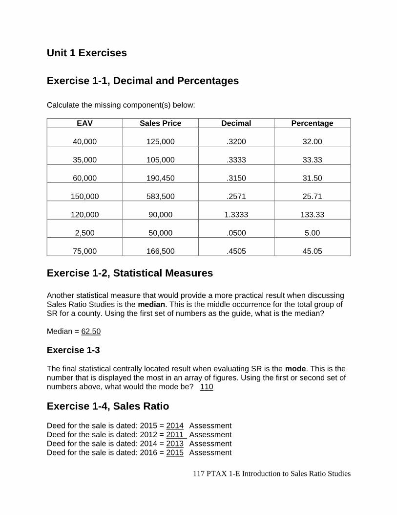
117 PTAX 1-E Introduction to Sales Ratio Studies
Unit 1 Exercises
Exercise 1-1, Decimal and Percentages
Calculate the missing component(s) below:
EAV Sales Price Decimal Percentage
40,000
125,000
.3200
32.00
35,000
105,000
.3333
33.33
60,000
190,450
.3150
31.50
150,000
583,500
.2571
25.71
120,000
90,000
1.3333
133.33
2,500
50,000
.0500
5.00
75,000
166,500
.4505
45.05
Exercise 1-2, Statistical Measures Another statistical measure that would provide a more practical result when discussing Sales Ratio Studies is the median. This is the middle occurrence for the total group of SR for a county. Using the first set of numbers as the guide, what is the median? Median = 62.50
Exercise 1-3 The final statistical centrally located result when evaluating SR is the mode. This is the number that is displayed the most in an array of figures. Using the first or second set of numbers above, what would the mode be? 110
Exercise 1-4, Sales Ratio Deed for the sale is dated: 2015 = 2014 Assessment Deed for the sale is dated: 2012 = 2011 Assessment Deed for the sale is dated: 2014 = 2013 Assessment Deed for the sale is dated: 2016 = 2015 Assessment
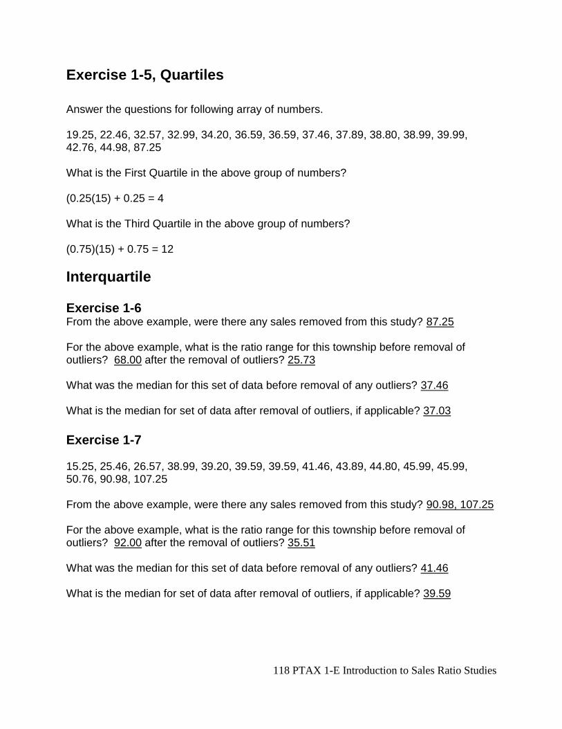
118 PTAX 1-E Introduction to Sales Ratio Studies
Exercise 1-5, Quartiles
Answer the questions for following array of numbers. 19.25, 22.46, 32.57, 32.99, 34.20, 36.59, 36.59, 37.46, 37.89, 38.80, 38.99, 39.99, 42.76, 44.98, 87.25 What is the First Quartile in the above group of numbers? (0.25(15) + 0.25 = 4 What is the Third Quartile in the above group of numbers? (0.75)(15) + 0.75 = 12
Interquartile
Exercise 1-6
From the above example, were there any sales removed from this study? 87.25 For the above example, what is the ratio range for this township before removal of outliers? 68.00 after the removal of outliers? 25.73 What was the median for this set of data before removal of any outliers? 37.46 What is the median for set of data after removal of outliers, if applicable? 37.03
Exercise 1-7 15.25, 25.46, 26.57, 38.99, 39.20, 39.59, 39.59, 41.46, 43.89, 44.80, 45.99, 45.99, 50.76, 90.98, 107.25 From the above example, were there any sales removed from this study? 90.98, 107.25 For the above example, what is the ratio range for this township before removal of outliers? 92.00 after the removal of outliers? 35.51 What was the median for this set of data before removal of any outliers? 41.46 What is the median for set of data after removal of outliers, if applicable? 39.59
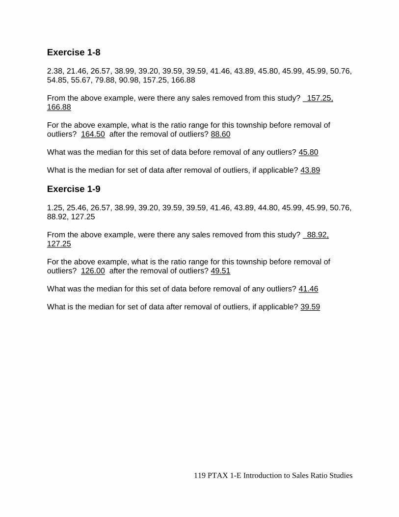
119 PTAX 1-E Introduction to Sales Ratio Studies
Exercise 1-8
2.38, 21.46, 26.57, 38.99, 39.20, 39.59, 39.59, 41.46, 43.89, 45.80, 45.99, 45.99, 50.76, 54.85, 55.67, 79.88, 90.98, 157.25, 166.88 From the above example, were there any sales removed from this study? 157.25, 166.88 For the above example, what is the ratio range for this township before removal of outliers? 164.50 after the removal of outliers? 88.60 What was the median for this set of data before removal of any outliers? 45.80 What is the median for set of data after removal of outliers, if applicable? 43.89
Exercise 1-9
1.25, 25.46, 26.57, 38.99, 39.20, 39.59, 39.59, 41.46, 43.89, 44.80, 45.99, 45.99, 50.76, 88.92, 127.25 From the above example, were there any sales removed from this study? 88.92, 127.25 For the above example, what is the ratio range for this township before removal of outliers? 126.00 after the removal of outliers? 49.51 What was the median for this set of data before removal of any outliers? 41.46 What is the median for set of data after removal of outliers, if applicable? 39.59
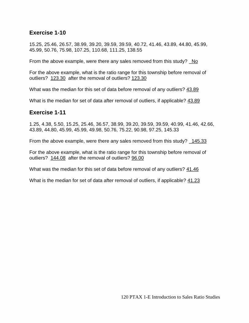
120 PTAX 1-E Introduction to Sales Ratio Studies
Exercise 1-10
15.25, 25.46, 26.57, 38.99, 39.20, 39.59, 39.59, 40.72, 41.46, 43.89, 44.80, 45.99, 45.99, 50.76, 75.98, 107.25, 110.68, 111.25, 138.55 From the above example, were there any sales removed from this study? No For the above example, what is the ratio range for this township before removal of outliers? 123.30 after the removal of outliers? 123.30 What was the median for this set of data before removal of any outliers? 43.89 What is the median for set of data after removal of outliers, if applicable? 43.89
Exercise 1-11
1.25, 4.38, 5.50, 15.25, 25.46, 36.57, 38.99, 39.20, 39.59, 39.59, 40.99, 41.46, 42.66, 43.89, 44.80, 45.99, 45.99, 49.98, 50.76, 75.22, 90.98, 97.25, 145.33 From the above example, were there any sales removed from this study? 145.33 For the above example, what is the ratio range for this township before removal of outliers? 144.08 after the removal of outliers? 96.00 What was the median for this set of data before removal of any outliers? 41.46 What is the median for set of data after removal of outliers, if applicable? 41.23
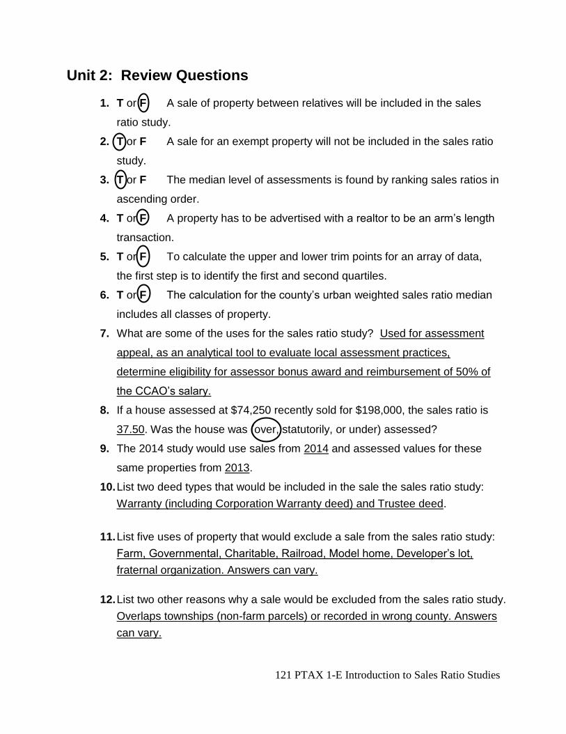
121 PTAX 1-E Introduction to Sales Ratio Studies
Unit 2: Review Questions
1. T or F A sale of property between relatives will be included in the sales
ratio study.
2. T or F A sale for an exempt property will not be included in the sales ratio
study.
3. T or F The median level of assessments is found by ranking sales ratios in
ascending order.
4. T or F A property has to be advertised with a realtor to be an arm’s length
transaction.
5. T or F To calculate the upper and lower trim points for an array of data,
the first step is to identify the first and second quartiles.
6. T or F The calculation for the county’s urban weighted sales ratio median
includes all classes of property.
7. What are some of the uses for the sales ratio study? Used for assessment
appeal, as an analytical tool to evaluate local assessment practices,
determine eligibility for assessor bonus award and reimbursement of 50% of
the CCAO’s salary.
8. If a house assessed at $74,250 recently sold for $198,000, the sales ratio is
37.50. Was the house was (over, statutorily, or under) assessed?
9. The 2014 study would use sales from 2014 and assessed values for these
same properties from 2013.
10. List two deed types that would be included in the sale the sales ratio study:
Warranty (including Corporation Warranty deed) and Trustee deed.
11. List five uses of property that would exclude a sale from the sales ratio study:
Farm, Governmental, Charitable, Railroad, Model home, Developer’s lot,
fraternal organization. Answers can vary.
12. List two other reasons why a sale would be excluded from the sales ratio study.
Overlaps townships (non-farm parcels) or recorded in wrong county. Answers
can vary.
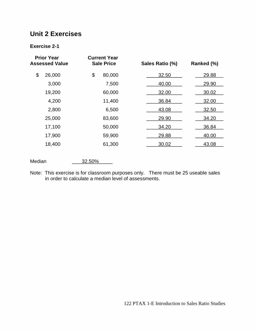
122 PTAX 1-E Introduction to Sales Ratio Studies
Unit 2 Exercises Exercise 2-1 Prior Year Current Year Assessed Value Sale Price Sales Ratio (%) Ranked (%) $ 26,000 $ 80,000 32.50 29.88
3,000 7,500 40.00 29.90
19,200 60,000 32.00 30.02
4,200 11,400 36.84 32.00
2,800 6,500 43.08 32.50
25,000 83,600 29.90 34.20
17,100 50,000 34.20 36.84
17,900 59,900 29.88 40.00
18,400 61,300 30.02 43.08
Median 32.50% Note: This exercise is for classroom purposes only. There must be 25 useable sales
in order to calculate a median level of assessments.
123 PTAX 1-E Introduction to Sales Ratio Studies
Exercise 2-2 Prior year Current Year Sales Assessed Value Sale Price Ratio Ranked $ 10,000 86,800 11.52 11.52
15,600 70,000 22.29 22.29
20,300 80,000 25.38 25.38
26,000 80,000 32.50 28.75
3,000 7,500 40.00 29.08
19,200 60,000 32.00 29.34
4,200 11,400 36.84 29.88
2,800 6,500 43.08 29.90
25,000 83,600 29.90 30.02
17,100 50,000 34.20 32.00
17,900 59,900 29.88 32.50
18,400 61,300 30.02 34.20
3,500 7,600 46.05 34.40
4,300 9,900 43.43 36.84
25,800 75,000 34.40 40.00
16,500 57,400 28.75 43.08
27,200 92,700 29.34 43.43
28,500 98,000 29.08 46.05
Median = 31.01%
Exercise 2-3 28.75, 29.08, 29.34, 29.88, 29.90, 30.02, 32.00, 32.50, 34.20, 34.40, 36.84, 40.00, 43.08, 43.43, 46.05 Median level of assessments (from above set of data) 32.50 First Quartile 29.88 Third Quartile 40.00 Lower trim point -30.84 Upper trim point 100.72 Median level of assessments after trimming 32.50
124 PTAX 1-E Introduction to Sales Ratio Studies
Urban Weighted Median Ratio In order to calculate a county median, it is necessary to know both the total assessed values in the county and the total market value of property in the county. What class of properties are included for the assessed values? Non-farm properties such as residential, commercial, industrial and other land/improvements.
Exercise 2-4 Assessed Value Median Ratio Estimated Full (000’s) (%) Value (000’s) Township 1 3,648 32.50 11,225 Township 2 10,450 33.10 31,571 Township 3 6,279 31.62 19,858 All other townships 30,560 32.20 94,907 Total 50,937 32.33 157,561 Urban weighted ratio – County’s Median Level of Assessments 32.33 Exercise 2-5 Assessed Value Median Ratio Estimated Full (000’s) (%) Value (000’s) Township 1 5,700 32.50 17,538 Township 2 12,555 33.10 37,931 Township 3 7,859 31.62 24,855 Township 4 14,667 34.88 42,050 Township 5 22,885 29.44 77,734 All other townships 30,560 32.81 93,142 Total 94,226 32.13 293,250 Urban weighted ratio – County’s Median Level of Assessments 32.13
125 PTAX 1-E Introduction to Sales Ratio Studies
Exercise 2-6 Assessed Value Median Ratio Estimated Full (000’s) (%) Value (000’s) Township 1 6,500 32.50 20,000 Township 2 14,887 33.10 44,976 Township 3 9,534 31.62 30,152 Township 4 20.080 34.88 57,569 Township 5 62,331 29.44 211,722 All other townships 46,788 32.81 142,603 Total 160,120 31.58 507,022 Urban weighted ratio – County’s Median Level of Assessments 31.58
126 PTAX 1-E Introduction to Sales Ratio Studies
Unit 3 Review Questions
1. T or F Individual sales that are clustered around a township’s median indicates a high COD result.
2. T or F A lower COC result indicates an issue with uniformity assessment.
3. T or F A PRD of 1.05 indicates a bias for assessments for higher-valued properties to be assessed higher than lower-valued properties.
4. Calculate the COD, COC and PRD for the following set of data:
ASSESSED SALES SALES VALUE PRICE RATIO RANKED MEDIAN DEVIATION $ 4,000 16,000 25.00 21.15 33.51 8.51
2,000 7,600 26.32 22.22 33.51 7.19
13,000 32,000 40.63 24.82 33.51 7.12
8,000 29,500 27.12 25.00 33.51 6.39
5,000 18,800 26.60 26.32 33.51 6.91
3,500 14,100 24.82 26.60 33.51 8.69
14,700 35,800 41.06 26.60 33.51 7.55
2,200 10,400 21.15 26.67 33.51 12.36
8,000 30,000 26.67 27.12 33.51 6.84
2,200 9,900 22.22 28.06 33.51 11.29
19,400 54,000 35.93 30.51 33.51 2.42
8,700 31,000 28.06 31.09 33.51 5.45
8,300 26,700 31.09 35.93 33.51 2.42
3,600 11,800 30.51 37.95 33.51 3.00
19,500 47,300 41.23 40.31 33.51 7.72
9,700 23,200 41.81 40.63 33.51 8.30
3,100 7,500 41.33 41.06 33.51 7.82
18,500 45,900 40.31 41.23 33.51 6.80
12,000 25,000 48.00 41.33 33.51 14.49
20,000 52,700 37.95 41.81 33.51 4.44
4,100 8,000 51.25 48.00 33.51 17.74
25,200 51,700 48.74 48.08 33.51 15.23
5,000 10,400 48.08 48.74 33.51 14.57
13,300 50,000 26.60 51.25 33.51 6.91
_______ ________ _______ _________
233,000 649,300 832.48 200.16
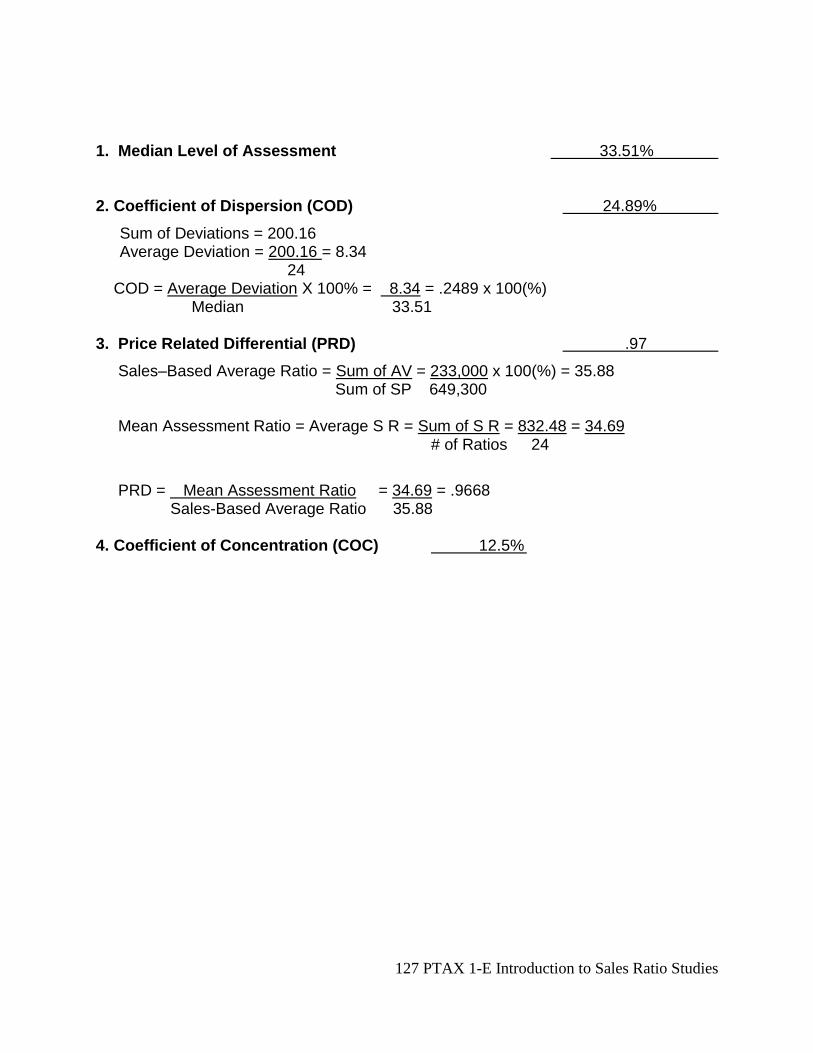
127 PTAX 1-E Introduction to Sales Ratio Studies
1. Median Level of Assessment 33.51%
2. Coefficient of Dispersion (COD) 24.89%
Sum of Deviations = 200.16 Average Deviation = 200.16 = 8.34 24 COD = Average Deviation X 100% = 8.34 = .2489 x 100(%) Median 33.51 3. Price Related Differential (PRD) .97
Sales–Based Average Ratio = Sum of AV = 233,000 x 100(%) = 35.88 Sum of SP 649,300 Mean Assessment Ratio = Average S R = Sum of S R = 832.48 = 34.69 # of Ratios 24
PRD = Mean Assessment Ratio = 34.69 = .9668 Sales-Based Average Ratio 35.88 4. Coefficient of Concentration (COC) 12.5%
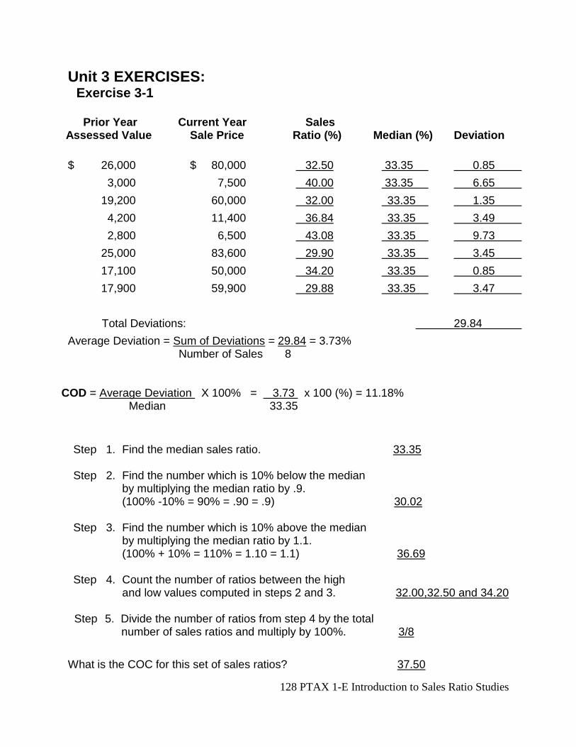
128 PTAX 1-E Introduction to Sales Ratio Studies
Unit 3 EXERCISES: Exercise 3-1
Prior Year Current Year Sales Assessed Value Sale Price Ratio (%) Median (%) Deviation
$ 26,000 $ 80,000 32.50 33.35 0.85
3,000 7,500 40.00 33.35 6.65
19,200 60,000 32.00 33.35 1.35
4,200 11,400 36.84 33.35 3.49
2,800 6,500 43.08 33.35 9.73
25,000 83,600 29.90 33.35 3.45
17,100 50,000 34.20 33.35 0.85
17,900 59,900 29.88 33.35 3.47
Total Deviations: 29.84
Average Deviation = Sum of Deviations = 29.84 = 3.73% Number of Sales 8
COD = Average Deviation X 100% = 3.73 x 100 (%) = 11.18% Median 33.35
Step 1. Find the median sales ratio. 33.35 Step 2. Find the number which is 10% below the median
by multiplying the median ratio by .9. (100% -10% = 90% = .90 = .9) 30.02
Step 3. Find the number which is 10% above the median
by multiplying the median ratio by 1.1. (100% + 10% = 110% = 1.10 = 1.1) 36.69
Step 4. Count the number of ratios between the high
and low values computed in steps 2 and 3. 32.00,32.50 and 34.20
Step 5. Divide the number of ratios from step 4 by the total number of sales ratios and multiply by 100%. 3/8
What is the COC for this set of sales ratios? 37.50
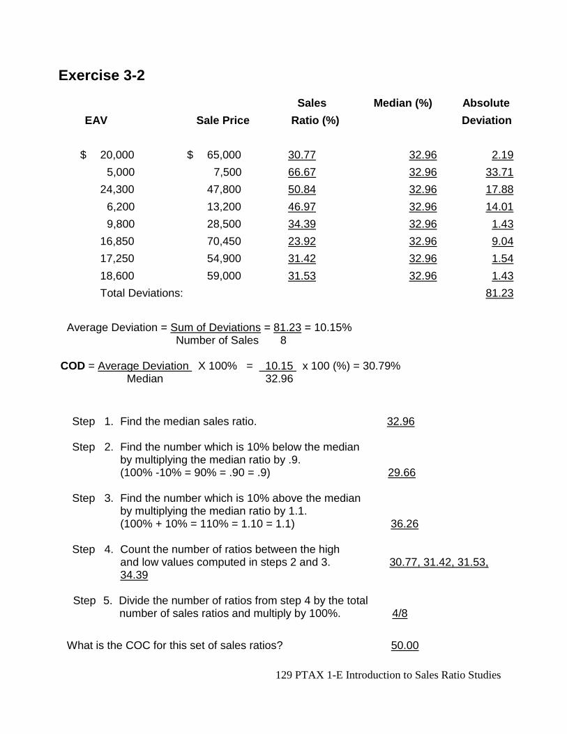
129 PTAX 1-E Introduction to Sales Ratio Studies
Exercise 3-2
Sales Median (%) Absolute
EAV Sale Price Ratio (%) Deviation
$ 20,000 $ 65,000 30.77 32.96 2.19
5,000 7,500 66.67 32.96 33.71
24,300 47,800 50.84 32.96 17.88
6,200 13,200 46.97 32.96 14.01
9,800 28,500 34.39 32.96 1.43
16,850 70,450 23.92 32.96 9.04
17,250 54,900 31.42 32.96 1.54
18,600 59,000 31.53 32.96 1.43
Total Deviations: 81.23
Average Deviation = Sum of Deviations = 81.23 = 10.15% Number of Sales 8
COD = Average Deviation X 100% = 10.15 x 100 (%) = 30.79% Median 32.96
Step 1. Find the median sales ratio. 32.96 Step 2. Find the number which is 10% below the median
by multiplying the median ratio by .9. (100% -10% = 90% = .90 = .9) 29.66
Step 3. Find the number which is 10% above the median
by multiplying the median ratio by 1.1. (100% + 10% = 110% = 1.10 = 1.1) 36.26
Step 4. Count the number of ratios between the high
and low values computed in steps 2 and 3. 30.77, 31.42, 31.53, 34.39
Step 5. Divide the number of ratios from step 4 by the total number of sales ratios and multiply by 100%. 4/8
What is the COC for this set of sales ratios? 50.00
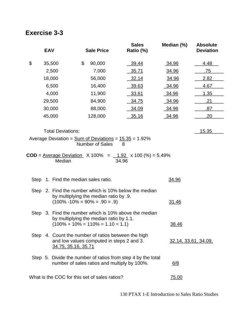
130 PTAX 1-E Introduction to Sales Ratio Studies
Exercise 3-3 Sales Median (%) Absolute EAV Sale Price Ratio (%) Deviation
$ 35,500 $ 90,000 39.44 34.96 4.48
2,500 7,000 35.71 34.96 .75
18,000 56,000 32.14 34.96 2.82
6,500 16,400 39.63 34.96 4.67
4,000 11,900 33.61 34.96 1.35
29,500 84,900 34.75 34.96 .21
30,000 88,000 34.09 34.96 .87
45,000 128,000 35.16 34.96 .20
Total Deviations: 15.35
Average Deviation = Sum of Deviations = 15.35 = 1.92% Number of Sales 8
COD = Average Deviation X 100% = 1.92 x 100 (%) = 5.49% Median 34.96
Step 1. Find the median sales ratio. 34.96 Step 2. Find the number which is 10% below the median
by multiplying the median ratio by .9. (100% -10% = 90% = .90 = .9) 31.46
Step 3. Find the number which is 10% above the median
by multiplying the median ratio by 1.1. (100% + 10% = 110% = 1.10 = 1.1) 38.46
Step 4. Count the number of ratios between the high
and low values computed in steps 2 and 3. 32.14, 33.61, 34.09, 34.75, 35.16, 35.71
Step 5. Divide the number of ratios from step 4 by the total number of sales ratios and multiply by 100%. 6/8
What is the COC for this set of sales ratios? 75.00
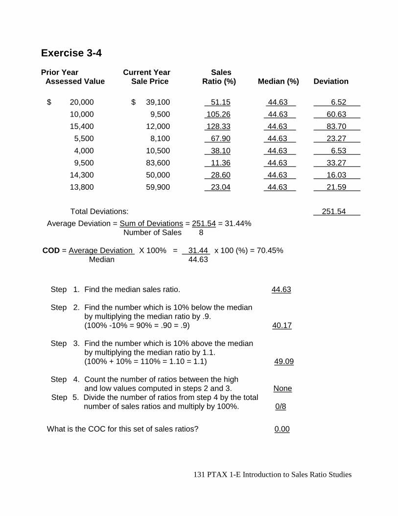
131 PTAX 1-E Introduction to Sales Ratio Studies
Exercise 3-4 Prior Year Current Year Sales Assessed Value Sale Price Ratio (%) Median (%) Deviation
$ 20,000 $ 39,100 51.15 44.63 6.52
10,000 9,500 105.26 44.63 60.63
15,400 12,000 128.33 44.63 83.70
5,500 8,100 67.90 44.63 23.27
4,000 10,500 38.10 44.63 6.53
9,500 83,600 11.36 44.63 33.27
14,300 50,000 28.60 44.63 16.03
13,800 59,900 23.04 44.63 21.59
Total Deviations: 251.54
Average Deviation = Sum of Deviations = 251.54 = 31.44% Number of Sales 8
COD = Average Deviation X 100% = 31.44 x 100 (%) = 70.45% Median 44.63
Step 1. Find the median sales ratio. 44.63 Step 2. Find the number which is 10% below the median
by multiplying the median ratio by .9. (100% -10% = 90% = .90 = .9) 40.17
Step 3. Find the number which is 10% above the median
by multiplying the median ratio by 1.1. (100% + 10% = 110% = 1.10 = 1.1) 49.09
Step 4. Count the number of ratios between the high
and low values computed in steps 2 and 3. None Step 5. Divide the number of ratios from step 4 by the total number of sales ratios and multiply by 100%. 0/8
What is the COC for this set of sales ratios? 0.00
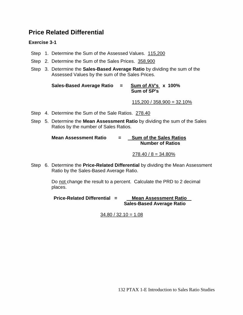
132 PTAX 1-E Introduction to Sales Ratio Studies
Price Related Differential
Exercise 3-1 Step 1. Determine the Sum of the Assessed Values. 115,200
Step 2. Determine the Sum of the Sales Prices. 358,900
Step 3. Determine the Sales-Based Average Ratio by dividing the sum of the Assessed Values by the sum of the Sales Prices. Sales-Based Average Ratio = Sum of AV's x 100% Sum of SP's 115,200 / 358,900 = 32.10%
Step 4. Determine the Sum of the Sale Ratios. 278.40
Step 5. Determine the Mean Assessment Ratio by dividing the sum of the Sales Ratios by the number of Sales Ratios. Mean Assessment Ratio = Sum of the Sales Ratios Number of Ratios 278.40 / 8 = 34.80%
Step 6. Determine the Price-Related Differential by dividing the Mean Assessment
Ratio by the Sales-Based Average Ratio. Do not change the result to a percent. Calculate the PRD to 2 decimal places.
Price-Related Differential = Mean Assessment Ratio
Sales-Based Average Ratio
34.80 / 32.10 = 1.08
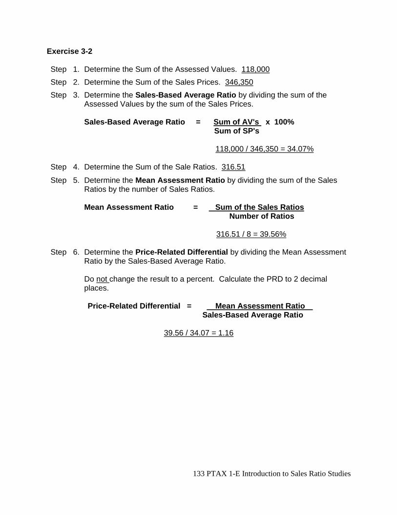
133 PTAX 1-E Introduction to Sales Ratio Studies
Exercise 3-2 Step 1. Determine the Sum of the Assessed Values. 118,000
Step 2. Determine the Sum of the Sales Prices. 346,350
Step 3. Determine the Sales-Based Average Ratio by dividing the sum of the Assessed Values by the sum of the Sales Prices. Sales-Based Average Ratio = Sum of AV's x 100% Sum of SP's 118,000 / 346,350 = 34.07%
Step 4. Determine the Sum of the Sale Ratios. 316.51
Step 5. Determine the Mean Assessment Ratio by dividing the sum of the Sales Ratios by the number of Sales Ratios. Mean Assessment Ratio = Sum of the Sales Ratios Number of Ratios 316.51 / 8 = 39.56%
Step 6. Determine the Price-Related Differential by dividing the Mean Assessment
Ratio by the Sales-Based Average Ratio. Do not change the result to a percent. Calculate the PRD to 2 decimal places.
Price-Related Differential = Mean Assessment Ratio
Sales-Based Average Ratio
39.56 / 34.07 = 1.16

134 PTAX 1-E Introduction to Sales Ratio Studies
Exercise 3-3 Step 1. Determine the Sum of the Assessed Values. 171,000
Step 2. Determine the Sum of the Sales Prices. 482,200
Step 3. Determine the Sales-Based Average Ratio by dividing the sum of the Assessed Values by the sum of the Sales Prices. Sales-Based Average Ratio = Sum of AV's x 100% Sum of SP's 171,000 / 482,200 = 35.46%
Step 4. Determine the Sum of the Sale Ratios. 284.53
Step 5. Determine the Mean Assessment Ratio by dividing the sum of the Sales Ratios by the number of Sales Ratios. Mean Assessment Ratio = Sum of the Sales Ratios Number of Ratios 284.53 / 8 = 35.57%
Step 6. Determine the Price-Related Differential by dividing the Mean Assessment
Ratio by the Sales-Based Average Ratio. Do not change the result to a percent. Calculate the PRD to 2 decimal places.
Price-Related Differential = Mean Assessment Ratio
Sales-Based Average Ratio
35.57 / 35.46 = 1.00
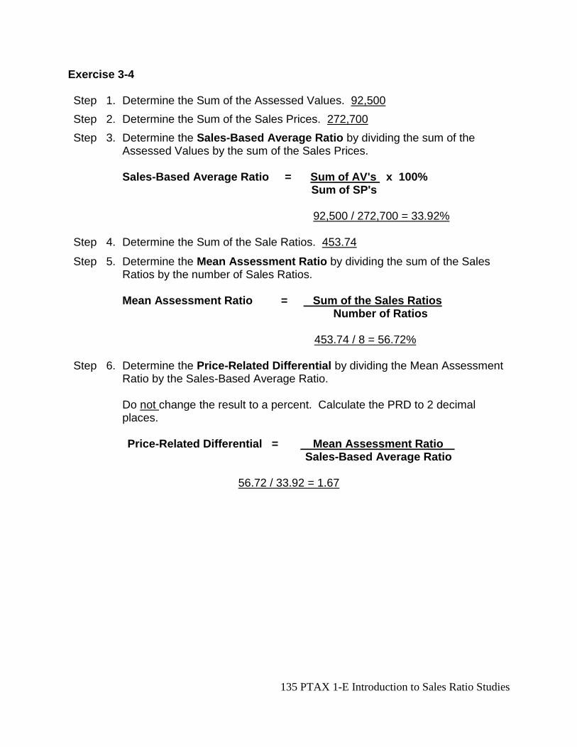
135 PTAX 1-E Introduction to Sales Ratio Studies
Exercise 3-4 Step 1. Determine the Sum of the Assessed Values. 92,500
Step 2. Determine the Sum of the Sales Prices. 272,700
Step 3. Determine the Sales-Based Average Ratio by dividing the sum of the Assessed Values by the sum of the Sales Prices. Sales-Based Average Ratio = Sum of AV's x 100% Sum of SP's 92,500 / 272,700 = 33.92%
Step 4. Determine the Sum of the Sale Ratios. 453.74
Step 5. Determine the Mean Assessment Ratio by dividing the sum of the Sales Ratios by the number of Sales Ratios. Mean Assessment Ratio = Sum of the Sales Ratios Number of Ratios 453.74 / 8 = 56.72%
Step 6. Determine the Price-Related Differential by dividing the Mean Assessment
Ratio by the Sales-Based Average Ratio. Do not change the result to a percent. Calculate the PRD to 2 decimal places.
Price-Related Differential = Mean Assessment Ratio
Sales-Based Average Ratio
56.72 / 33.92 = 1.67
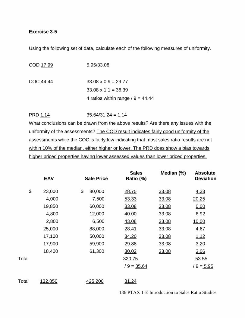
136 PTAX 1-E Introduction to Sales Ratio Studies
Exercise 3-5
Using the following set of data, calculate each of the following measures of uniformity.
COD 17.99 5.95/33.08
COC 44.44 33.08 x 0.9 = 29.77
33.08 x 1.1 = 36.39
4 ratios within range / 9 = 44.44
PRD 1.14 35.64/31.24 = 1.14
What conclusions can be drawn from the above results? Are there any issues with the
uniformity of the assessments? The COD result indicates fairly good uniformity of the
assessments while the COC is fairly low indicating that most sales ratio results are not
within 10% of the median, either higher or lower. The PRD does show a bias towards
higher priced properties having lower assessed values than lower priced properties.
Sales Median (%) Absolute EAV Sale Price Ratio (%) Deviation
$ 23,000 $ 80,000 28.75 33.08 4.33
4,000 7,500 53.33 33.08 20.25
19,850 60,000 33.08 33.08 0.00
4,800 12,000 40.00 33.08 6.92
2,800 6,500 43.08 33.08 10.00
25,000 88,000 28.41 33.08 4.67
17,100 50,000 34.20 33.08 1.12
17,900 59,900 29.88 33.08 3.20
18,400 61,300 30.02 33.08 3.06
Total 320.75 53.55
/ 9 = 35.64 / 9 = 5.95
Total 132,850 425,200 31.24
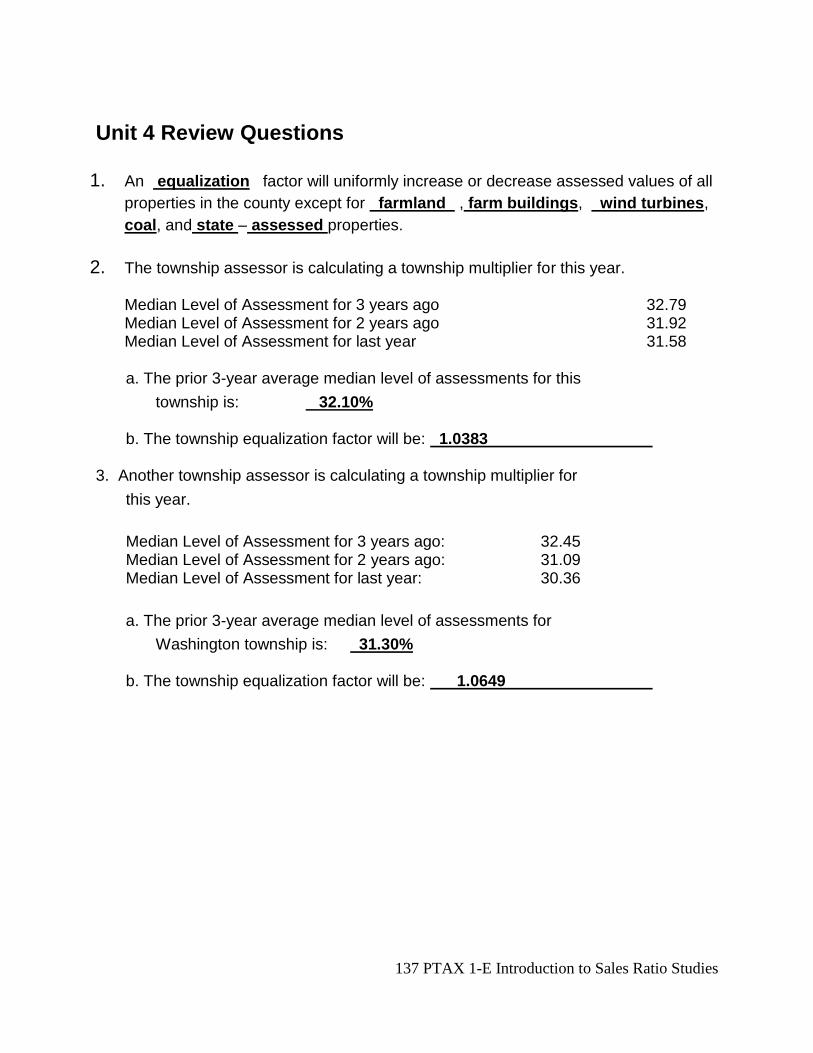
137 PTAX 1-E Introduction to Sales Ratio Studies
Unit 4 Review Questions
1. An equalization factor will uniformly increase or decrease assessed values of all
properties in the county except for farmland , farm buildings, wind turbines,
coal, and state – assessed properties.
2. The township assessor is calculating a township multiplier for this year. Median Level of Assessment for 3 years ago 32.79 Median Level of Assessment for 2 years ago 31.92 Median Level of Assessment for last year 31.58
a. The prior 3-year average median level of assessments for this
township is: 32.10% b. The township equalization factor will be: 1.0383 3. Another township assessor is calculating a township multiplier for
this year.
Median Level of Assessment for 3 years ago: 32.45 Median Level of Assessment for 2 years ago: 31.09 Median Level of Assessment for last year: 30.36
a. The prior 3-year average median level of assessments for
Washington township is: 31.30% b. The township equalization factor will be: 1.0649
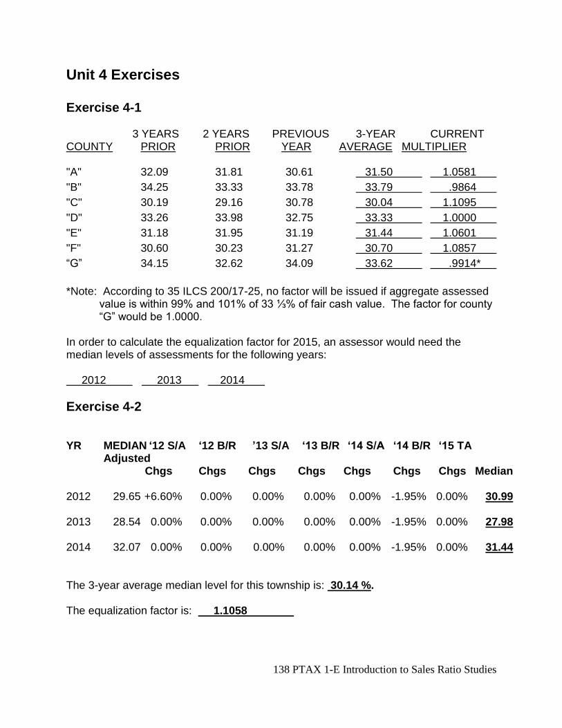
138 PTAX 1-E Introduction to Sales Ratio Studies
Unit 4 Exercises Exercise 4-1 3 YEARS 2 YEARS PREVIOUS 3-YEAR CURRENT COUNTY PRIOR PRIOR YEAR AVERAGE MULTIPLIER "A" 32.09 31.81 30.61 31.50 1.0581
"B" 34.25 33.33 33.78 33.79 .9864
"C" 30.19 29.16 30.78 30.04 1.1095
"D" 33.26 33.98 32.75 33.33 1.0000
"E" 31.18 31.95 31.19 31.44 1.0601
"F" 30.60 30.23 31.27 30.70 1.0857
“G” 34.15 32.62 34.09 33.62 .9914*
*Note: According to 35 ILCS 200/17-25, no factor will be issued if aggregate assessed
value is within 99% and 101% of 33 ⅓% of fair cash value. The factor for county “G” would be 1.0000.
In order to calculate the equalization factor for 2015, an assessor would need the median levels of assessments for the following years: 2012 2013 2014
Exercise 4-2 YR MEDIAN ‘12 S/A ‘12 B/R ’13 S/A ‘13 B/R ‘14 S/A ‘14 B/R ‘15 TA Adjusted Chgs Chgs Chgs Chgs Chgs Chgs Chgs Median 2012 29.65 +6.60% 0.00% 0.00% 0.00% 0.00% -1.95% 0.00% 30.99 2013 28.54 0.00% 0.00% 0.00% 0.00% 0.00% -1.95% 0.00% 27.98 2014 32.07 0.00% 0.00% 0.00% 0.00% 0.00% -1.95% 0.00% 31.44 The 3-year average median level for this township is: 30.14 %. The equalization factor is: 1.1058
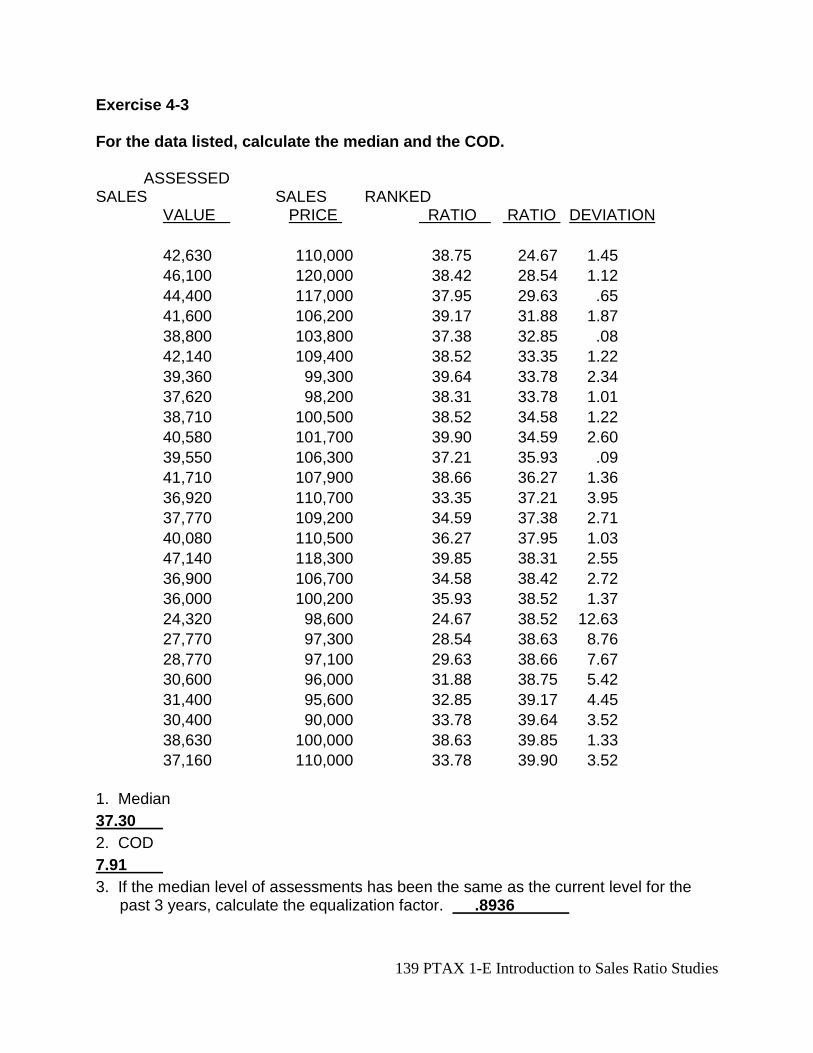
139 PTAX 1-E Introduction to Sales Ratio Studies
Exercise 4-3 For the data listed, calculate the median and the COD. ASSESSED SALES SALES RANKED VALUE PRICE RATIO RATIO DEVIATION
42,630 110,000 38.75 24.67 1.45
46,100 120,000 38.42 28.54 1.12
44,400 117,000 37.95 29.63 .65
41,600 106,200 39.17 31.88 1.87
38,800 103,800 37.38 32.85 .08
42,140 109,400 38.52 33.35 1.22
39,360 99,300 39.64 33.78 2.34
37,620 98,200 38.31 33.78 1.01
38,710 100,500 38.52 34.58 1.22
40,580 101,700 39.90 34.59 2.60
39,550 106,300 37.21 35.93 .09
41,710 107,900 38.66 36.27 1.36
36,920 110,700 33.35 37.21 3.95
37,770 109,200 34.59 37.38 2.71
40,080 110,500 36.27 37.95 1.03
47,140 118,300 39.85 38.31 2.55
36,900 106,700 34.58 38.42 2.72
36,000 100,200 35.93 38.52 1.37
24,320 98,600 24.67 38.52 12.63
27,770 97,300 28.54 38.63 8.76
28,770 97,100 29.63 38.66 7.67
30,600 96,000 31.88 38.75 5.42
31,400 95,600 32.85 39.17 4.45
30,400 90,000 33.78 39.64 3.52
38,630 100,000 38.63 39.85 1.33
37,160 110,000 33.78 39.90 3.52
1. Median
37.30
2. COD
7.91
3. If the median level of assessments has been the same as the current level for the past 3 years, calculate the equalization factor. .8936
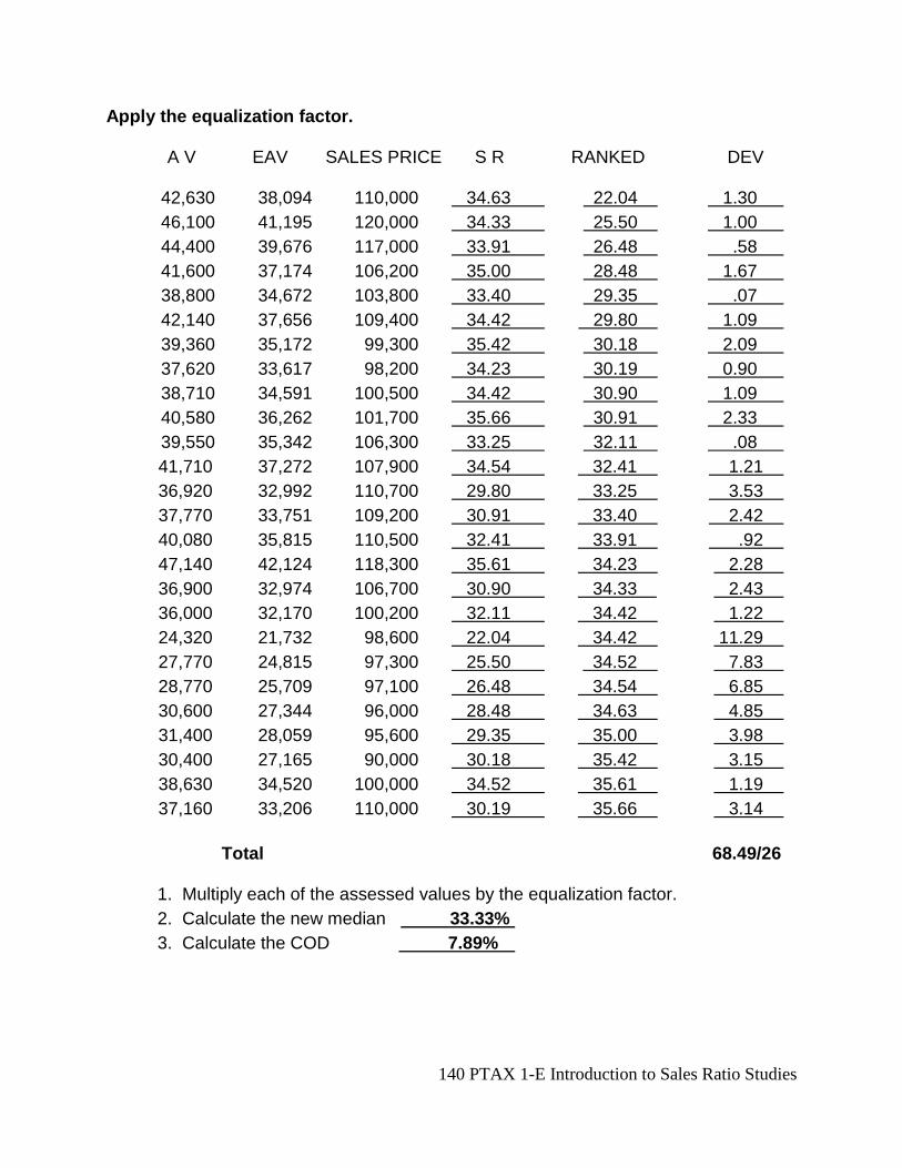
140 PTAX 1-E Introduction to Sales Ratio Studies
Apply the equalization factor. A V EAV SALES PRICE S R RANKED DEV 42,630 38,094 110,000 34.63 22.04 1.30
46,100 41,195 120,000 34.33 25.50 1.00
44,400 39,676 117,000 33.91 26.48 .58
41,600 37,174 106,200 35.00 28.48 1.67
38,800 34,672 103,800 33.40 29.35 .07
42,140 37,656 109,400 34.42 29.80 1.09
39,360 35,172 99,300 35.42 30.18 2.09
37,620 33,617 98,200 34.23 30.19 0.90
38,710 34,591 100,500 34.42 30.90 1.09
40,580 36,262 101,700 35.66 30.91 2.33
39,550 35,342 106,300 33.25 32.11 .08
41,710 37,272 107,900 34.54 32.41 1.21
36,920 32,992 110,700 29.80 33.25 3.53
37,770 33,751 109,200 30.91 33.40 2.42
40,080 35,815 110,500 32.41 33.91 .92
47,140 42,124 118,300 35.61 34.23 2.28
36,900 32,974 106,700 30.90 34.33 2.43
36,000 32,170 100,200 32.11 34.42 1.22
24,320 21,732 98,600 22.04 34.42 11.29
27,770 24,815 97,300 25.50 34.52 7.83
28,770 25,709 97,100 26.48 34.54 6.85
30,600 27,344 96,000 28.48 34.63 4.85
31,400 28,059 95,600 29.35 35.00 3.98
30,400 27,165 90,000 30.18 35.42 3.15
38,630 34,520 100,000 34.52 35.61 1.19
37,160 33,206 110,000 30.19 35.66 3.14
Total 68.49/26 1. Multiply each of the assessed values by the equalization factor.
2. Calculate the new median 33.33%
3. Calculate the COD 7.89%
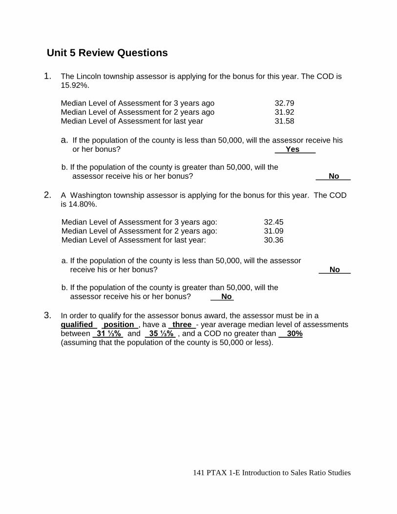
141 PTAX 1-E Introduction to Sales Ratio Studies
Unit 5 Review Questions
1. The Lincoln township assessor is applying for the bonus for this year. The COD is 15.92%. Median Level of Assessment for 3 years ago 32.79 Median Level of Assessment for 2 years ago 31.92 Median Level of Assessment for last year 31.58
a. If the population of the county is less than 50,000, will the assessor receive his or her bonus? Yes
b. If the population of the county is greater than 50,000, will the assessor receive his or her bonus? No
2. A Washington township assessor is applying for the bonus for this year. The COD is 14.80%.
Median Level of Assessment for 3 years ago: 32.45 Median Level of Assessment for 2 years ago: 31.09 Median Level of Assessment for last year: 30.36
a. If the population of the county is less than 50,000, will the assessor receive his or her bonus? No b. If the population of the county is greater than 50,000, will the assessor receive his or her bonus? No
3. In order to qualify for the assessor bonus award, the assessor must be in a qualified position , have a three - year average median level of assessments between 31 ⅓% and 35 ⅓% , and a COD no greater than 30% (assuming that the population of the county is 50,000 or less).
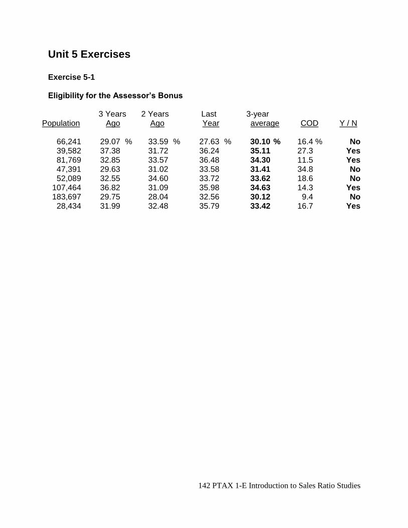
142 PTAX 1-E Introduction to Sales Ratio Studies
Unit 5 Exercises Exercise 5-1 Eligibility for the Assessor’s Bonus 3 Years 2 Years Last 3-year
Population Ago Ago Year average COD Y / N 66,241 29.07 % 33.59 % 27.63 % 30.10 % 16.4 % No 39,582 37.38 31.72 36.24 35.11 27.3 Yes 81,769 32.85 33.57 36.48 34.30 11.5 Yes 47,391 29.63 31.02 33.58 31.41 34.8 No 52,089 32.55 34.60 33.72 33.62 18.6 No 107,464 36.82 31.09 35.98 34.63 14.3 Yes 183,697 29.75 28.04 32.56 30.12 9.4 No 28,434 31.99 32.48 35.79 33.42 16.7 Yes
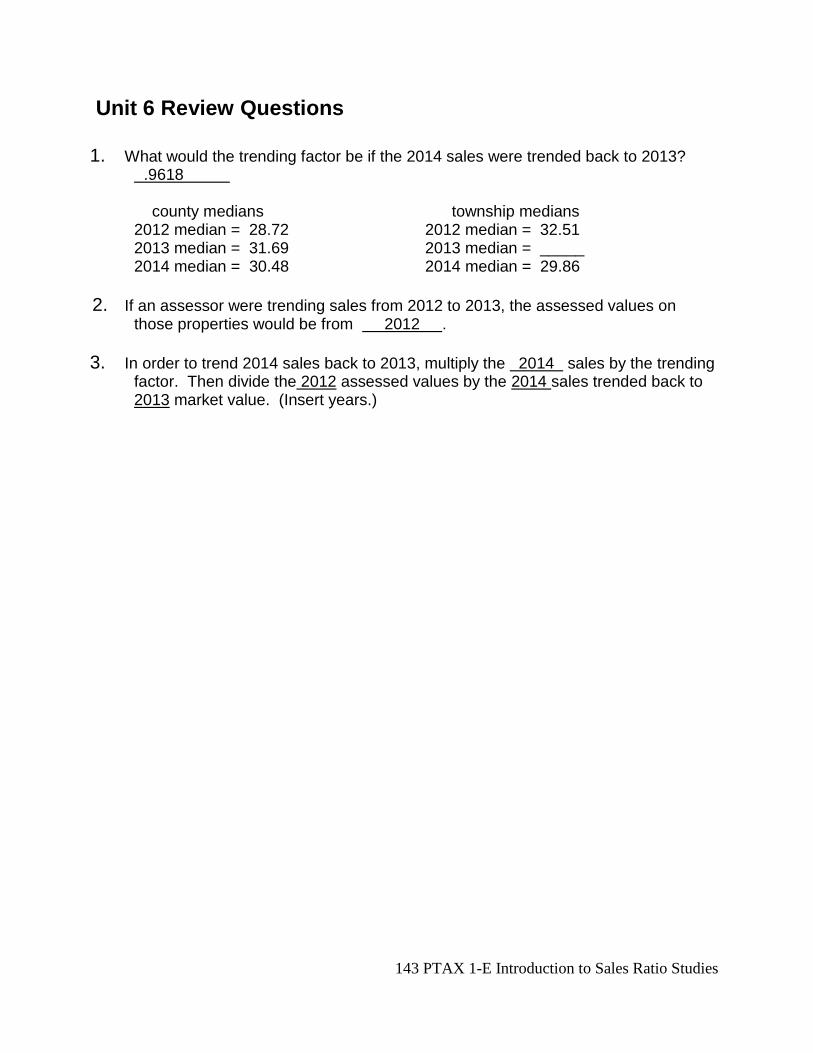
143 PTAX 1-E Introduction to Sales Ratio Studies
Unit 6 Review Questions
1. What would the trending factor be if the 2014 sales were trended back to 2013? .9618 county medians township medians 2012 median = 28.72 2012 median = 32.51 2013 median = 31.69 2013 median = _____ 2014 median = 30.48 2014 median = 29.86
2. If an assessor were trending sales from 2012 to 2013, the assessed values on those properties would be from 2012 .
3. In order to trend 2014 sales back to 2013, multiply the 2014 sales by the trending factor. Then divide the 2012 assessed values by the 2014 sales trended back to 2013 market value. (Insert years.)
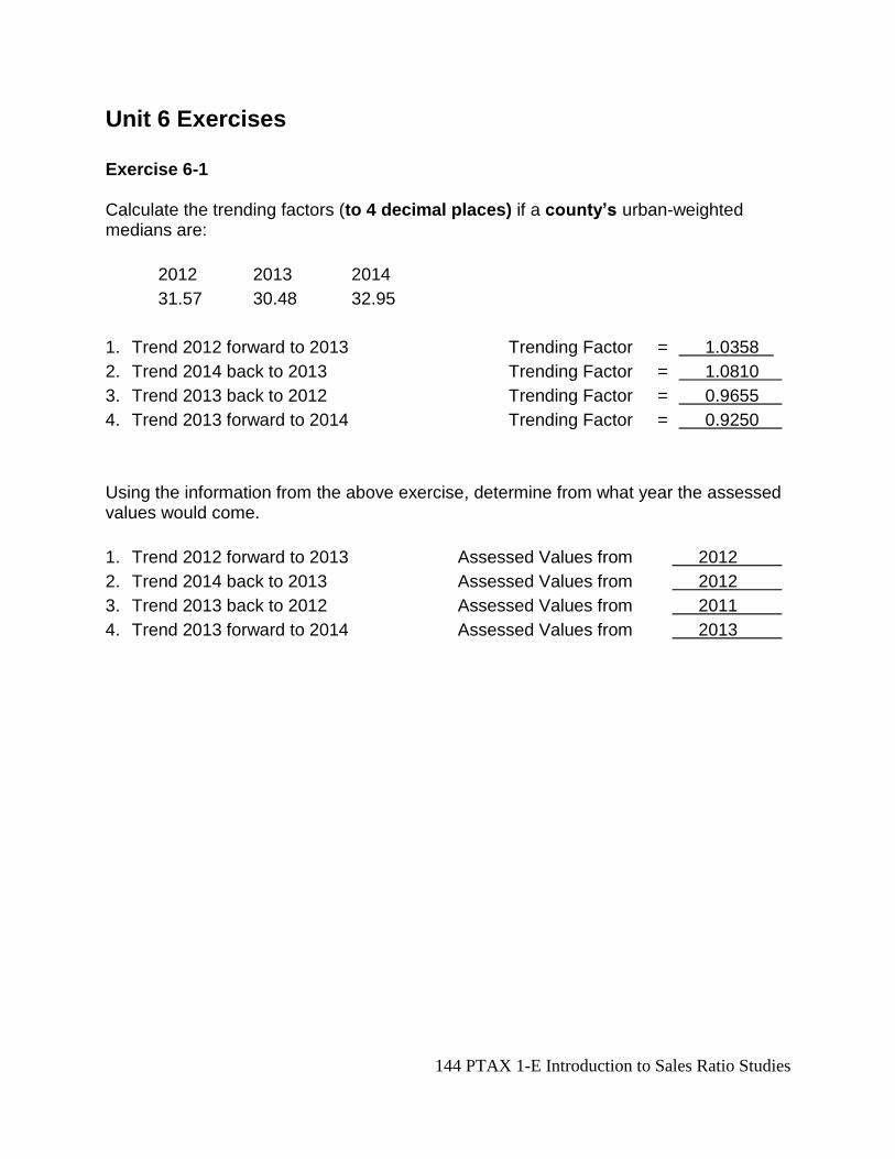
144 PTAX 1-E Introduction to Sales Ratio Studies
Unit 6 Exercises Exercise 6-1 Calculate the trending factors (to 4 decimal places) if a county’s urban-weighted medians are:
2012 2013 2014
31.57 30.48 32.95
1. Trend 2012 forward to 2013 Trending Factor = 1.0358
2. Trend 2014 back to 2013 Trending Factor = 1.0810
3. Trend 2013 back to 2012 Trending Factor = 0.9655
4. Trend 2013 forward to 2014 Trending Factor = 0.9250
Using the information from the above exercise, determine from what year the assessed values would come.
1. Trend 2012 forward to 2013 Assessed Values from 2012
2. Trend 2014 back to 2013 Assessed Values from 2012
3. Trend 2013 back to 2012 Assessed Values from 2011
4. Trend 2013 forward to 2014 Assessed Values from 2013
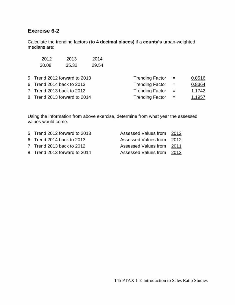
145 PTAX 1-E Introduction to Sales Ratio Studies
Exercise 6-2 Calculate the trending factors (to 4 decimal places) if a county’s urban-weighted medians are:
2012 2013 2014
30.08 35.32 29.54
5. Trend 2012 forward to 2013 Trending Factor = 0.8516
6. Trend 2014 back to 2013 Trending Factor = 0.8364
7. Trend 2013 back to 2012 Trending Factor = 1.1742
8. Trend 2013 forward to 2014 Trending Factor = 1.1957
Using the information from above exercise, determine from what year the assessed values would come.
5. Trend 2012 forward to 2013 Assessed Values from 2012
6. Trend 2014 back to 2013 Assessed Values from 2012
7. Trend 2013 back to 2012 Assessed Values from 2011
8. Trend 2013 forward to 2014 Assessed Values from 2013
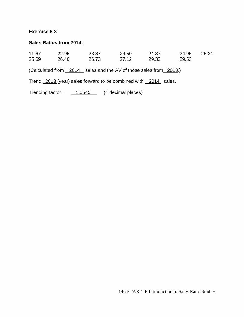
146 PTAX 1-E Introduction to Sales Ratio Studies
Exercise 6-3 Sales Ratios from 2014: 11.67 22.95 23.87 24.50 24.87 24.95 25.21 25.69 26.40 26.73 27.12 29.33 29.53 (Calculated from 2014 sales and the AV of those sales from 2013.) Trend 2013 (year) sales forward to be combined with 2014 sales. Trending factor = 1.0545 (4 decimal places)
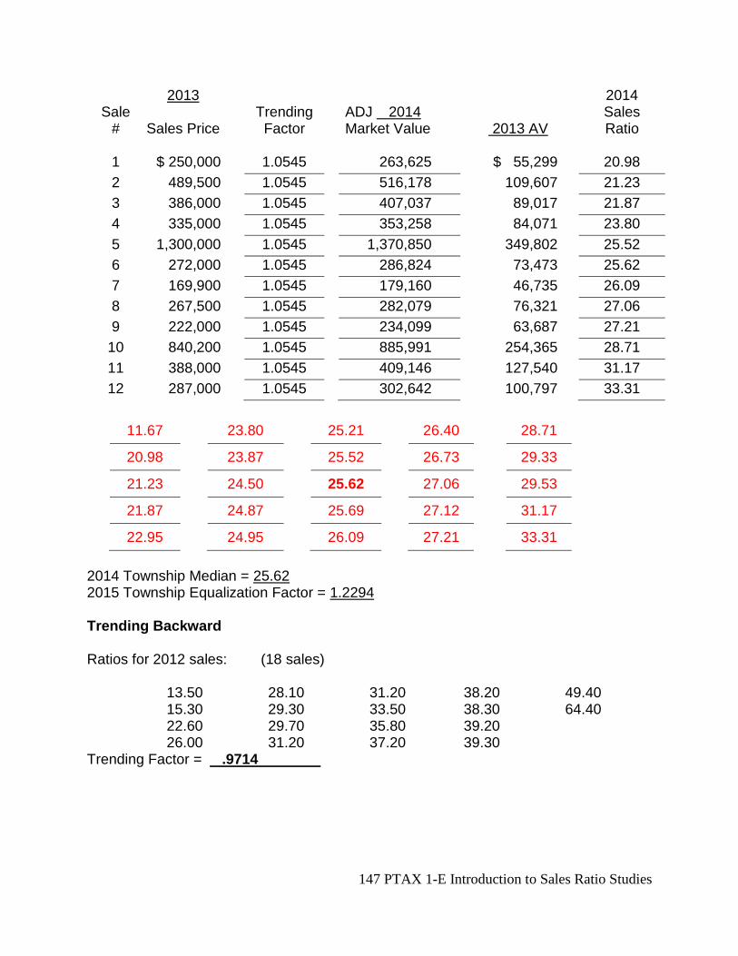
147 PTAX 1-E Introduction to Sales Ratio Studies
2013 2014 Sale
# Sales Price Trending
Factor ADJ 2014
Market Value 2013 AV Sales
Ratio
1 $ 250,000 1.0545 263,625 $ 55,299 20.98
2 489,500 1.0545 516,178 109,607 21.23
3 386,000 1.0545 407,037 89,017 21.87
4 335,000 1.0545 353,258 84,071 23.80
5 1,300,000 1.0545 1,370,850 349,802 25.52
6 272,000 1.0545 286,824 73,473 25.62
7 169,900 1.0545 179,160 46,735 26.09
8 267,500 1.0545 282,079 76,321 27.06
9 222,000 1.0545 234,099 63,687 27.21
10 840,200 1.0545 885,991 254,365 28.71
11 388,000 1.0545 409,146 127,540 31.17
12 287,000 1.0545 302,642 100,797 33.31
11.67 23.80 25.21 26.40 28.71
20.98 23.87 25.52 26.73 29.33
21.23 24.50 25.62 27.06 29.53
21.87 24.87 25.69 27.12 31.17
22.95 24.95 26.09 27.21 33.31
2014 Township Median = 25.62 2015 Township Equalization Factor = 1.2294 Trending Backward Ratios for 2012 sales: (18 sales) 13.50 28.10 31.20 38.20 49.40 15.30 29.30 33.50 38.30 64.40 22.60 29.70 35.80 39.20 26.00 31.20 37.20 39.30 Trending Factor = .9714
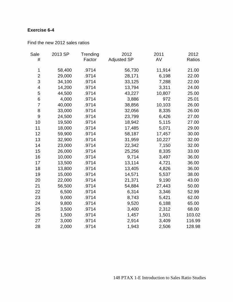
148 PTAX 1-E Introduction to Sales Ratio Studies
Exercise 6-4
Find the new 2012 sales ratios
Sale 2013 SP Trending 2012 2011 2012
# Factor Adjusted SP AV Ratios
1 58,400 .9714 56,730 11,914 21.00
2 29,000 .9714 28,171 6,198 22.00
3 34,100 .9714 33,125 7,288 22.00
4 14,200 .9714 13,794 3,311 24.00
5 44,500 .9714 43,227 10,807 25.00
6 4,000 .9714 3,886 972 25.01
7 40,000 .9714 38,856 10,103 26.00
8 33,000 .9714 32,056 8,335 26.00
9 24,500 .9714 23,799 6,426 27.00
10 19,500 .9714 18,942 5,115 27.00
11 18,000 .9714 17,485 5,071 29.00
12 59,900 .9714 58,187 17,457 30.00
13 32,900 .9714 31,959 10,227 32.00
14 23,000 .9714 22,342 7,150 32.00
15 26,000 .9714 25,256 8,335 33.00
16 10,000 .9714 9,714 3,497 36.00
17 13,500 .9714 13,114 4,721 36.00
18 13,800 .9714 13,405 4,826 36.00
19 15,000 .9714 14,571 5,537 38.00
20 22,000 .9714 21,371 9,190 43.00
21 56,500 .9714 54,884 27,443 50.00
22 6,500 .9714 6,314 3,346 52.99
23 9,000 .9714 8,743 5,421 62.00
24 9,800 .9714 9,520 6,188 65.00
25 3,500 .9714 3,400 2,312 68.00
26 1,500 .9714 1,457 1,501 103.02
27 3,000 .9714 2,914 3,409 116.99
28 2,000 .9714 1,943 2,506 128.98
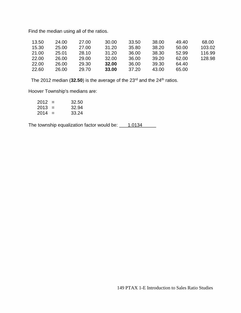
149 PTAX 1-E Introduction to Sales Ratio Studies
Find the median using all of the ratios. 13.50 24.00 27.00 30.00 33.50 38.00 49.40 68.00 15.30 25.00 27.00 31.20 35.80 38.20 50.00 103.02 21.00 25.01 28.10 31.20 36.00 38.30 52.99 116.99 22.00 26.00 29.00 32.00 36.00 39.20 62.00 128.98 22.00 26.00 29.30 32.00 36.00 39.30 64.40 22.60 26.00 29.70 33.00 37.20 43.00 65.00
The 2012 median (32.50) is the average of the 23rd and the 24th ratios. Hoover Township's medians are: 2012 = 32.50 2013 = 32.94 2014 = 33.24
The township equalization factor would be: 1.0134
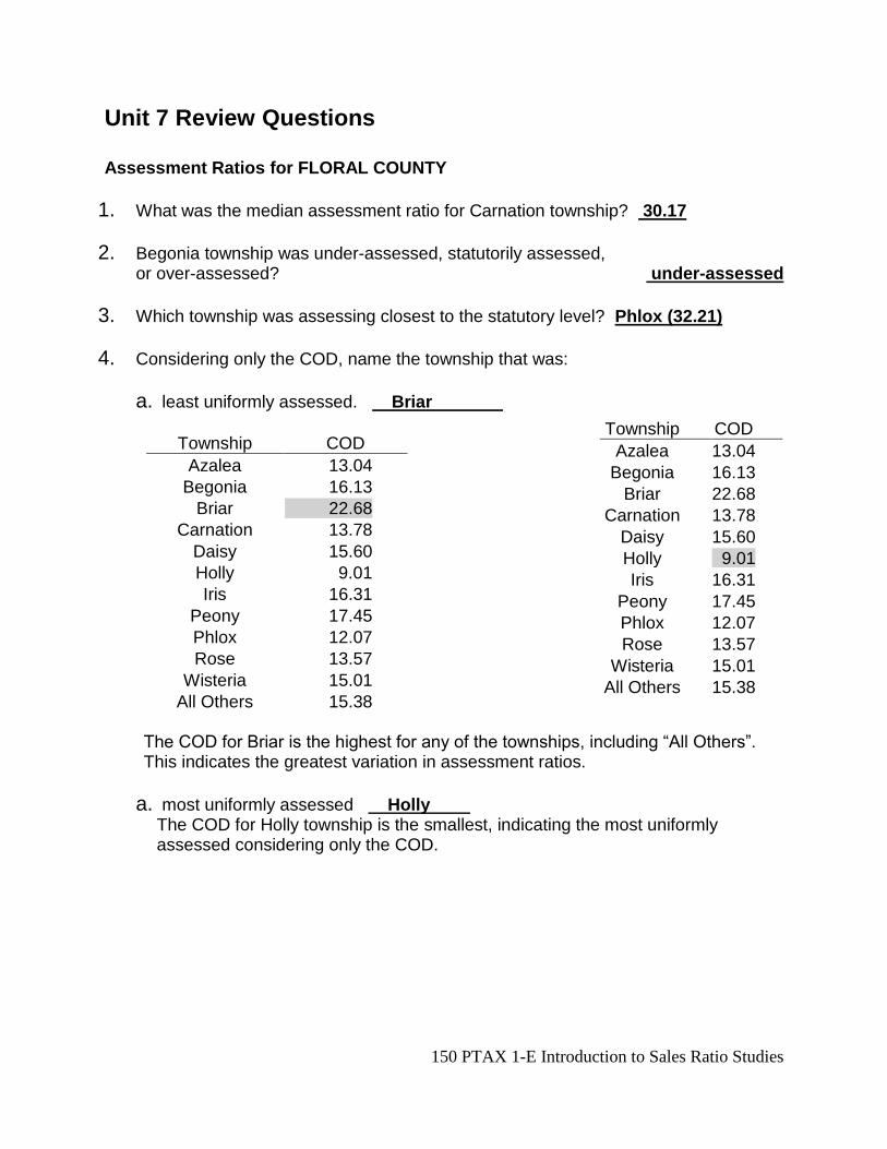
150 PTAX 1-E Introduction to Sales Ratio Studies
Unit 7 Review Questions Assessment Ratios for FLORAL COUNTY
1. What was the median assessment ratio for Carnation township? 30.17
2. Begonia township was under-assessed, statutorily assessed, or over-assessed? under-assessed
3. Which township was assessing closest to the statutory level? Phlox (32.21)
4. Considering only the COD, name the township that was:
a. least uniformly assessed. Briar
Township COD
Azalea 13.04
Begonia 16.13
Briar 22.68
Carnation 13.78
Daisy 15.60
Holly 9.01
Iris 16.31
Peony 17.45
Phlox 12.07
Rose 13.57
Wisteria 15.01
All Others 15.38 The COD for Briar is the highest for any of the townships, including “All Others”. This indicates the greatest variation in assessment ratios.
a. most uniformly assessed Holly The COD for Holly township is the smallest, indicating the most uniformly assessed considering only the COD.
Township COD
Azalea 13.04
Begonia 16.13
Briar 22.68
Carnation 13.78
Daisy 15.60
Holly 9.01
Iris 16.31
Peony 17.45
Phlox 12.07
Rose 13.57
Wisteria 15.01
All Others 15.38
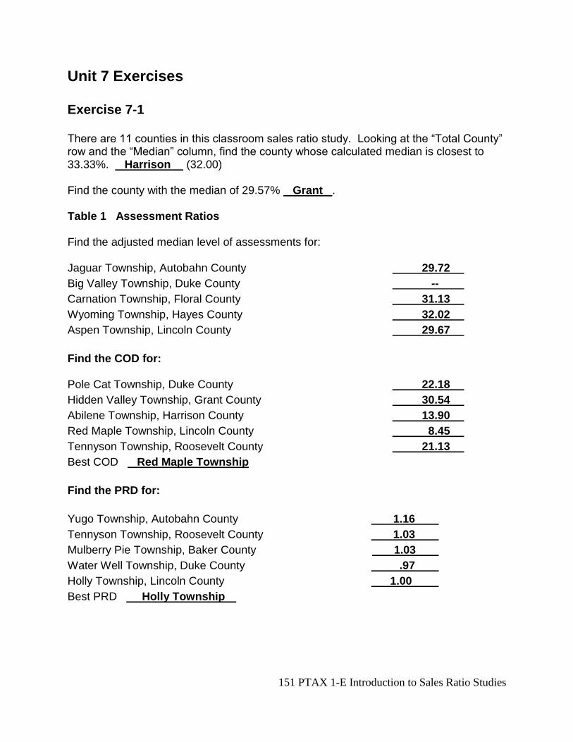
151 PTAX 1-E Introduction to Sales Ratio Studies
Unit 7 Exercises Exercise 7-1 There are 11 counties in this classroom sales ratio study. Looking at the “Total County” row and the “Median” column, find the county whose calculated median is closest to 33.33%. Harrison (32.00) Find the county with the median of 29.57% Grant . Table 1 Assessment Ratios Find the adjusted median level of assessments for: Jaguar Township, Autobahn County 29.72
Big Valley Township, Duke County --
Carnation Township, Floral County 31.13
Wyoming Township, Hayes County 32.02
Aspen Township, Lincoln County 29.67
Find the COD for: Pole Cat Township, Duke County 22.18
Hidden Valley Township, Grant County 30.54
Abilene Township, Harrison County 13.90
Red Maple Township, Lincoln County 8.45
Tennyson Township, Roosevelt County 21.13
Best COD Red Maple Township
Find the PRD for:
Yugo Township, Autobahn County 1.16
Tennyson Township, Roosevelt County 1.03
Mulberry Pie Township, Baker County 1.03
Water Well Township, Duke County .97
Holly Township, Lincoln County 1.00
Best PRD Holly Township
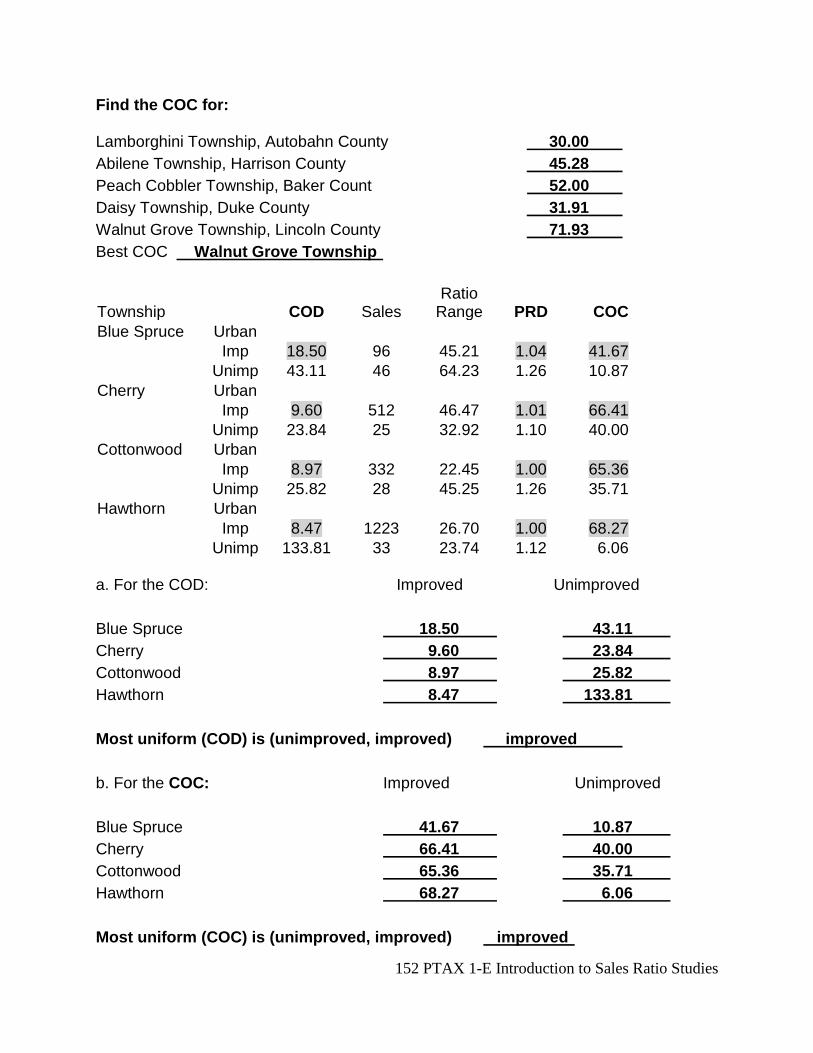
152 PTAX 1-E Introduction to Sales Ratio Studies
Find the COC for: Lamborghini Township, Autobahn County 30.00
Abilene Township, Harrison County 45.28
Peach Cobbler Township, Baker Count 52.00
Daisy Township, Duke County 31.91
Walnut Grove Township, Lincoln County 71.93
Best COC Walnut Grove Township
Township COD Sales Ratio
Range PRD COC
Blue Spruce Urban
Imp 18.50 96 45.21 1.04 41.67
Unimp 43.11 46 64.23 1.26 10.87
Cherry Urban
Imp 9.60 512 46.47 1.01 66.41
Unimp 23.84 25 32.92 1.10 40.00
Cottonwood Urban
Imp 8.97 332 22.45 1.00 65.36
Unimp 25.82 28 45.25 1.26 35.71
Hawthorn Urban
Imp 8.47 1223 26.70 1.00 68.27
Unimp 133.81 33 23.74 1.12 6.06 a. For the COD: Improved Unimproved
Blue Spruce 18.50 43.11
Cherry 9.60 23.84
Cottonwood 8.97 25.82
Hawthorn 8.47 133.81
Most uniform (COD) is (unimproved, improved) improved
b. For the COC: Improved Unimproved
Blue Spruce 41.67 10.87
Cherry 66.41 40.00
Cottonwood 65.36 35.71
Hawthorn 68.27 6.06
Most uniform (COC) is (unimproved, improved) improved
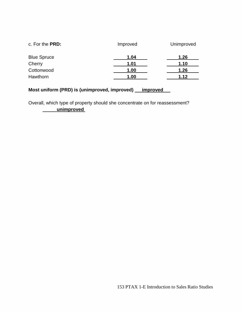
153 PTAX 1-E Introduction to Sales Ratio Studies
c. For the PRD: Improved Unimproved
Blue Spruce 1.04 1.26
Cherry 1.01 1.10
Cottonwood 1.00 1.26
Hawthorn 1.00 1.12
Most uniform (PRD) is (unimproved, improved) improved
Overall, which type of property should she concentrate on for reassessment?
unimproved
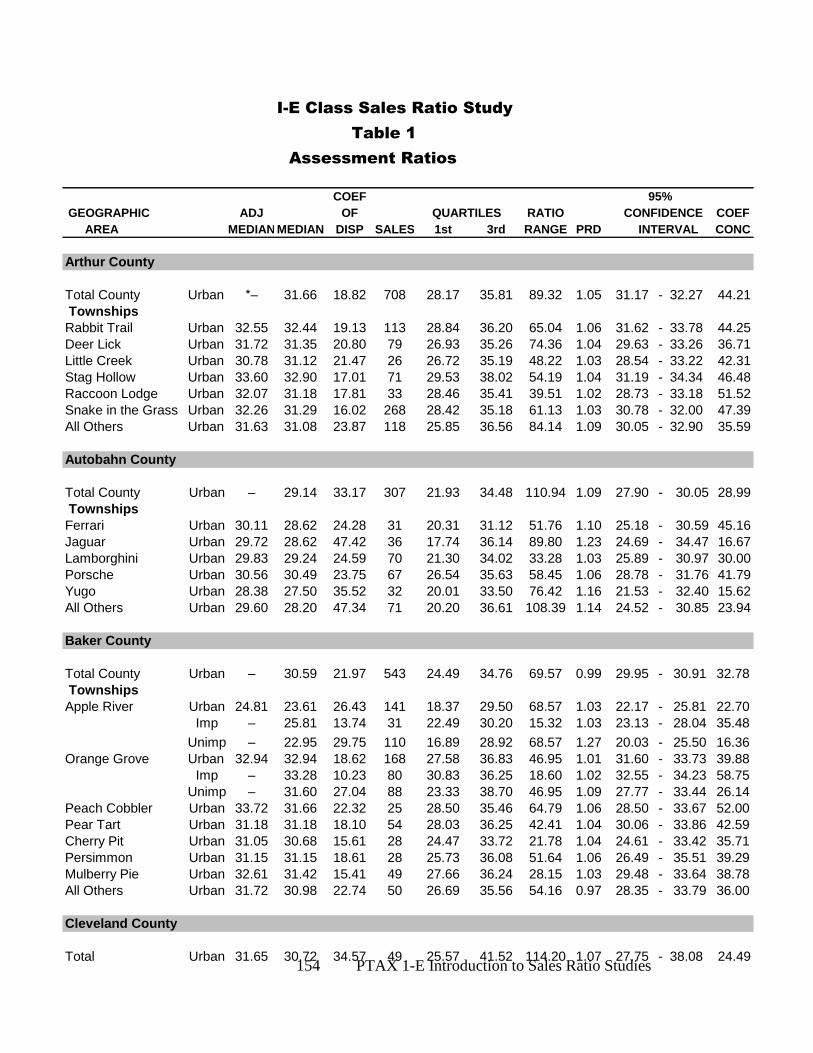
154 PTAX 1-E Introduction to Sales Ratio Studies
I-E Class Sales Ratio Study
Table 1
COEF
GEOGRAPHIC ADJ OF QUARTILES RATIO COEF
AREA MEDIAN MEDIAN DISP SALES 1st 3rd RANGE PRD CONC
Arthur County
Total County Urban *– 31.66 18.82 708 28.17 35.81 89.32 1.05 31.17 - 32.27 44.21
Townships
Rabbit Trail Urban 32.55 32.44 19.13 113 28.84 36.20 65.04 1.06 31.62 - 33.78 44.25
Deer Lick Urban 31.72 31.35 20.80 79 26.93 35.26 74.36 1.04 29.63 - 33.26 36.71
Little Creek Urban 30.78 31.12 21.47 26 26.72 35.19 48.22 1.03 28.54 - 33.22 42.31
Stag Hollow Urban 33.60 32.90 17.01 71 29.53 38.02 54.19 1.04 31.19 - 34.34 46.48
Raccoon Lodge Urban 32.07 31.18 17.81 33 28.46 35.41 39.51 1.02 28.73 - 33.18 51.52
Snake in the Grass Urban 32.26 31.29 16.02 268 28.42 35.18 61.13 1.03 30.78 - 32.00 47.39
All Others Urban 31.63 31.08 23.87 118 25.85 36.56 84.14 1.09 30.05 - 32.90 35.59
Autobahn County
Total County Urban – 29.14 33.17 307 21.93 34.48 110.94 1.09 27.90 - 30.05 28.99
Townships
Ferrari Urban 30.11 28.62 24.28 31 20.31 31.12 51.76 1.10 25.18 - 30.59 45.16
Jaguar Urban 29.72 28.62 47.42 36 17.74 36.14 89.80 1.23 24.69 - 34.47 16.67
Lamborghini Urban 29.83 29.24 24.59 70 21.30 34.02 33.28 1.03 25.89 - 30.97 30.00
Porsche Urban 30.56 30.49 23.75 67 26.54 35.63 58.45 1.06 28.78 - 31.76 41.79
Yugo Urban 28.38 27.50 35.52 32 20.01 33.50 76.42 1.16 21.53 - 32.40 15.62
All Others Urban 29.60 28.20 47.34 71 20.20 36.61 108.39 1.14 24.52 - 30.85 23.94
Baker County
Total County Urban – 30.59 21.97 543 24.49 34.76 69.57 0.99 29.95 - 30.91 32.78
Townships
Apple River Urban 24.81 23.61 26.43 141 18.37 29.50 68.57 1.03 22.17 - 25.81 22.70
Imp – 25.81 13.74 31 22.49 30.20 15.32 1.03 23.13 - 28.04 35.48
Unimp – 22.95 29.75 110 16.89 28.92 68.57 1.27 20.03 - 25.50 16.36
Orange Grove Urban 32.94 32.94 18.62 168 27.58 36.83 46.95 1.01 31.60 - 33.73 39.88
Imp – 33.28 10.23 80 30.83 36.25 18.60 1.02 32.55 - 34.23 58.75
Unimp – 31.60 27.04 88 23.33 38.70 46.95 1.09 27.77 - 33.44 26.14
Peach Cobbler Urban 33.72 31.66 22.32 25 28.50 35.46 64.79 1.06 28.50 - 33.67 52.00
Pear Tart Urban 31.18 31.18 18.10 54 28.03 36.25 42.41 1.04 30.06 - 33.86 42.59
Cherry Pit Urban 31.05 30.68 15.61 28 24.47 33.72 21.78 1.04 24.61 - 33.42 35.71
Persimmon Urban 31.15 31.15 18.61 28 25.73 36.08 51.64 1.06 26.49 - 35.51 39.29
Mulberry Pie Urban 32.61 31.42 15.41 49 27.66 36.24 28.15 1.03 29.48 - 33.64 38.78
All Others Urban 31.72 30.98 22.74 50 26.69 35.56 54.16 0.97 28.35 - 33.79 36.00
Cleveland County
Total Urban 31.65 30.72 34.57 49 25.57 41.52 114.20 1.07 27.75 - 38.08 24.49
Assessment Ratios
95%
CONFIDENCE
INTERVAL
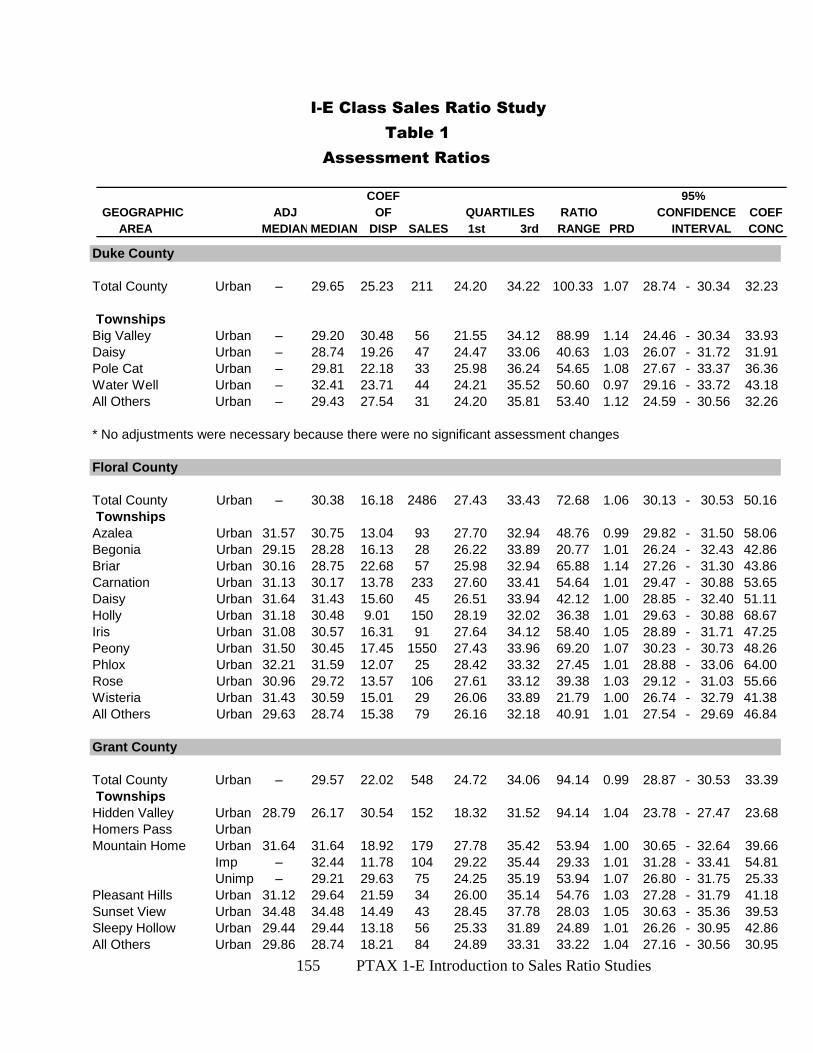
155 PTAX 1-E Introduction to Sales Ratio Studies
Duke County
Total County Urban – 29.65 25.23 211 24.20 34.22 100.33 1.07 28.74 - 30.34 32.23
Townships
Big Valley Urban – 29.20 30.48 56 21.55 34.12 88.99 1.14 24.46 - 30.34 33.93
Daisy Urban – 28.74 19.26 47 24.47 33.06 40.63 1.03 26.07 - 31.72 31.91
Pole Cat Urban – 29.81 22.18 33 25.98 36.24 54.65 1.08 27.67 - 33.37 36.36
Water Well Urban – 32.41 23.71 44 24.21 35.52 50.60 0.97 29.16 - 33.72 43.18
All Others Urban – 29.43 27.54 31 24.20 35.81 53.40 1.12 24.59 - 30.56 32.26
* No adjustments were necessary because there were no significant assessment changes
Floral County
Total County Urban – 30.38 16.18 2486 27.43 33.43 72.68 1.06 30.13 - 30.53 50.16
Townships
Azalea Urban 31.57 30.75 13.04 93 27.70 32.94 48.76 0.99 29.82 - 31.50 58.06
Begonia Urban 29.15 28.28 16.13 28 26.22 33.89 20.77 1.01 26.24 - 32.43 42.86
Briar Urban 30.16 28.75 22.68 57 25.98 32.94 65.88 1.14 27.26 - 31.30 43.86
Carnation Urban 31.13 30.17 13.78 233 27.60 33.41 54.64 1.01 29.47 - 30.88 53.65
Daisy Urban 31.64 31.43 15.60 45 26.51 33.94 42.12 1.00 28.85 - 32.40 51.11
Holly Urban 31.18 30.48 9.01 150 28.19 32.02 36.38 1.01 29.63 - 30.88 68.67
Iris Urban 31.08 30.57 16.31 91 27.64 34.12 58.40 1.05 28.89 - 31.71 47.25
Peony Urban 31.50 30.45 17.45 1550 27.43 33.96 69.20 1.07 30.23 - 30.73 48.26
Phlox Urban 32.21 31.59 12.07 25 28.42 33.32 27.45 1.01 28.88 - 33.06 64.00
Rose Urban 30.96 29.72 13.57 106 27.61 33.12 39.38 1.03 29.12 - 31.03 55.66
Wisteria Urban 31.43 30.59 15.01 29 26.06 33.89 21.79 1.00 26.74 - 32.79 41.38
All Others Urban 29.63 28.74 15.38 79 26.16 32.18 40.91 1.01 27.54 - 29.69 46.84
Grant County
Total County Urban – 29.57 22.02 548 24.72 34.06 94.14 0.99 28.87 - 30.53 33.39
Townships
Hidden Valley Urban 28.79 26.17 30.54 152 18.32 31.52 94.14 1.04 23.78 - 27.47 23.68
Homers Pass Urban
Mountain Home Urban 31.64 31.64 18.92 179 27.78 35.42 53.94 1.00 30.65 - 32.64 39.66
Imp – 32.44 11.78 104 29.22 35.44 29.33 1.01 31.28 - 33.41 54.81
Unimp – 29.21 29.63 75 24.25 35.19 53.94 1.07 26.80 - 31.75 25.33
Pleasant Hills Urban 31.12 29.64 21.59 34 26.00 35.14 54.76 1.03 27.28 - 31.79 41.18
Sunset View Urban 34.48 34.48 14.49 43 28.45 37.78 28.03 1.05 30.63 - 35.36 39.53
Sleepy Hollow Urban 29.44 29.44 13.18 56 25.33 31.89 24.89 1.01 26.26 - 30.95 42.86
All Others Urban 29.86 28.74 18.21 84 24.89 33.31 33.22 1.04 27.16 - 30.56 30.95
I-E Class Sales Ratio Study
Table 1
COEF
GEOGRAPHIC ADJ OF QUARTILES RATIO COEF
AREA MEDIAN MEDIAN DISP SALES 1st 3rd RANGE PRD CONC
Assessment Ratios
95%
CONFIDENCE
INTERVAL
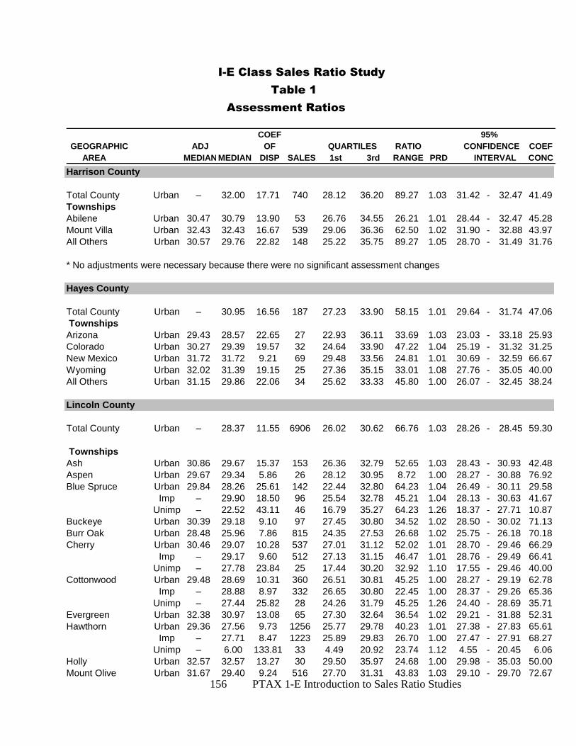
156 PTAX 1-E Introduction to Sales Ratio Studies
I-E Class Sales Ratio Study
Table 1
COEF
GEOGRAPHIC ADJ OF QUARTILES RATIO COEF
AREA MEDIAN MEDIAN DISP SALES 1st 3rd RANGE PRD CONC
Assessment Ratios
95%
CONFIDENCE
INTERVAL
Harrison County
Total County Urban – 32.00 17.71 740 28.12 36.20 89.27 1.03 31.42 - 32.47 41.49
Townships
Abilene Urban 30.47 30.79 13.90 53 26.76 34.55 26.21 1.01 28.44 - 32.47 45.28
Mount Villa Urban 32.43 32.43 16.67 539 29.06 36.36 62.50 1.02 31.90 - 32.88 43.97
All Others Urban 30.57 29.76 22.82 148 25.22 35.75 89.27 1.05 28.70 - 31.49 31.76
* No adjustments were necessary because there were no significant assessment changes
Hayes County
Total County Urban – 30.95 16.56 187 27.23 33.90 58.15 1.01 29.64 - 31.74 47.06
Townships
Arizona Urban 29.43 28.57 22.65 27 22.93 36.11 33.69 1.03 23.03 - 33.18 25.93
Colorado Urban 30.27 29.39 19.57 32 24.64 33.90 47.22 1.04 25.19 - 31.32 31.25
New Mexico Urban 31.72 31.72 9.21 69 29.48 33.56 24.81 1.01 30.69 - 32.59 66.67
Wyoming Urban 32.02 31.39 19.15 25 27.36 35.15 33.01 1.08 27.76 - 35.05 40.00
All Others Urban 31.15 29.86 22.06 34 25.62 33.33 45.80 1.00 26.07 - 32.45 38.24
Lincoln County
Total County Urban – 28.37 11.55 6906 26.02 30.62 66.76 1.03 28.26 - 28.45 59.30
Townships
Ash Urban 30.86 29.67 15.37 153 26.36 32.79 52.65 1.03 28.43 - 30.93 42.48
Aspen Urban 29.67 29.34 5.86 26 28.12 30.95 8.72 1.00 28.27 - 30.88 76.92
Blue Spruce Urban 29.84 28.26 25.61 142 22.44 32.80 64.23 1.04 26.49 - 30.11 29.58
Imp – 29.90 18.50 96 25.54 32.78 45.21 1.04 28.13 - 30.63 41.67
Unimp – 22.52 43.11 46 16.79 35.27 64.23 1.26 18.37 - 27.71 10.87
Buckeye Urban 30.39 29.18 9.10 97 27.45 30.80 34.52 1.02 28.50 - 30.02 71.13
Burr Oak Urban 28.48 25.96 7.86 815 24.35 27.53 26.68 1.02 25.75 - 26.18 70.18
Cherry Urban 30.46 29.07 10.28 537 27.01 31.12 52.02 1.01 28.70 - 29.46 66.29
Imp – 29.17 9.60 512 27.13 31.15 46.47 1.01 28.76 - 29.49 66.41
Unimp – 27.78 23.84 25 17.44 30.20 32.92 1.10 17.55 - 29.46 40.00
Cottonwood Urban 29.48 28.69 10.31 360 26.51 30.81 45.25 1.00 28.27 - 29.19 62.78
Imp – 28.88 8.97 332 26.65 30.80 22.45 1.00 28.37 - 29.26 65.36
Unimp – 27.44 25.82 28 24.26 31.79 45.25 1.26 24.40 - 28.69 35.71
Evergreen Urban 32.38 30.97 13.08 65 27.30 32.64 36.54 1.02 29.21 - 31.88 52.31
Hawthorn Urban 29.36 27.56 9.73 1256 25.77 29.78 40.23 1.01 27.38 - 27.83 65.61
Imp – 27.71 8.47 1223 25.89 29.83 26.70 1.00 27.47 - 27.91 68.27
Unimp – 6.00 133.81 33 4.49 20.92 23.74 1.12 4.55 - 20.45 6.06
Holly Urban 32.57 32.57 13.27 30 29.50 35.97 24.68 1.00 29.98 - 35.03 50.00
Mount Olive Urban 31.67 29.40 9.24 516 27.70 31.31 43.83 1.03 29.10 - 29.70 72.67
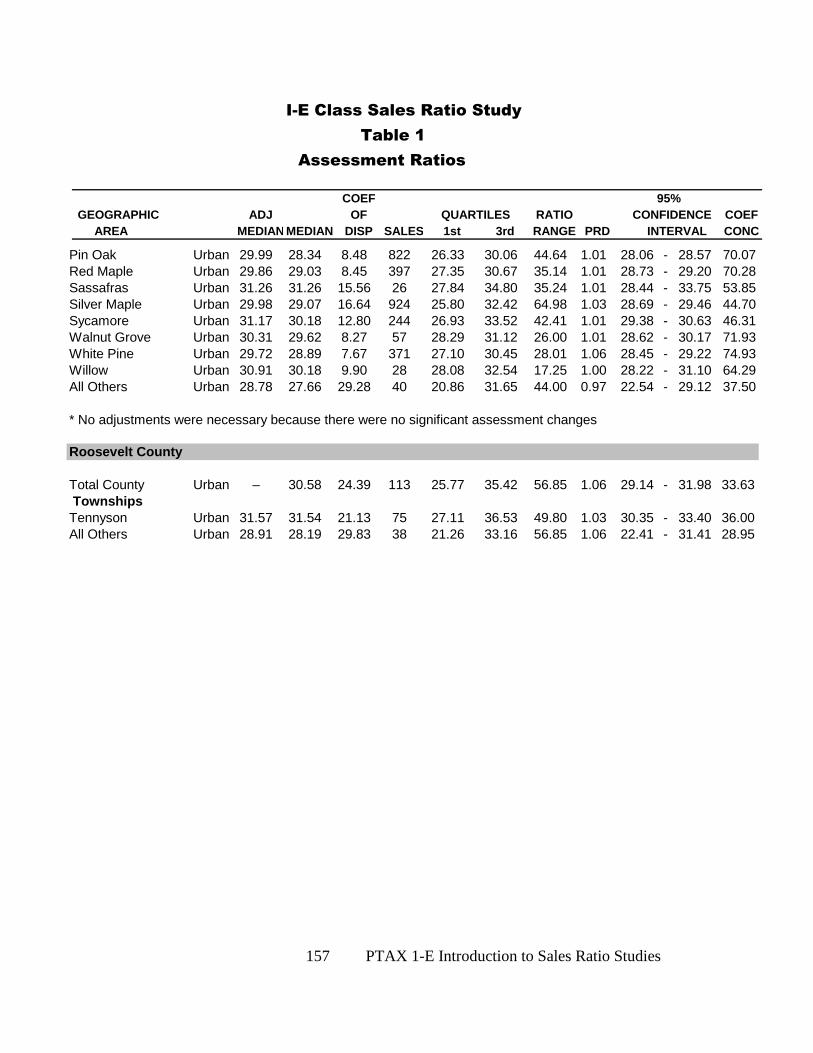
157 PTAX 1-E Introduction to Sales Ratio Studies
I-E Class Sales Ratio Study
Table 1
COEF
GEOGRAPHIC ADJ OF QUARTILES RATIO COEF
AREA MEDIAN MEDIAN DISP SALES 1st 3rd RANGE PRD CONC
Assessment Ratios
95%
CONFIDENCE
INTERVAL
Pin Oak Urban 29.99 28.34 8.48 822 26.33 30.06 44.64 1.01 28.06 - 28.57 70.07
Red Maple Urban 29.86 29.03 8.45 397 27.35 30.67 35.14 1.01 28.73 - 29.20 70.28
Sassafras Urban 31.26 31.26 15.56 26 27.84 34.80 35.24 1.01 28.44 - 33.75 53.85
Silver Maple Urban 29.98 29.07 16.64 924 25.80 32.42 64.98 1.03 28.69 - 29.46 44.70
Sycamore Urban 31.17 30.18 12.80 244 26.93 33.52 42.41 1.01 29.38 - 30.63 46.31
Walnut Grove Urban 30.31 29.62 8.27 57 28.29 31.12 26.00 1.01 28.62 - 30.17 71.93
White Pine Urban 29.72 28.89 7.67 371 27.10 30.45 28.01 1.06 28.45 - 29.22 74.93
Willow Urban 30.91 30.18 9.90 28 28.08 32.54 17.25 1.00 28.22 - 31.10 64.29
All Others Urban 28.78 27.66 29.28 40 20.86 31.65 44.00 0.97 22.54 - 29.12 37.50
* No adjustments were necessary because there were no significant assessment changes
Roosevelt County
Total County Urban – 30.58 24.39 113 25.77 35.42 56.85 1.06 29.14 - 31.98 33.63
Townships
Tennyson Urban 31.57 31.54 21.13 75 27.11 36.53 49.80 1.03 30.35 - 33.40 36.00
All Others Urban 28.91 28.19 29.83 38 21.26 33.16 56.85 1.06 22.41 - 31.41 28.95
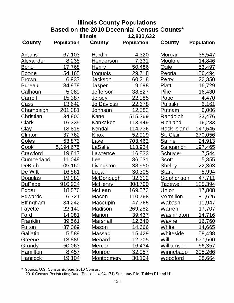
158
Illinois County Populations
Based on the 2010 Decennial Census Counts*
Illinois 12,830,632 County Population County Population County Population Adams 67,103 Hardin 4,320 Morgan 35,547 Alexander 8,238 Henderson 7,331 Moultrie 14,846 Bond 17,768 Henry 50,486 Ogle 53,497 Boone 54,165 Iroquois 29,718 Peoria 186,494 Brown 6,937 Jackson 60,218 Perry 22,350 Bureau 34,978 Jasper 9,698 Piatt 16,729 Calhoun 5,089 Jefferson 38,827 Pike 16,430 Carroll 15,387 Jersey 22,985 Pope 4,470 Cass 13,642 Jo Daviess 22,678 Pulaski 6,161 Champaign 201,081 Johnson 12,582 Putnam 6,006 Christian 34,800 Kane 515,269 Randolph 33,476 Clark 16,335 Kankakee 113,449 Richland 16,233 Clay 13,815 Kendall 114,736 Rock Island 147,546 Clinton 37,762 Knox 52,919 St. Clair 270,056 Coles 53,873 Lake 703,462 Saline 24,913 Cook 5,194,675 LaSalle 113,924 Sangamon 197,465 Crawford 19,817 Lawrence 16,833 Schuyler 7,544 Cumberland 11,048 Lee 36,031 Scott 5,355 DeKalb 105,160 Livingston 38,950 Shelby 22,363 De Witt 16,561 Logan 30,305 Stark 5,994 Douglas 19,980 McDonough 32,612 Stephenson 47,711 DuPage 916,924 McHenry 308,760 Tazewell 135,394 Edgar 18,576 McLean 169,572 Union 17,808 Edwards 6,721 Macon 110,768 Vermilion 81,625 Effingham 34,242 Macoupin 47,765 Wabash 11,947 Fayette 22,140 Madison 269,282 Warren 17,707 Ford 14,081 Marion 39,437 Washington 14,716 Franklin 39,561 Marshall 12,640 Wayne 16,760 Fulton 37,069 Mason 14,666 White 14,665 Gallatin 5,589 Massac 15,429 Whiteside 58,498 Greene 13,886 Menard 12,705 Will 677,560 Grundy 50,063 Mercer 16,434 Williamson 66,357 Hamilton 8,457 Monroe 32,957 Winnebago 295,266 Hancock 19,104 Montgomery 30,104 Woodford 38,664
* Source: U.S. Census Bureau, 2010 Census. 2010 Census Redistricting Data (Public Law 94-171) Summary File, Tables P1 and H1
PTAX I-E Intro to Sales Ratio Studies
159
Exam Preparation Examination Information
The exam consists of 50 multiple choice questions.
Each question is worth an equal number of points when the exam is graded.
There is only one best answer for each question on the examination.
Two hours are allotted for completion of the exam.
The exam is closed book. All class materials, papers, computers, and cellular devices
must be removed from the table before taking the exam.
Cellular phones may not be used as calculators.
Test-Taking Strategies
Read each question thoroughly and choose the one best answer provided.
Review the answer sheet for any skipped answers or multiple answers for the same
question.
Tips for taking a multiple-choice exam:
o Some test-takers prefer to answer questions that they are confident in the answers
first and choose to skip over harder questions or questions that involve math
calculations. If this is done, be sure to complete the correct answer on the answer
sheet for the questions being answered. The answer sheets are graded by hand,
so question numbers may be circled so that they can be easily identified during the
second pass through the exam.
o Be mindful of the time allotted. If a question is taking a lot of time to answer, move
past it and come back to it at a later time.
o Guessing an answer is better than leaving it blank if time becomes an issue.


![Te Pōkaitahi Reo Māori (Reo Toru) [Kaupae 3] NZ …...Nau mai haere mai rā - Welcome Te Pōkaitahi Reo Māori (Reo Toru) [Kaupae 3] | NZ Certificate in Te Reo Māori [Level 3] is](https://img.pdfslide.net/doc/110x75/5f754ab8f676d919ba5370ac/te-pkaitahi-reo-mori-reo-toru-kaupae-3-nz-nau-mai-haere-mai-r-welcome.jpg)