Embed Size (px)
Citation preview
ADVANCES IN IMAGING AND ELECTRON PHYSICS, VOL. 150
1 1
2 2
3 3
4 4
5 5
6 6
7 7
8 8
9 9
10 10
11 11
12 12
13 13
14 14
15 15
16 16
17 17
18 18
19 19
20 20
21 21
22 22
23 23
24 24
25 25
26 26
27 27
28 28
29 29
30 30
31 31
32 32
33 33
34 34
35 35
36 36
37 37
38 38
39 39
40 40
41 41
42 42
Ptychography and Related Diffractive Imaging Methods
J.M. RODENBURG1
1Department of Electronic and Electrical Engineering, University of Sheffield, Mappin Street,S1 3JD, United Kingdom
I. Introduction . . . . . . . . . . . . . . . . . . . . . . . 87II. Ptychography in Context . . . . . . . . . . . . . . . . . . . 88
A. History . . . . . . . . . . . . . . . . . . . . . . . 88B. The Relative Strength of Diffractive and Imaging Methods . . . . . . . . 93C. The Definition of Ptychography . . . . . . . . . . . . . . . . 94D. A Qualitative Description of Ptychography . . . . . . . . . . . . . 97E. Mathematical Formulation of Crystalline STEM Ptychography . . . . . . . 103F. Illumination of a “Top Hat” or Objects with Finite Support . . . . . . . . 109G. Two-Beam Ptychography . . . . . . . . . . . . . . . . . . 113H. Commentary on Nyquist Sampling . . . . . . . . . . . . . . . 114I. Concluding Remarks on Classical Ptychography . . . . . . . . . . . 117
III. Coordinates, Nomenclature, and Scattering Approximations . . . . . . . . . 119A. Geometry of the Two-Dimensional, Small-Angle Approximation . . . . . . 119B. Three-Dimensional Geometry . . . . . . . . . . . . . . . . 123C. Dynamical Scattering . . . . . . . . . . . . . . . . . . . 132
IV. The Variants: Data, Data Processing, and Experimental Results . . . . . . . . 138A. The Line Scan Subset . . . . . . . . . . . . . . . . . . . 140B. The Bragg–Brentano Subset: Projection Achromatic Imaging . . . . . . . 149C. Ptychographical Iterative (Pi) Phase-Retrieval Reconstruction . . . . . . . 163D. The Wigner Distribution Deconvolution Method . . . . . . . . . . . 172
V. Conclusions . . . . . . . . . . . . . . . . . . . . . . . 178References . . . . . . . . . . . . . . . . . . . . . . . 180
I. INTRODUCTION
Ptychography is a nonholographic solution of the phase problem. It is amethod of calculating the phase relationships between different parts of ascattered wave disturbance in a situation where only the magnitude (intensityor flux) of the wave can be physically measured. Its usefulness lies in its ability(like holography) to obtain images without the use of lenses, and hence to leadto resolution improvements and access to properties of the scattering medium(such as the phase changes introduced by the object) that cannot be easilyobtained from conventional imaging methods. Unlike holography, it does not
aiep v.2005/11/15 Prn:6/12/2007; 13:13 F:aiep1503.tex; VTEX/JOL p. 1aid: 3 pii: S1076-5670(07)00003-1 docsubty: REV
87ISSN 1076-5670 Copyright 2008, Elsevier Inc.DOI: 10.1016/S1076-5670(07)00003-1 All rights reserved.
88 RODENBURG
1 1
2 2
3 3
4 4
5 5
6 6
7 7
8 8
9 9
10 10
11 11
12 12
13 13
14 14
15 15
16 16
17 17
18 18
19 19
20 20
21 21
22 22
23 23
24 24
25 25
26 26
27 27
28 28
29 29
30 30
31 31
32 32
33 33
34 34
35 35
36 36
37 37
38 38
39 39
40 40
41 41
42 42
need a stable reference wave; the only interferometer used in ptychography isdiffraction interference occurring in the object itself.
The concept of ptychography was originated by the late Walter Hoppebetween about 1968 and 1973 (Hoppe, 1969a, 1969b; Hoppe and Strube,1969; Hegerl and Hoppe, 1970, 1972). In its original formulation it wasdifficult to contemplate how to implement an actual experimental proof ofthe idea at short (atomic scale) wavelengths, other than for a crystalline objectin a scanning transmission electron microscope (STEM). Hoppe and Strube(1969) demonstrated the idea experimentally using visible light optics, but atthe time that Hoppe was thinking about these ideas, STEMs were simply notsufficiently developed (particularly the detectors available) to undertake thenecessary measurements. At that time, the benefits of the technique were illdefined and offered no clear improvements over existing imaging, diffraction,and holographic methods. In fact, when a proof of principle was eventuallyestablished by Nellist et al. (1995), it was discovered that ptychography didhave one uniquely and profoundly important advantage over all other phase-retrieval or imaging techniques: it is not subject to the limitations of thecoherence envelope (the “information limit”), which today is still regardedas the last hurdle in optimal electron imaging.
In view of the recent advances in iterative solution of the ptychographicdata set (see Section IV.C) and their experimental implementation in visiblelight optics and hard X-ray imaging, a review of the neglected strengths ofthe ptychographical principle is of benefit. Recent years have seen a growinginterest in iterative solutions of the phase problem. In most modern work,Hoppe’s pioneering thoughts have been entirely neglected. This is unfortunatefor two reasons. First is the scholarly misrepresentation of the precedence ofcertain key ideas in the history of the field of phase problems. Second, a trueappreciation of what ptychography encompasses, especially with respect to“conventional” diffractive imaging methods, means that a great opportunityhas yet to be fully exploited. This Chapter attempts to demonstrate theseadvantages are and why this Cinderella of the phase-retrieval story may beon the brink of revolutionizing short-wavelength imaging science.
II. PTYCHOGRAPHY IN CONTEXT
This section places ptychography in the context of other phase-retrievalmethods in both historical and conceptual terms.
A. History
Recovery of the lost phase (or relative phase) by some calculation methodis still considered a problem because when these issues were first addressed
aiep v.2005/11/15 Prn:6/12/2007; 13:13 F:aiep1503.tex; VTEX/JOL p. 2aid: 3 pii: S1076-5670(07)00003-1 docsubty: REV

PTYCHOGRAPHY AND RELATED DIFFRACTIVE IMAGING METHODS 89
1 1
2 2
3 3
4 4
5 5
6 6
7 7
8 8
9 9
10 10
11 11
12 12
13 13
14 14
15 15
16 16
17 17
18 18
19 19
20 20
21 21
22 22
23 23
24 24
25 25
26 26
27 27
28 28
29 29
30 30
31 31
32 32
33 33
34 34
35 35
36 36
37 37
38 38
39 39
40 40
41 41
42 42
(before World War II), it appeared that in certain scattering geometries(especially those most easily accessible experimentally) a solution could notexist, and if it did exist, it would be very ill conditioned mathematically. X-raycrystallography was the first experimental discipline to admit to the conse-quences of lost phase. In fact, given that large quantities of stereochemical apriori information is often available, the crystalline diffraction phase problemis much more tractable than the generalized phase problem. Indeed, it couldbe argued that Watson and Crick’s discovery of the structure of DNA (Watsonand Crick, 1953) was itself an ad hoc solution to a phase problem – they hadaccess to the intensity of the scattered X-ray diffraction pattern from a crystalcomposed of DNA molecules and essentially found a “solution” (a physicaldistribution of atoms) that was consistent with that intensity and with theknown stereochemistry constraints of the constituent amino acids. This useof a priori information is an important characteristic of all solutions to thephase problem.
The key advantage of phase-retrieval methods in the context of imaging isthat image formation can be unshackled from the difficulties associated withthe manufacture of high-quality lenses of large numerical aperture. In somefields, such as stellar interferometry (Michelson, 1890), it is only possible torecord a property related to the intensity of the Fourier transform of the object.The creation of an image from these data is then a classic phase problem(in this case, rather easily solvable given that the a priori information thatthe object in question is finite, of positive intensity, and is situated on anempty background). In the field of visible wavelength optical microscopy,little need exists to solve the phase problem because very good lenses of verylarge numerical aperture can be relatively easily manufactured (although aphase problem still exists in the sense that the image itself is recorded only inintensity). For short-wavelength microscopies (using X-rays or high-energyelectrons), good-quality lenses are not easily manufactured. For example, thefield of electron imaging has recently seen great progress in the manufactureof non-round lenses correctors (for which spherical aberration need not bepositive, as with a round magnetic lens), a scheme first proposed by Scherzer(1947) but which has only recently become feasible with the advent ofpowerful inexpensive computers that can be interfaced to very high-stabilitypower supplies. However, the cost of such systems is high (typically of theorder of $1000 per corrector), and the gains in resolution over existing roundmagnetic lenses are only of an order of a factor of 2 or so. In the case ofX-ray microscopy, the zone plate remains the predominant lens technology,but this technology requires manufacturing precision of at least the finalrequisite resolution of the lens itself; making a sufficiently thick zone platewith very high lateral definition (< 50 nm) difficult, especially for hard X-rays. For example, compare the best resolution obtainable from such a lens
aiep v.2005/11/15 Prn:6/12/2007; 13:13 F:aiep1503.tex; VTEX/JOL p. 3aid: 3 pii: S1076-5670(07)00003-1 docsubty: REV
90 RODENBURG
1 1
2 2
3 3
4 4
5 5
6 6
7 7
8 8
9 9
10 10
11 11
12 12
13 13
14 14
15 15
16 16
17 17
18 18
19 19
20 20
21 21
22 22
23 23
24 24
25 25
26 26
27 27
28 28
29 29
30 30
31 31
32 32
33 33
34 34
35 35
36 36
37 37
38 38
39 39
40 40
41 41
42 42
(also !50 nm) with the “resolution” of conventional X-ray diffraction usingthe same wavelength; notwithstanding the fact that the object of interest (theunit cell) must be amenable to crystallization, the effective resolution of the“image” (an estimate of that unit cell) is roughly the same as the wavelength:! 0.1 nm.
In the case of aperiodic objects (unique structures), solution of the phaseproblem has evolved via several diverse routes in communities that havehistorically had little interaction. The most elegant direct solution – indeed,so direct that in its original form it does not require any mathematicalcomputation at all – is holography. Gabor (1948) first formulated this conceptin an amazingly concise and insightful short letter with the title “A NewMicroscopical Principle.” His interest was in overcoming the rather profoundtheoretical limitations of round electron lenses, a fact that had been realized byScherzer (1936) before the war and eloquently quantified by him shortly afterthe war (Scherzer, 1949). It was clear that aberrations intrinsic in the electronlens could not be overcome (although, as already discussed, later work onnon-round lenses have circumvented these difficulties). Gabor’s idea is brieflydiscussed here, but it should be noted that the use of a strong and knownreference can record an analog of the phase of a wave field. Reconstruction ofthe actual electron image was envisaged as a two-step process, the second stepperformed using visible light optics that mimicked the aberrations present inthe electron experiment. This is an example of a phase problem solution inconjunction with the use of a “poor” lens so as to improve the performanceof that lens. In fact, the current popular perception of holography is as amethod of generating the illusion of three-dimensional (3D) images; the 3Dinformation in ptychography is discussed in Section IV.B.
The pure diffraction intensity (PDI) phase problem is defined as occurringin a situation where only one diffraction pattern can be measured in theFraunhofer diffraction plane and is recorded without the presence of anylenses, physical apertures, or holographic reference wave. Even today manyphysicists unfamiliar with the field would declare that the PDI problem mustbe absolutely insolvable, given that the phase of a wave is known to encodemost of the structural information within it. A common gimmick is to taketwo pictures of different people, Fourier transform both pictures, and thenexchange the modulus of those transforms while preserving their phase. Ifthese are then both transformed back into images, the two faces appear withreasonable clarity in the same image in which the Fourier domain phasewas preserved. In other words, the modulus (or intensity) information inthe Fourier domain is far less important in defining the structure an imagethan its phase. If the phase is completely lost, the chances of regaining it insome way are negligible. However, when the object is isolated and is not too
aiep v.2005/11/15 Prn:6/12/2007; 13:13 F:aiep1503.tex; VTEX/JOL p. 4aid: 3 pii: S1076-5670(07)00003-1 docsubty: REV
PTYCHOGRAPHY AND RELATED DIFFRACTIVE IMAGING METHODS 91
1 1
2 2
3 3
4 4
5 5
6 6
7 7
8 8
9 9
10 10
11 11
12 12
13 13
14 14
15 15
16 16
17 17
18 18
19 19
20 20
21 21
22 22
23 23
24 24
25 25
26 26
27 27
28 28
29 29
30 30
31 31
32 32
33 33
34 34
35 35
36 36
37 37
38 38
39 39
40 40
41 41
42 42
large relative to the wavelength and the scattering angles being processed, thisproblem is now known to be almost always tractable.
The provenance of the accumulated knowledge that led to this ratherastonishing conclusion is complicated and merits its own lengthy review. Inthe context of X-ray crystallography, Bernal and his many eminent researchstudents laid much of the groundwork for constructing 2D and 3D maps ofthe unit cell from diffraction patterns taken through many different angles.Patterson (1934) noted that the Fourier transform of the intensity of thediffraction pattern is the autocorrelation function of the unit cell. Absenceof phase is therefore equivalent to having an estimate of the object correlatedwith the complex conjugate of itself. Coupled with further a priori informa-tion about related crystalline structures and stereochemistry, this and similarconceptual tools led to the systematic solution of a wide range of complicatedorganic molecules, exemplified by the work of Hodgkin, who determinedthe structure of penicillin and later vitamin B12 (Hodgkin et al., 1956) usingsimilar methods.
In the context of crystallography, the term direct methods (pioneered byworkers such as Hauptman, Karle, Sayre, Wilson, Woolfson, Main, Sheldrick,and Giacovazzo; see for example the textbook by Giacovazzo, 1999) refers tocomputational methods that do not necessarily rely on the extremely detailedknowledge of stereochemistry necessary to propose candidate solutions that fitthe diffraction data (or, equivalently, the autocorrelation (Patterson) function).Instead, the likelihood of the phase of certain reflections is weighted in viewof how the corresponding Bragg planes must, in practice, fill space. Herethe essential a priori knowledge is that the object is composed of atomsthat cannot be arbitrarily close to one another. Direct methods can be usedto solve routinely the X-ray diffraction problem for unit cells containingseveral hundreds of atoms (not counting hydrogen atoms), beyond which theprobabilistic phase relationships become weak. A variety of other techniquesare available for larger molecules – substituting a very heavy atom at a knownsite within the unit cell (this can be thought of acting as a sort of holographicreference for the scattered radiation) or changing the phase of the reflection ofone or more atoms by obtaining two diffraction patterns at different incidentenergies, above and below an absorption edge.
Independent of the crystallographic problem, an entirely different approachto the recovery of phase was derived in the context of the mathematicalstructure of the Fourier transform itself, especially as it relates to analyticfunctions. In any one experiment, an X-ray diffraction pattern explores thesurface of a sphere (the Ewald sphere) in a 3D reciprocal space, which is theFourier transform of the electron density in real space. However, periodicity inreal space confines the relevant Fourier data to exist on the reciprocal lattice.Classical X-ray diffraction is about Fourier series, not explicitly Fourier
aiep v.2005/11/15 Prn:6/12/2007; 13:13 F:aiep1503.tex; VTEX/JOL p. 5aid: 3 pii: S1076-5670(07)00003-1 docsubty: REV

92 RODENBURG
1 1
2 2
3 3
4 4
5 5
6 6
7 7
8 8
9 9
10 10
11 11
12 12
13 13
14 14
15 15
16 16
17 17
18 18
19 19
20 20
21 21
22 22
23 23
24 24
25 25
26 26
27 27
28 28
29 29
30 30
31 31
32 32
33 33
34 34
35 35
36 36
37 37
38 38
39 39
40 40
41 41
42 42
transforms. In contrast, there are a variety of physical problems in whichthe continuous Fourier transform is the crucial element. One such class isthe so-called half-plane problem, wherein it is known, for one reason oranother, that the Fourier transform of a function only has finite magnitudeat positive (or negative) frequencies, while negative (or positive) frequenciesall have zero magnitude. An example would be a reactive electrical systemwith a complicated frequency response subjected to a step change in theinput voltage (or current). Here the half-plane is in the time domain, butthis places constraints on the phase of the allowable frequency components.Without further detail, depending on the form of the underlying differentialequation that determines a response of a system, the solution could sometimesbe expressed in terms of Laplace transforms (identical to the Fourier transformexcept for the lack of the imaginary number in the exponential). More gener-ally, a solution could be composed of a Fourier integral with the “frequency”component in the exponential taking on any complex value (thus embracingboth the Fourier and Laplace transforms). The theory of the resulting analyticfunction of the complex variable that arises in this class of situation hasbeen extensively investigated from a purely mathematical standpoint (see, forexample, Whittaker and Watson, 1950). This analytic approach leads to theKramers–Kronig relations in dielectric theory (Kramers, ?; Kronig, ?) and a <ref:Kra1927?>
<ref:Kro1926?>host of other results in a wide range of fields, including half-plane methodsas a means of improving resolution in the electron microscope (Misell, 1978;Hohenstein, 1992). In the latter, the half-plane is a physical aperture coveringhalf of the back focal plane of a conventional imaging lens. It is certainlytrue that Bates, who went on to contribute to variants of the ptychographicalprinciple with Rodenburg (see Section IV.D) embraced this same “analyticalsolution” school of thought.
In an original and oblique approach to the phase problem, Hoppe proposedthe first version of the particular solution to the phase problem explored inthis Chapter. Following some earlier work (Hoppe, 1969a, 1969b; Hoppe andStrube, 1969), Hegerl and Hoppe (1970) introduced the word ptychographyto suggest a solution to the phase problem using the convolution theorem, orrather the “folding” of diffraction orders into one another via the convolutionof the Fourier transform of a localized aperture or illumination function in theobject plane. Ptycho comes from the Greek word “!"#$” (Latin transliteration“ptux”) meaning “to fold” (as in a fold in a garment). We presume the authorswere following the example set by Gabor (1949), who constructed the termholography from the Greek “%&%” (Latin transliteration “holo”), meaning“whole”: the whole wave disturbance being both its modulus and phase overa surface in space. Like holography, ptychography aspires to reconstruct theentire wave field scattered from an object. Unlike holography, it does notrequire a reference beam; it derives its phase knowledge by recording intensity
aiep v.2005/11/15 Prn:6/12/2007; 13:13 F:aiep1503.tex; VTEX/JOL p. 6aid: 3 pii: S1076-5670(07)00003-1 docsubty: REV
PTYCHOGRAPHY AND RELATED DIFFRACTIVE IMAGING METHODS 93
1 1
2 2
3 3
4 4
5 5
6 6
7 7
8 8
9 9
10 10
11 11
12 12
13 13
14 14
15 15
16 16
17 17
18 18
19 19
20 20
21 21
22 22
23 23
24 24
25 25
26 26
27 27
28 28
29 29
30 30
31 31
32 32
33 33
34 34
35 35
36 36
37 37
38 38
39 39
40 40
41 41
42 42
only in the diffraction plane and then, via properties of the convolutiontheorem, solving directly for the structure of the object. Exactly how this canbe achieved and put into practice is the primary focus of this Chapter.
B. The Relative Strength of Diffractive and Imaging Methods
Although not widely disseminated, it is now recognized that diffraction phase-retrieval microscopy has certain distinct advantages over conventional formsof imaging and holography. The key requirement is the coherent interferenceof different wave components. In the case of conventional transmissionimaging, a lens is used to form an image. Beams that pass along different pathsthrough the lens are required to arrive at a point in the image plane in such away that their relative phase is well determined by a particular path difference.In the case of the short-wavelength microscopies (electron and X-ray) thestability and reproducibility of this path difference is difficult to achieve.Vibration, lens instability, energy spread in the illuminating beam, and othersources of laboratory-scale interference can easily sabotage the constancyof the pertinent path difference, leading to the incoherent superposition ofwaves. The establishment of the appropriate path length is itself problematicif good-quality lenses are unavailable. It should noted that even in the contextof so-called incoherent imaging, where the object of interest is self-luminousor illuminated by an incoherent source of radiation, there is still a requirementthat the waves emanating or being scattered from any point in the objectinterfere with themselves coherently when they arrive in the image plane.In the case of holography, where a reference wave is added to a wave fieldof interest (again, one that has been scattered from the object of interest),the requirements for mechanical stability and the absence of other sources ofexperimental error (arising, say, from ripple on the lens supplies in the case ofelectron holography) are extremely demanding.
In contrast to these conventional imaging methods, so-called diffractiveimaging, wherein an estimate of the object is made indirectly from solvingthe phase problem in the diffraction pattern scattered by it, is now generallyrecognized as having certain experimental advantages (even though there arealso a number of potentially grave disadvantages). In relation to the questionof path length discussed previously, the great strength of diffraction is that theinterferometer used to effect the encoding of structural information onto thewave field is (at least in the case of atomic-scale wavelength radiations) onthe same dimension as the atoms themselves. The requirement to re-interferenonparallel wave components that have traversed substantial distances (mil-limeters or more) through the laboratory environment is removed. This is thegreat experimental strength of diffraction – it is well known that rather crude
aiep v.2005/11/15 Prn:6/12/2007; 13:13 F:aiep1503.tex; VTEX/JOL p. 7aid: 3 pii: S1076-5670(07)00003-1 docsubty: REV
94 RODENBURG
1 1
2 2
3 3
4 4
5 5
6 6
7 7
8 8
9 9
10 10
11 11
12 12
13 13
14 14
15 15
16 16
17 17
18 18
19 19
20 20
21 21
22 22
23 23
24 24
25 25
26 26
27 27
28 28
29 29
30 30
31 31
32 32
33 33
34 34
35 35
36 36
37 37
38 38
39 39
40 40
41 41
42 42
instrumentation can undertake reasonably accurate diffraction measurements.As an undergraduate, I was required to measure the spacing of the atomicplanes in NaCl using a benchtop X-ray diffractometer during the course of asingle afternoon. In contrast to conventional imaging or holography at atomic-scale wavelengths, diffraction is experimentally relatively trivial.
In the case of high-energy electrons, the experimental robustness of dif-fraction relative to imaging is observed simply by comparing the breadthof reciprocal space (scattering angle) in the selected area diffraction pattern,which has significant intensity with the corresponding width of the bright-fielddiffractogram (that is, the Fourier transform of the bright-field image). If amicroscope was perfectly stable, then the diffractogram would be as wide in k-space (scattering angle) as the diffraction pattern. In fact, the former is quicklyattenuated by the inevitable lens and high-tension instabilities. When theseerrors are coupled with strong aberrations in the imaging lens, the effectivenumerical aperture of an electron lens is severely attenuated by an envelopefunction (Frank, 1973). Wave components scattered through large angles (infact, no more than a few degrees) are incapable of contributing usefully tothe image. Since image resolution is proportional to the effective numericalaperture of the lens, then resolution is severely compromised.
Thus, if it is possible to dispense with the lens or any other form ofmacroscopic interferometry and instead rely on interference arising fromwaves scattered directly from the atoms themselves, it should be possibleto obtain much more information about the structure of a specimen, withoutthe expense and complication of a short-wavelength imaging lens. Certainexperimental challenges are removed, albeit at the price of introducing adifficult computational problem. Ptychography is essentially a method ofblending these strengths of diffraction with a further experimental variation(the collection of more than one diffraction pattern), but which thereby greatlyreduces the complexity and difficultly of solving the phase problem while atthe same time greatly improving the applicability of the diffractive imagingmethod, most importantly imaging objects of infinite size even in the presenceof partial coherence in the illuminating beam.
C. The Definition of Ptychography
Referring directly to Hoppe’s series of three papers in 1969, where theseideas were first suggested, might lead to the conclusion that all finite objectsolutions to the phase problem (including the so-called oversampling methodof the PDI problem, Miao et al., 1999) fall under the scope of ptychography.However, such a broad definition would not be usefully discriminating.Although Hoppe clearly understood that it should be possible to solve the
aiep v.2005/11/15 Prn:6/12/2007; 13:13 F:aiep1503.tex; VTEX/JOL p. 8aid: 3 pii: S1076-5670(07)00003-1 docsubty: REV
PTYCHOGRAPHY AND RELATED DIFFRACTIVE IMAGING METHODS 95
1 1
2 2
3 3
4 4
5 5
6 6
7 7
8 8
9 9
10 10
11 11
12 12
13 13
14 14
15 15
16 16
17 17
18 18
19 19
20 20
21 21
22 22
23 23
24 24
25 25
26 26
27 27
28 28
29 29
30 30
31 31
32 32
33 33
34 34
35 35
36 36
37 37
38 38
39 39
40 40
41 41
42 42
phase problem from a single diffraction pattern (assuming it is known that theobject is finite), he pointed out that this would be exceedingly difficult, at leastusing the computational techniques available at that time. The main thrust ofhis argument in the 1969 articles was that the ambiguities that occur whenonly a single diffraction pattern is recorded can immediately be resolved ifit is possible to either move the specimen relative to a defining aperture, orrelative to some sort of illumination function, and record a second diffractionpattern. In a later article (Hegerl and Hoppe, 1972), the illumination functionwas not moved, but it was changed in its functional form.
For the purposes of this Chapter, the term ptychography is reserved to applyto a method that fulfills at least all of the following three characteristics:
1. The experimental arrangement comprises a transmission object that isilluminated by a localized field of radiation or is isolated in some way byan aperture mounted upstream of the object. Scattered radiation from thisarrangement provides an interference pattern (usually, but not necessarily,a Fraunhofer diffraction plane) at a plane where only intensity can berecorded.
2. At least two such interference patterns are recorded with the illuminationfunction (or aperture function) changed or shifted with respect to the objectfunction by a known amount.
3. A calculation is performed using at least two of these patterns in order toconstruct an estimate of the phase of all diffraction plane reflections, or,equivalently, of the phase and amplitude changes that have been impressedon the incident wave in real space by the presence of the object.
As it stands, this definition certainly differentiates ptychography frommany competing solutions to the phase problem. We will reserve the termpure diffractive imaging (PDI) to apply to a solution of the Fraunhoferphase problem in which only one diffraction pattern is recorded. This isquite distinct from ptychography, although in fact the solution of the PDIproblem can be thought of as relying on the convolution theorem (seeSection II.F), and hence being due to the ptycho element of ptychography.I would argue, however, that once the phase problem is formulated in terms ofthe convolution theorem, then the direct solution that follows via the Fouriershift theorem is so compelling that it would seem absurd to rely on only onediffraction pattern, provided of course that there is some way of achievingthe shift of the object relative to the illumination function or aperture in someexperimentally feasible way. For this reason, I contend that the recording of atleast two interference patterns is a defining component of ptychography, quiteindependent of whether the Greek meaning of the word actually embraces thisspecification.
aiep v.2005/11/15 Prn:6/12/2007; 13:13 F:aiep1503.tex; VTEX/JOL p. 9aid: 3 pii: S1076-5670(07)00003-1 docsubty: REV
96 RODENBURG
1 1
2 2
3 3
4 4
5 5
6 6
7 7
8 8
9 9
10 10
11 11
12 12
13 13
14 14
15 15
16 16
17 17
18 18
19 19
20 20
21 21
22 22
23 23
24 24
25 25
26 26
27 27
28 28
29 29
30 30
31 31
32 32
33 33
34 34
35 35
36 36
37 37
38 38
39 39
40 40
41 41
42 42
This definition thus also renders ptychography distinct from the through-focal-series (Misell, 1973) or transport of intensity (see for example Gureyevet al., 1995) solutions to the phase problem. Although in both of these casesmultiple interference patterns (in this case, Fresnel diffraction patterns) arecollected, the illumination (usually a plane wave) always remains fixed andunchanged with respect to the object of interest. The same applies in the caseof holography.
It could be argued that any method that alters the illumination condition,or the way in which the object is presented to the field of radiation, andsubsequently records more than two intensity distribution as a means ofsolving for phase (e.g., McBride et al., 2005) falls within the present def-inition. In fact, as will be shown in the following text, the main practicalimplementations of ptychography use only a lateral shift of the object orillumination function. Imposing this restriction would, ironically, discountone of few articles published by Hegerl and Hoppe (1972) demonstratingcomputationally what they had themselves called ptychography, althoughthere is really no doubt that Hoppe had originally conceived of the schemein terms of lateral shifts alone (Hoppe, 1982).
A further issue in its exact definition is whether ptychography relatesonly to crystalline objects. At one level this point is irrelevant in that anyimage, regardless of the size of its field of view, can always be representedcomputationally as one very big unit cell. Indeed, all PDI methods doexactly this, as does any image processing algorithm that relies on equallyspaced samples in the reciprocal space; this includes any method that usesa fast Fourier transform. However, there is a common perception, fueled ifonly by Hoppe himself in a late review (Hoppe, 1982), that ptychographyessentially relates only to physically periodic objects. That is to say, asthe object, aperture or illumination field is shifted laterally, the next partof the object to be illuminated by radiation is identical to that part of itthat has shifted out of the field of illumination. It is certainly true that thesimplest computational implementation of ptychography does only relate tothis very specific crystalline case. However, more recent work has shown thatthe crystalline restriction simply needs not apply. For the purposes of thisChapter, the three characteristics enumerated above, will be expanded withthe fourth:
4. When the change of illumination condition is a simple lateral shift (or shiftof the object), then ptychography allows a large number of interferencepatterns (as many as required) to be processed in order to obtain an imageof a nonperiodic structure of unlimited size.
aiep v.2005/11/15 Prn:6/12/2007; 13:13 F:aiep1503.tex; VTEX/JOL p. 10aid: 3 pii: S1076-5670(07)00003-1 docsubty: REV
PTYCHOGRAPHY AND RELATED DIFFRACTIVE IMAGING METHODS 97
1 1
2 2
3 3
4 4
5 5
6 6
7 7
8 8
9 9
10 10
11 11
12 12
13 13
14 14
15 15
16 16
17 17
18 18
19 19
20 20
21 21
22 22
23 23
24 24
25 25
26 26
27 27
28 28
29 29
30 30
31 31
32 32
33 33
34 34
35 35
36 36
37 37
38 38
39 39
40 40
41 41
42 42
D. A Qualitative Description of Ptychography
A good starting point is to describe qualitatively the principle of ptychography(as defined above) using the very simplest manifestation of the method, as firstdescribed by Hoppe (1969a, 1969b) and Hoppe and Strube (1969). Detailedmathematical treatments, and a discussion of the principal approximationsthat are implicitly assumed in this section, are presented in later sections.
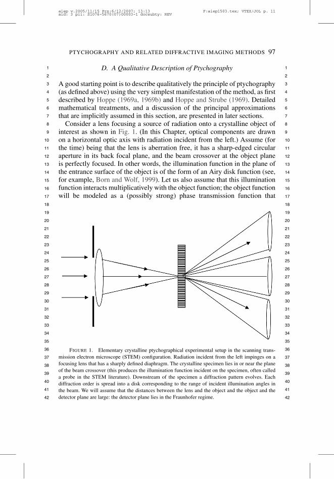
Consider a lens focusing a source of radiation onto a crystalline object ofinterest as shown in Fig. 1. (In this Chapter, optical components are drawnon a horizontal optic axis with radiation incident from the left.) Assume (forthe time) being that the lens is aberration free, it has a sharp-edged circularaperture in its back focal plane, and the beam crossover at the object planeis perfectly focused. In other words, the illumination function in the plane ofthe entrance surface of the object is of the form of an Airy disk function (see,for example, Born and Wolf, 1999). Let us also assume that this illuminationfunction interacts multiplicatively with the object function; the object functionwill be modeled as a (possibly strong) phase transmission function that
FIGURE 1. Elementary crystalline ptychographical experimental setup in the scanning trans-mission electron microscope (STEM) configuration. Radiation incident from the left impinges on afocusing lens that has a sharply defined diaphragm. The crystalline specimen lies in or near the planeof the beam crossover (this produces the illumination function incident on the specimen, often calleda probe in the STEM literature). Downstream of the specimen a diffraction pattern evolves. Eachdiffraction order is spread into a disk corresponding to the range of incident illumination angles inthe beam. We will assume that the distances between the lens and the object and the object and thedetector plane are large: the detector plane lies in the Fraunhofer regime.
aiep v.2005/11/15 Prn:6/12/2007; 13:13 F:aiep1503.tex; VTEX/JOL p. 11aid: 3 pii: S1076-5670(07)00003-1 docsubty: REV

98 RODENBURG
1 1
2 2
3 3
4 4
5 5
6 6
7 7
8 8
9 9
10 10
11 11
12 12
13 13
14 14
15 15
16 16
17 17
18 18
19 19
20 20
21 21
22 22
23 23
24 24
25 25
26 26
27 27
28 28
29 29
30 30
31 31
32 32
33 33
34 34
35 35
36 36
37 37
38 38
39 39
40 40
41 41
42 42
may also attenuate the wave as it passes through the object. Note that thetransmission function is not the same as the atomic (or optical) potentialfunction; we are not assuming the Born approximation (see Section III.C),but we are assuming that the object is quasi-2D (Cowley, 1995).
In the Fraunhofer diffraction plane, a very large distance downstream ofthe object, the far-field diffraction plane is observed. If this periodic objecthad been illuminated by a plane wave, the diffraction pattern would, as usual,consist of a series of spikes of intensity. In fact, because there is a range ofincident vectors subtending from the pupil of the lens, each diffraction peakis spread out into the shape of a disk. In the absence of a specimen, there isonly one disk – simply a shadow image projection of the aperture in the backfocal plane of the lens. When the crystalline object is in place, it is possibleto arrange for the aperture size to be such that the diffracted disks overlap oneanother as shown in Fig. 2(a). For what follows in this section, we require thatthere is a point between any two diffracted discs where only those two disksoverlap with one another (i.e., there are no multiple overlaps). If the sourceof radiation is sufficiently small and monochromatic, then illumination over
(a) (b)
(c) (d)
FIGURE 2. Schematic representation of the diffraction orders and phase relationships in theSTEM ptychograph. (a) Two diffracted disks lying in the Fraunhofer diffraction plane (the right-handside of Fig. 1). (b) Phase relationship of the underlying amplitudes of these two disks. The square rootsof the measured intensities give the lengths of the arrows, but not their phase. However, the triangleof complex numbers must be closed, although there are two indistinguishable solutions. (c) For threelinearly positioned interfering disks. (d) For 2D functions, ambiguity in this phase problem (like in allFourier phase problems) is reduced because the ratio of measurements to unknowns increases.
aiep v.2005/11/15 Prn:6/12/2007; 13:13 F:aiep1503.tex; VTEX/JOL p. 12aid: 3 pii: S1076-5670(07)00003-1 docsubty: REV
PTYCHOGRAPHY AND RELATED DIFFRACTIVE IMAGING METHODS 99
1 1
2 2
3 3
4 4
5 5
6 6
7 7
8 8
9 9
10 10
11 11
12 12
13 13
14 14
15 15
16 16
17 17
18 18
19 19
20 20
21 21
22 22
23 23
24 24
25 25
26 26
27 27
28 28
29 29
30 30
31 31
32 32
33 33
34 34
35 35
36 36
37 37
38 38
39 39
40 40
41 41
42 42
the back focal plane of the lens will be effectively coherent. In the Fraunhoferplane, this means that the diffracted beams will interfere coherently withinthese regions of overlap (provided other sources of experimental instability,such as the lens, are negligible).
In the classic diffraction phase problem (where the illumination is a planewave), the intensity (and only the intensity) of each of the diffracted beamscan be measured: the phase is lost. In Fig. 2(a), we also measure intensityonly, but now the intensity of the sum of two diffracted amplitudes alsocan be measured. Let us label these amplitudes by the complex numbers Z1and Z2, each representing the real and imaginary components (or modulus andphase) of the wave filling each disk. We can therefore measure |Z1|2, |Z2|2,and, within their region of intersection, |Z1 + Z2|2. Let the phase differencebetween Z1 and Z2 be an angle !. In the complex plane, we see a relationshipbetween amplitudes Z1 and Z2 and their sum Z1 + Z2 (shown in Fig. 2(b)).Because the moduli Z1, Z2 and Z1 +Z2 can be measured by taking the squareroot of the intensity measured in the two disks and their region of overlap,respectively, then there are only two values of ! (! and "!) that will allowthe triangle of amplitudes Z1, Z2 and Z1 +Z2 to connect with one another. Inother words, by measuring these three intensities, and assuming they interferewith one another coherently, we can derive an estimate of the phase differencebetween Z1 and Z2, but not the sense (positive or negative) of this phasedifference.
Clearly this simple experiment has greatly improved the chances of solvingthe phase problem; instead of total uncertainty in the phase of either Z1or Z2, there are now only two candidate solutions for the phase differencebetween Z1 and Z2. In fact, without loss of generality, we will always assignone of these values (say, Z1) as having an absolute phase of zero. This isbecause in any diffraction or holographic experiment only the relative phasebetween wave components can ever be possibly measured. Another way ofsaying this is that we are concerned with time-independent solutions to thewave equation, and so the absolute phase of the underlying waves (whichare time dependent) is lost and is of no significance – in the case of elasticscattering, the relative phase of the scattered wave distribution has had allthe available structural information about the object impressed upon it. If thedisk of amplitude Z1 is the straight-through (or zero order) beam, then inwhat follows we will always assign this as having zero phase: this particulartwo-beam phase problem (i.e., the relative phase of Z2) has been completelysolved apart from the ambiguity in Z2 or Z#
2 , where Z#2 is the complex
conjugate of Z2.Now consider the interference of three beams lying in a row (Fig. 2(c)).
The underlying amplitudes of these diffracted beams are labeled as Z1, Z2,and Z3. We now measure five intensities: three in the disks and two in the
aiep v.2005/11/15 Prn:6/12/2007; 13:13 F:aiep1503.tex; VTEX/JOL p. 13aid: 3 pii: S1076-5670(07)00003-1 docsubty: REV
100 RODENBURG
1 1
2 2
3 3
4 4
5 5
6 6
7 7
8 8
9 9
10 10
11 11
12 12
13 13
14 14
15 15
16 16
17 17
18 18
19 19
20 20
21 21
22 22
23 23
24 24
25 25
26 26
27 27
28 28
29 29
30 30
31 31
32 32
33 33
34 34
35 35
36 36
37 37
38 38
39 39
40 40
41 41
42 42
overlaps. These five numbers will not quite give us the six variables weneed – the modulus and phase of Z1, Z2, and Z3 – but they will give us|Z1|, |Z2|, |Z3| and two phase differences (each of which suffer from apositive/negative ambiguity). Assigning zero phase to Z1, we can solve forthe phase of all the diffracted beams (Z2 and Z3) to within four possiblesolutions, depending on the four combinations of the ambiguous phases. Itis clear that as the number, N , of diffracted beams increases, then therewill be 2N possible solutions for the one diffraction pattern. In fact, this2N ambiguity is a completely general feature of the phase problem in onedimension (Burge et al., 1976) when the object space is known to be finite(in the current case, the object and illumination function is of a particularform that gives a very clear manifestation of the phase ambiguity). Of course,if the three beams are not collinear, but form a triangle in a 2D diffractionpattern so that each beam overlaps with the other two (Fig. 2(d)), then the ratioof intensity measurements to unknowns can be increased, thereby limitingthe number of ambiguous solutions to the entire pattern. Again, even thoughwe are discussing a very specialized scattering geometry, the same argumentapplies in all diffractive imaging methods – as the dimension of the problemis increased, the likelihood of ambiguous solutions existing reduces (see forexample the discussion by Hawkes and Kasper, 1996).
The key benefit of ptychography is that a complete solution of the phase,resolving the ambiguities discussed above, can be achieved by shifting eitherthe object function or the illumination relative to one another by a smallamount, and then recording a second set of intensity measurements. We canthink of this via the Fourier shift theorem, but to begin we restrict ourselvesto a qualitative description. In the scattering geometry of Fig. 1, a shift in theillumination function can be achieved by introducing a phase ramp across theillumination pupil. One way of thinking of this is via Fig. 3(a) (which is ratherexaggerated). To produce a tilt in the wave coming out of the lens (which willconsequently lead to a shift in the illumination function at the object plane),we must rotate slightly the hemisphere of constant phase that emerges fromthe lens and which results in the wavefronts being focused at the crossover atthe object plane. If the path length is increased at the top of the hemisphereand decreased at bottom (as shown in Fig. 3(a)), then the effect is to movethe position of the illumination downward relative to the object. The pathdifference changes linearly across the hemisphere. A linear phase ramp, wherethe phase is equal to 2" times the path difference divided by the wavelength,has the equivalent influence. (In what follows, we ignore the fact that this tiltin the beam will not only shift the illumination, but also shift the diffractionpattern in the far field; in the case of most situations of interest this lattershift is negligible for typical lens working distances.) In the Fraunhofer plane,one side of the zero order (unscattered beam) has therefore been advanced in
aiep v.2005/11/15 Prn:6/12/2007; 13:13 F:aiep1503.tex; VTEX/JOL p. 14aid: 3 pii: S1076-5670(07)00003-1 docsubty: REV

PTYCHOGRAPHY AND RELATED DIFFRACTIVE IMAGING METHODS101
1 1
2 2
3 3
4 4
5 5
6 6
7 7
8 8
9 9
10 10
11 11
12 12
13 13
14 14
15 15
16 16
17 17
18 18
19 19
20 20
21 21
22 22
23 23
24 24
25 25
26 26
27 27
28 28
29 29
30 30
31 31
32 32
33 33
34 34
35 35
36 36
37 37
38 38
39 39
40 40
41 41
42 42
phase (marked as point P on Fig. 3(b)), say by a factor of ei# , and a pointnear the opposite side (P $) has been retarded in phase, say by a factor ofe"i# . If we label the underlying amplitude of the zero-order beam as Z1, thenthe complex value of the wave at P is now Z1e
i# . Suppose now that there is adiffracted beam of underlying amplitude Z2 (shown separately on the top right
(a) In the STEM configuration, a shift in the probe (indicated by the large pointer) can be achieved
by introducing a phase ramp in the plane waves (dotted lines) over the back focal plane of the lens
(incident beams illuminating the lens are drawn parallel). This is equivalent to tilting slightly the
hemisphere of wavefronts focusing the probe onto the object, consequently introducing the shift. This
manifests itself as the phase change over A(u, v).
(b) As the probe is shifted in real (object) space (top), a phase ramp is introduced over the undiffracted
beam in reciprocal space (lying in the Fraunhofer diffraction plane).
FIGURE 3.
aiep v.2005/11/15 Prn:6/12/2007; 13:13 F:aiep1503.tex; VTEX/JOL p. 15aid: 3 pii: S1076-5670(07)00003-1 docsubty: REV
102 RODENBURG
1 1
2 2
3 3
4 4
5 5
6 6
7 7
8 8
9 9
10 10
11 11
12 12
13 13
14 14
15 15
16 16
17 17
18 18
19 19
20 20
21 21
22 22
23 23
24 24
25 25
26 26
27 27
28 28
29 29
30 30
31 31
32 32
33 33
34 34
35 35
36 36
37 37
38 38
39 39
40 40
41 41
42 42
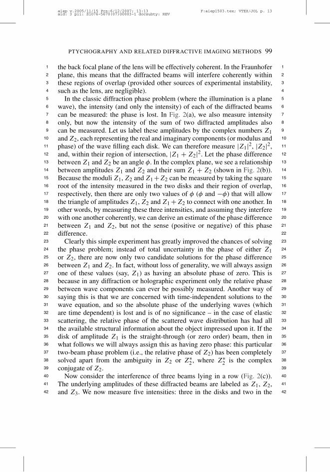
(c) At the top we draw the undiffracted beam (heavy circle) and a diffracted beam. The probe
movement has introduced phase ramps across both beams. When the spacing of the diffracted beams
is smaller (bottom circles), the equivalent points P and P $ meet up and interfere at P $$.
FIGURE 3. (continued)
of Fig. 3(b)). At an equivalent point P $ the actual complex value of the wavedisturbance is now Z2e
"i# . If these two disks overlap, then the equivalentpoints P and P $ can meet up and interfere with one another, and the totalamplitude where these points meet (P $$ in Fig. 3(c)) will be Zs , where
Zs = Z1ei# + Z2e
"i# . (1)
Before we moved the illumination by introducing these phase changes, wemeasured Z1, Z2 and Z1 + Z2. With reference to the complex sum shown inFig. 4, let Z0 be equal to Z1+Z2. In view of the complex conjugate ambiguity,Z1 + Z#
2 = Zc was also a candidate solution. However, after shifting theillumination and recording Zs , we can now discount this (wrong) solutionbecause if the same phase changes had been applied to Z1 +Z#
2 , the final sumwould have been given by Zw (see Fig. 4).
This rather naïve analysis actually summarizes the entire principle ofptychography. Later sections of the text will show that the same underlyingprinciple can be applied to extended noncrystalline objects and the illumina-tion function must not be of any particular form, as long as it is reasonablylocalized. The geometric and scattering theory approximations made in thissection will also be considered.
aiep v.2005/11/15 Prn:6/12/2007; 13:13 F:aiep1503.tex; VTEX/JOL p. 16aid: 3 pii: S1076-5670(07)00003-1 docsubty: REV

PTYCHOGRAPHY AND RELATED DIFFRACTIVE IMAGING METHODS103
1 1
2 2
3 3
4 4
5 5
6 6
7 7
8 8
9 9
10 10
11 11
12 12
13 13
14 14
15 15
16 16
17 17
18 18
19 19
20 20
21 21
22 22
23 23
24 24
25 25
26 26
27 27
28 28
29 29
30 30
31 31
32 32
33 33
34 34
35 35
36 36
37 37
38 38
39 39
40 40
41 41
42 42
FIGURE 4. How ptychography unlocks the complex conjugate phase ambiguity. In this dia-gram, the lengths of filled pointers represent the square root of the intensity of our four measurements(two from the centers of the diffracted disks, two from the overlap region at different probe positions).Before moving the illumination (probe) the three initial measurements (top left) have two possiblesolutions (top and middle right). When the phase shifts (Fig. 3) are applied (bottom left), the wrong("!) phase can be discounted: the hatched pointer (Zw) is not the length of the measured modulus Zs .All phases are plotted with respect to Z1; in practice, Z1 and Z2 rotate equal angles in oppositedirections, but the effect on the measured moduli is the same.
E. Mathematical Formulation of Crystalline STEM Ptychography
For the sake of simplicity, this section adopts an image processing-type ofnomenclature and not an optical or electron scattering nomenclature. Sec-tion III will connect the relevant wave k-vectors with the implicit geometricapproximations made here. This section simply defines a mathematical form
aiep v.2005/11/15 Prn:6/12/2007; 13:13 F:aiep1503.tex; VTEX/JOL p. 17aid: 3 pii: S1076-5670(07)00003-1 docsubty: REV

104 RODENBURG
1 1
2 2
3 3
4 4
5 5
6 6
7 7
8 8
9 9
10 10
11 11
12 12
13 13
14 14
15 15
16 16
17 17
18 18
19 19
20 20
21 21
22 22
23 23
24 24
25 25
26 26
27 27
28 28
29 29
30 30
31 31
32 32
33 33
34 34
35 35
36 36
37 37
38 38
39 39
40 40
41 41
42 42
of the 2D Fourier transform as
%f (x, y) =!!
f (x, y)ei2"(ux+vy) dx dy = F(u, v), (2a)
and its inverse as
%"1F(u, v) =!!
F(u, v)e"i2"(ux+vy) dx dy = f (x, y), (2b)
where f (x, y) is a 2D image or transmission function that may be complexvalued, described by Cartesian coordinates x and y; F(u, v) is the Fouriertransform of f (x, y); u and v are coordinates in reciprocal space (that is, theFourier transform space); and for the compactness of later equations we usethe symbol % to represent the whole Fourier integral. This definition of theFourier transform differs from that used in some fields (including electronmicroscopy, although not crystallography) by having a positive exponential.The inclusion of the factor of 2" in the exponential renders the definitionof the inverse much simpler by not requiring a scaling factor dependent onthe dimensionality of the functions involved. This greatly simplifies somearithmetic manipulations that must be used in later sections.
As before, let us assume that the object can be represented by a thincomplex transmission function. In other words, the presence of the object hasthe effect of changing the phase and intensity (or, rather, modulus) of the waveincident upon it. The exit wave, $e(x, y), immediately behind the object, willhave the form
$e(x, y) = a(x, y) · q(x, y), (3)
where x and y are coordinates lying in the plane of the (2D) object function,a(x, y) is the complex illumination function falling on the object, and q(x, y)is the complex transmission function of the object. As emphasized previously,q(x, y) is not the potential or optical potential of the object; it is equal tothe exit wave that would emerge from a thin (but possibly very stronglyscattering) object when illuminated with a monochromatic plane wave. Fora thick specimen, we might hope that
q(x, y) = ei"
%V (x,y,z) dz, (4)
where V (x, y, z) is the optical potential (or, in the case of high electrons,the atomic potential) of the object, and % is a constant describing thestrength of the scattering for the particular radiation involved. In this case theptychographical image derived below can be related directly to the projectionof the potential (by taking the logarithm of q(x, y) – at least in the absenceof phase wrapping), despite strong (dynamical) scattering. In fact, this is notthe case for thick specimens because the integral with respect to z does not
aiep v.2005/11/15 Prn:6/12/2007; 13:13 F:aiep1503.tex; VTEX/JOL p. 18aid: 3 pii: S1076-5670(07)00003-1 docsubty: REV
PTYCHOGRAPHY AND RELATED DIFFRACTIVE IMAGING METHODS105
1 1
2 2
3 3
4 4
5 5
6 6
7 7
8 8
9 9
10 10
11 11
12 12
13 13
14 14
15 15
16 16
17 17
18 18
19 19
20 20
21 21
22 22
23 23
24 24
25 25
26 26
27 27
28 28
29 29
30 30
31 31
32 32
33 33
34 34
35 35
36 36
37 37
38 38
39 39
40 40
41 41
42 42
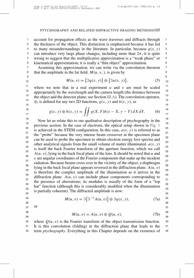
account for propagation effects as the wave traverses and diffracts throughthe thickness of the object. This distinction is emphasized because it has ledto many misunderstandings in the literature. In particular, because q(x, y)can introduce very large phase changes, including more than 2" , it is quitewrong to suggest that the multiplicative approximation is a “weak phase” orkinematical approximation; it is really a “thin object” approximation.
Assuming this approximation, we can write via the convolution theoremthat the amplitude in the far field, M(u, v, ), is given by
M(u, v) =#%q(x, y)
$&
#%a(x, y)
$, (5)
where we note that in a real experiment u and v are must be scaledappropriately by the wavelength and the camera length (the distance betweenthe object and the detector plane; see Section III.A). The convolution operator,&, is defined for any two 2D functions, g(x, y) and h(x, y), as
g(x, y) & h(x, y) =!!
g(X, Y )h(x " X, y " Y ) dX dY. (6)
Now let us relate this to our qualitative description of ptychography in theprevious section. In the case of electrons, the optical setup shown in Fig. 1is achieved in the STEM configuration. In this case, a(x, y) is referred to asthe “probe” because the very intense beam crossover at the specimen planecan be used to probe the specimen to obtain electron energy loss spectra andother analytical signals from the small volume of matter illuminated. a(x, y)is itself the back Fourier transform of the aperture function, which we callA(u, v), lying in the back focal plane of the lens. It should be noted that u andv are angular coordinates of the Fourier components that make up the incidentradiation. Because beams cross over in the vicinity of the object, a diaphragmlying in the back focal plane appears reversed in the diffraction plane. A(u, v)is therefore the complex amplitude of the illumination as it arrives in thediffraction plane. A(u, v) can include phase components corresponding tothe presence of aberrations; its modulus is usually of the form of a “tophat” function (although this is considerably modified when the illuminationis partially coherent). The diffracted amplitude is now:
M(u, v) = %%%"1A(u, v)
&& %q(x, y), (7a)
or
M(u, v) = A(u, v) & Q(u, v), (7b)
where Q(u, v) is the Fourier transform of the object transmission function.It is this convolution (folding) in the diffraction plane that leads to theterm ptychography. Everything in this Chapter depends on the existence of
aiep v.2005/11/15 Prn:6/12/2007; 13:13 F:aiep1503.tex; VTEX/JOL p. 19aid: 3 pii: S1076-5670(07)00003-1 docsubty: REV

106 RODENBURG
1 1
2 2
3 3
4 4
5 5
6 6
7 7
8 8
9 9
10 10
11 11
12 12
13 13
14 14
15 15
16 16
17 17
18 18
19 19
20 20
21 21
22 22
23 23
24 24
25 25
26 26
27 27
28 28
29 29
30 30
31 31
32 32
33 33
34 34
35 35
36 36
37 37
38 38
39 39
40 40
41 41
42 42
this convolution. The STEM configuration is particularly straightforward tounderstand when we assume a very simple form of A(u, v) – a sharply definedcircular aperture. In our simplest manifestation of ptychography, we make twomeasurements, intensities I1(u, v) and I2(u, v), each from different positionsof the probe, where
I1(u, v) =''A(u, v) & Q(u, v)
''2 (8a)
and
I2(u, v) =''%A(u, v)eiu&x
&& Q(u, v)
''2 (8b)
and where we have assumed the second measurement is made with theillumination function shifted with respect to the origin in real space by adistance &x in the x-direction to give a(x " &x, y): The exponential derivesfrom the Fourier shift theorem, namely, that
%g(x + &x) =!
g(x + &x)ei2"ux dx =!
g(X)ei2"u(X"&x) dX
= G(u)e"iu2"&x (9)
for any function g(x) whose Fourier transform is G(u). In the simplest versionof ptychography, we are interested in the case of q(x, y) being a periodic 2Dcrystal. Q(u, v) then only has values on an equivalent 2D reciprocal lattice.Let us suppose for simplicity that this lattice is rectilinear with a periodicityof &u and &v, in the u and v directions, respectively. We can say that
Q(u, v) =(
n,m
Qn,m'(u " n&u, v " m&v), (10)
where Qm,n is a complex number associated with the amplitude of a recipro-cal lattice point indexed by m and n, the sum is over the positive and negativeintegers for all m and n, and '(u, v) is a Dirac delta function defined as
'(u " u0, v " v0) =)
0 for u '= u0 or v '= v0,
( for u = u0 and v = v0(11a)
and where(!
"('(u " u0, v " v0) du dv = 1. (11b)
To achieve the overlapping disks we described in the previous section(Fig. 2(a)), the aperture function A(u, v) must have a diameter of at least&v or &u, whichever is the larger. Suppose that &u > ( > &u/2, where ( isradius of the aperture, as shown in Fig. 5. As before, we consider just two of
aiep v.2005/11/15 Prn:6/12/2007; 13:13 F:aiep1503.tex; VTEX/JOL p. 20aid: 3 pii: S1076-5670(07)00003-1 docsubty: REV

PTYCHOGRAPHY AND RELATED DIFFRACTIVE IMAGING METHODS107
1 1
2 2
3 3
4 4
5 5
6 6
7 7
8 8
9 9
10 10
11 11
12 12
13 13
14 14
15 15
16 16
17 17
18 18
19 19
20 20
21 21
22 22
23 23
24 24
25 25
26 26
27 27
28 28
29 29
30 30
31 31
32 32
33 33
34 34
35 35
36 36
37 37
38 38
39 39
40 40
41 41
42 42
FIGURE 5. In the simplest STEM implementation of crystalline ptychography, intensity ismeasured at the centers of the zero-order and first-order diffraction disks and at the midpoint of theiroverlap region.
the disks in the far field: the zero-order beam (n = m = 0) and one diffractedbeam (n = 1, m = 0), then
Q(u, v) = Q0,0'(u, v) + Q1,0'(u " &u) (12)
and so
M(u, v) = Q0,0A(u, v) + Q1,0A(u " &u, v). (13)
With reference to Fig. 5, let us measure the intensity at a point midwaybetween the centers of the two interfering aperture functions, namely, at u =&u/2 and v = 0. The wave amplitude at this point is
M
*&u
2, 0
+= Q0,0A
*&u
2, 0
++ Q1,0A
*"&u
2, 0
+(14)
and hence the intensity at this point in the diffraction plane with the illumina-tion field (the probe) on axis, is
I1
*&u
2, 0
+=
''''Q0,0A
*&u
2, 0
++ Q1,0A
*"&u
2, 0
+''''2
. (15)
We now move the probe a distance &x in the x-direction (parallel withthe reciprocal coordinate u). From Eq. (8b) we obtain a second intensitymeasurement
I2
*&u
2, 0
+=
''''Q0,0A
*(
2, 0
+ei &2"u
2 &x + Q1,0A
*"(
2, 0
+e"i &2"u
2 &x
''''2
.
(16)
aiep v.2005/11/15 Prn:6/12/2007; 13:13 F:aiep1503.tex; VTEX/JOL p. 21aid: 3 pii: S1076-5670(07)00003-1 docsubty: REV

108 RODENBURG
1 1
2 2
3 3
4 4
5 5
6 6
7 7
8 8
9 9
10 10
11 11
12 12
13 13
14 14
15 15
16 16
17 17
18 18
19 19
20 20
21 21
22 22
23 23
24 24
25 25
26 26
27 27
28 28
29 29
30 30
31 31
32 32
33 33
34 34
35 35
36 36
37 37
38 38
39 39
40 40
41 41
42 42
The amplitudes of these two equations are identical in form to the qualitativedescription derived in Section II.E [Eq. (1)], with the phase term # replacedby "&u&x and with Z1 and Z2 replaced by the underlying phases ofthe lattice reflections Q0,0 and Q1,0. In the previous section we assumedthat the aperture function A(u, v) did not have any aberrations (i.e., phasecomponents) across it; this means the value of A(u, v) is unity, and so thisterm does not appear in Eq. (1). In general, the aperture function will havephase changes across it, corresponding to defocus, spherical aberration, andso on, and so these must be accounted for in some way – indeed the probemovement (which leads to a linear phase ramp multiplying the aperturefunction, as in Eq. (8b) is itself a sort of aberration term.
It should be pointed out that in general it may not be experimentallyconvenient to use an aperture function that is small enough to guarantee thatthere exist points in the diffraction pattern where only two adjacent diffracteddisks overlap. Clearly, as the unit cell increases in size, the diffraction disksbecome more and more closely spaced in the diffraction plane. In the limitof a nonperiodic object, it may appear as if the ptychographical principle isno longer applicable, because the pairs of interfering beams can no longer becleanly separated. In fact, we will see in Section IV that this is not the case,provided we adopt more elaborate processing strategies.
In this very simplest arrangement with just two diffracted beams, we stillneed to measure a total of four intensities to derive their relative phase. Aswell as measurements made at the disk overlaps, we need the intensities of thediffracted beams themselves (lying outside the region of overlap, but within asingle disk, as in Fig. 5). Our task is to solve for the phase difference betweenQ0,0 and Q1,0 given that
|Q0,0|2 = I1(0, 0) = I2(0, 0),
|Q1,0|2 = I1(&u, 0) = I2(0, 0),(17)
|Q0,0 + Q1,0|2 = I1
*&u
2, 0
+,
''Q0,0ei# + Q1,0e
"i#''2 = I2
*&u
2, 0
+.
Conventional crystallography is usually interested only in the structure ofthe object, not its absolute position in terms of x and y. A displacementambiguity always occurs in the classic PDI phase problem: the intensity of theFraunhofer plane is unaffected by lateral displacements of the object. In otherwords, normal diffraction is never sensitive to a linear-phase ramp appliedacross the diffraction plane. The usual crystallographic convention assumesthat a point of symmetry is implicitly at the origin of real space. In contrast, inptychography there is an explicit definition of absolute position in real space –
aiep v.2005/11/15 Prn:6/12/2007; 13:13 F:aiep1503.tex; VTEX/JOL p. 22aid: 3 pii: S1076-5670(07)00003-1 docsubty: REV

PTYCHOGRAPHY AND RELATED DIFFRACTIVE IMAGING METHODS109
1 1
2 2
3 3
4 4
5 5
6 6
7 7
8 8
9 9
10 10
11 11
12 12
13 13
14 14
15 15
16 16
17 17
18 18
19 19
20 20
21 21
22 22
23 23
24 24
25 25
26 26
27 27
28 28
29 29
30 30
31 31
32 32
33 33
34 34
35 35
36 36
37 37
38 38
39 39
40 40
41 41
42 42
the known position of the confined illumination – but there is no reason tosuppose that the crystal itself just happens to be aligned centrosymmetricallywith this point in space. If the crystallographic phase of Q(u, v) (arising fromadopting a centrosymmetric convention for the phase of the diffracted beams)is Q0(u, v), then
Q(u, v) = Q0(u, v)"i(u&x+v&y), (18)
where &x and &y is the displacement of the crystal relative to the optic axis.As a result, the particular phases of Q0,0 and Q1,0 that are consistent withEq. (17) relate to exact geometry of the lens, which defines the exact positionof the illumination function a(x, y). In practice, the value of # , proportional tothe probe movement distance, can be chosen at will. In almost all conceivableexperimental implementations of crystalline STEM (electron) ptychography,the exact position of the probe relative to the object is not known accurately;only relative displacements can be measured (say by applying an offset to theprobe scan coils in STEM). In this case, we could choose to scan the probeposition until I1(
&v2 , 0) is at a maximum and simply assert the convention
that the probe at this position is at x = y = 0. Relative to this definition,then Q0,0 and Q1,0 have zero phase difference between them (because in thiscondition they add to give maximum modulus). However, the phase of allother reflections will be altered accordingly via Eq. (18).
Equation (17) can be solved either geometrically (via the complex planeconstruction in Fig. 2(b)) or by direct substitution. Ill-defined solutions canstill arise if we choose the value of # unfavorably; for example, we find thatI1 = I2 if either &x = n"/&u, where n is integer, or when # /2 happens to bethe same as the phase difference between Q0,0 and Q1,0. We note, however,that Eq. (17) only represents a tiny fraction of the number of measurementsat our disposal. Obviously, the intensity at the midpoints of all pairs ofreflections must be tracked to solve for all of the relative phases of all pairsof adjacent beams. Many diffraction patterns, from many probe positions,can also be recorded instead of just the two required to unlock the complexconjugate ambiguity. Achieving this in the most computationally favorableway has been the subject of much work and is discussed in Section IV.
F. Illumination of a “Top Hat” or Objects with Finite Support
The crystalline STEM implementation of ptychography is easy to understandintuitively because the illumination function (probe) in real space is of aparticular form that conveniently provides a far-field diffraction pattern inwhich the interferences of the various pairs of beams are tidily separated.In general, the illumination function can be of any functional form. In the
aiep v.2005/11/15 Prn:6/12/2007; 13:13 F:aiep1503.tex; VTEX/JOL p. 23aid: 3 pii: S1076-5670(07)00003-1 docsubty: REV
110 RODENBURG
1 1
2 2
3 3
4 4
5 5
6 6
7 7
8 8
9 9
10 10
11 11
12 12
13 13
14 14
15 15
16 16
17 17
18 18
19 19
20 20
21 21
22 22
23 23
24 24
25 25
26 26
27 27
28 28
29 29
30 30
31 31
32 32
33 33
34 34
35 35
36 36
37 37
38 38
39 39
40 40
41 41
42 42
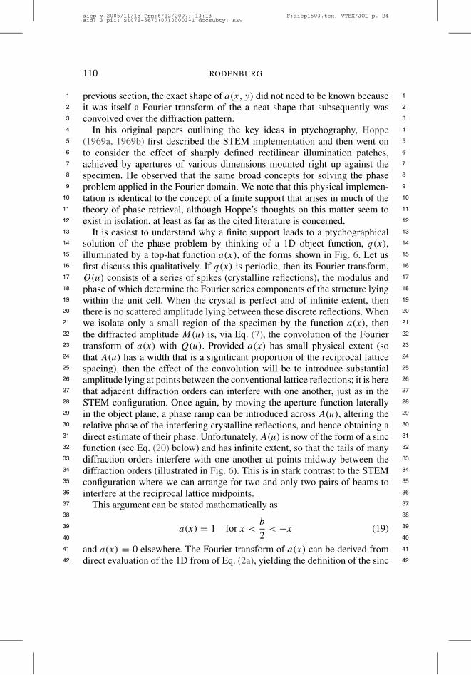
previous section, the exact shape of a(x, y) did not need to be known becauseit was itself a Fourier transform of the a neat shape that subsequently wasconvolved over the diffraction pattern.
In his original papers outlining the key ideas in ptychography, Hoppe(1969a, 1969b) first described the STEM implementation and then went onto consider the effect of sharply defined rectilinear illumination patches,achieved by apertures of various dimensions mounted right up against thespecimen. He observed that the same broad concepts for solving the phaseproblem applied in the Fourier domain. We note that this physical implemen-tation is identical to the concept of a finite support that arises in much of thetheory of phase retrieval, although Hoppe’s thoughts on this matter seem toexist in isolation, at least as far as the cited literature is concerned.
It is easiest to understand why a finite support leads to a ptychographicalsolution of the phase problem by thinking of a 1D object function, q(x),illuminated by a top-hat function a(x), of the forms shown in Fig. 6. Let usfirst discuss this qualitatively. If q(x) is periodic, then its Fourier transform,Q(u) consists of a series of spikes (crystalline reflections), the modulus andphase of which determine the Fourier series components of the structure lyingwithin the unit cell. When the crystal is perfect and of infinite extent, thenthere is no scattered amplitude lying between these discrete reflections. Whenwe isolate only a small region of the specimen by the function a(x), thenthe diffracted amplitude M(u) is, via Eq. (7), the convolution of the Fouriertransform of a(x) with Q(u). Provided a(x) has small physical extent (sothat A(u) has a width that is a significant proportion of the reciprocal latticespacing), then the effect of the convolution will be to introduce substantialamplitude lying at points between the conventional lattice reflections; it is herethat adjacent diffraction orders can interfere with one another, just as in theSTEM configuration. Once again, by moving the aperture function laterallyin the object plane, a phase ramp can be introduced across A(u), altering therelative phase of the interfering crystalline reflections, and hence obtaining adirect estimate of their phase. Unfortunately, A(u) is now of the form of a sincfunction (see Eq. (20) below) and has infinite extent, so that the tails of manydiffraction orders interfere with one another at points midway between thediffraction orders (illustrated in Fig. 6). This is in stark contrast to the STEMconfiguration where we can arrange for two and only two pairs of beams tointerfere at the reciprocal lattice midpoints.
This argument can be stated mathematically as
a(x) = 1 for x <b
2< "x (19)
and a(x) = 0 elsewhere. The Fourier transform of a(x) can be derived fromdirect evaluation of the 1D from of Eq. (2a), yielding the definition of the sinc
aiep v.2005/11/15 Prn:6/12/2007; 13:13 F:aiep1503.tex; VTEX/JOL p. 24aid: 3 pii: S1076-5670(07)00003-1 docsubty: REV

PTYCHOGRAPHY AND RELATED DIFFRACTIVE IMAGING METHODS111
1 1
2 2
3 3
4 4
5 5
6 6
7 7
8 8
9 9
10 10
11 11
12 12
13 13
14 14
15 15
16 16
17 17
18 18
19 19
20 20
21 21
22 22
23 23
24 24
25 25
26 26
27 27
28 28
29 29
30 30
31 31
32 32
33 33
34 34
35 35
36 36
37 37
38 38
39 39
40 40
41 41
42 42
FIGURE 6. Illustrating ptychographical interference when the illumination function is of theform of a top hat (or there exists, equivalently, a support function). We assume the multiplicativeapproximation in real space (top), giving rise to an exit wave consisting of just two spikes ofamplitude. In reciprocal space, we form the convolution, adding together a row of sinc functions.Rather than measuring points halfway between the reciprocal lattice points, the points where we inferthat the amplitude of adjacent reflected moduli are equal (bottom diagram) give the most accurateptychographic phase. In fact, this particular rather unrealistic example (a series of delta functions inthe real and reciprocal space of q(x)) raises an interesting paradox. We know that, as a function ofthe position of the illumination, the resulting Young’s slit intensity has either zero or unity intensityat the exact halfway point between the diffraction reflections (depending on the width of the top hat).This is because of the way the small ringing effects in phase-altered sinc functions add. When the unitcell has structure, and the top hat is the same size as the unit cell, we can infer the ptychographicalphases, but the ringing effects will still corrupt the estimate (unlike in the STEM configuration wherethe interference terms are neatly separated).
function, such that
%a(x) = A(u) = bsin "ub
"ub= b sinc("ub). (20)
If the object of function is crystalline, it consists of a series of deltafunctions convolved with the structure of the unit cell that can be written as
q(x) =*(
n
'(x " n&x)
+& fc(x). (21)
aiep v.2005/11/15 Prn:6/12/2007; 13:13 F:aiep1503.tex; VTEX/JOL p. 25aid: 3 pii: S1076-5670(07)00003-1 docsubty: REV

112 RODENBURG
1 1
2 2
3 3
4 4
5 5
6 6
7 7
8 8
9 9
10 10
11 11
12 12
13 13
14 14
15 15
16 16
17 17
18 18
19 19
20 20
21 21
22 22
23 23
24 24
25 25
26 26
27 27
28 28
29 29
30 30
31 31
32 32
33 33
34 34
35 35
36 36
37 37
38 38
39 39
40 40
41 41
42 42
The amplitude in the far field is
M(u) = %%a(x) · q(x)
&= A(x) & Q(u). (22)
Now the Fourier transform of a periodic array of delta functions of separation&x is itself an array of delta functions of separation &u = 1/&x. Hence
Q(u) =*(
n
'(u " n&u)
+·,%fc(x)
-. (23)
In analogy with Eq. (10), this can be written as
Q(u, v) =(
n
Qn'(u " n&u), (24)
with the understanding that the Qn are the Fourier coefficients (or structurefactors) of the unit cell fc(x). Therefore
M(u) =(
n
Qn'(u " n&u) & b sinc("ub). (25)
This convolution can be pictured as simply the addition of a series of sincfunctions, each centered on a diffraction pattern reflection and multiplied bythe modulus and phase of that reflection (Fig. 6); sinc("ub) passes throughzero whenever ub is a non-zero integer. So when b = 1/&u = &x, a sincfunction centered on a particular reflection passes through zero at all otherreflections. In other words, when the object plane aperture is the same widthas the unit cell, the intensity measured at points in the diffraction patternwhere the normal diffraction peaks would occur is unaffected by the presenceof the aperture (except for a constant scaling factor). But in addition tothese conventional diffraction data, the interference intensities between theconventional diffraction orders can be measured. Hoppe (1969a) suggestedexamining points illustrated at the bottom of Fig. 6 where, given the knownmoduli of the adjacent diffraction orders, one could infer the point at whichthe associated sinc functions would have equal moduli. The actual modulus(square root of intensity) measured at this exact point would be indicativeof the phase difference between the two adjacent reflections, give or takethe usual complex conjugate ambiguity (see Fig. 4), which, as before, canbe resolved by shifting a(x) by less than the width of the unit cell. Unlikewith the STEM, we now have the problem that all other diffracted reflectionswill also add amplitude to points lying between any pair of reflections. Infact, these additions in the artificial example shown in Fig. 6 lead to a strangeparadox (see caption). Nevertheless, Hoppe and Strube (1969) demonstratedin an optical experiment that in general the phase differences of adjacentdiffraction orders could indeed be measured with reasonable accuracy usingthis method.
aiep v.2005/11/15 Prn:6/12/2007; 13:13 F:aiep1503.tex; VTEX/JOL p. 26aid: 3 pii: S1076-5670(07)00003-1 docsubty: REV

PTYCHOGRAPHY AND RELATED DIFFRACTIVE IMAGING METHODS113
1 1
2 2
3 3
4 4
5 5
6 6
7 7
8 8
9 9
10 10
11 11
12 12
13 13
14 14
15 15
16 16
17 17
18 18
19 19
20 20
21 21
22 22
23 23
24 24
25 25
26 26
27 27
28 28
29 29
30 30
31 31
32 32
33 33
34 34
35 35
36 36
37 37
38 38
39 39
40 40
41 41
42 42
This process of interfering adjacent diffracted reflections is another wayof thinking about where both the source of the phase information and theambiguous solutions arise in conventional PDI. If we assume the object is infact periodic (and in this discussion, one-dimensional), with a periodicity ofits entire width, then the aperture function (support) is also the size of theunit cell. In reciprocal space, the crystalline lattice points must be convolutedwith sinc functions, each one of which has zero value at all reflections exceptthe one on which it is centered. This hypothetical aperture does not alter therelative intensity of the diffracted orders, but it does mean the diffracted ordersinterfere with one another at the “in-between” reciprocal lattice points. Hence,we have the classic phase problem with the 2N complex conjugate ambiguity.
G. Two-Beam Ptychography
In referring back to the STEM implementation of ptychography, we note thata large part of the illumination disk is irrelevant as far as the phase determina-tion process is concerned. In fact, all that is need are two pinholes, separatedin the back focal plane of the lens by the exact distance between the latticepoints. This is equivalent to illuminating the object by two coherent planewaves, inclined to one another by twice the Bragg angle (this method relatesvery closely to the Bragg–Brentano data set, discussed in Section IV.B). At theobject, the waves interfere and give rise to a sinusoidal interference pattern ofthe same periodicity as that of the unit cell. In the far field we now have thecoherent summation of two diffraction patterns, offset from one another byone reciprocal lattice vector. The amplitude of each of the reflections in theresulting pattern is what would have been obtained within the overlap regionof each pair of disks in the STEM configuration. Once again, the complex-conjugate ambiguity can be resolved by introducing a shift in the illuminationpattern of radiation which, as before, can be effected by introducing a changein phase in either or both the incident beams.
The article by Hegerl and Hoppe (1972) uses this condition to evaluate theptychographical phase differences between reflections in a model calculation.In this manifestation of ptychography, the illumination function must be bya beam splitter or diffraction grating (as in the work of Berndt and Doll,1976, 1978, 1983) and is therefore much harder to implement experimentallythan the STEM configuration. However, it does have the distinct advantagethat a crystalline object function can be very large, consisting of manythousands of unit cells, all of which are bathed in the illuminating beam. Thisis because there is no confined probe: the two incident plane waves extendover the entire object. In the far field, all the relevant intensity is channeledinto exactly (and only) those points that give rise to the ptychographical
aiep v.2005/11/15 Prn:6/12/2007; 13:13 F:aiep1503.tex; VTEX/JOL p. 27aid: 3 pii: S1076-5670(07)00003-1 docsubty: REV
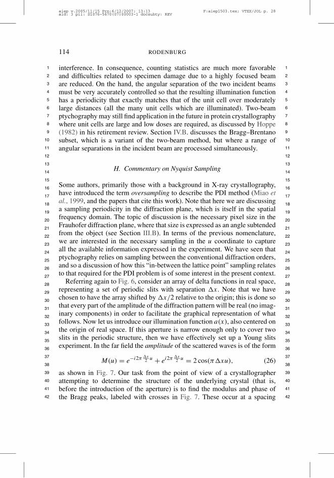
114 RODENBURG
1 1
2 2
3 3
4 4
5 5
6 6
7 7
8 8
9 9
10 10
11 11
12 12
13 13
14 14
15 15
16 16
17 17
18 18
19 19
20 20
21 21
22 22
23 23
24 24
25 25
26 26
27 27
28 28
29 29
30 30
31 31
32 32
33 33
34 34
35 35
36 36
37 37
38 38
39 39
40 40
41 41
42 42
interference. In consequence, counting statistics are much more favorableand difficulties related to specimen damage due to a highly focused beamare reduced. On the hand, the angular separation of the two incident beamsmust be very accurately controlled so that the resulting illumination functionhas a periodicity that exactly matches that of the unit cell over moderatelylarge distances (all the many unit cells which are illuminated). Two-beamptychography may still find application in the future in protein crystallographywhere unit cells are large and low doses are required, as discussed by Hoppe(1982) in his retirement review. Section IV.B. discusses the Bragg–Brentanosubset, which is a variant of the two-beam method, but where a range ofangular separations in the incident beam are processed simultaneously.
H. Commentary on Nyquist Sampling
Some authors, primarily those with a background in X-ray crystallography,have introduced the term oversampling to describe the PDI method (Miao etal., 1999, and the papers that cite this work). Note that here we are discussinga sampling periodicity in the diffraction plane, which is itself in the spatialfrequency domain. The topic of discussion is the necessary pixel size in theFrauhofer diffraction plane, where that size is expressed as an angle subtendedfrom the object (see Section III.B). In terms of the previous nomenclature,we are interested in the necessary sampling in the u coordinate to captureall the available information expressed in the experiment. We have seen thatptychography relies on sampling between the conventional diffraction orders,and so a discussion of how this “in-between the lattice point” sampling relatesto that required for the PDI problem is of some interest in the present context.
Referring again to Fig. 6, consider an array of delta functions in real space,representing a set of periodic slits with separation &x. Note that we havechosen to have the array shifted by &x/2 relative to the origin; this is done sothat every part of the amplitude of the diffraction pattern will be real (no imag-inary components) in order to facilitate the graphical representation of whatfollows. Now let us introduce our illumination function a(x), also centered onthe origin of real space. If this aperture is narrow enough only to cover twoslits in the periodic structure, then we have effectively set up a Young slitsexperiment. In the far field the amplitude of the scattered waves is of the form
M(u) = e"i2" &x2 u + ei2" &x
2 u = 2 cos("&xu), (26)
as shown in Fig. 7. Our task from the point of view of a crystallographerattempting to determine the structure of the underlying crystal (that is,before the introduction of the aperture) is to find the modulus and phase ofthe Bragg peaks, labeled with crosses in Fig. 7. These occur at a spacing
aiep v.2005/11/15 Prn:6/12/2007; 13:13 F:aiep1503.tex; VTEX/JOL p. 28aid: 3 pii: S1076-5670(07)00003-1 docsubty: REV
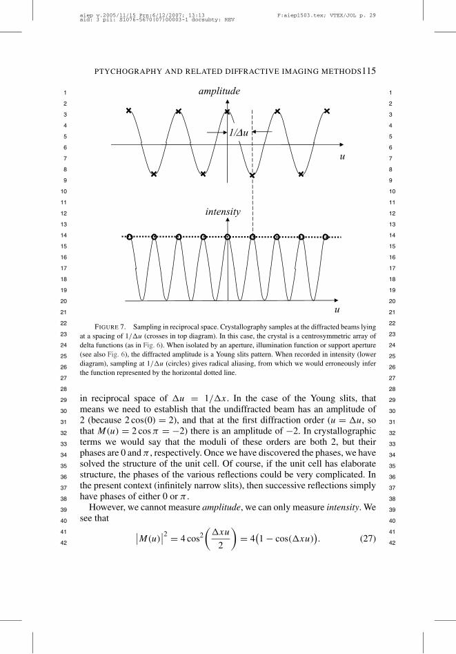
PTYCHOGRAPHY AND RELATED DIFFRACTIVE IMAGING METHODS115
1 1
2 2
3 3
4 4
5 5
6 6
7 7
8 8
9 9
10 10
11 11
12 12
13 13
14 14
15 15
16 16
17 17
18 18
19 19
20 20
21 21
22 22
23 23
24 24
25 25
26 26
27 27
28 28
29 29
30 30
31 31
32 32
33 33
34 34
35 35
36 36
37 37
38 38
39 39
40 40
41 41
42 42
FIGURE 7. Sampling in reciprocal space. Crystallography samples at the diffracted beams lyingat a spacing of 1/&u (crosses in top diagram). In this case, the crystal is a centrosymmetric array ofdelta functions (as in Fig. 6). When isolated by an aperture, illumination function or support aperture(see also Fig. 6), the diffracted amplitude is a Young slits pattern. When recorded in intensity (lowerdiagram), sampling at 1/&u (circles) gives radical aliasing, from which we would erroneously inferthe function represented by the horizontal dotted line.
in reciprocal space of &u = 1/&x. In the case of the Young slits, thatmeans we need to establish that the undiffracted beam has an amplitude of2 (because 2 cos(0) = 2), and that at the first diffraction order (u = &u, sothat M(u) = 2 cos " = "2) there is an amplitude of "2. In crystallographicterms we would say that the moduli of these orders are both 2, but theirphases are 0 and " , respectively. Once we have discovered the phases, we havesolved the structure of the unit cell. Of course, if the unit cell has elaboratestructure, the phases of the various reflections could be very complicated. Inthe present context (infinitely narrow slits), then successive reflections simplyhave phases of either 0 or " .
However, we cannot measure amplitude, we can only measure intensity. Wesee that
''M(u)''2 = 4 cos2
*&xu
2
+= 4
,1 " cos(&xu)
-. (27)
aiep v.2005/11/15 Prn:6/12/2007; 13:13 F:aiep1503.tex; VTEX/JOL p. 29aid: 3 pii: S1076-5670(07)00003-1 docsubty: REV

116 RODENBURG
1 1
2 2
3 3
4 4
5 5
6 6
7 7
8 8
9 9
10 10
11 11
12 12
13 13
14 14
15 15
16 16
17 17
18 18
19 19
20 20
21 21
22 22
23 23
24 24
25 25
26 26
27 27
28 28
29 29
30 30
31 31
32 32
33 33
34 34
35 35
36 36
37 37
38 38
39 39
40 40
41 41
42 42
In other words, the periodicity of the diffracted intensity is now exactlythe same as the periodicity of the reciprocal lattice, as shown in the lowerhalf of Fig. 7. This is as would be expected. After all, if we were to slowlyincrease the width of the aperture, and hence let more and more pairs of realspace delta functions contribute to the scattered amplitude, then the intensitywould concentrate itself only at the reciprocal lattice points. However, froma signal-processing point of view, sampling intensity only at the reciprocallattice points undersamples the data by a factor of 2. In the simplest case of theYoung’s slits, if we only sample at the peaks of the intensity (shown as circlesin Fig. 7), then from a computerized representation of the data we wouldconclude that the diffraction pattern has a numerical value of intensity of 4 atall points in the diffraction plane. In contrast, the Nyquist condition requiresa function to be sampled at twice the frequency of the highest frequencycomponent contributing to that function. In the case of intensity (as opposedto amplitude) the Nyquist sampling is &u/2, not &u.
This point is belabored here because I believe that the use of termsdouble sampling or oversampling in reference to diffracted intensity is aserious misnomer. The appropriate Nyquist sampling of the intensity of anydiffraction pattern is incontrovertibly &u/2. Of course, crystallographersonly ever need to concern themselves the measurable intensity at the actualreciprocal lattice points. But from an information point of view, ignoring thegaps between diffraction orders introduces a massive quantity of a prioriinformation: that for a perfect crystal all pixels lying between diffractionorders have zero intensity. Sayre’s short paper in 1952 (Sayre, 1952) un-derlined this point, yet many workers in the field of PDI still refer to theneed for oversampling (in the Nyquist sense) the diffraction intensity – a usethat has sadly become widespread. Sampling intensity at half the reciprocallattice periodicity exactly satisfies the Nyquist condition. On the contrary,conventional crystallography undersamples the diffracted intensity by a factorof 2: it can legitimately do this by assuming a priori that, for an infinite crystal,there is no intensity lying between the diffraction spots.
All noncrystallographic discussions of the phase problem infer this factfrom the point of view of the width of the autocorrelation function or viasimple consideration of the frequency-doubling effect of intensity relativeto amplitude. It would seem, however, that Hoppe was the first author toexplicitly state a direct method for the solution for the missing N phasesfrom N diffraction orders via the 2N numbers associated with the Nyquistfrequency of intensity. In fact, he suggested that the ideal point to samplethe intensity between the diffracted orders was at those points where thetwo adjacent sinc functions (arising from the ptychographical convolution)have identical modulus, as inferred from the form of the sinc functions when
aiep v.2005/11/15 Prn:6/12/2007; 13:13 F:aiep1503.tex; VTEX/JOL p. 30aid: 3 pii: S1076-5670(07)00003-1 docsubty: REV
PTYCHOGRAPHY AND RELATED DIFFRACTIVE IMAGING METHODS117
1 1
2 2
3 3
4 4
5 5
6 6
7 7
8 8
9 9
10 10
11 11
12 12
13 13
14 14
15 15
16 16
17 17
18 18
19 19
20 20
21 21
22 22
23 23
24 24
25 25
26 26
27 27
28 28
29 29
30 30
31 31
32 32
33 33
34 34
35 35
36 36
37 37
38 38
39 39
40 40
41 41
42 42
scaled by the square root of the diffracted intensities of the crystallographicreflections (see Fig. 6).
I. Concluding Remarks on Classical Ptychography
We have seen that crystalline ptychography is a two-step process as describedbelow:
1. A small region of the object is illuminated by a confined wave field, thusleading to the conventional crystallographic lattice points being convolvedwith the Fourier transform of the illumination function. As a result of thisprocess, the amplitudes of adjacent lattice points are given the opportunityto interfere with one another. This means that if we now measure thediffracted intensity lying between the conventional diffraction spots, wecan obtain an estimate of the phase difference between these amplitudes towithin an uncertainty of the complex conjugate of one of these beams.
2. By shifting the illumination function (or an aperture placed in the objectplane), the complex conjugate ambiguity can be resolved. This is becausethe act of shifting the illumination function leads to introduction of a phaseramp across the convolving function in reciprocal space. At points betweenthe conventional diffraction spots, the net effect is to advance the phase ofone of the interfering wave components and retard the other, thus leading toa new measurement that can determine which of the two possible solutionsobtained in step 1 is correct.
In theory, the form of the illumination function can be engineered to facilitatethe most efficacious measurements. If the illuminating function is of the formof an Airy disk (the Fourier transform of a circular top hat), then the con-volution function is itself a circular top hat. This is very convenient becauseit means that by choosing an appropriate radius of the top-hat function, wecan arrange for all the pairs of interferences to occur in well-defined regionsof the diffraction plane, while at the same time allowing measurement of theintensity of each underlying beam, a configuration that naturally occurs inthe STEM configuration (Fig. 1). For crystals with reciprocal lattice vectorsthat are not orthogonal and/or have magnitudes that are very different fromone another, then the probe-forming aperture can be shaped appropriately toachieve this separation, as in the work of Hegerl and Hoppe (1970) and asdiscussed by Hoppe (1982).
These broad principles still apply if the illumination function is insteadsharply defined in the object space, say via a rectangular aperture illuminatedby a plane wave placed right against the object function. Most propitiously,if the aperture has the lateral dimensions of the unit cell, then the intensity of
aiep v.2005/11/15 Prn:6/12/2007; 13:13 F:aiep1503.tex; VTEX/JOL p. 31aid: 3 pii: S1076-5670(07)00003-1 docsubty: REV

118 RODENBURG
1 1
2 2
3 3
4 4
5 5
6 6
7 7
8 8
9 9
10 10
11 11
12 12
13 13
14 14
15 15
16 16
17 17
18 18
19 19
20 20
21 21
22 22
23 23
24 24
25 25
26 26
27 27
28 28
29 29
30 30
31 31
32 32
33 33
34 34
35 35
36 36
37 37
38 38
39 39
40 40
41 41
42 42
the conventional diffraction orders are not altered at all. However, at pointsbetween the diffraction spots, amplitudes from more than two diffractionorders interfere with one another, because the Fourier transform of real-spaceaperture is of the form of a sinc function, which is extensive.
If we illuminate (an infinite) crystalline object with two coherent beamsthat are separated in reciprocal space by twice the Bragg angle, then whatis measured in the diffraction plane is the coherent superposition of twodiffraction patterns, one of which is displaced with respect to the other byone reciprocal lattice spacing. Each diffracted spot in this hybrid patternnow expresses the interference intensity of all pairs of diffracted beamsseparated by this reciprocal lattice displacement. This is essentially thesame information as expressed in the STEM configuration, except that theillumination function consists not of a disk but of just the two points thatinterfere in the far field. Once again the complex conjugate ambiguity canbe resolved by introducing a known phase shift into one of the coherentillumination beams. This phase change, of course, has the effect of shiftingthe (sinusoidal) pattern of illumination at the object plane in a way identicalwith all other flavors of ptychography. We will call an important variant onthis data set the Bragg–Brentano subset (Section IV.B).
We note furthermore that Hoppe (1969a, 1969b) and Hoppe and Strube(1969) attempted to extend their first formulation of ptychography to non-crystalline objects but observed that the very simple interference phenomenathat occur in crystalline ptychography no longer apply, and so an explicitsolution algorithm for all the relevant phases did not at that time appearto be available. Even in his much later discussion of these matters, Hoppe(1982) seemed to conclude that the aperiodic ptychographic problem wasintractable.
I refer to the above manifestations of ptychography as classical pty-chography – the main characteristic being that we make use of intensitymeasurements occurring between the main diffracted peaks, and that these aremeasured at more than position of a confined illumination field incident uponthe object. These classical manifestations can be mixed, refined, and extended.(I have concentrated on very confined subsets of the available data in orderto reduce complexity of the description so far.) For example, Section II.Econsidered measuring intensity only at four points in the diffraction planefor two illumination beam positions. In fact, there is nothing to preventmeasuring every single pixel in the diffraction plane for every single possibleillumination function position in real space.
aiep v.2005/11/15 Prn:6/12/2007; 13:13 F:aiep1503.tex; VTEX/JOL p. 32aid: 3 pii: S1076-5670(07)00003-1 docsubty: REV

PTYCHOGRAPHY AND RELATED DIFFRACTIVE IMAGING METHODS119
1 1
2 2
3 3
4 4
5 5
6 6
7 7
8 8
9 9
10 10
11 11
12 12
13 13
14 14
15 15
16 16
17 17
18 18
19 19
20 20
21 21
22 22
23 23
24 24
25 25
26 26
27 27
28 28
29 29
30 30
31 31
32 32
33 33
34 34
35 35
36 36
37 37
38 38
39 39
40 40
41 41
42 42
III. COORDINATES, NOMENCLATURE, AND SCATTERINGAPPROXIMATIONS
This section establishes the basic geometry of the ptychographical data set forboth small and large angle scattering and for 2D and 3D object functions. Wealso briefly explore the breakdown of various scattering approximations. Thisbackground is useful in discussions of the various experimental configurationsof some principal variants of ptychography and how their associated methodsof calculating the ptychographical image may or may not yield a usefulrepresentation of object function.
A. Geometry of the Two-Dimensional, Small-Angle Approximation
We begin with the very simplest statement of Fourier optics, which can foundin any optics textbook; our purpose here is primarily to set up a coordinatesystem for later sections.
To be consistent with Eq. (2), we use
$P (r, t) = ei2"()t"k·r) (28)
as our definition of a traveling plane wave in free space of unity amplitude;where r is a 3D vector defining a point in free space, which can alternativelybe expressed in Cartesian coordinates x, y, and z; t is time, and ) is the fre-quency of oscillation of the wave disturbance; and k is a 3D reciprocal vector,which can alternatively be expressed in reciprocal Cartesian coordinates u, v,and w; k points in the direction of travel of the wave, perpendicular to theplanes of constant phase in $P (r), and is of length
|k| = 1*, (29)
where * is the wavelength of the wave disturbance. Note that differenttraditions of nomenclature do not include the factor of 2" and/or use a +or " sign in the exponential term of the plane wave. This is not fundamental,merely conventional, but it does affect the sign and scaling of all reciprocalspace quantities. We assume our source of radiation is monochromatic, so thatwe can ignore time evolution of the intensity of the wave disturbance.
Consider the experiment shown in Fig. 8 where the scattering angles areall small (a couple of degrees, as is common in electron microscopy), andthe plane of the detector is described by coordinates (x$, y$), parallel to(x, y) in the object plane. The z-axis lies along the optic axis perpendicularto these planes. Let the illumination function be just 2D and described bythe stationary time-independent complex function a(x, y). Let the object be
aiep v.2005/11/15 Prn:6/12/2007; 13:13 F:aiep1503.tex; VTEX/JOL p. 33aid: 3 pii: S1076-5670(07)00003-1 docsubty: REV
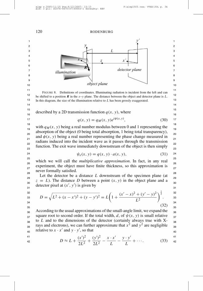
120 RODENBURG
1 1
2 2
3 3
4 4
5 5
6 6
7 7
8 8
9 9
10 10
11 11
12 12
13 13
14 14
15 15
16 16
17 17
18 18
19 19
20 20
21 21
22 22
23 23
24 24
25 25
26 26
27 27
28 28
29 29
30 30
31 31
32 32
33 33
34 34
35 35
36 36
37 37
38 38
39 39
40 40
41 41
42 42
FIGURE 8. Definitions of coordinates. Illuminating radiation is incident from the left and canbe shifted to a position R in the x–y plane. The distance between the object and detector plane is L.In this diagram, the size of the illumination relative to L has been grossly exaggerated.
described by a 2D transmission function q(x, y), where
q(x, y) = qM(x, y)ei!(x,y), (30)
with qM(x, y) being a real number modulus between 0 and 1 representing theabsorption of the object (0 being total absorption, 1 being total transparency),and !(x, y) being a real number representing the phase change measured inradians induced into the incident wave as it passes through the transmissionfunction. The exit wave immediately downstream of the object is then simply
$e(x, y) = q(x, y) · a(x, y), (31)
which we will call the multiplicative approximation. In fact, in any realexperiment, the object must have finite thickness, so this approximation isnever formally satisfied.
Let the detector be a distance L downstream of the specimen plane (atz = L). The distance D between a point (x, y) in the object plane and adetector pixel at (x$, y$) is given by
D =.
L2 + (x " x$)2 + (y " y$)2 = L
*1 + (x$ " x)2 + (y$ " y)2
L2
+ 12
.
(32)According to the usual approximations of the small-angle limit, we expand thesquare root to second order. If the total width, d , of $(x, y) is small relativeto L and to the dimensions of the detector (certainly always true with X-rays and electrons), we can further approximate that x2 and y2 are negligiblerelative to x · x$ and y · y$, so that
D ) L + (x$)2
2L2 + (y$)2
2L2 " x · x$
L" y · y$
L+ · · · . (33)
aiep v.2005/11/15 Prn:6/12/2007; 13:13 F:aiep1503.tex; VTEX/JOL p. 34aid: 3 pii: S1076-5670(07)00003-1 docsubty: REV
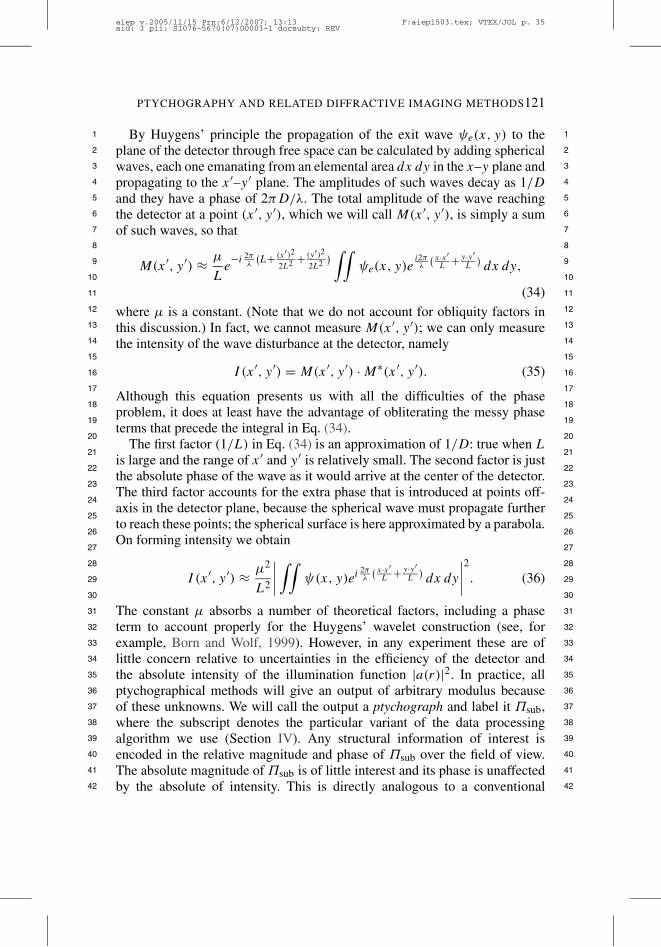
PTYCHOGRAPHY AND RELATED DIFFRACTIVE IMAGING METHODS121
1 1
2 2
3 3
4 4
5 5
6 6
7 7
8 8
9 9
10 10
11 11
12 12
13 13
14 14
15 15
16 16
17 17
18 18
19 19
20 20
21 21
22 22
23 23
24 24
25 25
26 26
27 27
28 28
29 29
30 30
31 31
32 32
33 33
34 34
35 35
36 36
37 37
38 38
39 39
40 40
41 41
42 42
By Huygens’ principle the propagation of the exit wave $e(x, y) to theplane of the detector through free space can be calculated by adding sphericalwaves, each one emanating from an elemental area dx dy in the x–y plane andpropagating to the x$–y$ plane. The amplitudes of such waves decay as 1/Dand they have a phase of 2"D/*. The total amplitude of the wave reachingthe detector at a point (x$, y$), which we will call M(x$, y$), is simply a sumof such waves, so that
M(x$, y$) ) µ
Le"i 2"
*
,L+ (x$)2
2L2 + (y$)22L2
- !!$e(x, y)e
i2"*
, x·x$L + y·y$
L
-dx dy,
(34)where µ is a constant. (Note that we do not account for obliquity factors inthis discussion.) In fact, we cannot measure M(x$, y$); we can only measurethe intensity of the wave disturbance at the detector, namely
I (x$, y$) = M(x$, y$) · M#(x$, y$). (35)
Although this equation presents us with all the difficulties of the phaseproblem, it does at least have the advantage of obliterating the messy phaseterms that precede the integral in Eq. (34).
The first factor (1/L) in Eq. (34) is an approximation of 1/D: true when Lis large and the range of x$ and y$ is relatively small. The second factor is justthe absolute phase of the wave as it would arrive at the center of the detector.The third factor accounts for the extra phase that is introduced at points off-axis in the detector plane, because the spherical wave must propagate furtherto reach these points; the spherical surface is here approximated by a parabola.On forming intensity we obtain
I (x$, y$) ) µ2
L2
''''
!!$(x, y)ei 2"
*
, x·x$L + y·y$
L
-dx dy
''''2
. (36)
The constant µ absorbs a number of theoretical factors, including a phaseterm to account properly for the Huygens’ wavelet construction (see, forexample, Born and Wolf, 1999). However, in any experiment these are oflittle concern relative to uncertainties in the efficiency of the detector andthe absolute intensity of the illumination function |a(r)|2. In practice, allptychographical methods will give an output of arbitrary modulus becauseof these unknowns. We will call the output a ptychograph and label it +sub,where the subscript denotes the particular variant of the data processingalgorithm we use (Section IV). Any structural information of interest isencoded in the relative magnitude and phase of +sub over the field of view.The absolute magnitude of +sub is of little interest and its phase is unaffectedby the absolute of intensity. This is directly analogous to a conventional
aiep v.2005/11/15 Prn:6/12/2007; 13:13 F:aiep1503.tex; VTEX/JOL p. 35aid: 3 pii: S1076-5670(07)00003-1 docsubty: REV

122 RODENBURG
1 1
2 2
3 3
4 4
5 5
6 6
7 7
8 8
9 9
10 10
11 11
12 12
13 13
14 14
15 15
16 16
17 17
18 18
19 19
20 20
21 21
22 22
23 23
24 24
25 25
26 26
27 27
28 28
29 29
30 30
31 31
32 32
33 33
34 34
35 35
36 36
37 37
38 38
39 39
40 40
41 41
42 42
microscope where the user has very little interest in the precise calibration ofthe brightness of the illumination, as long as it is sufficient to see the structuresof interest. Henceforth we will therefore ignore the constant terms µ/L.
For the purposes of our theory, we can further remove the physical effectsof the scaling of the diffraction pattern by the camera length L and thewavelength by changing the coordinates of the measurement plane to u )x$/*L and v ) y$/*L, and thus write
M(u, v) =!!
$(x, y)ei2"(x·u+y·v) dx dy (37)
or, more compactly,
M(u) =!
$(r)ei2"u·r dr = %$(r), (38)
where u is a 2D detector coordinate vector u = uu + vv, with u and v as unitvectors in reciprocal space; and r is a 2D vector in real space, r = xx + yy.
We can move our illumination function to a position defined by a 2Dvector R, so that
$(r) = a(r " R) · q(r). (39)
The complete ptychographical data set for 2D functions a and q is thendefined as the 4D intensity distribution
I (u,R) =''M(u,R)
''2 =''%
,a(r " R) · q(r)
-''2, (40)
which can be written as the ptychographical convolution
I (u,R) ='',A(u)ei2"R·u- & Q(u)
''2, (41)
where A(u) = %a(r) and Q(u) = %a(r). We will call this the fundamentalptychographic equation.
These equations are the basis of all the theory of both the “direct” de-convolution methods developed by the Cambridge group in the 1990s (seeSections IV.A, IV.B, and IV.D) and the iterative solutions to the ptychograph-ical data set (see Section IV.C). The nomenclature of the Cambridge workwas borrowed from the image processing literature: R was named !,u wasnamed r $, and the reciprocal of ! was named !$, which we will call r . Thebiggest potential source of confusion is that what we will call U (the backFourier transform coordinate of u) was formerly named r . The rationale ofthis altered nomenclature is to unify it with the reciprocal u–v coordinateswidely used by Cowley and others (e.g., Cowley, 1995). Furthermore, theuse of the dashed nomenclature for reciprocal coordinates becomes clumsyin thinking of 3D scattering in terms of the existing TEM nomenclature
aiep v.2005/11/15 Prn:6/12/2007; 13:13 F:aiep1503.tex; VTEX/JOL p. 36aid: 3 pii: S1076-5670(07)00003-1 docsubty: REV

PTYCHOGRAPHY AND RELATED DIFFRACTIVE IMAGING METHODS123
1 1
2 2
3 3
4 4
5 5
6 6
7 7
8 8
9 9
10 10
11 11
12 12
13 13
14 14
15 15
16 16
17 17
18 18
19 19
20 20
21 21
22 22
23 23
24 24
25 25
26 26
27 27
28 28
29 29
30 30
31 31
32 32
33 33
34 34
35 35
36 36
37 37
38 38
39 39
40 40
41 41
42 42
(Section III.B). Note that the function a(r) was in some earlier articles (e.g.,Rodenburg and Bates, 1992) called P(r) – equivalent to the “probe” functionin STEM.
Perhaps a rather misleading nomenclature in this former schema was tocall the object function $(r) (which we have called here the transmissionfunction q(r)). The author’s intention was to suggest that the function we wereaiming to solve for was the exit wave as it would appear under plane waveillumination perpendicular to the (infinitesimally thin) object. However, thisled to some misunderstanding because many colleagues in the field of electronscattering supposed that this was also meant to represent the exit wave asit would appear (under plane wave illumination) from a thick object. Sincethe exit wave in electron microscopy arising from thick, strongly scatteringobjects bears no obvious relationship to the form of the scattering potentialin the object (especially given a range of incident vectors necessary to form alocalized probe), much of this work was dismissed as being based on a simplywrong assumption, or that the method could only possibly work for thin,weak, kinematically scattering objects. In fact, ptychography is remarkablyrobust to dynamical scattering and thickness effects even in the case ofcrystalline objects of small unit cell (Plamann and Rodenburg, 1998), forreasons discussed briefly in Section IV.A.
B. Three-Dimensional Geometry
Another way of thinking of the integral in Eq. (36) is via Fig. 9(a). TheFraunhofer approximation is equivalent to saying that only parallel beamsscattered from the object interfere with one another. It is easy to show thatthis condition is met if
L * d2
*. (42)
If we say that in the absence of the transmission function the phase of theHuygens’ wavelet emanating from x = y = z = 0 is zero, then the extraphase introduced to a beam (or ray) emanating from a point (x, y) at z = 0(that is, from within the 2D) is determined only by the two orthogonal angles,x and ,y . ,x is the angle between the plane x = 0 and the plane containingboth the y axis and the line of the ray in question (as shown in Fig. 9(b)); ,y isdefined similarly with respect to the plane y = 0. If we redefine
u = sin ,x
*(43a)
and
v = sin ,y
*, (43b)
aiep v.2005/11/15 Prn:6/12/2007; 13:13 F:aiep1503.tex; VTEX/JOL p. 37aid: 3 pii: S1076-5670(07)00003-1 docsubty: REV

124 RODENBURG
1 1
2 2
3 3
4 4
5 5
6 6
7 7
8 8
9 9
10 10
11 11
12 12
13 13
14 14
15 15
16 16
17 17
18 18
19 19
20 20
21 21
22 22
23 23
24 24
25 25
26 26
27 27
28 28
29 29
30 30
31 31
32 32
33 33
34 34
35 35
36 36
37 37
38 38
39 39
40 40
41 41
42 42
(a)
(b)
FIGURE 9. (a) Parallel beams scattered by the object will meet up and interfere in theFraunhofer diffraction plane. For this 1D object, the path length of the beam emanating from theelemental length dx positioned at x is shorter than the beam scattered at the origin by an amountx · sin ,x , and consequently has an extra phase change 2"x · sin ,x/*, relative to the waves scatteredfrom x = 0. By substitution from Eq. (43a), the total resultant amplitude is hence the Fourier transformF(u) =
"f (x)ei2"ux dx, where f (x) is the exit wave immediately downstream of the object. For a
3D object, similar arguments lead to Eq. (45). (b) Definition of ,x . The heavy arrow subtends fromthe specimen to a detector pixel. ,x is the angle between the plane x = 0 and the plane containing theheavy arrow and the y-axis.
then, with reference to Fig. 9(a), the resulting integral of all such beams overthe exit wave is identical to Eq. (37). These rectilinear angular coordinateshave the advantage of being correct at all (large) angles where 3D scatteringeffects dominate. We can think of the far-field scattered wave function asexisting over a spherical hemisphere (Fig. 10(a)), of diameter L (satisfyingEq. (42)). We index the coordinates on this surface by the coordinates u and v.In Fig. 10(b) we draw the view of this hemisphere looking back at it from a
aiep v.2005/11/15 Prn:6/12/2007; 13:13 F:aiep1503.tex; VTEX/JOL p. 38aid: 3 pii: S1076-5670(07)00003-1 docsubty: REV
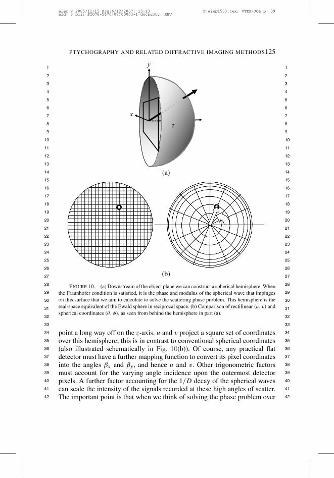
PTYCHOGRAPHY AND RELATED DIFFRACTIVE IMAGING METHODS125
1 1
2 2
3 3
4 4
5 5
6 6
7 7
8 8
9 9
10 10
11 11
12 12
13 13
14 14
15 15
16 16
17 17
18 18
19 19
20 20
21 21
22 22
23 23
24 24
25 25
26 26
27 27
28 28
29 29
30 30
31 31
32 32
33 33
34 34
35 35
36 36
37 37
38 38
39 39
40 40
41 41
42 42
(a)
(b)
FIGURE 10. (a) Downstream of the object plane we can construct a spherical hemisphere. Whenthe Fraunhofer condition is satisfied, it is the phase and modulus of the spherical wave that impingeson this surface that we aim to calculate to solve the scattering phase problem. This hemisphere is thereal-space equivalent of the Ewald sphere in reciprocal space. (b) Comparison of rectilinear (u, v) andspherical coordinates (-,!), as seen from behind the hemisphere in part (a).
point a long way off on the z-axis. u and v project a square set of coordinatesover this hemisphere; this is in contrast to conventional spherical coordinates(also illustrated schematically in Fig. 10(b)). Of course, any practical flatdetector must have a further mapping function to convert its pixel coordinatesinto the angles ,x and ,y , and hence u and v. Other trigonometric factorsmust account for the varying angle incidence upon the outermost detectorpixels. A further factor accounting for the 1/D decay of the spherical wavescan scale the intensity of the signals recorded at these high angles of scatter.The important point is that when we think of solving the phase problem over
aiep v.2005/11/15 Prn:6/12/2007; 13:13 F:aiep1503.tex; VTEX/JOL p. 39aid: 3 pii: S1076-5670(07)00003-1 docsubty: REV

126 RODENBURG
1 1
2 2
3 3
4 4
5 5
6 6
7 7
8 8
9 9
10 10
11 11
12 12
13 13
14 14
15 15
16 16
17 17
18 18
19 19
20 20
21 21
22 22
23 23
24 24
25 25
26 26
27 27
28 28
29 29
30 30
31 31
32 32
33 33
34 34
35 35
36 36
37 37
38 38
39 39
40 40
41 41
42 42
the entire range of scattering angles available, then the phase we are trying tosolve manifests itself in the absolute phase of the spherical wave that impingesupon this hemispherical surface, and that when our processing involves arectilinear detector and data manipulations involving fast Fourier transformsof functions sampled on equally spaced arrays, then it is very convenient tofirst map the detected intensities onto the coordinates u and v. We assume thismapping in all that follows.
Once we begin to deal with high scattering angles, then implicitly the 2Dtransmission object function also breaks down. Quite simply, if we look ata 3D object from a number of different angles, then the features on the topand bottom surfaces of the object appear to move with respect to one another.In this section, vector quantities r and k will always be 3D (in contrast tothe previous section) and will sometimes be written in terms of coordinates(x, y, z) and (u, v,w, ) respectively.
Let the object in three dimensions be a function V (r); its 3D Fouriertransform is
F(k) = c
!V (r)e2"k·r dr, (44)
where c is a constant. k is a 3D vector in reciprocal space that can bedecomposed into unit vectors k = uu + vv + ww. (Note that the vector uwill be reserved for the 2D detector vector coordinate u = uu + vv.) In thescalar theory of light optics, V (r) is called the optical potential. In electronscattering theory, V (r) is the spatial distribution of the atomic potential in theobject, measured in volts. V (r) can be complex, the imaginary componentsrepresenting absorption of the radiation. The perfect imaging machine wouldaim to estimate accurately, and at very high resolution, V (r).
V (r) must be estimated from knowledge of the distribution of the incidentradiation, which has k-vectors that will call ki , and the scattered radiation,which has k-vectors we will call ks . If the object is strongly scattering orthick, then the incident waves striking parts of it some distance from theentrance surface will be substantially different from what would have arrivedat that region had the illumination function been allowed to propagate throughfree space. Under these circumstances the inference of V (r) is in generalnontrivial, even if the modulus and phase of the scattered radiation can bemeasured or calculated perfectly.
If the object scatters weakly (whether or not it is thick), then we can usethe first Born approximation (Mott and Massey, 1965). That is to say, theintensity of the incident beam is not substantially attenuated as a result ofpassing through the object and the total intensity scattered away from thedirection of the incident beam is relatively low. We will discuss this (so-calledkinematical) approximation in the next section, as well as its relationship to
aiep v.2005/11/15 Prn:6/12/2007; 13:13 F:aiep1503.tex; VTEX/JOL p. 40aid: 3 pii: S1076-5670(07)00003-1 docsubty: REV
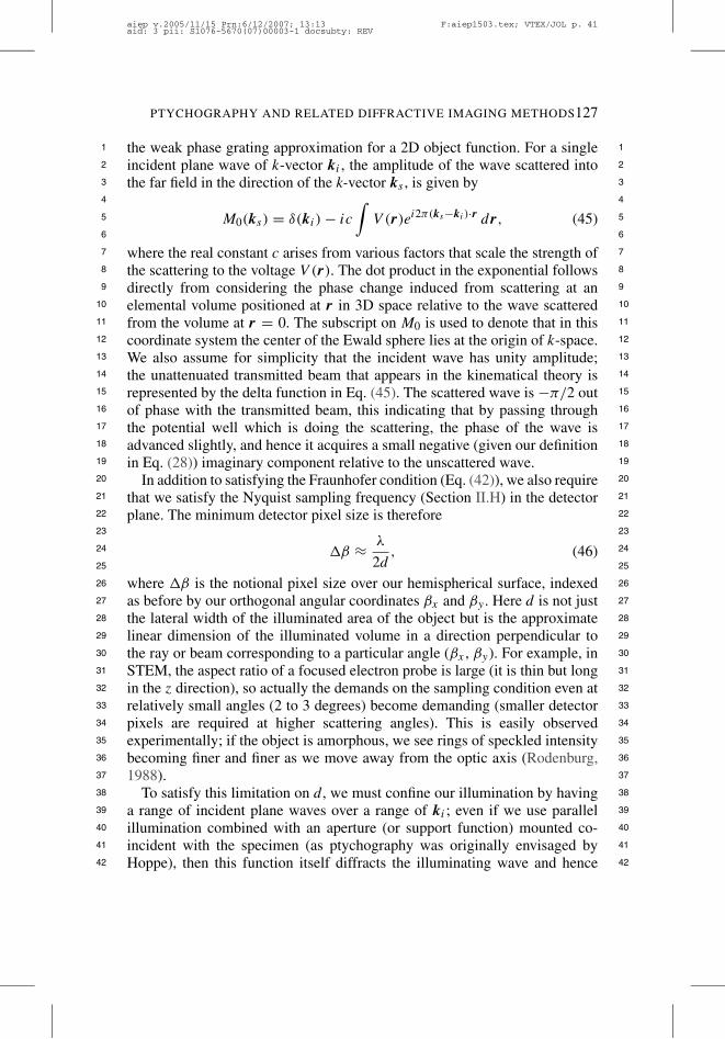
PTYCHOGRAPHY AND RELATED DIFFRACTIVE IMAGING METHODS127
1 1
2 2
3 3
4 4
5 5
6 6
7 7
8 8
9 9
10 10
11 11
12 12
13 13
14 14
15 15
16 16
17 17
18 18
19 19
20 20
21 21
22 22
23 23
24 24
25 25
26 26
27 27
28 28
29 29
30 30
31 31
32 32
33 33
34 34
35 35
36 36
37 37
38 38
39 39
40 40
41 41
42 42
the weak phase grating approximation for a 2D object function. For a singleincident plane wave of k-vector ki , the amplitude of the wave scattered intothe far field in the direction of the k-vector ks , is given by
M0(ks) = '(ki ) " ic
!V (r)ei2"(ks"ki )·r dr, (45)
where the real constant c arises from various factors that scale the strength ofthe scattering to the voltage V (r). The dot product in the exponential followsdirectly from considering the phase change induced from scattering at anelemental volume positioned at r in 3D space relative to the wave scatteredfrom the volume at r = 0. The subscript on M0 is used to denote that in thiscoordinate system the center of the Ewald sphere lies at the origin of k-space.We also assume for simplicity that the incident wave has unity amplitude;the unattenuated transmitted beam that appears in the kinematical theory isrepresented by the delta function in Eq. (45). The scattered wave is ""/2 outof phase with the transmitted beam, this indicating that by passing throughthe potential well which is doing the scattering, the phase of the wave isadvanced slightly, and hence it acquires a small negative (given our definitionin Eq. (28)) imaginary component relative to the unscattered wave.
In addition to satisfying the Fraunhofer condition (Eq. (42)), we also requirethat we satisfy the Nyquist sampling frequency (Section II.H) in the detectorplane. The minimum detector pixel size is therefore
&, ) *
2d, (46)
where &, is the notional pixel size over our hemispherical surface, indexedas before by our orthogonal angular coordinates ,x and ,y . Here d is not justthe lateral width of the illuminated area of the object but is the approximatelinear dimension of the illuminated volume in a direction perpendicular tothe ray or beam corresponding to a particular angle (,x , ,y). For example, inSTEM, the aspect ratio of a focused electron probe is large (it is thin but longin the z direction), so actually the demands on the sampling condition even atrelatively small angles (2 to 3 degrees) become demanding (smaller detectorpixels are required at higher scattering angles). This is easily observedexperimentally; if the object is amorphous, we see rings of speckled intensitybecoming finer and finer as we move away from the optic axis (Rodenburg,1988).
To satisfy this limitation on d , we must confine our illumination by havinga range of incident plane waves over a range of ki ; even if we use parallelillumination combined with an aperture (or support function) mounted co-incident with the specimen (as ptychography was originally envisaged byHoppe), then this function itself diffracts the illuminating wave and hence
aiep v.2005/11/15 Prn:6/12/2007; 13:13 F:aiep1503.tex; VTEX/JOL p. 41aid: 3 pii: S1076-5670(07)00003-1 docsubty: REV
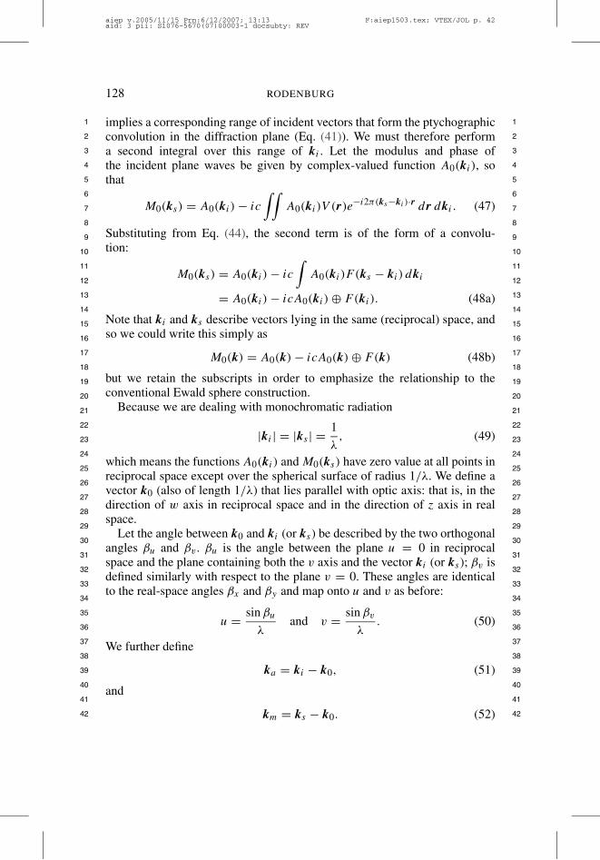
128 RODENBURG
1 1
2 2
3 3
4 4
5 5
6 6
7 7
8 8
9 9
10 10
11 11
12 12
13 13
14 14
15 15
16 16
17 17
18 18
19 19
20 20
21 21
22 22
23 23
24 24
25 25
26 26
27 27
28 28
29 29
30 30
31 31
32 32
33 33
34 34
35 35
36 36
37 37
38 38
39 39
40 40
41 41
42 42
implies a corresponding range of incident vectors that form the ptychographicconvolution in the diffraction plane (Eq. (41)). We must therefore performa second integral over this range of ki . Let the modulus and phase ofthe incident plane waves be given by complex-valued function A0(ki ), sothat
M0(ks) = A0(ki ) " ic
!!A0(ki )V (r)e"i2"(ks"ki )·r dr dki . (47)
Substituting from Eq. (44), the second term is of the form of a convolu-tion:
M0(ks) = A0(ki ) " ic
!A0(ki )F (ks " ki ) dki
= A0(ki ) " icA0(ki ) & F(ki ). (48a)
Note that ki and ks describe vectors lying in the same (reciprocal) space, andso we could write this simply as
M0(k) = A0(k) " icA0(k) & F(k) (48b)
but we retain the subscripts in order to emphasize the relationship to theconventional Ewald sphere construction.
Because we are dealing with monochromatic radiation
|ki | = |ks | = 1*, (49)
which means the functions A0(ki ) and M0(ks) have zero value at all points inreciprocal space except over the spherical surface of radius 1/*. We define avector k0 (also of length 1/*) that lies parallel with optic axis: that is, in thedirection of w axis in reciprocal space and in the direction of z axis in realspace.
Let the angle between k0 and ki (or ks) be described by the two orthogonalangles ,u and ,v . ,u is the angle between the plane u = 0 in reciprocalspace and the plane containing both the v axis and the vector ki (or ks); ,v isdefined similarly with respect to the plane v = 0. These angles are identicalto the real-space angles ,x and ,y and map onto u and v as before:
u = sin ,u
*and v = sin ,v
*. (50)
We further define
ka = ki " k0, (51)
and
km = ks " k0. (52)
aiep v.2005/11/15 Prn:6/12/2007; 13:13 F:aiep1503.tex; VTEX/JOL p. 42aid: 3 pii: S1076-5670(07)00003-1 docsubty: REV
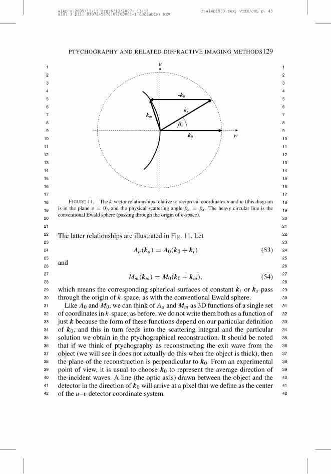
PTYCHOGRAPHY AND RELATED DIFFRACTIVE IMAGING METHODS129
1 1
2 2
3 3
4 4
5 5
6 6
7 7
8 8
9 9
10 10
11 11
12 12
13 13
14 14
15 15
16 16
17 17
18 18
19 19
20 20
21 21
22 22
23 23
24 24
25 25
26 26
27 27
28 28
29 29
30 30
31 31
32 32
33 33
34 34
35 35
36 36
37 37
38 38
39 39
40 40
41 41
42 42
FIGURE 11. The k-vector relationships relative to reciprocal coordinates u and w (this diagramis in the plane v = 0), and the physical scattering angle ,u = ,x . The heavy circular line is theconventional Ewald sphere (passing through the origin of k-space).
The latter relationships are illustrated in Fig. 11. Let
Aa(ka) = A0(k0 + ki ) (53)
and
Mm(km) = M0(k0 + km), (54)
which means the corresponding spherical surfaces of constant ki or ks passthrough the origin of k-space, as with the conventional Ewald sphere.
Like A0 and M0, we can think of Aa and Mm as 3D functions of a single setof coordinates in k-space; as before, we do not write them both as a function ofjust k because the form of these functions depend on our particular definitionof k0, and this in turn feeds into the scattering integral and the particularsolution we obtain in the ptychographical reconstruction. It should be notedthat if we think of ptychography as reconstructing the exit wave from theobject (we will see it does not actually do this when the object is thick), thenthe plane of the reconstruction is perpendicular to k0. From an experimentalpoint of view, it is usual to choose k0 to represent the average direction ofthe incident waves. A line (the optic axis) drawn between the object and thedetector in the direction of k0 will arrive at a pixel that we define as the centerof the u–v detector coordinate system.
aiep v.2005/11/15 Prn:6/12/2007; 13:13 F:aiep1503.tex; VTEX/JOL p. 43aid: 3 pii: S1076-5670(07)00003-1 docsubty: REV
130 RODENBURG
1 1
2 2
3 3
4 4
5 5
6 6
7 7
8 8
9 9
10 10
11 11
12 12
13 13
14 14
15 15
16 16
17 17
18 18
19 19
20 20
21 21
22 22
23 23
24 24
25 25
26 26
27 27
28 28
29 29
30 30
31 31
32 32
33 33
34 34
35 35
36 36
37 37
38 38
39 39
40 40
41 41
42 42
Now both Aa(ka) and Mm(km) only have a value over the Ewald sphere.We define a function .(u, v,w) which of the form of a “spherical deltafunction” in reciprocal space so that it satisfies (for any function G(k)),
!G(k).(kw " k) dk =
)G(k) for k = kw,
0 for k '= kw,(55)
where, for given values of u and v, kw is constrained to the locus of points
kw = uu + vv + 1*
,,1 " *2,u2 + v2-- 1
2 " 1-w. (56)
(The unit vector u should not be confused with the 2D detector vector u.)We can describe fully the 3D functions Aa(ka) and Mm(km) by the 2D
complex functions A(u) and M(u), where
A(u) = A(u, v) = .(u, v,w) · Aa(ka) (57)
and
M(u) = M(u, v) = .(u, v,w) · Mm(km), (58)
where it must be remembered that u, v uniquely define w via Eq. (56). Thescattering Eqs. (48a) and (48b) now become
Mm(km) = Aa(ka) " ic
!Aa(ka)F (km " ka) dka (59)
or
M(u) = .(k) ·%Aa(k) " icAa(k) & F(k)
&. (60)
In the object space we have a 3D illumination function a(r), which at z = 0is simply the addition of the incident plane waves defined by the amplitudesA(u), that is,
P(x, y, 0) =!!
A(u, v)e"i2"(u·x+v·y) du dv = %"1A(u). (61)
If the illumination is physically created by a lens (as in the STEM geometry),then the phase of A(u) will depend on its aberrations.
Let us suppose that the lens is perfect. In the absence of a specimen, wesimply have the transmitted beam in the detector plane, so that I (u) = M(u) ·M#(u) = A(u)A#(u) and so it is somewhat meaningless to worry about theexact z (or x, y) displacement of a(r). However, as soon as we introduce aspecimen, its position in the z-direction will strongly affect M(u). How is thisreflected in Eq. (60)? For kinematical scattering, in real space have a(r) plusa term "ic · a(r) · V (r), the latter being a source of waves scattered by thepotential, "/2 out of phase with the illuminating function.
aiep v.2005/11/15 Prn:6/12/2007; 13:13 F:aiep1503.tex; VTEX/JOL p. 44aid: 3 pii: S1076-5670(07)00003-1 docsubty: REV

PTYCHOGRAPHY AND RELATED DIFFRACTIVE IMAGING METHODS131
1 1
2 2
3 3
4 4
5 5
6 6
7 7
8 8
9 9
10 10
11 11
12 12
13 13
14 14
15 15
16 16
17 17
18 18
19 19
20 20
21 21
22 22
23 23
24 24
25 25
26 26
27 27
28 28
29 29
30 30
31 31
32 32
33 33
34 34
35 35
36 36
37 37
38 38
39 39
40 40
41 41
42 42
Let us consider a single scattering center positioned at x = y = z = 0. Ifwe shift the illuminating beam by a distance of z0 along the optic axis, thenwe would expect to see a propagated illumination function P(x, y, y " z0)incident upon this scattering center. By the Fourier shift theorem, our 3Dfunction representing the probe in reciprocal space now has a phase changeintroduced into it of ei! , where ! = 2"z0w. This means that when we formA(u) via Eq. (60), the dependence of w on u and v will introduce a phasechange in A(u) equal to
! = z02"
*
,,1 " *2,u2 + v2-- 1
2 " 1-, (62)
which, for small values of u and v, approximates to the familiar defocus term
! ) z0*",u2 + v2-. (63)
In other words, the phase change induced in reciprocal space as a result ofa z-direction displacement of the specimen or probe function is equivalentto a defocus term when this shift is expressed in reciprocal space over thecurvature of the Ewald sphere.
To clarify this scattering geometry in terms of the conventional Ewaldsphere construction, we refer to Fig. 12. Once we have defined k0, then the
FIGURE 12. For a particular incident plane wave (e.g., ki as shown) and scattering vector, ks ,the amplitude of scattered wave is given by the value of F(k) at the center of the small, gray circle. Infact, there is a range of incident vectors; hence the amplitude at any one scattering direction ks is theintegral over the surface S in F(k).
aiep v.2005/11/15 Prn:6/12/2007; 13:13 F:aiep1503.tex; VTEX/JOL p. 45aid: 3 pii: S1076-5670(07)00003-1 docsubty: REV
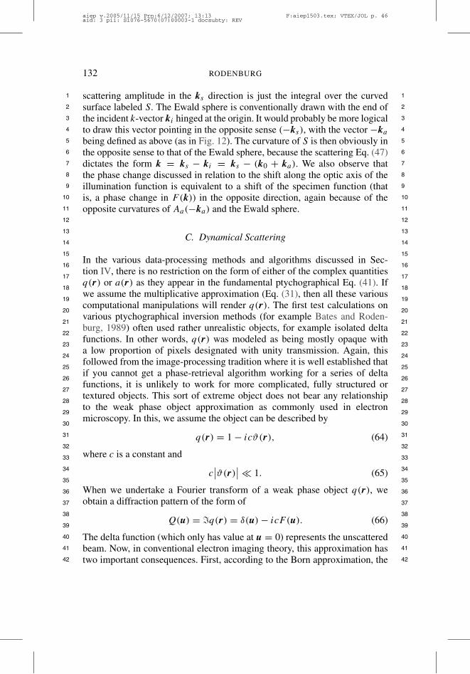
132 RODENBURG
1 1
2 2
3 3
4 4
5 5
6 6
7 7
8 8
9 9
10 10
11 11
12 12
13 13
14 14
15 15
16 16
17 17
18 18
19 19
20 20
21 21
22 22
23 23
24 24
25 25
26 26
27 27
28 28
29 29
30 30
31 31
32 32
33 33
34 34
35 35
36 36
37 37
38 38
39 39
40 40
41 41
42 42
scattering amplitude in the ks direction is just the integral over the curvedsurface labeled S. The Ewald sphere is conventionally drawn with the end ofthe incident k-vector ki hinged at the origin. It would probably be more logicalto draw this vector pointing in the opposite sense ("ks), with the vector "ka
being defined as above (as in Fig. 12). The curvature of S is then obviously inthe opposite sense to that of the Ewald sphere, because the scattering Eq. (47)dictates the form k = ks " ki = ks " (k0 + ka). We also observe thatthe phase change discussed in relation to the shift along the optic axis of theillumination function is equivalent to a shift of the specimen function (thatis, a phase change in F(k)) in the opposite direction, again because of theopposite curvatures of Aa("ka) and the Ewald sphere.
C. Dynamical Scattering
In the various data-processing methods and algorithms discussed in Sec-tion IV, there is no restriction on the form of either of the complex quantitiesq(r) or a(r) as they appear in the fundamental ptychographical Eq. (41). Ifwe assume the multiplicative approximation (Eq. (31), then all these variouscomputational manipulations will render q(r). The first test calculations onvarious ptychographical inversion methods (for example Bates and Roden-burg, 1989) often used rather unrealistic objects, for example isolated deltafunctions. In other words, q(r) was modeled as being mostly opaque witha low proportion of pixels designated with unity transmission. Again, thisfollowed from the image-processing tradition where it is well established thatif you cannot get a phase-retrieval algorithm working for a series of deltafunctions, it is unlikely to work for more complicated, fully structured ortextured objects. This sort of extreme object does not bear any relationshipto the weak phase object approximation as commonly used in electronmicroscopy. In this, we assume the object can be described by
q(r) = 1 " ic/(r), (64)
where c is a constant and
c''/(r)
'' + 1. (65)
When we undertake a Fourier transform of a weak phase object q(r), weobtain a diffraction pattern of the form of
Q(u) = %q(r) = '(u) " icF (u). (66)
The delta function (which only has value at u = 0) represents the unscatteredbeam. Now, in conventional electron imaging theory, this approximation hastwo important consequences. First, according to the Born approximation, the
aiep v.2005/11/15 Prn:6/12/2007; 13:13 F:aiep1503.tex; VTEX/JOL p. 46aid: 3 pii: S1076-5670(07)00003-1 docsubty: REV
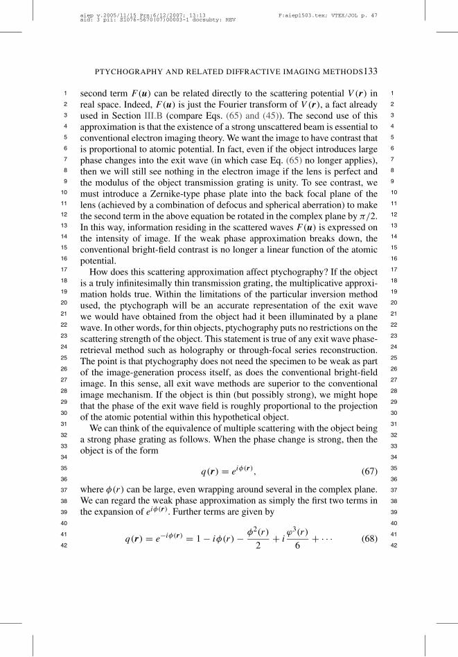
PTYCHOGRAPHY AND RELATED DIFFRACTIVE IMAGING METHODS133
1 1
2 2
3 3
4 4
5 5
6 6
7 7
8 8
9 9
10 10
11 11
12 12
13 13
14 14
15 15
16 16
17 17
18 18
19 19
20 20
21 21
22 22
23 23
24 24
25 25
26 26
27 27
28 28
29 29
30 30
31 31
32 32
33 33
34 34
35 35
36 36
37 37
38 38
39 39
40 40
41 41
42 42
second term F(u) can be related directly to the scattering potential V (r) inreal space. Indeed, F(u) is just the Fourier transform of V (r), a fact alreadyused in Section III.B (compare Eqs. (65) and (45)). The second use of thisapproximation is that the existence of a strong unscattered beam is essential toconventional electron imaging theory. We want the image to have contrast thatis proportional to atomic potential. In fact, even if the object introduces largephase changes into the exit wave (in which case Eq. (65) no longer applies),then we will still see nothing in the electron image if the lens is perfect andthe modulus of the object transmission grating is unity. To see contrast, wemust introduce a Zernike-type phase plate into the back focal plane of thelens (achieved by a combination of defocus and spherical aberration) to makethe second term in the above equation be rotated in the complex plane by "/2.In this way, information residing in the scattered waves F(u) is expressed onthe intensity of image. If the weak phase approximation breaks down, theconventional bright-field contrast is no longer a linear function of the atomicpotential.
How does this scattering approximation affect ptychography? If the objectis a truly infinitesimally thin transmission grating, the multiplicative approxi-mation holds true. Within the limitations of the particular inversion methodused, the ptychograph will be an accurate representation of the exit wavewe would have obtained from the object had it been illuminated by a planewave. In other words, for thin objects, ptychography puts no restrictions on thescattering strength of the object. This statement is true of any exit wave phase-retrieval method such as holography or through-focal series reconstruction.The point is that ptychography does not need the specimen to be weak as partof the image-generation process itself, as does the conventional bright-fieldimage. In this sense, all exit wave methods are superior to the conventionalimage mechanism. If the object is thin (but possibly strong), we might hopethat the phase of the exit wave field is roughly proportional to the projectionof the atomic potential within this hypothetical object.
We can think of the equivalence of multiple scattering with the object beinga strong phase grating as follows. When the phase change is strong, then theobject is of the form
q(r) = ei!(r), (67)
where !(r) can be large, even wrapping around several in the complex plane.We can regard the weak phase approximation as simply the first two terms inthe expansion of ei!(r). Further terms are given by
q(r) = e"i!(r) = 1 " i!(r) " !2(r)
2+ i
03(r)
6+ · · · (68)
aiep v.2005/11/15 Prn:6/12/2007; 13:13 F:aiep1503.tex; VTEX/JOL p. 47aid: 3 pii: S1076-5670(07)00003-1 docsubty: REV

134 RODENBURG
1 1
2 2
3 3
4 4
5 5
6 6
7 7
8 8
9 9
10 10
11 11
12 12
13 13
14 14
15 15
16 16
17 17
18 18
19 19
20 20
21 21
22 22
23 23
24 24
25 25
26 26
27 27
28 28
29 29
30 30
31 31
32 32
33 33
34 34
35 35
36 36
37 37
38 38
39 39
40 40
41 41
42 42
so that means that the Fourier transform is (using the convolution theorem)
Q(u) = '(u) " i1(r) " 121(r) & 1(r)
+ i
61(r) & 1(r) & 1(r) + · · · . (69)
The higher-order terms are the diffraction pattern convolved with itself; theseterms represent the multiple scattering. All the beams in the diffraction patterncan act as a source of a new diffraction pattern centered on that beam.
Our problems therefore do not arise from dynamical scattering per se,but from the 3D scattering (as in Section III.B) combined with dynamicalscattering. Think of this in terms of a multislice calculation. Suppose wesimply switch off the propagation term introduced between each elementalweak phase grating. The result is just a product of all the weak phase changesintroduced by each layer of the object (Fig. 13). This is simply
$e(r) = ei01(r)ei02(r)ei03(r)ei04(r)ei05(r)ei06(r) · · · , (70)
where the 0j (r) is the weak phase change induced by j th slice. A wavecomponent of a high-energy electron traveling in one dimension in the z-direction over a potential well will accumulate phase relative to a wavecomponent that does not pass over the same well. This is really the Wentzel–Kramers–Brillouin (WKB) approximation in quantum mechanics, whichbreaks down when there are sharp discontinuities in the potential or when thewell is deep. If our infinitesimally thin, strong object physically existed, thisapproximation would indeed break down. The exact solution would requirematching the amplitude and the gradient of the amplitude of the wave functionat the entrance and exit surfaces, leading to backscattered waves, and we canno longer approximate that the k-vector of the high-energy electron linearlyincreases as function of the potential well depth.
It is important to emphasize that ptychography does not solve for theexit wave when the object is thick; in other words, a ptychograph willnever provide the same modulus and phase as holography or through-focalseries reconstruction, because it explores a different (indeed, more extensive)volume of reciprocal space. With reference to Fig. 14, a conventional imageintegrates the complex function lying over a circular region of the Ewaldsphere, which is accommodated by the diaphragm of the imaging-forminglens. This integral is only identical to the ptychographic reconstruction whenthe object is so thin that all reciprocal features lying in the u–v plane arestretched out in the w-direction so much so that the integral over S is identicalto the integral C over the Ewald sphere.
Once we allow propagation effects, understanding what is going to happento the ptychograph is difficult. The theory of this has not been fully developed,
aiep v.2005/11/15 Prn:6/12/2007; 13:13 F:aiep1503.tex; VTEX/JOL p. 48aid: 3 pii: S1076-5670(07)00003-1 docsubty: REV
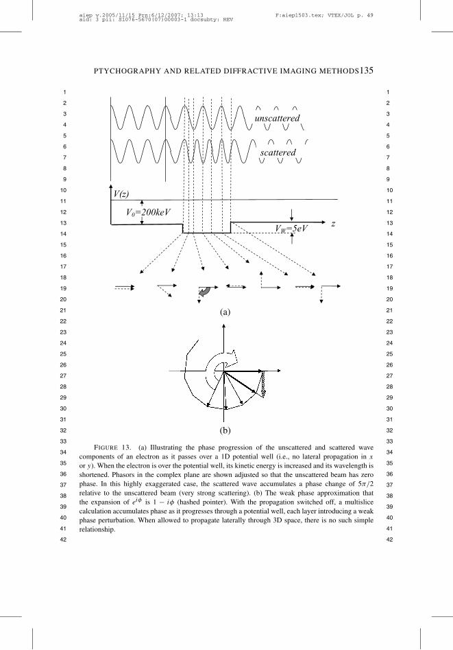
PTYCHOGRAPHY AND RELATED DIFFRACTIVE IMAGING METHODS135
1 1
2 2
3 3
4 4
5 5
6 6
7 7
8 8
9 9
10 10
11 11
12 12
13 13
14 14
15 15
16 16
17 17
18 18
19 19
20 20
21 21
22 22
23 23
24 24
25 25
26 26
27 27
28 28
29 29
30 30
31 31
32 32
33 33
34 34
35 35
36 36
37 37
38 38
39 39
40 40
41 41
42 42
(a)
(b)
FIGURE 13. (a) Illustrating the phase progression of the unscattered and scattered wavecomponents of an electron as it passes over a 1D potential well (i.e., no lateral propagation in x
or y). When the electron is over the potential well, its kinetic energy is increased and its wavelength isshortened. Phasors in the complex plane are shown adjusted so that the unscattered beam has zerophase. In this highly exaggerated case, the scattered wave accumulates a phase change of 5"/2relative to the unscattered beam (very strong scattering). (b) The weak phase approximation thatthe expansion of ei! is 1 " i! (hashed pointer). With the propagation switched off, a multislicecalculation accumulates phase as it progresses through a potential well, each layer introducing a weakphase perturbation. When allowed to propagate laterally through 3D space, there is no such simplerelationship.
aiep v.2005/11/15 Prn:6/12/2007; 13:13 F:aiep1503.tex; VTEX/JOL p. 49aid: 3 pii: S1076-5670(07)00003-1 docsubty: REV

136 RODENBURG
1 1
2 2
3 3
4 4
5 5
6 6
7 7
8 8
9 9
10 10
11 11
12 12
13 13
14 14
15 15
16 16
17 17
18 18
19 19
20 20
21 21
22 22
23 23
24 24
25 25
26 26
27 27
28 28
29 29
30 30
31 31
32 32
33 33
34 34
35 35
36 36
37 37
38 38
39 39
40 40
41 41
42 42
(a)
(b)
FIGURE 14. The integral over Ewald sphere, C, forms one image pixel in a conventionalmicroscope. The lens acts to integrate the scattered waves falling within the lens diaphragm(lower diagram). Ptychography integrates over surface S (see Fig. 12). The various ptychographicreconstructions effectively deconvolve the surface C to derive a single amplitude at point P , andhence an estimate of S. +lc (Section IV.A) relies on S embracing only one or two reflections at anyone position P . +p (Section IV.B) separates pairs of beams by Fourier transforming with respect to theprobe position. +" (Section IV.C) performs a division in real space. +W (Section IV.D) deconvolvesC via the Fourier transform of its intensity, H .
although Plamann and Rodenburg (1998) have compared model ptycho-graphical calculations with second-order dynamical scattering theory. Theseshow that even for strongly crystalline objects ptychography is in fact notas sensitive to thickness and dynamical effects as we might at first suppose.At 100 keV in silicon, the phase of the +lc ptychograph (see Section IV.A)
aiep v.2005/11/15 Prn:6/12/2007; 13:13 F:aiep1503.tex; VTEX/JOL p. 50aid: 3 pii: S1076-5670(07)00003-1 docsubty: REV
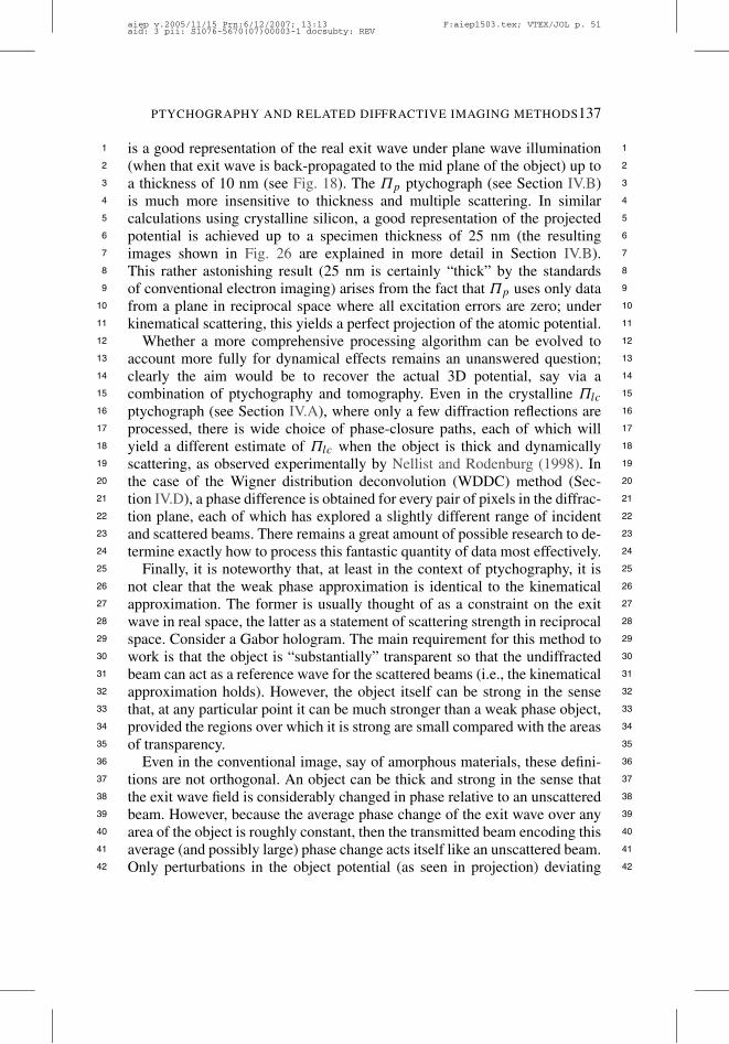
PTYCHOGRAPHY AND RELATED DIFFRACTIVE IMAGING METHODS137
1 1
2 2
3 3
4 4
5 5
6 6
7 7
8 8
9 9
10 10
11 11
12 12
13 13
14 14
15 15
16 16
17 17
18 18
19 19
20 20
21 21
22 22
23 23
24 24
25 25
26 26
27 27
28 28
29 29
30 30
31 31
32 32
33 33
34 34
35 35
36 36
37 37
38 38
39 39
40 40
41 41
42 42
is a good representation of the real exit wave under plane wave illumination(when that exit wave is back-propagated to the mid plane of the object) up toa thickness of 10 nm (see Fig. 18). The +p ptychograph (see Section IV.B)is much more insensitive to thickness and multiple scattering. In similarcalculations using crystalline silicon, a good representation of the projectedpotential is achieved up to a specimen thickness of 25 nm (the resultingimages shown in Fig. 26 are explained in more detail in Section IV.B).This rather astonishing result (25 nm is certainly “thick” by the standardsof conventional electron imaging) arises from the fact that +p uses only datafrom a plane in reciprocal space where all excitation errors are zero; underkinematical scattering, this yields a perfect projection of the atomic potential.
Whether a more comprehensive processing algorithm can be evolved toaccount more fully for dynamical effects remains an unanswered question;clearly the aim would be to recover the actual 3D potential, say via acombination of ptychography and tomography. Even in the crystalline +lc
ptychograph (see Section IV.A), where only a few diffraction reflections areprocessed, there is wide choice of phase-closure paths, each of which willyield a different estimate of +lc when the object is thick and dynamicallyscattering, as observed experimentally by Nellist and Rodenburg (1998). Inthe case of the Wigner distribution deconvolution (WDDC) method (Sec-tion IV.D), a phase difference is obtained for every pair of pixels in the diffrac-tion plane, each of which has explored a slightly different range of incidentand scattered beams. There remains a great amount of possible research to de-termine exactly how to process this fantastic quantity of data most effectively.
Finally, it is noteworthy that, at least in the context of ptychography, it isnot clear that the weak phase approximation is identical to the kinematicalapproximation. The former is usually thought of as a constraint on the exitwave in real space, the latter as a statement of scattering strength in reciprocalspace. Consider a Gabor hologram. The main requirement for this method towork is that the object is “substantially” transparent so that the undiffractedbeam can act as a reference wave for the scattered beams (i.e., the kinematicalapproximation holds). However, the object itself can be strong in the sensethat, at any particular point it can be much stronger than a weak phase object,provided the regions over which it is strong are small compared with the areasof transparency.
Even in the conventional image, say of amorphous materials, these defini-tions are not orthogonal. An object can be thick and strong in the sense thatthe exit wave field is considerably changed in phase relative to an unscatteredbeam. However, because the average phase change of the exit wave over anyarea of the object is roughly constant, then the transmitted beam encoding thisaverage (and possibly large) phase change acts itself like an unscattered beam.Only perturbations in the object potential (as seen in projection) deviating
aiep v.2005/11/15 Prn:6/12/2007; 13:13 F:aiep1503.tex; VTEX/JOL p. 51aid: 3 pii: S1076-5670(07)00003-1 docsubty: REV
138 RODENBURG
1 1
2 2
3 3
4 4
5 5
6 6
7 7
8 8
9 9
10 10
11 11
12 12
13 13
14 14
15 15
16 16
17 17
18 18
19 19
20 20
21 21
22 22
23 23
24 24
25 25
26 26
27 27
28 28
29 29
30 30
31 31
32 32
33 33
34 34
35 35
36 36
37 37
38 38
39 39
40 40
41 41
42 42
from the average inner potential cause contrast. In this way, even quite thickamorphous specimens can appear to satisfy the weak phase approximation.Note that in order to obtain the crystalline projection ptychographs +p shownif Fig. 28, an average phase change was subtracted from the raw ptychographto account for this accumulated average phase change. Furthermore, in thecase of ptychography we might suppose that if the area of illuminationis large, then the kinematical approximation will still hold, even thoughparticular small features in the object are strong. This may account for thereason that the projection images discussed in Section IV.B, which are ofobjects consisting of totally opaque grid bars, though surrounded by largeareas of empty space, produce ptychographs that are a good representation ofthe object.
IV. THE VARIANTS: DATA, DATA PROCESSING, ANDEXPERIMENTAL RESULTS
This section briefly describes the relationship between the main variants ofptychography and presents some examples of experimental results in thefields of visible light optical, hard X-ray, and high-energy electron radiation.As far as I am aware, there have been no experimental demonstrations ofthe “classical” forms of ptychography (as defined above) using subatomicwavelengths (high-energy electrons or X-rays) and employing only the mini-mal two diffraction patterns or illumination functions as originally envisagedby Hoppe. However, there have been many demonstrations of methods thatuse more than one diffraction pattern obtained from a localized area of anobject and which exploit both the convolution theorem in reciprocal spaceand the Fourier shift theorem in order to reconstruct a ptychograph. Classicalptychography is difficult to put into practice for several reasons. For example,it would be hard to imagine constructing a real-space aperture of the exactsize of an atomic-scale unit cell and moving it a distance that is a fraction ofthat unit cell size while recording diffraction patterns – one of the geometriesdescribed by Hoppe in the original papers. Even in the STEM configuration,knowing the exact displacement of the probe relative to a small unit cell isexceedingly demanding. Successful implementations have therefore involvedmuch more extensive data in order obtain redundancy in the measurementsacquired.
The most complete 4D data set is I (u,R), where the sampling in both u andR is “dense” is the sense that each probe movement is small and the detectorhas many pixels in it, as in a typical charged-couple device (CCD) camera.This involves, for example, Nu , Nv , NX , NY = NTOTAL data pixelsover u, v and R = (X, Y ). Classical ptychography involves two diffraction
aiep v.2005/11/15 Prn:6/12/2007; 13:13 F:aiep1503.tex; VTEX/JOL p. 52aid: 3 pii: S1076-5670(07)00003-1 docsubty: REV

PTYCHOGRAPHY AND RELATED DIFFRACTIVE IMAGING METHODS139
1 1
2 2
3 3
4 4
5 5
6 6
7 7
8 8
9 9
10 10
11 11
12 12
13 13
14 14
15 15
16 16
17 17
18 18
19 19
20 20
21 21
22 22
23 23
24 24
25 25
26 26
27 27
28 28
29 29
30 30
31 31
32 32
33 33
34 34
35 35
36 36
37 37
38 38
39 39
40 40
41 41
42 42
FIGURE 15. Equivalent ways of constructing the entire I (u, R) data set. In the STEMconfiguration (top), we collect a diffraction pattern for every probe position R0. In the conventionalimaging configuration (bottom), we collect an image for every value of u0, the tilt in the plane waveillumination. The principle of reciprocity means that the intensity recorded at u0 when the source isin the image plane at R0 is the same as when a source of the same intensity is at u0 and we measureinstead the intensity at R0. In the absence of incoherence, inelastic scattering or finite detector pixelsize, the two (4D) data sets are identical.
patterns, the necessary minimum being 2(Nu ,Nv) measurements, where theproduct Nu , Nv = 2Ng " 1, where Ng is the number of diffraction ordersthat we wish to phase.
This entire data set can also be considered via the imaging capabilities ofour illumination function, according to Fig. 15, which is drawn in the STEMconfiguration. Everything discussed so far involves moving the illumination(probe) function, which is equivalent to moving the source of radiation so thatits image in the object plane moves laterally. For each such probe position wecollect a diffraction pattern in the far field. The usual imaging configurationin STEM is to scan the probe rapidly to all such object-plane positions whilecollecting scattered parts of the intensity in the far field. To form a STEMbright-field image we place a small aperture on the optic axis and displaythe intensity measured there synchronously with the position of the probe.By reciprocity (time reversal of the traveling waves), this is equivalent toilluminating the specimen from the position of the detector and recording theimage in the plane of the source of radiation. This latter plane is simply the
aiep v.2005/11/15 Prn:6/12/2007; 13:13 F:aiep1503.tex; VTEX/JOL p. 53aid: 3 pii: S1076-5670(07)00003-1 docsubty: REV
140 RODENBURG
1 1
2 2
3 3
4 4
5 5
6 6
7 7
8 8
9 9
10 10
11 11
12 12
13 13
14 14
15 15
16 16
17 17
18 18
19 19
20 20
21 21
22 22
23 23
24 24
25 25
26 26
27 27
28 28
29 29
30 30
31 31
32 32
33 33
34 34
35 35
36 36
37 37
38 38
39 39
40 40
41 41
42 42
conventional image data: it is a map of I (u0,R) for just one value of u overall values of R. We then have Nu ,Nv = 1, so that NTOTAL = 1 ,NX ,NY .
It would be rather absurd to encompass all of conventional imagingtheory under the auspices of ptychography. However, it is true that thereis a continuous spectrum of subsections of the complete I (u,R), many ofwhich embrace classical imaging concepts. For example, I (u,R0) is thefar-field diffraction plane mapped over all u for a single probe position;if a(r) represents a highly defocused lens-generated illumination functionand q(r) is substantially transparent or mostly empty, then these data area Gabor hologram (Gabor, 1948, 1949). Is Gabor holography a form ofptychography? The answer has to be no; that is partly why we adopted thedefinition in Section II.C, which stipulated that ptychography requires anillumination or object shift to unlock the phase ambiguity. In this context, itis interesting to note that Lin and Cowley (1986) pointed out that a lateralshift in the illumination function in Gabor holography would resolve thedefocus ambiguity that occurs in that method, because the direction of shiftof the shadow-image hologram would be in opposite senses for the twopossible reconstructions. This can, obliquely, be thought of a ptychographicalresolution of the complex conjugate phase ambiguity. We will not ponderany further exactly where to draw the boundary between ptychography andconventional holography and imaging; instead, the methods and experimentaldata presented in this section are arranged, approximately, by their decreasingrelevance to the classical definition of ptychography developed in Section II.
A. The Line Scan Subset
The first short-wavelength experimental proof-of-principle that came closestto classical STEM ptychography was by Nellist et al. (1995). Rather thanprocessing just two diffraction patterns, the probe was scanned along thelength of a line, a diffraction pattern being collected at a number of positions(about 64), each spaced evenly by a distance less than the size of the unitcell. The dimension of the data cube recorded was therefore NTOTAL =2(Ng " 1) , NX , 1. We will call this type of ptychograph +lc, beingcalculated from a line scan set of crystalline diffraction patterns. The samplewas the old favorite for TEM resolution tests – crystalline silicon orientatedonto the [110] zone axis. By taking a Fourier transform of data collected inthe diffraction pattern at the central points between diffraction orders as afunction of the probe position, it was possible to obtain the relative phase of13 diffraction orders (i.e., Ng = 13). Putting the complex values so obtained(the magnitudes measured from the non-overlapped areas of the diffracteddisks) a near-perfect image of the so-called dumbbells (separation 0.136 nm)was obtained in both modulus and phase (shown in Fig. 16).
aiep v.2005/11/15 Prn:6/12/2007; 13:13 F:aiep1503.tex; VTEX/JOL p. 54aid: 3 pii: S1076-5670(07)00003-1 docsubty: REV

PTYCHOGRAPHY AND RELATED DIFFRACTIVE IMAGING METHODS141
1 1
2 2
3 3
4 4
5 5
6 6
7 7
8 8
9 9
10 10
11 11
12 12
13 13
14 14
15 15
16 16
17 17
18 18
19 19
20 20
21 21
22 22
23 23
24 24
25 25
26 26
27 27
28 28
29 29
30 30
31 31
32 32
33 33
34 34
35 35
36 36
37 37
38 38
39 39
40 40
41 41
42 42
FIGURE 16. Line scan ptychograhs +lc reconstructed from 13 diffraction reflections fromcrystalline silicon oriented on the [110] zone axis. The left image is the modulus and the right imageis the phase of the reconstruction. The data were obtained with incident beam energy of 100 keV in aVG HB501 STEM with intrinsic lens resolution of 0.3–0.4 nm. The scale bar is 0.27 nm in length, theseparation of dumbbells being 0.136 nm, although they appear slightly more widely spaced for reasonsdiscussed by Nellist and Rodenburg (1994, 1998). This image clearly demonstrates the resolutionenhancement possible with ptychography, even when the coherence envelope of the probe-forminglens is relatively small.
The purpose of the experiment was to demonstrate that ptychography is notcompromised by the overall coherence envelope of the microscope (arisingfrom a combination of lens and accelerating voltage instability). The modelHB501 microscope (Vacuum Generators, Hastings, UK) had a nominal point-to-point resolution of approximately 0.42 nm. Its coherence envelope wasequivalent to a resolution of !0.34 nm. In other words, by achieving acoherent resolution of 0.136 nm, all the conventional resolution limitationsof the microscope had been surpassed.
Since then, 300-keV and aberration-corrected STEMs have been routinelyable to achieve the same resolution via the incoherent annular dark field(ADF) image, but it must be remembered that the incoherent image hasintrinsically higher resolution than the coherent image (the impulse responsefunction is much sharper because the incoherent probe is the square of theamplitude of the coherent response function). Obtaining a complex imagein modulus and phase is also not particularly spectacular; similar data canbe obtained via a through-focal series reconstruction or holography (e.g.,Coene et al., 1992; Lichte, 1986), the latter obtaining a representation ofthe exit wave, $e(R). However, both these competing techniques require avery good lens and very good coherence. Note that the incoherent nature ofADF imaging derives from the size of the detector, giving an image which,
aiep v.2005/11/15 Prn:6/12/2007; 13:13 F:aiep1503.tex; VTEX/JOL p. 55aid: 3 pii: S1076-5670(07)00003-1 docsubty: REV
142 RODENBURG
1 1
2 2
3 3
4 4
5 5
6 6
7 7
8 8
9 9
10 10
11 11
12 12
13 13
14 14
15 15
16 16
17 17
18 18
19 19
20 20
21 21
22 22
23 23
24 24
25 25
26 26
27 27
28 28
29 29
30 30
31 31
32 32
33 33
34 34
35 35
36 36
37 37
38 38
39 39
40 40
41 41
42 42
via reciprocity, can be thought of as a conventional image for which theillumination is wide-angled and hence incoherent. The probe-forming opticsmust still be coherent in the sense that the source must be small and bright,the back focal plane of the lens must be illuminated coherently, and thedefocus lens instabilities must be negligible; in other words, all the usuallimitations of electron optics apply to the ADF image. On the contrary, thesilicon ptychography experiment demonstrated that partial coherence does notpresent a fundamental resolution limit.
A visible light implementation of this same scanned probe version of pty-chography was demonstrated by McCallum and Rodenburg (1993b). A laserprinter was used to print a periodic array of the Greek letter $ (see Fig. 17).This was then reduced in size onto a transparent negative by conventionalphotography. The resulting negative image (the $s were transparent) wasplaced into an optical bench that emulated the STEM configuration. Thecube of data so formed (a diffraction pattern for every probe position) wasthen Fourier transformed with respect to the probe coordinate, X. In theresulting cube of data there is a plane – plotted as a function of u, v atone particular Fourier component of the probe movement coordinate – whichexactly picks out all the relative ptychographic phase relationships (bottomright, Fig. 17(a)). Why is this? Think of it as follows. As the probe is moved,the intensity in the region of overlap between the adjacent circular diffractionorders varies periodically as the vector shown as Z2 in Fig. 4 cycles aroundin the complex plane. The intensity can be plotted at this particular point asa function of the probe position, which gives a periodic sinusoid. The samemethod was used to construct the electron ptychograph of silicon (Fig. 16).Each of these sinusoids has the ptychographic phase difference between thecorresponding diffraction orders, and so in this method all such crystallinephase differences are captured in a single picture.
Extracting these phases and putting together the resulting crystallineFourier components yields a high-resolution image of the object (shown inFig. 17(b)). All the high-angle beams rely on obtaining their phase frombeams that lie closer to the undiffracted beam; recall that in this configurationwe can only measure phase differences between adjacent beams. The processof successively phasing higher-order beams is called stepping out. Errorswould be expected to accumulate as we step out to higher and higher-orderreflections (successively larger numbers of beams are used in Fig. 17(b)).However, there are a correspondingly larger number of permutations ofstepping routes that can be taken as the number of reflections is increased,and so it is possible to adopt strategies that minimize the accumulation oferror. The important result in the present case was to demonstrate that 81reflections could be phased in this way, giving a good representation of theobject.
aiep v.2005/11/15 Prn:6/12/2007; 13:13 F:aiep1503.tex; VTEX/JOL p. 56aid: 3 pii: S1076-5670(07)00003-1 docsubty: REV
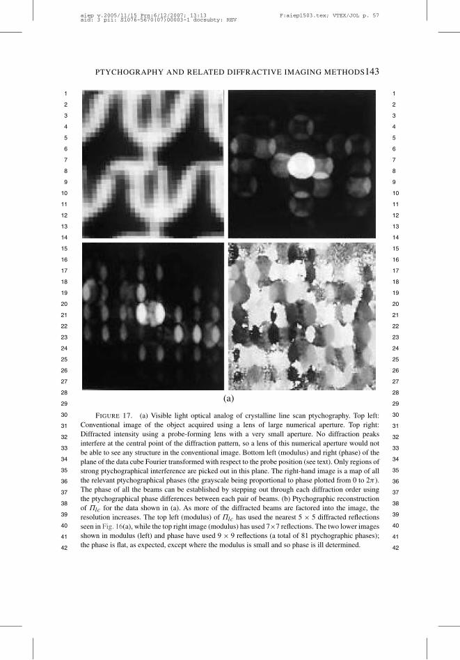
PTYCHOGRAPHY AND RELATED DIFFRACTIVE IMAGING METHODS143
1 1
2 2
3 3
4 4
5 5
6 6
7 7
8 8
9 9
10 10
11 11
12 12
13 13
14 14
15 15
16 16
17 17
18 18
19 19
20 20
21 21
22 22
23 23
24 24
25 25
26 26
27 27
28 28
29 29
30 30
31 31
32 32
33 33
34 34
35 35
36 36
37 37
38 38
39 39
40 40
41 41
42 42
(a)
FIGURE 17. (a) Visible light optical analog of crystalline line scan ptychography. Top left:Conventional image of the object acquired using a lens of large numerical aperture. Top right:Diffracted intensity using a probe-forming lens with a very small aperture. No diffraction peaksinterfere at the central point of the diffraction pattern, so a lens of this numerical aperture would notbe able to see any structure in the conventional image. Bottom left (modulus) and right (phase) of theplane of the data cube Fourier transformed with respect to the probe position (see text). Only regions ofstrong ptychographical interference are picked out in this plane. The right-hand image is a map of allthe relevant ptychographical phases (the grayscale being proportional to phase plotted from 0 to 2" ).The phase of all the beams can be established by stepping out through each diffraction order usingthe ptychographical phase differences between each pair of beams. (b) Ptychographic reconstructionof +lc for the data shown in (a). As more of the diffracted beams are factored into the image, theresolution increases. The top left (modulus) of +lc has used the nearest 5 , 5 diffracted reflectionsseen in Fig. 16(a), while the top right image (modulus) has used 7,7 reflections. The two lower imagesshown in modulus (left) and phase have used 9 , 9 reflections (a total of 81 ptychographic phases);the phase is flat, as expected, except where the modulus is small and so phase is ill determined.
aiep v.2005/11/15 Prn:6/12/2007; 13:13 F:aiep1503.tex; VTEX/JOL p. 57aid: 3 pii: S1076-5670(07)00003-1 docsubty: REV
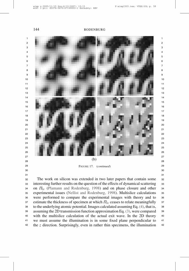
144 RODENBURG
1 1
2 2
3 3
4 4
5 5
6 6
7 7
8 8
9 9
10 10
11 11
12 12
13 13
14 14
15 15
16 16
17 17
18 18
19 19
20 20
21 21
22 22
23 23
24 24
25 25
26 26
27 27
28 28
29 29
30 30
31 31
32 32
33 33
34 34
35 35
36 36
37 37
38 38
39 39
40 40
41 41
42 42
(b)
FIGURE 17. (continued)
The work on silicon was extended in two later papers that contain someinteresting further results on the question of the effects of dynamical scatteringon +lc (Plamann and Rodenburg, 1998) and on phase closure and otherexperimental issues (Nellist and Rodenburg, 1998). Multislice calculationswere performed to compare the experimental images with theory and toestimate the thickness of specimen at which +lc ceases to relate meaningfullyto the underlying atomic potential. Images calculated assuming Eq. (4), that is,assuming the 2D transmission function approximation Eq. (3), were comparedwith the multislice calculation of the actual exit wave. In the 2D theorywe must assume the illumination is in some fixed plane perpendicular tothe z direction. Surprisingly, even in rather thin specimens, the illumination
aiep v.2005/11/15 Prn:6/12/2007; 13:13 F:aiep1503.tex; VTEX/JOL p. 58aid: 3 pii: S1076-5670(07)00003-1 docsubty: REV

PTYCHOGRAPHY AND RELATED DIFFRACTIVE IMAGING METHODS145
1 1
2 2
3 3
4 4
5 5
6 6
7 7
8 8
9 9
10 10
11 11
12 12
13 13
14 14
15 15
16 16
17 17
18 18
19 19
20 20
21 21
22 22
23 23
24 24
25 25
26 26
27 27
28 28
29 29
30 30
31 31
32 32
33 33
34 34
35 35
36 36
37 37
38 38
39 39
40 40
41 41
42 42
defocus does slightly affect the calculated image. With the small range of k-vectors in the incident radiation we would expect changes in the probe as afunction of z to be small. The radius of the aperture used in these experimentsin the back focal plane of the lens was only a little larger than half the angleof the diffraction pattern g-vectors. This means it was too small to formconventional bright-field image fringes at the periodicity of the unit cell. Evena high-resolution conventional image of silicon (where the scattering anglesprocessed by the lens are much larger) produces effectively a projection of theobject; defocusing the lens within the depth of the object produces negligiblechange in the image. It must be remembered, however (Section III.B) that aptychograph integrates a rather larger volume of reciprocal space relative tothe conventional image (Fig. 14). The latter is derived as a result of the lensintegrating the amplitude over a central disk lying on the Ewald sphere.
In fact, the dynamical calculations showed that +lc is remarkably similar tothe real (strongly scattered) exit wave function in silicon provided it is back-propagated to a plane in the center of the object. Figure 18 shows the modulusphase of the calculated exit wave, the modulus and phase of that same waveback-propagated to the mid-plane of the object, and +lc. +lc is independent ofillumination propagation if the relative ptychographical phases are measured
FIGURE 18. Images a and b are the modulus and phase, respectively, of the exit wave calculatedfor [110] silicon with incident energy of 100 keV and sample thickness of 7 nm. This wave is thenback-propagated by 3.5 nm to the plane in the middle of the object (images c and d). The +lc
ptychograph (images e and f) accurately corresponds to this back-propagated wave.
aiep v.2005/11/15 Prn:6/12/2007; 13:13 F:aiep1503.tex; VTEX/JOL p. 59aid: 3 pii: S1076-5670(07)00003-1 docsubty: REV

146 RODENBURG
1 1
2 2
3 3
4 4
5 5
6 6
7 7
8 8
9 9
10 10
11 11
12 12
13 13
14 14
15 15
16 16
17 17
18 18
19 19
20 20
21 21
22 22
23 23
24 24
25 25
26 26
27 27
28 28
29 29
30 30
31 31
32 32
33 33
34 34
35 35
36 36
37 37
38 38
39 39
40 40
41 41
42 42
FIGURE 19. Interfering disks in the STEM electron diffraction pattern. The specimen is siliconoriented onto the [110] zone axis. The fringes result from the parabolic defocus term over the aperturefunction (this pattern was recorded with large defocus in the STEM probe). When recorded in intensity,the defocus phases from adjacent beams contrive to form straight fringes. When the aperture is verylarge, the fringes cross one another and hence build up the shadow image of the periodic object, albeitdominated by coherent effects like in a Gabor hologram.
from exactly the midpoints of the diffracted disk overlaps (provided theprobe-forming optics are symmetric) as first discussed by Spence and Cowley(1978). Figure 19 shows raw data of the diffracted disks from silicon interfer-ing with one another when substantial defocus has been applied to the probe-forming lens: an image that graphically illustrates ptychographic interference.
aiep v.2005/11/15 Prn:6/12/2007; 13:13 F:aiep1503.tex; VTEX/JOL p. 60aid: 3 pii: S1076-5670(07)00003-1 docsubty: REV
PTYCHOGRAPHY AND RELATED DIFFRACTIVE IMAGING METHODS147
1 1
2 2
3 3
4 4
5 5
6 6
7 7
8 8
9 9
10 10
11 11
12 12
13 13
14 14
15 15
16 16
17 17
18 18
19 19
20 20
21 21
22 22
23 23
24 24
25 25
26 26
27 27
28 28
29 29
30 30
31 31
32 32
33 33
34 34
35 35
36 36
37 37
38 38
39 39
40 40
41 41
42 42
Nellist and Rodenburg (1998) measured phase closure between the variousroutes through these diffraction orders (Fig. 20). The very large phase-closureerrors induced by taking triangular routes arise primarily from astigmatismpresent in the lens. A parallelogram route allows such asymmetries to cancelone another and so leads to much smaller phase-closure error. However, evenin the absence of such errors, discrepancies would be expected to arise fromdynamical scattering. Plamann and Rodenburg (1998) calculated these for thesame scattering geometry (Fig. 21). It is noteworthy that for +lc the phase-closure errors are relatively small for thicknesses of silicon less than 10 nm(at 100-keV incident energy) and that low-order reflections (corresponding tolow-resolution information) are reasonably accurate up to 30-nm thickness.(The Bragg–Brentano data set, detailed in the next section, yields much morereliable reconstructions.) In short, even in a fully dynamical model calculationof a crystalline object where all the usual channeling and propagation effectsare strong, the 2D ptychographic approximation does not begin to breakdown until quite substantial specimen thickness. Spence (1978) performedsome similar calculations years ago and reached a similar conclusion: thatthe relative phase between diffracted beams at their midpoint of STEM diskinterference is relative insensitive to dynamical scattering effects. He alsopointed out that as a function of thickness, a phase jump occurs at a thicknessequal to half the extinction distance, in the same way as a contrast reversaloccurs in the bright-field image.
In conclusion, the results of this first experimental demonstration of elec-tron ptychography and the associated dynamical calculations showed threeimportant things. First, although the +lc ptychographic reconstruction doesnot attempt to make any account for the breakdown of 3D geometric andpropagation effects, the resulting image is still a very good estimate of objectstructure seen in projection. In fact, as will be seen in Section IV.B, it ispossible to measure a different subset of I (u,R) that explores rather moreof the 3D information extant in the entire 4D data set. Proper considerationof this may well suggest ways of further accounting for dynamical effectsin order to calculate ptychographs that are even more representative of thescattering potential. Second, perhaps the most significant result from thisproof-of-principle is that the constraints of finite coherence (and hence theso-called information limit) that occur in lens imaging and are generallyacknowledged as the final resolution limit in electron microscopy (even whenundertaken by aberration-corrected lenses) can be overcome by several factorsusing ptychography. Third, although this proof-of-principle was applied to aperiodic and very simple specimen, the same benefits in relation to partialcoherence and dynamical scattering apply to many of the noncrystallinevariants of ptychography. All of these factors bode rather well for the relativeimaging strengths of ptychography.
aiep v.2005/11/15 Prn:6/12/2007; 13:13 F:aiep1503.tex; VTEX/JOL p. 61aid: 3 pii: S1076-5670(07)00003-1 docsubty: REV

148 RODENBURG
1 1
2 2
3 3
4 4
5 5
6 6
7 7
8 8
9 9
10 10
11 11
12 12
13 13
14 14
15 15
16 16
17 17
18 18
19 19
20 20
21 21
22 22
23 23
24 24
25 25
26 26
27 27
28 28
29 29
30 30
31 31
32 32
33 33
34 34
35 35
36 36
37 37
38 38
39 39
40 40
41 41
42 42
(a)
(b)
(c)
(d)
FIGURE 20. Phase closure loops in the experimental silicon +lc . Errors in the triangular routesare large, mostly because of astigmatism in the probe-forming lens. Parallelogram routes use pairsof symmetric interferences (relative to the astigmatism), and hence the phase error cancel. Evenperfect measurements will give phase errors around closure loops because of thickness and dynamicalscattering effects.
aiep v.2005/11/15 Prn:6/12/2007; 13:13 F:aiep1503.tex; VTEX/JOL p. 62aid: 3 pii: S1076-5670(07)00003-1 docsubty: REV
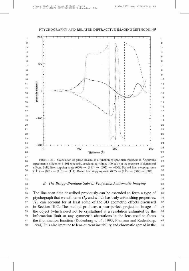
PTYCHOGRAPHY AND RELATED DIFFRACTIVE IMAGING METHODS149
1 1
2 2
3 3
4 4
5 5
6 6
7 7
8 8
9 9
10 10
11 11
12 12
13 13
14 14
15 15
16 16
17 17
18 18
19 19
20 20
21 21
22 22
23 23
24 24
25 25
26 26
27 27
28 28
29 29
30 30
31 31
32 32
33 33
34 34
35 35
36 36
37 37
38 38
39 39
40 40
41 41
42 42
FIGURE 21. Calculation of phase closure as a function of specimen thickness in Ångstroms(specimen is silicon on [110] zone axis, accelerating voltage 100 keV) in the presence of dynamicaleffects. Solid line: stepping route (000) - (111) - (002) - (000). Dashed line: stepping route(111) - (002) - (113) - (111). Dotted line: stepping route (002) - (113) - (004) - (002).
B. The Bragg–Brentano Subset: Projection Achromatic Imaging
The line scan data described previously can be extended to form a type ofptychograph that we will term +p and which has truly astonishing properties.+p can account for at least some of the 3D geometric effects discussedin Section III.C. The method produces a near-perfect projection image ofthe object (which need not be crystalline) at a resolution unlimited by theinformation limit or any symmetric aberrations in the lens used to focusthe illumination function (Rodenburg et al., 1993; Plamann and Rodenburg,1994). It is also immune to lens-current instability and chromatic spread in the
aiep v.2005/11/15 Prn:6/12/2007; 13:13 F:aiep1503.tex; VTEX/JOL p. 63aid: 3 pii: S1076-5670(07)00003-1 docsubty: REV
150 RODENBURG
1 1
2 2
3 3
4 4
5 5
6 6
7 7
8 8
9 9
10 10
11 11
12 12
13 13
14 14
15 15
16 16
17 17
18 18
19 19
20 20
21 21
22 22
23 23
24 24
25 25
26 26
27 27
28 28
29 29
30 30
31 31
32 32
33 33
34 34
35 35
36 36
37 37
38 38
39 39
40 40
41 41
42 42
beam. It is also relatively immune to dynamical scattering and yields a goodrepresentation of the object function even for strong, thick crystals.
The experimental procedure is to scan a 2D array of closely separated real-space illumination positions and then select a particular Fourier componentof the 2D scan at associated detector pixels in the diffraction pattern, each ofwhich corresponds to the Bragg–Brentano diffraction condition for that samereal-space (probe-position) periodicity. Some lengthy explanation is required,but first note that as far as the amount of measured data that are required, thismethod uses the entire 4D data set: NTOTAL = Nu ,Nv ,NX ,NY , where allthe sampling is dense. However, unlike the G- and H -sets that are discussedbelow, we need not undertake entire Fourier transforms (with respect to theillumination position) for every single detector pixel. Instead, we only need asingle Fourier component picked at each detector pixel.
Let the Fourier transform of the 4D intensity data set I (u,R) with respectto the 2D R coordinate be
G(u,U) =!
I (u,R)ei2"R·U dR. (71)
The Bragg–Brentano data set then corresponds to a 2D plane in this 4D datacube given by
B(U) = G
*U
2,U
+. (72)
We can think of this as follows. To form B(U), data are collected in thediffraction plane, each pixel having coordinates given by the 2D vector u. Wecollect diffraction patterns for all the possible (densely sampled) illumination(probe) positions R. Consider a pixel in the detector plane lying at u0. Weform a 2D image as a function of R by observing the intensity that arrives atthis pixel. This is just a conventional image we could call, say, f (R). We takea Fourier transform of this to create a diffractogram, F(U). We then extractfrom F(U) the (complex) value of the single pixel lying at U0 = 2u0 andput this into the array B(U) at the point U0. We do this for all u = u0 andU = 2u0 and thus construct the 2D reciprocal-space function B(U). The backFourier transform of B(U) is the ptychograph +p(R).
The very special properties of B(U) depend on the specimen being reason-ably weakly scattering. (I say “reasonably” because it is still very much anopen question exactly how robust this data set is to dynamical scattering.) Inthe domain of the limited calculations that were performed by Plamann andRodenburg (1998), and the visible light proof-of-principle performed by thesame authors (Plamann and Rodenburg, 1994), it would appear as if +p is
aiep v.2005/11/15 Prn:6/12/2007; 13:13 F:aiep1503.tex; VTEX/JOL p. 64aid: 3 pii: S1076-5670(07)00003-1 docsubty: REV
PTYCHOGRAPHY AND RELATED DIFFRACTIVE IMAGING METHODS151
1 1
2 2
3 3
4 4
5 5
6 6
7 7
8 8
9 9
10 10
11 11
12 12
13 13
14 14
15 15
16 16
17 17
18 18
19 19
20 20
21 21
22 22
23 23
24 24
25 25
26 26
27 27
28 28
29 29
30 30
31 31
32 32
33 33
34 34
35 35
36 36
37 37
38 38
39 39
40 40
41 41
42 42
indeed a very good estimate of the object, even in the presence of quite strongscattering and for thick specimens.
Following the derivation in Rodenburg et al. (1993), we first assume theobject is a 2D transmission weak phase grating of the form
q(r) = 1 " ic/(r), (73a)
where c is a constant and
c''/(r)
'' + 1, (73b)
then the Fourier transform (diffraction pattern) of q(r) is given by
Q(u) = %q(r) = '(u) " icF (u) (74)
where
F(u) = %/(u). (75)
Now according to the fundamental ptychographical Eq. (41)
I (u,R) ='',A(u)ei2"R·u- & Q(u)
''2, (76)
which can be expanded as
I (u,R)
=!!
A(ua)Q(u " ua)A#(ub)Q
#(u " ub)ei2"R·(ua"ub) dua dub,
(77)where ua and ua are dummy variables. Arithmetic manipulations of I (u,R)are key in developing the theory of the entire ptychographical data set.Therefore the required steps in this first example are spelled out in some detail.We use the technique of collapsing integrals via the Dirac delta function; thiscan easily be extended to all the results that are simply stated in later sections.In order to form G(u,U), and hence B(U), we must substitute Eq. (77) intoEq. (71) to derive
G(u,U)
=!!!
A(ua)Q(u " ua)A#(ub)Q
#(u " ub)ei2"R·(ua"ub+U)dua dub dR.
(78)
Note that the integral of ei2"x·u over infinite limits in u is zero unless x iszero. When x is zero, the integral is infinite. Between finite limits – whichwill always occur in a real experiment because the span of the probe positionR and detector range u is finite – the resulting integral as a function of x is
aiep v.2005/11/15 Prn:6/12/2007; 13:13 F:aiep1503.tex; VTEX/JOL p. 65aid: 3 pii: S1076-5670(07)00003-1 docsubty: REV
152 RODENBURG
1 1
2 2
3 3
4 4
5 5
6 6
7 7
8 8
9 9
10 10
11 11
12 12
13 13
14 14
15 15
16 16
17 17
18 18
19 19
20 20
21 21
22 22
23 23
24 24
25 25
26 26
27 27
28 28
29 29
30 30
31 31
32 32
33 33
34 34
35 35
36 36
37 37
38 38
39 39
40 40
41 41
42 42
of the form of sinc(x) in one dimension and has a value of unity. This meansthat in the limit of large limits of integration, sinc(x) has the same propertiesof the Dirac ' function (Eq. (11)). A and Q in the above have no dependenceon R, so we can integrate over it to obtain
G(u,U)
=!!
A(ua)Q(u " ua)A#(ub)Q
#(u " ub)'(ua " ub + U) dua dub.
(79)We can next choose to integrate over either ua or ub. The choice is notessential (but it can reduce the need for subsequent variable substitution). Bythe time coherence functions and 3D scattering considerations are introduced,such integrals can be over many dimensions (e.g., up to 20 in Rodenburg andBates, 1992). Integrating here over ub, the delta function only has value atub = ua + U , so
G(u,U) =!
A(ua)Q(u " ua)A#(ua + U)Q#(u " ua " U) dua. (80)
We then put
uc = u " ua (81)
and reorder to obtain
G(u,U) =!
Q(uc)Q#(uc " U)A#(u " uc + U)A(u " uc) duc. (82)
From Eq. (74)
Q(uc)Q#(uc " U) =
,'(uc) " icF (uc)
-·,'(uc " U) " icF (uc " U)
-#
(83)so
G(u,U) =!
'(uc)'(uc " U)A(u " uc)A#(u " uc + U) duc
" ic
!'(uc " U)F (uc)A(u " uc)A
#(u " uc + U) duc
" ic
!'(uc)F (uc " U)#A(u " uc)A
#(u " uc + U) duc + · · · .(84)
The first integral only has a value when uc = 0 and uc = U . The secondintegral only has value when uc = U ; the third integral only has value when
aiep v.2005/11/15 Prn:6/12/2007; 13:13 F:aiep1503.tex; VTEX/JOL p. 66aid: 3 pii: S1076-5670(07)00003-1 docsubty: REV
PTYCHOGRAPHY AND RELATED DIFFRACTIVE IMAGING METHODS153
1 1
2 2
3 3
4 4
5 5
6 6
7 7
8 8
9 9
10 10
11 11
12 12
13 13
14 14
15 15
16 16
17 17
18 18
19 19
20 20
21 21
22 22
23 23
24 24
25 25
26 26
27 27
28 28
29 29
30 30
31 31
32 32
33 33
34 34
35 35
36 36
37 37
38 38
39 39
40 40
41 41
42 42
uc = 0. We ignore the F 2 term because the object is weak, so now
G(u,U) = '(U)''A(U)
''2
" icF (U)A(u " U)A#(u) " icF #("U)A(u)A#(u + U) + · · · .(85)
Forming B(U) we find
B(U) = '(U)''A(U)
''2 " icF (U)A
*"U
2
+A#
*U
2
+
" icF ("U)A
*U
2
+A#
*3U
2
+. (86a)
Now if the aperture function (the aberration function of the lens) is centrosym-metric, then
A
*"U
2
+= A
*U
2
+, (86b)
and thus whatever the phase of the lens aberrations, the second term inEq. (??) will just be the intensity of the aperture function. If we further assumethat the back focal plane of the probe-forming lens is evenly illuminated withan intensity of radiation |A|2, but has a diaphragm of radius of |U | = (, thenthis second term will have intensity |A|2 provided |U | < 2(, otherwise beingzero. The third term will also have intensity |A|2, but only if |U | < 2(/3;for |U | > 2(/3 the third term is zero. In other words, for the high spatialfrequency region 2( > |U | > 2(/3, we can write simply that
B(U) = |A|2,'(U) " icF (U)
-, (87)
and the back Fourier transform is defined as the ptychograph
+p(r) ) |A|2,1 " ic/(r)
-= |A|2q(r), (88)
the subscript p designating that +p(r) is a projection image of the object(see below). Amazingly, the transmission function of the object has beenreconstructed, scaled by the intensity of the illumination. If fact, we havemade two approximations; we have ignored the second-order F 2 term andthe lower third of the frequency spectrum of the image. However, both ofthese issues arise in conventional imaging, but the conventional image isadditionally subject to all the usual constraints of the form of the particulartransfer function, including its zeros, whereas +p(r) has unity transfer at allspatial frequencies as emphasized by Cowley (2001). Furthermore, its transferfunction is twice the width of the imaging aperture, and in theory this aperture
aiep v.2005/11/15 Prn:6/12/2007; 13:13 F:aiep1503.tex; VTEX/JOL p. 67aid: 3 pii: S1076-5670(07)00003-1 docsubty: REV
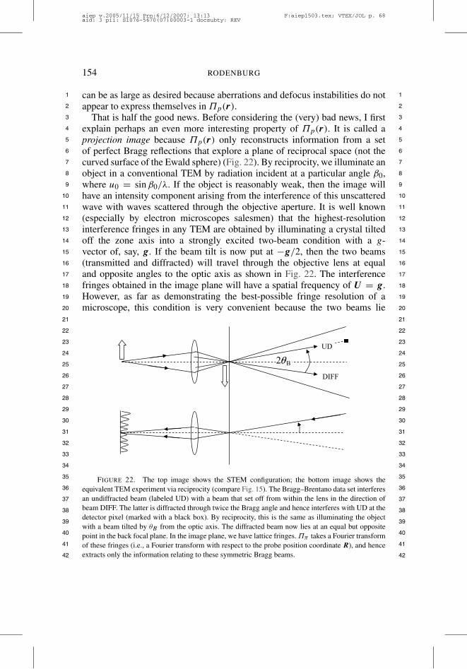
154 RODENBURG
1 1
2 2
3 3
4 4
5 5
6 6
7 7
8 8
9 9
10 10
11 11
12 12
13 13
14 14
15 15
16 16
17 17
18 18
19 19
20 20
21 21
22 22
23 23
24 24
25 25
26 26
27 27
28 28
29 29
30 30
31 31
32 32
33 33
34 34
35 35
36 36
37 37
38 38
39 39
40 40
41 41
42 42
can be as large as desired because aberrations and defocus instabilities do notappear to express themselves in +p(r).
That is half the good news. Before considering the (very) bad news, I firstexplain perhaps an even more interesting property of +p(r). It is called aprojection image because +p(r) only reconstructs information from a setof perfect Bragg reflections that explore a plane of reciprocal space (not thecurved surface of the Ewald sphere) (Fig. 22). By reciprocity, we illuminate anobject in a conventional TEM by radiation incident at a particular angle ,0,where u0 = sin ,0/*. If the object is reasonably weak, then the image willhave an intensity component arising from the interference of this unscatteredwave with waves scattered through the objective aperture. It is well known(especially by electron microscopes salesmen) that the highest-resolutioninterference fringes in any TEM are obtained by illuminating a crystal tiltedoff the zone axis into a strongly excited two-beam condition with a g-vector of, say, g. If the beam tilt is now put at "g/2, then the two beams(transmitted and diffracted) will travel through the objective lens at equaland opposite angles to the optic axis as shown in Fig. 22. The interferencefringes obtained in the image plane will have a spatial frequency of U = g.However, as far as demonstrating the best-possible fringe resolution of amicroscope, this condition is very convenient because the two beams lie
FIGURE 22. The top image shows the STEM configuration; the bottom image shows theequivalent TEM experiment via reciprocity (compare Fig. 15). The Bragg–Brentano data set interferesan undiffracted beam (labeled UD) with a beam that set off from within the lens in the direction ofbeam DIFF. The latter is diffracted through twice the Bragg angle and hence interferes with UD at thedetector pixel (marked with a black box). By reciprocity, this is the same as illuminating the objectwith a beam tilted by -B from the optic axis. The diffracted beam now lies at an equal but oppositepoint in the back focal plane. In the image plane, we have lattice fringes. +" takes a Fourier transformof these fringes (i.e., a Fourier transform with respect to the probe position coordinate R), and henceextracts only the information relating to these symmetric Bragg beams.
aiep v.2005/11/15 Prn:6/12/2007; 13:13 F:aiep1503.tex; VTEX/JOL p. 68aid: 3 pii: S1076-5670(07)00003-1 docsubty: REV
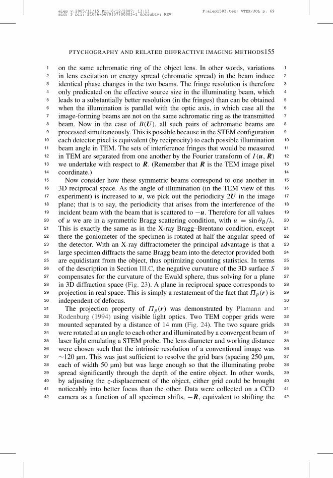
PTYCHOGRAPHY AND RELATED DIFFRACTIVE IMAGING METHODS155
1 1
2 2
3 3
4 4
5 5
6 6
7 7
8 8
9 9
10 10
11 11
12 12
13 13
14 14
15 15
16 16
17 17
18 18
19 19
20 20
21 21
22 22
23 23
24 24
25 25
26 26
27 27
28 28
29 29
30 30
31 31
32 32
33 33
34 34
35 35
36 36
37 37
38 38
39 39
40 40
41 41
42 42
on the same achromatic ring of the object lens. In other words, variationsin lens excitation or energy spread (chromatic spread) in the beam induceidentical phase changes in the two beams. The fringe resolution is thereforeonly predicated on the effective source size in the illuminating beam, whichleads to a substantially better resolution (in the fringes) than can be obtainedwhen the illumination is parallel with the optic axis, in which case all theimage-forming beams are not on the same achromatic ring as the transmittedbeam. Now in the case of B(U), all such pairs of achromatic beams areprocessed simultaneously. This is possible because in the STEM configurationeach detector pixel is equivalent (by reciprocity) to each possible illuminationbeam angle in TEM. The sets of interference fringes that would be measuredin TEM are separated from one another by the Fourier transform of I (u,R)we undertake with respect to R. (Remember that R is the TEM image pixelcoordinate.)
Now consider how these symmetric beams correspond to one another in3D reciprocal space. As the angle of illumination (in the TEM view of thisexperiment) is increased to u, we pick out the periodicity 2U in the imageplane; that is to say, the periodicity that arises from the interference of theincident beam with the beam that is scattered to "u. Therefore for all valuesof u we are in a symmetric Bragg scattering condition, with u = sin -B/*.This is exactly the same as in the X-ray Bragg–Brentano condition, exceptthere the goniometer of the specimen is rotated at half the angular speed ofthe detector. With an X-ray diffractometer the principal advantage is that alarge specimen diffracts the same Bragg beam into the detector provided bothare equidistant from the object, thus optimizing counting statistics. In termsof the description in Section III.C, the negative curvature of the 3D surface Scompensates for the curvature of the Ewald sphere, thus solving for a planein 3D diffraction space (Fig. 23). A plane in reciprocal space corresponds toprojection in real space. This is simply a restatement of the fact that +p(r) isindependent of defocus.
The projection property of +p(r) was demonstrated by Plamann andRodenburg (1994) using visible light optics. Two TEM copper grids weremounted separated by a distance of 14 mm (Fig. 24). The two square gridswere rotated at an angle to each other and illuminated by a convergent beam oflaser light emulating a STEM probe. The lens diameter and working distancewere chosen such that the intrinsic resolution of a conventional image was!120 µm. This was just sufficient to resolve the grid bars (spacing 250 µm,each of width 50 µm) but was large enough so that the illuminating probespread significantly through the depth of the entire object. In other words,by adjusting the z-displacement of the object, either grid could be broughtnoticeably into better focus than the other. Data were collected on a CCDcamera as a function of all specimen shifts, "R, equivalent to shifting the
aiep v.2005/11/15 Prn:6/12/2007; 13:13 F:aiep1503.tex; VTEX/JOL p. 69aid: 3 pii: S1076-5670(07)00003-1 docsubty: REV

156 RODENBURG
1 1
2 2
3 3
4 4
5 5
6 6
7 7
8 8
9 9
10 10
11 11
12 12
13 13
14 14
15 15
16 16
17 17
18 18
19 19
20 20
21 21
22 22
23 23
24 24
25 25
26 26
27 27
28 28
29 29
30 30
31 31
32 32
33 33
34 34
35 35
36 36
37 37
38 38
39 39
40 40
41 41
42 42
FIGURE 23. In the Bragg–Brentano data set, the incident beam is symmetrically tilted relativeto the optic axis with respect to the scattered beam. In this way, we solve for a plane in reciprocalspace, not the amplitude lying over the Ewald sphere as in the conventional image (compare Figs. 12and 14).
FIGURE 24. Schematic of the specimen used to obtain the reconstructions in Fig. 25.
aiep v.2005/11/15 Prn:6/12/2007; 13:13 F:aiep1503.tex; VTEX/JOL p. 70aid: 3 pii: S1076-5670(07)00003-1 docsubty: REV
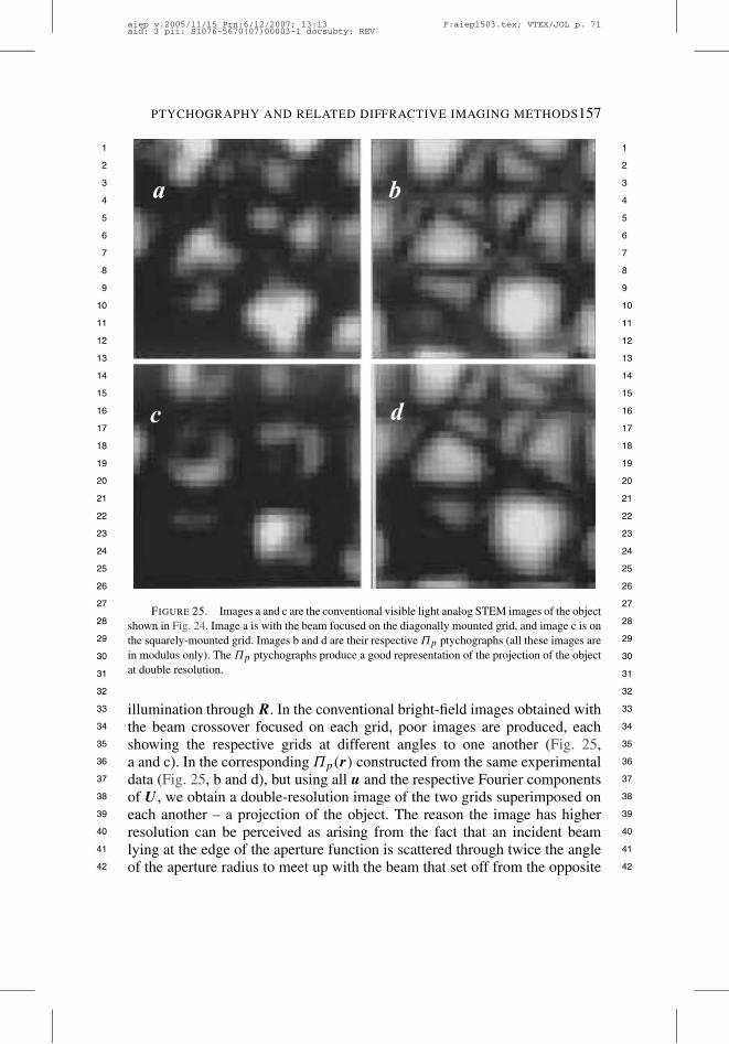
PTYCHOGRAPHY AND RELATED DIFFRACTIVE IMAGING METHODS157
1 1
2 2
3 3
4 4
5 5
6 6
7 7
8 8
9 9
10 10
11 11
12 12
13 13
14 14
15 15
16 16
17 17
18 18
19 19
20 20
21 21
22 22
23 23
24 24
25 25
26 26
27 27
28 28
29 29
30 30
31 31
32 32
33 33
34 34
35 35
36 36
37 37
38 38
39 39
40 40
41 41
42 42
FIGURE 25. Images a and c are the conventional visible light analog STEM images of the objectshown in Fig. 24. Image a is with the beam focused on the diagonally mounted grid, and image c is onthe squarely-mounted grid. Images b and d are their respective +p ptychographs (all these images arein modulus only). The +p ptychographs produce a good representation of the projection of the objectat double resolution.
illumination through R. In the conventional bright-field images obtained withthe beam crossover focused on each grid, poor images are produced, eachshowing the respective grids at different angles to one another (Fig. 25,a and c). In the corresponding +p(r) constructed from the same experimentaldata (Fig. 25, b and d), but using all u and the respective Fourier componentsof U , we obtain a double-resolution image of the two grids superimposed oneach another – a projection of the object. The reason the image has higherresolution can be perceived as arising from the fact that an incident beamlying at the edge of the aperture function is scattered through twice the angleof the aperture radius to meet up with the beam that set off from the opposite
aiep v.2005/11/15 Prn:6/12/2007; 13:13 F:aiep1503.tex; VTEX/JOL p. 71aid: 3 pii: S1076-5670(07)00003-1 docsubty: REV
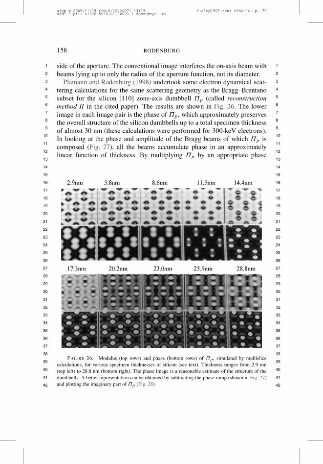
158 RODENBURG
1 1
2 2
3 3
4 4
5 5
6 6
7 7
8 8
9 9
10 10
11 11
12 12
13 13
14 14
15 15
16 16
17 17
18 18
19 19
20 20
21 21
22 22
23 23
24 24
25 25
26 26
27 27
28 28
29 29
30 30
31 31
32 32
33 33
34 34
35 35
36 36
37 37
38 38
39 39
40 40
41 41
42 42
side of the aperture. The conventional image interferes the on-axis beam withbeams lying up to only the radius of the aperture function, not its diameter.
Plamann and Rodenburg (1998) undertook some electron dynamical scat-tering calculations for the same scattering geometry as the Bragg–Brentanosubset for the silicon [110] zone-axis dumbbell +p (called reconstructionmethod II in the cited paper). The results are shown in Fig. 26. The lowerimage in each image pair is the phase of +p, which approximately preservesthe overall structure of the silicon dumbbells up to a total specimen thicknessof almost 30 nm (these calculations were performed for 300-keV electrons).In looking at the phase and amplitude of the Bragg beams of which +p iscomposed (Fig. 27), all the beams accumulate phase in an approximatelylinear function of thickness. By multiplying +p by an appropriate phase
FIGURE 26. Modulus (top rows) and phase (bottom rows) of +p , simulated by multislicecalculations, for various specimen thicknesses of silicon (see text). Thickness ranges from 2.9 nm(top left) to 28.8 nm (bottom right). The phase image is a reasonable estimate of the structure of thedumbbells. A better representation can be obtained by subtracting the phase ramp (shown in Fig. 27)and plotting the imaginary part of +p (Fig. 28).
aiep v.2005/11/15 Prn:6/12/2007; 13:13 F:aiep1503.tex; VTEX/JOL p. 72aid: 3 pii: S1076-5670(07)00003-1 docsubty: REV

PTYCHOGRAPHY AND RELATED DIFFRACTIVE IMAGING METHODS159
1 1
2 2
3 3
4 4
5 5
6 6
7 7
8 8
9 9
10 10
11 11
12 12
13 13
14 14
15 15
16 16
17 17
18 18
19 19
20 20
21 21
22 22
23 23
24 24
25 25
26 26
27 27
28 28
29 29
30 30
31 31
32 32
33 33
34 34
35 35
36 36
37 37
38 38
39 39
40 40
41 41
42 42
offset, the imaginary part of the result is almost a perfect projection of thepotential up to a thickness of !20 nm (Fig. 28).
After enumerating the very beneficial properties of +p, there is somemoderately “bad news.” So far the theory above has ignored the assumptionthat pixels in u and R are infinitesimally small and that the positions andangles spanned by R and u are infinite. If our Fourier transforms are notundertaken over infinite limits, the convenience of the Dirac delta function nolonger applies. This is not intractable, but it must be accounted for by usinga softly varying filter function applied at the experimental limits of the data(McCallum and Rodenburg, 1992). A related problem that severely affects
(a)
FIGURE 27. The modulus (a) and phase (b) of various calculated diffracted beams (see text)as a function of specimen thickness: these are the beams that compose +p . Solid line: (111). Lowestamplitude line is the forbidden reflection (002); in this configuration it remains virtually unexciteduntil a thickness of 20 nm. Other beams shown are (220), (004), and (113). The main inference isthat all the beams acquire a (roughly) linear phase change as a function of thickness. This is why thephase-offset ptychograph (Fig. 28) is more closely representative of the atomic structure.
aiep v.2005/11/15 Prn:6/12/2007; 13:13 F:aiep1503.tex; VTEX/JOL p. 73aid: 3 pii: S1076-5670(07)00003-1 docsubty: REV
160 RODENBURG
1 1
2 2
3 3
4 4
5 5
6 6
7 7
8 8
9 9
10 10
11 11
12 12
13 13
14 14
15 15
16 16
17 17
18 18
19 19
20 20
21 21
22 22
23 23
24 24
25 25
26 26
27 27
28 28
29 29
30 30
31 31
32 32
33 33
34 34
35 35
36 36
37 37
38 38
39 39
40 40
41 41
42 42
(b)
FIGURE 27. (continued)
the experimental feasibility of the method is that these integrals must indeedbe performed over reasonably large fields of view. In other words, a greatdeal of data must be collected before any processing can occur – unlikethe PIE method (the next section), there is no possibility of constructing areal-time image of the object regardless of how much computing power isavailable. If the detector pixels are finite in size – which they must be to getany counts at all – then the aberration insensitivity is lost, at least to firstorder. This is because when the aberrations are large, the intensities fringesin the Ronchigram (the central disk, the shadow image of the probe-formingaperture) are on a very small scale. When a finite pixel integrates over an arealarger than a fringe spacing, the required signal is obliterated. We can picturethis via reciprocity as the illuminating beam in TEM subtending a significantrange of incoherent beams at the specimen plane – an important factor whichaffects the usable information limit. The form of the effective transfer functiongiven these parameters was examined by Nellist and Rodenburg (1994).
aiep v.2005/11/15 Prn:6/12/2007; 13:13 F:aiep1503.tex; VTEX/JOL p. 74aid: 3 pii: S1076-5670(07)00003-1 docsubty: REV
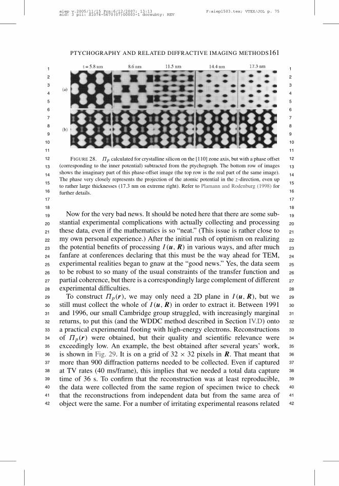
PTYCHOGRAPHY AND RELATED DIFFRACTIVE IMAGING METHODS161
1 1
2 2
3 3
4 4
5 5
6 6
7 7
8 8
9 9
10 10
11 11
12 12
13 13
14 14
15 15
16 16
17 17
18 18
19 19
20 20
21 21
22 22
23 23
24 24
25 25
26 26
27 27
28 28
29 29
30 30
31 31
32 32
33 33
34 34
35 35
36 36
37 37
38 38
39 39
40 40
41 41
42 42
FIGURE 28. +p calculated for crystalline silicon on the [110] zone axis, but with a phase offset(corresponding to the inner potential) subtracted from the ptychograph. The bottom row of imagesshows the imaginary part of this phase-offset image (the top row is the real part of the same image).The phase very closely represents the projection of the atomic potential in the z-direction, even upto rather large thicknesses (17.3 nm on extreme right). Refer to Plamann and Rodenburg (1998) forfurther details.
Now for the very bad news. It should be noted here that there are some sub-stantial experimental complications with actually collecting and processingthese data, even if the mathematics is so “neat.” (This issue is rather close tomy own personal experience.) After the initial rush of optimism on realizingthe potential benefits of processing I (u,R) in various ways, and after muchfanfare at conferences declaring that this must be the way ahead for TEM,experimental realities began to gnaw at the “good news.” Yes, the data seemto be robust to so many of the usual constraints of the transfer function andpartial coherence, but there is a correspondingly large complement of differentexperimental difficulties.
To construct +p(r), we may only need a 2D plane in I (u,R), but westill must collect the whole of I (u,R) in order to extract it. Between 1991and 1996, our small Cambridge group struggled, with increasingly marginalreturns, to put this (and the WDDC method described in Section IV.D) ontoa practical experimental footing with high-energy electrons. Reconstructionsof +p(r) were obtained, but their quality and scientific relevance wereexceedingly low. An example, the best obtained after several years’ work,is shown in Fig. 29. It is on a grid of 32 , 32 pixels in R. That meant thatmore than 900 diffraction patterns needed to be collected. Even if capturedat TV rates (40 ms/frame), this implies that we needed a total data capturetime of 36 s. To confirm that the reconstruction was at least reproducible,the data were collected from the same region of specimen twice to checkthat the reconstructions from independent data but from the same area ofobject were the same. For a number of irritating experimental reasons related
aiep v.2005/11/15 Prn:6/12/2007; 13:13 F:aiep1503.tex; VTEX/JOL p. 75aid: 3 pii: S1076-5670(07)00003-1 docsubty: REV
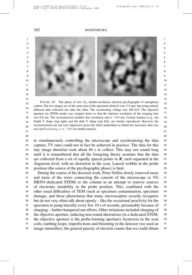
162 RODENBURG
1 1
2 2
3 3
4 4
5 5
6 6
7 7
8 8
9 9
10 10
11 11
12 12
13 13
14 14
15 15
16 16
17 17
18 18
19 19
20 20
21 21
22 22
23 23
24 24
25 25
26 26
27 27
28 28
29 29
30 30
31 31
32 32
33 33
34 34
35 35
36 36
37 37
38 38
39 39
40 40
41 41
42 42
FIGURE 29. The phase of two +p double-resolution electron ptychographs of amorphouscarbon. The two images are of the same area of the specimen (field of view 2.5 nm), but using entirelydifferent data collected one after the other. The accelerating voltage was 100 keV. The objectiveaperture (in STEM mode) was stopped down so that the intrinsic resolution of the imaging lenswas 0.8 nm. The reconstruction doubles this resolution and is !0.4 nm. Certain features (e.g., thebright V shape (top right) and the dark V shape (top left), are clearly reproduced. However, thereconstructions are not very impressive given the effort undertaken to obtain the necessary data (seetext and Rodenburg et al., 1993 for further details).
to simultaneously controlling the microscope and synchronizing the datacapture, TV rates could not in fact be achieved in practice. The data for thistiny image therefore took about 80 s to collect. This may not sound longuntil it is remembered that all the foregoing theory assumes that the dataare collected from a set of equally spaced points in R, each separated at theÅngstrom level, with no distortion in the scan. Lateral wobble in the probeposition (the source of the ptychographic phase) is fatal.
During the course of his doctoral work, Peter Nellist slowly removed moreand more of the wires connecting the console of the microscope (a VGHB501-dedicated STEM) to the column in an attempt to remove sourcesof electronic instability in the probe position. This, combined with theother usual difficulties of TEM (such as specimen contamination, specimendamage, and those phenomena that many microscopists secretly recognizebut do not very often talk about openly – like the occasional proclivity for thespecimen to jump laterally every few 10 s of seconds, presumably because ofcharging – further hampered our efforts. Other irritations included charging ofthe objective aperture, inducing non-round aberrations (in a dedicated STEM,the objective aperture is the probe-forming aperture); hysteresis in the scancoils; earthing loops; imperfections and blooming in the detector (we used animage intensifier); the general paucity of electron counts that we could obtain
aiep v.2005/11/15 Prn:6/12/2007; 13:13 F:aiep1503.tex; VTEX/JOL p. 76aid: 3 pii: S1076-5670(07)00003-1 docsubty: REV
PTYCHOGRAPHY AND RELATED DIFFRACTIVE IMAGING METHODS163
1 1
2 2
3 3
4 4
5 5
6 6
7 7
8 8
9 9
10 10
11 11
12 12
13 13
14 14
15 15
16 16
17 17
18 18
19 19
20 20
21 21
22 22
23 23
24 24
25 25
26 26
27 27
28 28
29 29
30 30
31 31
32 32
33 33
34 34
35 35
36 36
37 37
38 38
39 39
40 40
41 41
42 42
when the source was sufficiently demagnified to achieve an appropriate (evenif rather low) degree of coherence; vibration in the field-emission tip (the VGdesign had the tip mounted on a thin bent wire, which had several vibrationalmodes with which we became all too familiar); and, perhaps worst of all,the need to reduce thermal drift to a usable level of about 1 or 2 Å/min.Even quite simple things, like focusing the probe at the specimen plane,were difficult tasks when the machine was switched to collecting diffractionpatterns. (In short, this was very much a living nightmare, made bearable onlyby the group’s persistent sense of humor.) Cowley and Winterton (2001) dideventually implement the scheme successfully with electrons for a 1D scan ofprobe positions across the edge of a nanotube. Perhaps now that detector anddata transfer/storage technology is so much more advanced, it may be worthrevisiting the technique for 2D objects.
C. Ptychographical Iterative (Pi) Phase-Retrieval Reconstruction
Conventional iterative phase-retrieval methods collect a set of data, whether asingle diffraction pattern from an isolated object, and then process this offline,applying object size constraints in real space. However, as a microscopicimaging method this leaves much to be desired. Microscopists need the abilityto scan their specimens over large fields of view in order to identify areasof interest. Once identified, the user must be able to zoom in to a featureof interest, observing it at higher and higher resolution. Isolated object PDImethods do not allow for this sort of essential microscope functionality.
This sections discusses a recent development in the iterative phase-retrievalmethod that actually owes much more to the ptychographical direct solution:multiple diffraction patterns are recorded as an illumination field is shiftedwith respect to the object of interest (or vice versa). A modified iterativemethod is used to construct the resulting image – a ptychograph that we willcall +" , or a “pi-type” reconstruction. Here we examine in detail a particularvariant of pi-type reconstruction called the PIE algorithm.
Iterative methods of phase retrieval were first proposed by Gerchberg andSaxton (1972) and later developed significantly by Fienup (1978, 1982). Earlywork was performed on 1D objects, if only because of computational con-straints at that time. John Chapman (as differentiated from Henry Chapman,who has also contributed significantly to this field) was the first to consider thepractical issues surrounding an experimental implementation of the techniquein the electron microscope for the 1D image-diffraction plane iterative phase-retrieval (Gerchberg–Saxton) method (Chapman, 1975). The developmentof the personal computer greatly facilitated testing the efficacy of iterativemethods in two dimensions and determining the results of different feedback
aiep v.2005/11/15 Prn:6/12/2007; 13:13 F:aiep1503.tex; VTEX/JOL p. 77aid: 3 pii: S1076-5670(07)00003-1 docsubty: REV

164 RODENBURG
1 1
2 2
3 3
4 4
5 5
6 6
7 7
8 8
9 9
10 10
11 11
12 12
13 13
14 14
15 15
16 16
17 17
18 18
19 19
20 20
21 21
22 22
23 23
24 24
25 25
26 26
27 27
28 28
29 29
30 30
31 31
32 32
33 33
34 34
35 35
36 36
37 37
38 38
39 39
40 40
41 41
42 42
parameters immediately. In two or more dimensions, the method is muchmore robust because of the usual phase problem constraints (discussed inSection II.D). Rather than requiring both image and diffraction intensity data(and hence a good-quality lens, as in the Gerchberg–Saxton algorithm), itwas found (Fienup, 1978) that simply knowing that the object is isolated,effectively embedded in an empty unit cell that has roughly as many (known)zero-valued pixels as pixels in the object image, then the 2D phase problemcan be very effectively solved without significant ambiguity. There are stillstagnation issues resulting from the competition of the inherently ambiguoussolutions (such as q(r) = q#("r), these having the same diffraction patternintensity). Fully complex images are more difficult to solve for (Fienup,1987), but with some refinements, this can sometimes be achieved.
Following a rather stimulating conference organized by Spence et al. (2001)on solution of the nonperiodic phase problem, I was encouraged to revisit theptychographical data set, but with the goal to try to incorporate into it allthe advantages of the iterative technique. The possibility of doing the PDIexperiment in the electron microscope had been discussed as part of a reviewof ptychography (Rodenburg, 1989), but in view of the detector technologyavailable at that time had been dismissed. Using image-plate technology, Zuoet al. (2003) obtained a very impressive reconstruction of a carbon nanotubefrom a single electron diffraction pattern in a single, PDI data set. Giventhat it was possible to achieve an iteratively reconstructed image from asingle diffraction pattern, and given that it is known that it is possible tosolve the phase problem directly from two or more diffraction patterns viaptychography, it seemed logical to suppose that a hybrid method existed thatcould exploit an optimized combination of these methods.
Landauer (1996) had briefly considered processing a number of imagescollected under different illumination conditions in the electron microscopeto reconstruct the modulus and phase of the Fraunhofer diffraction using theknown constraint of the size and shape of the objective aperture lying inthe back focal plane of the object lens. This was far from lenses diffractiveimaging; the work was purely theoretical and had to assume the presenceof a good lens. However, it did indicate that multiple applications of theFienup hybrid input–output method could be “sewn” together to extend theplane of interest (in this case, not the image but the diffraction pattern).Faulkner and Rodenburg (2004) used an aperture constraint alone, presumedto be coincident with the object plane, to show in model calculations thatthe iterative method could indeed be applied to extended real-space objects.Preliminary investigations into the possibility of manufacturing an aperturevia focused ion beam lithography that was small enough to perform this typeof reconstruction in the electron microscope were fraught with difficulties.The aspect ratio of the hole required in order to block off the unwanted
aiep v.2005/11/15 Prn:6/12/2007; 13:13 F:aiep1503.tex; VTEX/JOL p. 78aid: 3 pii: S1076-5670(07)00003-1 docsubty: REV
PTYCHOGRAPHY AND RELATED DIFFRACTIVE IMAGING METHODS165
1 1
2 2
3 3
4 4
5 5
6 6
7 7
8 8
9 9
10 10
11 11
12 12
13 13
14 14
15 15
16 16
17 17
18 18
19 19
20 20
21 21
22 22
23 23
24 24
25 25
26 26
27 27
28 28
29 29
30 30
31 31
32 32
33 33
34 34
35 35
36 36
37 37
38 38
39 39
40 40
41 41
42 42
radiation was large (say a diameter of 10 nm with a depth of 200 nm). Suchapertures contaminate quickly in the microscope and introduce channelingand propagation artifacts.
It became obvious that in any practical implementation of iterative phase-retrieval ptychography, at least in the electron microscope, it would benecessary to use a focused spot of illumination of radiation, as in the STEMconfiguration. Unfortunately, such patches of illumination are necessarily“soft” in the sense that there are always low-amplitude ringing effects thatextend to large distances in the object plane. Because the lens has a limitedextent in reciprocal space, its real-space impulse-response function is alwayssmooth. There are therefore no analogous support-type constraints in realspace. Furthermore, any aberration or defocus in the lens introduces phasechanges into the illuminating beam. A method was required that wouldfeed into the phase-retrieval loop the essence of ptychography: when theillumination function is moved, its shape remains constant; equivalently, thediffraction pattern is a convolution, but a convolution that can be recordedfor a series of phase ramps applied across the Fourier transform of theillumination function, according to the fundamental ptychographical Eq. (41).
The breakthrough came with the development of the so-called PIE updatefunction (Rodenburg and Faulkner, 2004a, 2004b). The use of the measuredmodulus constraint in the Fraunhofer diffraction plane is identical in PIE tothat used in all conventional iterative phase-retrieval methods (Marchesini,2007, provides an excellent review). The difference with PIE that is thereis no simple support constraint in real-space. Instead, a current estimateof the object function is changed incrementally according to the intensityinformation that has been fed in from the diffraction plane.
The iteration proceeds as follows. We seed the algorithm with an initialestimate of +" , which we will call +e,1(r), this being our first (n = 1) suchestimate, labeled (A) in Fig. 30. It is usual to put +e,1(r) = 1; that is, we startby supposing that +e,1(r) is of the form of a transmission grating function ofunity transmission (free space) at all points in r . Suppose we have a currentnth estimate of the ptychograph +e,n(r). Then in the next (n + 1)th iteration,a modified estimate, will be given by +e,n+1(r) according to the equation
+e,n+1(r) = +e,n(r) + U(r)%$c,n(r,Rj ) "
,a(r " Rj ) · +e,n(r)
-&,
(89)where U(r) is an update function, given by
U(r) = |a(r " Rj )||amax(r " Rj )|
a#(r " Rj )
(|a(r " Rj )|2 + 2). (90)
In Eq. (89) we multiply our current estimate of the ptychograph by ourillumination function (which we presume is known accurately) when it is
aiep v.2005/11/15 Prn:6/12/2007; 13:13 F:aiep1503.tex; VTEX/JOL p. 79aid: 3 pii: S1076-5670(07)00003-1 docsubty: REV
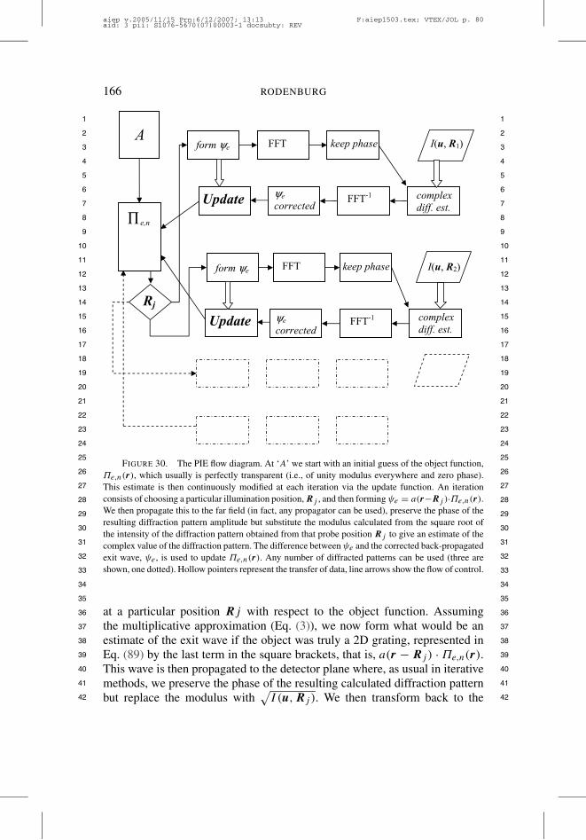
166 RODENBURG
1 1
2 2
3 3
4 4
5 5
6 6
7 7
8 8
9 9
10 10
11 11
12 12
13 13
14 14
15 15
16 16
17 17
18 18
19 19
20 20
21 21
22 22
23 23
24 24
25 25
26 26
27 27
28 28
29 29
30 30
31 31
32 32
33 33
34 34
35 35
36 36
37 37
38 38
39 39
40 40
41 41
42 42
FIGURE 30. The PIE flow diagram. At ‘A’ we start with an initial guess of the object function,+e,n(r), which usually is perfectly transparent (i.e., of unity modulus everywhere and zero phase).This estimate is then continuously modified at each iteration via the update function. An iterationconsists of choosing a particular illumination position, Rj , and then forming $e = a(r"Rj )·+e,n(r).We then propagate this to the far field (in fact, any propagator can be used), preserve the phase of theresulting diffraction pattern amplitude but substitute the modulus calculated from the square root ofthe intensity of the diffraction pattern obtained from that probe position Rj to give an estimate of thecomplex value of the diffraction pattern. The difference between $e and the corrected back-propagatedexit wave, $e , is used to update +e,n(r). Any number of diffracted patterns can be used (three areshown, one dotted). Hollow pointers represent the transfer of data, line arrows show the flow of control.
at a particular position Rj with respect to the object function. Assumingthe multiplicative approximation (Eq. (3)), we now form what would be anestimate of the exit wave if the object was truly a 2D grating, represented inEq. (89) by the last term in the square brackets, that is, a(r " Rj ) · +e,n(r).This wave is then propagated to the detector plane where, as usual in iterativemethods, we preserve the phase of the resulting calculated diffraction patternbut replace the modulus with
/I (u,Rj ). We then transform back to the
aiep v.2005/11/15 Prn:6/12/2007; 13:13 F:aiep1503.tex; VTEX/JOL p. 80aid: 3 pii: S1076-5670(07)00003-1 docsubty: REV
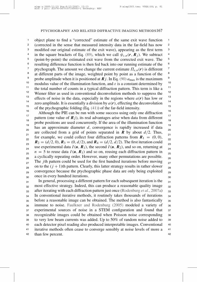
PTYCHOGRAPHY AND RELATED DIFFRACTIVE IMAGING METHODS167
1 1
2 2
3 3
4 4
5 5
6 6
7 7
8 8
9 9
10 10
11 11
12 12
13 13
14 14
15 15
16 16
17 17
18 18
19 19
20 20
21 21
22 22
23 23
24 24
25 25
26 26
27 27
28 28
29 29
30 30
31 31
32 32
33 33
34 34
35 35
36 36
37 37
38 38
39 39
40 40
41 41
42 42
object plane to find a “corrected” estimate of the same exit wave function(corrected in the sense that measured intensity data in the far-field has nowmodified our original estimate of the exit wave), appearing as the first termin the square brackets of Eq. (89), which we call $c,n(r,Rj ). We subtract(point-by-point) the estimated exit wave from the corrected exit wave. Theresulting difference function is then fed back into our running estimate of theptychograph. The amount we change the current estimate +e,n(r) is differentat different parts of the image, weighted point by point as a function of theprobe amplitude when it is positioned at Rj . In Eq. (90) amax is the maximummodulus value of the illumination function, and 2 is a constant determined bythe total number of counts in a typical diffraction pattern. This term is like aWiener filter as used in conventional deconvolution methods to suppress theeffects of noise in the data, especially in the regions where a(r) has low orzero amplitude. It is essentially a division by a(r), effecting the deconvolutionof the ptychographic folding (Eq. (41)) of the far-field intensity.
Although the PIE can be run with some success using only one diffractionpattern (one value of Rj ), its real advantages arise when data from differentprobe positions are used concurrently. If the area of the illumination functionhas an approximate diameter d , convergence is rapidly increased if dataare collected from a grid of points separated in R by about d/2. Thus,for example, we could collect four diffraction patterns from R1 = (0, 0),R2 = (d/2, 0), R3 = (0, d/2), and R4 = (d/2, d/2). The first iteration coulduse experimental data I (u,R1), the second I (u,R2), and so on, returning atn = 5 to reuse data I (u,R1) and so on, reusing each diffraction pattern ina cyclically repeating order. However, many other permutations are possible.The j th pattern could be used for the first hundred iterations before movingon to the (j + 1)th pattern. Clearly, this latter strategy results in rather slowerconvergence because the ptychographic phase data are only being exploitedonce in every hundred iterations.
In general, processing a different pattern for each subsequent iteration is themost effective strategy. Indeed, this can produce a reasonable quality imageafter iterating with each diffraction pattern just once (Rodenburg et al., 2007a)In conventional iterative methods, it routinely takes thousands of iterationsbefore a reasonable image can be obtained. The method is also fantasticallyimmune to noise. Faulkner and Rodenburg (2005) modeled a variety ofexperimental sources of noise in a STEM configuration and found thatrecognizable images could be obtained when Poisson noise correspondingto very low beam currents was added. Up to 50% of random noise added toeach detector pixel reading also produced interpretable images. Conventionaliterative methods often cease to converge sensibly at noise levels of more athan few percent.
aiep v.2005/11/15 Prn:6/12/2007; 13:13 F:aiep1503.tex; VTEX/JOL p. 81aid: 3 pii: S1076-5670(07)00003-1 docsubty: REV

168 RODENBURG
1 1
2 2
3 3
4 4
5 5
6 6
7 7
8 8
9 9
10 10
11 11
12 12
13 13
14 14
15 15
16 16
17 17
18 18
19 19
20 20
21 21
22 22
23 23
24 24
25 25
26 26
27 27
28 28
29 29
30 30
31 31
32 32
33 33
34 34
35 35
36 36
37 37
38 38
39 39
40 40
41 41
42 42
It should be remembered that the data collection process is completelydecoupled from the iterative calculation itself. The reconstruction can beprocessed offline, after all the data have been collected, or in real time,concurrently as further data are being collected. Because the PIE is completelyindifferent to the position of the next Rj , the field of view can extendedcontinuously, in real time, according to whatever part of the specimen theuser wishes to image. This is one of the defining properties of PIE. Thefield of view is independent of the size of the detector. Clearly, the samplingcondition must still be satisfied, but this depends only on the width of theillumination function – it is nothing to do with the size of the final field ofview. The forward and back propagations necessary for each iteration can beconducted on a reciprocal space sampling of say, &us , which defines a valueof d ) 2/&us . However, any particular value of Rj is unconstrained by d . Wecould use data from R1 = (100d, 50d) and R2 = ((100 · 5)d, (50 · 5)d) anduse the update function to alter only the area of ptychograph spanned by theillumination function when it is centered on either of these coordinates. Thereis nothing to stop +" spanning a total image area of, say, 1000,1000d2. If thedetector has 1000 ,1000 pixels, then in this situation the entire ptychographcould contain 106 ,106 pixels: unlike conventional iterative methods, the sizeof the reconstruction can be as large as desired.
Figure 31 shows a visible light experimental demonstration of the PIEmethod (from Rodenburg et al., 2007a). The illumination function wasgenerated simply by an aperture somewhat upstream of the object (a 3-mmlong ant sectioned and mounted between a microscope slide and cover slip).The aperture was 0.8 mm in diameter, with * = 630 nm. The object wasmoved over a grid of 10,10 illumination positions, each separated by slightlyless than half the aperture width. An example of a typical diffraction patternis shown in Fig. 32, as is the recorded intensity of the illumination function atthe plane where it impinges on the object. As can be seen, the disc of the real-space aperture has been blurred out by propagation, causing Fresnel fringe-like features to develop around the edges of it. This function is therefore “soft”and does not present us with the sort of sharp support function required forconventional iterative phase retrieval. Figure 31 shows intensity and phasereconstructions of +" . The resolution of the ptychrograph is !17 µm; that is,about 50 times smaller than the diameter of the aperture.
Note that in the phase of the reconstruction we can discern a phase rampacross the entire image. This is due to the cover slip not being perfectlyparallel to the underlying slide. More recent unpublished work has shownslowly changing phase distribution over very wide fields of view can beaccurately reconstructed. The same sort of information can be extracted fromholograms, but here we do not have any interferometric optical component
aiep v.2005/11/15 Prn:6/12/2007; 13:13 F:aiep1503.tex; VTEX/JOL p. 82aid: 3 pii: S1076-5670(07)00003-1 docsubty: REV

PTYCHOGRAPHY AND RELATED DIFFRACTIVE IMAGING METHODS169
1 1
2 2
3 3
4 4
5 5
6 6
7 7
8 8
9 9
10 10
11 11
12 12
13 13
14 14
15 15
16 16
17 17
18 18
19 19
20 20
21 21
22 22
23 23
24 24
25 25
26 26
27 27
28 28
29 29
30 30
31 31
32 32
33 33
34 34
35 35
36 36
37 37
38 38
39 39
40 40
41 41
42 42
FIGURE 31. Visible light +" reconstruction (i.e., +e,n, where in this case n = 25). Residualstructure in the modulus (left) arises from slight detector misalignment and misestimate of theillumination function: the 10 , 10 scan of probe positions is hence visible. Note that in the phaseimage (right), a slowly varying phase ramp is discernible – such large-scale phase variations (in thiscase due to a curved cover slip) are lost in conventional Zernike and electron microscopic images. Theant is !3 mm in length, the scale bar is 1 mm. For more details, see Rodenburg et al. (2007a).
FIGURE 32. Raw data of ant reconstruction shown in Fig. 31. The intensity of the illuminationfunction (left) is measured at the plane of the object. Note that propagation between the aperture andthe object has led to the development of Fresnel fringes around its edges. A typical diffraction patternis shown on the right.
or lens, except the diffraction itself occurring at the object plane. This is apotentially important imaging capability of pi-type ptychography.
A much more scientifically significant result is shown in Fig. 33 (from Ro-denburg et al., 2007b) where an exactly analogous experimental configuration
aiep v.2005/11/15 Prn:6/12/2007; 13:13 F:aiep1503.tex; VTEX/JOL p. 83aid: 3 pii: S1076-5670(07)00003-1 docsubty: REV
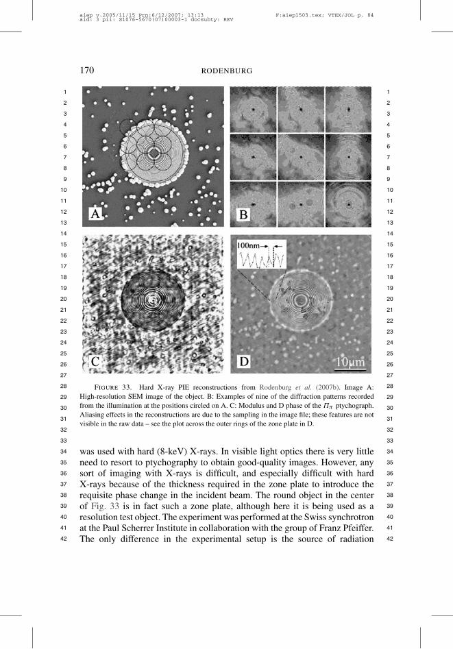
170 RODENBURG
1 1
2 2
3 3
4 4
5 5
6 6
7 7
8 8
9 9
10 10
11 11
12 12
13 13
14 14
15 15
16 16
17 17
18 18
19 19
20 20
21 21
22 22
23 23
24 24
25 25
26 26
27 27
28 28
29 29
30 30
31 31
32 32
33 33
34 34
35 35
36 36
37 37
38 38
39 39
40 40
41 41
42 42
FIGURE 33. Hard X-ray PIE reconstructions from Rodenburg et al. (2007b). Image A:High-resolution SEM image of the object. B: Examples of nine of the diffraction patterns recordedfrom the illumination at the positions circled on A. C: Modulus and D phase of the +" ptychograph.Aliasing effects in the reconstructions are due to the sampling in the image file; these features are notvisible in the raw data – see the plot across the outer rings of the zone plate in D.
was used with hard (8-keV) X-rays. In visible light optics there is very littleneed to resort to ptychography to obtain good-quality images. However, anysort of imaging with X-rays is difficult, and especially difficult with hardX-rays because of the thickness required in the zone plate to introduce therequisite phase change in the incident beam. The round object in the centerof Fig. 33 is in fact such a zone plate, although here it is being used as aresolution test object. The experiment was performed at the Swiss synchrotronat the Paul Scherrer Institute in collaboration with the group of Franz Pfeiffer.The only difference in the experimental setup is the source of radiation
aiep v.2005/11/15 Prn:6/12/2007; 13:13 F:aiep1503.tex; VTEX/JOL p. 84aid: 3 pii: S1076-5670(07)00003-1 docsubty: REV
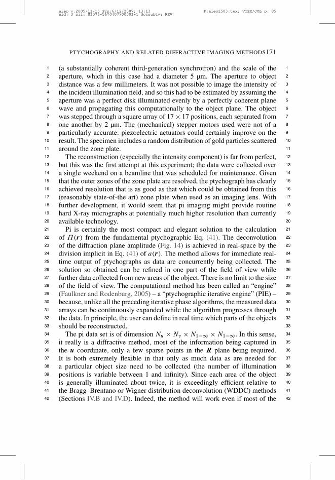
PTYCHOGRAPHY AND RELATED DIFFRACTIVE IMAGING METHODS171
1 1
2 2
3 3
4 4
5 5
6 6
7 7
8 8
9 9
10 10
11 11
12 12
13 13
14 14
15 15
16 16
17 17
18 18
19 19
20 20
21 21
22 22
23 23
24 24
25 25
26 26
27 27
28 28
29 29
30 30
31 31
32 32
33 33
34 34
35 35
36 36
37 37
38 38
39 39
40 40
41 41
42 42
(a substantially coherent third-generation synchrotron) and the scale of theaperture, which in this case had a diameter 5 µm. The aperture to objectdistance was a few millimeters. It was not possible to image the intensity ofthe incident illumination field, and so this had to be estimated by assuming theaperture was a perfect disk illuminated evenly by a perfectly coherent planewave and propagating this computationally to the object plane. The objectwas stepped through a square array of 17 , 17 positions, each separated fromone another by 2 µm. The (mechanical) stepper motors used were not of aparticularly accurate: piezoelectric actuators could certainly improve on theresult. The specimen includes a random distribution of gold particles scatteredaround the zone plate.
The reconstruction (especially the intensity component) is far from perfect,but this was the first attempt at this experiment; the data were collected overa single weekend on a beamline that was scheduled for maintenance. Giventhat the outer zones of the zone plate are resolved, the ptychograph has clearlyachieved resolution that is as good as that which could be obtained from this(reasonably state-of-the art) zone plate when used as an imaging lens. Withfurther development, it would seem that pi imaging might provide routinehard X-ray micrographs at potentially much higher resolution than currentlyavailable technology.
Pi is certainly the most compact and elegant solution to the calculationof +(r) from the fundamental ptychographic Eq. (41). The deconvolutionof the diffraction plane amplitude (Fig. 14) is achieved in real-space by thedivision implicit in Eq. (41) of a(r). The method allows for immediate real-time output of ptychographs as data are concurrently being collected. Thesolution so obtained can be refined in one part of the field of view whilefurther data collected from new areas of the object. There is no limit to the sizeof the field of view. The computational method has been called an “engine”(Faulkner and Rodenburg, 2005) – a “ptychographic iterative engine” (PIE) –because, unlike all the preceding iterative phase algorithms, the measured dataarrays can be continuously expanded while the algorithm progresses throughthe data. In principle, the user can define in real time which parts of the objectsshould be reconstructed.
The pi data set is of dimension Nu , Nv , N1"( , N1"(. In this sense,it really is a diffractive method, most of the information being captured inthe u coordinate, only a few sparse points in the R plane being required.It is both extremely flexible in that only as much data as are needed fora particular object size need to be collected (the number of illuminationpositions is variable between 1 and infinity). Since each area of the objectis generally illuminated about twice, it is exceedingly efficient relative tothe Bragg–Brentano or Wigner distribution deconvolution (WDDC) methods(Sections IV.B and IV.D). Indeed, the method will work even if most of the
aiep v.2005/11/15 Prn:6/12/2007; 13:13 F:aiep1503.tex; VTEX/JOL p. 85aid: 3 pii: S1076-5670(07)00003-1 docsubty: REV

172 RODENBURG
1 1
2 2
3 3
4 4
5 5
6 6
7 7
8 8
9 9
10 10
11 11
12 12
13 13
14 14
15 15
16 16
17 17
18 18
19 19
20 20
21 21
22 22
23 23
24 24
25 25
26 26
27 27
28 28
29 29
30 30
31 31
32 32
33 33
34 34
35 35
36 36
37 37
38 38
39 39
40 40
41 41
42 42
object is only illuminated once, although increased redundancy helps with theconvergence of the algorithm.
D. The Wigner Distribution Deconvolution Method
In Section IV.B we formed a function G(u,U), calculated by taking theFourier transform of I (u,R) with respect to the R coordinate. From thiswe could extract B(U) and hence the projection pytochograph. However,B(U) is just a 2D subset of an intrinsically 4D data set. By picking onlyone particular Fourier component in U for each location in u, a huge amountof data are wasted. In fact, the Bragg–Brentano subset was only developedmuch later as a result of a different line of reasoning that had been sparkedin the autumn of 1988 when Owen Saxton very helpfully introduced me toProfessor Richard Bates, who was passing through Cambridge on his wayfrom New Zealand to a conference in Europe. Our meeting only lasted 20minutes and was mostly spent brewing and drinking tea. Richard was severelyjet lagged. His long white hair was characteristically disheveled; he struck meas the archetypal mad professor. I had an imminent teaching commitment thatafternoon and so had to bring the social niceties to an abrupt end. In the lasttwo minutes before racing off, I scribbled down Eq. (41) and said that I wouldbe very grateful to receive any suggestions on how to obtain a comprehensivesolution for the object function q(r), given only the intensity I (u,R) anda knowledge of a(r). I did not hear from him at all until I received a telex6 months later: it said, “I have solved your problem. Please send fax number.”The stream of equations that subsequently came out of the fax machine atfirst completely confused me. A day or two later I was first enlightened andthen delighted. Two weeks later I was frantically writing a research grantproposal. Without that telex, this Chapter, and most of what is in it, would notexist. The brief collaboration that followed was truly fruitful. I was a cynicalexperimentalist; Richard was an inspired theoretician who passionately lovedthe phase problem and had worked on it for many years from a wide range ofperspectives. I could relate many stories at this point: sometimes sparks wouldfly; Richard was a true original but also, at times, incredibly stubborn. He diedof cancer 2 years after our first meeting, just as a vast horizon of future workwas expanding before us. I was impressed that he remained absolutely focusedon productive work right until the very end, never at any point being aggrievedthat fate had determined that he would die much younger than today’s averagespan.
What he wrote in that fax (disguised somewhat in his inimitable nomencla-ture and penchant for massive equations) was that if
H(U , r) =!!
I (u,R)ei2"(R·r"u·U) du dR, (91)
aiep v.2005/11/15 Prn:6/12/2007; 13:13 F:aiep1503.tex; VTEX/JOL p. 86aid: 3 pii: S1076-5670(07)00003-1 docsubty: REV
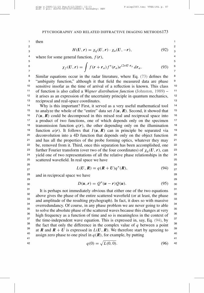
PTYCHOGRAPHY AND RELATED DIFFRACTIVE IMAGING METHODS173
1 1
2 2
3 3
4 4
5 5
6 6
7 7
8 8
9 9
10 10
11 11
12 12
13 13
14 14
15 15
16 16
17 17
18 18
19 19
20 20
21 21
22 22
23 23
24 24
25 25
26 26
27 27
28 28
29 29
30 30
31 31
32 32
33 33
34 34
35 35
36 36
37 37
38 38
39 39
40 40
41 41
42 42
then
H(U , r) = 3q(U , r) · 3a(U ,"r), (92)
where for some general function, f (r),
3f (U , r) =!
f (r + ra)f#(ra)e
i2"U ·ra dra. (93)
Similar equations occur in the radar literature, where Eq. (73) defines the“ambiguity function,” although it that field the measured data are phasesensitive insofar as the time of arrival of a reflection is known. This classof function is also called a Wigner distribution function (Johnston, 1989) –it arises as an expression of the uncertainty principle in quantum mechanics,reciprocal and real-space coordinates.
Why is this important? First, it served as a very useful mathematical toolto analyze the whole of the “entire” data set I (u,R). Second, it showed thatI (u,R) could be decomposed in this mixed real and reciprocal space intoa product of two functions, one of which depends only on the specimentransmission function q(r), the other depending only on the illuminationfunction a(r). It follows that I (u,R) can in principle be separated viadeconvolution into a 4D function that depends only on the object functionand has all the properties of the probe forming optics, whatever they maybe, removed from it. Third, once this separation has been accomplished, onefurther Fourier transform (over two of the four coordinates) of 3q(U , r), canyield one of two representations of all the relative phase relationships in thescattered wavefield. In real space we have
L(U ,R) = q(R + U)q#(R), (94)
and in reciprocal space we have
D(u, r) = Q#(u " r)Q(u). (95)
It is perhaps not immediately obvious that either one of the two equationsabove gives the phase of the entire scattered wavefield (or at least, the phaseand amplitude of the resulting ptychograph). In fact, it does so with massiveoverredundancy. Of course, in any phase problem we are never going to ableto solve the absolute phase of the scattered waves because this changes at veryhigh frequency as a function of time and so is meaningless in the context ofthe time-independent wave equation. This is expressed in, say, Eq. (94), bythe fact that only the difference in the complex value of q between a pointat R and R + U is expressed in L(U ,R). We therefore start by agreeing toassign zero phase to one pixel in q(R), for example, by putting
q(0) =/
L(0, 0). (96)
aiep v.2005/11/15 Prn:6/12/2007; 13:13 F:aiep1503.tex; VTEX/JOL p. 87aid: 3 pii: S1076-5670(07)00003-1 docsubty: REV

174 RODENBURG
1 1
2 2
3 3
4 4
5 5
6 6
7 7
8 8
9 9
10 10
11 11
12 12
13 13
14 14
15 15
16 16
17 17
18 18
19 19
20 20
21 21
22 22
23 23
24 24
25 25
26 26
27 27
28 28
29 29
30 30
31 31
32 32
33 33
34 34
35 35
36 36
37 37
38 38
39 39
40 40
41 41
42 42
The WDDC ptychograph is then given by
+W(U) = L(U , 0).L(0, 0)
. (97)
However, we can choose to assign any phase to any pixel in q(R), and form adifferent ptychograph by dividing L(U ,R) by that pixel. In other words, wecan form a whole family of ptychographs
+W(U ,RU) = L(U ,Ru)
|.L(0,Ru)|. (98)
It was quickly discovered (Rodenburg, 1989) that though the WDDC could bemade relatively immune to noise by performing the deconvolution step usinga Wiener filter, fatal errors arose when the illumination function was “soft” inbeing bandwidth limited in the sense that there is a sharp aperture in the backfocal plane (e.g., as in the case when a(r) is of the form of a STEM probegenerated by a lens with a diaphragm). This is akin to the difficulties that arisein iterative phase retrieval in the same configuration when there is no definiteand sharp support function in the object plane. The calculation presented inBates and Rodenburg (1989) had to be performed using a truncated probe (i.e.,a finite probe cut off with a sharp edge) in order to make the method work atall. Although this was alluded to in the last paragraph in Section 3 of thatpaper, it was of great concern to the author. Clearly, if a sharp-edged featureis a requirement of the method, then it is also true that a lens of very widenumerical aperture is required, defeating the whole purpose of ptychography.
The reciprocal version of the method (Eq. (96)) was found much later toovercome this latter difficulty (Rodenburg and Bates, 1992). In reciprocalspace, the aperture function is sharp, and so its Fourier transform has valueout to very large values of u, meaning that the deconvolution step does notencounter divide-by-zeros except at a few points; these can be avoided byusing other volumes of the data set (which is extremely redundant). Onceagain, we can construct a whole family of ptychographs. The fact that theaperture is finite may seem to imply that one such ptychograph, for example
%,+W("r)
-= D#(0, r).
D(0, 0)(99)
would be limited in r , and hence there would be no gain in resolution. Butthis is not the case. We use the term stepping out (see Section IV.A andFig. 17(a)) to suggest that even if D(u, r) is of limited extent in r , we canuse the phase reconstructed from one plane, say from D(0, r), to obtain anestimate of %(+W(r)) up to the aperture diameter 2(. Once we have the phaseat %(+W(2()), we now use a new plane of D(u, r), namely, D(2(, r), to
aiep v.2005/11/15 Prn:6/12/2007; 13:13 F:aiep1503.tex; VTEX/JOL p. 88aid: 3 pii: S1076-5670(07)00003-1 docsubty: REV
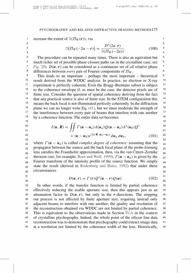
PTYCHOGRAPHY AND RELATED DIFFRACTIVE IMAGING METHODS175
1 1
2 2
3 3
4 4
5 5
6 6
7 7
8 8
9 9
10 10
11 11
12 12
13 13
14 14
15 15
16 16
17 17
18 18
19 19
20 20
21 21
22 22
23 23
24 24
25 25
26 26
27 27
28 28
29 29
30 30
31 31
32 32
33 33
34 34
35 35
36 36
37 37
38 38
39 39
40 40
41 41
42 42
increase the extent of %(+W(r)), via
%,+W("2( " r)
-= D#(2(, r)
%(+W("2()). (100)
The procedure can be repeated many times. There is also an equivalent butmuch richer set of possible phase-closure paths (as in the crystalline case; seeFig. 20). D(u, r) can be considered as a continuous set of all relative phasedifferences between every pair of Fourier components of +W .
This leads to an important – perhaps the most important – theoreticalresult derived from the WDDC analysis. In practice, no electron or X-rayexperiment is perfectly coherent. Even the Bragg–Brentano subset is subjectto the coherence envelope if, as must be the case, the detector pixels are offinite size. Consider the question of spatial coherence deriving from the factthat any practical source is also of finite size. In the STEM configuration thismeans the back focal is not illuminated perfectly coherently. In the diffractionplane we can no longer write Eq. (41), but we must moderate the strength ofthe interference between every pair of beams that interfere with one anotherby a coherence function. The entire data set becomes
I (u,R) =!!
4 (u " ua)A(ua)Q(u " ua)A#(ub)Q
#
, (u " ub)ei2"R·(ua"ub) dua dub, (101)
where 4 (u " ua) is called complex degree of coherence: assuming that thepropagator between the source and the back focal plane of the probe-forminglens satisfies the Fraunhofer approximation, then, via the van Cittert–Zerniketheorem (see, for example, Born and Wolf, 1999), 4 (u " ua) is given by theFourier transform of the intensity profile of the source function. We simplystate the result (derived in Rodenburg and Bates, 1992) that under thesecircumstances
D(u, r) = 4 (r)Q#(u " r)Q(u). (102)
In other words, if the transfer function is limited by partial coherenceeffectively reducing the usable aperture size, then this appears just as anattenuation factor in D(u, r), but only in the r-directions. The steppingout process is not affected by finite aperture size, requiring instead onlyadjacent beams to interfere with one another; the quality and resolution ofthe reconstruction obtained via WDDC are not limited by partial coherence.This is equivalent to the observations made in Section IV.A in the contextof crystalline ptychography. Indeed, the whole point of the silicon line-datareconstruction was to demonstrate that ptychography could extract image dataat a resolution not limited by the coherence width of the lens. Historically,
aiep v.2005/11/15 Prn:6/12/2007; 13:13 F:aiep1503.tex; VTEX/JOL p. 89aid: 3 pii: S1076-5670(07)00003-1 docsubty: REV
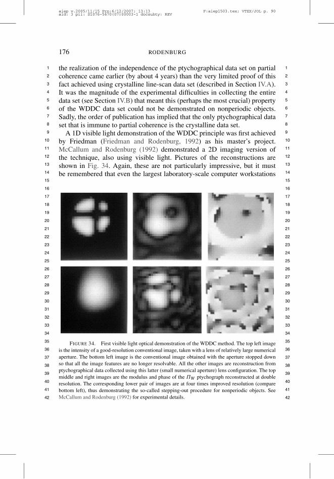
176 RODENBURG
1 1
2 2
3 3
4 4
5 5
6 6
7 7
8 8
9 9
10 10
11 11
12 12
13 13
14 14
15 15
16 16
17 17
18 18
19 19
20 20
21 21
22 22
23 23
24 24
25 25
26 26
27 27
28 28
29 29
30 30
31 31
32 32
33 33
34 34
35 35
36 36
37 37
38 38
39 39
40 40
41 41
42 42
the realization of the independence of the ptychographical data set on partialcoherence came earlier (by about 4 years) than the very limited proof of thisfact achieved using crystalline line-scan data set (described in Section IV.A).It was the magnitude of the experimental difficulties in collecting the entiredata set (see Section IV.B) that meant this (perhaps the most crucial) propertyof the WDDC data set could not be demonstrated on nonperiodic objects.Sadly, the order of publication has implied that the only ptychographical dataset that is immune to partial coherence is the crystalline data set.
A 1D visible light demonstration of the WDDC principle was first achievedby Friedman (Friedman and Rodenburg, 1992) as his master’s project.McCallum and Rodenburg (1992) demonstrated a 2D imaging version ofthe technique, also using visible light. Pictures of the reconstructions areshown in Fig. 34. Again, these are not particularly impressive, but it mustbe remembered that even the largest laboratory-scale computer workstations
FIGURE 34. First visible light optical demonstration of the WDDC method. The top left imageis the intensity of a good-resolution conventional image, taken with a lens of relatively large numericalaperture. The bottom left image is the conventional image obtained with the aperture stopped downso that all the image features are no longer resolvable. All the other images are reconstruction fromptychographical data collected using this latter (small numerical aperture) lens configuration. The topmiddle and right images are the modulus and phase of the +W ptychograph reconstructed at doubleresolution. The corresponding lower pair of images are at four times improved resolution (comparebottom left), thus demonstrating the so-called stepping-out procedure for nonperiodic objects. SeeMcCallum and Rodenburg (1992) for experimental details.
aiep v.2005/11/15 Prn:6/12/2007; 13:13 F:aiep1503.tex; VTEX/JOL p. 90aid: 3 pii: S1076-5670(07)00003-1 docsubty: REV
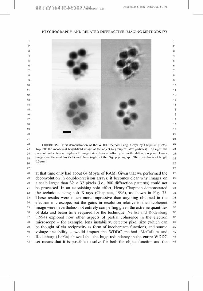
PTYCHOGRAPHY AND RELATED DIFFRACTIVE IMAGING METHODS177
1 1
2 2
3 3
4 4
5 5
6 6
7 7
8 8
9 9
10 10
11 11
12 12
13 13
14 14
15 15
16 16
17 17
18 18
19 19
20 20
21 21
22 22
23 23
24 24
25 25
26 26
27 27
28 28
29 29
30 30
31 31
32 32
33 33
34 34
35 35
36 36
37 37
38 38
39 39
40 40
41 41
42 42
FIGURE 35. First demonstration of the WDDC method using X-rays by Chapman (1996).Top left: the incoherent bright-field image of the object (a group of latex particles). Top right: theconventional coherent bright-field image taken from an offset pixel in the diffraction plane. Lowerimages are the modulus (left) and phase (right) of the +W ptychograph. The scale bar is of length0.5 µm.
at that time only had about 64 Mbyte of RAM. Given that we performed thedeconvolution in double-precision arrays, it becomes clear why images ona scale larger than 32 , 32 pixels (i.e., 900 diffraction patterns) could notbe processed. In an astonishing solo effort, Henry Chapman demonstratedthe technique using soft X-rays (Chapman, 1996), as shown in Fig. 35.These results were much more impressive than anything obtained in theelectron microscope, but the gains in resolution relative to the incoherentimage were nevertheless not entirely compelling given the extreme quantitiesof data and beam time required for the technique. Nellist and Rodenburg(1994) explored how other aspects of partial coherence in the electronmicroscope – for example, lens instability, detector pixel size (which canbe thought of via reciprocity as form of incoherence function), and sourcevoltage instability – would impact the WDDC method. McCallum andRodenburg (1993a) showed that the huge redundancy in the entire WDDCset means that it is possible to solve for both the object function and the
aiep v.2005/11/15 Prn:6/12/2007; 13:13 F:aiep1503.tex; VTEX/JOL p. 91aid: 3 pii: S1076-5670(07)00003-1 docsubty: REV

178 RODENBURG
1 1
2 2
3 3
4 4
5 5
6 6
7 7
8 8
9 9
10 10
11 11
12 12
13 13
14 14
15 15
16 16
17 17
18 18
19 19
20 20
21 21
22 22
23 23
24 24
25 25
26 26
27 27
28 28
29 29
30 30
31 31
32 32
33 33
34 34
35 35
36 36
37 37
38 38
39 39
40 40
41 41
42 42
illumination function simultaneously, provided it is at least known that theillumination function is well localized. For those who prefer not to deal withthe mathematics, Rodenburg (2001) has written a rather simplified reviewusing pictorial representations of how WDDC relates to Fourier holography,tilt-series reconstruction, and other methods.
It is possible that it may be appropriate to revisit the WDDC method nowMoore’s law has made computers so much larger, faster, and more powerful.Certainly there are many unanswered questions about how best to optimize thetechnique, especially in the context of recent success of the PIE method. Thelatter is far more practical and much easier to implement. However, melding orextending PIE with WDDC or the Bragg–Brentano data in some way should,I think, be the subject of further work.
V. CONCLUSIONS
The scope of this Chapter has been limited to a particular definition of therarely used term ptychography. I believe the definition chosen is in the spiritof that intended of its inventor, Walter Hoppe. However, there is no doubtthat I have stretched this definition to embrace some techniques that aremore comprehensive than the original concepts outlined in Hoppe’s 1969papers. Indeed, my chosen formal definition excludes one of the techniques(the two-beam technique) published under the designation “ptychography” byHoppe and his then research student, Hegerl (Hegerl and Hoppe, 1972). Someyears ago I had dinner with Hegerl (who is now retired). I got the distinctimpression that he did not very much enjoy working on his doctorate. Evenin the Ultramicroscopy issue celebrating Hoppe’s retirement, Hoppe (1982)himself wrote about the subject in such a way as to suggest that this wasan obscure but interesting idea that was never properly pursued and wouldprobably be exceedingly difficult to put into practice. Hegerl certainly seemedto be genuinely surprised that anyone should be bothered to want to knowmore details about the work that he had undertaken during a period of his lifethat he was grateful to have put behind him. Indeed, his initial reaction seemedto be that anyone pursuing this line of reasoning must themselves be headingtowards disillusion and despair. (During the 1990s, I did temporarily reach asimilar state of mind for the reasons discussed in Section IV.B.)
Since I am so close to the subject, it is possible that I have overinterpretedHoppe’s insight into the phase problem, unconsciously dressing it up withthe wisdom of hindsight. His original thoughts certainly appear to reside inisolation from the rest of the existing phase-problem literature. I suppose theconcept was simply too far ahead of its time. In 1968 there were huge barriersto putting the idea into practice at atomic wavelengths. The first was that any
aiep v.2005/11/15 Prn:6/12/2007; 13:13 F:aiep1503.tex; VTEX/JOL p. 92aid: 3 pii: S1076-5670(07)00003-1 docsubty: REV

PTYCHOGRAPHY AND RELATED DIFFRACTIVE IMAGING METHODS179
1 1
2 2
3 3
4 4
5 5
6 6
7 7
8 8
9 9
10 10
11 11
12 12
13 13
14 14
15 15
16 16
17 17
18 18
19 19
20 20
21 21
22 22
23 23
24 24
25 25
26 26
27 27
28 28
29 29
30 30
31 31
32 32
33 33
34 34
35 35
36 36
37 37
38 38
39 39
40 40
41 41
42 42
sort of computing was extraordinarily more difficult than it is today. I imaginethat Hegerl spent all of his research coding the necessary equations to solve forthe ptychographical phases. The same work today can be done in an afternoonusing MATLAB. Indeed, solution of the phase problem in any field progressedso much faster once computers were powerful enough to provide real-timegraphical output of images and functions. Such facilities only became widelyavailable in the 1980s, and even then they were not entirely easy to use.Most of the progress made in the early 1990s with the WDDC and Bragg–Brentano methods derived from the access to a dedicated network of high-powered workstations (which were grossly underpowered relative to a modernlaptop), all of which were equipped with graphical interfaces. The 4D datasets we used could be processed by the image processing program IMPROC,originally developed by Owen Saxton. The version we used had been greatlychanged first by Richard Bates’ New Zealand group and then by BruceMcCallum, who had been a doctoral student with Bates and who rewrote itinto a 4D version. Once we had immediate access to graphical output fromslices taken through the entire 4D set and its Fourier transform, many newideas came to mind and could be put into practice.
Aside from computers, the two most important experimental issues thataffect ptychography relate to the degree of coherence in the illuminating beamand the detector efficiency and dynamic range. In the case of X-rays, third-generation sources with high coherence have only relatively recently becomeavailable. Although a suitable degree of coherence could be achieved in theSTEM about the time of Hoppe’s work (Crewe was at that time obtaining thefirst atomic-resolution STEM results; Crewe et al., 1968), this technique wasfar from routine and vacuum constraints in STEM meant that photographicfilm (the highest-efficiency 2D detector technology at that time) could not beused because it would outgas into the ultrahigh vacuum. The work undertakenin the early 1990s on the method was therefore really the first time it couldever have been undertaken. Even then the detectors and computing facilitieswere only marginally capable of doing justice to the technique. Now that thesetechnological difficulties are tractable, perhaps the age of ptychography hasarrived at last.
Various flavors of ptychography are discussed in Section IV. Unlike holo-graphy or through-focal reconstruction, the method does not recover the exitwave unless the object is thin. However, the image it provides can, if processedappropriately, give a good representation of the object structure, even in thepresence of dynamical scattering. Furthermore, the scattering geometry ofptychography (Fig. 14) gives access to a rather larger volume of reciprocalspace than that of the conventional image. Section IV.B showed why one sub-set of these data can provide a perfect projection of the object, suggesting thatptychography may be extended to 3D imaging via conventional tomographic
aiep v.2005/11/15 Prn:6/12/2007; 13:13 F:aiep1503.tex; VTEX/JOL p. 93aid: 3 pii: S1076-5670(07)00003-1 docsubty: REV

180 RODENBURG
1 1
2 2
3 3
4 4
5 5
6 6
7 7
8 8
9 9
10 10
11 11
12 12
13 13
14 14
15 15
16 16
17 17
18 18
19 19
20 20
21 21
22 22
23 23
24 24
25 25
26 26
27 27
28 28
29 29
30 30
31 31
32 32
33 33
34 34
35 35
36 36
37 37
38 38
39 39
40 40
41 41
42 42
techniques. A further key advantage of the technique is that it is not subject tothe usual limitations of the coherence envelope and hence there is, in theory,no limit to the resolution of the ptychography other than the wavelength. Whathas not been discussed here is the fundamental limitations imposed by thermaldiffuse scattering and the fall-off of the elastically scattered signal at highangles, at least in the case of electrons. This will certainly define an ultimatephysical limitation to the resolution of electron ptychographic reconstructions(which, short of using atoms or protons, will provide the highest imagingresolution of the solid state). However, these limits can in principle be reachedvia ptychography without expensive lenses or very high coherence. Perhapsthe biggest potential benefit of ptychography will therefore be to dispose ofthe main costs of the electron microscope (the lenses), substituting them fora good detector and a large (but now inexpensive) computer. No other phase-retrieval technique can offer this prospect while at the same time deliveringthe usual imaging functionality of a microscope.
REFERENCES
Bates, R.H.T., Rodenburg, J.M. (1989). Sub-Angstrom transmission mi-croscopy: A Fourier transform algorithm for microdiffraction plane inten-sity. Inform. Ultramicrosc. 31, 303–308.
Berndt, H., Doll, R. (1976). Method for direct phase determination in electronmicroscopic diffraction patterns. Optik 46, 309–332.
Berndt, H., Doll, R. (1978). Electron interferences for evaluation of phases inelectron-diffraction patterns. Optik 51, 93–96.
Berndt, H., Doll, R. (1983). An electron interferometer for phase determina-tion in diffraction patterns of natural crystals. Optik 64, 349–366.
Born, M., Wolf, E. (1999). Principles of Optics, seventh ed. Cambridge Univ.Press, Cambridge.
Burge, R.E., Fiddy, M.A., Greenaway, A.H. (1976). Phase problem. Proc.Roy. Soc. (London) Series A 350, 191–212.
Chapman, J.N. (1975). Application of iterative techniques to investigationof strong phase objects in electron-microscope. 1. Test calculations. Phil.Mag. 32, 527–552.
Chapman, H.N. (1996). Phase-retrieval X-ray microscopy by Wigner-distribution deconvolution. Ultramicroscopy 66, 153–172.
Coene, W., Janssen, G., deBeeck, M.O., van Dyck, D. (1992). Phase retrievalthrough focus variation for ultraresolution in field-emission transmissionelectron microscopy. Phys. Rev. Lett. 69, 3743–3746.
Cowley, J.M. (1995). Diffraction Physics. North-Holland, Amsterdam.Cowley, J.M. (2001). Comments on ultra-high-resolution STEM. Ultrami-
croscopy 87, 1–4.
aiep v.2005/11/15 Prn:6/12/2007; 13:13 F:aiep1503.tex; VTEX/JOL p. 94aid: 3 pii: S1076-5670(07)00003-1 docsubty: REV
PTYCHOGRAPHY AND RELATED DIFFRACTIVE IMAGING METHODS181
1 1
2 2
3 3
4 4
5 5
6 6
7 7
8 8
9 9
10 10
11 11
12 12
13 13
14 14
15 15
16 16
17 17
18 18
19 19
20 20
21 21
22 22
23 23
24 24
25 25
26 26
27 27
28 28
29 29
30 30
31 31
32 32
33 33
34 34
35 35
36 36
37 37
38 38
39 39
40 40
41 41
42 42
Cowley, J.M., Winterton, J. (2001). Ultra-high-resolution electron mi-croscopy of carbon nanotube walls. Phys. Rev. Lett. 87. art. No. 016101.
Crewe, A.V., Wall, J., Welter, L.M. (1968). A high-resolution scanningtransmission electron microscope. J. Appl. Phys. 39, 5861–5868.
Faulkner, H.M.L., Rodenburg, J.M. (2004). Moveable aperture lensless trans-mission microscopy: A novel phase retrieval algorithm. Phys. Rev. Lett. 93.Article No. 023903.
Faulkner, H.M.L., Rodenburg, J.M. (2005). Error tolerance of an iterativephase retrieval algorithm for moveable illumination microscopy. Ultrami-croscopy 103, 153–164.
Fienup, J.R. (1978). Reconstruction of an object from the modulus of itsFourier transform. Opt. Lett. 3, 27–29.
Fienup, J.R. (1982). Phase retrieval algorithms – A comparison. Appl. Opt. 21,2758–2769.
Fienup, J.R. (1987). Reconstruction of a complex-valued object from themodulus of its Fourier-transform using a support constraint. J. Opt. Soc.Am. A 4, 118–123.
Frank, J. (1973). Envelope of electron-microscopic transfer functions forpartially coherent illumination. Optik 38, 519–536.
Friedman, S.L., Rodenburg, J.M. (1992). Optical demonstration of a newprinciple of far-field microscopy. J. Phys. D. Appl. Phys. 25, 147–154.
Gabor, D. (1948). A new microscopic principle. Nature 161, 777–778.Gabor, D. (1949). Microscopy by reconstructed wave-fronts. Proc. Roy. Soc.
(London) A 197, 454–487.Gerchberg, R.W., Saxton, W.O. (1972). Practical algorithm for determination
of phase from image and diffraction plane pictures. Optik 35, 237–246.Giacovazzo, C. (1999). Direct phasing in crystallography: Fundamentals and
applications. In: International Union of Crystallography Monographs onCrystallography. In: Oxford Science Publications, vol. 8. Oxford.
Gureyev, T.E., Roberts, A., Nugent, K.A. (1995). Partially coherent fields,the transport-of-intensity equation, and phase uniqueness. J. Opt. Soc. Am.A 12, 1942–1946.
Hawkes, P.W., Kasper, E. (1996). Principles of Electron Optics. AcademicPress. [see pp. 1641–1649].
Hegerl, R., Hoppe, W. (1970). Dynamische Theorie der Kristallstruktur-analyse durch Elektronenbeugung im inhomogen Primarstrahlwellenfeld.Ber. Bunsenges. Physik. Chemie 74, 1148–1154.
Hegerl, R., Hoppe, W. (1972). Phase evaluation in generalized diffraction(ptychography). In: Proceeding of the 5th European Congress on ElectronMicroscopy, pp. 628–629.
Hodgkin, D.C., Kamper, J., Mackay, M., Pickworth, J., Trueblood, K.N.,White, J.G. (1956). The structure of vitamin-B12. Nature 178, 64–66.
aiep v.2005/11/15 Prn:6/12/2007; 13:13 F:aiep1503.tex; VTEX/JOL p. 95aid: 3 pii: S1076-5670(07)00003-1 docsubty: REV
182 RODENBURG
1 1
2 2
3 3
4 4
5 5
6 6
7 7
8 8
9 9
10 10
11 11
12 12
13 13
14 14
15 15
16 16
17 17
18 18
19 19
20 20
21 21
22 22
23 23
24 24
25 25
26 26
27 27
28 28
29 29
30 30
31 31
32 32
33 33
34 34
35 35
36 36
37 37
38 38
39 39
40 40
41 41
42 42
Hohenstein, M. (1992). Single side-band imaging in high-resolution electron-microscopy. Appl. Phys. A 54, 485–492.
Hoppe, W. (1969a). Diffraction in inhomogeneous primary wave fields. 1.Principle of phase determination from electron diffraction interference.Acta Crystallogr. A 25, 495–501.
Hoppe, W. (1969b). Diffraction in inhomogeneous primary wave fields. 3.Amplitude and phase determination for nonperiodic objects. Acta Crystal-logr. A 25, 508–515.
Hoppe, W. (1982). Trace structure analysis, ptychography, phase tomography.Ultramicroscopy 10, 187–198.
Hoppe, W., Strube, G. (1969). Diffraction in inhomogeneous primary wavefields. 2. Optical experiments for phase determination of lattice interfer-ences. Acta Crystallogr. A 25, 502–507.
Johnston, J.A. (1989). Wigner distribution and FM radar signal design. IEEProc. F 136, 81–87.
Landauer, M.N. (1996). PhD thesis, University of Cambridge.Lichte, H. (1986). Electron holography approaching atomic resolution. Ultra-
microscopy 20, 293–304.Lin, J.A., Cowley, J.M. (1986). Reconstruction from in-line electron holo-
grams by digital processing. Ultramicroscopy 19, 179–190.Marchesini, S. (2007). A unified evaluation of iterative projection algorithms
for phase retrieval. Rev. Sci. Instrum. 78. Article No. 011301.McBride, W., O’Leary, N.L., Nugent, K.A., Allen, L.J. (2005). Astigmatic
electron diffraction imaging: A novel mode for structure determination.Acta Crystallogr. A 61, 321–324.
McCallum, B.C., Rodenburg, J.M. (1992). 2-Dimensional optical demonstra-tion of Wigner phase retrieval microscopy in the STEM configuration.Ultramicroscopy 45, 371–380.
McCallum, B.C., Rodenburg, J.M. (1993a). Simultaneous reconstruction ofobject and aperture functions from multiple far-field intensity measure-ments. J. Opt. Soc. Am. A 93, 231–239.
McCallum, B.C., Rodenburg, J.M. (1993b). An error analysis of crystallineptychography in the STEM mode. Ultramicroscopy 52, 85–99.
Miao, J., Charalambous, P., Kirz, J., Sayre, D. (1999). Extending the method-ology of X-ray crystallography to allow imaging of micrometer-sized non-crystalline specimens. Nature 400, 342–344.
Michelson, A.A. (1890). On the application of interference methods toastronomical measurements. Phil. Mag. 30, 1–21.
Misell, D.L. (1973). A method for the solution of the phase problem inelectron microscopy. J. Phys. D 6, L6–L9.
Misell, D.L. (1978). The phase problem in electron microscopy. Adv. Opt.Electron Microsc. 7, 185–279.
aiep v.2005/11/15 Prn:6/12/2007; 13:13 F:aiep1503.tex; VTEX/JOL p. 96aid: 3 pii: S1076-5670(07)00003-1 docsubty: REV
PTYCHOGRAPHY AND RELATED DIFFRACTIVE IMAGING METHODS183
1 1
2 2
3 3
4 4
5 5
6 6
7 7
8 8
9 9
10 10
11 11
12 12
13 13
14 14
15 15
16 16
17 17
18 18
19 19
20 20
21 21
22 22
23 23
24 24
25 25
26 26
27 27
28 28
29 29
30 30
31 31
32 32
33 33
34 34
35 35
36 36
37 37
38 38
39 39
40 40
41 41
42 42
Mott, N.F., Massey, E.C. (1965). The Theory of Atomic Collisions, third ed.Oxford Univ. Press, New York.
Nellist, P.D., Rodenburg, J.M. (1994). Beyond the conventional informationlimit: The relevant coherence function. Ultramicroscopy 54, 61–74.
Nellist, P.D., Rodenburg, J.M. (1998). Electron ptychography I: Experimentaldemonstration beyond the conventional resolution limits. Acta Crystral-logr. A 54, 49.
Nellist, P.D., McCallum, B.C., Rodenburg, J.M. (1995). Resolution beyondthe “information limit” in transmission electron microscopy. Nature 374,630.
Patterson, A.L. (1934). A Fourier series method for the determination of thecomponents of interatomic distances in crystals. Phys. Rev. 46, 372–376.
Plamann, T., Rodenburg, J.M. (1994). Double resolution imaging with infinitedepth of focus in single lens scanning microscopy. Optik 96, 31–36.
Plamann, T., Rodenburg, J.M. (1998). Electron ptychography II: Theory ofthree-dimensional scattering effects. Acta. Crystallogr. A 54, 61–73.
Rodenburg, J.M. (1988). Properties of electron microdiffraction patterns fromamorphous materials. Ultramicroscopy 25, 329–343.
Rodenburg, J.M. (1989). The phase problem, microdiffraction andwavelength-limited resolution – A discussion. Ultramicroscopy 27, 413–422.
Rodenburg, J.M. (2001). A simple model of holography and some enhancedresolution methods in electron microscopy. Ultramicroscopy 87, 105–121.
Rodenburg, J.M., Bates, R.H.T. (1992). The theory of super-resolution elec-tron microscopy via Wigner distribution deconvolution. Phil. Trans. A 339,521–553.
Rodenburg, J.M., Faulkner, H.M.L. (2004a). High resolution imaging. UKpatent application PCT/GB2005/001464.
Rodenburg, J.M., Faulkner, H.M.L. (2004b). A phase retrieval algorithm forshifting illumination. Appl. Phys. Lett. 85, 4795–4797.
Rodenburg, J.M., McCallum, B.C., Nellist, P.D. (1993). Experimental tests ondouble resolution coherent imaging via STEM. Ultramicroscopy 48, 304–314.
Rodenburg, J.M., Hurst, A.C., Cullis, A.G. (2007a). Transmission microscopywithout lenses for objects of unlimited size. Ultramicroscopy 107, 227–231.
Rodenburg, J.M., Hurst, A.C., Cullis, A.G., Dobson, B.R., Pfeiffer, F., Bunk,O., David, C., Jefimovs, K., Johnson, I. (2007b). Hard X-ray lenslessimaging of extended objects. Phys. Rev. Lett. 93. Article No. 034801.
Sayre, D. (1952). Some implications of a theorem due to Shannon. Acta.Crystallogr. 5, 843.
aiep v.2005/11/15 Prn:6/12/2007; 13:13 F:aiep1503.tex; VTEX/JOL p. 97aid: 3 pii: S1076-5670(07)00003-1 docsubty: REV

184 RODENBURG
1 1
2 2
3 3
4 4
5 5
6 6
7 7
8 8
9 9
10 10
11 11
12 12
13 13
14 14
15 15
16 16
17 17
18 18
19 19
20 20
21 21
22 22
23 23
24 24
25 25
26 26
27 27
28 28
29 29
30 30
31 31
32 32
33 33
34 34
35 35
36 36
37 37
38 38
39 39
40 40
41 41
42 42
Sayre, D. (1980). In: Schlenker, M., et al. (Eds.), Image Processing andCoherence in Physics. In: Springer Lecture Notes in Physics, vol. 112.Springer, Berlin, pp. 229–235.
Scherzer, O. (1936). Some defects of electron lenses. Z. Phys. 101, 593–603.Scherzer, O. (1947). Sphärische und chromatische Korrektur von Elektronen-
Linsen. Optik 2, 114–132.Scherzer, O. (1949). The theoretical resolution limit of the electron micro-
scope. J. Appl. Phys. 20, 20–29.Spence, J.C.H. (1978). Practical phase determination of inner dynamical
reflections in STEM. Scan. Electron Microsc. 1, 61–68.Spence, J.C.H., Cowley, J.M. (1978). Lattice imaging in STEM. Optik 50,
129–142.Spence, J.C.H., Howells, M., Marks, L.D., Miao, J. (2001). Lensless imaging:
A workshop on new approaches to the phase problem for non-periodicobjects. Ultramicroscopy 90, 1–6.
Watson, J.D., Crick, F.H.C. (1953). Molecular structure of nucleic acids –A structure for deoxyribose nucleic acid. Nature 171, 737–738.
Whittaker, E.T., Watson, G.N. (1950). A Course of Modern Analysis. Cam-bridge Univ. Press, London and New York.
Zuo, J.M., Vartanyants, I., Gao, M., Zhang, R., Nagahara, L.A. (2003).Atomic resolution imaging of a carbon nanotube from diffraction inten-sities. Science 300, 1419–1421.
aiep v.2005/11/15 Prn:6/12/2007; 13:13 F:aiep1503.tex; VTEX/JOL p. 98aid: 3 pii: S1076-5670(07)00003-1 docsubty: REV