Embed Size (px)
Citation preview
STATE OF CALIFORNIA THE NATURAL RESOURCES AGENCY DEPARTMENT OF WATER RESOURCES
Public Draft 2012 Central Valley Flood Protection Plan
Attachment 9F: Floodplain Restoration Opportunity Analysis – Appendix A. Floodplain Inundation and Ecosystem Functions Model Pilot Studies
January 2012

January 2012 Public Draft
This page left blank intentionally.
Contents
January 2012 i Public Draft
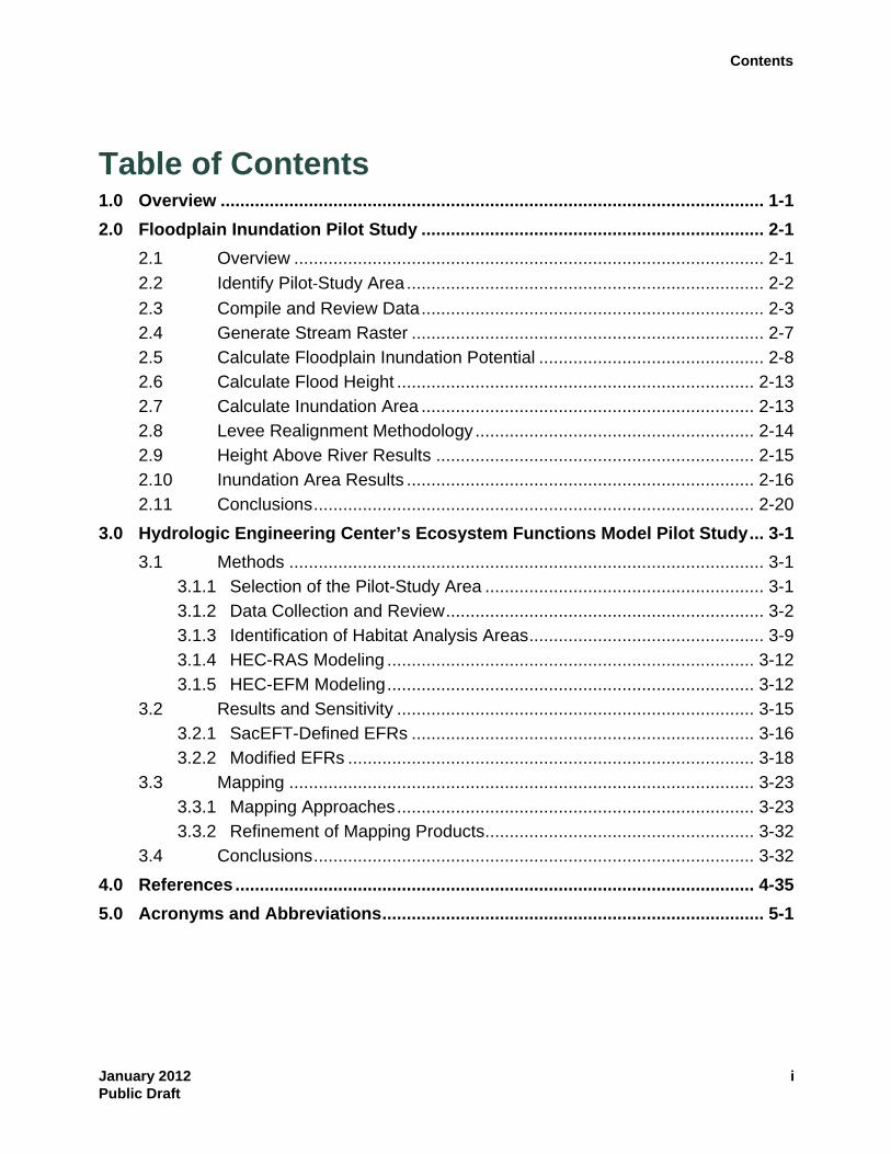
Table of Contents 1.0 Overview ............................................................................................................... 1-1
2.0 Floodplain Inundation Pilot Study ...................................................................... 2-1
2.1 Overview ................................................................................................ 2-1 2.2 Identify Pilot-Study Area ......................................................................... 2-2
2.3 Compile and Review Data ...................................................................... 2-3 2.4 Generate Stream Raster ........................................................................ 2-7 2.5 Calculate Floodplain Inundation Potential .............................................. 2-8 2.6 Calculate Flood Height ......................................................................... 2-13 2.7 Calculate Inundation Area .................................................................... 2-13 2.8 Levee Realignment Methodology ......................................................... 2-14 2.9 Height Above River Results ................................................................. 2-15 2.10 Inundation Area Results ....................................................................... 2-16 2.11 Conclusions .......................................................................................... 2-20
3.0 Hydrologic Engineering Center’s Ecosystem Functions Model Pilot Study ... 3-1
3.1 Methods ................................................................................................. 3-1 3.1.1 Selection of the Pilot-Study Area ......................................................... 3-1 3.1.2 Data Collection and Review ................................................................. 3-2 3.1.3 Identification of Habitat Analysis Areas ................................................ 3-9 3.1.4 HEC-RAS Modeling ........................................................................... 3-12 3.1.5 HEC-EFM Modeling ........................................................................... 3-12
3.2 Results and Sensitivity ......................................................................... 3-15 3.2.1 SacEFT-Defined EFRs ...................................................................... 3-16 3.2.2 Modified EFRs ................................................................................... 3-18
3.3 Mapping ............................................................................................... 3-23 3.3.1 Mapping Approaches ......................................................................... 3-23 3.3.2 Refinement of Mapping Products ....................................................... 3-32
3.4 Conclusions .......................................................................................... 3-32
4.0 References .......................................................................................................... 4-35
5.0 Acronyms and Abbreviations .............................................................................. 5-1
2012 Central Valley Flood Protection Plan Attachment 9F: Floodplain Restoration Opportunity Analysis Appendix A. Floodplain Inundation and Ecosystem Functions Model Pilot Studies
ii January 2012 Public Draft
List of Tables
Table A-1. Areas of Inundation Depths at 50% and 10% Chance Flood Events ..................................................................................................... 2-20
Table A-2. USGS Gages Within the Pilot-Study Area ....................................... 3-7
Table A-3. Habitat Analysis Areas .................................................................. 3-10
Table A-4. Summary of Ecosystem Functional Relationships ........................ 3-13
Table A-5. HEC-EFM Results – RS 26.25–RS 22.50 ..................................... 3-17
Table A-6. HEC-EFM Results—RS 19.00–RS 13.25 ..................................... 3-17
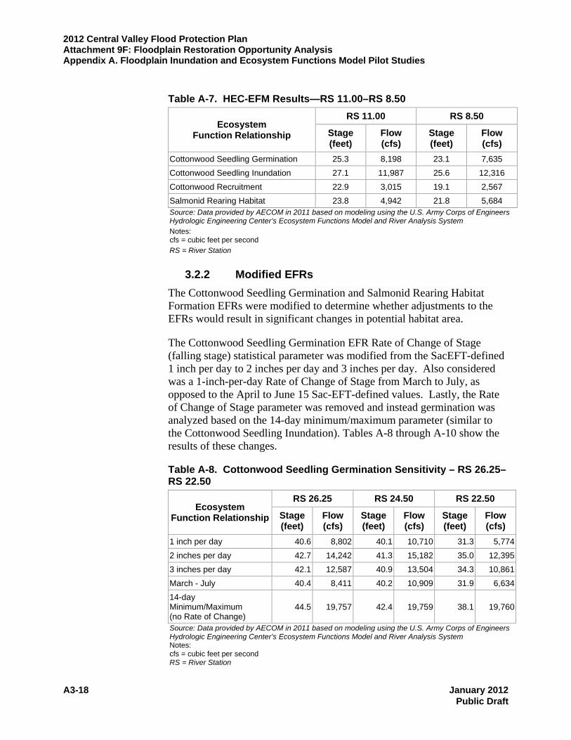
Table A-7. HEC-EFM Results—RS 11.00–RS 8.50 ....................................... 3-18
Table A-8. Cottonwood Seedling Germination Sensitivity – RS 26.25–RS 22.50 ....................................................................................................... 3-18
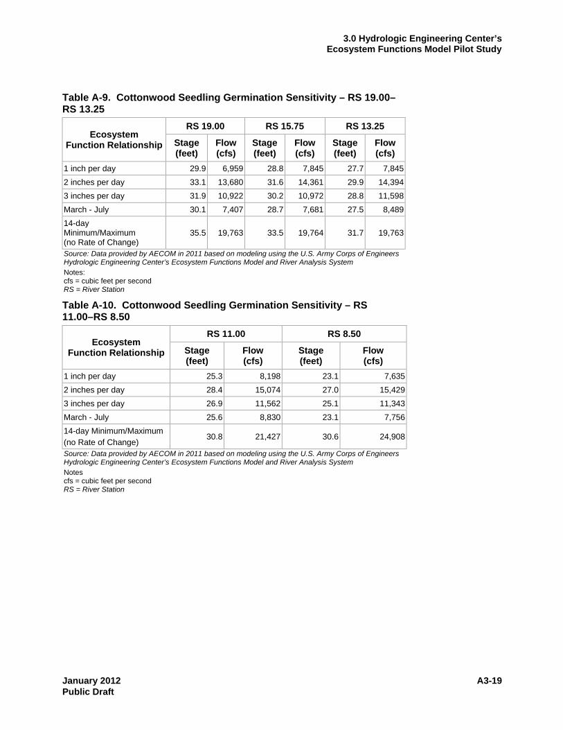
Table A-9. Cottonwood Seedling Germination Sensitivity – RS 19.00–RS 13.25 ....................................................................................................... 3-19
Table A-10. Cottonwood Seedling Germination Sensitivity – RS 11.00–RS 8.50 ......................................................................................................... 3-19
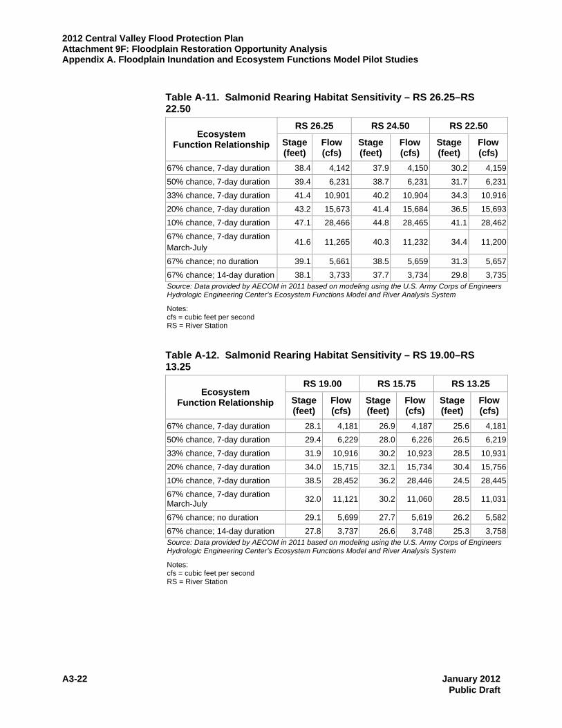
Table A-11. Salmonid Rearing Habitat Sensitivity – RS 26.25–RS 22.50 ...... 3-22
Table A-12. Salmonid Rearing Habitat Sensitivity – RS 19.00–RS 13.25 ...... 3-22
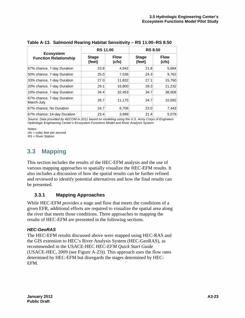
Table A-13. Salmonid Rearing Habitat Sensitivity – RS 11.00–RS 8.50 ........ 3-23
Table A-14. HEC-RAS-Derived Stages for Salmonid-Rearing Habitat – RS 9.75–RS 11.00 .................................................................................. 3-30
Contents
January 2012 iii Public Draft
List of Figures
Figure A-1. Proposed Approach for CVFPP Floodplain Restoration Opportunity Analysis ................................................................................. 2-1
Figure A-2. Lower Feather River Pilot-Study Area ............................................ 2-4
Figure A-3. Central Valley NGVD29 to NAVD88 Vertical Datum Conversion (NAVD88 elevations are higher than NGVD29 elevations)........................ 2-6
Figure A-4. Toolbox Folder Structure ............................................................... 2-8
Figure A-5. Output Stream Raster (5a) and Output Stream Line (5b) .............. 2-9
Figure A-6. HAR Tool Methodology ................................................................ 2-10
Figure A-7. Raster to Point ............................................................................. 2-11
Figure A-8. HAR Closeup (8a) and Pilot Study Reach (8b) ............................ 2-12
Figure A-9. Calculate Inundation Area ............................................................ 2-14
Figure A-10. LiDAR Water-Surface Profile FIP Output ................................... 2-15
Figure A-11. 50 Percent Chance Water-Surface Profile FIP Output ............... 2-17
Figure A-12. 10 Percent Chance Water-Surface Profile FIP Output ............... 2-18
Figure A-13. Cross Section of 50 Percent Chance Flood Profile (RS 19.00) .. 2-19
Figure A-14. Lower Feather River Pilot-Study Area .......................................... 3-3
Figure A-15. Revised HEC-RAS Model ................ Error! Bookmark not defined.
Figure A-16. Synthetic vs. Observed Daily-Averaged Flow – Nicolaus ............ 3-7
Figure A-17. Synthetic vs. Observed Flow Duration Curve – Nicolaus ............. 3-8
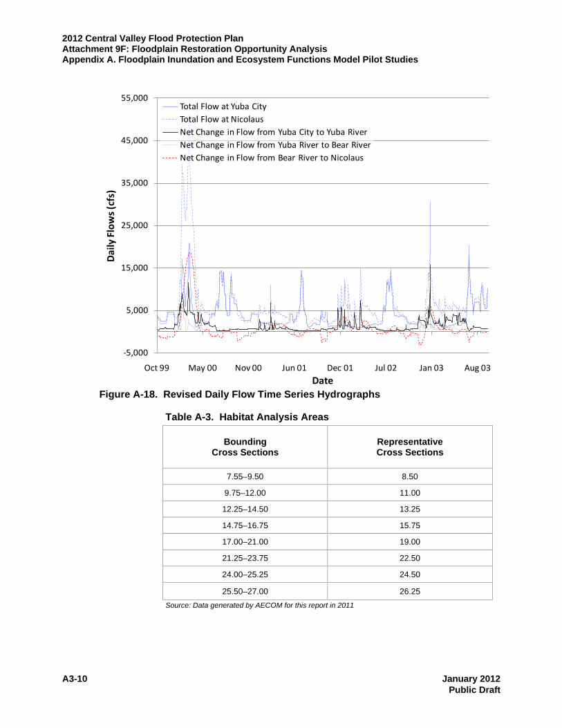
Figure A-18. Revised Daily Flow Time Series Hydrographs ........................... 3-10
Figure A-19. Habitat Analysis Areas ............................................................... 3-11
Figure A-20. Comparison of Rating Curves – RS 11.00 ................................. 3-15
Figure A-21. Comparison of Rating Curves Showing HEC-EFM Results – RS 11.00 ................................................................................................. 3-16
2012 Central Valley Flood Protection Plan Attachment 9F: Floodplain Restoration Opportunity Analysis Appendix A. Floodplain Inundation and Ecosystem Functions Model Pilot Studies
iv January 2012 Public Draft
Figure A-22. Salmonid Rearing Habitat for Various Frequency Events in HAA 11.00 ............................................................................................... 3-24
Figure A-23. Salmonid-Rearing Habitat Areas Mapped Using HEC-GeoRAS in HAA 11.00 ............................................................................ 3-25
Figure A-24. Cottonwood Seedling Germination Habitat Areas Mapped Using FIP and HEC-GeoRAS in HAA 11.00 ............................................ 3-29
Figure A-25. Salmonid-Rearing Habitat Areas Mapped Using FIP and ArcGIS in HAA 11.00 ............................................................................... 3-31

1.0 Overview
January 2012 A1-1 Public Draft
1.0 Overview This appendix provides the methods, results, and conclusions of two pilot studies conducted on the lower Feather River to evaluate the suitability of floodplain inundation potential (FIP) (also known as Height Above River (HAR)) (Dilts et al., 2010) and U.S. Army Corps of Engineers (USACE) Hydrologic Engineering Center’s Ecosystem Functions Model (HEC-EFM) analyses for use in the Floodplain Restoration Opportunity Analysis (FROA). Each pilot study is discussed in a separate section:
• 2.0, Floodplain Inundation Pilot Study
• 3.0, Hydrologic Engineering Center’s Ecosystem Functions Model Pilot Study
The approach of the FROA was developed in part from the results and conclusions of these pilot studies.

2012 Central Valley Flood Protection Plan Attachment 9F: Floodplain Restoration Opportunity Analysis Appendix A. Floodplain Inundation and Ecosystem Functions Model Pilot Studies
A1-2 January 2012 Public Draft
This page left blank intentionally.
2.0 Floodplain Inundation Pilot Study
January 2012 A2-1 Public Draft
2.0 Floodplain Inundation Pilot Study
2.1 Overview
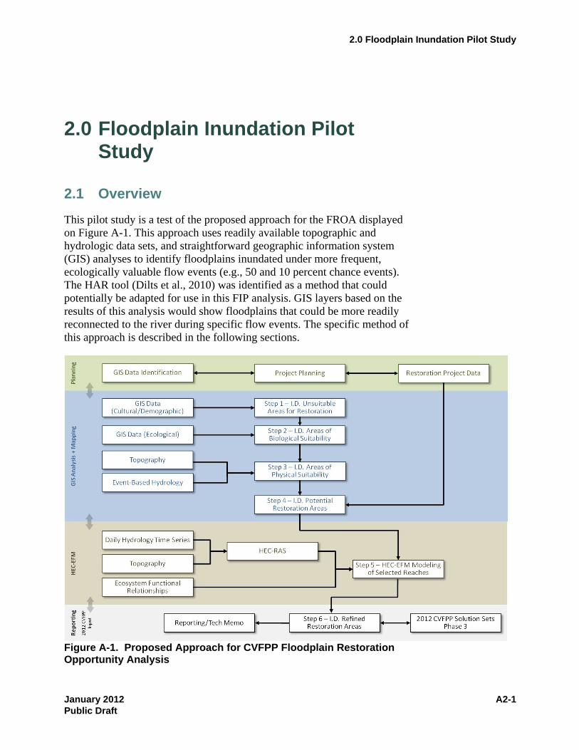
This pilot study is a test of the proposed approach for the FROA displayed on Figure A-1. This approach uses readily available topographic and hydrologic data sets, and straightforward geographic information system (GIS) analyses to identify floodplains inundated under more frequent, ecologically valuable flow events (e.g., 50 and 10 percent chance events). The HAR tool (Dilts et al., 2010) was identified as a method that could potentially be adapted for use in this FIP analysis. GIS layers based on the results of this analysis would show floodplains that could be more readily reconnected to the river during specific flow events. The specific method of this approach is described in the following sections.
Figure A-1. Proposed Approach for CVFPP Floodplain Restoration Opportunity Analysis
2012 Central Valley Flood Protection Plan Attachment 9F: Floodplain Restoration Opportunity Analysis Appendix A. Floodplain Inundation and Ecosystem Functions Model Pilot Studies
A2-2 January 2012 Public Draft
For the purpose of this work, the “FIP method” is the term used to describe a series of GIS tools provided within the Riparian Topography Toolbox, as described by Dilts et al. (2010). These tools are distributed as the ArcGIS Riparian Topography Toolbox by Environmental Systems Research Institute, Inc. (ESRI) (ESRI, 2011).
Through our review and application of the publically available tools in this toolbox, and with the use of unpublished tools provided by Mr. Dilts, we have established a series of steps that constitute the FIP method. These steps are described in the following sections:
• 2.2, Identify Pilot-Study Area
• 2.3, Compile and Review Data
• 2.4, Generate Stream Raster
• 2.5, Calculate Flooplain Inundation Potential
• 2.6, Calculate Flood Height
• 2.7, Calculate Inundation Area
The Riparian Topography Toolbox tools were developed for application to actual river water surface conditions at the time of a Light Detection and Ranging (LiDAR) flight. Since an objective of this pilot study was to investigate the application of these tools to hypothetical flood conditions, other than observed water surface conditions, some deviations were made in the application of the tools; however, the Generate Stream Raster tool was common to all applications.
Section 2.8 describes notes that data were modified to account for two locations in the pilot study area, two locations where levees had been set back after the March 2008 date of the LiDAR flight. Sections 2.9 through 2.11 provide the height above river results, inundation area results, and the conclusions of this pilot study, respectively.
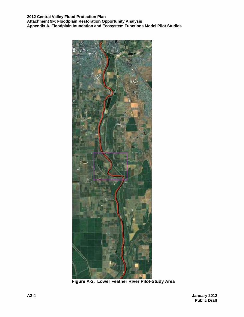
2.2 Identify Pilot-Study Area
An approximately 20-mile reach of the Feather River was selected for the pilot study from the confluence with the Sutter Bypass, upstream to Yuba City at River Station (RS) 27.75 (Figure A-2); the purple rectangle shown on Figure A-2 indicates the specific subreach to which the FIP method was applied.
2.0 Floodplain Inundation Pilot Study
January 2012 A2-3 Public Draft
2.3 Compile and Review Data
The following data were compiled and reviewed in preparation for the application of the HAR tool to the pilot-study area.
1. Terrain Data – Central Valley Floodplain Evaluation and Delineation (CVFED) preprocessed LiDAR and breakline data were obtained and processed into 25-foot digital elevation models (DEM).
2. Water-Surface Profiles – The following water-surface profiles were used in the pilot study:
a. March 2008 LiDAR water-surface profiles – The river water surfaces at the time of the LiDAR flight were used for initial investigations of the relationship of water levels to floodplain inundation.
b. Ten- and 20-foot test profiles – Arbitrary heights of 10 and 20 feet above the LiDAR water surface were used initially to evaluate floodplain inundation areas from higher water levels; these heights were replaced by the Sacramento and San Joaquin River Basins Comprehensive Study (Comprehensive Study) (USACE and The Reclamation Board 2002) 50 and 10 percent chance water-surface profiles for further investigations.
c. Comprehensive Study 50 and 20 percent chance event water-surface profiles – Water-surface profiles for these two return period flood events were obtained by running the Comprehensive Study’s model derived from the USACE Hydrologic Engineering Center’s River Analysis System (HEC-RAS) for the pilot study river reach.
d. Vertical datum conversion – Water surface elevations from the HEC-RAS models are in the older National Geodetic Vertical Datum of 1929 (NGVD29) vertical datum and were converted to the current North American Vertical Datum 1988 (NAVD88) vertical datum to match the vertical datum of the terrain data. Figure A-3 summarizes the spatial variation of the conversion factors in the Central Valley. An average of the conversion factors along the pilot-study stream reach was estimated and this value of +2.335 feet was applied to the HEC-RAS NGVD29 elevations to estimate the NAVD88 elevations.
2012 Central Valley Flood Protection Plan Attachment 9F: Floodplain Restoration Opportunity Analysis Appendix A. Floodplain Inundation and Ecosystem Functions Model Pilot Studies
A2-4 January 2012 Public Draft
Figure A-2. Lower Feather River Pilot-Study Area
2.0 Floodplain Inundation Pilot Study
January 2012 A2-5 Public Draft
The vertical datum conversion was cross-checked by identifying the latitude/longitude of the pilot-study reach and entering this into the National Geodetic Survey (NGS) on-line tool VERTCON (NGS, 2011) to perform the conversion, and the results were similar.
ArcGIS Riparian Topography Toolbox – The Riparian Topography Toolbox for ArcGIS was downloaded from the ESRI Web site (ESRI, 2011). The HAR tool is one of the tools contained within the Riparian Topography Toolbox and includes tools for calculating FIP, inundation area for a given FIP, and flood height.
The FIP method requires the use of a DEM terrain surface. Two sources of DEMs were evaluated for use in the pilot study: (1) U.S. Geological Survey (USGS) 10-meter DEMs (USGS, 2010), and (2) CVFED preliminary DEMs (DWR, 2010b).

2012 Central Valley Flood Protection Plan Attachment 9F: Floodplain Restoration Opportunity Analysis Appendix A. Floodplain Inundation and Ecosystem Functions Model Pilot Studies
A2-6 January 2012 Public Draft
Figure A-3. Central Valley NGVD29 to NAVD88 Vertical Datum Conversion (NAVD88 elevations are higher than NGVD29 elevations)
2.0 Floodplain Inundation Pilot Study
January 2012 A2-7 Public Draft
USGS 10-meter DEMs (USGS, 2010) were obtained and evaluated for their appropriateness of use in the pilot study. Appendix D6-B provides the methods and results of a brief assessment of the data, which led to the decision not to use the USGS data because of the significant inaccuracies found in the delineation of project levees and ground elevations.
New DEMs are being prepared as part of the CVFED program, though the final DEMs have not been completed. Available preliminary CVFED terrain data were obtained for the pilot-study area in October 2010, for use in preparing a DEM for the pilot-study area. The DEM preparation involved incorporating/building breaklines and filling in void areas found in these preliminary CVFED data. The LiDAR data had data voids where water and dense vegetation restricted the triangular irregular network (TIN) from triangulating, essentially leaving large gaps in the TIN. Points were created in those areas to help complete the TIN.
A brief comparison was done to determine the level of effort and resulting data file sizes for the preparation of a DEM with a 5-, 25-, 50-, and 100-foot grid cell resolution (Appendix D6-C). Based on the results of this comparison, DWR decided to develop a 25-foot DEM using preprocessed CVFED data in the pilot-study area. The use of a 25-foot-resolution DEM was determined to provide a reasonable balance between the preparation time, resolution (usability), and file sizes with the intended level of detail for the final products from this planning-level exercise.
2.4 Generate Stream Raster
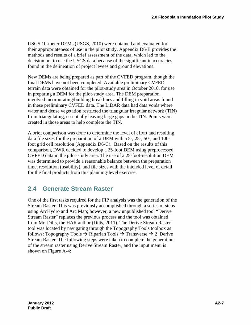
One of the first tasks required for the FIP analysis was the generation of the Stream Raster. This was previously accomplished through a series of steps using ArcHydro and Arc Map; however, a new unpublished tool “Derive Stream Raster” replaces the previous process and the tool was obtained from Mr. Dilts, the HAR author (Dilts, 2011). The Derive Stream Raster tool was located by navigating through the Topography Tools toolbox as follows: Topography Tools Riparian Tools Transverse 2_Derive Stream Raster. The following steps were taken to complete the generation of the stream raster using Derive Stream Raster, and the input menu is shown on Figure A-4:
2012 Central Valley Flood Protection Plan Attachment 9F: Floodplain Restoration Opportunity Analysis Appendix A. Floodplain Inundation and Ecosystem Functions Model Pilot Studies
A2-8 January 2012 Public Draft
Figure A-4. Toolbox Folder Structure
1. Input Elevation Raster – Enter the file location for the 25-foot DEM.
2. Input Start Point and Input End Point – Create two new shapefiles, each consisting of one point named “Start Point” and the other “End Point.” In the Start Point shapefile, a point was placed at the start (upstream limit) of the pilot-study stream reach of interest. In End Point shapefile, a point was placed at the end (downstream limit) of the pilot-study stream reach of interest. The DEM was used as a visual aid to locate these points along the centerline of the stream channel.
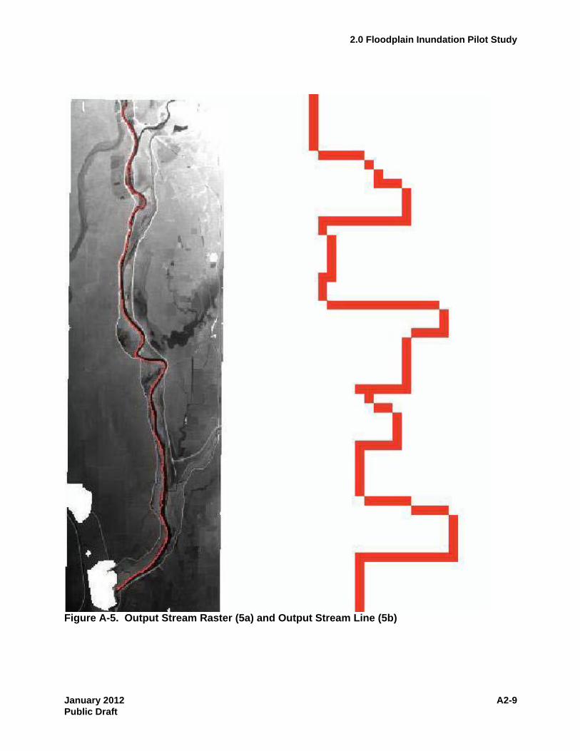
3. Output Stream Raster – Assign name and location to place output stream raster grid cells (Figure A-5a).
4. Output Stream Line – Assign shapefile location and filename for stream raster grids converted to polyline (Figure A-5b).
2.5 Calculate Floodplain Inundation Potential
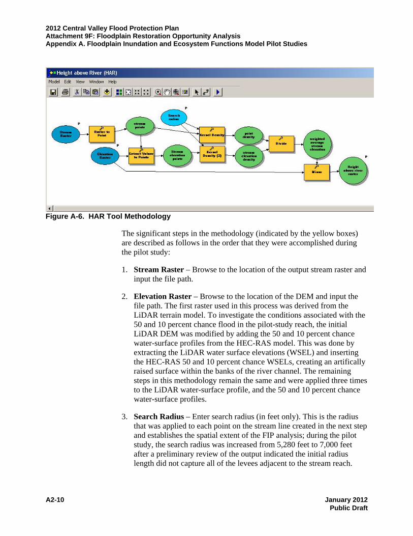
The HAR tool was located by navigating through the Topography Tools toolbox as follows: Topography Tools Riparian Tools Transverse 2_HAR right-click Edit. The HAR tool methodology is shown in a flow chart on Figure A-6, where blue ovals indicate data entry steps, the yellow boxes are tool processes, and the green ovals are outputs from processes.
2.0 Floodplain Inundation Pilot Study
January 2012 A2-9 Public Draft
Figure A-5. Output Stream Raster (5a) and Output Stream Line (5b)
2012 Central Valley Flood Protection Plan Attachment 9F: Floodplain Restoration Opportunity Analysis Appendix A. Floodplain Inundation and Ecosystem Functions Model Pilot Studies
A2-10 January 2012 Public Draft
Figure A-6. HAR Tool Methodology
The significant steps in the methodology (indicated by the yellow boxes) are described as follows in the order that they were accomplished during the pilot study:
1. Stream Raster – Browse to the location of the output stream raster and input the file path.
2. Elevation Raster – Browse to the location of the DEM and input the file path. The first raster used in this process was derived from the LiDAR terrain model. To investigate the conditions associated with the 50 and 10 percent chance flood in the pilot-study reach, the initial LiDAR DEM was modified by adding the 50 and 10 percent chance water-surface profiles from the HEC-RAS model. This was done by extracting the LiDAR water surface elevations (WSEL) and inserting the HEC-RAS 50 and 10 percent chance WSELs, creating an artifically raised surface within the banks of the river channel. The remaining steps in this methodology remain the same and were applied three times to the LiDAR water-surface profile, and the 50 and 10 percent chance water-surface profiles.
3. Search Radius – Enter search radius (in feet only). This is the radius that was applied to each point on the stream line created in the next step and establishes the spatial extent of the FIP analysis; during the pilot study, the search radius was increased from 5,280 feet to 7,000 feet after a preliminary review of the output indicated the initial radius length did not capture all of the levees adjacent to the stream reach.
2.0 Floodplain Inundation Pilot Study
January 2012 A2-11 Public Draft
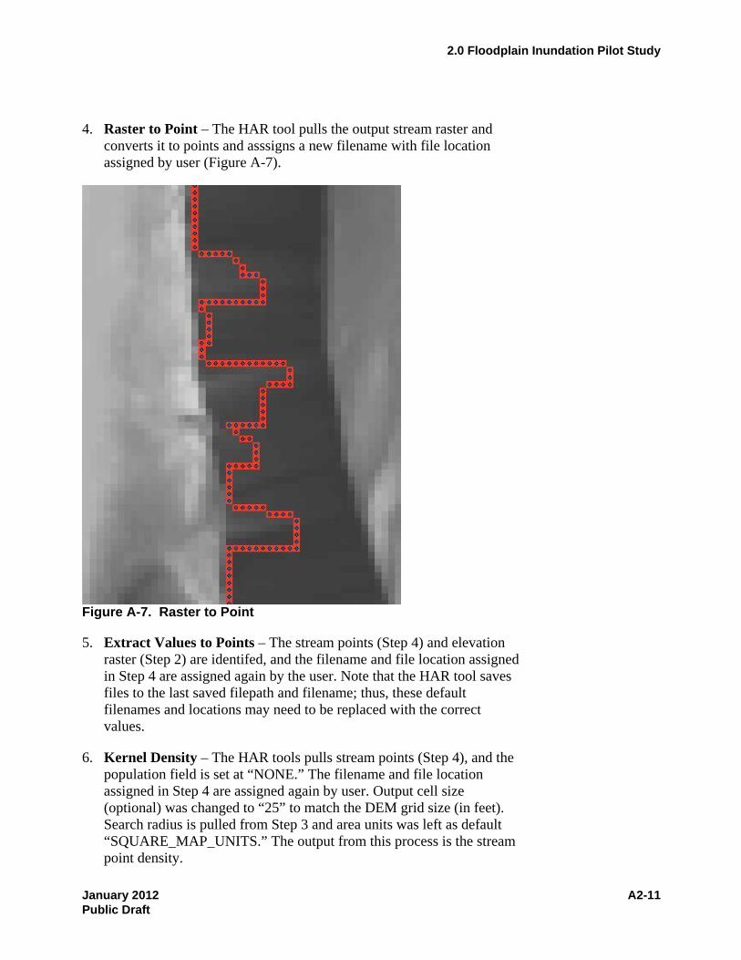
4. Raster to Point – The HAR tool pulls the output stream raster and converts it to points and asssigns a new filename with file location assigned by user (Figure A-7).
Figure A-7. Raster to Point
5. Extract Values to Points – The stream points (Step 4) and elevation raster (Step 2) are identifed, and the filename and file location assigned in Step 4 are assigned again by the user. Note that the HAR tool saves files to the last saved filepath and filename; thus, these default filenames and locations may need to be replaced with the correct values.
6. Kernel Density – The HAR tools pulls stream points (Step 4), and the population field is set at “NONE.” The filename and file location assigned in Step 4 are assigned again by user. Output cell size (optional) was changed to “25” to match the DEM grid size (in feet). Search radius is pulled from Step 3 and area units was left as default “SQUARE_MAP_UNITS.” The output from this process is the stream point density.
2012 Central Valley Flood Protection Plan Attachment 9F: Floodplain Restoration Opportunity Analysis Appendix A. Floodplain Inundation and Ecosystem Functions Model Pilot Studies
A2-12 January 2012 Public Draft
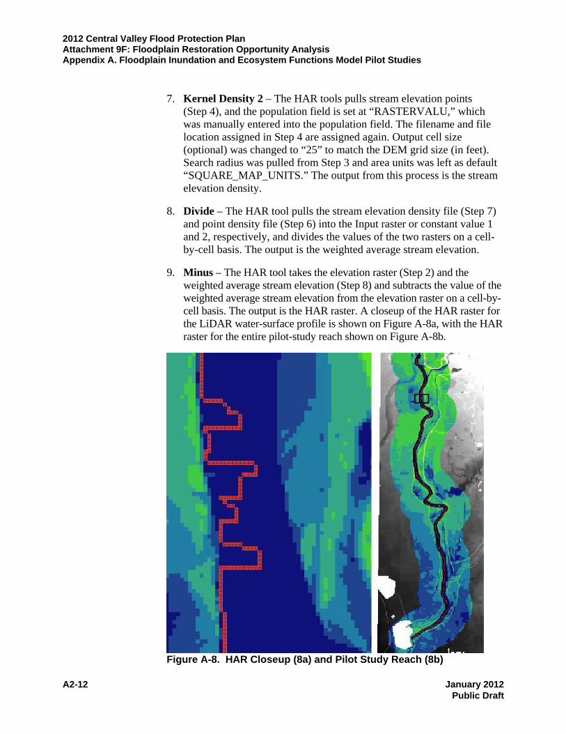
7. Kernel Density 2 – The HAR tools pulls stream elevation points (Step 4), and the population field is set at “RASTERVALU,” which was manually entered into the population field. The filename and file location assigned in Step 4 are assigned again. Output cell size (optional) was changed to “25” to match the DEM grid size (in feet). Search radius was pulled from Step 3 and area units was left as default “SQUARE_MAP_UNITS.” The output from this process is the stream elevation density.
8. Divide – The HAR tool pulls the stream elevation density file (Step 7) and point density file (Step 6) into the Input raster or constant value 1 and 2, respectively, and divides the values of the two rasters on a cell-by-cell basis. The output is the weighted average stream elevation.
9. Minus – The HAR tool takes the elevation raster (Step 2) and the weighted average stream elevation (Step 8) and subtracts the value of the weighted average stream elevation from the elevation raster on a cell-by-cell basis. The output is the HAR raster. A closeup of the HAR raster for the LiDAR water-surface profile is shown on Figure A-8a, with the HAR raster for the entire pilot-study reach shown on Figure A-8b.
Figure A-8. HAR Closeup (8a) and Pilot Study Reach (8b)
2.0 Floodplain Inundation Pilot Study
January 2012 A2-13 Public Draft
2.6 Calculate Flood Height
A Calculate Flood Height tool is provided in the Riparian Topography Tools toolbox; however, in lieu of this approach, flood height was estimated by changing the symbology of the HAR raster. This method proved to be quicker, provided equivalent results, and involved the following steps:
1. The HAR raster was brought into ArcMap. Pyramids were built when prompted to improve image quality.
2. The HAR raster Properties were selected by right-clicking the HAR raster and clicking Properties.
3. Layer Properties – The Symbology tab was selected and the Show entered “Classified” was choosen and Compute Histogram was activated by clicking Yes when prompted.
4. Classification – The Natural Breaks (Jenks) – The Classify button was clicked to open the Classification menu box. User selects number of Breaks.
5. Break Values – These values were set so the lowest value in the HAR raster was in the same Break Value range as the height of the flooding. No other values were changed because the flood height was the only value necessary. The OK button was selected when values were set.
6. Layer Properties – Color Ramp – Symbol, Range, Label – The symbol for the range containing the lowest HAR raster value and the flood height value was changed to a color different from the rest of the ranges.
2.7 Calculate Inundation Area
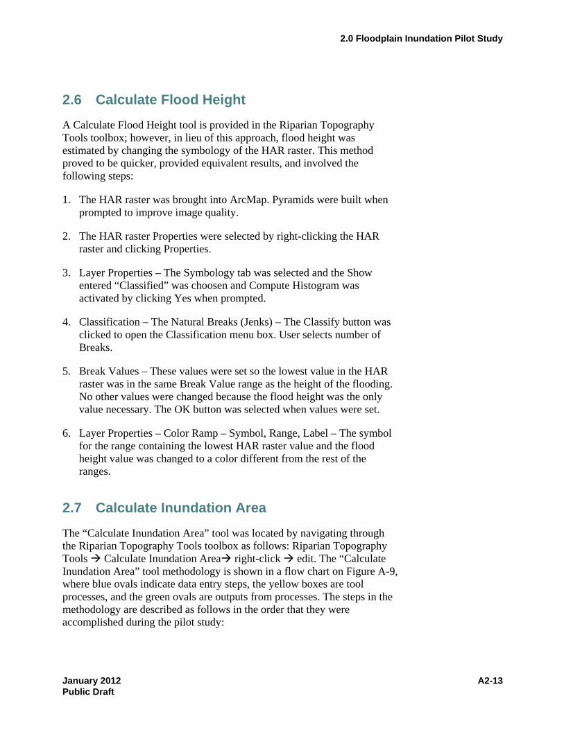
The “Calculate Inundation Area” tool was located by navigating through the Riparian Topography Tools toolbox as follows: Riparian Topography Tools Calculate Inundation Area right-click edit. The “Calculate Inundation Area” tool methodology is shown in a flow chart on Figure A-9, where blue ovals indicate data entry steps, the yellow boxes are tool processes, and the green ovals are outputs from processes. The steps in the methodology are described as follows in the order that they were accomplished during the pilot study:
2012 Central Valley Flood Protection Plan Attachment 9F: Floodplain Restoration Opportunity Analysis Appendix A. Floodplain Inundation and Ecosystem Functions Model Pilot Studies
A2-14 January 2012 Public Draft
Figure A-9. Calculate Inundation Area
1. Height above River Raster – Browse to location of HAR raster and input file path.
2. Input streams – Browse to location of stream raster and input file path.
3. Expression (optional) – The value entered here is the height above the FIP water-surface profile, and it sets threshold elevation and code values either above or below this surface, with the cells below the FIP value directly connected to the river. Through trial and error we determined that the minimum value to enter here is 1.0 foot owing to the elevation variability imposed on the true water surface by the FIP method.
4. Output flood zone – Assign raster location and filename for inundation area.
2.8 Levee Realignment Methodology
Within the Feather River pilot-study reach, the project team noted that there were two locations where levees had been set back after the March 2008 date of the LiDAR flight. This resulted in a need to adjust the DEM terrain surface to show actual current topographic conditions. While the FIP output in this technical memorandum still shows the March 2008 levee
2.0 Floodplain Inundation Pilot Study
January 2012 A2-15 Public Draft
positions, a separate effort was made to determine a reasonable methodology to adjust levee locations for subsequent FIP analyses. This methodology is described in Appendix D6-D.
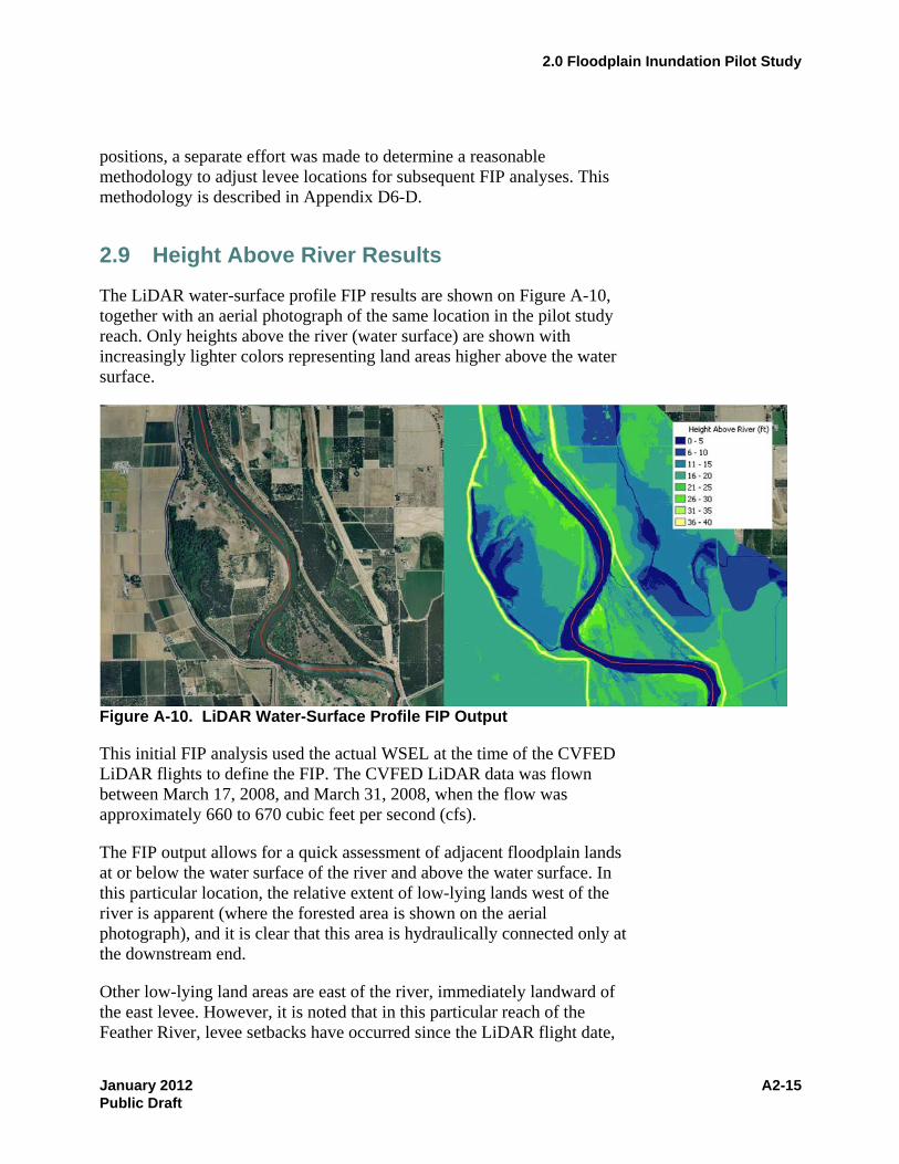
2.9 Height Above River Results
The LiDAR water-surface profile FIP results are shown on Figure A-10, together with an aerial photograph of the same location in the pilot study reach. Only heights above the river (water surface) are shown with increasingly lighter colors representing land areas higher above the water surface.
Figure A-10. LiDAR Water-Surface Profile FIP Output
This initial FIP analysis used the actual WSEL at the time of the CVFED LiDAR flights to define the FIP. The CVFED LiDAR data was flown between March 17, 2008, and March 31, 2008, when the flow was approximately 660 to 670 cubic feet per second (cfs).
The FIP output allows for a quick assessment of adjacent floodplain lands at or below the water surface of the river and above the water surface. In this particular location, the relative extent of low-lying lands west of the river is apparent (where the forested area is shown on the aerial photograph), and it is clear that this area is hydraulically connected only at the downstream end.
Other low-lying land areas are east of the river, immediately landward of the east levee. However, it is noted that in this particular reach of the Feather River, levee setbacks have occurred since the LiDAR flight date,
2012 Central Valley Flood Protection Plan Attachment 9F: Floodplain Restoration Opportunity Analysis Appendix A. Floodplain Inundation and Ecosystem Functions Model Pilot Studies
A2-16 January 2012 Public Draft
and a portion of the levee locations shown on Figure A-10 are outdated. A technique was developed to realign levees on the DEM; this method was discussed in Section 2.2.8 and will be applied to levee sections where recent restoration projects have resulted in a change in levee alignments since the LiDAR flights in March 2008.
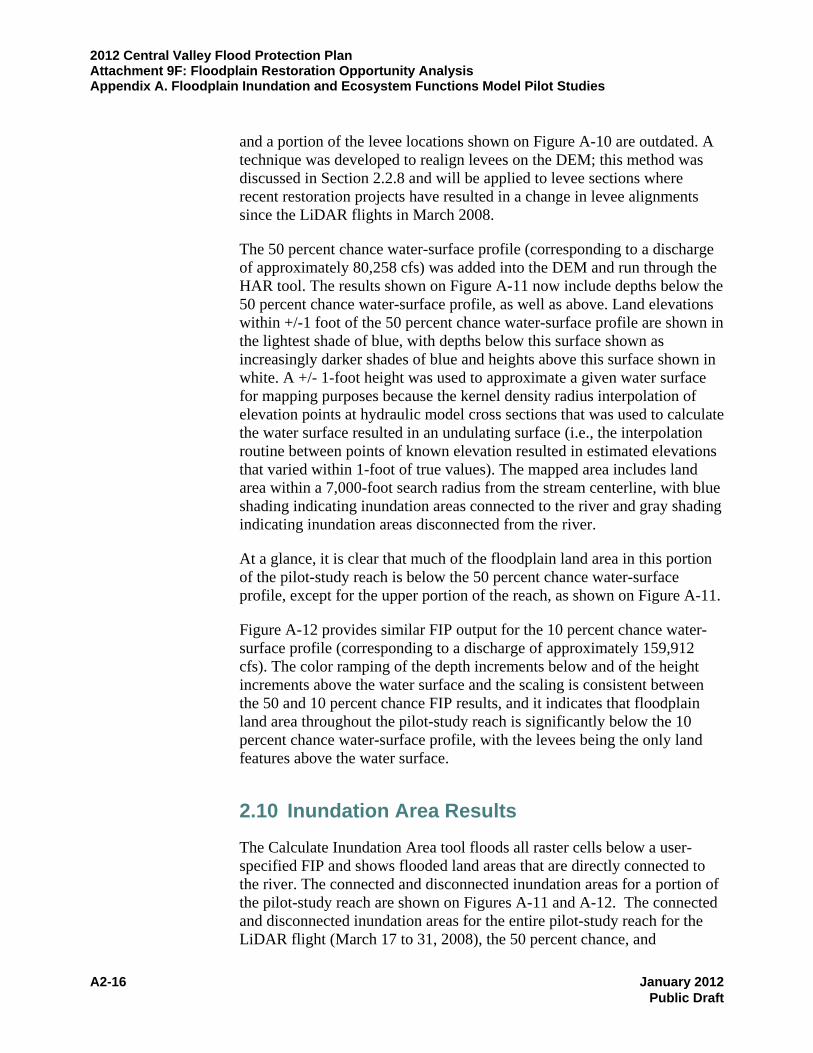
The 50 percent chance water-surface profile (corresponding to a discharge of approximately 80,258 cfs) was added into the DEM and run through the HAR tool. The results shown on Figure A-11 now include depths below the 50 percent chance water-surface profile, as well as above. Land elevations within +/-1 foot of the 50 percent chance water-surface profile are shown in the lightest shade of blue, with depths below this surface shown as increasingly darker shades of blue and heights above this surface shown in white. A +/- 1-foot height was used to approximate a given water surface for mapping purposes because the kernel density radius interpolation of elevation points at hydraulic model cross sections that was used to calculate the water surface resulted in an undulating surface (i.e., the interpolation routine between points of known elevation resulted in estimated elevations that varied within 1-foot of true values). The mapped area includes land area within a 7,000-foot search radius from the stream centerline, with blue shading indicating inundation areas connected to the river and gray shading indicating inundation areas disconnected from the river.
At a glance, it is clear that much of the floodplain land area in this portion of the pilot-study reach is below the 50 percent chance water-surface profile, except for the upper portion of the reach, as shown on Figure A-11.
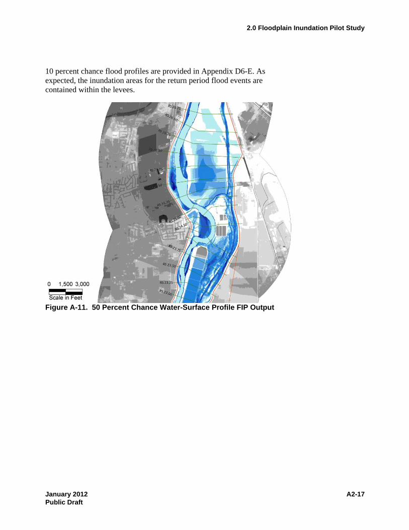
Figure A-12 provides similar FIP output for the 10 percent chance water-surface profile (corresponding to a discharge of approximately 159,912 cfs). The color ramping of the depth increments below and of the height increments above the water surface and the scaling is consistent between the 50 and 10 percent chance FIP results, and it indicates that floodplain land area throughout the pilot-study reach is significantly below the 10 percent chance water-surface profile, with the levees being the only land features above the water surface.
2.10 Inundation Area Results
The Calculate Inundation Area tool floods all raster cells below a user-specified FIP and shows flooded land areas that are directly connected to the river. The connected and disconnected inundation areas for a portion of the pilot-study reach are shown on Figures A-11 and A-12. The connected and disconnected inundation areas for the entire pilot-study reach for the LiDAR flight (March 17 to 31, 2008), the 50 percent chance, and
2.0 Floodplain Inundation Pilot Study
January 2012 A2-17 Public Draft
10 percent chance flood profiles are provided in Appendix D6-E. As expected, the inundation areas for the return period flood events are contained within the levees.
Figure A-11. 50 Percent Chance Water-Surface Profile FIP Output
2012 Central Valley Flood Protection Plan Attachment 9F: Floodplain Restoration Opportunity Analysis Appendix A. Floodplain Inundation and Ecosystem Functions Model Pilot Studies
A2-18 January 2012 Public Draft
Figure A-12. 10 Percent Chance Water-Surface Profile FIP Output
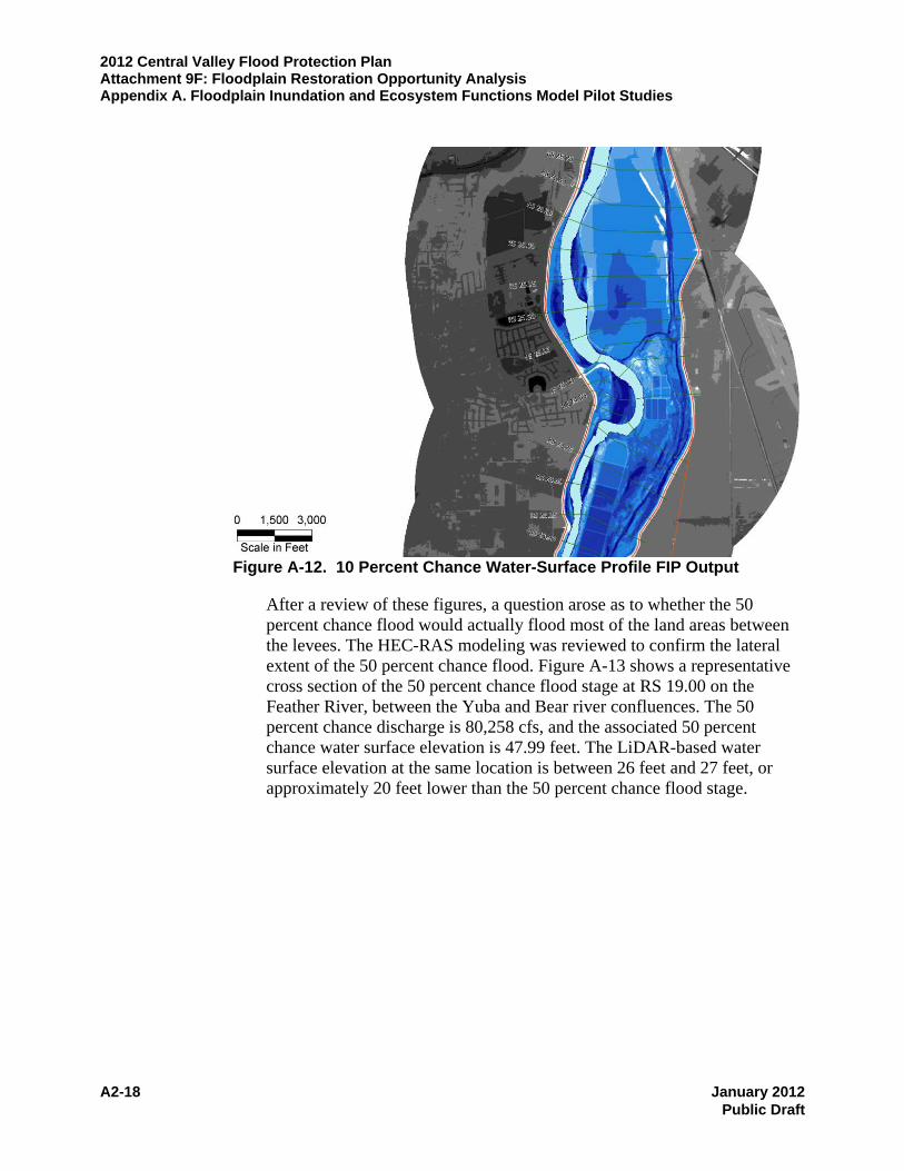
After a review of these figures, a question arose as to whether the 50 percent chance flood would actually flood most of the land areas between the levees. The HEC-RAS modeling was reviewed to confirm the lateral extent of the 50 percent chance flood. Figure A-13 shows a representative cross section of the 50 percent chance flood stage at RS 19.00 on the Feather River, between the Yuba and Bear river confluences. The 50 percent chance discharge is 80,258 cfs, and the associated 50 percent chance water surface elevation is 47.99 feet. The LiDAR-based water surface elevation at the same location is between 26 feet and 27 feet, or approximately 20 feet lower than the 50 percent chance flood stage.
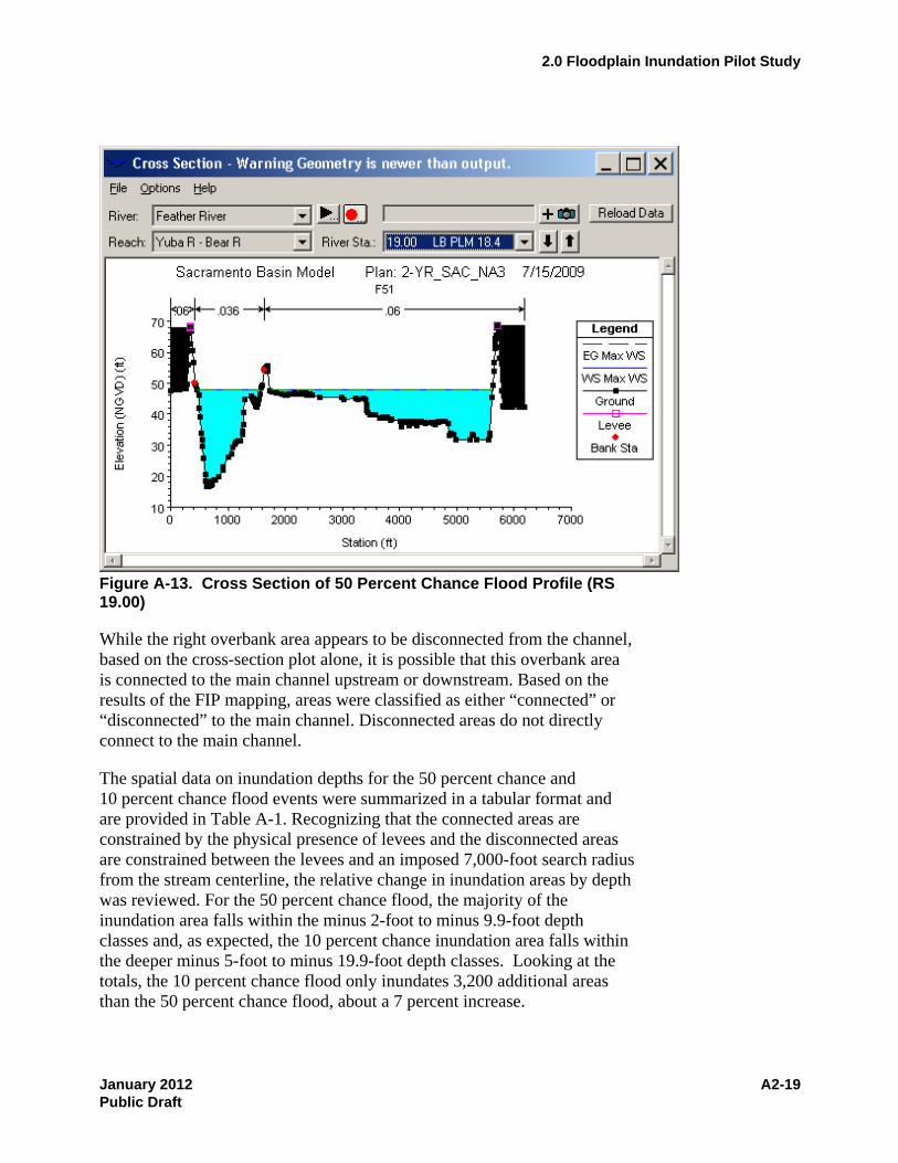
2.0 Floodplain Inundation Pilot Study
January 2012 A2-19 Public Draft
Figure A-13. Cross Section of 50 Percent Chance Flood Profile (RS 19.00)
While the right overbank area appears to be disconnected from the channel, based on the cross-section plot alone, it is possible that this overbank area is connected to the main channel upstream or downstream. Based on the results of the FIP mapping, areas were classified as either “connected” or “disconnected” to the main channel. Disconnected areas do not directly connect to the main channel.
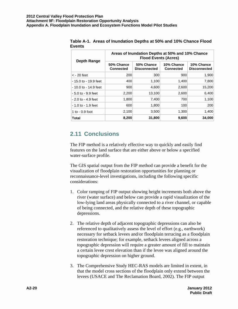
The spatial data on inundation depths for the 50 percent chance and 10 percent chance flood events were summarized in a tabular format and are provided in Table A-1. Recognizing that the connected areas are constrained by the physical presence of levees and the disconnected areas are constrained between the levees and an imposed 7,000-foot search radius from the stream centerline, the relative change in inundation areas by depth was reviewed. For the 50 percent chance flood, the majority of the inundation area falls within the minus 2-foot to minus 9.9-foot depth classes and, as expected, the 10 percent chance inundation area falls within the deeper minus 5-foot to minus 19.9-foot depth classes. Looking at the totals, the 10 percent chance flood only inundates 3,200 additional areas than the 50 percent chance flood, about a 7 percent increase.
2012 Central Valley Flood Protection Plan Attachment 9F: Floodplain Restoration Opportunity Analysis Appendix A. Floodplain Inundation and Ecosystem Functions Model Pilot Studies
A2-20 January 2012 Public Draft
Table A-1. Areas of Inundation Depths at 50% and 10% Chance Flood Events
Depth Range
Areas of Inundation Depths at 50% and 10% Chance Flood Events (Acres)
50% Chance Connected
50% Chance Disconnected
10% Chance Connected
10% Chance Disconnected
< - 20 feet 200 300 900 1,900
- 15.0 to - 19.9 feet 400 1,100 1,400 7,800
- 10.0 to - 14.9 feet 900 4,600 2,600 15,200
- 5.0 to - 9.9 feet 2,200 13,100 2,600 6,400
- 2.0 to - 4.9 feet 1,800 7,400 700 1,100
- 1.0 to - 1.9 feet 600 1,800 100 200
1 to - 0.9 foot 2,100 3,500 1,300 1,400
Total 8,200 31,800 9,600 34,000
2.11 Conclusions
The FIP method is a relatively effective way to quickly and easily find features on the land surface that are either above or below a specified water-surface profile.
The GIS spatial output from the FIP method can provide a benefit for the visualization of floodplain restoration opportunities for planning or reconnaissance-level investigations, including the following specific considerations:
1. Color ramping of FIP output showing height increments both above the river (water surface) and below can provide a rapid visualization of the low-lying land areas physically connected to a river channel, or capable of being connected, and the relative depth of these topographic depressions.
2. The relative depth of adjacent topographic depressions can also be referenced to qualitatively assess the level of effort (e.g., earthwork) necessary for setback levees and/or floodplain terracing as a floodplain restoration technique; for example, setback levees aligned across a topographic depression will require a greater amount of fill to maintain a certain levee crest elevation than if the levee was aligned around the topographic depression on higher ground.
3. The Comprehensive Study HEC-RAS models are limited in extent, in that the model cross sections of the floodplain only extend between the levees (USACE and The Reclamation Board, 2002). The FIP output
2.0 Floodplain Inundation Pilot Study
January 2012 A2-21 Public Draft
provides estimates of flood profile elevations and flood depths beyond the levees, and this information can be used to guide qualitative investigations into potential levee setback locations. Although the FIP method is not a substitute for detailed hydraulic modeling, it does provide an ability to relatively quickly understand flood characteristics across the floodplain landscape.
Mr. Dilts has recently begun to update his tools and has provided his unpublished versions for use on this pilot study. Because of this, the generation of the Stream Raster, which is a very important component to the FIP, is now automated and can be applied more quickly to future FIP investigations.

2012 Central Valley Flood Protection Plan Attachment 9F: Floodplain Restoration Opportunity Analysis Appendix A. Floodplain Inundation and Ecosystem Functions Model Pilot Studies
A2-22 January 2012 Public Draft
This page left blank intentionally.
3.0 Hydrologic Engineering Center’s Ecosystem Functions Model Pilot Study
January 2012 A3-1 Public Draft
3.0 Hydrologic Engineering Center’s Ecosystem Functions Model Pilot Study
This section summarizes the HEC-EFM pilot study in four sections:
• 3.1, Methods
• 3.2, Results and Sensitivity
• 3.3, Mapping
• 3.4, Conclusions
3.1 Methods
This section describes the methods and approaches used to perform the HEC-RAS/HEC-EFM (RAS/EFM) analysis on the lower Feather River near Yuba City, California. As discussed, the goal of this study was to document the standard methods and approaches required for a RAS/EFM analysis and to identify potential issues, if any, and/or alternative approaches. The following tasks were conducted as part of the RAS/EFM analysis:
• Selection of the pilot-study area
• Data collection and review
• Identification of Habitat Analysis Areas (HAA)
• HEC-RAS modeling
• HEC-EFM analysis
The remainder of this section describes these tasks in more detail.
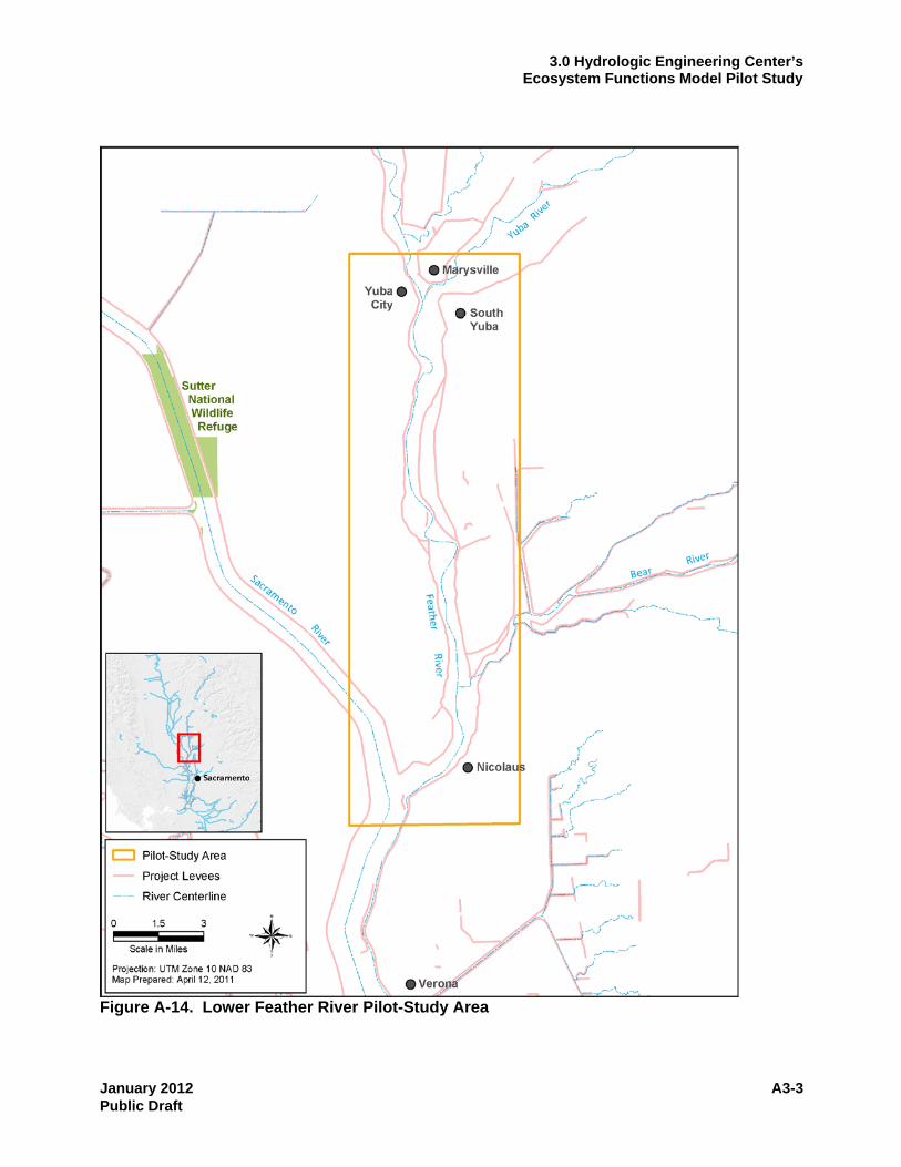
3.1.1 Selection of the Pilot-Study Area The pilot study was conducted on a 21-mile reach of the lower Feather River, from the confluence with the Sutter Bypass, upstream to Yuba City at RS 27.75 (see Figure A-14). The area was chosen for the availability of data and the project team’s familiarity with the area. Within the study area, the lower Feather River maintains levees along both banks and receives
2012 Central Valley Flood Protection Plan Attachment 9F: Floodplain Restoration Opportunity Analysis Appendix A. Floodplain Inundation and Ecosystem Functions Model Pilot Studies
A3-2 January 2012 Public Draft
flow from the Yuba and Bear rivers. It also maintains inflows and outflows resulting from agricultural and groundwater sources.
3.1.2 Data Collection and Review A steady-state, geo-referenced HEC-RAS model of the Feather River, from the confluence with the Sutter Bypass to the Thermalito Afterbay, and synthetic daily flow hydrographs from October 1, 1921, to September 30, 2003, were provided to AECOM by MWH Americas, Inc. (MWH).
The HEC-RAS model was developed by MWH based on the Feather River Sacramento-San Joaquin Comprehensive Study UNET hydraulic model (USACE and The Reclamation Board 2002). MWH converted the original Comprehensive Study UNET model to HEC-RAS, geo-referenced the model, and calibrated the model to low-flow conditions. The model files were provided via FTP on November 30, 2010.
The Feather River synthetic daily flow hydrographs were developed by MWH from monthly flow hydrographs computed by the CalSim model. Hydrographs were provided by MWH via e-mail on December 8, 2010. Development methodology for the synthetic daily flow hydrographs was
3.0 Hydrologic Engineering Center’s Ecosystem Functions Model Pilot Study
January 2012 A3-3 Public Draft
Figure A-14. Lower Feather River Pilot-Study Area
2012 Central Valley Flood Protection Plan Attachment 9F: Floodplain Restoration Opportunity Analysis Appendix A. Floodplain Inundation and Ecosystem Functions Model Pilot Studies
A3-4 January 2012 Public Draft
outlined in a draft document prepared by MWH, titled Feather River Daily Flows for HEC-EFM (2011). This document is currently being finalized by MWH and will be submitted to California Department of Water Resources (DWR) separately from this report.
The following actions were performed during the review and application of the HEC-RAS model and synthetic daily flow hydrographs.
1. The model was reviewed briefly to confirm its appropriateness for this study and to review the geo-referencing, reach lengths, and Manning’s n values. Detailed features or assumptions, such as the value of coefficients, the stations, and elevations of levees and ineffective flows areas, and other detailed aspects of the model were not reviewed.
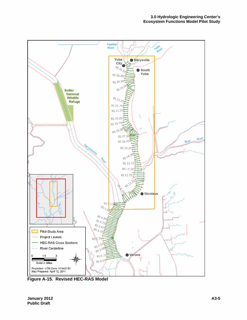
2. Areas of the model upstream from the Feather River and Yuba River confluence were removed and the upstream boundary was set to RS 27.75. This was done to remove unnecessary complexities upstream from the study area. Figure A-15 shows an overview of the revised HEC-RAS model.
3. An unsteady-state version of the model was developed, requiring the following actions:
a. Modification of the model geometry
An inline weir was added at RS 24.00 to improve model stability at the Shanghai Bend Falls, where a sudden change in the channel invert can produce super-critical and unstable conditions. The model was adjusted from the original NGVD29 datum to match the terrain datum, NAVD88, by adding 2.335 feet (see AECOM’s Technical Memorandum (TM) – Height Above River Investigations (AECOM, 2011a)). The model geometry was not updated using the LiDAR-derived DEMs as described in the Scope of Sub-Consultancy Services Subtask 3.3.1.d, “recut floodplain cross-section data, combine with channel geometry.” This task was not performed because official DWR review of LiDAR-derived DEMs was not complete.
3.0 Hydrologic Engineering Center’s Ecosystem Functions Model Pilot Study
January 2012 A3-5 Public Draft
Figure A-15. Revised HEC-RAS Model
2012 Central Valley Flood Protection Plan Attachment 9F: Floodplain Restoration Opportunity Analysis Appendix A. Floodplain Inundation and Ecosystem Functions Model Pilot Studies
A3-6 January 2012 Public Draft
b. Development of unsteady-state boundary conditions
Unsteady-state boundary conditions were developed to simulate the synthetic period. The downstream boundary condition at RS 0.13 was set to normal depth with a friction slope of 0.0002 (0.02 percent). The upstream boundary condition at RS 27.75 was set to read the daily synthetic flow hydrograph provided by MWH at Yuba City. Inflows and outflows between Yuba City and the Sutter Bypass were applied based on the synthetic daily flow hydrographs provided by MWH.
c. Review of synthetic hydrographs
The hydrographs provided by MWH included synthetic daily-average flows from October 1, 1921, to September 30, 2003, at locations along the Feather River. The flows were developed from the CalSim State Water Project (SWP)/Central Valley Project (CVP) monthly simulation model.
The flow in the Feather River is controlled by water operations at the upstream Oroville Reservoir. Because of changes in Oroville operations to meet increasing demands both for water supply and environmental purposes, historical flows may not provide the best representation of future flows in the Feather River.
The CalSim model is specifically designed to evaluate the operations of Oroville Reservoir, and the flows in the Feather River, under potential conditions assuming that the historical precipitation from October 1921 through September 2003 reoccurs. The resulting flows may provide a better representation of expected future flows than historical flows.
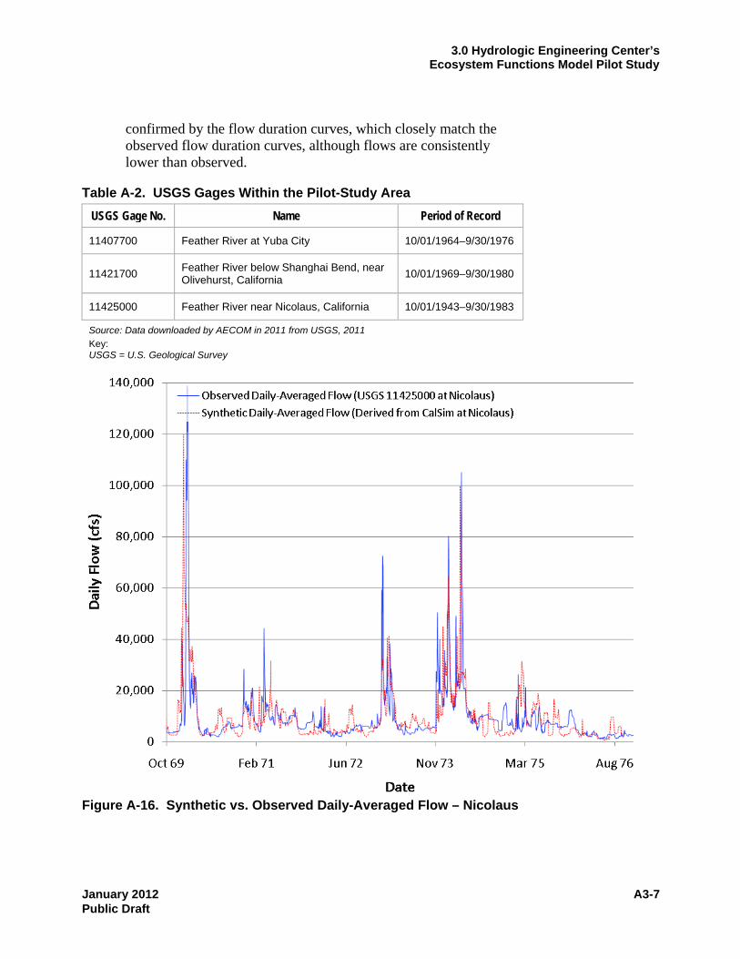
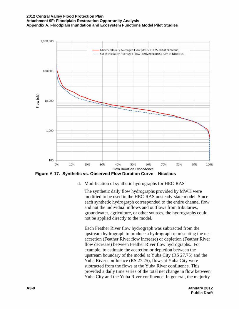
The synthetic daily average flows provided by MWH to observed daily average flows at USGS flow gages (see Table A-2) were compared to determine whether the synthetic flows provided reasonable values. Figures A-16 and A-17 compare daily averaged flows and resulting flow duration curves for the period of October 1, 1969, through September 30, 1976, (Water Year (WY) 1970 through WY 1976) at Nicolaus (see Figures E-1 through E-4 in Appendix D6-E for the Yuba City and Shanghai Bend locations). The selected period of record represents a time frame when the USGS gages were all in operation.
The comparison illustrates that while the synthetic daily averaged flows often do not reproduce individual daily averaged flows, they do reproduce the various high- and low-flow events. This is
3.0 Hydrologic Engineering Center’s Ecosystem Functions Model Pilot Study
January 2012 A3-7 Public Draft
confirmed by the flow duration curves, which closely match the observed flow duration curves, although flows are consistently lower than observed.
Table A-2. USGS Gages Within the Pilot-Study Area USGS Gage No. Name Period of Record
11407700 Feather River at Yuba City 10/01/1964–9/30/1976
11421700 Feather River below Shanghai Bend, near Olivehurst, California 10/01/1969–9/30/1980
11425000 Feather River near Nicolaus, California 10/01/1943–9/30/1983
Source: Data downloaded by AECOM in 2011 from USGS, 2011 Key: USGS = U.S. Geological Survey
Figure A-16. Synthetic vs. Observed Daily-Averaged Flow – Nicolaus
2012 Central Valley Flood Protection Plan Attachment 9F: Floodplain Restoration Opportunity Analysis Appendix A. Floodplain Inundation and Ecosystem Functions Model Pilot Studies
A3-8 January 2012 Public Draft
Figure A-17. Synthetic vs. Observed Flow Duration Curve – Nicolaus
d. Modification of synthetic hydrographs for HEC-RAS
The synthetic daily flow hydrographs provided by MWH were modified to be used in the HEC-RAS unsteady-state model. Since each synthetic hydrograph corresponded to the entire channel flow and not the individual inflows and outflows from tributaries, groundwater, agriculture, or other sources, the hydrographs could not be applied directly to the model.
Each Feather River flow hydrograph was subtracted from the upstream hydrograph to produce a hydrograph representing the net accretion (Feather River flow increase) or depletion (Feather River flow decrease) between Feather River flow hydrographs. For example, to estimate the accretion or depletion between the upstream boundary of the model at Yuba City (RS 27.75) and the Yuba River confluence (RS 27.25), flows at Yuba City were subtracted from the flows at the Yuba River confluence. This provided a daily time series of the total net change in flow between Yuba City and the Yuba River confluence. In general, the majority
3.0 Hydrologic Engineering Center’s Ecosystem Functions Model Pilot Study
January 2012 A3-9 Public Draft
of this change can be attributed to the Yuba River, so the daily time series was applied as the Yuba River inflow hydrograph. This process was repeated at the Bear River confluence (RS 12.25) and at Nicolaus (RS 9.75).
Figure A-18 shows the synthetic daily flow at Yuba River and Nicolaus, as well as the hydrographs produced using the approach above. As shown, this process sometimes results in depletions (see time series “Net Change in Flow from Bear River to Nicolaus”). These depletions correspond to losses in flow between the Bear River and Nicolaus as a result of groundwater and agricultural withdrawals. HEC-RAS handles depletions by removing the flow from the system, which often causes instabilities for unsteady-state models. In this example, the model failed near Nicolaus when the depletions resulted in zero flow at the downstream end. Since the downstream boundary is based on normal depth, which is based in part on flow, the model failed to converge on a solution. To maintain positive flow at the downstream end, a constant flow of 50 cfs was added at RS 9.50. While this introduces a fictitious flow to the system, it is relatively small and does not significantly impact modeled stages or flows.
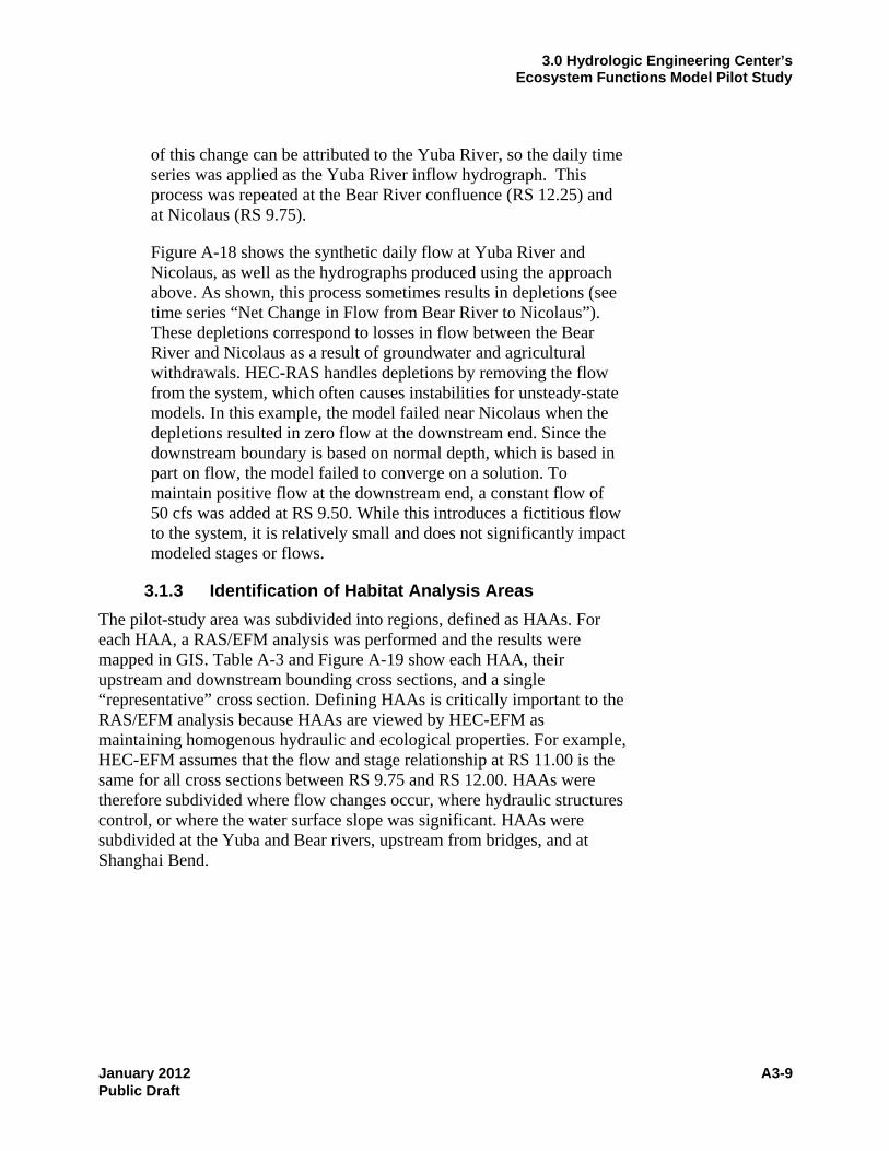
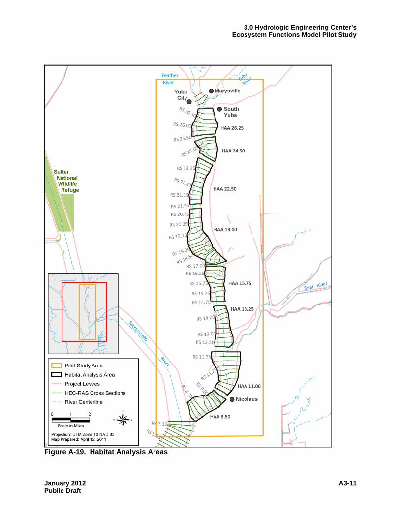
3.1.3 Identification of Habitat Analysis Areas The pilot-study area was subdivided into regions, defined as HAAs. For each HAA, a RAS/EFM analysis was performed and the results were mapped in GIS. Table A-3 and Figure A-19 show each HAA, their upstream and downstream bounding cross sections, and a single “representative” cross section. Defining HAAs is critically important to the RAS/EFM analysis because HAAs are viewed by HEC-EFM as maintaining homogenous hydraulic and ecological properties. For example, HEC-EFM assumes that the flow and stage relationship at RS 11.00 is the same for all cross sections between RS 9.75 and RS 12.00. HAAs were therefore subdivided where flow changes occur, where hydraulic structures control, or where the water surface slope was significant. HAAs were subdivided at the Yuba and Bear rivers, upstream from bridges, and at Shanghai Bend.
2012 Central Valley Flood Protection Plan Attachment 9F: Floodplain Restoration Opportunity Analysis Appendix A. Floodplain Inundation and Ecosystem Functions Model Pilot Studies
A3-10 January 2012 Public Draft
-5,000
5,000
15,000
25,000
35,000
45,000
55,000
Oct 99 May 00 Nov 00 Jun 01 Dec 01 Jul 02 Jan 03 Aug 03
Daily
Flo
ws (
cfs)
Date
Total Flow at Yuba CityTotal Flow at NicolausNet Change in Flow from Yuba City to Yuba RiverNet Change in Flow from Yuba River to Bear RiverNet Change in Flow from Bear River to Nicolaus
Figure A-18. Revised Daily Flow Time Series Hydrographs
Table A-3. Habitat Analysis Areas
Bounding Cross Sections
Representative Cross Sections
7.55–9.50 8.50
9.75–12.00 11.00
12.25–14.50 13.25
14.75–16.75 15.75
17.00–21.00 19.00
21.25–23.75 22.50
24.00–25.25 24.50
25.50–27.00 26.25 Source: Data generated by AECOM for this report in 2011
3.0 Hydrologic Engineering Center’s Ecosystem Functions Model Pilot Study
January 2012 A3-11 Public Draft
Figure A-19. Habitat Analysis Areas
2012 Central Valley Flood Protection Plan Attachment 9F: Floodplain Restoration Opportunity Analysis Appendix A. Floodplain Inundation and Ecosystem Functions Model Pilot Studies
A3-12 January 2012 Public Draft
3.1.4 HEC-RAS Modeling Once HAAs were identified, the HEC-RAS unsteady-state model was used to produce synthetic stage and flow hydrographs at each representative cross section. These hydrographs were stored in a HEC Data Storage System (HEC-DSS) format database and used as input to HEC-EFM. In addition, a series of steady-state flow profiles was simulated to produce rating curves at each representative cross section. These rating curves were then used during the HEC-EFM modeling, as discussed in the following section.
3.1.5 HEC-EFM Modeling The HEC-EFM portion of the RAS/EFM analysis consisted of analyzing synthetic stage and flow hydrographs produced by HEC-RAS to determine if and when HEC-EFM Ecosystem Function Relationship (EFR) conditions were met. These conditions, defined by the user, include seasonality, duration, rate of change, and/or return frequency as a function of stage and flow.
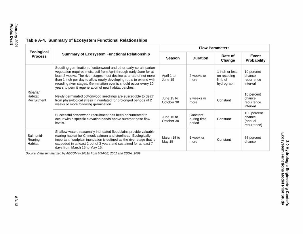
Using the stage and flow hydrographs developed by the HEC-RAS unsteady-state model, a HEC-EFM “flow regime” was created for each HAA. These flow regimes identify the flow and stage hydrographs that correspond to each HAA. EFRs were obtained from Table 3 in the September 2010 draft of 2012 Central Valley Flood Protection Plan—Ecosystem Functions Model (AECOM, 2010b). A summary of each EFR, directly from the above report, is provided in Table A-4. The EFRs used in this study included Salmonid-Rearing Habitat Formation, riparian Cottonwood Seedling Germination, riparian Cottonwood Seedling Inundation (death), and riparian Cottonwood Recruitment. Each EFR was added to HEC-EFM and is shown on Figures F-1 through F-4 in Appendix D-6F.
HEC-EFM was then used to analyze each EFR and HAA. HEC-EFM first performs a statistical analysis on each stage and flow hydrograph for each EFR to determine if and when conditions of the EFRs are met. During this analysis, HEC-EFM produces a stage-flow rating curve for each flow regime based on a statistical sampling of the stage and flow hydrographs. If conditions of the EFR are met, the flow or stage that meets the conditions is then used in conjunction with the rating curve to determine the corresponding flow or stage.
3.0 H
ydrologic Engineering Center’s
Ecosystem Functions M
odel Pilot Study
January 2021 A
3-13 Public D
raft
Table A-4. Summary of Ecosystem Functional Relationships
Ecological Process Summary of Ecosystem Functional Relationship
Flow Parameters
Season Duration Rate of Change
Event Probability
Riparian Habitat Recruitment
Seedling germination of cottonwood and other early-seral riparian vegetation requires moist soil from April through early June for at least 2 weeks. The river stages must decline at a rate of not more than 1 inch per day to allow newly developing roots to extend with receding river stages. Germination events should occur every 10 years to permit regeneration of new habitat patches.
April 1 to June 15
2 weeks or more
1 inch or less on receding limb of hydrograph
10 percent chance recurrence interval
Newly germinated cottonwood seedlings are susceptible to death from physiological stress if inundated for prolonged periods of 2 weeks or more following germination.
June 15 to October 30
2 weeks or more Constant
10 percent chance recurrence interval
Successful cottonwood recruitment has been documented to occur within specific elevation bands above summer base flow levels.
June 15 to October 30
Constant during time period
Constant
100 percent chance (annual recurrence)
Salmonid-Rearing Habitat
Shallow-water, seasonally inundated floodplains provide valuable rearing habitat for Chinook salmon and steelhead. Ecologically important floodplain inundation is defined as the river stage that is exceeded in at least 2 out of 3 years and sustained for at least 7 days from March 15 to May 15.
March 15 to May 15
1 week or more Constant 66 percent
chance
Source: Data summarized by AECOM in 2011b from USACE, 2002 and ESSA, 2009
2012 Central Valley Flood Protection Plan Attachment 9F: Floodplain Restoration Opportunity Analysis Appendix A. Floodplain Inundation and Ecosystem Functions Model Pilot Studies
A3-14 January 2012 Public Draft
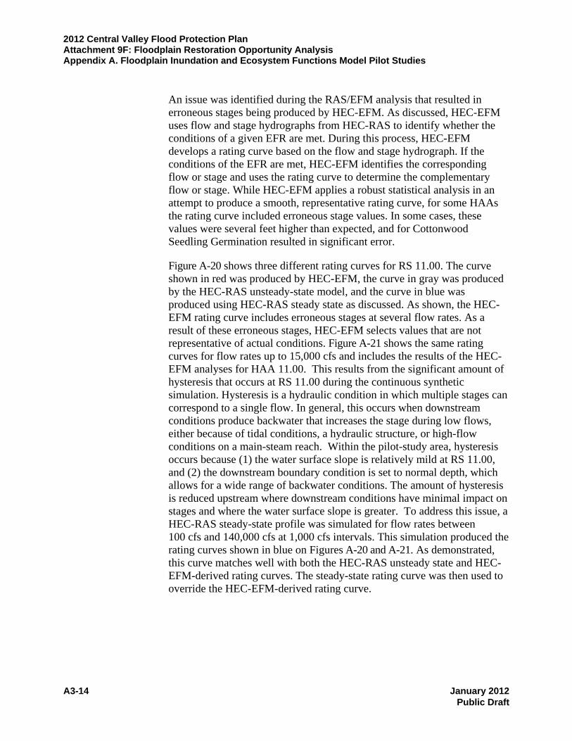
An issue was identified during the RAS/EFM analysis that resulted in erroneous stages being produced by HEC-EFM. As discussed, HEC-EFM uses flow and stage hydrographs from HEC-RAS to identify whether the conditions of a given EFR are met. During this process, HEC-EFM develops a rating curve based on the flow and stage hydrograph. If the conditions of the EFR are met, HEC-EFM identifies the corresponding flow or stage and uses the rating curve to determine the complementary flow or stage. While HEC-EFM applies a robust statistical analysis in an attempt to produce a smooth, representative rating curve, for some HAAs the rating curve included erroneous stage values. In some cases, these values were several feet higher than expected, and for Cottonwood Seedling Germination resulted in significant error.
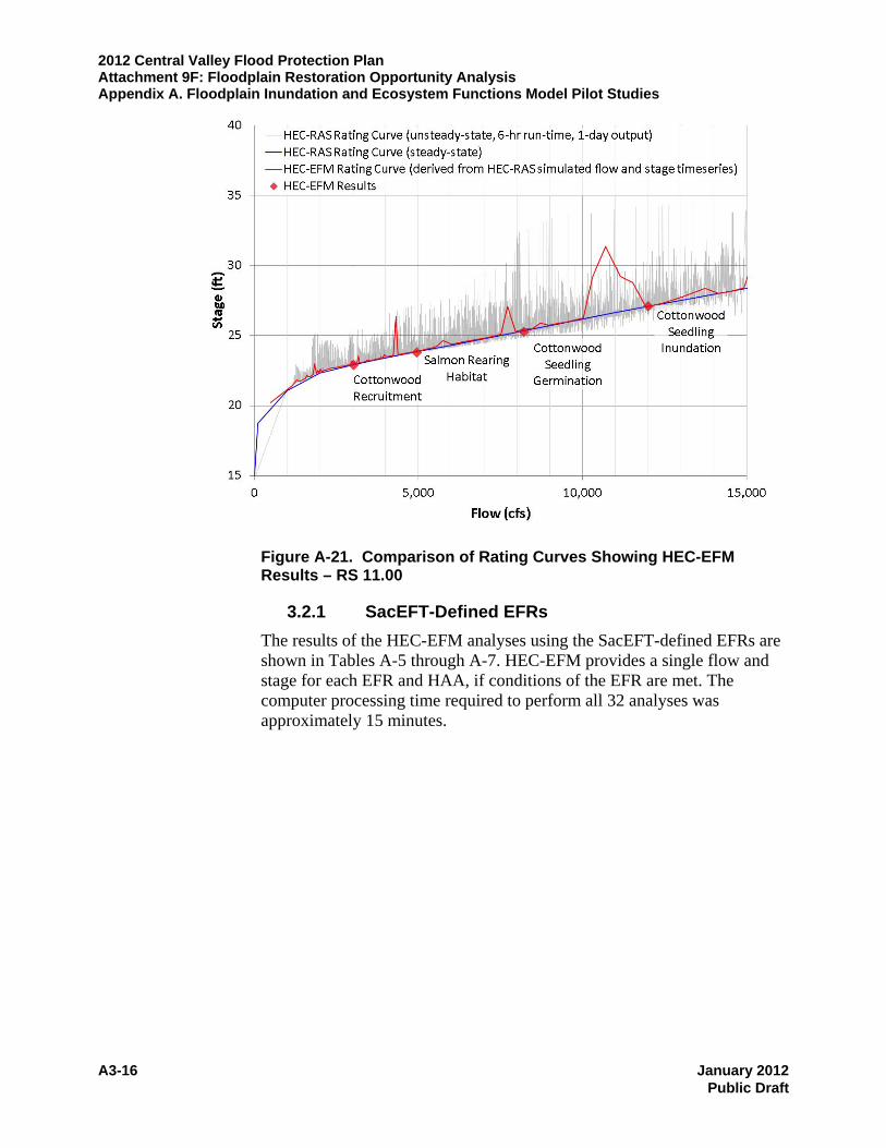
Figure A-20 shows three different rating curves for RS 11.00. The curve shown in red was produced by HEC-EFM, the curve in gray was produced by the HEC-RAS unsteady-state model, and the curve in blue was produced using HEC-RAS steady state as discussed. As shown, the HEC-EFM rating curve includes erroneous stages at several flow rates. As a result of these erroneous stages, HEC-EFM selects values that are not representative of actual conditions. Figure A-21 shows the same rating curves for flow rates up to 15,000 cfs and includes the results of the HEC-EFM analyses for HAA 11.00. This results from the significant amount of hysteresis that occurs at RS 11.00 during the continuous synthetic simulation. Hysteresis is a hydraulic condition in which multiple stages can correspond to a single flow. In general, this occurs when downstream conditions produce backwater that increases the stage during low flows, either because of tidal conditions, a hydraulic structure, or high-flow conditions on a main-steam reach. Within the pilot-study area, hysteresis occurs because (1) the water surface slope is relatively mild at RS 11.00, and (2) the downstream boundary condition is set to normal depth, which allows for a wide range of backwater conditions. The amount of hysteresis is reduced upstream where downstream conditions have minimal impact on stages and where the water surface slope is greater. To address this issue, a HEC-RAS steady-state profile was simulated for flow rates between 100 cfs and 140,000 cfs at 1,000 cfs intervals. This simulation produced the rating curves shown in blue on Figures A-20 and A-21. As demonstrated, this curve matches well with both the HEC-RAS unsteady state and HEC-EFM-derived rating curves. The steady-state rating curve was then used to override the HEC-EFM-derived rating curve.
3.0 Hydrologic Engineering Center’s Ecosystem Functions Model Pilot Study
January 2012 A3-15 Public Draft
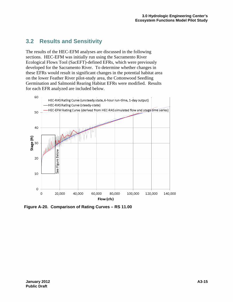
3.2 Results and Sensitivity
The results of the HEC-EFM analyses are discussed in the following sections. HEC-EFM was initially run using the Sacramento River Ecological Flows Tool (SacEFT)-defined EFRs, which were previously developed for the Sacramento River. To determine whether changes in these EFRs would result in significant changes in the potential habitat area on the lower Feather River pilot-study area, the Cottonwood Seedling Germination and Salmonid Rearing Habitat EFRs were modified. Results for each EFR analyzed are included below.
Figure A-20. Comparison of Rating Curves – RS 11.00
2012 Central Valley Flood Protection Plan Attachment 9F: Floodplain Restoration Opportunity Analysis Appendix A. Floodplain Inundation and Ecosystem Functions Model Pilot Studies
A3-16 January 2012 Public Draft
Figure A-21. Comparison of Rating Curves Showing HEC-EFM Results – RS 11.00
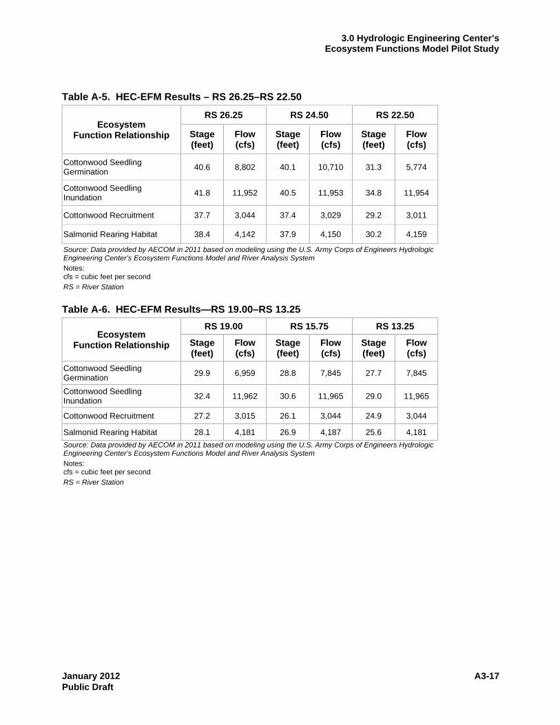
3.2.1 SacEFT-Defined EFRs The results of the HEC-EFM analyses using the SacEFT-defined EFRs are shown in Tables A-5 through A-7. HEC-EFM provides a single flow and stage for each EFR and HAA, if conditions of the EFR are met. The computer processing time required to perform all 32 analyses was approximately 15 minutes.
3.0 Hydrologic Engineering Center’s Ecosystem Functions Model Pilot Study
January 2012 A3-17 Public Draft
Table A-5. HEC-EFM Results – RS 26.25–RS 22.50
Ecosystem Function Relationship
RS 26.25 RS 24.50 RS 22.50
Stage (feet)
Flow (cfs)
Stage (feet)
Flow (cfs)
Stage (feet)
Flow (cfs)
Cottonwood Seedling Germination 40.6 8,802 40.1 10,710 31.3 5,774
Cottonwood Seedling Inundation 41.8 11,952 40.5 11,953 34.8 11,954
Cottonwood Recruitment 37.7 3,044 37.4 3,029 29.2 3,011
Salmonid Rearing Habitat 38.4 4,142 37.9 4,150 30.2 4,159
Source: Data provided by AECOM in 2011 based on modeling using the U.S. Army Corps of Engineers Hydrologic Engineering Center’s Ecosystem Functions Model and River Analysis System Notes: cfs = cubic feet per second RS = River Station
Table A-6. HEC-EFM Results—RS 19.00–RS 13.25
Ecosystem Function Relationship
RS 19.00 RS 15.75 RS 13.25
Stage (feet)
Flow (cfs)
Stage (feet)
Flow (cfs)
Stage (feet)
Flow (cfs)
Cottonwood Seedling Germination 29.9 6,959 28.8 7,845 27.7 7,845
Cottonwood Seedling Inundation 32.4 11,962 30.6 11,965 29.0 11,965
Cottonwood Recruitment 27.2 3,015 26.1 3,044 24.9 3,044
Salmonid Rearing Habitat 28.1 4,181 26.9 4,187 25.6 4,181 Source: Data provided by AECOM in 2011 based on modeling using the U.S. Army Corps of Engineers Hydrologic Engineering Center’s Ecosystem Functions Model and River Analysis System Notes: cfs = cubic feet per second RS = River Station
2012 Central Valley Flood Protection Plan Attachment 9F: Floodplain Restoration Opportunity Analysis Appendix A. Floodplain Inundation and Ecosystem Functions Model Pilot Studies
A3-18 January 2012 Public Draft
Table A-7. HEC-EFM Results—RS 11.00–RS 8.50
Ecosystem Function Relationship
RS 11.00 RS 8.50
Stage (feet)
Flow (cfs)
Stage (feet)
Flow (cfs)
Cottonwood Seedling Germination 25.3 8,198 23.1 7,635 Cottonwood Seedling Inundation 27.1 11,987 25.6 12,316 Cottonwood Recruitment 22.9 3,015 19.1 2,567 Salmonid Rearing Habitat 23.8 4,942 21.8 5,684 Source: Data provided by AECOM in 2011 based on modeling using the U.S. Army Corps of Engineers Hydrologic Engineering Center’s Ecosystem Functions Model and River Analysis System Notes: cfs = cubic feet per second RS = River Station
3.2.2 Modified EFRs The Cottonwood Seedling Germination and Salmonid Rearing Habitat Formation EFRs were modified to determine whether adjustments to the EFRs would result in significant changes in potential habitat area.
The Cottonwood Seedling Germination EFR Rate of Change of Stage (falling stage) statistical parameter was modified from the SacEFT-defined 1 inch per day to 2 inches per day and 3 inches per day. Also considered was a 1-inch-per-day Rate of Change of Stage from March to July, as opposed to the April to June 15 Sac-EFT-defined values. Lastly, the Rate of Change of Stage parameter was removed and instead germination was analyzed based on the 14-day minimum/maximum parameter (similar to the Cottonwood Seedling Inundation). Tables A-8 through A-10 show the results of these changes.
Table A-8. Cottonwood Seedling Germination Sensitivity – RS 26.25–RS 22.50
Ecosystem Function Relationship
RS 26.25 RS 24.50 RS 22.50
Stage (feet)
Flow (cfs)
Stage (feet)
Flow (cfs)
Stage (feet)
Flow (cfs)
1 inch per day 40.6 8,802 40.1 10,710 31.3 5,774 2 inches per day 42.7 14,242 41.3 15,182 35.0 12,395 3 inches per day 42.1 12,587 40.9 13,504 34.3 10,861 March - July 40.4 8,411 40.2 10,909 31.9 6,634 14-day Minimum/Maximum (no Rate of Change)
44.5 19,757 42.4 19,759 38.1 19,760
Source: Data provided by AECOM in 2011 based on modeling using the U.S. Army Corps of Engineers Hydrologic Engineering Center’s Ecosystem Functions Model and River Analysis System Notes: cfs = cubic feet per second RS = River Station
3.0 Hydrologic Engineering Center’s Ecosystem Functions Model Pilot Study
January 2012 A3-19 Public Draft
Table A-9. Cottonwood Seedling Germination Sensitivity – RS 19.00–RS 13.25
Ecosystem Function Relationship
RS 19.00 RS 15.75 RS 13.25
Stage (feet)
Flow (cfs)
Stage (feet)
Flow (cfs)
Stage (feet)
Flow (cfs)
1 inch per day 29.9 6,959 28.8 7,845 27.7 7,845 2 inches per day 33.1 13,680 31.6 14,361 29.9 14,394 3 inches per day 31.9 10,922 30.2 10,972 28.8 11,598 March - July 30.1 7,407 28.7 7,681 27.5 8,489 14-day Minimum/Maximum (no Rate of Change)
35.5 19,763 33.5 19,764 31.7 19,763
Source: Data provided by AECOM in 2011 based on modeling using the U.S. Army Corps of Engineers Hydrologic Engineering Center’s Ecosystem Functions Model and River Analysis System Notes: cfs = cubic feet per second RS = River Station
Table A-10. Cottonwood Seedling Germination Sensitivity – RS 11.00–RS 8.50
Ecosystem Function Relationship
RS 11.00 RS 8.50
Stage (feet)
Flow (cfs)
Stage (feet)
Flow (cfs)
1 inch per day 25.3 8,198 23.1 7,635 2 inches per day 28.4 15,074 27.0 15,429 3 inches per day 26.9 11,562 25.1 11,343 March - July 25.6 8,830 23.1 7,756 14-day Minimum/Maximum (no Rate of Change)
30.8 21,427 30.6 24,908
Source: Data provided by AECOM in 2011 based on modeling using the U.S. Army Corps of Engineers Hydrologic Engineering Center’s Ecosystem Functions Model and River Analysis System Notes cfs = cubic feet per second RS = River Station
2012 Central Valley Flood Protection Plan Attachment 9F: Floodplain Restoration Opportunity Analysis Appendix A. Floodplain Inundation and Ecosystem Functions Model Pilot Studies
A3-20 January 2012 Public Draft
The following can be concluded:
1. There appears to be an “optimum” Rate of Change of Stage value that corresponds to a maximum flow and stage and thus maximum potential habitat area. If this optimum Rate of Change of Stage value is considered ecologically “acceptable” (i.e., it still provides viable habitat given the greater rate of change) then it could be used to map the maximum potential habitat area.
2. Extending the analysis period did not significantly impact flows or stages. While extending the analysis period did not impact flows or changes on the lower Feather River, results may vary depending on the operational characteristics of upstream controls (e.g., dams) and therefore may vary depending on the stream reach.
3. Using a 14-day minimum/maximum query, as opposed to the Rate of Change of Stage, significantly increased flow and stage, resulting in greater potential habitat area. Consideration should be given as to the importance of the Rate of Change of Stage query since it significantly reduces the flow and stage and thus potential habitat area.
4. When assuming a 2-inch rate of change of stage or when removing the rate of change of stage criteria and using a 14-day minimum/maximum criteria, Cottonwood Seedling Germination produces higher flows and stages than Cottonwood Seedling Inundation. This suggests that successful Cottonwood recruitment may be possible under alternative EFR criteria. It should be noted, however, that Cottonwood Seedling Germination and Inundation are not dynamically linked with HEC-EFM and that any conclusions regarding recruitment success must be considered with this in mind.
The Salmonid Rearing Habitat Formation EFR was modified from the SacEFT-defined March through May, 7-day minimum/maximum and 67 percent chance frequency criteria to analyze various frequencies, including 50, 33, 20, and 10 percent chance, a 14-day duration and no duration criteria, and a 7-day duration from March through July. Tables A-11 through A-13 show the results of these changes.
3.0 Hydrologic Engineering Center’s Ecosystem Functions Model Pilot Study
January 2012 A3-21 Public Draft
The following can be concluded:
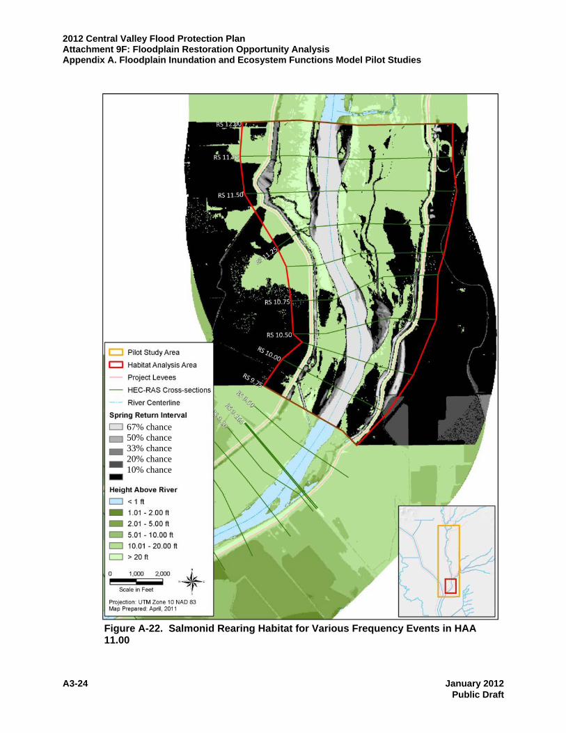
1. Flow and stage increase linearly with frequency. As expected, lower frequency criteria resulted in greater flow and stage. Figure A-22 shows the corresponding area for each 7-day duration frequency within HAA 11.00. Although the 10 percent chance frequency produces the greatest area (note: the 10 percent chance area includes all areas mapped under the 20 percent chance area, the 20 percent chance area includes all areas mapped under the 33 percent chance area, etc.), much of the area may not correspond to ideal salmonid habitat, given that successful salmonid habitat does not rely as heavily on widespread floodplain inundation but rather habitat located within side channels and along river banks.
2. Extending the period of the analysis to include June and July significantly increases the flow by 2 to 3 times. Unlike Cottonwood Seedling Germination, increasing the period of analysis results in greater potential habitat area. If June and July were considered ecologically “acceptable” periods for salmonid rearing, the period of analysis could be extended to increase the potential habitat area.
3. Removing the duration criteria increased the flow and stage minimally, while assuming 14-day duration versus 7-day duration minimally decreased the flow and stage. Adjusting the duration of the event did not significantly impact flows, stages, or potential habitat area.
2012 Central Valley Flood Protection Plan Attachment 9F: Floodplain Restoration Opportunity Analysis Appendix A. Floodplain Inundation and Ecosystem Functions Model Pilot Studies
A3-22 January 2012 Public Draft
Table A-11. Salmonid Rearing Habitat Sensitivity – RS 26.25–RS 22.50
Ecosystem Function Relationship
RS 26.25 RS 24.50 RS 22.50
Stage (feet)
Flow (cfs)
Stage (feet)
Flow (cfs)
Stage (feet)
Flow (cfs)
67% chance, 7-day duration 38.4 4,142 37.9 4,150 30.2 4,159 50% chance, 7-day duration 39.4 6,231 38.7 6,231 31.7 6,231 33% chance, 7-day duration 41.4 10,901 40.2 10,904 34.3 10,916 20% chance, 7-day duration 43.2 15,673 41.4 15,684 36.5 15,693 10% chance, 7-day duration 47.1 28,466 44.8 28,465 41.1 28,462 67% chance, 7-day duration March-July
41.6 11,265 40.3 11,232 34.4 11,200
67% chance; no duration 39.1 5,661 38.5 5,659 31.3 5,657 67% chance; 14-day duration 38.1 3,733 37.7 3,734 29.8 3,735 Source: Data provided by AECOM in 2011 based on modeling using the U.S. Army Corps of Engineers Hydrologic Engineering Center’s Ecosystem Functions Model and River Analysis System
Notes: cfs = cubic feet per second RS = River Station
Table A-12. Salmonid Rearing Habitat Sensitivity – RS 19.00–RS 13.25
Ecosystem Function Relationship
RS 19.00 RS 15.75 RS 13.25
Stage (feet)
Flow (cfs)
Stage (feet)
Flow (cfs)
Stage (feet)
Flow (cfs)
67% chance, 7-day duration 28.1 4,181 26.9 4,187 25.6 4,181 50% chance, 7-day duration 29.4 6,229 28.0 6,226 26.5 6,219 33% chance, 7-day duration 31.9 10,916 30.2 10,923 28.5 10,931 20% chance, 7-day duration 34.0 15,715 32.1 15,734 30.4 15,756 10% chance, 7-day duration 38.5 28,452 36.2 28,446 24.5 28,445 67% chance, 7-day duration March-July 32.0 11,121 30.2 11,060 28.5 11,031
67% chance; no duration 29.1 5,699 27.7 5,619 26.2 5,582 67% chance; 14-day duration 27.8 3,737 26.6 3,748 25.3 3,758 Source: Data provided by AECOM in 2011 based on modeling using the U.S. Army Corps of Engineers Hydrologic Engineering Center’s Ecosystem Functions Model and River Analysis System
Notes: cfs = cubic feet per second RS = River Station
3.0 Hydrologic Engineering Center’s Ecosystem Functions Model Pilot Study
January 2012 A3-23 Public Draft
Table A-13. Salmonid Rearing Habitat Sensitivity – RS 11.00–RS 8.50
Ecosystem Function Relationship
RS 11.00 RS 8.50
Stage (feet)
Flow (cfs)
Stage (feet)
Flow (cfs)
67% chance, 7-day Duration 23.8 4,942 21.8 5,684 50% chance, 7-day Duration 25.0 7,536 24.3 9,762 33% chance, 7-day Duration 27.0 11,832 27.1 15,760 20% chance, 7-day Duration 29.1 16,800 29.3 21,232 10% chance, 7-day Duration 34.4 32,453 34.7 38,506 67% chance, 7-day Duration March-July 26.7 11,175 24.7 10,592
67% chance; No Duration 24.7 6,706 23.0 7,443 67% chance; 14-day Duration 23.4 3,999 21.4 5,079 Source: Data provided by AECOM in 2011 based on modeling using the U.S. Army Corps of Engineers Hydrologic Engineering Center’s Ecosystem Functions Model and River Analysis System
Notes: cfs = cubic feet per second RS = River Station
3.3 Mapping
This section includes the results of the HEC-EFM analysis and the use of various mapping approaches to spatially visualize the HEC-EFM results. It also includes a discussion of how the spatial results can be further refined and reviewed to identify potential alternatives and how the final results can be presented.
3.3.1 Mapping Approaches While HEC-EFM provides a stage and flow that meets the conditions of a given EFR, additional efforts are required to visualize the spatial area along the river that meets those conditions. Three approaches to mapping the results of HEC-EFM are presented in the following sections.
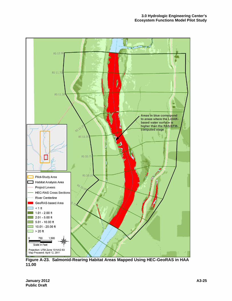
HEC-GeoRAS The HEC-EFM results discussed above were mapped using HEC-RAS and the GIS extension to HEC’s River Analysis System (HEC-GeoRAS), as recommended in the USACE-HEC HEC-EFM Quick Start Guide (USACE-HEC, 2009 (see Figure A-23)). This approach uses the flow rates determined by HEC-EFM but disregards the stages determined by HEC-EFM.
2012 Central Valley Flood Protection Plan Attachment 9F: Floodplain Restoration Opportunity Analysis Appendix A. Floodplain Inundation and Ecosystem Functions Model Pilot Studies
A3-24 January 2012 Public Draft
Figure A-22. Salmonid Rearing Habitat for Various Frequency Events in HAA 11.00
67% chance 50% chance 33% chance 20% chance 10% chance
3.0 Hydrologic Engineering Center’s Ecosystem Functions Model Pilot Study
January 2012 A3-25 Public Draft
Figure A-23. Salmonid-Rearing Habitat Areas Mapped Using HEC-GeoRAS in HAA 11.00
2012 Central Valley Flood Protection Plan Attachment 9F: Floodplain Restoration Opportunity Analysis Appendix A. Floodplain Inundation and Ecosystem Functions Model Pilot Studies
A3-26 January 2012 Public Draft
The flow rates determined by HEC-EFM at each representative cross section were used as input for the HEC-RAS steady-state model. HEC-RAS was then used to compute the water-surface profiles for each HAA that corresponded to the flow determined by HEC-EFM. The entire pilot-study area HEC-RAS model was used to analyze each HAA (i.e., the model was not truncated to each HAA). This was done to maintain proper upstream and downstream boundary conditions and because truncating the model to each HAA would not necessarily reduce and could likely increase the level of effort.
The water-surface profile for each HAA and EFR were then mapped using the HEC-GeoRAS tool within ArcGIS. The water surface areas correspond to areas that meet the EFR conditions, as determined by HEC-EFM and HEC-RAS. It took approximately 10 minutes of processing time to run the HEC-GeoRAS tool for a single HAA and EFR. Each water surface area polygon was then clipped to its respective HAA. It should be noted that the inundation depth grid, a product of HEC-GeoRAS that is used in the HEC-EFM manual to show the extent of potential habitat, is not shown. The depth grid was not shown because the water surface area polygon is simpler for readers to identify with and is easier to work with in ArcGIS. Results are shown on Figures G-1 through G-11 in Appendix D-6G for each HAA and EFR (Cottonwood Recruitment was not mapped because potential habitat areas outside of the channel banks were not identified). The background of each map corresponds to the LiDAR-based FIP.
The following are important findings of this approach:
1. The water surface areas mapped are the direct, raw product of the RAS/EFM analysis. Areas have not been refined based on additional ecological or biological considerations, such as soil type, vegetation type, bank slope, connectivity, or land use.
2. HEC-RAS and HEC-GeoRAS cannot map areas beyond the HEC-RAS model cross sections. As a result, areas beyond existing levees are not mapped. Cross sections would need to be extended beyond the levees to map areas outside the existing levee system.
3. EFRs that produce stages below the LiDAR observed water surface are not mapped by HEC-GeoRAS. When EFR stages are below the LiDAR-observed water surface, water surface area does exist; however, the area is simply below the LiDAR-
3.0 Hydrologic Engineering Center’s Ecosystem Functions Model Pilot Study
January 2012 A3-27 Public Draft
observed water surface. To resolve this issue, bathymetry would need to be combined with the LiDAR terrain.
Height Above River Although HEC-GeoRAS is a proven and reliable method for mapping HEC-RAS results, its limitation of mapping within cross-section extents makes it difficult to determine the potential for habitat beyond the existing levee system. Its inability to map below the LiDAR-observed water surface also reduces the value for mapping within channel banks. Thus, an alternative approach was reviewed using the FIP methodology.
After reviewing and testing the FIP approach as well as the HEC-GeoRAS and ArcGIS approaches, the FIP approach was selected as the preferred mapping approach.
Similar to the approach discussed above, HEC-RAS was used to simulate the water-surface profile for each HAA based on the flows determined by HEC-EFM. The results were exported to GIS, and HEC-GeoRAS was used to develop cross-section cut-lines with water surface elevations for each HAA and EFR. ArcGIS was then used to perform FIP analyses for each HAA and EFR. Figure A-24 shows an example of the Cottonwood Seedling Germination habitat area identified using the HEC-GeoRAS approach versus the FIP approach from RS 9.75 through RS 12.00 (HAA 11.00).
The following are important findings of this approach:
1. The FIP analysis is capable of mapping the RAS/EFM analysis results within the entire FIP study area. Mapping was not limited to the cross-section extents and provides mapping beyond the existing levee system.
2. The FIP analysis replaces the LiDAR-observed water surface with the water-surface profiles computed by HEC-RAS, based on predefined bank breaklines. As a result, the entire channel, from bank to bank, is shown as meeting the RAS/EFM analysis EFR criteria. This may overestimate the area of potential habitat within the channel. To resolve this issue, bathymetry would need to be combined with the LiDAR terrain.
3. The water surface areas mapped are the direct, raw product of the RAS/ EFM analysis. Areas have not been refined based on additional ecological or biological considerations, such as soil type, vegetation type, bank slope, connectivity, or land use.
2012 Central Valley Flood Protection Plan Attachment 9F: Floodplain Restoration Opportunity Analysis Appendix A. Floodplain Inundation and Ecosystem Functions Model Pilot Studies
A3-28 January 2012 Public Draft
ArcGIS The approaches discussed above use HEC-RAS to determine the water-surface profile within each HAA that meet the conditions of each EFR. These water-surface profiles are computed by HEC-RAS using the flows determined by HEC-EFM. While these approaches provide hydraulically correct water-surface profiles through each HAA, they require a significant level of effort. An alternative was considered using ArcGIS to directly map the stage determined by HEC-EFM. This approach uses the stage determined by HEC-EFM instead of the flow rate, with the stage mapped within ArcGIS for each HAA and EFR.
This approach assumes that the stage determined by HEC-EFM for a given HAA and EFR applies uniformly across the HAA (i.e., it assumes there is no slope to the water surface throughout the HAA). This assumption may or may not be valid, depending on the hydraulic characteristics of the HAA.
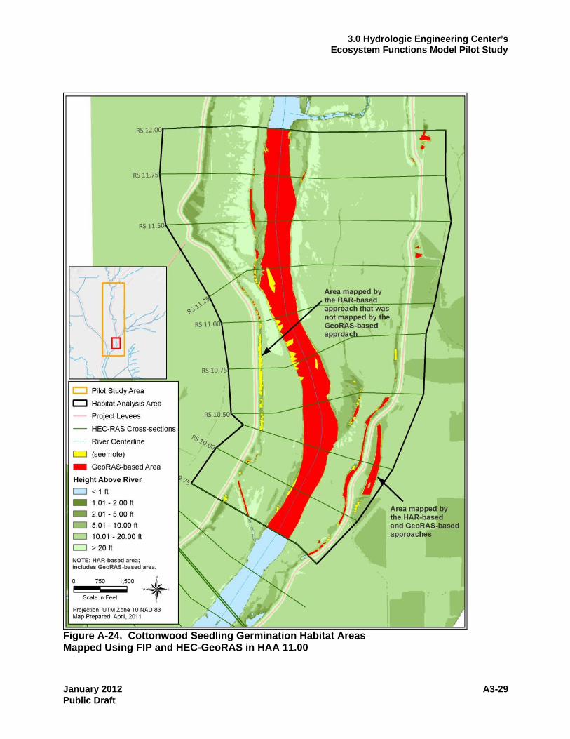
3.0 Hydrologic Engineering Center’s Ecosystem Functions Model Pilot Study
January 2012 A3-29 Public Draft
Figure A-24. Cottonwood Seedling Germination Habitat Areas Mapped Using FIP and HEC-GeoRAS in HAA 11.00
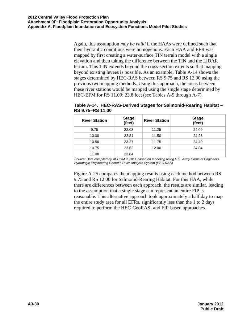
2012 Central Valley Flood Protection Plan Attachment 9F: Floodplain Restoration Opportunity Analysis Appendix A. Floodplain Inundation and Ecosystem Functions Model Pilot Studies
A3-30 January 2012 Public Draft
Again, this assumption may be valid if the HAAs were defined such that their hydraulic conditions were homogenous. Each HAA and EFR was mapped by first creating a water-surface TIN terrain model with a single elevation and then taking the difference between the TIN and the LiDAR terrain. This TIN extends beyond the cross-section extents so that mapping beyond existing levees is possible. As an example, Table A-14 shows the stages determined by HEC-RAS between RS 9.75 and RS 12.00 using the previous two mapping methods. Using this approach, the areas between these river stations would be mapped using the single stage determined by HEC-EFM for RS 11.00: 23.8 feet (see Tables A-5 through A-7).
Table A-14. HEC-RAS-Derived Stages for Salmonid-Rearing Habitat – RS 9.75–RS 11.00
River Station Stage (feet) River Station Stage
(feet) 9.75 22.03 11.25 24.09 10.00 22.31 11.50 24.25 10.50 23.27 11.75 24.40 10.75 23.62 12.00 24.84 11.00 23.84
Source: Data compiled by AECOM in 2011 based on modeling using U.S. Army Corps of Engineers Hydrologic Engineering Center’s River Analysis System (HEC-RAS)
Figure A-25 compares the mapping results using each method between RS 9.75 and RS 12.00 for Salmonid-Rearing Habitat. For this HAA, while there are differences between each approach, the results are similar, leading to the assumption that a single stage can represent an entire FIP is reasonable. This alternative approach took approximately a half day to map the entire study area for all EFRs, significantly less than the 1 to 2 days required to perform the HEC-GeoRAS- and FIP-based approaches.
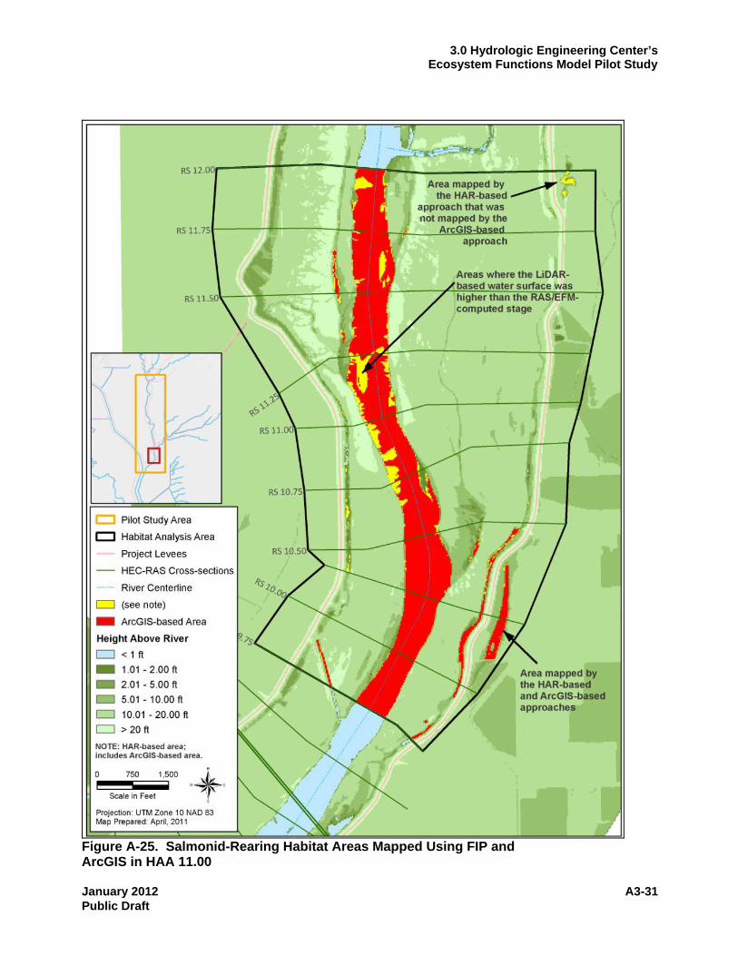
3.0 Hydrologic Engineering Center’s Ecosystem Functions Model Pilot Study
January 2012 A3-31 Public Draft
Figure A-25. Salmonid-Rearing Habitat Areas Mapped Using FIP and ArcGIS in HAA 11.00
2012 Central Valley Flood Protection Plan Attachment 9F: Floodplain Restoration Opportunity Analysis Appendix A. Floodplain Inundation and Ecosystem Functions Model Pilot Studies
A3-32 January 2012 Public Draft
The following are important findings of this approach:
1. Mapping stages directly from HEC-EFM may or may not be appropriate, depending on whether the HAA is hydraulically homogenous. For HAA 11.00, this approach provides a reasonable estimate of the area very similar to the FIP-based approach.
2. The water surface areas mapped are the direct, raw product of the RAS/EFM analysis. Areas have not been refined based on additional ecological or biological considerations, such as soil type, vegetation type, bank slope, connectivity, or land use.
3. EFRs that produce stages below the LiDAR-observed water surface are not mapped by ArcGIS. When EFR stages are below the LiDAR-observed water surface, water-surface area does exist; however, the area is simply below the LiDAR-observed water surface. To resolve this issue, bathymetry would need to be combined with the LiDAR terrain.
3.3.2 Refinement of Mapping Products Results of the mapping process can be further refined, quantified, and/or visualized in ArcGIS. For example, a series of spatial analyses could be conducted to calculate the area of potential habitat based on location, connected vs. disconnected (to the main channel), and/or the specific EFR. Other GIS layers, such as soils, known habitat areas, vegetation type, bank slope, connectivity, and depth, could be used to refine the mapping products and assist in identifying areas where alternatives may be used to create additional habitat.
3.4 Conclusions
The purpose of this pilot study was to understand the methods and approaches required for the HEC-RAS and HEC-EFM analysis and to identify any issues with or alternative approaches to the analysis. The intent of this study was not to develop a final restoration opportunities analysis for the lower Feather River. This report should serve to clarify the RAS/EFM analysis and to identify topics for discussion.
3.0 Hydrologic Engineering Center’s Ecosystem Functions Model Pilot Study
January 2012 A3-33 Public Draft
The following general conclusions were reached as a result of this pilot study:
1. While HEC-EFM is a robust tool for querying historic flow records, EFRs rely on a single set of numerical criteria (as opposed to a range) and lack dynamic (i.e., year-to-year) coupling of relationships. The project team and stakeholders expressed concern that a single EFR may not adequately identify potential habitat areas because the EFR defines areas based on a single set of numerical criteria, as opposed to a range. While these criteria may reflect optimal conditions for an ecological process, the ecological process may achieve some success at sub-optimal conditions. Multiple EFRs could be developed for a single ecological process representing “optimal,” “sub-optimal,” and “minimal” conditions; however, this would significantly increase the level of effort required for a systemwide analysis. As an alternative, a single EFR representing a broader range of conditions could be considered.
In addition, HEC-EFM does not dynamically couple EFRs. Since Cottonwood Seedling Recruitment relies on germination followed by minimal inundation within the same year, without dynamically coupling the two EFRs, the results are heavily skewed toward the relationship that produces the greater flow and stage.
2. The SacEFT HEC-EFM EFRs may not be applicable systemwide. The primary concern with using the SacEFT EFRs systemwide, as identified by project team members and Stakeholders, is that the existing EFRs were developed for the Sacramento River mainstem and may not be applicable to the Sacramento River tributaries and/or other rivers in the study area, such as the San Joaquin River and its tributaries.
3. The pilot study did not identify significant amounts of potential habitat on the lower Feather River and the RAS/EFM analysis would likely produce similar results systemwide. Because of the existing conditions of the lower Feather River and because of how EFRs are defined (as discussed above), limited habitat was identified on the lower Feather River. Given the conditions on other rivers within the project area (e.g., heavily leveed, restrained by dams, and/or incised), similar results may be produced systemwide.
Based on these conclusions, the project team considered developing a single EFR with a broader range of criteria, possibly with an upper- and lower-bound, to represent habitat opportunities. For example, the EFR may
2012 Central Valley Flood Protection Plan Attachment 9F: Floodplain Restoration Opportunity Analysis Appendix A. Floodplain Inundation and Ecosystem Functions Model Pilot Studies
A3-34 January 2012 Public Draft
represent the peak 50 percent chance flow that occurs during a 7-day duration spring and/or summer storm event. An upper and lower bound EFR may correspond to a higher or lower frequency and/or greater or smaller duration and/or time period. In combination with HEC-EFM and/or other statistical tools (e.g., the USACE HEC Statistical Software Package (HEC-SSP)), the synthetic flow record derived from the CalSim model may be queried at select locations where potential habitat is likely to exist. The EFR criteria will be based solely on flow, and since the CalSim-based flow records are developed wherever significant changes in flow occur, the development of HAAs is not critical. The flows associated with the EFR at these locations would then be mapped using HEC-RAS (steady-state) and the FIP approach. Regardless of whether HEC-EFM and/or other statistical tools, such as HEC-SSP, are used to query the flow records, it is the EFR criteria that ultimately determines the amount of potential habitat area identified. Therefore, the use of HEC-EFM versus other statistical tools should be based primarily on the ease of use, time required to set up, and output results from the software.

4.0 References
January 2012 A4-35 Public Draft
4.0 References

2012 Central Valley Flood Protection Plan Attachment 9F: Floodplain Restoration Opportunity Analysis Appendix A. Floodplain Inundation and Ecosystem Functions Model Pilot Studies
A4-36 January 2012 Public Draft
This page left blank intentionally.
5.0 Acronyms and Abbreviations
January 2012 A5-1 Public Draft
5.0 Acronyms and Abbreviations cfs .............................. cubic feet per second
Comprehensive Study Sacramento and San Joaquin River Basins Comprehensive Study
CVFED ...................... Central Valley Floodplain Evaluation and Delineation
CVP ........................... Central Valley Project
DEM .......................... digital elevation model
DWR .......................... California Department of Water Resources
EFR ........................... Ecosystem Function Relationship
ESRI .......................... Environmental Systems Research Institute, Inc.
FIP ............................. floodplain inundation potential
FROA ........................ Floodplain Restoration Opportunity Analysis
FTP ............................
GIS ............................ geographic information system
HAA ........................... Habitat Analysis Areas
HAR ........................... Height Above River
HEC-DSS .................. Hydrologic Engineering Center’s Data Storage System
HEC-EFM .................. Hydrologic Engineering Center’s Ecosystem Functions Model
HEC-GeoRAS ........... Hydrologic Engineering Center’s River Analysis System
HEC-RAS .................. Hydrologic Engineering Center’s River Analysis System
HEC-SSP .................. Hydrologic Engineering Center’S Statistical Software Package
LiDAR ........................ Light Detection and Ranging
MWH ......................... MWH Americas, Inc.
NAVD88 .................... North American Vertical Datum 1988
NGS ........................... National Geodetic Survey
NGVD29 .................... National Geodetic Vertical Datum of 1929
RAS/EFM .................. HEC-RAS/HEC-EFM
2012 Central Valley Flood Protection Plan Attachment 9F: Floodplain Restoration Opportunity Analysis Appendix A. Floodplain Inundation and Ecosystem Functions Model Pilot Studies
A5-2 January 2012 Public Draft
RS .............................. River Station
SacEFT ...................... Sacramento River Ecological Flows Tool
SWP .......................... State Water Project
TIN ............................. triangular irregular network
TM ............................. Technical Memorandum
UNET .........................
USACE ...................... U.S. Army Corps of Engineers
USGS ........................ U.S. Geological Survey
WSEL ........................ water surface elevations
WY ............................. Water Year
STATE OF CALIFORNIA THE NATURAL RESOURCES AGENCY DEPARTMENT OF WATER RESOURCES
Public Draft 2012 Central Valley Flood Protection Plan
Attachment 9F: Floodplain Restoration Opportunity Analysis – Appendix B. Investigation of USGS 10-Meter DEM Accuracy January 2012

January 2012 Public Draft
This page left blank intentionally.
Investigation of USGS 10-Meter DEM Accuracry
January 2012 B-1 Public Draft
U.S. Geological Survey (USGS) 10-meter digital elevation models (DEM) were obtained (USGS, 2010) and evaluated for their appropriateness of use in the pilot study along the lower Feather River. This appendix provides the methods and results of a brief assessment of these data.
A portion of the California Department of Water Resources Central Valley Flood Evaluation and Delineation Project (CVFED) light detection and ranging (LiDAR)-derived DEM was selected (see inset box on Figure B-1) and a cross section was taken of the levee to compare the elevations from both the USGS DEM and LiDAR-derived DEM.
Elevations in the vicinity of the levee cross section are shown on Figure B-2 from the LiDAR-derived DEM, and Figure B-3 from the USGS DEM, indicating a significant difference in the two data sets with the USGS data presenting essentially “flat” topography in this location.
Figure B-4 provides a profile view of the two cross sections, demonstrating the lack of topographic relief provided in the USGS DEM data, and Figure B-5 provides tabular data indicating a USGS DEM surface is approximately 6 feet higher landward from the levee.
Given this comparison of the USGS DEM against the LiDAR DEM, it was determined that the USGS data does not pick up the crests of project levees. In many cases, the USGS data barely show any increase in elevation at the levee crest, and present a higher ground elevation landward from the levee. Based on this comparison, it was determined that the USGS DEM cannot be used as a substitute for the LiDAR-derived DEM data.
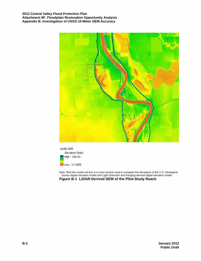
2012 Central Valley Flood Protection Plan Attachment 9F: Floodplain Restoration Opportunity Analysis Appendix B. Investigation of USGS 10-Meter DEM Accuracy
B-2 January 2012 Public Draft
Note: Red line inside red box is a cross section used to compare the elevations of the U.S. Geological Survey digital elevation model and Light Detection and Ranging-derived digital elevation model.
Figure B-1 LiDAR-Derived DEM of the Pilot-Study Reach
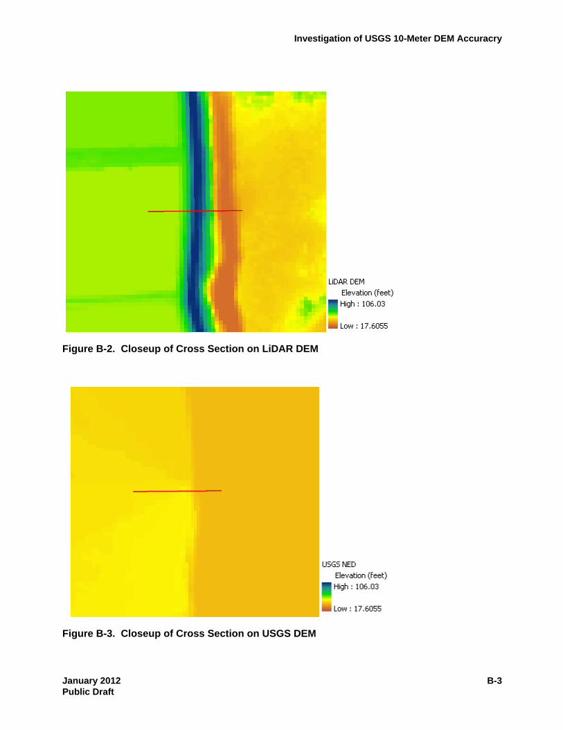
Investigation of USGS 10-Meter DEM Accuracry
January 2012 B-3 Public Draft
Figure B-2. Closeup of Cross Section on LiDAR DEM
Figure B-3. Closeup of Cross Section on USGS DEM
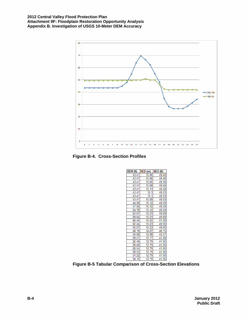
2012 Central Valley Flood Protection Plan Attachment 9F: Floodplain Restoration Opportunity Analysis Appendix B. Investigation of USGS 10-Meter DEM Accuracy
B-4 January 2012 Public Draft
Figure B-4. Cross-Section Profiles
Figure B-5 Tabular Comparison of Cross-Section Elevations
STATE OF CALIFORNIA THE NATURAL RESOURCES AGENCY DEPARTMENT OF WATER RESOURCES
Public Draft 2012 Central Valley Flood Protection Plan
Attachment 9F: Floodplain Restoration Opportunity Analysis – Appendix C. CVFED LiDAR Terrain Data Comparisons
January 2012

January 2012 Public Draft
This page left blank intentionally.
CVFED LiDAR Terrain Data Comparisons
January 2012 C-1 Public Draft
Since final digital elevation models (DEM) were not available from the California Department of Water Resources (DWR) Central Valley Flood Evaluation and Delineation Project (CVFED) program at the time of this pilot study, the DEM preparation involved the use of preliminary CVFED terrain data and incorporating/building breaklines and filling in void areas found in the data to create a triangulated irregular network (TIN) from which to derive a DEM of a specified grid cell size. An approximate 30- square-mile area was defined for the DEM preparation (Figure C-1). The light detection and ranging (LiDAR) data had data voids where there is water and dense vegetation that restricted the TIN from triangulating, essentially leaving large gaps in the TIN. Points were created in those areas to help complete the TIN.
Factors considered in the completion of the TIN and DEM included:
1. Projection – The were in a standard coordinate system; however, if they were not, then the LAS files would need to be converted to a shapefile and reprojected.
2. Data Voids – Where the data did not have interpolated points/breaklines across data void areas for the TIN to easily triangulate, “filler” points were created to provide a surface across the void areas to enable the completion of the TIN surface.
3. TIN/DEM Build – This process was iterative and required that no gaps remained in the TIN and resulting DEM. For every gap found, a search radius was applied to identify the nearest points to triangulate.
At the request of the Project Team, a comparison was made of the preparation time, resolution (usability), and file size attributes for various DEM grid size resolutions. This comparison included 5-, 25-, 50-, and 100-foot DEMs in the Feather River pilot-study area.
The time difference associated with DEM sampling from the TIN was minor. The time considerations came primarily from the initial TIN build (especially if the LiDAR has data voids) and this was estimated to take 2 to 3 days per 100 square miles. Another potentially significant impact on preparation time would be hydro-correction of the terrain surface; however, this was not done, which preserved the actual topographic condition of the floodplain surfaces.
A sample portion of the pilot-study area was prepared at the various DEM grid cell resolutions to enable a visual comparison of the resolution differences (Figures C-2 to C-5).
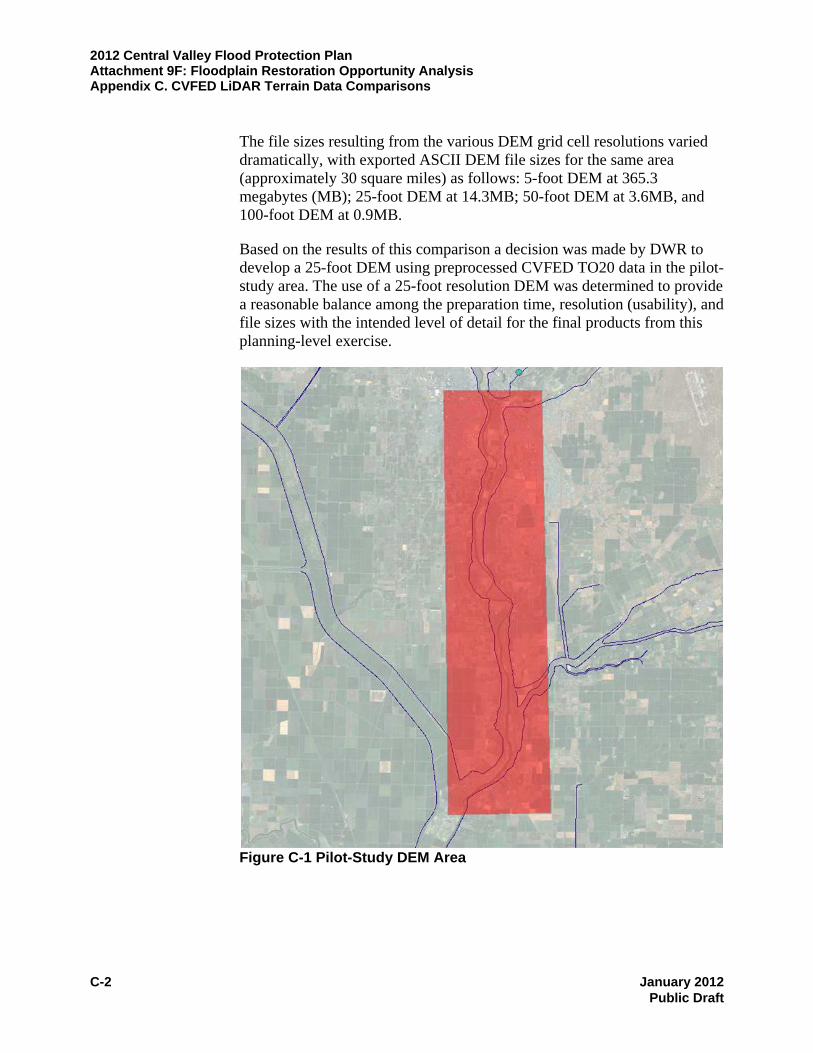
2012 Central Valley Flood Protection Plan Attachment 9F: Floodplain Restoration Opportunity Analysis Appendix C. CVFED LiDAR Terrain Data Comparisons
C-2 January 2012 Public Draft
The file sizes resulting from the various DEM grid cell resolutions varied dramatically, with exported ASCII DEM file sizes for the same area (approximately 30 square miles) as follows: 5-foot DEM at 365.3 megabytes (MB); 25-foot DEM at 14.3MB; 50-foot DEM at 3.6MB, and 100-foot DEM at 0.9MB.
Based on the results of this comparison a decision was made by DWR to develop a 25-foot DEM using preprocessed CVFED TO20 data in the pilot-study area. The use of a 25-foot resolution DEM was determined to provide a reasonable balance among the preparation time, resolution (usability), and file sizes with the intended level of detail for the final products from this planning-level exercise.
Figure C-1 Pilot-Study DEM Area
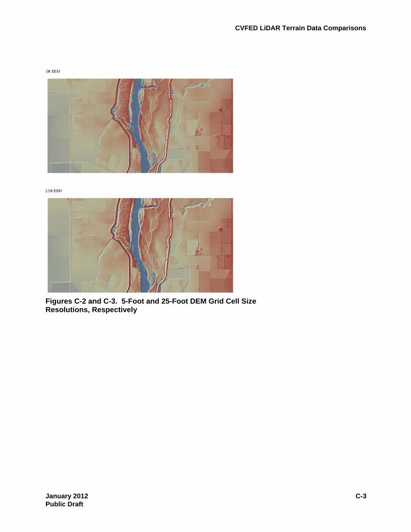
CVFED LiDAR Terrain Data Comparisons
January 2012 C-3 Public Draft
Figures C-2 and C-3. 5-Foot and 25-Foot DEM Grid Cell Size Resolutions, Respectively
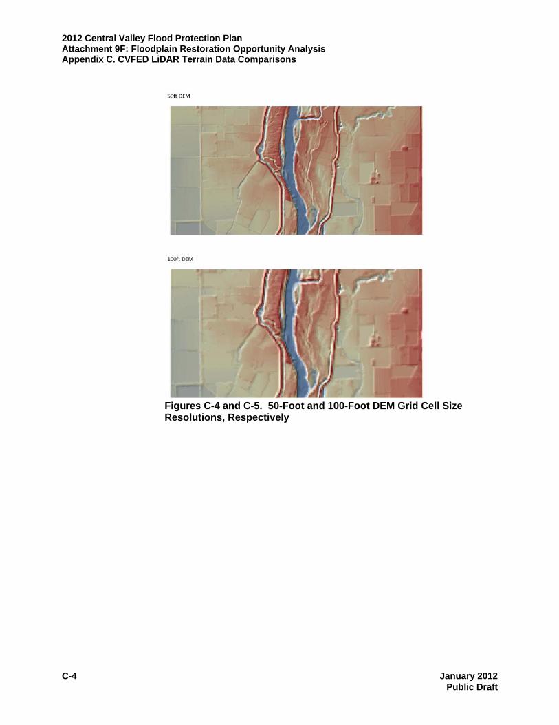
2012 Central Valley Flood Protection Plan Attachment 9F: Floodplain Restoration Opportunity Analysis Appendix C. CVFED LiDAR Terrain Data Comparisons
C-4 January 2012 Public Draft
Figures C-4 and C-5. 50-Foot and 100-Foot DEM Grid Cell Size Resolutions, Respectively

CVFED LiDAR Terrain Data Comparisons
January 2012 C-5 Public Draft
This page left blank intentionally.

STATE OF CALIFORNIA THE NATURAL RESOURCES AGENCY DEPARTMENT OF WATER RESOURCES
Public Draft 2012 Central Valley Flood Protection Plan
Attachment 9F: Floodplain Restoration Opportunity Analysis – Appendix D. Levee Realignment Methodology January 2012

January 2012 Public Draft
This page left blank intentionally.
Levee Realignment Methodology
January 2012 D-1 Public Draft
Within the Feather River pilot-study reach, the Project Team noted that there were two locations where levees had been set back since the March 2008 date of the light detection and ranging (LiDAR) flight. This resulted in a need to adjust the digital elevation model (DEM) terrain surface to show actual current topographic conditions. While the Height Above River (HAR) output to date still shows the old levee position, a separate effort was made to determine a reasonable approach to adjust levee locations for subsequent HAR analyses.
The following steps were taken to adjust the location of a levee in the DEM.
1. A polygon feature was created around the area of the existing and new levee locations. The polygon was used to clip the DEM, which cut down on the processing time (Figure D-1).
2. A copy of the DEM surface limited to the polygon area was extracted by using the Extract by Mask tool located in the ArcGIS Toolbox -> Spatial Analyst Tools -> Extraction -> Extract by Mask (Figures D-2 and Figure-D3, tool input Items a through c below; and Figure D-4, output resulting from Items a through c below).
a. Input Raster – Input the DEM.
b. Input Raster or Feature Mask Data – Input the polygon created in Step 1.
c. User must set file location and name.
3. The raster was converted into points using the 3D Analyst Toolbar dropdown menu under Convert -> Raster to Features (Figure D-5).
a. Output Geometry Type – Set to Point.
b. Input Raster – This is the extracted raster from Step 2.
c. Field – Set to <Value>.
d. User must set output file location and name.
4. The existing and new levees were delineated with lines that were then buffered at a distance necessary to capture the entire width of the levee cells in the DEM (Figure D-6).
5. All points within the buffered areas were selected by using Main Menu -> Selection -> Select by Location (Figures D-7 and D-8, tool input

2012 Central Valley Flood Protection Plan Attachment 9F: Floodplain Restoration Opportunity Analysis Appendix D. Levee Realignment Methodology
D-2 January 2012 Public Draft
Items a through d below; and Figures D-9 and D-10, output from Items a through d below).
a. I want to – Pull down “Select Features From.”
b. The Following Layer – Click on the points file output from Step 3.
c. That – Pull down “are within.”
d. The features in this layer – Pull down “New Levees Buffer” created from Step 4.
e. The DEM polygon points selected within the new levee buffer area were deleted and the DEM polygon points selected within the existing levee buffer were exported using Step 6 before being deleted.
6. The points for the existing levee were selected in Step 5 and then exported by right clicking on the file name in the Layers Catalog: File Name -> Data -> Export Data. (Figures D-11 and D-12, tool input Items a through c below).
a. Export – Pull down “Selected features.”
b. Use the same coordinate system as – Select “this layer’s source data.”
c. Output shapefile or feature class – User sets file location and name.
7. The existing levee points from Step 6 were moved into the location of the deleted new levee points (Step 5e) in the Raster to Features point output from Step 3. This was done from the upstream portion of the levee to the downstream portion, where points from the existing levee were selected in groups and manually moved into the vacant new levee location. Occasionally a group of points needed to be rotated to fit the new area and maintain a consistent levee slope and height (Figure D-13).
8. The existing and new levee point layers were appended (combined) by entering the ArcGIS Toolbox, clicking on the Index Tab at the bottom, typing “Append” into the “Type in key word to find:” box at the top, and selecting “Append (management)” (Figures D-14 and D-15, tool input Items a through c below). This combines the levee points from Step 3 (as modified in Step 5e) and the newly moved levee points from Step 7 into one file (Figure D-16).
Levee Realignment Methodology
January 2012 D-3 Public Draft
a. Input Datasets – Enter filename for newly moved points from Step 7.
b. Target Dataset – Enter filename for points from Step 3, which were modified in Step 5e.
c. Schema Type (optional) – Pull down “NO TEST.”
9. All levee points were converted into a raster grid using the Features to Raster: Spatial Analyst toolbar -> Covert -> Features to Raster. (Figures D-17 and D-18, tool input Items a through d below).
a. Input Features – Appended points file from Step 8.
b. Field – This was set to GRID_CODE in the dropdown box.
c. Output Cell Size – Should be set to the cell size of the DEM.
d. Output Raster – User sets the raster file location and name.
10. The output raster had “NoData” value cells in the location of the existing levee because those points are no longer there. The next step involved filling these NoData cells with adjacent elevations from the DEM to create a smooth surface where the existing levee used to be (Figure D-19). This was done using the Spatial Analyst toolbar -> Raster Calculator (Figure D-20). In the expression box the following expression was typed, focalmean ([output raster from Step 9], rectangle, 3, 3, data ) (Figure D-21). This expression assigns the NoData cells the Mean of the 3x3 area around them. This expression did not fill in all NoData cells on the first run, so the output of this expression was run through the raster calculator a second and third time until all NoData cells were given an elevation (Figure D-22).
11. The output raster from Step 10 was converted to Points using the same Raster to Features method as in Step 3 (Figure D-23).
12. The DEM was converted to Points using the same Raster to Features method as in Steps 3 and 11 (Figure D-24).
13. Points from the DEM points file, created in Step 12, were selected within the polygon created in Step 1, using Select by Location, which was done in Step 5 (Figure D-25). Once all points within the polygon were selected, they were deleted from the DEM points file from Step 12. The points from Step 11 were fit into the vacant area (Figure D-26).
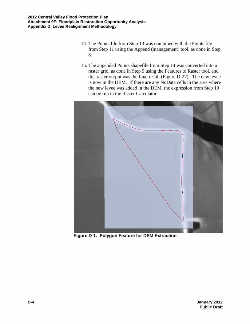
2012 Central Valley Flood Protection Plan Attachment 9F: Floodplain Restoration Opportunity Analysis Appendix D. Levee Realignment Methodology
D-4 January 2012 Public Draft
14. The Points file from Step 13 was combined with the Points file from Step 11 using the Append (management) tool, as done in Step 8.
15. The appended Points shapefile from Step 14 was converted into a raster grid, as done in Step 9 using the Features to Raster tool, and this raster output was the final result (Figure D-27). The new levee is now in the DEM. If there are any NoData cells in the area where the new levee was added in the DEM, the expression from Step 10 can be run in the Raster Calculator.
Figure D-1. Polygon Feature for DEM Extraction
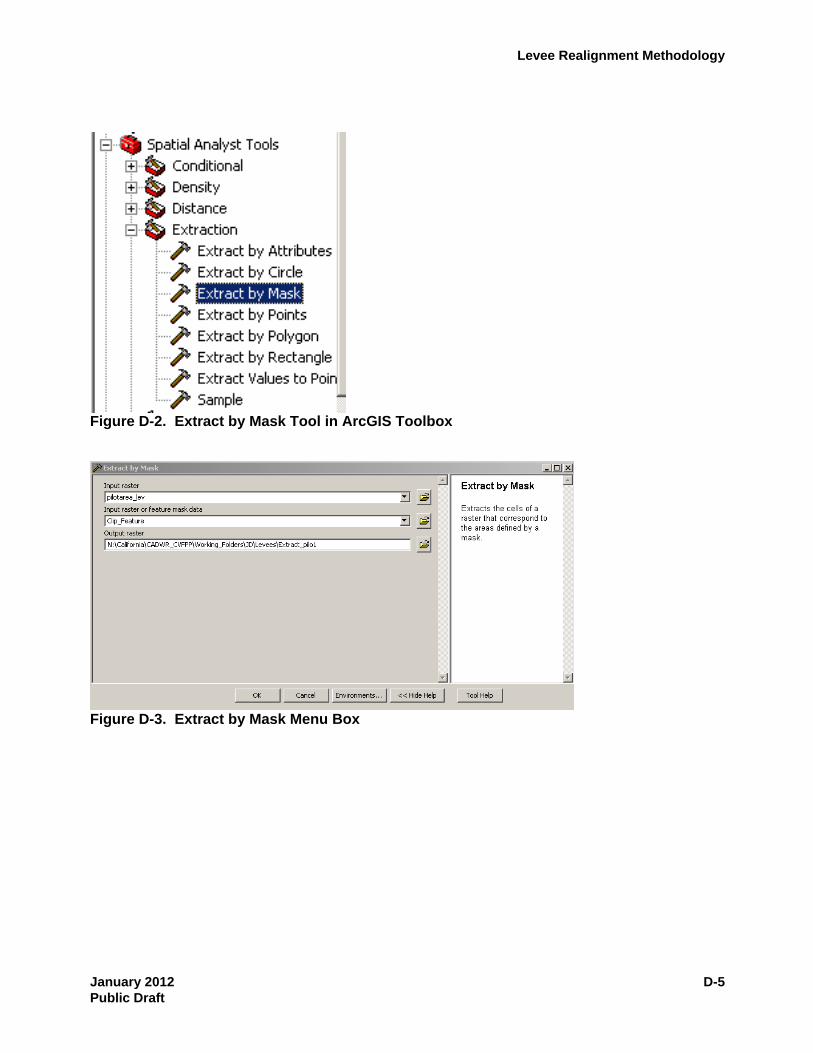
Levee Realignment Methodology
January 2012 D-5 Public Draft
Figure D-2. Extract by Mask Tool in ArcGIS Toolbox
Figure D-3. Extract by Mask Menu Box
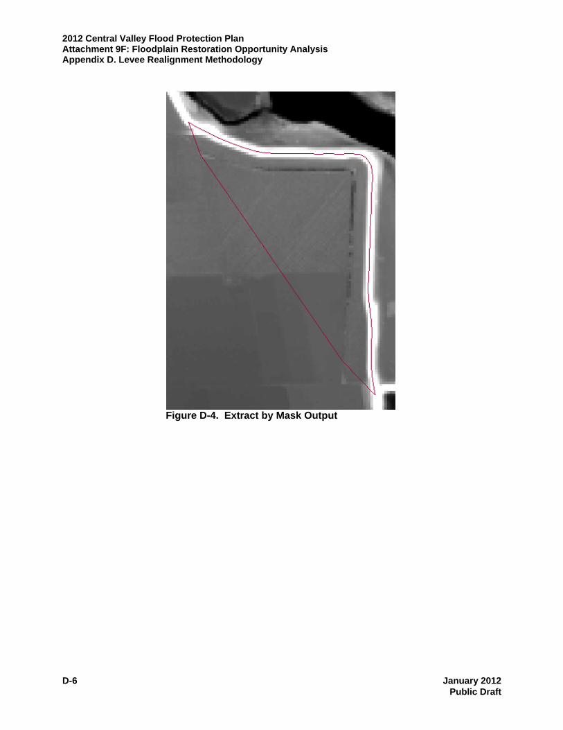
2012 Central Valley Flood Protection Plan Attachment 9F: Floodplain Restoration Opportunity Analysis Appendix D. Levee Realignment Methodology
D-6 January 2012 Public Draft
Figure D-4. Extract by Mask Output
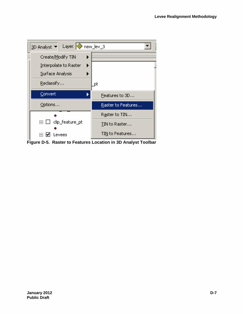
Levee Realignment Methodology
January 2012 D-7 Public Draft
Figure D-5. Raster to Features Location in 3D Analyst Toolbar
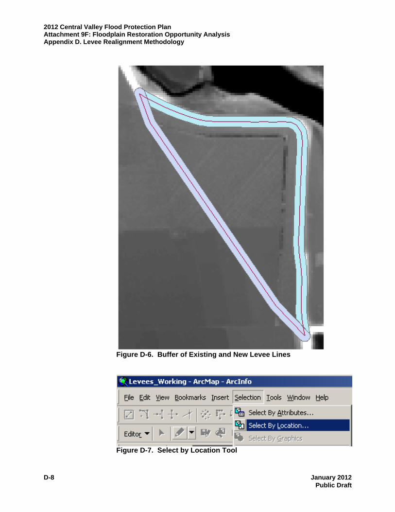
2012 Central Valley Flood Protection Plan Attachment 9F: Floodplain Restoration Opportunity Analysis Appendix D. Levee Realignment Methodology
D-8 January 2012 Public Draft
Figure D-6. Buffer of Existing and New Levee Lines
Figure D-7. Select by Location Tool
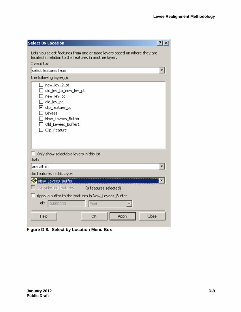
Levee Realignment Methodology
January 2012 D-9 Public Draft
Figure D-8. Select by Location Menu Box
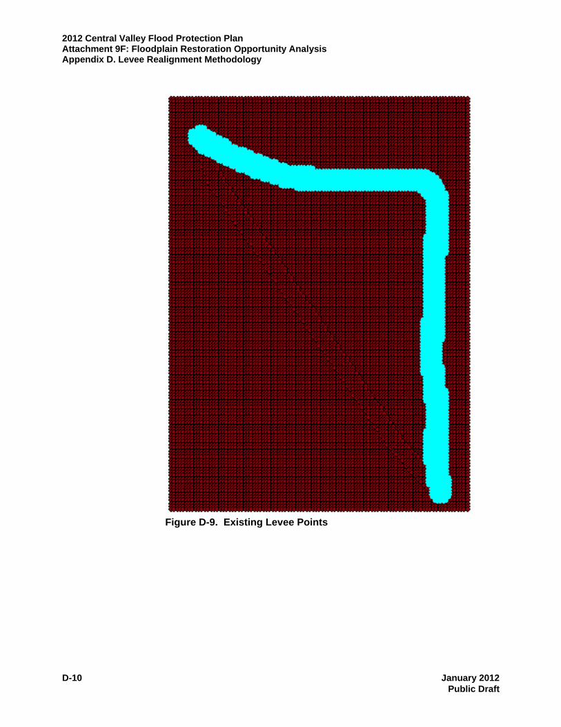
2012 Central Valley Flood Protection Plan Attachment 9F: Floodplain Restoration Opportunity Analysis Appendix D. Levee Realignment Methodology
D-10 January 2012 Public Draft
Figure D-9. Existing Levee Points
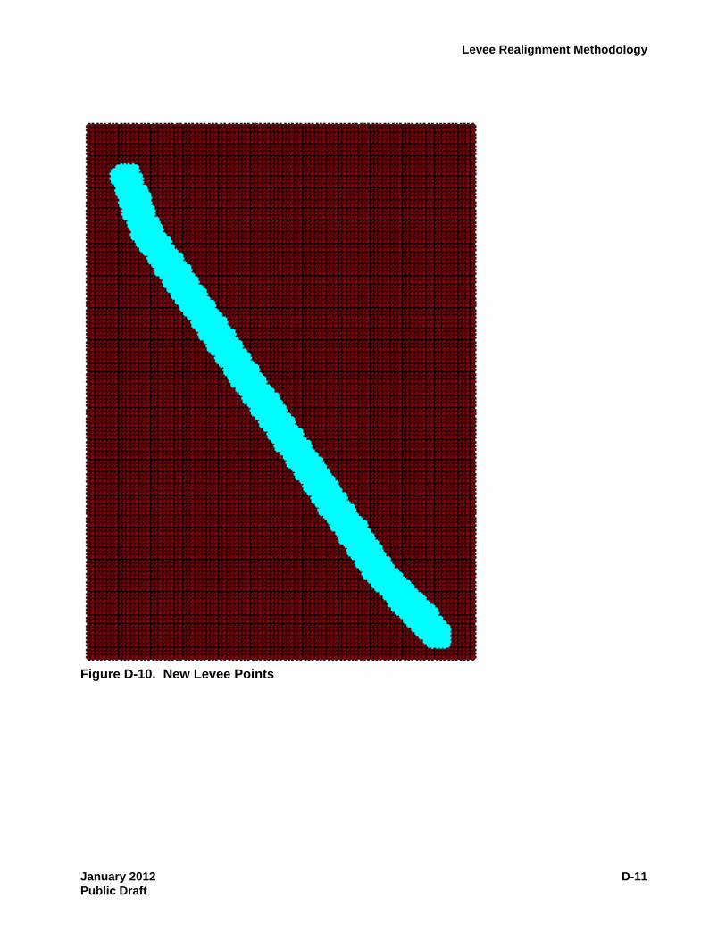
Levee Realignment Methodology
January 2012 D-11 Public Draft
Figure D-10. New Levee Points
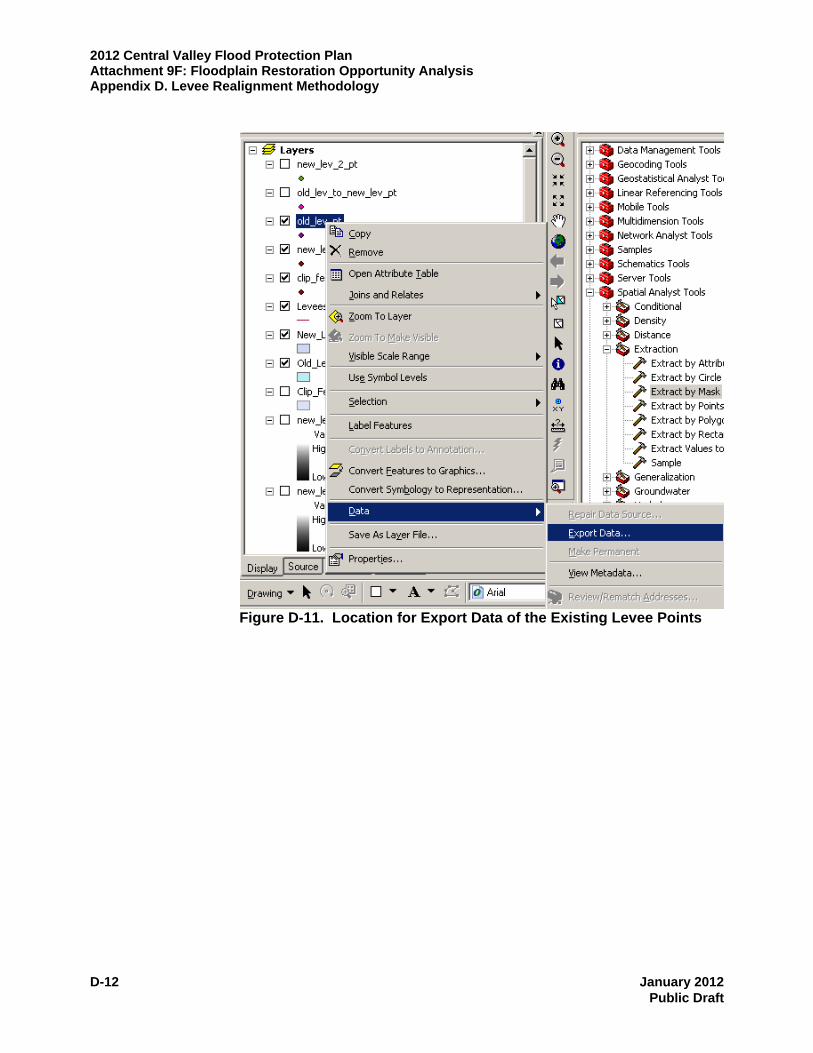
2012 Central Valley Flood Protection Plan Attachment 9F: Floodplain Restoration Opportunity Analysis Appendix D. Levee Realignment Methodology
D-12 January 2012 Public Draft
Figure D-11. Location for Export Data of the Existing Levee Points
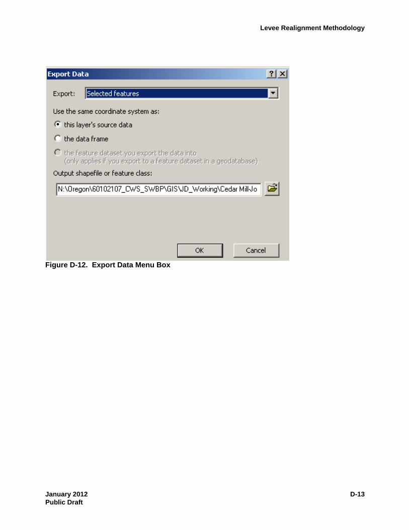
Levee Realignment Methodology
January 2012 D-13 Public Draft
Figure D-12. Export Data Menu Box
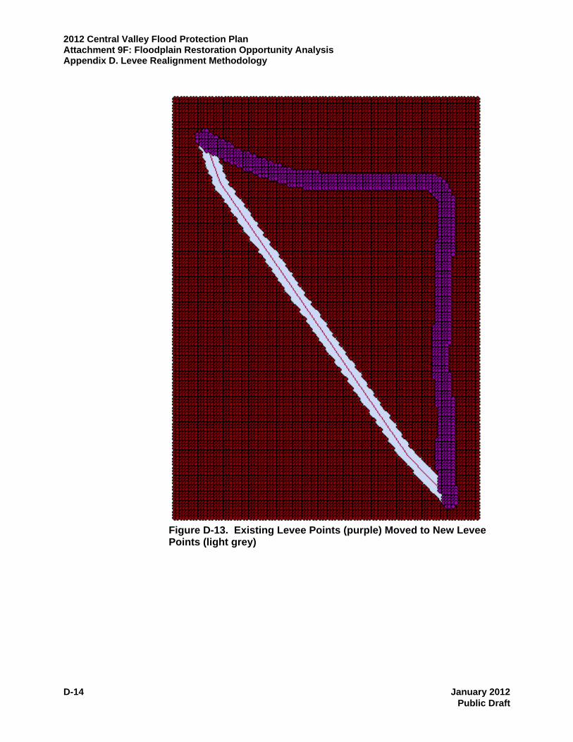
2012 Central Valley Flood Protection Plan Attachment 9F: Floodplain Restoration Opportunity Analysis Appendix D. Levee Realignment Methodology
D-14 January 2012 Public Draft
Figure D-13. Existing Levee Points (purple) Moved to New Levee Points (light grey)
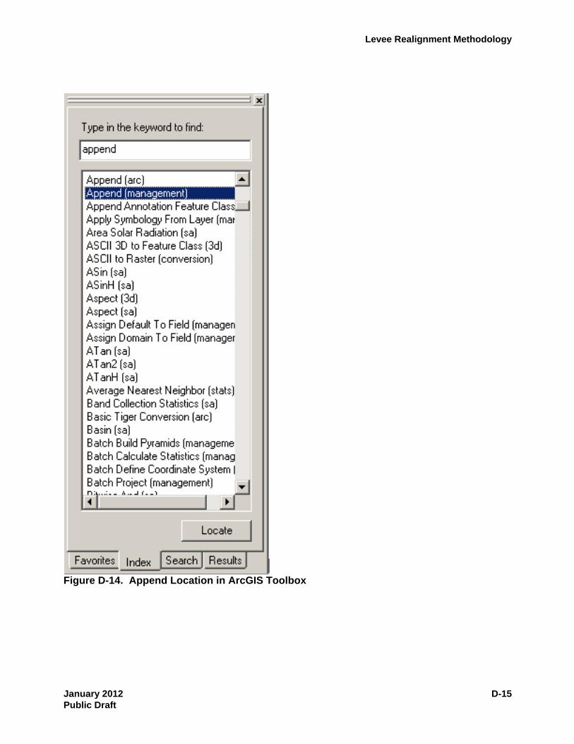
Levee Realignment Methodology
January 2012 D-15 Public Draft
Figure D-14. Append Location in ArcGIS Toolbox
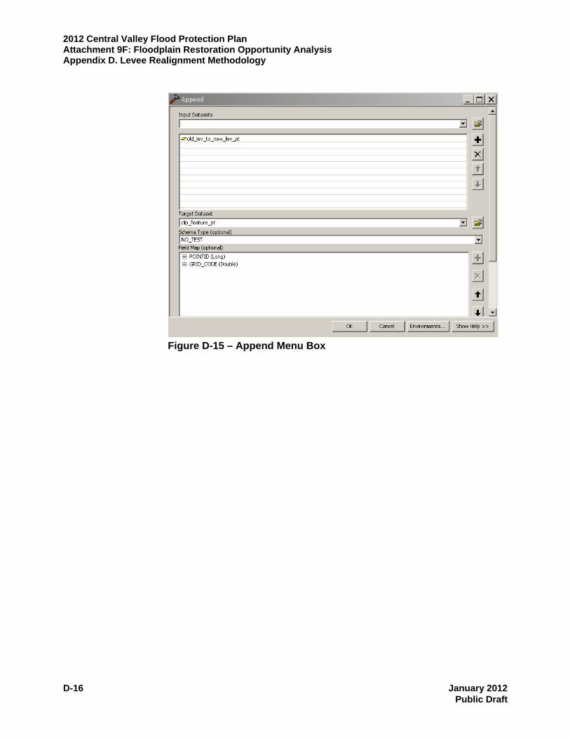
2012 Central Valley Flood Protection Plan Attachment 9F: Floodplain Restoration Opportunity Analysis Appendix D. Levee Realignment Methodology
D-16 January 2012 Public Draft
Figure D-15 – Append Menu Box
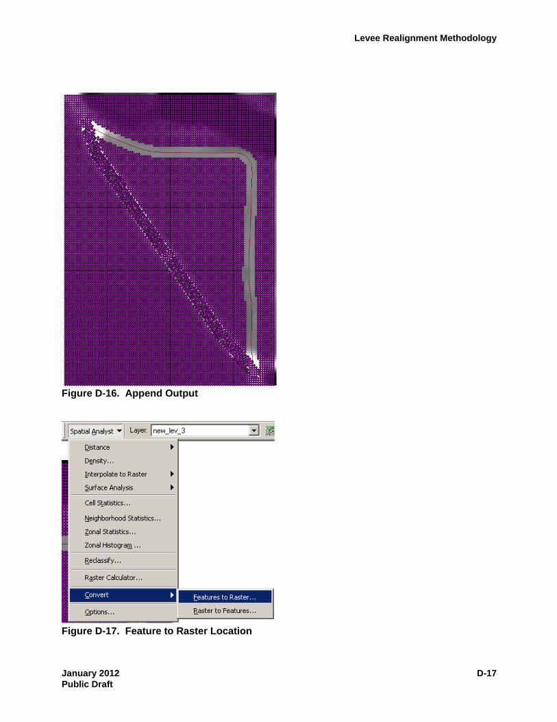
Levee Realignment Methodology
January 2012 D-17 Public Draft
Figure D-16. Append Output
Figure D-17. Feature to Raster Location
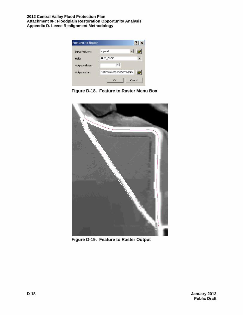
2012 Central Valley Flood Protection Plan Attachment 9F: Floodplain Restoration Opportunity Analysis Appendix D. Levee Realignment Methodology
D-18 January 2012 Public Draft
Figure D-18. Feature to Raster Menu Box
Figure D-19. Feature to Raster Output
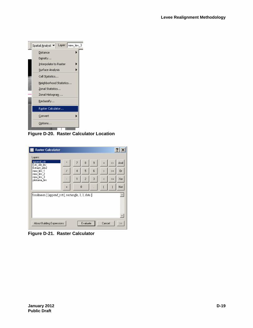
Levee Realignment Methodology
January 2012 D-19 Public Draft
Figure D-20. Raster Calculator Location
Figure D-21. Raster Calculator
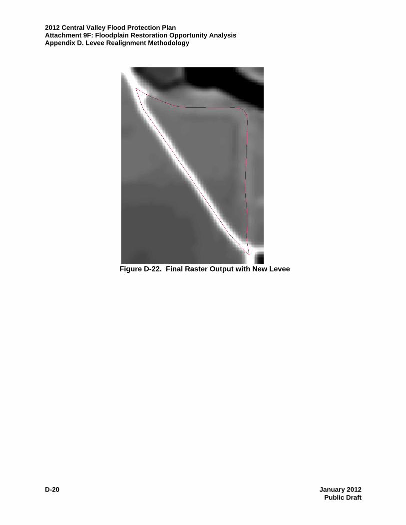
2012 Central Valley Flood Protection Plan Attachment 9F: Floodplain Restoration Opportunity Analysis Appendix D. Levee Realignment Methodology
D-20 January 2012 Public Draft
Figure D-22. Final Raster Output with New Levee
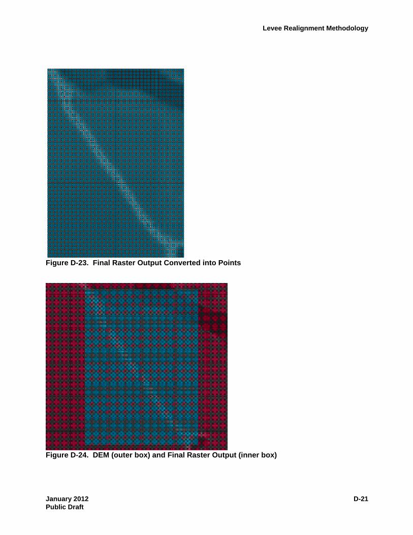
Levee Realignment Methodology
January 2012 D-21 Public Draft
Figure D-23. Final Raster Output Converted into Points
Figure D-24. DEM (outer box) and Final Raster Output (inner box)
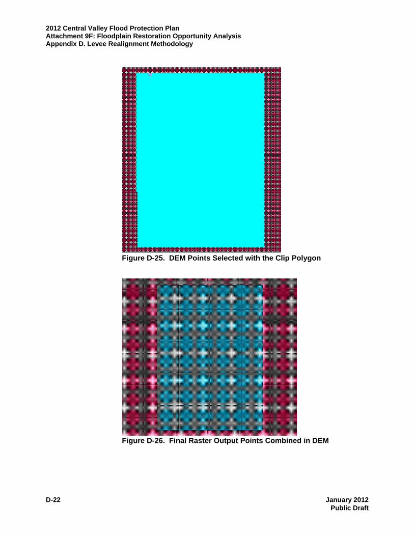
2012 Central Valley Flood Protection Plan Attachment 9F: Floodplain Restoration Opportunity Analysis Appendix D. Levee Realignment Methodology
D-22 January 2012 Public Draft
Figure D-25. DEM Points Selected with the Clip Polygon
Figure D-26. Final Raster Output Points Combined in DEM
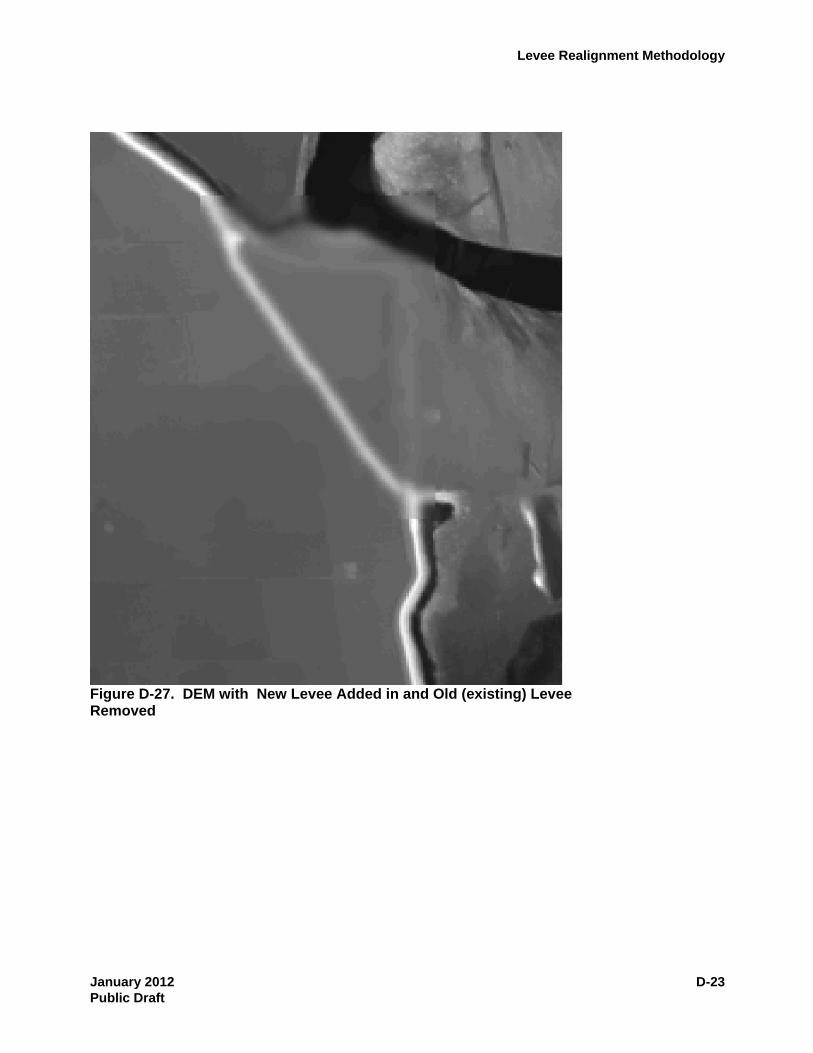
Levee Realignment Methodology
January 2012 D-23 Public Draft
Figure D-27. DEM with New Levee Added in and Old (existing) Levee Removed

2012 Central Valley Flood Protection Plan Attachment 9F: Floodplain Restoration Opportunity Analysis Appendix D. Levee Realignment Methodology
D-24 January 2012 Public Draft
This page left blank intentionally.
STATE OF CALIFORNIA THE NATURAL RESOURCES AGENCY DEPARTMENT OF WATER RESOURCES
Public Draft 2012 Central Valley Flood Protection Plan
Attachment 9F: Floodplain Restoration Opportunity Analysis – Appendix E. Synthetic vs. Observed Hydrographs
January 2012

January 2012 Public Draft
This page left blank intentionally.
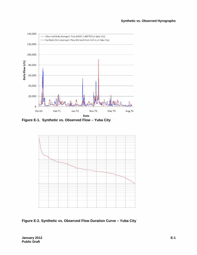
Synthetic vs. Observed Hyrographs
January 2012 E-1 Public Draft
Figure E-1. Synthetic vs. Observed Flow – Yuba City
Figure E-2. Synthetic vs. Observed Flow Duration Curve – Yuba City
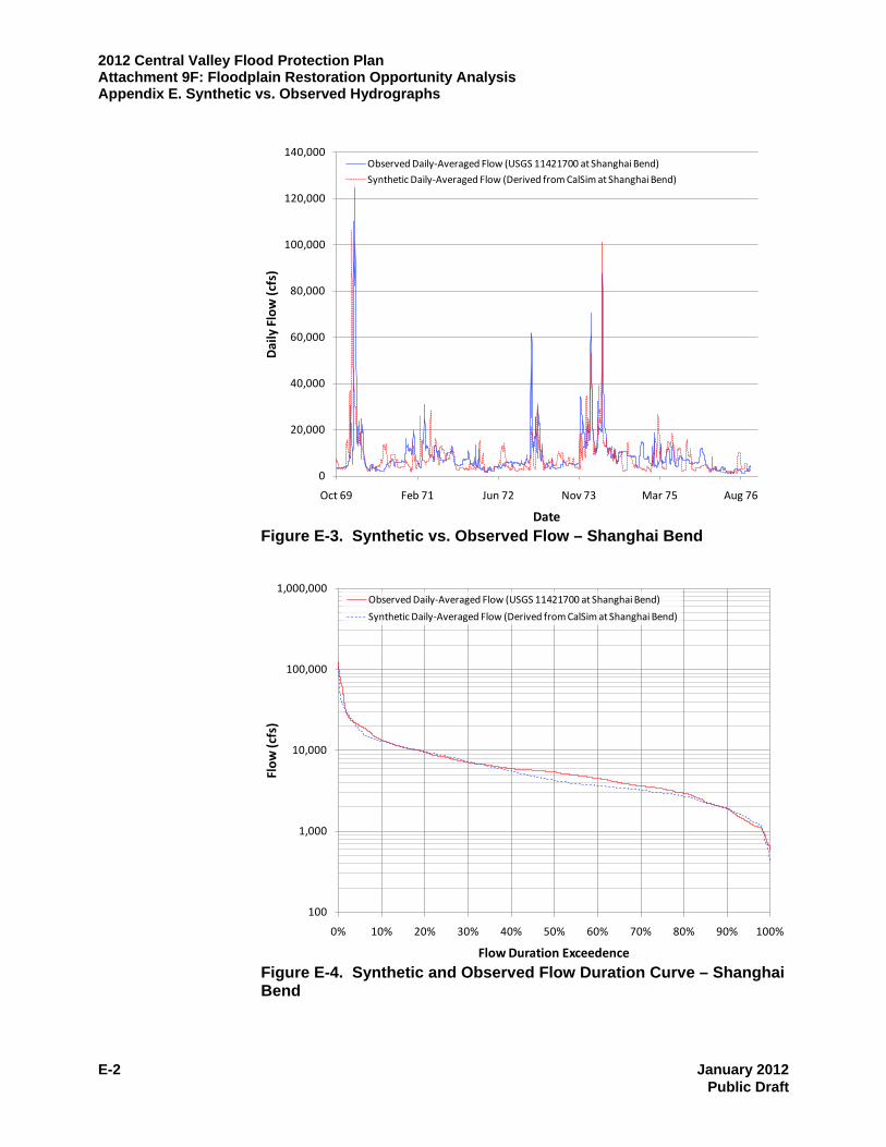
2012 Central Valley Flood Protection Plan Attachment 9F: Floodplain Restoration Opportunity Analysis Appendix E. Synthetic vs. Observed Hydrographs
E-2 January 2012 Public Draft
0
20,000
40,000
60,000
80,000
100,000
120,000
140,000
Oct 69 Feb 71 Jun 72 Nov 73 Mar 75 Aug 76
Daily
Flo
w (c
fs)
Date
Observed Daily-Averaged Flow (USGS 11421700 at Shanghai Bend)Synthetic Daily-Averaged Flow (Derived from CalSim at Shanghai Bend)
Figure E-3. Synthetic vs. Observed Flow – Shanghai Bend
100
1,000
10,000
100,000
1,000,000
0% 10% 20% 30% 40% 50% 60% 70% 80% 90% 100%
Flow
(cfs
)
Flow Duration Exceedence
Observed Daily-Averaged Flow (USGS 11421700 at Shanghai Bend)Synthetic Daily-Averaged Flow (Derived from CalSim at Shanghai Bend)
Figure E-4. Synthetic and Observed Flow Duration Curve – Shanghai Bend
STATE OF CALIFORNIA THE NATURAL RESOURCES AGENCY DEPARTMENT OF WATER RESOURCES
Public Draft 2012 Central Valley Flood Protection Plan
Attachment 9F: Floodplain Restoration Opportunity Analysis – Appendix F. HEC-EFM Ecosystem Functional Relationships January 2012

January 2012 Public Draft
This page left blank intentionally.
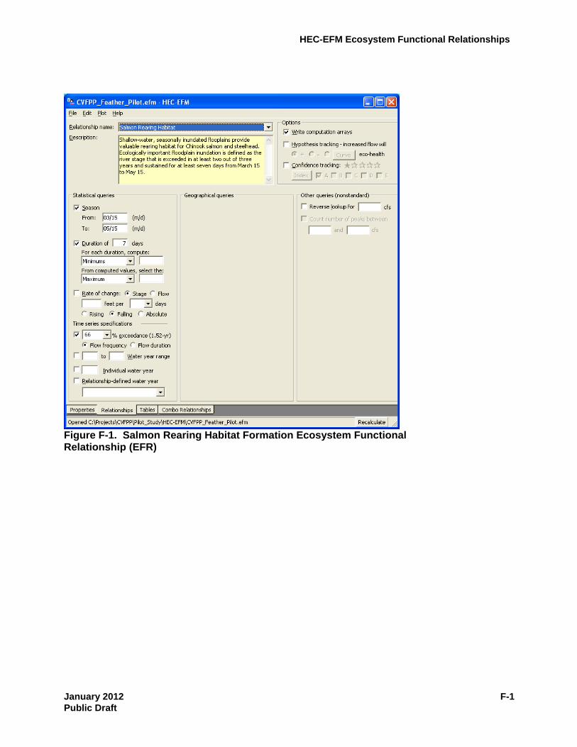
HEC-EFM Ecosystem Functional Relationships
January 2012 F-1 Public Draft
Figure F-1. Salmon Rearing Habitat Formation Ecosystem Functional Relationship (EFR)
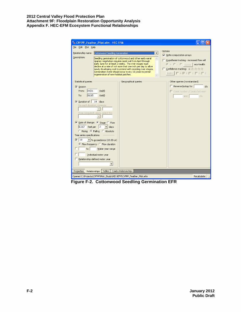
2012 Central Valley Flood Protection Plan Attachment 9F: Floodplain Restoration Opportunity Analysis Appendix F. HEC-EFM Ecosystem Functional Relationships
F-2 January 2012 Public Draft
Figure F-2. Cottonwood Seedling Germination EFR
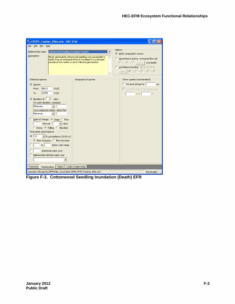
HEC-EFM Ecosystem Functional Relationships
January 2012 F-3 Public Draft
Figure F-3. Cottonwood Seedling Inundation (Death) EFR
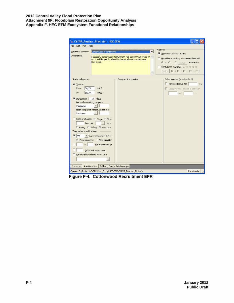
2012 Central Valley Flood Protection Plan Attachment 9F: Floodplain Restoration Opportunity Analysis Appendix F. HEC-EFM Ecosystem Functional Relationships
F-4 January 2012 Public Draft
Figure F-4. Cottonwood Recruitment EFR
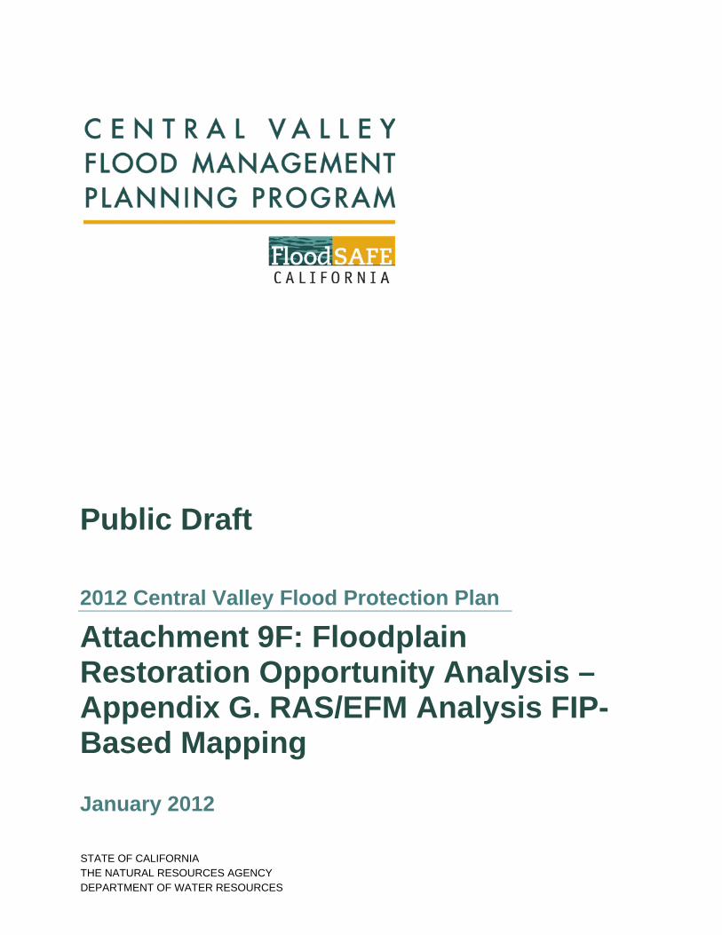
STATE OF CALIFORNIA THE NATURAL RESOURCES AGENCY DEPARTMENT OF WATER RESOURCES
Public Draft
2012 Central Valley Flood Protection Plan
Attachment 9F: Floodplain Restoration Opportunity Analysis – Appendix G. RAS/EFM Analysis FIP-Based Mapping January 2012

2 January 2012 Public Draft
This page left blank intentionally.
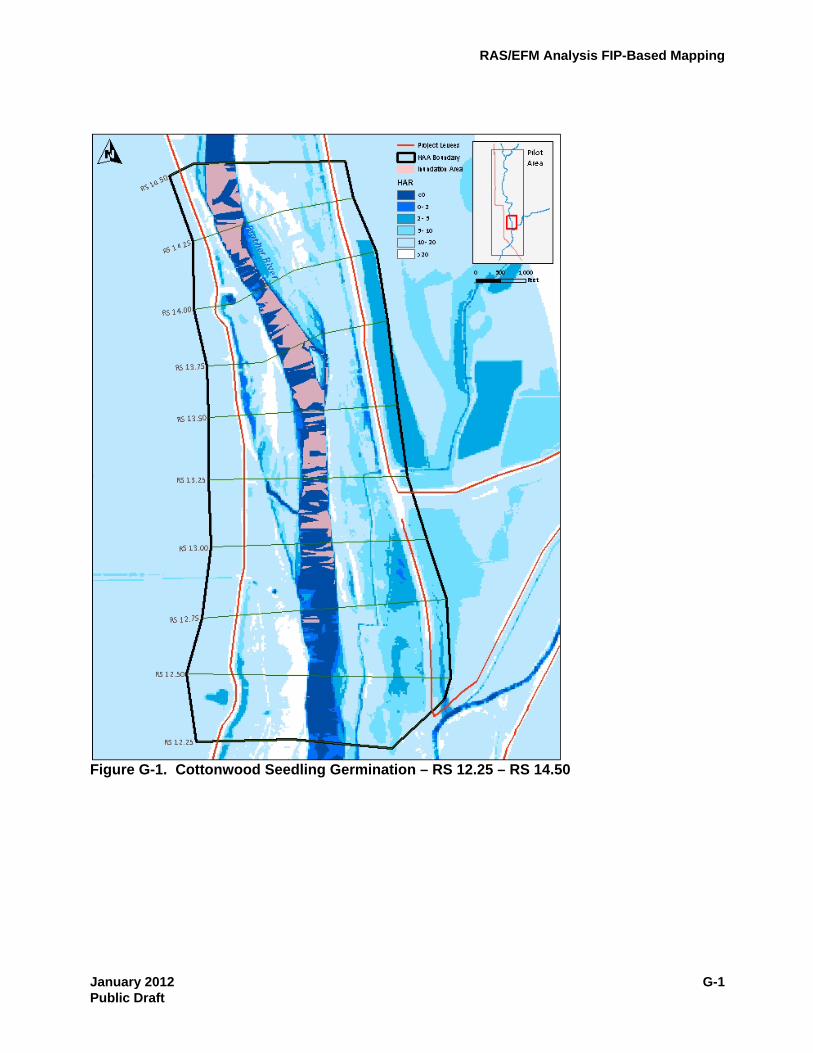
RAS/EFM Analysis FIP-Based Mapping
January 2012 G-1 Public Draft
Figure G-1. Cottonwood Seedling Germination – RS 12.25 – RS 14.50
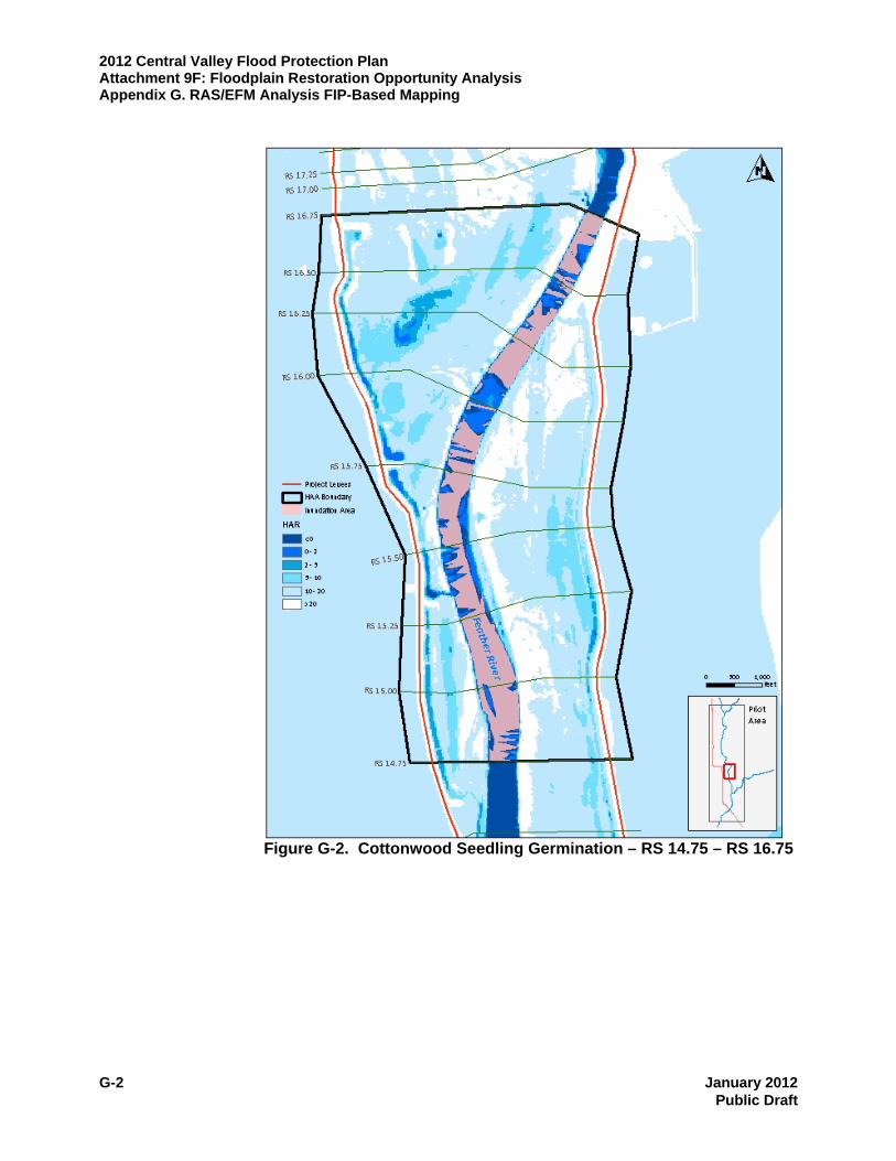
2012 Central Valley Flood Protection Plan Attachment 9F: Floodplain Restoration Opportunity Analysis Appendix G. RAS/EFM Analysis FIP-Based Mapping
G-2 January 2012 Public Draft
Figure G-2. Cottonwood Seedling Germination – RS 14.75 – RS 16.75
RAS/EFM Analysis FIP-Based Mapping
January 2012 G-3 Public Draft
Figure G-3. Cottonwood Seedling Germination – RS 17.00 – RS 21.00
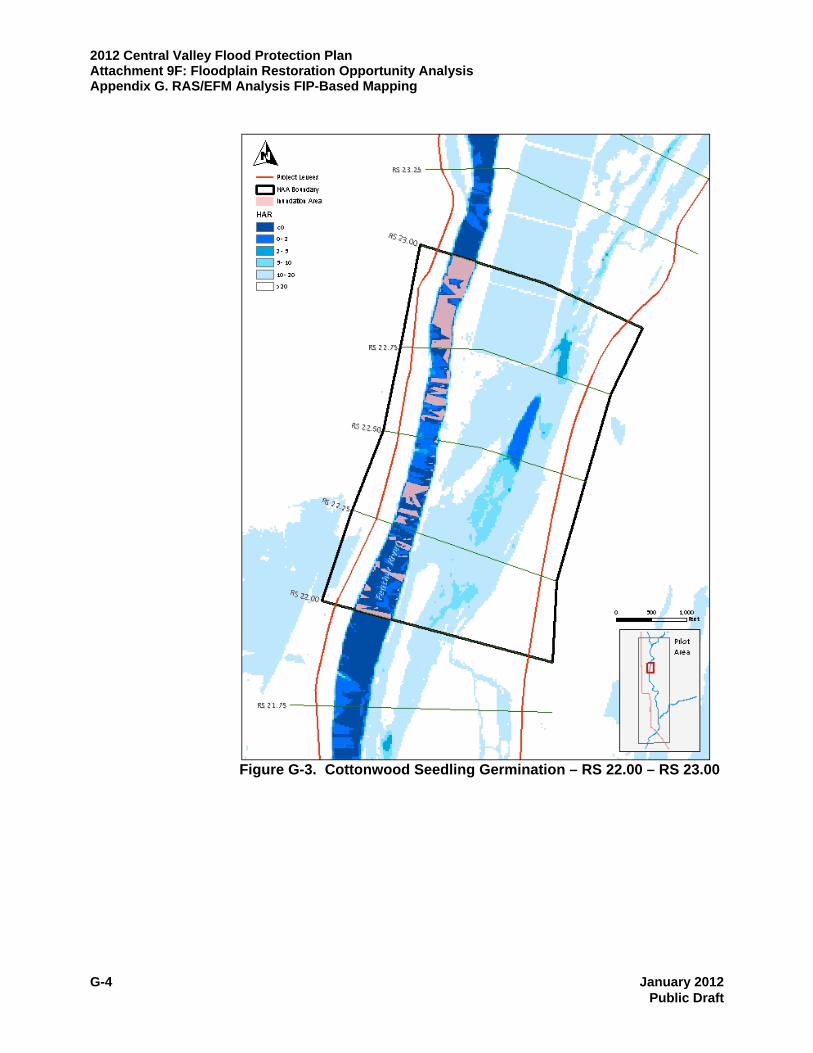
2012 Central Valley Flood Protection Plan Attachment 9F: Floodplain Restoration Opportunity Analysis Appendix G. RAS/EFM Analysis FIP-Based Mapping
G-4 January 2012 Public Draft
Figure G-3. Cottonwood Seedling Germination – RS 22.00 – RS 23.00
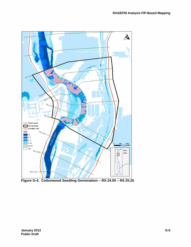
RAS/EFM Analysis FIP-Based Mapping
January 2012 G-5 Public Draft
Figure G-4. Cottonwood Seedling Germination – RS 24.00 – RS 25.25
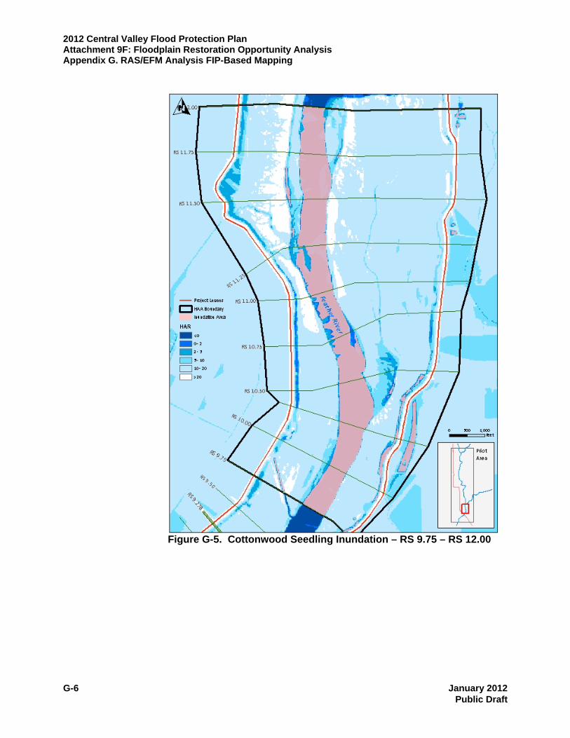
2012 Central Valley Flood Protection Plan Attachment 9F: Floodplain Restoration Opportunity Analysis Appendix G. RAS/EFM Analysis FIP-Based Mapping
G-6 January 2012 Public Draft
Figure G-5. Cottonwood Seedling Inundation – RS 9.75 – RS 12.00
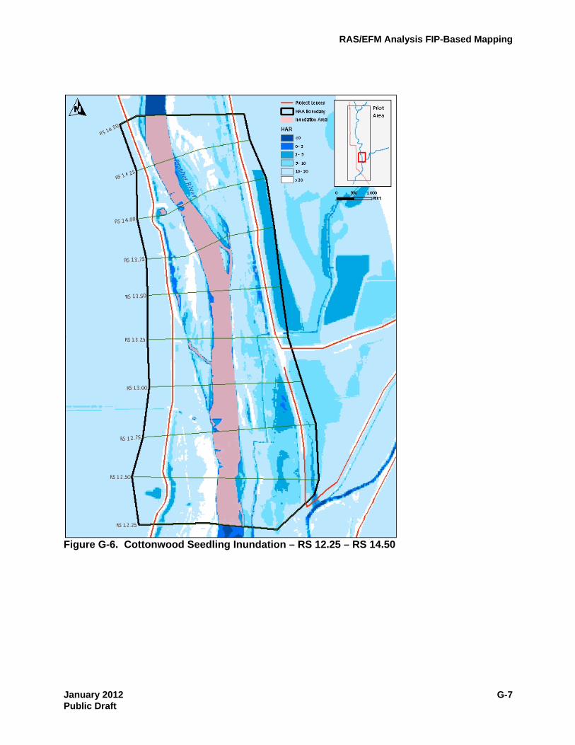
RAS/EFM Analysis FIP-Based Mapping
January 2012 G-7 Public Draft
Figure G-6. Cottonwood Seedling Inundation – RS 12.25 – RS 14.50
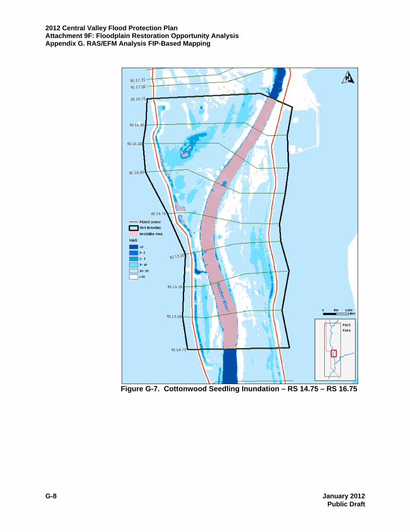
2012 Central Valley Flood Protection Plan Attachment 9F: Floodplain Restoration Opportunity Analysis Appendix G. RAS/EFM Analysis FIP-Based Mapping
G-8 January 2012 Public Draft
Figure G-7. Cottonwood Seedling Inundation – RS 14.75 – RS 16.75
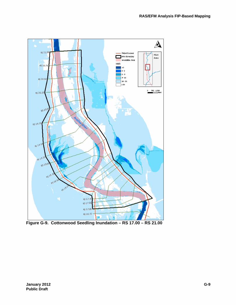
RAS/EFM Analysis FIP-Based Mapping
January 2012 G-9 Public Draft
Figure G-9. Cottonwood Seedling Inundation – RS 17.00 – RS 21.00
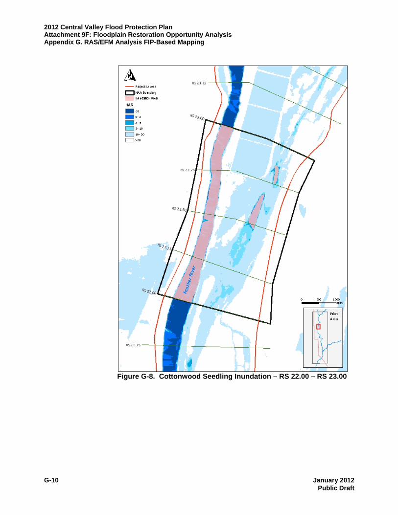
2012 Central Valley Flood Protection Plan Attachment 9F: Floodplain Restoration Opportunity Analysis Appendix G. RAS/EFM Analysis FIP-Based Mapping
G-10 January 2012 Public Draft
Figure G-8. Cottonwood Seedling Inundation – RS 22.00 – RS 23.00

RAS/EFM Analysis FIP-Based Mapping
January 2012 G-11 Public Draft
Figure G-11. Cottonwood Seedling Inundation – RS 24.00 – RS 25.25

2012 Central Valley Flood Protection Plan Attachment 9F: Floodplain Restoration Opportunity Analysis Appendix G. RAS/EFM Analysis FIP-Based Mapping
G-12 January 2012 Public Draft
This page left blank intentionally.


STATE OF CALIFORNIA THE NATURAL RESOURCES AGENCY
DEPARTMENT OF WATER RESOURCES


![River Restoration to Achieve a Stage 0 Conditionapproach to floodplain restoration often referred to as “Stage 0 [zero]” stream restoration. This term is commonly applied to actions](https://img.pdfslide.net/doc/110x75/611feaa807e6c379a344c880/river-restoration-to-achieve-a-stage-0-condition-approach-to-floodplain-restoration.jpg)