Embed Size (px)
Citation preview

The Bang for the Birr
Public Expenditures and Rural Welfare in Ethiopia
Tewodaj Mogues, Gezahegn Ayele, and Zelekawork Paulos
RESEARCHREPORT 160
IFPRI
INTERNATIONAL FOODPOLICY RESEARCH INSTITUTEsustainable solutions for ending hunger and poverty
®

Copyright © 2008 International Food Policy Research Institute. All rights reserved. Sections of this material may be reproduced for personal and not-for-profit use without the express written permission of but with acknowledgment to IFPRI. To reproduce material contained herein for profit or commercial use requires express written permission. To obtain permission, contact the Communications Division <[email protected]>.
International Food Policy Research Institute2033 K Street, NWWashington, D.C. 20006-1002, U.S.A.Telephone +1-202-862-5600www.ifpri.org
DOI: 10.2499/9780896291690RR160
Library of Congress Cataloging-in-Publication Data
Tewodaj Mogues. The bang for the birr : public expenditures and rural welfare in Ethiopia / Tewodaj Mogues, Gezahegn Ayele and Zelekawork Paulos. p. cm.—(IFPRI research report ; 160) Includes bibliographical references. ISBN 978-0-89629-169-0 (alk. paper) 1. Government spending policy—Ethiopia. 2. Rural poor—Ethiopia. 3. Social service, Rural—Ethiopia. I. Gezahegn Ayele. II. Zelekawork Paulos. III. International Food Policy Research Institute. IV. Title. V. Title: Public expenditures and rural welfare in Ethiopia. VI. Series: Research report (International Food Policy Research Institute) ; 160.HJ7928.T49 2008336.3′90963—dc22 2008042166
Contents
List of Tables iv
List of Figures vi
Foreword vii
Acknowledgments viii
Acronyms and Abbreviations ix
Summary x
1. Public Spending and Rural Welfare in Ethiopia 1
2. Empirical Approaches to Assessing the Impact of Public Spending 4
3. Development Strategy and Development Outcomes in Ethiopia 8
4. Strategies, Public Spending, and Performance in Key Sectors 14
5. Conceptual Framework of Public Spending, Public Services, and Private Assets 29
6. Empirical Strategy 33
7. Estimation 38
8. Conclusions and Policy Considerations 68
Appendix 70
References 80
iii

Tables
3.1 Per capita own-source and federal transfer components of regional budgets in Ethiopia, 1997 9
3.2 Geographic distribution of poverty: Headcount poverty rates across regions, 1995 and 1999 11
4.1 Public expenditures on selected sectors, 1984–2005 (percent of total public expenditure) 15
4.2 Composition of total expenditure by level of government, 1998 16
4.3 Capital and recurrent road infrastructure expenditures by region, 1998 20
4.4 Density of all-weather roads, selected years 20
4.5 Road density by road type, 2003 20
4.6 Total national expenditure on agriculture and natural resources, 1993–2000 (millions, constant 1995 birr) 22
4.7 Real per capita regional expenditure on agricultural and natural resources, 1993–2000 (birr) 22
4.8 Yield of annual crops by region, 1995–2000 (quintals per hectare) 23
4.9 Literacy rate, 1990 and 2002 (percent of 15-year-olds and above) 23
4.10 Primary school (grades 1–8) gross enrollment ratio, 1994–2003 24
4.11 Primary school (grades 1–8) pupil-to-teacher ratio, selected years 24
4.12 Immunization and child mortality rates for Ethiopia and selected African countries, 2002 25
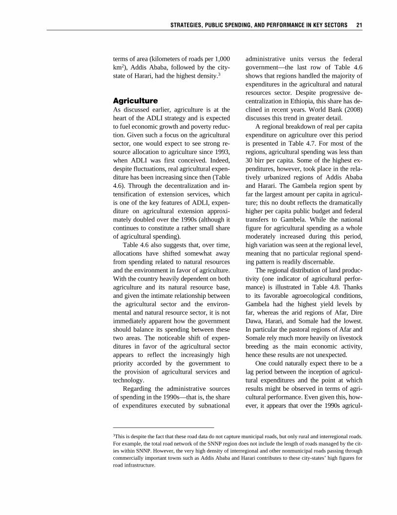
4.13 Potential health service coverage, selected years (percent) 27
4.14 Average distance to the nearest health center, 2000 (km) 27
4.15 Health expenditures in Ethiopia and other low-income country groups, 2001 28
7.1 Descriptive statistics for Ethiopia’s rural population 39
7.2 Indirect and direct countrywide rural welfare effects of public services and infrastructure access 40
7.3 Average countrywide rural welfare effects of public services and infrastructure access 41
iv

7.4 Direct and indirect region-specific effects of access to services in all four sectors 42
7.5 Robustness of short first-stage model to exclusion of observations 44
7.6 Regionally differentiated role of public services, including indirect effects 46
7.7 Regionally differentiated role of public services: Average effects 48
7.8 Robustness of primary first-stage model to exclusion of observations 50
7.9 Public spending and sectoral outcomes: Specification with cross-sector complementarities 53
7.10 Public spending and sectoral outcomes: Specification including agricultural inputs as a determinant of agricultural productivity 54
7.11 Public spending and sectoral outcomes: Specification including cross-sector complementarities and agricultural inputs 56
7.12 Public spending and sectoral outcomes: Base specification with neither sector complementarities nor agricultural inputs 58
7.13 Public spending and sectoral outcomes: Summary of public investment coefficients for different parametric assumptions 60
7.14 Impact of public expenditure on household welfare: Two alternative first-stage specifications 61
7.15 Impact of public expenditure on household welfare: Four alternative second-stage parameter value assumptions 64
7.16 Impact of public expenditure on household welfare: Robustness to exclusion of observations 66
A.1 Per capita household expenditure, based on the Household Income, Consumption and Expenditure (HICE) Surveys 71
A.2 Per-adult-equivalent household expenditure, based on the Welfare Monitoring Surveys 71
A.3 Spending in each region, 1998 (percent of total regional expenditures) 72
A.4 Zonal averages for selected variables used in second-stage regression 73
A.5 Second-stage results based on parameter assumptions d = 0.02, r = 0.02 75
A.6 Second-stage results based on parameter assumptions d = 0.10, r = 0.10 76
A.7 Second-stage results based on parameter assumptions d = 0.02, r = 0.10 77
A.8 Second-stage results based on parameter assumptions d = 0.10, r = 0.02 78
tables v
Figures
3.1 Per capita household expenditure by region 12
3.2 Real per-adult-equivalent household expenditure 13
4.1 Road density in Ethiopia and Sub-Saharan African countries 18
5.1 Framework for the effect of public expenditures on rural household welfare 30
A.1 Administrative map of Ethiopia 70
vi

Foreword
vii
T his report explores and compares the impacts of different types of public spending on rural household welfare in Ethiopia. The analysis of public financial and household-level data reveals that returns to road investments are significantly higher than returns
to other spending but are much more variable across regions. This regional variability suggests that the government should carefully consider regionally differentiated investment priorities. Some evidence indicates that the returns to road spending are increasing over time, with higher returns to road investments seen in areas with better-developed road networks. The household expenditure impacts of per capita public expenditure in agriculture are substantially smaller and do not emerge as statistically significant. A separate examination of the three stages of analysis shows that—while the contribution of a strong agricultural sector to the incomes of both farming and nonfarming rural households is strong—the link between public expenditures in agriculture and performance in agriculture is poor, resulting in nonsignificant returns to agricultural spending. This suggests that a more careful examination of the composition as well as the execution of the agricultural budget would be advisable, in order to explore how it can be made more effective. There is also some evidence that the most significant effects of agricultural expenditures on rural households are observed in the most ur-banized regions, pointing to the potentially important impact of market proximity on returns to public interventions in agriculture. Expenditures in the education sector have greater rural welfare returns than agriculture spending but on average lower returns than road spending. However, while returns to road spending seem to be concentrated in a few regions, those to education have a wider reach across many regions and the returns are less varied in magnitude across regions. Expenditures in the health sector do not have widely significant effects on rural incomes—suggesting, together with other findings in the empirical work, that nonincome measures of well-being should be considered in the analysis of future public expenditures.
Joachim von BraunDirector General, IFPRI

Acknowledgments
T his paper is the result of a research project that was part of the Ethiopian Strategy Sup-port Program (ESSP).
The authors gratefully acknowledge Shenggen Fan for his valuable comments on the various drafts. We also thank two anonymous referees for careful and detailed comments. A previous version of this paper was much improved by comments from an anonymous reviewer for the International Food Policy Research Institute (IFPRI) Discussion Paper series. This text has benefited from helpful discussions with several other researchers at IFPRI, as well as com-ments by participants in seminars at which the findings were presented, including a conference sponsored by the Centre for the Study of African Economies in Oxford, the annual meetings of the American Agricultural Economics Association, a joint ESSP/Addis Ababa University symposium, and the annual meetings of the Midwest Economics Association. Thanks are also due to various Ethiopian government ministries and institutions for mak-ing secondary data available, especially the Ministry of Finance and Economic Development (MOFED), the Central Statistical Authority, the Ministry of Health, and the Ethiopian Roads Authority. Any remaining errors are our own.
viii

Acronyms and Abbreviations
ADLI Agricultural Development–Led Industrialization
CSA Central Statistical Authority
ESSP Ethiopian Strategy Support Program
GDP gross domestic product
HICE Household Income, Consumption and Expenditure (Survey)
IFPRI International Food Policy Research Institute
kWh kilowatts per hour
MOFED Ministry of Finance and Economic Development
OLS ordinary least squares
PTR pupil-to-teacher ratio
RSDP Road Sector Development Program
SNNP Southern Nations, Nationalities, and Peoples
S-2SLS system-two-stage-least-squares
S-3SLS system-three-stage-least-squares
TVET technical and vocational education and training
ix

Summary
Over the past decade and a half, Ethiopia’s approach to promoting development and improving the lives of the country’s rural population has been driven by a govern-ment strategy called Agricultural Development–Led Industrialization (ADLI). This
strategy’s main goal is fast, broad-based development within the agricultural sector that can power economic growth. While ADLI stipulates regulatory, trade, market, and other poli-cies as engines of agricultural growth, it relies heavily on increasing public expenditure in agriculture and infrastructure, as well as in social sectors that are perceived as contributing to agricultural productivity. Thus Ethiopia’s public expenditure policy is at the heart of the policy measures intended to translate ADLI into reality. Given budget constraints, a critical and actionable research question is what kind of relative contributions different types of public investments make to welfare. Any answer to this question will have important implications for expenditure policy, especially the portfolio composition of public resources. This research report explores and compares the impacts of different types of public spend-ing on rural household welfare in Ethiopia. After an introduction to the topic in Chapter 1, Chapter 2 reviews the empirical and theoretical literature. Most of the studies examining the link between public expenditure and development outcomes fall into one of two categories. Studies in the first category explore how the size of overall public expenditure or public investment affects growth or poverty. The second category consists of studies that correlate spending in one economic sector with outcomes in that sector or with broader measures of welfare. Both categories of study can provide useful input into policymaking decisions. However, there is a striking lack of research aimed at examining how the composition of public spending affects key development outcomes—a particularly policy-relevant question. In the literature that does look comparatively at public spending across sectors, the empirical methods used include marginal benefit incidence analysis, general equilibrium models, and econometric approaches, which are all discussed in Chapter 2. Chapters 3 and 4 provide a foundation for the conceptual and empirical portion of the re-port by discussing Ethiopia’s development strategy, key trends in development outcomes, and patterns in public expenditures. In 2002 the Ethiopian government spelled out a development strategy whose main tenets were the continuation of ADLI and expanding fiscal and admin-istrative decentralization. The government’s public expenditure priorities have been strongly shaped by these two features of the development strategy. Chapter 5 describes the framework underlying the empirical analysis of the welfare re- turns to different types of public spending. It illustrates three stages of the analysis. The first highlights the role of access to public services in determining the welfare of rural house-holds, incorporating the way in which public services and sector-specific outcomes, such as school enrollment and road density, may contribute both directly and indirectly to that welfare. The second stage shows how public services and infrastructure are in turn determined by the amount of public financial resources committed to different sectors. The final stage of the
x
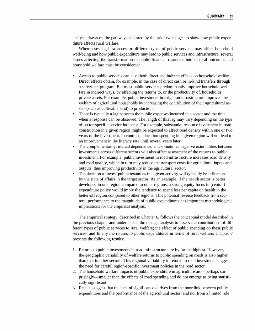
analysis draws on the pathways captured by the prior two stages to show how public expen-diture affects rural welfare. When assessing how access to different types of public services may affect household well-being and how public expenditure may lead to public services and infrastructure, several issues affecting the transformation of public financial resources into sectoral outcomes and household welfare must be considered:
• Accesstopublicservicescanhavebothdirectandindirecteffectsonhouseholdwelfare.Direct effects obtain, for example, in the case of direct cash or in-kind transfers through a safety-net program. But most public services predominantly improve household wel-fare in indirect ways, by affecting the returns to, or the productivity of, households’ private assets. For example, public investment in irrigation infrastructure improves the welfare of agricultural households by increasing the contribution of their agricultural as-sets (such as cultivable land) to production.
• Thereistypicallyalagbetweenthepublicexpensesincurredinasectorandthetimewhen a response can be observed. The length of this lag may vary depending on the type of sector-specific service indicator. For example, substantial resource investment in road construction in a given region might be expected to affect road density within one or two years of the investment. In contrast, education spending in a given region will not lead to an improvement in the literacy rate until several years later.
• Thecomplementarity,mutualdependence,andsometimesnegativeexternalitiesbetweeninvestments across different sectors will also affect assessment of the returns to public investment. For example, public investment in road infrastructure increases road density and road quality, which in turn may reduce the transport costs for agricultural inputs and outputs, thus improving productivity in the agricultural sector.
• Thedecisiontoinvestpublicresourcesinagivenactivitywilltypicallybeinfluencedby the state of affairs in the target sector. As an example, if the health sector is better developed in one region compared to other regions, a strong equity focus in (central) expenditure policy would imply the tendency to spend less per capita on health in the better-off region compared to other regions. This potential reverse feedback from sec-toral performance to the magnitude of public expenditures has important methodological implications for the empirical analysis.
The empirical strategy, described in Chapter 6, follows the conceptual model described in the previous chapter and undertakes a three-stage analysis to assess the contributions of dif-ferent types of public services to rural welfare; the effect of public spending on these public services; and finally the returns to public expenditures in terms of rural welfare. Chapter 7 presents the following results:
1. Returns to public investments in road infrastructure are by far the highest. However, the geographic variability of welfare returns to public spending on roads is also higher than that in other sectors. This regional variability in returns to road investment suggests the need for careful region-specific investment policies in the road sector.
2. The household welfare impacts of public expenditure in agriculture are—perhaps sur-prisingly—smaller than the effects of road spending and do not emerge as being statisti-cally significant.
3. Results suggest that the lack of significance derives from the poor link between public expenditures and the performance of the agricultural sector, and not from a limited role
summary xi

of agriculture in promoting rural welfare. In fact the performance of the agricultural sector contributes significantly to rural consumption both when considering this role on average in Ethiopia and when assessing regionally disaggregated effects.
4. In contrast to the road infrastructure sector, returns to expenditures in education are characterized by wider reach, more homogeneity, and less intensity. Education spend-ing has widespread effects on welfare that are positive, significant, and similar across a broad range of regions (in contrast to returns to expenditures in the road sector, which are strongly concentrated in a few regions). The magnitude of these returns is more con-strained than in the road sector, but still larger and more significant than those to invest-ments in agriculture.
5. Rural welfare returns to spending in the health sector do not emerge strongly, with sig-nificant returns in only one region and a relatively low magnitude of birr-for-birr returns. This, together with other findings in the empirical work, suggests that nonincome mea-sures of well-being should be considered in the analysis of future public expenditures.
In conclusion, Chapter 8 points to an issue that goes beyond the scope of this report but is clearly worthy of additional study: the efficiency of public spending. The utility of public investments for household welfare and poverty reduction depends on at least two things: (1) the portfolio of the public budget and the appropriateness of the allocation of resources across sectors, and (2) the efficiency with which resources are used in any given sector or subsector. This report focuses on the former issue, provoking an inquiry into the second question. Such an inquiry is particularly important with regard to Ethiopian agricultural investments, both because agriculture strongly dominates Ethiopia’s economy and because the government’s development strategy emphasizes the agricultural sector. A substantial body of research sug-gests that a strategic focus on agriculture may be appropriate, given Ethiopia’s stage of devel-opment. Therefore an investigation into the drivers of efficiency in the country’s agricultural public spending may be the next important step in policy research in Ethiopia.
xii summary

C H A P T E R 1
Public Spending and Rural Welfare in Ethiopia
Over the past decade and a half, Ethiopia’s approach to bringing about development and to improving the lives of the country’s rural population has been driven by a govern-mental development strategy called Agricultural Development–Led Industrialization
(ADLI).1 The main goal of this strategy is to attain fast and broad-based development within the agricultural sector and to use this development to power economic growth. While ADLI stipulates regulatory, trade, market, and other policies as an engine of agricultural growth, it has also relied heavily on increasing public expenditure in agricultural and other infrastructure and social sectors that are perceived as contributing to agricultural productivity. Thus Ethiopia’s public expenditure policy is at the heart of the policy measures intended to translate ADLI into reality. Several prior studies have sought to evaluate the success or failure of ADLI by examining other governmental policies considered central to agricultural and rural development, such as the land tenure policy (for example Deininger and Jin 2006), reforms in agricultural input markets (for example Jayne et al. 2002) and agricultural output markets (for example Dercon 1995), policies regarding the agricultural extension system (for example Belay and Abebaw 2004; Benin, Ehui, and Pender 2004; Alene and Hassan 2005), food security programs (for example Farrington and Slater 2006; Gelan 2006), and rural en-ergy policy (for example Teferra 2002; Wolde-Ghiorgis 2002).2 However, few if any studies have explored whether the government’s public budget allocations have been consistent with the stipulated development strategy or with good practices for achieving development. Even less is known regarding the extent to which the actual public investments have achieved im-provements in household incomes. Given the budget constraints faced by governments, the critical and actionable research question with regard to public expenditures is often not whether certain types of public invest- ments contribute to welfare improvements, but rather how different types of public investments compare in terms of their relative contributions to welfare. Any answer to this question will have important implications for expenditure policy, especially in terms of the portfolio com-position of public resources.
1This strategy is not to be confused with Irma Adelman’s concept of ADLI, which stands for agricultural demand–led industrialization (Adelman 1984), although the Ethiopian government’s development strategy has several features that appear to draw from Adelman’s concept.
2These are but a few examples from this extensive body of literature, the bulk of which falls outside the scope of the present report.
1

This research report explores and com-pares the impacts of different types of public spending on rural household welfare in Ethiopia. As with the literature on public investment in other developing countries, discussed later, the few published papers on public expenditure in Ethiopia either have been based on general equilibrium models that simulate the effects of changes in over-all public spending (Agenor, Bayraktar, and El Aynaoui 2004) or have concentrated on examining how public spending in one particular sector affects performance in that sector (Collier, Dercon, and Mackin-non 2002). We are not aware of any other study comparing the welfare or poverty effects of different types of public expendi-ture in Ethiopia. For the purposes of this report, we use the terms public investment and public expenditure interchangeably. This distinc-tion, while critical in other contexts, is not useful in the present work because we are interested in more than just the physi-cal outcomes of public investment. When considering the number of school buildings, for example, one might examine only the role of capital expenditure (which is often referred to as “public investment” in other contexts) in education as it relates to the number of schools in a given region, with-out including recurrent expenditures for teacher salaries, supplies, and the like. How- ever, when one is interested in a broader measure of performance in the education sector (for example, the primary enrollment ratio), then both recurrent and capital expen-ditures in education must be seen as forms of investment in human capital. There- fore, unless otherwise noted, we herein refer to the total (recurrent and capital) amount of public expenditure interchangeably as pub-lic expenditure or public investment. The analysis in this report finds that, among the sectors considered, returns to public investments in road infrastructure are by far the highest. However, the geographic variability of welfare returns to public spending on roads is also higher than that
in other sectors. This regional variability in returns to road investment suggests the need for careful region-specific investment poli-cies in the road sector. Perhaps surprisingly, the household welfare impacts of public ex-penditure in agriculture are smaller than the effects of road spending, and in fact they do not emerge as being statistically significant. Results suggest that the lack of significance derives from the poor link between public expenditures and the performance of the ag-ricultural sector, and not from a limited role of agriculture in promoting rural welfare. Rather the performance of the agricultural sector contributes significantly to rural con-sumption both when considering this role on average in Ethiopia and when assessing regionally disaggregated effects. In contrast to the road infrastructure sector, returns to expenditures in educa-tion are characterized by wider reach, more homogeneity, and less intensity. Education spending has widespread effects on welfare in that these returns are positive, significant, and similar across a broad range of regions, in contrast to returns to expenditures in the road sector, which are strongly concen-trated in a few regions. The magnitude of these returns is more constrained than in the road sector, but still larger and more significant than those to investments in ag-riculture. Rural welfare returns to spending in the health sector do not emerge strongly, with significant returns in only one region and a relatively low magnitude of birr-for-birr returns. The following chapter first discusses the empirical literature on public invest-ment and development goals in developing countries; this is followed by a discussion of the existing evidence on public investment impacts in Ethiopia. To place the empirical strategy and estimation of public expendi-ture effects into context, Chapter 3 begins with a brief overview of the key currents of Ethiopia’s development strategy and the development outcomes seen over the past 15 years. This is juxtaposed in Chapter 4 against broad trends in public expenditure,
2 CHAPTER 1

with further detail provided for selected sec-tors, development strategies, expenditure trends, and performance. Chapter 5 presents the conceptual context for this report and explores some of the challenges inherent in such public expenditure analysis. Chapter
6 describes the econometric strategy based on the conceptual framework of the preced-ing section. A description of the data and the results of this estimation approach are given in Chapter 7, with overall conclusions presented in the last chapter.
PubliC sPEnding And RuRAl wElfARE in ETHioPiA 3

C H A P T E R 2
Empirical Approaches to Assessing the Impact of Public Spending
Most of the studies examining the link between public expenditure and development outcomes fall into one of two categories. Studies in the first category explore how the size of overall public expenditure or public investment affects growth or pov-
erty. Examples include Agenor, Bayraktar, and El Aynaoui (2004) (described in more detail subsequently), who examined the impact of shifting resources from recurrent to capital expen-diture in Ethiopia, and Aschauer (2000), who compared the contributions of overall stocks of public and private capital to the national income while accounting for the size, financing, and efficiency of public capital. The second category includes studies in which the authors sought to correlate spending in one economic sector with outcomes in that sector, or with broader welfare measures (for ex-ample Collier, Dercon, and Mackinnon [2002] on the health sector in Ethiopia, and Roseboom [2002] on agricultural research). Also included in this category are studies seeking to assess the effectiveness of aid by determining the extent to which aid contributes to growth and poverty reduction by supporting increases in certain types of public investment (for example Gomanee, Girma, and Morrissey [2003] on social sector investment). Both types of studies can provide useful input into policymaking decisions. However, there is a striking lack of research aimed at examining how the composition of public spending affects key development outcomes—a particularly policy-relevant question. Usually the main public investment decision facing policymakers is how to allocate an existing pool of public resources across various sectors, rather than whether to increase or decrease the public budget. The question of allocation is typically considered annually or as part of deliberations over a country’s medium-term strategy. Budget allocation is inherently a political process in developing and industrialized countries alike, and budget decisions will typically reflect a range of considerations in addition to overall economic growth or pov-erty reduction. There is considerable need for studies on which types of public investments contribute the most to development goals, as this information may help shape aspects of the budgeting process. Paternostro, Rajaram, and Tiongson (2007) noted that the relative lack of research-based studies comparing the effectiveness of different types of public expenditure in contributing to poverty reduction has prompted international donors and the governments of developing countries to equate pro-poor spending with social sector investments, leading to corresponding expenditure policies. However, a number of studies (to be discussed later) have suggested that in many developing countries the greatest contributions to poverty reduction are not necessar-ily derived from social sector spending, but rather from investments in “hard” infrastructure
4

such as roads, electrification, and agricul-tural research systems. In the absence of empirical evidence supporting development returns to public spending, considerations other than economic development may fill the vacuum created by this knowledge gap. Hence research on the relative returns to different types of public investment may contribute a great deal to improving policy decisions. Several methods have been employed to examine the contributions to development outcomes of public spending in different sectors. Marginal benefit incidence analysis has been commonly used to assess the rela-tive poverty orientation of various forms of investment. Ajwad and Wodon (2007) ex-amined municipalities with different income levels in Bolivia and compared the benefit incidence of education, water, sewerage, electricity, and telephone services. How-ever, this and several other studies employ-ing marginal benefit incidence analysis fail to incorporate the actual expenditure out-lays for these public services. Other studies have used general equi-librium models to project public invest-ment effects into the future; these include those by Dabla-Norris and Matovu (2002) on Ghana, Jung and Thorbecke (2003) on Tanzania and Zambia, and Lofgren and Robinson (2005) on several African coun-tries. Several of these studies focused on the effects of education, although other types of investment were analyzed as well. Devara-jan, Swaroop, and Zou (1996) used regres-sion analysis (ordinary least squares [OLS] and fixed effects models) to compare the growth effects of public expenditures across functional and economic classifications. Using various econometric methods, a series of papers have taken an altogether different approach to assessing the relative contribution of different types of spend-ing to agricultural income. Rather than by sector, this literature classifies expenditure by the extent to which they provide public goods or privately incurred subsidies. Using as the central explanatory variable the share
of public spending on private subsidies to total public expenditures, in cross-country panel regression in Latin America (All-cott, Lederman, and López 2006; López and Galinato 2007) and in both developed and developing countries (López and Islam 2008), these studies consistently find that reducing the share of private subsidies in expenditure would increase agricultural gross domestic product (GDP), reduce pov-erty, and make agricultural production more environmentally sustainable. Another set of studies, also relying on econometric panel data but focusing their analysis at the country level, employ simul-taneous equation–based models to study the effect of a range of sectoral expenditures on agricultural growth and poverty outcomes (for example Fan, Hazell, and Thorat 2000; Fan, Zhang, and Zhang 2002). These stud-ies used aggregate province-level data on public expenditure, public capital, sectoral performance indicators, labor and wage variables, and agricultural productivity and poverty. The models incorporated the vari-ous pathways by which spending may af-fect poverty, and they generally showed that public spending on agricultural, health, education, and other sectors built up public capital and improved public services at the sector level. Furthermore they showed that improved public services and sector-level development increased the incomes of rural residents both by fostering agricultural pro-ductivity, which improved agricultural in-comes, and by providing more nonfarm income opportunities, which increased both wages and off-farm employment. Improved agricultural productivity was also found to have a price effect, as it reduced agricultural prices relative to other prices. Both the price and the (farm and off-farm) income effects were found to contribute positively to pov-erty reduction. The previous studies have yielded mixed findings on the relative contributions of public investment in different sectors, perhaps reflecting the range of methodolo- gies employed, variation in the types of
empirical approaches to assessing the impact of public spending 5

economies studied, and differences in the target sectors. Education spending was found to have the largest poverty-reducing effect in several of these studies (for ex-ample Fan, Zhang, and Zhang 2002; Fan, Zhang, and Rao 2004), especially in studies that specifically focused on the education sector (for example Jung and Thorbecke 2003; Dabla-Norris and Matovu 2002). In contrast, transportation spending was found to have limited or even negative im-pacts on poverty (for example Lofgren and Robinson 2005; Ajwad and Wodon 2007). Devarajan, Swaroop, and Zou (1996) found weak evidence that expenditure on certain types of education (subsidiary services such as school feeding and transportation to schools) and health (public health research) had a positive effect on growth, whereas capital-intensive spending categories such as infrastructure had a negative effect on growth. Interestingly several other studies found that road infrastructure investment was the first or second most effective cat-egory in terms of reducing poverty (Fan, Zhang, and Zhang 2000; Fan, Zhang, and Rao 2004). The results of the studies clas- sifying expenditures in terms of public goods orientation versus private subsidy orientation—namely that subsidy-oriented spending is detrimental to agricultural in-come and poverty reduction—are robust to a range of specifications, estimation ap-proaches, and time lags of variables. This relatively large variation among the results of studies on sectoral spending sug-gests that the methodologies used to ana-lyze the relative returns to public spending should be carefully considered. A thorough methodological review goes beyond the scope of this report, but we can conclude that the quality of any given analysis is likely to be enhanced when (1) the effects of different types of spending are assessed within a common empirical framework, (2) the esti-mation accounts for the multiple pathways
by which spending may affect growth or pov-erty, and (3) the common simultaneity prob-lem of a policy variable (for example public expenditure) is appropriately addressed. (See Benin et al. [2008] and Paternostro, Rajaram, and Tiongson [2007] for further discussion of methodological approaches.) In considering the contributions of in-vestments across different sectors, there has been long-standing acknowledgment that these investments do not contribute to development and welfare exclusively and independently of each other. For example, investments in agricultural research and development that increase the availability of improved seed varieties, as well as im-proved extension services, can increase the returns to education investments in terms of agricultural productivity (Jamison and Lau 1982; Foster and Rosenzweig 1996). Effective investments in education, in turn, may enhance the returns to irrigation infra-structure (Van de Walle 2000). These stud-ies, however, do not explicitly account for the (public) cost side of these invest-ments—in fact, there is no analytical work to our knowledge which explicitly considers the interdependence of public expenditures in effecting development outcomes.1
As stated earlier, to date relatively few studies have provided guidance for pub-lic resource allocation across sectors, and the available work has focused on the econometric analysis of differential returns to public expenditure in terms of pov-erty. Even fewer such studies have been performed at the country level, especially in African countries. This constitutes an important knowledge gap for the conti- nent, especially given the centrality of public expenditure policy in many African economies. This shortage of research likely stems at least in part from the dearth of data on regionally and sectorally disaggregated expenditures, sector-specific outcome vari-ables, and region-specific poverty, income,
6 chapter 2
1One exception is Fan and Saurkar (2005), who studied the case of Uganda.

and growth indicators. Given the potentially high policy relevance of research into pub-lic investment priorities, however, such data constraints call for the adaptation of exist-ing empirical methods to allow analysis based on the data landscape in Africa. As with the literature on public invest-ment in other developing countries, the few such papers on Ethiopia either are based on general equilibrium models simulating the effects of changes in overall public spending or else concentrate on how public spending in one particular sector affected performance in that sector.2 We are not aware of any other study comparing the welfare or poverty effects of different types of public expenditure in Ethiopia.3
Collier, Dercon, and Mackinnon (2002) and Agenor, Bayraktar, and El Aynaoui (2004) reported two of the more care-ful studies on this topic in the context of Ethiopia. These two studies differed from each other in the scope of public spend-ing examined, the type of effect explored, and the methodology employed, but both focused on the relative returns to reallo-cating resources from recurrent to capital expenditures. Agenor, Bayraktar, and El Aynaoui (2004) applied an aggregate one-representative-household, one-good macro-economic model to Ethiopia, and they used it to explore the links among foreign aid, the composition of public investment, growth, and poverty. Policy experiments were con-ducted to assess the poverty and growth effects of changes in the composition of public spending. In this study, however, the
main distinction was made between govern-ment consumption (recurrent expenditure) and public investment (capital expenditure) across the broad sectors of health, educa-tion, and infrastructure. Hence, rather than conducting a policy simulation in which the sectoral allocation was changed, the authors simulated the effects of a shift from recur-rent to capital expenditure. In contrast, Collier, Dercon, and Mack-innon (2002) focused on the health sector, exploring how different types of public spending in that sector determined the extent to which health services were used by rural residents in various areas of the country. They found that reallocation of public re-sources for health away from spending that sought to increase the “quantity” of health care toward spending aimed at enhancing the “quality” of health care would increase usage rates. In this sense, as in the study by Agenor, Bayraktar, and El Aynaoui (2004), the authors found that the key trade-off in public expenditure was that between recur-rent and capital expenditure. Aside from the academic literature on public investment, a range of policy and review papers have been made available through development finance organizations, most notably the World Bank through its Public Expenditure Reviews and similar reports. These show trends in public expen-diture in Ethiopia, describe fiscal policy and how it affects public resource allocation, and make recommendations for public ex-penditure management (for example World Bank 2002, 2003, 2004, 2008).
empirical approaches to assessing the impact of public spending 7
2Seifu (2002) conducted a preliminary benefit incidence analysis of public spending on education and health.
3As previously, we herein focus specifically on studies explicitly analyzing public expenditures. Several other studies have examined the effects of public investments by determining the impact of access to public services on welfare or poverty in Ethiopia. However, only a few of these studies compared the relative contributions of different types of public services. An exception was Dercon et al. (2007), who carefully analyzed the role of ac-cess to all-weather roads and extension services in the consumption growth and poverty of rural households in Ethiopia.

C H A P T E R 3
Development Strategy and Development Outcomes in Ethiopia
Development Strategy
In 2002 the Ethiopian government spelled out a four-pronged development strategy consist-ing of: (1) continuation of ADLI, (2) fiscal and administrative decentralization, (3) reform of the civil service and justice system, and (4) capacity building. The latter is a crosscutting
element intended to enhance skills and institutions in the agricultural sector, the civil service system, and the lower tiers of government. Thus the development strategy currently in use involves both economic policies and the transformation of noneconomic institutions. The government’s public expenditure priorities have been shaped by ADLI and the trend toward increased fiscal decentralization. ADLI, which was conceived at the inception of the current government in 1993, was formulated as a long-term strategy to bring about economic growth and poverty reduction by focusing on agriculture as the engine of growth. Within this focus on the agricultural sector, the formulation of ADLI prioritized the dissemination of improved varieties and extension for improved farm practices in a first phase of development, the building of agricultural infrastructure (for example irrigation schemes) in a second phase, and a focus on nonfarm rural employment in a third phase (MOPED 1993). The second pillar of Ethiopia’s long-term development strategy, decentralization, has affected public investment by restructuring the budget process. The federal structure of the government is enshrined in the 1994 constitution, which stipulates that the regional levels of government are to hold significant autonomy in administrative, political, and fiscal affairs. Politically the constitution provides wide executive and legislative powers to each region and even ensures the individual regions’ right to secession. Fiscally the power of revenue genera-tion lies predominantly with the federal government, with financial transfers from the central administration to the various regions made formally as unrestricted block grants. Table 3.1 shows that federal grants tend to comprise a large share of a given region’s total budget, ranging from 60 to 87 percent (except for Addis Ababa, the federal transfers of which are very small in both relative and absolute value). From 1996 until recently, public expendi-ture decisions were made primarily at the regional level of government. As is apparent from Table 3.1, there is considerable regional variation in the size of the transfers, even once these are normalized by population size. Addis Ababa aside, the Oromia region received by far the smallest block grants, amounting to 19 birr per person, whereas transfers to Harari and Gam-bela were over 20 times higher, at over 400 birr per person (see Figure A.1 for the location of each region).
8

Interestingly, when the size of the region (in terms of population) is compared with the per capita transfers received, a pattern emerges to partially illuminate how trans-fers are allocated across regions. An almost perfectly inverse relationship can be seen between the population size and the size of the per capita federal transfer. The larger the region, the smaller the amount of per-person budget transfer. This may be in part due to fixed costs of government admin-istration, although the order of magnitude of difference in the per capita block grants (ranging from 19 birr per person to 400 birr per person) may not be fully explained by economies of scale of regional government administration. In 2002, some spending responsibility was shifted to the wereda (district) level in
the four major regions of Ethiopia, which taken together comprise over 85 percent of the population.1 Mirroring the 1996 devolu-tion of fiscal responsibility to the regions, this second round of decentralization meant that the weredas began receiving a large share of their revenue as block grants from the regions. At present nearly half of the regional budgets are transferred to the were-das of the four largest regions. The substantial and far-reaching decen-tralization policy of the Ethiopian govern-ment has necessitated a shift in the pri-orities of public expenditure, both through the need to allocate resources for capacity building at the lower tiers of government and through differences in policy priorities at the local level. However, there is as yet little research on the extent to which actual
development strategy and development outcomes in ethiopia 9
1Weredas are administrative units below zones, which in turn lie below regions. In 2004 there were 531 weredas in Ethiopia (CSA 2004), each having an average population of about 100,000. Since then the number of weredas has increased substantially as several weredas were split into two. The four major regions (excluding the city ad-ministrations of Dire Dawa and Addis Ababa) are Amhara, Oromia, Southern Nations, Nationalities, and Peoples (SNNP), and Tigray.
table 3.1 per capita own-source and federal transfer components of regional budgets in ethiopia, 1997
Transfers Population Own-source Transfers Total budget as percent shareRegion (birr) (birr) (birr) of budget (percent)a
Addis Ababa 280 12 292 4 4Afar 57 159 216 73 2Amhara 19 46 65 72 26Beneshangul-Gumuz 46 308 354 87 1Dire Dawa 57 126 183 69 1Gambela 264 406 670 61 0Harari 139 433 572 76 0Oromia 17 43 60 71 35SNNP 13 19 32 60 19Somale 62 163 225 72 6Tigray 24 79 103 77 6 Average 89 163 252 66 100
Source: Authors’ own calculations using data from Ministry of Finance and Economic Development.Notes: Technically Ethiopia consists of nine administrative regions and two city administrations (Addis Ababa and Dire Dawa). However, in common parlance all eleven administrative units are referred to as “regions”; this practice is adopted in the present report for convenience. SNNP—Southern Nations, Nationalities, and Peoples.aBased on the 1994 Population and Housing Census; some very small figures appear as zero due to rounding.

expenditure decisionmaking matches the fiscal autonomy formally given to the were-das. For other aspects of decentralization, some insightful research does exist. For a detailed study exploring the divergence be-tween actual and formal political autonomy at the wereda level, for example, see Paus-ewang, Tronvoll, and Aalen (2002).
Growth, Welfare, and Poverty in EthiopiaMacroeconomic performance in Ethiopia was positive during the 1990s, when macro-economic policies sought to control the size of the government deficit, keep inflation low, and generally restore macroeconomic stability. Aside from the transition period of the early 1990s, when the inflation rate spiked to above 30 percent, inflation has remained within single digits. The budget deficit was maintained at between 2 and 10 percent of GDP and was therefore within moderate bounds, with the exception of the period of the border war with Eritrea (1998–2000), when the deficit increased to some 12–13 percent (International Mon-etary Fund 2002; World Bank 2005b). During the 1990s growth performance in Ethiopia was moderate and highly vol-atile. The beginning of the decade was marked by instability after the overthrow of the Marxist dictatorship, which led to a transition period during which per capita GDP growth reached a low of –11 percent (World Bank 2005e). With the end of the civil war, the establishment of a provisional government, and the restoration of political stability (1992/93), GDP increased by 17 percent. While the mean of annual per cap-ita GDP growth was 1.5 percent from 1991 to 2002, 1998 marked another reversion to negative growth. This was the first year of the Ethiopia-Eritrea war, which brought
about large losses in agricultural production and the diversion of a substantial amount of expenditure to finance the war. Despite modest but on average posi-tive growth in Ethiopia during the 1990s, the country’s per capita GDP in 2002 was only 8 percent greater than income levels 20 years earlier. This reflected the very weak overall performance of the economy during the 1980s, a decade of stagnation and even decline (average annual growth was negative from 1982 to 1992). In this sense, part of the initial growth seen after the emergence of the current government reflected a recovery from the long civil war and the damaging economic policies of the preceding government. The moderate economic growth seen in the 1990s failed to translate into noticeable poverty reduction. Poverty rates decreased slightly from 1995 to 2000, with the poverty headcount ratio falling from 45.5 percent to 44.2 percent over this five-year period; this was driven by a modest decline in rural poverty by 2 percentage points, while urban poverty increased markedly from 33 percent to 37 percent during this period (MOFED 2002). This rural-urban differential was even more pronounced when poverty rates were measured using spatially and tempo-rally specific poverty lines (World Bank 2005d). This difference may reflect the emphasis on the agricultural sector as the engine for development through ADLI, as well as such other factors as outmigration of rural poor to the towns and cities. A regional disaggregation of poverty rates (Table 3.2) shows that the marginal poverty reduction over the latter half of the 1990s was derived almost exclusively from poverty reduction in the Amhara region, where the poverty rate fell by 10 percent-age points.2 For most other regions poverty either increased or declined marginally.
10 chapter 3
2The distinction between upper and lower poverty lines is derived from two different ways of calculating the poverty line, with the former using a “poorer” reference group for calculation of poverty compared to the latter. For more details see World Bank (2000d, 16).

Poverty was most prevalent in the two small western regions, Beneshangul-Gumuz and Gambela (the latter in 1999). As dis-cussed in the previous section and subse-quently, while poverty and income mea-sures showed the two western regions to be among the worst off, they scored very high in public investments and public capital variables that reflect these investments. This likely mirrors the (regional) equity em-phasis in government allocations of public resources. Somewhat surprisingly—given that it is considered one of the regions that lags furthest behind—Somale enjoyed the lowest poverty incidence by far, during both time periods and using either poverty line. Afar (in the earlier period) and Harari (in 1999) had the next lowest rates of poverty. It is also noteworthy that the two city-states, Addis Ababa and Dire Dawa, were at or below the median in terms of poverty rates by region.3
In assessing average welfare, we will concentrate on rural welfare because it is the central variable of interest in our subse-quent analysis of public investment impact. While on average the percentage of people in poverty moderately declined in rural areas over the second half of the 1990s, av-erage rural welfare actually fell, as seen in Figure 3.1 (which reflects Table A.1 in the Appendix). Overall rural household welfare declined by 2 percent, driven by welfare declines in eight out of the eleven regions. Figures 3.1a and 3.1b rank the regions by their initial (1995) average per capita household welfare, with Figure 3.1a show-ing an inverse relationship between initial welfare and subsequent welfare growth in Ethiopia.
Figure 3.2 represents a similarly disag-gregated picture of household welfare, but it is based on a different nationwide survey and provides a further breakdown of mean
development strategy and development outcomes in ethiopia 11
3The distribution of poverty rates by region drawn from World Bank (2005d), the information on region-averaged income from CSA (2001) (see Figure 3.1a), and the regional dummies in the later econometric results are all reasonably consistent with each other. However, they are consistently counterintuitive. One would expect, for example, the capital, Addis Ababa, to have close to the lowest poverty rate and average welfare, and the pastoral and remote regions of Somale and Afar to be at or below the median.
table 3.2 geographic distribution of poverty: headcount poverty rates across regions, 1995 and 1999
Lower poverty line Upper poverty line
Difference Difference (percentage (percentageRegion 1995 1999 points) 1995 1999 points)
Addis Ababa 34 41 7 50 57 7Afar 20 43 23 26 63 37Amhara 45 36 –9 65 55 –10Beneshangul-Gumuz 49 54 5 72 71 –1Dire Dawa 47 49 2 65 68 3Gambela 35 66 31 48 79 31Harari 25 29 4 43 47 4Oromia 28 32 4 46 52 6SNNP 49 48 –1 67 65 –2Somale 8 15 7 18 33 15Tigray 45 49 4 66 69 3
Source: World Bank (2005d).Note: SNNP—Southern Nations, Nationalities, and Peoples.

12 chapter 3
Birr
0
Am
hara
2,2002,0001,8001,6001,4001,2001,000
800600400200
2,400
SNN
P
Ben
esha
ngul
-Gum
uz
Tig
ray
Oro
mia
Afa
r
Dir
e D
awa
Add
is A
baba
Gam
bela
Som
ale
Har
ari
19951999
Percent
�35
Am
hara
10
5
0
�5
�10
�15
�20
�25
�30
15
SNN
P
Ben
esha
ngul
-Gum
uz
Tig
ray
Oro
mia
Afa
r
Dir
e D
awa
Add
is A
baba
Gam
bela
Som
ale
Har
ari
Figure 3.1 per capita household expenditure by region
(a) Household expenditure levels, 1995 and 1999
(b) Household expenditure changes, 1995–2000
Source: Central Statistical Authority (2001), based on the Household Income, Consumption and Expenditure Surveys.
Note: SNNP—Southern Nations, Nationalities, and Peoples.

household expenditures in the large regions, divided by groups of zones (see Table A.2 in the Appendix for further details). The two representations of the geographic distri-bution of welfare found in Figures 3.1 and 3.2 are broadly consistent with each other.
Thus the geographic distribution of well-being in Ethiopia (based on both pov-erty and mean income estimates) indicates that in the second half of the 1990s residents
of the southern region and the two west-ern regions, Gambela and Beneshangul-Gumuz, were the least well-off. In contrast, the highest incomes and lowest poverty rates were found in the pastoral region of Somale and the small, dominantly urban eastern region of Harari. The only notable improvement in poverty incidence and av-erage household income during this period was achieved in the Amhara region.
development strategy and development outcomes in ethiopia 13
Birr
0
Am
hara
3
2,2002,0001,8001,6001,4001,2001,000
800600400200
2,8001995
Am
hara
2
Am
hara
4
Am
hara
1
SNN
P 3
SNN
P 1
SNN
P 4
SNN
P 2
Ben
esha
ngul
-Gum
uz
Tig
ray
Oro
mia
3
Oro
mia
2O
rom
ia 4
Oro
mia
5
Oro
mia
1A
far
Dir
e D
awa
Add
is A
baba
Gam
bela
Som
ale
Har
ari
19992,4002,600
Figure 3.2 real per-adult-equivalent household expenditure
Source: World Bank (2005d), based on the Welfare Monitoring Surveys.Note: SNNP—Southern Nations, Nationalities, and Peoples.

C H A P T E R 4
Strategies, Public Spending, and Performance in Key Sectors
Multiple data sources are represented in both the descriptive and econometric analy-ses. The public expenditure data, drawn from the Ministry of Finance and Economic Development (MOFED), comprise annual data from fiscal years 1993/94 to 2000/01
and include federal and regional expenditures, with the later years including expenditure data from the districts and other administrative units. These data are disaggregated by functional and economic classification. Further sector-specific data, usually disaggregated by region and available for multiple years, were obtained from the respective line ministries and are primarily contained in the following descriptive sections. The latter also include agricultural variables, such as crop yield. These were obtained from multiple years of the Agricultural Sample Survey conducted by the Central Statistical Authority (CSA). The analysis of the determinants of rural household welfare draws on an Ethiopian national household budget survey, referred to as the Household Income, Consumption and Expenditure Survey (HICE), which was conducted by the CSA in 1999/2000. Given that we focus herein on rural welfare, only the rural household observations from the HICE are used. Part of the data on household access to public services is drawn from the CSA’s Welfare Monitoring Sur-vey of the same year. The analysis also includes data on sectoral performance drawn from a World Bank database including a range of economic, agricultural, and demographic variables at the zone level. Public expenditure trends since the conception of the ADLI strategy in 1993 have only par-tially reflected the orientation of the government’s strategy toward agricultural development. Sectors seen as important to poverty reduction (such as agriculture, natural resource develop-ment, health, education, and road infrastructure) have absorbed a relatively steady share of total spending. In contrast, the proportion of expenditure on agriculture and natural resources, while high compared to that in most other African countries, has declined moderately (Table 4.1).1
In addition ADLI mandates greater investment in public goods that predominantly benefit households relying directly on agriculture, as well as goods aimed at transforming the agri-cultural sector from a subsistence sector to one that contributes to commercial activity and the country’s export revenue. The government’s expenditure policy in these sectors is discussed in more detail later.
1The various African governments recently agreed to strive toward allocating at least 10 percent of public spend-ing to agriculture—as called for by the Comprehensive African Agriculture Development Program of the New Partnership for Africa’s Development—but only a few governments, including that of Ethiopia, have met this goal in one or more years over the past decade.
14

As shown in Table 4.2, the decentraliza-tion of public investment responsibility has progressed further in the social sectors than in infrastructure sectors, such as energy, roads, and transportation and communica-tions. The ratio of federal-level expenditure to countrywide expenditure in the energy sector is as high as 97 percent, whereas federal expenditures in education and health account for only 25 percent and 16 percent, respectively, of total government spending in these areas.
EnergyEthiopia suffers from a general lack of infrastructural development, particularly in the area of energy supply. This constitutes a tremendous constraint limiting the develop-ment of agriculture and rural towns. Agri-cultural productivity is severely inhibited by reliance on rainfed production in volatile climates, where irrigation facilities are non-
existent, due in part to the lack of a suit-able power supply. In rural towns lacking electricity, residents, shops, and small-scale industries must all rely on inefficient and insufficient traditional energy technologies, limiting commercial activity, production, and rural growth. As is the case in several other Sub-Saharan African countries, the main energy sources in rural Ethiopia are biomass re-sources such as fuelwood and dung. The use of electricity in Ethiopia is minuscule, with only 0.7 percent of rural households using electricity for lighting in 1995 (Wol-de-Ghiorgis 2002). This level of access to electric power is actually lower than that in many other poor countries; for example, according to the World Bank (2005b) elec-tricity consumption per capita in 2001 was 22 kWh in Ethiopia, whereas in the same year it was 456, 331, and 89 kWh for, re-spectively, Sub-Saharan Africa as a whole, South Asia, and the Least-Developed Coun-
strategies, public spending, and performance in key sectors 15
table 4.1 public expenditures on selected sectors, 1984–2005 (percent of total public expenditure)
Agriculture Energy and Transportation and natural and All six Year mining resources Education Health communications Roadsa sectors
Actual expenditures 1984 6.8 15.8 9.7 3.2 2.6 2.1 40.1 1989 4.7 12.8 9.4 3.3 1.7 1.0 32.9 1994 3.4 13.1 13.5 5.1 2.3 9.0 46.4 1995 4.4 12.7 15.1 5.3 2.5 7.4 47.4 1996 8.0 13.4 14.5 5.8 4.0 8.1 53.9 1997 3.7 11.3 14.0 5.9 1.9 8.6 45.5 1998 3.1 11.2 11.6 4.3 2.5 7.0 39.8 1999 1.8 8.3 9.5 3.3 1.9 6.2 31.1 2000 2.8 9.4 13.4 4.0 2.7 8.4 40.8 2001 0.4 12.4 16.4 4.8 3.0 10.6 47.5Provisional expendituresb 2002 2.8 11.3 16.6 5.1 1.5 9.6 46.9 2003 2.5 15.6 20.6 4.3 1.2 9.1 53.3 2004 0.5 21.0 19.9 4.9 2.9 10.7 59.9 2005 1.0 21.3 21.8 4.6 4.2 11.8 64.6
Source: World Bank (2004).aOnly capital expenditures; however, road capital expenditures tend to make up nearly all of the road expenditures that go through the public budget (see also Table 4.3).bEstimates of actual expenditures in years for which the accounts were not yet closed when the data were compiled.
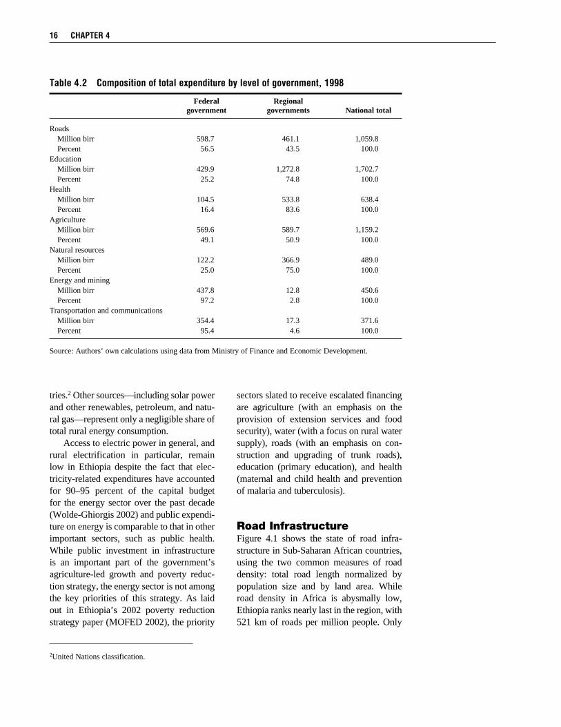
tries.2 Other sources—including solar power and other renewables, petroleum, and natu-ral gas—represent only a negligible share of total rural energy consumption. Access to electric power in general, and rural electrification in particular, remain low in Ethiopia despite the fact that elec-tricity-related expenditures have accounted for 90–95 percent of the capital budget for the energy sector over the past decade (Wolde-Ghiorgis 2002) and public expendi-ture on energy is comparable to that in other important sectors, such as public health. While public investment in infrastructure is an important part of the government’s agriculture-led growth and poverty reduc-tion strategy, the energy sector is not among the key priorities of this strategy. As laid out in Ethiopia’s 2002 poverty reduction strategy paper (MOFED 2002), the priority
sectors slated to receive escalated financing are agriculture (with an emphasis on the provision of extension services and food security), water (with a focus on rural water supply), roads (with an emphasis on con-struction and upgrading of trunk roads), education (primary education), and health (maternal and child health and prevention of malaria and tuberculosis).
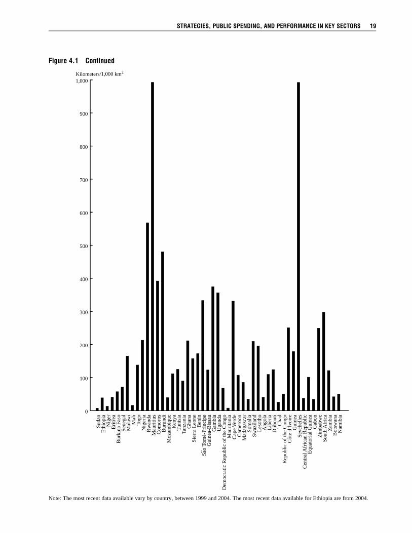
Road InfrastructureFigure 4.1 shows the state of road infra-structure in Sub-Saharan African countries, using the two common measures of road density: total road length normalized by population size and by land area. While road density in Africa is abysmally low, Ethiopia ranks nearly last in the region, with 521 km of roads per million people. Only
16 cHapter 4
2United Nations classification.
table 4.2 composition of total expenditure by level of government, 1998
Federal Regional government governments National total
Roads Million birr 598.7 461.1 1,059.8 Percent 56.5 43.5 100.0Education Million birr 429.9 1,272.8 1,702.7 Percent 25.2 74.8 100.0Health Million birr 104.5 533.8 638.4 Percent 16.4 83.6 100.0Agriculture Million birr 569.6 589.7 1,159.2 Percent 49.1 50.9 100.0Natural resources Million birr 122.2 366.9 489.0 Percent 25.0 75.0 100.0Energy and mining Million birr 437.8 12.8 450.6 Percent 97.2 2.8 100.0Transportation and communications Million birr 354.4 17.3 371.6 Percent 95.4 4.6 100.0
Source: Authors’ own calculations using data from Ministry of Finance and Economic Development.

strategies, public spending, and performance in key sectors 17
Sudan has a lower population-normalized road density. When road density is mea-sured with respect to land area, Ethiopia still ranks ninth from last (with Sudan again last) among African countries, with 36 km of roads per 1,000 km2. This current state of road infrastructure, in fact, follows a drastic increase in public investment in roads since the mid-1990s. This resulted in an expan-sion of the total road network in Ethiopia by 35 percent. As of 2005 about half of Ethio-pia’s road network is made up of trunk and link roads administered by a federal agency, the Ethiopian Roads Authority. The remain-der are the so-called rural roads, which are administered by regional agencies, the rural roads authorities. Public investment and other policies regarding roads are laid out in the Road Sector Development Program (RSDP), de-veloped by the Ethiopian Roads Authority in 1997. The RSDP outlines a 10-year strategy for developing road infrastructure. During the first phase, from 1997 to 2002, road-building projects were to give priority (in this order) to providing improved ac-cess to ports, as well as existing and new resource areas and food-deficit areas, and to maintaining a degree of equity between the regions in terms of transport infrastructure. Given these priorities, a relatively large share of the capital expenditures were allo-cated for asphalt and gravel roads. However, the 34 percent increase in unpaved roads in the latter half of the 1990s was much higher than the increase in paved roads (7 percent) over the same period (MOFED 2002). The second phase of the RSDP, from 2003 to 2007, was designed to address the low level of road connectivity among the re-gions. The main roads typically radiate from Addis Ababa to the various regions, but travel between regional towns is difficult. The second phase of the RSDP also empha-sized the development of village rural roads, which were more likely to immediately ben-efit poor populations. Village-level associa-tions were assigned the task of proposing and implementing road projects. However,
institutions at all administrative levels— kebeles (peasant associations), weredas, re-gions, and the federal level—are expected to be involved in the various stages of rural road development. Public investment in roads as a share of spending in the agricultural, social, and infra- structure sectors increased significantly, beginning with the change of government in 1991. As seen in Table 4.1, this share of spending in these sectors rose from 3–5 percent in the 1980s to 15–20 percent in the 1990s. Indeed the relative increase in spend-ing on road construction is unrivaled by the increase in any of the other agricultural, social, or infrastructure sectors in Ethiopia. Table 4.3 shows the geographic distri- bution of road spending. When the share of each region’s (capital) expenditure, ex-pressed relative to the total capital spending of all regions, is compared with its share of the population, it becomes evident that the capital city-state Addis Ababa and the more marginal areas of Beneshangul-Gumuz, Gambela, and (to some extent) Afar have allocated resources to roads well beyond their population shares. Tables 4.4 and 4.5 show road density by region, with Table 4.4 showing density over time and Table 4.5 showing these data dis-aggregated by road type. A comparison of Tables 4.4 and 4.5 with Table 4.3 shows that in the case of the road sector, the geographic distribution of sectoral performance may be broadly aligned with the expenditure dis-tribution. Road density, measured as kilo- meters of roads per 1,000 people, was con-sistently highest in Gambela and second highest in either Beneshangul-Gumuz or Afar, depending on the year. However, while population-based road density was highest in the marginal regions, it was lowest (or, to be precise, zero) for asphalted roads in regions such as Beneshangul- Gumuz, Gambela, and Somale. Interest-ingly and surprisingly, Table 4.5 shows that it was highest for Afar, possibly due to the low population density in this pastoral region. When road density was measured in

18 cHapter 4
Kilometers/million population
0
Suda
n
16,000
14,000
12,000
10,000
8,000
6,000
4,000
2,000
22,000
Eth
iopi
aN
iger
Eri
trea
Bur
kina
Fas
oSe
nega
lM
alaw
iM
ali
Togo
Nig
eria
Rw
anda
Mau
ritiu
sC
omor
osB
urun
diM
ozam
biqu
eK
enya
Tun
isia
Tanz
ania
Gha
naSi
erra
Leo
neB
enin
Sao
Tom
é-Pr
inci
peG
uine
a-B
issa
uG
ambi
aU
gand
aD
emoc
ratic
Rep
ublic
of
the
Con
goM
auri
tani
aC
ape
Ver
deC
amer
oon
Mad
agas
car
Som
alia
Swaz
iland
Les
otho
Ang
ola
Lib
eria
Djib
outi
Cha
dR
epub
lic o
f th
e C
ongo
Côt
e d’
lvoi
reG
uine
aSe
yche
lles
Cen
tral
Afr
ican
Rep
ublic
Equ
ator
ial G
uine
aG
abon
Zim
babw
eSo
uth
Afr
ica
Zam
bia
Bot
swan
aN
amib
ia
18,000
20,000
~
figure 4.1 road density in ethiopia and sub-saharan african countries
Source: World Bank (2007).Note: The most recent data available vary by country, between 1999 and 2004. The most recent data available for Ethiopia are from 2004.
strategies, public spending, and performance in key sectors 19
Kilometers/1,000 km2
0
Suda
n
700
600
500
400
300
200
100
1,000
Eth
iopi
aN
iger
Eri
trea
Bur
kina
Fas
oSe
nega
lM
alaw
iM
ali
Togo
Nig
eria
Rw
anda
Mau
ritiu
sC
omor
osB
urun
diM
ozam
biqu
eK
enya
Tun
isia
Tanz
ania
Gha
naSi
erra
Leo
neB
enin
Gui
nea-
Bis
sau
Gam
bia
Uga
nda
Dem
ocra
tic R
epub
lic o
f th
e C
ongo
Mau
rita
nia
Cap
e V
erde
Cam
eroo
nM
adag
asca
rSo
mal
iaSw
azila
ndL
esot
hoA
ngol
aL
iber
iaD
jibou
tiC
had
Rep
ublic
of
the
Con
goC
ôte
d’lv
oire
Gui
nea
Seyc
helle
sC
entr
al A
fric
an R
epub
licE
quat
oria
l Gui
nea
Gab
onZ
imba
bwe
Sout
h A
fric
aZ
ambi
aB
otsw
ana
Nam
ibia
800
900
Sao
Tom
é-Pr
inci
pe~
figure 4.1 continued
Note: The most recent data available vary by country, between 1999 and 2004. The most recent data available for Ethiopia are from 2004.

table 4.3 capital and recurrent road infrastructure expenditures by region, 1998
Addis Beneshangul- Regional Ababa Afar Amhara Gumuz Gambela Harari Oromia SNNP Somale Tigray total
Capital Million birr 117.9 17.7 78.3 23.5 13.8 0.0 98.5 48.4 24.0 20.6 442.8 Percent 26.6 4.0 17.7 5.3 3.1 0.0 22.2 10.9 5.4 4.7 100.0Recurrent Million birr 8.4 0.0 3.9 0.2 0.0 0.0 4.7 0.0 0.0 1.1 18.3 Percent 46.0 0.0 21.1 1.2 0.0 0.0 25.9 0.0 0.0 5.8 100.0Recurrent as percent of total 6.7 0.0 4.7 0.9 0.0 0.0 4.6 0.0 0.0 4.9 4.0Population Thousands 2,570 1,243 16,748 551 216 166 23,023 12,903 3,797 3,797 65,344 Percent 3.9 1.9 25.6 0.8 0.3 0.3 35.2 19.7 5.8 5.8 100.0
Source: Authors’ own calculations using data from Ministry of Finance and Economic Development. Data for Dire Dawa were not available.Note: SNNP—Southern Nations, Nationalities, and Peoples.
table 4.4 density of all-weather roads, selected years
Kilometers per 1,000 persons Kilometers per 1,000 km2
Region 1995 1996 1997 2003 2004 1995 1996 1997 2003 2004
Addis Ababa n.a. n.a. n.a. 0.7 0.7 n.a. n.a. n.a. 3,659.4 3,849.7Afar 0.7 1.0 1.0 1.5 1.6 8.7 12.6 12.7 21.3 23.7Amhara 0.2 0.3 0.3 0.4 0.4 20.8 32.1 32.9 46.0 48.5Beneshangul-Gumuz 0.8 0.9 0.8 2.5 3.1 8.0 8.4 8.4 29.1 36.4Dire Dawa n.a. n.a. n.a. 0.4 0.5 n.a. n.a. n.a. 93.6 126.8Gambela 1.7 4.8 4.7 5.9 6.6 12.6 36.3 36.3 52.1 60.5Harari n.a. n.a. n.a. 0.4 0.7 n.a. n.a. n.a. 188.8 315.7Oromia 0.4 0.5 0.5 0.4 0.4 22.5 34.4 34.4 29.8 31.0SNNP 0.2 0.3 0.3 0.4 0.4 19.5 25.2 26.5 43.8 46.8Somale 0.4 0.4 0.4 0.8 0.8 3.8 4.0 4.2 10.1 10.6Tigray 0.2 0.5 0.5 0.6 0.7 12.0 29.1 30.0 44.1 51.0Ethiopia 0.3 0.4 0.4 0.5 0.5 14.0 21.2 21.6 30.1 32.5
Source: Central Statistical Authority (1995, 1996, 1997); Ethiopian Roads Authority.Note: n.a.—Not available; SNNP—Southern Nations, Nationalities, and Peoples.
table 4.5 road density by road type, 2003
Kilometers per 1,000 persons Kilometers per 1,000 km2
Asphalt Gravel Rural Asphalt Gravel RuralRegion roads roads roads All roads roads roads roads All roads
Addis Ababa 0.155 0.550 0.000 0.706 804.948 2,854.424 0.000 3,659.372Afar 0.539 0.277 0.673 1.489 7.720 3.971 9.648 21.340Amhara 0.049 0.112 0.230 0.391 5.739 13.208 27.010 45.957Beneshangul-Gumuz 0.000 1.302 1.243 2.540 0.000 14.910 14.238 29.148Dire Dawa 0.075 0.244 0.078 0.395 17.650 57.528 18.446 93.624Gambela 0.000 2.661 3.199 5.860 0.000 23.650 28.437 52.087Harari 0.105 0.133 0.179 0.418 47.462 60.152 81.218 188.832Oromia 0.073 0.117 0.194 0.383 5.735 9.190 15.196 30.121SNNP 0.031 0.153 0.245 0.428 3.600 18.090 28.913 50.603Somale 0.000 0.292 0.523 0.815 0.000 3.632 6.511 10.143Tigray 0.060 0.313 0.249 0.622 4.253 22.222 17.672 44.146Ethiopia 0.065 0.184 0.255 n.a. 3.977 11.288 15.661 167.408
Source: Ethiopian Roads Authority (road length); Central Statistical Authority (population data); dataset for World Bank (2005b) (land area).Note: n.a.—Not available; SNNP—Southern Nations, Nationalities, and Peoples.
terms of area (kilometers of roads per 1,000 km2), Addis Ababa, followed by the city-state of Harari, had the highest density.3
AgricultureAs discussed earlier, agriculture is at the heart of the ADLI strategy and is expected to fuel economic growth and poverty reduc-tion. Given such a focus on the agricultural sector, one would expect to see strong re-source allocation to agriculture since 1993, when ADLI was first conceived. Indeed, despite fluctuations, real agricultural expen-diture has been increasing since then (Table 4.6). Through the decentralization and in-tensification of extension services, which is one of the key features of ADLI, expen-diture on agricultural extension approxi-mately doubled over the 1990s (although it continues to constitute a rather small share of agricultural spending). Table 4.6 also suggests that, over time, allocations have shifted somewhat away from spending related to natural resources and the environment in favor of agriculture. With the country heavily dependent on both agriculture and its natural resource base, and given the intimate relationship between the agricultural sector and the environ- mental and natural resource sector, it is not immediately apparent how the government should balance its spending between these two areas. The noticeable shift of expen- ditures in favor of the agricultural sector appears to reflect the increasingly high priority accorded by the government to the provision of agricultural services and technology. Regarding the administrative sources of spending in the 1990s—that is, the share of expenditures executed by subnational
administrative units versus the federal government—the last row of Table 4.6 shows that regions handled the majority of expenditures in the agricultural and natural resources sector. Despite progressive de-centralization in Ethiopia, this share has de-clined in recent years. World Bank (2008) discusses this trend in greater detail. A regional breakdown of real per capita expenditure on agriculture over this period is presented in Table 4.7. For most of the regions, agricultural spending was less than 30 birr per capita. Some of the highest ex-penditures, however, took place in the rela-tively urbanized regions of Addis Ababa and Harari. The Gambela region spent by far the largest amount per capita in agricul-ture; this no doubt reflects the dramatically higher per capita public budget and federal transfers to Gambela. While the national figure for agricultural spending as a whole moderately increased during this period, high variation was seen at the regional level, meaning that no particular regional spend-ing pattern is readily discernable. The regional distribution of land produc-tivity (one indicator of agricultural perfor-mance) is illustrated in Table 4.8. Thanks to its favorable agroecological conditions, Gambela had the highest yield levels by far, whereas the arid regions of Afar, Dire Dawa, Harari, and Somale had the lowest. In particular the pastoral regions of Afar and Somale rely much more heavily on livestock breeding as the main economic activity, hence these results are not unexpected. One could naturally expect there to be a lag period between the inception of agricul-tural expenditures and the point at which results might be observed in terms of agri- cultural performance. Even given this, how-ever, it appears that over the 1990s agricul-
strategies, public spending, and performance in key sectors 21
3This is despite the fact that these road data do not capture municipal roads, but only rural and interregional roads. For example, the total road network of the SNNP region does not include the length of roads managed by the cit-ies within SNNP. However, the very high density of interregional and other nonmunicipal roads passing through commercially important towns such as Addis Ababa and Harari contributes to these city-states’ high figures for road infrastructure.

22 cHapter 4
table 4.6 total national expenditure on agriculture and natural resources, 1993–2000 (millions, constant 1995 birr)
Expenditure category 1993 1994 1995 1996 1997 1998 1999 2000
Ministry of Agriculture 196.2 224.9 304.1 363.5 373.1 417.1 388.3 451.0Agricultural research 78.8 61.5 15.8 31.8 74.0 98.2 105.1 170.1Agricultural extension 10.7 9.8 18.5 16.9 23.9 26.0 22.2 19.4Other agricultural services 306.1 223.3 311.3 296.9 181.2 553.9 417.6 303.8Seed — — 0.3 0.4 0.8 2.7 1.9 3.2Fertilizer — — — 0.5 0.6 0.7 0.7 9.8Coffee and Tea Authority 60.2 63.4 24.8 19.5 5.4 7.3 33.6 27.3Livestock — — — — — 1.6 1.5 2.0Cooperatives development — — — — — — — 3.4Integrated development — — — — — 0.6 1.4 2.2Rural infrastructure 16.7 — — — 44.6 57.9 — —Other agricultural expenditures — — — — — — — 3.2Ministry of Water 69.4 109.4 61.5 61.3 55.5 57.6 65.5 93.9Water supply — 248.9 220.5 345.0 346.8 293.4 254.4 196.4Other water expenditures — — — 119.2 92.0 134.5 49.1 122.2Environment — — — 1.1 1.3 1.6 1.8 3.1Biodiversity — — — — 1.2 1.5 1.6 4.2Other natural resource expenditures 411.8 262.1 202.7 127.5 51.7 — — —Total 1,149.9 1,203.4 1,159.4 1,383.6 1,252.2 1,654.5 1,344.6 1,415.3Percent subnational 69.8 63.4 71.0 79.5 76.2 58.0 58.4 58.1
Source: Authors’ own calculations using data from Ministry of Finance and Economic Development.Notes: “Ministry of Agriculture” refers mostly to administrative and personnel expenditures of the ministry. There was little information in the data provided on what constituted “Other agricultural services.” Refer to World Bank (2008) for a more in-depth discussion of the composition and pattern of public spending on agriculture and rural development in Ethiopia. — indicates the category was not recorded for this year.
table 4.7 real per capita regional expenditure on agricultural and natural resources, 1993–2000 (birr)
Region 1993 1994 1995 1996 1997 1998 1999 2000
Addis Ababa 11.76 22.43 50.25 61.91 58.72 44.64 29.66 13.31Afar 32.29 16.57 16.09 6.47 18.27 61.27 33.63 24.29Amhara 8.25 10.40 10.40 11.27 12.12 11.96 9.10 9.69Beneshangul-Gumuz 18.87 23.90 19.84 11.29 14.66 43.24 56.86 36.78Dire Dawa 14.42 18.32 17.52 14.16 15.26 14.91 8.39 7.86Gambela 52.58 77.29 100.29 134.37 48.88 37.11 35.94 34.80Harari 4.49 58.67 32.46 52.92 50.46 21.48 16.63 104.97Oromia 10.30 14.76 12.79 20.28 14.93 12.08 10.77 15.50SNNP 8.00 12.80 13.16 12.85 10.29 15.25 7.54 7.91Somale 3.42 10.47 19.18 18.54 14.58 11.94 25.83 10.65Tigray 17.67 19.04 13.80 34.80 26.91 17.18 12.98 12.91Ethiopia 16.63 22.08 20.64 23.89 20.97 26.88 21.19 21.68
Source: Authors’ own calculations using data from Ministry of Finance and Economic Development.Note: SNNP—Southern Nations, Nationalities, and Peoples.

tural productivity has not responded to investments. It may therefore be necessary to empirically extend this descriptive analy-sis in order to examine other indicators of agricultural performance, further dissect the provision of public services within the agricultural subsectors, and monitor per-formance indicators within the agricultural sector over a longer period.
EducationThe rural literacy rate in Ethiopia (for the population 10 years old and above) started from a very low baseline in the early 1990s and has since shown improvement both in levels and in terms of urban-rural and
gender disparities. In 1999 the rural and urban literacy rates were 22 and 70.4 per-cent, respectively (MOFED 2002), which in turn had improved from 16 and 70 per-cent, respectively, only two years earlier. The gender gap in rural literacy improved somewhat during this period, with the ratio of female literacy rate to male literacy rate rising from 0.28 to 0.33. However, as of 2002, Ethiopia remained far behind other poor countries worldwide in terms of edu-cational outcomes (Table 4.9). Ethiopia has made some important progress when one considers the longer view and examines intermediate outcomes in the education sector. Over the past 10 or so years, educational coverage at all levels
strategies, public spending, and performance in key sectors 23
table 4.9 literacy rate, 1990 and 2002 (percent of 15-year-olds and above)
Male Female Gender gap
1990 2002 Increase 1990 2002 Increase 1990 2002
Ethiopia 37 49 12 20 34 14 17 15South Asia 59 67 8 34 44 10 25 23Sub-Saharan Africa 60 71 11 40 56 16 20 15Low income 64 72 8 42 53 11 22 19
Source: World Bank (2005e).
table 4.8 yield of annual crops by region, 1995–2000 (quintals per hectare)
Region 1995 1996 1997 1998 1999 2000
Addis Ababa 14.9 12.0 13.0 10.0 10.3 12.6Afar 7.9 13.2 7.3 n.a. 12.9 2.5Amhara 9.8 10.2 8.9 9.5 9.4 9.5Beneshangul-Gumuz 11.1 10.5 11.4 11.3 10.7 10.2Dire Dawa 5.9 11.6 7.4 10.5 10.0 9.2Gambela 22.6 17.4 19.3 20.5 19.3 21.5Harari 10.4 9.7 7.4 8.5 8.8 7.5Oromia 13.1 13.2 12.2 11.7 12.1 12.9SNNP 13.3 13.5 12.6 10.6 10.6 11.9Somale 7.1 7.3 9.8 5.7 4.7 7.6Tigray 11.0 12.3 8.9 10.8 11.1 9.8Ethiopia 11.7 11.9 10.7 10.7 10.8 11.2
Source: Calculated using data from the Central Statistical Authority’s Agricultural Sample Surveys, 1995–2000.Note: n.a.—Not available; SNNP—Southern Nations, Nationalities, and Peoples.

has experienced a sustained increase. The greatest success was achieved at the primary level, where the gross enrollment ratio more than tripled from 20 percent in 1993 to 62 percent in 2001. Other levels also showed increases, with the enrollment ratio in sec-ondary education increasing from 8 percent to 12 percent, and that in tertiary education increasing from 0.5 percent to 1.7 percent (World Bank 2005a; see also Table 4.10).
Unfortunately these improvements in coverage have been accompanied by a sus-tained deterioration in educational quality. The national average pupil-to-teacher ratio (PTR) increased steadily over the 1990s and into the new millennium (Table 4.11), with the most serious effects seen in rural areas. For example, the PTR in 1994 was 32 in rural areas and 34 in urban areas. By 2001 the PTR in rural areas had more than
24 cHapter 4
table 4.10 primary school (grades 1–8) gross enrollment ratio, 1994–2003
Region 1994 1995 1996 1997 1998 1999 2000 2001 2002 2003
Addis Ababa 84.9 82.9 80.3 82.0 84.7 91.4 118.3 128.4 135.4 142.6Afar 8.4 8.4 8.4 8.4 7.1 9.1 11.5 12.6 13.8 14.8Amhara 17.9 22.3 28.0 34.6 40.4 46.8 53.3 58.1 58.5 61.8Beneshangul-Gumuz 35.4 42.8 48.6 69.9 74.9 81.8 88.5 89.1 98.4 100.5Dire Dawa 41.0 41.6 50.7 58.9 60.0 62.4 75.7 80.2 78.6 83.2Gambela 53.9 50.4 66.3 83.5 89.1 93.7 95.8 102.7 124.6 106.6Harari 53.4 54.9 65.6 77.1 90.0 96.2 105.3 107.5 105.0 104.5Oromia 21.2 26.0 30.8 39.6 45.0 51.6 57.9 62.4 66.9 72.7SNNP 28.8 38.4 44.4 55.7 56.8 59.8 63.8 67.5 71.8 74.2Somale 11.6 11.6 11.6 11.6 8.0 8.3 10.6 13.1 15.1 15.1Tigray 43.7 45.0 45.1 56.1 58.4 63.5 73.9 77.6 73.7 80.6Ethiopia 26.2 30.1 34.7 41.8 45.8 51.0 57.4 61.6 64.4 68.4
Source: Ministry of Education.Notes: The primary gross enrollment ratio is defined as the ratio between all students enrolled in primary school and the population in the of-ficial age range for that cycle. In Ethiopia the age range for primary schooling is 7–14 years. Thus enrollment of students who are outside the official age bracket can lead to this ratio exceeding 100 percent. SNNP—Southern Nations, Nationalities, and Peoples.
table 4.11 primary school (grades 1–8) pupil-to-teacher ratio, selected years
Region 1992 1995 1999 2000 2001 2002 2003
Addis Ababa 49 51 46 45 38 41 39Afar 29 23 28 29 31 29 32Amhara 20 33 62 67 70 70 71Beneshangul-Gumuz 18 38 50 50 52 49 51Dire Dawa 33 38 43 44 41 40 41Gambela 22 35 35 36 38 39 48Harari 26 36 26 23 24 27 24Oromia 21 32 53 60 66 68 72SNNP 28 51 61 63 66 67 67Somale 13 21 37 35 44 52 52Tigray 51 47 62 67 69 59 55Ethiopia 27 38 56 60 63 64 65
Source: Ministry of Education.Note: SNNP—Southern Nations, Nationalities, and Peoples.

doubled to 73, whereas the urban ratio had increased to only 48. This has dramatically increased the burden on teachers in rural areas, making it more difficult to encourage graduates from cities and towns to take rural teaching positions.
In 1994 the government of Ethiopia adopted the New Education and Training Policy. This policy sought to change the existing structure of the education system, which was modeled after Western education systems and was perceived by the govern-ment as being inappropriate for the realities of Ethiopia. The new system defined pri-mary education as grades 1–8, thus putting pressure on school capacities in the higher secondary grades (standardized testing was not administered prior to grade 8). This prompted the government to drastically in-crease enrollment barriers to the 11th grade, effective with the 2001/02 school year. The 1994 reform also placed new em-phasis on the expansion of technical and vocational education and training (TVET) and required the use of local languages for primary instruction.
The policy focus on TVET translated into a substantial increase of public spend-ing for this subsector relative to overall ed- ucation spending. While recurrent educa- tion expenditures increased by 78 percent from 1993 to 2001, TVET expenditures in-
creased more than 12-fold or by 1,120 per-cent (World Bank 2005a). Recurrent expen-ditures for higher education also increased disproportionately to the overall rise in spending, more than tripling during this period. While spending at the primary level constituted the largest share of education expenditure, it grew more slowly than overall expenditure, increasing by only 40 percent from 1993 to 2001. Possibly to rectify this imbalance, the government’s 2002 poverty reduction strategy stated that improvement of access to primary educa-tion would be the top priority within the education sector.
HealthAlthough Ethiopia has shown modest and gradual improvements on a range of health indicators, these indicators remain at very low levels overall. Child mortality has im-proved from 269 per 1,000 live births in 1960 to 204 in 1990 to 170 in 2002. How-ever, in order for Ethiopia to meet the Millennium Development Goals for health this figure must be halved over the next decade (World Bank 2004). Immunization rates have been subject to large swings over the past few decades, with downswings often coinciding with periods of unrest and war. As of 2002 the immunization rate was
strategies, public spending, and performance in key sectors 25
table 4.12 immunization and child mortality rates for ethiopia and selected african countries, 2002
Immunization rate Mortality rate (percent 1–2 yrs) (per 1,000 live births)
GDP Diphtheria- Under per capita pertussis-tetanus Measles Infant 5 years old
Ethiopia 124 56 52 114 171Malawi 157 64 69 113 182Sierra Leone 165 50 60 165 284Tanzania 207 89 89 104 165Chad 232 40 55 117 200Ghana 429 80 81 60 97
Source: World Bank (2005e).
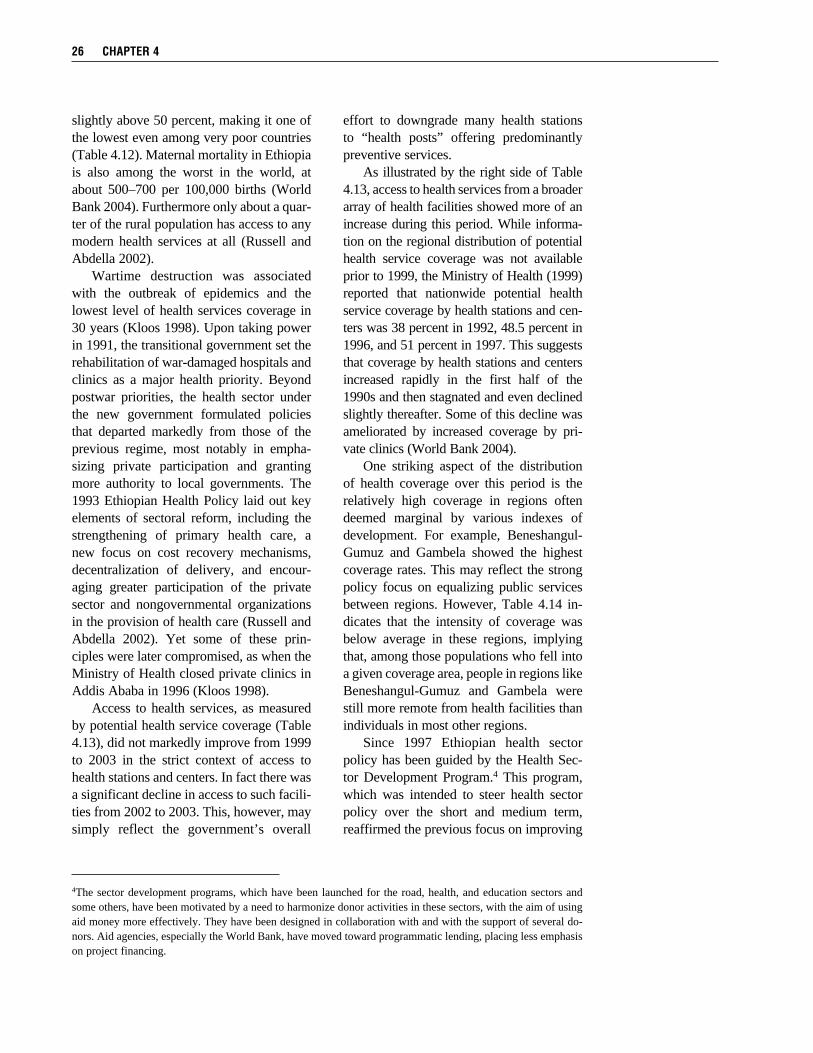
slightly above 50 percent, making it one of the lowest even among very poor countries (Table 4.12). Maternal mortality in Ethiopia is also among the worst in the world, at about 500–700 per 100,000 births (World Bank 2004). Furthermore only about a quar-ter of the rural population has access to any modern health services at all (Russell and Abdella 2002). Wartime destruction was associated with the outbreak of epidemics and the lowest level of health services coverage in 30 years (Kloos 1998). Upon taking power in 1991, the transitional government set the rehabilitation of war-damaged hospitals and clinics as a major health priority. Beyond postwar priorities, the health sector under the new government formulated policies that departed markedly from those of the previous regime, most notably in empha-sizing private participation and granting more authority to local governments. The 1993 Ethiopian Health Policy laid out key elements of sectoral reform, including the strengthening of primary health care, a new focus on cost recovery mechanisms, decentralization of delivery, and encour-aging greater participation of the private sector and nongovernmental organizations in the provision of health care (Russell and Abdella 2002). Yet some of these prin-ciples were later compromised, as when the Ministry of Health closed private clinics in Addis Ababa in 1996 (Kloos 1998). Access to health services, as measured by potential health service coverage (Table 4.13), did not markedly improve from 1999 to 2003 in the strict context of access to health stations and centers. In fact there was a significant decline in access to such facili-ties from 2002 to 2003. This, however, may simply reflect the government’s overall
effort to downgrade many health stations to “health posts” offering predominantly preventive services. As illustrated by the right side of Table 4.13, access to health services from a broader array of health facilities showed more of an increase during this period. While informa-tion on the regional distribution of potential health service coverage was not available prior to 1999, the Ministry of Health (1999) reported that nationwide potential health service coverage by health stations and cen-ters was 38 percent in 1992, 48.5 percent in 1996, and 51 percent in 1997. This suggests that coverage by health stations and centers increased rapidly in the first half of the 1990s and then stagnated and even declined slightly thereafter. Some of this decline was ameliorated by increased coverage by pri-vate clinics (World Bank 2004). One striking aspect of the distribution of health coverage over this period is the relatively high coverage in regions often deemed marginal by various indexes of development. For example, Beneshangul-Gumuz and Gambela showed the highest coverage rates. This may reflect the strong policy focus on equalizing public services between regions. However, Table 4.14 in-dicates that the intensity of coverage was below average in these regions, implying that, among those populations who fell into a given coverage area, people in regions like Beneshangul-Gumuz and Gambela were still more remote from health facilities than individuals in most other regions. Since 1997 Ethiopian health sector policy has been guided by the Health Sec-tor Development Program.4 This program, which was intended to steer health sector policy over the short and medium term, reaffirmed the previous focus on improving
26 cHapter 4
4The sector development programs, which have been launched for the road, health, and education sectors and some others, have been motivated by a need to harmonize donor activities in these sectors, with the aim of using aid money more effectively. They have been designed in collaboration with and with the support of several do-nors. Aid agencies, especially the World Bank, have moved toward programmatic lending, placing less emphasis on project financing.
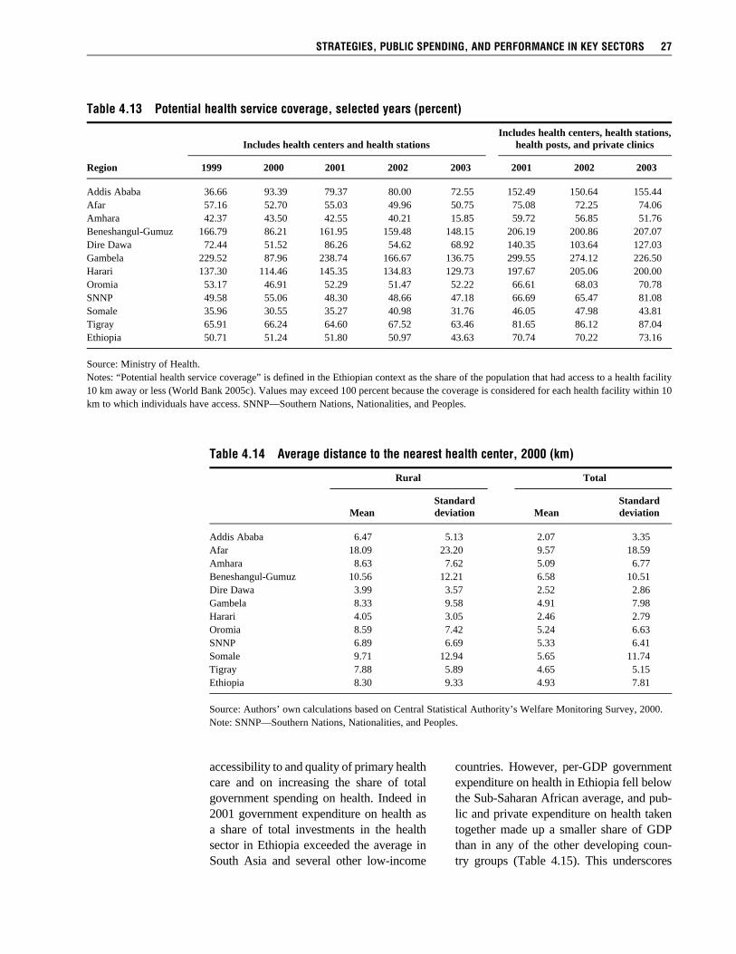
strategies, public spending, and performance in key sectors 27
table 4.13 potential health service coverage, selected years (percent)
Includes health centers, health stations, Includes health centers and health stations health posts, and private clinics
Region 1999 2000 2001 2002 2003 2001 2002 2003
Addis Ababa 36.66 93.39 79.37 80.00 72.55 152.49 150.64 155.44Afar 57.16 52.70 55.03 49.96 50.75 75.08 72.25 74.06Amhara 42.37 43.50 42.55 40.21 15.85 59.72 56.85 51.76Beneshangul-Gumuz 166.79 86.21 161.95 159.48 148.15 206.19 200.86 207.07Dire Dawa 72.44 51.52 86.26 54.62 68.92 140.35 103.64 127.03Gambela 229.52 87.96 238.74 166.67 136.75 299.55 274.12 226.50Harari 137.30 114.46 145.35 134.83 129.73 197.67 205.06 200.00Oromia 53.17 46.91 52.29 51.47 52.22 66.61 68.03 70.78SNNP 49.58 55.06 48.30 48.66 47.18 66.69 65.47 81.08Somale 35.96 30.55 35.27 40.98 31.76 46.05 47.98 43.81Tigray 65.91 66.24 64.60 67.52 63.46 81.65 86.12 87.04Ethiopia 50.71 51.24 51.80 50.97 43.63 70.74 70.22 73.16
Source: Ministry of Health.Notes: “Potential health service coverage” is defined in the Ethiopian context as the share of the population that had access to a health facility 10 km away or less (World Bank 2005c). Values may exceed 100 percent because the coverage is considered for each health facility within 10 km to which individuals have access. SNNP—Southern Nations, Nationalities, and Peoples.
table 4.14 average distance to the nearest health center, 2000 (km)
Rural Total
Standard Standard Mean deviation Mean deviation
Addis Ababa 6.47 5.13 2.07 3.35Afar 18.09 23.20 9.57 18.59Amhara 8.63 7.62 5.09 6.77Beneshangul-Gumuz 10.56 12.21 6.58 10.51Dire Dawa 3.99 3.57 2.52 2.86Gambela 8.33 9.58 4.91 7.98Harari 4.05 3.05 2.46 2.79Oromia 8.59 7.42 5.24 6.63SNNP 6.89 6.69 5.33 6.41Somale 9.71 12.94 5.65 11.74Tigray 7.88 5.89 4.65 5.15Ethiopia 8.30 9.33 4.93 7.81
Source: Authors’ own calculations based on Central Statistical Authority’s Welfare Monitoring Survey, 2000.Note: SNNP—Southern Nations, Nationalities, and Peoples.
accessibility to and quality of primary health care and on increasing the share of total government spending on health. Indeed in 2001 government expenditure on health as a share of total investments in the health sector in Ethiopia exceeded the average in South Asia and several other low-income
countries. However, per-GDP government expenditure on health in Ethiopia fell below the Sub-Saharan African average, and pub-lic and private expenditure on health taken together made up a smaller share of GDP than in any of the other developing coun-try groups (Table 4.15). This underscores

the relatively significant role that public funds play in the financing of Ethiopia’s health sector. In absolute terms, spend-ing on health per person in Ethiopia falls far short of expenditures in Africa, South Asia, and the low-income countries. Health expenditures are $3 per capita per annum in Ethiopia, which is between one-seventh and one-tenth of comparable expenditures in other low-income economies. In the implementation of Ethiopia’s decentralization policy, the devolution of resource allocation responsibility to the lower tiers of government was most exten-sive for the social sectors, including health. Accordingly the regions accounted for over 87 percent of government recurrent expen-diture and nearly all (99 percent) of capital expenditure in 2001. With the deepening of decentralization beginning in 2002, part of the regional health budgets were passed down to the weredas. As seen in the de-centralization of spending responsibility in
other sectors, some problems were associ-ated with the devolution. For example, the weredas were not fully capable of maintain-ing facilities, did not have adequate staffing (despite the continued deployment of health personnel from the regions), and faced chal-lenges in coordinating with other weredas for services and drug distribution activities spanning a wider geographic space. In the following chapters we build on this descriptive overview, expanding the inquiry to examine how public expenditure in key sectors may have differentially af-fected the welfare of rural households. The next chapter sets the stage by providing the conceptual context for how public spending may contribute to rural household incomes by affecting the productivity of household private assets. We also discuss the possibil-ity of expenditure policy itself being influ-enced by sector-specific levels of develop-ment, and what this implies for econometric identification in the analysis.
28 cHapter 4
table 4.15 Health expenditures in ethiopia and other low-income country groups, 2001
percent of GDP
Public as percent Expenditure Total Public of total expenditure per capita ($)
Ethiopia 4 1 41 3South Asia 5 1 22 22Low income 4 1 26 23Sub-Saharan Africa 6 3 41 29
Source: World Bank (2005e).
Expenditure as percent of GDP

C H A P T E R 5
Conceptual Framework of Public Spending, Public Services, and Private Assets
F igure 5.1 is an illustration of the framework that underlies our analysis of the effect of public expenditures on rural welfare. This analysis comprises three stages. The first is represented by the upper half of the illustration and the links shown by the solid
arrows. It highlights the role of access to public services in determining the welfare of rural households, incorporating the way in which public services and sector-specific outcomes may contribute directly to that welfare; they may also contribute indirectly by increasing the pro-ductivity of households’ private assets. The second stage of our analysis is summarized by the bottom half of the figure. This shows how public services and infrastructure or sector-specific performance is itself determined by the amount of public financial resources committed to the sectors (dashed arrows). The final stage of the analysis, represented by the whole figure, draws on the pathways captured by the prior two stages to show how public expenditure af-fects rural welfare. When assessing how access to different types of public services may affect household well-being, and how public expenditure leads to public services and infrastructure, several issues affecting the transformation of public financial resources into sectoral outcomes and household welfare must be considered. First, access to public services can have both direct and indirect effects on household welfare, as indicated by the thin solid arrows in Figure 5.1. The direct effects include improve-ments in well-being that are usually not captured by monetary measures of welfare, such as the value of household expenditure or income. Ferroni and Kanbur (1992) incorporated non- monetary measures in designing a framework for poverty-oriented public expenditure allocation. For example, improved sanitation arising from public subsidies for the construction of household latrines directly benefits individuals through the inherent desirability of improved hygiene. But direct effects can also be realized in the conventional metric of welfare. For example, public provision of unconditional “safety net” transfers directly boosts household income. Most public services, however, predominantly improve household welfare in indirect ways, by affecting the returns to, or the productivity of, households’ private assets. For exam-ple, public investment in irrigation infrastructure improves the welfare of agricultural house-holds by increasing the contribution of their agricultural assets (such as cultivable land) to production. Naturally the provision of public services may have both direct and indirect im-pacts on well-being; in the example of access to better sanitation given above, latrine subsidies offer the inherent (nonmonetary) benefits of improved hygiene, while health improvements arising from these public investments may make household members more productive. In this sense, sanitation investments indirectly affect welfare by increasing the returns to the
29

household’s labor assets. Similar mixed ef-fects are typically seen in response to better access to education.
Second, there is typically a lag between the public expenses incurred in a sector and the time when a response can be observed. The length of this lag may vary depend-ing on the type of sector-specific service indicator. For example, substantial resource investment in road construction in a given region might be expected to affect a mea-sure of road capital—say, road density—within one or two years of the investment. In contrast, education spending in a given region will not lead to an improvement in the literacy rate until several years later, because children educated today will figure into the literacy rate only after they become adults. In Figure 5.1, differences in the length of time until sectoral outcomes may be expected are suggested by the varying
thicknesses of the dashed arrows.1 The lag period will also differ for public spending within a given sector, depending on the sectoral variable. For example, education spending is expected to affect the enroll-ment ratio or school density much sooner than the literacy rate.
Third, the complementarity, mutual de-pendence, and sometimes negative external-ities (as in Ersado, Amacher, and Alwang 2004) between investments across different sectors will also affect assessment of the re-turns to public investment. This interaction across various forms of public expenditure may occur in multiple ways. At the level of expenditure policy or the budget process, the decision to spend more in a given sector implies a reduction in resources for another sector. However, resources allocated to one sector may also immediately benefit out-comes in other sectors. For example, public
30 CHAPTER 5
1The thickness of the various arrows is not intended to suggest a specific hierarchy of sectors by lag length, but only to illustrate the fact that differences in lags exist.
Rural household welfare
Households’ private assets(labor assets, land, equipment, etc.)
Road sectorperformance
Health sectorperformance
Agricultural sectorperformance
Education sectorperformance
TOTAL PUBLICEXPENDITURE
Publicexpenditure
on roads
Publicexpenditure
on agriculture
Publicexpenditureon education
Publicexpenditure
on health
Figure 5.1 Framework for the effect of public expenditures on rural household welfare

investment in road infrastructure increases road density and road quality, which in turn may reduce the transport costs for agricul-tural inputs and outputs, thus improving productivity in the agricultural sector. As demonstrated by the shaded arrows in Fig-ure 5.1, such interrelated effects are more appropriately analyzed by assessing (for ex-ample) the contribution of better road infra-structure to agricultural performance, rather than the effects of road sector expenditure on agriculture, particularly if the within- sector effects of spending are already ac-counted for. Finally, the decision to invest public re-sources in a given activity will typically be influenced by the state of affairs in the tar-get sector, as symbolized by the downward-pointing open arrows in the illustration. If the health sector is better developed in one region compared to other regions, spending may be affected in two ways: (1) a strong equity focus in expenditure policy would imply the tendency to spend less per capita on health in that region compared to other regions, or (2) a higher density of health facilities and medical staff in the region will generate a greater need for complementary health resources (such as medical supplies) compared to locations with fewer facilities per capita. Thus an expenditure policy based on resource needs would imply greater resource allocation to the more-developed region. (In this example, this would apply to expenditures complementary to facilities, rather than capital expenditure on the health centers themselves.) Furthermore a sectoral expenditure pol-icy primarily concerned with efficiency may lead to greater investments in a sector where performance indicators are already high. For example, areas with higher ag-ricultural potential (due to agroecological conditions, existing high capital base, insti-tutional structures, and so on) may also be areas in which public investment in modern inputs will generate higher returns in terms of agricultural productivity. Even if these areas are less poor than low-potential re-
gions, a sectoral strategy driven by a focus on efficiency at the sector level, and spend-ing decisions that are strongly aligned with sectoral strategies, would allocate relatively greater public resources in the agricultural sector to these better-performing areas. Naturally the size of public expenditure in a given sector depends not only on sec-toral policy, but also on the overall size of the public budget for that region (see the curved open arrows in Figure 5.1). In turn regional budgets are highly dependent on federal transfers (Table 3.1). The distribu-tion of these transfers is not neutral with respect to a region’s state of development, and this can again affect the feedback loop from development to public spending. Specifically, in the Ethiopian context, the sizes of the block grants from the federal government to the various regions are deter-mined to some extent by the government’s goal of reducing inequality across regions. Hence, as shown in Table 3.1, the per capita transfers from the federal government to Beneshangul-Gumuz, a rather underdevel-oped region, constituted 87 percent of the region’s total budget in 1997, whereas those to Addis Ababa constituted only 4 percent of that region’s budget. The simple correla-tion in per capita funds between own-source regional revenues (such as regionally col-lected taxes) and federal grants was –0.70 during this period (Table 3.1), suggesting that the equity focus of federal fiscal policy is manifested in the transfers made. This argument, taken on its own, would suggest that less-developed regions may allocate greater per capita expenditures to various sectors, ceteris paribus. However, other forces pull the relation-ship between regional sectoral develop- ment and sectoral spending in the other direction. Better-developed regions are gen-erally better equipped to generate their own revenue through taxes, user fees, and similar levies. This source of input to the regional budget therefore tends to be higher in regions with higher sectoral performance indicators. Through this link between re-
ConCEPTuAl FRAmEwoRk oF PubliC sPEnding, PubliC sERviCEs, And PRivATE AssETs 31

gional development and the region’s own revenue-raising capacity, higher sectoral development tends to contribute to greater public resources, in turn leading to higher levels of public expenditure in any given sector (holding all other factors, including federal transfers, constant). In sum, the nature of the potential re-verse feedback from sector-specific perfor-mance to the size of public expenditure is
complex. Without detailed knowledge of policy orientation, and without conclusive information about which—if any—of the policy factors discussed previously may dominate, the qualitative attributes of this feedback effect are a priori ambiguous and must be accounted for empirically. The next chapter presents the econometric strategy underlying the empirical analysis of the fea-tures we have just discussed conceptually.
32 CHAPTER 5

C H A P T E R 6
Empirical Strategy
T he conceptual framework of the previous chapter presents the three stages of analysis for tackling the research question. The empirical approaches in each of these stages are now detailed.
In the first stage, a household consumption equation specifies the effects of access to a range of public services (PS), which are allowed to operate directly (superscripted d) and indirectly (superscripted ind) to potentially enhance the productivity of private assets A. The specification is
J J
ln(cij) = a + Sfjd′DijPSij
d + Sfindj ′DijAijPSind
ij + m′Xij + eij (1) j=1 j=1
The dependent variable, ln(c), is the natural log of per-adult-equivalent household expen-diture. Dij is a dummy equal to 1 if household i is in location j. The coefficients fj may vary by area. Thus this specification permits differentiation of the effects of public service access by region, agroecological zone, or other geographic unit. The public service and private asset terms are vectors, as we are assessing the impact of multiple types of public services. The different superscripts for the public services expressions, apart from indicating the direct and indirect effects they may have on welfare, also emphasize that the vector of sectoral services that would be hypothesized to have direct effects in principle need not be identical to the vec-tor of variables with hypothesized indirect effects. X constitutes the vector of control variables, which include commonly used household characteristics, and m is the corresponding coeffi-cient vector. As usual, a is the intercept parameter and eij the error term. The second stage estimates the effects of public expenditure on services and infrastructure in selected sectors likely to be relevant to the poor. Some of the challenges faced when seeking to capture the impact of policy interventions, especially of expenditure policy, were discussed in Chapter 5. In addition public expenditure is a flow measure. In order to use such a measure to identify the effect on sectoral performance at some particular point in time, the approach to be utilized must account for the effect of public investments over time, especially in cases where the results may be expected to show a lag. Several alternative approaches have been used to determine the impact of public expendi-ture. Here we briefly discuss each, drawing on selected previous studies to provide a context for the empirical strategy used in this report. Given the concrete interest in discussing the mer- its of certain methodological questions that may inform the econometric specification (for ex-ample how the flow nature of public spending is handled, and how to account for the possible time lag in results), we will focus on studies that explicitly draw on public spending data, as
33

opposed to studies that infer public invest-ment effects from returns to physical public capital or public services. In the specific context of Ethiopia, Col-lier, Dercon, and Mackinnon (2002) used public expenditure data at the national level to compute the unit costs of increasing the quantity and quality of health care, and they then conducted simulations using these unit costs. The unit cost approach, while illustra-tive, fails to account for nonexpenditure fac-tors that may affect health capital variables, as well as the potential lag between inter-vention and outcome. However, limitations to expenditure data may necessitate this ap-proach, which was also used in Fan, Zhang, and Rao (2004) and Fan, Nyange, and Rao (2005). Similar to other studies using general equilibrium models, Agenor, Bayraktar, and El Aynaoui (2004) embedded the expendi-ture variables in a macroeconomic general equilibrium model in which public spend-ing affects total demand, government budget balance, and taxes, and is affected by the size of each revenue source. The general equilibrium approach has the advantage of assessing multiple pathways from spending to growth and poverty in an aggregate-macroeconomic framework. However, it is not clear whether the model, which depends on time series data, accounts for the lag with which spending can be expected to affect growth via the variables in the model. Gomanee, Girma, and Morrissey (2003) performed quantile regressions on cross-country panel data, in which the effect of social sector expenditure on the Human De-velopment Index was introduced contempo-raneously.1 In other words a given country’s Human Development Index for period t is regressed on expenditure in period t, along
with other control variables. Unlike the unit cost approach, regression estimation allows control of nonexpenditure influences on the outcome of interest. However, this strategy also fails to account for the possibility of lagged effects. In contrast, Devarajan, Swaroop, and Zou (1996) attempted to account for the po-tential time interval from the onset of public resource spending until the realization of economic performance. In this strategy, using a cross-country panel, a five-year moving average of GDP growth (from time t + 1 to t + 5) is the dependent variable on which public expenditure at time t is hypothesized to have an influence, and the relationship is assessed using various re-duced-form estimation methods. This struc-ture is intended to account for investment lags, and it should mitigate potential si-multaneity arising from the fact that public policy is usually driven by economic perfor-mance indicators such as growth. An alternative approach that explicitly accounts for the flow nature of public ex-penditure and the potential effects of past spending on current outcomes is akin to a distributed lag model:
tPSjt
s = l + SbqI sj,t –q + rZj + uj (2)
q=0
where I sj,t q refers to public investment in
sector s and region j undertaken at time t – q, and the tilde above the time subscript is included to indicate that equation (2) does not represent an equation with a panel struc-ture but rather one for the determination of sectoral outcomes at a particular point in time t . bq is the parameter associated with the investment variable; Zj and r are vari-able and parameter vectors, respectively,
34 CHAPTER 6
1The Human Development Index is published every year as part of the Human Development Report by the United Nations Development Programme. This index is a broader definition of well-being that goes beyond GDP and provides a composite measure of three dimensions of human development: living a long and healthy life (mea- sured by life expectancy), being educated (measured by adult literacy and enrollment rates), and having a decent standard of living (measured by purchasing power parity income).

which capture additional control determi-nants of public service performance; l is the intercept parameter; and uj is the error term. This strategy then includes investments made in each of the t time periods and al-lows differentiation of the effects of spend-ing in each year preceding the time period during which the sector-specific outcome variable is measured. One challenge to this approach is the potentially high temporal correlation of investments in a given sector and region. In particular, sectors having a high component of recurrent expenditure (for example health and education) tend to be relatively stable over time; thus, for example, Iedu
j,t1 and Iedu
j,t2 for two time periods t1 and t2 would be highly correlated, tending to wash out the significance of the investment effects. In addition there may be multiple ways to extract the parameter of interest from model (2). The question of interest here is: How much would a marginal increase in public investment in sector s affect performance in this sector? The implied policy change is thus not a one-time increase (for example, an increase in Ij,q
edu at some point in time q), but rather one that is sustained through time. This issue will be explicitly addressed in the empirical framework used in this report, which is detailed further below. In a simultaneous equations model, Fan, Hazell, and Thorat (2000) and Fan, Zhang, and Zhang (2002) used a specification in the expenditure equations that allowed for lagged effects. On the issue of accounting for lags, these two studies differed method-ologically from Devarajan, Swaroop, and Zou (1996) in two important ways. First, Devarajan, Swaroop, and Zou implicitly sought to capture lagged effects by assess-ing the impact of current expenditure on subsequent (average annual) growth over five years. This strategy does not permit parameterization of the individual effects of spending at different time intervals (for ex-ample the effect of current spending versus the effect of spending t years ago). Second, in Fan, Hazell, and Thorat (2000) and Fan,
Zhang, and Zhang (2002) the lag length is not assumed to be fixed across all types of spending, but instead the appropriate lag structure is determined empirically using the adjusted-R2 criterion. The potential col-linearity among the lagged expenditures is addressed by constraining the parameters into a polynomial distributed lag structure (Davidson and MacKinnon 1993). The approach we employ here uses as its point of departure the standard capital formation equation:
Ksjt = Ks
j,t–1(1 – d) + I sjt (3)
with initial capital modeled as
Ksj0 = I s
j0/(r + d) (4)
where d is the rate of depreciation and r is the rate of interest. Expanding the equation to express capital as a function only of in-vestment, and reintroducing the notation for time t as above, gives
t (1 – d)tKs
jt = S Isjq(1 – d) t –q + Is
j0 ——— (5) q=1 (d + r)
Applying this capital formation equation to the public investment context, Ks
jt can be interpreted as “accumulated public in-vestment.” Thus our approach assesses the effect of accumulated public investment in sector s and location j—as opposed to indi-vidual time periods’ public expenditures, as in equation (2)—on sectoral outcomes in s and j:
PSsjt = ls + bsKs
jt + rsZj + uj (6)
The marginal impact of interest is bs. Unlike the prior approaches used in Fan, Hazell, and Thorat (2000) and Fan, Zhang, and Zhang (2002), estimating the impact of accumulated public investment on public services using our strategy does not gener-ate distinct estimates for expenditure effects in different years. However, one can derive time-differentiated effects from the esti-
EmPiRiCAl sTRATEgy 35

mated coefficients and parameters. For ex- ample, a one-unit increase in Ks
jt corre-sponds to a [1/(1 – d)q]-unit increase in in- vestment in sector s and location j at time t – q. Therefore the implied impact of an increase in public spending at time t – q is bs/(1 – d)q (which, for example, would equal bs for contemporaneous investment). The conceptual framework in Chapter 5 considered the possible reverse feedback from the performance of a sector on public spending in that sector and discussed the complexity involved in hypothesizing the direction and nature of this potential reverse causation. For the empirical analysis, to the extent that there is potential simultaneity in estimating the impact of sector-specific public investment on sectoral performance variables, the direction of the potential ensuing bias cannot be conclusively deter-mined. However, the possible downward bias in the estimate of the effect of spending on sectoral outcomes arising from equity-oriented policies is likely to be limited given that (1) federal transfers represent a large proportion of many regional budgets, and these transfers tend to be higher when the region’s own revenue-raising capacity is lower; (2) the overall size of the budget seems to be a significant factor in the size of sectoral investment; and most importantly (3) regional sectoral investment decisions are made regionally, not centrally. There-fore the impact of the variation in a region’s total public budget may wash out the possi-bility that higher development in one sector could result in lower resource commitment to that sector. Nevertheless we cannot be certain that the various possible divergent effects of sec-toral development on spending will cancel each other out. Thus, in order to acknowl-edge the role of the overall regional budget envelope in determining the size of sectoral spending, we instrument the accumulated public investment variable with the size of expenditure on public administration for each region. This expenditure item is not as-
sociated with the capital, recurrent spending, or overhead of any particular sector. Rather it includes spending on the regional council, the regional finance bureau, the regional court system, and other expenditure items that are not expected to directly affect per-formance measures in the sectors of interest, but that are expected to be correlated with the amount of spending in those sectors. The S equations (equal to the number of sectors analyzed) are appropriately esti-mated within a systems framework. First, it is likely that shocks that affect the general local economy in location j and also af-fect the random variations in performance or services in sector s may also affect unaccounted-for variation in the services of another sector s’. This creates correlation of the error terms across equations. Second, we want to allow for cross-sectoral syner-gies, that is, the possibility that outcomes in one sector may affect those in another. Thus the latter are estimated as a system in order to capture the efficiency gains of system estimation in the context of cross-equation error correlation. These instruments were collectively employed in a system-three-stage-least-squares (S-3SLS) framework, and the results were compared against alter-native system estimations. It is also a plausible hypothesis that there are not only cross-sectoral but also spatial spillovers in public investments. In-vestments in one region may come to ben-efit neighboring regions. This would recom-mend also introducing a spatial correlation into the analysis, especially with regard to public investments in road infrastructure. The structure of Ethiopia’s regions, how-ever, imposes a serious constraint in explic-itly accounting for possible spatial corre- lation. As the map in Figure A.1 in the Appendix shows, the regions are highly heterogeneous in size, and some have been gerrymandered to result in very noncompact boundary structure. These characteristics, together with the small number of regions, make it difficult to obtain sufficient varia-
36 CHAPTER 6
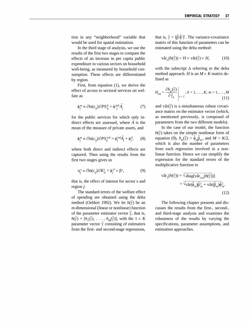
tion in any “neighborhood” variable that would be used for spatial estimation. In the third stage of analysis, we use the results of the first two stages to compare the effects of an increase in per capita public expenditure in various sectors on household well-being, as measured by household con-sumption. These effects are differentiated by region. First, from equation (1), we derive the effect of access to sectoral services on wel-fare as
fj* ≡ ∂ln(cij)/∂PSdij = find
j Aj (7)
for the public services for which only in-direct effects are assessed, where A is the mean of the measure of private assets, and
fj* ≡ ∂ln(cij)/∂PSijind = fj
indAj + fjd, (8)
where both direct and indirect effects are captured. Then using the results from the first two stages gives us
hjs ≡ ∂ln(cij)/∂Ks
jt = fjs* × bs, (9)
that is, the effect of interest for sector s and region j. The standard errors of the welfare effect of spending are obtained using the delta method (Oehlert 1992). We let h(g) be an m-dimensional (linear or nonlinear) function of the parameter estimator vector g, that is, h(g) = [h1(g), . . . , hM(g)], with the 1 × K parameter vector g consisting of estimators from the first- and second-stage regressions,
that is, g = [b′f′]′. The variance-covariance matrix of this function of parameters can be estimated using the delta method:
vârD(h(g)) = H × vâr(g) × H, (10)
with the subscript D referring to the delta method approach. H is an M × K matrix de- fined as
∂hm(g)Hmk = ———— |g = g
; k = 1, . . . , K; m = 1, . . . , M ∂gk
(11)
and vâr(g) is a simultaneous robust covari-ance matrix on the estimator vector (which, as mentioned previously, is composed of parameters from the two different models). In the case of our model, the function h(g) takes on the simple nonlinear form of equation (9), hm(g) = fmbm, and M = K/2, which is also the number of parameters from each regression involved in a non- linear function. Hence we can simplify the expression for the standard errors of the multiplicative function to
vârD(h(g)) = √````````````` diag[vârDm(h(g))]
= √````````````````` vâr(fm)b2m + vâr(bm)f2
m.
(12)
The following chapter presents and dis-cusses the results from the first-, second-, and third-stage analysis and examines the robustness of the results by varying the specifications, parameter assumptions, and estimation approaches.
EmPiRiCAl sTRATEgy 37

C H A P T E R 7
Estimation
First-Stage Analysis: Public Services, Private Assets, and Rural Welfare
T able 7.1 provides descriptive statistics on the variables included in the first-stage regression (also see the tables in Chapter 4), and Tables 7.2–7.8 give the estimation results from the first stage. Indicators of performance (access to services) are included
for the four sectors considered important for welfare enhancement in rural areas, namely ag-riculture, road infrastructure, education, and health. Table 7.2 presents the “short” model, in which the sector performance variables are intro-duced in terms of their direct and indirect effects, and their impact is not geographically dif-ferentiated, although region effects are included. Access to education (proxied by the primary school enrollment rate) and access to health care (measured by the distance to the nearest health facility) are interacted with the household’s labor assets, given that better access to educational and health services is expected to increase labor productivity. This model is also based on the hy-pothesis that higher average performance in agriculture and better access to roads will improve the contribution of farmers’ agricultural assets to their welfare. The variables indicating access to services and performance in four sectors are introduced as zonal-average variables, both to mitigate likely simultaneity when including household-specific variables on access to services in these sectors and also to enable, in the second-stage analysis, an examination of the link between public investments and these sector performance variables. The multistage nature of the empirical approach, and the concomitant choice of variables to proxy sectoral outcomes, implies an assumption for the education sector case worth mak-ing explicit. Using school enrollment rate as a proxy for access to education services within a locality assumes that there is relatively limited mobility of rural households over time, so that the average school access of a given individual’s current zonal residence is the relevant locality for this measure. This assumption is arguably not very stringent, given low levels of rural mobility (referring here to permanent resettlements rather than seasonal migration, which is common), and given the relatively large size of the geographic unit over which we aver-age the sector variables.1 We thus propose that the “temporal distance” between an education sector measure such as enrollment rate and the labor productivity of adult households can be bridged with a relatively plausible assumption of low household mobility in Ethiopia’s rural areas, while this measure is suitable for linking public expenditures to educational outcomes.
1In Ethiopia the zone is the second subnational administrative unit, below the region. The country has approxi-mately 60 zones.
38
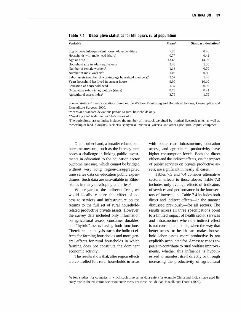
On the other hand, a broader educational outcome measure, such as the literacy rate, poses a challenge in linking public invest-ments in education to the education sector outcome measure, which cannot be bridged without very long region-disaggregated time series data on education public expen-ditures. Such data are unavailable in Ethio-pia, as in many developing countries.2
With regard to the indirect effects, we would ideally capture the effect of ac-cess to services and infrastructure on the returns to the full set of rural household-related productive private assets. However, the survey data included only information on agricultural assets, consumer durables, and “hybrid” assets having both functions. Therefore our analysis traces the indirect ef-fects for farming households and more gen-eral effects for rural households in which farming does not constitute the dominant economic activity. The results show that, after region effects are controlled for, rural households in areas
with better road infrastructure, education access, and agricultural productivity have higher consumption levels. Both the direct effects and the indirect effects, via the impact of public services on private productive as-sets, are significant in nearly all cases. Tables 7.3 and 7.4 consider alternative sectoral effects to those above. Table 7.3 includes only average effects of indicators of services and performance in the four sec-tors of interest, and Table 7.4 includes both direct and indirect effects—in the manner discussed previously—for all sectors. The results across all three specifications point to a limited impact of health sector services and infrastructure when the indirect effect is not considered, that is, when the way that better access to health care makes house-hold labor assets more productive is not explicitly accounted for. Access to roads ap- pears to contribute to rural welfare improve-ments, whether this influence is hypoth-esized to manifest itself directly or through increasing the productivity of agricultural
estimation 39
2A few studies, for countries in which such time series data exist (for example China and India), have used lit-eracy rate as the education sector outcome measure; these include Fan, Hazell, and Thorat (2000).
table 7.1 Descriptive statistics for ethiopia’s rural population
Variable Meana Standard deviationa
Log of per-adult-equivalent household expenditure 7.23 0.48Households with male head (share) 0.77 0.42Age of head 43.66 14.97Household size in adult-equivalents 3.43 1.35Number of female workersb 1.13 0.70Number of male workersb 1.03 0.80Labor assets (number of working-age household members)b 2.57 1.40Years household has lived in current house 9.00 10.10Education of household head 1.37 0.97Occupation solely in agriculture (share) 0.79 0.41Agricultural assets indexc 3.79 1.79
Source: Authors’ own calculations based on the Welfare Monitoring and Household Income, Consumption and Expenditure Surveys, 2000.aMeans and standard deviations pertain to rural households only.b“Working age” is defined as 14–50 years old.cThe agricultural assets index includes the number of livestock weighted by tropical livestock units, as well as ownership of land, plough(s), sickle(s), sprayer(s), tractor(s), yoke(s), and other agricultural capital equipment.

40 CHaPteR 7
table 7.2 indirect and direct countrywide rural welfare effects of public services and infrastructure access
Dependent variable: ln(household consumption per adult-equivalent)
Sector effects
Agriculture: indirect effects 0.00011 Yield × agricultural asset index (if farming household) (0.00010) Agriculture: direct effects 0.01498*** Yield (if nonfarming household) (0.00582) Road infrastructure: indirect effects 0.00185** Road density × agricultural asset index (0.00078) (if farming household) Road infrastructure: direct effects 0.01475* Road density (if nonfarming household) (0.00880) Education: indirect effects 0.06208*** Enrollment rate × labor assets (0.01389) Health: indirect effects –0.00110*** Distance to health facilities × labor assets (0.00042)
Region effects
Afar –0.27311*** (0.09123)Amhara –0.33167*** (0.03729)Beneshangul-Gumuz –0.46090*** (0.05251)Gambela –0.63596*** (0.07987)Oromia –0.24290*** (0.03538)SNNP –0.44841*** (0.03575)Somale 0.05327 (0.06148)Tigray –0.25212*** (0.04797)Constant 7.42702*** (0.07904)
Notes: Ordinary least squares estimation with robust standard errors; errors corrected for enumeration area cluster effects. Standard errors in parentheses. Coefficients are significant at the * 10 percent, ** 5 percent, and *** 1 percent levels, respectively. Variables used for access to services and performance in four sectors—agriculture: crop yield (average physical yield of all annual crops, in quintals per hectare); road infrastructure: road density (kilometers of roads per 1,000 persons); education: primary enrollment rate – gross enrollment rate in primary school (grades 1–8); health: access to health facilities – distance to nearest health facility (in kilometers). Road infrastructure, education, health, and agriculture variables are measured as zonal averages. SNNP—Southern Nations, Nationalities, and Peoples.
Household characteristics
Head is male –0.00962 (0.01615)Age of head –0.00178 (0.00231) Age of head squared 0.00002 (0.00002)Household size (adult-equivalents) –0.09741*** (0.00888)Number of years lived here 0.00068 (0.00079)Number of female workers –0.01240 (0.01151)Number of male workers –0.00480 (0.01108)Education of head 0.11569*** (0.00755)Engaged in agriculture 0.24345*** (0.06662)
Number of observations 7,871Number of clusters 674F-statistic (23,673) 42.05***R2 0.19

estimation 41
assets. On the other hand, the contribution to rural welfare of performance in the agri-cultural sector appears to be more strongly captured directly. The contribution of access to education services to welfare is positive and significant when either only average direct effects or only indirect effects are considered.
The region effects include all regions but the three city-states Addis Ababa, Dire Dawa, and Harari, which are predominantly urban. Predictably, living in virtually any of the predominantly rural regions is associated with lower welfare compared to residence in the rural areas within one of the three city-states. Not surprisingly, given the sub-
table 7.3 average countrywide rural welfare effects of public services and infrastructure access
Dependent variable: ln(household consumption per adult-equivalent)
Sector effects
Agriculture: average effects 0.020177*** (0.00502) Road infrastructure: average effects 0.066524** (0.03318) Education: average effects 0.395526*** (0.07484) Health: average effects –0.001990 (0.00148)
Region effects
Afar –0.243317*** (0.08066)Amhara –0.261932*** (0.04303)Beneshangul-Gumuz –0.655155*** (0.09435)Gambela –1.594032*** (0.39920)Oromia –0.247577*** (0.04153)SNNP –0.461964*** (0.04160)Somale 0.220302*** (0.07434)Tigray –0.260067*** (0.04857)Constant 7.057753*** (0.09503)
Notes: Ordinary least squares estimation with robust standard errors; errors corrected for enumeration area cluster effects. Standard errors in parentheses. Coefficients are significant at the * 10 percent, ** 5 percent, and *** 1 percent levels, respectively. Variables used for access to services and performance in four sectors—agriculture: crop yield (average physical yield of all annual crops, in quintals per hectare); road infrastructure: road density (kilometers of roads per 1,000 persons); education: primary enrollment rate – gross enrollment rate in primary school (grades 1–8); health: access to health facilities – distance to nearest health facility (in kilometers). Road infrastructure, education, health, and agriculture variables are measured as zonal averages. SNNP—Southern Nations, Nationalities, and Peoples.a“Working age” is defined as 14–50 years old.
Household characteristics
Head is male –0.002535 (0.01546)Age of head –0.000617 (0.00228)Age of head squared 0.000004 (0.00002)Household size –0.080022*** (adult-equivalents) (0.00730)Number of years lived here 0.001366* (0.00072)Number of female workersa 0.007249 (0.00923)Number of male workersa 0.015767* (0.00895)Education of head 0.111982*** (0.00751)Engaged in agriculture 0.067010*** (0.01620)
Number of observations 7,871Number of clusters 674F-statistic (21,673) 43.77***R2 0.20
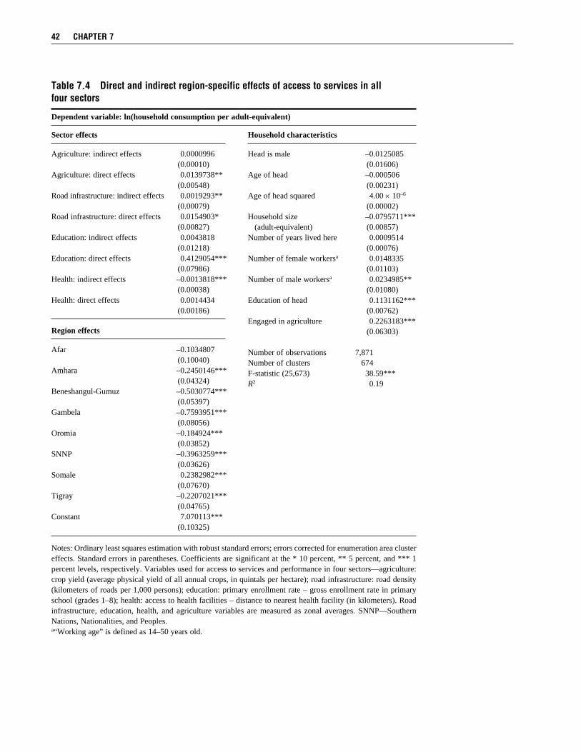
42 CHaPteR 7
table 7.4 Direct and indirect region-specific effects of access to services in all four sectors
Dependent variable: ln(household consumption per adult-equivalent)
Sector effects
Agriculture: indirect effects 0.0000996 (0.00010) Agriculture: direct effects 0.0139738** (0.00548) Road infrastructure: indirect effects 0.0019293** (0.00079) Road infrastructure: direct effects 0.0154903* (0.00827) Education: indirect effects 0.0043818 (0.01218) Education: direct effects 0.4129054*** (0.07986) Health: indirect effects –0.0013818*** (0.00038) Health: direct effects 0.0014434 (0.00186)
Region effects
Afar –0.1034807 (0.10040)Amhara –0.2450146*** (0.04324)Beneshangul-Gumuz –0.5030774*** (0.05397)Gambela –0.7593951*** (0.08056)Oromia –0.184924*** (0.03852)SNNP –0.3963259*** (0.03626)Somale 0.2382982*** (0.07670)Tigray –0.2207021*** (0.04765)Constant 7.070113*** (0.10325)
Notes: Ordinary least squares estimation with robust standard errors; errors corrected for enumeration area cluster effects. Standard errors in parentheses. Coefficients are significant at the * 10 percent, ** 5 percent, and *** 1 percent levels, respectively. Variables used for access to services and performance in four sectors—agriculture: crop yield (average physical yield of all annual crops, in quintals per hectare); road infrastructure: road density (kilometers of roads per 1,000 persons); education: primary enrollment rate – gross enrollment rate in primary school (grades 1–8); health: access to health facilities – distance to nearest health facility (in kilometers). Road infrastructure, education, health, and agriculture variables are measured as zonal averages. SNNP—Southern Nations, Nationalities, and Peoples.a“Working age” is defined as 14–50 years old.
Household characteristics
Head is male –0.0125085 (0.01606)Age of head –0.000506 (0.00231)Age of head squared 4.00 × 10⁻⁶
(0.00002)Household size –0.0795711*** (adult-equivalent) (0.00857)Number of years lived here 0.0009514 (0.00076)Number of female workersa 0.0148335 (0.01103)Number of male workersa 0.0234985** (0.01080)Education of head 0.1131162*** (0.00762)Engaged in agriculture 0.2263183*** (0.06303)
Number of observations 7,871Number of clusters 674F-statistic (25,673) 38.59***R2 0.19

stantial interregional economic differences in Ethiopia, the region effects are strong in explaining rural welfare. Their magnitudes also follow quite closely the information on regional poverty in Table 3.2: Rural resi-dents of Beneshangul-Gumuz and Gambela, the two poorest regions, also have the low-est expenditure levels. In contrast Somale, which has the lowest poverty rate, is associ-ated with the highest levels of household expenditure (however, the Somale effect is not statistically significant). As is commonly found, here too larger households are associated with lower wel-fare, even when accounting for economies of scale, as does the measure of household size. Equally commonly, households with more highly educated heads enjoy greater material welfare. Occupation plays an inter-esting role for welfare: within rural areas, it is those households predominantly engaged in farming that fare better, compared to those who reside in the rural areas and yet are engaged in other economic activities. This may point to the lack of vibrant non-farm opportunities in rural Ethiopia. A common thread across the estima-tions so far is that the region effects play an important role in explaining rural incomes. This is intuitive in light of the very strong regional variations in welfare in Ethiopia. But the strongly significant estimates of the region effects in Tables 7.2–7.4 also raise the question of whether our central results are sensitive to dominant observations asso-ciated with any given region. Expressed dif-ferently, it may be not only that region ef-fects are important as parameter shifters but also that the role of sectoral performance for rural incomes may be to a great extent driven by one region, so that if we were to exclude all observations of one influential region from the analysis, our results on the impact of sectoral variables on incomes would change in a meaningful way. Table 7.5 indicates the extent of robust-ness of the results of the short model to the exclusion of observations associated with any single region. The first column
reproduces Table 7.2, and the subsequent columns estimate the same model after ex-cluding all observations associated with one region. The flagged coefficients indicate nontrivial changes from the base model: either there was a change in the direction of influence—a significant coefficient changed signs—or a change in signifi-cance—a significant coefficient became nonsignificant or vice versa. In the short model, conclusions on access to roads are the least robust to variations in the obser-vation set. The significance of the average (across all regions) effect of access to roads on rural incomes becomes nonsignificant when any one of six regions is excluded from the dataset. Exclusion of the Afar re-gion has the most influential effect, not only on coefficient significance but also on coef-ficient magnitude and type of effect (both direct and indirect effects become small and insignificant). As will be seen later in the region-differentiated analysis, Afar is also one of the regions in which returns to road expenditure are large and significant. Using the formulation in Table 7.2 as the main specification of the impact of ac-cess to public services and infrastructure in the four sectors, we expand this specifica-tion to capture how the role of access to services for household welfare may be re-gionally differentiated (Table 7.6). Results of this main specification will, analogous to the short models discussed previously, also be compared against a case in which regionally differentiated effects are only assessed in the average, that is, they are not parsed into direct and indirect effects. This is presented in Table 7.7. The results of the regionally differenti-ated first-stage estimation are presented in three columns in Table 7.6 to allow for compact presentation, but they refer to a single regression. The same goes for Table 7.7. These results serve primarily as an input to the third-stage analysis and are therefore mainly interpreted as part of our discussion of that stage. However, a few interesting ob-servations can already be made at this stage.
estimation 43

tabl
e 7.
5 R
obus
tnes
s of
sho
rt fir
st-s
tage
mod
el to
exc
lusi
on o
f obs
erva
tions
Dep
ende
nt v
aria
ble:
ln(h
ouse
hold
con
sum
ptio
n pe
r ad
ult-
equi
vale
nt)
Ben
esha
ngul
-E
xclu
ded
obse
rvat
ions
N
one
Afa
r A
mha
ra
Gum
uz
Gam
bela
O
rom
ia
Som
ale
SNN
P
Tig
ray
Sect
or e
ffec
tsA
gric
ultu
re: i
ndir
ect e
ffec
ts
0.00
011
0.00
04
0.00
009
0.00
01
0.00
005
0.00
017
0.00
011
0.00
001
0.00
009
(0
.000
10)
(0.0
003)
(0
.000
1)
(0.0
001)
(0
.000
1)
(0.0
001)
(0
.000
1)
(0.0
001)
(0
.000
1)A
gric
ultu
re: d
irec
t eff
ects
0.
0149
8***
0.
0144
2**
0.01
998*
**
0.01
54**
* 0.
0191
8***
0.
0148
2**
0.01
49**
0.
0050
8 0.
0154
7***
(0
.005
82)
(0.0
064)
(0
.006
1)
(0.0
059)
(0
.005
8)
(0.0
072)
(0
.006
1)
(0.0
062)
(0
.005
8)R
oad
infr
astr
uctu
re: i
ndir
ect e
ffec
ts
0.00
185*
* 0.
0001
6+
0.00
177*
* 0.
0015
2**
0.00
444*
**
0.00
17**
0.
0018
3**
0.00
257*
* 0.
0018
**
(0.0
0078
) (0
.000
7)
(0.0
007)
(0
.000
7)
(0.0
017)
(0
.000
8)
(0.0
008)
(0
.001
) (0
.000
8)R
oad
infr
astr
uctu
re: d
irec
t eff
ects
0.
0147
5*
0.00
263+
0.
0103
5+
0.00
974+
0.
1056
5***
0.
0122
5+
0.01
421+
0.
0247
8***
0.
0138
9+
(0.0
0880
) (0
.008
5)
(0.0
086)
(0
.008
8)
(0.0
238)
(0
.009
6)
(0.0
088)
(0
.009
1)
(0.0
088)
Edu
catio
n: in
dire
ct e
ffec
ts
0.06
208*
**
0.05
959*
**
0.06
402*
**
0.06
174*
**
0.07
902*
**
0.06
9***
0.
0610
3***
0.
0345
**
0.06
252*
**
(0.0
1389
) (0
.015
2)
(0.0
147)
(0
.016
) (0
.014
2)
(0.0
149)
(0
.014
3)
(0.0
135)
(0
.014
1)H
ealth
: ind
irec
t eff
ects
–0
.001
10**
* 0.
0003
4 –0
.001
23**
* –0
.001
16**
–0
.001
02**
* –0
.001
41**
* –0
.001
13**
* –0
.001
22**
* –0
.001
14**
*
(0.0
0042
) (0
.000
4)
(0.0
004)
(0
.000
5)
(0.0
004)
(0
.000
4)
(0.0
004)
(0
.000
4)
(0.0
004)
Hou
seho
ld c
hara
cter
isti
csH
ead
is m
ale
–0.0
0962
0.
0024
4 –0
.022
66
–0.0
069
–0.0
0984
–0
.019
–0
.014
02
0.00
948
–0.0
1115
(0
.016
15)
(0.0
157)
(0
.017
8)
(0.0
169)
(0
.016
2)
(0.0
187)
(0
.016
4)
(0.0
185)
(0
.017
4)A
ge o
f he
ad
–0.0
0178
–0
.000
07
–0.0
0488
+*
–0.0
0089
–0
.001
97
–0.0
0337
–0
.001
39
–0.0
007
–0.0
0171
(0
.002
31)
(0.0
022)
(0
.002
5)
(0.0
024)
(0
.002
3)
(0.0
028)
(0
.002
4)
(0.0
026)
(0
.002
4)A
ge o
f he
ad s
quar
ed
0.00
002
0.00
0004
0.
0000
51+
**
0.00
0009
0.
0000
22
0.00
0039
0.
0000
16
0.00
0003
0.
0000
18
(0.0
0002
) (0
.000
02)
(0.0
0003
) (0
.000
02)
(0.0
0002
) (0
.000
03)
(0.0
0002
) (0
.000
03)
(0.0
0002
)
44 CHaPteR 7

Hou
seho
ld s
ize
(adu
lt-eq
uiva
lent
s)
–0.0
9741
***
–0.1
0845
***
–0.1
0342
***
–0.0
9881
***
–0.1
0123
***
–0.1
0022
***
–0.0
9235
***
–0.0
8824
***
–0.0
9416
***
(0
.008
88)
(0.0
094)
(0
.009
7)
(0.0
093)
(0
.008
8)
(0.0
102)
(0
.009
2)
(0.0
099)
(0
.009
1)N
umbe
r of
yea
rs li
ved
here
0.
0006
8 0.
0009
8 0.
0006
3 0.
0007
3 0.
0008
1 0.
0003
6 0.
0004
8 0.
0020
7***
–0
.000
34
(0.0
0079
) (0
.000
8)
(0.0
009)
(0
.000
8)
(0.0
008)
(0
.000
9)
(0.0
008)
(0
.000
8)
(0.0
009)
Num
ber
of f
emal
e w
orke
rs
–0.0
1240
–0
.023
07+
**
–0.0
0834
–0
.013
02
–0.0
1964
+*
–0.0
0726
–0
.015
29
0.00
124
–0.0
1386
(0
.011
51)
(0.0
117)
(0
.012
3)
(0.0
125)
(0
.011
5)
(0.0
13)
(0.0
119)
(0
.013
) (0
.011
7)N
umbe
r of
mal
e w
orke
rs
–0.0
0480
–0
.008
68
–0.0
0758
0.
0000
1 –0
.010
65
–0.0
1598
–0
.008
44
0.01
83
–0.0
0524
(0
.011
08)
(0.0
117)
(0
.012
4)
(0.0
116)
(0
.011
2)
(0.0
12)
(0.0
114)
(0
.012
1)
(0.0
115)
Edu
catio
n of
hea
d 0.
1156
9***
0.
1181
2***
0.
1079
9***
0.
1122
6***
0.
1164
1***
0.
1294
***
0.11
534*
**
0.10
612*
**
0.11
594*
**
(0.0
0755
) (0
.007
5)
(0.0
069)
(0
.008
) (0
.007
9)
(0.0
088)
(0
.007
7)
(0.0
099)
(0
.007
6)E
ngag
ed in
agr
icul
ture
0.
2434
5***
0.
2105
***
0.30
169*
**
0.24
924*
**
0.34
022*
**
0.23
751*
**
0.24
59**
* 0.
1373
8**
0.24
974*
**
(0.0
6662
) (0
.073
5)
(0.0
725)
(0
.067
7)
(0.0
694)
(0
.076
5)
(0.0
703)
(0
.067
8)
(0.0
676)
Con
stan
t 7.
4270
2***
7.
4344
4***
7.
4796
3***
7.
4096
9***
7.
3239
5***
7.
4540
2***
7.
4137
7***
7.
4924
3***
7.
4215
8***
(0
.079
04)
(0.0
842)
(0
.085
9)
(0.0
805)
(0
.080
5)
(0.0
91)
(0.0
816)
(0
.083
5)
(0.0
807)
Reg
ion
effe
cts
incl
uded
Y
es
Yes
Y
es
Yes
Y
es
Yes
Y
es
Yes
Y
esN
umbe
r of
obs
erva
tions
7,
871
7,51
4 6,
184
7,37
0 7,
661
6,10
5 7,
616
6,03
2 7,
321
Num
ber
of c
lust
ers
7,67
4 7,
641
7,53
0 7,
631
7,65
6 7,
523
7,65
2 7,
518
7,62
7F-
stat
istic
42
.05*
**
43.7
3***
42
.73*
**
42.8
1***
42
.19*
**
37.3
4***
40
.79
29.1
1***
42
.16*
**R
2 0.
19
0.20
0.
21
0.19
0.
20
0.21
0.
17
0.17
0.
19
Not
es: O
rdin
ary
leas
t squ
ares
est
imat
ion
with
rob
ust s
tand
ard
erro
rs; e
rror
s co
rrec
ted
for
enum
erat
ion
area
clu
ster
eff
ects
. Sta
ndar
d er
rors
in p
aren
thes
es. C
oeff
icie
nts
are
sign
ific
ant a
t the
* 1
0 pe
rcen
t, **
5 p
erce
nt, a
nd *
** 1
per
cent
leve
ls, r
espe
ctiv
ely.
Var
iabl
es u
sed
for
acce
ss to
ser
vice
s an
d pe
rfor
man
ce in
fou
r se
ctor
s—ag
ricu
lture
: cro
p yi
eld
(ave
rage
phy
sica
l yie
ld o
f al
l ann
ual c
rops
, in
quin
tals
pe
r he
ctar
e); r
oad
infr
astr
uctu
re: r
oad
dens
ity (
kilo
met
ers
of r
oads
per
1,0
00 p
erso
ns);
edu
catio
n: p
rim
ary
enro
llmen
t rat
e –
gros
s en
rollm
ent r
ate
in p
rim
ary
scho
ol (
grad
es 1
–8);
hea
lth: a
cces
s to
hea
lth
faci
litie
s –
dist
ance
to
near
est
heal
th f
acili
ty (
in k
ilom
eter
s). R
oad
infr
astr
uctu
re, e
duca
tion,
hea
lth, a
nd a
gric
ultu
re v
aria
bles
are
mea
sure
d as
zon
al a
vera
ges.
SN
NP—
Sout
hern
Nat
ions
, Nat
iona
litie
s,
and
Peop
les.
+ d
enot
es n
ontr
ivia
l cha
nges
fro
m th
e ba
se m
odel
.
estimation 45
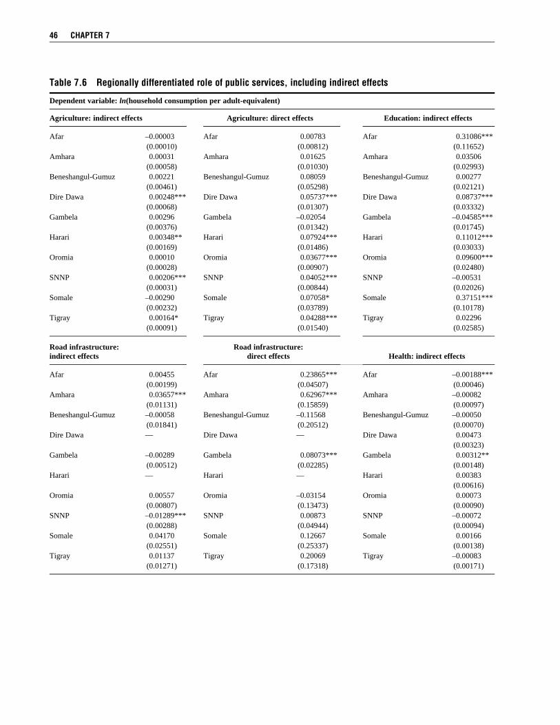
46 CHaPteR 7
table 7.6 Regionally differentiated role of public services, including indirect effects
Dependent variable: ln(household consumption per adult-equivalent)
Agriculture: indirect effects Agriculture: direct effects Education: indirect effects
Afar –0.00003 Afar 0.00783 Afar 0.31086*** (0.00010) (0.00812) (0.11652)Amhara 0.00031 Amhara 0.01625 Amhara 0.03506 (0.00058) (0.01030) (0.02993)Beneshangul-Gumuz 0.00221 Beneshangul-Gumuz 0.08059 Beneshangul-Gumuz 0.00277 (0.00461) (0.05298) (0.02121)Dire Dawa 0.00248*** Dire Dawa 0.05737*** Dire Dawa 0.08737*** (0.00068) (0.01307) (0.03332)Gambela 0.00296 Gambela –0.02054 Gambela –0.04585*** (0.00376) (0.01342) (0.01745)Harari 0.00348** Harari 0.07924*** Harari 0.11012*** (0.00169) (0.01486) (0.03033)Oromia 0.00010 Oromia 0.03677*** Oromia 0.09600*** (0.00028) (0.00907) (0.02480)SNNP 0.00206*** SNNP 0.04052*** SNNP –0.00531 (0.00031) (0.00844) (0.02026)Somale –0.00290 Somale 0.07058* Somale 0.37151*** (0.00232) (0.03789) (0.10178)Tigray 0.00164* Tigray 0.04288*** Tigray 0.02296 (0.00091) (0.01540) (0.02585)
Road infrastructure: Road infrastructure: indirect effects direct effects Health: indirect effects
Afar 0.00455 Afar 0.23865*** Afar –0.00188*** (0.00199) (0.04507) (0.00046)Amhara 0.03657*** Amhara 0.62967*** Amhara –0.00082 (0.01131) (0.15859) (0.00097)Beneshangul-Gumuz –0.00058 Beneshangul-Gumuz –0.11568 Beneshangul-Gumuz –0.00050 (0.01841) (0.20512) (0.00070)Dire Dawa — Dire Dawa — Dire Dawa 0.00473 (0.00323)Gambela –0.00289 Gambela 0.08073*** Gambela 0.00312** (0.00512) (0.02285) (0.00148)Harari — Harari — Harari 0.00383 (0.00616)Oromia 0.00557 Oromia –0.03154 Oromia 0.00073 (0.00807) (0.13473) (0.00090)SNNP –0.01289*** SNNP 0.00873 SNNP –0.00072 (0.00288) (0.04944) (0.00094)Somale 0.04170 Somale 0.12667 Somale 0.00166 (0.02551) (0.25337) (0.00138)Tigray 0.01137 Tigray 0.20069 Tigray –0.00083 (0.01271) (0.17318) (0.00171)

A strong interregional variation is seen in the effects of road access. This effect is strong and significant in two neighboring regions (Afar and Amhara) in both specifi-cations of Table 7.6 and Table 7.7. These regions are agroecologically quite different, with Afar being a predominantly pastoral re-gion and Amhara consisting of mostly seden-tary and partly agropastoral households. The impact of road density is also positive and significant in Gambela in the main regression (Table 7.6). As noted earlier (Tables 4.4 and 4.5), Afar and Gambela have relatively high road densities, even though they are often referred to as backward regions. Amhara’s road density is medium to high compared to that in other regions. On the other hand, zonal-average road density has a significant and the lowest ef-fect on the contribution of rural households’ agricultural assets to their income. This suggests an interesting analogue between
the results for this region and those for the regions described previously, which were found to have high welfare returns to access to roads. As shown in Table 4.4, SNNP had the poorest access to roads in all the years for which data are available. This, com-bined with the generally positive relation-ship between levels of and returns to road density that was identified when results for the other regions were examined, suggests that access to all-weather roads may yield increasing returns in terms of gains to the productivity of private household assets. The specification also allows examina-tion of whether household consumption increases when average agricultural perfor-mance is high. This effect may be realized directly and, among those whose main livelihood is farming, indirectly by generat-ing higher returns to their agricultural as-sets. Unlike the case of road infrastructure, the effects across regions are less varied
estimation 47
table 7.6 Continued
Household characteristics
Head is male –0.01072 Number of female workersa –0.01119 (0.01526) (0.01199) Age of head –0.00165 Number of male workersa –0.00402 (0.00222) (0.01135) Age of head squared 0.00002 Education of head 0.11385*** (0.00002) (0.00799) Household size –0.10350*** Engaged in agriculture 0.47809*** (adult-equivalents) (0.00911) (0.11134) Number of years lived here 0.00055 Constant 6.83598*** (0.00073) (0.11391) Number of observations 7,871 Number of clusters 674 F-statistic (65,673) 22.38*** R2 0.22
Notes: Ordinary least squares estimation with robust standard errors; errors corrected for enumeration area cluster effects. Standard errors in parentheses. Coefficients are significant at the * 10 percent, ** 5 percent, and *** 1 percent levels, respectively. Variables used for access to services and performance in four sectors—agriculture: crop yield (average physical yield of all annual crops, in quintals per hectare); road in-frastructure: road density (kilometers of roads per 1,000 persons); education: primary enrollment rate – gross enrollment rate in primary school (grades 1–8); health: access to health facilities – distance to nearest health facility (in kilometers). Road infrastructure, education, health, and agriculture variables are measured as zonal averages. — indicates that an estimate of the coefficient could not be derived due to collinearity. SNNP—Southern Nations, Nationalities, and Peoples.a”Working age” is defined as 14–50 years old.
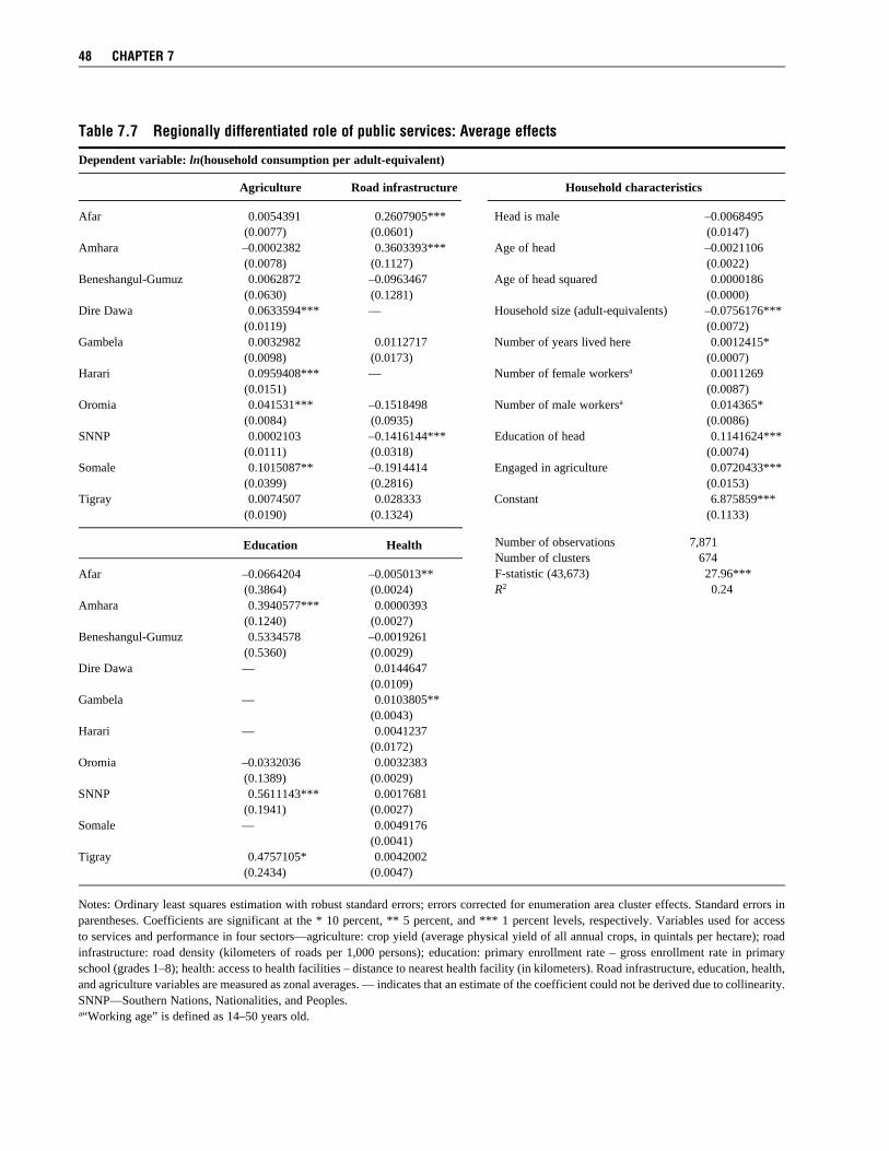
48 CHaPteR 7
table 7.7 Regionally differentiated role of public services: average effects
Dependent variable: ln(household consumption per adult-equivalent)
Agriculture Road infrastructure Household characteristics
Afar 0.0054391 0.2607905*** Head is male –0.0068495 (0.0077) (0.0601) (0.0147)Amhara –0.0002382 0.3603393*** Age of head –0.0021106 (0.0078) (0.1127) (0.0022)Beneshangul-Gumuz 0.0062872 –0.0963467 Age of head squared 0.0000186 (0.0630) (0.1281) (0.0000)Dire Dawa 0.0633594*** — Household size (adult-equivalents) –0.0756176*** (0.0119) (0.0072)Gambela 0.0032982 0.0112717 Number of years lived here 0.0012415* (0.0098) (0.0173) (0.0007)Harari 0.0959408*** — Number of female workersa 0.0011269 (0.0151) (0.0087)Oromia 0.041531*** –0.1518498 Number of male workersa 0.014365* (0.0084) (0.0935) (0.0086)SNNP 0.0002103 –0.1416144*** Education of head 0.1141624*** (0.0111) (0.0318) (0.0074)Somale 0.1015087** –0.1914414 Engaged in agriculture 0.0720433*** (0.0399) (0.2816) (0.0153)Tigray 0.0074507 0.028333 Constant 6.875859*** (0.0190) (0.1324) (0.1133)
Education Health
Afar –0.0664204 –0.005013** (0.3864) (0.0024)Amhara 0.3940577*** 0.0000393 (0.1240) (0.0027)Beneshangul-Gumuz 0.5334578 –0.0019261 (0.5360) (0.0029)Dire Dawa — 0.0144647 (0.0109)Gambela — 0.0103805** (0.0043)Harari — 0.0041237 (0.0172)Oromia –0.0332036 0.0032383 (0.1389) (0.0029)SNNP 0.5611143*** 0.0017681 (0.1941) (0.0027)Somale — 0.0049176 (0.0041)Tigray 0.4757105* 0.0042002 (0.2434) (0.0047)
Notes: Ordinary least squares estimation with robust standard errors; errors corrected for enumeration area cluster effects. Standard errors in parentheses. Coefficients are significant at the * 10 percent, ** 5 percent, and *** 1 percent levels, respectively. Variables used for access to services and performance in four sectors—agriculture: crop yield (average physical yield of all annual crops, in quintals per hectare); road infrastructure: road density (kilometers of roads per 1,000 persons); education: primary enrollment rate – gross enrollment rate in primary school (grades 1–8); health: access to health facilities – distance to nearest health facility (in kilometers). Road infrastructure, education, health, and agriculture variables are measured as zonal averages. — indicates that an estimate of the coefficient could not be derived due to collinearity. SNNP—Southern Nations, Nationalities, and Peoples.a“Working age” is defined as 14–50 years old.
Number of observations 7,871Number of clusters 674F-statistic (43,673) 27.96***R2 0.24
and are significant for a greater number of regions. Zonal-average agricultural per-formance shows the strongest effects on households—and the welfare returns to their productive assets—in Dire Dawa and Harari. Given that the cities of Dire Dawa and Harer respectively dominate these two regions, this may suggest that the proximity of rural households to major markets con-siderably increases the income returns from stronger agricultural performance. Interestingly access to education shows the highest returns to labor assets in the Afar and Somale regions, which also have the lowest enrollment ratios (Table 4.10). Returns to education investment are lowest in Gambela, which has among the highest enrollment. In contrast to the apparently positive relationship between levels and impact seen in the road infrastructure sec-tor, it appears here that access to education leverages household labor assets to a greater degree in regions where the levels of access are lowest, and vice versa. While Tables 7.2–7.4 showed that re-ducing the distance to health facilities had a significant positive average effect on rural welfare, specifically through making labor more productive, we see in Tables 7.6 and 7.7 that this effect is weak and largely insignificant when disaggregating the effect by region. Only in Afar is a reduction of distance to health facilities associated with greater rural consumption, and the effect is negative in Gambela. The fact that the coefficients for the SNNP and Gambela regions related to road access and access to social services, respec-tively, are not only low but negative serves in a sense as a reminder that this is only a partial analysis of the benefits that may derive from public services. While road in-frastructure, for example, may serve rural and urban residents alike, we are only con-sidering the effects on rural households’ incomes. Furthermore the intended goals of and the actual gains from the provi-sion of these services may be primarily in the form of other outcomes, for example
improving equitable access to services, ad-dressing extreme poverty, and ensuring so-cial stability. This report, however, focuses only on rural household incomes (proxied by household expenditure). If the improve-ment of sectoral performance to meet one set of goals comes at the expense of other goals, then such partial analysis will not be able to uncover the full social benefits of service provision, and—as may be the case in this study—may only highlight negative effects, if any. In the estimation, the inclusion of zonal-average sector indicators as potential de-terminants of household welfare—in order to mitigate the simultaneity that is nearly sure to arise if one were to instead include household-level access to services—means that, on the downside, one may not be able to capture the heterogeneous provi-sion of, and access to, services within the geographic area. For example, if zones in SNNP with better road networks also hap-pen to be concentrated more in urban areas within the zone than in poor-network zones, then a partial focus on the effect of road density on rural welfare may present the type of result we found previously. We cannot say conclusively whether these dynamics are in play in the case of SNNP, especially given that the nonfarm economy in that region is still heavily under- developed. This may suggest the need for additional work, including explicit model-ing of additional mechanisms (other than returns to agricultural assets) by which road infrastructure may affect household income and consideration of the range of potential outcomes (beyond rural income) that may obtain from improvements in sector-specific performance indicators. Finally, Table 7.8 presents a robust-ness analysis on the primary long model (Table 7.6) analogous to the one discussed with respect to the short model (Table 7.5). Here again we subject the model to data sensitivity analysis by estimating the model after exclusion of all observations associated with one region at a time. Unlike
estimation 49

50 CHaPteR 7
tabl
e 7.
8 R
obus
tnes
s of
prim
ary
first
-sta
ge m
odel
to e
xclu
sion
of o
bser
vatio
ns
Exc
lude
d
B
enes
hang
ul-
obse
rvat
ions
N
one
Afa
r A
mha
ra
Gum
uz
Dir
e D
awa
Gam
bela
H
arar
i O
rom
ia
SNN
P
Som
ale
Tig
ray
Agr
icul
ture
: in
dire
ct e
ffec
tsA
far
–0.0
0002
99
—
–0.0
0005
45
–0.0
0004
33
–0.0
0002
32
–0.0
0002
75
–0.0
0002
04
0.00
0014
6 –0
.000
0809
–0
.000
0179
–0
.000
0264
Am
hara
0.
0003
11
0.00
0379
—
0.
0002
23
0.00
0365
6 0.
0003
267
0.00
0379
5 0.
0006
119
0.00
0021
6 0.
0003
971
0.00
0305
8B
enes
hang
ul-G
umuz
0.
0022
125
0.00
2229
5 0.
0012
85
—
0.00
2501
8 0.
0022
954
0.00
2524
5 0.
0033
459
0.00
1185
4 0.
0025
64
0.00
2280
2D
ire
Daw
a 0.
0024
799*
**
0.00
2489
1***
0.
0023
021*
**
0.00
2402
9***
—
0.
0024
962*
**
0.00
2545
5***
0.
0026
897*
**
0.00
2279
7***
0.
0025
528*
**
0.00
2485
***
Gam
bela
0.
0029
576
0.00
2877
6 0.
0025
237
0.00
2737
1 0.
0031
325
—
0.00
3118
3 0.
0034
247
0.00
2722
5 0.
0031
054
0.00
2906
2H
arar
i 0.
0034
789*
* 0.
0034
89**
0.
0032
166*
* 0.
0033
617*
* 0.
0035
693*
* 0.
0034
976*
* —
0.
0038
093*
* 0.
0031
723*
* 0.
0035
835*
* 0.
0034
824*
*O
rom
ia
0.00
0102
5 0.
0000
965
0.00
0118
8 0.
0001
072
0.00
0098
8 0.
0001
026
0.00
0096
5 —
0.
0001
157
0.00
0098
2 0.
0001
053
SNN
P 0.
0020
613*
**
0.00
2061
8***
0.
0019
316*
**
0.00
2017
7***
0.
0021
048*
**
0.00
2068
1***
0.
0021
051*
**
0.00
2176
***
—
0.00
2104
3***
0.
0020
886*
**So
mal
e –0
.002
8985
–0
.003
0259
–0
.002
8135
–0
.002
8398
–0
.002
9095
–0
.002
9104
–0
.002
923
–0.0
0314
48
–0.0
0252
45
—
–0.0
0288
16T
igra
y 0.
0016
399*
0.
0016
847*
0.
0014
028
0.00
1533
* 0.
0017
111*
0.
0016
602*
0.
0017
172*
0.
0019
743*
* 0.
0012
658+
0.
0017
456*
—
Agr
icul
ture
: di
rect
eff
ects
Afa
r 0.
0078
255
—
0.01
1015
3 0.
0066
725
0.00
7805
0.
0078
849
0.00
8086
9 0.
0087
928
0.00
5065
2 0.
0080
678
0.00
8628
2A
mha
ra
0.01
6251
0.
0116
073
—
0.01
4979
6 0.
0163
485
0.01
6290
8 0.
0164
266
0.01
702
0.01
3914
4 0.
0165
19
0.01
7110
1*B
enes
hang
ul-G
umuz
0.
0805
927
0.07
0625
7 0.
0895
578*
—
0.
0817
426
0.08
0669
8 0.
0812
551
0.07
8942
3 0.
0780
958
0.08
1737
6 0.
0807
677
Dir
e D
awa
0.05
7368
2***
0.
0498
077*
**
0.06
4378
***
0.05
5922
5***
—
0.
0573
563*
**
0.05
7170
7***
0.
0563
834*
**
0.05
5924
***
0.05
7246
2***
0.
0584
25**
*G
ambe
la
–0.0
2053
8 –0
.022
0228
+*
–0.0
2052
52
–0.0
2121
17
–0.0
2000
64
—
–0.0
2016
37
–0.0
2012
3 –0
.021
2617
–0
.020
0157
–0
.020
3199
Har
ari
0.07
9236
4***
0.
0705
573*
**
0.08
6677
3***
0.
0776
32**
* 0.
0789
88**
* 0.
0792
132*
**
—
0.07
8199
***
0.07
7907
6***
0.
0790
12**
* 0.
0805
289*
**O
rom
ia
0.03
6767
8***
0.
0314
319*
**
0.04
1881
2***
0.
0357
577*
**
0.03
6559
8***
0.
0367
82**
* 0.
0365
667*
**
—
0.03
5513
2***
0.
0366
574*
**
0.03
7595
9***
SNN
P 0.
0405
188*
**
0.03
5418
7***
0.
0449
179*
**
0.03
9721
2***
0.
0403
207*
**
0.04
0493
***
0.04
0467
8***
0.
0396
876*
**
—
0.04
0371
9***
0.
0414
594*
**So
mal
e 0.
0705
771*
0.
0510
453
0.09
0131
6**
0.06
9428
1*
0.06
8428
9*
0.07
0268
2*
0.06
8324
8*
0.06
0420
2 0.
0791
286*
—
0.
0731
651*
Tig
ray
0.04
2884
7***
0.
0363
937*
* 0.
0477
338*
**
0.04
1608
3***
0.
0428
567*
**
0.04
2958
4***
0.
0429
573*
**
0.04
274*
* 0.
0394
679*
* 0.
0432
826*
**
—
Roa
d in
fras
truc
ture
: in
dire
ct e
ffec
tsA
far
0.00
4546
5**
—
0.00
4463
7**
0.00
4572
**
0.00
4542
4**
0.00
4542
4**
0.00
4532
6**
0.00
4511
**
0.00
4637
5**
0.00
4546
9**
0.00
4480
5**
Am
hara
0.
0365
7***
0.
0362
494*
**
—
0.03
5457
3***
0.
0376
011*
**
0.03
6860
3***
0.
0376
635*
**
0.03
9993
5***
0.
0326
377*
**
0.03
7809
5***
0.
0377
507*
**B
enes
hang
ul-G
umuz
–0
.000
5838
–0
.000
5169
0.
0024
839
—
–0.0
0154
07
–0.0
0087
32
–0.0
0160
54
–0.0
0422
65
0.00
2685
–0
.001
7264
–0
.000
8875
Gam
bela
–0
.002
8907
–0
.002
7779
–0
.002
3442
–0
.002
605
–0.0
0311
59
—
–0.0
0309
5 –0
.003
4883
–0
.002
6316
–0
.003
0696
–0
.002
8071
Oro
mia
0.
0055
688
0.00
6105
9 0.
0035
611
0.00
4804
0.
0061
855
0.00
5614
2 0.
0063
411
—
0.00
3464
1 0.
0063
02
0.00
5379
3SN
NP
–0.0
1289
33**
* –0
.012
5874
***
–0.0
1322
68**
* –0
.013
0282
***
–0.0
1288
45**
* –0
.012
8807
***
–0.0
1278
28**
* –0
.012
1613
***
—
–0.0
1274
2***
–0
.012
9224
***
Som
ale
0.04
1699
8 0.
0432
361+
* 0.
0396
473
0.04
0572
3 0.
0421
519
0.04
1924
6 0.
0423
337
0.04
5792
1+*
0.03
6287
3 —
0.
0415
98T
igra
y 0.
0113
7 0.
0110
155
0.01
1284
8 0.
0117
725
0.01
1284
4 0.
0112
906
0.01
1332
7 0.
0106
425
0.01
1862
7 0.
0112
095
—
Roa
d in
fras
truc
ture
: di
rect
eff
ects
Afa
r 0.
2386
494*
**
—
0.24
5563
1***
0.
2407
673*
**
0.23
7185
5***
0.
2382
446*
**
0.23
6185
2***
0.
2289
865*
**
0.24
8732
8***
0.
2367
153*
**
0.23
7333
5***
Am
hara
0.
6296
651*
**
0.56
8209
1***
—
0.
6173
477*
**
0.63
1863
5***
0.
6305
711*
**
0.63
0152
7***
0.
6248
275*
**
0.61
4251
2***
0.
6324
15**
* 0.
6475
656*
**B
enes
hang
ul-G
umuz
–0
.115
6769
–0
.103
1897
–0
.125
8595
—
–0
.119
999
–0.1
1635
67
–0.1
1857
73
–0.1
1437
53
–0.1
1064
78
–0.1
1991
35
–0.1
1321
56G
ambe
la
0.08
073*
**
0.07
6860
4***
0.
0870
944*
**
0.08
0703
3***
0.
0795
908*
**
—
0.07
9919
1***
0.
0789
46**
* 0.
0809
298*
**
0.07
9673
7***
0.
0809
784*
**O
rom
ia
–0.0
3154
47
–0.0
3505
26
–0.0
4007
62
–0.0
3041
28
–0.0
3106
52
–0.0
3300
09
–0.0
2974
28
—
–0.0
2173
85
–0.0
3195
41
–0.0
3120
42SN
NP
0.00
8730
9 –0
.008
2213
0.
0223
397
0.00
3412
9 0.
0096
122
0.00
8890
9 0.
0096
048
0.01
1469
3 —
0.
0109
031
0.01
143
Som
ale
0.12
6669
7 0.
2296
414
0.01
8293
1 0.
1188
796
0.14
5176
0.
1297
506
0.14
6347
0.
2187
677
0.02
3651
4 —
0.
1124
718
Tig
ray
0.20
0689
1 0.
1917
287
0.19
7642
7 0.
1980
037
0.20
2129
1 0.
2004
837
0.20
1953
0.
2085
734
0.19
8877
2 0.
2009
8 —

estimation 51
Hea
lth:
indi
rect
eff
ects
Afa
r –0
.001
8754
***
—
–0.0
0194
88**
* –0
.001
9302
***
–0.0
0186
42**
* –0
.001
8704
***
–0.0
0186
27**
* –0
.001
6545
***
–0.0
0212
77**
* –0
.001
8201
***
–0.0
0192
64**
*A
mha
ra
–0.0
0081
63
–0.0
0073
19
—
–0.0
0085
53
–0.0
0081
51
–0.0
0081
43
–0.0
0080
21
–0.0
0065
21
–0.0
0106
43
–0.0
0077
09
–0.0
0083
54B
enes
hang
ul-G
umuz
–0
.000
5042
–0
.000
5137
–0
.000
5457
—
–0
.000
4954
–0
.000
501
–0.0
0049
7 –0
.000
4321
–0
.000
5554
–0
.000
4948
–0
.000
4904
Dir
e D
awa
0.00
4726
7 0.
0047
378
0.00
4631
8 0.
0046
841
—
0.00
4739
3 0.
0047
531
0.00
4783
7 0.
0048
323
0.00
4715
2 0.
0046
674
Gam
bela
0.
0031
209*
* 0.
0031
416*
* 0.
0030
131*
* 0.
0030
973*
* 0.
0031
343*
* —
0.
0031
411*
* 0.
0031
535*
* 0.
0031
313*
* 0.
0031
413*
* 0.
0031
115*
*H
arar
i 0.
0038
347
0.00
3769
2 0.
0034
925
0.00
3727
2 0.
0039
356
0.00
3866
5 —
0.
0042
154
0.00
3453
2 0.
0039
66
0.00
3911
3O
rom
ia
0.00
0727
6 0.
0007
792
0.00
0683
5 0.
0007
049
0.00
0728
5 0.
0007
325
0.00
0735
3 —
0.
0006
408
0.00
0744
2 0.
0007
099
SNN
P –0
.000
7168
–0
.000
6142
–0
.000
8944
–0
.000
8085
–0
.000
6842
–0
.000
6986
–0
.000
6634
–0
.000
3756
—
–0
.000
618
–0.0
0070
97So
mal
e 0.
0016
628
0.00
1741
1 0.
0015
517
0.00
1668
1 0.
0016
473
0.00
1658
5 0.
0016
826
0.00
1775
2 0.
0015
336
—
0.00
1674
9T
igra
y –0
.000
8304
–0
.000
7339
–0
.000
7298
–0
.000
8385
–0
.000
8692
–0
.000
8285
–0
.000
8598
–0
.000
7619
–0
.000
9456
–0
.000
8288
—
Edu
cati
on:
indi
rect
eff
ects
Afa
r 0.
3108
573*
**
—
0.28
6381
**
0.28
4662
7**
0.31
7728
5***
0.
3137
521*
**
0.32
2975
5***
0.
4011
183*
**
0.19
9569
* 0.
3342
972*
**
0.30
2226
8***
Am
hara
0.
0350
62
0.04
8060
8 —
0.
0283
422
0.03
6049
9 0.
0355
905
0.03
7382
5 0.
0610
655+
* 0.
0022
091
0.04
1611
2 0.
0301
893
Ben
esha
ngul
-Gum
uz
0.00
2765
1 0.
0115
439
–0.0
0327
6 —
0.
0038
195
0.00
3157
3 0.
0046
163
0.01
9419
9 –0
.018
1584
0.
0073
895
–0.0
0008
96D
ire
Daw
a 0.
0873
717*
**
0.10
1487
6***
0.
0769
926*
* 0.
0800
905*
* —
0.
0880
441*
**
0.09
0585
2***
0.
1181
355*
**
0.04
8265
5+
0.09
5199
5***
0.
0842
961*
*G
ambe
la
–0.0
4584
86**
* –0
.038
6617
**
–0.0
5148
59**
* –0
.050
0643
***
–0.0
4431
88**
—
–0
.044
146*
* –0
.030
7424
* –0
.065
7679
***
–0.0
4120
5**
–0.0
4744
34**
*H
arar
i 0.
1101
222*
**
0.11
9809
9***
0.
1042
206*
**
0.10
5671
9***
0.
1107
873*
**
0.11
0574
9***
—
0.
1284
035*
**
0.08
5914
2***
0.
1150
693*
**
0.10
7765
4***
Oro
mia
0.
0960
016*
**
0.10
9662
5***
0.
0834
07**
* 0.
0874
425*
**
0.09
8636
8***
0.
0968
126*
**
0.10
0239
6***
—
0.
0560
411*
* 0.
1046
775*
**
0.09
2478
8***
SNN
P –0
.005
3067
0.
0070
247
–0.0
1325
64
–0.0
1204
05
–0.0
0364
79
–0.0
0476
9 –0
.002
6372
0.
0206
057
—
0.00
1792
5 –0
.009
1462
Som
ale
0.37
1508
9***
0.
4174
995*
**
0.32
9600
4***
0.
3419
433*
**
0.38
0243
2***
0.
3749
431*
**
0.38
6356
***
0.48
3941
5***
0.
2340
307*
* —
0.
3589
15**
*T
igra
y 0.
0229
616
0.03
4407
9 0.
0121
165
0.01
6987
5 0.
0245
225
0.02
3624
1 0.
0260
112
0.04
8043
7+*
–0.0
1053
06
0.02
9829
3 —
Hou
seho
ld c
hara
cter
isti
csM
ale
head
–0
.010
7223
–0
.000
9711
–0
.012
5801
–0
.008
3602
–0
.014
0057
–0
.011
3669
–0
.017
6587
–0
.022
2415
0.
0081
963
–0.0
1542
1 –0
.009
6087
Age
of
head
–0
.001
6528
–0
.000
6217
–0
.003
903
–0.0
0076
17
–0.0
0195
07
–0.0
0196
17
–0.0
0156
3 –0
.002
4277
–0
.000
4914
–0
.001
6059
–0
.001
702
Age
of
head
squ
ared
0.
0000
171
7.75
× 1
0–6
0.00
0039
2 7.
06 ×
10–6
0.
0000
197
0.00
0020
6 0.
0000
182
0.00
0028
4 –1
.61x
10–7
0.
0000
175
0.00
0016
4H
ouse
hold
siz
e –0
.103
5003
***
–0.1
1171
44**
* –0
.106
8088
***
–0.1
0412
***
–0.0
9987
19**
* –0
.101
8156
***
–0.1
0472
3***
–0
.112
8117
***
–0.0
9509
72**
* –0
.100
6275
***
–0.0
9891
63**
*Y
ears
live
d he
re
0.00
0549
6 0.
0007
411
0.00
0946
6 0.
0004
647
0.00
0497
5 0.
0005
274
0.00
0484
1 0.
0002
982
0.00
1975
3+**
* 0.
0002
773
–0.0
0048
47N
umbe
r of
wom
en
–0.0
1118
9 –0
.019
7701
–0
.006
6346
–0
.012
3011
–0
.010
3787
–0
.012
5228
–0
.008
2043
–0
.006
716
–0.0
0362
76
–0.0
1614
98
–0.0
1262
96N
umbe
r of
men
–0
.004
0244
–0
.006
3973
–0
.003
5431
0.
0015
513
–0.0
0735
3 –0
.004
8496
–0
.001
4804
–0
.017
7572
0.
0136
812
–0.0
1008
8 –0
.002
9374
Edu
catio
n of
hea
d 0.
1138
522*
**
0.11
6143
4***
0.
1028
169*
**
0.11
1948
6***
0.
1129
253*
**
0.11
5333
8***
0.
1160
214*
**
0.12
6530
8***
0.
1083
719*
**
0.11
4088
***
0.11
3722
1***
Wor
k in
agr
icul
ture
0.
4780
927*
**
0.40
1317
9***
0.
5675
471*
**
0.47
0872
1***
0.
4696
071*
**
0.47
6547
7***
0.
4735
336*
**
0.45
6775
1***
0.
4711
916*
**
0.47
0535
3***
0.
4851
941*
**C
onst
ant
6.83
5979
***
6.88
9722
***
6.85
771*
**
6.84
5901
***
6.83
6326
***
6.83
5808
***
6.82
3063
***
6.82
8793
***
6.83
8449
***
6.82
655*
**
6.82
9132
***
Num
ber
of o
bser
vatio
ns
7871
75
14
6184
73
70
7516
76
61
7520
61
05
6032
76
16
7321
N
umbe
r of
clu
ster
s 6
74
641
5
30
631
6
44
656
6
44
523
5
18
652
6
27
F-st
atis
tic
22.3
8***
22
.86*
**
22.7
9***
23
.33*
**
22.7
6***
23
.02*
**
22.0
7***
21
.9**
* 18
.73*
**
21.5
2***
22
.94*
**R
2 0.
2192
0.
2138
0.
2419
0.
2200
0.
2117
0.
2167
0.
2027
0.
2502
0.
2018
0.
2145
0.
2238
Not
es: O
rdin
ary
leas
t squ
ares
est
imat
ion.
Coe
ffic
ient
s ar
e si
gnif
ican
t at t
he *
10
perc
ent,
** 5
per
cent
, and
***
1 p
erce
nt le
vels
, res
pect
ivel
y. V
aria
bles
use
d fo
r ac
cess
to s
ervi
ces
and
perf
orm
ance
in f
our
sect
ors—
agri
cultu
re: c
rop
yiel
d (a
vera
ge p
hysi
cal y
ield
of
all a
nnua
l cro
ps, i
n qu
inta
ls p
er h
ecta
re);
roa
d in
fras
truc
ture
: roa
d de
nsity
(ki
lom
eter
s of
roa
ds p
er 1
,000
per
sons
); e
duca
tion:
pri
mar
y en
rollm
ent
rate
– g
ross
enr
ollm
ent r
ate
in p
rim
ary
scho
ol (
grad
es 1
–8);
hea
lth: a
cces
s to
hea
lth f
acili
ties
– di
stan
ce to
nea
rest
hea
lth f
acili
ty (
in k
ilom
eter
s). R
oad
infr
astr
uctu
re, e
duca
tion,
hea
lth, a
nd a
gric
ultu
re v
ari-
able
s ar
e m
easu
red
as z
onal
ave
rage
s. —
indi
cate
s no
t app
licab
le. S
NN
P—So
uthe
rn N
atio
ns, N
atio
nalit
ies,
and
Peo
ples
. + d
enot
es n
ontr
ivia
l cha
nges
fro
m th
e ba
se m
odel
.

in the short models, where region effects were introduced as parameter shifters of the sectoral effects, the long models already account for the region-differentiated role of sectoral performance and services on rural welfare. Here the described data sensitivity anal-ysis may be expected to reveal somewhat less strong changes of the parameters of interest to the exclusion of observations of regions. However, the basis for the core (third-stage) results is the long model, and it is of interest to examine the extent to which the core findings are robust to varia-tions in the observations along a dimension (regional) to which results may plausibly be sensitive. As Table 7.8 shows, the exclusion re-gressions here—as in the robustness checks for the short model—do not result in any change in the sign of those coefficients that are significant in both the base and the exclusion model. However, as before, there are some changes in the significance of coefficients. Specifically all such substan-tive changes result from three exclusions: removing observations of Afar, Oromia, or SNNP. The nontrivially changing co-efficients are interspersed across sectors, though coefficients for the education sec-tor experience the most such changes. The changes resulting from the removal of Afar or Oromia from the dataset are all in the di-rection of making the changed coefficients significant (without altering their sign), whereas the removal of SNNP makes some coefficients nonsignificant compared with the analysis on all observations. Removing Afar makes significant the direct effects in agriculture for Gambela and the indirect effects of access to roads in Somale. The latter change is also effected by the removal of the Oromia observa-tions, and this exclusion also makes the education effects of two regions (Amhara and Tigray) newly significant, resulting in a greater spread of education effects across regions where this spread was al-ready large in the base model. Exclusion
of observations for SNNP renders the in-direct agriculture effects and the education effects insignificant. The section “Third Stage Analysis: Linking Household Wel-fare to Public Spending” will discuss the implications of this sensitivity analysis on the final, third-stage findings, as the find-ings of central interest are the birr-for-birr welfare returns to public spending across various sectors. As will be seen then, this robustness analysis, passing through the third-stage estimation, leaves intact only some of the sensitivities observed in this first-stage analysis, specifically the changes found in the education sector in the exclu-sion of Afar and Oromia. In summary the absence of any qualita-tive changes (in terms of changes in the direction of effects) in the results of all exclusion regressions, both for the primary long model and for the previously discussed short model, suggests that on an important dimension the results are not overly driven by any one (statistically) dominant region. At the same time, the presence of a few changes in significance is likely to derive at least in part from a sample size effect, with a reduction in sample size increasing the standard errors. However—and especially since not all changes observed are in the direction of loss of significance, but some also reflect a gain of significance—it is likely that the changes observed may also be a result of some correlation between regions, such that exclusion of one region influences the reliability of estimates of the sector effects of another region. We will later evaluate the returns to public spending in the four sectors, which are based on these results and on those of the second-stage analysis. The latter is discussed next.
Second-Stage Analysis: Public Services and Public SpendingTables 7.9–7.12 show the estimations of the second-stage analysis, in which we as-sess the impact of different types of public
52 CHaPteR 7
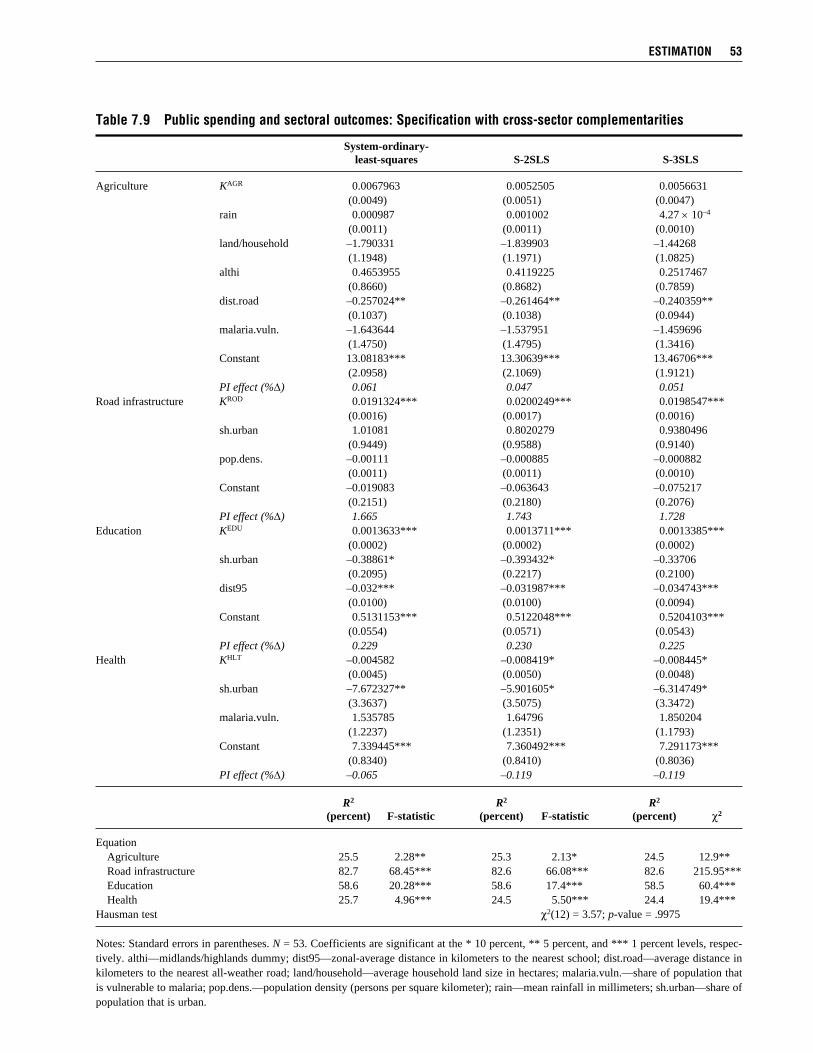
estimation 53
table 7.9 Public spending and sectoral outcomes: specification with cross-sector complementarities
System-ordinary- least-squares S-2SLS S-3SLS
Agriculture KAGR 0.0067963 0.0052505 0.0056631 (0.0049) (0.0051) (0.0047) rain 0.000987 0.001002 4.27 × 10⁻⁴
(0.0011) (0.0011) (0.0010) land/household –1.790331 –1.839903 –1.44268 (1.1948) (1.1971) (1.0825) althi 0.4653955 0.4119225 0.2517467 (0.8660) (0.8682) (0.7859) dist.road –0.257024** –0.261464** –0.240359** (0.1037) (0.1038) (0.0944) malaria.vuln. –1.643644 –1.537951 –1.459696 (1.4750) (1.4795) (1.3416) Constant 13.08183*** 13.30639*** 13.46706*** (2.0958) (2.1069) (1.9121) PI effect (%∆) 0.061 0.047 0.051Road infrastructure KROD 0.0191324*** 0.0200249*** 0.0198547*** (0.0016) (0.0017) (0.0016) sh.urban 1.01081 0.8020279 0.9380496 (0.9449) (0.9588) (0.9140) pop.dens. –0.00111 –0.000885 –0.000882 (0.0011) (0.0011) (0.0010) Constant –0.019083 –0.063643 –0.075217 (0.2151) (0.2180) (0.2076) PI effect (%∆) 1.665 1.743 1.728Education KEDU 0.0013633*** 0.0013711*** 0.0013385*** (0.0002) (0.0002) (0.0002) sh.urban –0.38861* –0.393432* –0.33706 (0.2095) (0.2217) (0.2100) dist95 –0.032*** –0.031987*** –0.034743*** (0.0100) (0.0100) (0.0094) Constant 0.5131153*** 0.5122048*** 0.5204103*** (0.0554) (0.0571) (0.0543) PI effect (%∆) 0.229 0.230 0.225Health KHLT –0.004582 –0.008419* –0.008445* (0.0045) (0.0050) (0.0048) sh.urban –7.672327** –5.901605* –6.314749* (3.3637) (3.5075) (3.3472) malaria.vuln. 1.535785 1.64796 1.850204 (1.2237) (1.2351) (1.1793) Constant 7.339445*** 7.360492*** 7.291173*** (0.8340) (0.8410) (0.8036) PI effect (%∆) –0.065 –0.119 –0.119
R2 R2 R2 (percent) F-statistic (percent) F-statistic (percent) χ2
Equation Agriculture 25.5 2.28** 25.3 2.13* 24.5 12.9** Road infrastructure 82.7 68.45*** 82.6 66.08*** 82.6 215.95*** Education 58.6 20.28*** 58.6 17.4*** 58.5 60.4*** Health 25.7 4.96*** 24.5 5.50*** 24.4 19.4***Hausman test χ2(12) = 3.57; p-value = .9975
Notes: Standard errors in parentheses. N = 53. Coefficients are significant at the * 10 percent, ** 5 percent, and *** 1 percent levels, respec-tively. althi—midlands/highlands dummy; dist95—zonal-average distance in kilometers to the nearest school; dist.road—average distance in kilometers to the nearest all-weather road; land/household—average household land size in hectares; malaria.vuln.—share of population that is vulnerable to malaria; pop.dens.—population density (persons per square kilometer); rain—mean rainfall in millimeters; sh.urban—share of population that is urban.

54 CHaPteR 7
table 7.10 Public spending and sectoral outcomes: specification including agricultural inputs as a determinant of agricultural productivity
System-ordinary- least-squares S-2SLS S-3SLS
Agriculture KAGR 0.0058733 0.0043099 0.0041859 (0.0048) (0.0050) (0.0045) rain 0.0015426 0.0015783 0.00123 (0.0012) (0.0012) (0.0010) land/household –2.345597* –2.429116** –2.267958** (1.2243) (1.2276) (1.0693) althi –0.144644 –0.207076 –0.3148728 (0.9056) (0.9080) (0.7901) sh.seed 7.134519 6.174791 1.310289 (13.8322) (13.8694) (12.1705) sh.irrig. 6.409159** 6.583235** 7.429033*** (2.7522) (2.7590) (2.4094) sh.pest. 8.436073 8.529788 7.03293 (6.5303) (6.5396) (5.6997) sh.fert. 1.906399 1.923865 1.945616 (2.8582) (2.8622) (2.5043) Constant 9.30266*** 9.593535*** 10.10134*** (1.7483) (1.7640) (1.5466) PI effect (%∆) 0.052 0.038 0.037Road infrastructure KROD 0.0191324*** 0.0198417*** 0.019815*** (0.0016) (0.0017) (0.0016) sh.urban 1.01081 0.8448688 0.8389041 (0.9449) (0.9565) (0.9141) pop.dens. –0.00111 –0.000931 –0.0008942 (0.0011) (0.0011) (0.0010) Constant –0.019083 –0.054499 –0.0569279 (0.2151) (0.2175) (0.2073) PI effect (%∆) 1.665 1.727 1.725Education KEDU 0.0013633*** 0.0014382*** 0.0013977*** (0.0002) (0.0002) (0.0002) sh.urban –0.38861* –0.43503** –0.380588* (0.2095) (0.2169) (0.2046) dist95 –0.032*** –0.03187*** –0.034046*** (0.0100) (0.0100) (0.0094) Constant 0.5131153*** 0.50435*** 0.5123307*** (0.0554) (0.0565) (0.0536) PI effect (%∆) 0.229 0.242 0.235Health KHLT –0.004582 –0.008506* –0.0084996* (0.0045) (0.0048) (0.0046) sh.urban –7.672327** –5.86153* –6.20289* (3.3637) (3.4647) (3.2904) malaria.vuln. 1.535785 1.650498 1.664079 (1.2237) (1.2351) (1.1696) Constant 7.339445*** 7.360968*** 7.401786*** (0.8340) (0.8413) (0.7994) PI effect (%∆) –0.06 –0.120 –0.120
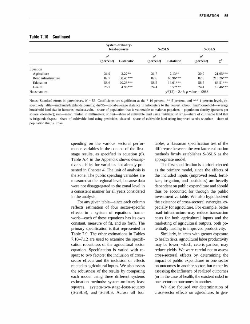
spending on the various sectoral perfor-mance variables in the context of the first-stage results, as specified in equation (6). Table A.4 in the Appendix shows descrip-tive statistics for variables not already pre-sented in Chapter 4. The unit of analysis is the zone. The public spending variables are measured at the regional level, because data were not disaggregated to the zonal level in a consistent manner for all years considered in the analysis. For any given table—since each column reflects estimation of four sector-specific effects in a system of equations frame-work—each of these equations has its own constant, measure of fit, and so forth. The primary specification is that represented in Table 7.9. The other estimations in Tables 7.10–7.12 are used to examine the specifi-cation robustness of the agricultural sector equation. Specification is varied with re-spect to two factors: the inclusion of cross-sector effects and the inclusion of effects related to agricultural inputs. We also assess the robustness of the results by comparing each model using three different systems estimation methods: system-ordinary least squares, system-two-stage-least-squares (S-2SLS), and S-3SLS. Across all four
estimation 55
table 7.10 Continued
System-ordinary- least-squares S-2SLS S-3SLS
R2 R2 R2 (percent) F-statistic (percent) F-statistic (percent) χ2
Equation Agriculture 31.9 2.22** 31.7 2.13** 30.0 21.05*** Road infrastructure 82.7 68.45*** 82.6 65.96*** 82.6 216.26*** Education 58.6 20.28*** 58.5 19.61*** 58.5 66.51*** Health 25.7 4.96*** 24.4 5.57*** 24.4 19.46***Hausman test χ2(12) = 2.46; p-value = .9983
Notes: Standard errors in parentheses. N = 53. Coefficients are significant at the * 10 percent, ** 5 percent, and *** 1 percent levels, re-spectively. althi—midlands/highlands dummy; dist95—zonal-average distance in kilometers to the nearest school; land/household—average household land size in hectares; malaria.vuln.—share of population that is vulnerable to malaria; pop.dens.—population density (persons per square kilometer); rain—mean rainfall in millimeters; sh.fert—share of cultivable land using fertilizer; sh.irrig—share of cultivable land that is irrigated; sh.pest—share of cultivable land using pesticides; sh.seed—share of cultivable land using improved seeds; sh.urban—share of population that is urban.
tables, a Hausman specification test of the difference between the two latter estimation methods firmly establishes S-3SLS as the appropriate model. The first specification is a priori selected as the primary model, since the effects of the included inputs (improved seed, fertil-izer, irrigation, and pesticides) are heavily dependent on public expenditure and should thus be accounted for through the public investment variable. We also hypothesized the existence of cross-sectoral synergies, es-pecially for agriculture. For example, better road infrastructure may reduce transaction costs for both agricultural inputs and the marketing of agricultural outputs, both po-tentially leading to improved productivity. Similarly, in areas with greater exposure to health risks, agricultural labor productivity may be lower, which, ceteris paribus, may reduce yields. We were careful not to assess cross-sectoral effects by determining the impact of public expenditure in one sector on outcomes in another sector, but rather by assessing the influence of realized outcomes (or in the case of health, the existent risks) in one sector on outcomes in another. We also focused our determination of cross-sector effects on agriculture. In gen-
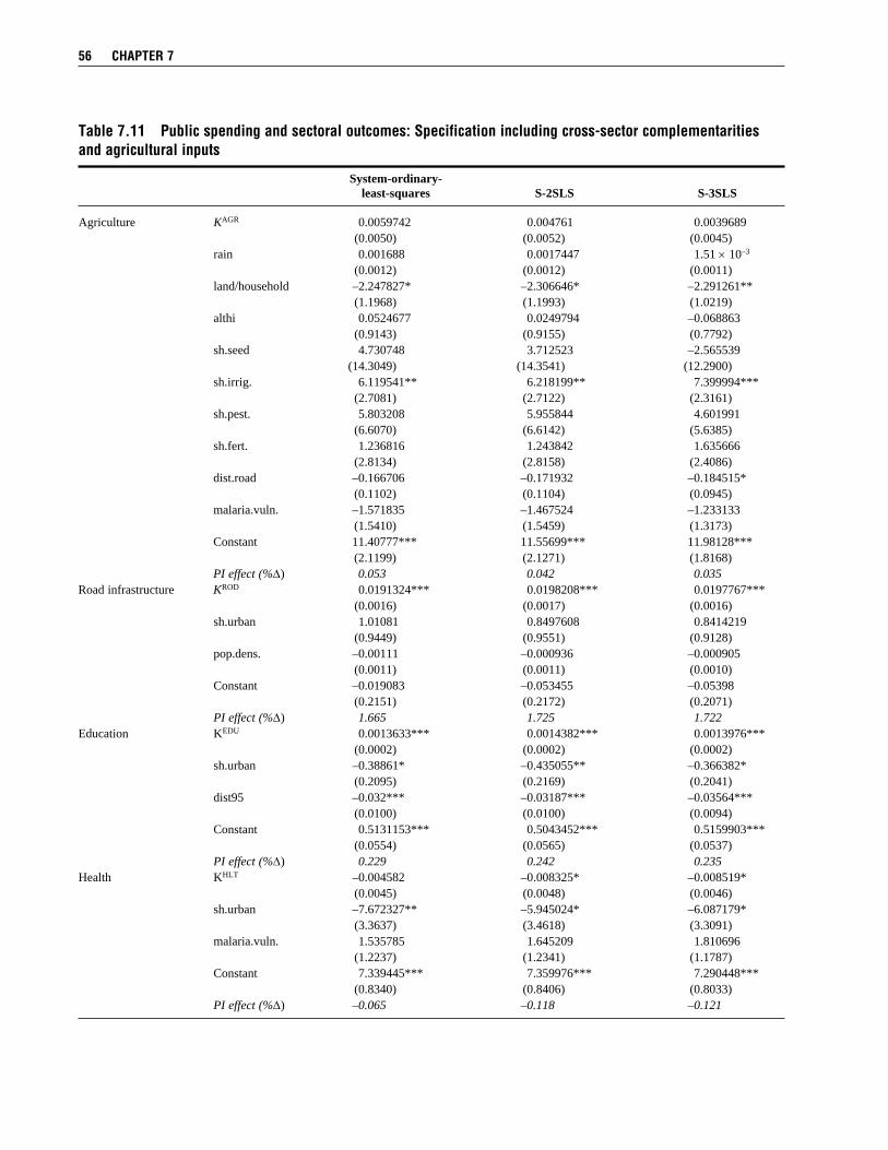
56 CHaPteR 7
table 7.11 Public spending and sectoral outcomes: specification including cross-sector complementarities and agricultural inputs
System-ordinary- least-squares S-2SLS S-3SLS
Agriculture KAGR 0.0059742 0.004761 0.0039689 (0.0050) (0.0052) (0.0045) rain 0.001688 0.0017447 1.51 × 10⁻³
(0.0012) (0.0012) (0.0011) land/household –2.247827* –2.306646* –2.291261** (1.1968) (1.1993) (1.0219) althi 0.0524677 0.0249794 –0.068863 (0.9143) (0.9155) (0.7792) sh.seed 4.730748 3.712523 –2.565539 (14.3049) (14.3541) (12.2900) sh.irrig. 6.119541** 6.218199** 7.399994*** (2.7081) (2.7122) (2.3161) sh.pest. 5.803208 5.955844 4.601991 (6.6070) (6.6142) (5.6385) sh.fert. 1.236816 1.243842 1.635666 (2.8134) (2.8158) (2.4086) dist.road –0.166706 –0.171932 –0.184515* (0.1102) (0.1104) (0.0945) malaria.vuln. –1.571835 –1.467524 –1.233133 (1.5410) (1.5459) (1.3173) Constant 11.40777*** 11.55699*** 11.98128*** (2.1199) (2.1271) (1.8168) PI effect (%∆) 0.053 0.042 0.035Road infrastructure KROD 0.0191324*** 0.0198208*** 0.0197767*** (0.0016) (0.0017) (0.0016) sh.urban 1.01081 0.8497608 0.8414219 (0.9449) (0.9551) (0.9128) pop.dens. –0.00111 –0.000936 –0.000905 (0.0011) (0.0011) (0.0010) Constant –0.019083 –0.053455 –0.05398 (0.2151) (0.2172) (0.2071) PI effect (%∆) 1.665 1.725 1.722Education KEDU 0.0013633*** 0.0014382*** 0.0013976*** (0.0002) (0.0002) (0.0002) sh.urban –0.38861* –0.435055** –0.366382* (0.2095) (0.2169) (0.2041) dist95 –0.032*** –0.03187*** –0.03564*** (0.0100) (0.0100) (0.0094) Constant 0.5131153*** 0.5043452*** 0.5159903*** (0.0554) (0.0565) (0.0537) PI effect (%∆) 0.229 0.242 0.235Health KHLT –0.004582 –0.008325* –0.008519* (0.0045) (0.0048) (0.0046) sh.urban –7.672327** –5.945024* –6.087179* (3.3637) (3.4618) (3.3091) malaria.vuln. 1.535785 1.645209 1.810696 (1.2237) (1.2341) (1.1787) Constant 7.339445*** 7.359976*** 7.290448*** (0.8340) (0.8406) (0.8033) PI effect (%∆) –0.065 –0.118 –0.121
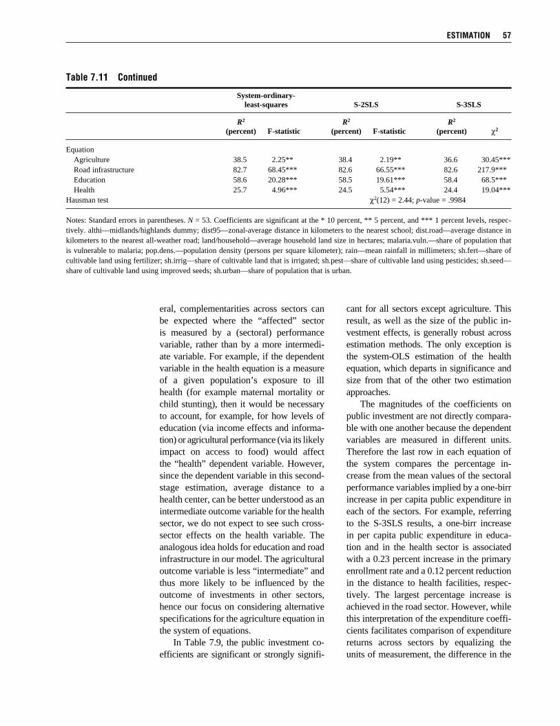
eral, complementarities across sectors can be expected where the “affected” sector is measured by a (sectoral) performance variable, rather than by a more intermedi-ate variable. For example, if the dependent variable in the health equation is a measure of a given population’s exposure to ill health (for example maternal mortality or child stunting), then it would be necessary to account, for example, for how levels of education (via income effects and informa- tion) or agricultural performance (via its likely impact on access to food) would affect the “health” dependent variable. However, since the dependent variable in this second- stage estimation, average distance to a health center, can be better understood as an intermediate outcome variable for the health sector, we do not expect to see such cross-sector effects on the health variable. The analogous idea holds for education and road infrastructure in our model. The agricultural outcome variable is less “intermediate” and thus more likely to be influenced by the outcome of investments in other sectors, hence our focus on considering alternative specifications for the agriculture equation in the system of equations. In Table 7.9, the public investment co- efficients are significant or strongly signifi-
cant for all sectors except agriculture. This result, as well as the size of the public in-vestment effects, is generally robust across estimation methods. The only exception is the system-OLS estimation of the health equation, which departs in significance and size from that of the other two estimation approaches. The magnitudes of the coefficients on public investment are not directly compara-ble with one another because the dependent variables are measured in different units. Therefore the last row in each equation of the system compares the percentage in-crease from the mean values of the sectoral performance variables implied by a one-birr increase in per capita public expenditure in each of the sectors. For example, referring to the S-3SLS results, a one-birr increase in per capita public expenditure in educa-tion and in the health sector is associated with a 0.23 percent increase in the primary enrollment rate and a 0.12 percent reduction in the distance to health facilities, respec-tively. The largest percentage increase is achieved in the road sector. However, while this interpretation of the expenditure coeffi-cients facilitates comparison of expenditure returns across sectors by equalizing the units of measurement, the difference in the
estimation 57
table 7.11 Continued
System-ordinary- least-squares S-2SLS S-3SLS
R2 R2 R2 (percent) F-statistic (percent) F-statistic (percent) χ2
Equation Agriculture 38.5 2.25** 38.4 2.19** 36.6 30.45*** Road infrastructure 82.7 68.45*** 82.6 66.55*** 82.6 217.9*** Education 58.6 20.28*** 58.5 19.61*** 58.4 68.5*** Health 25.7 4.96*** 24.5 5.54*** 24.4 19.04***Hausman test χ2(12) = 2.44; p-value = .9984
Notes: Standard errors in parentheses. N = 53. Coefficients are significant at the * 10 percent, ** 5 percent, and *** 1 percent levels, respec-tively. althi—midlands/highlands dummy; dist95—zonal-average distance in kilometers to the nearest school; dist.road—average distance in kilometers to the nearest all-weather road; land/household—average household land size in hectares; malaria.vuln.—share of population that is vulnerable to malaria; pop.dens.—population density (persons per square kilometer); rain—mean rainfall in millimeters; sh.fert—share of cultivable land using fertilizer; sh.irrig—share of cultivable land that is irrigated; sh.pest—share of cultivable land using pesticides; sh.seed—share of cultivable land using improved seeds; sh.urban—share of population that is urban.
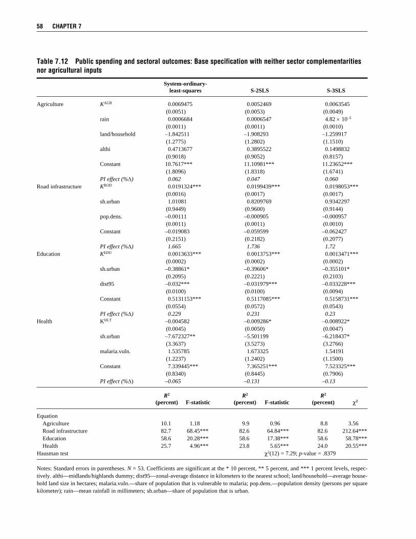
58 CHaPteR 7
table 7.12 Public spending and sectoral outcomes: Base specification with neither sector complementarities nor agricultural inputs
System-ordinary- least-squares S-2SLS S-3SLS
Agriculture KAGR 0.0069475 0.0052469 0.0063545 (0.0051) (0.0053) (0.0049) rain 0.0006684 0.0006547 4.82 × 10⁻⁵
(0.0011) (0.0011) (0.0010) land/household –1.842511 –1.908293 –1.259917 (1.2775) (1.2802) (1.1510) althi 0.4713677 0.3895522 0.1498832 (0.9018) (0.9052) (0.8157) Constant 10.7617*** 11.10981*** 11.23652*** (1.8096) (1.8318) (1.6741) PI effect (%∆) 0.062 0.047 0.060Road infrastructure KROD 0.0191324*** 0.0199439*** 0.0198053*** (0.0016) (0.0017) (0.0017) sh.urban 1.01081 0.8209769 0.9342297 (0.9449) (0.9600) (0.9144) pop.dens. –0.00111 –0.000905 –0.000957 (0.0011) (0.0011) (0.0010) Constant –0.019083 –0.059599 –0.062427 (0.2151) (0.2182) (0.2077) PI effect (%∆) 1.665 1.736 1.72Education KEDU 0.0013633*** 0.0013753*** 0.0013471*** (0.0002) (0.0002) (0.0002) sh.urban –0.38861* –0.39606* –0.355101* (0.2095) (0.2221) (0.2103) dist95 –0.032*** –0.031979*** –0.033228*** (0.0100) (0.0100) (0.0094) Constant 0.5131153*** 0.5117085*** 0.5158731*** (0.0554) (0.0572) (0.0543) PI effect (%∆) 0.229 0.231 0.23Health KHLT –0.004582 –0.009286* –0.008922* (0.0045) (0.0050) (0.0047) sh.urban –7.672327** –5.501199 –6.218437* (3.3637) (3.5273) (3.2766) malaria.vuln. 1.535785 1.673325 1.54191 (1.2237) (1.2402) (1.1500) Constant 7.339445*** 7.365251*** 7.523325*** (0.8340) (0.8445) (0.7906) PI effect (%∆) –0.065 –0.131 –0.13
R2 R2 R2 (percent) F-statistic (percent) F-statistic (percent) χ2
Equation Agriculture 10.1 1.18 9.9 0.96 8.8 3.56 Road infrastructure 82.7 68.45*** 82.6 64.84*** 82.6 212.64*** Education 58.6 20.28*** 58.6 17.38*** 58.6 58.78*** Health 25.7 4.96*** 23.8 5.65*** 24.0 20.55***Hausman test χ2(12) = 7.29; p-value = .8379
Notes: Standard errors in parentheses. N = 53. Coefficients are significant at the * 10 percent, ** 5 percent, and *** 1 percent levels, respec-tively. althi—midlands/highlands dummy; dist95—zonal-average distance in kilometers to the nearest school; land/household—average house-hold land size in hectares; malaria.vuln.—share of population that is vulnerable to malaria; pop.dens.—population density (persons per square kilometer); rain—mean rainfall in millimeters; sh.urban—share of population that is urban.

underlying outcome variables means that these figures are still indicative only of the comparative contribution of spending in the different sectors. By assessing household welfare effects, the third-stage estimation, discussed subsequently, allows for more direct comparability. Examining the results across model specifications, that is across Tables 7.9–7.12, we see that the results of the three nonag-ricultural sectors are very stable vis-à-vis the changes in specification in the agricul- ture equation (for system-OLS they are of course identical). The coefficients in the ag-riculture equation are also relatively stable. The coefficient on the variable of interest, agricultural spending, is somewhat reduced when agricultural inputs are included (for example comparing Table 7.11 with Table 7.9, and comparing Table 7.10 with Table 7.12). This is quite intuitive, as the provi-sion of agricultural inputs and infrastruc-ture, such as fertilizer, seeds, and irrigation, is in great part enabled through public ex-penditures in agriculture. The results for the second-stage analysis presented so far are based on public invest-ment variables derived from equation (5) as-suming a depreciation rate and discount rate of d = 0.05 and r = 0.05, respectively. It is useful to examine whether there are impor-tant qualitative changes in the core findings concerning the effect of public investments in the four sectors, or whether these results fundamentally hold. Table 7.13 gives a sum- mary of the public investment coefficients for different parametric assumptions. The co- efficients are presented for each of the three systems estimation methods and the four specifications of the agriculture equation that correspond to the specifications in Tables 7.9–7.12. Tables A.5–A.8 in the Appendix present the full results for these alternative parametric assumptions, based on the main variable specification (the specifi-cation as in Table 7.9). Changing the magnitude of the depre-ciation and discount rate parameters within
the range of 2–10 percent has important consequences for the public investment ef-fects. Increasing these parameters increases the (absolute value of the) public investment coefficients by a factor of anywhere from 1.5 to 4. Varying the depreciation rate increases the coefficients by more than varying the discount rate by the same magnitude. For example, assuming d = 0.02 and increasing r from 0.02 to 0.10 results in an increase of the public investment coefficient by 53 percent, 47 percent, 59 percent, and 81 per- cent for the agriculture, road infrastruc-ture, education, and health sectors, respec-tively (based on the main variable specifica-tion and 3SLS estimation). But increasing the depreciation rate value from 2 percent to 10 percent, holding the discount rate at 2 percent, increases the four respective co- efficients by 90 percent, 81 percent, 106 per- cent, and 161 percent. The qualitative impact of these differ-ent parameter assumptions follows from equation (5): an increase in either parameter reduces the cumulative public investment in any given sector, so that the marginal effect of public investment in the regression will be higher. What is not as immediate is the way in which changing these assumptions may affect inferences on the coefficients and the stability of the results with changing specifications. Table 7.13 and Tables A.5– A.8 in the Appendix show that our core results are highly robust to varying the pa-rameter assumptions.
Third-Stage Analysis: Linking Household Welfare to Public SpendingAs discussed in Chapter 5, the third- stage estimation draws on the first two stages of the analysis by using equation (9) to assess the effect on rural house- hold consumption of a marginal increase in per capita public expenditure in various sectors. In Table 7.14 the first column draws on the first stage’s main specification
estimation 59

60 CHaPteR 7
table 7.13 Public spending and sectoral outcomes: summary of public investment coefficients for different parametric assumptions
System- System- ordinary- ordinary-Specification/sector least-squares S-2SLS S-3SLS least-squares S-2SLS S-3SLS
d = 0.02, r = 0.02 d = 0.10, r = 0.10
C Agriculture 0.00448* 0.00339 0.00348 0.00734 0.00575 0.00670 Road infrastructure 0.01176*** 0.01298*** 0.01292*** 0.02430*** 0.02509*** 0.02478*** Education 0.00079*** 0.00082*** 0.00080*** 0.00183*** 0.00182*** 0.00180*** Health –0.00231* –0.00423* –0.00436* –0.00715 –0.01340* –0.01307*I Agriculture 0.00359 0.00265 0.00239 0.00693 0.00470 0.00467 Road infrastructure 0.01176*** 0.01267*** 0.01276*** 0.02430*** 0.02490*** 0.02475*** Education 0.00079*** 0.00086*** 0.00084*** 0.00183*** 0.00191*** 0.00187*** Health –0.00231 –0.00423* –0.00435* –0.00715 –0.01356* –0.01314*CI Agriculture 0.00385 0.00300 0.00237 0.00650 0.00511 0.00418 Road infrastructure 0.01176*** 0.01263*** 0.01268*** 0.02430*** 0.02488*** 0.02473*** Education 0.00079*** 0.00086*** 0.00084*** 0.00183*** 0.00191*** 0.00186*** Health –0.00231 –0.00413* –0.00435* –0.00715 –0.01334* –0.01330*B Agriculture 0.00423 0.00305 0.00367 0.00835 0.00632 0.00790 Road infrastructure 0.01176*** 0.01290*** 0.01291*** 0.02430*** 0.02503*** 0.02474*** Education 0.00079*** 0.00083*** 0.00081*** 0.00183*** 0.00182*** 0.00180*** Health –0.00231 –0.00466* –0.00459* –0.00715 –0.01474* –0.01368*
d = 0.02, r = 0.10 d = 0.10, r = 0.02
C Agriculture 0.00634 0.00497 0.00533 0.00771 0.00590 0.00662 Road infrastructure 0.01834*** 0.01921*** 0.01904*** 0.02275*** 0.02358*** 0.02334*** Education 0.00129*** 0.00130*** 0.00127*** 0.00169*** 0.00168*** 0.00165*** Health –0.00430 –0.00787* –0.00789* –0.00619 –0.01152* –0.01138*I Agriculture 0.00557 0.00413 0.00405 0.00683 0.00478 0.00466 Road infrastructure 0.01834*** 0.01905*** 0.01901*** 0.02275*** 0.02338*** 0.02330*** Education 0.00129*** 0.00137*** 0.00133*** 0.00169*** 0.00176*** 0.00172*** Health –0.00430 –0.00795* –0.00793* –0.00619 –0.01166* –0.01146*CI Agriculture 0.00565 0.00455 0.00384 0.00650 0.00511 0.00418 Road infrastructure 0.01834*** 0.01904*** 0.01899*** 0.02430*** 0.02488*** 0.02473*** Education 0.00129*** 0.00137*** 0.00133*** 0.00183*** 0.00191*** 0.00186*** Health –0.00430 –0.00778* –0.00795* –0.00715 –0.01334* –0.01330*B Agriculture 0.00653 0.00499 0.00601 0.00823 0.00616 0.00759 Road infrastructure 0.01834*** 0.01913*** 0.01899*** 0.02275*** 0.02351*** 0.02330*** Education 0.00129*** 0.00131*** 0.00128*** 0.00169*** 0.00168*** 0.00165*** Health –0.00430 –0.00868* –0.00835* –0.00619 –0.01269* –0.01195*
Notes: Abbreviations for specifications: B = base assumption, without complementarities and agricultural inputs; C = complementarities across sector investments; CI = cross-sector complementarities and agricultural inputs included; I = agricultural inputs included.
(Table 7.6) and the second column uses the average-effects regression (Table 7.7) for comparison.
While the first-stage regression showed that two regions seem to stand out in terms of the strong effect that access to roads ap-
peared to have on consumption, the third stage allows the effect of road infrastructure expenditure on household consumption to be quantified. For example, a one-birr in-crease in per capita expenditure on roads in Afar is found to lead to a five-birr increase

estimation 61
table 7.14 impact of public expenditure on household welfare: two alternative first-stage specifications
Based on second stage’s specification C, main estimation (S-3SLS), and d = 0.05, r = 0.05
First stage: Direct First stage: and indirect effects Average effects
Agriculture Afar 0.0104 0.0485 (0.028) (0.080) Amhara 0.0465 –0.00210 (0.056) (0.070) Beneshangul-Gumuz 0.2313 0.0561 (0.314) (0.564) Dire Dawa 0.2971 0.5650 (0.251) (0.478) Gambela 0.0457 0.0294 (0.110) (0.091) Harari 0.3915 0.8555 (0.336) (0.718) Oromia 0.0757 0.3703 (0.068) (0.314) SNNP 0.1811 0.0019 (0.151) (0.099) Somale –0.1139 0.9052 (0.247) (0.827) Tigray 0.1986 0.0664 (0.178) (0.178)Road infrastructure Afar 5.0390*** 8.1533*** (1.527) (1.995) Amhara 11.9514*** 11.2656*** (2.922) (3.644) Beneshangul-Gumuz –0.6973 –3.0122 (3.477) (4.013) Gambela 0.1909 0.3524 (0.499) (0.540) Oromia 1.2293 –4.7474* (2.258) (2.948) SNNP –2.5089*** –4.4274*** (0.667) (1.059) Somale 14.3842* –5.9852 (8.519) (8.818) Tigray 4.1785 0.8858 (3.389) (4.139)Education Afar 1.8786** –0.1400 (0.777) (0.815) Amhara 0.1710 0.8305** (0.149) (0.299) Beneshangul-Gumuz 0.0149 1.1243 (0.114) (1.147) Dire Dawa 0.5202** — (0.218)
(continued )
in per capita consumption of rural house-holds in this region.3
The effects of spending on agriculture and health should be interpreted with cau-tion, given that the standard errors obtained via the delta method are large. Nevertheless
some tentative findings can be established. The strongest effects of spending appear to be associated with rural households in the city-states Dire Dawa and Harari. In these locations a one-birr increase in spending results in greater than 0.39 and 0.29 birr in-
62 CHaPteR 7
table 7.14 Continued
Based on second stage’s specification C, main estimation (S-3SLS), and d = 0.05, r = 0.05
First stage: Direct First stage: and indirect effects Average effects
Gambela –0.2410** — (0.101) Harari 0.5951*** — (0.194) Oromia 0.5254*** –0.0700 (0.164) (0.293) SNNP –0.0300 1.1826** (0.115) (0.458) Somale 2.0312*** — (0.660) Tigray 0.1073 1.0026* (0.122) (0.542)Health Afar 0.0715* 0.0667 (0.044) (0.049) Amhara 0.0251 –0.0005 (0.033) (0.035) Beneshangul-Gumuz 0.0171 0.0256 (0.026) (0.041) Dire Dawa –0.1776 –0.1923 (0.157) (0.181) Gambela –0.1035 –0.1380 (0.076) (0.097) Harari –0.1307 –0.0548 (0.223) (0.231) Oromia –0.0251 –0.0431 (0.034) (0.046) SNNP 0.0256 –0.0235 (0.037) (0.038) Somale –0.0574 –0.0654 (0.057) (0.066) Tigray 0.0245 –0.0559 (0.052) (0.070)
Notes: Standard errors in parentheses. Coefficients are significant at the * 10 percent, ** 5 percent, and *** 1 percent levels, respectively. Abbreviation for specification: C—complementarities across sector investments. — indicates that an estimate of the coefficient could not be derived due to collinearity. SNNP—Southern Nations, Nation-alities, and Peoples.
3For ease of interpretation, the first-stage coefficients were first transformed so the third-stage results reflect the impact of spending on per-adult-equivalent household expenditure, rather than its log.

creases in per capita household consumption for the two regions, respectively. In com-parison with the results on road expenditure, returns to agricultural expenditures, though not uniform, tend to be much more stable across regions than returns to spending on road infrastructure. What is also noticeable, however, is that the highest returns to road spending are substantially higher than the highest returns to agricultural spending. The returns to public spending on edu-cation appear to be larger than those to agricultural expenditure, but they still fall substantially short of the investment returns for road infrastructure, although the former are significant for more regions. As with the level of returns, the interregional variation of the returns to education spending lies between that in agriculture and road infra-structure. Similar to the case of agriculture, significant results were not observed with regard to rural welfare returns to health spending. Unlike the agricultural sector, however, the results from the first-stage regression are weak for most regions. This is not inconsistent with the findings of Collier, Dercon, and Mackinnon (2002), who reported that in Ethiopia the returns to public expenditure on the “quantity” of health care (which is what our measure of access to public services captures) are very low, especially in comparison to invest-ments in the “quality” of health care. It is certainly of note that the results give not just significant and low but even nega-tive coefficients for SNNP and Gambela related to returns to road infrastructure and education spending, respectively. This find-ing arises from the first-stage analysis of the impact of sectoral performance on rural welfare. As discussed previously in the context of this first stage, this is likely to be due to the limitation of the partial analysis offered by this study: while road infrastructure, for example, may serve rural and urban residents alike, we are only considering its effects on rural households’ incomes. Furthermore the design of pub-lic investments, for example in education, may serve purposes other than increasing
income, including enhancing equity and meeting certain social goals—outcomes that may in some cases constitute a trade-off to increases in average income, and outcomes that are not captured in this study. This may suggest the need for additional work, in-cluding the consideration of other potential outcomes (beyond rural income) that may result from improvements in sector-specific performance indicators. Finally Tables 7.15 and 7.16 extend to this third-stage analysis the previous robust-ness checks against different values for the depreciation and discount rate parameters in equation (5), and against exclusion of sets of observations associated with regions, respec-tively. With regard to the discount and depre-ciation rate sensitivity analysis, we find again that the core interpretation of the coefficients summarized earlier holds when deriving re-sults for varying parameter assumptions. On the other hand, Table 7.16 shows that results on returns to spending in the educa-tion sector are affected when observations of two regions are (separately) excluded. Excluding the data on either Afar or Oromia renders the returns to education expenditures significant (as well as higher in magnitude) in Amhara and Tigray; they are nonsignifi-cant in the base model. Put another way, in-clusion of households in the Oromia region will tend to “hide” the confidence in the results on the returns to education spending in certain other regions, and analogously for the case of inclusion of Afar in the analysis. Results for the other three sectors are not affected to any great degree by the exclusion regressions (unlike the analogous case in the first stage; compare with Table 7.8). With returns in the education sector in the base model already statistically significant across more regions than the other sectors, the data robustness analysis presents findings that, if anything, lend additional confidence to the conclusion that the returns to education investments seem to be widely dispersed across Ethiopia, even if returns to infrastruc-ture spending, which are more concentrated, are larger in magnitude where they are found to be statistically significant.
estimation 63

table 7.15 impact of public expenditure on household welfare: Four alternative second-stage parameter value assumptions
Based on first stage’s main specification (direct and indirect effects) and second stage’s specification C (with cross-sector effects) and second stage’s main estimation (S-3SLS)
d = 0.02, r = 0.02 d = 0.02, r = 0.10 d = 0.10, r = 0.02 d = 0.10, r = 0.10
Agriculture Afar 0.0064 0.0098 0.0121 0.012 (0.017) (0.027) (0.034) (0.035) Amhara 0.0285 0.0438 0.0543 0.055 (0.032) (0.053) (0.071) (0.077) Beneshangul-Gumuz 0.1421 0.2179 0.2704 0.273 (0.181) (0.295) (0.389) (0.416) Dire Dawa 0.1825 0.2799 0.3474 0.351 (0.129) (0.234) (0.336) (0.382) Gambela 0.0281 0.0431 0.0535 0.054 (0.066) (0.103) (0.131) (0.135) Harari 0.2405 0.3688 0.4577 0.463 (0.174) (0.313) (0.449) (0.508) Oromia 0.0465 0.0713 0.0885 0.089 (0.036) (0.063) (0.090) (0.101) SNNP 0.1112 0.1706 0.2117 0.214 (0.077) (0.141) (0.203) (0.231) Somale –0.0700 –0.1073 –0.1332 –0.135 (0.148) (0.232) (0.296) (0.306) Tigray 0.1220 0.1871 0.2322 0.235 (0.094) (0.167) (0.236) (0.265)Road infrastructure Afar 3.2793*** 4.8327*** 5.9228*** 6.290*** (0.995) (1.466) (1.797) (1.912) Amhara 7.7778*** 11.4621*** 14.0477*** 14.918*** (1.904) (2.806) (3.440) (3.665) Beneshangul-Gumuz –0.4538 –0.6688 –0.8196 –0.870 (2.263) (3.335) (4.087) (4.340) Gambela 0.1242 0.1831 0.2244 0.238 (0.325) (0.479) (0.587) (0.623) Oromia 0.8000 1.1789 1.4449 1.534 (1.470) (2.166) (2.654) (2.819) SNNP –1.6327*** –2.4062*** –2.9489*** –3.132*** (0.435) (0.641) (0.785) (0.836) Somale 9.3610* 13.7952* 16.9071* 17.954* (5.545) (8.172) (10.016) (10.642) Tigray 2.7193 4.0074 4.9114 5.216 (2.206) (3.250) (3.984) (4.232)Education Afar 1.1294** 1.7877** 2.3113** 2.522** (0.468) (0.739) (0.956) (1.043)
64 CHaPteR 7
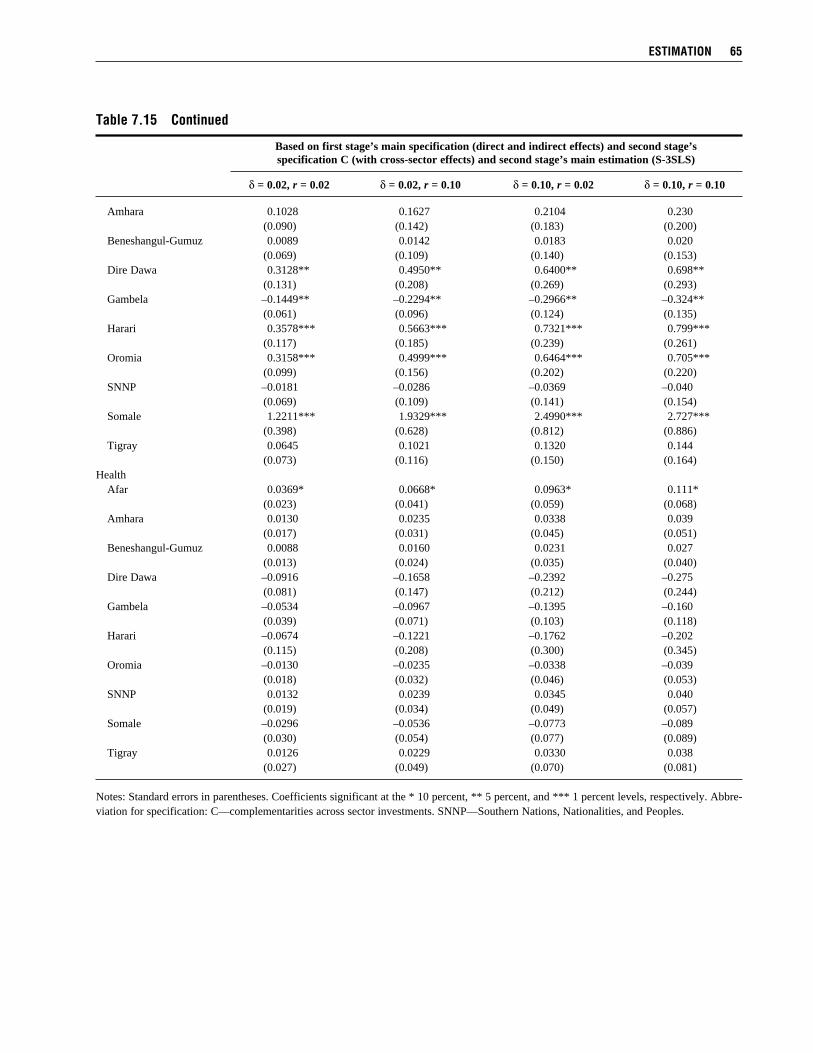
estimation 65
table 7.15 Continued
Based on first stage’s main specification (direct and indirect effects) and second stage’s specification C (with cross-sector effects) and second stage’s main estimation (S-3SLS)
d = 0.02, r = 0.02 d = 0.02, r = 0.10 d = 0.10, r = 0.02 d = 0.10, r = 0.10
Amhara 0.1028 0.1627 0.2104 0.230 (0.090) (0.142) (0.183) (0.200) Beneshangul-Gumuz 0.0089 0.0142 0.0183 0.020 (0.069) (0.109) (0.140) (0.153) Dire Dawa 0.3128** 0.4950** 0.6400** 0.698** (0.131) (0.208) (0.269) (0.293) Gambela –0.1449** –0.2294** –0.2966** –0.324** (0.061) (0.096) (0.124) (0.135) Harari 0.3578*** 0.5663*** 0.7321*** 0.799*** (0.117) (0.185) (0.239) (0.261) Oromia 0.3158*** 0.4999*** 0.6464*** 0.705*** (0.099) (0.156) (0.202) (0.220) SNNP –0.0181 –0.0286 –0.0369 –0.040 (0.069) (0.109) (0.141) (0.154) Somale 1.2211*** 1.9329*** 2.4990*** 2.727*** (0.398) (0.628) (0.812) (0.886) Tigray 0.0645 0.1021 0.1320 0.144 (0.073) (0.116) (0.150) (0.164)Health Afar 0.0369* 0.0668* 0.0963* 0.111* (0.023) (0.041) (0.059) (0.068) Amhara 0.0130 0.0235 0.0338 0.039 (0.017) (0.031) (0.045) (0.051) Beneshangul-Gumuz 0.0088 0.0160 0.0231 0.027 (0.013) (0.024) (0.035) (0.040) Dire Dawa –0.0916 –0.1658 –0.2392 –0.275 (0.081) (0.147) (0.212) (0.244) Gambela –0.0534 –0.0967 –0.1395 –0.160 (0.039) (0.071) (0.103) (0.118) Harari –0.0674 –0.1221 –0.1762 –0.202 (0.115) (0.208) (0.300) (0.345) Oromia –0.0130 –0.0235 –0.0338 –0.039 (0.018) (0.032) (0.046) (0.053) SNNP 0.0132 0.0239 0.0345 0.040 (0.019) (0.034) (0.049) (0.057) Somale –0.0296 –0.0536 –0.0773 –0.089 (0.030) (0.054) (0.077) (0.089) Tigray 0.0126 0.0229 0.0330 0.038 (0.027) (0.049) (0.070) (0.081)
Notes: Standard errors in parentheses. Coefficients significant at the * 10 percent, ** 5 percent, and *** 1 percent levels, respectively. Abbre-viation for specification: C—complementarities across sector investments. SNNP—Southern Nations, Nationalities, and Peoples.

tabl
e 7.
16
impa
ct o
f pub
lic e
xpen
ditu
re o
n ho
useh
old
wel
fare
: Rob
ustn
ess
to e
xclu
sion
of o
bser
vatio
ns
Exc
lude
d
B
enes
hang
ul-
obse
rvat
ions
N
one
Afa
r A
mha
ra
Gum
uz
Dir
e D
awa
Gam
bela
H
arar
i O
rom
ia
SNN
P
Som
ale
Tig
ray
Roa
d in
fras
truc
ture
A
far
5.03
90**
* —
5.
0305
***
5.07
30**
* 5.
0252
***
5.03
30**
* 5.
0107
***
4.94
20**
* 5.
1791
***
5.02
50**
* 4.
9817
***
(1
.527
)
(1.4
77)
(1.5
15)
(1.5
36)
(1.5
31)
(1.5
35)
(1.5
74)
(1.4
97)
(1.5
4)
(1.5
21)
A
mha
ra
11.9
514*
**
11.5
320*
**
—
11.6
263*
**
12.2
009*
**
12.0
233*
**
12.2
056*
**
12.7
115*
**
10.9
605*
**
12.2
519*
**
12.3
236*
**
(2.9
22)
(2.9
11)
(2
.916
) (2
.933
) (2
.924
) (2
.929
) (2
.948
) (2
.948
) (2
.928
) (2
.933
)
Ben
esha
ngul
-Gum
uz
–0.6
973
–0.6
213
–0.1
970
—
–0.8
917
–0.7
529
–0.8
961
–1.3
466
–0.0
830
–0.9
247
–0.7
394
(3
.477
) (3
.495
) (3
.536
)
(3.4
59)
(3.4
71)
(3.4
63)
(3.4
58)
(3.5
18)
(3.4
57)
(3.4
77)
G
ambe
la
0.19
09
0.17
93
0.27
88
0.21
76
0.16
32
—
0.16
70
0.12
45
0.21
64
0.16
80
0.20
02
(0.4
99)
(0.5
) (0
.495
) (0
.497
) (0
.501
)
(0.5
) (0
.502
) (0
.499
) (0
.501
) (0
.499
)
Oro
mia
1.
2293
1.
3448
0.
6568
1.
0397
1.
3912
1.
2315
1.
4399
—
0.
7509
1.
4154
1.
1827
(2
.258
) (2
.256
) (2
.236
) (2
.25)
(2
.273
) (2
.26)
(2
.27)
(2.2
55)
(2.2
69)
(2.2
66)
SN
NP
–2.5
089*
**
–2.5
428*
**
–2.4
991*
**
–2.5
653*
**
–2.5
022*
**
–2.5
055*
**
–2.4
821*
**
–2.3
484*
**
—
–2.4
668*
**
–2.4
996*
**
(0.6
67)
(0.6
57)
(0.7
) (0
.68)
(0
.662
) (0
.665
) (0
.658
) (0
.626
)
(0.6
53)
(0.6
65)
So
mal
e 14
.384
2*
15.6
577*
12
.903
6*
13.9
622*
14
.669
7*
14.4
798*
14
.737
1*
16.3
984*
11
.862
3*
—
14.2
440*
(8
.519
) (8
.663
) (8
.197
) (8
.37)
(8
.614
) (8
.549
) (8
.64)
(9
.034
) (8
.07)
(8.5
12)
T
igra
y 4.
1785
4.
0300
4.
1368
4.
2606
4.
1669
4.
1573
4.
1777
4.
0504
4.
2889
4.
1405
—
(3
.389
) (3
.381
) (3
.355
) (3
.404
) (3
.388
) (3
.388
) (3
.388
) (3
.375
) (3
.393
) (3
.389
) A
gric
ultu
re
Afa
r 0.
0104
—
0.
0120
0.
0052
0.
0117
0.
0110
0.
0129
0.
0215
–0
.005
9 0.
0133
0.
0128
(0
.028
)
(0.0
29)
(0.0
28)
(0.0
29)
(0.0
29)
(0.0
29)
(0.0
33)
(0.0
29)
(0.0
29)
(0.0
29)
A
mha
ra
0.04
65
0.04
35
—
0.03
87
0.05
02
0.04
76
0.05
12
0.06
74
0.02
37
0.05
25
0.04
75
(0.0
56)
(0.0
55)
(0
.052
) (0
.059
) (0
.057
) (0
.059
) (0
.07)
(0
.047
) (0
.06)
(0
.057
)
Ben
esha
ngul
-Gum
uz
0.23
13
0.21
76
0.19
68
—
0.24
78
0.23
57
0.24
83
0.28
71
0.17
49
0.25
10
0.23
50
(0.3
14)
(0.3
08)
(0.3
01)
(0
.321
) (0
.316
) (0
.322
) (0
.343
) (0
.291
) (0
.323
) (0
.316
)
Dir
e D
awa
0.29
71
0.28
04
0.30
13
0.28
87
—
0.29
82
0.30
10
0.30
89
0.28
04
0.30
17
0.29
99
(0.2
51)
(0.2
38)
(0.2
54)
(0.2
44)
(0
.252
) (0
.254
) (0
.261
) (0
.237
) (0
.255
) (0
.253
)
Gam
bela
0.
0457
0.
0412
0.
0341
0.
0387
0.
0513
—
0.
0507
0.
0590
0.
0383
0.
0506
0.
0447
(0
.11)
(0
.109
) (0
.106
) (0
.108
) (0
.112
)
(0.1
12)
(0.1
15)
(0.1
08)
(0.1
12)
(0.1
1)
Har
ari
0.39
15
0.36
77
0.39
95
0.38
13
0.39
52
0.39
24
—
0.40
47
0.37
28
0.39
60
0.39
53
(0.3
36)
(0.3
18)
(0.3
41)
(0.3
27)
(0.3
39)
(0.3
36)
(0
.349
) (0
.32)
(0
.34)
(0
.339
)
Oro
mia
0.
0757
0.
0653
0.
0863
0.
0741
0.
0750
0.
0757
0.
0749
—
0.
0743
0.
0751
0.
0774
(0
.068
) (0
.061
) (0
.076
) (0
.067
) (0
.067
) (0
.068
) (0
.067
)
(0.0
67)
(0.0
67)
(0.0
69)
SN
NP
0.18
11
0.17
30
0.18
08
0.17
74
0.18
33
0.18
15
0.18
35
0.18
63
—
0.18
33
0.18
41
(0.1
51)
(0.1
45)
(0.1
51)
(0.1
48)
(0.1
53)
(0.1
51)
(0.1
53)
(0.1
55)
(0
.153
) (0
.153
)
Som
ale
–0.1
139
–0.1
678
–0.0
639
–0.1
110
–0.1
196
–0.1
157
–0.1
210
–0.1
584
–0.0
611
—
–0.1
068
(0
.247
) (0
.271
) (0
.225
) (0
.243
) (0
.252
) (0
.248
) (0
.253
) (0
.276
) (0
.225
)
(0.2
46)
T
igra
y 0.
1986
0.
1894
0.
1911
0.
1886
0.
2036
0.
2002
0.
2042
0.
2221
0.
1655
0.
2069
—
(0
.178
) (0
.172
) (0
.172
) (0
.171
) (0
.182
) (0
.18)
(0
.183
) (0
.197
) (0
.154
) (0
.185
)
66 CHaPteR 7

Hea
lth
Afa
r 0.
0715
* —
0.
0743
* 0.
0736
* 0.
0711
* 0.
0713
* 0.
0710
* 0.
0631
* 0.
0811
* 0.
0694
* 0.
0735
*
(0.0
44)
(0
.046
) (0
.045
) (0
.044
) (0
.044
) (0
.044
) (0
.04)
(0
.049
) (0
.043
) (0
.045
)
Am
hara
0.
0251
0.
0225
—
0.
0263
0.
0251
0.
0251
0.
0247
0.
0201
0.
0327
0.
0237
0.
0257
(0
.033
) (0
.032
)
(0.0
34)
(0.0
33)
(0.0
33)
(0.0
33)
(0.0
31)
(0.0
36)
(0.0
33)
(0.0
33)
B
enes
hang
ul-G
umuz
0.
0171
0.
0174
0.
0185
—
0.
0168
0.
0170
0.
0169
0.
0147
0.
0189
0.
0168
0.
0167
(0
.026
) (0
.026
) (0
.026
)
(0.0
26)
(0.0
26)
(0.0
26)
(0.0
25)
(0.0
26)
(0.0
26)
(0.0
26)
D
ire
Daw
a –0
.177
6 –0
.178
0 –0
.174
0 –0
.176
0 —
–0
.178
0 –0
.178
6 –0
.179
7 –0
.181
5 –0
.177
1 –0
.175
3
(0.1
57)
(0.1
56)
(0.1
54)
(0.1
56)
(0
.158
) (0
.158
) (0
.16)
(0
.157
) (0
.158
) (0
.157
)
Gam
bela
–0
.103
5 –0
.104
2 –0
.099
9 –0
.102
7 –0
.104
0 —
–0
.104
2 –0
.104
6 –0
.103
9 –0
.104
2 –0
.103
2
(0.0
76)
(0.0
76)
(0.0
74)
(0.0
75)
(0.0
77)
(0
.077
) (0
.077
) (0
.076
) (0
.077
) (0
.076
)
Har
ari
–0.1
307
–0.1
285
–0.1
191
–0.1
271
–0.1
342
–0.1
318
—
–0.1
437
–0.1
177
–0.1
352
–0.1
334
(0
.223
) (0
.222
) (0
.22)
(0
.222
) (0
.223
) (0
.223
)
(0.2
24)
(0.2
19)
(0.2
24)
(0.2
25)
O
rom
ia
–0.0
251
–0.0
269
–0.0
236
–0.0
243
–0.0
252
–0.0
253
–0.0
254
—
–0.0
221
–0.0
257
–0.0
245
(0
.034
) (0
.035
) (0
.034
) (0
.034
) (0
.034
) (0
.034
) (0
.034
)
(0.0
33)
(0.0
34)
(0.0
34)
SN
NP
0.02
56
0.02
19
0.03
19
0.02
89
0.02
44
0.02
49
0.02
37
0.01
34
—
0.02
21
0.02
53
(0.0
37)
(0.0
36)
(0.0
38)
(0.0
37)
(0.0
36)
(0.0
36)
(0.0
36)
(0.0
34)
(0
.036
) (0
.036
)
Som
ale
–0.0
574
–0.0
601
–0.0
535
–0.0
575
–0.0
568
–0.0
572
–0.0
580
–0.0
612
–0.0
529
—
–0.0
578
(0
.057
) (0
.059
) (0
.056
) (0
.057
) (0
.057
) (0
.057
) (0
.058
) (0
.06)
(0
.055
)
(0.0
57)
T
igra
y 0.
0245
0.
0216
0.
0215
0.
0247
0.
0256
0.
0244
0.
0253
0.
0225
0.
0279
0.
0244
—
(0
.052
) (0
.052
) (0
.053
) (0
.053
) (0
.052
) (0
.052
) (0
.052
) (0
.051
) (0
.053
) (0
.052
) E
duca
tion
A
far
1.87
86**
—
1.
7307
**
1.72
03**
1.
9201
**
1.89
61**
1.
9519
**
2.42
41**
1.
2061
* 2.
0203
**
1.82
65**
(0
.777
)
(0.7
71)
(0.7
66)
(0.7
81)
(0.7
79)
(0.7
84)
(0.8
53)
(0.7
31)
(0.7
92)
(0.7
72)
A
mha
ra
0.17
10
0.23
44+
* —
0.
1382
0.
1758
0.
1736
0.
1823
0.
2978
+*
0.01
08
0.20
29
0.14
72
(0.1
49)
(0.1
54)
(0
.15)
(0
.15)
(0
.149
) (0
.15)
(0
.161
) (0
.151
) (0
.151
) (0
.149
)
Ben
esha
ngul
-Gum
uz
0.01
49
0.06
21
–0.0
176
—
0.02
06
0.01
70
0.02
49
0.10
45
–0.0
978
0.03
98
–0.0
005
(0
.114
) (0
.114
) (0
.12)
(0.1
14)
(0.1
14)
(0.1
14)
(0.1
16)
(0.1
21)
(0.1
14)
(0.1
15)
D
ire
Daw
a 0.
5202
**
0.60
43**
0.
4584
**
0.47
69**
—
0.
5242
**
0.53
94**
0.
7034
**
0.28
74
0.56
68**
0.
5019
**
(0.2
18)
(0.2
27)
(0.2
16)
(0.2
15)
(0
.219
) (0
.222
) (0
.246
) (0
.2)
(0.2
25)
(0.2
18)
G
ambe
la
–0.2
410*
* –0
.203
3**
–0.2
707*
* –0
.263
2**
–0.2
330*
* —
–0
.232
1**
–0.1
616*
–0
.345
8***
–0
.216
6**
–0.2
494*
*
(0.1
01)
(0.0
99)
(0.1
07)
(0.1
03)
(0.1
01)
(0
.101
) (0
.099
) (0
.112
) (0
.1)
(0.1
02)
H
arar
i 0.
5951
***
0.64
74**
* 0.
5632
***
0.57
10**
* 0.
5987
***
0.59
75**
* —
0.
6939
***
0.46
43**
0.
6218
***
0.58
23**
*
(0.1
94)
(0.2
) (0
.189
) (0
.191
) (0
.196
) (0
.195
)
(0.2
13)
(0.1
78)
(0.1
99)
(0.1
94)
O
rom
ia
0.52
54**
* 0.
6001
***
0.45
64**
0.
4785
***
0.53
98**
* 0.
5298
***
0.54
86**
* —
0.
3067
**
0.57
28**
* 0.
5061
***
(0
.164
) (0
.174
) (0
.166
) (0
.161
) (0
.167
) (0
.165
) (0
.167
)
(0.1
47)
(0.1
7)
(0.1
63)
SN
NP
–0.0
300
0.03
98
–0.0
750
–0.0
681
–0.0
206
–0.0
270
–0.0
149
0.11
66
—
0.01
01
–0.0
518
(0
.115
) (0
.117
) (0
.124
) (0
.118
) (0
.116
) (0
.115
) (0
.116
) (0
.126
)
(0.1
16)
(0.1
16)
So
mal
e 2.
0312
***
2.28
26**
* 1.
8021
**
1.86
95**
2.
0790
***
2.05
00**
* 2.
1124
***
2.64
59**
* 1.
2795
**
—
1.96
23**
*
(0.6
6)
(0.6
94)
(0.6
56)
(0.6
49)
(0.6
7)
(0.6
64)
(0.6
74)
(0.7
56)
(0.6
)
(0.6
57)
T
igra
y 0.
1073
0.
1607
0.
0566
0.
0794
0.
1145
0.
1104
0.
1215
0.
2244
+*
–0.0
492
0.13
93
—
(0.1
22)
(0.1
25)
(0.1
27)
(0.1
23)
(0.1
24)
(0.1
23)
(0.1
23)
(0.1
34)
(0.1
22)
(0.1
24)
Not
es:
Coe
ffic
ient
s ar
e si
gnif
ican
t at
the
* 1
0 pe
rcen
t, **
5 p
erce
nt,
and
***
1 pe
rcen
t le
vels
, re
spec
tivel
y. —
ind
icat
es n
ot a
pplic
able
. SN
NP—
Sout
hern
Nat
ions
, N
atio
nalit
ies,
and
Peo
ples
. +
den
otes
no
ntri
vial
cha
nges
fro
m th
e ba
se m
odel
.
estimation 67

C H A P T E R 8
Conclusions and Policy Considerations
In this report we explored and compared the impact of different types of public spending on rural household welfare in Ethiopia. In order to get at this question empirically, we used a three-stage analysis: the first stage assessed the role of access to different sector-specific
services and outcomes for rural household consumption, differentiating this effect geographi-cally as well as tracing the effect that public services have on the productivity of household private assets. The second stage of the analysis determined the contribution of different types of public spending on key sector-specific outcomes, accounting both for the fact that this contribution is usually realized over time and for the fact that public expenditure volumes in a given sector may be affected by the state of development in that sector. The final stage of the analysis drew on results from the two previous stages to estimate the rural welfare effect of a unit increase in public spending across different sectors. We find that, among the sectors considered, returns to public investments in road infra-structure are by far the highest. However, the geographic variability of welfare returns to public spending on roads is also higher than that in other sectors. This regional variability in returns to road investment suggests the need for careful region-specific investment policies in the road sector. Tentative evidence also suggests that higher returns are seen in areas having better-developed road networks and that the converse is also true. The presence of increasing returns to road investments, while not conclusive, may provide guidance for public policy in trading off the potentially higher gains from geographic concentration of road networks against equity concerns in the provision of infrastructure. The household welfare impacts of public expenditure in agriculture are smaller than the ef-fects of road spending, and they also did not emerge as statistically significant. The results of the first- and second-stage analyses suggest that the lack of significance derives from the poor link from public expenditures to performance of the agricultural sector, and not from a limited role of agriculture in rural welfare. The first-stage analysis shows in fact that performance of the agricultural sector contributes significantly to rural consumption both when considering this role on average for Ethiopia as a whole and when assessing regionally disaggregated effects. Comparison of the impact of agricultural expenditures across regions shows that the larg-est returns are observed in two small regions that are each dominated by a major city. While proximity to markets is not explicitly analyzed herein, we suggest that the relatively high returns to agricultural spending for rural residents in the two most urbanized regions may be capturing the important role of market proximity in determining the effectiveness of public investments in agriculture. However, these findings can only be stated tentatively, given the low statistical significance associated with the third-stage results. In contrast to the road infrastructure sector, returns to expenditures in education are char-acterized by wider reach, more homogeneity, and less intensity. Education spending has wide-
68

spread effects on welfare, in that these re-turns are positive, significant, and similar across a broad range of regions, in con-trast to the stronger concentration within a few regions of returns to expenditures in the road sector. This finding is further strengthened in robustness checks of the main results with regard to exclusion of sets of observations. The magnitude of returns to education spending is more constrained than in the road sector, but still larger and more significant than that of returns to in-vestments in agriculture. Rural welfare re-turns to spending in the health sector do not emerge strongly, with significant findings in only one region, and the magnitude of the birr-for-birr returns is relatively low. Some useful steps may be taken to fur-ther strengthen any conclusions arising from this analysis and provide new insights into the relative effectiveness of different types of public spending. First, the public expen-diture and household data used in this study extend only to 2000. This was the most recent year for which public spending data were available at the time the data for this research were collected, and the most recent HICE survey also covered 1999/2000. A useful extension of this research would be to repeat the analysis for more recent years, when the composition of spending in Ethio-pia saw important changes. Second, while this report assesses how rural household consumption is affected by public expenditure, our findings may also be used to simulate the poverty effects of public spending. Third, given the promi-nence of agriculture-driven development in Ethiopia’s current poverty reduction strat-egy, it may not be doing full justice to the policy dimension of this inquiry to examine the impact of public expenditure in the aggregate. Additional studies may be war-ranted to examine separately the role of
the various components of this investment, such as agricultural extension, agricultural research, and food security spending. At present the lack of regionally disaggregated time series data on spending in the various agricultural subsectors necessitates analy-sis of agricultural expenditure as a whole. Future efforts in collecting additional data from the regional bureaus of agriculture and others would alleviate this constraint. However, cross-sector comparisons of re-turns to agricultural spending with returns to education, infrastructure, and other spend-ing would call for a similar subsectoral or functional disaggregation of spending in these other sectors, to maintain symmetry in analysis. An issue that goes beyond the scope of this report but is clearly worthy of ad-ditional study is the efficiency of public spending. The utility of public investments for household welfare and poverty reduc-tion depends on at least two things: (1) the portfolio of the public budget, or the ap-propriateness of the allocation of resources across sectors, and (2) the efficiency with which resources are used in any given sec-tor or subsector. This report focused on the former issue. In a way the results of this report provoke an inquiry into the second question, and they do so pointedly in the Ethiopian context, with respect to agri- cultural investments. This is both because agriculture strongly dominates Ethiopia’s economy and because the government’s de-velopment strategy emphasizes the agricul-tural sector. A substantial body of research suggests that a strategic focus on agriculture may be appropriate given Ethiopia’s stage of development (for example Diao et al. 2007). Therefore an investigation into the drivers of efficiency in the country’s agricultural public spending may be the next important step in policy research in Ethiopia.
conclusions and policy considerations 69

A p p e n d i x
70
SomaleOromia
Tigray
Amhara
SUDAN
ERITREA
SOMALIA
DJIBOUTI
SOMALIA
KENYA
Gambela
SNNP
Benes
hang
ul-
Gum
uz
Afar
Addis Ababa
DireDawa
Harari
1 50 100 150 200 km
N
Figure A.1 Administrative map of Ethiopia
Source: Based on data from the United Nations Office for the Co-ordination of Humanitarian Affairs.Note: SNNP—Southern Nations, Nationalities, and Peoples.

AppEndix 71
Table A.1 per capita household expenditure, based on the Household income, Consumption and Expenditure (HiCE) Surveys
Rural growth, Total Urban Rural 1995 rural 1995–99 (percent)
Addis Ababa 2,465.7 2,482.9 1,540.4 1,685.9 –8.6Afar 1,537.7 2,302.0 1,127.0 1,520.5 –25.9Amhara 1,165.6 1,754.4 1,095.7 974.4 12.4Beneshangul-Gumuz 1,158.3 2,014.3 1,088.4 1,075.0 1.3Dire Dawa 1,767.0 1,899.3 1,394.4 1,682.8 –17.1Gambela 1,330.3 1,898.1 1,255.7 1,706.7 –26.4Harari 1,904.9 2,106.2 1,618.7 2,388.7 –32.2Oromia 1,208.4 1,701.0 1,144.5 1,282.9 –10.8SNNP 1,080.1 1,768.9 1,025.2 1,021.3 0.4Somale 1,626.7 2,106.7 1,395.1 1,975.4 –29.4Tigray 1,189.5 1,536.7 1,120.9 1,209.6 –7.3Ethiopia 1,222.5 1,921.0 1,109.9 1,136.6 –2.3
Source: Central Statistical Authority (2001).Note: SNNP—Southern Nations, Nationalities, and Peoples.
1999
Table A.2 per-adult-equivalent household expenditure, based on the Welfare Monitoring Surveys
Growth Region Zones 1995 1999 (percent)
Addis Ababa 1,543.3 1,521.0 –1.4Afar 2,038.6 1,770.1 –13.2Amhara 1 East and West Gojam, Agawi 1,493.4 1,937.8 29.8Amhara 2 North and South Gondar 1,264.0 1,629.2 28.9Amhara 3 North Wollo, Wag Hamra 1,211.1 1,430.1 18.1Amhara 4 South Wollo, Oromiya, North Shewa 1,483.3 1,501.8 1.2Beneshangul-Gumuz 1,296.7 1,347.0 3.9Dire Dawa 1,595.9 1,573.9 –1.4Gambela 1,464.3 1,021.6 –30.2Harari 2,615.7 1,901.4 –27.3Oromia 1 East and West Hararghe 2,087.8 1,631.3 –21.9Oromia 2 East and West Wellega 1,732.9 1,809.7 4.4Oromia 3 East Shewa, Arsi, Bale, Borena 1,664.4 1,599.8 –3.9Oromia 4 Illubabor, Jimma 1,893.4 1,501.4 –20.7Oromia 5 North and West Shewa 1,965.1 1,928.8 –1.8SNNP 1 Hadiya, Kambata, Gurage 1,319.9 1,197.3 –9.3SNNP 2 North and South Omo, Derashe, Konso 1,708.0 2,059.0 20.5SNNP 3 Sidama, Gedeo, Burji, Amaro 1,257.8 1,106.9 –12.0SNNP 4 Yem, Keficho, Maji, Shekicho, Bench 1,492.9 1,514.9 1.5Somale 2,597.2 2,313.3 –10.9Tigray 1,412.8 1,409.9 –0.2
Source: World Bank (2005d).Note: SNNP—Southern Nations, Nationalities, and Peoples.

72 AppEndix
Tabl
e A.
3 S
pend
ing
in e
ach
regi
on, 1
998
(per
cent
of t
otal
regi
onal
exp
endi
ture
s)
A
ddis
B
enes
hang
ul-
Dir
e
R
egio
nal
A
baba
A
far
Am
hara
G
umuz
D
awa
Gam
bela
H
arar
i O
rom
ia
SNN
P
Som
ale
Tig
ray
tota
l
Roa
ds
27.4
3.
8 17
.8
5.1
0.0
3.0
0.0
22.4
10
.5
5.2
4.7
100.
0E
duca
tion
7.9
2.6
21.9
2.
0 0.
9 2.
9 1.
0 33
.7
18.3
2.
7 6.
2 10
0.0
Hea
lth
8.4
4.5
21.7
3.
8 1.
2 2.
3 1.
9 23
.6
15.4
5.
1 12
.1
100.
0A
gric
ultu
re
1.0
4.1
23.4
2.
9 0.
6 1.
0 0.
3 31
.0
25.2
5.
5 4.
9 10
0.0
Nat
ural
res
ourc
es
27.8
13
.1
13.8
1.
5 0.
3 0.
4 0.
4 22
.2
8.8
2.8
8.9
100.
0E
nerg
y an
d m
inin
g 0.
0 0.
5 51
.6
1.0
5.5
0.0
11.4
3.
5 0.
7 0.
0 25
.9
100.
0T
rans
port
atio
n an
d co
mm
unic
atio
ns
26.6
4.
1 14
.6
3.7
6.5
0.0
0.0
41.4
0.
3 2.
6 0.
2 10
0.0
Oth
er
24.3
6.
3 16
.4
4.5
1.9
2.4
1.2
16.5
13
.8
7.0
5.7
100.
0T
otal
15
.8
5.1
19.4
3.
4 1.
1 2.
2 1.
0 24
.8
15.8
4.
9 6.
6 10
0.0
Popu
latio
n 3.
9 1.
9 25
.6
0.8
0.5
0.3
0.3
35.2
19
.7
5.8
5.8
100.
0
Sour
ce: A
utho
rs’
own
calc
ulat
ions
usi
ng d
ata
from
Min
istr
y of
Fin
ance
and
Eco
nom
ic D
evel
opm
ent.
Not
e: S
NN
P—So
uthe
rn N
atio
ns, N
atio
nalit
ies,
and
Peo
ples
.
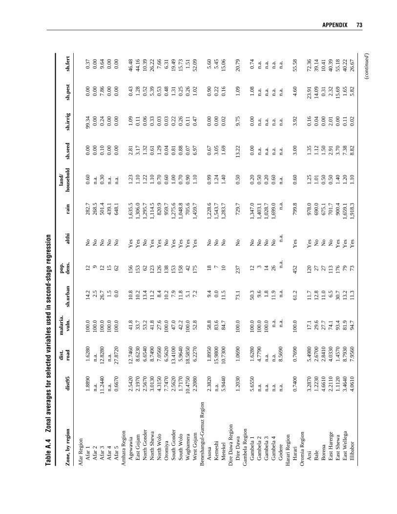
AppEndix 73
Tabl
e A.
4 Z
onal
ave
rage
s fo
r sel
ecte
d va
riabl
es u
sed
in s
econ
d-st
age
regr
essi
on
dist
. m
alar
ia.
po
p.
land
/
Zon
e, b
y re
gion
di
st95
ro
ad
vuln
. sh
.urb
an
dens
. al
thi
rain
ho
useh
old
sh.s
eed
sh.ir
rig
sh.p
est
sh.f
ert
Afa
r R
egio
n
Afa
r 1
1.88
90
1.62
80
100.
0 14
.2
12
No
282.
7 0.
60
0.00
99
.34
0.00
0.
37
Afa
r 2
n.a.
n.
a.
100.
0 2.
5 9
No
268.
5 n.
a.
0.00
0.
00
0.00
0.
00
Afa
r 3
11.2
440
12.8
280
100.
0 26
.7
12
No
501.
4 0.
30
0.10
0.
24
7.86
9.
64
Afa
r 4
n.a.
n.
a.
100.
0 1.
5 15
N
o 43
9.1
n.a.
0.
00
0.00
0.
00
0.00
A
far
5 0.
6670
27
.872
0 10
0.0
0.0
62
No
648.
1 n.
a.
0.00
0.
00
0.00
0.
00A
mha
ra R
egio
n
Age
waw
ia
2.54
20
12.7
460
41.8
10
.8
156
Yes
1,
635.
5 1.
23
2.81
1.
09
0.43
46
.48
E
ast G
ojam
2.
1970
8.
6230
33
.7
10.2
15
3 Y
es
1,30
6.0
1.10
3.
17
0.11
1.
28
44.1
6
Nor
th G
onde
r 2.
5670
6.
6540
53
.2
13.4
62
N
o 1,
295.
7 1.
22
1.32
0.
06
0.52
10
.39
N
orth
She
wa
3.01
30
8.74
90
41.8
11
.2
123
Yes
1,
114.
5 1.
10
0.61
0.
33
5.39
26
.22
N
orth
Wol
o 4.
3150
7.
0560
27
.6
8.4
126
Yes
82
0.9
0.70
1.
29
0.03
0.
53
7.66
O
rom
iya
7.74
70
6.56
20
100.
0 10
.2
138
No
959.
7 0.
60
0.04
0.
03
0.48
6.
31
Sout
h G
onde
r 2.
5620
13
.410
0 47
.0
7.9
153
Yes
1,
275.
6 1.
00
0.81
0.
22
1.31
19
.49
So
uth
Wol
o 1.
7170
5.
9640
42
.2
11.8
15
8 Y
es
1,04
8.8
0.70
0.
88
0.26
0.
25
15.7
3
Wag
ham
era
10.4
750
18.5
850
100.
0 5.
1 42
Y
es
705.
6 0.
90
0.07
0.
11
0.26
1.
51
Wes
t Goj
am
2.20
80
6.22
70
52.8
7.
2 17
5 Y
es
1,45
9.7
1.10
6.
97
0.47
1.
02
52.0
9B
enes
hang
ul-G
umuz
Reg
ion
A
sosa
2.
3820
1.
8950
58
.8
9.4
18
No
1,22
8.6
0.99
0.
67
0.00
0.
90
5.60
K
emes
hi
n.a.
15
.980
0 83
.6
0.0
7 N
o 1,
543.
7 1.
24
3.05
0.
00
0.22
5.
45
Met
ekel
5.
9440
10
.730
0 84
.7
11.5
10
N
o 1,
283.
7 1.
40
1.69
0.
02
0.16
15
.06
Dir
e D
awa
Reg
ion
D
ire
Daw
a 1.
2030
1.
0690
10
0.0
73.1
23
7 N
o 72
9.7
0.50
13
.22
9.75
1.
09
20.7
9G
ambe
la R
egio
n
Gam
bela
1
5.65
50
1.62
80
100.
0 50
.3
12
No
1,34
7.0
0.20
0.
00
0.00
1.
08
0.74
G
ambe
la 2
n.
a.
4.77
90
100.
0 9.
6 3
No
1,40
3.1
0.50
n.
a.
n.a.
n.
a.
n.a.
G
ambe
la 3
n.
a.
n.a.
10
0.0
1.8
14
No
1,02
8.7
0.20
n.
a.
n.a.
n.
a.
n.a.
G
ambe
la 4
n.
a.
n.a.
n.
a.
11.9
26
N
o 1,
699.
0 0.
60
n.a.
n.
a.
n.a.
n.
a.
God
ere
n.a.
8.
5690
n.
a.
n.a.
n.
a.
n.a.
n.
a.
n.a.
n.
a.
n.a.
n.
a.
n.a.
Har
ari R
egio
n
Har
ari
0.74
00
0.76
90
100.
0 61
.2
452
Yes
79
9.8
0.60
3.
00
3.92
4.
60
55.5
8O
rom
ia R
egio
n
Ars
i 3.
2870
5.
4980
17
.1
11.7
12
0 Y
es
978.
0 1.
25
1.35
0.
16
23.9
1 72
.36
B
ale
1.22
30
2.67
00
29.6
12
.8
27
No
690.
0 1.
01
1.12
0.
04
14.0
9 39
.14
B
oren
a 4.
6610
2.
8410
27
.7
11.0
27
N
o 67
5.1
0.50
1.
50
0.00
0.
31
10.4
1
Eas
t Har
erge
2.
2110
4.
0330
74
.1
6.5
113
No
701.
7 0.
50
2.91
2.
01
2.32
40
.39
E
ast S
hew
a 1.
1120
1.
4570
93
.4
30.7
17
6 Y
es
900.
4 1.
40
3.70
0.
00
15.6
9 55
.18
E
ast W
elle
ga
3.46
40
8.79
30
81.9
13
.2
79
Yes
1,
659.
1 1.
20
7.38
0.
11
1.65
40
.22
Il
libab
or
4.06
10
7.95
60
94.7
11
.3
73
Yes
1,
918.
3 1.
10
8.82
0.
02
5.82
26
.67
(con
tinu
ed)

74 AppEndixTa
ble
A.4
Con
tinue
d
dist
. m
alar
ia.
po
p.
land
/
Zon
e, b
y re
gion
di
st95
ro
ad
vuln
. sh
.urb
an
dens
. al
thi
rain
ho
useh
old
sh.s
eed
sh.ir
rig
sh.p
est
sh.f
ert
Ji
mm
a 2.
2720
6.
1120
29
.5
11.6
14
7 Y
es
1,66
6.4
0.90
5.
60
0.00
22
.25
36.0
7
Nor
th S
hew
a 3.
4120
5.
7910
35
.9
8.9
138
No
1,60
0.4
1.20
1.
00
0.10
4.
79
29.7
6
Wes
t Har
erge
3.
0080
2.
1780
68
.5
9.1
98
Yes
88
5.0
0.70
1.
62
1.36
0.
32
16.9
3
Wes
t She
wa
3.07
40
4.06
00
17.6
11
.6
150
Yes
1,
288.
4 1.
20
2.87
0.
23
26.1
3 56
.43
W
est W
elle
ga
4.44
50
6.77
90
69.5
10
.3
86
No
1,60
0.4
1.00
6.
84
0.17
1.
56
30.3
7SN
NP
Reg
ion
A
mar
o 3.
5420
12
.120
0 10
0.0
3.7
93
Yes
92
7.0
0.40
0.
87
9.80
1.
91
8.50
B
ench
-Maj
i 3.
6800
6.
5310
18
.0
8.6
18
No
1,29
6.8
0.30
2.
00
0.00
0.
00
7.00
B
urji
2.20
80
3.60
70
100.
0 13
.6
33
No
964.
0 0.
70
0.24
0.
00
2.03
6.
33
Der
ashe
5.
0000
6.
2080
10
0.0
10.8
86
N
o 1,
113.
0 0.
80
0.02
3.
49
0.27
0.
90
Ged
io
1.71
00
3.12
50
57.7
13
.7
505
Yes
1,
564.
8 0.
30
1.87
0.
00
0.00
31
.17
G
urag
e 3.
6290
5.
6980
20
.0
5.9
239
Yes
1,
111.
4 0.
50
10.4
9 0.
09
10.7
8 61
.80
H
adiy
a 2.
5370
4.
4290
43
.9
7.7
371
Yes
1,
148.
0 0.
60
6.35
0.
02
33.6
6 82
.82
K
efic
ho-S
hek.
2.
6050
12
.238
0 34
.0
9.2
71
Yes
1,
886.
9 0.
70
1.00
0.
00
5.00
5.
00
Kem
bata
2.
3040
4.
6850
59
.4
8.4
395
Yes
1,
089.
3 0.
60
6.21
0.
00
18.5
7 71
.94
K
onso
1.
6470
4.
2890
10
0.0
4.2
88
No
878.
0 0.
60
0.00
2.
66
0.03
30
.55
N
orth
Om
o 3.
3470
8.
4940
77
.4
8.1
144
Yes
1,
463.
4 0.
40
5.29
0.
00
0.47
40
.04
Si
dam
a 2.
3960
2.
9780
75
.7
8.4
382
Yes
1,
235.
9 0.
30
13.5
1 0.
13
0.00
49
.93
So
uth
Om
o 3.
6320
7.
8740
85
.4
8.0
19
No
784.
5 0.
40
2.26
0.
05
0.55
3.
54
Yem
5.
4170
6.
3370
n.
a.
2.0
94
Yes
1,
214.
0 1.
10
4.18
0.
00
4.69
39
.90
Som
ale
Reg
ion
A
fder
n.
a.
n.a.
10
0.0
8.1
6 N
o 23
2.8
0.60
n.
a.
n.a.
n.
a.
n.a.
D
egeh
abur
n.
a.
n.a.
10
0.0
21.1
9
No
355.
9 1.
50
n.a.
n.
a.
n.a.
n.
a.
Fiq
n.a.
n.
a.
87.8
10
.9
18
No
337.
0 1.
50
n.a.
n.
a.
n.a.
n.
a.
God
e n.
a.
n.a.
10
0.0
23.9
12
N
o 19
3.8
0.80
n.
a.
n.a.
n.
a.
n.a.
Ji
jiga
7.85
40
0.82
60
87.5
21
.3
58
Yes
59
9.8
1.30
0.
49
0.13
0.
12
0.17
K
orah
e n.
a.
n.a.
10
0.0
17.2
10
N
o 34
0.1
0.70
n.
a.
n.a.
n.
a.
n.a.
L
iben
n.
a.
n.a.
10
0.0
10.6
14
N
o 44
0.6
1.30
0.
00
0.00
0.
15
0.92
M
oyal
e Z
one
n.a.
3.
3260
n.
a.
n.a.
n.
a.
n.a.
n.
a.
n.a.
n.
a.
n.a.
n.
a.
n.a.
Sh
inel
e 5.
9170
1.
6390
10
0.0
16.6
13
N
o 49
3.6
1.20
7.
02
52.1
9 0.
44
17.5
4
War
der
n.a.
n.
a.
100.
0 8.
6 7
No
159.
2 1.
40
n.a.
n.
a.
n.a.
n.
a.T
igra
y R
egio
n
Cen
tral
Tig
ray
3.05
90
6.88
00
68.8
11
.6
111
Yes
78
2.7
0.80
0.
49
0.13
2.
09
46.2
5
Eas
t Tig
ray
4.01
60
3.92
80
n.a.
17
.4
111
Yes
56
4.3
0.50
1.
40
0.18
0.
59
42.4
4
Mek
elle
0.
2390
0.
7280
n.
a.
n.a.
n.
a.
n.a.
n.
a.
n.a.
n.
a.
n.a.
n.
a.
n.a.
So
uth
Tig
ray
5.06
90
7.12
20
30.4
27
.7
96
Yes
67
7.5
0.84
2.
25
2.89
1.
35
18.3
9
Wes
t Tig
ray
4.22
00
12.2
620
100.
0 13
.9
34
No
1,08
9.3
1.00
0.
04
0.10
0.
63
33.9
0
Sour
ce: W
orld
Ban
k da
ta f
or th
e dr
aft C
ount
ry E
cono
mic
Mem
oran
dum
.N
otes
: al
thi—
mid
land
s/hi
ghla
nds
dum
my;
dis
t95—
zona
l-av
erag
e di
stan
ce i
n ki
lom
eter
s to
the
nea
rest
sch
ool;
dist
.roa
d—av
erag
e di
stan
ce i
n ki
lom
eter
s to
the
nea
rest
all-
wea
ther
roa
d;
land
/hou
seho
ld—
aver
age
hous
ehol
d la
nd s
ize
in h
ecta
res;
mal
aria
.vul
n.—
shar
e of
pop
ulat
ion
that
is v
ulne
rabl
e to
mal
aria
; pop
.den
s.—
popu
latio
n de
nsity
(pe
rson
s pe
r sq
uare
kilo
met
er);
ra
in—
mea
n ra
infa
ll in
mill
imet
ers;
sh.
fert
—sh
are
of c
ultiv
able
lan
d us
ing
fert
ilize
r; s
h.ir
rig—
shar
e of
cul
tivab
le l
and
that
is
irri
gate
d; s
h.pe
st—
shar
e of
cul
tivab
le l
and
usin
g pe
stic
ides
; sh
.see
d—sh
are
of c
ultiv
able
land
usi
ng im
prov
ed s
eeds
; sh.
urba
n—sh
are
of p
opul
atio
n th
at is
urb
an; S
NN
P—So
uthe
rn N
atio
ns, N
atio
nalit
ies,
and
Peo
ples
. n.a
.—N
ot a
vaila
ble.
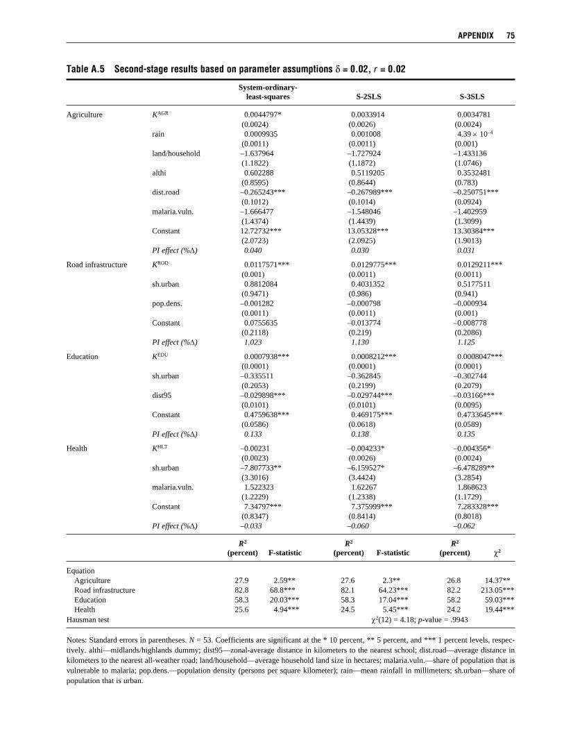
AppEndix 75
Table A.5 Second-stage results based on parameter assumptions d = 0.02, r = 0.02
System-ordinary- least-squares S-2SLS S-3SLS
Agriculture KAGR 0.0044797* 0.0033914 0.0034781 (0.0024) (0.0026) (0.0024) rain 0.0009935 0.001008 4.39 × 10⁻⁴
(0.0011) (0.0011) (0.001) land/household –1.637964 –1.727924 –1.433136 (1.1822) (1.1872) (1.0746) althi 0.602288 0.5119205 0.3532481 (0.8595) (0.8644) (0.783) dist.road –0.265243*** –0.267989*** –0.250751*** (0.1012) (0.1014) (0.0924) malaria.vuln. –1.666477 –1.548046 –1.402959 (1.4374) (1.4439) (1.3099) Constant 12.72732*** 13.05328*** 13.30384*** (2.0723) (2.0925) (1.9013) PI effect (%∆) 0.040 0.030 0.031
Road infrastructure KROD 0.0117571*** 0.0129775*** 0.0129211*** (0.001) (0.0011) (0.0011) sh.urban 0.8812084 0.4031352 0.5177511 (0.9471) (0.986) (0.941) pop.dens. –0.001282 –0.000798 –0.000934 (0.0011) (0.0011) (0.001) Constant 0.0755635 –0.013774 –0.008778 (0.2118) (0.219) (0.2086) PI effect (%∆) 1.023 1.130 1.125
Education KEDU 0.0007938*** 0.0008212*** 0.0008047*** (0.0001) (0.0001) (0.0001) sh.urban –0.335511 –0.362845 –0.302744 (0.2053) (0.2199) (0.2079) dist95 –0.029898*** –0.029744*** –0.03166*** (0.0101) (0.0101) (0.0095) Constant 0.4759638*** 0.469175*** 0.4733645*** (0.0586) (0.0618) (0.0589) PI effect (%∆) 0.133 0.138 0.135
Health KHLT –0.00231 –0.004233* –0.004356* (0.0023) (0.0026) (0.0024) sh.urban –7.807733** –6.159527* –6.478289** (3.3016) (3.4424) (3.2854) malaria.vuln. 1.522323 1.62267 1.868623 (1.2229) (1.2338) (1.1729) Constant 7.34797*** 7.375999*** 7.283328*** (0.8347) (0.8414) (0.8018) PI effect (%∆) –0.033 –0.060 –0.062
R2 R2 R2 (percent) F-statistic (percent) F-statistic (percent) c2
Equation Agriculture 27.9 2.59** 27.6 2.3** 26.8 14.37** Road infrastructure 82.8 68.8*** 82.1 64.23*** 82.2 213.05*** Education 58.3 20.03*** 58.3 17.04*** 58.2 59.03*** Health 25.6 4.94*** 24.5 5.45*** 24.2 19.44***Hausman test c2(12) = 4.18; p-value = .9943
Notes: Standard errors in parentheses. N = 53. Coefficients are significant at the * 10 percent, ** 5 percent, and *** 1 percent levels, respec-tively. althi—midlands/highlands dummy; dist95—zonal-average distance in kilometers to the nearest school; dist.road—average distance in kilometers to the nearest all-weather road; land/household—average household land size in hectares; malaria.vuln.—share of population that is vulnerable to malaria; pop.dens.—population density (persons per square kilometer); rain—mean rainfall in millimeters; sh.urban—share of population that is urban.
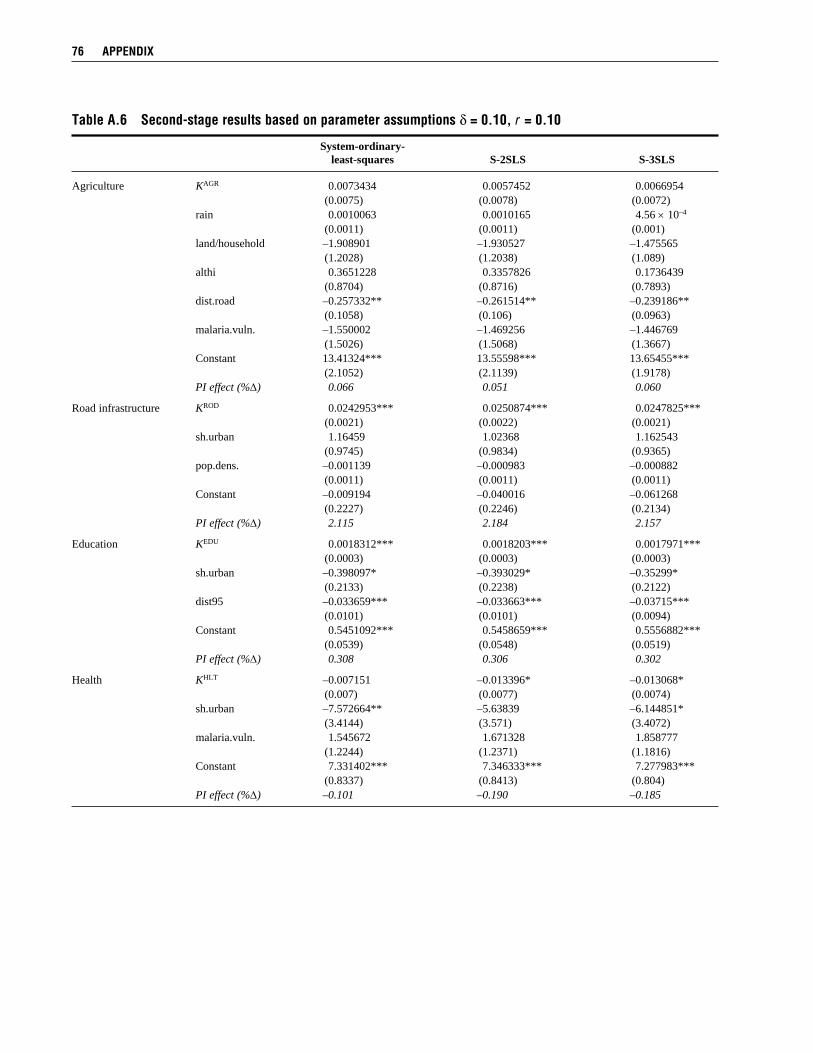
76 AppEndix
Table A.6 Second-stage results based on parameter assumptions d = 0.10, r = 0.10
System-ordinary- least-squares S-2SLS S-3SLS
Agriculture KAGR 0.0073434 0.0057452 0.0066954 (0.0075) (0.0078) (0.0072) rain 0.0010063 0.0010165 4.56 × 10⁻⁴
(0.0011) (0.0011) (0.001) land/household –1.908901 –1.930527 –1.475565 (1.2028) (1.2038) (1.089) althi 0.3651228 0.3357826 0.1736439 (0.8704) (0.8716) (0.7893) dist.road –0.257332** –0.261514** –0.239186** (0.1058) (0.106) (0.0963) malaria.vuln. –1.550002 –1.469256 –1.446769 (1.5026) (1.5068) (1.3667) Constant 13.41324*** 13.55598*** 13.65455*** (2.1052) (2.1139) (1.9178) PI effect (%∆) 0.066 0.051 0.060
Road infrastructure KROD 0.0242953*** 0.0250874*** 0.0247825*** (0.0021) (0.0022) (0.0021) sh.urban 1.16459 1.02368 1.162543 (0.9745) (0.9834) (0.9365) pop.dens. –0.001139 –0.000983 –0.000882 (0.0011) (0.0011) (0.0011) Constant –0.009194 –0.040016 –0.061268 (0.2227) (0.2246) (0.2134) PI effect (%∆) 2.115 2.184 2.157
Education KEDU 0.0018312*** 0.0018203*** 0.0017971*** (0.0003) (0.0003) (0.0003) sh.urban –0.398097* –0.393029* –0.35299* (0.2133) (0.2238) (0.2122) dist95 –0.033659*** –0.033663*** –0.03715*** (0.0101) (0.0101) (0.0094) Constant 0.5451092*** 0.5458659*** 0.5556882*** (0.0539) (0.0548) (0.0519) PI effect (%∆) 0.308 0.306 0.302
Health KHLT –0.007151 –0.013396* –0.013068* (0.007) (0.0077) (0.0074) sh.urban –7.572664** –5.63839 –6.144851* (3.4144) (3.571) (3.4072) malaria.vuln. 1.545672 1.671328 1.858777 (1.2244) (1.2371) (1.1816) Constant 7.331402*** 7.346333*** 7.277983*** (0.8337) (0.8413) (0.804) PI effect (%∆) –0.101 –0.190 –0.185

AppEndix 77
Table A.7 Second-stage results based on parameter assumptions d = 0.02, r = 0.10
System-ordinary- least-squares S-2SLS S-3SLS
Agriculture KAGR 0.0063388 0.0049654 0.0053344 (0.0046) (0.0047) (0.0044) rain 0.000978 0.0009943 4.12 × 10⁻⁴
(0.0011) (0.0011) (0.0010) land/household –1.783875 –1.832495 –1.436365 (1.1957) (1.1977) (1.0829) althi 0.4605443 0.4106586 0.2486524 (0.8655) (0.8675) (0.7850) dist.road –0.256326** –0.260707** –0.238641** (0.1037) (0.1039) (0.0945) malaria.vuln. –1.645407 –1.544346 –1.462392 (1.4757) (1.4799) (1.3417) Constant 13.08958*** 13.30181*** 13.46663*** (2.0948) (2.1051) (1.9099) PI effect (%∆) 0.057 0.044 0.048
Road infrastructure KROD 0.0183379*** 0.0192091*** 0.0190418*** (0.0016) (0.0017) (0.0016) sh.urban 1.047392 0.8364875 0.9771267 (0.9523) (0.9661) (0.9210) pop.dens. –0.001116 –0.000887 –0.000887 (0.0011) (0.0011) (0.0010) Constant –0.04497 –0.091583 –0.103041 (0.2179) (0.2209) (0.2104) PI effect (%∆) 1.596 1.672 1.658
Education KEDU 0.001292*** 0.0013044*** 0.0012737*** (0.0002) (0.0002) (0.0002) sh.urban –0.390548* –0.398687* –0.34193 (0.2099) (0.2221) (0.2104) dist95 –0.031873*** –0.031849*** –0.034501*** (0.0100) (0.0100) (0.0094)
(continued )
Table A.6 Continued
System-ordinary- least-squares S-2SLS S-3SLS
R2 R2 R2 (percent) F-statistic (percent) F-statistic (percent) c2
Equation Agriculture 23.7 2.07* 23.6 2.00* 22.8 11.92* Road infrastructure 81.4 62.91*** 81.4 61.43*** 81.4 198.84*** Education 57.8 19.65*** 57.8 17.07*** 57.7 60.68*** Health 25.7 4.96*** 24.4 5.54*** 24.4 19.3***Hausman test c2(12) = 3.81; p-value = .9983
Notes: Standard errors in parentheses. N = 53. Coefficients are significant at the * 10 percent, ** 5 percent, and *** 1 percent levels, respec-tively. althi—midlands/highlands dummy; dist95—zonal-average distance in kilometers to the nearest school; dist.road—average distance in kilometers to the nearest all-weather road; land/household—average household land size in hectares; malaria.vuln.—share of population that is vulnerable to malaria; pop.dens.—population density (persons per square kilometer); rain—mean rainfall in millimeters; sh.urban—share of population that is urban.

78 AppEndix
Table A.8 Second-stage results based on parameter assumptions d = 0.10, r = 0.02
System-ordinary- least-squares S-2SLS S-3SLS
Agriculture KAGR 0.0077097 0.0059015 0.0066208 (0.0066) (0.0068) (0.0063) rain 0.0010027 0.0010146 4.52 × 10⁻⁴
(0.0011) (0.0011) (0.0010) land/household –1.863791 –1.897678 –1.464665 (1.1989) (1.2005) (1.0860) althi 0.4115358 0.3690294 0.2089996 (0.8690) (0.8708) (0.7885) dist.road –0.25694** –0.261539** –0.240368** (0.1048) (0.1049) (0.0954) malaria.vuln. –1.598452 –1.500066 –1.455414 (1.4903) (1.4947) (1.3557) Constant 13.25734*** 13.44773*** 13.56946*** (2.1032) (2.1132) (1.9177) PI effect (%∆) 0.069 0.053 0.059
(continued )
Table A.7 Continued
System-ordinary- least-squares S-2SLS S-3SLS
Constant 0.5111955*** 0.5096438*** 0.5174259*** (0.0556) (0.0573) (0.0545) PI effect (%∆) 0.217 0.219 0.214
Health KHLT –0.004304 –0.00787* –0.007886* (0.0043) (0.0047) (0.0044) sh.urban –7.667972** –5.911767* –6.33169* (3.3647) (3.505) (3.3445) malaria.vuln. 1.536393 1.647922 1.843428 (1.2237) (1.2349) (1.1793) Constant 7.339579*** 7.360521*** 7.295791*** (0.834) (0.8409) (0.8035) PI effect (%∆) –0.061 –0.111 –0.112
R2 R2 R2 (percent) F-statistic (percent) F-statistic (percent) c2
Equation Agriculture 25.5 2.28** 25.3 2.14* 24.5 12.88** Road infrastructure 82.4 67.01*** 82.3 64.89*** 82.3 211.99*** Education 58.5 20.24*** 58.5 17.45*** 58.4 60.41*** Health 25.7 4.96*** 24.5 5.50*** 24.4 19.40***Hausman test c2(12) = 3.64; p-value = .9973
Notes: Standard errors in parentheses. N = 53. Coefficients are significant at the * 10 percent, ** 5 percent, and *** 1 percent levels, respec-tively. althi—midlands/highlands dummy; dist95—zonal-average distance in kilometers to the nearest school; dist.road—average distance in kilometers to the nearest all-weather road; land/household—average household land size in hectares; malaria.vuln.—share of population that is vulnerable to malaria; pop.dens.—population density (persons per square kilometer); rain—mean rainfall in millimeters; sh.urban—share of population that is urban.

AppEndix 79
Table A.8 Continued
System-ordinary- least-squares S-2SLS S-3SLS
Road infrastructure KROD 0.0227498*** 0.0235789*** 0.0233372*** (0.0019) (0.0020) (0.0020) sh.urban 1.064426 0.9032573 1.037949 (0.9535) (0.9642) (0.9186) pop.dens. –0.001111 –0.000935 –0.000874 (0.0011) (0.0011) (0.0010) Constant 0.0015711 –0.032491 –0.049865 (0.2168) (0.2189) (0.2082) PI effect (%∆) 1.980 2.05 2.031
Education KEDU 0.0016877*** 0.0016794*** 0.0016468*** (0.0003) (0.0003) (0.0003) sh.urban –0.394779* –0.390597* –0.342232 (0.2113) (0.2224) (0.2108) dist95 –0.033027*** –0.033033*** –0.036275*** (0.0101) (0.0101) (0.0094) Constant 0.5322592*** 0.5329491*** 0.5425204*** (0.0544) (0.0556) (0.0527) PI effect (%∆) 0.284 0.282 0.277
Health KHLT –0.006192 –0.011518* –0.011378* (0.0061) (0.0067) (0.0064) sh.urban –7.620974** –5.7575 –6.219435* (3.3907) (3.5435) (3.3814) malaria.vuln. 1.540637 1.660062 1.856967 (1.2241) (1.2362) (1.1807) Constant 7.335046*** 7.352886*** 7.282146*** (0.8339) (0.8412) (0.8039) PI effect (%∆) –0.088 –0.163 –0.161
R2 R2 R2 (percent) F-statistic (percent) F-statistic (percent) c2
Equation Agriculture 24.5 2.16** 24.3 2.05* 23.6 12.34* Road infrastructure 82.3 66.73*** 82.2 64.72*** 82.3 210.42*** Education 58.3 20.03*** 58.3 17.23*** 58.1 60.57*** Health 25.7 4.96*** 24.4 5.52*** 24.4 19.34***Hausman test c2(12) = 3.84; p-value = .9982
Notes: Standard errors in parentheses. N = 53. Coefficients are significant at the * 10 percent, ** 5 percent, and *** 1 percent levels, respec-tively. althi—midlands/highlands dummy; dist95—zonal-average distance in kilometers to the nearest school; dist.road—average distance in kilometers to the nearest all-weather road; land/household—average household land size in hectares; malaria.vuln.—share of population that is vulnerable to malaria; pop.dens.—population density (persons per square kilometer); rain—mean rainfall in millimeters; sh.urban—share of population that is urban.
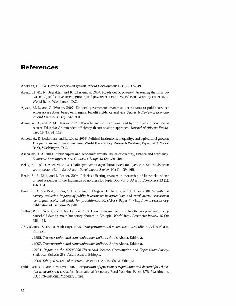
References
Adelman, I. 1984. Beyond export-led growth. World Development 12 (9): 937–949.
Agenor, P.-R., N. Bayraktar, and K. El Aynaoui. 2004. Roads out of poverty? Assessing the links be-tween aid, public investment, growth, and poverty reduction. World Bank Working Paper 3490. World Bank, Washington, D.C.
Ajwad, M. I., and Q. Wodon. 2007. Do local governments maximise access rates to public services across areas? A test based on marginal benefit incidence analysis. Quarterly Review of Econom-ics and Finance 47 (2): 242–260.
Alene, A. D., and R. M. Hassan. 2005. The efficiency of traditional and hybrid maize production in eastern Ethiopia: An extended efficiency decomposition approach. Journal of African Econo-mies 15 (1): 91–116.
Allcott, H., D. Lederman, and R. López. 2006. Political institutions, inequality, and agricultural growth: The public expenditure connection. World Bank Policy Research Working Paper 3902. World Bank, Washington, D.C.
Aschauer, D. A. 2000. Public capital and economic growth: Issues of quantity, finance and efficiency. Economic Development and Cultural Change 48 (2): 391–406.
Belay, K., and D. Abebaw. 2004. Challenges facing agricultural extension agents: A case study from south-western Ethiopia. African Development Review 16 (1): 139–168.
Benin, S., S. Ehui, and J. Pender. 2004. Policies affecting changes in ownership of livestock and use of feed resources in the highlands of northern Ethiopia. Journal of African Economies 13 (1): 166–194.
Benin, S., A. Nin Pratt, S. Fan, C. Breisinger, T. Mogues, J. Thurlow, and X. Diao. 2008. Growth and poverty reduction impacts of public investments in agriculture and rural areas: Assessment techniques, tools, and guide for practitioners. ReSAKSS Paper 7. <http://www.resakss.org/publications/DiscussionP7.pdf>.
Collier, P., S. Dercon, and J. Mackinnon. 2002. Density versus quality in health care provision: Using household data to make budgetary choices in Ethiopia. World Bank Economic Review 16 (3): 425–448.
CSA (Central Statistical Authority). 1995. Transportation and communications bulletin. Addis Ababa, Ethiopia.
———. 1996. Transportation and communications bulletin. Addis Ababa, Ethiopia.
———. 1997. Transportation and communications bulletin. Addis Ababa, Ethiopia.
———. 2001. Report on the 1999/2000 Household Income, Consumption and Expenditure Survey. Statistical Bulletin 258. Addis Ababa, Ethiopia.
———. 2004. Ethiopia statistical abstract. December. Addis Ababa, Ethiopia.
Dabla-Norris, E., and J. Matovu. 2002. Composition of government expenditure and demand for educa-tion in developing countries. International Monetary Fund Working Paper 2/78. Washington, D.C.: International Monetary Fund.
80
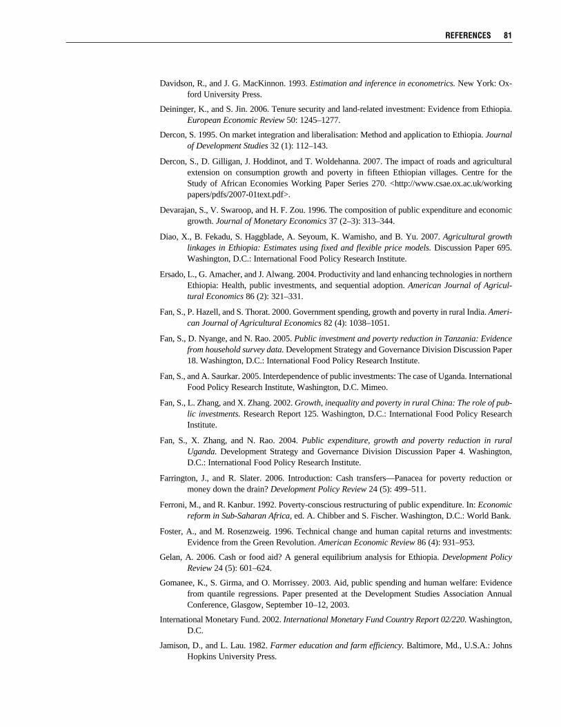
Davidson, R., and J. G. MacKinnon. 1993. Estimation and inference in econometrics. New York: Ox-ford University Press.
Deininger, K., and S. Jin. 2006. Tenure security and land-related investment: Evidence from Ethiopia. European Economic Review 50: 1245–1277.
Dercon, S. 1995. On market integration and liberalisation: Method and application to Ethiopia. Journal of Development Studies 32 (1): 112–143.
Dercon, S., D. Gilligan, J. Hoddinot, and T. Woldehanna. 2007. The impact of roads and agricultural extension on consumption growth and poverty in fifteen Ethiopian villages. Centre for the Study of African Economies Working Paper Series 270. <http://www.csae.ox.ac.uk/working papers/pdfs/2007-01text.pdf>.
Devarajan, S., V. Swaroop, and H. F. Zou. 1996. The composition of public expenditure and economic growth. Journal of Monetary Economics 37 (2–3): 313–344.
Diao, X., B. Fekadu, S. Haggblade, A. Seyoum, K. Wamisho, and B. Yu. 2007. Agricultural growth linkages in Ethiopia: Estimates using fixed and flexible price models. Discussion Paper 695. Washington, D.C.: International Food Policy Research Institute.
Ersado, L., G. Amacher, and J. Alwang. 2004. Productivity and land enhancing technologies in northern Ethiopia: Health, public investments, and sequential adoption. American Journal of Agricul-tural Economics 86 (2): 321–331.
Fan, S., P. Hazell, and S. Thorat. 2000. Government spending, growth and poverty in rural India. Ameri-can Journal of Agricultural Economics 82 (4): 1038–1051.
Fan, S., D. Nyange, and N. Rao. 2005. Public investment and poverty reduction in Tanzania: Evidence from household survey data. Development Strategy and Governance Division Discussion Paper 18. Washington, D.C.: International Food Policy Research Institute.
Fan, S., and A. Saurkar. 2005. Interdependence of public investments: The case of Uganda. International Food Policy Research Institute, Washington, D.C. Mimeo.
Fan, S., L. Zhang, and X. Zhang. 2002. Growth, inequality and poverty in rural China: The role of pub-lic investments. Research Report 125. Washington, D.C.: International Food Policy Research Institute.
Fan, S., X. Zhang, and N. Rao. 2004. Public expenditure, growth and poverty reduction in rural Uganda. Development Strategy and Governance Division Discussion Paper 4. Washington, D.C.: International Food Policy Research Institute.
Farrington, J., and R. Slater. 2006. Introduction: Cash transfers—Panacea for poverty reduction or money down the drain? Development Policy Review 24 (5): 499–511.
Ferroni, M., and R. Kanbur. 1992. Poverty-conscious restructuring of public expenditure. In: Economic reform in Sub-Saharan Africa, ed. A. Chibber and S. Fischer. Washington, D.C.: World Bank.
Foster, A., and M. Rosenzweig. 1996. Technical change and human capital returns and investments: Evidence from the Green Revolution. American Economic Review 86 (4): 931–953.
Gelan, A. 2006. Cash or food aid? A general equilibrium analysis for Ethiopia. Development Policy Review 24 (5): 601–624.
Gomanee, K., S. Girma, and O. Morrissey. 2003. Aid, public spending and human welfare: Evidence from quantile regressions. Paper presented at the Development Studies Association Annual Conference, Glasgow, September 10–12, 2003.
International Monetary Fund. 2002. International Monetary Fund Country Report 02/220. Washington, D.C.
Jamison, D., and L. Lau. 1982. Farmer education and farm efficiency. Baltimore, Md., U.S.A.: Johns Hopkins University Press.
references 81

Jayne, T. S., J. Govereh, A. Mwanaumo, and J. K. Nyoro. 2002. False promise or false premise? The experience of food and input market reform in eastern and southern Africa. World Development 30 (11): 1967–1985.
Jung, H.-S., and E. Thorbecke. 2003. The impact of public education expenditure on human capital, growth, and poverty in Tanzania and Zambia: A general equilibrium approach. Journal of Policy Modelling 25 (8): 701–725.
Kloos, H. 1998. Primary health care in Ethiopia under three political systems: Community participation in a war-torn society. Social Science and Medicine 46 (4): 505–522.
Lofgren, H., and S. Robinson. 2005. Public spending, growth and poverty alleviation in Sub-Saharan Africa: A dynamic general equilibrium analysis. Paper prepared for the conference at the Centre for the Study of African Economies, March 21–22, 2004.
López, R., and G. Galinato. 2007. Should governments stop subsidies to private goods? Evidence from rural Latin America. Journal of Public Economics 91: 1071–1094.
López, R., and A. Islam. 2008. The structure of government expenditures and economic growth in a context of market failure. Working paper, University of Maryland–College Park.
Ministry of Education. Various years. Education statistics annual abstract. Education Management Information Systems. Addis Ababa, Ethiopia.
Ministry of Health. Various years. Health and health-related indicators. Planning and Programming De-partment, Health Information Processing and Documentation Team. Addis Ababa, Ethiopia.
MOFED (Ministry of Finance and Economic Development). Various years. Countrywide budgetary revenue and expenditure. Addis Ababa, Ethiopia.
———. 2002. Ethiopia: Sustainable Development and Poverty Reduction Programme. Ministry of Finance and Economic Development. Addis Ababa, Ethiopia.
MOPED. 1993. An economic development strategy for Ethiopia: A comprehensive guide and a devel-opment strategy for the future. Ministry of Planning and Economic Development. September. Addis Ababa, Ethiopia.
Paternostro, S., A. Rajaram, and E. R. Tiongson. 2007. How does the composition of public spending matter? Oxford Development Studies 35 (1): 47–82.
Pausewang, S., K. Tronvoll, and L. Aalen. 2002. Ethiopia since the Derg: A decade of democratic pre-tension and performance. London: Zed.
Roseboom, J. 2002. Underinvestment in agricultural R&D revisited. Quarterly Journal of International Agriculture 41 (4): 297–316.
Russell, S., and K. Abdella. 2002. Too poor to be sick: Coping with the costs of illness in East Hararghe, Ethiopia. London: Save the Children.
Seifu, M. 2002. Benefit incidence analysis on public sector expenditures in Ethiopia: The case of educa-tion and health. Paper submitted to the Annual Conference on the Ethiopian Economy.
Teferra, M. 2002. Power sector reforms in Ethiopia: Options for promoting local investments in rural electrification. Energy Policy 30: 967–975.
Van de Walle, D. 2000. Are returns to investment lower for the poor? Human and physical capital interactions in rural Vietnam. World Bank Policy Research Working Paper 2425. World Bank, Washington, D.C.
Wolde-Ghiorgis, W. 2002. Renewable energy for rural development in Ethiopia: The case for new energy policies and institutional reform. Energy Policy 30: 1095–1105.
World Bank. 2002. Ethiopia—Financing public expenditures for poverty reduction: Public expenditure review. Washington, D.C.
———. 2003. Ethiopia country financial accountability assessment. Washington, D.C.
82 references

———. 2004. Ethiopia—Public expenditure review: The emerging challenge. Washington, D.C.
———. 2005a. Education in Ethiopia: Strengthening the foundation for sustainable progress. World Bank Country Study. Washington, D.C.
———. 2005b. A strategy to stimulate and balance growth in Ethiopia. World Bank Country Economic Memorandum. Washington, D.C.
———. 2005c. Ethiopia: A country status report on health and poverty. Report 28963-ET. Washington, D.C.
———. 2005d. Well-being and poverty in Ethiopia: The role of agriculture and agency. Report 29468-ET. Washington, D.C.
———. 2005e. World development indicators. Washington, D.C.
———. 2007. World development indicators. Washington, D.C.
———. 2008. Ethiopia: Agriculture and rural development public expenditure review 1997/98– 2005/06. Report 41902-ET. Washington, D.C.
references 83