Embed Size (px)
Citation preview

Public sector productivity
Quality adjusting sector-level data on New Zealand schools
Working Paper 2017/2
May 2017
Authors: Norman Gemmell, Patrick Nolan and Grant Scobie
Public sector productivity: Quality adjusting sector-level data on New Zealand schools
ii
How to cite this document: Gemmell, N., Nolan, P. & Scobie, G. (2017). Public sector
productivity: Quality adjusting sector-level data on New Zealand schools. New Zealand
Productivity Commission Working Paper 2017/2
Date: May 2017
JEL classifications: D24, H41, H52, I21, O4
ISBN: 978-0-478-44038-6 (online only)
Acknowledgements:
Special acknowledgement is due to Guanyu Zheng at the New Zealand Productivity
Commission for econometric analyses of the relationship between income and qualifications.
Matthew Horwell was a Victoria University of Wellington summer scholar at the Commission in
2015-16 and did valuable work on quality adjustment. Thanks also to Murray Sherwin, Graham
Scott, Sally Davenport, Dave Heatley, Amy Russell, Paul Conway, Geoff Lewis, Lisa Meehan,
Simon Wakeman and other colleagues at the Commission for their comments on drafts of this
work.
Warren Smart at the Ministry of Education responded patiently to repeated request for data.
Thanks also to David Earle, Nik Green, Jasmine Ludwig, Cyril Mako, Shona Ramsay, Philip
Stevens, and John Wardrop at the Ministry of Education. At Statistics New Zealand Paul Pascoe,
Adam Tipper, Daniel Griffiths, Gary Dunnet, Cameron Adams, David Lum, Dean Edwards, Ewan
Jonasen and Evelyn Ocansey provided considerable help in accessing data and explanations of
the system of national accounts.
Thanks also to John Daley, Jim Minifie, Peter Goss and Jordana Hunter at the Grattan Institute;
Jenny Gordon, Patrick Jomani, Anna Heaney, Greg Murgouth, John Salarian, and Ralph
Lattimore at the Australian Productivity Commission; Derek Burnell, Katherine Keenan, Stephen
Howe, David Stewart, Peter Williams, Ben Loughton, Ian Ewing, Hui Wei, David Hansell, Jason
Annabel, Shiji Zhao and Jennifer Humphrys at the Australian Bureau of Statistics; Paul Rouse and
Dimitri Margaritis, University of Auckland; Trinh Le, Motu; Bryce Wilkinson, New Zealand
Initiative; Eric Hanushek, Stanford Institute; and Jason Gush at the Royal Society of New
Zealand.
Disclaimer:
The views expressed in this Working Paper are strictly those of the authors. They do not
necessarily reflect the views of the New Zealand Productivity Commission or the New
Zealand Government. The authors are solely responsible for any errors or omissions.
The contents of this report must not be construed as legal advice. The Commission does
not accept any responsibility or liability for an action taken as a result of reading, or reliance
placed because of having read any part, or all, of the information in this report. The
Working paper 2017/02
iii
The New Zealand Productivity Commission (Te Kōmihana Whai Hua o Aotearoa1) – an
independent Crown Entity – completes in-depth inquiry reports on topics selected by the
Government, carries out productivity-related research, and promotes understanding of
productivity issues. The Commission’s work is guided by the New Zealand Productivity
Commission Act 2010.
Information on the Commission can be found on www.productivity.govt.nz or by calling +64 4 903 5150.
1 The Commission that pursues abundance for New Zealand.
Commission does not accept any responsibility or liability for any error, inadequacy,
deficiency, flaw in or omission from this report.
Access to data used in this paper was provided by Statistics New Zealand in accordance
with security and confidentiality provisions of the Statistics Act 1975. The results presented
in this study are the work of the authors, not Statistics New Zealand.
Public sector productivity: Quality adjusting sector-level data on New Zealand schools
iv
Contents
1 Executive summary .............................................................................................. 6
2 Key concepts ...................................................................................................... 11 2.1 What is productivity? .............................................................................................. 11 2.2 Challenges in applying productivity concepts to public services ....................... 12 2.3 Productivity and public sector performance metrics ........................................... 18
3 The existing picture ............................................................................................ 20 3.1 The Statistics New Zealand approach ................................................................... 20 3.2 Aggregate labour productivity .............................................................................. 21 3.3 Trends for particular public services ...................................................................... 24 3.4 What other studies tell us ...................................................................................... 25 3.5 Quality adjustments ................................................................................................ 26 3.6 Quality adjustments in this paper .......................................................................... 31
4 School productivity ............................................................................................ 34 4.1 Basic measures........................................................................................................ 34 4.2 Adjusting labour input for composition ................................................................ 38 4.3 Adjusting output for pupil attainment .................................................................. 39 4.4 Adjusting for outcomes (earnings) ........................................................................ 42 4.5 Bringing measures together .................................................................................. 45
5 Comparison with ONS estimates of education productivity ............................... 48
6 References ......................................................................................................... 51
Appendix A Summary of results with alternative deflator ................................... 61
Appendix B Additional data on real expected income by attainment level ......... 62
Appendix C Background on frontier approaches ................................................. 64
Tables
Table 1 Examples of quality adjustments for schools ....................................................... 7 Table 2 Average annual rates of growth in labour productivity: New Zealand and
Australia (1996-2014) ............................................................................................ 22 Table 3 Labour productivity growth rates before and after the Global Financial
Crisis ...................................................................................................................... 23 Table 4 Average annual rates of growth in labour productivity within the public sector
(1996-2015) ............................................................................................................ 24 Table 5 Key challenges in quality adjusting data on schools ......................................... 29 Table 6 Summary of measures used in this paper .......................................................... 32 Table 7 Basic input and output data for schools (1997-2015) ......................................... 34 Table 8 Summary of basic measures of productivity growth in the school sector ........ 38 Table 9 Student numbers over real salaries (2006 dollars) (2002-2014) (2002=1,000) ... 39
Working paper 2017/02
v
Table 10 Measures based on outcomes adjusted for PISA scores (2003-2015) (2003=1,000) ......................................................................................................... 40
Table 11 Measures based on outcomes adjusted for TIMMS scores (2002-2014) (2002=1,000) ......................................................................................................... 40
Table 12 Definitions of attainment categories for the New Zealand Income Survey ..... 43 Table 13 Student numbers in attainment categories (1997-2014) (1997=1,000) ............. 44 Table 14 Productivity indexes based on earnings adjusted school attainment (1997-
2014) (1997=1,000) ............................................................................................... 45 Table 15 Summary of measures (CPI deflator) .................................................................. 46 Table 16 Comparison with ONS estimates of education productivity (1997 to 2014)
(1997=1,000) ......................................................................................................... 49
Figures
Figure 1 Comparison with ONS estimates of education productivity (1997 to 2014) (1997=1,000) ......................................................................................................... 10
Figure 2 A national accounts perspective on productivity ............................................... 11 Figure 3 Dimensions of public sector performance ......................................................... 19 Figure 4 Total economy, measured sector and public sector labour productivity
indexes (1996-2014) (1996=1,000) ....................................................................... 23 Figure 5 Output inefficiency in secondary education (2009 and 2012) ........................... 25 Figure 6 School pupil-staff ratio and real revenue per pupil (2006 dollars) (1997-2015) 37 Figure 7 Comparison with ONS estimates of education productivity (1997 to 2014)
(1997=1,000) ......................................................................................................... 50
Public sector productivity: Quality adjusting sector-level data on New Zealand schools
6
1 Executive summary
Statistics New Zealand has estimated that since 1996 increases in outputs of the public sector
have largely been associated with increasing labour inputs. In the education sector, for example,
the average annual increase in output of 1.0% between 1996 and 2015 was composed of
average annual labour input growth of 2.5% while labour productivity fell on average by 1.5%
per annum. These data use standard aggregate productivity methods and are not part of the
National Accounts.2 They involve no explicit quality adjustment. This is important as it is difficult
to fully understand productivity data (especially trends over time) without considering the
impact of changes in quality.
Yet while important in principle adjusting public sector productivity data for quality changes is
complex in practice. As an example, the United Kingdom Office for National Statistics (ONS) has
had to revise its approach to quality adjusting education quantity when practices regarding
students sitting exams changed.3 This paper thus estimates a range of quality adjusted
productivity measures and discusses the benefits and risks of different approaches (e.g.,
regarding teacher salaries, students’ performance in tests, or impact on earnings). The measures
are illustrated with data on schools.
Why education?
A focus on the productivity of the education sector is consistent with a desire to help upskill the
economy (Atkinson, 2005) and the Better Public Services programme.4 This is also a topic of
interest to researchers concerned with productivity measurement more generally given the
variety of messages that emerge for this sector from different approaches to productivity
analysis. While national accounts data show declining labour productivity in the education
sector as a whole a number of cross country studies (largely focussing on schools) have
suggested that the New Zealand education system performs relatively well internationally (e.g.,
Afonso and Aubyn, 2005; Sutherland et al., 2007; and Schreyer, 2010). More recent work (Dutu
and Sicari, 2016), has however, suggested that New Zealand may have fallen back to the middle
of the pack.
This investigation on quality adjustment and school productivity could thus help with
interpretation of any evidence of a lagging productivity performance in the public sector,
2 As discussed in 3.1, these data are based on the industry classification of output and so include a mixture of organisations in public and private
ownership. These figures also include outputs which are traded for economically significant prices (e.g., in markets). Public sector industries
(education and training, health and social care, central government administration and local government administration), along with owner
occupied housing, make up what Statistics New Zealand refer to as the non-measured sector. Based on a production measure of GDP public
sector output as percentage of total industry output was 15.8% in 2015.
3 This is significant as any quality adjustment makes a substantial difference to measured productivity. From 1997 to 2011, quality-adjusted
output growth in the United Kingdom education sector grew at an annual average rate of 2.7%. Of this the quality adjustment accounted for
90%, or an annual rate of growth of 2.5% (Caul, 2014, p. 8).
4 This programme set out ten specific challenges for the public sector to achieve over a five year period to 2018. Two of these relate to
education and are aimed at boosting skills and employment. The targets are: 85% of 18-year-olds will have NCEA Level 2 or an equivalent
qualification by 2017; 60% of 25-34 year olds will have achieved qualifications at NZQF Level 4 and above by 2018.

Working paper 2017/02
7
including whether this tells us something about the public services themselves or more about
the measures being used.
So what difference could quality adjustment make?
Estimates of labour and multifactor productivity including quality adjustments for New Zealand
schools were developed using data at the sector-level (the measures and key results are
summarised in Table 1). To illustrate the potential of existing data – and also to allow these
measures to be replicated – emphasis was given to using data from publicly available sources.
Table 1 Examples of quality adjustments for schools
Measure Formal
equivalent
Data Results
Basic labour productivity (Total Student Places / Teacher FTEs)
Q/L Total student places based on data for student roll by school type. Excludes students in private schools. FTE teachers (headcount for 2001 and earlier) in state and state integrated schools based on education counts data. Teaching staff includes principal, management, teacher, resource teachers, community education, guidance and therapists
Declined by 1.0% on average between 2002 and 2014, with the fastest decline between 2002 and 2008
Basic multifactor productivity (Total Student Places / School Revenue)
Q/(wL+rK+mM) Total student places as above. School revenue based on Core Crown Expenditure from Treasury Budget documents and percentage of non-government revenue from Ministry of Education. Core Crown Expenditure covers roll-based operations funding to schools, teacher and management salaries, support costs and supplementary funding programmes. Indexation is based on the full CPI
Declined by 1.7% on average between 2002 and 2014, also with the fastest decline between 2002 and 2008
Labour productivity based on adjusted labour input (Total Student Places / Teacher Salaries)
Q/wL Total student places as above. Expenditure on teacher salaries (primary and secondary) in state and state integrated schools from education counts. Indexation is based on the full CPI
Declined by an average of 2.0% between 2002 and 2014, although grew by an average of 0.2% between 2008-2014
Labour productivity based on adjusted output (pupil attainment) (Aggregate PISA Points / Teacher FTEs)
pQ/L Total student places (primary and secondary) weighted by attainment in unweighted averages of the reading, mathematics and science PISA scores. Primary and secondary teacher FTEs
1.1% average decline between 2003 and 2015 (if using only secondary students and FTE teachers the decline was 1.0%)
Labour productivity based on adjusted output (pupil attainment) (Students Achieving Domestic Standard / Teacher FTEs)
pQ/L Total student places (primary and secondary) weighted by share of students leaving school with NCEA level 2 (or equivalent) or more. Primary and secondary teacher FTEs
0.8% average increase between 2002 and 2014
Multifactor productivity based on adjusted output
pQ/(wL+rK+mM) Total student places (primary and secondary) weighted by share of students leaving school
0.5% average decrease between
Public sector productivity: Quality adjusting sector-level data on New Zealand schools
8
Measure Formal
equivalent
Data Results
(pupil attainment) (Students Achieving Domestic Standard / School Revenue)
with NCEA level 2 (or equivalent) or more. School revenue based on Core Crown Expenditure from Treasury Budget documents and percentage of non-government revenue from Ministry of Education. Core Crown Expenditure covers roll-based operations funding to schools, teacher and management salaries, support costs and supplementary funding programmes. Indexation is based on the full CPI
2002 and 2014. This series is most directly comparable to the quality adjusted series used by the ONS
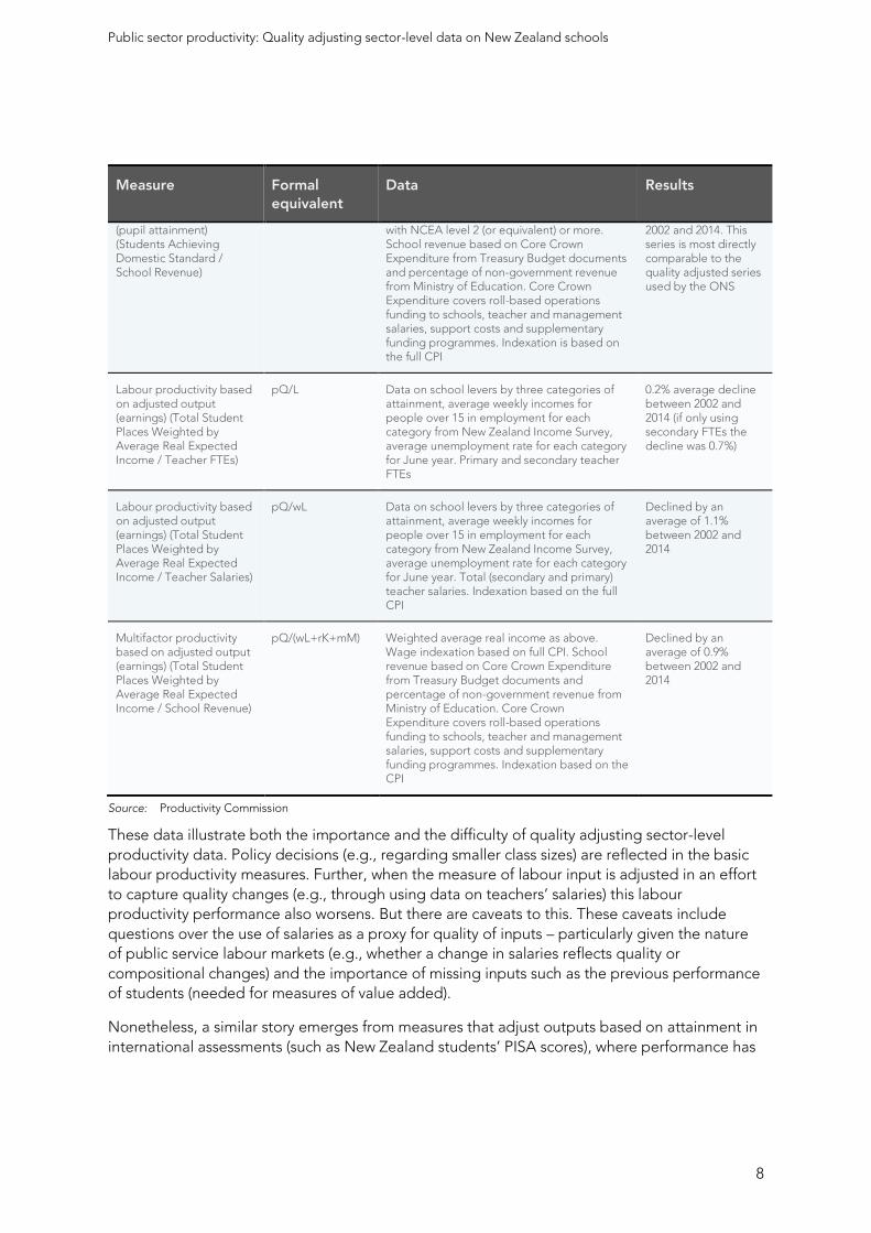
Labour productivity based on adjusted output (earnings) (Total Student Places Weighted by Average Real Expected Income / Teacher FTEs)
pQ/L Data on school levers by three categories of attainment, average weekly incomes for people over 15 in employment for each category from New Zealand Income Survey, average unemployment rate for each category for June year. Primary and secondary teacher FTEs
0.2% average decline between 2002 and 2014 (if only using secondary FTEs the decline was 0.7%)
Labour productivity based on adjusted output (earnings) (Total Student Places Weighted by Average Real Expected Income / Teacher Salaries)
pQ/wL Data on school levers by three categories of attainment, average weekly incomes for people over 15 in employment for each category from New Zealand Income Survey, average unemployment rate for each category for June year. Total (secondary and primary) teacher salaries. Indexation based on the full CPI
Declined by an average of 1.1% between 2002 and 2014
Multifactor productivity based on adjusted output (earnings) (Total Student Places Weighted by Average Real Expected Income / School Revenue)
pQ/(wL+rK+mM) Weighted average real income as above. Wage indexation based on full CPI. School revenue based on Core Crown Expenditure from Treasury Budget documents and percentage of non-government revenue from Ministry of Education. Core Crown Expenditure covers roll-based operations funding to schools, teacher and management salaries, support costs and supplementary funding programmes. Indexation based on the CPI
Declined by an average of 0.9% between 2002 and 2014
Source: Productivity Commission
These data illustrate both the importance and the difficulty of quality adjusting sector-level
productivity data. Policy decisions (e.g., regarding smaller class sizes) are reflected in the basic
labour productivity measures. Further, when the measure of labour input is adjusted in an effort
to capture quality changes (e.g., through using data on teachers’ salaries) this labour
productivity performance also worsens. But there are caveats to this. These caveats include
questions over the use of salaries as a proxy for quality of inputs – particularly given the nature
of public service labour markets (e.g., whether a change in salaries reflects quality or
compositional changes) and the importance of missing inputs such as the previous performance
of students (needed for measures of value added).
Nonetheless, a similar story emerges from measures that adjust outputs based on attainment in
international assessments (such as New Zealand students’ PISA scores), where performance has

Working paper 2017/02
9
worsened. This reflects a decline in aggregate PISA points (an average annual decline of 0.1%),
which itself reflects a larger fall in the average PISA score (an average annual decline of 0.3%).
However, there are differences in measured attainment according to international and domestic
assessments. Indeed, (labour) productivity based on a measure that adjusted for domestic
attainment (e.g., the proportion of students leaving school with at least NCEA level 2 (or
equivalent)) increased between 2002 and 2014. A related measure (the series using school
revenue as a measure of inputs) was used to compare the results in this paper to those of the
Office for National Statistics (ONS) in the United Kingdom (see below).
Finally, measures were adjusted for final outcomes (in this case the performance of school
leavers in the labour market). This involved a two-step process:
First, output was adjusted for the domestic attainment of students.
The average real expected income for students based on this attainment was then
estimated and multiplied by the number of students in each category.
These measures also suggested falling productivity. But these measures can be subject to
attribution problems. Indeed, given the improved domestic attainment above, the decline in
these measures reflects changes in unemployment and real wage growth following the Global
Financial Crisis. With the use of sector-level data it is thus not possible to conclude that changes
in these measures are directly attributable to the performance of schools, e.g., they may also
reflect differences in the economic context facing different cohorts of school leavers. To
estimate the incremental value of school education on earnings it would be necessary to use
linked unit record data.
Comparison with ONS estimates of education productivity
One series of results for schools in this paper is benchmarked against a series produced by the
ONS in the United Kingdom (Figure 1). In the United Kingdom output is based on the numbers
of students adjusted for absences. This is quality adjusted for the Level 2 attainment by students
in England, a five year geometric average of average point scores for students at this level in
Scotland, and average point scores for GCSEs in Wales. Student numbers are adjusted based
on the average point scores in these exams. As discussed in footnote 3, the ONS has had to
revise its approach to quality adjusting education quantity when practices regarding students
sitting exams changed.
In New Zealand output (numbers of primary and secondary students, not accounting for
absences) is adjusted based on the proportion of students completing schooling with NCEA
level 2 (or earlier equivalent) or more. In relation to input measures, in New Zealand school
revenue is used as the input measure. In the United Kingdom, inputs include labour, goods and
services, and consumption of fixed capital, which are all weighted by expenditure share.
It is important to recognise that given differences in public policies, policy contexts, and data
availability it is appropriate for there to be some small methodological differences in the two
approaches. Findings can thus be expected to differ. Yet similarities in the general magnitude
and direction of effect from making broadly similar quality adjustment (based on performance in
domestic assessments) can be expected.
Public sector productivity: Quality adjusting sector-level data on New Zealand schools
10
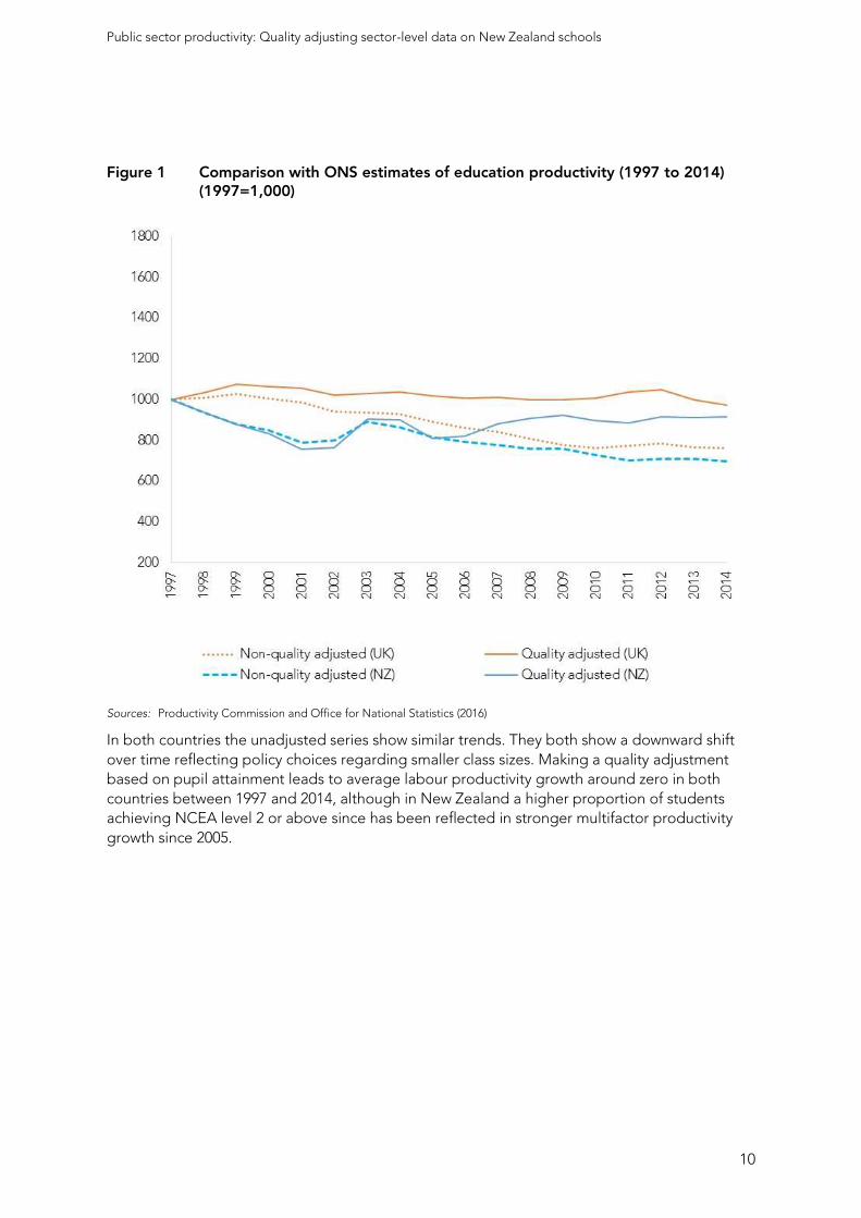
Figure 1 Comparison with ONS estimates of education productivity (1997 to 2014) (1997=1,000)
Sources: Productivity Commission and Office for National Statistics (2016)
In both countries the unadjusted series show similar trends. They both show a downward shift
over time reflecting policy choices regarding smaller class sizes. Making a quality adjustment
based on pupil attainment leads to average labour productivity growth around zero in both
countries between 1997 and 2014, although in New Zealand a higher proportion of students
achieving NCEA level 2 or above since has been reflected in stronger multifactor productivity
growth since 2005.
Working paper 2017/02
11
2 Key concepts
This section defines productivity and notes some of the challenges in measuring this in the
public sector, particularly given the lack of market clearing prices which can serve as an indicator
of consumers’ willingness to pay. The section then discusses other differences between the
public and private (measured) sectors, and how productivity measures relate to a range of
indicators that can be used to evaluate public services.
2.1 What is productivity?
Productivity is a measure of the ability of an economy, industry or organisation to produce
goods and services (outputs) using inputs such as labour and capital. It is a volume measure. It
shows the ratio of the volume of output to the volume of inputs, e.g., how much output is
generated per unit of input (Statistics New Zealand, 2010).
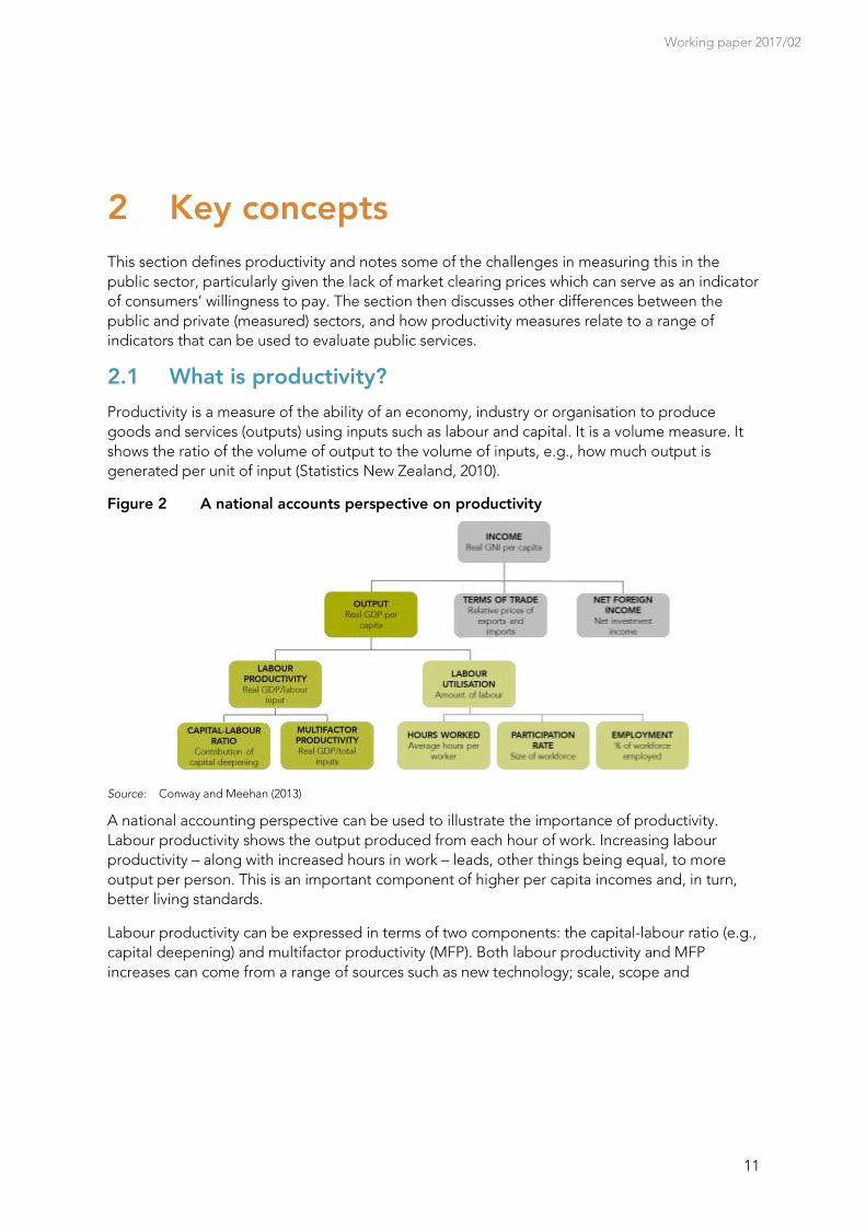
Figure 2 A national accounts perspective on productivity
Source: Conway and Meehan (2013)
A national accounting perspective can be used to illustrate the importance of productivity.
Labour productivity shows the output produced from each hour of work. Increasing labour
productivity – along with increased hours in work – leads, other things being equal, to more
output per person. This is an important component of higher per capita incomes and, in turn,
better living standards.
Labour productivity can be expressed in terms of two components: the capital-labour ratio (e.g.,
capital deepening) and multifactor productivity (MFP). Both labour productivity and MFP
increases can come from a range of sources such as new technology; scale, scope and

Public sector productivity: Quality adjusting sector-level data on New Zealand schools
12
specialisation economies; improvements in firm organisation, management and work practices;
and firm turnover.5
Productivity, technical efficiency and allocative efficiency
Productivity can also be illustrated with a production possibility frontier. This frontier defines the
total output that an economy can produce given its resources. Total output is a function of the
production of a number of goods and services. These goods and services can be produced in
different quantities (reflecting production trade-offs) to give a range of possible total outputs.
When an economy is on the frontier it is impossible to produce more of one good without
producing less of another (all else being equal). However, an economy can move along the
frontier (changing the mix of goods produced) by changing the proportion of inputs used in
production. Further, over time the frontier itself may also shift outwards due to technical
progress. And an economy can become more or less efficient and catch-up to or shift away from
the frontier.
It is important for an economy to be as close to its production possibility frontier as possible,
otherwise some resources are being wasted. When an economy is below its frontier then
opportunities are being missed to increase total output with existing levels of resources. In
other words the economy is said to be lacking technical efficiency. Technical efficiency is a
measure of how far or close an economy is to its production frontier.
Technical efficiency is closely related to the concept of productivity (the ratio with which inputs
can be converted into outputs). Increasing productivity is one way an economy can move closer
to its frontier. Indeed, if inputs are fixed this is the only way. However, even if two economies are
equally productive (e.g., the same distance from the production frontier) they may have different
degrees of allocative efficiency. Allocative efficiency is concerned with the appropriate
distribution of resources to different activities (e.g., doing the right thing, not just doing it in the
right way). It is thus concerned with allocating resources to where they can be economically
most productive (i.e., taking account of relative costs (inputs) and returns (outputs) of different
resource allocations).
2.2 Challenges in applying productivity concepts to public services
While there has been considerable work on productivity in the private sector, much less is
known about the levels, growth rate and determinants of productivity in the public sector. Given
this it can be helpful to define key concepts before seeking to apply them more broadly.
5 There is a distinction between embodied and disembodied change. Only disembodied technological changes are included in multi-factor
productivity (MFP). Some technological changes become embodied in the volume of inputs and so to avoid double counting them they are not
included in MFP. Consider the example of e-mail. This requires some capital deepening (computer servers) and may support and increase in
hours of work (e.g., checking e-mails on a smartphone when out of the office). But it may also improve coordination in the workplace – and it is
this improved coordination that is a disembodied change and included in MFP.
Working paper 2017/02
13
Prices, willingness to pay and the value of outputs
Given the diversity of outputs produced in an economy, productivity measures require an
approach for combining diverse outputs into a single index. Consider the familiar hypothetical
example of an economy that produces only guns and butter. Estimating productivity requires a
measure that combines the output of both these products. But just how many kilos of butter are
equivalent to one gun?
In the private sector prices can be used to make these comparisons. Non-comparable output
volumes can be combined into a single index based on their value in the marketplace. This
approach is followed as prices are generally assumed to be a good indicator of consumers’
valuation of (willingness to pay for) different outputs. It is assumed that if the utility (or benefit)
that a consumer receives from a good or service is less than the market price then the consumer
will not purchase it. A different consumer may have a different willingness to pay and so instead
purchase the good (or purchase different amounts of the good).
Thus in perfect competition different people will consume the product at different levels and
the total level of consumption of the good will reflect the overall utility it provides consumers.
Indeed, an outcome where different people have different preferences and so consume
different amounts of a good could maximise total utility. Perfectly competitive markets allow the
price system to allocate goods among consumers so that each person’s marginal utility from
consumption is equalised. This is a condition for Pareto optimality, as otherwise some of one
person’s consumption could be reallocated to another person who values that consumption
more.
In contrast, public services typically lack, or at best poorly reflect, prices as they are provided
free or at subsidised prices at the point of consumption. As a result, it is not possible to say that
prices for public services necessarily reflect consumers’ willingness to pay, and these prices
cannot therefore be used as proxies for the utility (or value) they generate. Further, value
judgements may be made that the importance of the consumption of some goods means it
should not vary among different consumers (or that it should only vary above a certain “core
consumption” level). This can be the case for so called merit goods. An alternative way of
valuing public services is therefore needed.
An illustration
Productivity is a measure of the effectiveness of a decision making unit at converting inputs into
outputs. As an illustrative example, assume a one output and one input economy in which
productivity can be measured as Q/I, where Q is the output volume and I is the input volume. In
this case there is no difference between labour and multifactor productivity.
But what if we are interested in productivity growth? There are several ways of conceptualising
this: growth in a productivity index, in outputs compared with inputs, and in real revenues with
real costs. The approach taken in this paper is an index approach. Thus productivity growth
between periods 1 (t1) and 2 (t2) equals (Qt2/It2)/(Qt1/It1).
The next step is to account for the fact that there are likely to be multiple inputs and outputs.
One approach is to use input price weights, so labour productivity can be written as Q/wL and
Public sector productivity: Quality adjusting sector-level data on New Zealand schools
14
multi-factor productivity as Q/(wL+rK+mM), where w is the wage rate, L the labour input, r the
rate of return to capital, K the capital input, m the price of intermediate inputs, and M the
intermediate inputs. Likewise, where there are two outputs (a and b), Q is equal to paQa + pbQb,
where pa, pb, Qa, and Qb are the prices and quantities of a and b.
In other words, different types of outputs can be combined into a single index by weighting
their volumes by their market prices.6 In using these weights it is necessary to consider whether
price weights should be fixed over time (using constant or current prices) and, if fixed, for how
long or over what periods (e.g., completed business cycles)?
But there are several challenges in taking a similar approach to measuring public sector
productivity where, at best, there are only proxies for market clearing prices. This means two
things:
In the absence of prices some other alternative is required to combine diverse inputs and
outputs into single input and output indices (weightings).
Unless all prices (p, w, r and m) move together, volume and value based measures will give
different productivity trend results. This is one dimension of the problem of the need for
quality adjustments in measures of public sector productivity.
Other challenges
Even if accurate prices are available, other factors may mean public services require a different
approach to measuring productivity from that used for the measured sector. In particular, the
process of converting inputs into outputs (the productivity of public sector production) is
conditioned by the institutional setting (e.g., regulations, governance structures, etc.). An
observed change in productivity may reflect a change in public policy rather than choices made
by managers in response to consumer demand.7 These institutional arrangements also shape
the degree of innovation in public sector processes (i.e., they have a dynamic effect). A number
of important institutional differences are discussed below. They include differences in the nature
of labour inputs (although these can be overstated), observability of outputs and outcomes,
accountability requirements, and the roles played by competition and consumer choice.
Nature of labour inputs
Public services tend to be relatively labour intensive. This means they can face the so-called
“Baumol cost disease” (Baumol and Bowen, 1966), where wage growth in labour-intensive
industries becomes decoupled from productivity growth. This can happen when productivity
improvements in a capital-intensive industry leads to wage growth in that industry. Competition
6 In the measured sector prices can be used in this way as it is assumed that prices are a good indicator for consumers’ willingness to pay for
different outputs. In a competitive market, the level of consumption of the good will reflect the overall utility it provides consumers. In other
words, “outputs can be measured from market transactions where the dollar volume of products reflects how end users value them” (Hanushek
and Ettema (2015)).
7 An example could include a policy to reduce class sizes. In principle these effects can also occur in the market sector where, for example,
monopoly power held by some suppliers can lead to outputs and prices that reflect producers’ ‘policy’ choices rather than consumers’ marginal
valuation under competitive conditions.
Working paper 2017/02
15
for labour between this industry and other more labour-intensive industries can then mean that
wages in these other industries also grow. This increases the cost of labour inputs relative to the
outputs produced and leads to lower labour productivity. This phenomena can be seen most
clearly in the case of some service industries (Productivity Commission, 2016, p. 63).
As well as differences in labour intensity, public and private (measured) sector employment may
differ in the form of pecuniary incentives offered. The Productivity Commission (2015, appendix
F) distinguished two forms of pecuniary incentives that can operate between a principal and an
agent. High-powered incentives are where an agent receives a large share of some risky
outcome that is affected by their efforts. With low powered incentives the agent’s share of the
risky outcome is small. Public sector workers typically have no claim on residual profits or cost
savings and so their pecuniary incentives tend to be low powered. Public sector workers are also
more likely to have standardised and rigid pay scales – with constraints on pay levels and
performance related pay – and greater job security.
It has also been argued that public sector workers may face greater non-pecuniary incentives,
such as concern about their reputation, mission orientation, etc. According to this view public
sector workers are relatively motivated by non-pecuniary rewards, particularly a shared sense of
mission orientation. Yet, as Le Grand (2007, p. 19) noted, “a review of the available literature on
the motivation of those who work in the public sector suggests, not that they are exclusively
[altruistic] knights or [self-interested] knaves, but, as with most people, a mixture of the two” (Le
Grand, 2007, p. 19). And relying on such an ethos may not be enough as ‘knightly’ people may
not “always be motivated to be very efficient” (e.g., recognise the opportunity cost of the
resources they consume) and have their own agenda (e.g., “give users what the knights think
users need, but not necessarily what the users think they need”) (Le Grand, 2007, pp. 20-21).
Further, it would be incorrect to assume that only workers in public services have a concern for
the welfare of their customers. Indeed, many essential goods and services are provided outside
of the public sector (e.g., food production). And even in cases where essential goods and
services are provided in the public sector (e.g., education and health), these services can often
also be provided by private providers. Thus it is easy to overstate the uniqueness of the labour
input into public services. This means that for productivity measurement many of the techniques
that are used to account for labour input in the private sector (e.g., weighting different
categories of worker by wage rates when combining them into a single index) can be
appropriate for public services.
Observability of outputs and outcomes
An area where there is likely to be a clearer difference between private firms and some
(although not all) public services is the ability to set well defined and measurable goals.
Compared to private sector firms, which may have goals like increased market share or
shareholder value, some public service tasks have relatively complex goals, encompassing, for
example, distributional impacts as well as efficiency. And even where goals can be identified at
Public sector productivity: Quality adjusting sector-level data on New Zealand schools
16
a high level (e.g., investment in human capital), difficulty in observing outputs or outcomes8 and
the role of co-production (e.g., degree to which delivery is self-contained) can mean it is difficult
to define measurable indicators of performance.9 This has implications for the role and form of
productivity analysis (Tavich, 2017).
Lonti and Gregory (2007) and Gregory and Lonti (2008) examined the use of performance
indicators in selected public sector departments in New Zealand and concluded that “despite
the drive to improve managerial performance since the 1990s, indicators tended to address
narrow managerial issues rather than ‘genuinely meaningful measures’” (p.837). More recently
Francis and Horn (2013) argued that New Zealand public service organisations are good at
managing immediate issues and transactional functions, but struggle with building strong
institutions and the strategic and forward looking parts of the system. This highlights the
importance of craft tasks like setting out strategy, leadership and building capability.10 It also
underscores the difficulty of obtaining measures of public sector performance and highlights
the risks of focussing on what can be counted, rather than genuinely addressing the effective
delivery of public services more comprehensively.
Accountability
A further difference reflects the importance of accountability for inputs in public services. A
principle of the state sector reforms in New Zealand in the 1980s was to increase the flexibility
with which managers of public services could manage inputs. The principle was that the political
executive would specify desired outcomes, contract agency chief executives for outputs to
contribute to these outcomes, and agencies would then manage inputs to achieve these
outcomes (letting “managers manage”). Nonetheless, the allocation of inputs (e.g., workers) in
the public sector rightly remains subject to a number of public law and administrative
requirements designed to ensure that public funds are used in a lawful, transparent and
accountable manner.
8 Different public sector tasks present a variety of challenges. As James Wilson (in Gregory, 1995, p. 172) argued, these tasks can be
differentiated according to the observability of their outputs and their outcomes. Consequently four types of task (and examples) can be
identified (Gregory, 1995, p. 173). 1. Production tasks: have both observable outputs and observable outcomes. The purpose is to produce
things. 2. Craft tasks: produce observable outcomes through unobservable work. Often “the successful achievement of desired outcomes is
dependent on the activities of highly trained professionals exercising a large degree of autonomy from day-to-day managerial supervision”
(Gregory, 1995, p. 173). 3. Procedural tasks: are characterised by observable work but unobservable outcomes. The purpose is to maintain
systems. 4. Coping tasks: neither work nor outcomes are observable. Thus not only does work “often require considerable discretion but it also
has ambiguous impacts on the behaviour of ‘clients’ …. They embody objectives that governments do not really know how to achieve”
(Gregory, 1995, p. 173).
9 As Alford (1993, in Gregory, 1995, p. 175) wrote: “Accomplishing the objectives of a government programme can often call for some of the
work to be done by people or organisations other than the producing unit, such as the target group being regulated, or the programmes’
clients, or other public sector agencies, or citizens generally.” (Gregory, 1995, p. 175). This co-production can involve “getting people to act
together even though they do not actually need to agree on why they wish to do so, and can be expected to place differing values on their joint
actions” (Gregory (1995), p. 177). Craft and coping tasks are more likely to rely on co-production than production and procedural tasks.
10 James Q Wilson also discussed the tendency for assignments to be distributed in ways that minimise the chance for key employees to become
expert in their tasks, particularly due to the frequent rotation of assignments. He noted the trade-off between having broadly experienced
employees and having highly expert ones, and that the bias towards frequent rotation reflects incentives to distribute career-enhancing postings
widely rather than just to people most suited for the roles (Wilson, 1989, pp. 171-173).
Working paper 2017/02
17
Yet this emphasis on accountability in public services can come at the expense of a focus on
productivity. As the Productivity Commission (2015) noted agencies may manage performance
risk through highly specified contracts that describe the inputs to be used, the processes to be
followed and the outputs to be produced. This can reduce the incentives and opportunity for
innovation, limit the flexibility of providers to respond to changing needs of clients or changes
in the environment in which services are provided, and limit the scope for providers to work
together and to bundle services in a way that best meets the needs of clients (e.g., service
integration).
In principle, however, concerns with accountability and with productivity are not necessarily
inconsistent. Consider both the government’s purchase and ownership interests in the activities
of departments and Crown entities.11 As Treasury (2011, p. 16) noted:
As a purchaser of outputs (goods and services), “the Government is likely to require
information along the lines of a private sector sales/services contract: provider, quantity,
quality, time and place of delivery and cost.”
As owner, “the Government wants to ensure that capital assets are used efficiently and that
agencies maintain the capability to provide services efficiently and effectively in future years,
in accordance with the Government’s objectives.”
Finally, both “as owner and purchaser, Ministers want to procure quality goods and services
at the right cost, now and into the future.”
Competition and consumer choice (as sources of innovation)
Finally, the mechanism of competition (either in output markets or for the ownership of the firm
itself) is often absent in the public sector. Many public services are delivered by agencies that
face little competition. And while public agencies can be restructured, merged or
disestablished, this tends to be harder to achieve than in the private sector. In contrast, in the
private sector this competition can help drive the reallocation of resources between firms, which
can, in turn, enhance productivity (Conway, 2016).
Public services are also often characterised by the limited role played by consumer choice.
Greater consumer choice can have pros and cons. This choice can drive up quality and efficiency
and ensure that the activities and improvements undertaken ultimately reflect the wishes and
values of the society (better reflect specific client preferences). In cases where greater choice
leads to greater diversity of supply then the provision of services could naturally be less uniform
(Productivity Commission, 2015, p. 44), which may or may not be desirable. And some public
services may be based on paternalistic value judgements (individual users are not believed to
11 For example, in relation to the purchasing interest a key principle is that the Crown cannot spend public money except by or under an Act of
Parliament. In most cases this authority is achieved through Appropriation Acts presented as part of the Government’s budget package
(Treasury, 2011, p. 13). Appropriations are limited to a maximum level of spending, to a particular period, and to uses set by the scope
statement. Appropriations group outputs purchased by Ministers into output classes that contain different outputs contributing to a common
outcome. These outputs are the basis of purchase agreements between Ministers and government agencies (Treasury, 2011, p. 14).

Public sector productivity: Quality adjusting sector-level data on New Zealand schools
18
be the best judges of their needs) and so the case for responding to client preferences is
attenuated.
Nevertheless, the absence of competition and choice can be overstated, as in practice many
public services are usually provided as mixed model systems (e.g., with private as well as public
providers). Mixed model systems can generate a number of benefits. From a national-economy
perspective a private pillar can, for example, make the welfare state more efficient by increasing
the range of tools available for smoothing consumption and spreading risk. By reducing fiscal
pressure on the public system this can mean programmes are more affordable for governments
in the long run (although this may be undermined by policies like poorly designed funding
systems). A mixed model also has important political effects, with a stronger private pillar
helping to build consensus that funding the welfare state requires a team effort (Nolan et al.,
2012).
Indeed, expanding the roles of competition and choice was seen as a key mechanism for
improving the performance of public services in the United Kingdom during the later years of
the Blair government. As Le Grand (2006) noted it was argued that the:
reforms involving choice and competition that the Government of Tony Blair [introduced] into public services such as health and education will make those services not only more responsive and more efficient, but also ... more equitable or socially just.
The benefits from government efforts to extend competition and choice were expected to
particularly benefit the less well off, as middle income groups were seen as the major
beneficiary of “unreformed no-choice” systems. As Le Grand (2006) wrote: “With their loud
voices, sharp elbows and, crucially, their ability to move house if necessary, the middle class get
[…] more hospital care relative to need, more preventive care, and better schools.”
2.3 Productivity and public sector performance metrics
What does the above discussion mean for the role of productivity in performance measurement
in government services? In the first place it highlights that productivity is only one possible
indicator of the performance of the public sector. This can be illustrated in the model
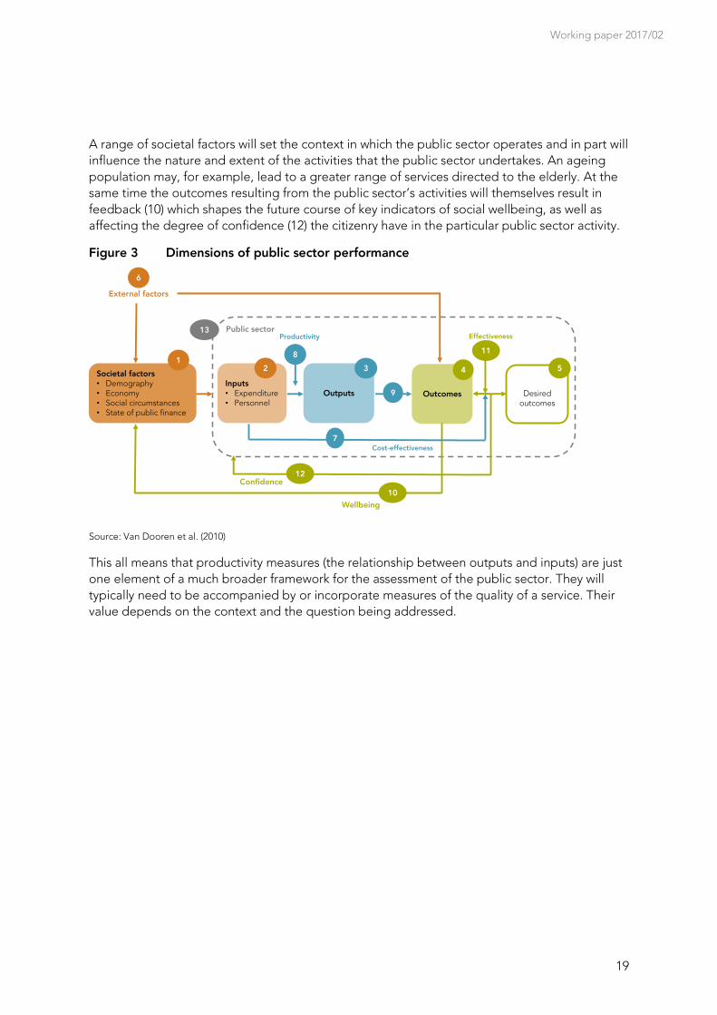
developed by van Dooren et al. (2010), shown in Figure 3.
Productivity (8) lies at the core of the framework and relates the output of goods and services (3)
generated by the public sector (13) to the inputs used in the production of those goods and
services (2). The next step in the framework highlights the fact that that productivity is not
necessarily an end in itself. In fact it is possible for productivity to be improved with no
consequent change in outputs (3) or intermediate outcomes (4). In many cases a more
comprehensive view of productivity will be required: one that traces the links (9) from outputs to
outcomes.
However, for many reasons intermediate outcomes (4) may not necessarily coincide with the
desired (final) outcomes (5). For example, external factors (6) may influence the actual outcomes
such that they deviate from the desired outcomes, so reducing the effectiveness (11) of the
particular policy or activity. It is the relation between the actual outcomes (4) and the inputs (7)
that determines the value for money (or cost effectiveness) of the public activity.
Working paper 2017/02
19
A range of societal factors will set the context in which the public sector operates and in part will
influence the nature and extent of the activities that the public sector undertakes. An ageing
population may, for example, lead to a greater range of services directed to the elderly. At the
same time the outcomes resulting from the public sector’s activities will themselves result in
feedback (10) which shapes the future course of key indicators of social wellbeing, as well as
affecting the degree of confidence (12) the citizenry have in the particular public sector activity.
Figure 3 Dimensions of public sector performance
Source: Van Dooren et al. (2010)
This all means that productivity measures (the relationship between outputs and inputs) are just
one element of a much broader framework for the assessment of the public sector. They will
typically need to be accompanied by or incorporate measures of the quality of a service. Their
value depends on the context and the question being addressed.
External factors
Outputs Outcomes Desiredoutcomes
Effectiveness
Inputs• Expenditure• Personnel
Confidence
Societal factors• Demography• Economy• Social circumstances• State of public finance
Wellbeing
Cost-effectiveness
Public sectorProductivity
6
1
13
2 3 4
11
5
7
12
10
8
9
Public sector productivity: Quality adjusting sector-level data on New Zealand schools
20
3 The existing picture
A number of OECD countries are giving increased attention to measuring elements of the non-
measured sector (particularly the public sector) or, in some cases, estimates of aggregate public
sector productivity. At the forefront of these developments has been the Office for National
Statistics (ONS) in the United Kingdom. Progress has also been made by Statistics New Zealand.
For many years the default position in measuring the output of the public sector was to largely
assume the growth rate of output was equal to the growth of inputs. This is the inputs equals
outputs convention. This approach reflected the absence of prices and directly observed output
measures for publicly provided goods and services but effectively assumed away the question of
productivity. It implied that the social value of the government outputs was always proportional
to the cost of the inputs. There was limited value in such an approach.
Since the early part of this century serious efforts have been made to move beyond the inputs
equals outputs convention. In the United Kingdom impetus came as the result of an
independent review of the measurement of government output and productivity commissioned
in 2003 by the ONS and led by Sir Tony Atkinson. This followed a European Commission
requirement that direct measures of output should be incorporated in the national accounts by
2006. The Atkinson report (2005a and 2005b) was positively received by the then National
Statistician, Len Cook, and led to the establishment of a Centre for the Measurement of
Government Activity (UKCeMGA) within the ONS. UKCeMGA operated between 2005 and 2010
and carried out an extensive programme of development work, including establishing a
methodology for estimating productivity growth in key public services.
3.1 The Statistics New Zealand approach
In New Zealand, Statistics New Zealand regularly publishes estimates for education and training
and healthcare and social assistance as part of their annual releases of industry-level productivity
measures. Details of the methodology are given in Statistics New Zealand (2013) and Tipper
(2013). As Tipper (2013) noted education and healthcare were prioritised as these are areas
where most progress has been made in defining output measures. Defining output in collective
services, such as defence, police or fire services, remains relatively difficult.
Output measures are based on a chain-volume value added, GDP production approach. Value
add is defined as output minus intermediate consumption. This approach is designed to
overcome the absence of market prices in these sectors. Once activity measures have been
defined their growth rates are computed. To the extent there are activities in the subsectors
which are not measured, it is assumed that their growth rates are the same as those of the
measured activities.
The growth rates of the activities are then combined into a single output index for the subsector
using cost weights for the different components of output which reflect their relative
importance. Tipper (2013) notes that in the absence of market-clearing prices the international
consensus is that it is appropriate to use cost weights, which reflect the value placed on the

Working paper 2017/02
21
service by the producer (Dawson et al., 2005). Cost weights are also available for most types of
education and healthcare and can be updated annually (Tipper, 2013, p. 9).
In the case of inputs, measures of labour and capital used in the production of the activities are
estimated and combined. The labour input is based on hours paid, while the capital input is
estimated by applying the user cost of capital to the total capital stock used in the industry. The
latter is constructed using the perpetual inventory method (PIM). An exogenously given rate of
return of 4% is applied to all industries in the estimation of the user cost of capital (Macgibbon,
2010).
More specifically, in the case of education and training, overall output is constructed by
combining preschool education (contributing 8% of value add to the sector), school education
(contributing 50%), tertiary education (contributing 33%), adult, community and other education
(contributing 8%) (Tipper, 2013, p. 13). The output indicator for each sub-sector is based on
cost-weighted number of equivalent full-time students (EFTS). Cost weights are derived from
financial data on expenditures for each activity. There is a proportion of the activities that is not
measured (including research). Their growth rates are therefore assumed to match those of the
measured activities.12
3.2 Aggregate labour productivity
The data sources described above can be used to derive measures of labour productivity in the
public sector. These can then form the basis of comparisons with labour productivity in the
measured sector, as well as comparisons between New Zealand and Australia.
Data from Statistics New Zealand on the relative performance of the measured and public
sectors in New Zealand between 1996 and 2014 are summarised in Table 2. Estimates for these
sectors are combined to provide a measure of productivity for the total economy. The public
sector data are not explicitly adjusted for quality. Nonetheless, these data show:
For the total economy, New Zealand’s lower output growth reflected both a slower rate of
growth of labour input and lower overall growth in productivity than in Australia.
For the measured sector, productivity growth was markedly lower in New Zealand than in
Australia. This was a major contributor to the stronger output growth in this sector in
Australia.
For the public sector, in both New Zealand and Australia productivity growth was only 13%
of the average growth rate in the measured sector, implying that despite New Zealand’s low
12 For completeness, the Statistics New Zealand approach to constructing health sector output is discussed below (Tipper, 2013, p. 21). Overall
output combines hospitals (contributing 45% of value add to the sector), medical and other healthcare services (contributing 34%), and
residential care services and social assistance (contributing 21%). The market component of these services is 43% (made up of 2% in hospitals,
30% in medical services and 11% in residential services). The output indicator for hospitals is based on inpatient and day patient events
(weighted by the nature of the diagnosis and the length of stay) and emergency department and outpatient services. These are combined using
cost weights. Medical and other healthcare services include general practitioners and dentists. There is a proportion of the activities that are not
measured (including mental health services). Their growth rates of output are assumed to simply match those of the measured activities.
Public sector productivity: Quality adjusting sector-level data on New Zealand schools
22
rate of productivity growth in the public sector, the gap relative to the measured sector is
broadly consistent with that in Australia.
Table 2 Average annual rates of growth in labour productivity: New Zealand and Australia (1996-2014)
Measured sector Public sector Total economy
New Zealand Australia New Zealand Australia New Zealand Australia
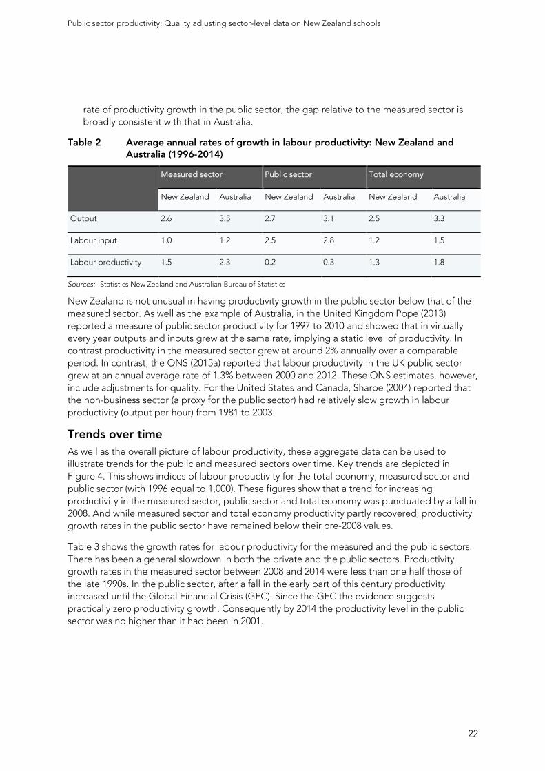
Output 2.6 3.5 2.7 3.1 2.5 3.3
Labour input 1.0 1.2 2.5 2.8 1.2 1.5
Labour productivity 1.5 2.3 0.2 0.3 1.3 1.8
Sources: Statistics New Zealand and Australian Bureau of Statistics
New Zealand is not unusual in having productivity growth in the public sector below that of the
measured sector. As well as the example of Australia, in the United Kingdom Pope (2013)
reported a measure of public sector productivity for 1997 to 2010 and showed that in virtually
every year outputs and inputs grew at the same rate, implying a static level of productivity. In
contrast productivity in the measured sector grew at around 2% annually over a comparable
period. In contrast, the ONS (2015a) reported that labour productivity in the UK public sector
grew at an annual average rate of 1.3% between 2000 and 2012. These ONS estimates, however,
include adjustments for quality. For the United States and Canada, Sharpe (2004) reported that
the non-business sector (a proxy for the public sector) had relatively slow growth in labour
productivity (output per hour) from 1981 to 2003.
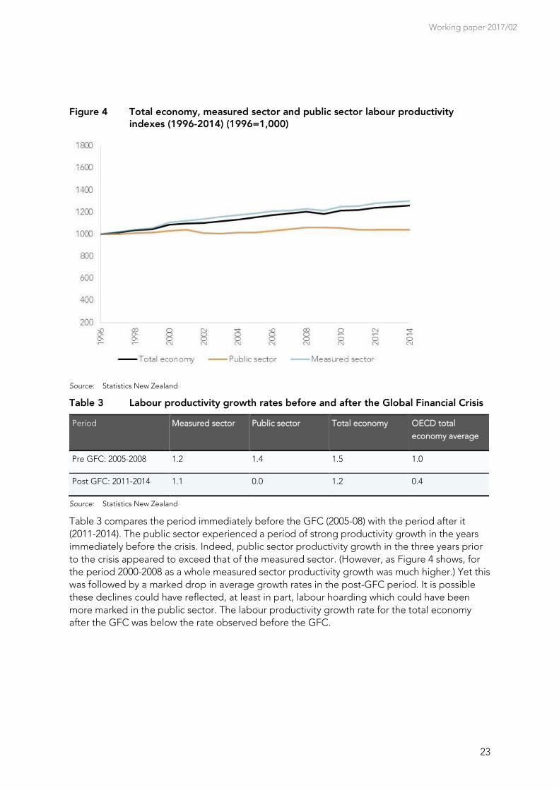
Trends over time
As well as the overall picture of labour productivity, these aggregate data can be used to
illustrate trends for the public and measured sectors over time. Key trends are depicted in
Figure 4. This shows indices of labour productivity for the total economy, measured sector and
public sector (with 1996 equal to 1,000). These figures show that a trend for increasing
productivity in the measured sector, public sector and total economy was punctuated by a fall in
2008. And while measured sector and total economy productivity partly recovered, productivity
growth rates in the public sector have remained below their pre-2008 values.
Table 3 shows the growth rates for labour productivity for the measured and the public sectors.
There has been a general slowdown in both the private and the public sectors. Productivity
growth rates in the measured sector between 2008 and 2014 were less than one half those of
the late 1990s. In the public sector, after a fall in the early part of this century productivity
increased until the Global Financial Crisis (GFC). Since the GFC the evidence suggests
practically zero productivity growth. Consequently by 2014 the productivity level in the public
sector was no higher than it had been in 2001.
Working paper 2017/02
23
Figure 4 Total economy, measured sector and public sector labour productivity indexes (1996-2014) (1996=1,000)
Source: Statistics New Zealand
Table 3 Labour productivity growth rates before and after the Global Financial Crisis
Period Measured sector Public sector Total economy OECD total
economy average
Pre GFC: 2005-2008 1.2 1.4 1.5 1.0
Post GFC: 2011-2014 1.1 0.0 1.2 0.4
Source: Statistics New Zealand
Table 3 compares the period immediately before the GFC (2005-08) with the period after it
(2011-2014). The public sector experienced a period of strong productivity growth in the years
immediately before the crisis. Indeed, public sector productivity growth in the three years prior
to the crisis appeared to exceed that of the measured sector. (However, as Figure 4 shows, for
the period 2000-2008 as a whole measured sector productivity growth was much higher.) Yet this
was followed by a marked drop in average growth rates in the post-GFC period. It is possible
these declines could have reflected, at least in part, labour hoarding which could have been
more marked in the public sector. The labour productivity growth rate for the total economy
after the GFC was below the rate observed before the GFC.
Public sector productivity: Quality adjusting sector-level data on New Zealand schools
24
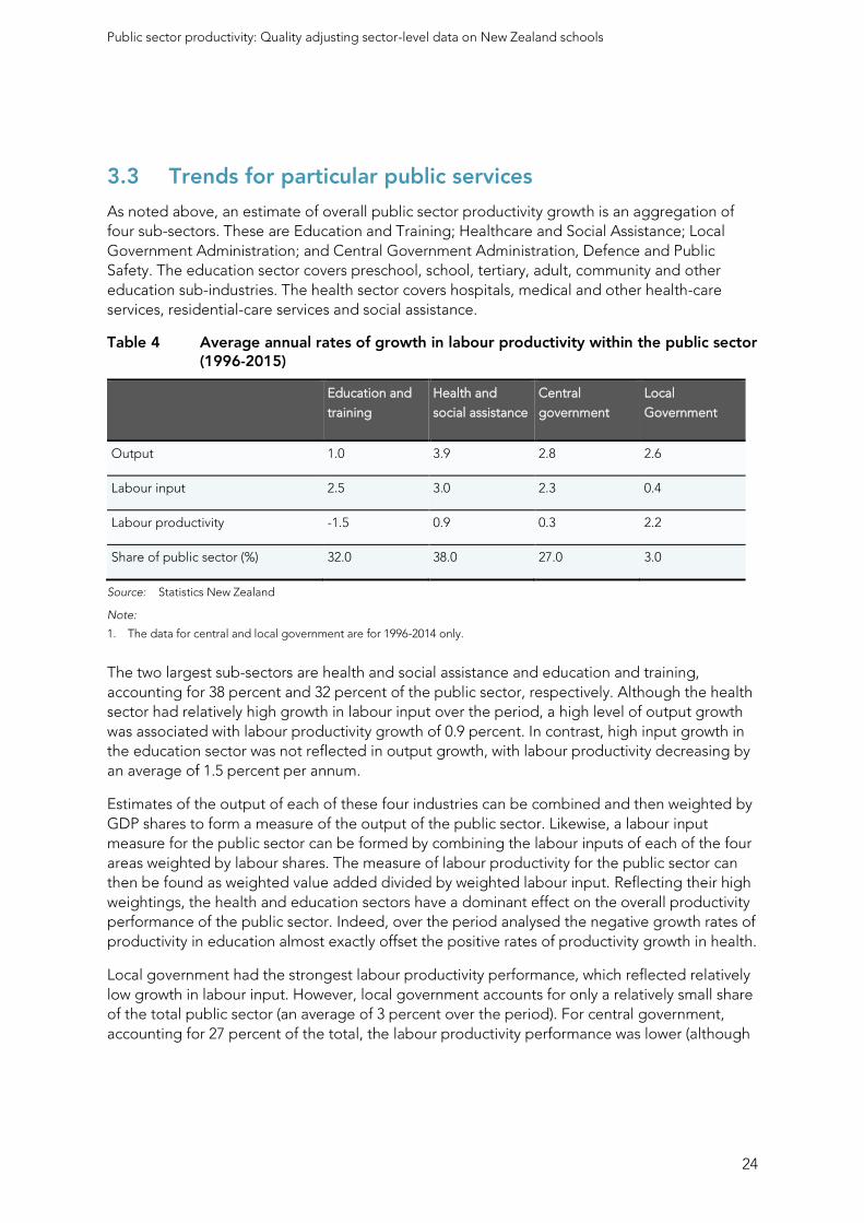
3.3 Trends for particular public services
As noted above, an estimate of overall public sector productivity growth is an aggregation of
four sub-sectors. These are Education and Training; Healthcare and Social Assistance; Local
Government Administration; and Central Government Administration, Defence and Public
Safety. The education sector covers preschool, school, tertiary, adult, community and other
education sub-industries. The health sector covers hospitals, medical and other health-care
services, residential-care services and social assistance.
Table 4 Average annual rates of growth in labour productivity within the public sector (1996-2015)
Education and
training
Health and
social assistance
Central
government
Local
Government
Output 1.0 3.9 2.8 2.6
Labour input 2.5 3.0 2.3 0.4
Labour productivity -1.5 0.9 0.3 2.2
Share of public sector (%) 32.0 38.0 27.0 3.0
Source: Statistics New Zealand
Note:
1. The data for central and local government are for 1996-2014 only.
The two largest sub-sectors are health and social assistance and education and training,
accounting for 38 percent and 32 percent of the public sector, respectively. Although the health
sector had relatively high growth in labour input over the period, a high level of output growth
was associated with labour productivity growth of 0.9 percent. In contrast, high input growth in
the education sector was not reflected in output growth, with labour productivity decreasing by
an average of 1.5 percent per annum.
Estimates of the output of each of these four industries can be combined and then weighted by
GDP shares to form a measure of the output of the public sector. Likewise, a labour input
measure for the public sector can be formed by combining the labour inputs of each of the four
areas weighted by labour shares. The measure of labour productivity for the public sector can
then be found as weighted value added divided by weighted labour input. Reflecting their high
weightings, the health and education sectors have a dominant effect on the overall productivity
performance of the public sector. Indeed, over the period analysed the negative growth rates of
productivity in education almost exactly offset the positive rates of productivity growth in health.
Local government had the strongest labour productivity performance, which reflected relatively
low growth in labour input. However, local government accounts for only a relatively small share
of the total public sector (an average of 3 percent over the period). For central government,
accounting for 27 percent of the total, the labour productivity performance was lower (although
Working paper 2017/02
25
still positive), which reflected a similar level of output growth but higher level of labour input
growth.
3.4 What other studies tell us
There is a sizeable literature containing detailed comparisons of performance of the education
sector.13 Dutu and Sicari (2016) provide a recent contribution. They argue (p. 7) that an
“approach based on spending areas rather than overall public sector efficiency is generally
considered more effective when dealing with cross-country data.” This is because sectors may
have a variety of objectives and differ in the ways in which output can be specified. Further, a
focus on a single sector makes it easier to identify performance, as a country’s overall
performance may mask differences across sectors.
A large number of studies have suggested that the New Zealand education system performs
relatively well. For example, Afonso and Aubyn (2005) found that in 2000 New Zealand schools
ranked 5th of 17 countries for output efficiency and 8th of 17 for input efficiency. Sutherland et al.
(2007) found that New Zealand ranked 6th out of 30 countries for input efficiency. Schreyer (2010)
reported that for experimental calculations of educational outputs in 2005 New Zealand was
ranked 4th of 33 countries.
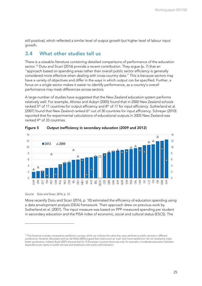
Figure 5 Output inefficiency in secondary education (2009 and 2012)
Source: Dutu and Sicari, 2016, p. 12
More recently Dutu and Sicari (2016, p. 10) estimated the efficiency of education spending using
a data envelopment analysis (DEA) framework. Their approach drew on previous work by
Sutherland et al. (2007). The input measure was based on PPP-measured spending per student
in secondary education and the PISA index of economic, social and cultural status (ESCS). The
13 This literature includes comparative satisfaction surveys, which can indicate the value that users attribute to public services in different
jurisdictions. However, Bouckaert and van de Walle (2003) argued that criteria such as ‘trust’ and ‘more satisfaction’ do not necessarily imply
better governance. Indeed, Boyle (2007) showed that for 15 European countries there was only, for example, a moderate association between
expenditure per capita on public services and satisfaction with public administration.
Public sector productivity: Quality adjusting sector-level data on New Zealand schools
26
output variable was a synthetic PISA score based on the average country scores for reading,
mathematics and science.
These data showed that between 2006-08 and 2009-11 this measure of education sector
performance in New Zealand moved closer to (although remaining better than) the OECD
average. Output inefficiency had significantly worsened in New Zealand, and the sector’s
ranking had slipped from 2nd to only just above the OECD average (13th of 30). Likewise, input
inefficiency had also significantly worsened with New Zealand falling to just above the OECD
average (12th of 30). This deterioration in the ranking can be explained by a weakening of PISA
scores coupled with increased spending. By these measures New Zealand had thus fallen from
having one of the best performing school systems to having an average performing one.
Data Envelopment Analysis (DEA) techniques (see Appendix C) have also been used to assess
the performance of different schools within New Zealand. Factors studied have included
ownership type, single-sex/co-educational, location and scale. Alexander and Jaforullah (2005)
and Alexander et al. (2007), for example, found scale disadvantages were evident in rural
schools, integrated schools generally outperformed state schools and single-sex schools
outperformed co-educational ones. Harrison and Rouse (2014) found that higher performance
was associated with higher competition (moderated by school size) and that a widening gap in
performance was observed between the largest and smallest schools.14
3.5 Quality adjustments
The presence or otherwise of quality adjustments can play an important role in the
interpretation of productivity data (Maimaiti and O’Mahony, 2011). However, while important,
adjusting estimates of public sector productivity for quality can be complex. Further, as Schreyer
and Lequiller (2007) noted, information beyond that contained in the national accounts will
generally be needed in order to adjust for quality. And as quality is multi-dimensional a single
index is unlikely to be adequate.
Some of the challenges in making quality adjustments in the education sector are discussed in
detail below and can be illustrated with the case of the United Kingdom. In this country the ONS
has had to revise its approach to adjusting education outputs for quality, given an increase in
the numbers of students sitting non-GCSE exams (the main United Kingdom exams at age 16).
This is not a trivial matter, as any adjustment makes a substantial difference to measured
productivity. From 1997 to 2011, measured output growth in the education sector of the United
Kingdom grew at an annual average rate of 2.7%. Of this the quality adjustment accounted for
90%, or an annual rate of growth of 2.5% (Caul, 2014, p. 8).
14 Data Envelopment Analysis (DEA) techniques have also been used to investigate the performance of the New Zealand tertiary education
sector. For instance, Smart (2009) and Margaritis and Smart (2011) found that the productivity growth of New Zealand universities between 1997
and 2005 was lower than that of the G8 and newer universities in Australia. They also noted that the introduction of the Performance Based
Research Fund (PBRF) stimulated productivity improvements in the New Zealand university sector, as a result of increased research output.
Abbott and Doucouliagos (2009) showed that in New Zealand enrolments of overseas students appeared to have had no effect on technical
efficiency, which contrasted with the picture from Australian universities. Talukder (2011) found that private providers experienced a larger MFP-
growth than that of public providers during 1999-2004, but also experienced a sharper decline in MFP-growth since 2000 through to 2010.

Working paper 2017/02
27
In New Zealand, Tipper (2013) argued that the decision not to make explicit adjustments for
quality in the education and health measures reflects the absence of an internationally agreed
set of standards and limitations of the data. There is, however, an implicit quality adjustment
made. As the measures have been complied at a disaggregated level this allows for changes in
the composition of output. Yet this method only captures that part of the total potential
changes in quality that are associated with compositional shifts (Sharpe et al., 2007). It fails to
capture quality changes at the level of the individual intervention. And when costs are used as
weights for groups of activities there is also a presumption that higher costs equate to higher
quality. For these reasons Atkinson (2005a) favoured weighting by a measure of the quality of
actual outcomes rather than by costs.
The Office for National Statistics approach
The Office for National Statistics (ONS) estimates of public sector productivity growth are built
up from estimates of growth rates in nine subsectors. For six of these areas separate estimates
of output, inputs and productivity are produced. These are healthcare, education, adult social
care, children’s social care, public order and safety, and social security administration. A further
three areas are treated as collective services and so the inputs equals outputs convention is
adopted. These are police, defence, and other services (including general government services,
economic affairs, environmental protection, housing and recreation). Productivity is by definition
constant for these other services.
Productivity growth for total public services is estimated by combining growth rates for
individual subsectors using their relative share of total government expenditure (expenditure
weights). For most service areas output is measured by activities performed and services
delivered. Quality adjustments are made to outputs in health and education. Inputs are made
up of volume measures of labour, goods and services, and capital, and are mostly measured
using current expenditure adjusted by a suitable deflator. Particular features of the approaches
taken in education are summarised below.15
The quantity of education services is the sum, weighted by cost, of full-time equivalent and
publicly funded pupil and student numbers for pre-school education, government maintained
primary, secondary and special schools, and further education colleges. Student and pupil
numbers are adjusted for attendance (Caul, 2014). As the focus is on measuring productivity in
publicly-funded education, independent schools and higher education (other than training
teachers and some health professionals) are excluded from these estimates (Bridge, 2015).
Quantity is adjusted for the Level 2 attainment by students in England, a five year geometric
average of average point scores for students at this level in Scotland, and average point scores
15 For completeness the ONS approach to quality adjusting healthcare is briefly discussed below. The quantity of healthcare services is
constructed by combining hospital and community health services, family health services, GP prescribing and non-NHS output into an activity
index with weights given by unit costs. For non-NHS services, which account for approximately 9% of healthcare output, the inputs equals
outputs rule is applied. A quality adjustment is then applied to the quantity of healthcare to give healthcare output. The quality adjustment is
based on health gain, short-term survival rates, waiting times, results from the National Patient Survey and selected primary care measures
(Office for National Statistics, 2013a). Labour inputs are based on full-time equivalent employee numbers. Goods and services and capital
consumption are based on current price expenditure divided by appropriate deflators.

Public sector productivity: Quality adjusting sector-level data on New Zealand schools
28
for GCSEs in Wales. Output for all countries had previously been based on changes in average
point scores at GCSE or equivalent level, but this was no longer appropriate in the face of
increases in the number of non-GCSE examinations. Local government labour inputs are based
on full-time equivalent teacher and support staff numbers adjusted for hours worked. Central
government labour inputs, goods and services and capital consumption are based on current
price expenditure divided by appropriate deflators.
Quality adjustments in education
In education, key quality adjustments can relate to inputs (e.g., teacher quality or pupil-staff
ratios), outputs (e.g., school inspectors or educational attainment) or outcomes (e.g., impact on
human capital or house prices), the latter aiming to capture the impact of school zoning (Howell,
2016). Some of the key challenges in making a quality adjustment for education are shown in
Table 5.
As Howell (2016) noted there are a number of studies on teacher quality. This reflects evidence
that suggests that teacher quality is the single biggest influence on pupils’ educational progress
(e.g., Hanushek and Rivkin, 2006). In the United Kingdom, Kimbugwe, Lewis and James (2009)
suggested that labour inputs should be quality adjusted in order to recognise improvements in
teachers’ quality over time. They argued for accounting for quality by measuring the quantity of
labour using either actual hours worked, hours paid or FTE number of employees broken down
by type of employee.
Class size (pupil-staff ratios) are often cited as an indicator for educational quality. However, the
evidence on this link is mixed. To name a few studies, for example, Rivkin et al. (2005), Bowles,
Gintis and Osborne (2001) and Collesi et al. (2007) have all drawn different conclusions
regarding class size and teaching quality. Class size should be seen as one of many components
that may make up teaching quality. There is also a question of at what number of students do
any negative effects of congestion start to take effect. Nonetheless, adjustments for class size
are relatively simple in their application and are used in a number of countries (Howell, 2016).
They do, however, need to be interpreted with caution.
School inspection reports could be useful as a form of quality adjustment as their purpose is to
identify and judge characteristics of the education delivered at schools that are valued by the
students, educators and parents (Schreyer, 2010). There are also, however, challenges in using
inspections as a basis for quality adjustment. Inspections are largely qualitative and may be
subject to personal biases of particular inspectors (Schreyer, 2010). The criteria for defining
good or bad performance may also change over time. It is also necessary to find some approach
to weighting individual inspections so they are comparable over time and across schools, such
as through an overall effectiveness score for schools (Department for Education and Skills,
2005).16
16 In the United Kingdom Ofsted has calculated overall effectiveness scores for schools. These incorporate the quality of teaching, pupils’
achievement, leadership and management, and personal development, including attitude and behaviour. The score also considered the context
of the school and how it performs compared to similar schools (Department for Education and Skills, 2005).
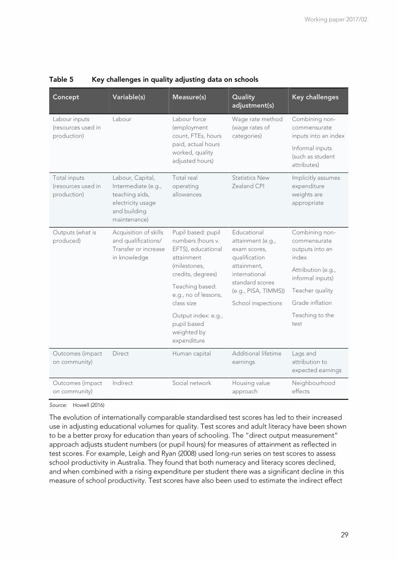
Working paper 2017/02
29
Table 5 Key challenges in quality adjusting data on schools
Concept Variable(s) Measure(s) Quality
adjustment(s)
Key challenges
Labour inputs
(resources used in
production)
Labour Labour force
(employment
count, FTEs, hours
paid, actual hours
worked, quality
adjusted hours)
Wage rate method
(wage rates of
categories)
Combining non-
commensurate
inputs into an index
Informal inputs
(such as student
attributes)
Total inputs
(resources used in
production)
Labour, Capital,
Intermediate (e.g.,
teaching aids,
electricity usage
and building
maintenance)
Total real
operating
allowances
Statistics New
Zealand CPI
Implicitly assumes
expenditure
weights are
appropriate
Outputs (what is
produced)
Acquisition of skills
and qualifications/
Transfer or increase
in knowledge
Pupil based: pupil
numbers (hours v.
EFTS), educational
attainment
(milestones,
credits, degrees)
Teaching based:
e.g., no of lessons,
class size
Output index: e.g.,
pupil based
weighted by
expenditure
Educational
attainment (e.g.,
exam scores,
qualification
attainment,
international
standard scores
(e.g., PISA, TIMMS))
School inspections
Combining non-
commensurate
outputs into an
index
Attribution (e.g.,
informal inputs)
Teacher quality
Grade inflation
Teaching to the
test
Outcomes (impact
on community)
Direct Human capital Additional lifetime
earnings
Lags and
attribution to
expected earnings
Outcomes (impact
on community)
Indirect Social network Housing value
approach
Neighbourhood
effects
Source: Howell (2016)
The evolution of internationally comparable standardised test scores has led to their increased
use in adjusting educational volumes for quality. Test scores and adult literacy have been shown
to be a better proxy for education than years of schooling. The “direct output measurement”
approach adjusts student numbers (or pupil hours) for measures of attainment as reflected in
test scores. For example, Leigh and Ryan (2008) used long-run series on test scores to assess
school productivity in Australia. They found that both numeracy and literacy scores declined,
and when combined with a rising expenditure per student there was a significant decline in this
measure of school productivity. Test scores have also been used to estimate the indirect effect

Public sector productivity: Quality adjusting sector-level data on New Zealand schools
30
of public services on economic growth. Hanushek et al. (2010) used PISA scores to model the
long-run economic impact of attainment levels of students in OECD countries.
Another approach draws on a human capital framework, in which education is viewed as an
investment. The payoff to this investment comes in the form of higher expected future earnings,
which capture at least one dimension of the outcomes of the education process. Examples
include:
Murray (2007): uses both test scores and expected earnings to derive a quality adjusted
measure of the output of Scottish schools.
O’Mahony and Stevens (2009): use the number of fulltime equivalent students enrolled as
their basic output measure to compare productivity growth in the education sectors of the
United States and the United Kingdom. This is augmented with earnings outcomes for each
educational/qualification level conditioned on the probability of employment. Further
adjustment is made to capture quality changes that arise within educational levels due to
innovations in teaching methods or curricula. The authors also adjust earnings based on age
cohorts.
Barslund and O’Mahony (2012): use future prospective earnings as a measure of the value of
additional education. O’Mahony et al. (2012) apply this to measuring output growth in the
post-compulsory education sector in Europe.
Hanushek (2010) focuses on earnings as a way of estimating the value of teacher quality.
There are, of course, limitations to using expected earnings as a measure of the value of
education. The method can be influenced by selection bias, where students enrolling in
additional education are self-selecting (i.e., they do not constitute a random sample). Second,
the historical earnings profiles for different levels of qualification are typically used as the basis
for future earnings but the past is not always a good predictor of the future. Third, any earnings
premium is often attributed to education when some part of this may have been due to a
person’s innate abilities, their family backgrounds, health status or the influence of their peers,
employer provided training, and so on (Hanushek, 2015).
A novel approach to assessing the quality of school education adopted by Black (1998) was to
analyse the difference in prices for equivalent houses in the same neighbourhood in Boston but
belonging to different school zones. In similar work for Christchurch, New Zealand, Gibson and
Boe-Gibson (2014) found that a one standard deviation in higher pass rates in NCEA
examinations was associated with a 6.4% higher house price index in that zone, all else being
equal. However, as Howell (2016) notes, this approach needs to account for any potential
neighbourhood effects which also affect house prices and a school may enjoy a better
reputation or status despite not being of better quality than comparator schools (e.g., when
measured against student test scores).
A final, more general, issue noted by Atkinson (2005a) reflects any interdependence between
the value of public sector outputs and economic growth. Atkinson (2005a) argues that, reflecting
the rise in the real value of private assets and incomes, the output of public services (e.g.,
Working paper 2017/02
31
education, firefighting, postal services, health, etc.) becomes more valuable with the passing of
time. For example, the benefit of saving a house from a fire rises with the value of the house and
its contents. Atkinson (2005a) thus argued that cost weights need to incorporate the effect of
these changes in value.
3.6 Quality adjustments in this paper
The quality of a product or service may vary over time as it is refined and developed or as the
producers’ operating environment changes. These changes can affect productivity trends. Yet
as important as quality adjustments are, there is no international consensus on the appropriate
way to account for them in public services (Statistics New Zealand, 2010; Tipper, 2013).17
Schreyer (2010) outlines three approaches to adjusting for quality changes in education.
Since different types of education call for different approaches to teaching, an analysis of
productivity can be done by stratifying different educational products. This amounts to an
implicit form of quality adjustment and is the approach taken by Statistics New Zealand.
An explicit quality adjustment can be made by, for example, adjusting labour inputs by wage
rates or outputs by examination scores or attainment levels (O’Mahony and Stevens, 2009).
Indirect outcome measures such as future earnings can be used as a proxy for the
underlying quality of the education. As noted above, some studies have used prices of
houses adjacent to schools with different performance ratings as an indicator of school
quality (Black, 1998; Gibson and Boe-Gibson, 2014; Cannon et al., 2015).18
No single measure can capture the full richness of the productivity story. In this paper a number
of explicit quality adjustments have thus been used.
Table 6 summarises the measures used in this paper. To illustrate the potential of existing data
and to also allow these measures to be replicated emphasis was given to using sector-level data
from publicly available sources. The advantage of sector-level data is that it can be potentially
comprehensive, although these data do not address the distribution of outcomes across
decision making units. Sources have included Statistics New Zealand, the Ministry of Education,
and the Treasury. Statistics New Zealand provided some additional data from the New Zealand
Income Survey and Ministry of Education provided data for earlier years for some selected
variables. Where data are available results are shown for 1997 to 2015. In some cases data were
only available to 2014 or (only available in a consistent way) from 2002. The overall summary of
all measures is thus restricted to 2002 to 2014.
17 Accounting for quality adjustment can also be difficult in the measured sector – e.g. where innovation is associated with better quality
products at initially higher, but then potentially falling, prices.
18 Evidence for New Zealand comes from a study of house prices in pre-earthquake Christchurch by Gibson and Boe-Gibson (2014). They find
that house prices in school zones where the schools have higher NCEA pass rates attract a price premium. For example a 7 percentage point
rise in NCEA level 1 pass rates is associated with an increase in mean house prices of $16,000 (in 2005 dollars). This effect is after controlling for
12 characteristics of the house, and 21 characteristics of the mesh block in which the house is located. Other studies for New Zealand that
estimate the effect of zoning but not school quality explicitly include McClay and Harrison (2003), Gibson et al. (2007) and Rehm and Filippova
(2008).
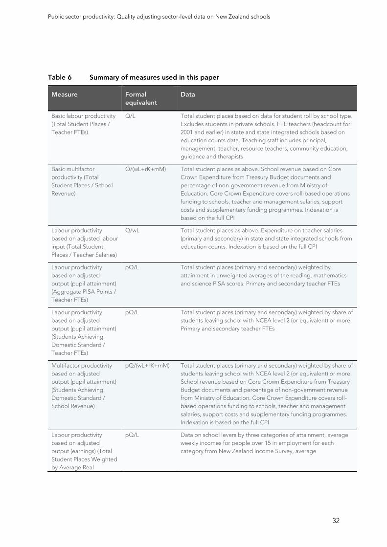
Public sector productivity: Quality adjusting sector-level data on New Zealand schools
32
Table 6 Summary of measures used in this paper
Measure Formal
equivalent
Data
Basic labour productivity
(Total Student Places /
Teacher FTEs)
Q/L Total student places based on data for student roll by school type.
Excludes students in private schools. FTE teachers (headcount for
2001 and earlier) in state and state integrated schools based on
education counts data. Teaching staff includes principal,
management, teacher, resource teachers, community education,
guidance and therapists
Basic multifactor
productivity (Total
Student Places / School
Revenue)
Q/(wL+rK+mM) Total student places as above. School revenue based on Core
Crown Expenditure from Treasury Budget documents and
percentage of non-government revenue from Ministry of
Education. Core Crown Expenditure covers roll-based operations
funding to schools, teacher and management salaries, support
costs and supplementary funding programmes. Indexation is
based on the full CPI
Labour productivity
based on adjusted labour
input (Total Student
Places / Teacher Salaries)
Q/wL Total student places as above. Expenditure on teacher salaries
(primary and secondary) in state and state integrated schools from
education counts. Indexation is based on the full CPI
Labour productivity
based on adjusted
output (pupil attainment)
(Aggregate PISA Points /
Teacher FTEs)
pQ/L Total student places (primary and secondary) weighted by
attainment in unweighted averages of the reading, mathematics
and science PISA scores. Primary and secondary teacher FTEs
Labour productivity
based on adjusted
output (pupil attainment)
(Students Achieving
Domestic Standard /
Teacher FTEs)
pQ/L Total student places (primary and secondary) weighted by share of
students leaving school with NCEA level 2 (or equivalent) or more.
Primary and secondary teacher FTEs
Multifactor productivity
based on adjusted
output (pupil attainment)
(Students Achieving
Domestic Standard /
School Revenue)
pQ/(wL+rK+mM) Total student places (primary and secondary) weighted by share of
students leaving school with NCEA level 2 (or equivalent) or more.
School revenue based on Core Crown Expenditure from Treasury
Budget documents and percentage of non-government revenue
from Ministry of Education. Core Crown Expenditure covers roll-
based operations funding to schools, teacher and management
salaries, support costs and supplementary funding programmes.
Indexation is based on the full CPI
Labour productivity
based on adjusted
output (earnings) (Total
Student Places Weighted
by Average Real
pQ/L Data on school levers by three categories of attainment, average
weekly incomes for people over 15 in employment for each
category from New Zealand Income Survey, average
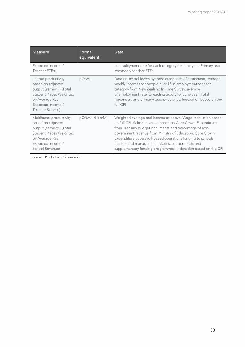
Working paper 2017/02
33
Measure Formal
equivalent
Data
Expected Income /
Teacher FTEs)
unemployment rate for each category for June year. Primary and
secondary teacher FTEs
Labour productivity
based on adjusted
output (earnings) (Total
Student Places Weighted
by Average Real
Expected Income /
Teacher Salaries)
pQ/wL Data on school levers by three categories of attainment, average
weekly incomes for people over 15 in employment for each
category from New Zealand Income Survey, average
unemployment rate for each category for June year. Total
(secondary and primary) teacher salaries. Indexation based on the
full CPI
Multifactor productivity
based on adjusted
output (earnings) (Total
Student Places Weighted
by Average Real
Expected Income /
School Revenue)
pQ/(wL+rK+mM) Weighted average real income as above. Wage indexation based
on full CPI. School revenue based on Core Crown Expenditure
from Treasury Budget documents and percentage of non-
government revenue from Ministry of Education. Core Crown
Expenditure covers roll-based operations funding to schools,
teacher and management salaries, support costs and
supplementary funding programmes. Indexation based on the CPI
Source: Productivity Commission
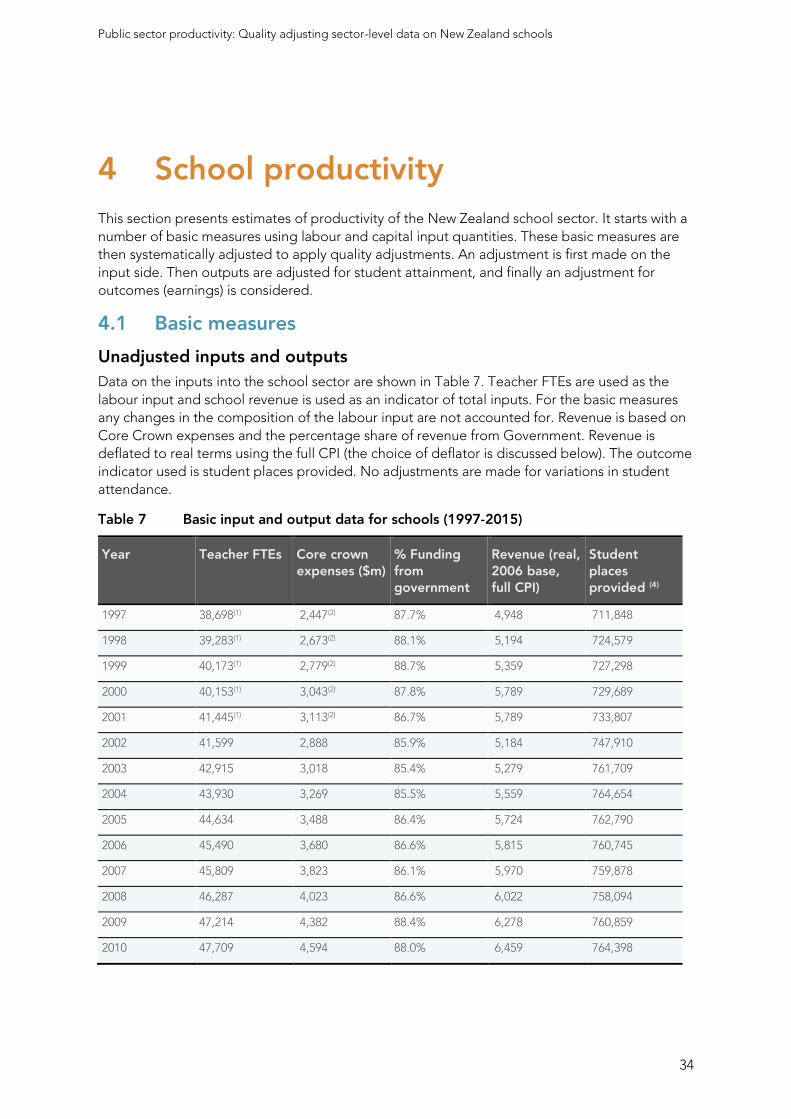
Public sector productivity: Quality adjusting sector-level data on New Zealand schools
34
4 School productivity
This section presents estimates of productivity of the New Zealand school sector. It starts with a
number of basic measures using labour and capital input quantities. These basic measures are
then systematically adjusted to apply quality adjustments. An adjustment is first made on the
input side. Then outputs are adjusted for student attainment, and finally an adjustment for
outcomes (earnings) is considered.
4.1 Basic measures
Unadjusted inputs and outputs
Data on the inputs into the school sector are shown in Table 7. Teacher FTEs are used as the
labour input and school revenue is used as an indicator of total inputs. For the basic measures
any changes in the composition of the labour input are not accounted for. Revenue is based on
Core Crown expenses and the percentage share of revenue from Government. Revenue is
deflated to real terms using the full CPI (the choice of deflator is discussed below). The outcome
indicator used is student places provided. No adjustments are made for variations in student
attendance.
Table 7 Basic input and output data for schools (1997-2015)
Year Teacher FTEs Core crown
expenses ($m)
% Funding
from
government
Revenue (real,
2006 base,
full CPI)
Student
places
provided (4)
1997 38,698(1) 2,447(2) 87.7% 4,948 711,848
1998 39,283(1) 2,673(2) 88.1% 5,194 724,579
1999 40,173(1) 2,779(2) 88.7% 5,359 727,298
2000 40,153(1) 3,043(2) 87.8% 5,789 729,689
2001 41,445(1) 3,113(2) 86.7% 5,789 733,807
2002 41,599 2,888 85.9% 5,184 747,910
2003 42,915 3,018 85.4% 5,279 761,709
2004 43,930 3,269 85.5% 5,559 764,654
2005 44,634 3,488 86.4% 5,724 762,790
2006 45,490 3,680 86.6% 5,815 760,745
2007 45,809 3,823 86.1% 5,970 759,878
2008 46,287 4,023 86.6% 6,022 758,094
2009 47,214 4,382 88.4% 6,278 760,859
2010 47,709 4,594 88.0% 6,459 764,398
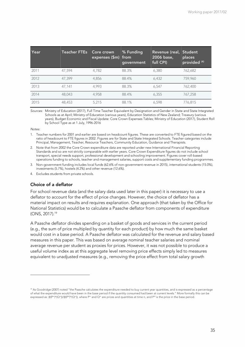
Working paper 2017/02
35
Year Teacher FTEs Core crown
expenses ($m)
% Funding
from
government
Revenue (real,
2006 base,
full CPI)
Student
places
provided (4)
2011 47,594 4,782 88.3% 6,380 762,682
2012 47,399 4,856 88.4% 6,432 759,960
2013 47,141 4,993 88.3% 6,547 762,400
2014 48,043 4,958 88.4% 6,355 767,258
2015 48,453 5,215 88.1% 6,598 776,815
Sources: Ministry of Education (2017), Full Time Teacher Equivalent by Designation and Gender in State and State Integrated Schools as at April; Ministry of Education (various years), Education Statistics of New Zealand; Treasury (various years), Budget Economic and Fiscal Update: Core Crown Expenses Tables; Ministry of Education (2017), Student Roll by School Type as at 1 July, 1996-2016
Notes:
1. Teacher numbers for 2001 and earlier are based on headcount figures. These are converted to FTE figured based on the ratio of headcount to FTE figures in 2002. Figures are for State and State Integrated Schools. Teacher categories include Principal, Management, Teacher, Resource Teachers, Community Education, Guidance and Therapists.
2. Note that from 2002 the Core Crown expenditure data are reported under new International Financial Reporting Standards and so are not strictly comparable with earlier years. Core Crown Expenditure figures do not include school transport, special needs support, professional development and schooling improvement. Figures cover roll-based operations funding to schools, teacher and management salaries, support costs and supplementary funding programmes.
3. Non-government funding includes local funds (62.6% of non-government revenue in 2015), international students (15.0%), investments (5.7%), hostels (4.2%) and other revenue (12.6%).
4. Excludes students from private schools.
Choice of a deflator
For school revenue data (and the salary data used later in this paper) it is necessary to use a
deflator to account for the effect of price changes. However, the choice of deflator has a
material impact on results and requires explanation. One approach (that taken by the Office for
National Statistics) would be to calculate a Paasche deflator from components of expenditure
(ONS, 2017).19
A Paasche deflator divides spending on a basket of goods and services in the current period
(e.g., the sum of price multipled by quantity for each product) by how much the same basket
would cost in a base period. A Paasche deflator was calculated for the revenue and salary based
measures in this paper. This was based on average nominal teacher salaries and nominal
average revenue per student as proxies for prices. However, it was not possible to produce a
useful volume index as at this aggregate level removing price effects simply led to measures
equivalent to unadjusted measures (e.g., removing the price effect from total salary growth
19 As Goodridge (2007) noted “the Paasche calculates the expenditure needed to buy current year quantities, and is expressed as a percentage
of what the expenditure would have been in the base period if the quantity consumed had been at current levels.” More formally this can be
expressed as: (Σ(Ptn)*(Qtn))/(Σ(Pt0)*(Qtn)), where Ptn and Qtn are prices and quantities at time n, and Pt0 is the price in the base period.
Public sector productivity: Quality adjusting sector-level data on New Zealand schools
36
resulted in an index equivalent to growth in teacher FTEs). This would require a more
disaggregated approach than that taken in this paper.
Nonetheless this showed that the average annual 4.4% increase in nominal total teacher salaries
reflected an average annual 3.2% increase in average teacher salaries and 1.2% increase in
teacher FTEs between 2002 and 2015. Likewise the average annual growth in nominal school
revenue was 4.4% between 2002 and 2015 (4.0% between 1997 and 2015), with a price effect of
4.2% (3.6% for the longer period) and an increase in student numbers of 0.3% (0.4% from 1997).
These figures can be compared with the growth in the CPI and the CPI level 2 subgroup for
primary and secondary education. This subgroup reflects consumers’ spending on schooling
and the CPI reflects price movements more generally. Between 2002 and 2015 the CPI grew by
an average of 2.2% (2.0% between 1997 and 2015) while the subgroup grew by an average of
5.2% (4.8% between 1997 and 2015).
Thus although nominal total teacher salaries grew at an annual average of 4.4%, this is less than
the annual average growth in the level 2 CPI subgroup (of 5.2%). The result is that if salaries are
deflated by the subgroup then real salaries will appear to have fallen, and productivity estimates
will be higher than otherwise. For instance using the subgroup as the deflator would mean:
Salary-based measures would grow faster than unadjusted productivity measures, even
though the growth in total salaries (4.4% nominal, or 2.1% real when deflated by the full CPI)
has been much faster than the growth in teacher FTEs (1.2%) or price growth more generally
(the CPI at 2.2%). (To illustrate Appendix A contains a summary of the measures in this paper
using the subgroup as a deflator.) Higher salary growth should (all else being constant) lead
to lower productivity growth so the results of these two measures would be inconsistent.
Similar issues arise in relation to school revenue, where nominal school revenue (average
annual growth of 4.0% between 1997 and 2015) has risen much faster than student numbers
(average annual growth of 0.4% for the same period).
Consequently the full CPI is used to deflate teacher salaries and school revenue in this paper.20
The full CPI provides a “common numeraire” as the basis for all real comparisons – so it
indicates a common average real basket of goods that the funds in question cold alternatively
buy. Nonetheless, the sensitivity of final productivity comparisons to the deflator choice is a
reason for caution in interpreting schools’ productivity trends.
Results
The change in these basic inputs and outputs are shown in two measures in Figure 6. This plots
the pupil-staff ratio in the school sector and the real revenue per pupil from 1997 to 2015.
Further, along with an increase in staff members per student the cost per student (when indexed
20 Another possible deflator is the education and training subgroup of Statistics New Zealand’s Purchasing Price Index (PPI). Yet this index only
covers the “productive sector” and measures changes in the prices of outputs that generate operating income and inputs that incur operating
expense. It does not include prices for items related to capitalised expenditure, non-operating income, financing costs, or employee
compensation. The education and training subgroup is not published at a further disaggregated level (e.g., for primary and secondary schools).
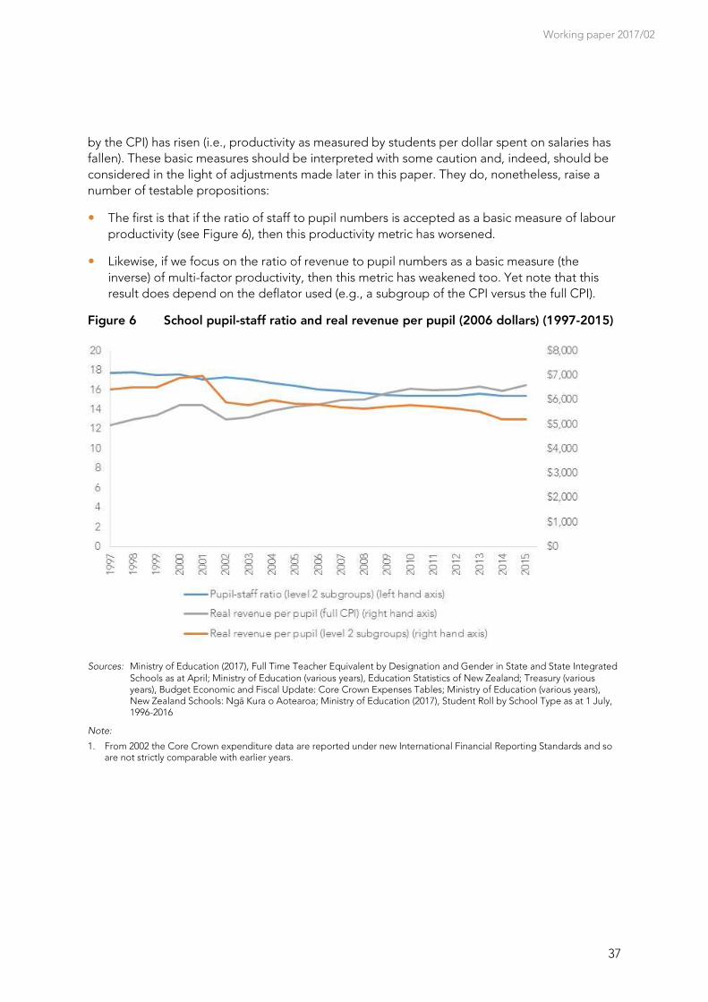
Working paper 2017/02
37
by the CPI) has risen (i.e., productivity as measured by students per dollar spent on salaries has
fallen). These basic measures should be interpreted with some caution and, indeed, should be
considered in the light of adjustments made later in this paper. They do, nonetheless, raise a
number of testable propositions:
The first is that if the ratio of staff to pupil numbers is accepted as a basic measure of labour
productivity (see Figure 6), then this productivity metric has worsened.
Likewise, if we focus on the ratio of revenue to pupil numbers as a basic measure (the
inverse) of multi-factor productivity, then this metric has weakened too. Yet note that this
result does depend on the deflator used (e.g., a subgroup of the CPI versus the full CPI).
Figure 6 School pupil-staff ratio and real revenue per pupil (2006 dollars) (1997-2015)
Sources: Ministry of Education (2017), Full Time Teacher Equivalent by Designation and Gender in State and State Integrated Schools as at April; Ministry of Education (various years), Education Statistics of New Zealand; Treasury (various years), Budget Economic and Fiscal Update: Core Crown Expenses Tables; Ministry of Education (various years), New Zealand Schools: Ngā Kura o Aotearoa; Ministry of Education (2017), Student Roll by School Type as at 1 July, 1996-2016
Note:
1. From 2002 the Core Crown expenditure data are reported under new International Financial Reporting Standards and so are not strictly comparable with earlier years.
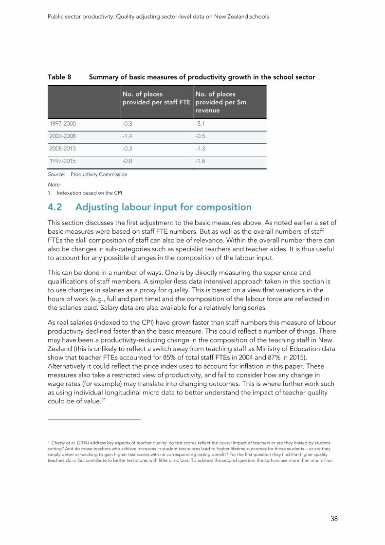
Public sector productivity: Quality adjusting sector-level data on New Zealand schools
38
Table 8 Summary of basic measures of productivity growth in the school sector
No. of places
provided per staff FTE
No. of places
provided per $m
revenue
1997-2000 -0.3 -5.1
2000-2008 -1.4 -0.5
2008-2015 -0.3 -1.3
1997-2015 -0.8 -1.6
Source: Productivity Commission
Note:
1. Indexation based on the CPI.
4.2 Adjusting labour input for composition
This section discusses the first adjustment to the basic measures above. As noted earlier a set of
basic measures were based on staff FTE numbers. But as well as the overall numbers of staff
FTEs the skill composition of staff can also be of relevance. Within the overall number there can
also be changes in sub-categories such as specialist teachers and teacher aides. It is thus useful
to account for any possible changes in the composition of the labour input.
This can be done in a number of ways. One is by directly measuring the experience and
qualifications of staff members. A simpler (less data intensive) approach taken in this section is
to use changes in salaries as a proxy for quality. This is based on a view that variations in the
hours of work (e.g., full and part time) and the composition of the labour force are reflected in
the salaries paid. Salary data are also available for a relatively long series.
As real salaries (indexed to the CPI) have grown faster than staff numbers this measure of labour
productivity declined faster than the basic measure. This could reflect a number of things. There
may have been a productivity-reducing change in the composition of the teaching staff in New
Zealand (this is unlikely to reflect a switch away from teaching staff as Ministry of Education data
show that teacher FTEs accounted for 85% of total staff FTEs in 2004 and 87% in 2015).
Alternatively it could reflect the price index used to account for inflation in this paper. These
measures also take a restricted view of productivity, and fail to consider how any change in
wage rates (for example) may translate into changing outcomes. This is where further work such
as using individual longitudinal micro data to better understand the impact of teacher quality
could be of value.21
21 Chetty et al. (2014) address key aspects of teacher quality: do test scores reflect the causal impact of teachers or are they biased by student
sorting? And do those teachers who achieve increases in student test scores lead to higher lifetime outcomes for those students – or are they
simply better at teaching to gain higher test scores with no corresponding lasting benefit? For the first question they find that higher quality
teachers do in fact contribute to better test scores with little or no bias. To address the second question the authors use more than one million
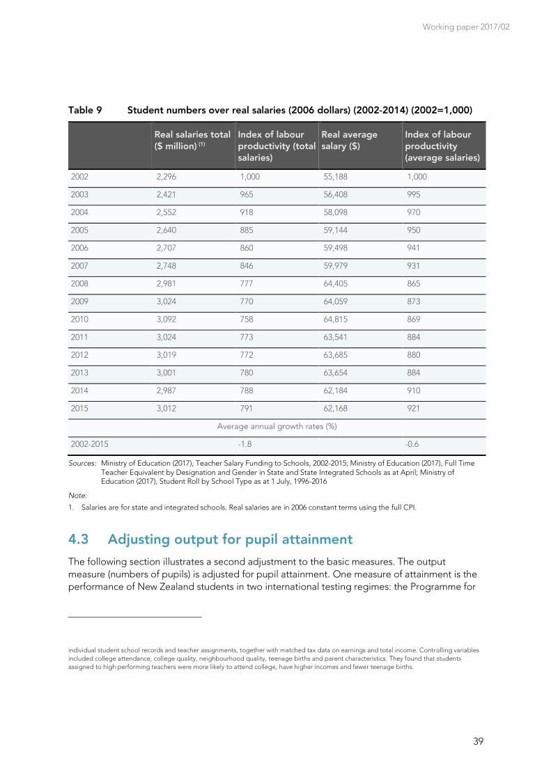
Working paper 2017/02
39
Table 9 Student numbers over real salaries (2006 dollars) (2002-2014) (2002=1,000)
Real salaries total
($ million) (1)
Index of labour
productivity (total
salaries)
Real average
salary ($)
Index of labour
productivity
(average salaries)
2002 2,296 1,000 55,188 1,000
2003 2,421 965 56,408 995
2004 2,552 918 58,098 970
2005 2,640 885 59,144 950
2006 2,707 860 59,498 941
2007 2,748 846 59,979 931
2008 2,981 777 64,405 865
2009 3,024 770 64,059 873
2010 3,092 758 64,815 869
2011 3,024 773 63,541 884
2012 3,019 772 63,685 880
2013 3,001 780 63,654 884
2014 2,987 788 62,184 910
2015 3,012 791 62,168 921
Average annual growth rates (%)
2002-2015 -1.8 -0.6
Sources: Ministry of Education (2017), Teacher Salary Funding to Schools, 2002-2015; Ministry of Education (2017), Full Time Teacher Equivalent by Designation and Gender in State and State Integrated Schools as at April; Ministry of Education (2017), Student Roll by School Type as at 1 July, 1996-2016
Note:
1. Salaries are for state and integrated schools. Real salaries are in 2006 constant terms using the full CPI.
4.3 Adjusting output for pupil attainment
The following section illustrates a second adjustment to the basic measures. The output
measure (numbers of pupils) is adjusted for pupil attainment. One measure of attainment is the
performance of New Zealand students in two international testing regimes: the Programme for
individual student school records and teacher assignments, together with matched tax data on earnings and total income. Controlling variables
included college attendance, college quality, neighbourhood quality, teenage births and parent characteristics. They found that students
assigned to high performing teachers were more likely to attend college, have higher incomes and fewer teenage births.
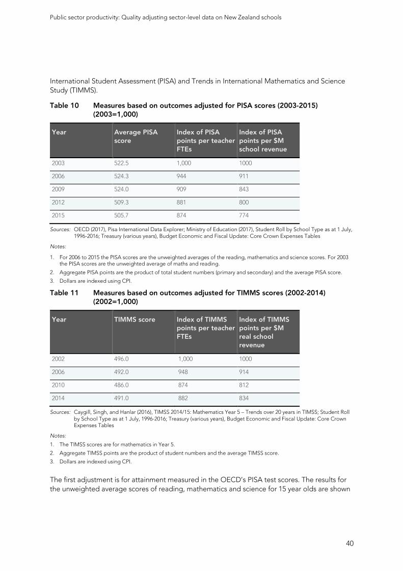
Public sector productivity: Quality adjusting sector-level data on New Zealand schools
40
International Student Assessment (PISA) and Trends in International Mathematics and Science
Study (TIMMS).
Table 10 Measures based on outcomes adjusted for PISA scores (2003-2015) (2003=1,000)
Year Average PISA
score
Index of PISA
points per teacher
FTEs
Index of PISA
points per $M
school revenue
2003 522.5 1,000 1000
2006 524.3 944 911
2009 524.0 909 843
2012 509.3 881 800
2015 505.7 874 774
Sources: OECD (2017), Pisa International Data Explorer; Ministry of Education (2017), Student Roll by School Type as at 1 July, 1996-2016; Treasury (various years), Budget Economic and Fiscal Update: Core Crown Expenses Tables
Notes:
1. For 2006 to 2015 the PISA scores are the unweighted averages of the reading, mathematics and science scores. For 2003 the PISA scores are the unweighted average of maths and reading.
2. Aggregate PISA points are the product of total student numbers (primary and secondary) and the average PISA score.
3. Dollars are indexed using CPI.
Table 11 Measures based on outcomes adjusted for TIMMS scores (2002-2014) (2002=1,000)
Year TIMMS score Index of TIMMS
points per teacher
FTEs
Index of TIMMS
points per $M
real school
revenue
2002 496.0 1,000 1000
2006 492.0 948 914
2010 486.0 874 812
2014 491.0 882 834
Sources: Caygill, Singh, and Hanlar (2016), TIMSS 2014/15: Mathematics Year 5 – Trends over 20 years in TIMSS; Student Roll by School Type as at 1 July, 1996-2016; Treasury (various years), Budget Economic and Fiscal Update: Core Crown Expenses Tables
Notes:
1. The TIMSS scores are for mathematics in Year 5.
2. Aggregate TIMSS points are the product of student numbers and the average TIMSS score.
3. Dollars are indexed using CPI.
The first adjustment is for attainment measured in the OECD’s PISA test scores. The results for
the unweighted average scores of reading, mathematics and science for 15 year olds are shown

Working paper 2017/02
41
in Table 10 for every year for which the testing was administered. The scores have been used to
form an aggregate number of student PISA points (multiplying the average score by the total
number of student places), which provides an adjusted measure of output. The decline in the
average PISA score (an average annual decline of 0.3%) is larger than the decline in aggregate
PISA points (an average annual decline of 0.1%) as the number of students has increased slightly
(an average annual increase of 0.2%) over the period. The ratio of this adjusted output can be
divided by inputs (teacher FTEs and school revenue) as indicators of labour and multi-factor
productivity respectively. These ratios, along with changes in their index levels (where the 2003
level is equal to 1,000), are shown in Table 10.
A similar exercise can be repeated with the TIMMS data. The TIMMS scores refer to the average
score for mathematics in Year 5 and so are based on performance at primary school. The
aggregate student TIMMS points is, as with PISA-based adjustments, based on the average
TIMMS score multiplied by the total number of student places. The ratio of this adjusted output
to two inputs (staff FTEs) and (revenue) can then be calculated as indicators of labour and multi-
factor productivity. These ratios, along with changes in their index levels (where the 2002 level is
equal to 1,000), are shown in Table 11.
There are several important caveats to bear in mind when using attainment measures like test
scores to adjust outputs. In particular:
The PISA and TIMMs attainment scores are used to adjust total school education output, but
these indicators relate to specific elements within the school education system. They may
not be representative of attainment across the broader school curriculum or pupil age
ranges.
There is the issue of attribution. In particular, how much of the attainment is due to the
education system, rather than characteristics of the student’s background, upbringing,
parental engagement, early childhood nutrition, neighbourhood, etc. Indeed, the OECD has
estimated that almost 20 percent of the variance in the 2012 PISA mathematics scores for
New Zealand can be explained by the students’ socio-economic background. This is one of
the highest levels in the OECD (OECD, 2014).
A related issue is the inherent quality of the student intake. There are also questions of
timing, as the attainment in a test at, say, age 15 reflects not only the learning in the current
year but the cumulative effect of the learning acquired throughout previous years of
schooling.
Further, while both the PISA and TIMMs test scores provide a useful picture on overall
student attainment, they cannot illustrate the progress that individual students make from
one assessment to the next. Tracking performance in this way would provide a measure of
value add (Jensen, 2010).
It could be possible to disentangle some of these issues through the use of micro-data, such as
New Zealand’s Integrated Data Infrastructure (IDI).
Public sector productivity: Quality adjusting sector-level data on New Zealand schools
42
4.4 Adjusting for outcomes (earnings)
A further adjustment is to account for the possible impact of education on key outcomes, such
as earnings. This human capital approach to assessing the contribution of education has been
widely used. It is based on a view that output of the education system adds to an individual’s
stock of human capital (Jorgenson and Fraumeni,1992), and has been used in studies of the
returns to education (e.g., Maani and Maloney, 2004) and to adjust for quality (e.g., O’Mahony
and Stevens, 2009). At the same time there are a number of potential drawbacks of this
approach (e.g., Hanushek, 2015; Burgess, 2016).
As in the case of student attainment, it is important to recognise that outcomes such as earnings
reflect more than just the education system (e.g., labour market conditions, technological
change, and learning in other environments). There may also be a selection bias where students
with favourable backgrounds are likely to elect to gain additional qualifications and to be
successful in the labour market (Schreyer, 2010). And the school system influences a wide range
of outcomes beyond earnings, both for the individual and for society more generally.
Nevertheless, a benefit of using earnings as an outcome measure is that it can be seen as a
proxy for a price in a market, and so creates some comparability with productivity measurement in the measured sector. A measure of future real earnings also recognises that the real return to
a given student’s education may change over time.
The adjustments made in this section follow an OECD approach developed by Murray (2007)
and applied to Scotland. This involved two stages:
First, school leavers were separated into three attainment categories. The categories are
shown in Table 12. Note that as the school attainment measures have evolved over time the
definitions of the categories have also changed. The goal has been to develop categories
that provide broadly consistent measures of performance across all of the years studied.
(This measure of domestic attainment is used as the output measure in the comparison with
the Office for National Statistics approach (discussed in section 5).)
Second, for each of the three categories the average weekly income (earnings plus transfers)
for wage and salary earners 15 years of age and older were drawn from the New Zealand
Income Survey. These were converted to an expected real income by adjusting for
unemployment rates and inflation (the full CPI). A detailed breakdown of the data for each of
the three attainment categories is given in Table B.1 in Appendix A. The average weekly
income was multiplied by the employment rate (one minus the unemployment rate) to give
an adjusted income. The average real expected income for each category was then
multiplied by the number of people in that category to give an attainment weighted real
income total. This income measure forms the output measure for the productivity
calculations.
There are a number of important caveats to bear in mind with these estimates. The results apply
to people with wage or salary income or who are self-employed, i.e., they do not cover people
not in the labour force. Furthermore, it is assumed that previous levels of income are a good
indicator of levels of income in the future. Further, these results are partly driven by the increase
in the proportion of students leaving school with NCEA level 2 (or equivalent) or above
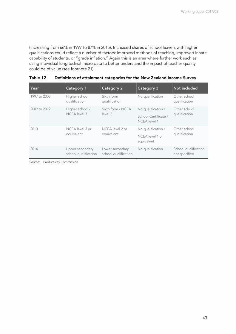
Working paper 2017/02
43
(increasing from 66% in 1997 to 87% in 2015). Increased shares of school leavers with higher
qualifications could reflect a number of factors: improved methods of teaching, improved innate
capability of students, or “grade inflation.” Again this is an area where further work such as
using individual longitudinal micro data to better understand the impact of teacher quality
could be of value (see footnote 21).
Table 12 Definitions of attainment categories for the New Zealand Income Survey
Year Category 1 Category 2 Category 3 Not included
1997 to 2008 Higher school
qualification
Sixth form
qualification
No qualification Other school
qualification
2009 to 2012 Higher school /
NCEA level 3
Sixth form / NCEA
level 2
No qualification /
School Certificate /
NCEA level 1
Other school
qualification
2013 NCEA level 3 or
equivalent
NCEA level 2 or
equivalent
No qualification /
NCEA level 1 or
equivalent
Other school
qualification
2014 Upper secondary
school qualification
Lower secondary
school qualification
No qualification School qualification
not specified
Source: Productivity Commission
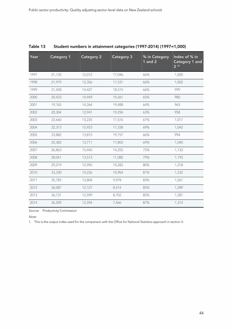
Public sector productivity: Quality adjusting sector-level data on New Zealand schools
44
Table 13 Student numbers in attainment categories (1997-2014) (1997=1,000)
Year Category 1 Category 2 Category 3 % in Category
1 and 2
Index of % in
Category 1 and
2 (1)
1997 21,135 12,012 17,046 66% 1,000
1998 21,979 12,356 17,531 66% 1,002
1999 21,458 14,427 18,515 66% 999
2000 20,423 14,949 19,261 65% 980
2001 19,765 14,264 19,488 64% 963
2002 20,304 12,941 19,296 63% 958
2003 22,660 13,235 17,576 67% 1,017
2004 22,373 15,923 17,338 69% 1,042
2005 23,882 13,815 19,757 66% 994
2006 25,382 13,711 17,802 69% 1,040
2007 26,863 15,445 14,255 75% 1,133
2008 28,041 13,513 11,080 79% 1,195
2009 29,219 12,992 10,282 80% 1,218
2010 33,330 14,226 10,904 81% 1,232
2011 35,783 13,804 9,978 83% 1,261
2012 36,087 12,127 8,414 85% 1,289
2013 36,731 12,599 8,702 85% 1,287
2014 36,509 12,594 7,466 87% 1,314
Source: Productivity Commission
Note:
1. This is the output index used for the comparison with the Office for National Statistics approach in section 5.
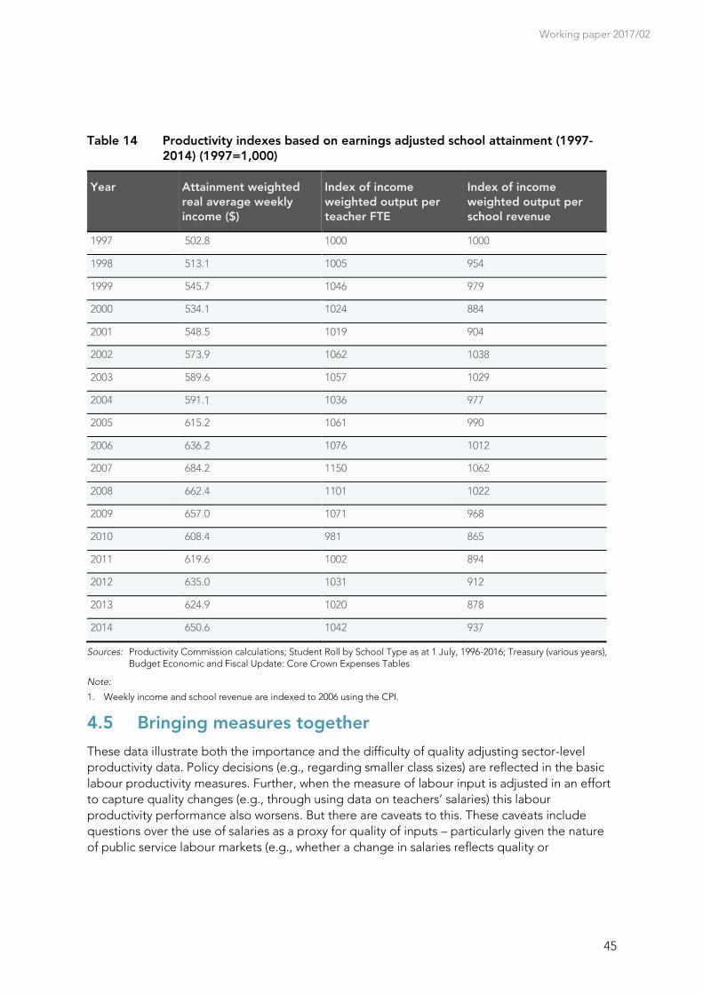
Working paper 2017/02
45
Table 14 Productivity indexes based on earnings adjusted school attainment (1997-2014) (1997=1,000)
Year Attainment weighted
real average weekly
income ($)
Index of income
weighted output per
teacher FTE
Index of income
weighted output per
school revenue
1997 502.8 1000 1000
1998 513.1 1005 954
1999 545.7 1046 979
2000 534.1 1024 884
2001 548.5 1019 904
2002 573.9 1062 1038
2003 589.6 1057 1029
2004 591.1 1036 977
2005 615.2 1061 990
2006 636.2 1076 1012
2007 684.2 1150 1062
2008 662.4 1101 1022
2009 657.0 1071 968
2010 608.4 981 865
2011 619.6 1002 894
2012 635.0 1031 912
2013 624.9 1020 878
2014 650.6 1042 937
Sources: Productivity Commission calculations; Student Roll by School Type as at 1 July, 1996-2016; Treasury (various years), Budget Economic and Fiscal Update: Core Crown Expenses Tables
Note:
1. Weekly income and school revenue are indexed to 2006 using the CPI.
4.5 Bringing measures together
These data illustrate both the importance and the difficulty of quality adjusting sector-level
productivity data. Policy decisions (e.g., regarding smaller class sizes) are reflected in the basic
labour productivity measures. Further, when the measure of labour input is adjusted in an effort
to capture quality changes (e.g., through using data on teachers’ salaries) this labour
productivity performance also worsens. But there are caveats to this. These caveats include
questions over the use of salaries as a proxy for quality of inputs – particularly given the nature
of public service labour markets (e.g., whether a change in salaries reflects quality or

Public sector productivity: Quality adjusting sector-level data on New Zealand schools
46
compositional changes) and the importance of missing inputs such as the previous performance
of students (needed for measures of value added).
Table 15 Summary of measures (CPI deflator)
Year Q/L Q/wL pQ/L(1) pQ/L(2) pQ/wL Q/(wL+rK+
mM)
pQ/(wL+rK+
mM)
2002 1,000 1,000 1,000 1,000 1,000 1,000
2003 986 965 1,000 996 974 982 992
2004 967 918 975 927 933 941
2005 949 885 999 933 906 954
2006 928 860 944 1,014 941 892 975
2007 919 846 1,083 996 868 1,023
2008 907 777 1,037 889 861 985
2009 893 770 909 1,009 869 826 933
2010 890 758 924 787 803 834
2011 890 773 944 820 813 862
2012 891 772 881 971 842 806 879
2013 899 780 961 833 792 846
2014 888 788 982 871 816 902
2015 891 791 874 786
Average Annual Growth Rates
2002-2008 -1.6% -4.1% 0.6% -1.9% -2.5% -0.3%
2008-2014 -0.4% 0.2% -0.9% -0.3% -0.9% -1.4%
2002-2014 -1.0% -2.0% -1.1% -0.2% -1.1% -1.7% -0.9%
Source: Productivity Commission
Notes:
1. Two other measures based on domestic attainment (with no adjustment for expected real wages) are shown in Table 16.
2. Q/L equals student numbers/teacher FTEs.
3. Q/wL equals student numbers/teacher salaries.
4. pQ/L(1) equals student numbers weighted by attainment in PISA scores/teacher FTEs.
5. pQ/L(2) equals income weighted output/teacher FTEs.
6. pQ/wL equals income weighted output/teacher salaries.
7. Q/(wL+rK+mM) equals student numbers/school revenue.
8. pQ/(wL+rK+mM) equals income weighted output/school revenue.
Working paper 2017/02
47
Nonetheless, a similar story emerges from measures that adjust outputs based on attainment in
international assessments (such as New Zealand students’ PISA scores), where performance has
worsened. This reflects a decline in aggregate PISA points (an average annual decline of 0.1%),
which itself reflects a larger fall in the average PISA score (an average annual decline of 0.3%).
However, there are differences in measured attainment according to international and domestic
assessments. Indeed, (labour) productivity based on a measure that adjusted for domestic
attainment (e.g., the proportion of students leaving school with NCEA level 2 (or equivalent))
increased between 2002 and 2014. A related measure (the series using school revenue as a
measure of inputs) was used to compare the results in this paper to those of the Office for
National Statistics in the United Kingdom.
Finally, measures were adjusted for final outcomes (in this case the performance of school
leavers in the labour market). This involved a two-step process:
First, output was adjusted for the domestic attainment of students.
The average real expected income for students based on this attainment was then
estimated and multiplied by the number of students in each category.
These measures also suggested falling productivity. But these measures can be subject to
attribution problems. Indeed, given the improved domestic attainment above, the decline in
these measures reflected changes in unemployment and real wage growth following the Global
Financial Crisis. With the use of sector-level data it is thus not possible to conclude that changes
in these measures are directly attributable to the performance of schools, e.g., they may also
reflect differences in the economic context facing different cohorts of school leavers. To
estimate the incremental value of school education on earnings it would be necessary to use
linked unit record data.
Public sector productivity: Quality adjusting sector-level data on New Zealand schools
48
5 Comparison with ONS estimates of education productivity
This section compares some of the results in this paper against a similar series produced by the
Office for National Statistics (ONS) in the United Kingdom. As discussed the ONS has been at
the forefront of developments in measuring public sector productivity and so a comparison of
approaches could be instructive.
In the United Kingdom output is based on the numbers of students adjusted for absences. This
is quality adjusted for the Level 2 attainment by students in England, a five year geometric
average of average point scores for students at this level in Scotland, and average point scores
for GCSEs in Wales. Student numbers are adjusted based on the average point scores in these
exams. As discussed in footnote 3, the ONS has had to revise its approach to quality adjusting
education quantity when practices regarding students sitting exams changed.
In New Zealand output (numbers of primary and secondary students, not accounting for
absences) is adjusted based on the proportion of students completing schooling with NCEA
level 2 (or earlier equivalent) or more. In relation to input measures used, in New Zealand school
revenue is used as the input measure. In the United Kingdom, inputs include labour, goods and
services, and consumption of fixed capital, which are all weighted by expenditure share.
It is important to recognise that given differences in public policies, policy contexts, and data
availability it is appropriate for there to be some small methodological differences in the two
approaches. Findings can thus be expected to differ. Yet similarities in the general magnitude
and direction of effect from making broadly similar quality adjustment (based on performance in
domestic assessments) could be expected.
The results in Figure 7 show that in both countries the unadjusted series show a downward shift
over time, reflecting policy choices for smaller class sizes. But in both cases making a quality
adjustment based on pupil attainment leads to improved (lower rate of decline in) productivity.
In New Zealand the average unadjusted annual productivity growth for 1997 to 2014 was -2.1%,
while in the United Kingdom it was -1.6%. In contrast, the average adjusted productivity growth
over this period was -0.5% in New Zealand and -0.2% in the United Kingdom. However, a higher
proportion of students achieving NCEA level 2 or above (or equivalent) in New Zealand has
been reflected in strong multifactor productivity growth for the adjusted series since 2005.
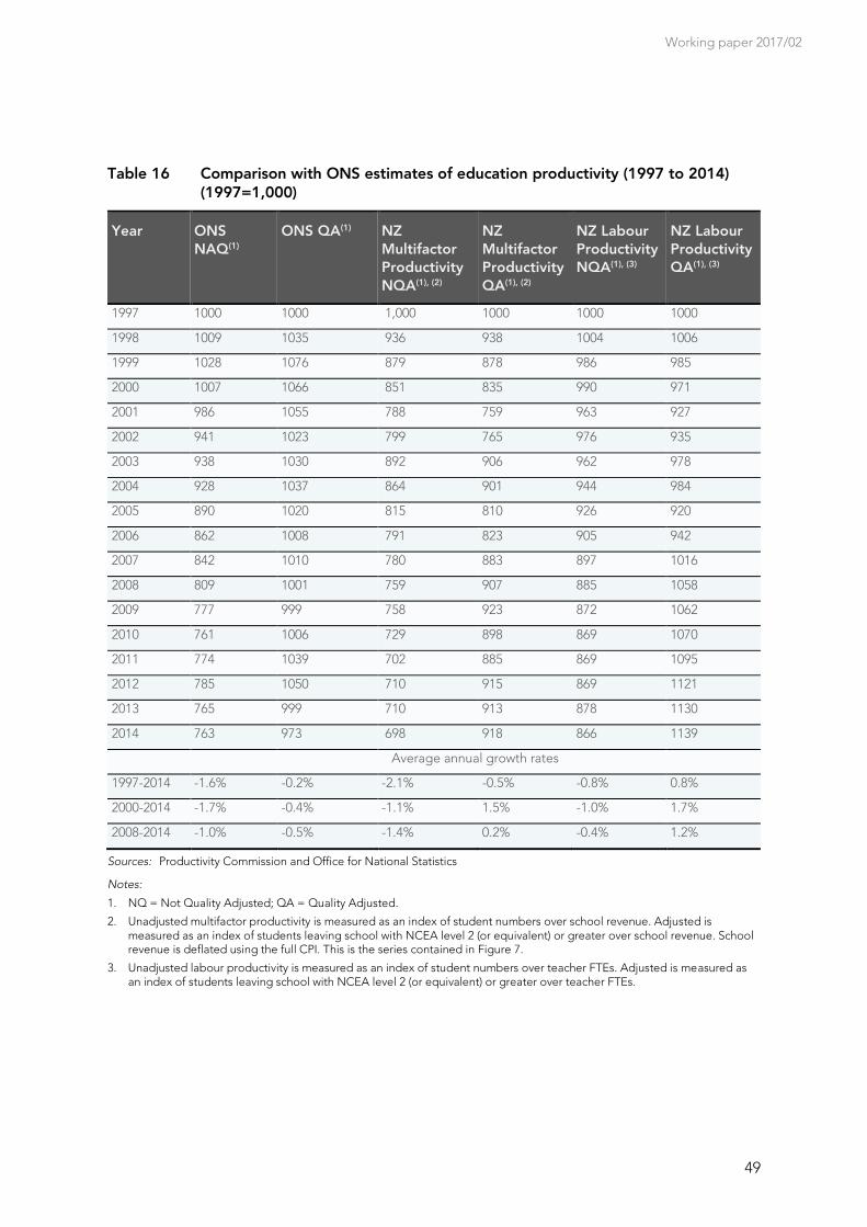
Working paper 2017/02
49
Table 16 Comparison with ONS estimates of education productivity (1997 to 2014) (1997=1,000)
Year ONS
NAQ(1)
ONS QA(1) NZ
Multifactor
Productivity
NQA(1), (2)
NZ
Multifactor
Productivity
QA(1), (2)
NZ Labour
Productivity
NQA(1), (3)
NZ Labour
Productivity
QA(1), (3)
1997 1000 1000 1,000 1000 1000 1000
1998 1009 1035 936 938 1004 1006
1999 1028 1076 879 878 986 985
2000 1007 1066 851 835 990 971
2001 986 1055 788 759 963 927
2002 941 1023 799 765 976 935
2003 938 1030 892 906 962 978
2004 928 1037 864 901 944 984
2005 890 1020 815 810 926 920
2006 862 1008 791 823 905 942
2007 842 1010 780 883 897 1016
2008 809 1001 759 907 885 1058
2009 777 999 758 923 872 1062
2010 761 1006 729 898 869 1070
2011 774 1039 702 885 869 1095
2012 785 1050 710 915 869 1121
2013 765 999 710 913 878 1130
2014 763 973 698 918 866 1139
Average annual growth rates
1997-2014 -1.6% -0.2% -2.1% -0.5% -0.8% 0.8%
2000-2014 -1.7% -0.4% -1.1% 1.5% -1.0% 1.7%
2008-2014 -1.0% -0.5% -1.4% 0.2% -0.4% 1.2%
Sources: Productivity Commission and Office for National Statistics
Notes:
1. NQ = Not Quality Adjusted; QA = Quality Adjusted.
2. Unadjusted multifactor productivity is measured as an index of student numbers over school revenue. Adjusted is measured as an index of students leaving school with NCEA level 2 (or equivalent) or greater over school revenue. School revenue is deflated using the full CPI. This is the series contained in Figure 7.
3. Unadjusted labour productivity is measured as an index of student numbers over teacher FTEs. Adjusted is measured as an index of students leaving school with NCEA level 2 (or equivalent) or greater over teacher FTEs.
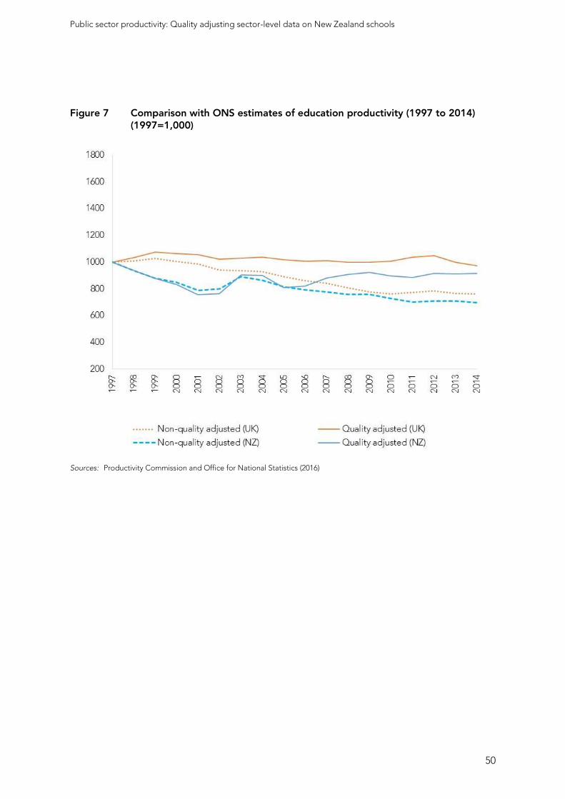
Public sector productivity: Quality adjusting sector-level data on New Zealand schools
50
Figure 7 Comparison with ONS estimates of education productivity (1997 to 2014) (1997=1,000)
Sources: Productivity Commission and Office for National Statistics (2016)
Working paper 2017/02
51
6 References
Abbott, M. & Doucouliagos, C. (2002). Technical and scale efficiency of vocational education
and training institutions: The case of the New Zealand polytechnics. New Zealand
Economic Papers, 34(1):1-23.
Abbott, M. & Doucouliagos, C. (2009). Competition and efficiency: overseas students and technical efficiency in Australian and New Zealand universities. Education Economics,
17(1):31-57.
Afonso, A. (2009). Quality of public finances: some illustrations. Presentation to a European
Central Bank workshop on Politica fiscal y coordinacion de politicas. San Sebastian, 24
July.
Afonso, A. & St. Aubyn, M. (2005). Non-parametric approaches to education and health efficiency in OECD countries. Journal of Applied Economics, 8(2):227-246.
Afonso, A. & St. Aubyn, M. (2006). Cross-country efficiency of secondary education provision: A semi-parametric analysis with non-discretionary inputs. Economic Modelling, 23: 476-91.
Alexander, W. & Jaforullah, M. (2005). Scale and pure efficiencies of New Zealand secondary
schools. Economics Discussion Papers No. 0501, University of Otago.
Alexander, W, Haug, A. & Jaforullah, M. (2007). A two-stage double-bootstrap data
envelopment analysis of efficiency differences of New Zealand secondary schools.
Economics Discussion Papers No. 0714, University of Otago.
Arndt, C & Oman, C. (2006). Uses and Abuses of Government Indicators. Development Centre
Studies, Paris, France: OECD.
Atkinson. A. (2005a). Measurement of government output and productivity for the national
accounts. New York: Palgrave Macmillan.
Atkinson. A. (2005b) Measurement of UK government output and productivity for the national accounts. Journal of the Statistical and Social Inquiry Society of Ireland, 34: 152-160.
Audit Office of Victoria (2013). Performance reporting systems in education. PP No. 263, Session
2010-13. Retrieved from www.audit.vic.gov.au/publications/20130918-Performance-
reporting/20130918-Performance-
Baker, B. & Kelly, P. (2008). A primer on the BEA’s government accounts. BEA Briefing.
Washington, DC: Bureau of Economic Analysis
Barslund, M. & O’Mahony, M. (2012). Output and productivity in the education sector. Indicators
for Evaluating International Performance in Service Sectors (INDICSER). Discussion Paper
39, Research Directorate General, European Commission, Brussels.
Public sector productivity: Quality adjusting sector-level data on New Zealand schools
52
Baumol, W. & Bowen, W. (1966). Performing Arts, The Economic Dilemma: a study of problems
common to theatre, opera, music, and dance. New York: Twentieth Century Fund.
Bean, C. (2016). Independent review of UK economic statistics: final report. HM Treasury,
London. Retrieved from https://www.gov.uk/government/publications/independent-
review-of-uk-economic-statistics-final-report
Black, S. (1998). Measuring the value of better schools. Federal Reserve Bank of New York. Economic Policy Review, 4(1):87-94.
Blundell, R., Dearden, L. & Sianesi, B. (2004). Evaluating the impact of education on earnings in
the UK: Models, methods and results from the NCDS. Working Paper WP03/20. The
Institute for Fiscal Studies, London.
Bouckaert, G. & van de Walle, S. (2003). Comparing measures of citizen trust and user
satisfaction as indicators of ‘good governance’: difficulties in linking trust and satisfaction.
International Review of Administrative Sciences, 69(3): 329-343.
Bowles, S., Gintis, H. & Osborne, M. (2001). The Determinants of Earnings: A Behavioral Approach. Journal of Economic Literature, 9(4):1137-1176.
Boyle, R. (2007). Public sector productivity measurement: an impossible task? In Aylward, C. &
O'Toole, R. (Eds.) (2007). Perspectives on Irish Productivity. Dublin: Forfas.
Bridge, M. (2015). ‘Methods change in public service productivity estimates: education 2013,’
Information Note, Office for National Statistics, London.
Burgess, S. (2016). Human capital and education: The state of the art in the economics of
education. Discussion Paper No. 9885, Institute for the Study of Labour (IZA), Bonn.
Cannon, S, Danielsen, B. and Harrison, D. (2015). School vouchers and home prices: Premiums in school districts lacking public schools. Journal of Housing Research, 24(1):1-20.
Caul, S. (2014). Public service productivity estimates: Education 2012. UK Office for National
Statistics.
Chetty, R., Friedman, J. & Rockoff, J. (2014). Measuring the impacts of teachers I: Evaluating bias
in teacher value-added estimates. American Economic Review, 104(9):2593-2632.
Christian, M. & Fraumeni, B. (2005). Measuring the education function of government.
Washington, DC: Bureau of Economic Analysis.
Coelli, T. (1995). Recent developments in frontier modelling and efficiency measurement. Australian. Journal of Agricultural Economics, 39(3):219-245.
Coelli, T. (2002). A comparison of alternative productivity growth measures: with application to electricity generation. In K. J. Fox (ed.) Efficiency in the Public Sector. Boston: Kluwer
Academic Publishers.
Coelli, T., Prasad Rao, D., & O’Donnell, C. (2005). Productivity Analysis. New York: Springer.
Working paper 2017/02
53
Coleman, J. et al. (1966). Equality of Educational Opportunity. Office of Education, US
Department of Health, Education and Welfare, Washington, DC.
Collesi, D., Guerrucci, D., Versace, D., & Zannoni, S. (2007). The use of class size and the Italian
method. Workshop on measuring Education and Health Volume. National Accounts and
Financial Statistics Division, OECD: Paris. Retrieved from
www.oecd.org/std/na/38685528.pdf
Conway, P. (2016). Achieving New Zealand’s productivity potential. New Zealand Productivity
Commission, Wellington.
Conway, P. & Meehan, L. (2013). Productivity by the numbers: The New Zealand experience.
Research Paper 2013/01, New Zealand Productivity Commission, Wellington.
Crowhurst, E., Finch. A. & Harwich, E. (2015). Toward a more productive state. Reform, London.
Retrieved from www.reform.uk/wp-content/uploads/2015/11/Productive-
state_AW_FINAL.pdf
Curristine, T., Lonti, Z. & Journard, I. (2007). Improving public sector efficiency: challenges and
opportunities. OECD Journal on Budgeting 7(1):161-201.
Daraio, C. & Simar, L. (2005). Introducing Environmental Variables in Nonparametric Frontier
Models: a Probabilistic Approach. Journal of Productivity Analysis, 24:93–121.
Department of Education and Skills (2005). Measuring Government Education Output in the
National Accounts: An Overview of Several Methods Developed as Part of the Atkinson
Review.
Djellal, F. & Gallouj, F. (2008). Measuring and improving productivity in services: Issues,
strategies and challenges. Cheltenham: Edward Elgar Publishing Ltd.
Dutu, R. & Sicari, P. (2016). Public Spending Efficiency in the OECD: Benchmarking Health Care,
Education and General Administration. OECD Economics Department Working Papers,
No. 1278, Paris: OECD. Retrieved from http://dx.doi.org/10.1787/5jm3st732jnq-en
Dunleavy, P. (2016). Public Sector Productivity: Measurement challenges, performance
information and prospects for improvement. OECD: Paris
Eurostat (2001) Handbook on price and volume measures in national accounts. European
Commission, Luxembourg. Retrieved from
http://ec.europa.eu/eurostat/documents/3859598/5827257/KS-41-01-543-
EN.PDF/10be98a9-083d-446a-a528-682c95914e9f
Francis, D. & Horn, M. (2013). Core Guide 3: Getting to Great; Lead Reviewer insights from the
Performance Improvement Framework. State Services Commission, the Treasury and the
Department of the Prime Minister and Cabinet, Wellington.
Gattoufi, S., Oral, M. & Reisman, A. (2004). Data envelopment analysis literature: a bibliographic
update (1951-2001). Socio-Economic Planning Sciences, 38(2-3):159-229.

Public sector productivity: Quality adjusting sector-level data on New Zealand schools
54
Gibson, J. & Boe-Gibson, G. (2014). Capitalizing Performance of 'Free' Schools and the Difficulty
of Reforming School Attendance Boundaries. Economics Working Paper 8/14, University
of Waikato.
Gibson, J. & Boe-Gibson, G. (2014). Capitalizing performance of ‘free’ schools and the difficulty
of reforming school attendance boundaries. Working Paper 8/14, Department of
Economics, University of Waikato.
Gibson, J., Sabel, C., Boe-Gibson, G. & Kim, B. (2007). House prices and school zones: does
geography matter? Paper presented to a conference of the Spatial Econometrics
Association, Cambridge.
Goodridge, P. (2007). Index numbers. Economic & Labour Market Review, Vol. 1, No 3
Gordon, J., Zhao, S. & Gretton, P. (2015). On productivity: concepts and measurement.
Productivity Commission Staff Research Note, Canberra, February.
Goss, P. & Hunter, J. (2015). Targeted teaching: how better use of data can improve student
learning. Grattan Institute, Melbourne.
Gregory, R. (1995). The peculiar tasks of public management: toward conceptual discrimination. Australian Journal of Public Administration, Vol. 54, No 2, June, pp. 171-183.
Gregory, R. & Lonti. Z. (2008). Chasing Shadows? Performance Measurement of Policy Advice in
New Zealand Government Departments. Public Administration, 86(3):837-856.
Guthrie, J. & Ettema, E. (2012). Public schools and money: Strategies for improving productivity in times of austerity. Education Next, 12 (4).
Hanushek, E. (2010). The economic value of higher teacher quality. NBER Working Paper No.
16606.
Hanushek, E. (2015). Why standard measures of human capital are misleading. KDI Journal of
Economic Policy, 37(2):22-39.
Hanushek, E. & Rivkin, S. (2006). Teacher quality. In Hanushek, E. & Welsh, F. (eds.) (2006). Handbook of the Economics of Education: Vol.2. Amsterdam: North Holland.
Hanushek, E. (2011). The economic value of higher teacher quality. Economics of Education
Review, 30:466-479.
Hanushek, E. (2015). Why standard measures of human capital are misleading. KDI Journal of
Economic Policy, 37(2):22-39.
Hanushek, E. (2016). What Matters for Achievement: Updating Coleman on the Influence of Families and Schools. Education Next, 16(2):22-30.
Hanushek, E. & Ettema, E. (2015). Defining Productivity in Education: Issues and Illustrations.
Hoover Institution Stanford, CA: Stanford University. Retrieved from
Working paper 2017/02
55
http://hanushek.stanford.edu/publications/defining-productivity-education-issues-and-
illustrations
Hanushek, E., Kain, J. & Rivkin, S. (1998). Teachers, schools and academic achievement. NBER
Working Paper No. 6691.
Hanushek, E., Woessmann, L., Schleicher, A., Duval, R. & Jakubowski, W. (2010). The high cost of
low educational performance: the long-run impact of improving PISA outcomes. OECD,
Paris.
Harrison, J. & Rouse, P. (2014). Competition and public high school performance. Socio-
Economic Planning Sciences, 48(1):10-19.
Hjahnarsson, L., Kumbhakar, S. & Heshmati, A. (1996). DEA, DFA and SFA: A Comparison. The
Journal of Productivity Analysis, 7:303-327.
Howell, M. (2016). Measuring productivity in the education sector. Unpublished research note.
Productivity Commission, Wellington.
Jaforullah, M. (2010). Productivity Change in New Zealand Secondary Schools. Journal of New
Business Ideas & Trends, 8(2):14-26.
Jensen, B. (2010). Measuring what matters: student progress. Grattan Institute Report No. 2010-
1, Melbourne.
Jia, P. & Maloney, T. (2015). Using predictive modelling to identify students at risk of poor university outcomes. Higher Education, 70:127-149.
Jonker, J. (2012). Countries compared on public performance: A study of public sector
performance in 28 countries. The Netherlands Institute for Social Research. The Hague.
Jorgenson, D. & Fraumeni, B. (1992). The Output of the education sector, in Griliches, Z. (ed.) (1992). Output Measurement in the Service Sector. Chicago: National Bureau of Economic
Research, Studies in Income and Wealth, Volume 56, University of Chicago Press.
Kimbugwe, K., Lewis, R. & James, N. (2009). Labour inputs in public sector productivity: methods, issues and data. Office for National Statistics. Economic and Labour Market
Review, 3(4): 52-59.
Kocher, M., Luptacik, M. & Sutter, M. (2006). Measuring productivity of research in economics: A
cross-country study using DEA. Socio-economic Planning Sciences, 40(4):314–332.
Le Grand, J. (2006). The Blair Legacy? Choice and Competition in Public Services. Transcript of
Public Lecture, London School of Economics, 21 February.
Le Grand, J. (2007). The other invisible hand: delivering public services through choice and
competition, Princeton University Press, Princeton.
Le, T., Gibson, J. & Oxley, L. (2005). Measuring the stock of human capital in New Zealand. Mathematics and Computers in Simulation, 68: 485-498.
Public sector productivity: Quality adjusting sector-level data on New Zealand schools
56
Leigh, A. & Ryan, C. (2008). How and Why Has Teacher Quality Changed in Australia? The
Australian Economic Review, 41(2):141–159.
Lonti, Z. & Gregory, R. (2007). Accountability or Countability? Performance Measurement in the New Zealand Public Service, 1992–2002. Australian Journal of Public Administration,
66(4):468-484.
Lovell, C. & Baker (2005). Experimental Estimates of Productivity Change in the Non-Market
Sector: Preliminary Evidence from Government Services. Australian Productivity
Commission: Internal Research Memorandum.
Maani, S. & Maloney, T. (2004). Returns to post-school qualifications: New evidence based on
the HLFS Income Supplement (1997-2002). Report to the Labour Market Policy Group,
Department of Labour, Wellington.
Macgibbon, N. (2010). Exogenous vs endogenous rates of return: The user cost of capital in
Statistics New Zealand’s multifactor productivity measures. Wellington: Statistics New
Zealand Working Paper 10-03.
Maimaiti, Y. & O’Mahony, M. (2011). Quality adjusted education output in the E.U.:Indicators for
Evaluating International Performance in Service Sectors (INDICSER). Discussion Paper 37.
Research Directorate General, European Commission, Brussels.
Margaritis, D. & Smart, W. (2011). Productivity change in Australasian universities 1997-2005: A
Malmquist analysis. Paper presented to the annual conference of the New Zealand
Association of Economists, Wellington. Retrieved from http://nzae.org.nz/wp-
content/uploads/2011/Session5/54_Smart.pdf
Maudos, J., Pastor, J. & Serrano, L. (1999). Total factor productivity measurement and human capital in OECD countries. Economic Letters, 63(1):39-44.
McClay, S. & Harrison, R. (2003). The impact of schooling zoning on residential house prices in
Christchurch. Paper presented to the annual conference of the New Zealand Association
of Economists.
McGrath, M. (1999). Non-market services: New Zealand experience in measurement. Statistics
New Zealand.
Micheli, P., Mason, S., Kennerley, M. & Wilcox, M. (2005). Public sector performance: Efficiency or quality? Measuring Business Excellence 9(2):68-73.
Mortensen, J., O’Mahony, M., Pastor, J., Serrano, L. & Stokes, L. (2011). Measuring education
input, output and outcomes: State of the art and data availability. Indicators for Evaluating
International Performance in Service Sectors (INDICSER) Review Paper 4. Research
Directorate General, European Commission, Brussels.
Murray, R. (1992). Measuring public sector output: The Swedish report. In Z. Griliches (ed.) (1992). Output measurement in the service sectors. University of Chicago Press: 517-542.
Working paper 2017/02
57
Murray, R. (2007). Developing a quality adjusted output measure for the Scottish education
system. Paper presented at a Workshop on Measuring Education and Health Volume.
National Accounts and Financial Statistics Division, Statistics Directorate, OECD, Paris.
Retrieved from www.oecd.org/std/na/38641867.pdf
Nolan, P, Thorpe, L. & Trewhitt, K. (2012). Entitlement Reform. Reform: London
O’Mahony, M & Stevens, P. (2009). Output and productivity growth in the education sector: Comparisons for the US and UK. Journal of Productivity Analysis, 31:177–194.
O’Mahony, M. & Stevens, P. (2006). International comparisons of output and productivity in
public service provision: A review. In Boyne, G., Meier, K., O’Toole, L. & Walker, R. (eds.)
(2006). Public sector performance: perspectives on measurement and management.
Cambridge: Cambridge University Press.
OECD (2013). Government at a Glance. OECD Publishing: Paris.
OECD (2014). PISA: What students know and can do (revised edition). OECD Publishing: Paris.
OECD (2015). Government at a glance 2015. OECD Publishing: Paris. Retrieved from
http://dx.doi.org/10.1787/gov_glance-2015-en
Office for National Statistics (2005). Improvements in the methodology for measuring government output. Economic Trends, 622:35-45.
Office for National Statistics (2006). Public service productivity: Education. Economic Trends,
626:13-37.
Office for National Statistics (2015a). Public service productivity estimates: Total public services
2012.
Office for National Statistics (2015b). Public service labour productivity.
Office for National Statistics (2016). UK Public Service Education Productivity Estimates, 1997-
2014.
Office for National Statistics (2017). Sources and Methods: Public service productivity estimates:
Education.
Oreopoulos, P. & Salvanes, K. (2011). Priceless: The nonpecuniary benefits of schooling. Journal
of Economic Perspectives, 25(1): 159-184.
Pope, N. (2013). Public service productivity estimates: Total public services, 2010. Office for
National Statistics: London.
Productivity Commission (2015). More effective social services. Wellington, September.
Retrieved from www.productivity.govt.nz/sites/default/files/social-services-final-report-
main.pdf
Public sector productivity: Quality adjusting sector-level data on New Zealand schools
58
Productivity Commission (2016). New models of tertiary education: Issues paper. Wellington,
February. Retrieved from http://www.productivity.govt.nz/sites/default/files/tertiary-
education-issues-paper.pdf
Rehm, M. & Filippova, O. (2008). The impact of geographically defined school zones on house prices in New Zealand. International Journal of Housing Markets and Analysis, 1(4):313-
336.
Rivkin, S., Hanushek, E. & Kain, J. (2005). Teachers, schools and academic achievement.
Econometrica, 73(2):417-458.
Schreyer, P. (2010). Toward measuring the volume of output in health and education services: A
handbook. OECD Statistics Working Papers 2010/02, Paris. Retrieved from
http://dx.doi.org/10.1787/5kmd34g1zk9x-en
Schreyer, P. (2012). Output, outcome and quality adjustment in measuring health and education
services. Review of Income and Wealth, 58(2): 257-278.
Schreyer, P. (2014). Priorities and directions for future productivity research: An OECD perspective. International Productivity Monitor, 27:7-9.
Schreyer, P. & Lequiller, F. (2007). Terminology and Concepts. Paper presented at a Workshop
on Measuring Education and Health Volume. National Accounts and Financial Statistics
Division, Statistics Directorate, OECD, Paris. Retrieved from
www.oecd.org/std/na/38597417.pdf
Seiford, L. (1994). A DEA bibliography (1978–1992). In Charnes, A, Cooper, W., Lewin, A. & Seiford, L. (eds.) (1994). Data Envelopment Analysis: Theory, Methodology and
Applications. Boston: Kluwer Academic Publisher.
Sharpe, A. (2004). Ten productivity puzzles facing researchers. International Productivity Monitor,
9:15-24.
Sharpe, A., Bradley, C. & Messinger, H. (2007). The measurement of output and productivity in
the health care sector in Canada: An overview. CLS Research Report 2007-06. Ottawa:
Centre for the Study of Living Standards.
Skinner, J. (1994). What do stochastic frontier cost functions tell us about inefficiency? Journal of
Health Economics, 13:323-328.
Smart, W. (2009). The Measurement of the Performance of New Zealand Tertiary Education
Institutions and the Demand for their Services. A thesis submitted to Auckland University
of Technology in fulfilment of the requirements for the degree of Doctor of Philosophy
(PhD).
Smith, P. (2006). Quantitative approaches towards assessing organizational performance. In
Boyne, G., Meier, K., O’Toole Jr., L. & Walker, R. (eds) (2006). Public service performance:
perspectives on measurement and management. Cambridge: Cambridge University
Press.
Working paper 2017/02
59
Smith, P. & Street, A. (2007). The measurement of non-market output in education and health. Economic and Labour Market Review, 1(6):46-52.
Statistics New Zealand (2010). Measuring government sector productivity in New Zealand: a
feasibility study. Wellington: Statistics New Zealand. Retrieved from
www.stats.govt.nz/browse_for_stats/economic_indicators/productivity/measuring-govt-
productivity.aspx
Statistics New Zealand (2013). Measuring value added in the education and health industries.
Wellington: Statistics New Zealand.
Statistics New Zealand (2015). Productivity statistics 1978-2014. Wellington: Statistics New
Zealand.
Statistics New Zealand (2016). Productivity statistics 1978-2015. Wellington: Statistics New
Zealand.
Steering Committee for the Review of Commonwealth/State Service Provision (1997). Data
Envelopment Analysis: A technique for measuring the efficiency of government service
delivery, AGPS, Canberra.
Stevens, P., Stokes, L. & O’Mahony, M. (2006). Metrics, Targets and Performance. National
Institute Economic Review, 197(1): 80-92.
Sutherland, D., Price, R., Joumard, I. & Nicq, C. (2007). Performance Indicators for Public
Spending Efficiency in Primary and Secondary Education. OECD Economics Department
Working Paper No. 546. Paris.
Talukder, D. (2011). Are Private Providers more Productive and Efficient than Public Providers of
International Education? Evidence from New Zealand. Paper presented to the annual
conference of the New Zealand Association of Economists, Wellington.
Tavich, D. (2017), Social sector productivity: A task perspective, New Zealand Productivity
Commission Research Note.
Tipper, A. (2013). Output and productivity in the education and health industries. Paper
presented at the 54th Conference of the New Zealand Association of Economists,
Wellington, New Zealand.
Treasury (2011). Putting It Together: An Explanatory Guide to New Zealand's State Sector
Financial Management System.
Tressler, J. & Anderson, D. (2012). Using citations to measure research output in New Zealand economic departments: The problem of ‘long and variable lags’. Agenda, 19(1):17-37.
Triplett, J. (2009). Output and productivity measures for medical care and education. Paper
presented at a Workshop on Medical and Education Productivity, University of Rome,
April. Retrieved from www.brookings.edu/research/papers/2009/04/medical-measures-
triplett
Public sector productivity: Quality adjusting sector-level data on New Zealand schools
60
Van Dooren, W., Bouckaert, G. & Halligan, J. (2010). Performance Management in the Public
Sector. London: Routledge.
Van Dooren, W., Lonti, Z., Sterck, M. & Bouckaert, G. (2007). Institutional Drivers of Efficiency in
the Public Sector. Report prepared for the 36th Session of the Public Governance
Committee, OECD, Paris.
Verhoeven, M., Gunnarsson, V. & Carcillo, S. (2007). Education and Health in G7 Countries:
Achieving Better Outcomes with Less Spending. IMF Working Papers 07/263.
Washington, DC.
York, J. (2010). The devil is in the details: Demonstrating the impact of measurement choices on
inputs to government sector productivity. Paper presented at the 51st Conference of the
New Zealand Association of Economists, Auckland, New Zealand.
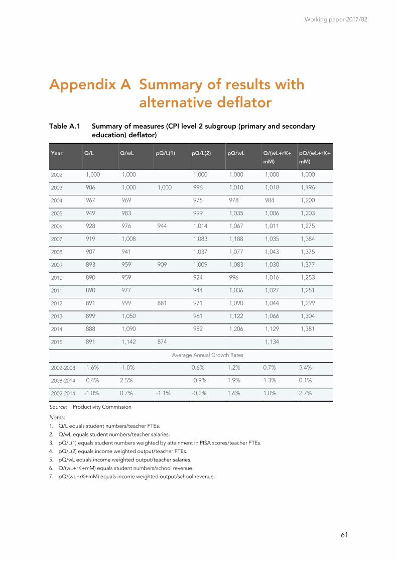
Working paper 2017/02
61
Appendix A Summary of results with alternative deflator
Table A.1 Summary of measures (CPI level 2 subgroup (primary and secondary education) deflator)
Year Q/L Q/wL pQ/L(1) pQ/L(2) pQ/wL Q/(wL+rK+
mM)
pQ/(wL+rK+
mM)
2002 1,000 1,000 1,000 1,000 1,000 1,000
2003 986 1,000 1,000 996 1,010 1,018 1,196
2004 967 969 975 978 984 1,200
2005 949 983 999 1,035 1,006 1,203
2006 928 976 944 1,014 1,067 1,011 1,275
2007 919 1,008 1,083 1,188 1,035 1,384
2008 907 941 1,037 1,077 1,043 1,375
2009 893 959 909 1,009 1,083 1,030 1,377
2010 890 959 924 996 1,016 1,253
2011 890 977 944 1,036 1,027 1,251
2012 891 999 881 971 1,090 1,044 1,299
2013 899 1,050 961 1,122 1,066 1,304
2014 888 1,090 982 1,206 1,129 1,381
2015 891 1,142 874 1,134
Average Annual Growth Rates
2002-2008 -1.6% -1.0% 0.6% 1.2% 0.7% 5.4%
2008-2014 -0.4% 2.5% -0.9% 1.9% 1.3% 0.1%
2002-2014 -1.0% 0.7% -1.1% -0.2% 1.6% 1.0% 2.7%
Source: Productivity Commission
Notes:
1. Q/L equals student numbers/teacher FTEs.
2. Q/wL equals student numbers/teacher salaries.
3. pQ/L(1) equals student numbers weighted by attainment in PISA scores/teacher FTEs.
4. pQ/L(2) equals income weighted output/teacher FTEs.
5. pQ/wL equals income weighted output/teacher salaries.
6. Q/(wL+rK+mM) equals student numbers/school revenue.
7. pQ/(wL+rK+mM) equals income weighted output/school revenue.
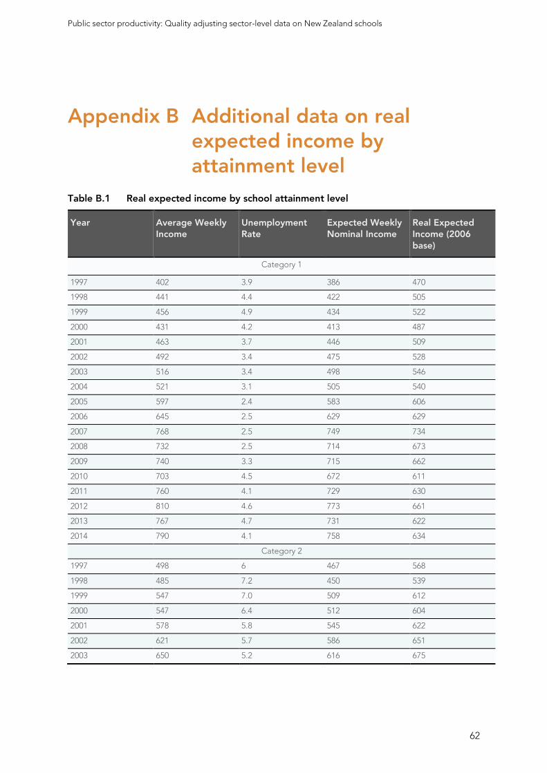
Public sector productivity: Quality adjusting sector-level data on New Zealand schools
62
Appendix B Additional data on real expected income by attainment level
Table B.1 Real expected income by school attainment level
Year Average Weekly
Income
Unemployment
Rate
Expected Weekly
Nominal Income
Real Expected
Income (2006
base)
Category 1
1997 402 3.9 386 470
1998 441 4.4 422 505
1999 456 4.9 434 522
2000 431 4.2 413 487
2001 463 3.7 446 509
2002 492 3.4 475 528
2003 516 3.4 498 546
2004 521 3.1 505 540
2005 597 2.4 583 606
2006 645 2.5 629 629
2007 768 2.5 749 734
2008 732 2.5 714 673
2009 740 3.3 715 662
2010 703 4.5 672 611
2011 760 4.1 729 630
2012 810 4.6 773 661
2013 767 4.7 731 622
2014 790 4.1 758 634
Category 2
1997 498 6 467 568
1998 485 7.2 450 539
1999 547 7.0 509 612
2000 547 6.4 512 604
2001 578 5.8 545 622
2002 621 5.7 586 651
2003 650 5.2 616 675
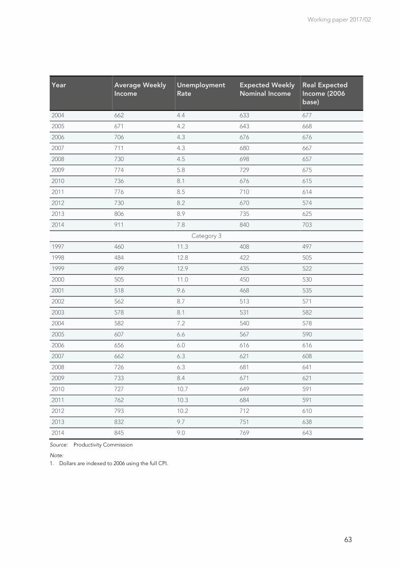
Working paper 2017/02
63
Year Average Weekly
Income
Unemployment
Rate
Expected Weekly
Nominal Income
Real Expected
Income (2006
base)
2004 662 4.4 633 677
2005 671 4.2 643 668
2006 706 4.3 676 676
2007 711 4.3 680 667
2008 730 4.5 698 657
2009 774 5.8 729 675
2010 736 8.1 676 615
2011 776 8.5 710 614
2012 730 8.2 670 574
2013 806 8.9 735 625
2014 911 7.8 840 703
Category 3
1997 460 11.3 408 497
1998 484 12.8 422 505
1999 499 12.9 435 522
2000 505 11.0 450 530
2001 518 9.6 468 535
2002 562 8.7 513 571
2003 578 8.1 531 582
2004 582 7.2 540 578
2005 607 6.6 567 590
2006 656 6.0 616 616
2007 662 6.3 621 608
2008 726 6.3 681 641
2009 733 8.4 671 621
2010 727 10.7 649 591
2011 762 10.3 684 591
2012 793 10.2 712 610
2013 832 9.7 751 638
2014 845 9.0 769 643
Source: Productivity Commission
Note:
1. Dollars are indexed to 2006 using the full CPI.
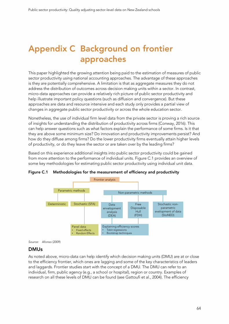
Public sector productivity: Quality adjusting sector-level data on New Zealand schools
64
Appendix C Background on frontier approaches
This paper highlighted the growing attention being paid to the estimation of measures of public
sector productivity using national accounting approaches. The advantage of these approaches
is they are potentially comprehensive. A limitation is that as aggregate measures they do not
address the distribution of outcomes across decision making units within a sector. In contrast,
micro-data approaches can provide a relatively rich picture of public sector productivity and
help illustrate important policy questions (such as diffusion and convergence). But these
approaches are data and resource intensive and each study only provides a partial view of
changes in aggregate public sector productivity or across the whole education sector.
Nonetheless, the use of individual firm level data from the private sector is proving a rich source
of insights for understanding the distribution of productivity across firms (Conway, 2016). This
can help answer questions such as what factors explain the performance of some firms. Is it that
they are above some minimum size? Do innovation and productivity improvements persist? And
how do they diffuse among firms? Do the lower productivity firms eventually attain higher levels
of productivity, or do they leave the sector or are taken over by the leading firms?
Based on this experience additional insights into public sector productivity could be gained
from more attention to the performance of individual units. Figure C.1 provides an overview of
some key methodologies for estimating public sector productivity using individual unit data.
Figure C.1 Methodologies for the measurement of efficiency and productivity
Source: Afonso (2009)
DMUs
As noted above, micro-data can help identify which decision making units (DMU) are at or close
to the efficiency frontier, which ones are lagging and some of the key characteristics of leaders
and laggards. Frontier studies start with the concept of a DMU. The DMU can refer to an
individual, firm, public agency (e.g., a school or hospital), region or country. Examples of research on all these levels of DMU can be found (see Gattoufi et al., 2004). The efficiency
Frontier analysis
Parametric methodsNon-parametric methods
Deterministic Stochastic (SFA) Data envelopment
analysis (DEA)
Free Disposable
Hull(FDH)
Panel data • Fixed effects• Random Effects
Explaining efficiency scores• Tobit regressions• Bootstrap techniques
Stochastic non-parametric
evelopment of data(StoNED)
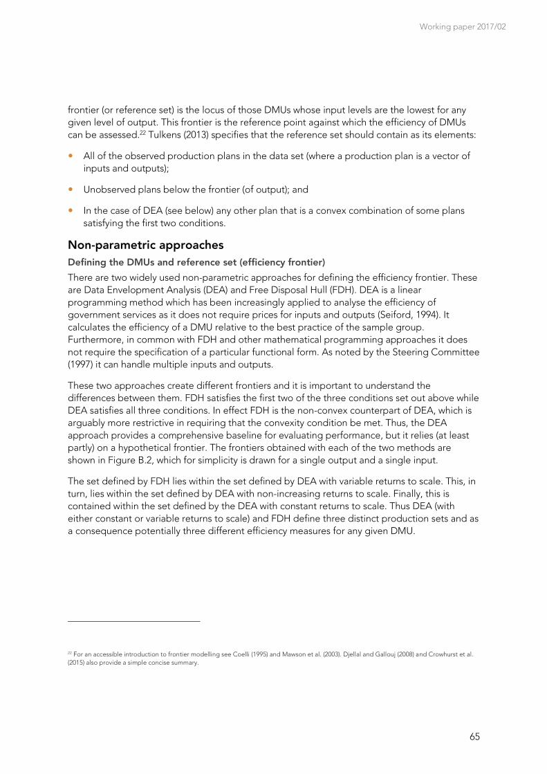
Working paper 2017/02
65
frontier (or reference set) is the locus of those DMUs whose input levels are the lowest for any
given level of output. This frontier is the reference point against which the efficiency of DMUs
can be assessed.22 Tulkens (2013) specifies that the reference set should contain as its elements:
All of the observed production plans in the data set (where a production plan is a vector of
inputs and outputs);
Unobserved plans below the frontier (of output); and
In the case of DEA (see below) any other plan that is a convex combination of some plans
satisfying the first two conditions.
Non-parametric approaches
Defining the DMUs and reference set (efficiency frontier)
There are two widely used non-parametric approaches for defining the efficiency frontier. These
are Data Envelopment Analysis (DEA) and Free Disposal Hull (FDH). DEA is a linear
programming method which has been increasingly applied to analyse the efficiency of
government services as it does not require prices for inputs and outputs (Seiford, 1994). It
calculates the efficiency of a DMU relative to the best practice of the sample group.
Furthermore, in common with FDH and other mathematical programming approaches it does
not require the specification of a particular functional form. As noted by the Steering Committee
(1997) it can handle multiple inputs and outputs.
These two approaches create different frontiers and it is important to understand the
differences between them. FDH satisfies the first two of the three conditions set out above while
DEA satisfies all three conditions. In effect FDH is the non-convex counterpart of DEA, which is
arguably more restrictive in requiring that the convexity condition be met. Thus, the DEA
approach provides a comprehensive baseline for evaluating performance, but it relies (at least
partly) on a hypothetical frontier. The frontiers obtained with each of the two methods are
shown in Figure B.2, which for simplicity is drawn for a single output and a single input.
The set defined by FDH lies within the set defined by DEA with variable returns to scale. This, in
turn, lies within the set defined by DEA with non-increasing returns to scale. Finally, this is
contained within the set defined by the DEA with constant returns to scale. Thus DEA (with
either constant or variable returns to scale) and FDH define three distinct production sets and as
a consequence potentially three different efficiency measures for any given DMU.
22 For an accessible introduction to frontier modelling see Coelli (1995) and Mawson et al. (2003). Djellal and Gallouj (2008) and Crowhurst et al.
(2015) also provide a simple concise summary.
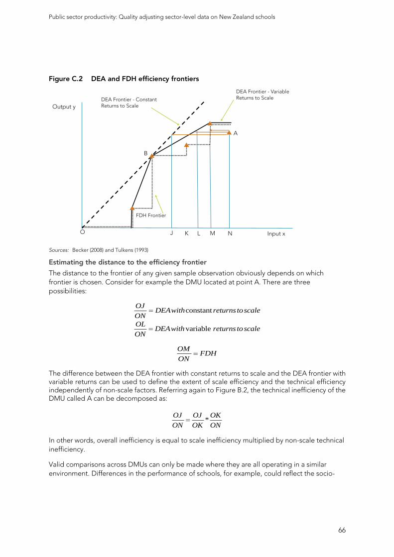
Public sector productivity: Quality adjusting sector-level data on New Zealand schools
66
Figure C.2 DEA and FDH efficiency frontiers
Sources: Becker (2008) and Tulkens (1993)
Estimating the distance to the efficiency frontier
The distance to the frontier of any given sample observation obviously depends on which
frontier is chosen. Consider for example the DMU located at point A. There are three
possibilities:
constantOJ
DEAwith returnstoscaleON
variableOL
DEAwith returns toscaleON
OMFDH
ON
The difference between the DEA frontier with constant returns to scale and the DEA frontier with variable returns can be used to define the extent of scale efficiency and the technical efficiency independently of non-scale factors. Referring again to Figure B.2, the technical inefficiency of the DMU called A can be decomposed as:
*OJ OJ OK
ON OK ON
In other words, overall inefficiency is equal to scale inefficiency multiplied by non-scale technical
inefficiency.
Valid comparisons across DMUs can only be made where they are all operating in a similar
environment. Differences in the performance of schools, for example, could reflect the socio-
Output y
Input x
DEA Frontier - Constant Returns to Scale
DEA Frontier - Variable Returns to Scale
FDH Frontier
B
A
O J K L M N
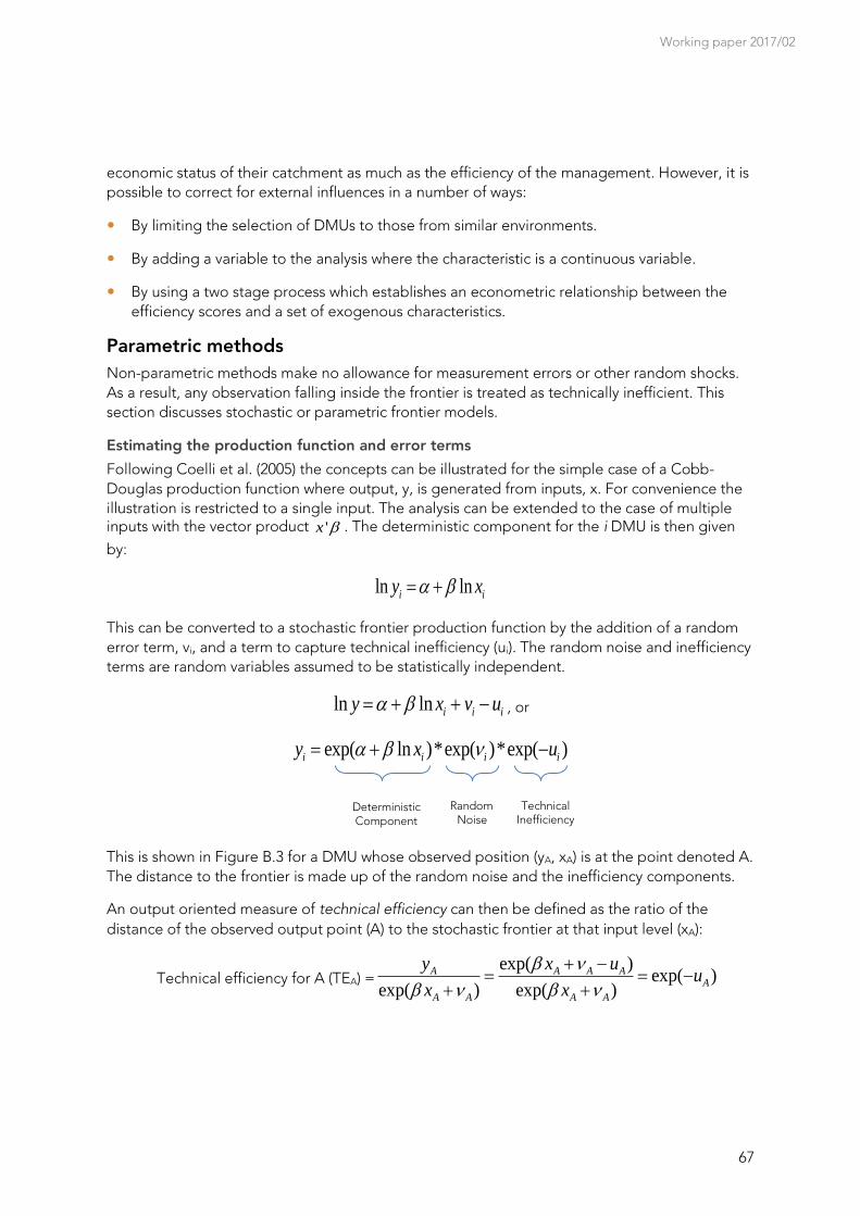
Working paper 2017/02
67
economic status of their catchment as much as the efficiency of the management. However, it is
possible to correct for external influences in a number of ways:
By limiting the selection of DMUs to those from similar environments.
By adding a variable to the analysis where the characteristic is a continuous variable.
By using a two stage process which establishes an econometric relationship between the
efficiency scores and a set of exogenous characteristics.
Parametric methods
Non-parametric methods make no allowance for measurement errors or other random shocks.
As a result, any observation falling inside the frontier is treated as technically inefficient. This
section discusses stochastic or parametric frontier models.
Estimating the production function and error terms
Following Coelli et al. (2005) the concepts can be illustrated for the simple case of a Cobb-
Douglas production function where output, y, is generated from inputs, x. For convenience the
illustration is restricted to a single input. The analysis can be extended to the case of multiple inputs with the vector product 'x . The deterministic component for the i DMU is then given
by:
ln lni iy x
This can be converted to a stochastic frontier production function by the addition of a random
error term, vi, and a term to capture technical inefficiency (ui). The random noise and inefficiency
terms are random variables assumed to be statistically independent.
ln ln i i iy x v u , or
exp( ln )*exp( )*exp( )i i i iy x u
This is shown in Figure B.3 for a DMU whose observed position (yA, xA) is at the point denoted A.
The distance to the frontier is made up of the random noise and the inefficiency components.
An output oriented measure of technical efficiency can then be defined as the ratio of the
distance of the observed output point (A) to the stochastic frontier at that input level (xA):
Technical efficiency for A (TEA) =exp( )
exp( )exp( ) exp( )
A A A AA
A A A A
y x uu
x x
Deterministic Component
Random Noise
Technical Inefficiency
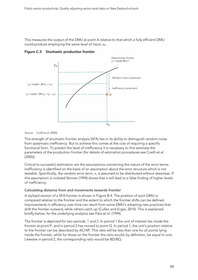
Public sector productivity: Quality adjusting sector-level data on New Zealand schools
68
This measures the output of the DMU at point A relative to that which a fully efficient DMU
could produce employing the same level of input, xA.
Figure C.3 Stochastic production frontier
Source: Coelli et al. (2005)
The strength of stochastic frontier analysis (SFA) lies in its ability to distinguish random noise
from systematic inefficiency. But to achieve this comes at the cost of requiring a specific
functional form. To predict the level of inefficiency it is necessary to first estimate the parameters of the production frontier (for details of estimation procedures see Coelli et al.
(2005)).
Critical to successful estimation are the assumptions concerning the nature of the error terms.
Inefficiency is identified on the basis of an assumption about the error structure which is not testable. Specifically, the random error term, v, is assumed to be distributed without skewness. If
this assumption is violated Skinner (1994) shows that it will lead to a false finding of higher levels
of inefficiency.
Calculating distance from and movements towards frontier
A stylised version of a SFA frontier is shown in Figure B.4. The position of each DMU is
compared relative to the frontier and the extent to which the frontier shifts can be defined.
Improvements in efficiency over time can result from some DMU’s adopting new practices that
shift the frontier outward, while others catch up (Cullen and Ergas, 2014). This is explained briefly below; for the underlying analytics see Färe et al. (1994).
The frontier is depicted for two periods, 1 and 2. In period 1 the unit of interest lies inside the
frontier at point P, and in period 2 has moved to point Q. In period 1, the unit’s position relative
to the frontier can be described by AC/AP. This ratio will be less than one for all points lying
inside the frontier, while for those on the frontier the ratio would, by definition, be equal to one.
Likewise in period 2, the corresponding ratio would be BD/BQ.
Deterministic frontieryi = exp(α+βlnxi )
A
Random noise component
Inefficiency component
xA
yA
yA= exp(α + βlnxA + νA )
yA= exp(α + βlnxA + νA - u A)
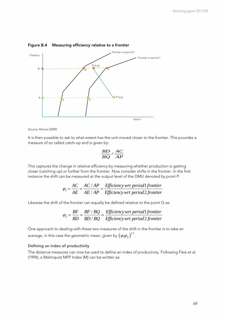
Working paper 2017/02
69
Figure B.4 Measuring efficiency relative to a frontier
Source: Afonso (2009)
It is then possible to ask to what extent has the unit moved closer to the frontier. This provides a
measure of so called catch-up and is given by:
/BD AC
BQ AP
This captures the change in relative efficiency by measuring whether production is getting
closer (catching up) or further from the frontier. Now consider shifts in the frontier. In the first
instance the shift can be measured at the output level of the DMU denoted by point P:
1
/ 1
/ 2
AC AC AP Efficiency wrt period frontier
AE AE AP Efficiency wrt period frontier
Likewise the shift of the frontier can equally be defined relative to the point Q as:
2
/ 1
/ 2
BF BF BQ Efficiencywrt period frontier
BD BD BQ Efficiencywrt period frontier
One approach to dealing with these two measures of the shift in the frontier is to take an
average, in this case the geometric mean, given by 1/2
1 2 .
Defining an index of productivity
The distance measures can now be used to define an index of productivity. Following Färe et al.
(1994), a Malmquist MFP Index (M) can be written as:
Public sector productivity: Quality adjusting sector-level data on New Zealand schools
70
1/2BD AP AC BF
MBQ AC AE BD
The term in square brackets is the geometric mean of the shift in technology between the two
periods, i.e., the extent of technical change. The ratio outside the square brackets is the input
oriented measure of technical efficiency or catching up. In summary, the MFP index can be
decomposed into an element of technical efficiency which captures the diffusion of technology
and an element measuring technological change or innovation. In its simplest terms the
Malmquist measure for productivity change can be viewed as:
( )*( )M Diffusion Innovation
How does this result relate to that of growth accounting? Färe et al. (1994) illustrate the case for
a Cobb-Douglas production function of the standard form:
i
t t it
i
y A x
and show that M is simply the ratio of the Solow efficiency parameters (At) or:
1t
t
AM
A
This result, however, depends critically on the assumption that the actual output levels lie on the
frontier, so the growth accounting measure of multi factor productivity is simply capturing the
technological shift. When observed outputs lie on the frontier the distance functions are by
definition equal to one. As a consequence the diffusion term is unity and M measures just the
innovation or technological change effect. In other words, a standard growth accounting
measure of MFP derived from a Cobb-Douglas production function will be biased if there is any
inefficiency such that some observed outputs fall inside the frontier. Indeed, Coelli (2002)
stresses that the Malmquist MFP index will only properly measure productivity changes if the
underlying technology used to generate the input distance functions for M display constant
returns to scale.
Conclusion
Observations of the inputs and outputs of DMUs can be used to define a frontier. This efficiency
frontier (or reference set) is the locus of those DMUs whose input levels are the lowest for any
given level of output. This frontier is the reference point against which the efficiency of a DMU
can be assessed. Two useful techniques for defining a frontier are data envelopment analysis
(DEA) and stochastic frontier analysis (SFA). Considerations when choosing between them
include:
Cases with less heterogeneous samples are more suited to DEA. SFA is more suitable for
more heterogeneous samples. DEA is more sensitive to heterogeneity in the sample
(influenced by outliers) and will tend to give lower average efficiency scores (although not
consistently so). The regression approach of SFA means outliers are given less weight.
Working paper 2017/02
71
Cases where output supplied is subject to variable and/or unpredictable client demand are
less suited to DEA. Unpredictability of client demand can introduce a source of variance in
outputs and make the input-output relationship for a DEA stochastic. SFA is better suited to
coping with unpredictable demand.
Both methods can deal with cases where operating environments are influenced by
exogenous variables. Where these variables could be an important consideration a DEA
approach of restricting the comparison set (to DMUs that have similar or less favourable
operating environments) is likely to be less suitable. Other DEA approaches or an SFA
approach based on regression analysis would be better.
SFA requires the parameters of the production function and the random error term to be
estimated. DEA is more suitable for cases where these parameters cannot be feasibly
estimated, such as where there are a limited number of observations available for robust
regression analysis.