PUBLICATIONS - Penn State Meteo Computing … · Second, GCM projections have large uncertainties (depending upon the region) mainly due to parameter-ization of cloud physics, uncertainty

RESEARCH ARTICLE10.1002/2013WR014988

A vulnerability driven approach to identify adverse climate andland use change combinations for critical hydrologic indicatorthresholds: Application to a watershed in Pennsylvania, USAR. Singh1, T. Wagener2, R. Crane3, M. E. Mann4, and L. Ning5

1Earth and Environmental Systems Institute, Pennsylvania State University, University Park, Pennsylvania, USA,2Department of Civil Engineering, University of Bristol, Bristol, UK, 3Department of Geography, Pennsylvania StateUniversity, University Park, Pennsylvania, USA, 4Department of Meteorology, Pennsylvania State University, UniversityPark, Pennsylvania, USA, 5Northeast Climate Science Center, Department of Geosciences, University ofMassachusetts-Amherst, Amherst, Massachusetts, USA

Abstract Large uncertainties in streamflow projections derived from downscaled climate projections ofprecipitation and temperature can render such simulations of limited value for decision making in the con-text of water resources management. New approaches are being sought to provide decision makers withrobust information in the face of such large uncertainties. We present an alternative approach that startswith the stakeholder’s definition of vulnerable ranges for relevant hydrologic indicators. Then the modeledsystem is analyzed to assess under what conditions these thresholds are exceeded. The space of possibleclimates and land use combinations for a watershed is explored to isolate subspaces that lead to vulnerabil-ity, while considering model parameter uncertainty in the analysis. We implement this concept using classi-fication and regression trees (CART) that separate the input space of climate and land use change intothose combinations that lead to vulnerability and those that do not. We test our method in a Pennsylvaniawatershed for nine ecological and water resources related streamflow indicators for which an increase intemperature between 3�C and 6�C and change in precipitation between 217% and 19% is projected. Ourapproach provides several new insights, for example, we show that even small decreases in precipitation(�5%) combined with temperature increases greater than 2.5�C can push the mean annual runoff into aslightly vulnerable regime. Using this impact and stakeholder driven strategy, we explore the decision-relevant space more fully and provide information to the decision maker even if climate change projectionsare ambiguous.

1. Introduction

Freshwater availability is essential for maintaining both the ecological and economic health of a region. Weneed reliable projections of future streamflow under changing environmental conditions to guide long-term water resources management and planning [Milly et al., 2002, 2008; Wagener et al., 2010]. The informa-tion about future streamflow is required at the scale of regional planning [Barron, 2009]. However,obtaining this information can be difficult due to large uncertainties in regional estimates of climate changeprojections [Hall, 2007; Beven, 2011; Collins et al., 2012].

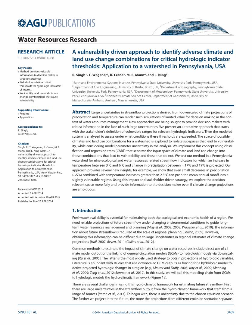
Common methods to estimate the impact of climate change on water resources include direct use of cli-mate model output or the linking of general circulation models (GCMs) to hydrologic models via downscal-ing [Xu et al., 2005]. The latter is the most widely used strategy to obtain projections of hydrologic variables.Literature is abundant with studies that use downscaled GCM outputs as forcing for a hydrologic model toderive projected hydrologic changes in a region [e.g., Maurer and Duffy, 2005; Kay et al., 2009; Manninget al., 2009; Teng et al., 2012; Bennett et al., 2012]. In this study, we will call this modeling chain from GCMsto hydrologic models the hydro-climatic framework (Figure 1a).

There are several challenges in using this hydro-climatic framework for estimating future streamflow. First,there are large uncertainties in the streamflow output from the hydro-climatic framework that stem from arange of sources [Paton et al., 2013]. To begin with, there is uncertainty due to the chosen emission scenario.The further we project into the future, the more the projections from different emission scenarios separate.

Key Points:� Method provides valuable

information to decision maker inlarge uncertainties� Stakeholders define critical

thresholds for hydrologic indicatorsof interest� We identify land use and climate

change combinations that causevulnerability

Supporting Information:� Readme� Appendices

Correspondence to:R. Singh,[email protected]

Citation:Singh, R., T. Wagener, R. Crane, M. E.Mann, and L. Ning (2014), Avulnerability driven approach toidentify adverse climate and land usechange combinations for criticalhydrologic indicator thresholds:Application to a watershed inPennsylvania, USA, Water Resour. Res.,50, 3409–3427, doi:10.1002/2013WR014988.

Received 4 NOV 2013

Accepted 5 APR 2014

Accepted article online 10 APR 2014

Published online 25 APR 2014

SINGH ET AL. VC 2014. American Geophysical Union. All Rights Reserved. 3409

Water Resources Research

PUBLICATIONS

http://dx.doi.org/10.1002/2013WR014988

http://onlinelibrary.wiley.com/journal/10.1002/(ISSN)1944-7973/

http://publications.agu.org/

Second, GCM projections have large uncertainties (depending upon the region) mainly due to parameter-ization of cloud physics, uncertainty in climate sensitivity, etc. The overlap in the underlying physics in thesemodels limits our ability to construct an ensemble of climate models that can reasonably estimate the prob-ability distribution of climate projections, since they do not represent independent samples [Stephensonet al., 2012; Knutti et al., 2013]. There are also significant uncertainties in the hydrologic model, includingmodel structural uncertainty and a dependence of the model parameters on the climate in the calibrationperiod [Merz et al., 2010; Singh et al., 2011, 2013]. A priori parameters can be used instead, but generallyexhibit large uncertainties if these are estimated [Kapangaziwiri et al., 2012]. Hence the traditional forwardpropagation approach that integrates uncertainty from different sources may lead to biased or overconfi-dent hydrologic projections that might be ineffective in aiding decision makers [Hall, 2007; Beven, 2011].

So while we generally assume that significant amount of uncertainties are present, we do not know theactual amount and we often lack the ability to attribute the total estimated uncertainty to its sources (e.g.,choice of GCM, downscaling, GCM parameters, etc.). The contribution of different sources of uncertainty tothe total uncertainty in streamflow projections depends on the study region, the hydrologic indicator con-sidered, the hydrologic model used, etc. [Chen et al., 2011; Dobler et al., 2012; Teng et al., 2012; Bosshardet al., 2013]. For example, Teng et al. [2012] find that streamflow projections are more uncertain for drierregions within their study area in southeastern Australia. They also find that uncertainties in projections oflow flow characteristics are higher for regions that are likely to experience large declines in future rainfall.Chen et al. [2011] also show that the relative contribution of uncertainty from different sources varies withthe hydrologic metric being evaluated. Dobler et al. [2012] show that even though GCM uncertainties domi-nate hydrologic projections for most of the year, the uncertainty from hydrologic model parameters isgreater than uncertainty from GCMs during some winter months. These recent findings also challenge theconclusions from earlier studies that the uncertainty arising from GCMs or downscaling methods often over-shadows those originating from the choice of hydrologic model structure or hydrologic model parameters[Wilby and Harris, 2006; Kay et al., 2009; Prudhomme and Davies, 2009a, 2009b].

While traditional forward propagation approaches (Figure 1a) may be used to gain understanding of possi-ble changes in streamflow, decision makers do not always find this information helpful given that they canoften include projections that suggest both positive and negative changes in streamflow (mainly due toprecipitation). Recent studies have proposed alternative bottom-up or vulnerability-based approaches fordealing with problems such as water management decisions under large projection uncertainties [Lempertet al., 2008; Wilby and Dessai, 2010; Brown et al., 2011; Weaver et al., 2013]. In essence, these alternative para-digms invert the problem by following a ‘‘bottom-up’’ approach as shown in Figure 1b. Here stakeholdersdefine vulnerability ranges for a particular decision variable, e.g., a specific hydrologic indicator, from theoutset. Then all combinations of climatic input and model parameters that cause the variable of interest totransition into vulnerable regimes are identified through a modeling framework. Finally, the available

d y s

nd

us

n u

Emission scenarios (future CO2 concentration) Determine plausibility of

vulnerability

.b.a

General circulation models

Downscalingal fo

rwar

tion

p an

alys

i

Hydrologic model

Indicators of hydrologic

Trad

itio

prop

aga Identify regions in

framework space that lead to vulnerability

Bot

tom

response

Determine if these ranges fall in the vulnerable region

Determine vulnerability ranges for the hydrologic indicator

Figure 1. (a) The hydro-climatic framework showing the traditional forward propagation approach used to derive future changes in hydro-logic variables of interest and (b) the bottom-up approach used in this study, which starts by defining different (slightly vulnerable/vulner-able/nonvulnerable, etc.) classes for a hydrologic indicator of interest and then identifying the regions in the input space that lead to eachclass.

Water Resources Research 10.1002/2013WR014988


information on future climate is integrated to assess the plausibility of the hydrologic indicator to transitioninto a vulnerable regime in the future.

These bottom-up approaches are sometimes also termed decision scaling or context-first approaches. Theycan be used in a wide variety of problems and have proved very useful for decision making when projec-tions of the future are highly uncertain [Moody and Brown, 2013; Kunreuther et al., 2013]. Lempert et al.[2008] describe two possible methods to identify vulnerable regions in the input space—patient rule induc-tion method (PRIM) and classification and regression trees (CART). Neither of these methods is found to besignificantly superior to the other in Lempert et al. [2008]. However, PRIM is generally employed when theoutput space is partitioned in two possibilities—vulnerable or nonvulnerable. Other example applicationsof these alternative approaches include risk-based decision making to characterize contaminant plumes byBoso et al. [2013], and the use of decision tree models for estimating the value of information provided by agroundwater quality monitoring network by Khader et al. [2013].

In this study, we present a method based on this bottom-up paradigm that provides decision makers withinformation about adverse thresholds in climate and land use change that may cause a hydrologic indicatorto transition to vulnerable regimes. These thresholds can directly be used to inform policy decisions even ifuncertainties in future climate projections are large. For example, if an indicator quickly transitions into vul-nerable regimes (small changes in climate or land use causing vulnerability—low thresholds), it providesthe decision maker with the foresight that a very robust policy or drastic actions will be needed to avoidpotentially large damages. In this way, the information about thresholds in climate or land use obtainedcan be combined with the available information on projected climate change (with small or large range ofuncertainties) to provide the decision maker with better insights into the nature of the hydrologic indicator,its dominant controls, possible tipping points, feasibility of crossing those tipping points, etc.

The objective of our study is to implement and test a classification tree method centered on a vulnerability-based approach for change assessment. We test our approach in the Lower Juniata watershed in Pennsylva-nia located in the northeastern USA for nine different hydrologic (streamflow) indicators. We derive classifi-cation trees for these indicators using a large range of possible climates, land uses, and hydrologic modelparameters. The large range of climates is generated by applying the delta change method to precipitationand temperature time series to the historical period of 1948–1958. A vegetation parameter in the hydro-logic model approximates the land use and uncertainty in the ranges for other hydrologic model parame-ters is based on their a priori values derived from the watershed physical characteristics.

Using these classification trees, we demonstrate how our proposed method provides additional informationto a decision maker as compared to the standard approach by generating estimates of critical thresholds inclimate as well as an understanding of relative importance of climate and land use change within thehydrologic modeling framework. For example, the available downscaled projections of climate from ninegeneral circulation models (GCMs) for the baseline (1990–2000) and end of century (2090–2100) time peri-ods are used to navigate the classification tree to arrive at the future values of the indicators (e.g., meanannual runoff) and assess the impact of changing climate on the hydrologic indicator. We then comparethe projections from the classification tree-based approach to those from the standard approach by drivinga historically calibrated hydrologic model using future projections of downscaled climate.

2. Methodology, Model, and Data

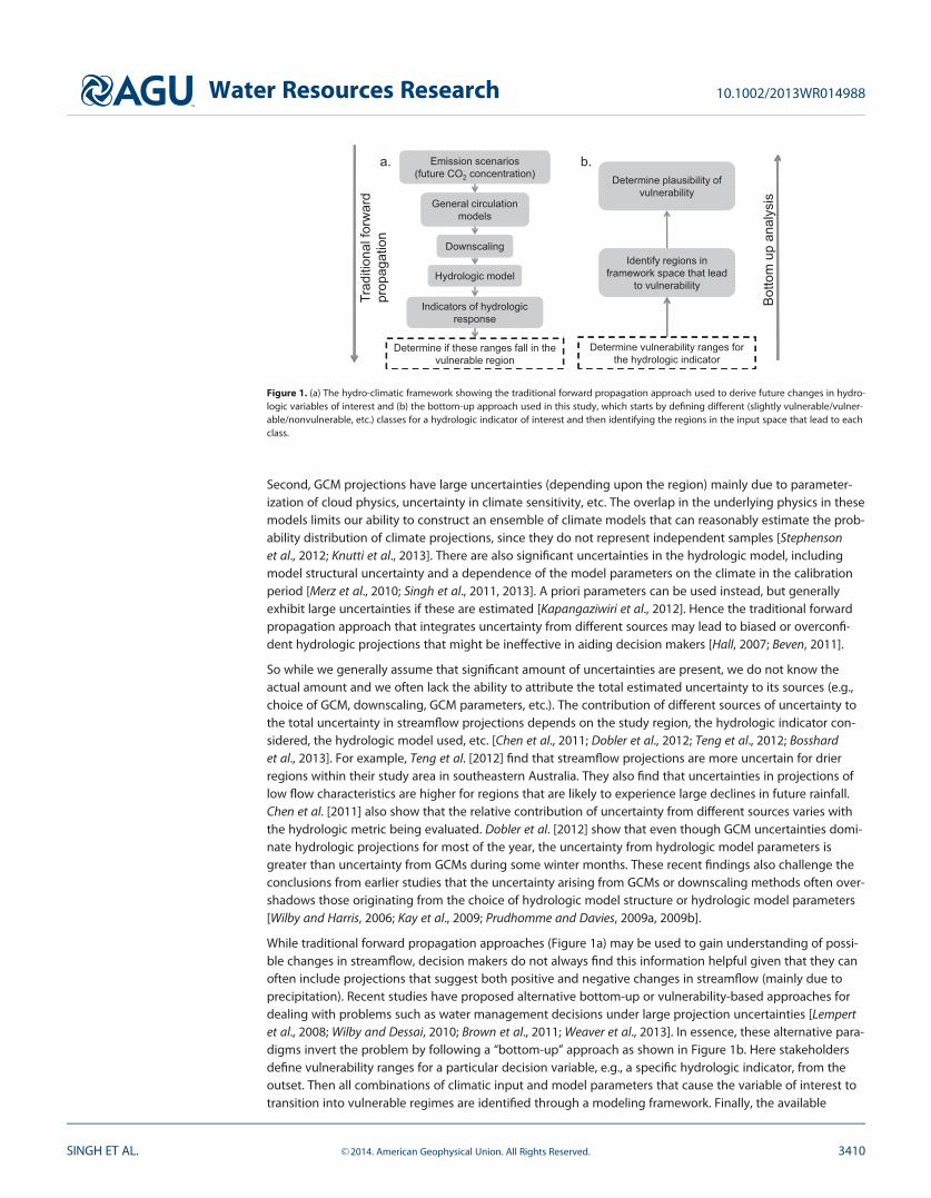
2.1. A Classification Tree-Based Strategy for Identifying Critical Climate and Land Use ChangeCombinationsThe main goal of our study is to establish the relationship between different possible climate and land usechanges in our study watershed and resulting streamflow indicator values (Figure 2). To achieve this goal,we invert the problem through exploratory modeling. We start by defining a feasible space of climate andland use changes. Land use is represented as a parameter representing the fraction of deep-rooted vegeta-tion in the watershed—assuming that this is main aspect of vegetation that matters for the hydrologic indi-cators studied here. Other processes and land use characteristics can be easily included. Different feasibleclimates are generated using the delta change method in which only the mean of the climate variables(precipitation and temperature) is changed keeping the higher moments fixed [Nash and Gleick, 1991; Joneset al., 2006]. Following this definition of the feasible input space, we establish different classes for the



hydrologic indicator of interest.Here the stakeholder would nor-mally be asked to provide theirdefinition of vulnerable ranges ofstreamflow indicators. This couldfor example be an ecologist whodefines critical values for a partic-ular aquatic species, or a waterresources manager who has tofulfill multiple competingdemands throughout the year.

In our study, we establish the fol-lowing grouping to demonstratethe methodology: if the value ofthe selected indicator is withinhistorical variability, it falls inClass 1, if it is only slightly abovehistorically observed values, it isassigned Class 2, and extremeincreases are grouped in Class 6.We develop similar classes forvalues that are below the

observed historical variability. Each resultant value of the hydrologic indicator obtained from a particularcombination of climate and land use can then be assigned a class based on these class definitions. Eventhough we start with a possible classification of hydrologic indicator space to demonstrate the method,stakeholders can adjust this approach by defining their own vulnerability classes and identify how climateor land use change will impact the indicators that most interest them. This will allow them to have anunderstanding of not just the specific projections of streamflow based on climate model outputs but thegeneral behavior of their indicator. Using the mapping from input climate and land use space to outputindicator space, they can decide how robust the policy for dealing with future changes should be.

Using N climates and P parameter combinations, we derive N 3 P values of hydrologic indicators of interestby driving the hydrologic model with these combinations and assign them to their specific class. Next, weuse the classification and regression tree (CART) to relate the climate and land use changes to the differentclasses of the streamflow indicator. CART is a binary recursive partitioning algorithm that divides the inputspace of multiple variables into subspaces, with each subspace related to a particular class of output vari-able [Breiman et al., 1984]. At each stage, the tree partitions the space based on maximum gain in informa-tion. Thus, through CART analysis, we can assess the critical changes in land use and climate required topush the streamflow indicators into different regimes (represented by the indicator classes). Once we obtainthe information regarding the critical combinations in climate and land use, we can include the availabledownscaled climate data into the analysis. Using the future projections of climate change derived fromdownscaled GCMs, we can assess the plausibility of the hydrologic indicator to transition into a vulnerableregime. Similarly, we could assess specific land use change scenarios for the study region.

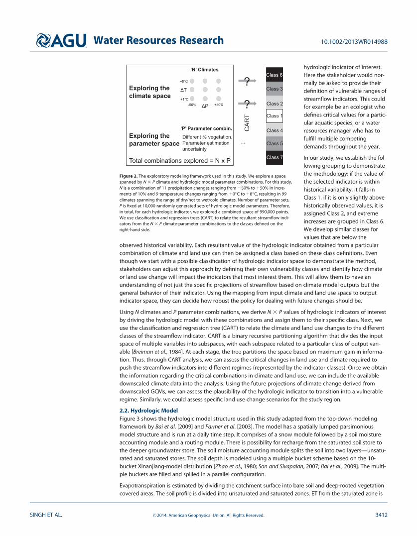
2.2. Hydrologic ModelFigure 3 shows the hydrologic model structure used in this study adapted from the top-down modelingframework by Bai et al. [2009] and Farmer et al. [2003]. The model has a spatially lumped parsimoniousmodel structure and is run at a daily time step. It comprises of a snow module followed by a soil moistureaccounting module and a routing module. There is possibility for recharge from the saturated soil store tothe deeper groundwater store. The soil moisture accounting module splits the soil into two layers—unsatu-rated and saturated stores. The soil depth is modeled using a multiple bucket scheme based on the 10-bucket Xinanjiang-model distribution [Zhao et al., 1980; Son and Sivapalan, 2007; Bai et al., 2009]. The multi-ple buckets are filled and spilled in a parallel configuration.

Evapotranspiration is estimated by dividing the catchment surface into bare soil and deep-rooted vegetationcovered areas. The soil profile is divided into unsaturated and saturated zones. ET from the saturated zone is

‘N’ Climates

P

Exploring the climate space

Exploring the parameter space

T

‘P’ Parameter combin. Different % vegetation, Parameter estimation uncertainty

Total combinations explored = N x P

?

...

?

+8°C

+1°C -50% +50%

CA

RT

Class 5

Class 6

Class 2

Class 1

Class 3

Class 7

Class 4

Figure 2. The exploratory modeling framework used in this study. We explore a spacespanned by N 3 P climate and hydrologic model parameter combinations. For this study,N is a combination of 11 precipitation changes ranging from 250% to 150% in incre-ments of 10% and 9 temperature changes ranging from 10�C to 18�C, resulting in 99climates spanning the range of dry/hot to wet/cold climates. Number of parameter sets,P is fixed at 10,000 randomly generated sets of hydrologic model parameters. Therefore,in total, for each hydrologic indicator, we explored a combined space of 990,000 points.We use classification and regression trees (CART) to relate the resultant streamflow indi-cators from the N 3 P climate-parameter combinations to the classes defined on theright-hand side.



proportional to potential evapora-tion and the soil moisture con-tent. The saturated zone ET ismodeled similarly for both baresoil and vegetation covered frac-tions. The main difference in ETarises within the unsaturated soilstore. In the unsaturated zone, thefraction of the watershed coveredby bare soils evaporates at a ratethat is proportional to the soilwater content and to the poten-tial evaporation. While in the caseof vegetation-covered soils, tran-spiration from the unsaturatedstores is controlled by fieldcapacity parameter. If the soilmoisture content exceeds fieldcapacity, transpiration occurs at

potential rate. The basic formulation is adapted from Bai et al. [2009], with modifications for including phenol-ogy and leaf area index from Sawicz [2013]. Equations are included in supporting information (Appendix A).

The growing behavior of vegetation, efficiency of water extraction from the soil, and variable canopy inter-ception are included in the model to represent phenology in three ways. Above 10�C, water extraction byvegetation is considered unimpeded and is set at its maximum capacity. Below 25�C, water extraction effi-ciency is considered to have stopped so there is no evapotranspiration. Between these two ranges, a linearrelationship between extraction efficiency and temperature is assumed. The canopy interception is mod-eled as maximum canopy interception during summer months and a minimum during winter months. Asinusoidal function is used to describe the canopy interception for periods between summer and winter.Details of model equations are provided in supporting information (Appendix A) and Table 2 lists the feasi-ble range of parameters based on literature review.

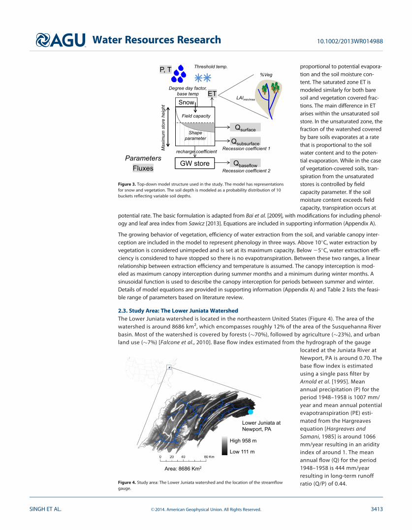
2.3. Study Area: The Lower Juniata WatershedThe Lower Juniata watershed is located in the northeastern United States (Figure 4). The area of thewatershed is around 8686 km2, which encompasses roughly 12% of the area of the Susquehanna Riverbasin. Most of the watershed is covered by forests (�70%), followed by agriculture (�23%), and urbanland use (�7%) [Falcone et al., 2010]. Base flow index estimated from the hydrograph of the gauge

located at the Juniata River atNewport, PA is around 0.70. Thebase flow index is estimatedusing a single pass filter byArnold et al. [1995]. Meanannual precipitation (P) for theperiod 1948–1958 is 1007 mm/year and mean annual potentialevapotranspiration (PE) esti-mated from the Hargreavesequation [Hargreaves andSamani, 1985] is around 1066mm/year resulting in an aridityindex of around 1. The meanannual flow (Q) for the period1948–1958 is 444 mm/yearresulting in long-term runoffratio (Q/P) of 0.44.

hm

h

parameterm parameter

FluxesFluxes

Threshold temp.P, T%Veg

SnowET

t

Degree day factor, base temp

LAImin/max

um s

tore

hei

g

Shape

Field capacity

Qsurface

GW storeM

axi

Qbaseflow

Recession coefficient 1recharge coefficientParameters

Qsubsurface

Recession coefficient 2

Figure 3. Top-down model structure used in the study. The model has representationsfor snow and vegetation. The soil depth is modeled as a probability distribution of 10buckets reflecting variable soil depths.

High 958 m

Low 111 m

Area: 8686 Km2

Lower Juniata at Newport, PA

Figure 4. Study area: The Lower Juniata watershed and the location of the streamflowgauge.



2.4. DataThe historical streamflow, temperature, and precipitation data are obtained from the MOPEX data set [Duanet al., 2006]. The downscaled climate data used in the study are derived using the probabilistic downscalingmethod by Ning et al. [2012a, 2012b]. Table 3 lists the number of global climate models (GCMs) used forthis analysis. We also use the data from Falcone database [Falcone et al., 2010] for obtaining watershedproperties such as land use, soil types, etc. to derive a priori ranges of hydrologic model parameters.

2.5. Classification and Regression TreesClassification and regression tree (CART) is a recursive partitioning algorithms used to classify the spacedefined by the input variables (here hydrologic model parameters and climate) based on the output vari-able (here categorized hydrologic indicators) [Breiman et al., 1984]. In this study, we apply CART analysisusing the statistical CART package of R called ‘‘rpart’’ [Therneau and Atkinson, 2010]. This method automati-cally provides a pruned tree after a tenfold cross validation and also provides estimates for the misclassifica-tion error rates and cross-validation error rates for the classification trees developed.

The resulting tree consists of a series of nodes, where each node is a logical expression based on the valuesof a hydrologic model parameter or a climate variable in the input space. If the expression is true, the leftbranch is followed; otherwise, the right branch is followed. In this way, one can follow different combina-tions of expressions (representing multidimensional subspaces of the input variables) to arrive at a terminalleaf, which represents the output variable class with the highest probability. Since the classification is imper-fect, the CART analysis also provides information on the probabilities of different output classes at each ter-minal leaf node. The histograms of class distributions at each terminal leaf node visualize theseprobabilities, thereby providing an assessment of the uncertainty associated with the classification.

3. Results

3.1. Obtaining A Priori Ranges for Hydrologic Model ParametersWe include parametric uncertainty in this analysis by obtaining a priori parameter ranges largely based onphysical watershed characteristics. This is achieved in two ways—relating the different components of thehydrologic model with observed physical characteristics of the watershed from the Falcone database andrecession curve analysis of the historical streamflow data. Using this approach, a priori ranges are obtainedfor 7 out of 12 parameters. For the remaining parameters, feasible ranges are obtained from literature[Farmer et al., 2003; Van Werkhoven et al., 2008; Bai et al., 2009; Kollat et al., 2013]. The a priori ranges areestimated for two recession parameters, two soil parameters and three vegetation parameters.

We derive a priori ranges for two parameters related to the soil module—soil depth and field capacity. Soildepth is obtained based on the available depth to bedrock estimates, and porosity estimates of sand, silt,and clay (all three are present in the watershed in significant amounts—50% silt, 30% sand, and 20% clay).Field capacity parameter range is estimated as the range of the field capacity parameter across sand, silt,and clay using the information on watershed average available water capacity, porosity, and permanentwilting point ranges for sand, silt, and clay. Vegetation parameter is estimated from land use informationabout the watershed [Falcone et al., 2010]. The percentage forest cover in the watershed is around 70%, sothe range of fraction of deep-rooted vegetation in the watershed is fixed between 0.6 and 0.8. Leaf areaindex values are fixed between 0 and 6, since most the forests are deciduous in nature. Supporting informa-tion Tables B1–B3 lists these calculations in details.

Two recession parameters are present in the model—recession coefficient 1 (Ass) for subsurface flow fromthe saturated store and recession coefficient 2 (Abf) for base flow from the groundwater reservoir. These areobtained from analyzing the recession behavior of the available streamflow time series. Since the modeldoes not route the surface flow, recession analysis is carried out only on base flow component of the totalstreamflow, which is derived from the base flow filter [Arnold et al., 1995]. Two slopes are estimated foreach year across a 10 year time period. Recession coefficient 1, which represents the recession from satu-rated store, is estimated as the average slope across the fast recession limbs (6–14 days). Recession coeffi-cient 2, which represents the recession from the groundwater reservoir, is estimated by constructing amaster recession curve for the recession after removing the faster recession limbs (40–83 days). Figures B1



and B2 show the estimation procedure of routing parameters as derived from the streamflow hydrographsand Table 2 lists the ranges.

3.2. Climate ScenariosThe delta change method described in section 2.1 is used to generate climate change scenarios. The histori-cal period of 1948–1958 is used as the base period and changes in temperature and precipitation areapplied on the climate time series for this period. The ranges for precipitation change explored are 250%to 150% in steps of 10%. The ranges for temperature change are 0–8�C in steps of 1�C. Therefore, the totalnumber of climate combinations explored is 99. The adjustments to the climate data were made at dailytime steps with the precipitation values multiplied by a suitable fraction between 0.5 and 1.5 and the tem-perature values increased by 0–8�C. To provide an estimate of how wide these ranges are—the IPCC 4thassessment report [Christensen et al., 2007] suggests changes in precipitation between 23% and 15% andtemperature increase between 2.3�C and 5.6�C from 1980–1999 to 2080–2099 for Eastern United Statesunder the A1B emission scenario. It is important to note here that we use two different climate data in thestudy—the climates generated from the delta change method are used to explore the feasible climatespace, whereas the downscaled climate data by Ning et al. [2012a, 2012b] are used once the (synthetic) cli-mate and land use space has been related to the hydrologic indicator. The synthetic climate data are usedto explore the climate space and build the classification trees. The downscaled climate data are used toassess the plausibility of the watershed to transition into a vulnerable regime in section 3.8 once the tree isderived.

3.3. Defining Classes for Streamflow IndicatorsIn this study, we assume that we want to analyze the major controls on indicators representing aspects ofstreamflow relevant for ecology as well as water availability for human abstractions such as power genera-tion. Magnitude-related indicators such as mean annual runoff would determine average water availability.Seasonal variability of water availability will be represented by indicators related to flow in months of high/low flows. Olden and Poff [2003] describe several indicators that are ecologically relevant as well as repre-sent water availability. Based on the insights provided by them, we include four categories of indicators inour analysis (Table 1).

1. Magnitude-related indicators include mean annual runoff, minimum April flow, and maximum Augustflow. As shown in Figure B3, August is a low-flow month for this watershed, and April is a high-flow month.Therefore, flows for both months are included in the analysis.

2. Frequency-related indicators include low flow pulse count and flood frequency. These are important toassess the recurrence of low/high-flow conditions in the watershed, which will be critical for in stream floraand fauna.

3. Duration-related indicators include low flow pulse duration and high flow pulse duration. Low flow pulseduration is particularly important since it assesses the number of days low flows will sustain in the water-shed and is very important to assess water availability for power production during summer months.

Table 1. Definition of Hydrologic Indicators Analyzed in the Study Based on Olden and Poff [2003]

Hydrologic Indicator Category Definition Units

Mean annual runoff Magnitude Mean annual flow (normalized by catchment area) mm/yearMinimum April flow Magnitude—high Mean minimum monthly flow for April across time period of study mm/dayMaximum August flow Magnitude—low Mean maximum monthly flow for August across time period of study mm/dayLow flow pulse count Frequency—low Number of annual occurrences during which the magnitude of flow remains below a

lower threshold. Hydrologic pulses are defined as those periods within a year inwhich the flow drops below 25th percentile of all daily values for the time period

Flood frequency Frequency—high Same as above where high pulse is defined as three times the median daily flowLow flow pulse duration Duration—low Mean duration of low flow pulses defined above daysHigh flow pulse duration Duration—high Mean duration of high flow pulses with high flow cutoff at 75th percentile of the daily

flows of the entire recorddays

Seasonal predictabilityof nonflooding

Timing of change Maximum proportion the year (number of days/365) during which no floods haveever occurred over the period of record. Floods are defined as flow values greaterthan or equal to flows with 60% exceedance probability (1.67 year return interval)

Reversals Rate of change Number of negative and positive changes in water conditions from one day to thenext



4. Indicators describing the timing and rate of change of streamflow include seasonal predictability ofnonflooding and reversals.

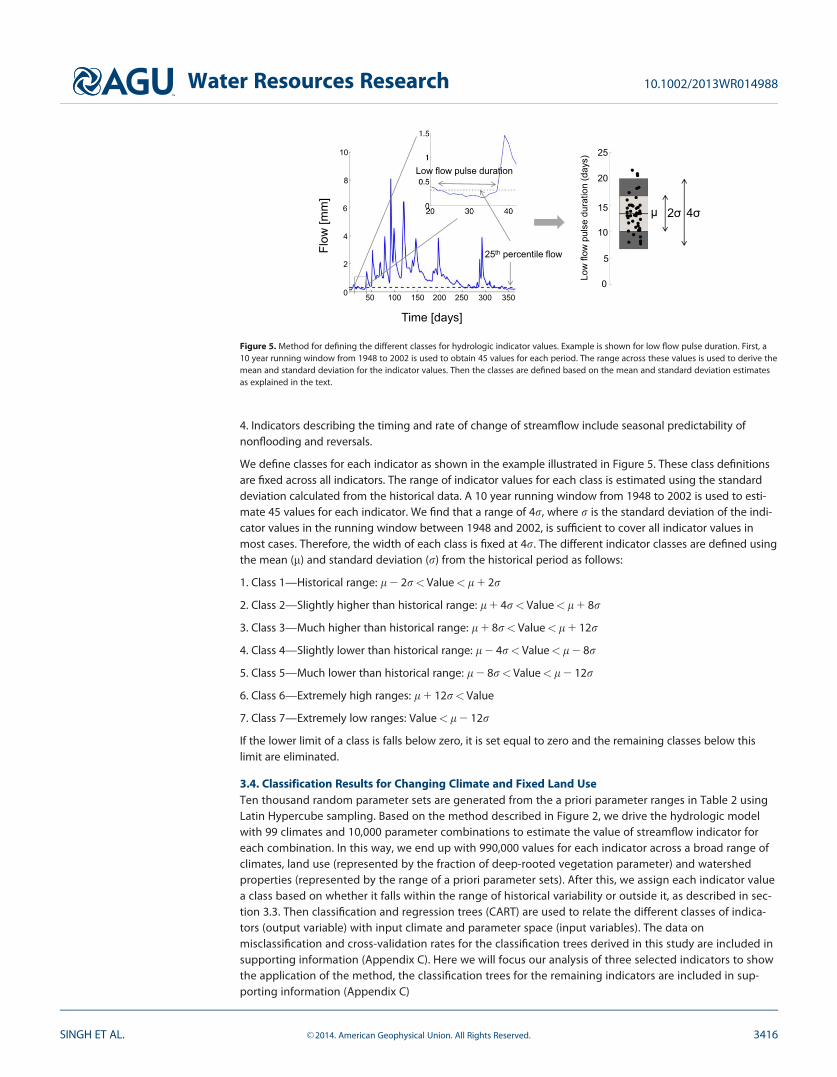
We define classes for each indicator as shown in the example illustrated in Figure 5. These class definitionsare fixed across all indicators. The range of indicator values for each class is estimated using the standarddeviation calculated from the historical data. A 10 year running window from 1948 to 2002 is used to esti-mate 45 values for each indicator. We find that a range of 4r, where r is the standard deviation of the indi-cator values in the running window between 1948 and 2002, is sufficient to cover all indicator values inmost cases. Therefore, the width of each class is fixed at 4r. The different indicator classes are defined usingthe mean (m) and standard deviation (r) from the historical period as follows:

1. Class 1—Historical range: l 2 2r<Value< l 1 2r

2. Class 2—Slightly higher than historical range: l 1 4r< Value< l 1 8r

3. Class 3—Much higher than historical range: l 1 8r< Value<l 1 12r

4. Class 4—Slightly lower than historical range: l 2 4r< Value< l 2 8r

5. Class 5—Much lower than historical range: l 2 8r< Value<l 2 12r

6. Class 6—Extremely high ranges: l 1 12r<Value

7. Class 7—Extremely low ranges: Value<l 2 12r

If the lower limit of a class is falls below zero, it is set equal to zero and the remaining classes below thislimit are eliminated.

3.4. Classification Results for Changing Climate and Fixed Land UseTen thousand random parameter sets are generated from the a priori parameter ranges in Table 2 usingLatin Hypercube sampling. Based on the method described in Figure 2, we drive the hydrologic modelwith 99 climates and 10,000 parameter combinations to estimate the value of streamflow indicator foreach combination. In this way, we end up with 990,000 values for each indicator across a broad range ofclimates, land use (represented by the fraction of deep-rooted vegetation parameter) and watershedproperties (represented by the range of a priori parameter sets). After this, we assign each indicator valuea class based on whether it falls within the range of historical variability or outside it, as described in sec-tion 3.3. Then classification and regression trees (CART) are used to relate the different classes of indica-tors (output variable) with input climate and parameter space (input variables). The data onmisclassification and cross-validation rates for the classification trees derived in this study are included insupporting information (Appendix C). Here we will focus our analysis of three selected indicators to showthe application of the method, the classification trees for the remaining indicators are included in sup-porting information (Appendix C)

Low flow pulse duration

25th percentile flow

Low

flow

pul

se d

urat

ion

(day

s)

4σ2σμ

Flow

[mm

]Time [days]

50 100 150 200 250 300 3500

2

4

6

8

10 25

20

15

10

5

0

Figure 5. Method for defining the different classes for hydrologic indicator values. Example is shown for low flow pulse duration. First, a10 year running window from 1948 to 2002 is used to obtain 45 values for each period. The range across these values is used to derive themean and standard deviation for the indicator values. Then the classes are defined based on the mean and standard deviation estimatesas explained in the text.



1. Mean annual runoff: This indicator represents general water availability

2. Maximum August flow: August is a month of low flows and this indicator suggests the condition of lowflows

3. Flood frequency: Indicates the condition of high flows.

We start with the controls on flood frequency for the case of changing climates but fixed land use. In thiscase, the fraction of deep-rooted vegetation is fixed at the historical range. Figure 6a shows the differentclass assignments based on historical variability of flood frequency derived from streamflow data. Class defi-nitions have been provided in section 3.3. Here we assume that an increase (shown by yellow and shadesof red) in the value of the flood frequency will lead to vulnerability since that corresponds to the watershedexperiencing high floods more frequently, a decrease is assumed to have uncertain impacts (shown byshades of green).

Figure 6b shows the classification tree for flood frequency for fixed land use but changing climates. Thetree consists of many nodes, each of which is a logical expression. If the expression is true, the left branch isfollowed, otherwise the right one. In this manner, by navigating different subspaces of climate and parame-ters, we reach a ‘‘terminal’’ node or a leaf. At the leaf, the indicator class that results from the combinationof different logical expressions is shown. From the tree in Figure 6b, we find that the primary control on thisindicator is precipitation (shown as Pratio—the ratio of mean annual precipitation in the future to historicalmean annual precipitation) followed by the recession coefficient describing the recession from the subsur-face soil moisture store (Ass). The maximum height of soil moisture storage (Sb) is the third control. Thissuggests that frequency of high floods depends first upon the climate of the watershed followed by its abil-ity to release water from the subsurface and amount of water that can be stored in the subsurface.

We also show the class probabilities associated with the classes 1–7. This gives an indication of how ‘‘pure’’a terminal node is. If all the indicator values based on navigating a set of logical expressions resulted in asingle class, the probability distribution will be skewed toward that class. On the other extreme, if the classi-fication algorithm is unable to relate the indicators class with specific regions in the input variables space,the node will be highly impure, or the probability distribution across classes 1–7 will be nearly flat. Most ofthe times the probability distribution are in the middle of these two extremes suggesting there is alwayssome uncertainty in threshold values of climate and parameters selected by the classification algorithm.

Using Figure 6b, one can also identify the different pathways that lead to vulnerability of the indicator asshown by solid black lines. Even for small rises in mean annual precipitation (increase of 5% from historicalvalue) the indicator can transition to different dominant controls. In this case, if the mean annual

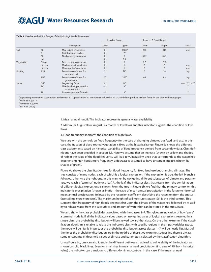
Table 2. Feasible and A Priori Ranges of the Hydrologic Model Parameters

Description

Feasible Range Reduced A Priori Rangea

UnitsLower Upper Lower Upper

Soil Sb Max height of soil store 0 2000b 290 810 mmB Distribution of buckets 0 7b

FC Field capacity parameter 0 1 0.22 0.43Kd 0 0.5c

Vegetation %Veg Deep-rooted vegetation 0 1 0.6 0.8LAImax Maximum leaf area index 0 6 0 6 mmLAImin Minimum leaf area index 0 6 0 6 mm

Routing ASS Recession coefficient forsaturated soil

1 20d 6 14 days

ABF Recession coefficient forgroundwater

20 200d 40 83 days

Snow Ddf Degree day factor 0 20b mm �C21 d21

Tth Threshold temperature forsnow formation

25 5b �C

Tb Base temperature for melt 25 5b �C

aSupporting information (Appendix B) and section 3.1. Upper limit of FC was further reduced as FC >0.43 did not produce realistic flows for the observed hydrograph.bKollat et al. [2013].cFarmer et al. [2003].dBai et al. [2009].



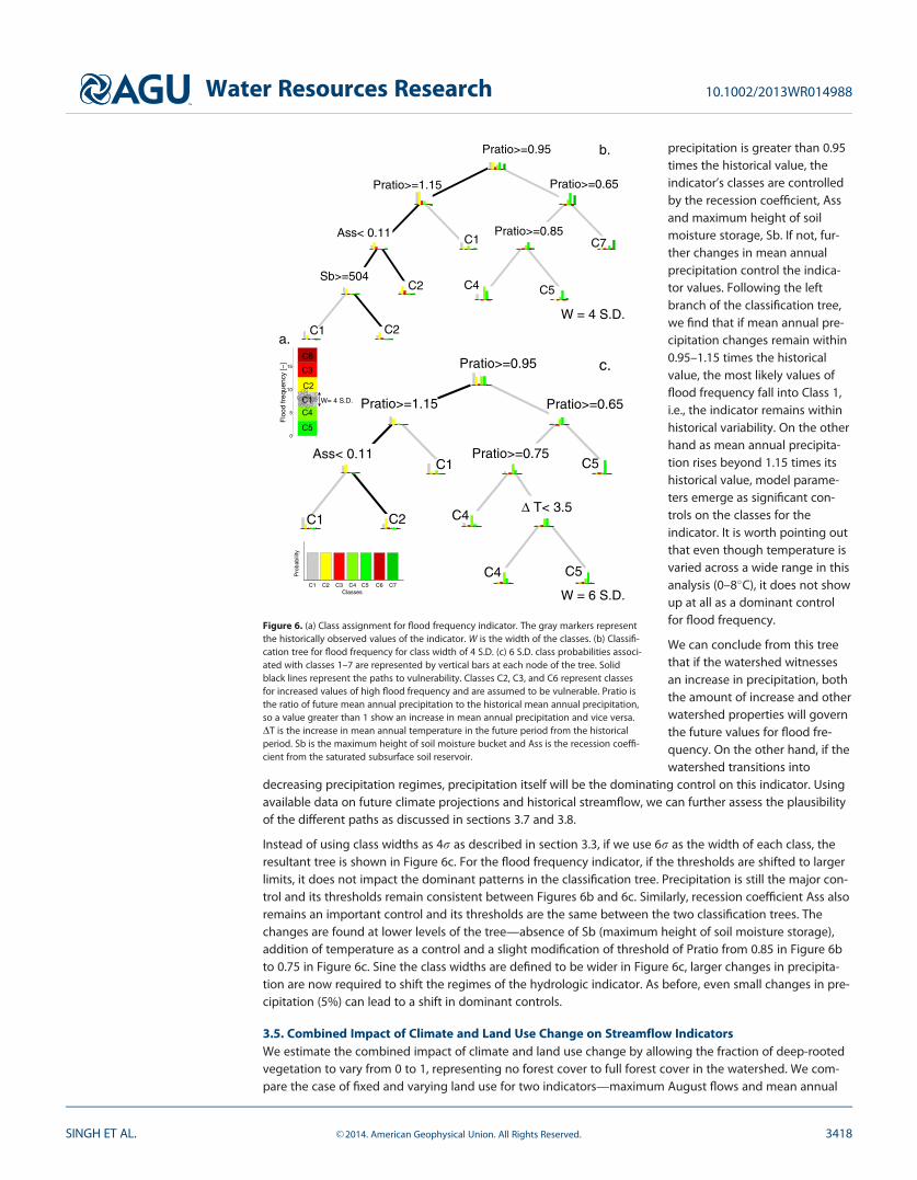
precipitation is greater than 0.95times the historical value, theindicator’s classes are controlledby the recession coefficient, Assand maximum height of soilmoisture storage, Sb. If not, fur-ther changes in mean annualprecipitation control the indica-tor values. Following the leftbranch of the classification tree,we find that if mean annual pre-cipitation changes remain within0.95–1.15 times the historicalvalue, the most likely values offlood frequency fall into Class 1,i.e., the indicator remains withinhistorical variability. On the otherhand as mean annual precipita-tion rises beyond 1.15 times itshistorical value, model parame-ters emerge as significant con-trols on the classes for theindicator. It is worth pointing outthat even though temperature isvaried across a wide range in thisanalysis (0–8�C), it does not showup at all as a dominant controlfor flood frequency.

We can conclude from this treethat if the watershed witnessesan increase in precipitation, boththe amount of increase and otherwatershed properties will governthe future values for flood fre-quency. On the other hand, if thewatershed transitions into

decreasing precipitation regimes, precipitation itself will be the dominating control on this indicator. Usingavailable data on future climate projections and historical streamflow, we can further assess the plausibilityof the different paths as discussed in sections 3.7 and 3.8.

Instead of using class widths as 4r as described in section 3.3, if we use 6r as the width of each class, theresultant tree is shown in Figure 6c. For the flood frequency indicator, if the thresholds are shifted to largerlimits, it does not impact the dominant patterns in the classification tree. Precipitation is still the major con-trol and its thresholds remain consistent between Figures 6b and 6c. Similarly, recession coefficient Ass alsoremains an important control and its thresholds are the same between the two classification trees. Thechanges are found at lower levels of the tree—absence of Sb (maximum height of soil moisture storage),addition of temperature as a control and a slight modification of threshold of Pratio from 0.85 in Figure 6bto 0.75 in Figure 6c. Sine the class widths are defined to be wider in Figure 6c, larger changes in precipita-tion are now required to shift the regimes of the hydrologic indicator. As before, even small changes in pre-cipitation (5%) can lead to a shift in dominant controls.

3.5. Combined Impact of Climate and Land Use Change on Streamflow IndicatorsWe estimate the combined impact of climate and land use change by allowing the fraction of deep-rootedvegetation to vary from 0 to 1, representing no forest cover to full forest cover in the watershed. We com-pare the case of fixed and varying land use for two indicators—maximum August flows and mean annual

Pratio>=0.95

Pratio>=1.15 Pratio>=0.65

Ass< 0.11 C1

Sb>=504

C1 C2

C2

Pratio>=0.85

C4 C5

C7

Pratio>=0.95


Ass< 0.11

C1 C2

C1Pratio>=0.75

C4

C5

Δ T< 3.5

C4 C5

0

5

10

15

Flo

od fr

eque

ncy

[−]

W= 4 S.D.

C1 C2 C3 C4 C5 C6 C7Classes

Pro

babi

lity

W = 4 S.D.

W = 6 S.D.

a.

b.

c.C6C3

C2C1C4

C5

Figure 6. (a) Class assignment for flood frequency indicator. The gray markers representthe historically observed values of the indicator. W is the width of the classes. (b) Classifi-cation tree for flood frequency for class width of 4 S.D. (c) 6 S.D. class probabilities associ-ated with classes 1–7 are represented by vertical bars at each node of the tree. Solidblack lines represent the paths to vulnerability. Classes C2, C3, and C6 represent classesfor increased values of high flood frequency and are assumed to be vulnerable. Pratio isthe ratio of future mean annual precipitation to the historical mean annual precipitation,so a value greater than 1 show an increase in mean annual precipitation and vice versa.DT is the increase in mean annual temperature in the future period from the historicalperiod. Sb is the maximum height of soil moisture bucket and Ass is the recession coeffi-cient from the saturated subsurface soil reservoir.



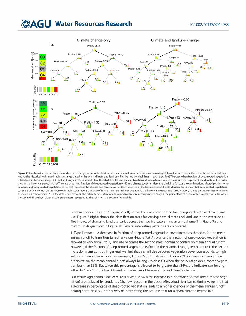
flows as shown in Figure 7. Figure 7 (left) shows the classification tree for changing climate and fixed landuse, Figure 7 (right) shows the classification trees for varying both climate and land use in the watershed.The impact of changing land use varies across the two indicators—mean annual runoff in Figure 7a andmaximum August flow in Figure 7b. Several interesting patterns are discovered

1. Type I impact—A decrease in fraction of deep-rooted vegetation cover increases the odds for the meanannual runoff to transition to higher values (Figure 7a). Also once the fraction of deep-rooted vegetation isallowed to vary from 0 to 1, land use becomes the second most dominant control on mean annual runoff.However, if the fraction of deep-rooted vegetation is fixed in the historical range, temperature is the secondmost dominant control. In general, we find that a small deep-rooted vegetation cover corresponds to highvalues of mean annual flow. For example, Figure 7a(right) shows that for a 25% increase in mean annualprecipitation, the mean annual runoff always belongs to class C3 when the percentage deep-rooted vegeta-tion less than 36%. But when this percentage is allowed to be greater than 36%, the indicator can belongeither to Class 1 or in Class 2 based on the values of temperature and climate change.

Our results agree with Frans et al. [2013] who show a 5% increase in runoff when forests (deep-rooted vege-tation) are replaced by croplands (shallow rooted) in the upper Mississippi river basin. Similarly, we find thata decrease in percentage of deep-rooted vegetation leads to a higher chances of the mean annual runoffbelonging to class 3. Another way of interpreting this result is that for a given climatic regime in a

Climate change only Climate and land use change a.

b.

0.2

0.3

0.4

0.5

0.6

0.7

0.80

0.20.4

Pratio>=0.95

Pratio< 1.25 Pratio>=0.65

%Vg< 31

%Vg>=36

Pratio< 1.05

C1C2

Pratio>=1.05

C1

Δ T< 3.5C1

C4

Pratio< 1.35C3

Δ T>=2.5

C1

C2

C2

%Vg<25

%Vg< 31

C4 C5

Pratio>=0.75

C1 C4

C4

0 1

0.2

0.3

0.4

0.5

0.6

0.7

0.8

00.20.4

Pratio>=1.05


Pratio>=1.25 C2

Δ T>=2.5

C1 C2

C1

Pratio>=0.75

C5

Pratio>=0.95 Δ T< 4.5

C4C5

Δ T< 2.5

C1 C4

C4

250

500

750

1000

Mea

n an

nual

run

off[m

m/y

r]

C3

C2

C1

C4C5

C1 C2 C3 C4 C5Pro

babi

lity

00.20.4 Pratio>=0.85


%Vg>=32

C1

%Vg>=43

%Vg>=13

C2 C5

Pratio< 1.35C5

Sb>=463

C2 C5

%Vg<34

C1 C4

C4

C5

0.2

0.3

0.4

0.5

0.6

0.7

0.8

00.20.4 Pratio>=0.85


B>=0.91 Pratio< 1.35

Sb>=455

C1

C4

Pratio< 0.95

C1 C2

Sb>=493 Sb>=559

C3 C5 B<1.3

C1 C2

C3

Sb< 493

C1 C4

C4

C1C2C3C4C5Pro

babi

lity

0 6 0 7 0 80

0.5

1

1.5

2

2.5

3

3.5

Max

imum

aug

ust f

low

[mm

/day

]

C5

C3

C4

C1

C2

Figure 7. Combined impact of land use and climate change in the watershed for (a) mean annual runoff and (b) maximum August flow. For both cases, there is only one path that canlead to the historically observed indicator range based on historical climate and land use, highlighted by black lines in each tree. (left) The case when fraction of deep-rooted vegetationis fixed within historical range (0.6–0.8) and only climate is varied. Here the black line follows the combinations of precipitation and temperature that represent the climate of the water-shed in the historical period. (right) The case of varying fraction of deep-rooted vegetation (0–1) and climate together. Here the black line follows the combinations of precipitation, tem-perature, and deep-rooted vegetation cover that represent the climate and forest cover of the watershed in the historical period. Both decision trees show that deep-rooted vegetationcover is a critical control on the hydrologic indicator. Pratio is the ratio of future mean annual precipitation to the historical mean annual precipitation, so a value greater than one showsan increase and vice versa. DT is the difference between the future temperature and historical mean annual temperature. %Vg is the percentage of deep-rooted vegetation in the water-shed. B and Sb are hydrologic model parameters representing the soil moisture accounting module.



watershed, the input precipitation (P) is partitioned into green (ET) and blue water (Q) on the basis of extentof deep-rooted vegetation cover. So an increase in one will logically lead to a decrease in other.

2. Type II impact—A high fraction of deep-rooted vegetation cover is the only way some indicators canmaintain their historically observed ranges. Maximum August flows would be much higher (belonging toclasses 2, or class 5) than its historically observed range (Class 1) if the percentage of deep-rooted vegeta-tion in the watershed decreased beyond 32% (Figure 7b, right).

3. Type III impact—Deep-rooted vegetation cover interacts with climate to generate different possible statesfor the watershed. For example, keeping the percentage of deep-rooted vegetation in the watershed above43% may prevent extreme increases in maximum August flows. If the vegetation falls below 44% the maxi-mum August flows will always belong to class 5 (Figure 7b, right). The classification trees for combined cli-mate and land use change show how these two types of changes interact with each other to generatedifferent regimes for a hydrologic indicator.

In general, we find that until deep-rooted vegetation in the watershed falls below 50%, it will not become amajor factor on controlling the different hydrologic indicators since the split values in logical expressionsfor fraction of deep-rooted vegetation picked by CART is less than 50% in almost all cases. On the otherhand, even small changes in precipitation (�5%) significantly impact the dominant controls on the indica-tor. For the classification trees showing the impact of deep-rooted vegetation for other hydrologic indica-tors, see supporting information (Appendix C, Figures C1–C6).

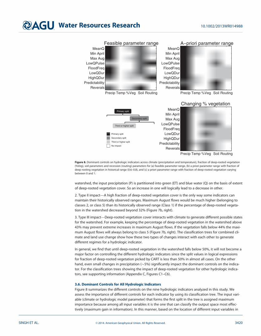
3.6. Dominant Controls for All Hydrologic IndicatorsFigure 8 summarizes the different controls on the nine hydrologic indicators analyzed in this study. Weassess the importance of different controls for each indicator by using its classification tree. The input vari-able (climate or hydrologic model parameter) that forms the first split in the tree is assigned maximumimportance because among all input variables it is the one that can classify the output space most effec-tively (maximum gain in information). In this manner, based on the location of different input variables in

Precip Temp %Veg Soil Routing

MeanQMin AprilMax Aug

LowQPulseFloodFreqLowQDurHighQDur

PredictabilityReverals









Changing % vegetation

Feasible parameter range A−priori parameter range

Primary split

Secondary split

Third or higher split

Primary split

Secondary split

Third or higher split

No impact

Figure 8. Dominant controls on hydrologic indicators across climate (precipitation and temperature), fraction of deep-rooted vegetation(%Veg), soil parameters and recession (routing) parameters for (a) feasible parameter range, (b) a priori parameter range with fraction ofdeep rooting vegetation in historical range (0.6–0.8), and (c) a priori parameter range with fraction of deep-rooted vegetation varyingbetween 0 and 1.



the tree, we assign them a relative importance. This assignment is depicted by different shades of gray andis shown in the legend in Figure 8. We show these controls for three cases—when parameters vary acrosstheir entire feasible range, parameters are fixed at their a priori ranges, all parameters except the fraction ofdeep-rooted vegetation cover are fixed at their a priori ranges (the case of varying land use).

We observe that the controls vary across indicators. Across the entire feasible ranges of parameters, formagnitude-related indicators, climate is the primary control, soil parameters are the secondary control andvegetation together with recession (or routing) parameters are tertiary controls. The recession parametersare not important at all for two out of three magnitude-related indicators. For flood frequency, climate andsoil parameters are dominant, whereas recession parameters are most important for low flow pulse count.For low flow pulse duration, precipitation is the dominant control followed by soil, vegetation, and reces-sion parameters. On the other hand, high flow pulse duration is mainly governed by the recession parame-ters; climate has a secondary effect and vegetation with soil parameters have a tertiary effect. For rate ofchange indicator (reversals), soil parameters are the important controls followed by vegetation and climate.No statistically significant trees are obtained for seasonal predictability of nonflooding in the case of feasibleparameter ranges.

When we reduce the feasible space to a priori ranges of hydrologic model parameters based on watershedphysical properties, temperature shows up as an important secondary control for two out of threemagnitude-related indicators. For magnitude-related indicators, climate is the dominant control with bothprecipitation and temperature being present in the classification tree. For monthly flows (minimum Apriland maximum August), soil parameters also have tertiary importance. For low flow pulse count, climate andsoil parameters (deep recharge coefficient and soil shape parameter) are important. For flood frequency, cli-mate is the primary control (also seen in detail in Figure 6) followed by recession and soil parameters. Forduration-related indicators too, climate followed by recession and soil parameters are the main controls.The controls for rate of change (reversal) are similar as the case of feasible space with climate becoming themost important in restricted parameter space. The predictability of nonflooding is governed mainly by soilparameters followed by climate. However, this tree has a very skewed distribution with most of the indica-tor values belonging to the historical class (root node in Figure C5) and therefore the classification is notreliable. Once we allow the fraction of deep-rooted vegetation in the watershed to vary from 0 to 1 (thecase of changing percentage vegetation), land use turns out to be the secondary control across all indica-tors. It is particularly important for low flow pulse count, low flow pulse duration, timing and rate-relatedindicators.

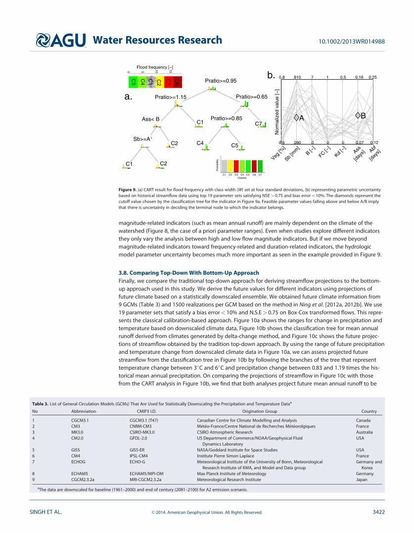
3.7. Impact of Parametric Uncertainty When Navigating the Classification TreesIn order to ascertain which path in a classification tree the watershed will follow, we need estimates ofmodel parameters. Figure 9a shows classification tree for flood frequency (section 3.4 and Figure 6) basedon a range of climates, fraction of deep-rooted vegetation fixed at historical ranges, and a priori ranges ofparameters. A further reduced range of values for important parameters selected on the basis of calibrationare shown in Figure 9b. Out of 10,000 parameter sets generated using uniform random sampling, 19 param-eter sets satisfying Nash-Sutcliffe Efficiency (N.S.E)> 0.75 on Box-Cox transformed flows (using a Box-Coxparameter value of 0.3) and absolute bias error< 10% are chosen to represent the range of parametricuncertainty [Nash and Sutcliffe, 1970; Brazil, 1988; Kottegoda and Rosso, 1997]. The Nash-Sutcliffe Efficiencywas estimated for daily time steps and the absolute bias error was estimated as the difference betweentotal runoff simulated and observed across the 10 year period.

Even across a relatively small set of high performing parameter sets, the ranges of parameters are high.High parametric uncertainty blurs the differentiation between the plausibility of different paths. We findthat high uncertainty in recession coefficient, Ass, leads to two paths being feasible while analyzing theregion of space with increases in precipitation beyond 15% of the historical value. This indicates the needfor reducing these uncertainties in order to decrease the range of possible futures. The tree also demon-strates how uncertainties in climate and parameters interact with each other in a complex manner. Even ifwe know for certain the future climate, existing parameter uncertainties makes the projection of futureregime of indicator uncertain.

We generally do not observe such an impact of hydrologic model parameters on estimates of hydrologicindicators in other studies since they focus mainly on magnitude-related indicators. In this study too, the



magnitude-related indicators (such as mean annual runoff) are mainly dependent on the climate of thewatershed (Figure 8, the case of a priori parameter ranges). Even when studies explore different indicatorsthey only vary the analysis between high and low flow magnitude indicators. But if we move beyondmagnitude-related indicators toward frequency-related and duration-related indicators, the hydrologicmodel parameter uncertainty becomes much more important as seen in the example provided in Figure 9.

3.8. Comparing Top-Down With Bottom-Up ApproachFinally, we compare the traditional top-down approach for deriving streamflow projections to the bottom-up approach used in this study. We derive the future values for different indicators using projections offuture climate based on a statistically downscaled ensemble. We obtained future climate information from9 GCMs (Table 3) and 1500 realizations per GCM based on the method in Ning et al. [2012a, 2012b]. We use19 parameter sets that satisfy a bias error< 10% and N.S.E> 0.75 on Box-Cox transformed flows. This repre-sents the classical calibration-based approach. Figure 10a shows the ranges for change in precipitation andtemperature based on downscaled climate data, Figure 10b shows the classification tree for mean annualrunoff derived from climates generated by delta-change method, and Figure 10c shows the future projec-tions of streamflow obtained by the tradition top-down approach. By using the range of future precipitationand temperature change from downscaled climate data in Figure 10a, we can assess projected futurestreamflow from the classification tree in Figure 10b by following the branches of the tree that representtemperature change between 3�C and 6�C and precipitation change between 0.83 and 1.19 times the his-torical mean annual precipitation. On comparing the projections of streamflow in Figure 10c with thosefrom the CART analysis in Figure 10b, we find that both analyses project future mean annual runoff to be

Table 3. List of General Circulation Models (GCMs) That Are Used for Statistically Downscaling the Precipitation and Temperature Dataa

No Abbreviation CMIP3 I.D. Origination Group Country

1 CGCM3.1 CGCM3.1 (T47) Canadian Centre for Climate Modelling and Analysis Canada2 CM3 CNRM-CM3 M�et�eo-France/Centre National de Recherches M�et�eorolgiques France3 MK3.0 CSIRO-MK3.0 CSIRO Atmospheric Research Australia4 CM2.0 GFDL-2.0 US Department of Commerce/NOAA/Geophysical Fluid

Dynamics LaboratoryUSA

5 GISS GISS-ER NASA/Goddard Institute for Space Studies USA6 CM4 IPSL-CM4 Institute Pierre Simon Laplace France7 ECHOG ECHO-G Meteorological Institute of the University of Bonn, Meteorological

Research Institute of KMA, and Model and Data groupGermany and

Korea8 ECHAM5 ECHAM5/MPI-OM Max Planck Institute of Meteorology Germany9 CGCM2.3.2a MRI-CGCM2.3.2a Meteorological Research Institute Japan

aThe data are downscaled for baseline (1961–2000) and end of century (2081–2100) for A2 emission scenario.

Nor

mal

ized

val

ue [−

]

Veg [%

]

Sb [m

m]

B [−]

FC [−]

Kd [−

]Ass

[day

s] Abf

[day

s]

0.6 0 0

0.250.160.517810

290 0 0.07 0.12

0.8

a.

b.

Sb>=A

Pratio>=0.95


Ass< B C1

Sb>=A

C1 C2

C2

Pratio>=0.85

C4 C5

C7A B

C1 C2 C3 C4 C5 C6 C7Classes

Pro

babi

lity

00

06

00 5 10 15

Flood frequency [−]

C6

C3C2

C1

C4

C5

Figure 9. (a) CART result for flood frequency with class width (W) set at four standard deviations, (b) representing parametric uncertaintybased on historical streamflow data using top 19 parameter sets satisfying NSE> 0.75 and bias error< 10%. The diamonds represent thecutoff value chosen by the classification tree for the indicator in Figure 9a. Feasible parameter values falling above and below A/B implythat there is uncertainty in deciding the terminal node to which the indicator belongs.



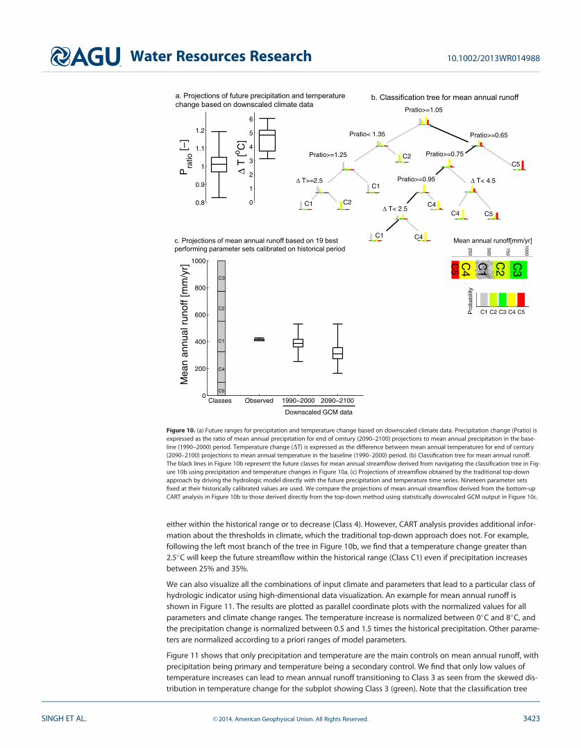
either within the historical range or to decrease (Class 4). However, CART analysis provides additional infor-mation about the thresholds in climate, which the traditional top-down approach does not. For example,following the left most branch of the tree in Figure 10b, we find that a temperature change greater than2.5�C will keep the future streamflow within the historical range (Class C1) even if precipitation increasesbetween 25% and 35%.

We can also visualize all the combinations of input climate and parameters that lead to a particular class ofhydrologic indicator using high-dimensional data visualization. An example for mean annual runoff isshown in Figure 11. The results are plotted as parallel coordinate plots with the normalized values for allparameters and climate change ranges. The temperature increase is normalized between 0�C and 8�C, andthe precipitation change is normalized between 0.5 and 1.5 times the historical precipitation. Other parame-ters are normalized according to a priori ranges of model parameters.

Figure 11 shows that only precipitation and temperature are the main controls on mean annual runoff, withprecipitation being primary and temperature being a secondary control. We find that only low values oftemperature increases can lead to mean annual runoff transitioning to Class 3 as seen from the skewed dis-tribution in temperature change for the subplot showing Class 3 (green). Note that the classification tree

2.5 3 3.50.8

0.9

1

1.1

1.2

Pra

tio [−

]

2.5 3 3.50

1

2

3

4

5

6

Δ T

[o C]

0 1

0.2

0.3

0.4

0.5

0.6

0.7

0.8

00.20.4

Pratio>=1.05


Pratio>=1.25 C2

Δ T>=2.5

C1 C2

C1

Pratio>=0.75

C5

Pratio>=0.95 Δ T< 4.5

C4C5

Δ T< 2.5

C1 C4

C4

Classes Observed 1990−2000 2090−21000

200

400

600

800

1000

Mea

n an

nual

run

off [

mm

/yr]

C3

C2

C1

C4

C5

Downscaled GCM data

C1 C2 C3 C4 C5Pro

babi

lity

250

500

750

1000

Mean annual runoff[mm/yr]

C3

C2

C1

C4

C5

a. Projections of future precipitation and temperature change based on downscaled climate data

c. Projections of mean annual runoff based on 19 best performing parameter sets calibrated on historical period

b. Classification tree for mean annual runoff

Figure 10. (a) Future ranges for precipitation and temperature change based on downscaled climate data. Precipitation change (Pratio) isexpressed as the ratio of mean annual precipitation for end of century (2090–2100) projections to mean annual precipitation in the base-line (1990–2000) period. Temperature change (DT) is expressed as the difference between mean annual temperatures for end of century(2090–2100) projections to mean annual temperature in the baseline (1990–2000) period. (b) Classification tree for mean annual runoff.The black lines in Figure 10b represent the future classes for mean annual streamflow derived from navigating the classification tree in Fig-ure 10b using precipitation and temperature changes in Figure 10a. (c) Projections of streamflow obtained by the traditional top-downapproach by driving the hydrologic model directly with the future precipitation and temperature time series. Nineteen parameter setsfixed at their historically calibrated values are used. We compare the projections of mean annual streamflow derived from the bottom-upCART analysis in Figure 10b to those derived directly from the top-down method using statistically downscaled GCM output in Figure 10c.



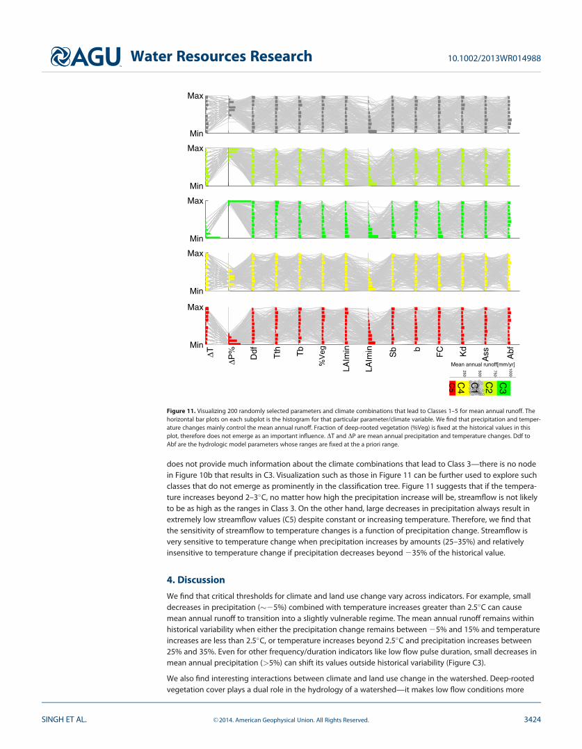
does not provide much information about the climate combinations that lead to Class 3—there is no nodein Figure 10b that results in C3. Visualization such as those in Figure 11 can be further used to explore suchclasses that do not emerge as prominently in the classification tree. Figure 11 suggests that if the tempera-ture increases beyond 2–3�C, no matter how high the precipitation increase will be, streamflow is not likelyto be as high as the ranges in Class 3. On the other hand, large decreases in precipitation always result inextremely low streamflow values (C5) despite constant or increasing temperature. Therefore, we find thatthe sensitivity of streamflow to temperature changes is a function of precipitation change. Streamflow isvery sensitive to temperature change when precipitation increases by amounts (25–35%) and relativelyinsensitive to temperature change if precipitation decreases beyond 235% of the historical value.

4. Discussion

We find that critical thresholds for climate and land use change vary across indicators. For example, smalldecreases in precipitation (�25%) combined with temperature increases greater than 2.5�C can causemean annual runoff to transition into a slightly vulnerable regime. The mean annual runoff remains withinhistorical variability when either the precipitation change remains between 25% and 15% and temperatureincreases are less than 2.5�C, or temperature increases beyond 2.5�C and precipitation increases between25% and 35%. Even for other frequency/duration indicators like low flow pulse duration, small decreases inmean annual precipitation (>5%) can shift its values outside historical variability (Figure C3).

We also find interesting interactions between climate and land use change in the watershed. Deep-rootedvegetation cover plays a dual role in the hydrology of a watershed—it makes low flow conditions more

Min

Max

Min

Max

Min

Max

Min

Max

250

500

750

1000

Mean annual runoff[mm/yr]

C3

C2

C1

C4

C5

Min

Max

ΔT

ΔP%

Ddf Tth Tb

LAIm

in

LAIm

in

Sb b

FC Kd

Ass Abf

%V

eg

Figure 11. Visualizing 200 randomly selected parameters and climate combinations that lead to Classes 1–5 for mean annual runoff. Thehorizontal bar plots on each subplot is the histogram for that particular parameter/climate variable. We find that precipitation and temper-ature changes mainly control the mean annual runoff. Fraction of deep-rooted vegetation (%Veg) is fixed at the historical values in thisplot, therefore does not emerge as an important influence. DT and DP are mean annual precipitation and temperature changes. Ddf toAbf are the hydrologic model parameters whose ranges are fixed at the a priori range.



severe due to larger evapotranspiration, but also mediates the impacts of high flows. For example, the clas-sification tree showing the controls on low flow pulse duration with varying fraction of deep-rooted vegeta-tion (Figure C3, bottom) illustrates that for all cases of mean annual precipitation decreases between 235%and 215% of the historical value, and percentages of deep-rooted vegetation less than 36%, the indicatorhas high probability of belonging to the slightly vulnerable class—Class C2. But for the same range of meanannual precipitation, if the percentage of deep-rooted vegetation is greater than 36%, the indicator hashigher chances of belonging to much higher vulnerability classes—C3 and C6. So an increase in percentageof deep-rooted vegetation leads to increased chances of persistence of low flow conditions in the stream.This is similar to a recent observation from four headwater catchments in central and Western Europe byTeuling et al. [2013], where they find that evapotranspiration intensified the summer drought in thesecatchments.

In another example, the case of mean annual runoff in Figure 7a (case of combined climate and land usechange), we find that for increases in mean annual precipitation greater than 25%, the likelihood of themean annual runoff belonging to extremely high values (Class C3) is greatest if the percentage of deep-rooted vegetation in the watershed is less than 36%. If the percentage of vegetation is greater than 36%,depending on particular climate and temperature changes, the indicator values may fall in the historicallyobserved ranges or be slightly higher than historically observed values (Class C1 or C2).

5. Conclusions

In this study, we develop a vulnerability-based approach to quantify the impact of climate and land usechange on several streamflow indicators while considering hydrologic model parameter uncertainty. Weexplore a large space of climates, land uses and hydrologic model parameters, in order to understand theirrelative control on selected streamflow indicators, and find that different controls emerge across indicators.We also find that the sensitivity of streamflow to temperature and precipitation change depends upon themagnitude of the precipitation change itself. For example, the values of mean annual runoff are relativelyinsensitive to temperature change if mean annual precipitation decreases beyond 235% of the historicalvalue. The classification trees produced demonstrate that climate, soils, vegetation, and geomorphology(recession) come together in a complex manner to generate different streamflow regimes and characteris-tics. For each indicator, the different branches of the tree represent different states for the watershed result-ing from combinations of climate and physical characteristics.

There are three possible ways in which the bottom-up approach can assist the decision maker. First, thedetection of dominant controls on a hydrologic indicator helps the stakeholder to assess where investmentsshould be made to attempt to reduce uncertainties. For example, it is clear from the classification tree ofmean annual runoff that the reduction in uncertainty associated with future precipitation is very important.Second, the values of adverse climate and land use thresholds provide the decision maker with an indica-tion of how robust a watershed is to changing conditions. If small changes in climate/land use cause a tran-sition to vulnerable regimes, a highly risk averse strategy should be followed to tackle such potential futurechange. Third, studies focusing on impact of climate change on water resources generally neglect the roleof land use change while both are likely to occur concurrently in watersheds. We provide one way to com-bine both of these stressors in a common framework.

There are limitations in this study that allow for future improvements. First of all, the exploration of climatespace using the delta change method does not allow the stakeholder to analyze the impact of changingprecipitation characteristics beyond the mean amount (e.g., frequency of wet days) on the resultant stream-flow indicator. This limits our ability to test how precipitation changes will impact frequency characteristicsof streamflow. Use of weather generators that allow the variation in several hydrologically relevant charac-teristics of precipitation could reduce this problem in the future. Also the modeled impact of land usechange in our study is based on percentage of vegetation in the watershed and does not consider theimpact of changing leaf area indices on interception or other vegetation related hydrologic impacts.

We also show that the classification trees derived using this approach may show some dependence uponthe choice of vulnerability thresholds for the hydrologic indicators. Furthermore, the results presented hereare from as single model structure that leaves model structural uncertainty unaccounted for in our currentanalysis. However, the framework can potentially incorporate this uncertainty due to its ability to



incorporate categorical data that allows for inclusion of more than one model structures as separate catego-ries of input data. Finally, there can be large uncertainties (large misclassification error rates) in the classifi-cation trees themselves, indicating a complex control on the hydrologic indicator that is not easilysegregated by using CART. While we have addressed this issue by representing this uncertainty visually ashistograms at each leaf node, other classification methods (such as random forests) can be explored in thefuture for addressing such cases.

In summary, our method allows stakeholders to assess the vulnerability of a watershed to climate and landuse change within a hydrologic modeling framework. It provides a novel way to incorporate various sourcesof information about the watershed’s behavior to assess its response to changing climate or land use orboth. By combining the results of this approach with available climate projections, decisions makers will bebetter equipped to appraise different alternatives for future action.

ReferencesArnold, J. G., P. M. Allen, R. Muttiah, and G. Bernhardt (1995), Automated base flow separation and recession analysis techniques, Ground

Water, 33(6), 1010–1018, doi:10.1111/j.1746584.1995.tb00046.Bai, Y., T. Wagener, and P. Reed (2009), A top-down framework for watershed model evaluation and selection under uncertainty, Environ.

Modell. Software, 24, 901–916, doi:10.1016/j.envsoft.2008.12.012.Barron, E. J. (2009), Beyond climate science, Science, 326, 643.Bennett, K., A. Werner, and M. Schnorbus (2012), Uncertainties in hydrologic and climate change impact analyses in headwater basins of

British Columbia, J. Clim., 25(17), 5711–730, doi:10.1175/JCLI-D-11-00417.1.Beven, K. (2011), I believe in climate change but how precautionary do we need to be in planning the future?, Hydrol. Processes, 25, 1517–

1520, doi:10.1002/hyp.7939.Boso, F., F. P. J. de Barros, A. Fiori, and A. Bellin (2013), Performance analysis of statistical spatial measures for contaminant plume charac-

terization towards risk-based decision making, Water Resour. Res., 49, 3119–3132, doi:10.1002/wrcr.20270.Bosshard, T., M. Carambia, K. Goergen, S. Kotlarski, P. Krahe, M. Zappa, and C. Sch€a€ar (2013), Quantifying uncertainty sources in an ensem-

ble of hydrological climate-impact projections, Water Resour. Res., 49, 1523–1536, doi:10.1029/2011WR011533.Brazil, L. E. (1988), Multilevel calibration strategy for complex hydrologic simulation models, PhD thesis, Colo. State Univ., Fort Collins.Breiman, L., J. H. Friedman, R. A. Olshen, and C. J. Stone (1984), Classification and Regression Trees, Wadsworth and Brooks/Cole, Monterey,

Calif.Brown, C., W. Werick, W. Leger, and D. Fay (2011), A decision-analytic approach to managing climate risks: Application to the Upper Great

Lakes, J. Am. Water Resour. Assoc., 47(3), 524–534, doi:10.1111/j.1752-1688.2011.00552.x.Chen, J., F. P. Brissette, A. Poulin, and R. Leconte (2011), Overall uncertainty study of the hydrological impacts of climate change for a Cana-

dian watershed, Water Resour. Res., 47, W12509, doi:10.1029/2011WR010602.Christensen, J. H., et al. (2007), Regional Climate Projections, in Climate Change 2007: The Physical Science Basis, Contribution of Working

Group I to the Fourth Assessment Report of the Intergovernmental Panel on Climate Change, edited by S. Solomon et al., p. 856, CambridgeUniv. Press, Cambridge, New York.

Collins, M., R. E., Chandler, P. M. Cox, J. M. Huthnance, J. Rougier, and D. B. Stephenson (2012), Quantifying future climate change, Nat.Clim. Change, 2, 403–409, doi:10.1038/nclimate1414.

Dobler, C., S. Hagemann, R. L. Wilby, and J. St€otter (2012), Quantifying different sources of uncertainty in hydrological projections at thecatchment scale, Hydrol. Earth Syst. Sci. Discuss., 9, 8173–8211, doi:10.5194/hessd-9–8173-2012.

Duan, Q., et al. (2006), The Model Parameter Estimation Experiment (MOPEX): An overview of science strategy and major results from thesecond 20 and third workshops, J. Hydrol., 320(1–2), 3–17, doi:10.1016/j.jhydrol. 2005.07.031.

Falcone, J. A., D. M. Carlisle, D. M. Wolock, and M. R. Meador (2010), GAGES: A stream gage database for evaluating natural and altered flowconditions in the conterminous United States, Ecology, 91, 621.

Farmer, D., M. Sivapalan, and C. Jothityangkoon (2003), Climate, soil, and vegetation controls upon the variability of water balance in tem-perate and semiarid landscapes: Downward approach to water balance analysis, Water Resour. Res., 39(2), 1035, doi:10.1029/2001WR000328.

Frans, C., E. Istanbulluoglu, V. Mishra, F. Munoz-Arriola, and D. P. Lettenmaier (2013), Are climatic or land cover changes the dominantcause of runoff trends in the Upper Mississippi River Basin?, Geophys. Res. Lett., 40, 1104–1110, doi:10.1002/grl.50262.

Hall, J. (2007), Probabilistic climate scenarios may misrepresent uncertainty and lead to bad adaptation decisions, Hydrol. Processes, 21,1127–1129, doi:10.1002/hyp.6573.

Hargreaves, G. H., and Z. A. Samani (1985), Reference crop evapo-transpiration from temperature, Appl. Eng. Agric., 1(2), 96–99.Jones, R. N., H. S. C. Francis, W. C. Boughton, and L. Zhang (2006), Estimating sensitivity of mean annual runoff to climate change using

selected hydrologic models, Adv. Water Resour., 29, 1419–1429, doi:10.1016/j.advwatres.2005.11.001.Kapangaziwiri, E., D. A. Hughes, and T. Wagener (2012), Incorporating uncertainty in hydrological predictions for gauged and ungauged

basins in southern Africa, Hydrol. Sci. J., 57(5), 1000–1019.Kay, A. L., H. N. Davies, V. A. Bell, and R. G. Jones (2009), Comparison of uncertainty sources for climate change impacts: Flood frequency in

England, Clim. Change, 92(1–2), 41–63, doi:10.1007/s10584-008-9471-4.Khader, A. I., D. E. Rosenberg, and M. McKee (2013), A decision tree model to estimate the value of information provided by a groundwater

quality monitoring network, Hydrol. Earth. Syst. Sci., 17, 1797–1807, doi:10.5194/hess-17-1979-2013.Knutti, R., D. Masson, and A. Gettelman (2013), Climate model genealogy: Generation CMIP5 and how we got there, Geophys. Res. Lett., 40,

1194–1199, doi:10.1002/grl.50256.Kollat, J. B., P. M. Reed, and T. Wagener (2013), When are multiobjective calibration tradeoffs in hydrologic models meaningful?, Water

Resour. Res., 48, W03520, doi:10.1029/2011WR011534.Kottegoda, N. T., and R. Rosso (1997), Statistics, Probability and Reliability for Civil and Environmental Engineers, McGraw-Hill, New York.

AcknowledgmentsThis research was supported by theOffice of Science (BER), U.S.Department of Energy, grantDE-FG02–08ER64641 and an EPA STAREarly Career grant RD834196. Thiswork was partially supported by theNatural Environment Research Council(Consortium on Risk in theEnvironment: Diagnostics, Integration,Benchmarking, Learning and Elicitation(CREDIBLE); NE/J017450/1). All the dataused in the paper have been obtainedfrom free available sources cited in themanuscript.



Kunreuther, H., G. Heal, M. Allen, O. Edenhofer, C. B. Field, and G. Yohe (2013), Risk management and climate change, Nat. Clim. Change, 3,447–450, doi:10.1038/NCLIMATE1740.

Lempert, R. J., B. P. Bryant, and S. C. Bankes (2008), Comparing algorithms for scenario discovery, Working Pap. WR-557-NSF, RAND Corp.,Santa Monica, Calif.

Manning, L. J., J. W. Hall, H. J. Fowler, C. G. Kilsby, and C. Tebaldi (2009), Using probabilistic climate change information from a multimodelensemble for water resources assessment, Water Resour. Res., 45, W11411, doi:10.1029/2007WR006674.

Maurer, E. P., and P. B. Duffy (2005), Uncertainty in projections of streamflow changes due to climate change in California, Geophys. Res.Lett., 32, L03704, doi:10.1029/2004GL021462.

Merz, R., J. Parajka, and G. Bl€oschl (2010), Time stability of catchment model parameters: Implications for climate impact analyses, WaterResour. Res., 47, W02531, doi:10.1029/2010WR009505.

Milly, P. C. D., R. T. Wetherald, K. A. Dunne, and T. L. Delworth (2002), Increasing risk of great floods in a changing climate, Nature, 415, 514–517.

Milly, P.C.D, J. Betancourt, M. Falkenmark, R. M. Hirsch, Z.W. Kundzewicz, D.P. Lettenmaier, and R.J. Stouffer (2008), Stationarity is dead:Whither water management?, Science, 319(5863), 573–574, doi: 10.1126/science.1151915.

Moody, P., and C. Brown (2013), Robustness indicators for evaluation under climate change: Application to the Upper Great Lakes, WaterResour. Res., 49, 3576–3588, doi:10.1002/wrcr.20228.

Nash, J. E., and J. V. Sutcliffe (1970), River flow forecasting through conceptual models part I—A discussion of principles, J. Hydrol., 10(3),282–290.

Nash, L. L., and P. H. Gleick (1991), Sensitivity of streamflow in the Colorado basin to climatic changes, J. Hydrol., 125, 221–241, doi:10.1016/0022-1694(91)90030-L.

Ning, L., M. E. Mann, R. Crane, and T. Wagener (2012a), Probabilistic projections of climate change for the mid-Atlantic region of the UnitedStates: Validation of precipitation downscaling during the historical era, J. Clim., 25, 509–526, doi:10.1175/2011JCLI4091.1.

Ning, L., M. E. Mann, R. Crane, T. Wagener, R. G. Najjar Jr., and R. Singh (2012b), Probabilistic projections of climate change impacts on pre-cipitation for the mid-Atlantic region of the United States, J. Clim., 25, 509–526, doi:10.1175/2011JCLI4091.1.

Olden, J. D., and N. L. Poff (2003), Redundancy and the choice of hydrologic indices for characterizing streamflow regimes, River Res. Appl.,19, 101–121.

Paton, F. L., H. R. Maier, and G. C. Dandy (2013), Relative magnitudes of sources of uncertainty in assessing climate change impacts onwater supply security for the southern Adelaide water supply system, Water Resour. Res., 49, 1643–1667, doi:10.1002/wrcr.20153.

Prudhomme, C., and H. Davies (2009a), Assessing uncertainties in climate change impact analyses on the river flow regimes in the UK. Part1: Baseline climate, Clim. Change, 93, 177–195, doi:10.1007/s10584-008-9464-3.

Prudhomme, C., and H. Davies (2009b), Assessing uncertainties in climate change impact analyses on the river flow regimes in the UK. Part2: Future climate, Clim. Change, 93, 197–222, doi:10.1007/s10584-008-9461-6.

Sawicz, K. (2013), Catchment classification—Understanding hydrologic similarity through catchment function, PhD thesis, Pa. State Univ.,University Park.

Singh, R., T. Wagener, K. van Werkhoven, M. E. Mann, and R. Crane (2011), A trading-space-for-time approach to probabilistic continuousstreamflow predictions in a changing climate—Accounting for changing watershed behavior, Hydrol. Earth Syst. Sci., 15, 3591–3603,doi:10.5194/hess-13591-2011.

Singh, R., K. van Werkhoven, and T. Wagener (2013), Hydrologic impacts of climate change in gauged and ungauged watersheds of the Oli-fants Basin—A trading space-for-time approach, Hydrol. Sci. J., 59(1), 29–55, doi:10.1080/02626667.2013.819431.

Son, K., and M. Sivapalan (2007), Improving model structure and reducing parameter uncertainty in conceptual water balance modelsthrough the use of auxiliary data, Water Resour. Res., 43, W01415, doi:10.1029/2006WR005032.

Stephenson, D. B., M. Collins, J. C. Rougier, and R. E. Chandler (2012), Statistical problems in the probabilistic prediction of climate change,Environmetrics, 23(5), 364–372, doi:10.1002/env.2153.

Teng, J., J. Vaze, F. H. S. Chiew, B. Wang, and J.-M. Perraud (2012), Estimating the relative uncertainties sourced from GCMs and hydrologicalmodels in modeling climate change impact on runoff, J. Hydrometeorol., 13, 122–139, doi:10.1175/JHM-D-11-058.1.

Teuling, A. J., A. F. Van Loon, S. I. Seneviratne, I. Lehner, M. Aubinet, B. Heinesch, C. Bernhofer, T. Gr€unwald, H. Prasse, and U. Spank (2013),Evapotranspiration amplifies European summer drought, Geophys. Res. Lett., 40, 2071–2075, doi:10.1002/grl.50495.

Therneau, T. M., and E. J. Atkinson (1997), An introduction to recursive partitioning using the RPART routines, Tech. Rep. 61, Mayo Clinic,Division of Biostatistics, Rochester, Minn. [Available at http://www.mayo.edu/hsr/techrpt/61.pdf.]

Van Werkhoven, K., T. Wagener, P. Reed, and Y. Tang (2008), Characterization of watershed model behavior across a hydroclimatic gradi-ent, Water Resour. Res., 44, W01429, doi:10.1029/2007WR006271.

Wagener, T., M. Sivapalan, P. A. Troch, B. L. McGlynn, C. J. Harman, H. V. Gupta, P. Kumar, P. S. C. Rao, N. B. Basu, and J. S. Wilson (2010), Thefuture of hydrology: An evolving science for a changing world, Water Resour. Res., 46, W05301, doi:10.1029/2009WR008906.

Weaver, C. P., R. J. Lempert, C. Brown, J. A. Hall, D. Revell, and D. Sarewtiz (2013), Improving the contribution of climate model informationto decision making: The value and demands of robust decision frameworks, WIREs Clim. Change, 4, 39–60, doi:10.1002/wcc.202.

Wilby, R. L., and S. Dessai (2010), Robust adaptation to climate change, Weather, 65(7), 180–185, doi:10.1002/wea.543.Wilby, R. L., and I. Harris (2006), A framework for assessing uncertainties in climate change impacts: Low-flow scenarios for the River

Thames, UK, Water Resour. Res., 42, W02419, doi:10.1029/2005WR004065.Xu, C.-y., E. Wild�en, and S. Halldin (2005), Modelling hydrological consequences of climate change—Progress and challenges, Adv. Atmos.

Sci., 22(6), 789–797, doi:10.1007/BF02918679.Zhao, R. J., Y. L. Zhang, L. R. Fang, X. R. Liu, and Q. S. Zhang (1980), The Xinanjiang model, in Proceedings of the Symposium on the Applica-

tion of Recent Developments in Hydrological Forecasting to the Operation of Water Resource Systems, 129, pp. 351–356, IASH Publ., Oxford.



http://www.mayo.edu/hsr/techrpt/61.pdf

Documents

PUBLICATIONS - Penn State Meteo Computing … · Second, GCM projections have large uncertainties (depending upon the region) mainly due to parameter-ization of cloud physics, uncertainty