Embed Size (px)
Citation preview

JHEP11(2017)058
Published for SISSA by Springer
Received: April 10, 2017
Revised: August 19, 2017
Accepted: October 24, 2017
Published: November 10, 2017
Composite dark matter and Higgs
Yongcheng Wu,a,b,c Teng Ma,d Bin Zhanga,b and Giacomo Cacciapagliae
aDepartment of Physics, Tsinghua University,
Beijing, 100086, ChinabCenter for High energy Physics, Tsinghua University,
Beijing, 100084, ChinacOttawa-Carleton Institute for Physics, Carleton University,
Ottawa, Ontario K1S 5B6, CanadadCAS Key Laboratory of Theoretical Physics, Institute of Theoretical Physics,
Chinese Academy of Sciences, Beijing 100190, ChinaeUniv Lyon, Universite Lyon 1,
CNRS/IN2P3, IPNL, F-69622, Villeurbanne, France
E-mail: [email protected], [email protected],
[email protected], [email protected]
Abstract: We investigate the possibility that Dark Matter arises as a composite state
of a fundamental confining dynamics, together with the Higgs boson. We focus on the
minimal SU(4)×SU(4)/SU(4) model which has both a Dark Matter and a Higgs candidates
arising as pseudo-Nambu-Goldstone bosons. At the same time, a simple underlying gauge-
fermion theory can be defined providing an existence proof of, and useful constraints on,
the effective field theory description. We focus on the parameter space where the Dark
Matter candidate is mostly a gauge singlet. We present a complete calculation of its relic
abundance and find preferred masses between 500 GeV to a few TeV. Direct Dark Matter
detection already probes part of the parameter space, ruling out masses above 1 TeV, while
Indirect Detection is relevant only if non-thermal production is assumed. The prospects
for detection of the odd composite scalars at the LHC are also established.
Keywords: Discrete Symmetries, Global Symmetries, Technicolor and Composite Models
ArXiv ePrint: 1703.06903
Open Access, c© The Authors.
Article funded by SCOAP3.https://doi.org/10.1007/JHEP11(2017)058

JHEP11(2017)058
Contents
1 Introduction 1
2 The model 4
2.1 Flavour realisation and Dark Matter parity 7
2.2 Flavour bounds 10
3 Phenomenology of the scalar sector 11
3.1 Masses of the pNGBs 11
3.2 Phenomenology of the singlet s 13
3.3 Phenomenology of DM-odd pNGBs 13
3.3.1 Production rates at the LHC 15
3.4 The mono-X + EmissT searches at the LHC 16
3.5 Associated production of DM 17
4 Relic density constraint on pNGB dark matter 19
4.1 Relic density 19
4.2 Direct detection constraints 23
4.3 Indirect detection constraints 25
4.4 Summary of DM constraints 29
5 Technicolor interacting massive particles as dark matter 30
6 Conclusions 31
A Interactions of the exotic pNGBs 33
A.1 Singlet s 33
A.2 DM-odd scalars 35
B Relevant couplings 36
B.1 Potential 36
B.2 Yukawa couplings 39
1 Introduction
The discovery of the Higgs boson in 2012 [1, 2] by ATLAS and CMS at the Large Hadron
Collider (LHC) is a triumph of particle physics. In fact, this event marks not only the com-
pletion of the particle list predicted by the Standard Model (SM), but also the measurement
of a particle of a completely new kind: the first possibly elementary spin-0 particle. How-
ever, all elementary scalars are always accompanied by a hierarchy problem because the
mass is not protected by any symmetry, thus it will be directly sensitive to higher scales
– 1 –

JHEP11(2017)058
of new physics. In the case of the SM, this fact affects the value of the electroweak (EW)
scale versus other Ultra-Violet (UV) scales like the Planck mass and the hypercharge Lan-
dau pole. To stabilize it, therefore, new physics or new symmetries need to be introduced
in order to push the SM into a near fixed point. This happens, for instance, in super-
symmetric models, where a space-time symmetry between scalars (bosons) and fermions is
implemented, yielding a cancellation of divergent quantum corrections to the Higgs mass.
Other examples are Little Higgs [3, 4], Twin-Higgs [5], Maximally Symmetric Compos-
ite Higgs [6] models where the Higgs is identified to a pseudo-Nambu-Goldstone boson
(pNGB) and its mass is protected (at least at one loop) by the associated shift symmetry.
In extra-dimensional models [7–9] the Higgs mass is protected by the bulk gauge symmetry.
Another attractive and time-honoured scenario is Technicolour [10–13] where the Higgs is
associated to a bound state of a new strong dynamics, like QCD, and the EW symmetry
is broken by dynamical condensation. In the 70s/early 80s, the first versions of Techni-
colour [14] predicted a heavy Higgs (thus leading to an effectively Higgs-less theory) and
induced very large corrections to precision measurements [15]. A way to produce a light
Higgs is to enlarge the global symmetry such that one of the additional pNGBs can play
the role of the Higgs [16–18]. Other attempts include the possibility that a near-conformal
dynamics [19–23], or some other dynamical mechanism [24, 25], may reduce the mass of
the Technicolour 0++ state in non-QCD-like theories1 (even though the effectiveness of this
mechanism is still unclear [28, 29]). In recent years, the AdS/CFT correspondence [30] has
uncovered that warped 5-dimensional models [31] show a low energy behaviour similar to
that of 4-dimensional strong near-conformal field theories (CFT), if maximally supersym-
metric. The conjecture implies that the 5-dimensional bulk gauge symmetry corresponds
to the global symmetry of the CFT, and that UV boundary fields (Kaluza-Klein modes)
correspond to external elementary fields (internal bound states of the CFT). The interest
in composite Higgs models was thus rekindled as the composite Higgs can be associated to
a bulk gauge state. The minimal composite Higgs model, based on the global symmetry
SO(5)/SO(4) [32], loosely based on the AdS/CFT correspondence, is an effective theory
which only focuses on the low energy properties of the composite dynamics. In this theory,
the 4-dimensional composite Higgs field, whose mass is protected by global symmetries,
corresponds to the additional polarisation of bulk gauge bosons. Its mass is, therefore,
protected by the gauge symmetry in the warped bulk, while the SM fermion masses are
generated by partial compositeness [33] (see refs. [34, 35] for AdS/CFT applied to fermions).
Models of this kind do not care about the properties of the underlying dynamics generating
the composite states, nor about their UV completion. The physical properties of the mod-
els rely on the assumption of a restored conformal symmetry above the scale associated to
the heavier resonances, and on the further assumption that large conformal dimensions can
push the scale where flavour physics is generated close to the Planck scale. This picture,
therefore, is built on a set of rather strong assumptions and it relies on an effective field
theory description. It is, thus, an interesting question to ask how to realize it by specific
underlying dynamics. In fact, there is no guarantee that there exists a suitable underlying
1For evidence on the Lattice, see refs. [26, 27].
– 2 –

JHEP11(2017)058
description for any low energy effective theory. Furthermore, providing a definitive UV
completion can constrain the physics of the associated effective theory.
Recently some work in the literature has explored possible underlying descriptions of
modern composite Higgs models. Underlying models have been built based on a simple
confining gauge group with fundamental fermions [36–38] (for examples with partial com-
positeness, see refs. [39–43]). Definite underlying completions can provide a precise relation
between the components of the underlying theory and the bound states described in the
effective theory. Furthermore, in these fundamental composite Higgs models, the global
symmetry breaking pattern and the spectrum of the bound states can be characterized by
use of Lattice simulations. The minimal Fundamental Composite Dynamics (FCD) Higgs
is realized by a confining SU(2)FCD gauge group with four Weyl fermions, leading to the
global symmetry breaking pattern SU(4) to Sp(4) [36, 37, 44]. In the minimal FCD model,
the Higgs is a mixture of the pNGB and the Technicolour scalar. Like in most pNGB
Higgs models, it can provide small corrections to precision measurements [36, 45] in a wide
parameter range. In this model there is an EW singlet pNGB which has been studied as a
composite scalar Dark Matter (DM) candidate in an effective theory approach [46, 47], how-
ever decays are induced from the Wess-Zumino-Witten (WZW) [48–50] anomaly, that un-
equivocally present in the underlying fermionic FCD models. In order to provide a natural
scalar DM,2 we propose a less minimal FCD model based on a confining SU(N)FCD gauge
group with four Dirac fermions [38]. This model has a global symmetry SU(4)1 × SU(4)2
broken to the diagonal SU(4), thus containing many more pNGBs than the minimal case:
two Higgs doublets, two custodial triplets and a singlet. Nevertheless, precision EW mea-
surements can be passed without increasing the compositeness scale with respect to the
minimal case. It has been shown in ref. [38] that the two Higgs doublets are related by
a global U(1) transformation contained in SU(4), thus the Higgs vacuum can always be
aligned on one of the two doublets without loss of generality. An unbroken parity that
protects the second doublet and the two triplets can be defined, which thus prevents the
lightest scalar from decaying. In addition, there is an unbroken global charge, the Techni-
baryon (TB) number U(1)TB, which guarantees that the lightest baryon (bound state of N
underlying fermions) is stable and may, thus, be a candidate for asymmetric DM [57–59].
In this paper we analyze the physical properties of all the additional scalars, odd
under the DM parity. We find that the even singlet scalar has properties very similar to
the ones of the singlet in the minimal SU(4)/Sp(4) model. The second Higgs doublet and
the triplets, odd under the DM parity, must decay to the lightest scalar which can be the
DM candidate. We provide a complete analysis of the phenomenology of the scalar DM
candidate, in the region of the parameter space where it is mainly aligned with the EW
singlets contained in the custodial triplet. The reason for this choice is to avoid the strong
constraints from Direct Detection in the presence of direct couplings to the EW gauge
bosons. We find that the DM candidate in this model behaved differently from the singlet
in the minimal model [46] because of its mixing to EW-charged states which enhances
2Composite sectors that contain only a DM candidate, but no Higgs, have been studied, for instance, in
refs. [51, 52]. Atomic-type composite DM can also arise in mirror models [53–55] or as atomic DM [56].
– 3 –

JHEP11(2017)058
its annihilation cross section. Therefore, the preferred mass needs to be around the TeV
scale to have enough relic density, if the scalar undergoes thermal freeze-out and needs
to saturate the observed DM relic abundance. We also find that the lightest TB cannot
play the role of DM, because its thermal relic abundance is too small and an asymmetry
cannot be generated via EW sphalerons as the TB number is exactly conserved in this
minimal realization. We thus discuss the possibility that UV generated interactions may
break the symmetry and thus generate an asymmetry. We discuss Direct and Indirect DM
searches: if the scalar is the thermal DM candidate, Direct Detection strongly constraints
the parameter space, ruling out larger masses, while Indirect searches are only relevant
if the DM scalar is non-thermally produced. Finally, the LHC reach on the odd scalars
is found to be very feeble, due to the small couplings of the scalars which can only be
mediated by EW gauge interactions.
The paper is organized as follows: in section 2 we recap the main properties of the
model introduced in [38], while the phenomenology of the extended scalar sector is char-
acterized in section 3. In the following section 4, we focus on the lightest odd pNGB as
a candidate for thermal DM, and we analyse both the relic density and constraints from
Direct and Indirect DM searches. Finally, in section 5 we sketch the properties of the stable
Baryons, which could also play the role of DM, before concluding.
2 The model
We pay our attention to a model of composite Higgs based on the coset SU(4)×SU(4)
/SU(4), where the custodial symmetry of the SM Higgs potential, SU(2)L×SU(2)R, is
embedded in the diagonal SU(4). This is the minimal model with global symmetry SU(NF )2
which enjoys the possibility of the Higgs arising as a pNGB within custodial invariance [60,
61]. We shall recall that the SM electroweak symmetry arises as the partial gauging of
the custodial symmetry, with U(1)Y ⊂ SU(2)R. The model is particularly interesting
as it can arise in the confined phase of a simple underlying gauge theory of fermions
based on a gauged SU(N)FCD with 4 Dirac fermions transforming as the fundamental
representation [38]. In terms of the EW symmetry, the two underlying fermions can be
thought of as transforming as a doublet of SU(2)L and a doublet of SU(2)R. In the following,
we will mainly base our analysis on an effective field theory approach, for which only the
symmetry structure matters.
The global symmetry breaking, spontaneously generated by fermion condensation in
the underlying theory [49], generates 15 Goldstone bosons transforming as the adjoint of
the unbroken SU(4). Here, we will work in the parameterisation where the vacuum of
the theory is misaligned to break the electroweak symmetry [16], and the misalignment
is parameterised by an angle θ [37] interpolating between a Technicolour-like model and
a pNGB Higgs one. This approach differs from the usual parameterisations considered in
composite (pNGB) Higgs models (see for instance [62]), where the Goldstone expansion is
operated around the electroweak preserving vacuum and a vacuum expectation value to the
pNGB transforming as the Higgs is later applied. The two parameterisations, however, give
equivalent physical results, at least to lowest order in a small θ expansion. The advantage of
– 4 –

JHEP11(2017)058
our approach is that all the derivative couplings respect the Goldstone symmetry, while any
explicit breaking of the global symmetry is added in the form of non-derivative potential
and/or interactions. We will thus use results already obtained in [38]: in the following we
will recap the main results useful to understand the remaining of this paper.
The pNGBs of the theory are introduced in terms of a matrix Σ, transforming linearly
under the global symmetry SU(4)1×SU(4)2:3
Σ = Ωθ · eiΠ/f · Ωθ , (2.1)
where
Π =1
2
(σi∆i + s/
√2 −i ΦH
i Φ†H σiNi − s/√
2
)(2.2)
parametrises the 15 pNGBs and
Ωθ =
(cos θ2 sin θ
2
− sin θ2 cos θ2
)(2.3)
is an SU(4) rotation matrix that contains the θ-dependent misalignment of the vacuum.
In the pNGB matrix, ∆i and Ni transform respectively as a triplet of SU(2)L and SU(2)R(σi are the Pauli matrices), s is a singlet while ΦH is a complex bi-doublet thus describing
two Higgs doublets, H1 and H2. We work in the most general custodial invariant vacuum
where, as proven in [38], the vacuum can be aligned with one of the two doublets (H1)
without loss of generality.
As discussed in [38], the mass of the EW gauge bosons is due to the misalignment,
thus it is proportional to the angle θ:
m2W = 2g2f2 sin2 θ , m2
Z =m2W
cos2 θW. (2.4)
so that we can identify the relation between the decay constant f and the EW scale
2√
2f sin θ = vSM = 246 GeV , sin θ =vSM
2√
2f. (2.5)
Note that the normalisation of f is different from the usual one in Composite Higgs litera-
ture [63] by a factor 2√
2, and that the small number associated with the hierarchy between
the EW and compositeness scale is sin θ. In [38] it was also shown that electroweak precision
tests require θ to be small, and the bound can be estimated to be
sin θ ≤ 0.2 . (2.6)
It should be noted, however, that this bound may be released if massive composite states
are lighter than the naive expectation: this might be the case for light spin-1 or spin-1/2
states [64, 65], or for a light σ-like scalar [45] that mixes with the Higgs (there is growing
3An equivalent method consists in defining Maurer-Cartan one-forms, see for instance [63].
– 5 –

JHEP11(2017)058
evidence in the Lattice literature that such light scalars may arise if the underlying theory
is near-conformal in the UV [66]).
We should also remark that we do not assume the presence of light fermionic bound
states that mix with the top, and other SM fermions, to give them mass via partial compos-
iteness. Partial compositeness can be nevertheless implemented if the number of flavours is
extended by additional coloured fundamental fermions (and for 3 FCD colours), as shown
in [43]: their presence can also explain why the theory runs in a conformal regime at higher
energies [66], while a largish mass for the coloured fermions would avoid the presence of
additional light coloured scalars. Partial compositeness, in fact, strongly relies on the pres-
ence of large anomalous dimensions for the fermionic operators, which are only possible if
the theory is conformal at strong coupling regime, i.e. very close to the lower edge of the
conformal window. However, there is no evidence so far that large anomalous dimensions
may arise [67], and the position of the lower edge in terms of number of flavours, which is
expected to lie between 8 and 12 [68], is disputed [69–72]. In our study of this model we
want to be as conservative as possible, thus we will assume that, if present, the coloured
fermions have a mass well above the scale f and can thus be thought of as heavy flavours. If
partial compositeness is behind the top mass, the fermionic top partners can be integrated
out and their effect can be parameterised in terms of effective couplings of the SM fermion
fields to the composite pNGBs. Another possibility would be to couple directly the ele-
mentary fermions to the composite Higgs sector via four fermion interactions, even though
the issue of generating the correct flavour structures is left to the UV physics leading to
such interactions. One possibility may be that masses of the light quarks and leptons are
generated at a much higher scale than the top providing enough suppression without the
need of flavour symmetries in the composite sector [73] (see also [74, 75]). Finally, we would
like to mention the recently proposed mechanism where the masses of the SM fermions are
induced thanks to the presence of scalars charged under the FCD dynamics [76]: while
the underlying theory is not natural as it contains fundamental scalars, partial composite-
ness can be implemented without requiring large anomalous dimensions and the theory is
potentially predictive up to high scales.
In the following, we will take the same approach as in [38] and assume that the align-
ment of the vacuum is fixed by the interplay between the contribution of top loops and
the effect of an explicit mass term for the underlying fermions. We refer the reader to [38]
for more details. Here we limit ourselves to notice that the potential has essentially 4
parameters: two are the masses of the underlying fermions, mL and mR, the other 2 are
form factors describing the effect of top and gauge loops (Ct and Cg respectively). Notice
that only the average mass, mL +mR, enters the stabilization of the potential, and it can
be traded with the value of the misalignment angle sin θ, while the mass difference:
δ =mL −mR
mL +mR(2.7)
will only affect the masses of the pNGBs. The form factors are potentially calculable, as
they only depend on the underlying dynamics: predictions can be obtained either using
Lattice techniques [77, 78], or by employing effective calculation methods borrowed from
– 6 –

JHEP11(2017)058
QCD [79]. The mass of the Higgs candidate can be predicted as:
m2h =
Ct4m2
top −Cg16
(2m2W +m2
Z) . (2.8)
We can thus use the above relation to fix the value of Ct to match the experimental value of
the Higgs mass at 125 GeV (which requires Ct ∼ 2), while Cg is left as an O(1) parameter.
The masses of the other pNGBs can be similarly computed however, before showing this,
we will discuss the structure of the effective Yukawa couplings for all SM fermions, thus
generalising the results of ref. [38].
2.1 Flavour realisation and Dark Matter parity
Independently on the origin of the quark and lepton masses, at low energy we can write
effective Yukawa couplings in terms of the pNGB matrix Σ by simply coupling the usual
SM fermion bilinears to the components of Σ that transform like the Higgs doublets:
LYuk = −f (QαLiuRj)[Tr[P1,α(yiju1Σ + yiju2Σ†)] + (iσ2)αβTr[P β2 (yiju3Σ + yiju4Σ†)]
]−f (QαLidRj)
[Tr[Pb1,α(yijd1Σ + yijd2Σ†)] + (iσ2)αβTr[P βb2(yijd3Σ + yijd4Σ†)]
]−f (LαLieRj)
[Tr[Pb1,α(yije1Σ + yije2Σ†)] + (iσ2)αβTr[P βb2(yije3Σ + yije4Σ†)]
]+ h.c.
(2.9)
where QLi and LLi are the quark and lepton doublets (α is the SU(2)L index), and uRj ,
dRj and eRj are the singlet quarks and charged leptons. The projectors P1,2 and Pb1,b2 are
defined in [38]. In the most general case, therefore, one can write 4 independent Yukawa
couplings per type of fermion. Expanding Σ up to linear order in the pNGB fields, the
masses of the fermions can be written as:
LYuk = −[Yuiδ
ijvSM + Yuiδij cos θ h1 + iY ij
uD h2
+Y ijuD cos θ A0 + i
Y ijuT√2
sin θ (N0 + ∆0)
](uLiuRj)
−[−i√
2Y ijuD cos θ H− + iY ij
uT sin θ (N− + ∆−)]
(dLiuRj)
−[Ydiδ
ijvSM + Ydiδij cos θ h1 + iY ij
dD h2
−Y ijdD cos θ A0 − i
Y ijdT√2
sin θ (N0 + ∆0)
](dLidRj)
−[i√
2Y ijdD cos θ H+ + iY ij
dT sin θ (N+ + ∆+)]
(uLidRj)
−[Yeiδ
ijvSM + Yeiδij cos θ h1 + iY ij
eD h2
−Y ijeD cos θ A0 − i
Y ijeT√2
sin θ (N0 + ∆0)
](eLieRj)
−[i√
2Y ijeD cos θ H+ + iY ij
eT sin θ (N+ + ∆+)]
(νLieRj) + h.c., (2.10)
– 7 –

JHEP11(2017)058
where we have diagonalized the matrices Yu, Yd and Ye, and
YuD/T = V †CKMYuD/T , YdD/T = VCKMYdD/T , (2.11)
with VCKM being the standard CKM matrix.4 The couplings Y are linear combinations of
the couplings in the effective operators in eq. (2.9) and are defined as [38]:
Y ijf =
yijf1 − yijf2 − (yijf3 − y
ijf4)
2√
2, Y ij
f0 =yijf1 + yijf2 − (yijf3 + yijf4)
2√
2,
Y ijfD =
yijf1 − yijf2 + (yijf3 − y
ijf4)
2√
2, Y ij
fT =yijf1 + yijf2 + (yijf3 + yijf4)
2√
2; (2.12)
where f = u, d, e. Note that one combinations that we dub Yf0 does not appear in the
linear couplings in eq. (2.10). Also, the expression for the masses allows us to relate
Yf =mf
vSM. (2.13)
The operator that generates a potential for the vacuum (and masses for the pNGBs)
arises from loops of the SM fermions: the leading one, in an expansion at linear order in
the pNGBs, reads
Vfermions = −8f4Ct
∑f=u,d,e
ξfTr[Y †f Yf ]
(sin2 θ + sin(2θ)
h
2√
2f
)−i
∑f=u,d,e
ξfTr[Y †fDYf − YfDY†f ] sin θ
h2
2√
2f(2.14)
+
(Tr[Y †uDYu + YuDY
†u ]−
∑f=d,e
ξfTr[Y †fDYf + YfDY†f ]
)sin(2θ)
2
A0
2√
2f
−i(
Tr[Y †uTYu − YuTY†u ]−
∑f=d,e
ξfTr[Y †fTYf − YfTY†f ]
)sin2 θ
N0 + ∆0
4f
.
The coefficient ξf counts the number of QCD colours, and is defined as
ξu/d = 1 , ξe =1
3.
Note that we introduced a single form factor Ct as the loops have the same structure in
terms of the underlying fermions (and the FCD is flavour blind). The contribution to the
potential for θ has the same functional form as the one generated by the top alone, thus it
suffices to replace
Y 2t →
∑f
ξfY2f =
∑q=quarks
Y 2q +
1
3
∑l=leptons
Y 2l (2.15)
4We neglect here neutrino masses and the PNMS mixing matrix, which can be introduced in the same
way as in the SM.
– 8 –

JHEP11(2017)058
in the formulas in ref. [38].5 As shown in [38], the tadpole for h2 can be always removed
by an appropriate choice of phase and thus one can assume without loss of generality that
its coefficient vanishes. The coefficient of the tadpoles for A0 and the triplets, however, are
physical and, as shown by the opposite sign of the contribution of the down-type fermions
with respect to the up-type ones, violate custodial invariance. One thus needs to impose
peculiar conditions on the couplings in order for such tadpoles to vanish, otherwise the
vacuum is misaligned along a non-custodial direction:6
Tr[Re(Y †uDYu)−∑f=d,e
ξfRe(Y †fDYf )] = 0 ,
Tr[Im(Y †uTYu)−∑f=d,e
ξf Im(Y †fTYf )] = 0 . (2.16)
From eq. (2.10), we see that the couplings YfT and YfD generate direct couplings of the
triplets and of the second doublet to the SM fermions: in general, therefore, the model will
be marred by tree-level Flavour-Changing Neutral Currents (FCNCs) mediated by these
pNGBs. The other couplings Yf0 appear in couplings with two pNGBs, that we parametrise
as (the flavour indices are understood and πj is a generic pNGB field)
Lππff =1
2√
2f
(1
2ξNu,kl uLuRπ
0kπ
0l + ξCu,kl uLuRπ
+k π−l + V †CKM · ξ
+u,kl dLuRπ
−k π
0l
+1
2ξNd,kl dLdRπ
0kπ
0l + ξCd,kl dLdRπ
+k π−l + VCKM · ξ−d,kl uLdRπ
+k π
0l
+1
2ξNe,kl eLeRπ
0kπ
0l + ξCe,kl eLeRπ
+k π−l + ξ−e,kl νLeRπ
+k π
0l + h.c.
), (2.17)
generated by non-linearities, and listed in appendix B.2.
In [38] it was shown that there exists a unique symmetry under which some of the
pNGBs are odd while being compatible with the correct EW breaking vacuum. Under
such parity, that we will call DM-parity in the following, the second doublet and the two
triplets are odd. Furthermore, imposing the parity on the effective Yukawa couplings
implies that
YfD = YfT = 0 (2.18)
for all SM fermions (thus, all the linear couplings of the second doublet and triplets to
fermions vanish). Under these conditions, the scalar sector will contain a DM candidate,
being the lightest state of the lot. Furthermore, as a bonus, the dangerous flavour violating
tree level couplings of the pNGBS, together with potential custodial violating vacua, are
absent! Imposing the DM-parity, therefore, has a double advantage on the phenomenol-
ogy of the model: its presence, or not, finally relies on the properties of the UV theory
responsible for generating the masses for the SM fermions. As it can be seen in table 3 in
5In particular, the Higgs mass is given by m2h = Ct
4
∑f ξfm
2f − Cg
16(2m2
W + m2Z), and is dominated by
the top contribution.6In fact, it would be enough to require that the coefficients are small enough to evade bounds from
electroweak precision tests, so a strong constraint applies mainly on the top Yukawas.
– 9 –

JHEP11(2017)058
appendix B.2, imposing the DM-parity, the system of odd scalars decouples from the even
ones and the Higgs and the singlet s do not communicate with the rest of the pNGBs.
Besides the parameters that are fixed by the SM masses and by the vacuum align-
ment, the free parameters of the model consists of the underlying fermion mass difference
δ, defined in eq. (2.7), and the matrices Y ijf0. The latter matrices are unrelated to the
SM fermions masses, and an eventual CP-violating phase cannot be removed. The first
constraint, therefore, that one needs to check is about FCNCs generated at loop level.
2.2 Flavour bounds
Imposing the DM parity removes the flavour changing tree level couplings of the pNGBs,
however, as it can be seen in eq. (2.17), there still exist couplings with two pNGBs propor-
tional to Yf0 that are potentially dangerous. Closing a loop of neutral or charged pNGBs,
therefore, flavour changing four-fermion interactions are generated as follows:
L1−loopFCNC =
1
16π2log
Λ2
m2π
∑f,f ′
∑k,l
ξNf,klξ
Nf ′,kl + ξCf,klξ
Cf ′,kl
16f2fLfRf
′Lf′R
+ξNf,klξ
N,†f ′,kl + ξCf,klξ
C,†f ′,kl
16f2fLfRf
′Rf′L + h.c.
, (2.19)
where f, f ′ = u, d, e, and the flavour indices are left understood. Taking the values of the
couplings listed in appendix B.2, we found that∑k,l
ξNf,klξNf ′,kl + ξCf,klξ
Cf ′,kl = 9YfYf ′ sin
2 θ ± 4Yf0Yf ′0 , (2.20)
∑k,l
ξNf,klξN,†f ′,kl + ξCf,klξ
C,†f ′,kl = 9YfY
†f ′ sin
2 θ ± 4Yf0Y†f ′0 , (2.21)
where the positive sign apply to the case where both f and f ′ are of the same type (up
or down), and the negative one when f and f ′ are of different type. Flavour changing
transitions are thus generated by off-diagonal coefficients of the matrices Yf0. We can
estimate the bound on these matrix elements by comparing the coefficient of the operators
with a generic flavour suppression scale ΛF ∼ 105 TeV (see, for instance, ref. [80]):
log(4π)
4π2
sin2 θ
v2SM
Yf0Yf ′0∣∣off−diag
.1
Λ2F
⇒ Yf0Yf ′0∣∣off−diag
.10−10
sin2 θ; (2.22)
where we have approximated the masses of the pNGBs mπ ∼ f , the cut-off Λ ∼ 4πf , and
used the relation between f and the SM Higgs VEV in eq. (2.5). We see that a strong
flavour alignment is needed, even when the effect of a small sin θ . 0.2 required by precision
physics is taken into account. In the following, we will “play safe” and assume that Yf0 is
always aligned with the Yukawa couplings Yf : this assumption will not play a crucial role
in studying the properties of the DM candidate.
– 10 –

JHEP11(2017)058
h1 h2 A0 s ∆0 N0 H± ∆± N±
CP (real Yf0) + − + − − − − − −CP (imaginary Yf0) + + − − − − − − −
A + + + − − − − − −B (DM) + − − + − − − − −
Table 1. Parities assignment of the pNGBs under CP, and A and B: for the charged states,
it is left understood that they transform in their complex conjugates (anti-particles) under CP
transformation.
3 Phenomenology of the scalar sector
In this section we will explore the properties of the 11 exotic pNGBs predicted by this model
in addition to the Higgs and the 3 Goldstone bosons eaten by the massive W± and Z. The
lowest order chiral Lagrangian possesses some discrete symmetries which are compatible
with the vacuum and with the gauging of the EW symmetry (but are potentially broken
by the Yukawa couplings) [38]:
- A-parity, generated by a space-time parity transformation plus an SU(4) rotation,
under which the singlet s and the triplets are odd. It is left invariant by the Yukawas
if YfT = Yf0 = 0, however it is broken by the WZW anomaly term.
- B-parity, generated by a charge conjugation plus an SU(4) rotation, under which the
second doublet and the two triplets are odd. It is left invariant if YfD = YfT = 0,
and it can act as a DM parity.
- CP, which is only broken by phases present in the Yukawa couplings (in addition to
the CKM phase). Namely, the phases of YfT , YfD and Yf0 affect the couplings and
mixing of the pNGBs.
In models where a DM candidate is present, i.e. where the B-parity is preserved, only
the phase of Yf0 can break CP in the scalar sector. In fact, there are two cases for CP-
conserving scalar sectors: if all the Yf0’s are real, then A0 is a CP-even state, while for
Yf0’s purely imaginary one can redefine the CP transformation such that h2 is CP-even.
The parities of the pNGBs under the discrete symmetries are summarised in table 1.
3.1 Masses of the pNGBs
The masses of the scalars are generated by the interactions that explicitly break the global
symmetry: in our minimal scenario, they are the EW gauge interaction, the Techni-fermion
masses and the fermion Yukawas. Complete expressions for the mass matrices can be found
in appendix C of ref. [38].
We remark that two scalars do not mix with the others: the Higgs h1 and the singlet
s. The mass of the Higgs is given by
m2h1 =
Ct4
(∑q
m2q +
1
3
∑l
m2l
)− Cg
16(2m2
W +m2Z) , (3.1)
– 11 –

JHEP11(2017)058
where mq and ml are the masses of the SM quarks and leptons, respectively. Thus, we
can express the parameter Ct as a function of known masses (and Cg). The pseudoscalar
s also doesn’t mix with other pNGBs, even when all discrete symmetries (B and CP) are
violated: its mass is equal to7
m2s =
m2h1
sin2 θ, (3.2)
matching the results found in the minimal SU(4)/Sp(4) case [36, 37].
The DM-odd states, on the other hand, mix with each other. In the remaining of the
paper, we will work in the CP-conserving case where all Yf0 are real, thus A0 is the only
CP-even state and it does not mix. We denote the mass eigenstates as follows:
ϕ ≡ A0 (CP even) ,
η1,2,3 ≡ N0,∆0, h2 (CP-odd) , (3.3)
η±1,2,3 ≡ N±,∆±, H± .
Note that we renamed A0 in order to avoid confusion with standard 2 Higgs doublet models
and supersymmetry, where A indicates a pseudo-scalar.
The mass of the CP-even scalar is given by
m2ϕ = m2
s +Cg16
(4m2
W +m2Z
sin2 θ+ 2m2
W −m2Z
). (3.4)
The CP-odd states, however, mix thus their mass structure is less clear. It is, however,
useful to expand the expressions for small θ: at leading order in sin2 θ, we obtain (the
results are written in terms of the SM boson masses where possible):
m2η1 ∼ m2
N0∼ m2
s(1− δ) + . . . , m2η±1∼ m2
N± ∼ m2η1 + Cg
m2Z −m2
W
4 sin2 θ+ . . . (3.5)
m2η2 ∼ m2
η±2∼ m2
h2 ∼ m2H± ∼ m
2s + Cg
2m2W +m2
Z
16 sin2 θ+ . . . (3.6)
m2η3 ∼ m2
η±3∼ m2
∆ ∼ m2s(1 + δ) + Cg
m2W
2 sin2 θ+ . . . (3.7)
The . . . stand for higher order corrections in v2SM/f
2. We can clearly see that, for positive
δ > 0, the lightest states, η1 and η±1 , correspond approximately to the SU(2)R triplet N ,
and the splitting between the charged and neutral states is
∆m2η1 = Cg
m2Z −m2
W
4 sin2 θ+ . . . (3.8)
which is proportional to the hypercharge gauging (the only spurion that breaks SU(2)R).
For negative δ < 0, on the other hand, the doublet and the SU(2)L triplet may provide the
lightest state.
7We use the Techni-fermion mass to stabilise the potential to a small value of θ. In other approaches
(with top partners), higher order top loops can do the job. The spectrum will, then, be different from what
we use here.
– 12 –

JHEP11(2017)058
In the following, we will focus on a case where δ ≥ 0, so that the lightest states always
belongs to the SU(2)R triplet and contain a neutral singlet that may play the role of DM.
The main reason behind this choice is to have a DM candidate with suppressed couplings to
the EW gauge bosons, else Direct Detection bounds will strongly constraint the parameter
space of the model. We leave the more complicated and constrained case of δ < 0 to a
future study. Furthermore, we will choose a real Yf0, so that the CP-even state that does
not mix with other odd pNGBs is ϕ ≡ A0, and chose Yf0 aligned to the respective Yukawa
matrix Yf to avoid flavour bounds. In the numerical results, for simplicity, we will also
assume that Yf0/Yf is a universal quantity, equal for all SM fermions. This assumption
has the only remarkable consequence that it is the coupling of the top that is the most
relevant for the DM phenomenology. Couplings to lighter quarks and leptons may also be
relevant, but only if there is a large hierarchy between Yf0 and Yf , situation that can only
be achieved by severe tuning between the Yukawas in eq. (2.9).
3.2 Phenomenology of the singlet s
We first focus on the DM-even scalar s which does not mix with other scalars, similarly to
the singlet in the minimal case SU(4)/Sp(4). In terms of symmetries, s is the only CP-odd
singlet under the custodial SO(4) symmetry, like the η in SU(4)/Sp(4): thus, together with
the doublet aligned with the EW breaking direction of the vacuum, it can be associated
with an effective SU(4)/Sp(4) coset inside the larger SU(4)2/SU(4). As already discussed
in [38], a coupling to two gauge bosons is allowed via the WZW term, thus s cannot be a
stable particle. In appendix A.1 we discuss in detail the origin of the single couplings of s
to SM particles, leading to its decays and single production at colliders.
The phenomenology of s is very similar to the one in the minimal SU(4)/Sp(4) case,
thus we refer the reader to refs. [36, 45] for more details. In summary, the DM-even singlet
s is very challenging to see at the LHC due to feeble production rates [45].
3.3 Phenomenology of DM-odd pNGBs
In a model where the DM parity is exactly conserved, the odd pNGBs can only decay
into each other. In appendix A.2 we list the relevant couplings, which also enter in the
production at colliders. The decays proceed as follows:
(A) The two lightest states are η1 and η±1 , roughly corresponding to the SU(2)R triplet
N (for δ ≥ 0). As the mass splitting is numerically very small, decays via a W± to
the lightest state are kinematically forbidden, thus the only decays take place via a
virtual gauge boson to a pair of light quarks or leptons. The branching ratios are
thus independent on δ:
BR(η±1 → η1jj) ' 65% , BR(η±1 → η1l±ν) ' 35% . (3.9)
The width is very small, with values below 1 keV.
(B) The second tier of states approximately form the second doublet: η2, η±2 and the
scalar ϕ. Due to the small mass splitting between them, they preferentially decay to
– 13 –

JHEP11(2017)058
Figure 1. Mass differences between the DM-odd pNGBs of the tier 2 and tier 1, for δ = 0 (left
column) and δ = 0.2 (right column). In the plots at the top row, the two grey lines correspond to
the masses of Higgs and Zµ respectively. In the plots at the bottom row, the grey line corresponds
to the mass of W±µ bosons.
a state of the lighter group plus a SM boson, W , Z and Higgs. The channels with a
neutral boson are also constrained by CP invariance, so that the channels η2 → Z η1
and ϕ→ h η1 are forbidden. We also observe that the decays into the neutral bosons
tend to be smaller than the decays into a W , and decrease until they vanish at
increasing θ. This effect can be understood in terms of the mass differences between
states in this group and the lightest ones, shown in figure 1. For instance, we see
that the channel η2 → h η1 is kinematically close for θ & 0.05 for δ = 0, because the
mass splitting decreases below the h mass. From the right column of figure 1 we also
see that the mass differences tend to increase for δ = 0.2, thus pushing the kinematic
closing of the channels to higher values of θ. Interestingly, the mass differences never
drop below the W mass, so that decays via charged current are always open and
dominate for large θ (i.e., smaller pNGB masses).
(C) The most massive tier is mostly made of the SU(2)L triplet: η3 and η±3 . They can
decay both to tier 2 and tier 1 states via appropriate EW bosons. The Branching
– 14 –

JHEP11(2017)058
Figure 2. Branching Ratios of η3 (top) and η±3 (bottom) for δ = 0 (left) and δ = 0.2 (right).
Ratios as a function of θ are shown in figure 2. The peculiar behaviour can, again,
be understood in terms of mass differences. For small θ, where the mass differences
tend to be large, the preferred channels are to tier 2 states, due to the larger gauge
couplings. For increasing θ, the mass differences are reduced so that all channels into
tier 2 states kinematically close, and the tier 2 states can only decay to the lightest
tier 1 pNGBs. We recall that the patterns of decays to the neutral bosons Z and h
depend on the CP properties of the scalars.
3.3.1 Production rates at the LHC
The odd pNGBs can only be pair produced at the LHC, and decay down to the lightest
stable state which thus produces events with missing transverse energy (EmissT ). The main
production modes are listed below:
Vector Boson Fusion (VBF): qq′ → πiπj + 2j, via gauge interactions and s-channel
Higgs exchange (singlet s exchange provides subleading corrections).
Associated production: qq′ → πiπjZ/W , via gauge interactions.
Gluon fusion: gg → πiπj , via top loops and Higgs s-channel exchange. This channel
depends on Yt0 (see table 3 in appendix B.2).
Drell-Yan: qq → πiπj , via Gauge interactions.
– 15 –

JHEP11(2017)058
[GeV]1
ηM500 1000 1500 2000
[fb
]σ
3−10
2−10
1−10
1
10
210
jπ
iπ →p p
j jj
π i
π →p p
± Wj
π i
π →p p
Zj
π i
π →p p
jπ
iπ →g g
= 0.2δ
Figure 3. Inclusive production cross sections of DM-odd pNGBs πi at the LHC with centre of
mass energy of 14 TeV, as a function of the mass for five different channels. We applied a general
cut on the transverse momentum of jets of pjetT > 20 GeV. The dominant production channels are
due to Drell-Yan and associated production with a W boson.
Associated top production: gg → ttπiπj , via the top Yukawa. This channel is expected
to be small because of the production of associated massive quarks.
In figure 3 we show the inclusive production channels for a pair of DM-odd pNGBs, in
the approximation that the masses are degenerate. We can clearly see that the dominant
production mode is always due to Drell-Yan and associated production via gauge interac-
tions (in black and green respectively), while the cross section of all the other channels is
slightly below. The cross sections are fairly large at low masses (corresponding to large
θ), providing rates between 100 fb and 10 fb for masses below 400 GeV, nevertheless the
sensitivity at the LHC crucially depends on the decay modes of the produced states. In
most of the events, it is the heavier modes that are produced, as they have larger couplings
to the SM gauge bosons, and only the decay products described in the previous sections
will be observable at the LHC. The sensitive search channels will be similar to the ones
employed in searches for supersymmetry, looking for the production of jets and leptons
in association with large amounts of missing transverse energy. As a complete analysis is
beyond the scope of the present work, we decided to focus on two particular channels that
provide more DM related signatures: production of one DM candidate η1 in association
of one other pNGB, and mono-jet signatures. The former class will generate events with
large EmissT in association with the SM decay product of the heavier state, while the latter
relies on radiation jets.
3.4 The mono-X + EmissT searches at the LHC
Having discussed the production rates of the DM-odd states, we can turn our attention
to current searches at the LHC experiments: typical DM searches look for production of
– 16 –

JHEP11(2017)058
a single SM particle (mono–X) in association with large EmissT . In this model, there are
4 mono–X signatures, where the X can be a jet, a W , a Z or a Higgs boson. We discuss
each channel in detail below.
• The mono-jet signature has been widely used in the search for DM at both AT-
LAS [81] and CMS [82]: for the scalar DM case, the jet is radiated from the initial
state in Drell-Yan and gluon fusion production. In the model under study the pro-
duction rates for pp→ η1η1j are too small compared to the experimental bounds: for
instance, the 8 TeV ATLAS search poses a bound of 3.4 fb for EmissT ≥ 700 GeV [81].
However, as it can be seen in figure 4, the parton-level cross section for pp→ η1η1jj
with the requirement pjetT > 20 GeV is about 3 fb when the mass of η1 is about
200 GeV (the cross section for pp → η1η1j is two orders of magnitude smaller than
this one). This cross section is already smaller than the upper limit imposed by
ATLAS, not to mention the stringent EmissT cuts they employ. We can thus conclude
that mono-jet searches should be ineffective in this model set-up.
• The mono-W/Z signature can be obtained through Drell-Yan production of the
pNGBs plus a gauge boson, or via decays of the heavier pNGB into the DM candi-
date (if the mass splitting is large enough). ATLAS and CMS also have searched for
dark matter in these channel [83, 84]. For the parton level fiducial regions defined as
pW/ZT > 250 GeV, |ηW/Z | < 1.2, pη1T > 350 (500) GeV, the upper limit on the fiducial
cross section is 4.4 (2.2) fb at 95% C.L. However, we notice in figure 4 that the cross
section of the Mono-W/Z processes without any cuts is below 4 fb when the mass
of η1 is around 200 GeV and even much smaller for larger mass region. Thus the
Mono-W/Z still doesn’t have any sensitivity in this model set-up.
• A mono-Higgs signature can also be obtained when a Higgs boson h is radiated by
the DM-odd scalars πi. However, the mono-H signal is very suppressed, giving cross
sections smaller than 10−3 fb at 14 TeV LHC, thus beyond the LHC capabilities. For
reference, the searches at the LHC can be found in refs. [85–87].
3.5 Associated production of DM
The DM candidate can also be produced in other channels that do not give rise to mono-X
signatures: in this case, we will focus on the VBF and associated production channels with
final states containing two additional jets as tags. A complete analysis is beyond the scope
of this paper, due to the presence of a large number of possible final states: to give an
example, we will focus on the production of a single DM particle, η1, in association with a
heavier pNGB. The cross sections at 14 TeV are shown in figure 4: the VBF production and
the associated production with a gauge boson, W or Z, are at the same order of magnitude.
When η1 is heavier than about 400 GeV, the cross section of all these channels is smaller
than 1 fb.
To test the feasibility of the detection of these channels at the LHC, we selected 3
promising channels, organised in terms of the final state after decays, and compare each
– 17 –

JHEP11(2017)058
[GeV]1
ηM500 1000 1500 2000
X)
[fb
]→
(pp
σ
4−10
3−10
2−10
1−10
1
10ϕ/
iη
1η
±
iη
1η
j j1
η 1
η
j jϕ/j
η 1
η
j j±
jη
1η
[GeV]1
ηM500 1000 1500 2000
X)
[fb
]→
(pp
σ
4−10
3−10
2−10
1−10
1
10 Z
1η
1η
Zϕ/j
η 1
η
Z±
jη
1η
± W1
η 1
η
± Wϕ/j
η 1
η
± W±
jη
1η
Figure 4. Production cross section of η1 at the LHC with centre of mass energy of 14 TeV as a
function of the mass for different channels. We applied a general cut on the transverse momentum
of jets of pjetT > 20 GeV.
Channel Cross sections (fb)
EmissT > 50 GeV 100 GeV 200 GeV
Channel 1 pp→ η1η1jj < 0.1 < 0.1 < 0.1
SM BG jjνlνl 4.29× 10⁵ 1.15× 10⁵ 1.41× 10⁴
Channel 2 pp→ η1η1jjl±νl < 0.4 < 0.4 < 0.4
SM BG jjl±νl 6.35× 10⁵ 9.62× 10⁴ 8.39× 10³
Channel 3 pp→ η1η1jjl±l∓ < 10−3 < 10−3 < 10−3
SM BG jjl±l∓(Z)νlνl 4.386× 10 2.10× 10 5.14
Table 2. Cross section for the three chosen channels with different EmissT cuts, for θ = 0.2. The
main irreducible backgrounds (SM BG) are also reported.
with the most important irreducible SM background. In table 2, we show the cross section
of the different channels and their corresponding SM background under different EmissT cuts
and for θ = 0.2. The 3 channels are chosen as follows:
1: In this channel we consider production of the DM candidate in association with
jets. There are three classes of processes: jets from the decays of W±/Z bosons
in pp → η1η1W/Z → η1η1jj and pp → η1ηi/η±i /ϕ → η1η1jj, and VBF production
pp→ η1η1jj. The dominant background is pp→ jjZ → jjνν. In table 2, we can see
that the background is many orders of magnitude above the signal, and that it is not
effectively suppressed by the EmissT cuts. Additional cuts on the jets may be employed,
like for instance the invariant mass reconstructing the mass of the W/Z bosons to
select the first process, or tagging forward jets to select the VBF production. A more
dedicated study, including a more complete assessment of the background, would be
needed to establish if the background can be effectively suppressed.
2: This channel focuses on a leptonic W produced with additional jets, and receives
contributions from VBF production in pp → η1η±i jj → η1η1jjl
±ν and associated
– 18 –

JHEP11(2017)058
production in pp → η1η±i Z(η1ηi/ϕW ) → η1η1jjl
±ν. The irreducible background of
this channel mainly comes from production of a single W with jets, pp → jjW± →jjl±ν. Like for Channel 1, the background is many orders of magnitude above the
signal, see table 2, so that EmissT cut alone is not effective.
3: VBF and associated production can also produce leptons via the Z, in pp →η1ηi/ϕjj → η1η1jjl
+l− and pp → η1ηi/ϕZ/W (η1η±i Z) → η1η1jjl
+l− . As the
lepton pair comes from a Z boson, the main background comes from pp→ jjZZ →jjl+l−νν. The signal is very small because of the leptonic decay of the Z and does
not feature cross sections reachable at the LHC.
We also checked production with additional jets, that may arise from hadronically
decaying W/Z bosons in pp → η1ηi/ϕ/η±i jj → η1η1jjjj and pp → η1ηi/ϕ/η
±i W/Z →
η1η1jjjj, where cross sections of several fb can be achieved thanks to the large hadronic
branching ratios. However, the leading irreducible background pp → jjjjZ → jjjjνlνl is
still overwhelming with cross sections of 105 fb.
The very simple analysis we performed here shows that the detection of EmissT signatures
in this model from the direct production of the DM-odd pNGBs is very challenging, as
EmissT cuts typically do not reduce the background enough to enhance the small signal
cross sections. The main reason behind this is that the mass splitting between heavier
scalars and the DM candidate is fairly small, so the decay products are typically soft, thus
leading to small EmissT in the signal events. More dedicated searches in specific channels
may have some hope, however, and we leave this exploration to further work.
4 Relic density constraint on pNGB dark matter
As discussed in previous sections, the lightest neutral composite scalar η1 is stable under
the DM parity, thus it might be a candidate for annihilating thermal DM. In this section
we will check if the correct relic density can be achieved within the available parameter
space, and the constraints from Direct and Indirect DM detection experiments. We will
focus on positive values of the fermion mass splittings, δ ≥ 0, where the lightest state is
mostly a gauge singlet. We expect, in fact, that direct detection bounds will be weaker
in this region, furthermore it will be easier to characterize the general properties of this
composite DM candidate. The more complex case δ < 0 will be analyzed in a future work.
4.1 Relic density
The calculation of the relic density was carefully studied in [88, 89], and here we will
simply recap the main ingredients of the calculation. We will stay within an approximation
where analytical results can be obtained [90], and consider the full co-annihilation processes
between the odd pNGBs: this step is needed as the mass differences are small and they
can be close or smaller than the typical freeze-out temperature. The rate equation for
annihilating DM is
dn
dt+ 3Hn = −〈σeffvrel〉(n2 − n2
eq) (4.1)
– 19 –

JHEP11(2017)058
where n =∑
a n(πa) is the total number density of odd scalar particles, i.e. πa = (ηi, η±i , ϕ)
with i = 1, 2, 3, neq =∑
a neq(πa) is the total number density that odd particles would
have in thermal equilibrium, and H = R/R is the Hubble constant (with R being the scale
factor). The assumption behind this equation is that all odd pNGBs freeze out at the same
temperature, and the unstable ones decay into the DM particle promptly after freeze out.
In this approximation, the DM relic density counts the total number density of all odd
species at freeze-out.
The averaged cross section, including co-annihilation effects, can be expressed as
〈σeffvrel〉 = 〈σabvabrel〉neq(πa)neq(πb)
n2eq
, (4.2)
where 〈σabvabrel〉 is the velocity-averaged co-annihilation cross section for πaπb → XX ′ where
the final states includes any SM states and particles decaying into them, like the DM-even
singlet s. In the fundamental composite 2HDM under consideration, the odd pNGBs πacan annihilate into a pair of bosons (gauge vectors, Higgs and the singlet s) or fermions:
σabvabrel = 〈σv〉πaπb→V V + 〈σv〉πaπb→V h1 + 〈σv〉πaπb→V s + 〈σv〉πaπb→ff
+〈σv〉πaπb→h1h1 + 〈σv〉πaπb→ss + 〈σv〉πaπb→h1s . (4.3)
The cross sections can be easily computed provided the relevant couplings (given in ap-
pendix B). The cross section of annihilation with the singlet s is expected to be small
as the couplings are small and the final states of other annihilating processes are lighter
compared to the mass of the odd pNGBs. Furthermore, as the colliding heavy particles are
expected to be non-relativistic at the time of freeze-out, 〈σeffvrel〉 can be Taylor expanded
as 〈σeffvrel〉 ' aeff + beff〈v2〉 with good accuracy: in the following, we only keep the s-wave
term aeff for simplicity.
It is customary to rewrite the rate equation in terms of new variables, by dividing
the number density by the entropy density of the Universe S, and defining the variable
Y = n/S. Furthermore, the temperature can be introduced via a variable normalized
by the mass of the DM candidate, x = mη1/T . Other relations can be obtained by use
of the standard Friedmann-Robertson-Walker Cosmology, where the Hubble constant can
be related to the energy density ρ by H = (83πGρ)1/2, G being the Newton constant.
Combining all these ingredients, the rate equation (4.1) can be transformed to
dYdx
= −(
45
πG
)−1/2 g1/2∗ mη1
x2〈σeffvrel〉(Y2 − Y2
eq) , (4.4)
where we have used the following relations between the entropy and energy densities and
the temperature:
S = heff(T )2π2
45T 3, ρ = geff(T )
π2
30T 4 , (4.5)
with heff and geff being the effective degrees of freedom for entropy and energy densities.
The parameter g1/2∗ , counting the degrees of freedom at temperature T , is defined as
g1/2∗ =
heff
g1/2eff
(1 +
1
3
T
heff
dheff
dT
). (4.6)
– 20 –

JHEP11(2017)058
[GeV]1
ηm500 1000 1500 2000 2500 3000
t/Y
t0Y
0
0.1
0.2
0.3
0.4
0.5
0.6
0.7
0.8
0.9
1 2h
Ω
2−10
1−10
1
10 = 0.0δ
[GeV]1
ηm500 1000 1500 2000 2500 3000
t/Y
t0Y
0
0.1
0.2
0.3
0.4
0.5
0.6
0.7
0.8
0.9
1 2h
Ω
2−10
1−10
1
10 = 0.2δ
Figure 5. Plot of the thermal relic density Ωh2 of the DM candidate η1 in the plane of its mass
and Yt0/Yt for δ = 0 (left) and δ = 0.2 (right). The black lines correspond to the observed value of
DM relic density Ωh2 = 0.1198. The plots are symmetric under change of sign of Yt0, so we only
show positive values.
Before freeze-out, we work within the approximation ∆ = Y − Yeq = cYeq, with c being a
given constant, and neglect d∆/dx ∼ 0 . Within these conditions, we get the identities
Y = (1 + c)Yeq ,dYdx
=dYeqdx
, (4.7)
which allow to simplify the rate equation. Substituting above identities into eq. (4.4), we
can find the freeze-out temperature xf = mη1/Tf and density Yf by numerically solving
the differential equation(45
πG
)−1/2 g1/2∗ mη1
x2〈σeffvrel〉Yeq c(c+ 2) = −dlnYeq
dx, (4.8)
The numerical constant c can be chosen by comparing the approximate solution to a full
numerical solution of the differential equations and, in our numerical solutions, we fix the
constant c = 1.5 following ref. [91]. After freeze-out, we can neglect Yeq and integrate
the transformed rate equation (4.4) from the freeze-out temperature Tf down to today’s
temperature T0 = 2.73K:
1
Y0=
1
Yf+
(45
πG
)−1/2 ∫ Tf
T0
g1/2∗ 〈σeffvrel〉dT . (4.9)
The odd particles are non-relativistic both at and after freeze-out, so they obey the
Maxwell-Boltzmann statistics with neq =∑
a(mπaT
2π )3/2e−mπa/T . We can then compute
the relic density Ωh2 = ρ0h2/ρc = mη1S0Y0h
2/ρc knowing Y0 and the critical density
ρc = 3H2/8πG. The result is
Ωh2 = 2.83× 10⁸ mη1
GeVY0 . (4.10)
In figure 5 we show the values of the thermal relic density Ωη1h2 in the plane of Yt0/Yt
and the mass of the DM candidate η1. The black line is the observed value of DM relic
– 21 –

JHEP11(2017)058
t/Y
t0Y
0 0.1 0.2 0.3 0.4 0.5 0.6 0.7 0.8 0.9 1
Rela
tive C
on
trib
uti
on
1−10
1
10
210
= 0.0δ
= 300 GeV1
ηm
tt
WW
VV
hh
tb
t/Y
t0Y
0 0.1 0.2 0.3 0.4 0.5 0.6 0.7 0.8 0.9 1
Rela
tive C
on
trib
uti
on
1−10
1
10
210
= 0.2δ
= 300 GeV1
ηm
tt
WW
VV
hh
t/Y
t0Y
0 0.1 0.2 0.3 0.4 0.5 0.6 0.7 0.8 0.9 1
Rela
tive C
on
trib
uti
on
3−10
2−10
1−10
1
10
210
= 0.0δ = 1000 GeV
1ηm
tt
WW
VV
hh
tb
t/Y
t0Y
0 0.1 0.2 0.3 0.4 0.5 0.6 0.7 0.8 0.9 1
Rela
tive C
on
trib
uti
on
3−10
2−10
1−10
1
10
210
= 0.2δ = 1000 GeV
1ηm
tt
WW
VV
hh
tb
t/Y
t0Y
0 0.1 0.2 0.3 0.4 0.5 0.6 0.7 0.8 0.9 1
Rela
tive C
on
trib
uti
on
3−10
2−10
1−10
1
10
210
= 0.0δ = 2000 GeV
1ηm
tt
WW
VV
hh
tb
t/Y
t0Y
0 0.1 0.2 0.3 0.4 0.5 0.6 0.7 0.8 0.9 1
Rela
tive C
on
trib
uti
on
3−10
2−10
1−10
1
10
210
= 0.2δ = 2000 GeV
1ηm
tt
WW
VV
hh
tb
Figure 6. Contribution of the main (co-)annihilation channels to the inverse relic abundance 1/Ωη1 ,
which is roughly proportional to the average cross section, as a function of Yt0/Yt for different choice
of the mass. The numerical values are normalised to the observed value. All possible channels are
categorised according to their final states (V V collects all the di-vector channels except for WW ).
density in the universe as measured by Planck, Ωh2 = 0.1198 ± 0.0015 [92]. We recall
that larger values of the relic density are excluded as they would lead to overclosure of
the Universe, while smaller values are allowed if other DM candidates are present. From
figure 5 we see that η1 can saturate the needed relic abundance if its mass is heavier than
few hundreds GeV, with values ranging from 500 to a few TeV in most of the parameter
region. The pre-Yukawa Yt0 parameterises the mixing between the two triplets and the
second doublet: if Yt0 = 0, the lightest state η1 is the neutral component of the SU(2)Rtriplet, i.e N0. We also observe that for large positive δ, the mixing is suppressed, thus
– 22 –
JHEP11(2017)058
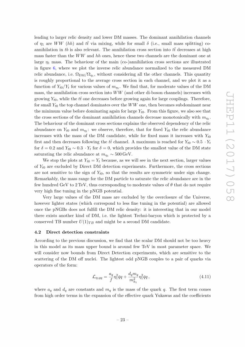
leading to larger relic density and lower DM masses. The dominant annihilation channels
of η1 are WW (hh) and tt via mixing, while for small δ (i.e., small mass splitting) co-
annihilation in tb is also relevant. The annihilation cross section into tt decreases at high
mass faster than the WW and hh ones, hence these two channels are the dominant one at
large η1 mass. The behaviour of the main (co-)annihilation cross sections are illustrated
in figure 6, where we plot the inverse relic abundance normalized to the measured DM
relic abundance, i.e. ΩDM/Ωη1 , without considering all the other channels. This quantity
is roughly proportional to the average cross section in each channel, and we plot it as a
function of Yt0/Yt for various values of mη1 . We find that, for moderate values of the DM
mass, the annihilation cross section into WW (and other di-boson channels) increases with
growing Yt0, while the tt one decreases before growing again for large couplings. Therefore,
for small Yt0 the top channel dominates over the WW one, then becomes subdominant near
the minimum value before dominating again for large Yt0. From this figure, we also see that
the cross sections of the dominant annihilation channels decrease monotonically with mη1 .
The behaviour of the dominant cross sections explains the observed dependency of the relic
abundance on Yt0 and mη1 : we observe, therefore, that for fixed Yt0 the relic abundance
increases with the mass of the DM candidate, while for fixed mass it increases with Yt0first and then decreases following the tt channel. A maximum is reached for Yt0 ∼ 0.5 · Ytfor δ = 0.2 and Yt0 ∼ 0.3 · Yt for δ = 0, which provides the smallest value of the DM state
saturating the relic abundance at mη1 ∼ 500 GeV.
We stop the plots at Yt0 = Yt because, as we will see in the next section, larger values
of Yt0 are excluded by Direct DM detection experiments. Furthermore, the cross sections
are not sensitive to the sign of Yt0, so that the results are symmetric under sign change.
Remarkably, the mass range for the DM particle to saturate the relic abundance are in the
few hundred GeV to 2 TeV, thus corresponding to moderate values of θ that do not require
very high fine tuning in the pNGB potential.
Very large values of the DM mass are excluded by the overclosure of the Universe,
however lighter states (which correspond to less fine tuning in the potential) are allowed
once the pNGBs does not fulfill the DM relic density: it is interesting that in our model
there exists another kind of DM, i.e. the lightest Techni-baryon which is protected by a
conserved TB number U(1)TB and might be a second DM candidate.
4.2 Direct detection constraints
According to the previous discussion, we find that the scalar DM should not be too heavy
in this model as its mass upper bound is around few TeV in most parameter space. We
will consider now bounds from Direct Detection experiments, which are sensitive to the
scattering of the DM off nuclei. The lightest odd pNGB couples to a pair of quarks via
operators of the form:
Lη1qq =aqfη2
1 qq +dqmq
m2h1
η21 qq , (4.11)
where aq and dq are constants and mq is the mass of the quark q. The first term comes
from high order terms in the expansion of the effective quark Yukawas and the coefficients
– 23 –

JHEP11(2017)058
aq are related to the couplings in table 3 via the mass diagonalization. The second term
is generated by exchanging the Higgs (the singlet s gives subleading corrections). In both
cases, the dominant contribution is proportional to the mass of the quark via its Yukawa
coupling. These couplings give rise to spin independent elastic cross section σSI, which may
be potentially within the reach of present and future Direct DM search experiments. Note
that, on this case, the spin-dependent cross section σSD is always much smaller than σSI,
so in the following discussion we only consider σSI. The spin-independent elastic scattering
cross section of η1 off a nucleus can be parameterised as
σSI =4
πm2η1
(mη1mn
mη1 +mn)2 [Zfp + (A− Z)fn]2
A2(4.12)
where mn is the neutron mass, Z and A − Z are the number of protons and neutrons in
the nucleus and fp (fn ) describes the coupling between η1 and protons (neutrons):
fn,p =∑
q=u,d,s
fn,pTqcqmn,p
mq+
2
27fn,pTG
∑q=c,b,t
cqmn,p
mq, (4.13)
where cq = aq/f + dqmq/m2h1
from eq. (4.11). The hadron matrix elements fn,pTqparame-
terize the quark content of the nucleons, and we take their values from [93]:
fpTu = 0.017, fpTd = 0.022, fpTs = 0.053,
fnTu = 0.011, fnTd = 0.034, fnTs = 0.053,
fp,nTG = 1−∑
q=u,d,s
fp,nTq . (4.14)
For an alternative numerical evaluation of the above parameters, we refer the reader to
refs. [94, 95].
The effective couplings in eq. (4.11) depend on Yf0 via the mass mixing terms and the
presence of off-diagonal couplings in table 3, we therefore decided to compute the elastic
cross sections for fixed values of Yf0/Yf to be compared to the relic abundance calculation
in figure 5. Since the thermal relic density of η1 is a function of its mass, to compare the
theoretical cross section to the experimental constraints we need to take into account the
difference between the local DM density and the actual density of η1: therefore, in figure 7
we rescale the inelastic cross section according to
σEXPSI =
Ωη1
ΩDMσSI , (4.15)
to compare with the experimental bounds, which assume the standard density of DM
around the Earth, ρ0 = 0.3GeV/cm3, assuming that the DM density is saturated by the
particle under consideration (and standard halo profile).
The effective cross section σEXPSI is thus compared to the current most constraining
bounds, presently coming from LUX experiment [96] on σSI: the results are shown on the
top row plots in figure 7 for δ = 0 and 0.2. We find that the region where Yf0 < 0.1Yf and
– 24 –

JHEP11(2017)058
[GeV]1
ηm500 1000 1500 2000 2500 3000
))2
/(cm
SI
σ(10
log
49−
48−
47−
46−
45−
44−
43−
42−
41−
40− t/Y
t0Y
0
0.1
0.2
0.3
0.4
0.5
0.6
0.7
0.8
0.9
1XENON-100
XENON-1T
PandaX-II
LUX-2016
LZ-projected
Thermal = 0.0δ
[GeV]1
ηm500 1000 1500 2000 2500 3000
))2
/(cm
SI
σ(10
log
49−
48−
47−
46−
45−
44−
43−
42−
41−
40− t/Y
t0Y
0
0.1
0.2
0.3
0.4
0.5
0.6
0.7
0.8
0.9
1XENON-100
XENON-1T
PandaX-II
LUX-2016
LZ-projected
Thermal = 0.2δ
[GeV]1
ηm500 1000 1500 2000 2500 3000
))2
/(cm
SI
σ(10
log
49−
48−
47−
46−
45−
44−
43−
42−
41−
40− t/Y
t0Y
0
0.1
0.2
0.3
0.4
0.5
0.6
0.7
0.8
0.9
1XENON-100
XENON-1T
PandaX-II
LUX-2016
LZ-projected
Non-thermal = 0.0δ
[GeV]1
ηm500 1000 1500 2000 2500 3000
))2
/(cm
SI
σ(10
log
49−
48−
47−
46−
45−
44−
43−
42−
41−
40− t/Y
t0Y
0
0.1
0.2
0.3
0.4
0.5
0.6
0.7
0.8
0.9
1XENON-100
XENON-1T
PandaX-II
LUX-2016
LZ-projected
Non-thermal = 0.2δ
Figure 7. Spin-independent cross section for the elastic scattering of the DM candidate η1 off
nuclei compared to current and future experimental sensitivities. The upper plots show cross
sections rescaled to the thermal relic abundance (overabundant points are not shown), while the
lower ones assume relic abundance equal to the measured one.
Yf0 > 0.8Yf are almost excluded. For intermediate values of Yf0, 0.1Yf < Yf0 < 0.8Yf ,
the upper limit on the η1 mass is around 1 TeV for both cases, δ = 0 and 0.2. The
future experiment XENON1T [97] and LZ-projected [98] can stringently limit the model
parameter space and eventually exclude most of the parameter space in case of thermally
produced DM. We remark that the right edge of the points corresponds to the parameter
space saturating the measured relic abundance. If non-thermal production mechanisms for
the DM are allowed, it may be possible that the correct relic density is obtained in the
whole parameter space: under this pragmatic assumption, we compared the cross section
with the experimental bounds in the bottom row of figure 7. In this case, the cross section
becomes nontrivially dependent on the value of Yf0 and LUX limits can exclude DM masses
below 800 GeV for Yf0 < 0.1Yf and 3000 GeV for Yf0 > 0.9Yf in the case of δ = 0. For
δ = 0.2, the lower limits on DM mass are 800 GeV and 1500 GeV for this two region of Yf0
respectively. The projected reach of future experiments will be able to extend the exclusion
to a few TeV.
4.3 Indirect detection constraints
Indirect DM detection relies on astronomical observations of fluxes of SM particles reaching
Earth to detect the products of annihilation or decay of DM in our galaxy and throughout
– 25 –

JHEP11(2017)058
the cosmos. The differential flux of DM annihilation products can be written as
Φ(ψ,E) = (σv)dNi
dE
1
4πm2DM
∫line of sight
ds ρ2(r(s, ψ)) , (4.16)
where E is the energy of the particle i (either direct product of the annihilation, or gen-
erated as a secondary particle during the diffusion in the Galaxy) and ψ is the angle from
the direction of the sky pointing to the centre of our Galaxy. The cross section (σv) is the
annihilation in a specific final state that produces the particle i as primary or secondary
product with a differential spectrum dNi/dE, while ρ is the DM profile distribution in the
Galaxy at a distance r from the centre of the Galaxy, and s is the distance from Earth run-
ning along the line of sight defined by ψ. Once the DM distribution profile in the Galaxy ρ
is determined, the flux of particle i can constrain the DM annihilation cross section. From
each annihilation channel, the expected flux for each detectable particle specie i can be
computed [99]. We will use these results to constrain our model by demanding that the
annihilation cross section of η1 does not exceed the observed value of the various fluxes.
Similarly to the case of Direct detection, the DM distribution profile ρη1 need to be
rescaled to take into account the actual thermal relic abundance where η1 only represent
part of the total DM density (assuming its profile follows the standard lore):
ρη1 =Ωη1
ΩDMρ. (4.17)
Thus, the physical annihilation cross section should have the following relation with the
experimental value according to eq. (4.16):
(σv)EXP =
(Ωη1
ΩDM
)2
(σv)η1 . (4.18)
In this model, the Sommerfeld enhancement [100] is very small because the couplings
of one Higgs/W/Z to η1 pairs are not large enough. Therefore, we will neglect this effect.
There are the following annihilation modes:
• η1 can annihilate into leptons and light quarks pairs via direct couplings: however,
under the assumption that Yf0 ∼ Yf so that the coupling to light fermions is roughly
proportional to their mass, these annihilation modes are very small and no significant
constraints emerge.
• Annihilation into bb can be larger than that into light fermions because of the
larger Yukawa coupling of the bottom quark. In the top row of figure 8 we show
the theoretical prediction (coloured region) for the rescaled velocity-averaged cross
section (σbbv)EXP for the annihilation channel bb. The solid black and red curves
are the limits based on Fermi-LAT gamma-ray observation and HESS respectively.
We found that, varying 0 ≤ Yb0 ≤ Yb, the rescaled cross section ranges between
(σbbv)EXP = 10−27 ÷ 10−29 cm3/s in the allowed DM mass range. We can see that
the limits from Fermi-LAT and HESS are about two to three orders of magnitude
– 26 –

JHEP11(2017)058
[GeV]1
ηm500 1000 1500 2000 2500 3000
))-1
s3
v>
/(cm
σ(<
10
log
30−
28−
26−
24−
22−
t/Y
t0Y
0
0.1
0.2
0.3
0.4
0.5
0.6
0.7
0.8
0.9
1
Fermi-LAT
H.E.S.S.
bb = 0.0δThermal
[GeV]1
ηm500 1000 1500 2000 2500 3000
))-1
s3
v>
/(cm
σ(<
10
log
30−
28−
26−
24−
22−
t/Y
t0Y
0
0.1
0.2
0.3
0.4
0.5
0.6
0.7
0.8
0.9
1
Fermi-LAT
H.E.S.S.
bb = 0.2δThermal
[GeV]1
ηm500 1000 1500 2000 2500 3000
))-1
s3
v>
/(cm
σ(<
10
log
30−
28−
26−
24−
22−
t/Y
t0Y
0
0.1
0.2
0.3
0.4
0.5
0.6
0.7
0.8
0.9
1
H.E.S.S.
tt = 0.0δThermal
[GeV]1
ηm500 1000 1500 2000 2500 3000
))-1
s3
v>
/(cm
σ(<
10
log
28−
27−
26−
25−
24−
23−
22−
21− t/Y
t0Y
0
0.1
0.2
0.3
0.4
0.5
0.6
0.7
0.8
0.9
1
H.E.S.S.
tt = 0.2δThermal
[GeV]1
ηm500 1000 1500 2000 2500 3000
))-1
s3
v>
/(cm
σ(<
10
log
28−
27−
26−
25−
24−
23−
22−
21− t/Y
t0Y
0
0.1
0.2
0.3
0.4
0.5
0.6
0.7
0.8
0.9
1
Fermi-LAT
H.E.S.S.
WW = 0.0δThermal
[GeV]1
ηm500 1000 1500 2000 2500 3000
))-1
s3
v>
/(cm
σ(<
10
log
28−
27−
26−
25−
24−
23−
22−
21− t/Y
t0Y
0
0.1
0.2
0.3
0.4
0.5
0.6
0.7
0.8
0.9
1
Fermi-LAT
H.E.S.S.
WW = 0.2δThermal
Figure 8. Theoretical prediction (coloured region) for the velocity-averaged cross section for η1annihilation into bottom pair (top row), top pair (middle row) and WW (bottom row) for δ = 0
(left) and 0.2 (right), compared to the upper limits from Fermi-LAT (black) and HESS (red) gamma-
ray observation. The colour code indicates the variation of the Yukawa coupling Yf0 from 0 to Yf .
The cross sections are rescaled to the thermal relic abundance.
too weak to impose any useful bounds for the whole mass region. Releasing the as-
sumption that DM is thermally produced, i.e. assuming that it is always saturating
the DM abundance, the cross section are enhanced for low masses, still remaining
below the Fermi-LAT current bound, as shown in the first row of figure 9.
• Annihilation into top pairs tt is further enhanced by the top Yukawa coupling. We
find that, in the same range as for the bottom, the rescaled cross section shown in
– 27 –
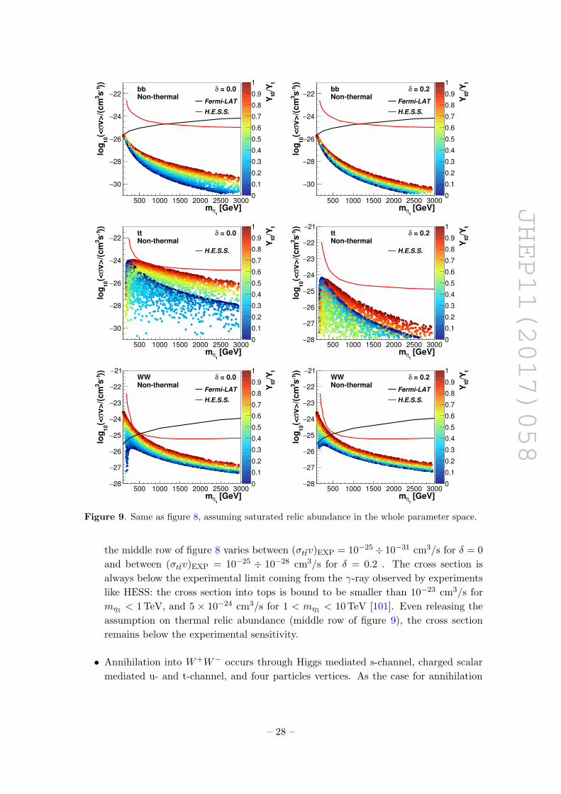
JHEP11(2017)058
[GeV]1
ηm500 1000 1500 2000 2500 3000
))-1
s3
v>
/(cm
σ(<
10
log
30−
28−
26−
24−
22−
t/Y
t0Y
0
0.1
0.2
0.3
0.4
0.5
0.6
0.7
0.8
0.9
1
Fermi-LAT
H.E.S.S.
bb = 0.0δNon-thermal
[GeV]1
ηm500 1000 1500 2000 2500 3000
))-1
s3
v>
/(cm
σ(<
10
log
30−
28−
26−
24−
22−
t/Y
t0Y
0
0.1
0.2
0.3
0.4
0.5
0.6
0.7
0.8
0.9
1
Fermi-LAT
H.E.S.S.
bb = 0.2δNon-thermal
[GeV]1
ηm500 1000 1500 2000 2500 3000
))-1
s3
v>
/(cm
σ(<
10
log
30−
28−
26−
24−
22−
t/Y
t0Y
0
0.1
0.2
0.3
0.4
0.5
0.6
0.7
0.8
0.9
1
H.E.S.S.
tt = 0.0δNon-thermal
[GeV]1
ηm500 1000 1500 2000 2500 3000
))-1
s3
v>
/(cm
σ(<
10
log
28−
27−
26−
25−
24−
23−
22−
21− t/Y
t0Y
0
0.1
0.2
0.3
0.4
0.5
0.6
0.7
0.8
0.9
1
H.E.S.S.
tt = 0.2δNon-thermal
[GeV]1
ηm500 1000 1500 2000 2500 3000
))-1
s3
v>
/(cm
σ(<
10
log
28−
27−
26−
25−
24−
23−
22−
21− t/Y
t0Y
0
0.1
0.2
0.3
0.4
0.5
0.6
0.7
0.8
0.9
1
Fermi-LAT
H.E.S.S.
WW = 0.0δNon-thermal
[GeV]1
ηm500 1000 1500 2000 2500 3000
))-1
s3
v>
/(cm
σ(<
10
log
28−
27−
26−
25−
24−
23−
22−
21− t/Y
t0Y
0
0.1
0.2
0.3
0.4
0.5
0.6
0.7
0.8
0.9
1
Fermi-LAT
H.E.S.S.
WW = 0.2δNon-thermal
Figure 9. Same as figure 8, assuming saturated relic abundance in the whole parameter space.
the middle row of figure 8 varies between (σttv)EXP = 10−25 ÷ 10−31 cm3/s for δ = 0
and between (σttv)EXP = 10−25 ÷ 10−28 cm3/s for δ = 0.2 . The cross section is
always below the experimental limit coming from the γ-ray observed by experiments
like HESS: the cross section into tops is bound to be smaller than 10−23 cm3/s for
mη1 < 1 TeV, and 5 × 10⁻²⁴ cm3/s for 1 < mη1 < 10 TeV [101]. Even releasing the
assumption on thermal relic abundance (middle row of figure 9), the cross section
remains below the experimental sensitivity.
• Annihilation into W+W− occurs through Higgs mediated s-channel, charged scalar
mediated u- and t-channel, and four particles vertices. As the case for annihilation
– 28 –

JHEP11(2017)058
Figure 10. Combination of constraints from the relic density measurement and direct detection
experiments. The region to the right of the black line is excluded by overclosure of the Universe,
while the region within the red line is still allowed by the direct detection.
into fermion pairs, in the bottom row of figure 8 we also show theoretical predic-
tions (coloured regions) for the rescaled velocity-averaged cross section (σWW v)EXP:
we see that this channel has larger cross sections than the fermionic channels and
(σWW v)EXP increases with mass. However, no bound is imposed on this channel by
Fermi-LAT nor HESS. Releasing the assumption of thermally produced relic abun-
dance (bottom row of figure 9), the cross section increases in the low mass region,
and exclusions around 500 GeV are observed, depending on the value of Yf0.
As already mentioned above, Indirect detection reach on DM models can be signifi-
cantly enhanced if large Sommerfeld enhancement factors are possible. In our model, η1 is
almost a SU(2)L singlet except for small mixing with the SU(2)L doublet and triplet, thus
it has small couplings to the EW gauge boson. We also checked the possible Sommerfeld
enhancement induced by Higgs exchange and find this effect to also be quite small: in
fact, the “Yukawa” potential V (r) = −αhr e−mhr is suppressed by θ2. In conclusion, we find
that DM indirect detection can not impose significant constraints on this model if η1 is a
thermally produced DM component.
4.4 Summary of DM constraints
Previously we separately discusses the constraints on the DM candidate η1 from different
DM experimental tests. We now combine all these constraints to extract the allowed
parameter space in order to guide future research projects. The final summary is shown
in figure 10, where we show the constraints from DM relic density and direct detection
measurements (indirect detection does not impose any stronger bounds on η1). The region
allowed by direct detection is within the red line (the grey area being excluded), while the
black line corresponds to the parameters fulfilling the thermal relic density. We recall the
reader that the region on the right of the black line is excluded by overclosure, while on
– 29 –

JHEP11(2017)058
the left η1 can only partly accommodate for the full DM density, as shown in figure 5. The
surviving region where η1 can be the unique DM candidate consists of mη1 ∈ [500, 1000] GeV
and Yt0/Yt ∈ [0.12, 0.5] for δ = 0 and mη1 ∈ [500, 800] GeV and Yt0/Yt ∈ [0.28, 0.75] for
δ = 0.2. Larger (and smaller) values of Yt0 are only allowed for small mη1 (and low
DM thermal relic density), which are however in tension with electroweak precision tests:
θ > 0.2 roughly corresponds to mη1 > 500 GeV. The DM candidate η1 still has a wide
parameter spaces to provide enough relic density.
5 Technicolor interacting massive particles as dark matter
In this section, we would like to briefly discuss the possibility that the Techni-baryons,
protected by a global TB number, may play the role of DM. This possibility was first
discussed in [57] in the context of Technicolour theories. As the Techni-baryons are strongly
interacting, it is difficult to calculate the annihilation rate: however, approximating it by
the geometrical cross section allows to estimate the value of the required masses to be,
generically, around 100 TeV. This value would point toward values of the condensation
scale of at least a few TeV, thus in a more fine tuned region of the parameter space in
terms of generating the pNGB Higgs boson.
Another intriguing possibility is that an asymmetry is generated via the electroweak
baryogenesis [102, 103], in the same way as a lepton and baryon asymmetry is generated.
This mechanism does, however, require that the TB number is violated by some anomalies
that preserve a combination of it with the SM baryon and/or lepton numbers [58]. In our
case, the strong sector being non-chiral with respect to the SM gauging, such anomaly is
absent and the electroweak sphaleron would be ineffective in balancing the asymmetries.
We are therefore left with two mechanisms to generate a Techni-baryon asymmetry:
• break U(1)TB by a gauge sphaleron process at a higher scale than the electroweak
phase transition;
• explicitly break U(1)TB.
For the former case, we need to assume that the theory is UV completed by an extended
gauge sector (in a similar fashion to Extended Technicolor models [12]) which is chiral. At
the scale where the new gauge theory is spontaneously broken (by condensation or a Higgs
mechanism), we need a strong first order phase transition and sufficient CP violation in
order to generate an asymmetry in the TB number in a similar way as baryogenesis [104].
The net asymmetry is then left unchanged at the electroweak phase transition. This
mechanism can be very attractive if the model is UV completed by a chiral theory that
gives mass to the top at a scale not far from the condensation scale [105].
In the latter case, we assume that the TB number is violated explicitly by new interac-
tions at a very high scale that couple the Techni-fermions to SM particles. Depending on
the number of FCD-colours, the low energy effect may be a linear mixing to SM fermions
(odd NFCD) or couplings to fermion bilinears (even NTC). For instance, in the case of
– 30 –

JHEP11(2017)058
NTC = 3, a 4-Fermion interaction may be induced in the form:
1
Λ2l εabcψaψbψc → λl lL , (5.1)
where L = 〈εabcψaψbψc〉 is one Techni-baryon and a, b, c stand for the FCD-colour indices.
The field l is a generic lepton (including neutrinos), so that this interaction preserves L
+ TB. The mediator generating such interaction can thus be invoked as generator of TB
asymmetry in the same way as in Grand Unification baryogenesis models [104]: at the UV
scale, out of equilibrium decays of the mediator will produce an asymmetry if CP is also
violated. However, the same operator will induce decays of the composite Techni-baryons
at low energy. This drawback can be avoided if the theory is conformal in the UV, as it
can be achieved by adding additional flavours [72]. A mass gap is only generated at the
low scale where conformality is lost, and the running of the operator will generate a large
suppression if the anomalous dimensions of the Techni-baryon operator is small [67]. In
fact, λl is related to the UV scale by
λl ∼(
ΛTC
Λ
)2−γΛTC , (5.2)
where γ is the anomalous dimension of the 〈εabcψaψbψc〉 composite operator. A very small
λl, i.e. a large Λ, can thus guarantee long lived Techni-baryons at Cosmological scales.
Assuming that the mass of the baryon is ΛTC , the mixing angle between lepton l and
Techni-baryon is sin θl = λlΛTC
for λl ΛTC . The Techni-baryon main decay channels are
L→ lW/Z through gauge interaction. By simple calculation and assuming γ ∼ 0, we find
that the UV scale should be above Λ ∼ 1013 GeV to ensure Cosmologically stable Techni-
baryons. Mixing with quarks can also be written if additional coloured Techni-fermions
are added, as in ref. [43].
Direct detection experiments typically impose very stringent bounds on a composite
fermionic DM candidate because of its magnetic moment. However, it is possible that
the lightest Techni-baryon is made of electromagnetically neutral Techni-fermions (and
potentially mixes to the right-handed neutrino) and thus has vanishing magnetic moment,
thus avoiding the constraints.
6 Conclusions
It’s tantalising to think that the Higgs boson may be a composite state of a more fun-
damental confining dynamics. In this work, we explore the possibility that, along with
the Higgs, the dynamics produces also a light scalar DM candidate, arising from the same
symmetry breaking responsible for the breaking of the EW symmetry. The minimal model
featuring this property is based on the symmetry breaking SU(4)×SU(4)/SU(4). It is also
the only consistent model where a DM pNGB can be shown to exist, also featuring a simple
underlying description in terms of a gauge-fermion theory.
The main features of the model have been described in ref. [38]: in this work we focus
on the parameter space where the DM candidate is stable, and numerically explore the
– 31 –

JHEP11(2017)058
constraints coming from thermal relic abundance and Direct/Indirect DM detection. The
neutral DM candidate is accompanied by several neutral and charged companions, whose
mass is close to the DM one. One needs, therefore, to consider co-annihilation. The main
free parameters determining the properties of the DM candidate are an additional Yukawa
coupling Yf0, which does not enter the mass of the light SM fermions, and a mass splitting
between the underlying Techni-fermions δ. We also focus on the case δ ≥ 0, where the
lightest odd states are mostly made of gauge singlets, in order to avoid strong constraints
from Direct detection experiments.
We show that, under reasonable simplifying assumptions, the thermal relic abundance
can saturate the measured value for masses of the lightest neutral pNGB between 500 GeV
to 2 TeV, depending on the value of two free parameters. Remarkably, larger values of the
masses are excluded by overabundance, thus providing an interesting upper limit on the
condensation scale and on the fine-tuning parameter sin θ. We also study the constraints
coming from Direct and Indirect detection. Under the assumption of thermally produced
DM, we find that only Direct Detection is sensitive to the available parameter space. In fact,
regions with small and large values of the Yukawa coupling Yf0 are almost excluded by the
LUX bound, while intermediate regions still survive with roughly 0.1 Yf < Yf0 < 0.8 Yf .
In this window, the largest allowed mass is about 1 TeV for both choices of the mass
splitting δ that we consider. Future projections of Direct detection experiments show that
more parameter space will be probed in the near future. On the other hand, the cross
sections for Indirect Detection always fall short of the current bounds by 1 to 2 orders of
magnitude. The fact that low mass DM candidates are preferred gives a change to the
LHC for complementary reach on this model, even though we showed via very preliminary
estimation that it is very challenging to produce and detect the additional scalar pNGBs.
We also tested the case where the DM is not thermally produced, thus matching the
relic abundance to the observed one in the whole parameter space. Direct detection, thus,
excludes large values of the Yukawa up to large masses (3 TeV for δ = 0 and 1.5 TeV for
δ = 0.2), while small values of Yf0 are probed up to smaller masses (roughly 800 GeV in
both cases). For indirect experiments, we find some sensitivity in the tt channel around
500 GeV, while the WW channel allows to exclude masses up to 600 GeV for large Yt0 (in
the range 0.3÷ 1 Yt).
This class of models also has an additional candidate in the form of Techni-baryons
made of N Techni-fermions transforming as the fundamental of the SU(N) confining group.
While the thermal relic abundance is typically too low, an asymmetry may be generated in
a similar fashion as baryogenesis in the SM, giving rise to an asymmetric DM candidate.
However, in the simplest realization of this model, the TB number is a conserved quantity,
and thus the sphaleron mechanism is not active, unless the UV physics generates additional
interactions.
Acknowledgments
We thank the France China Particle Physics Laboratory (FCPPL) for supporting this
project. T.M. is supported in part by project Y6Y2581B11 supported by 2016 National
– 32 –

JHEP11(2017)058
Postdoctoral Program for Innovative Talents. G.C. acknowledges partial support from
the Labex-LIO (Lyon Institute of Origins) under grant ANR-10-LABX-66 and FRAMA
(FR3127, Federation de Recherche “Andre Marie Ampere”).
A Interactions of the exotic pNGBs
A.1 Singlet s
Below, we will review and discuss all the possible coupling leading to decays (and single
production) for the DM-even singlet.
Gauge and Chiral Lagrangian Interactions: we first consider couplings generated by
the gauged chiral Lagrangian. As we work in a basis where we expand around the true
vacuum of the theory (which includes the misalignment), this term is fully invariant
under a shift symmetry of all the pNGBs except the Higgs candidate. This is enough
to ensure that no couplings linear in s appear.
WZW anomaly: direct couplings of s to two gauge bosons are generated by the WZW
anomaly, giving rise to the couplings
LWZW =5iCg2
4c2θW
s εµναβ(2√
2c2θW
cos θ∂βW+µ ∂νW
−α
+√
2s2θW cos θ∂βZµ∂νAα +√
2c2θW cos θ∂βZµ∂νZα) (A.1)
with C = iNTC240π2 . The two-body decay width for each channel is
Γ(s→W+µ W
−µ ) =
g4 cos2 θ(M2s − 4m2
W )32
16384π5f2;
Γ(s→ ZµZµ) =g4c2
2θWcos2 θ(M2
s − 4m2Z)
32
131072π5f2c4θW
;
Γ(s→ ZµAµ) =g4s2
θWcos2 θ
16384π5M3s c
2θWf2
(M2s −m2
Z)3 . (A.2)
Note that, like in SU(4)/Sp(4), no coupling to two photons appears [45].
Yukawa couplings: the Yukawa coupling can potentially generate linear couplings of s to
a pair of fermions, however according to eq. (2.10) such coupling is absent.8 This is
because, although the general Yukawas break the parities A and B, they are invariant
under a global SU(4) symmetry under which s is odd:
Σ→ P †ΣP , P =
(0 1
−1 0
). (A.3)
8Additional couplings may be generated depending on the representation of the composite fermions in
the partial compositeness scenario, see [62, 106] for examples.
– 33 –

JHEP11(2017)058
Under the above parity:
s→ −s H2 → −H2 ∆↔ N. (A.4)
The operator P is an element of SU(4) which exchanges the SU(2)L and SU(2)Rsubgroups of SU(4), and it is thus broken by the EW gauging. According to this
symmetry, the allowed couplings need to involve at least another pNGB:
s(∆−N) ff ′ , sH2 ff , s2 ff . (A.5)
From table 3 in appendix B.2, however, we see that only the coupling with the triplets
is generated besides the one with s2, furthermore such coupling vanishes in the DM-
preserving Yukawas (as it is proportional to YfD). Thus, we can assume that no
decay of s is generated by the Yukawa couplings.
Higher order couplings to fermions: as the symmetries forbidding the couplings of s
to two fermions are finally broken, higher order Yukawa-like operators will gener-
ate such couplings, in particular via breaking of the parity described in the above
paragraph. Such breaking is due to the gauging of the EW group, and to different
techniquark masses for the two doublets (i.e. the parameter δ). Following [36] we will
focus here on the latter as an illustration.9 The higher order operator we consider
can be written as (where we take the top as an example):
LYuk−2 = −(QαLtR) Φα + h.c. , (A.6)
with
Φ =[Tr[MTQΣP1,α(y′′t1Σ + y′′t2Σ†)] + (iσ2)αβTr[MTQΣP β2 (y′′t3Σ + y′′t4Σ†)]
]+[Tr[MTQΣ†P1,α(y′t1Σ + y′t2Σ†)] + (iσ2)αβTr[MTQΣ†P β2 (y′t3Σ + y′t4Σ†)]
],
(A.7)
where MTQ is the Techni-fermion mass matrix. Even though, in principle, 8 new
Yukawas appear in this operator, we can follow the simplifying assumptions that
they are proportional to the lowest order Yukawas up to form factors: y′′ti = a′′yti and
y′ti = a′yti. We find single s Yukawa coupling:
i(mL +mR)
f(a′′ − a′)δ Yt sin θ s tLtR + h.c. (A.8)
which is proportional to the masses of the fermions, and also to the symmetry break-
ing parameter δ. Note also the proportionality to δa = a′′ − a′ that breaks the
A-parity. To estimate the size of this effect, following [45] we compare it to the shift
in the top mass generated by the same operators in eq. (A.6):
δmt =1√2
(mL +mR) sin 2θ ((a′′ + a′)Yt + δa(Yt0 + (YtD + YtT )δ) . (A.9)
9See [45] for an example of the effect of gauge couplings plus Yukawas.
– 34 –

JHEP11(2017)058
Assuming that the combination of Yukawas appearing in eqs. (A.8) and (A.9) are of
the same order, the coupling of s can be estimated as
gstLtR ∼ i2δmt
vSMδ tan θ ∼ i 0.14 δ tan θ , (A.10)
where we have allowed for a maximum 10% correction to the top mass.
Thus, the partial decay width of the channel s→ ff is
Γ(s→ ff) =6|gsfLfR |
2
16πM2s
√(M2
s − 4m2f )(M2
s − 2m2f ). (A.11)
As s couples to quarks, so it can couple to both gluon and photon pairs by quark
loop (dominated by the top). The decay widths of these two channels are [45]:
Γ(s→ gg) =αα2
sM3s
8π2m2W s
2W
|gstLtR |2v2
m2t
F 21 (xt). (A.12)
Γ(s→ γγ) = 1/2N2c
α2
α2s
(2
3
)4
Γ(s→ gg), (A.13)
where F1(xt) is the form factor of top loop and xt =4m2
tM2s
,
F1(xt) = 1/2xt(1 + (1− xt) sin2(x−1/2t )). (A.14)
Scalar potential: decays of s to a pair of pNGBs can also be generated via the potential
that aligns the vacuum. Following the leading potential we used in this paper, the
couplings read:
Lpot ⊃Ctf√
2sin2 θYf Im(Yf0) s
(1
2(N2
0 −∆20) + (N+N− −∆+∆−)
)+Cgf
32sin θ s
(4g2 ± (g2 − g′2) cos θ)A0∆0/N0 (A.15)
+i(4g2 − 2g′2 ± (g2 + g′
2) cos θ) (H+∆−/N− −∆+/N+H−)
;
where the couplings are evaluated at the minimum of the potential. We thus see that
s can only decay into a pair of DM-odd pNGBs, however those decays will always be
kinematically unaccessible.10
A.2 DM-odd scalars
The interactions relevant for production and decays are the following, where we label by
πi a generic odd scalar.
Gauge interactions are generated by the lowest order chiral Lagrangian, and contain
couplings of the form gπ1π2V Vµπ1←→∂µπ2 (see ref. [38] for the explicit expressions). The
corresponding decay width is
Γ(π2 → π1Vµ) = |gπ1π2V |2(M2
π2 − (Mπ1 +mV )2)(M2π2 − (Mπ1 −mV )2)
32
16πm2VM
3π2
.
(A.16)10In principle it is possible to have different mass spectra, however the couplings will also be modified.
– 35 –

JHEP11(2017)058
Yukawa couplings generate interactions of two pNGBs with two fermions, as in table 3,
thus decays of the form π2 → π1ff are generated. However, this process has usually
very small rates, so we will not consider it further.
The scalar potential generates couplings between 3 pNGBs, thus giving rise to decays
π2 → π1φ, with φ = s, h1. This partial decay width is
Γ(π2 → π1φ) =|gπ2π1φ|2
16πM3π2
√λ(M2
π2 ,M2π1 ,M
2φ) (A.17)
with λ(x, y, z) = x2 + y2 + z2 − 2xy − 2yz − 2xz. The couplings with the singlet
s are in eq. (A.15): within our choice of potential, the masses of the 3 pNGBs will
always make the decay kinematically inaccessible. On the other hand, decays with
the lighter Higgs boson h1 are allowed: keeping only the terms proportional to the
top Yukawas, the couplings can be written as
Lpot ⊃Ctf
2√
2Y 2f sin(2θ)h1
(1
2(h2
2 +A20 + ∆2
0 +N20 ) +H+H− + ∆+∆− +N+N−
)+Ctf
2Yf h1 (Re(Yf0) cos θ h2 + Im(Yf0) cos(2θ) A0) (∆0 +N0)
+Ctf
2Yf h1
(Re(Yf0) cos θ H+(N− −∆−)
+iIm(Yf0) cos(2θ) H+(N− + ∆−))
+ h.c., (A.18)
plusing additional corrections from the gauge interactions.
B Relevant couplings
In this section we list all the couplings of the pNGBs, relevant for the calculation of the
relic abundance, and other properties of the DM candidate.
B.1 Potential
Trilinear couplings. Defining:
RY = Re[Yu · Yu0]− Re[Yd · Yd0]− Re[Ye · Ye0] , (B.1)
IY = Im[Yu · Yu0] + Im[Yd · Yd0] + Im[Ye · Ye0] . (B.2)
Ltri =m2h
2vSMcos θ
(h3
1 + h1s2)
+ gsππ sπiπj + ghππ h1πiπj , (B.3)
gsN0N0 = −gs∆0∆0 =Ctf
2√
2sin2 θ IY , (B.4)
gsN+N− = −gs∆+∆− =Ctf√
2sin2 θ IY , (B.5)
gsA0N0/∆0=
Cg
16√
2
4m2W ∓ (2m2
W −m2Z) cos θ
vSM, (B.6)
– 36 –

JHEP11(2017)058
gsH+N−/∆− = g∗sH−N+/∆+ = iCg
16√
2
6m2W − 2m2
Z ∓m2Z cos θ
vSM. (B.7)
ghh2h2 =m2h
2vSMcos θ , (B.8)
ghA0A0 =cos θ
2vSM
(m2h +
Cg8
(2m2W −m2
Z)
), (B.9)
ghH+H− =cos θ
vSM
(m2h +
Cg8m2Z
), (B.10)
ghN0N0/∆0∆0=
cos θ
2vSM
(m2h −
Cg16
(2m2W −m2
Z)± Cg4
m2W
cos θ
), (B.11)
ghN0∆0 = − Cg16vSM
(2m2W −m2
Z) cos θ , (B.12)
ghN+N−/∆+∆− =cos θ
vSM
(m2h −
Cg16m2Z ±
Cg8
3m2W −m2
Z
cos θ
), (B.13)
ghN+∆− = gh∆+N− = − cos θ
16vSMCgm
2Z , (B.14)
ghh2N0 = ghh2∆0 =Ctf
2cos θ RY , (B.15)
ghA0N0 = ghA0∆0 =Ctf
2cos 2θ IY , (B.16)
ghH+N−/∆− = g∗hH−N+/∆+ =Ctf
2(± cos θ RY + i cos 2θ IY ) . (B.17)
Quartic couplings.
Lqua =m2h
24v2SM
((3− 7 sin2 θ)h4
1 + 2(1− 5 sin2 θ)h21s
2 − (1 + 3 sin2 θ)s4)
+gssππs2πiπj + gshππshπiπj + ghhππh
2πiπj + gπππππiπjπlπk .
(B.18)
gssh2h2 = − 1
12v2SM
(m2h(1 + 3 sin2 θ) +
Cg8
(2m2W +m2
Z
), (B.19)
gssA0A0 = − 1
12v2SM
(m2h(1 + 3 sin2 θ) +
Cg8
(2(1 + sin2 θ)m2W + cos2 θm2
Z
),(B.20)
gssN0N0/∆0∆0= −
m2h
4v2SM
(1 + sin2 θ ∓ δ cos θ) , (B.21)
gssN0∆0 =Cg
16v2SM
sin2 θ(2m2W −m2
Z) , (B.22)
gssh2N0/∆0= − Ct
6√
2sin θ RY , (B.23)
gssA0N0/∆0= − Ct
6√
2sin θ cos θ IY , (B.24)
gssH+H− = − 1
6v2SM
(m2h(1 + 3 sin2 θ) +
Cg8
(2m2
W +m2Z(1 + sin2 θ)
)), (B.25)
– 37 –

JHEP11(2017)058
gssN+N−/∆+∆− = −m2h
2v2SM
(1 + sin2 θ ∓ δ cos θ) . (B.26)
gssN+∆− = gssN−∆+ =Cg
16v2SM
sin2 θm2z , (B.27)
gssH+N−/∆− = g∗ssH−N+/∆+ = − Ct
6√
2sin θ(±RY + i cos θ IY ) . (B.28)
gshA0N0/∆0= ± 1
6√
2v2SM
(m2h(sin2 θ ∓ δ cos θ)
− Cg16
(2m2
W (3− 4 sin2 θ ∓ 4 cos θ)−m2Z(1− 4 sin2 θ)
)), (B.29)
gshN0N0 = −gsh∆0∆0 =Ct6
sin θ cos θ IY . (B.30)
gshH+N−/∆− = g∗shH−N+/∆+ = ± i
3√
2
(m2h(sin2 θ ∓ δ cos θ)
− Cg16
(m2W 2(1∓ 6 cos θ) +m2
Z(3− 4 sin2 θ ± 4 cos θ)))
, (B.31)
gshN+N−/∆+∆− = ±Ct6
sin 2θ IY . (B.32)
ghhh2h2 =1
12v2SM
(m2h(1− 5 sin2 θ)− Cg
8(2m2
W +m2Z)
)(B.33)
ghhA0A0 =1
4v2SM
(m2h(1− 3 sin2 θ) +
Cg8
cos(2θ)(2m2W −m2
Z)
)(B.34)
ghhN0N0/∆0∆0=
1
12v2SM
(m2h(2− 7 sin2 θ ± 2δ cos θ)
− Cg16
(m2W 2(5− 6 sin2 θ ∓ 8 cos θ)−m2
Z3(1− 2 sin2 θ)))
, (B.35)
ghhN0∆0 =1
6v2SM
(m2h(cos 2θ)− Cg
16
(m2W 2(1− 6 sin2 θ)−m2
Z3(cos 2θ)))
, (B.36)
ghhA0N0/∆0= − Ct
4√
2sin 2θ IY , (B.37)
ghhh2N0/∆0= − Ct
6√
2sin θ RY . (B.38)
ghhH+H− =1
2v2SM
(m2h(1− 3 sin2 θ) +
Cg8m2Z cos 2θ
), (B.39)
ghhN+N−/∆+∆− =1
6v2SM
(m2h(2− 7 sin2 θ ± δ cos θ)
− Cg16
(m2W 2(1∓ 12 cos θ) +m2
Z(5− 6 sin2 θ ± 8 cos θ)))
, (B.40)
ghhH+N−/∆− = g∗hhH−N+/∆+ = − Ct
6√
2sin θ (±RY + 3i cos θ IY ) . (B.41)
– 38 –

JHEP11(2017)058
B.2 Yukawa couplings
The couplings of two pNGBs to fermions, defined in eq. (2.17), are listed in the following
table 3.
ξNu , ξNd,e h1 h2 A0 ∆0 N0 s
h1 Yf sin θ 0 ±YfD sin θ ∓iYfT√2
cos θ ∓iYfT√2
cos θ 0
h2 0 Yf sin θ 0 ±Yf0√2
±Yf0√2
0
A0 ±YfD sin θ 0 Yf sin θ −iYf0√2
cos θ −iYf0√2
cos θ 0
∆ ∓iYfT√2
cos θ ±Yf0√2
−iYf0√2
cos θ Yf sin θ 0 ±YfD√2
sin θ
N ∓iYfT√2
cos θ ±Yf0√2
−iYf0√2
cos θ 0 Yf sin θ ∓YfD√2
sin θ
s 0 0 0 ±YfD√2
sin θ ∓YfD√2
sin θ Yf sin θ
ξ+u , ξ
−d,e H∓ ∆∓ N∓
h1 ∓i√
2YfD sin θ −iYfT cos θ −iYfT cos θ
h2 0 Yf0 Yf0
A0 0 ∓iYf0 ±iYf0
∆ Yf0 0 0
N −Yf0 0 0
s 0 YfD sin θ −YfD sin θ
ξCu , ξCd,e H− ∆− N−
H+ Yf sin θ ∓Yf0(1∓cos θ)√
2±Yf0
(1±cos θ)√2
∆+ ∓Yf0(1±cos θ)√
2Yf sin θ 0
N+ ±Yf0(1∓cos θ)√
20 Yf sin θ
Table 3. Couplings of two pNGBs to fermions generated by the effective Yukawas. The first table
lists the couplings of two neutral pNGBs; the second one lists the couplings of one charged and one
neutral pNGB; and the third one lists the couplings of two charged pNGBs (the signs refer to up
and down/leptons, respectively).
Open Access. This article is distributed under the terms of the Creative Commons
Attribution License (CC-BY 4.0), which permits any use, distribution and reproduction in
any medium, provided the original author(s) and source are credited.
References
[1] ATLAS collaboration, Observation of a new particle in the search for the standard model
Higgs boson with the ATLAS detector at the LHC, Phys. Lett. B 716 (2012) 1
[arXiv:1207.7214] [INSPIRE].
– 39 –

JHEP11(2017)058
[2] CMS collaboration, Observation of a new boson at a mass of 125 GeV with the CMS
experiment at the LHC, Phys. Lett. B 716 (2012) 30 [arXiv:1207.7235] [INSPIRE].
[3] N. Arkani-Hamed et al., The minimal moose for a little Higgs, JHEP 08 (2002) 021
[hep-ph/0206020] [INSPIRE].
[4] M. Schmaltz, Physics beyond the standard model (theory): introducing the little Higgs, Nucl.
Phys. Proc. Suppl. 117 (2003) 40 [hep-ph/0210415] [INSPIRE].
[5] Z. Chacko, H.-S. Goh and R. Harnik, The twin Higgs: natural electroweak breaking from
mirror symmetry, Phys. Rev. Lett. 96 (2006) 231802 [hep-ph/0506256] [INSPIRE].
[6] C. Csaki, T. Ma and J. Shu, Maximally symmetric composite Higgs models, Phys. Rev. Lett.
119 (2017) 131803 [arXiv:1702.00405] [INSPIRE].
[7] N.S. Manton, A new six-dimensional approach to the Weinberg-Salam model, Nucl. Phys. B
158 (1979) 141 [INSPIRE].
[8] D.B. Fairlie, Higgs’ fields and the determination of the Weinberg angle, Phys. Lett. 82B
(1979) 97 [INSPIRE].
[9] Y. Hosotani, Dynamical mass generation by compact extra dimensions, Phys. Lett. 126B
(1983) 309 [INSPIRE].
[10] S. Weinberg, Implications of dynamical symmetry breaking, Phys. Rev. D 13 (1976) 974
[INSPIRE].
[11] L. Susskind, Dynamics of spontaneous symmetry breaking in the Weinberg-Salam theory,
Phys. Rev. D 20 (1979) 2619 [INSPIRE].
[12] S. Dimopoulos and L. Susskind, Mass without scalars, Nucl. Phys. B 155 (1979) 237
[INSPIRE].
[13] E. Eichten and K.D. Lane, Dynamical breaking of weak interaction symmetries, Phys. Lett.
90B (1980) 125 [INSPIRE].
[14] E. Farhi and L. Susskind, Technicolour, Phys. Rep. 74 (1980) 277.
[15] M.E. Peskin and T. Takeuchi, A new constraint on a strongly interacting Higgs sector,
Phys. Rev. Lett. 65 (1990) 964 [INSPIRE].
[16] D.B. Kaplan and H. Georgi, SU(2) ×U(1) breaking by vacuum misalignment, Phys. Lett. B
136 (1984) 183 [INSPIRE].
[17] D.B. Kaplan, H. Georgi and S. Dimopoulos, Composite Higgs scalars, Phys. Lett. 136B
(1984) 187 [INSPIRE].
[18] H. Georgi and D.B. Kaplan, Composite Higgs and custodial SU(2), Phys. Lett. 145B (1984)
216 [INSPIRE].
[19] B. Holdom, Raising the sideways scale, Phys. Rev. D 24 (1981) 1441 [INSPIRE].
[20] K. Yamawaki, M. Bando and K.-i. Matumoto, Scale invariant technicolor model and a
technidilaton, Phys. Rev. Lett. 56 (1986) 1335 [INSPIRE].
[21] M. Bando, K.-i. Matumoto and K. Yamawaki, Technidilaton, Phys. Lett. B 178 (1986) 308
[INSPIRE].
[22] D.D. Dietrich, F. Sannino and K. Tuominen, Light composite Higgs from higher
representations versus electroweak precision measurements: Predictions for CERN LHC,
Phys. Rev. D 72 (2005) 055001 [hep-ph/0505059] [INSPIRE].
[23] T. Appelquist and Y. Bai, A light dilaton in walking gauge theories, Phys. Rev. D 82
(2010) 071701 [arXiv:1006.4375] [INSPIRE].
– 40 –

JHEP11(2017)058
[24] D. Elander and M. Piai, Light scalars from a compact fifth dimension, JHEP 01 (2011) 026
[arXiv:1010.1964] [INSPIRE].
[25] R. Foadi, M.T. Frandsen and F. Sannino, 125 GeV Higgs boson from a not so light
technicolor scalar, Phys. Rev. D 87 (2013) 095001 [arXiv:1211.1083] [INSPIRE].
[26] Z. Fodor, K. Holland, J. Kuti, D. Nogradi, C. Schroeder and C.H. Wong, Can the nearly
conformal sextet gauge model hide the Higgs impostor?, Phys. Lett. B 718 (2012) 657
[arXiv:1209.0391] [INSPIRE].
[27] Z. Fodor, K. Holland, J. Kuti, S. Mondal, D. Nogradi and C.H. Wong, Toward the minimal
realization of a light composite Higgs, PoS(LATTICE 2014)244 [arXiv:1502.00028]
[INSPIRE].
[28] B. Holdom and J. Terning, A light dilaton in gauge theories?, Phys. Lett. B 187 (1987) 357
[INSPIRE].
[29] B. Holdom and J. Terning, No light dilaton in gauge theories, Phys. Lett. B 200 (1988) 338
[INSPIRE].
[30] J.M. Maldacena, The large-N limit of superconformal field theories and supergravity, Int. J.
Theor. Phys. 38 (1999) 1113 [hep-th/9711200] [INSPIRE].
[31] L. Randall and R. Sundrum, An alternative to compactification, Phys. Rev. Lett. 83 (1999)
4690 [hep-th/9906064] [INSPIRE].
[32] K. Agashe, R. Contino and A. Pomarol, The minimal composite Higgs model, Nucl. Phys.
B 719 (2005) 165 [hep-ph/0412089] [INSPIRE].
[33] D.B. Kaplan, Flavor at SSC energies: a new mechanism for dynamically generated fermion
masses, Nucl. Phys. B 365 (1991) 259 [INSPIRE].
[34] R. Contino and A. Pomarol, Holography for fermions, JHEP 11 (2004) 058
[hep-th/0406257] [INSPIRE].
[35] G. Cacciapaglia, G. Marandella and J. Terning, Dimensions of supersymmetric operators
from AdS/CFT, JHEP 06 (2009) 027 [arXiv:0802.2946] [INSPIRE].
[36] J. Galloway, J.A. Evans, M.A. Luty and R.A. Tacchi, Minimal conformal technicolor and
precision electroweak tests, JHEP 10 (2010) 086 [arXiv:1001.1361] [INSPIRE].
[37] G. Cacciapaglia and F. Sannino, Fundamental composite (goldstone) Higgs dynamics, JHEP
04 (2014) 111 [arXiv:1402.0233] [INSPIRE].
[38] T. Ma and G. Cacciapaglia, Fundamental composite 2HDM: SU(N) with 4 flavours, JHEP
03 (2016) 211 [arXiv:1508.07014] [INSPIRE].
[39] J. Barnard, T. Gherghetta and T.S. Ray, UV descriptions of composite Higgs models
without elementary scalars, JHEP 02 (2014) 002 [arXiv:1311.6562] [INSPIRE].
[40] G. Ferretti and D. Karateev, Fermionic UV completions of composite Higgs models, JHEP
03 (2014) 077 [arXiv:1312.5330] [INSPIRE].
[41] G. Ferretti, UV completions of partial compositeness: the case for a SU(4) gauge group,
JHEP 06 (2014) 142 [arXiv:1404.7137] [INSPIRE].
[42] G. von Gersdorff, E. Ponton and R. Rosenfeld, The dynamical composite Higgs, JHEP 06
(2015) 119 [arXiv:1502.07340] [INSPIRE].
[43] L. Vecchi, A dangerous irrelevant UV-completion of the composite Higgs, JHEP 02 (2017)
094 [arXiv:1506.00623] [INSPIRE].
– 41 –

JHEP11(2017)058
[44] T.A. Ryttov and F. Sannino, Ultra minimal technicolor and its dark matter TIMP, Phys.
Rev. D 78 (2008) 115010 [arXiv:0809.0713] [INSPIRE].
[45] A. Arbey et al., Fundamental composite electroweak dynamics: status at the LHC, Phys.
Rev. D 95 (2017) 015028 [arXiv:1502.04718] [INSPIRE].
[46] M. Frigerio, A. Pomarol, F. Riva and A. Urbano, Composite scalar dark matter, JHEP 07
(2012) 015 [arXiv:1204.2808] [INSPIRE].
[47] D. Marzocca and A. Urbano, Composite dark matter and LHC interplay, JHEP 07 (2014)
107 [arXiv:1404.7419] [INSPIRE].
[48] J. Wess and B. Zumino, Consequences of anomalous Ward identities, Phys. Lett. 37B
(1971) 95 [INSPIRE].
[49] E. Witten, Current algebra, baryons and quark confinement, Nucl. Phys. B 223 (1983) 433
[INSPIRE].
[50] Z.-y. Duan, P.S. Rodrigues da Silva and F. Sannino, Enhanced global symmetry constraints
on epsilon terms, Nucl. Phys. B 592 (2001) 371 [hep-ph/0001303] [INSPIRE].
[51] O. Antipin, M. Redi, A. Strumia and E. Vigiani, Accidental composite dark matter, JHEP
07 (2015) 039 [arXiv:1503.08749] [INSPIRE].
[52] A. Carmona and M. Chala, Composite dark sectors, JHEP 06 (2015) 105
[arXiv:1504.00332] [INSPIRE].
[53] S.I. Blinnikov and M. Khlopov, Possible astronomical effects of mirror particles, Sov.
Astron. 27 (1983) 371 [INSPIRE].
[54] R.N. Mohapatra, S. Nussinov and V.L. Teplitz, Mirror matter as selfinteracting dark
matter, Phys. Rev. D 66 (2002) 063002 [hep-ph/0111381] [INSPIRE].
[55] R. Foot, Mirror matter-type dark matter, Int. J. Mod. Phys. D 13 (2004) 2161
[astro-ph/0407623] [INSPIRE].
[56] D.E. Kaplan, G.Z. Krnjaic, K.R. Rehermann and C.M. Wells, Atomic dark matter, JCAP
05 (2010) 021 [arXiv:0909.0753] [INSPIRE].
[57] S. Nussinov, Technocosmology: could a technibaryon excess provide a ‘natural’ missing mass
candidate?, Phys. Lett. 165B (1985) 55 [INSPIRE].
[58] S.M. Barr, R.S. Chivukula and E. Farhi, Electroweak fermion number violation and the
production of stable particles in the early universe, Phys. Lett. B 241 (1990) 387 [INSPIRE].
[59] S. Nussinov, Some estimates of interaction in matter of neutral technibaryons made of
colored constituents, Phys. Lett. B 279 (1992) 111 [INSPIRE].
[60] B. Bellazzini, C. Csaki and J. Serra, Composite Higgses, Eur. Phys. J. C 74 (2014) 2766
[arXiv:1401.2457] [INSPIRE].
[61] J. Mrazek et al., The other natural two Higgs doublet model, Nucl. Phys. B 853 (2011) 1
[arXiv:1105.5403] [INSPIRE].
[62] B. Gripaios, A. Pomarol, F. Riva and J. Serra, Beyond the Minimal Composite Higgs
Model, JHEP 04 (2009) 070 [arXiv:0902.1483] [INSPIRE].
[63] D. Marzocca, M. Serone and J. Shu, General composite Higgs models, JHEP 08 (2012) 013
[arXiv:1205.0770] [INSPIRE].
[64] R. Contino and M. Salvarezza, One-loop effects from spin-1 resonances in Composite Higgs
models, JHEP 07 (2015) 065 [arXiv:1504.02750] [INSPIRE].
– 42 –

JHEP11(2017)058
[65] D. Ghosh, M. Salvarezza and F. Senia, Extending the analysis of electroweak precision
constraints in composite Higgs models, Nucl. Phys. B 914 (2017) 346 [arXiv:1511.08235]
[INSPIRE].
[66] R.C. Brower, A. Hasenfratz, C. Rebbi, E. Weinberg and O. Witzel, Composite Higgs model
at a conformal fixed point, Phys. Rev. D 93 (2016) 075028 [arXiv:1512.02576] [INSPIRE].
[67] C. Pica and F. Sannino, Anomalous dimensions of conformal baryons, Phys. Rev. D 94
(2016) 071702 [arXiv:1604.02572] [INSPIRE].
[68] T. Appelquist, G.T. Fleming and E.T. Neil, Lattice study of conformal behavior in SU(3)
Yang-Mills theories, Phys. Rev. D 79 (2009) 076010 [arXiv:0901.3766] [INSPIRE].
[69] Y. Aoki et al., Lattice study of conformality in twelve-flavor QCD, Phys. Rev. D 86 (2012)
054506 [arXiv:1207.3060] [INSPIRE].
[70] A. Cheng, A. Hasenfratz, Y. Liu, G. Petropoulos and D. Schaich, Improving the continuum
limit of gradient flow step scaling, JHEP 05 (2014) 137 [arXiv:1404.0984] [INSPIRE].
[71] Z. Fodor et al., Twelve massless flavors and three colors below the conformal window, Phys.
Lett. B 703 (2011) 348 [arXiv:1104.3124] [INSPIRE].
[72] M.P. Lombardo, K. Miura, T.J. Nunes da Silva and E. Pallante, On the particle spectrum
and the conformal window, JHEP 12 (2014) 183 [arXiv:1410.0298] [INSPIRE].
[73] G. Cacciapaglia, H. Cai, T. Flacke, S.J. Lee, A. Parolini and H. Serodio, Anarchic Yukawas
and top partial compositeness: the flavour of a successful marriage, JHEP 06 (2015) 085
[arXiv:1501.03818] [INSPIRE].
[74] O. Matsedonskyi, On flavour and naturalness of composite Higgs models, JHEP 02 (2015)
154 [arXiv:1411.4638] [INSPIRE].
[75] G. Panico and A. Pomarol, Flavor hierarchies from dynamical scales, JHEP 07 (2016) 097
[arXiv:1603.06609] [INSPIRE].
[76] F. Sannino, A. Strumia, A. Tesi and E. Vigiani, Fundamental partial compositeness, JHEP
11 (2016) 029 [arXiv:1607.01659] [INSPIRE].
[77] R. Arthur, V. Drach, M. Hansen, A. Hietanen, C. Pica and F. Sannino, SU(2) gauge theory
with two fundamental flavors: a minimal template for model building, Phys. Rev. D 94
(2016) 094507 [arXiv:1602.06559] [INSPIRE].
[78] J. Rantaharju, V. Drach, A. Hietanen, C. Pica and F. Sannino, Wilson fermions with four
fermion interactions, PoS(LATTICE 2015)228 [arXiv:1511.03899] [INSPIRE].
[79] R. Foadi, Effect of four-fermion operators on the mass of the composite particles,
arXiv:1601.02676 [INSPIRE].
[80] Quark Flavor Physics Working Group collaboration, J.N. Butler et al., Working
Group Report: Quark Flavor Physics, in the proceedings of the Community Summer Study
2013: Snowmass on the Mississippi (CSS2013), July 29–August 6, Minneapolis, U.S.A.
(2013), arXiv:1311.1076 [INSPIRE].
[81] ATLAS collaboration, Search for new phenomena in final states with an energetic jet and
large missing transverse momentum in pp collisions at√s = 8 TeV with the ATLAS
detector, Eur. Phys. J. C 75 (2015) 299 [arXiv:1502.01518] [INSPIRE].
[82] CMS collaboration, Search for dark matter, extra dimensions and unparticles in monojet
events in proton-proton collisions at√s = 8 TeV, Eur. Phys. J. C 75 (2015) 235
[arXiv:1408.3583] [INSPIRE].
– 43 –
JHEP11(2017)058
[83] ATLAS collaboration, Search for dark matter in events with a hadronically decaying W or
Z boson and missing transverse momentum in pp collisions at√s = 8 TeV with the ATLAS
detector, Phys. Rev. Lett. 112 (2014) 041802 [arXiv:1309.4017] [INSPIRE].
[84] CMS collaboration, Search for dark matter in proton-proton collisions at 8 TeV with
missing transverse momentum and vector boson tagged jets, JHEP 12 (2016) 083 [Erratum
ibid. 08 (2017) 035] [arXiv:1607.05764] [INSPIRE].
[85] ATLAS collaboration, Search for dark matter in events with missing transverse momentum
and a Higgs boson decaying to two photons in pp collisions at√s = 8 TeV with the ATLAS
detector, Phys. Rev. Lett. 115 (2015) 131801 [arXiv:1506.01081] [INSPIRE].
[86] ATLAS collaboration, Search for dark matter produced in association with a Higgs boson
decaying to two bottom quarks in pp collisions at√s = 8 TeV with the ATLAS detector,
Phys. Rev. D 93 (2016) 072007 [arXiv:1510.06218] [INSPIRE].
[87] ATLAS collaboration, Search for dark matter in association with a Higgs boson decaying to
b-quarks in pp collisions at√s = 13 TeV with the ATLAS detector, Phys. Lett. B 765
(2017) 11 [arXiv:1609.04572] [INSPIRE].
[88] S. Wolfram, Abundances of stable particles produced in the early universe, Phys. Lett. 82B
(1979) 65 [INSPIRE].
[89] K. Griest and D. Seckel, Three exceptions in the calculation of relic abundances, Phys. Rev.
D 43 (1991) 3191 [INSPIRE].
[90] E.W. Kolb and M.S. Turner, The early universe, Front. Phys. 69 (1990) 1 [INSPIRE].
[91] P. Gondolo and G. Gelmini, Cosmic abundances of stable particles: Improved analysis,
Nucl. Phys. B 360 (1991) 145 [INSPIRE].
[92] Planck collaboration, P.A.R. Ade et al., Planck 2015 results. XIII. Cosmological
parameters, Astron. Astrophys. 594 (2016) A13 [arXiv:1502.01589] [INSPIRE].
[93] H.-Y. Cheng and C.-W. Chiang, Revisiting scalar and pseudoscalar couplings with nucleons,
JHEP 07 (2012) 009 [arXiv:1202.1292] [INSPIRE].
[94] J.M. Alarcon, J. Martin Camalich and J.A. Oller, The chiral representation of the πN
scattering amplitude and the pion-nucleon sigma term, Phys. Rev. D 85 (2012) 051503
[arXiv:1110.3797] [INSPIRE].
[95] J.M. Alarcon, L.S. Geng, J. Martin Camalich and J.A. Oller, The strangeness content of the
nucleon from effective field theory and phenomenology, Phys. Lett. B 730 (2014) 342
[arXiv:1209.2870] [INSPIRE].
[96] LUX collaboration, D.S. Akerib et al., Results from a search for dark matter in the
complete LUX exposure, Phys. Rev. Lett. 118 (2017) 021303 [arXiv:1608.07648] [INSPIRE].
[97] XENON collaboration, E. Aprile et al., Physics reach of the XENON1T dark matter
experiment, JCAP 04 (2016) 027 [arXiv:1512.07501] [INSPIRE].
[98] LZ collaboration, D.S. Akerib et al., Lux-Zeplin (LZ) conceptual design report,
arXiv:1509.02910 [INSPIRE].
[99] M. Cirelli et al., PPPC 4 DM ID: a poor particle physicist cookbook for dark matter indirect
detection, JCAP 03 (2011) 051 [Erratum ibid. 10 (2012) E01] [arXiv:1012.4515]
[INSPIRE].
[100] J.L. Feng, M. Kaplinghat and H.-B. Yu, Sommerfeld enhancements for thermal relic dark
matter, Phys. Rev. D 82 (2010) 083525 [arXiv:1005.4678] [INSPIRE].
– 44 –
JHEP11(2017)058
[101] H.E.S.S. collaboration, H. Abdallah et al., Search for dark matter annihilations towards
the inner Galactic halo from 10 years of observations with H.E.S.S, Phys. Rev. Lett. 117
(2016) 111301 [arXiv:1607.08142] [INSPIRE].
[102] K. Petraki and R.R. Volkas, Review of asymmetric dark matter, Int. J. Mod. Phys. A 28
(2013) 1330028 [arXiv:1305.4939] [INSPIRE].
[103] K.M. Zurek, Asymmetric dark matter: theories, signatures and constraints, Phys. Rept. 537
(2014) 91 [arXiv:1308.0338] [INSPIRE].
[104] A.D. Sakharov, Violation of CP invariance, c asymmetry and baryon asymmetry of the
universe, Pisma Zh. Eksp. Teor. Fiz. 5 (1967) 32 [INSPIRE].
[105] G. Cacciapaglia and F. Sannino, An ultraviolet chiral theory of the top for the fundamental
composite (Goldstone) Higgs, Phys. Lett. B 755 (2016) 328 [arXiv:1508.00016] [INSPIRE].
[106] J. Serra, Beyond the minimal top partner decay, JHEP 09 (2015) 176 [arXiv:1506.05110]
[INSPIRE].
– 45 –