Pulse Code Modulation (PCM)

◮ PCM in the Bell System

◮ Multiplexing PCM

◮ Asynchronous PCM

◮ Extensions to PCM

◮ Differential PCM (DPCM)

◮ Adaptive DPCM (ADPCM)

◮ Delta-Sigma Modulation (DM)

◮ Vocoders

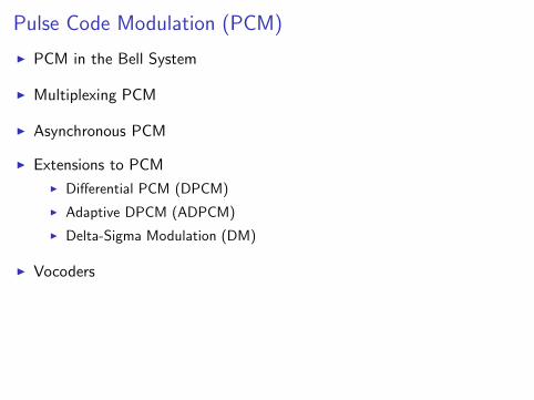
PCM in the Bell System

Starting in the 1920s, long distance telephone links used frequency divisionmultiplexing. (FDM requires amplifiers, built using vacuum tubes.)

A cable with bandwidth 3 MHz can support (in principle) 1000 3 kHz voicechannels. But 1000 filters, modulators, and demodulators are needed.

Local exchanges communicated by trunk lines. Each copper pair carried onevoice conversation.

Using PCM, multiple connections could be time division multiplexed.

The Bell System settled on 1.544 Mbit/s (by experimentation).

8000 · (24 · 8 + 1) = 8000 · 193 = 1544000

This TDM signal is called digital signal level 1 (DS1).

This T-1 carrier system uses the same copper that was used for voice!

PCM is credited to Bernard Oliver and Claude Shannon (patent 2,801,281, 1946)

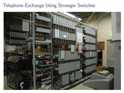
Telephone Exchange Using Strowger Switches

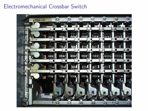
Electromechanical Crossbar Switch

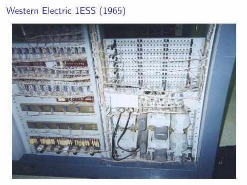
Western Electric 1ESS (1965)

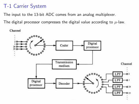
T-1 Carrier System

The input to the 13-bit ADC comes from an analog multiplexer.

The digital processor compresses the digital value according to µ-law.

T-1 Carrier System (cont.)

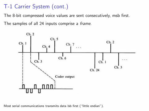
The 8-bit compressed voice values are sent consecutively, msb first.

The samples of all 24 inputs comprise a frame.

Most serial communications transmits data lsb first (“little endian”).

T-1 Frame

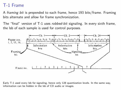
A framing bit is prepended to each frame, hence 193 bits/frame. Framingbits alternate and allow for frame synchronization.

The “final” version of T-1 uses robbed-bit signaling. In every sixth frame,the lsb of each sample is used for control purposes.

Early T-1 used every lsb for signaling, hence only 128 quantization levels. In the same way,information can be hidden in the lsb of CD audio or images.

T-Carrier (T-CXR)

T-1 links can be multiplexed over high-speed links (wire, microwave,optical). Multiplexing is by bits, not octets.

T-2: 4 T-1 channels (96 voice), 6.312 Mbs (copper)

T-3: 7 T-2 channels (672 voice), 44.736 Mbs (copper)

T-4: 6 T-3 channels (4032 voice), 274.176 Mbs

Customers could buy a T-1 link or part of a link (fractional T-1).

A common digital link in the 1990s was 56000 bps. This was one T-1channel with 7 bits/sample at 8 kHz.

The European hierarchy is similar but was designed after T-carrier.

E1 has 32 8-bit channels but uses two for frame synchronization andsignaling.

E1–E5 have 32, 128, 512, 2048, 8192 channels. The channels are not

combined by bitwise multiplexing.

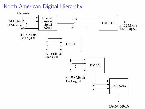
North American Digital Hierarchy

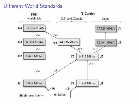
Different World Standards

Multiplexing PCM

A major motivation for PCM is the ability to multiplex many low bit ratechannels on a single hit bit rate channel. There are many ways to do this:

◮ Bit interleaving

◮ Word interleaving

These each have advantages and disadvantages. A major issue issynchronization. There are several different approaches

◮ Synchronous: hard to do in practice

◮ Asynchronous: potentially wasteful of capacity

◮ Plesiochronous: a practical balance

Greek “plesos” meaning almost. (The plesiosaur is not a dinosaur but a large swimming reptile.)

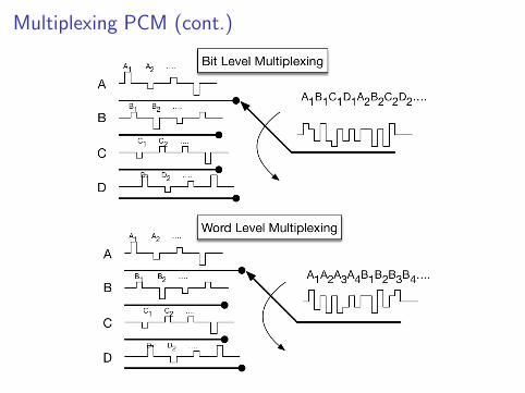
Multiplexing PCM (cont.)

Asynchronous PCM

It is difficult to ensure that bits arrive and leave at synchronous rates.

Example:

◮ 100 km cable carrying 200 Mbits/s.

◮ If temperature increases by 1◦F, propagation velocity increases by 0.01%.

◮ This results in a temporary increase of 20 kbits/s in the bit arrival rate.

What do we do with all the extra bits?

Answers:

◮ Run the link at a slightly slower bit rate, and bit stuff the extra bitsempty bits if we don’t need them.

◮ Run the link at a slightly lower bit rate, and drop occasional LSBs.

◮ Run at the ideal rate, and bit stuff/bit delete as needed.

We use the control channel to indicate which bits are stuffed/deleted.

Differential PCM

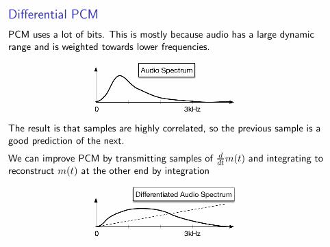
PCM uses a lot of bits. This is mostly because audio has a large dynamicrange and is weighted towards lower frequencies.

The result is that samples are highly correlated, so the previous sample is agood prediction of the next.

We can improve PCM by transmitting samples of d

dtm(t) and integrating to

reconstruct m(t) at the other end by integration

Differential PCM (cont.)

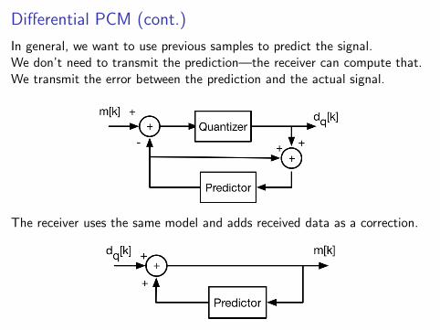
In general, we want to use previous samples to predict the signal.We don’t need to transmit the prediction—the receiver can compute that.We transmit the error between the prediction and the actual signal.

The receiver uses the same model and adds received data as a correction.

Differential PCM (cont.)

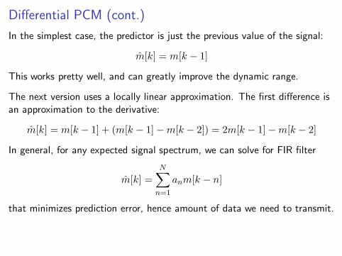
In the simplest case, the predictor is just the previous value of the signal:

m̂[k] = m[k − 1]

This works pretty well, and can greatly improve the dynamic range.

The next version uses a locally linear approximation. The first difference isan approximation to the derivative:

m̂[k] = m[k − 1] + (m[k − 1]−m[k − 2]) = 2m[k − 1]−m[k − 2]

In general, for any expected signal spectrum, we can solve for FIR filter

m̂[k] =

N∑

n=1

anm[k − n]

that minimizes prediction error, hence amount of data we need to transmit.

Adaptive Differential PCM (ADPCM)

◮ The DPCM signal will be much lower amplitude if it is a good model

◮ The number of quantization levels L is fixed

◮ ADPCM adaptively adjusts the channel gain, so that the quantizationlevels best represent the signal.

The combination of DPCM and ADPCM can reduce the number of bitsrequired by a factor of two,

This can be used to reduce the bandwidth required by a factor of two, orimprove the SNR for a fixed bandwidth.

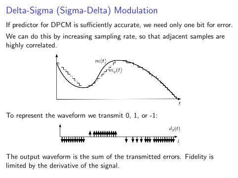
Delta-Sigma (Sigma-Delta) Modulation

If predictor for DPCM is sufficiently accurate, we need only one bit for error.

We can do this by increasing sampling rate, so that adjacent samples arehighly correlated.

To represent the waveform we transmit 0, 1, or -1:

The output waveform is the sum of the transmitted errors. Fidelity islimited by the derivative of the signal.

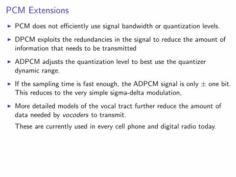
PCM Extensions

◮ PCM does not efficiently use signal bandwidth or quantization levels.

◮ DPCM exploits the redundancies in the signal to reduce the amount ofinformation that needs to be transmitted

◮ ADPCM adjusts the quantization level to best use the quantizerdynamic range.

◮ If the sampling time is fast enough, the ADPCM signal is only ± one bit.This reduces to the very simple sigma-delta modulation,

◮ More detailed models of the vocal tract further reduce the amount ofdata needed by vocoders to transmit.

These are currently used in every cell phone and digital radio today.