1

Pumps as turbines (PATs): Series and parallelconnections

Margarida Isabel Carvalho Pagaimo, ist181809

Abstract—As a result, from the high energy consumption ofthe water supply sector, several improvements have arisen for thesake of minimizing this consumption and maximizing the energyefficiency. The use of the pump operating as a turbine (PAT)is one example. It has demonstrated to be a viable solution forenergy recovery and pressure control in water systems, especiallyin remote areas where there is no access to the electrical grid.This is accomplished by means of a generator, whose operationin this specific application has been overlooked. Therefore, thisdissertation is intended to bridge this gap between the hydraulicand electric system when using PATs. This was achieved throughthe assessment of the electrical stability of the association ofmultiple PATs connected to self excited induction generators(SEIG) in water distribution systems.

In order to accomplish this, a dynamic model of a SEIG wasdeveloped. Subsequently, a model of a PAT was modelled fromits characteristic curves. Both models were validated after theirimplementation and together they formed a generating system.When two generating systems were connected in series, it wasperceived how an electrical variation in one generating systemhighly affected the subsequent system where the perturbance wasnot imposed. However, it is important to note that this conclusionapplies only for this specific PAT and SEIG. If this applicationwould be evaluated in a high-power system, the implicationsobserved in the PAT where no variation was imposed wouldmost likely turn out to be insignificant.

I. INTRODUCTION

Water supply systems have a significant environmental andenergetic impact due to the large amount of energy consumed.According to the Internation Energy Agency [3], the energyconsumption of the water sector worldwide in the form ofelectricity corresponded to 4% of the total global electricityconsumption in 2014. Of this part of electricity consumed forwater, around 40% was estimated to be used to extract water,25% for wastewater treatment and 20% for water distribution.As a result from the large energy consumption in the entirewater sector, society has become aware that improving themanagement of these systems is a crucial step towards amore sustainable and economical use of water resources. Inparticular, solutions to minimize energy consumption and tomaximize the energy efficiency have to be implemented.

The application of a pump operating as a turbine (PAT) hasbeen proven in Ramos and Borga [4] to be an alternative andsustainable solution for a better management of these watersystems. This solution has drawn a lot of attention since itcombines water saving with power generation. In detail, thePAT is able to recover energy where it is available in excess,instead of allowing its dissipation, and when coupled to agenerator this energy can be converted into electrical energy.Therefore, this is a reliable solution in the case of rural and

remote areas, where the absence of the electrical grid couldbe compensated with power generation by means of a PATand a generator, in locations with natural or artificial fallsof water. Even though the efficiency of a PAT is usuallylower than that of conventional turbines, using PATs has stilldemonstrated to be a favourable alternative to the use ofturbines for energy recovery systems. A primary advantage isthe potential cost savings. As pumps are mass produced andthere are less manufacturers of turbines, considering the use ofa pump operating as a turbine shows to be less expensive thanobtaining a specifically designed hydraulic turbine. In addition,pumps are available in a wide range of heads and flows andin a large number of standard sizes. Also, spare parts (suchas seals and bearings) are easily available, allowing for easiermaintenance.

To complement the on going advancement regarding the useof PATs, this dissertation was proposed. Its aim is to assessthe reliability of associating multiple groups of PATs, eachconnected to a generator, in order to increase the amount ofenergy recovered. This purpose demonstrates to be pertinentgiven that it is more cost-effective to invest in several lowpower pumps rather than in a single high power pump.Depending on the hydraulic system, the connections betweenthe PATs can be made in parallel or in series. Pumps connectedin parallel are suitable for a hydraulic system characterizedby high flows, as in the case of sewage treatment. On theother hand, pumps connected in series are appropriate for ahydraulic system characterized by a high head, for example inwaterfalls. Furthermore, the associations of PATs could proveto be advantageous if acting in one group of PAT coupled to agenerator does not affect the other groups significantly. If thisis proven, a fault occurring in one group does not compromisethe others groups such that they are still able to supply theirrespective low-power consumers. The evaluation of this effectconsists of the goal of this thesis. Only by assessing thisinteraction between generating groups can a conclusion bedrawn regarding the reliability of these associations.

In order to achieve this goal, a model of the SEIG and amodel of the PAT had to be implemented. This developmentand the results from the final assessment of the association ofPATs are presented here.

II. SELF EXCITED INDUCTION GENERATOR - A REVIEW

Not only Capelo [1], but also Williams et al. [5] haveidentified the squirrel cage induction generator as the mostappropriate electrical machine to take into account for energyrecovery in WDS. Simplicity, robustness, reliability and lowcost are the main reasons pointed out for this choice.

2

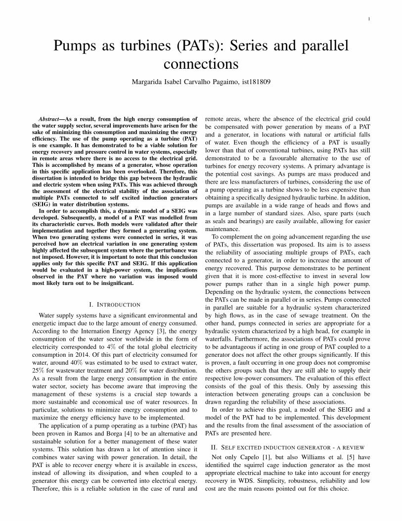
For the induction machine to run as a generator, a source ofreactive power is required. In case the machine is connectedto the grid it can draw excitation current from it. But, in thecase where the machine is operating isolated from the grid, analternative source has to be considered. For this it is commonto use capacitors as, when connected to the stator terminals,they provide the magnetizing current necessary to establishthe air-gap magnetic field. As this dissertation directs to theuse of PATs for energy recovery in remote areas, the gridcan not be taken for granted, so the main focus here will bethe stand alone operation. Figure 2 demonstrates the completegenerating system from which the SEIG is a part of. The powerflow represented in this figure can be interpreted. As the primemover transfers mechanical power Pmec to the shaft, the rotorbegins to rotate. Then, due to residual magnetism, voltage willbe induced at the stator terminals. If the capacitors are properlysized, they will provide the induction machine with the reactivepower required for voltage to build up, Qs. As excitation isachieved, if the prime mover is delivering enough Pmec to theshaft, the machines decelerate and the SEIG will supply theload with active power Ps and, in case of an inductive load,with reactive power QL.

Fig. 1: Complete power generating system.

From figure 1, it is perceived that in order to model theSEIG, the capacitor bank, the load and the prime mover haveto be modelled as well. The electrical connection between theSEIG, the capacitor bank and the load is established by:

iabcC = iabcS + iabcLvabcS = 1

C

∫(−iabcS − iabcL)dt

iabcL = 1L

∫(vabcS −RLiabcL)dt

(1)

The mechanical coupling between the SEIG and the primemover is defined by equation 2:

Jdωmdt

= Tmec − TL − Tlosses (2)

where· ωm mechanical rotor angular speed· J moment of inertia· Tmec mechanical torque developed by the prime mover· TL load torque generated by the SEIG· Tlosses torque due to friction and windage losses

From this equation it is noted that, as the prime moverand the SEIG are mechanically coupled, a state equilibrium

exists when the torque developed by the prime mover equalsthe torque requested by the mechanical load, which is thegenerator, plus the losses. In this research the prime moverstarts as a DC motor to validate the model of the SEIG and,afterwards, it is changed to the PAT.

Bearing this in mind, the model of the SEIG is developednext.

III. DYNAMIC MODEL OF THE SEIG

The dynamics of the induction machine is characterisedby differential equations with time-varying inductances dueto the continuous change in the position of the rotor withrespect to stator. This implies that when calculations are takenplace in the usual abc reference frame, being this a stationarycoordinate system, a large set of complex equations have tobe derived needing a greater effort to accomplish the dynamicanalysis. In order to lower this complexity a change to a rotat-ing reference frame is considered, accomplished by the direct-quadrature-zero (dq0) transformation. To be more precise, inthe case of balanced three-phase circuits, the application of thedq0 transformation reduces the three AC quantities to two DCquantities. As a result, the time dependency on these three-phase quantities is eliminated and the analysis becomes muchsimpler.

To start with, the three-phase stator and rotor voltageequations are as follows:

vabcs = Rsiabcs +dΨabcs

dt(3)

vabcr = 0 = RriabcR +dΨabcR

dt(4)

where the voltages (vabcR)T = [vaR vbR vcR ] are zerosince the rotor windings have their terminals short-circuitedand Rs and Rr are diagonal matrices, each with equal nonzeroelements. These three-phase voltages can be transformed intotwo-phase voltages by considering the direct and quadratureaxes in a rotating reference frame. In fact, any direct andquadrature variable can be obtained using the Park’s trans-formation, Pγ , as follows:

fdq0 = Pγfabc (5)

where

fdq0 =

fdfqf0

(6)

with fd being the direct component, fq the quadrature compo-nent and f0 the zero component. Here (fabc)

T = [fa fb fc]can represent any variable such as voltage, current or flux. Asfor the Park’s matrix, it is defined by:

Pγ =2

3

cos γ cos (γ − 120o) cos (γ + 120o)sin γ sin (γ − 120o) sin (γ + 120o)

12

12

12

(7)

where γ can either be the phase difference bewteen the d-axisand the stator phase a-axis or the angle between the d-axisand the rotor phase a-axis, depending on the variable we referto. For this reference frame it is admitted that the q-axis lags

3

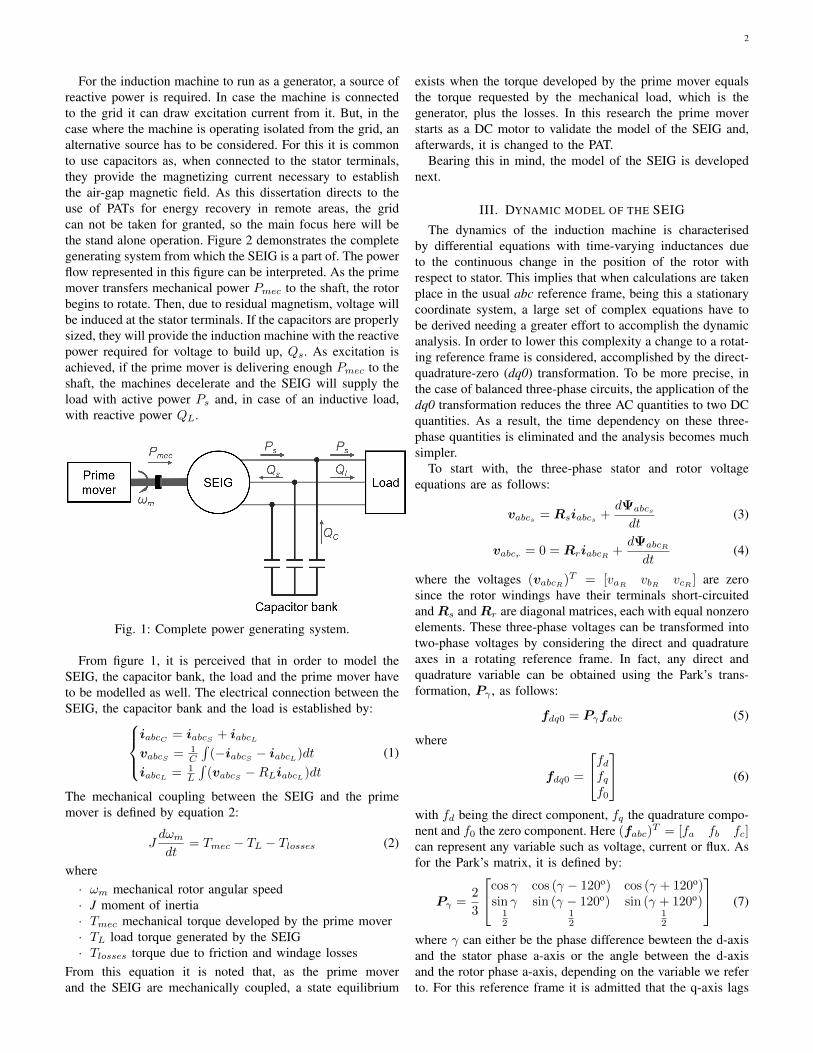
the d-axis by 90o as it can be visualized next in figure 2 andsuggested by analysing matrix 7.f0 (eq. 5) is used to make the d-q model suitable for

unbalanced three-phase systems and also to allow performingthe inverse of Park’s transformation. Under balanced three-phase conditions this component is null. Therefore, it will notbe considered any longer.

Fig. 2: Synchronously rotating d-q reference frame overlappedonto the three phase reference frame of an induction machine.

At this point, it will be assumed that the d-q reference frameis rotating at synchronous angular speed, ωs. Therefore whenseen from the stator’s perspective, the d-q axis is seen to berotating at synchronous angular speed ωs. This implies thatthe angular displacement of the d-axis with respect to thestator geometry position will be θ=ωs t at any instant. Thisis confirmed in figure 2 as the angle between the phase-a axisof the stator and the d-axis is θ. Under these circumstances,when computing the phase voltages referred to the stator, theangle γ in Park’s matrix should be replaced by θ such that:

Vabcs = P−1θ Vdq0s (8)

At the same time when seen from the rotor’s perspective thed-q reference frame is seen to be rotating at an angular speedof ωs-ωr, since the rotor itself moves at a speed of ωr. So atany moment the angular position of the d-q axis with respectto the rotor will be β = (ωs − ωr)t. Again this is verified inthe figure since this β is the angle between the axis of rotorphase-a and the d-axis. Being so, in order to establish thephase voltages related to the rotor γ should now be replacedby β as in the following equation 9:

Vabcr = P−1β Vdq0R (9)

When replacing equations 8 and 9 into equations 3 and 4,the direct and quadrature components of the stator and rotor

are defined by:

vds = Rsids +d

dtΨds +

dθ

dtΨqs (10)

vqs = Rsiqs +d

dtΨqs −

dθ

dtΨds (11)

vdr = 0 = Rridr +d

dtΨdr +

dβ

dtΨqr (12)

vqr = 0 = Rriqr +d

dtΨqr −

dβ

dtΨdr (13)

By inspecting equations 10 to 13 it can be perceived that thesystem is simplified if either θ or β are assumed to be zero.For this reason, the d-q reference frame has been chosen tobe stationary. In detail, as the d-q axis stopped rotating, theangle displacement θ is 0, such that the d-axis is aligned withthe stator phase-a axis. Following this consideration, the directand quadrature components of the flux linkages of the statorand the rotor are obtained from equations 10 to 13 as:

Ψds =

∫(vds −Rsids)dt (14)

Ψqs =

∫(vqs −Rsiqs)dt (15)

Ψdr =

∫(0−Rridr − ωrΨqr)dt (16)

Ψqr =

∫(0−Rriqr − ωrΨdr)dt (17)

Furthermore, the d-q components of the flux linkages ofthe stator and the rotor can also be determined from the d-qcomponents of the current of the stator and rotor:

Ψds = Lsids + Lmidr (18)

Ψqs = Lsiqs + Lmiqr (19)

Ψdr = Lridr + Lmids (20)

Ψqr = Lriqr + Lmiqs (21)

with Ls = λs + Lm and Lr = λr + Lm. Here λs and λr arethe stator and rotor self inductances, respectively, and Lm isthe magnetizing inductance. Taking into account equations 18to 21, the direct and quadrature currents of the stator and therotor are computed as follows:

ids =Ψds − Lmidr

Ls(22)

iqs =Ψqs − Lmiqr

Ls(23)

idr =Ψdr − Lmids

Lr(24)

iqr =Ψqr − Lmiqs

Lr(25)

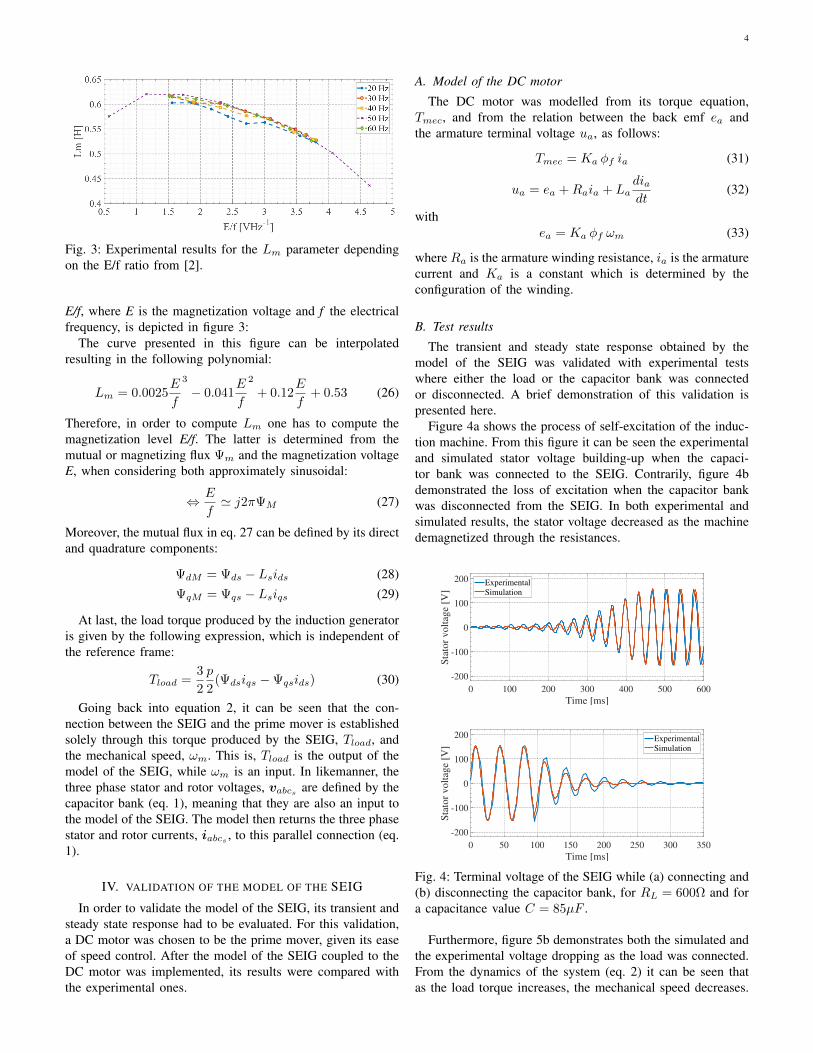
Regarding the magnetizing inductance, Lm, in [2] it wasverified that the model of the SEIG was more accurate whenthe influence of the magnetization level, E/f, in this parameterwas accounted for, with the remainder of the electrical param-eters fixed. This variation of Lm with the magnetization level

4

Fig. 3: Experimental results for the Lm parameter dependingon the E/f ratio from [2].

E/f, where E is the magnetization voltage and f the electricalfrequency, is depicted in figure 3:

The curve presented in this figure can be interpolatedresulting in the following polynomial:

Lm = 0.0025E

f

3

− 0.041E

f

2

+ 0.12E

f+ 0.53 (26)

Therefore, in order to compute Lm one has to compute themagnetization level E/f. The latter is determined from themutual or magnetizing flux Ψm and the magnetization voltageE, when considering both approximately sinusoidal:

⇔ E

f' j2πΨM (27)

Moreover, the mutual flux in eq. 27 can be defined by its directand quadrature components:

ΨdM = Ψds − Lsids (28)ΨqM = Ψqs − Lsiqs (29)

At last, the load torque produced by the induction generatoris given by the following expression, which is independent ofthe reference frame:

Tload =3

2

p

2(Ψdsiqs −Ψqsids) (30)

Going back into equation 2, it can be seen that the con-nection between the SEIG and the prime mover is establishedsolely through this torque produced by the SEIG, Tload, andthe mechanical speed, ωm. This is, Tload is the output of themodel of the SEIG, while ωm is an input. In likemanner, thethree phase stator and rotor voltages, vabcs are defined by thecapacitor bank (eq. 1), meaning that they are also an input tothe model of the SEIG. The model then returns the three phasestator and rotor currents, iabcs , to this parallel connection (eq.1).

IV. VALIDATION OF THE MODEL OF THE SEIG

In order to validate the model of the SEIG, its transient andsteady state response had to be evaluated. For this validation,a DC motor was chosen to be the prime mover, given its easeof speed control. After the model of the SEIG coupled to theDC motor was implemented, its results were compared withthe experimental ones.

A. Model of the DC motor

The DC motor was modelled from its torque equation,Tmec, and from the relation between the back emf ea andthe armature terminal voltage ua, as follows:

Tmec = Ka φf ia (31)

ua = ea +Raia + Ladiadt

(32)

withea = Ka φf ωm (33)

where Ra is the armature winding resistance, ia is the armaturecurrent and Ka is a constant which is determined by theconfiguration of the winding.

B. Test results

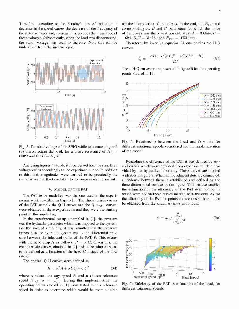
The transient and steady state response obtained by themodel of the SEIG was validated with experimental testswhere either the load or the capacitor bank was connectedor disconnected. A brief demonstration of this validation ispresented here.

Figure 4a shows the process of self-excitation of the induc-tion machine. From this figure it can be seen the experimentaland simulated stator voltage building-up when the capaci-tor bank was connected to the SEIG. Contrarily, figure 4bdemonstrated the loss of excitation when the capacitor bankwas disconnected from the SEIG. In both experimental andsimulated results, the stator voltage decreased as the machinedemagnetized through the resistances.

0 100 200 300 400 500 600

Time [ms]

-200

-100

0

100

200

Sta

tor

volt

age

[V]

Experimental

Simulation

0 50 100 150 200 250 300 350

Time [ms]

-200

-100

0

100

200

Sta

tor

volt

age

[V]

Experimental

Simulation

Fig. 4: Terminal voltage of the SEIG while (a) connecting and(b) disconnecting the capacitor bank, for RL = 600Ω and fora capacitance value C = 85µF .

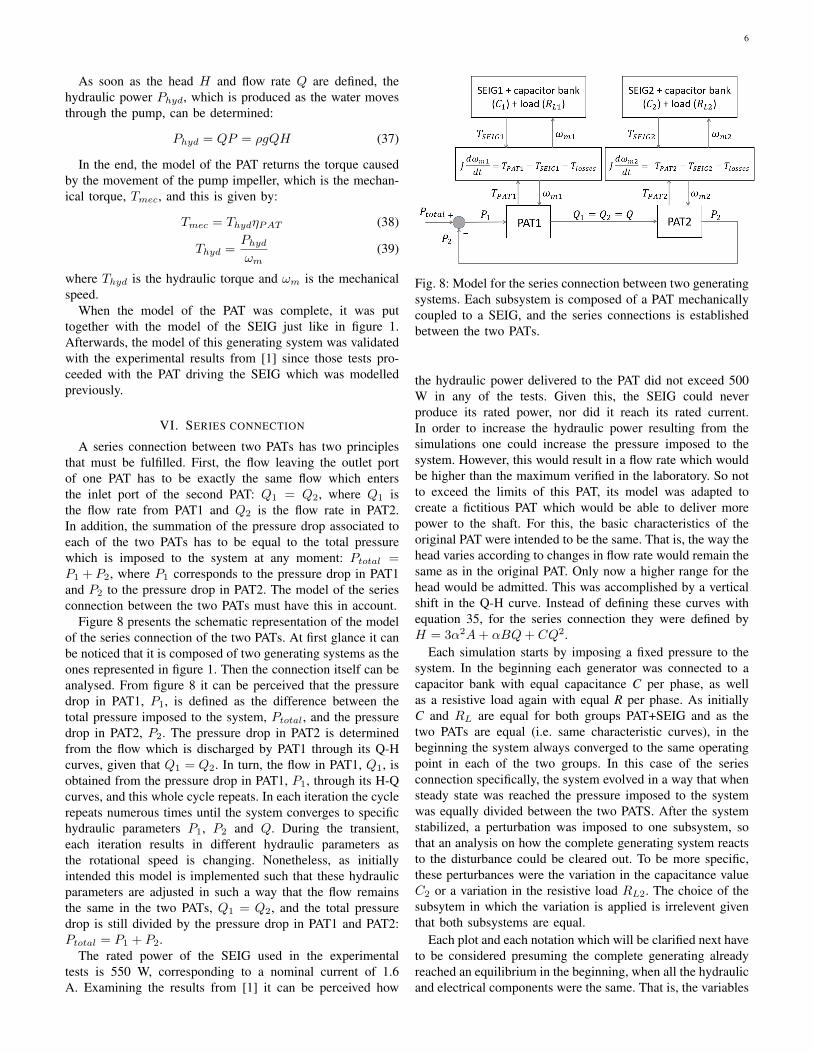
Furthermore, figure 5b demonstrates both the simulated andthe experimental voltage dropping as the load was connected.From the dynamics of the system (eq. 2) it can be seen thatas the load torque increases, the mechanical speed decreases.

5

Therefore, according to the Faraday’s law of induction, adecrease in the speed causes the decrease of the frequency ofthe stator voltages and, consequently, so does the magnitude ofthese voltages. Subsequently, when the load was disconnected,the stator voltage was seen to increase. Now this can beunderstood from the inverse logic.

0 0.5 1 1.5

Time [s]

-200

0

200

Sta

tor

Volt

age

[V]

Experimental

Simulation

0 0.2 0.4 0.6 0.8 1 1.2

Time [s]

-200

0

200

Sta

tor

Volt

age

[V]

Experimental

Simulation

Fig. 5: Terminal voltage of the SEIG while (a) connecting and(b) disconnecting the load, for a phase resistance of RL =600Ω and for C = 35µF .

Analysing figures 4a to 5b, it is perceived how the simulatedvoltage varies accordingly to the experimental one. In additionto this, their magnitudes were verified to be practically thesame, as well as the time taken to converge in each transient.

V. MODEL OF THE PAT

The PAT to be modelled was the one used in the experi-mental work described in Capelo [1]. The characteristic curvesof the PAT, namely the Q-H curves and the Q-ηPAT curves,were obtained in these experiments and they were the startingpoint to this modelling.

In the experimental set-up assembled in [1], the pressurewas the hydraulic parameter which was imposed to the system.For the sake of simplicity, it was admitted that the pressureimposed to the hydraulic system equals the differential pres-sure between the inlet and outlet of the PAT, P. This relateswith the head drop H as follows: P = ρgH . Given this, thecharacteristic curves obtained in [1] had to be adapted so asto be defined as a function of the head H instead of the flowrate Q.

The original Q-H curves were defined as:

H = α2A+ αBQ+ CQ2 (34)

where α relates the any speed N and a chosen referencespeed Nref : α = N

Nref. During this implementation, the

operating points studied in [1] were tested as this referencespeed in order to determine which would be more suitable

for the interpolation of the curves. In the end, the Nref andcorresponding A, B and C parameters for which the modeof the errors was the lowest possible was: A = 3.6644, B =−694.45, C = 314560 and Nref = 1050 rpm.

Therefore, by inverting equation 34 one obtains the H-Qcurves:

Q =−αB ±

√(αB)2 − 4C(α2A−H)

2C(35)

These H-Q curves are represented in figure 6 for the operatingpoints studied in [1].

0 5 10 15

Head [mwc]

2

3

4

5

6

7

8

Flo

w r

ate

[l/s

] N = 1525 rpm

N = 1370 rpm

N = 1200 rpm

N = 1130 rpm

N = 1050 rpm

N = 930 rpm

N = 810 rpm

Fig. 6: Relationship between the head and flow rate fordifferent rotational speeds considered for the implementationof the model.

Regarding the efficiency of the PAT, it was defined by sev-eral curves which were obtained from experimental data pro-vided by the hydraulics laboratory. These curves are markedwith dots in figure 7. When all the adjacent dots are connected,a tendency between them is established and defined by thethree-dimensional surface in the figure. This surface enablesthe estimation of the efficiency of the PAT even for pointswhich were not on these curves marked with the dots. As forthe efficiency of the PAT for points outside this surface, it canbe obtained from the similarity laws as follows:

ηi = ηref

Hi

Href

( Ni

Nref)2

(36)

10

20

0

30

40

PA

T e

ffic

iency

[%

] 50

500 15

Rotational speed [rpm]101000

Head [mwc]501500

15

20

25

30

35

40

Fig. 7: Efficiency of the PAT as a function of the head, fordifferent rotational speeds.

6

As soon as the head H and flow rate Q are defined, thehydraulic power Phyd, which is produced as the water movesthrough the pump, can be determined:

Phyd = QP = ρgQH (37)

In the end, the model of the PAT returns the torque causedby the movement of the pump impeller, which is the mechan-ical torque, Tmec, and this is given by:

Tmec = ThydηPAT (38)

Thyd =Phydωm

(39)

where Thyd is the hydraulic torque and ωm is the mechanicalspeed.

When the model of the PAT was complete, it was puttogether with the model of the SEIG just like in figure 1.Afterwards, the model of this generating system was validatedwith the experimental results from [1] since those tests pro-ceeded with the PAT driving the SEIG which was modelledpreviously.

VI. SERIES CONNECTION

A series connection between two PATs has two principlesthat must be fulfilled. First, the flow leaving the outlet portof one PAT has to be exactly the same flow which entersthe inlet port of the second PAT: Q1 = Q2, where Q1 isthe flow rate from PAT1 and Q2 is the flow rate in PAT2.In addition, the summation of the pressure drop associated toeach of the two PATs has to be equal to the total pressurewhich is imposed to the system at any moment: Ptotal =P1 + P2, where P1 corresponds to the pressure drop in PAT1and P2 to the pressure drop in PAT2. The model of the seriesconnection between the two PATs must have this in account.

Figure 8 presents the schematic representation of the modelof the series connection of the two PATs. At first glance it canbe noticed that it is composed of two generating systems as theones represented in figure 1. Then the connection itself can beanalysed. From figure 8 it can be perceived that the pressuredrop in PAT1, P1, is defined as the difference between thetotal pressure imposed to the system, Ptotal, and the pressuredrop in PAT2, P2. The pressure drop in PAT2 is determinedfrom the flow which is discharged by PAT1 through its Q-Hcurves, given that Q1 = Q2. In turn, the flow in PAT1, Q1, isobtained from the pressure drop in PAT1, P1, through its H-Qcurves, and this whole cycle repeats. In each iteration the cyclerepeats numerous times until the system converges to specifichydraulic parameters P1, P2 and Q. During the transient,each iteration results in different hydraulic parameters asthe rotational speed is changing. Nonetheless, as initiallyintended this model is implemented such that these hydraulicparameters are adjusted in such a way that the flow remainsthe same in the two PATs, Q1 = Q2, and the total pressuredrop is still divided by the pressure drop in PAT1 and PAT2:Ptotal = P1 + P2.

The rated power of the SEIG used in the experimentaltests is 550 W, corresponding to a nominal current of 1.6A. Examining the results from [1] it can be perceived how

Fig. 8: Model for the series connection between two generatingsystems. Each subsystem is composed of a PAT mechanicallycoupled to a SEIG, and the series connections is establishedbetween the two PATs.

the hydraulic power delivered to the PAT did not exceed 500W in any of the tests. Given this, the SEIG could neverproduce its rated power, nor did it reach its rated current.In order to increase the hydraulic power resulting from thesimulations one could increase the pressure imposed to thesystem. However, this would result in a flow rate which wouldbe higher than the maximum verified in the laboratory. So notto exceed the limits of this PAT, its model was adapted tocreate a fictitious PAT which would be able to deliver morepower to the shaft. For this, the basic characteristics of theoriginal PAT were intended to be the same. That is, the way thehead varies according to changes in flow rate would remain thesame as in the original PAT. Only now a higher range for thehead would be admitted. This was accomplished by a verticalshift in the Q-H curve. Instead of defining these curves withequation 35, for the series connection they were defined byH = 3α2A+ αBQ+ CQ2.

Each simulation starts by imposing a fixed pressure to thesystem. In the beginning each generator was connected to acapacitor bank with equal capacitance C per phase, as wellas a resistive load again with equal R per phase. As initiallyC and RL are equal for both groups PAT+SEIG and as thetwo PATs are equal (i.e. same characteristic curves), in thebeginning the system always converged to the same operatingpoint in each of the two groups. In this case of the seriesconnection specifically, the system evolved in a way that whensteady state was reached the pressure imposed to the systemwas equally divided between the two PATS. After the systemstabilized, a perturbation was imposed to one subsystem, sothat an analysis on how the complete generating system reactsto the disturbance could be cleared out. To be more specific,these perturbances were the variation in the capacitance valueC2 or a variation in the resistive load RL2. The choice of thesubsytem in which the variation is applied is irrelevent giventhat both subsystems are equal.

Each plot and each notation which will be clarified next haveto be considered presuming the complete generating alreadyreached an equilibrium in the beginning, when all the hydraulicand electrical components were the same. That is, the variables

7

resultant from the simulated tests are to be shown over time butonly for a specific timespan, only during the transient when theparameters C or RL were changed. The first part regarding thetransient in which the SEIG excites and the two PATs convergeto the same flow rate is not shown here.

The analysis of the test results is divided into two cathe-gories: one is the effect of increasing C or RL and the secondis the effect of decreasing C or RL. The results are grouped inthis way since, as demonstrated in the dissertation, increasingC2 or RL2 has a similar effect on the other subsystem,PAT1+SEIG1, and the same applies for decreasing C2 orRL2. In this current work, only one case from each groupis presented.

For simplicity, the subscripts A and B were adopted duringthe following explanation to refer to the operating point beforeand after the transient respectively.

A. Decreasing RLIn order to demonstrate the consequences that decreasing

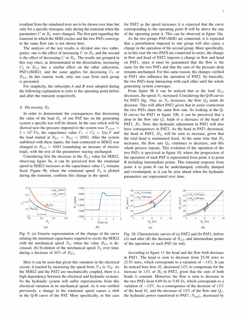
the value of the load RL of one PAT has on the generatingsystem a specific test will be shown. In the case which will beshowed next the pressure imposed to the system was Ptotal =5 × 105 Pa, the capacitance value C1 = C2 = 23µF andthe load started at RL1 = RL2 = 200Ω. After the systemstabilized with these inputs, the load connected to SEIG2 waschanged to RL2 = 160Ω (simulating an increase of electricload), with the rest of the parameters staying unchanged.

Considering first the decrease in the RL2 value for SEIG2,observing figure 9a, it can be perceived how the rotationalspeed in SEIG2 increases as the capacitance value C2 remainsfixed. Figure 9b, where the rotational speed N2 is plottedduring the transient, confirms this change in the speed.

N1 N2 N3 N4

N2

0

C1

C2

C3

C4

C2

(NB,C

B)

(NA,C

A)

RL2

=200

RL2

=160

(a)

0 1 2 3 4 5

Time [s]

1200

1300

1400

1500

1600

1700

N2 [

rpm

]

(b)

Fig. 9: (a) Generic representation of the change of the curverelating the minimum capacitance required to excite the SEIG2with the mechanical speed N2, when the value RL2 is de-creased. (b) Evolution of the mechanical speed N2 over time,during a decrease of 20% of RL2.

Here it can be seen that given this variation in the electricalcircuit, it reacted by increasing the speed from NA to NB . Asthe SEIG2 and the PAT2 are mechanically coupled, there is ahigh dependency between the electrical and hydraulic systems.So the hydraulic system will suffer repercussions from thiselectrical variation in its mechanical speed. As it was verifiedpreviously, a change in the rotational speed causes a shiftin the Q-H curve of the PAT. More specifically, in this case

for PAT2 as the speed increases it is expected that the curvecorresponding to the operating point B will be above the oneof the operating point A. This can be observed in figure 10a.

As the two groups PAT+SEIG are connected, it is expectedthat a perturbation imposed to one group will also cause achange in the operation of the second group. More specifically,as in this case the two PATS are connected in series, the changein flow and head of PAT2 imposes a change in flow and headon PAT1, since it must be guaranteed that the flow is thesame for the two PATs and that the sum of the pressure dropremains unchanged. For this same reason, the changes verifiedin PAT1 also influence the operation of PAT2. So basically,the two PATs keep interacting with each other until the wholegenerating system converges.

From figure 9b it can be noticed that as the load RL2decreases, the speed N2 increased. Considering the Q-H curvesfor PAT2 (fig. 10a), as N2 increases, the flow Q2 tends dodecrease. This will affect PAT1 given that in series connectionthe two PATs share the same flow rate. So looking at the Q-H curves for PAT1 in figure 10b, it can be perceived that adrop in the flow rate Q1 leads to a decrease of the head ofPAT1, H1. Now, this hydraulic adjustment in PAT1 will alsohave consequences in PAT2. As the head in PAT1 decreased,the head in PAT2, H2, will be seen to increase, given thatthe total head is maintained fixed. At the same time that H2

increases, the flow rate Q2 continues to decrease, and thiswhole process repeats. This evolution of the operation of thetwo PATs is perceived in figure 10, where the progression ofthe operation of each PAT is represented from point A to pointB including intermediate points. This transient response frompoint A to point B can be underdamped, critically dampedand overdamped, as it can be seen ahead when the hydraulicparameters are represented over time.

2 4 6 8 10

Q2 [l/s]

15

20

25

30

35

40

H2 [

mw

c]

A

B

NA

=1318 rpm

NB

=1569 rpm

(a)

2 4 6 8 10

Q1 [l/s]

15

20

25

30

35

40

H1 [

mw

c]

A

B

NA

=1318 rpm

NB

=1269 rpm

(b)

Fig. 10: Characteristic curves of (a) PAT2 and (b) PAT1, before(A) and after (B) the decrease of RL2, and intermediate pointsof the operation of each PAT (in red).

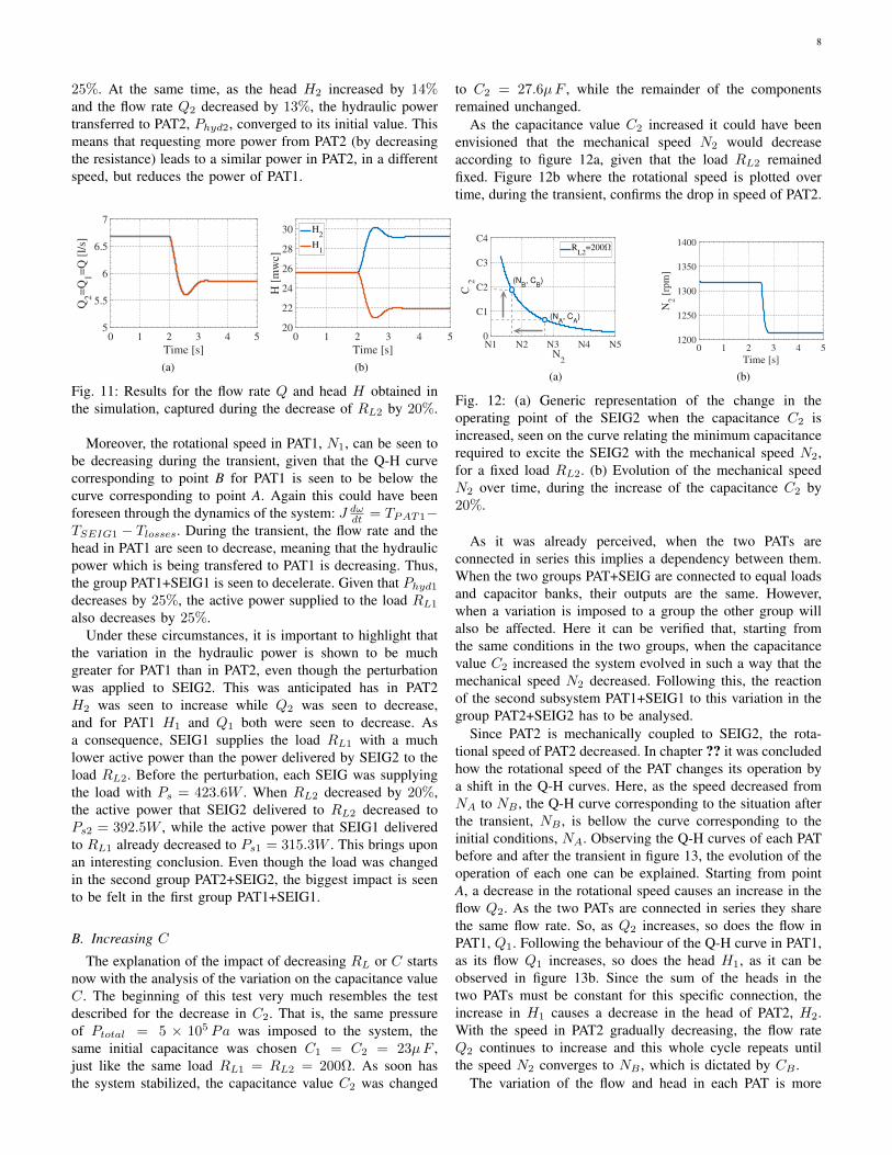
According to figure 11 the head and the flow both decreasein PAT1. The head is seen to decrease from 25.56 mwc to21.91 mwc, which corresponds to a variation of −14%. It canbe noticed here how H1 decreased 14% to compensate for theincrease in 14% of H2 in PAT2, given that the sum of bothheads is constant. Moreover, the flow is seen to decrease inthe two PATs from 6.69 l/s to 5.85 l/s, which corresponds to avariation of −13%. As a consequence of the decrease of 14%of the head H1 and the decrease of 13% of the flow rate Q1,the hydraulic power transferred to PAT1, Phyd1, decreased by

8

25%. At the same time, as the head H2 increased by 14%and the flow rate Q2 decreased by 13%, the hydraulic powertransferred to PAT2, Phyd2, converged to its initial value. Thismeans that requesting more power from PAT2 (by decreasingthe resistance) leads to a similar power in PAT2, in a differentspeed, but reduces the power of PAT1.

0 1 2 3 4 5

Time [s]

5

5.5

6

6.5

7

Q2=

Q1=

Q [

l/s]

(a)

0 1 2 3 4 5

Time [s]

20

22

24

26

28

30

H [

mw

c]

H2

H1

(b)

Fig. 11: Results for the flow rate Q and head H obtained inthe simulation, captured during the decrease of RL2 by 20%.

Moreover, the rotational speed in PAT1, N1, can be seen tobe decreasing during the transient, given that the Q-H curvecorresponding to point B for PAT1 is seen to be below thecurve corresponding to point A. Again this could have beenforeseen through the dynamics of the system: J dωdt = TPAT1−TSEIG1 − Tlosses. During the transient, the flow rate and thehead in PAT1 are seen to decrease, meaning that the hydraulicpower which is being transfered to PAT1 is decreasing. Thus,the group PAT1+SEIG1 is seen to decelerate. Given that Phyd1decreases by 25%, the active power supplied to the load RL1also decreases by 25%.

Under these circumstances, it is important to highlight thatthe variation in the hydraulic power is shown to be muchgreater for PAT1 than in PAT2, even though the perturbationwas applied to SEIG2. This was anticipated has in PAT2H2 was seen to increase while Q2 was seen to decrease,and for PAT1 H1 and Q1 both were seen to decrease. Asa consequence, SEIG1 supplies the load RL1 with a muchlower active power than the power delivered by SEIG2 to theload RL2. Before the perturbation, each SEIG was supplyingthe load with Ps = 423.6W . When RL2 decreased by 20%,the active power that SEIG2 delivered to RL2 decreased toPs2 = 392.5W , while the active power that SEIG1 deliveredto RL1 already decreased to Ps1 = 315.3W . This brings uponan interesting conclusion. Even though the load was changedin the second group PAT2+SEIG2, the biggest impact is seento be felt in the first group PAT1+SEIG1.

B. Increasing C

The explanation of the impact of decreasing RL or C startsnow with the analysis of the variation on the capacitance valueC. The beginning of this test very much resembles the testdescribed for the decrease in C2. That is, the same pressureof Ptotal = 5 × 105 Pa was imposed to the system, thesame initial capacitance was chosen C1 = C2 = 23µF ,just like the same load RL1 = RL2 = 200Ω. As soon hasthe system stabilized, the capacitance value C2 was changed

to C2 = 27.6µF , while the remainder of the componentsremained unchanged.

As the capacitance value C2 increased it could have beenenvisioned that the mechanical speed N2 would decreaseaccording to figure 12a, given that the load RL2 remainedfixed. Figure 12b where the rotational speed is plotted overtime, during the transient, confirms the drop in speed of PAT2.

N1 N2 N3 N4 N5

N2

0

C1

C2

C3

C4

C 2

RL2

=200

(NA, C

A)

(NB, C

B)

(a)

0 1 2 3 4 5

Time [s]

1200

1250

1300

1350

1400

N2 [

rpm

]

(b)

Fig. 12: (a) Generic representation of the change in theoperating point of the SEIG2 when the capacitance C2 isincreased, seen on the curve relating the minimum capacitancerequired to excite the SEIG2 with the mechanical speed N2,for a fixed load RL2. (b) Evolution of the mechanical speedN2 over time, during the increase of the capacitance C2 by20%.

As it was already perceived, when the two PATs areconnected in series this implies a dependency between them.When the two groups PAT+SEIG are connected to equal loadsand capacitor banks, their outputs are the same. However,when a variation is imposed to a group the other group willalso be affected. Here it can be verified that, starting fromthe same conditions in the two groups, when the capacitancevalue C2 increased the system evolved in such a way that themechanical speed N2 decreased. Following this, the reactionof the second subsystem PAT1+SEIG1 to this variation in thegroup PAT2+SEIG2 has to be analysed.

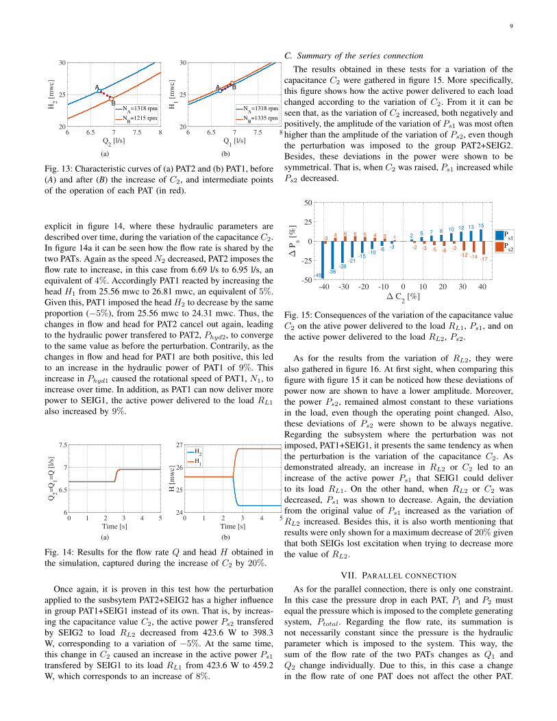
Since PAT2 is mechanically coupled to SEIG2, the rota-tional speed of PAT2 decreased. In chapter ?? it was concludedhow the rotational speed of the PAT changes its operation bya shift in the Q-H curves. Here, as the speed decreased fromNA to NB , the Q-H curve corresponding to the situation afterthe transient, NB , is bellow the curve corresponding to theinitial conditions, NA. Observing the Q-H curves of each PATbefore and after the transient in figure 13, the evolution of theoperation of each one can be explained. Starting from pointA, a decrease in the rotational speed causes an increase in theflow Q2. As the two PATs are connected in series they sharethe same flow rate. So, as Q2 increases, so does the flow inPAT1, Q1. Following the behaviour of the Q-H curve in PAT1,as its flow Q1 increases, so does the head H1, as it can beobserved in figure 13b. Since the sum of the heads in thetwo PATs must be constant for this specific connection, theincrease in H1 causes a decrease in the head of PAT2, H2.With the speed in PAT2 gradually decreasing, the flow rateQ2 continues to increase and this whole cycle repeats untilthe speed N2 converges to NB , which is dictated by CB .

The variation of the flow and head in each PAT is more

9

6 6.5 7 7.5 8

Q2 [l/s]

20

25

30

H2 [

mw

c]

A

BN

A=1318 rpm

NB

=1215 rpm

(a)

6 6.5 7 7.5 8

Q1 [l/s]

20

25

30

H1 [

mw

c]

A B

NA

=1318 rpm

NB

=1335 rpm

(b)

Fig. 13: Characteristic curves of (a) PAT2 and (b) PAT1, before(A) and after (B) the increase of C2, and intermediate pointsof the operation of each PAT (in red).

explicit in figure 14, where these hydraulic parameters aredescribed over time, during the variation of the capacitance C2.In figure 14a it can be seen how the flow rate is shared by thetwo PATs. Again as the speed N2 decreased, PAT2 imposes theflow rate to increase, in this case from 6.69 l/s to 6.95 l/s, anequivalent of 4%. Accordingly PAT1 reacted by increasing thehead H1 from 25.56 mwc to 26.81 mwc, an equivalent of 5%.Given this, PAT1 imposed the head H2 to decrease by the sameproportion (−5%), from 25.56 mwc to 24.31 mwc. Thus, thechanges in flow and head for PAT2 cancel out again, leadingto the hydraulic power transfered to PAT2, Phyd2, to convergeto the same value as before the perturbation. Contrarily, as thechanges in flow and head for PAT1 are both positive, this ledto an increase in the hydraulic power of PAT1 of 9%. Thisincrease in Phyd1 caused the rotational speed of PAT1, N1, toincrease over time. In addition, as PAT1 can now deliver morepower to SEIG1, the active power delivered to the load RL1also increased by 9%.

0 1 2 3 4 5

Time [s]

6

6.5

7

7.5

Q2=

Q1=

Q [

l/s]

(a)

0 1 2 3 4 5

Time [s]

24

25

26

27

H [

mw

c]

H2

H1

(b)

Fig. 14: Results for the flow rate Q and head H obtained inthe simulation, captured during the increase of C2 by 20%.

Once again, it is proven in this test how the perturbationapplied to the susbsytem PAT2+SEIG2 has a higher influencein group PAT1+SEIG1 instead of its own. That is, by increas-ing the capacitance value C2, the active power Ps2 transferedby SEIG2 to load RL2 decreased from 423.6 W to 398.3W, corresponding to a variation of −5%. At the same time,this change in C2 caused an increase in the active power Ps1transfered by SEIG1 to its load RL1 from 423.6 W to 459.2W, which corresponds to an increase of 8%.

C. Summary of the series connection

The results obtained in these tests for a variation of thecapacitance C2 were gathered in figure 15. More specifically,this figure shows how the active power delivered to each loadchanged according to the variation of C2. From it it can beseen that, as the variation of C2 increased, both negatively andpositively, the amplitude of the variation of Ps1 was most oftenhigher than the amplitude of the variation of Ps2, even thoughthe perturbation was imposed to the group PAT2+SEIG2.Besides, these deviations in the power were shown to besymmetrical. That is, when C2 was raised, Ps1 increased whilePs2 decreased.

-3-6

-10-15

25 7

12 13 15

8 10

-21

-28

-36-48

1345

-2 -3 -5

-12 -14-17

-6-3

664-3

-40 -30 -20 -10 0 10 20 30 40

C2 [%]

-50

-25

0

25

50

Ps [

%]

Ps1

Ps2

Fig. 15: Consequences of the variation of the capacitance valueC2 on the ative power delivered to the load RL1, Ps1, and onthe active power delivered to the load RL2, Ps2.

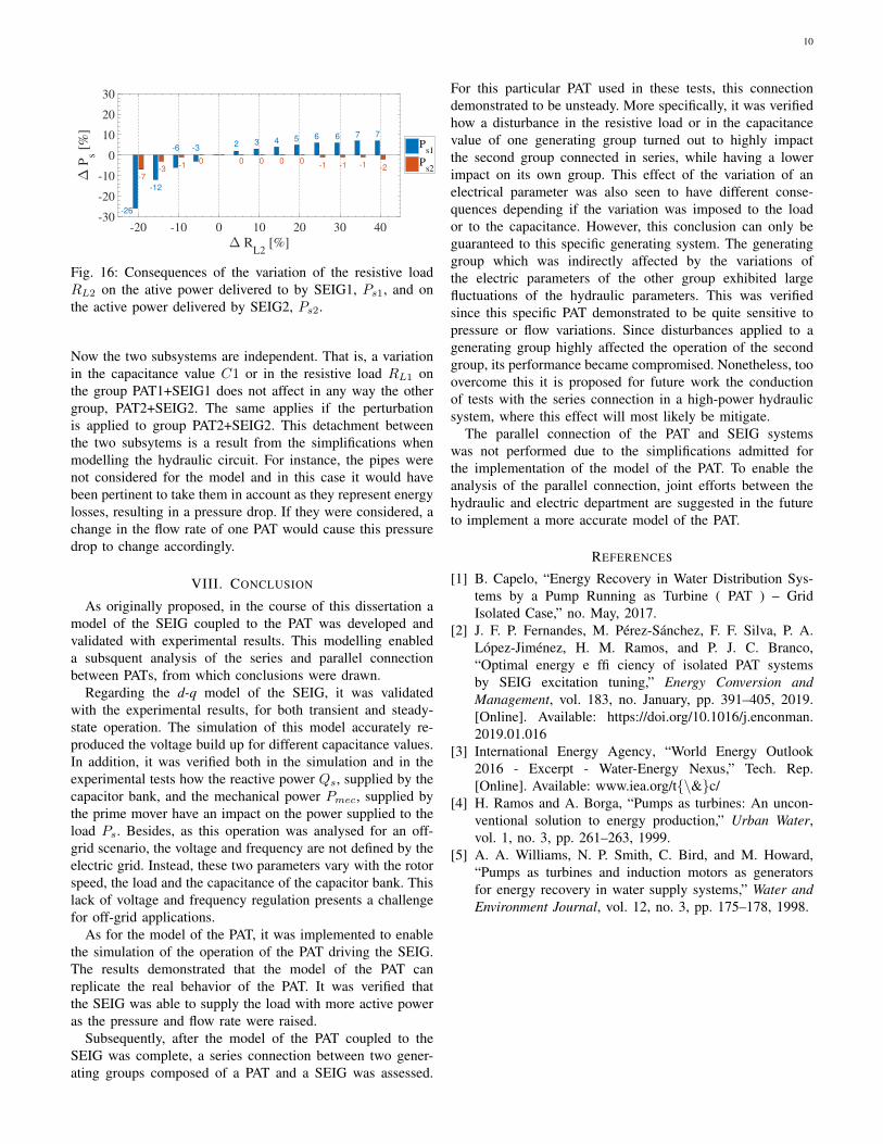
As for the results from the variation of RL2, they werealso gathered in figure 16. At first sight, when comparing thisfigure with figure 15 it can be noticed how these deviations ofpower now are shown to have a lower amplitude. Moreover,the power Ps2, remained almost constant to these variationsin the load, even though the operating point changed. Also,these deviations of Ps2 were shown to be always negative.Regarding the subsystem where the perturbation was notimposed, PAT1+SEIG1, it presents the same tendency as whenthe perturbation is the variation of the capacitance C2. Asdemonstrated already, an increase in RL2 or C2 led to anincrease of the active power Ps1 that SEIG1 could deliverto its load RL1. On the other hand, when RL2 or C2 wasdecreased, Ps1 was shown to decrease. Again, the deviationfrom the original value of Ps1 increased as the variation ofRL2 increased. Besides this, it is also worth mentioning thatresults were only shown for a maximum decrease of 20% giventhat both SEIGs lost excitation when trying to decrease morethe value of RL2.

VII. PARALLEL CONNECTION

As for the parallel connection, there is only one constraint.In this case the pressure drop in each PAT, P1 and P2 mustequal the pressure which is imposed to the complete generatingsystem, Ptotal. Regarding the flow rate, its summation isnot necessarily constant since the pressure is the hydraulicparameter which is imposed to the system. This way, thesum of the flow rate of the two PATs changes as Q1 andQ2 change individually. Due to this, in this case a changein the flow rate of one PAT does not affect the other PAT.

10

0 0 0 0 0

-3-6

-12

-26

2 3 46 7 7

5 6

-1-3

-7

-1 -1 -2-1

-20 -10 0 10 20 30 40

RL2

[%]

-30

-20

-10

0

10

20

30 P

s [%

]

Ps1

Ps2

Fig. 16: Consequences of the variation of the resistive loadRL2 on the ative power delivered to by SEIG1, Ps1, and onthe active power delivered by SEIG2, Ps2.

Now the two subsystems are independent. That is, a variationin the capacitance value C1 or in the resistive load RL1 onthe group PAT1+SEIG1 does not affect in any way the othergroup, PAT2+SEIG2. The same applies if the perturbationis applied to group PAT2+SEIG2. This detachment betweenthe two subsytems is a result from the simplifications whenmodelling the hydraulic circuit. For instance, the pipes werenot considered for the model and in this case it would havebeen pertinent to take them in account as they represent energylosses, resulting in a pressure drop. If they were considered, achange in the flow rate of one PAT would cause this pressuredrop to change accordingly.

VIII. CONCLUSION

As originally proposed, in the course of this dissertation amodel of the SEIG coupled to the PAT was developed andvalidated with experimental results. This modelling enableda subsquent analysis of the series and parallel connectionbetween PATs, from which conclusions were drawn.

Regarding the d-q model of the SEIG, it was validatedwith the experimental results, for both transient and steady-state operation. The simulation of this model accurately re-produced the voltage build up for different capacitance values.In addition, it was verified both in the simulation and in theexperimental tests how the reactive power Qs, supplied by thecapacitor bank, and the mechanical power Pmec, supplied bythe prime mover have an impact on the power supplied to theload Ps. Besides, as this operation was analysed for an off-grid scenario, the voltage and frequency are not defined by theelectric grid. Instead, these two parameters vary with the rotorspeed, the load and the capacitance of the capacitor bank. Thislack of voltage and frequency regulation presents a challengefor off-grid applications.

As for the model of the PAT, it was implemented to enablethe simulation of the operation of the PAT driving the SEIG.The results demonstrated that the model of the PAT canreplicate the real behavior of the PAT. It was verified thatthe SEIG was able to supply the load with more active poweras the pressure and flow rate were raised.

Subsequently, after the model of the PAT coupled to theSEIG was complete, a series connection between two gener-ating groups composed of a PAT and a SEIG was assessed.

For this particular PAT used in these tests, this connectiondemonstrated to be unsteady. More specifically, it was verifiedhow a disturbance in the resistive load or in the capacitancevalue of one generating group turned out to highly impactthe second group connected in series, while having a lowerimpact on its own group. This effect of the variation of anelectrical parameter was also seen to have different conse-quences depending if the variation was imposed to the loador to the capacitance. However, this conclusion can only beguaranteed to this specific generating system. The generatinggroup which was indirectly affected by the variations ofthe electric parameters of the other group exhibited largefluctuations of the hydraulic parameters. This was verifiedsince this specific PAT demonstrated to be quite sensitive topressure or flow variations. Since disturbances applied to agenerating group highly affected the operation of the secondgroup, its performance became compromised. Nonetheless, tooovercome this it is proposed for future work the conductionof tests with the series connection in a high-power hydraulicsystem, where this effect will most likely be mitigate.

The parallel connection of the PAT and SEIG systemswas not performed due to the simplifications admitted forthe implementation of the model of the PAT. To enable theanalysis of the parallel connection, joint efforts between thehydraulic and electric department are suggested in the futureto implement a more accurate model of the PAT.

REFERENCES

[1] B. Capelo, “Energy Recovery in Water Distribution Sys-tems by a Pump Running as Turbine ( PAT ) – GridIsolated Case,” no. May, 2017.

[2] J. F. P. Fernandes, M. Perez-Sanchez, F. F. Silva, P. A.Lopez-Jimenez, H. M. Ramos, and P. J. C. Branco,“Optimal energy e ffi ciency of isolated PAT systemsby SEIG excitation tuning,” Energy Conversion andManagement, vol. 183, no. January, pp. 391–405, 2019.[Online]. Available: https://doi.org/10.1016/j.enconman.2019.01.016

[3] International Energy Agency, “World Energy Outlook2016 - Excerpt - Water-Energy Nexus,” Tech. Rep.[Online]. Available: www.iea.org/t\&c/

[4] H. Ramos and A. Borga, “Pumps as turbines: An uncon-ventional solution to energy production,” Urban Water,vol. 1, no. 3, pp. 261–263, 1999.

[5] A. A. Williams, N. P. Smith, C. Bird, and M. Howard,“Pumps as turbines and induction motors as generatorsfor energy recovery in water supply systems,” Water andEnvironment Journal, vol. 12, no. 3, pp. 175–178, 1998.