Embed Size (px)
Citation preview
Punjab UniversityJournal of Mathematics (ISSN 1016-2526) Vol. 51(5)(2019) pp. 79-95
A Numerical Approach of Slip Conditions Effect on Nanofluid Flow over aStretching Sheet under Heating Joule Effect
Hafiz Abdul Wahab1∗, Hussan Zeb1, Saira Bhatti2 Muhammad Gulistan1 and SarfarazAhmad3
1Department of Mathematics & Statistics, Hazara University, Mansehra2Department of Mathematics, COMSATS University Islamabad, Abbottabad Campus
3Department of Mathematics, AUST, AbbottabadEmail corresponding author: [email protected]
Received: 03 September, 2018 / Accepted: 09 November, 2018 / Published online: 05March, 2019
Abstract. In this analysis, we considered the effects of Joule heatingand partial slip boundary conditions on time dependent mixed convectivenanofluid flow over a stretching sheet along with heat source/sink. Thegoverning model is transformed into the system of nonlinear ODE’s byusing the well known transformations. In order to calculate the physicalquantities of the problem, we use the higher order convergence method,called shotting method followed by Runge-Kutta Fehlberg method. Theimportance of different physical parameters on velocity, temperature andconcentration profiles are calculated numerically. The parameters of en-gineering interest i.e, skin fraction, Nusselt and Sherwood numbers arealso calculated. Finally, we concluded that the velocity profiles decreaseby increasing values of A and M . Moreover the variation of temperature,velocity and concentration profiles are analyzed for the different physicalparameters.
AMS (MOS) Subject Classification Codes: 35S29; 40S70; 25U09Key Words: Shooting method; MHD boundary layer flow; nanofluid flow; Joule heating;
partial slip conditions.
1. INTRODUCTION
The investigation of the boundary layer pseudo plastic fluids has been of a great inter-est because it has many practical usage in industry such as emulsion coated sheets like photographic film, extrusion of polymer sheets, e tc. In order to examine the rheological assents of fluids, the Navier-Stokes equations are insufficient alone. Therefore, rheological models are implemented to reduced this problem. The description of non-Newtonian fluids
79
80 Hafiz Abdul Wahab, Hussan Zeb, Saira Bhatti, Muhammad Gulistan and Sarfaraz Ahmad
does not exist in single constitutive relationship between stress and strain. Due to their in-dustrial and physiological applications, the non-Newtonian fluids have gained tremendousattraction. A plenty of applications in various built-up processing and biological fluids, aninterest in boundary layer non-Newtonian fluid is increased significantly. A Few examplesare drilling mud, plastic polymer, hot rolling, optical fibers, metal spinning, paper produc-tion and cooling of metallic plates. The investigation of the flow due to extending surfacein a moving liquid is important in advanced industry. For example, the expulsion of met-als and plastics, glass blowing, cooling or drying of papers, etc. The problems of linearstretching sheet for many events of fluid have also been investigated by many researchers.Sakiadis et al. [34] examined the boundary layer flow over a stretching surface. Variousauthors have discussed the different feathers of the flow over a movable plats. Vleggaar[36] studied the boundary layer on the stretching surface almost proportional to the dis-tance from the orifice. Carn [14] studied Newtonian fluid flow layer over a stretching sheeton the uniform stress.
The magnetohydrodynomics of an electrically conducting fluid is an important phenom-ena used in metallurgical and modern metal-working. The electrical furnace metal can befused by using the magnetic field and In a nuclear reactor containment boat, the wall ofnuclear reactor is cooled down by applying magnetic field. MHD term was first proposedby Swedish electrical engineer, Alfve [5] in 1942. MHD equations are the combinationof Maxwell’s equations of electromagnetism, continuity equation and Navier-Stokes equa-tions. If the electrically conducting liquid placed in a static magnetic field, the fluid move-ment pushes currents that create forces on the fluid. Equations that describe the MHD floware a mixture of continuity equation, Navier Stokes equations and Maxwell’s equations influid dynamics. Zeb et al. [39] we studied the effect of thermal radiation on time de-pendent fluid flow over a stretching sheet with variable thermal conductivity. Zeb et al.[40] studied the effect of thermal radiation and slip boundary condition on time depen-dent fluid flow over a stretching sheet along with variable thermal conductivity. Hussain etal. [20]investigated the impact of thermal radiation on bioconversions model for magneto-hydrodynamics squeezing flow of nanofluid with heat and mass transfer between parallelsurface.Time dependent MHD oscillating and rotating flow of Maxwell fluid in a cylindersubject to shear stress on the boundary was analyzed by Zafar et al. [38]. Mukhopadhyayet al. [25] investigated the effects of Joule heating on magnetohydrodynamics Newtonianfluid flow over a stretching sheet by placing between suction and junction. Raju et al.[30] analyzed the MHD free convective with pours medium by taking horizontal channelassuming insolated and incompressible bottom wall with the effect of heating joule andviscous dissipation. Ahmad et al. [4] examined quasi-linearization for unsteady MHD inheat and mass transfer flow of nanofluid overastreachin sheet. Huichu [19] analyzed the un-steady MHD boundary layer flow over a stretching sheet along with frictional and Ohmicheating. Malik, et al. [23] investigated the magnetohydrodynamics stagnation point flowover a stretching sheet by assuming the convective boundary condition. MHD time depen-dent flow of a burger fluid past a circular cylinder along with porous medium was studiedSafadar et al. [32] . the chemically reacting of incompressible fluid over an vertical plateswas discussed by Awan et al. [9]. Sadiq et al. [33] discussed the exact solution of unsteadyflow of Oldroyed-B fluid placed in a circular cylinder. Awan [8] analysed the exact solutionfor the time dependent flow of Maxwell fluid is placed in coaxial cylinder. Ali et al. [6]
A Numerical Approach of the Slip Conditions Effect on Nanofluid Flow over a Stretching Sheet under Heating Joule Effect 81
investigated the influence of Magnetohydrodynamic electrically conducting oscillating andRotating flows of Maxwell Fluids in a porous medium.
Another type of fluid is nanofluids which is measured by dispersing of small sized ma-terials such as nanotubes, nanofibers, nanowires, droplets, nanosheet and nanorods. Thenano-fluids are nanoscale colloidal suspensions containing condensed nanomaterials. Thestudy of nanofluids has been a topic of intense research during the last one decade dueto their interesting thermophysical properties and anticipated applications in heat transfer.The thermal conductivity of equal sample colloidally stable dispersed of nanofluids wereobtained by using different experimental methods reported by the International NanofluidProperty Benchmark Exercise (INPBE). Nanotechnology has been commonly used in en-gineering since materials with size of nanometers possess unique chemical and physicalproperties. Tested nanofluids in the above study were based on aqueous and nonaqueousbase-fluids and many others. In the above analysis, the data has been taken from most ofthe organization with in a relativity narrow based (±10% or below) about the sample meanwith little outliers. It is found that the thermal conductivity of nano-fluids enlarges with in-crease in particle concentration and aspect ratio, as expected from classical theory, amongvarious experimental approaches; small systematic differences in the absolute values of thenano-fluid thermal conductivity are obtained while such differences tend to disappear whenthe data are normalized to measure thermal conductivity of the base-fluids. Further expla-nation can be found in work by Jacopo et al. [11]. The evaluation of convective boundaryconditions on MHD boundary layer nanofluid over a stretching sheet was found by Ishak etal. [10]. The steady flow of a third grade fluid in a porous half space was found by Karimiet al. [21] via rational Bernstein collocation method.
The phenomena of velocity slip has been discussed under different cases by using non-adherence of the fluid to solid boundary in [37]. Time dependent rotational flow of a secondgrad fluid with caputo time fractional deriavtive was examined by Raza et al. [31]. Theviscous fluid is normally sticks to the boundary, for example, particulate fluid, rare fieldgas and many more which are discussed in [35]. The consequences of the slip conditionplays a vital rule in the field of scientific, industrial and biological applications such asthe internal cavities and artificial polishing of heart valves [24]. The most important studytaken into the account is the slip boundary conditions over stretching sheets were carriedout by Anderson [7]. Ibrahim et al. [17] analyzed manatohydrodynamics boundary layerflow and heat transfer of nanofluid by assuming permeable stretching sheet taking the effectof slip boundary conditions. Poornima et al. [28] find out the effect of radiation on convec-tion boundary layer flow due to a non linear stretching sheet. Rmaa Bhargava and ManiaGoyal [12] simulate the consequences of velocity slip on MHD nanofluid with heat gener-ation over a stretching sheet. The event of entropy generation on magnetohydrodynamicsnanofluid flow over a stretching sheet under the considering velocity slip condition withheat generation was found out by Govindaraju et al. in [16]. Malik et al. [22] explainedthe manatohydrodynamics and mixed convection flow of Eyring-Powell nanofluid by as-suming the stretching sheet. Ndeem et al. [26] proposed a numerical studied viscoelasticnanofluid for two-dimensional stagnation point flow. They found influence of the embed-ded parameters. They used viscoelastic nanofluid for the controlling heat transfer from thesheet. Therefore, many ways were taken for improving the thermal conductivity of thesefluids through suspension nano/micro or large-sized material particles in the fluid. Duwairi
82 Hafiz Abdul Wahab, Hussan Zeb, Saira Bhatti, Muhammad Gulistan and Sarfaraz Ahmad
[15] discussed the influence of Joule heating on the forced convection flow with thermal ra-diation. Partha et al. [27] reported that the events of the radiation on mixed convection heattransfer from an exponentially stretching surface under the consideration of viscous dissi-pation. Abro et al. [2] analyzed MHD generalized burger fluid over a permeable plates.Reddy [29] studied the viscous dissipation and thermal radiation on MHD flow due to astretching sheet. MHD second grade unsteady flow of heat transfer with porous mediumby using caputo-fabrizoi fractional derivative was found by Abro et al. [1]. Abelman etal. [3]. analyzed the analytical solution of magnatohydrodynomics rotating and oscillatingflow of a Maxwell fluid electrically conducting in a porous medium. Bhuiyan et al. [13]reported the Joule heating effects on MHD natural convection flows being with viscousdissipation from a horizontal circular cylinder. Ishaq et al. [18] examined time dependentMHD flow nanofluid film of an eyring Powell Fluid over a porous Stretching Sheet
From the above literature review, it is confirmed that no attempt has been made to theeffect of heat source/sink on time dependent mixed convective nanofluid and heat transferover a stretching sheet with Joule heating. We have successfully computed the solution ofthe coupled ordinary differential equations via numerical scheme through shooting methodfollowed by Runge-Kutta Fehlberg method. The variation of different physical aspects arepresented through graphs. Also, we obtained the numerical results for local skin fraction,heat transfer rate and Sherwood number by various different parameters (discussed in ta-bles).
2. MATHEMATICAL MODEL
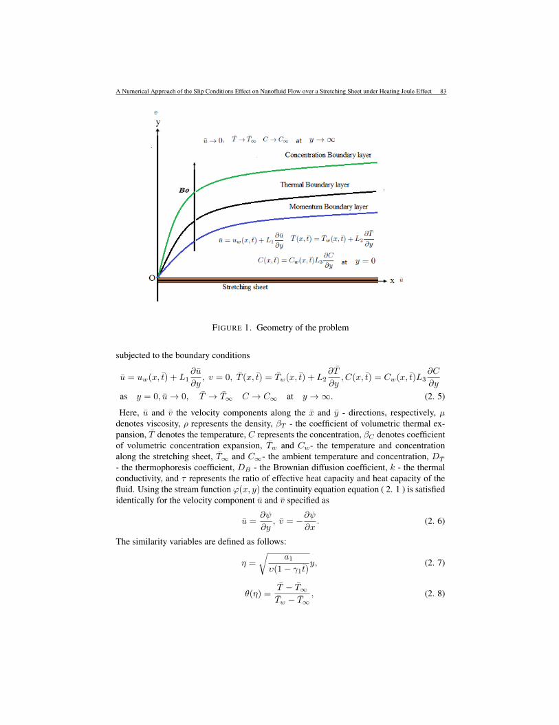
Let us consider an unsteady MHD incompressible mixed convective Nano-fluid flowover a stretching sheet along with partial slip condition. The flow is produced by a stretch-ing sheet. The flow is in the region y > 0 and subjected to a non-uniform magnetic fieldof strength B = B0
√1− γ1t applied normally to the sheet, B0 is the initial strength of
the magnetic field; see in the Fig 1. The fluid and heat flows are initiated at time zero. Thesheet emerges out of a slit at origin x = 0, y = 0 and moves with non-uniform velocityuw(x, t) = a1x
1−γ1 t , where a1 and γ1 are positive constants with dimensions of t−1, and a1
is the initial stretching rate.
∂u
∂x+∂v
∂y= 0, (2. 1)
∂u
∂t+ u
∂u
∂x+ v
∂v
∂y= ν
∂2u
∂2y− σβ2u
ρ+ [βT (T − T∞) + βC(C − C∞)]g, (2. 2)
∂T
∂t+ u
∂T
∂x+ v
∂T
∂y=
k
ρcp
∂2T
∂y2+ σ
B20
ρu2 + τ [DB(
∂C
∂y
∂C
∂y) + (
DT
T∞)(∂T
∂y)2]
+Q
ρcp(T − T∞), (2. 3)
∂C
∂t+ u
∂C
∂x+∂T
∂y= DB(
∂2C
∂2y) + τ [DB(
DT
T∞)(∂2T
∂y2) (2. 4)
A Numerical Approach of the Slip Conditions Effect on Nanofluid Flow over a Stretching Sheet under Heating Joule Effect 83
FIGURE 1. Geometry of the problem
subjected to the boundary conditions
u = uw(x, t) + L1∂u
∂y, v = 0, T (x, t) = Tw(x, t) + L2
∂T
∂y, C(x, t) = Cw(x, t)L3
∂C
∂y
as y = 0, u→ 0, T → T∞ C → C∞ at y →∞. (2. 5)
Here, u and v the velocity components along the x and y - directions, respectively, µdenotes viscosity, ρ represents the density, βT - the coefficient of volumetric thermal ex-pansion, T denotes the temperature, C represents the concentration, βC denotes coefficientof volumetric concentration expansion, Tw and Cw- the temperature and concentrationalong the stretching sheet, T∞ and C∞- the ambient temperature and concentration, DT
- the thermophoresis coefficient, DB - the Brownian diffusion coefficient, k - the thermalconductivity, and τ represents the ratio of effective heat capacity and heat capacity of thefluid. Using the stream function ϕ(x, y) the continuity equation equation ( 2. 1 ) is satisfiedidentically for the velocity component u and v specified as
u =∂ψ
∂y, v = −∂ψ
∂x. (2. 6)
The similarity variables are defined as follows:
η =
√a1
υ(1− γ1t)y, (2. 7)
θ(η) =T − T∞Tw − T∞
, (2. 8)
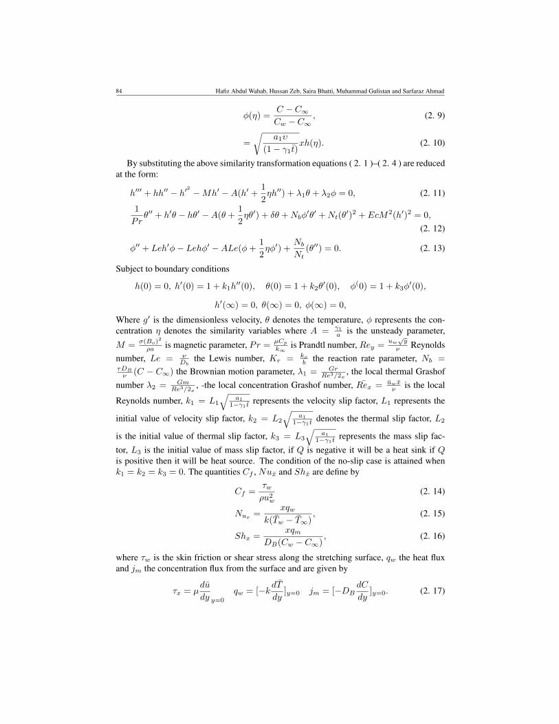
84 Hafiz Abdul Wahab, Hussan Zeb, Saira Bhatti, Muhammad Gulistan and Sarfaraz Ahmad
φ(η) =C − C∞Cw − C∞
, (2. 9)
=
√a1υ
(1− γ1t)xh(η). (2. 10)
By substituting the above similarity transformation equations ( 2. 1 )–( 2. 4 ) are reducedat the form:
h′′′ + hh′′ − h′2
−Mh′ −A(h′ +1
2ηh′′) + λ1θ + λ2φ = 0, (2. 11)
1
Prθ′′ + h′θ − hθ′ −A(θ +
1
2ηθ′) + δθ +Nbφ
′θ′ +Nt(θ′)2 + EcM2(h′)2 = 0,
(2. 12)
φ′′ + Leh′φ− Lehφ′ −ALe(φ+1
2ηφ′) +
NbNt
(θ′′) = 0. (2. 13)
Subject to boundary conditions
h(0) = 0, h′(0) = 1 + k1h′′(0), θ(0) = 1 + k2θ
′(0), φ(0) = 1 + k3φ′(0),
h′(∞) = 0, θ(∞) = 0, φ(∞) = 0,
Where g′ is the dimensionless velocity, θ denotes the temperature, φ represents the con-centration η denotes the similarity variables where A = γ1
a is the unsteady parameter,
M = σ(Bo)2
ρa is magnetic parameter, Pr =µCp
k∞is Prandtl number, Rey =
uw√y
ν Reynoldsnumber, Le = ν
Dbthe Lewis number, Kr = ko
b the reaction rate parameter, Nb =τDB
ν (C − C∞) the Brownian motion parameter, λ1 = GrRe3/2x
, the local thermal Grashofnumber λ2 = Gm
Re3/2x, -the local concentration Grashof number, Rex = uwx
ν is the local
Reynolds number, k1 = L1
√a1
1−γ1 t represents the velocity slip factor, L1 represents the
initial value of velocity slip factor, k2 = L2
√a1
1−γ1 t denotes the thermal slip factor, L2
is the initial value of thermal slip factor, k3 = L3
√a1
1−γ1 t represents the mass slip fac-
tor, L3 is the initial value of mass slip factor, if Q is negative it will be a heat sink if Qis positive then it will be heat source. The condition of the no-slip case is attained whenk1 = k2 = k3 = 0. The quantities Cf , Nux and Shx are define by
Cf =τwρu2
w
(2. 14)
Nux =xqw
k(Tw − T∞), (2. 15)
Shx =xqm
DB(Cw − C∞), (2. 16)
where τw is the skin friction or shear stress along the stretching surface, qw the heat fluxand jm the concentration flux from the surface and are given by
τx = µdu
dy y=0
qw = [−kdTdy
]y=0 jm = [−DBdC
dy]y=0. (2. 17)
A Numerical Approach of the Slip Conditions Effect on Nanofluid Flow over a Stretching Sheet under Heating Joule Effect 85
where uw qm and qw, are the wall shear stress, mass fluxes and heat transfer respectively.In dimensionless form, In dimensionless form, the reduced local Nusselt and Sherwoodnumbers can be written as
Cf√Rex = h′′(0),
Nux√Rex
= −θ′(0),Shx√Rex
= −φ′(0). (2. 18)
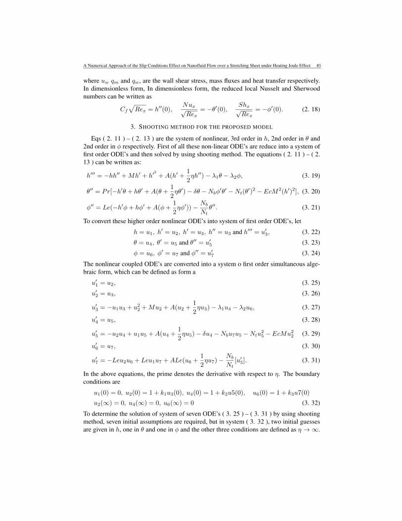
3. SHOOTING METHOD FOR THE PROPOSED MODEL
Eqs ( 2. 11 ) – ( 2. 13 ) are the system of nonlinear, 3rd order in h, 2nd order in θ and2nd order in φ respectively. First of all these non-linear ODE’s are reduce into a system offirst order ODE’s and then solved by using shooting method. The equations ( 2. 11 ) – ( 2.13 ) can be written as:
h′′′ = −hh′′ +Mh′ + h′2
+A(h′ +1
2ηh′′)− λ1θ − λ2φ, (3. 19)
θ′′ = Pr[−h′θ + hθ′ +A(θ +1
2ηθ′)− δθ −Nbφ′θ′ −Nt(θ′)2 − EcM2(h′)2], (3. 20)
φ′′ = Le(−h′φ+ hφ′ +A(φ+1
2ηφ′))− Nb
Ntθ′′. (3. 21)
To convert these higher order nonlinear ODE’s into system of first order ODE’s, let
h = u1, h′ = u2, h
′ = u3, h′′ = u3 and h′′′ = u′3, (3. 22)
θ = u4, θ′ = u5 and θ′′ = u′5 (3. 23)
φ = u6, φ′ = u7 and φ′′ = u′7 (3. 24)
The nonlinear coupled ODE’s are converted into a system o first order simultaneous alge-braic form, which can be defined as form a
u′1 = u2, (3. 25)
u′2 = u3, (3. 26)
u′3 = −u1u3 + u22 +Mu2 +A(u2 +
1
2ηu3)− λ1u4 − λ2u6, (3. 27)
u′4 = u5, (3. 28)
u′5 = −u2u4 + u1u5 +A(u4 +1
2ηu5)− δu4 −Nbu7u5 −Ntu2
5 − EcMu22 (3. 29)
u′6 = u7, (3. 30)
u′7 = −Leu2u6 + Leu1u7 +ALe(u6 +1
2ηu7)− Nb
Nt[u′5]. (3. 31)
In the above equations, the prime denotes the derivative with respect to η. The boundaryconditions are
u1(0) = 0, u2(0) = 1 + k1u3(0), u4(0) = 1 + k2u5(0), u6(0) = 1 + k3u7(0)
u2(∞) = 0, u4(∞) = 0, u6(∞) = 0 (3. 32)
To determine the solution of system of seven ODE’s ( 3. 25 ) – ( 3. 31 ) by using shootingmethod, seven initial assumptions are required, but in system ( 3. 32 ), two initial guessesare given in h, one in θ and one in φ and the other three conditions are defined as η →∞.
86 Hafiz Abdul Wahab, Hussan Zeb, Saira Bhatti, Muhammad Gulistan and Sarfaraz Ahmad
These three conditions generate result in three unknowns. The subsequent and foremoststep of this method is choosing the estimated values of η at ∞. The solution processis initiated with certain initial guesses and finding out the solution of (BVP) includinggoverning model. The method of solution with a new values of η at η → ∞ and themethod is repeated until two consecutive values of g′′(0), θ′(0) and φ′(0) are different onlyafter the significant digits. Thus final values of η are considered as η →∞.
4. RESULTS AND DISCUSSION
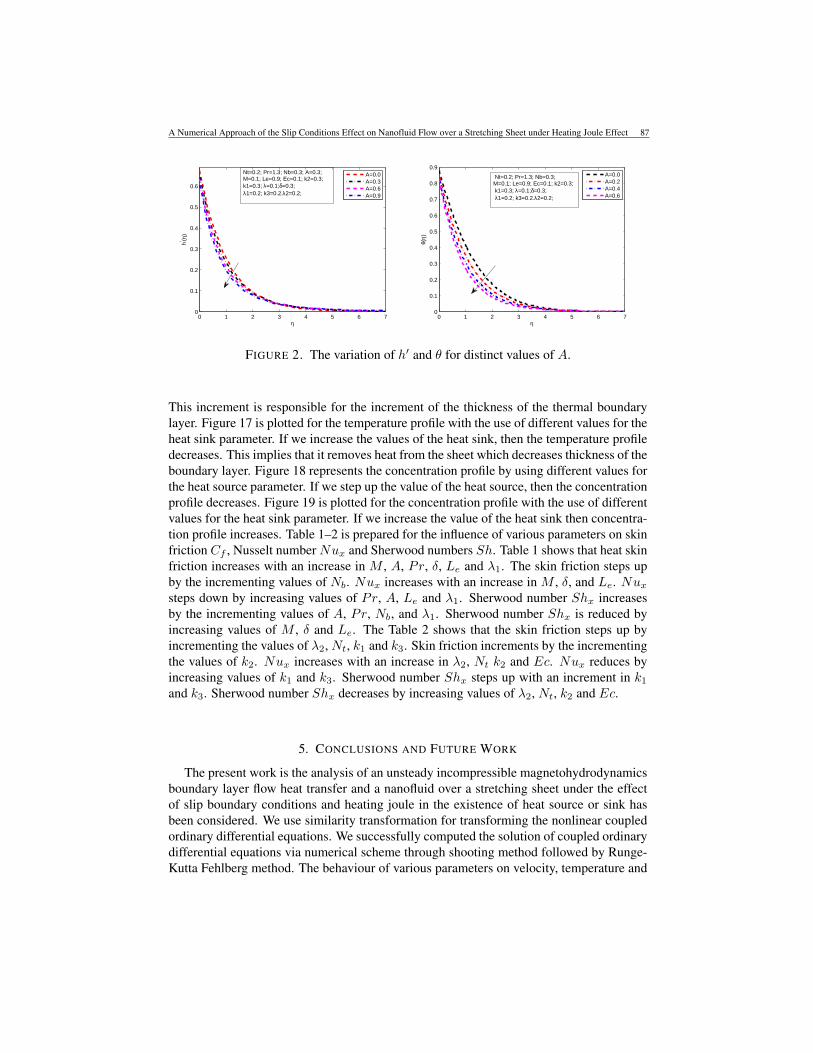
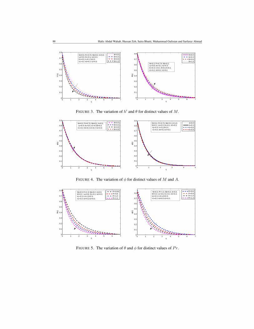
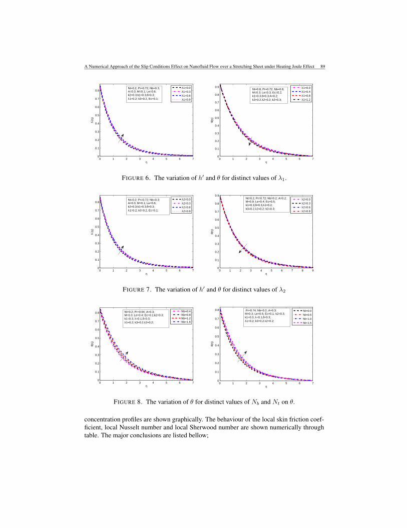
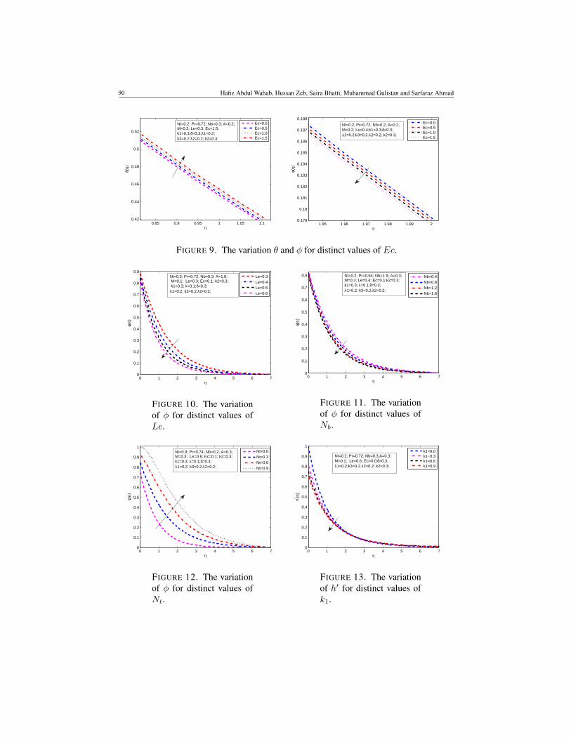
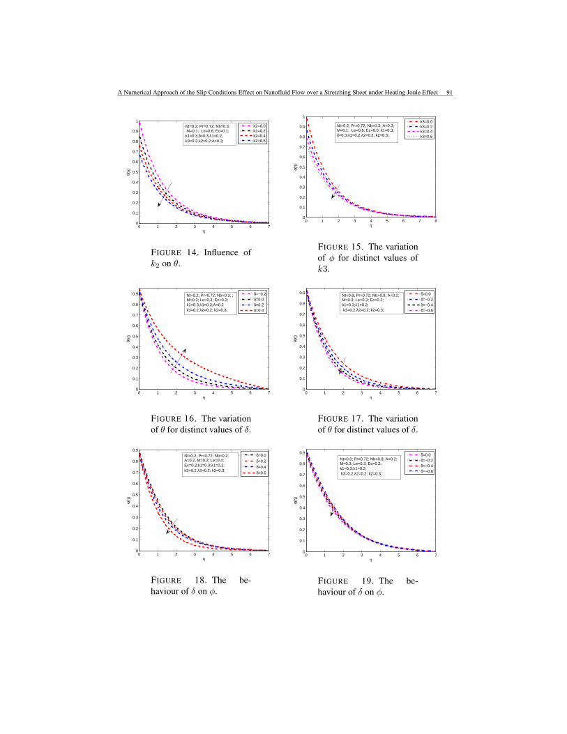
The variation of different physical aspects are presented through graphs (as shown inFigs 2–19). The influence of unsteady parameter is shown in Fig: 2 on the velocity andtemperature profiles. Fig 3 is for the variation of velocity and temperature profiles for val-ues of M . A decrease in variation of velocity and temperature profiles increases by enlargevalues of M . Fig: 4 plotted for the distribution of concentration profile for the distinct val-ues of M and A respectively. The decreases the concentration profile by increasing valuesof M and A. Figure 5 plotted for the distribution of concentration and temperature profilesfor the distinct values of Pr. The temperature profile decreases and concentration profileincreases by increasing values of Pr. Figure 6 designated for the velocity and temperatureprofiles for the different values of λ1. The increase in the velocity profile and decreasein temperature profile by increasing the values of λ1. Figure 7 indicates the variation ofvelocity and temperature profiles for the various values of λ2. The result has shown thestep down the velocity and temperature profiles by the step up values of λ2. Figure 8 showsthe distribution of the temperature profile for the various values of the Nt and Nb. The re-sult has show that the temperature profile decreases by increasing values of thermophoresisNt and Brownian motion parameters Nb. The Figure 9 shows that the influence of Eckletnumber Ec on temperature and concentration profiles. The result shows that the temper-ature profile increases and reduced the concentration profile by the step up values of Ec.Figure 10 designated for the distribution of the concentration profile for values of Le onthe concentration profile. The result shows that a decrease in concentration profile as theLe increases. This is due to the fact that there is a decrease in the nanoparticle volumefraction boundary layer thickness with the increase in the Lewis number. Figure 11 showsthe variation of the concentration profile for the distinct values of Nb. It is noticed thatthe concentration profile is reduced by incrementing value in Brownian motion Nb. Theeffect of the thermophoresis parameter Nt on the concentration of the flow field is show inFigure 12. We observe that the behavior of Nt indicates a cold surface while negative toa hot surface. It is seen that the concentration decreases, as the thermophoresis parameterincreases. The variation of velocity slip parameter k1 on the velocity profile is shown inFigure 13. The result shows that the velocity graph is reduced with the step up values ofvelocity slip parameter k1. Figure 14 is plotted for the distinction of the temperature profilefor the different values thermal slip parameter k2. On observing this figure, the temperaturegraph is reduced as the value of temperature slip parameter k2 increase. Figure 15 is plottedfor the influence of the solutal slip parameter k3 on the concentration profile. The result hasshown that the concentration profile is reduced by the step up value of solutal slip parame-ter k3. Figure 16 represents the temperature profile with using different value for the heatsource parameter. If we increase the value of the heat source, then the temperature profileincreases. Heat source provides extra heat to the sheet which increases its temperature.
A Numerical Approach of the Slip Conditions Effect on Nanofluid Flow over a Stretching Sheet under Heating Joule Effect 87
0 1 2 3 4 5 6 70
0.1
0.2
0.3
0.4
0.5
0.6h′ (η
)
η
A=0.0A=0.3A=0.6A=0.9
Nt=0.2; Pr=1.3; Nb=0.3; A=0.3;M=0.1; Le=0.9; Ec=0.1; k2=0.3;k1=0.3; λ=0.1;δ=0.3;λ1=0.2; k3=0.2.λ2=0.2;
0 1 2 3 4 5 6 70
0.1
0.2
0.3
0.4
0.5
0.6
0.7
0.8
0.9
θ(η)
η
A=0.0A=0.2A=0.4A=0.6
Nt=0.2; Pr=1.3; Nb=0.3;M=0.1; Le=0.9; Ec=0.1; k2=0.3; k1=0.3; λ=0.1;δ=0.3; λ1=0.2; k3=0.2.λ2=0.2;
FIGURE 2. The variation of h′ and θ for distinct values of A.
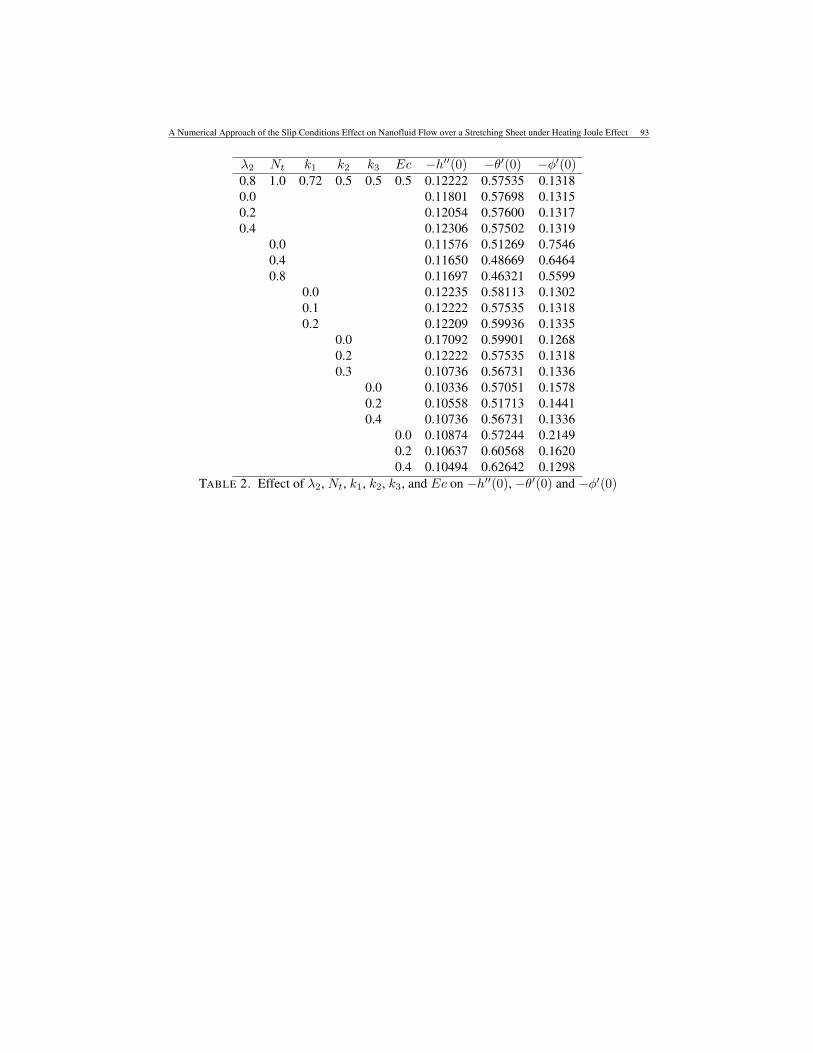
This increment is responsible for the increment of the thickness of the thermal boundarylayer. Figure 17 is plotted for the temperature profile with the use of different values for theheat sink parameter. If we increase the values of the heat sink, then the temperature profiledecreases. This implies that it removes heat from the sheet which decreases thickness of theboundary layer. Figure 18 represents the concentration profile by using different values forthe heat source parameter. If we step up the value of the heat source, then the concentrationprofile decreases. Figure 19 is plotted for the concentration profile with the use of differentvalues for the heat sink parameter. If we increase the value of the heat sink then concentra-tion profile increases. Table 1–2 is prepared for the influence of various parameters on skinfriction Cf , Nusselt numberNux and Sherwood numbers Sh. Table 1 shows that heat skinfriction increases with an increase in M , A, Pr, δ, Le and λ1. The skin friction steps upby the incrementing values of Nb. Nux increases with an increase in M , δ, and Le. Nuxsteps down by increasing values of Pr, A, Le and λ1. Sherwood number Shx increasesby the incrementing values of A, Pr, Nb, and λ1. Sherwood number Shx is reduced byincreasing values of M , δ and Le. The Table 2 shows that the skin friction steps up byincrementing the values of λ2, Nt, k1 and k3. Skin friction increments by the incrementingthe values of k2. Nux increases with an increase in λ2, Nt k2 and Ec. Nux reduces byincreasing values of k1 and k3. Sherwood number Shx steps up with an increment in k1
and k3. Sherwood number Shx decreases by increasing values of λ2, Nt, k2 and Ec.
5. CONCLUSIONS AND FUTURE WORK
The present work is the analysis of an unsteady incompressible magnetohydrodynamicsboundary layer flow heat transfer and a nanofluid over a stretching sheet under the effectof slip boundary conditions and heating joule in the existence of heat source or sink hasbeen considered. We use similarity transformation for transforming the nonlinear coupledordinary differential equations. We successfully computed the solution of coupled ordinarydifferential equations via numerical scheme through shooting method followed by Runge-Kutta Fehlberg method. The behaviour of various parameters on velocity, temperature and
88 Hafiz Abdul Wahab, Hussan Zeb, Saira Bhatti, Muhammad Gulistan and Sarfaraz Ahmad
0 1 2 3 4 5 6 70
0.1
0.2
0.3
0.4
0.5
0.6
0.7
0.8
h′ (η)
η
M=0.0M=0.3M=0.6M=1.0
Nt=0.3; Pr=0.74; Nb=0.2; A=0.3;Le=0.6; Ec=0.1; k2=0.3; k1=0.3; λ=0.1; δ=0.3;λ1=0.2; k3=0.2. λ2=0.2.
0 1 2 3 4 5 6 70
0.1
0.2
0.3
0.4
0.5
0.6
0.7
0.8
θ(η)
η
M=0.0M=0.3M=0.6M=1.0
Nt=0.3; Pr=0.74; Nb=0.2;Le=0.6; Ec=0.1; k2=0.3; k1=0.3; λ=0.1; δ=0.3;A=0.3,λ1=0.2; k3=0.2. λ2=0.2.
FIGURE 3. The variation of h′ and θ for distinct values of M .
0 1 2 3 4 5 6 70
0.1
0.2
0.3
0.4
0.5
0.6
0.7
0.8
0.9
φ(η)
η
M=0.0M=0.3M=0.6M=0.9
Nt=0.2; Pr=0.72; Nb=0.2; A=0.2; Le=0.4; Ec=0.5; k1=0.3;δ=0.3;λ1=0.2; k3=0.2.λ2=0.2; k2=0.3;
0 1 2 3 4 50
0.1
0.2
0.3
0.4
0.5
0.6
0.7
0.8
0.9
φ(η)
η
A=0.0A=0.3A=0.6A=0.9
Nt=0.2; Pr=0.72; Nb=0.3; A=1.0;M=0.1; Le=0.3; Ec=0.1; k2=0.3; k1=0.3; λ=0.1;δ=0.3; λ1=0.2; k3=0.2.λ2=0.2;
FIGURE 4. The variation of φ for distinct values of M and A.
0 1 2 3 4 5 6 70
0.1
0.2
0.3
0.4
0.5
0.6
0.7
0.8
θ(η)
η
Pr=0.64Pr=0.8Pr=1.0Pr=1.3
Nt=0.3; Pr=1.3; Nb=0.2; A=0.3; M=0.3; Le=0.6; Ec=0.1; k2=0.3; k1=0.3; λ=0.1;δ=0.3; λ1=0.2; k3=0.2.λ2=0.2;
0 1 2 3 4 5 6 70
0.1
0.2
0.3
0.4
0.5
0.6
0.7
0.8
φ(η)
η
Pr=0.6Pr=0.8Pr=1.0Pr=1.3
Nt=0.3; Pr=1.3; Nb=0.2; A=0.3;M=0.3; Le=0.6; Ec=0.1; k2=0.3;k1=0.3; λ=0.1;δ=0.3;λ1=0.2; k3=0.2.λ2=0.2;
FIGURE 5. The variation of θ and φ for distinct values of Pr.
A Numerical Approach of the Slip Conditions Effect on Nanofluid Flow over a Stretching Sheet under Heating Joule Effect 89
0 1 2 3 4 5 6 70
0.1
0.2
0.3
0.4
0.5
0.6
0.7
0.8h′ (η
)
η
λ1=0.0λ1=0.3λ1=0.6λ1=0.9
Nt=0.2; Pr=0.72; Nb=0.3;A=0.3; M=0.1; Le=0.6; k2=0.3;k1=0.3;δ=0.3;λ1=0.2; k3=0.2, Ec=0.1;
0 1 2 3 4 5 6 70
0.1
0.2
0.3
0.4
0.5
0.6
0.7
0.8
0.9
θ(η)
η
λ1=0.0λ1=0.4λ1=0.8λ1=1.2
Nt=0.8; Pr=0.72; Nb=0.8; M=0.3; Le=0.3; Ec=0.2; k1=0.3;δ=0.3;A=0.2; k3=0.2.λ2=0.2; k2=0.3;
FIGURE 6. The variation of h′ and θ for distinct values of λ1.
0 1 2 3 4 5 6 70
0.1
0.2
0.3
0.4
0.5
0.6
0.7
0.8
h′ (η)
η
λ2=0.0λ2=0.3λ2=0.6λ2=0.9
Nt=0.2; Pr=0.72; Nb=0.3;A=0.3; M=0.1; Le=0.6; k2=0.3;k1=0.3;δ=0.3;λ1=0.2; k3=0.2, Ec=0.1;
0 1 2 3 4 5 6 7 8 90
0.1
0.2
0.3
0.4
0.5
0.6
0.7
0.8
0.9
θ(η)
η
λ2=0.0λ2=0.3λ2=0.6λ2=0.9
Nt=0.2; Pr=0.72; Nb=0.2; A=0.2; M=0.9; Le=0.4; Ec=0.5; k1=0.3;δ=0.3;λ1=0.2; k3=0.2.λ2=0.2; k2=0.3;
FIGURE 7. The variation of h′ and θ for distinct values of λ2
0 1 2 3 4 5 6 70
0.1
0.2
0.3
0.4
0.5
0.6
0.7
0.8
θ(η)
η
Nb=0.4Nb=0.8Nb=1.2Nb=1.6
Nt=0.2; Pr=0.64; A=0.3;M=0.3; Le=0.4; Ec=0.1;k2=0.3;k1=0.3; λ=0.1;δ=0.3;λ1=0.2; k3=0.2.λ2=0.2;
0 1 2 3 4 5 6 70
0.1
0.2
0.3
0.4
0.5
0.6
0.7
0.8
θ(η)
η
Nt=0.0Nt=0.5Nt=1.0Nt=1.5
Pr=0.74; Nb=0.2; A=0.3;M=0.3; Le=0.6; Ec=0.1; k2=0.3;k1=0.3; λ=0.1;δ=0.3;λ1=0.2; k3=0.2.λ2=0.2;
FIGURE 8. The variation of θ for distinct values of Nb and Nt on θ.
concentration profiles are shown graphically. The behaviour of the local skin friction coef-ficient, local Nusselt number and local Sherwood number are shown numerically throughtable. The major conclusions are listed bellow;
90 Hafiz Abdul Wahab, Hussan Zeb, Saira Bhatti, Muhammad Gulistan and Sarfaraz Ahmad
0.85 0.9 0.95 1 1.05 1.10.42
0.44
0.46
0.48
0.5
0.52θ(
η)
η
Ec=0.0Ec=0.5Ec=1.0Ec=1.5
Nt=0.2; Pr=0.72; Nb=0.3; A=0.2;M=0.3; Le=0.3; Ec=1.5; k1=0.3;δ=0.3;λ1=0.2;k3=0.2.λ2=0.2; k2=0.3;
1.95 1.96 1.97 1.98 1.99 20.179
0.18
0.181
0.182
0.183
0.184
0.185
0.186
0.187
0.188
φ(η)
η
Ec=0.0Ec=0.5Ec=1.0Ec=1.5
Nt=0.2; Pr=0.72; Nb=0.2; A=0.2;M=0.2; Le=0.4;k1=0.3;δ=0.3;λ1=0.2;k3=0.2.λ2=0.2; k2=0.3;
FIGURE 9. The variation θ and φ for distinct values of Ec.
0 1 2 3 4 5 6 70
0.1
0.2
0.3
0.4
0.5
0.6
0.7
0.8
0.9
φ(η)
η
Le=0.3Le=0.4Le=0.5Le=0.6
Nt=0.2; Pr=0.72; Nb=0.3; A=1.0; M=0.1; Le=0.3; Ec=0.1; k2=0.3; k1=0.3; λ=0.1;δ=0.3;λ1=0.2; k3=0.2.λ2=0.2;
FIGURE 10. The variationof φ for distinct values ofLe.
0 1 2 3 4 5 6 70
0.1
0.2
0.3
0.4
0.5
0.6
0.7
0.8
φ(η)
η
Nb=0.4Nb=0.8Nb=1.2Nb=1.8
Nt=0.2; Pr=0.64; Nb=1.9; A=0.3;M=0.3; Le=0.4; Ec=0.1;k2=0.3;k1=0.3; λ=0.1;δ=0.3;λ1=0.2; k3=0.2.λ2=0.2;
FIGURE 11. The variationof φ for distinct values ofNb.
0 1 2 3 4 5 6 70
0.1
0.2
0.3
0.4
0.5
0.6
0.7
0.8
0.9
1
φ(η)
η
Nt=0.0Nt=0.3Nt=0.6Nt=0.9
Nt=0.9; Pr=0.74; Nb=0.2; A=0.3;M=0.3; Le=0.6; Ec=0.1; k2=0.3; k1=0.3; λ=0.1;δ=0.3;λ1=0.2; k3=0.2.λ2=0.2;
FIGURE 12. The variationof φ for distinct values ofNt.
0 1 2 3 4 5 6 70
0.1
0.2
0.3
0.4
0.5
0.6
0.7
0.8
0.9
1
h′ (η)
η
k1=0.0k1−0.3k1=0.6k1=0.9
Nt=0.2; Pr=0.72; Nb=0.3;A=0.3;M=0.1; Le=0.6; Ec=0.0;δ=0.3;λ1=0.2;k3=0.2.λ2=0.2; k2=0.3;
FIGURE 13. The variationof h′ for distinct values ofk1.
A Numerical Approach of the Slip Conditions Effect on Nanofluid Flow over a Stretching Sheet under Heating Joule Effect 91
0 1 2 3 4 5 6 70
0.1
0.2
0.3
0.4
0.5
0.6
0.7
0.8
0.9
1
θ(η)
η
k2=0.0k2=0.2k2=0.4k2=0.6
Nt=0.2; Pr=0.72; Nb=0.3; M=0.1; Le=0.6; Ec=0.1; k1=0.3;δ=0.3;λ1=0.2;k3=0.2.λ2=0.2;A=0.3;
FIGURE 14. Influence ofk2 on θ.
0 1 2 3 4 5 6 7 80
0.1
0.2
0.3
0.4
0.5
0.6
0.7
0.8
0.9
1
φ(η)
η
k3=0.0k3=0.2k3=0.4k3=0.6
Nt=0.2; Pr=0.72; Nb=0.3; A=0.3;M=0.1; Le=0.6; Ec=0.0; k1=0.3;δ=0.3;λ1=0.2;λ2=0.2; k2=0.3;
FIGURE 15. The variationof φ for distinct values ofk3.
0 1 2 3 4 5 6 70
0.1
0.2
0.3
0.4
0.5
0.6
0.7
0.8
0.9
θ(η)
η
δ=−0.2δ=0.0δ=0.2δ=0.4
Nt=0.2; Pr=0.72; Nb=0.3; ;M=0.3; Le=0.3; Ec=0.2; k1=0.3;λ1=0.2;A=0.2k3=0.2.λ2=0.2; k2=0.3;
FIGURE 16. The variationof θ for distinct values of δ.
0 1 2 3 4 5 6 70
0.1
0.2
0.3
0.4
0.5
0.6
0.7
0.8
0.9θ(
η)
η
δ=0.0δ=−0.2δ=−0.4δ=−0.6
Nt=0.8; Pr=0.72; Nb=0.8; A=0.2;M=0.3; Le=0.3; Ec=0.2; k1=0.3;λ1=0.2; k3=0.2.λ2=0.2; k2=0.3;
FIGURE 17. The variationof θ for distinct values of δ.
0 1 2 3 4 5 6 70
0.1
0.2
0.3
0.4
0.5
0.6
0.7
0.8
0.9
φ(η)
η
δ=0.0
δ=0.2
δ=0.4
δ=0.6
Nt=0.2; Pr=0.72; Nb=0.2;A=0.2, M=0.2; Le=0.4;Ec=0.2;k1=0.3;λ1=0.2;k3=0.2.λ2=0.2; k2=0.3;
FIGURE 18. The be-haviour of δ on φ.
0 1 2 3 4 5 6 70
0.1
0.2
0.3
0.4
0.5
0.6
0.7
0.8
0.9
φ(η)
η
δ=0.0δ=−0.2δ=−0.4δ=−0.6
Nt=0.8; Pr=0.72; Nb=0.8; A=0.2;M=0.3; Le=0.3; Ec=0.2; k1=0.3;λ1=0.2; k3=0.2.λ2=0.2; k2=0.3;
FIGURE 19. The be-haviour of δ on φ.
92 Hafiz Abdul Wahab, Hussan Zeb, Saira Bhatti, Muhammad Gulistan and Sarfaraz Ahmad
A M Pr δ Le Nb λ1 −h′′(0) −θ′(0) −φ′(0)0.8 1.0 0.72 0.5 0.5 0.5 0.5 0.12222 0.57535 0.13180.0 0.11130 0.48859 0.15430.2 0.11417 0.51136 0.14800.4 0.11695 0.53340 0.1422
0.0 0.10736 0.58869 0.12850.2 0.11053 0.58578 0.12920.4 0.11359 0.58300 0.1299
1.0 0.12099 0.53798 0.14171.3 0.11989 0.50762 0.14951.6 0.11900 0.48595 0.1548
-0.4 0.12480 0.68052 0.1023-0.2 0.12427 0.65881 0.10840.0 0.12372 0.63620 0.11480.2 0.12314 0.61264 0.1214
0.0 0.12247 0.57527 0.12690.2 0.12232 0.57531 0.12990.4 0.12217 0.57537 0.1328
0.2 0.12000 0.61117 0.16380.4 0.12189 0.68796 0.13730.4 0.12241 0.66397 0.1282
0.0 0.13071 0.57135 0.13270.2 0.12730 0.57297 0.13240.4 0.12391 0.57456 0.1320
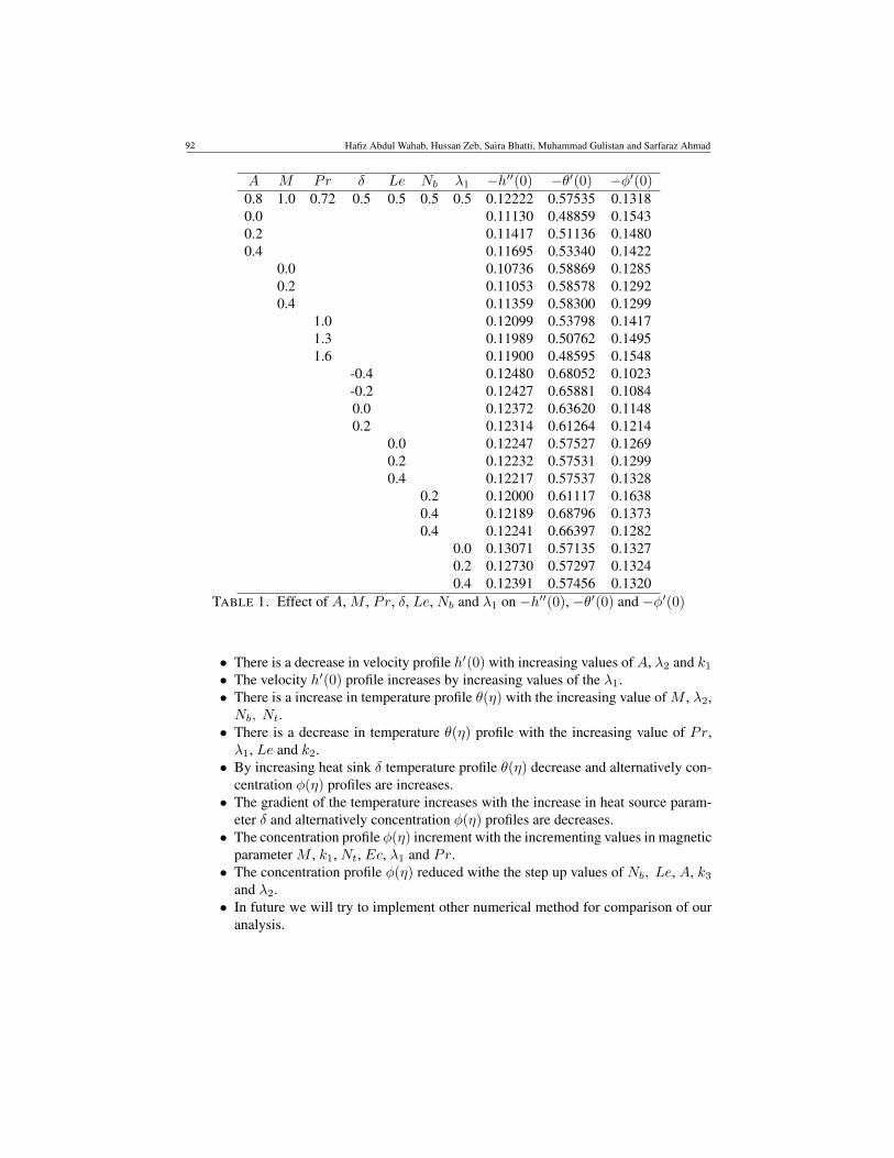
TABLE 1. Effect of A, M , Pr, δ, Le, Nb and λ1 on −h′′(0), −θ′(0) and −φ′(0)
• There is a decrease in velocity profile h′(0) with increasing values of A, λ2 and k1
• The velocity h′(0) profile increases by increasing values of the λ1.• There is a increase in temperature profile θ(η) with the increasing value of M , λ2,Nb, Nt.
• There is a decrease in temperature θ(η) profile with the increasing value of Pr,λ1, Le and k2.
• By increasing heat sink δ temperature profile θ(η) decrease and alternatively con-centration φ(η) profiles are increases.
• The gradient of the temperature increases with the increase in heat source param-eter δ and alternatively concentration φ(η) profiles are decreases.• The concentration profile φ(η) increment with the incrementing values in magnetic
parameter M , k1, Nt, Ec, λ1 and Pr.• The concentration profile φ(η) reduced withe the step up values of Nb, Le, A, k3
and λ2.• In future we will try to implement other numerical method for comparison of our
analysis.
A Numerical Approach of the Slip Conditions Effect on Nanofluid Flow over a Stretching Sheet under Heating Joule Effect 93
λ2 Nt k1 k2 k3 Ec −h′′(0) −θ′(0) −φ′(0)0.8 1.0 0.72 0.5 0.5 0.5 0.12222 0.57535 0.13180.0 0.11801 0.57698 0.13150.2 0.12054 0.57600 0.13170.4 0.12306 0.57502 0.1319
0.0 0.11576 0.51269 0.75460.4 0.11650 0.48669 0.64640.8 0.11697 0.46321 0.5599
0.0 0.12235 0.58113 0.13020.1 0.12222 0.57535 0.13180.2 0.12209 0.59936 0.1335
0.0 0.17092 0.59901 0.12680.2 0.12222 0.57535 0.13180.3 0.10736 0.56731 0.1336
0.0 0.10336 0.57051 0.15780.2 0.10558 0.51713 0.14410.4 0.10736 0.56731 0.1336
0.0 0.10874 0.57244 0.21490.2 0.10637 0.60568 0.16200.4 0.10494 0.62642 0.1298
TABLE 2. Effect of λ2, Nt, k1, k2, k3, and Ec on −h′′(0), −θ′(0) and −φ′(0)
94 Hafiz Abdul Wahab, Hussan Zeb, Saira Bhatti, Muhammad Gulistan and Sarfaraz Ahmad
REFERENCES
[1] K. A. Abro and M. A. Solangi, Heat Transfer in Magnetohydrodynamic Second Grade Fluid with PorousImpacts using Caputo-Fabrizoi Fractional Derivatives, Punjab Univ. j. math. 49, No. 2 (2017) 113–125.
[2] K. A. Abro, M. Hussain and M. M. Baig, A Mathematical Analysis of Magnetohydrodynamic GeneralizedBurger Fluid for Permeable Oscillating Plate, Punjab Univ. J. Math. Vol. 50, No. 2 (2018) 97-111.
[3] S. Abelman, E. Momoniat and T. Hayat, Magnetohydrodynamic Oscillating and Rotating Flows of MaxwellElectrically Conducting Fluids in a Porous Plane, Punjab Univ. j. math. 50, No. 3 (2018) 61–71.
[4] R. Ahmad and Waqar A. Khan, Unsteady heat and mass transfer magnetohydrodynamic (MH) nanofluidflow over a stretching sheet with heat source/sink using quasi-linearization technique, Canadian J. of Phy.93, No. 12 (2015) 1477-1485.
[5] H. Alfve, Existence of electromagnetic hydrodynamic waves, J. Appl. Math. Phys. 150, No. 3805 (1942)405–506.
[6] A. Ali, M. Tahir, R. Safdar, A. U. Awan, M. Imran and M. Javaid, Magnetohydrodynamic Oscillating andRotating Flows of Maxwell Electrically Conducting Fluids in a Porous Plane, Punjab Univ. J. Math. Vol. 50,No. 4 (2018) 61-71.
[7] H. I. Andersson, Slip flow past a stretching surface, Acta Mechanica 158, No. 1–2 (2002) 121–125.[8] A. U. Awan, M. Imran, M. Athar and M. Kamran, Exact analytical solutions for a longitudinal flow of a
fractional Maxwell fluid between two coaxial cylinders, Punjab Univ. j. math. 45, (2013) 9-23.[9] A. U. Awan, R. Safdar, M. Imran and A. Shoukat, Effects of Chemical Reaction on the Unsteady Flow of
an Incompressible Fluid over a Vertical Oscillating Plate, Punjab Univ. j. math. 48, No. 2 (2016) 167-182.[10] N. Bachok, A. Ishak and I. Pop, Boundary-layer flow of nano fluids over a moving surface in moving fluid,
Int. J. Ther. Sci. 48, No. 9 (2010) 1663–1668.[11] Jacopo Buongiorno, and David C. Venerus, A benchmark study on the thermal conductivity of nano fluids,
Journal of Applaid Physics, 106, No. 617 (2009) 094312–0943126.[12] R. Bhargava and M. Goyal. Mhd non-newtonian nano fluid flow over a permeable stretching sheet with heat
generation and velocity slip, Int. Scholarly and Scientific Research and Innovation 8, No. 6 (2008) 909–916.[13] A. S. Bhuiyan, N. H. M. A. Azim and M. K. Chowdhury, Joule heating effects on MHD natural convection
flows in presence of pressure stress work and viscous dissipation from a horizontal circular cylinder, J. Appl.Fluid Mech. 7, No. 1 (2014) 7–13.
[14] J. L. Crane, Flow past a Stretching Plate, ZAMP. 21, No. 4 (1970) 645-647.[15] H. M. Duwairi, Fin placement for optimal forced convection heat transfer from a cylinder in cross flow, Int.
J. Numerical Methods for Heat and Fluid Flow 15, No. 3 (2005) 277 – 295.[16] M. Govindaraju and N. V. Ganesh, Entropy generation analysis of magneto hydrodynamic flow of a nano
fluid over a stretching sheet, J. Egyptian Math. Soc. 23, No. 2 (2015) 429–434.[17] W. Ibrahim and B. Shankar, MHD boundary layer flow and heat transfer of a nano fluid past a permeable
stretching sheet with velocity thermal and solutal slip boundary conditions, Computers and Fluids 75, (2013)1–10.
[18] M. Ishaq, G. Ali, S. I. A. Shah, Z. Shah, S.r Muhammad and S. A. Hussain, Nanofluid Film Flow of EyringPowell Fluid with Magneto Hydrodynamic Effect on Unsteady Porous Stretching Sheet, Punjab Univ. J.Math. Vol. 51, No. 3 (2019) 147-169.
[19] H. Hua and X. Su. Unsteady mhd boundary layer flow and heat transfer over the stretching sheets submergedin a moving fluid with ohmic heating and frictional heating, Open Phy. 13, No. 1 (2015) 210–217.
[20] S. A. Hussain, G. Ali, S. I. A. Shah, S. Muhammad and M. Ishaq, Bioconvection Model for Magneto Hydro-dynamics Squeezing Nanofluid Flow with Heat and Mass Transfer Between Two Parallel Plates ContainingGyrotactic Microorganisms Under the Influence of Thermal Radiations, Punjab Univ. J. Math. Vol. 51, No.4 (2019) 13-36.
[21] K. Karimi and A. Bahadorimrhr, Rational Bernstein Collocation Method for Solving the Steady Flow of aThird GradeFluid in a Porous Half Space, Punjab Univ. j. math. 49, No. 1 (2017) 63-73.
[22] M. Y. Malik, I. Khan, A. Hussain and T. Salahuddin, Mixed convection flow of MHD Eyring powell nanofluid over a stretching sheet a numerical study, AIP Advance 5, No. 11 (2015), 117118–117121.
[23] M. Y. Malik and T. Salahuddin, Numerical solution of MHD stagnation point flow of williamson fluid modelover a stretching cylinder, Int. J. Nonlinear Sci. 16, No. 3 (2015) 161–164.
A Numerical Approach of the Slip Conditions Effect on Nanofluid Flow over a Stretching Sheet under Heating Joule Effect 95
[24] S. Mansur and A. Ishak, The magnetohydrodynamic boundary layer flow of a nano-fluid past a stretch-ing/shrinking sheet with slip boundary conditions, J. Appl. Math. (2014) 181–188.
[25] S. Mukhopadhyay, MHD boundary layer flow and heat transfer over an exponentially stretching sheet em-bedded in a thermally stratified medium, Alex. Eng. J. 52, No. 3 (2013) 259–265.
[26] S. Nadeem, R. Mehmood and N. S. Akbar, Non-orthogonal stagnation point flow of a nano nonNewtonianfluid towards a stretching surface with heat transfer, Int. J. Heat and Mass Transfer 57, No. 2 (2013) 679–689.
[27] M. K. Partha, P. V. S. N. Murthy and G. P. Rajasekhar, Effect of viscous dissipation on the mixed convectionheat transfer from an exponentially stretching surface, Heat Mass Transfer 41, No. 4 (2005) 360–366.
[28] T. Poornima and N. Bhaskar, Radiation effects on MHD free convective boundary layer flow of nano fluidsover a nonlinear stretching sheet. advances in applied science research, Adv. Appl. Sci. Res. 4, No. 2 (2013)190–202.
[29] M. G. Reddy, Thermal radiation and chemical reaction effects on steady convective slip flow with uniformheat and mass flux in the presence of ohmic heating and a heat source, J. Appl. Fluid Mech. 10, No. 4 (2014)417–442.
[30] K. V. S. Raju, T. Sudhakar Reddy, M. C. Raju, P. V. Satya Narayana and S. Venkataramana, MHD convectiveflow through porous medium in a horizontal channel with insulated and impermeable bottom wall in thepresence of viscous dissipation and joule heating, Ain. Shams Eng. J. 5, No. 2 (2013) 543–551.
[31] N. Raza, Unsteady Rotational Flow of a Second Grade Fluid with Non-Integer Caputo Time FractionalDerivative, Punjab Univ. J. Math. Vol. 49, No. 3 (2017) 15-25.
[32] R. Safdar, M. Imran, M. Tahir, N. Sadiq and M. A. Imran, MHD Flow of Burgers Fluid under the Effect ofPressure Gradient Through a Porous Material Pipe, Punjab Univ. j. math. 50, No. 4 (2018) 73-90.
[33] N. Sadiq, M. Imran, R. Safdar, M. Tahir and M Javai, Exact Solution for Some Rotational Motions ofFractional Oldroyd-B Fluids Between Circular Cylinders, Punjab Univ. J. Math. 50, No. 4 (2018) 39-59.
[34] B. C. Sakiadis, Boundary layer behaviour on continuous solid surface,ii. the boundary layer on a continuousat surface, J. Am. Inst. Chem. Eng. 7, No. 2 (1969) 221–225.
[35] V. P. Shidlovskiy, Introduction to the dynamics of rarefiled gases, American Elsevier Publishing (1967).[36] J. Vleggaar, Laminar boundary layer behaviour on continuous accelerating surface, Chem. Eng. Sci., 32,
No. 12 (1977) 1517–1525.[37] Yoshimura and R. K. Prud, Wall slip corrections for couette and parallel disk viscometry, J. Rheo. 32, No.
53 (1988) 53–67.[38] A. A. Zafar, M. B. Riaz and M. A. Imran, Unsteady Rotational Flow of Fractional Maxwell Fluid in a
Cylinder Subject to Shear Stress on the Boundary, Punjab Univ. J. Math. Vol. 50, No. 2 (2018). 21-32.[39] H. Zeb, H. A Wahab, M. Shahzad, S. Bhatti and M. Gulistan, Thermal effects on MHD unsteady Newtonian
fluid flow over a stretching sheet, J. of Nano fluids. 7, No. 5 (2018) 704–710.[40] H. Zeb, H. A Wahab, M. Shahzad, S. Bhatti and M. Gulistan, A numerical approach for the thermal radiation
on MHD unsteady Newtonian fluid flow over a stretching sheet with variable thermal conductivity and partialslip conditions, J. of Nano fluids. 7, No. 5 (2018) 870–878.