Purchasing power parity and Austria's exchange rate ... · Purchasing power parity and Austria's exchange rate strategy: some empirical evidence of their relationship Christine Gartner

Purchasing power parity and Austria's exchange rate strategy: some empirical evidence of their relationship

Christine Gartner and Heinz Glück1

Introduction

In the concept of Austria's exchange rate policy, the pegging to stable currencies of important trading partners is regarded as an intermediate target in order to maintain low inflation and to improve competitiveness. In the longer view, the credible implementation of a policy like this will stabilise expectations and reduce uncertainties. What is crucial in this context is the development of the real exchange rate. There exists, as is well known, a close link between the evolution and the time-series properties of a country's real exchange rate and the concept of purchasing power parity (PPP). However, in the 1970s and 1980s most empirical studies rejected the validity of this concept. Consequently, in the course of the evolution of Austria's exchange rate policy, PPP was never regarded as an essential element nor as a source of potential contradiction to actual policy.

Recent years, however, have seen a new and increasing interest in PPP. This revival may among other things, have two reasons: First, the relative simplicity and intuitive clarity of this concept, and, second, the development of new econometric methods, especially time-series analysis, which offered new tests to evaluate the validity of PPP. The results, however, are still quite tentative, but generally point to the fact that at least in the very long run PPP probably cannot be rejected (see, for instance, Kim 1990).

Thus, the purpose of this paper is twofold: First, as there are very few studies using Austrian data, we look at the time-series properties of the schilling's real effective exchange rate in the light of these new developments. As will be shown, the results are not supportive for PPP; therefore, in a second step, we try to identify other (or additional) factors which may influence the evolution of the real exchange rate.

We proceed as follows: In Section 1 the Austrian exchange rate policy and its relation to PPP are reviewed. Section 2 discusses some recent research on PPP, and in Section 3 we present the empirical results for Austria on the real effective exchange rate. The last section concludes the paper.

1. Austria's exchange rate policy and the Schilling's real effective exchange rate

There are various articles on Austria's exchange rate policy (Gartner 1995, Glück, Proske and Tatom 1992, Glück 1994, Gnan 1995, Hochreiter and Winckler 1995, Pech 1994, and others). In a nutshell, this policy and its evolution can be summarised as follows:

Since the end of World War II, Austria has consistently followed a policy of fixing the exchange rate of the Austrian schilling. First, during the Bretton Woods era the schilling was fixed to the US $ between 1953 (unification of the exchange rate) and August 1971. During this time there was only one parity change, namely a revaluation of the schilling against the US$ by 5.05% in May 1971. Second, when the United States closed the gold window in August 1971, Austria's exchange rate policy had to be adapted. A free float was not considered feasible by the Austrian authorities because of the exchange rate uncertainties connected with it and because of a perceived underlying speculative

1 The views expressed in this paper are those of the authors, not necessarily of the institution they are affiliated with. We are grateful for valuable comments by Palle Andersen and Peter Brandner. Any mistakes, of course, remain ours.

- 6 3 -

threat due to the lack of market depth and width which might threaten the stability of the currency and the economy. Instead, Austria pioneered a new concept by pegging its exchange rate against a basket of currencies. In the following period, the composition of the basket in terms of currencies and base dates was frequently adjusted. As the importance of the DM as reference currency rose, a peg exclusively to this currency emerged in the second half of the 1970s. Finally, since the end of 1981 the schilling has remained fixed to the DM with practically no fluctuation margin.

What is particularly interesting with regard to Austria's economic policy in general and exchange rate policy in particular is that the authorities in the 1970s (specifically related to the evolution of the schilling with regard to the DM in May 1974) explicitly accepted a real appreciation of the schilling in order to get domestic inflation on a lower path. At the same time, it was recognised that this policy could entail considerable costs, in particular for the exposed sector of the economy. Hence, it was attempted to mitigate the initial costs of the real appreciation by an expansionary fiscal policy and, to some extent, also through temporary subsidies. However, the authorities were confident that over the longer term the economy would benefit because wage pressures would be reduced in the wake of lower inflation; consequently profit margins and employment could be restored.

It is important to note that Austria's specific institutional framework, i.e. the social partnership, has a significant role to play in order to ensure that wage developments are commensurate with productivity increases and that economic policy is designed in such a way as to be conducive to an improvement of the supply-side and to foster general economic flexibility. Sound fiscal policy, innovative supply side policies and an institutional framework enhancing the overall flexibility of the economy go far towards explaining the success of Austria's virtually fixed single currency peg against a stable anchor currency in the face of occasional shocks, even of severe real asymmetric shocks.

In short, the concept of the hard-currency option can be described as follows:

• It provides the possibility of importing stability via the pass-through from the prices of imported goods to consumer prices or to the prices of production inputs.

• The tough performance of the currency causes a profit squeeze in the exposed sector which leads to rationalisation, innovation, rising productivity, and improved structures. It also prevents excessive wage increases in this sector which keeps the wage level low in the sheltered sector, too.

• By these mechanisms - lower inflation rates as a precondition for a moderate incomes policy and a profit squeeze in the exposed sector leading to structural improvements - "virtuous circle" effects are brought into play.

Assuming PPP, this can simply be interpreted in the following way (Handler 1989): In relation to the anchor country, diverging price developments are not used as explanatory variable for the exchange rate but as an equilibrium condition by means of which the domestic price level (p) is determined:

p = p* + s2

with s = log of nominal exchange rate

p = log of domestic price level

p* = log of foreign price level,

By fixing the exchange rate to the anchor country's currency, i.e. 5 = 0, stability from this country is imported, and the implicit inflation target is defined as,p=p*.

This, of course, implies also a constant real exchange rate vis-à-vis the anchor country. If, on the other hand, the anchor country's inflation rate is the goal which is aimed for, but which - as

2 Relations of this kind have been tested empirically by Ardeni and Lubian (1991).

- 6 4 -

was frequently the case for Austria vis-à-vis Germany - cannot be attained, i.e. p tends to be higher than p*, this would imply a continuous real appreciation of the pegging country's currency.

The case is different when we look at the pegger's exchange rate vis-à-vis the weighted average of exchange rates of its trading partners, i.e. the nominal effective exchange rate. As the exchange rate of the average Austrian trading partner tended to be weaker than the DM and the schilling, a nominal revaluation of the latter was the effect. As, on the other hand, inflation rates in Germany (and in Austria) were lower than for the trading partners, the real effective revaluation generally was smaller than the nominal one, or, in the ideal case, even a real effective devaluation could be the outcome, a favourable effect for international competitiveness.

It is characteristic for Austria's exchange rate policy that over the course of the years it has been developing in a rather pragmatic way which sometimes was in contradiction to textbook wisdom. Similarly, there has been no concern about mean-reverting by which - after a shock -nominal and real exchange rates would be forced back to equilibrium levels as determined by PPP. On the contrary, there was (and is) much more the intuitive belief that by the very absence of mean-reversion exchange rates could be used in order to achieve specific economic goals even in the long run. In the following we try to investigate whether recently developed tests applied to Austrian data justify this view.

2. Tests of PPP and time series analysis

Most recent literature describes the idea of long-run PPP as the hypothesis that there exists a stationary equilibrium real exchange rate. Before the virtual explosion of PPP tests that followed the introduction of econometric techniques designed to handle non-stationary data, it had become more or less a stylised fact that PPP was rejected in empirical tests. Since the concepts of integration and cointegration became common knowledge, a large number of empirical tests have been presented. Alexius (1995) gives an overview of the empirical literature on PPP and finds that the results are mixed, so that no final verdict has been reached concerning the validity of the PPP doctrine. She argues that while there is widespread agreement that PPP does not hold in the short run, the disagreement basically concerns the question whether it holds in the long run and how long the long run is. She also finds that a rejection of PPP depends partly on the choice of countries, the length of the sample period and the econometric techniques used. Studies covering less than 15 years of data almost always reject PPP, while those covering a entire century usually do not3. Furthermore, rejections of the PPP hypothesis are much more frequent for the United States and Canada than for European countries. Since most tests of PPP have focused on bilateral exchange rates between major industrial nations like USA, Japan and Germany, a case can be made that these countries have rather different economic structures and the real exchange rate between them is less likely to be stationary than the real exchange rates between more homogenous European countries.

There are two popular approaches testing the validity of PPP. One approach has been to investigate whether the real exchange rates contain a unit root, which is incompatible with PPP. The existence of a unit root in the real exchange rate would imply that shocks to the real exchange rate have not only temporary, but permanent effects: If the real exchange rate is pushed below (above) its equilibrium level, it cannot be expected to return.

The second approach has been to investigate whether nominal exchange rates and price levels are cointegrated. Studies using cointegration techniques have quite often found cointegration among nominal exchange rates and price levels. But the existence of a stationary linear combination of exchange rates and prices does not necessarily mean that PPP holds. According to PPP, it is the

3 Alexius (1995), p.8.

- 6 5 -

real exchange rate that should be stationary. This implies certain restrictions on the cointegration vector(s).

Bilateral PPP has been tested much more often than multilateral PPP. Possible reasons could be that the choice of weights is rather arbitrary and that the hypothesis of stationary effective real exchange rates is not testable within multivariate systems of price levels and bilateral exchange rates.

3. Modelling the long-run real exchange rate for Austria: empirical results

This section presents our empirical findings on determinants of the real exchange rate of the Austrian schilling. Following the line of other recent empirical studies on long-run exchange rate modelling, we will make use of time-series analysis, especially cointegration and unit root testing. In a first step we are interested in knowing whether the PPP doctrine is valid for Austrian data. This seems particularly appealing since the Austrian case is hardly included in the various papers testing PPP. Furthermore, we will concentrate on the examination of the real effective exchange rate, whereas the great bulk of former PPP tests have focused on bilateral real exchange rates. The paper by Johansen and Juselius (1992) and the one by Alexius (1995) represent exceptions to this rule. In agreement with Alexius (1995) we are convinced that if the mechanism driving PPP has to do with international competitiveness, it may be more relevant to study multilateral than bilateral PPP.

In a second step we investigate if real interest rate differences contribute to the modelling of the long-run real exchange rate. However, with a fixed exchange rate regime as in the Austrian monetary policy concept, it seems more appropriate to test the reaction function of the Austrian national bank in which the short-term interest rate is the dependent variable. The test results show that the real interest rate difference is not important for the determination of the real effective exchange rate.

In a third step we look for other determinants of the real effective exchange rate than its own past development. The long-term interest rate difference between Austrian and German government bonds and the productivity differential between the two countries' industrial sectors are regarded as promising candidates.

3.1 Alternative tests of PPP

As mentioned in Section 2 there a two alternative approaches to investigating the validity of PPP. In our empirical examination we made use of both of them.

3.1.1 PPP and cointegration

First, we test the following equation:

J / ^ ß + O o f l + a i # *+<!>, (1)

An informal way to get a first impression of the characteristics of a time series is to inspect the plots of a variable in levels and differences. We show the time plots for the three series in the Figures 1 to 3. As one would expect, all variables show a trending behaviour in the levels. That means that once there is a level change in these series, it remains for a longer time span. The differences of the series appear to be stationary around zero or a constant. This shape indicates the presence of a difference-stationary data generating process. However, it is difficult to distinguish between a trend-stationary and a difference-stationary process by means of time plots of finite sample length. Other and more formal tools exist for this purpose. Since the variables contained in this equation are likely to be nonstationary, our tests like most tests by other authors, have concentrated on exploiting the cointegration methods proposed by Engle and Granger (1987).

- 6 6 -

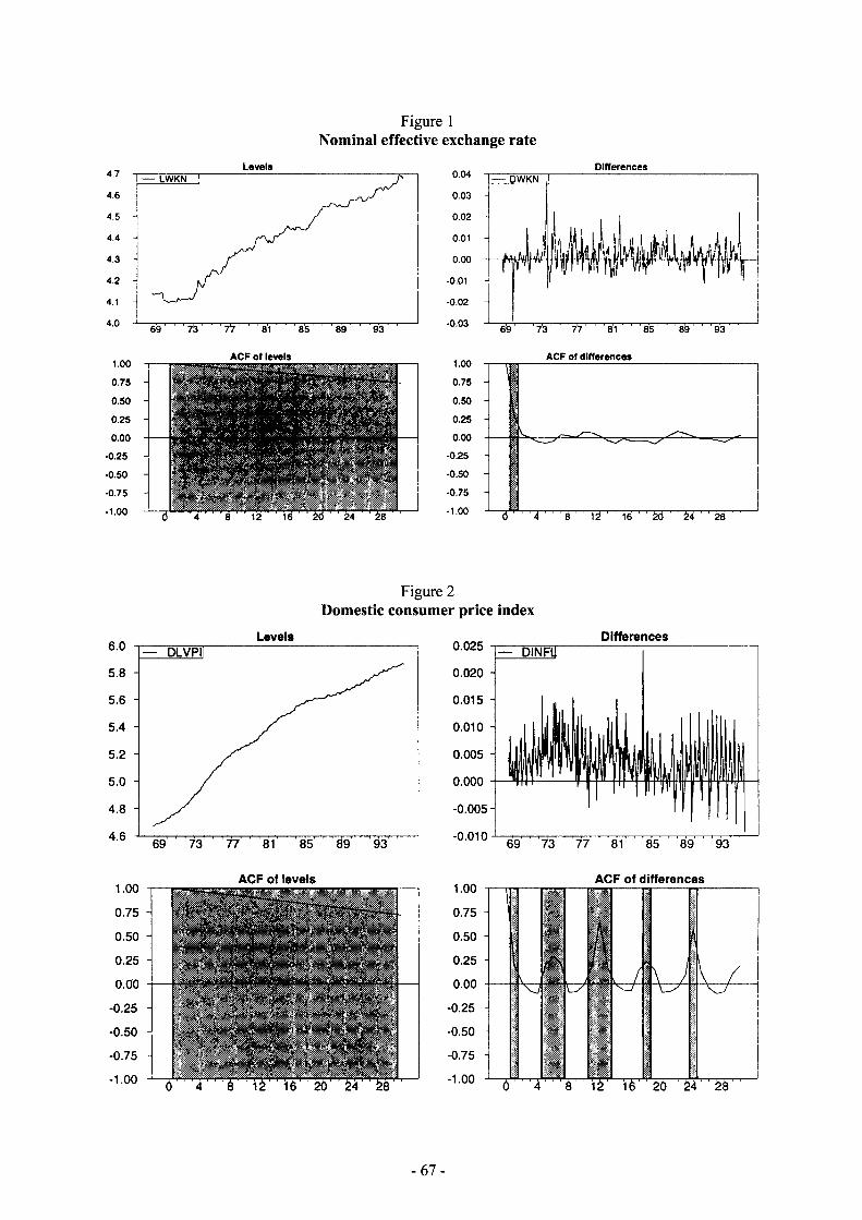
Figure 1 Nominal effective exchange rate

Levels

ACF of levels

4.7

4.6 1 — LWKN 1

1 i

0.04

0.03

4.5 i

i 0.02

4.4 -i I

0.01

4.3

J K / 1 r

0.00

4.2 J K / 1 r -0.01

4.1 ] ̂ — ' -0.02

4.0 ! -0.03 4.0 69 ' ' ' 7'3 ' IT SI ' ' 8 5 ' ' 89 ' 9 3 ' ' -0.03

^ " Í6 20 V r 2 4

Differences

1.00

0.75

0.50

0.25

0.00

•0.25

•0.50

-0.75

-1.00

DWKN

69 ' ' ' 73 ' ' ' f l ' ' ' 81 ' ' ' 8 5 ' ' S9 ' ' ' 93 '

ACF of differences

ó '4 l à ' ' 16 ' ' èd ' ' ¿4 ' ' 28

Figure 2 Domestic consumer price index

Levels

5.0 -

77 81 85

ACF of levels

0.75 -

r * " f i » • * ^

Differences 0.025 — DINFÜ 0.020

0.015

0.010

0.005 -

0.000

0.005

0.010

1.00

0.75

0.50

0.25

0.00

-0.25 -I -0.50

-0.75

- 1 . 0 0

77 81 85 89 93

ACF of differences

iW-A

Ó 4 8 12 i è ¿0 ' 24 ' 28

- 6 7 -

Figure 3 Foreign consumer price index

6.00

5.75

5.50

5.25 -

5.00 -

4.75 -

4.50 -

4.25

Levels FLVPl!

¿9' ' i Z ' t ! ' 01'

1.00

0.75

0.50

0.25

0.00

-0.25

-0.50

-0.75

-1.00

85 89 9 3

ACF of levels

Û 4 '' ' 8 12 16 20 24 ' 28

«fuíZr* <

Differences 0.020 Fl NFL!

0.015

0.010

0.005

0.000

-0.005 -

-0.010

1.00

0.75

0.50

0.25 H

0.00

-0.25 -I -0.50

-0.75

-1.00

69' ' 73 ' ' 'tr' ' 81' ' '£¡5' ' 89

ACF of differences

x

4 ' 8 12 ' 16 ' ' 20 24 ' 28

We used monthly, seasonally unadjusted data of the Austrian nominal effective exchange rate, the Austrian CPI and the so-called "foreign CPI" (which is a basket of trade-share weighted consumer price indices of trading partner countries). To specify the test correctly, we first had to check whether all variables entering the above equation were integrated of order one, 1(1). We tested the stationarity properties of the variables by means of rather informal visual inspection and more formal unit root tests, i.e. the augmented Dickey-Fuller test.

Analysing the autocorrelation function of the levels, the differences and the residuals of a regression against a time trend should reveal more information about whether the time series belong to one of the two model classes. We found that the autocorrelation functions of the levels start at a value of around 0.9 and die out very slowly. In contrast to the levels, the autocorrelation functions of the differences die out quickly, with the exception of the domestic consumer price index, which shows some significant autoregressive components at 6 and 12 lags and multiples of these lags, indicating a seasonal pattern. Since we wanted to avoid the shortcomings induced by seasonal filtering of the time series and also wanted to treat all series alike (we did not find any seasonal pattern in the other variables), we refrained from any of the popular seasonal adjustment transformations.

A third step towards differentiating between trend-stationary and difference-stationary representations of macroeconomic time series could be the calculation of residuals from a regression of the variables against a constant and a linear time trend. Uri and Wehinger (1990) pointed out that the distinction between the individual models is difficult, so it was necessary to carry out some formal tests.

We used the econometric software package RATS (version 4.2) to compute the Dickey-Fuller test statistics, after having specified the number of autoregressive correction terms (arcorrs) p by inspection of the series' ACF. We chose the number of autoregressive correction terms as small as

- 6 8 -

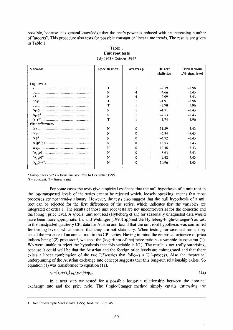
possible, because it is general knowledge that the test's power is reduced with an increasing number of "arcorrs". This procedure also tests for possible constant or linear time trends. The results are given in Table 1.

Table 1 Unit root tests

July 1968 - October 1995*

Variable Specification Arcorrs p DF test Critical value statistics 1 % sign, level

Log-levels s T 1 »2.79 -3.96 P N 4 -4.66 -3.43 P* N 4 -2.99 -3.43 P*/P T 1 -1.91 -3.96 q T 1 -2.70 -3.96 A12P N 1 -1.71 -3.43 A12P* N 1 -2.53 -3.43 (r-r*) T 1 -3.74 -3.96

First differences A s N 0 -11.29 -3.43 A p N 0 -6.34 -3.43 A p* N 0 ^1.72 - 3 4 3 A(p*/p) N 0 -13.73 -3.43 A q N 0 -12.48 -3.43 (A12p) N 0 -8.63 -3.43 (A12p)* N 0 -9.42 -3.43 A12(r-r*) N 0 -10.96 -3.43

* Sample for (r-r*) is from January 1980 to December 1995. N = constant; T = linear trend.

For some cases the tests give empirical evidence that the null hypothesis of a unit root in the log-transposed levels of the series cannot be rejected which, loosely speaking, means that most processes are not trend-stationary. However, the tests also suggest that the null hypothesis of a unit root can be rejected for the first differences of the series, which indicates that the variables are integrated of order 1. The results of those unit root tests are not uncontroversial for the domestic and the foreign price level. A special unit root test (Hylleberg et al.) for seasonally unadjusted data would have been more appropriate. Uri and Wehinger (1990) applied the Hylleberg-Engle-Granger-Yoo test to the unadjusted quarterly CPI data for Austria and found that the unit root hypothesis was confirmed for the log-levels, which means that they are not stationary. When testing for seasonal roots, they stated the presence of an annual root in the CPI series. Having in mind the empirical evidence of price indices being I(2)-processes4, we used the (logarithm of the) price ratio as a variable in equation (1). We were unable to reject the hypothesis that this variable is 1(1). The result is not really surprising, because it could well be that the Austrian and the foreign price levels are cointegrated and that there exists a linear combination of the two I(2)-series that follows a I(l)-process. Also the theoretical underpinning of the Austrian exchange rate concept suggests that this long-run relationship exists. So equation (1) was transformed to equation (la).

^=ßo+a2(A/A*)+<Poi ( l a )

In a next step we tested for a possible long-run relationship between the nominal exchange rate and the price ratio. The Engle-Granger method simply entails estimating the

4 See for example MacDonald (1995), footnote 17, p. 453

- 6 9 -

coefficients of equation (la) by OLS and subjecting the residuals to a variety of diagnostic tests of which the most popular has proven to be the augmented Dickey-Fuller test. If there is no long-run relationship between the variables, the residual series of the cointegrating equation would be nonstationary. If there is a long-run relationship as the traditional PPP doctrine would suggest, then, despite the variables entering the equation being individually nonstationary, there would exist some linear combination that transforms the residuals to an 1(0) series.

The augmented Dickey-Fuller test of the residuals amounts to estimating an equation of the form:

p

A q ^ v j c p ^ + v,-^ A<pf_,.+1 + e, (2) i = 2

If the null hypothesis of no cointegration is valid - the residuals are 1(1) - then Vi should be insignificantly different from 0, and this may be tested using a t-test, denoted T. Under the alternative hypothesis of stationarity, Vj is expected to be significantly negative. As the distribution of X is not standard, Engle-Granger have tabulated the appropriate critical values. Our empirical results refer to the critical values by Engle and Yoo (1987). The paper tabulates critical values for T from a cointegrating regression of up to five variables and for smaller samples. The initial paper by Engle and Granger (1987) only computed critical values for % for an equation with two variables and samples of more than 100 observations.

Table 2a Cointegrating regression of equation (la):

•Sf = ßo + a 2(A/A*) + ( Pof

Variable Coefflcient Standard error t-statistics

/

ft 4.62 0.004 1,250.18 Po

1,250.18

f

cc2 1.65 0.022 76.33

Estimation by Ordinary Least Squares; monthly data from 68:07 to 95:12; usable observations: 330. Degrees of freedom: 328; R2 = 0.95; Durbin-Watson statistic = 0.048.

Table 2b Unit root tests of residuals ((p0i )

Variable Arcorrs p DF test statistics

Critical value* 1% sign, level

9(., 4 -1.57 -3.78

* Engle and Yoo (1987), p. 158. Number of variables in regression (N) = 2.

- 7 0 -

In the context of the cointegration literature, the existence of long-run PPP amounts to satisfying three conditions. Besides the stationarity of the errors, (Pt, of the cointegrating regression5, MacDonald (1995) also mentions the condition of symmetry and the condition of proportionality. The condition of symmetry means that the «o and OCi coefficients in equation (1) should enter the cointegration equation with an (equal and) opposite sign. The condition of proportionality means that both coefficient should equal plus and minus unity. A reformulation of the last two conditions for equation (la) amounts to the requirement that «2 equals 1.

As expected, we did not find empirical evidence of (absolute or relative) PPP holding for Austria. The first and most important condition, namely the stationarity of the residuals of the cointegrating equation (la), could not be confirmed (Table 2a). The results of the unit root test are presented in Table 2b. The estimation results also reject the validity of the two other conditions.6

3.1.2 A random-walk real exchange rate model

As mentioned in Section 2 there is an alternative to testing for cointegration between a nominal exchange rate and relative prices, and examining the PPP theorem. This approach tests the null hypothesis that the real exchange rate follows a random walk against the alternative that PPP holds in the long run. In contrast to the test applied above, these tests impose - rather than test - the hypothesis that a ^ l and test - rather than impose - that the (log of the) real exchange rate (q) is stationary7.

In more technical terms, the test checks the null hypothesis of a random walk (equation 4) against the alternative of a trend-stationary process (equation 5):

¿Sqt = a + co, (4)

where A is the first difference operator, a is a drift term, which captures, perhaps, the failure of real

interest rates to be equalised across countries and CO, is a stationary process.

The alternative hypothesis to the above equation would be that the real exchange rate exhibits temporary deviations around a trend, i.e. it is trend-stationary:

? r = ro + r i ^ + e / (5)

where T denotes the time trend.

The modem literature uses three main techniques for testing whether the real exchange rate is a random walk. The first - and most commonly used - are the Dickey-Fuller and the augmented Dickey-Fuller tests. The second commonly used technique is that of variance ratios. And the third is that of fractional integration, which encompasses a broader class of stationary processes under the alternative hypotheses8. We have used the augmented Dickey-Fuller test, because Taylor(1990), using

5 If the errors are not 1(0), there will be a tendency for the exchange rate and the relative prices to drift apart without bound, even in the long run.

6 Some authors (e.g. Ardeni and Lubian 1991) suggest the estimation of equation (3) below for fixed-exchange rate-regimes. Testing this hypothesis also seemed meaningful with regard to the Austrian exchange rate concept:

A = ß l + « 2 i I + a 3 ' ' ( * + < t > ( ( 3 )

The estimation results for equation (3) were not that exciting, so we abstain from reporting them. One major reason could be that the ATS is primarily pegged to the DEM as an anchor currency and not to a basket of currencies as represented by the effective exchange rate.

7 See Froot and Rogoff ( 1994).

8 See Froot and Rogoff (1994) for a more detailed description of the various techniques.

- 7 1 -

a Monte Carlo analysis, found the test to be quite powerful against a range of stationary local alternatives.

Given the above results, it seemed rather unlikely that the Austrian real effective exchange rate would be trend-stationary. The Dickey-Fuller test with one autoregressive correction term (number of arcorrs was chosen by ACF; see Figure 4) gives no indication that the Austrian real effective exchange rate is trend-stationary and mean-reverting. The time trend in the estimated regression is not significant. The results of Table 1 also show that the null hypothesis of a unit root in the log-levels cannot be rejected, which means that the real exchange rate exhibits persistent deviations from a trend. We found, however, that the first differences of the time series can be considered stationary. The findings can therefore be interpreted as an ex-post empirical confirmation of the rather intuitive assumptions underlying the Austrian exchange rate concept. As mentioned in the introduction, Austrian monetary policy makers tried to exploit the possibility of a non-mean-reverting real exchange rate in order to import price stability.

Figure 4 Real effective exchange rate

4.70 Levels Differences

— L W K R !

4.50 -

4.45 -

7377

0.036 D W K F

0.027 -

0.018

0.009 -

0.000

-0.009 -

-0.018

-0.027 69' ' 7 3 ' 77' 81

1.00

0.75

0.50

0.25

0.00

-0.25

-0.50

-0.75

-1.00

ACF of levels

I 1

'-•„v

Xv« » i

"1 1

' % /

J 1 J 1 f M'M'f "."l11" '"I •¥•• ••)•"• fl _"•[ • " ' • "Il

1.00

0.75

0.50 -

0.25 -

0.00

-0.25 H

-0.50

-0.75 -

-1.00

ACF of differences

8 1 2 ì è ' ' ¿ó' ' ¿4 ' ¿è

3.2 The real interest rate/exchange rate link

As mentioned above, testing for a unit root in real exchange rates may be interpreted as a rather strict test of PPP. In particular, the condition that forces the real exchange rate to be stationary is that, ex ante, real exchange rates are equalised across countries. In the most recent literature (e.g. MacDonald, 1995) we found that persistent deviations of real exchange rates from their long-run equilibrium path are often explained by the development of real interest rate differential. The null

- 7 2 -

hypothesis of no cointegration is once again tested using the cointegration technique developed by Engle and Granger9:

qt=«4 + ß2(r -r*)t + Hi (6)

with r the domestic short-term interest rate less the 12-month domestic CPI inflation rate and r* the foreign short-term interest rate10 less the foreign CPI11 inflation rate over 12 months.

Figure 5 Real interest rate differential

Levels -rz-ZINSDIEF

M l V

1.00 0.75 0.50 0.25 0.00

-0.25 -0.50 -0.75 -1.00 - - o

2.0 -1.5 -1.0 -0.5 -0.0 - i

-0.5 n -1.0 --1.5 --2.0 --2.5 -Wo

J ' . o i l e v e l s

i i i i

1 H

I ]

4' 8 12' ' 16' ' 20' ' 2 4 " 28'

Differences •HI£M*]|

hi

ACF of differences

0 " ' 4 ' ' 8 ""12' ' 16' ' 20' 1 24' ' 28'

The estimation results were not very conclusive (Tables 3a and 3b). Moreover, the specification of equation (6) may be inappropriate in the context of the Austrian monetary policy concept. We therefore tested a somewhat modified and a more sensible hypothesis. Because interest rates are instrumental to the Austrian exchange rate target, we reformulated equation (6) to the new specification of equation (7), which seems plausible especially for fixed exchange rate regimes. In the new formulation, equation (7) looks veiy much like a reaction function of a central bank. We actually estimated equation (7a), where the domestic and foreign inflation rates are attached as additional explanatory variables12:

rt = a 5 ^ q t % r * t + Gt (7)

h = a 6 +ß5?< +ß6i'*i +ß7Ai2A + $A\2P*t + < (7a)

9 We tested the stationarity properties of the real interest rate differential, too. Figure 5 gives an informal indication that the time series follows an I(l)-process. We could confirm the hypothesis by the Dickey-Fuller test.

10 The foreign interest rate is a trade-share weighted average of trading partners' short-term interest rates.

11 The foreign CPI is a trade-share weighted average of trading partners' CPIs, which is also used to compute the ATS' real effective exchange rate.

12 We refrained from estimating equation (7) in real terms, because it is very unlikely that a central bank can influence the real short-term interest rate.

- 7 3 -

with i the Austrian call money rate and ;* the foreign call money rate, while A12p and represent the domestic and the foreign 12-month inflation rate, respectively. What we found was exactly the result we had expected (Tables 4a and 4b). The ADF test suggests a long-run relationship between the variables (the residuals are 1(0) at a 1%-significance level) and the R2 (0.9) is rather high. Therefore, we also estimated a so-called short-run reaction function (equation 8) including an error correction term (ECT), which turned out to be significant and had the expected negative coefficient:

tit =ß9Aft + ßioA*'*i +ß1 A{&nP) t + ß ^ A n / ? * ) , + ß i3^Cr j + Çt (8)

The estimation results are reported in Table 5.

Table 3 a Estimation of cointegrating equation (6):

qt = aA+$2(r-r*)t + T\t

Variable Coefficient Standard error t-statistics

« 4 -0.025 0.004 -6.85

ß 2 -0.007 0.003 -2.80


Table 3b Unit root tests of residuals ((Po?)

Variable Arcorrs p DF test statistics

Critical value* 1 % sign, level

9 , 4 -0.24 -3.73


- 7 4 -

Table 4a Estimation of equation (7a):

h - a 6 + ßs?/ + ße'*/ ^i^nPt + ßs^ia/'*; + 0 Í


« 6 -2 .18 0.251 -8 .67

ß s 10.24 1.373 7.46

ß ö 1.18 0.049 24.14

ß ? 0.19 0.071 2.70

ß s -0 .10 0.058 -1 .74


Table 4b Unit root tests of residuals (qw)

Variable Arcorrs p D F test statistics

Critical value* 1 % sign, level

% 1 -5 .44 -5 .18


Table 5 Estimation of equation (8):

A*/ = ß 9 A i i + ß i o A ' * ( + ß n A ( A 1 2 / ? ) i +ß 1 2A(A 1 2 jD*) ( + $ ^ 0 7 ^ + ^

Variable Coefflcient Standard error t-statistics

ß 9 10.21 5.364 1.90

ß i o 0.67 0.122 5.54

ß . l 0.18 0.114 1.56

ß l 2 1.09 0.197 5.55

ß l 3 -0 .28 0.053 -5 .22

Estimation by Ordinary Least Squares; monthly data from 80:02 to 95:12; usable observations: 191. Degrees of freedom: 186; R2 = 0.26; Durbin-Watson statistic = 1.99; Significance level of Ljung-Box Q-statistic = 0.314.

- 7 5 -

3.3 Other determinants of the real exchange rate

In a recent study by Deutsche Bundesbank (1995) the differences in the evolution of productivity between the trading partners were emphasised as potential influences on the real exchange rate as well as long-term interest rates. As pointed out by Balassa (1964), when using broadly defined price indices (including prices for tradables as well as non-tradables - as we used them here) a productivity-bias may arise, inducing a systematic tendency towards revaluation for countries with higher productivity increases in the sector producing tradables.

Following the arguments of the Bundesbank's study, we tested the hypothesis of a long-run relationship between the real effective exchange rate, the productivity differential and the long-term interest rate differential by OLS-estimation of the following equation (9):

(It = 'ai + h {pd - pd*)t + Y3 (ir - lr*)t + <p, (9)

The results can only be regarded as tentative due to two major problems. First, there is a data problem. We found it very difficult to find long and/or high frequency time series for productivity and long-term interest rates. The problem was solved by using German data as a proxy for foreign productivity and long-term interest rates, respectively. With Germany being Austria's main trading partner, this can be regarded as an appropriate solution. The second problem concerns the sample size. We used annual data on industrial productivity (pd and pd*) and real government bond yields13 (Ir and lr*) from 1971 up to 1995. A sample size of 25 observations is too small for time series analysis14.

Table 6 reports the regression results of equation (9). Measured in log-levels the productivity differential clearly seems to have some positive and significant influence on the log-levels of the real effective exchange rate. The influence of the long-term real interest rate turned out to be less significant, but positive. The R2 (0.76) appears rather high, but this could also be a sign of spurious conclusion. Although it does not make too much sense to test for cointegration within a small sample, we added an ECT to generate a short-term adjustment equation:

àqt=\f\àqt_x +\!f2A.{pd-pd*)t+\]?i ECT_x + \lt (10)

The results (Table 7) look encouraging to us and will, therefore, be a gravitation point of our further research.


It = «7 + Y2 (pd-pd* )t + Y3 (Ir-lr* )t + qj,


« 7 -0.13 0.012 -10.79

7 2 0.57 0.073 7.79

7.3 0.01 0.007 1.33

Estimation by Ordinary Least Squares; annual data from 1971 to 1995; usable observations: 25. Degrees of freedom: 22; R2 = 0.76; Durbin-Watson Statistic = 0.52.

13 They were deflated by CPI inflation rates.

14 Most critical values reported for unit root tests refer to samples with over 50 observations.

- 7 6 -


kqt + + \|/2A(^ - pd*)t +\yiECT_i +\it


Vi 0.47 0.185 2.56

¥ 2 0.32 0.225 1.43

¥ 3 -0.31 0.116 -2.69

Estimation by Ordinary Least Squares; annual data from 1972 to 1995; usable observations: 24. Degrees of freedom: 21; R2 = 0.22; Durbin-Watson statistic = 2.16; Ljung-Box Q(6-0) = 4.002; significance level of Q = 0.68.

Conclusion

Starting from the concept of the so-called "hard currency strategy" of the Austrian monetary authorities which includes the exploitation of deviations of exchange rates from an equilibrium path (which could be defined by PPP) in order to reduce inflation, we tried to find out whether in the long run, this policy might be eroded by an unexpectedly powerful working of PPP. Our findings suggest that the Austrian real exchange rate follows a random walk, implying the persistence of shocks to the exchange rate. This further implies that no mean-reversion is taking place, and that longer-term deviations from an equilibrium path, as defined by PPP might well be possible and sustainable. An exploitation of this fact for policy purposes, therefore seems justified. Tentative results for other determinants of the real exchange rate like interest rate and productivity differentials seem promising, but need further research

- 7 7 -

References

Adler, M. and B. Lehmann, 1983: "Deviations from Purchasing Power Parity in the Long-Run", The Journal of Finance, Vol XXXVIII, No.5, pp. 1471-1487.

Alexius, A. 1995: "Long Run Real Exchange Rates - a Cointegration Analysis", Sveriges Riksbank, Arbetsrapport Nr.25.

Ardeni, P. G. and D. Lubian, 1991: "Is there a trend reversion in purchasing power parity?", European Economic Review 35, pp. 1035-1055.

Balassa, B. 1964: "The Purchasing-Power Parity: A Reappraisal", Journal of Political Economy, vol. 72, pp. 584-596.

Bleaney, M. 1991: "Does Long-run Purchasing Power Parity Hold within the European Monetary System?", Journal of Economic Studies Vol. 19, No. 3, pp. 66-72.

Clarida, R. and J. Gali, 1994: "Sources of real exchange-rate fluctuations: How important are nominal shocks?", Carnegie - Rochester Conference Series on Public Policy 41, pp. 1-56.

Deutsche Bundesbank 1995: "Gesamtwirtschafliche Bestimmungsgründe der Entwicklung des realen Außenwerts der D-Mark", Monatsbericht August 1995, pp. 19-40.

Edison, H J . and E. OTSi. Fisher, 1991: "The long-run view of the European Monetary System", Journal of International Money and Finance Vol. 10, pp. 53-70.

Engle, R.F. and C.WJ. Granger, 1987: "Cointegration and Error Correction. Representation, Estimation and Testing", Econometrica vol. 55, pp.251-276.

Engle, R.F. and B.S. Yoo, 1987: "Forecasting and Testing in Co-Integrated Systems", Journal of Econometrics 35, pp. 143-159.

Feve, P. 1992: "Parité de pouvoir d'achat: Un examen empirique de la stationarité du taux de change réel", presenté aux 9èmes Journées Internationales d'Economie Monétaire et Bancaire, Nantes, Juin 1992.

Froot, K A . and K. Rogoff, 1994: "Perspectives on PPP and Long-run Real Exchange Rates", NBER Working Paper Series, No.4952.

Gartner, C. 1995: "The Austrian Economy: An Overview", De Pecunia, pp. 83-116.

Glück, H., Proske, D., and J A . Tatom, 1992: "Monetary and Exchange Rate Policy in Austria: An Early Example of Policy Coordination", in Motamen-Scobie, H. and Starck, C.C. (eds), Economic Policy Coordination in an Integrating Europe, Bank of Finland C:8, Helsinki.

Glück, H. 1994: "The Austrian Experience with Financial Liberalisation" in Bonin, J.P. and Székely, LP. (eds), The Development and Reform of Financial Systems in Central and Eastern Europe, Aldershot, Edward Elgar.

Glück, H. 1995: "Transmission Mechanisms in the Austrian Economy", Financial Structure and the Monetary Policy Transmission Mechanism, Bank for International Settlements, Basle.

Gnan, E. 1995: "Austria's Hard Currency Policy and European Monetary Integration", in Hochreiter, E. (ed), Working Papers of Oesterreichische Nationalbank 19, Vienna, pp. 27-72.

Gubitz, A. 1986: "Collapse of the Purchasing Power Parity in the Light of Cointegrated Variables?", Weltwirtschaftliches Archiv, Vol. 124, No.4, pp. 667 - 674.

Handler, H. 1989: Grundlagen der österreichischen Hartwährungspolitik. Manz-Verlag, Wien.

Heri, E.W. and M.J. Theurillat, 1989: "Purchasing Power Parities for the DM - A Cointegration Exercise" Kredit und Kapital Vol. 23, No.3.

- 7 8 -

Hochreiter, E. and G. Winckler, 1995: "The Advantage of Tying Austria's Hands: The Success of the Hard Currency Strategy", European Journal of Political Economy, vol. 11, No. 1.

Johansen, S. and K. Juselius, 1992: "Testing Structural Hypothesis in a Multivariate Cointegration Analysis of the PPP and UIP for UK", Journal of Econometrica 53.

Kim, Y. 1990: "Purchasing Power Parity: A Cointegration Approach", Journal of Money, Credit and Banking Vol.22, No. 4.

MacDonald, R. 1995: "Long-Run Exchange Rate Modelling. A Survey of the Recent Evidence", IMF Staff Papers 42, Sept., pp. 437-489.

Nelson, C.R. and C.I. Plosser, 1982: "Trends and Random Walks in Macroeconomic Time Series", Journal of Monetary Economics, vol. 10, pp. 139-162.

Pech, H. 1994: "The Interest Rate Policy Transmission Process - The Case of Austria", National Differences in Interest Rate Transmission, Bank for International Settlements, Basle.

Taylor, M.P. 1988: "An Empirical Examination of Long-run Purchasing Power Parity Using Cointegration Techniques", Applied Economics 20, pp. 1369-1381.

Taylor, M.P. 1990: "On Unit Roots and Real Exchange Rates: Empirical Evidence and Monte Carlo Analysis", Applied Economics 22, pp. 1311-1321.

Taylor, M.P. 1995: "The Economics of Exchange Rates", Journal of Economic Literature 33, March, pp. 13-47.

Uri, T. and G. Wehinger, 1990: "The Nature of Austrian Macroeconomic Time Series", Empirica, vol. 17, No.2, pp. 131-154.

- 7 9 -

Comments on paper by C. Gartner and H. Glück by P.S. Andersen (BIS)

It is probably well known to most sitting around this table that, for many years, a nominal exchange rate anchor has been a principal component of macroeconomic policies in Austria. Many (myself included) probably also thought that the nominal anchor would generate a mean-reverting real rate, in particular given widespread evidence that the exchange rate anchor has influenced and been taken into account in wage negotiations. However, as demonstrated in the paper, this not the case and the absence of a mean-reverting real rate is, apparently, not bothering policy makers. By showing that PPP does not hold for Austria, the paper fills out an important gap in the empirical literature on exchange rates. At the same time, the absence of long-run PPP raises the question as to why it does not hold. The authors attempt to include productivity developments, but I am not surprised that this does not give very promising results as the data on sectoral productivity developments are poor and unreliable. I would rather urge Gartner and Glück that to disaggregate the exchange rate with respect to country groups as done in the paper by Dr. Jahnke. Identifying the sources of failing PPP might give an important clue as to the direction of further research.

The authors also played with the idea of using real interest rate differentials as a determinant, but quickly came to the conclusion that it would be more fruitful to specify this equation in nominal terms and interpret it as a policy reaction function. I find their estimates of equation (8) in Table 5 convincing and, except for some "fine tuning", there is probably not much more to be done on this. However, it might be an idea to go one step further and estimate a yield curve and then return to the problem of explaining movements in the real exchange by including bond yield differentials among the determinants. In its current form the paper does not use the UIP condition, implying that there is an important source of information which could prove useful.

- 8 0 -

Documents

Purchasing power parity and Austria's exchange rate ... · Purchasing power parity and Austria's exchange rate strategy: some empirical evidence of their relationship Christine Gartner