Dissertation

submitted to the

Combined Faculties for the Natural Sciences and for Mathematics

of the Ruperto-Carola University of Heidelberg, Germany

for the degree of

Doctor of Natural Sciences

Put forward by

M.Sc. Christian Helmut Simon

born in Wiesbaden, Germany

Oral examination: February 9, 2021

INVESTIGATIONS OF RATE AND MULTI-HIT CAPABILITY OF MULTI-GAP

RESISTIVE PLATE CHAMBERS

Referees: Prof. Dr. Norbert Herrmann

Prof. Dr. Hans-Christian Schultz-Coulon

ZUSAMMENFASSUNG

Der Einsatz von MRPC-Detektoren (Multi-gap Resistive Plate Chamber) fur Flugzeit-messungen (TOF) an zukunftigen Hochratenexperimenten mit Schwerionenkollisionenwie CBM (Compressed Baryonic Matter) bei FAIR wird sowohl durch anspruchsvol-le Teilchenfluss- als auch Mehrfachtrefferbedingungen auf der Zahleroberflache einge-schrankt. Zur Mitte der 120 m2 großen TOF-Wand von CBM hin werden bei Kollisionenvon Goldkernen mit 10 MHz und 11 A GeV (SIS100) Flusse von bis zu 25 kHz/cm2 durchDetektoren mit niederohmigem Spezialglas verarbeitet. Im Randbereich finden aus Kos-tengrunden Zahler mit Normalglas Verwendung. In dieser Arbeit werden Ergebnisse auseiner Teststrahlzeit fur entsprechende Prototypen, die in einer Mehrfachtrefferumgebungbei moderaten Teilchenflussen von 1–2 kHz/cm2 am CERN/SPS gewonnen wurden, sys-tematisch auf Raten- und Interferenzeffekte auf die Zahlerleistung untersucht. Zur Be-schreibung in Simulationen wird eine neuartige Parametrisierung der Antwortfunktionvon MRPCs eingefuhrt, die sowohl den Einfluss einer anhaltenden Bestrahlung auf dasDetektionsvermogen in der Zeit als auch die Verzerrung rekonstruierter Treffer durchinterferierende induzierte Signale modelliert. Damit wird eine beabsichtigte qualitati-ve Ubereinstimmung zwischen realen und simulierten Beobachtungen erzielt. Wahrendlediglich der Normalglaszahler eine erwartete ratenbedingte Leistungsminderung auf-weist, wird die Auswertung der Reaktion beider Prototypen mittels Korrelationen aufbenachbarten Detektoren durch Mehrfachtreffereffekte betrachtlich erschwert. Das neueReaktionsmodell bietet eine verlassliche Simulationsreferenz fur weitere diesbezuglicheUntersuchungen.

ABSTRACT

The application of multi-gap resistive plate chambers (MRPC) for time-of-flight (TOF)measurements in future high-rate heavy-ion-collision experiments like CBM (CompressedBaryonic Matter) at FAIR is constrained by both challenging particle-flux and multi-hitconditions on the counter surface. Towards the center of the 120 m2 TOF wall of CBM,fluxes of up to 25 kHz/cm2 in gold-on-gold collisions at 10 MHz and 11 A GeV (SIS100)are handled by detectors with special low-resistive glass. At the periphery, common-glasscounters are used for cost reasons. In this work, test-beam results for correspondingprototypes obtained in a multi-hit environment under moderate particle fluxes of 1–2 kHz/cm2 at CERN/SPS are systematically analyzed for rate and interference effectson counter performance. For a reproduction in simulations, a novel parametrization ofthe MRPC response function is introduced which models both the impact of sustainedirradiation on detection capability in time and the distortion of reconstructed hits byinterfering induced signals. An envisaged qualitative agreement is achieved between realand simulated observations. While only the common-glass counter shows an expectedperformance degradation due to rate, the response evaluation of both prototypes viacorrelations on adjacent detectors is significantly complicated by multi-hit effects. Thenew response model provides a reliable simulation reference for further investigations onthis matter.

vi

To Whom it concerns.

vii

viii

ACKNOWLEDGMENTS

First and foremost, I am indebted to my supervisor Prof. Dr. Norbert Herrmann whoaccepted me as his PhD student and continuously made available his support on anexceptionally long research journey through experimental nuclear physics. Owing to hissound advice and everlasting patience alone, convergence of this comprehensive projectcould finally be achieved. Despite his versatile occupation as lecturer, research groupleader, and spokesperson of the CBM Collaboration, he takes on a pioneering role inTOF software development for data calibration and analysis which proved beneficial alsoto this work.For his willingness to act as second referee of the present dissertation, I would like tocordially thank Prof. Dr. Hans-Christian Schultz-Coulon. Regarding completion of myexamination committee, I owe my deepest gratitude to my additional examiners Prof.Dr. Peter Fischer and Prof. Dr. Jorg Jackel who, by their generous flexibility, madepossible a rather uncomplicated scheduling of the examination date.During the entire course of my doctoral research, Dr. Ingo Deppner has been a reliablementor and a highly frequented addressee for physics- and life-related questions. Partic-ularly, I would like to thank him and Dr. Pierre-Alain Loizeau who is an inexhaustiblemine of computing knowledge for supporting my work. In view of a smooth and fruit-ful cooperation on setting up and thoroughly testing a TrbNet-based DAQ system forvarious beam-time activities, I would like to commend Jochen Fruhauf, Dr. Jan Michel,and Cahit Ugur.Within the local working group in Heidelberg, many former and current colleagues haveaccompanied and alleviated the maturation process of this project, both by providingvaluable professional input and by contributing to a nonchalant office climate. To restricta lengthy list to long-term companions only, I would like to mention—in alphabeticalorder—Adeel Akram, Erjin Bao, Dr. Dongdong Hu, Dennis Sauter, Philipp Weidenkaff,Dr. Yapeng Zhang, and Dr. Victoria Zinyuk. Actually, it has been a pleasure to go towork every morning.Beyond words is the unconditional support by my parents which they have made avail-able in numerous ways, especially in the final stage of writing. Their sympathetic atti-tude and encouragement from the beginning to the end of this work have been worththeir respective weight in gold. Hence, I would like to express my heartfelt gratitudeand, in the same breath, sincerely apologize for undoubtedly many worries that I havebeen the cause of.To family members and friends in general, I would like to give thanks for always beingaround for some rare but edifying off-campus amusement. I have very much appreciatedliving in a wholesome social environment.

ix

x

TABLE OF CONTENTS

LIST OF TABLES xiii

LIST OF FIGURES xv

CHAPTER 1 INTRODUCTION 1

CHAPTER 2 THE CBM EXPERIMENT AT FAIR 132.1 Physics observables and detection instruments . . . . . . . . . . . . . . . 142.2 Data acquisition and online event selection . . . . . . . . . . . . . . . . . 192.3 Simulation and reconstruction in CbmRoot . . . . . . . . . . . . . . . . . 232.4 Time-of-flight measurements with resistive plate chambers . . . . . . . . 26

2.4.1 The time-of-flight method . . . . . . . . . . . . . . . . . . . . . . 262.4.2 Multi-gap resistive plate chambers . . . . . . . . . . . . . . . . . . 292.4.3 A large-area time-of-flight wall for CBM . . . . . . . . . . . . . . 34

CHAPTER 3 MRPC PROTOTYPE TESTS WITH HEAVY IONS 393.1 Test-beam setup at CERN/SPS in March 2015 . . . . . . . . . . . . . . . 40

3.1.1 Detection instruments and geometry . . . . . . . . . . . . . . . . 403.1.2 Particle flux and spill structure . . . . . . . . . . . . . . . . . . . 463.1.3 Monte Carlo estimate of experimental conditions . . . . . . . . . 47

3.2 Dual detector readout with TrbNet . . . . . . . . . . . . . . . . . . . . . 533.2.1 Digitization of MRPC signals using FPGA-TDCs . . . . . . . . . 533.2.2 The centrally controlled trigger and readout process . . . . . . . . 543.2.3 Bandwidth limitations and event yields . . . . . . . . . . . . . . . 58

3.3 Raw-data calibration and hit building . . . . . . . . . . . . . . . . . . . . 62

CHAPTER 4 DETECTOR RESPONSE PARAMETRIZATION 734.1 Modeling assumptions and procedure . . . . . . . . . . . . . . . . . . . . 74

4.1.1 Signal generation and calibration of simulated data . . . . . . . . 744.1.2 Cluster residuals and resolutions . . . . . . . . . . . . . . . . . . . 794.1.3 Response dependence on a static working coefficient . . . . . . . . 854.1.4 Parameter adjustment and model limitations . . . . . . . . . . . . 87

4.2 Memorization of local E-field breakdown and recovery . . . . . . . . . . . 904.3 Implementation in a time-based simulation framework . . . . . . . . . . . 96

4.3.1 Signal interference handling . . . . . . . . . . . . . . . . . . . . . 964.3.2 Multithreading and parallelization . . . . . . . . . . . . . . . . . . 1004.3.3 Applicability for full-featured test-beam simulations . . . . . . . . 102

CHAPTER 5 RESULTS 1075.1 Event selection and hit matching in data analysis . . . . . . . . . . . . . 1085.2 Track-interference bias on detector response . . . . . . . . . . . . . . . . 116

xi

5.3 Rate effects under continuous irradiation . . . . . . . . . . . . . . . . . . 1255.4 Perspectives with the mCBM experiment at GSI/SIS18 . . . . . . . . . . 129

CHAPTER 6 SUMMARY 133

APPENDICES 139APPENDIX A CURRICULUM VITAE . . . . . . . . . . . . . . . . . . 141APPENDIX B LIST OF PUBLICATIONS . . . . . . . . . . . . . . . . . 143

REFERENCES 147

xii

LIST OF TABLES

Table 1.1: Threshold energies for strangeness production processes in proton–proton collisions. . . . . . . . . . . . . . . . . . . . . . . . . . . . . . . 5

Table 2.1: Design aspects of MRPCs composing the TOF wall of the CBM ex-periment. . . . . . . . . . . . . . . . . . . . . . . . . . . . . . . . . . . 35

Table 3.1: Technical design aspects and operating conditions of MRPC prototypesstudied at CERN/SPS. . . . . . . . . . . . . . . . . . . . . . . . . . . 41

Table 3.2: Counter positioning and trigger geometry of the MRPCs tested atCERN/SPS. . . . . . . . . . . . . . . . . . . . . . . . . . . . . . . . . 44

Table 3.3: Monte Carlo event properties of the collision scenario at CERN/SPS. . 51

Table 3.4: Disabled cells and signal propagation velocities in counter calibration. 67

Table 4.1: Constraints and free parameters for counter response modeling. . . . . 88

Table 4.2: Control parameters for particle memorization during digitization. . . . 93

Table 4.3: Computational limits for particle-flux simulations with an active par-ticle memory. . . . . . . . . . . . . . . . . . . . . . . . . . . . . . . . . 102

Table 4.4: Comparison of digitization times between runs with an active and withan inactive particle memory. . . . . . . . . . . . . . . . . . . . . . . . 105

Table 5.1: Ranges for peak fitting of selector and DUT-matching residuals. . . . 110

Table 5.2: Exemplary χ2-weights and scaling factors obtained for counter 9-0-0. . 112

Table 5.3: Numerical response evaluation of counters 9-0-0 and 7-0-0 in selectorevents with a single cluster on the Sel2 counter. . . . . . . . . . . . . . 121

xiii

xiv

LIST OF FIGURES

Figure 1.1: Theoretically predicted phases and phase boundaries of strongly in-teracting matter. . . . . . . . . . . . . . . . . . . . . . . . . . . . . . 1

Figure 1.2: Measured QCD phase diagram and center-of-mass-energy dependenceof temperature and baryon chemical potential according to a thermalhadronization model. . . . . . . . . . . . . . . . . . . . . . . . . . . . 4

Figure 1.3: Hadron yields measured by the HADES experiment in Ar + KCl col-lisions at

√sNN = 2.61 GeV. . . . . . . . . . . . . . . . . . . . . . . . 5

Figure 1.4: Experimentally observed strangeness enhancement at low center-of-mass energies modeled by PHSD. . . . . . . . . . . . . . . . . . . . . 6

Figure 1.5: Omega (anti-)baryon yield per event and production yield per dayin the CBM experiment as a function of energy expected with andwithout partonic degrees of freedom in a transport calculation. . . . . 7

Figure 1.6: Expected yields from a thermal-model treatment of hypernuclei and(doubly) anti-kaonic nuclear clusters as functions of center-of-massenergy. . . . . . . . . . . . . . . . . . . . . . . . . . . . . . . . . . . . 8

Figure 1.7: Maximum interaction rates at (planned) heavy-ion experiments oper-ating between 1 and 40 GeV in

√sNN. . . . . . . . . . . . . . . . . . 10

Figure 2.1: Overview of the planned FAIR facility. . . . . . . . . . . . . . . . . . 13

Figure 2.2: Model of the experimental setup in the future CBM cave comprisingthe HADES spectrometer and the CBM experiment. . . . . . . . . . 15

Figure 2.3: Sketch of the self-triggered readout concept of the CBM experiment. 20

Figure 2.4: The timeslice data structure of the CBM experiment on which four-dimensional track and event reconstruction is performed. . . . . . . . 22

Figure 2.5: Dielectron setup of the CBM experiment implemented in the TGeogeometry modeler. . . . . . . . . . . . . . . . . . . . . . . . . . . . . 24

Figure 2.6: Simulation, digitization, and reconstruction steps in CbmRoot. . . . . 25

Figure 2.7: Phase space populated by primary pions, kaons, and protons in fixed-target gold-on-gold collisions at pbeam = 10 A GeV/c. . . . . . . . . . 26

Figure 2.8: Squared particle masses of primary pions, kaons, and protons as afunction of laboratory momentum assuming different time resolutionsof the TOF system. . . . . . . . . . . . . . . . . . . . . . . . . . . . . 28

xv

Figure 2.9: Squared-mass slices of primary pions, kaons, and protons at p =3 GeV/c assuming different time resolutions of the TOF system. . . . 28

Figure 2.10: Particle flux through the CBM TOF wall at a beam–target interactionrate of 10 MHz. . . . . . . . . . . . . . . . . . . . . . . . . . . . . . . 29

Figure 2.11: Construction and working principle of an MRPC. . . . . . . . . . . . 31

Figure 2.12: Measured MRPC performance as a function of particle flux for differ-ent resistive materials. . . . . . . . . . . . . . . . . . . . . . . . . . . 33

Figure 2.13: Conceptual design view of the CBM Time-of-Flight wall. . . . . . . . 34

Figure 2.14: Analog processing of an MRPC signal including preamplification anddiscrimination. . . . . . . . . . . . . . . . . . . . . . . . . . . . . . . 37

Figure 3.1: Photographic documentation of the test-beam setup at CERN/SPS. . 40

Figure 3.2: Photographic documentation of detector and readout components ofthe setup at CERN/SPS. . . . . . . . . . . . . . . . . . . . . . . . . . 42

Figure 3.3: Test-beam setup at CERN/SPS implemented in the TGeo geometrymodeler. . . . . . . . . . . . . . . . . . . . . . . . . . . . . . . . . . . 43

Figure 3.4: Sketch of global and local coordinate systems for test-beam analysis. 45

Figure 3.5: Particle-flux estimate on plastic scintillators enframing the MRPCsetup. . . . . . . . . . . . . . . . . . . . . . . . . . . . . . . . . . . . 47

Figure 3.6: Spill quality at CERN/SPS monitored with time stamps of detectorraw data. . . . . . . . . . . . . . . . . . . . . . . . . . . . . . . . . . 48

Figure 3.7: Production processes of externally and internally created particles de-tected by counter 3-0-0. . . . . . . . . . . . . . . . . . . . . . . . . . 49

Figure 3.8: Phase space, particle type, and creation process of Monte Carlo selec-tor tracks in the simulated CERN/SPS setup. . . . . . . . . . . . . . 50

Figure 3.9: Monte Carlo track flux, occupancy, and multi-track probability acrossthe surface of counter 3-0-0. . . . . . . . . . . . . . . . . . . . . . . . 52

Figure 3.10: Sketch of the TrbNet-based data acquisition network implemented atCERN/SPS. . . . . . . . . . . . . . . . . . . . . . . . . . . . . . . . . 55

Figure 3.11: Comparison of event building with a periodically and with a physics-triggered TrbNet. . . . . . . . . . . . . . . . . . . . . . . . . . . . . . 57

Figure 3.12: Readout-system behavior close to and beyond data-uplink saturation. 59

Figure 3.13: Trigger and data rates obtained both with a periodical and with aphysics trigger. . . . . . . . . . . . . . . . . . . . . . . . . . . . . . . 61

xvi

Figure 3.14: Fine-time and offset calibration of TDC raw data. . . . . . . . . . . . 63

Figure 3.15: Time and position corrections of detector cells. . . . . . . . . . . . . 65

Figure 3.16: Translation of cell top/bottom time differences into local coordinates. 66

Figure 3.17: Correlations in time and position between signals on neighboring cellsas a basis for cluster building. . . . . . . . . . . . . . . . . . . . . . . 68

Figure 3.18: Original and scaled time-over-threshold spectra of counter 9-0-0. . . . 70

Figure 3.19: Cluster-size distributions of counter 9-0-0. . . . . . . . . . . . . . . . 71

Figure 3.20: Illustrations of cluster building from cell hits and time walk. . . . . . 71

Figure 3.21: Velocity and time-walk correction of the time residual between position-matched MRPC clusters. . . . . . . . . . . . . . . . . . . . . . . . . . 72

Figure 4.1: Simulated cluster-size distributions of counter 9-0-0. . . . . . . . . . . 77

Figure 4.2: Original and scaled simulated time-over-threshold spectra of counter9-0-0. . . . . . . . . . . . . . . . . . . . . . . . . . . . . . . . . . . . 78

Figure 4.3: Simulated cell position spectra and offsets for counter 9-0-0. . . . . . 80

Figure 4.4: Impact of time-walk corrections on position and time residuals in sim-ulations. . . . . . . . . . . . . . . . . . . . . . . . . . . . . . . . . . . 80

Figure 4.5: Dependence of simulated cluster residuals of counter 9-0-0 on clustersize. . . . . . . . . . . . . . . . . . . . . . . . . . . . . . . . . . . . . 82

Figure 4.6: Simulated cluster residuals of counter 9-0-0. . . . . . . . . . . . . . . 84

Figure 4.7: Application of the chi-square formalism to the simulated responsefunction of counter 9-0-0. . . . . . . . . . . . . . . . . . . . . . . . . . 85

Figure 4.8: Simulated detector response observables of counter 9-0-0 as a functionof a static working coefficient. . . . . . . . . . . . . . . . . . . . . . . 86

Figure 4.9: Examples of bias on the simulated response function of counter 9-0-0. 89

Figure 4.10: Simulated particle-flux scan on a 1 cm2 spot of counter 9-0-0 for low-resistive and for common glass. . . . . . . . . . . . . . . . . . . . . . 92

Figure 4.11: Spot-response simulation of efficiency degradation in time on counter9-0-0 for selected particle fluxes. . . . . . . . . . . . . . . . . . . . . . 94

Figure 4.12: Single-track full-area illumination of counters 9-0-0 and 7-0-0 in theCERN/SPS setup with 3 GeV/c muons at 1 kHz/cm2. . . . . . . . . . 95

Figure 4.13: Interference handling in time-based simulations. . . . . . . . . . . . . 98

xvii

Figure 4.14: Impact of response interference between simulated tracks on clusterresiduals of counter 9-0-0. . . . . . . . . . . . . . . . . . . . . . . . . 99

Figure 4.15: Benchmark of utilizing multiple threads for particle-memory compu-tation. . . . . . . . . . . . . . . . . . . . . . . . . . . . . . . . . . . . 100

Figure 4.16: Parallel processing of time-based simulations featuring counters withan active particle memory. . . . . . . . . . . . . . . . . . . . . . . . . 103

Figure 4.17: Digi production time stamps for the CERN/SPS setup as a functionof simulation time. . . . . . . . . . . . . . . . . . . . . . . . . . . . . 104

Figure 5.1: Event selection and hit matching based on a χ2-formalism. . . . . . . 109

Figure 5.2: Calibration of χ2-distributions by fitting a scaling factor to their re-spective weights. . . . . . . . . . . . . . . . . . . . . . . . . . . . . . 111

Figure 5.3: Goodness of fit as a function of χ2-limit for selector and DUT-matchingχ2-distributions. . . . . . . . . . . . . . . . . . . . . . . . . . . . . . 113

Figure 5.4: Residual peak sigmas of experimental and simulated counters as func-tions of the selector χ2-limit. . . . . . . . . . . . . . . . . . . . . . . 114

Figure 5.5: Dependence of counter efficiency on selector and DUT-matching χ2-limits. . . . . . . . . . . . . . . . . . . . . . . . . . . . . . . . . . . . 115

Figure 5.6: Mean cluster multiplicities in experimental and simulated selectorevents as functions of an upper MUL limit on the Sel2 counter. . . . 117

Figure 5.7: Experimental and simulated DUT-matching residuals of counter 9-0-0with different multiplicity limits on the Sel2 counter. . . . . . . . . . 118

Figure 5.8: Experimental and simulated DUT-matching residuals of counter 7-0-0with different multiplicity limits on the Sel2 counter. . . . . . . . . . 119

Figure 5.9: Multiplicity scan of experimental and simulated response observablesof counter 9-0-0. . . . . . . . . . . . . . . . . . . . . . . . . . . . . . 120

Figure 5.10: Multiplicity scan of experimental and simulated response observablesof counter 7-0-0. . . . . . . . . . . . . . . . . . . . . . . . . . . . . . 123

Figure 5.11: Dependence of matching purity on a MUL limit on the Sel2 counter. 124

Figure 5.12: Nearest-neighbor acceptance of clusters on DUT counters 9-0-0 and7-0-0 as a function of event time in spill. . . . . . . . . . . . . . . . . 126

Figure 5.13: Behavior of experimental and simulated response observables of counter9-0-0 as a function of event time in spill. . . . . . . . . . . . . . . . . 127

Figure 5.14: Behavior of experimental and simulated response observables of counter7-0-0 as a function of event time in spill. . . . . . . . . . . . . . . . . 128

xviii

Figure 5.15: Depiction of the mCBM setup in March 2019 by photograph and withthe TGeo geometry modeler. . . . . . . . . . . . . . . . . . . . . . . . 130

xix

xx

CHAPTER 1

INTRODUCTION

At temperatures and densities reflecting the conditions on the Earth’s surface, the con-stituents of nuclear matter—quarks, antiquarks, and gluons (altogether also referred toas partons)—exist in three-quark (baryons) and quark–antiquark (mesons) bound states.The former are omnipresent as nucleons (protons and neutrons) of atomic nuclei and thelatter are produced e.g. when cosmic rays collide with atmospheric atoms. States of freequarks have not been observed at such conditions—a phenomenon known as “confine-ment” in the quantum field theory of the strong interaction, quantum chromodynamics(QCD). Hadrons (a collective term for baryons and mesons) with equal total angularmomentum J but opposite parity P are not found to exist in degenerate states butrather differ significantly in mass like the ρ (JP = 1−) and the a1 (JP = 1+) mesons.This is attributed to a spontaneous breaking of chiral symmetry by a non-zero chiralquark condensate that the vacuum is filled with at low temperatures and densities [1].Confinement and (spontaneous) chiral symmetry breaking do—according to theoreticalpredictions and experimental findings—not constrain strongly interacting matter at hightemperatures T and/or high baryon densities/baryon chemical potentials µB. Figure 1.1sketches different theoretically predicted phases of nuclear matter in a (T , µB) phasediagram. Their exact properties and positions on the phase diagram are as much de-

Figure 1.1: Theoretically predicted phases and phase boundaries of strongly interactingmatter in a sketched (T , µB) phase diagram. A plasma of free quarks and gluons is ex-pected to be created if nuclear matter in the hadronic phase is heated up sufficiently [2].With increasing baryon chemical potential, an intermediate chirally symmetric, yet con-fined phase named quarkyonic matter might be entered [3]. Cold nuclear matter at veryhigh baryon chemical potentials could possibly exhibit properties of color superconduc-tivity [4]. Figure adapted from [5].

1

bated as the true nature of the boundaries between them which could, for instance, becross-overs or (first-order) phase transitions with critical endpoints.Due to the limited theoretical accessibility of the phase diagram at high baryon chemicalpotentials [5], experimental and theoretical efforts in exploring the properties of stronglyinteracting matter at extreme conditions are mutually dependent. In fact, progress inunderstanding the baryon-dense sector of the phase diagram is mainly driven by exper-imental results serving as input to various models which take over where first-principlecalculations of (lattice) QCD cease to work. Experimentally, a significant share of thephase diagram is accessible by colliding two nuclei at ultra-relativistic energies. In par-ticular, the cross-over between hadronic and partonic matter, the predicted first-orderphase transition between the hadronic and the quarkyonic phase, and its critical end-point towards lower µB could be created in the hot and dense collision zone (“fireball”)of two heavy ions penetrating each other. Which area of the phase diagram is traversedin a heavy-ion collision depends on the size of the colliding system, on how central thetwo nuclei hit each other, and on the incident kinetic energy of the nuclei.By means of heavy-ion collisions, astrophysical conditions can be created in the labo-ratory for fractions of a second (∼ 10−22 s). When the Large Hadron Collider (LHC)at CERN generates center-of-mass energies of

√sNN = 5.02 TeV in a system of two nu-

cleons colliding in accelerated Pb nuclei, the dedicated heavy-ion experiment ALICE [6]can record signatures of a quark–gluon plasma formation, the expected state of matterin the universe shortly after the Big Bang. Also, at top energies (up to

√sNN = 200 GeV

in gold-on-gold collisions) of the Relativistic Heavy Ion Collider (RHIC) at BrookhavenNational Laboratory, conditions dominating the early universe can be mapped e.g. bythe STAR experiment [7]. With decreasing center-of-mass energies the properties ofastrophysical objects like neutron stars [8] might become accessible in the laboratory.The SIS100 accelerator of the future Facility for Antiproton and Ion Research (FAIR) [9]delivers gold-ion beams for fixed-target operation of the planned Compressed BaryonicMatter (CBM) experiment [10] in the energy range of

√sNN = 2.7−4.9 GeV which leads

to very baryon-dense collision zones approaching anticipated neutron star core densities.An optional SIS300 accelerator upgrade might extend the energy range for gold-on-goldcollisions available at FAIR up to 8.9 GeV in

√sNN.

Conclusions about the processes and conditions in a collision fireball can only be drawnfrom reaction products measured by spectrometers like ALICE, STAR, and CBM whichare able to identify particles emerging from the hot and dense zone as well as theirsubsequent decay products. A quantitative characterization of complex collision sce-narios with thermodynamic variables is provided by a thermal model [11] which is wellestablished in the field. Assuming the system to be in thermal equilibrium when in-elastic collisions between reaction products cease (so-called “chemical freeze-out”), agrand-canonical formalism can be applied to describe particle production from a ther-mal source constrained by conservation laws regarding baryon number, charge (isospin),and strangeness if only the “light” up (u), down (d), and strange (s) quarks are taken intoaccount. The logarithm of the grand-canonical partition function of a non-interactinghadron gas at chemical freeze-out can be written as the sum of logarithms of individual

2

hadronic partition functions,

lnZGC(T, V, ~µ) =∑i

lnZGCi (T, V, ~µ) . (1.1)

The model comprises five parameters in total—the fireball temperature T , its volume V ,and the chemical potentials ~µ = (µB, µS, µI3

) related to the aforementioned conservation

laws—three of which (V , µS, and µI3) are fixed by baryon number conservation,

V∑i

niBi = Z +N , (1.2)

charge (isospin) conservation,

V∑i

niI3,i =Z −N

2, (1.3)

and strangeness conservation,

V∑i

niSi = 0 , (1.4)

where ni denotes the density of particle state i, Bi its baryon number, Si its strangeness,I3,i the third component of its isospin vector, and Z/N the summed up proton/neutronnumbers of the colliding nuclei. By deriving the grand potential with respect to thetotal chemical potential µi of particle species i,

µi = BiµB + SiµS + I3,iµI3, (1.5)

the average particle density ni can be expressed as

ni = −TV

∂ lnZGCi

∂µi=

gi2π2

∫ ∞0

dpp2

exp [(εi − µi) /T ]± 1, (1.6)

with the single-particle energy εi =√p2 +m2

i , the spin–isospin degeneracy factor gi,

and the (±) sign referring to fermions/bosons.By fitting the remaining two free parameters—T and µB—to particle yield ratios [12]measured in heavy-ion collisions with a given center-of-mass energy, one can—under theassumption of the system globally being in thermal equilibrium—mark the frozen-outcollision zone on a (T , µB) phase diagram (cf. Fig. 1.2, left plot). The agreement be-tween the measured temperature at low baryon chemical potential and the theoreticalprediction concerning a cross-over between phases as well as temperature saturation at√sNN ∼ 10 GeV (cf. Fig. 1.2, upper right plot) might indicate properties of a new phase

during the fireball evolution. The energy dependence of the extracted baryon chemicalpotentials hints at the highest baryon densities being produced if center-of-mass energiesare low (cf. Fig. 1.2, lower right plot).

3

0

25

50

75

100

125

150

175

200

225

0 200 400 600 800 1000 1200

µb (MeV)

T (

MeV

)

dN/dy 4πData (fits)

LQCDQGP

hadrons

crossover1st order

critical point

nb=0.12 fm-3hadron gas

ε=500 MeV/fm3

40

60

80

100

120

140

160

180

T (

MeV

)

Becattini et al. (4π)Letessier,Rafelski (4π)

dN/dyAndronic et al.4π

0

100

200

300

400

500

600

700

800

900

1 10 102

√sNN (GeV)µ b

(MeV

)

Cleymans et al. (4π)Kaneta,Xu (dN/dy)

Dumitru et al. (4π)

Figure 1.2: Experimentally assessed regions of the QCD phase diagram in (T , µB) di-mensions assuming global thermal equilibration of the hot and dense zone created in aheavy-ion collision upon hadronization. Theoretical predictions concerning a cross-over,a critical point, and a first-order phase transition from hadronic to partonic matter aremarked in blue (left plot). Measured and thermally fitted chemical freeze-out temper-ature T and baryon chemical potential µB as a function of center-of-mass energy in anucleon–nucleon collision. The temperature curve satures at about 160 MeV (right plot).Figures taken from [12].

Of particular interest when studying compressed baryonic matter is the role of strange-ness, i.e. of hadrons containing strange or anti-strange quarks. On the quark mass scale,strange quarks of about 100 MeV/c2 in bare quark mass are relatively light comparedto the heavy charm (c), bottom (b), and top (t) quarks. Thus, they become accessi-ble in heavy-ion collisions in the center-of-mass energy range of a few GeV where thecollision zone is expected to be particularly dense. Before the two heavy ions collide,the system does not contain any strangeness as nucleons are bound states of up anddown quarks only (cf. Eq. (1.4)). Consequently, any reaction product containing s or squarks must have undergone a strangeness production process in the hot and dense zoneof the collision. The threshold center-of-mass energies for producing strange hadrons inproton–proton collisions are listed in Tab. 1.1.In systems of two colliding accelerated protons, Ξ− (dss) baryons cannot be producedbelow a threshold center-of-mass energy of

√sNN = 3.25 GeV. In heavy-ion collisions

at√sNN below the threshold value, the Ξ− baryon can—owing to the baryon-dense

environment—result from strangeness exchange reactions [13] in a multi-step process

4

Table 1.1: Threshold energies for different strangeness production processes in proton–proton collisions in the center of mass (middle column) and in the rest frame of oneproton (right column).

reaction√sNN (GeV) Tlab (A GeV)

pp→ K+Λp 2.55 1.6

pp→ K+K−pp 2.86 2.5

pp→ K+K+Ξ−p 3.25 3.7

pp→ K+K+K+Ω−n 4.09 7.0

pp→ ΛΛpp 4.11 7.1

pp→ Ξ−Ξ+pp 4.52 9.0

pp→ Ω−Ω+pp 5.22 12.7

where e.g. first two Λ hyperons (uds) are produced in a p–p collision which thentransform into Ξ−p. The Ξ− yield per event in Ar + KCl collisions at SIS18 ener-gies (

√sNN = 2.61 GeV) is in disagreement with thermal-model fits (cf. Fig. 1.3). In

fact, an enhancement of approximately a factor of 15 compared to the yield expectedfrom a thermo-statistical model is reported [14]. This observation requires confirmationbut might indicate that the production of (multi-)strange hadrons at sub-threshold en-ergies enters chemical equilibrium on a different time scale than the bulk of hadrons.

0 1 2 3 4 5 6 7 8 9 10 11 12

yiel

d

-510

-310

-110

10

210 =2.61 GeVNNs√Data, 8MeV,±=748

bµ3MeV, ±T=70

0.8fm±=5.7V

0.1fm, R±=2.9CR

/ndof=3.62Χ

Exp

/TH

ER

MU

S

0

0.5

1

1.5

2

partA p -π η Λ +K s0K ω -K *0K φ -Ξ

6±15

Figure 1.3: Hadron yields measured by the HADES experiment in Ar + KCl collisionsat√sNN = 2.61 GeV (upper half; red dots). The horizontal blue lines result from a

thermal-model fit to the data with the THERMUS package [15] (v3.0). Ratios betweenexperimental and fitted values are given in the lower half. Figure taken from [14].

5

Theoretical efforts to link the experimentally observed strangeness enhancement at√sNN < 10 GeV to the role of growing partonic degrees of freedom in the compressed

collision zone with increasing collision energy have in particular focused on the kinkstructure in the K+/π+ yield ratio measured by the NA49 Collaboration at the SuperProton Synchrotron (SPS) at CERN [16]. Microscopic transport model calculations ap-plied to the data that describe dynamically the full evolution of the fireball comprisingtransitions to a deconfined and/or chirally symmetric quark matter (cf. Fig. 1.4) suggestthat the enhancement could be due to a partially restored chiral symmetry, rather thanto the onset of deconfinement [17].

Figure 1.4: Reproduction of the pronounced kink structure in the K+/π+ yield ratiomeasured at

√sNN < 10 GeV within the PHSD model [18, 19] by including effects of

chiral symmetry restoration (CSR) in the hot and dense collision zone (left plot). Pre-diction (due to the scarcity of data, in particular at low

√sNN) of a similar enhancement

and decline mechanism in an energy scan of the Ξ− baryon yield (right plot). The redcurve assumes a stiff nuclear equation of state (larger nuclear compression modulus)while the green curve assumes a soft EOS. Figures taken from [17].

Although there are data available with sufficient statistics for the K+/π+ yield ratio inthe SIS100 energy range (cf. Fig. 1.4, left plot), the experimental situation for Ξ− yieldsin this range is still terra incognita (cf. Fig. 1.4, right plot). For Ω (sss) and anti-Ω (sss)baryons, no data exist at all below beam kinetic energies of Tlab = 40 A GeV [20] whichcorresponds to

√sNN = 8.9 GeV. Measuring their yields for the first time at SIS100

energies with sufficient statistics would allow for investigating the anticipated impactof starting deconfinement and chiral symmetry restoration on multi-strange antibaryonproduction in a compressed baryonic environment (cf. Fig. 1.5). For Ω+ productionin the dense collision zone, the excess yield resulting from partonic degrees of freedomin a PHSD transport simulation is much more pronounced than in the Ω− case. Al-though both the threshold energies for direct Ω+ production in primary p–p collisions(cf. Tab. 1.1) and for multi-step sub-threshold production via Ξ+K+ → Ω+π+ arehigher than for Ω− (sub-threshold production via ΛΞ− → Ω−n and Ξ−K− → Ω−π−),

6

allowing for partonic degrees of freedom in the transport simulation hints at almost bal-anced Ω and anti-Ω production also at SIS100 energies (compare Fig. 1.5, left plot, toFig. 1.5, right plot). The statistical-only error bars are (if visible at all) rather small anddo not take into account systematic uncertainties of the transport approach. However,the discrepancies between expected Ω+ yields from pure hadronic processes (HSD) andfrom partially partonic mechanisms (PHSD)—in particular at SIS100 energies—of up totwo orders of magnitude suggest with emphasis measuring Ω (anti-)baryons in baryon-dense environments.

[A GeV]labT0 5 10 15 20 25 30 35 40

yie

ld p

er e

vent

+Ω

7−10

6−10

5−10

4−10

3−10

2−10

1−10

5M central Au+Au events/point

PHSD 3.0HSD 3.0

yie

ld p

er d

ay in

CB

M+

Ω

310

410

510

610

710

810

[GeV]NNs2 3 4 5 6 7 8

[A GeV]labT0 5 10 15 20 25 30 35 40

yie

ld p

er e

vent

-Ω

7−10

6−10

5−10

4−10

3−10

2−10

1−10

5M central Au+Au events/point

PHSD 3.0HSD 3.0

yie

ld p

er d

ay in

CB

M-

Ω

310

410

510

610

710

810

910

[GeV]NNs2 3 4 5 6 7 8

Figure 1.5: Predicted excess yield (red dots compared to blue dots) due to partonicdegrees of freedom in the fireball evolution within the (P)HSD 3.0 transport model ofΩ+ (left plot) and Ω− (right plot) baryons per event in the kinetic beam energy rangecorresponding to 1.88 GeV <

√sNN < 8.87 GeV. A coarse estimate of the production

yield within 24 hours of continuous CBM operation at design interaction rates of 10 MHzis indicated by the right-hand ordinates (for details see text). The green-shaded areamarks the SIS100 energy range while the red-shaded area could be explored by SIS300beams. Plots taken from [21] showing transport simulation results from [22].

Accumulating sufficient statistics in multi-strange (anti-)baryon measurements at sub-threshold energies requires high interaction (collision) rates and imposes challengingconstraints on the data acquisition (DAQ) system due to complex event topologies andsignatures of such rare probes. A hierarchical trigger system with first-level hardwaretriggers is not feasible for an Ω physics program where Ω+ mostly decays into ΛK+

with Λ further decaying into pπ+ which does not show a characteristic trigger signaturein the detector like a high transverse momentum (the CMS experiment at LHC, forinstance, triggers on high-pT leptons to identify Higgs events [23]). The physics casesof (double-Λ) hypernuclei [24] and anti-kaonic nuclear clusters [25] at SIS100 energiesimpose similar constraints on experiments. Hypernuclei which are bound states of nu-cleons (p, n) and hyperons (Λ, Ξ, Ω) extend the table of nuclides into a third strangenessdimension. In baryon-dense heavy-ion reactions, they can be produced via coalescenceof hyperons (in particular Λ) with nucleons or light nuclei. They decay weakly intocharged hadrons, e.g. 6

ΛΛHe → 5ΛHe + p + π−, 5

ΛHe → 4He + p + π−. Notationally, the

7

superscript denotes the number of baryons and the subscript depicts the hyperons thatcompose the hypernucleus. The element symbol is specified by the number of protons.Data for double-Λ hypernuclei are very scarce due to the low production cross section,even in the SIS100 energy range where the expected yields are maximal (cf. Fig. 1.6,left plot). A high-rate experiment therefore has a substantial discovery potential withrespect to these rare probes. In the sector of deeply bound anti-kaonic clusters due tothe attractive K−N interaction, indications of ppK− bound states via their strong Λpdecay channel (with consequent Λ→ pπ− decay) have been reported [25] (and referencestherein). However, no experimental signature of larger bound anti-kaonic systems likethe predicted ppnK− (decaying into Λd) and ppK−K− (decaying into ΛΛ) states [26]has been observed yet. According to thermal model predictions (cf. Fig. 1.6, right plot),doubly anti-kaonic cluster production shows a maximum within or close to the SIS100energy range. Yields per event (concerning the normalization: one expects about 4 Λhyperons at

√sNN = 3.3 GeV and about 50 at

√sNN = 8.9 GeV in central Pb+Pb

collisions [20]) are low but not out of reach for a dedicated high-rate experiment.

Figure 1.6: Production yields from one million events calculated with a thermal model forselected (double-)Λ hypernuclei in central Au+Au or Pb+Pb collisions at mid-rapidityas a function of collision energy (left plot, adapted from [27]). Thermal-model yields perΛ hyperon of theoretically predicted (doubly) anti-kaonic clusters in Au+Au collisionsas a function of collision energy (right plot, adapted from [28]).

The CBM experiment at FAIR is (not exclusively) designed for high-statistics measure-ments of rare probes via their decays into charged hadrons, i.e. pions, kaons, protons,and their respective antiparticle. To circumvent unavoidable trigger latency in a cen-trally controlled data acquisition system, the front-end digitization electronics in CBMsend their data upon availability—without an explicit readout request—to a computingfarm where data streams are scanned on the fly (online) for signatures of rare probes orother observables currently under study. Promising time intervals in the data streams

8

are then written to disk for further offline inspection and physics analysis. This way,data acquisition at the detector level is not put on hold while high-level trigger decisionsare taken in the back end. The online selection of interesting events requires a partialreconstruction of reaction products on the computing farm. For Ω+ measurements, onewould e.g. try to identify data time intervals that contain K+ mesons according to theprimary decay channel. The two independent measurements that are at least necessaryfor particle identification of charged hadrons in CBM are made by a silicon trackingsystem (STS) residing in a magnetic dipole field which provides momentum and chargeinformation and by a time-of-flight (TOF) wall that contributes the particle’s time offlight along its reconstructed track.To accumulate sufficient statistics for rare probes, CBM is designed to run at interac-tion rates of up to 10 MHz of gold-on-gold collisions which result from gold-ion beamintensities of the SIS100 accelerator on the order of 1 GHz impinging on a gold targetfoil right in front of the CBM spectrometer that has a 1 % interaction probability withthe beam. Given the branching ratio of 0.68 for Ω → ΛK [29], assuming a downscalefactor of 10 % from central collisions to the entire range of impact parameters, and an-ticipating total acceptance and reconstruction efficiencies of 2.3 % for Ω+ and 4.3 % forΩ− [30], the estimated production yields in one day of beam-on-target time (ignoring theduty cycle of the accelerator) are indicated by the right-hand ordinates of Fig. 1.5. AtTlab = 10 A GeV (4.7 GeV center-of-mass energy), about 3.7× 106 Ω+ and 1.1× 107 Ω−

baryons are expected per day in CBM according to PHSD calculations. For (double-Λ)hypernuclei at Tlab = 10 A GeV (cf. Fig. 1.6, left plot), the expected yields per one weekof beam-on-target time amount to 3000 for 5

ΛΛH and 60 for 6ΛΛHe assuming a branching

ratio of 10 % for two sequential weak decays and an efficiency of 1 % [31]. Although CBMis not the only (planned) experiment operating in the SIS100 energy range, its designinteraction rate is unique worldwide (cf. Fig. 1.7). Any rare observable to be possiblymeasured in the fixed-target program of STAR would require an additional factor of5000 of beam-on-target time to collect the same amount of statistics as CBM would dofor this measurement. In terms of distilling the impact of partonic degrees of freedomon Ω baryon production in this energy range and of producing double-Λ hypernuclei athighest baryon densities, there is currently no experimental alternative to CBM.While the online event-selection algorithms on the computing farm filter the incomingdata streams and only allow a fraction of all data to be stored permanently, the detectorsystem of CBM is data agnostic and needs to cope continuously with the combined highcollision rate and high particle multiplicity per collision at SIS100 energies. The TOFwall which is conceptualized as an array of multi-gap resistive plate chambers (MRPCs)faces particle fluxes between 1 kHz/cm2 at the periphery up to several tens of kHz/cm2

close to the beam pipe [33]. MRPCs utilize as underlying physical detection process theacceleration and multiplication of electrons in a uniform electric field applied to gas-filledgaps between several resistive glass plates. A small initial number of primary electronsis stripped off from gas molecules which are ionized by charged incident particles anddevelops into an avalanche of secondary charges. The consequential accumulation ofelectrons and gas ions on opposing glass plates causes a local breakdown of the electricfield in the affected gaps degrading the detector response function if external irradiation

9

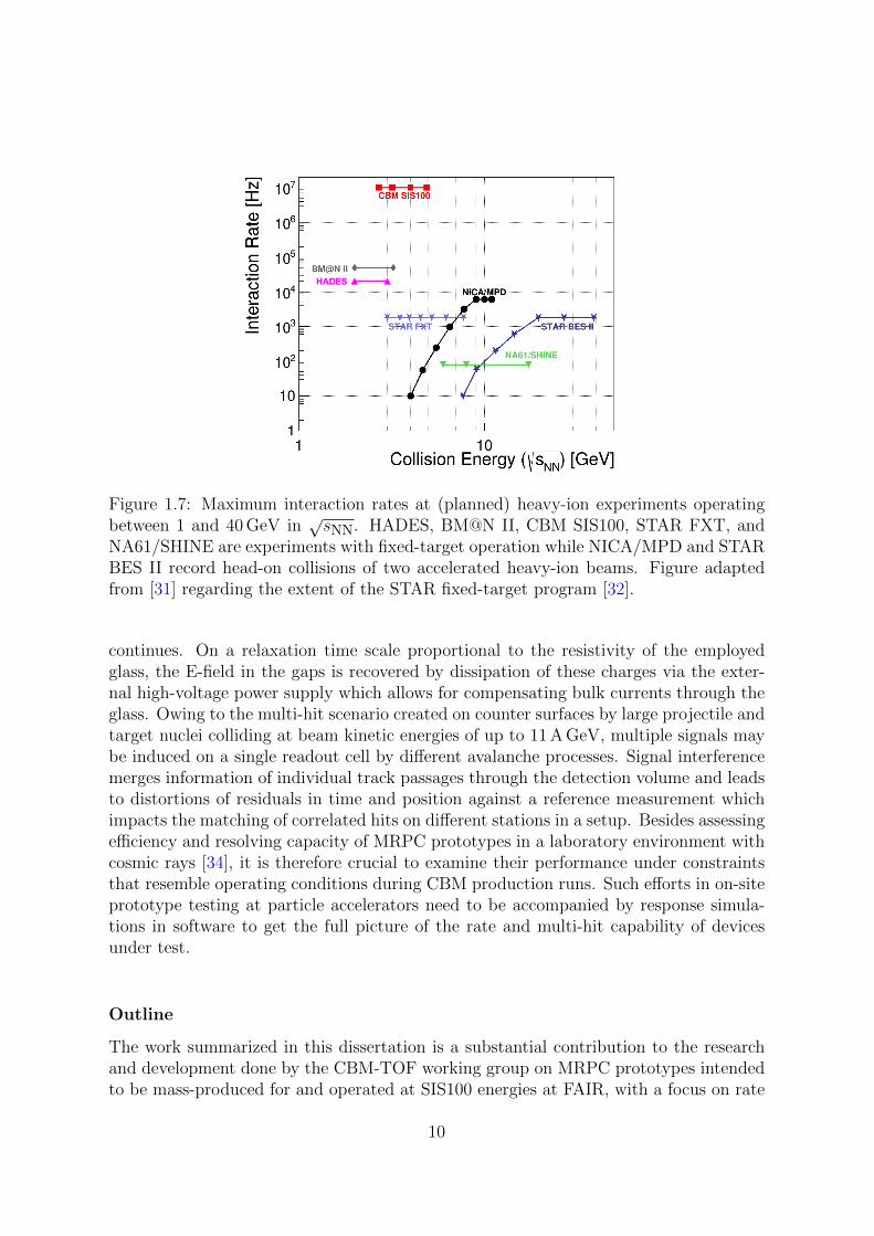
Figure 1.7: Maximum interaction rates at (planned) heavy-ion experiments operatingbetween 1 and 40 GeV in

√sNN. HADES, BM@N II, CBM SIS100, STAR FXT, and

NA61/SHINE are experiments with fixed-target operation while NICA/MPD and STARBES II record head-on collisions of two accelerated heavy-ion beams. Figure adaptedfrom [31] regarding the extent of the STAR fixed-target program [32].

continues. On a relaxation time scale proportional to the resistivity of the employedglass, the E-field in the gaps is recovered by dissipation of these charges via the exter-nal high-voltage power supply which allows for compensating bulk currents through theglass. Owing to the multi-hit scenario created on counter surfaces by large projectile andtarget nuclei colliding at beam kinetic energies of up to 11 A GeV, multiple signals maybe induced on a single readout cell by different avalanche processes. Signal interferencemerges information of individual track passages through the detection volume and leadsto distortions of residuals in time and position against a reference measurement whichimpacts the matching of correlated hits on different stations in a setup. Besides assessingefficiency and resolving capacity of MRPC prototypes in a laboratory environment withcosmic rays [34], it is therefore crucial to examine their performance under constraintsthat resemble operating conditions during CBM production runs. Such efforts in on-siteprototype testing at particle accelerators need to be accompanied by response simula-tions in software to get the full picture of the rate and multi-hit capability of devicesunder test.

Outline

The work summarized in this dissertation is a substantial contribution to the researchand development done by the CBM-TOF working group on MRPC prototypes intendedto be mass-produced for and operated at SIS100 energies at FAIR, with a focus on rate

10

and hit-multiplicity aspects concerning the evaluation of detector performance whichare systematically investigated in experimental and simulated collision data for the firsttime in a synoptic fashion. In Chap. 2, the CBM experiment at FAIR is introduced, em-phasizing in particular its TOF subsystem and the MRPC detector technology involved.Chapter 3 concentrates on describing a particular test beam conducted at CERN/SPSin February/March 2015 which is embedded in a series of prototype tests to which thiswork contributed primarily with the set-up and operation of a data acquisition systemin both hardware and software. For instance, corresponding algorithms were designedfor the calibration and synchronization of raw data. In the selected test beam, a proto-type equipped with special low-resistive glass, aiming at a high rate capability by shortrecovery times for the electric field in the gaps, and a counter composed of commonglass plates were exposed to moderate flux conditions in a multi-hit environment. Thisexperimental scenario which is assessed in detail by a dedicated Monte Carlo study fa-cilitates a direct comparison of the respective response behavior, providing two referencecases for simulations. The latter are based on a novel parametrization of the MRPCresponse function, presented in Chap. 4, which features a sensitivity to both incidentparticle flux and track multiplicity on the counter surface, implementing the time-baseddigitization strategy of CBM for the TOF subsystem. An existing event-based solutionlacks this functionality and is replaced by a closer description of the physical reality.Results obtained for real and virtual prototypes are compared in Chap. 5 with regard toperformance and matching quality as a function of both average hit multiplicities in thesetup and irradiation time. At the end of the chapter, an application of the developedresponse model at the ongoing “mini”-CBM (mCBM) experiment [35] is discussed. Asummary of the entire work is given in Chap. 6.

11

12

CHAPTER 2

THE CBM EXPERIMENT AT FAIR

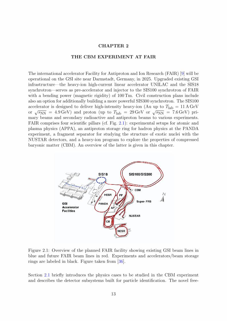
The international accelerator Facility for Antiproton and Ion Research (FAIR) [9] will beoperational on the GSI site near Darmstadt, Germany, in 2025. Upgraded existing GSIinfrastructure—the heavy-ion high-current linear accelerator UNILAC and the SIS18synchrotron—serves as pre-accelerator and injector to the SIS100 synchrotron of FAIRwith a bending power (magnetic rigidity) of 100 Tm. Civil construction plans includealso an option for additionally building a more powerful SIS300 synchrotron. The SIS100accelerator is designed to deliver high-intensity heavy-ion (Au up to Tlab = 11 A GeVor√sNN = 4.9 GeV) and proton (up to Tlab = 29 GeV or

√sNN = 7.6 GeV) pri-

mary beams and secondary radioactive and antiproton beams to various experiments.FAIR comprises four scientific pillars (cf. Fig. 2.1): experimental setups for atomic andplasma physics (APPA), an antiproton storage ring for hadron physics at the PANDAexperiment, a fragment separator for studying the structure of exotic nuclei with theNUSTAR detectors, and a heavy-ion program to explore the properties of compressedbaryonic matter (CBM). An overview of the latter is given in this chapter.

Figure 2.1: Overview of the planned FAIR facility showing existing GSI beam lines inblue and future FAIR beam lines in red. Experiments and accelerators/beam storagerings are labeled in black. Figure taken from [36].

Section 2.1 briefly introduces the physics cases to be studied in the CBM experimentand describes the detector subsystems built for particle identification. The novel free-

13

streaming readout paradigm of CBM is sketched in Sec. 2.2. Section 2.3 addresses thesoftware framework CbmRoot which serves as development platform for the algorithmsoutlined in chapters 3, 4, and 5. In Sec. 2.4, the time-of-flight (TOF) subdetector andthe underlying multi-gap resistive plate chamber (MRPC) technology are discussed.

2.1 Physics observables and detection instruments

The design of the CBM spectrometer is optimized for measuring the most relevantprobes of high-density QCD matter in the SIS100 energy range with unprecedented ac-curacy. Apart from the significance of observables related to strangeness—multi-strange(anti-)baryons, (double-Λ) hypernuclei, deeply-bound strange objects, etc.—for under-standing the evolution of the collision fireball (cf. Chap. 1), the importance of measuringdileptons (pairs of a lepton and an antilepton), particles carrying open or hidden charm,event-by-event fluctuations of conserved quantities, and the collective flow of hadronsfrom the collision zone has constrained the detector layout [31].Dileptons (e+e− and µ+µ−) are penetrating probes of the baryon-dense collision zonedue to their ignorance of the strongly interacting medium which they are produced in.They originate either from virtual photons that are radiated by the fireball during itsentire evolution or from dileptonic decays of low-mass vector mesons (ρ, ω, φ) in themedium. The latter mechanism allows for studying the in-medium properties of vectormesons—in particular the spectral function of the ρ meson—which might unveil a par-tial restoration of chiral symmetry in the hot and dense zone. Charm can be studied atSIS100 energies both above (in proton-induced reactions) and below (in heavy-ion reac-tions) the kinetic production threshold. Hadrons containing charm quarks are assumedto be formed in the initial stage of the collision. The relative yields of charmonium, i.e.the J/ψ meson (cc), and open-charm states like D+ (cd), D− (dc), D0 (cu), and D0 (uc)are sensitive to partonic degrees of freedom which lead to charmonium suppression inthe medium. Applying a thermal model, higher-order moments of event-by-event fluc-tuations of baryon number, strangeness, and electric charge in certain regions of phasespace are expected to be influenced by a possible critical endpoint in the phase diagramif conditions during the fireball evolution are appropriate. The dependence of the ex-cess kurtosis times the squared standard deviation, κσ2, of the net-proton multiplicitydistribution on collision energy is considered a promising observable with this respect.The pressure gradient created in the early fireball drives a collective flow of final-statehadrons with regard to the reaction plane that is spanned by the beam axis and the im-pact parameter vector which connects the centers of the colliding nuclei. Its anisotropiccomponents, the directed (in-plane) flow of strength v1 and the elliptic (out-of-plane)flow of strength v2, are dependent on the nuclear equation of state (EOS) and thus carryinformation on its properties in the dense medium.All probes sketched above have in common that either no related data exist at all in theSIS100 energy range or available statistics are insufficient for a comprehensive physicspicture. The CBM apparatus (cf. Fig. 2.2) will contribute new discoveries and fill exist-ing gaps by the interplay of its detector subsystems.

14

Figure 2.2: Model of the experimental setup in the future CBM cave comprising theHADES spectrometer and the CBM experiment. The beam enters the cave from theleft-hand side. HADES is located on the dark-colored platform on the left while CBMcomponents start on the grey-colored concrete block in the center. A superconductingdipole magnet houses the target, a micro-vertex detector (MVD), and a silicon track-ing system (STS). Further downstream, a ring-imaging Cherenkov (RICH) detector islocated that can be replaced by muon chambers (MuCh). Behind the RICH detector,a transition radiation detector (TRD), a time-of-flight (TOF) wall, an electromagneticcalorimeter (ECAL), and a projectile spectator detector (PSD) complete the setup. Fig-ure provided by the CBM Collaboration.

Superconducting dipole magnet

The H-type dipole magnet [37, 38] generates in its gap of 1 m along the beam axis avertical magnetic field with a bending power of 1 Tm. This is necessary for precisemomentum determination (∆p/p < 1 %) of charged particles bent in the magnetic fieldwith the Micro-Vertex Detector and the Silicon Tracking System both residing in the gapof the magnet. It comprises two circular superconducting coils in two separate cryostats.The maximum stored energy amounts to 5.15 MJ at an operating current of 686 A.

Micro-vertex detector (MVD)

Measuring open charm at SIS100 energies requires determining the secondary decayvertices of D mesons with extremely high precision. Identifying a vertex of D mesonshadronically decaying into pions and kaons, e.g. D+ → K−π+π+ or D0 → K−π−π+π+,

15

is complicated by background from pions and kaons which are promptly emitted fromthe collision zone, in particular if D meson multiplicities are low as in the SIS100 case. Inaddition, the mean free paths of D+/− (cτ = 311.8µm) and D0 (cτ = 122.9µm) in thelaboratory at γ = 1 are by two orders of magnitude smaller than for Λ (cτ = 7.89 cm), Ξ(cτ = 4.91 cm), and Ω (cτ = 2.46 cm) hyperons. The dedicated Micro-Vertex Detector(MVD) [39] consists of four layers of highly granular CMOS monolithic active pixelsensors (MAPS) which are positioned between 5 and 20 cm downstream in the gap ofthe dipole magnet inside the vacuum vessel of the target. The vacuum condition and thevery low material budget per sensor (50µm thickness) are supposed to reduce multiplescattering of the decay products in the detector. Decay vertices of D mesons can beresolved with an uncertainty of only 50µm along the beam axis. Information fromthe MVD can also improve the tracking capability of the Silicon Tracking System atp < 0.5 GeV/c. Due to the limited readout speed of the MAPS technology which wouldlead to a pile-up of events at high beam–target interaction rates and radiation toleranceconstraints in close vicinity to the target, the MVD is the only subsystem that will beoperated at 300 kHz instead of 10 MHz which is the design value for CBM.

Silicon tracking system (STS)

Momentum determination of primary and secondary heavy-ion collision products is akey to particle identification (PID). An arrangement of several parallel tracking lay-ers capable of performing high-resolution two-coordinate measurements of traversingcharged particles which are bent in a magnetic dipole field further allows for geomet-rical track reconstruction. This, in turn, enables a purely topological reconstruction ofshort-lived reaction products such as hyperons by relying only on track information oftheir hadronic daughter particles without a priori identifying their species. The physicsprogram of CBM which aims at measuring rare probes by their decay products at sus-tained interaction rates of 10 MHz is instrumentally based on its Silicon Tracking System(STS) [40, 41]. The eight tracking stations of the STS reside in the gap of the magnetright behind the MVD but outside the target vacuum. They comprise in total about1200 highly segmented double-sided silicon micro-strip sensors of 300µm thickness. TheSTS covers polar angles θ with respect to the beam axis between 2.5 and 25 for theentire azimuthal angle (φ) range, thus constraining the (large) share of reaction phasespace accessible to CBM. It is designed for efficient track reconstruction (ε > 95 %) andprecise momentum determination (∆p/p < 1 %) of charged particles at momenta above1 GeV/c. Charged track multiplicities of about 350 are faced by the STS in centralAu+Au collisions at Tlab = 8 A GeV. For rare probes with very low yields per eventlike Ω baryons, the combinatorial background of the topological invariant-mass recon-struction can be reduced by PID information provided by an additional time-of-flightmeasurement.

16

Ring-imaging Cherenkov (RICH) detector

The identification of dielectronic decay products (electron–positron pairs) of low-massvector mesons like ρ and ω to beyond charmonium (J/ψ) is one pillar of the dilep-ton program of CBM. Electrons can be identified by means of Cherenkov radiation ine.g. a CO2 radiator gas up to a few GeV/c in momentum where the Cherenkov lightproduced by pions starts to become increasingly indistinguishable from the electronicproduction (momentum threshold: 4.65 GeV/c). In CBM, the Ring-Imaging Cherenkov(RICH) [42, 43] detector achieves pion suppression factors of above 100 for momentaup to 8 GeV/c and is the main dielectron identification tool by matching extrapolatedcharged particle tracks from the STS to Cherenkov rings originating from reflected andfocused Cherenkov radiation. The detector is located behind the dipole magnet andconsists of a 1.7 m long CO2 gas vessel, two segmented spherical-glass focusing mir-rors divided into two halves above and below the beam pipe, and two photodetectorplanes registering the emitted UV light with multi-anode photomultiplier tubes. TheCherenkov rings appearing in the photodetector planes are expected to be formed byabout 20 detected photons.

Muon chambers (MuCh)

The second pillar of the dilepton program of CBM are the measurement of charmoniumvia its decay into µ+µ− pairs and complementary measurements of the dimuonic decaychannels of low-mass vector mesons. The latter contributes to a better understandingof the physical and combinatorial background of lepton pairs due to its fundamentallydifferent sources in the dielectronic and dimuonic channels. Owing to their high pen-etrating power in matter, muon detection systems commonly feature hadron absorberplates behind which only (high-momentum) muons are supposed to not have been sig-nificantly absorbed. The amount of absorber material can be adjusted to the intendedmeasurement campaign. Muons originating from a J/ψ decay would not be considerablysuppressed behind an integrated 250 cm of iron while low-momentum muons from an ωmeson decay would get absorbed by a factor of 10. For low-mass vector meson mea-surements at low beam energies, decay muons can be identified with much less absorbermaterial. The definition of a muon is thus momentum dependent. The Muon Chamber(MuCh) [44, 45] detector of CBM is a compact structure of four alternating absorberand tracking stations. It can replace the RICH detector right behind the magnet formuon measurements. Each tracking station consists of three layers of detector cham-bers, the first two stations being composed of gas electron multipliers (GEM) and thelatter two being made of straw tube detectors. Adding and removing absorber materialdepending on the observable under study is mechanically possible despite of the compactconstruction necessary to reduce the muon background from the weak decays of pionsand kaons. As an additional tracking station the transition radiation detector can beused.

17

Transition radiation detector (TRD)

Hypernuclei decay i.a. into doubly charged nuclear fragments (4He and d) which cannotbe separated by the Time-of-Flight system alone if PID information is needed in additionto the decay topology reconstructed based on STS data. Measuring the specific energyloss of these particles would improve the reconstruction capability of CBM with respectto hypernuclei. Electron identification by the RICH detector is limited in momentum dueto the onset of pionic Cherenkov radiation. Both issues are addressed by the TransitionRadiation Detector (TRD) [46, 47] positioned behind the RICH detector and in frontof the Time-of-Flight wall. The TRD station consists of four detector layers which arecomposed of individual detector modules each comprising a radiator and a Xe/CO2 basedmulti-wire proportional chamber (MWPC). Only electrons above 1 GeV/c in momentumproduce soft X-ray photons in the radiator which are detected in the MWPC in additionto the particle’s energy loss due to ionization in the gas. The signature that electronsleave in the TRD is thus unique. Providing an electron transition radiation efficiency of90 % and a pion suppression factor of 10–20, the TRD improves the quality of dielectronmeasurements in CBM. It also serves as an intermediate tracking station which positivelycontributes to matching STS tracks with hits in the Time-of-Flight wall.

Time-of-flight (TOF) wall

Pions, kaons, and protons (particles and antiparticles) which are either direct probes ofthe collision zone or “long-lived” daughter particles of rare probes such as hyperons canbe unambiguously identified by their mass and their charge. If the momentum is known,the particle mass can be calculated from its velocity which, in turn, requires knowledge ofthe time difference between a particle’s production and its detection and of the associatedtrajectory length. To separate π, K, and p up to a few GeV/c in momentum, theresolution of the time-of-flight measurement is the limiting factor. The Time-of-Flight(TOF) [48, 49] wall of the CBM experiment in combination with an appropriate startdetector solution serves this purpose. A system time resolution of better than 80 psand a detection efficiency of above 95 % make it the backbone of hadron identificationin CBM. It not only enables PID of primary pions, kaons, and protons emitted fromthe collision zone but also substantially reduces combinatorial background in invariant-mass spectra of hyperons generated from STS track information. The worse the signalover background ratio of rare probes, the more important an independent time-of-flightmeasurement becomes, as for Ω+ → ΛK+ and Ω− → ΛK−. The wall covers an activearea of about 120 m2 and is positioned at 6 m downstream the beam line. Large-areamulti-gap resistive plate chambers (MRPCs) varying in size with a high rate capabilityare used as detection technology. The TOF system is described in more detail in Sec. 2.4.

18

Electromagnetic calorimeter (ECAL)

Direct photons which are produced in the early stage of the collision carrying undisturbedinformation of the conditions at production time through the fireball can be detected byelectromagnetic showers in lead absorber plates. This argument extends to the measure-ment of the (semi-)photonic decay channels of π0 → γγ, η → γγ, and ω → π0γ which isnecessary for counter-checking the contribution of the corresponding Dalitz decays—e.g.π0 → γe+e−—to dielectron measurements. In CBM, the Electromagnetic Calorimeter(ECAL) [50] measures photons by the energy deposited in a “shashlik”-type stack oflead absorber plates interspaced with scintillator tiles as active material. Wavelength-shifting fibers penetrate the stack orthogonally to transport the visible light producedin the scintillation material from the radiated shower energy to photomultipliers. The1088 “shashlik” stacks of dimensions 6 × 6 cm2 are grouped in two rectangular blocksabove and below the beam pipe which can be rearranged to accommodate differentexperimental conditions.

Projectile spectator detector (PSD)

The analysis of event-by-event fluctuations crucially depends on precise knowledge ofthe centrality class of the event, i.e. how central the projectile nucleus hit the targetnucleus. Collective flow of hadrons can only be studied quantitatively if the reactionplane can be well defined. Both event characteristics are linked to the number of pro-jectile nucleons that do not participate in the collision (spectators) and can be deducedfrom the energy distribution of projectile fragments and forward going particles movingclose to the beam axis. The Projectile Spectator Detector (PSD) [51, 52] designed asa compensating hadronic calorimeter performs the determination of collision centralityclasses with an uncertainty of better than 10 % and resolves the reaction plane anglewith a worst-case accuracy of 40 . In total, the PSD comprises 44 modules each madeof 60 lead/scintillator sandwiches of transverse dimensions 20 × 20 cm2. Scintillationlight is collected by fiber tiles which are read out by micro-pixel avalanche photodiodes(MAPD).

2.2 Data acquisition and online event selection

Identifying candidate events that might contain rare probes like open charm or multi-strange baryons at continuous beam–target interaction rates of 10 MHz does not onlyimpose challenging requirements on the individual subsystems of CBM, e.g. a high ratecapability and—in the same time—a high radiation tolerance, but also necessitates anovel readout paradigm concerning each subsystem and the entire apparatus. Triggerpatterns for rare-probe detection cannot be implemented straightforwardly in hardwareas a significant share of detector raw data needs to be processed, including track recon-struction, to find signatures of D meson or Ω baryon decay topologies in the data. Thesubsystems in CBM thus push all digitized detector response messages autonomously

19

towards a high-performance computing farm which serves as a first-level event selector(FLES) [53]. In fact, no low-level event filtering is done prior to this stage.

CBM cave CBM building Green IT Cube

~700 m~80 m

Figure 2.3: Sketch of the self-triggered readout concept of the CBM experiment. Nu-merous front-end boards (FEB) hosting the front-end digitization electronics push anyavailable raw data to a layer of (common) readout boards (CROB) which, in turn, con-centrate many electrical input connections into single optical data uplinks towards thecommon readout interface (CRI) layer. The CRI boards serve as gateway to the FLESnetwork. The latter consists of input and compute nodes. A Timing and Fast Control(TFC) system keeps the entire readout chain in synchronization while the ExperimentControl System (ECS) implements configuration access and readout of control registers.Details are explained in the text. For simplification, the sketch focusses on the data flowof only a few FEBs via CROBs to a single CRI board residing—together with others—inone of many FLES input nodes. Figure adapted from [54].

The data flow from the detector subsystems to the FLES is sketched in Fig. 2.3. All ana-log detector signals exceeding some detection threshold are digitized by the subsystem-specific front-end electronics (FEE) integrated into front-end boards (FEB) which aremounted in close vicinity to the detection instruments. In a self-triggered manner, i.e.without any readout request, these data are pushed upon availability to an aggregationlayer of readout boards (CROB) via electrical connections. The CROB layer [55] is dataagnostic and concentrates several electrical FEB inputs into a single optical output fordata transport (∼ 80 m) from the CBM cave underground to the ground level of theCBM building. In the absence of a global readout trigger signal that would associateraw data with an event, the detector information needs to be synchronized across all

20

subsystems to preserve the physical correlation of data in time for the FLES algorithmsto reconstruct events both in time and space. The time stamps that are generated by thefront-end electronics along with detector response messages thus need to be derived froma common reference clock signal which is provided by the Timing and Fast Control (TFC)system [56]. The value of a time stamp corresponds to the number of reference clockcycles the digitization electronics have counted at the point in time when digitizationtakes place. A system-wide synchronous reset of these clock-cycle counters is triggeredby critical low-latency synchronization messages generated by the TFC system. Boththe reference clock signal and synchronization messages are transported to the front-endlayer via downlinks of the CRI boards which receive the aggregated data streams fromthe front-end electronics. The Common Readout Interface is the first stage in the read-out chain which explicitly reads the time stamps of incoming data to partition them intodata containers representing a fixed time interval of about 1µs. These “microslices” ofdata contain an index which is incremented synchronously throughout all CRI boards inCBM which allows for matching data between different (parts of) subsystems. Depend-ing on the experimental snapshot which is represented by a microslice, its size is—incontrast to its duration—variable. The CRI boards are intended to be plugged into theFLES input nodes located in the CBM building. They forward the system clock signaland synchronization commands from the TFC system to the front-end layer and sendand receive slow-control commands (setting of FEE configuration registers, reading ofFEE status registers) issued by the Experiment Control System (ECS).Via an optical fiber connection of 700 m, the FLES input nodes form a high-throughputInfiniBand network with the FLES compute nodes that are located in the Green ITCube of FAIR, a six-story high-performance computing center. The purpose of thisnetwork and of the inter-node data management software FLESnet operating on it isthe encapsulation of a series of microslice containers originating from different detec-tor subsystems into a self-contained “timeslice” (cf. Fig. 2.4, left) of data that can beindependently processed by event-reconstruction algorithms on a single FLES computenode. Each compute node processes data from a different timeslice, with some overlap intime to account for physical events possibly split by a timeslice border. At beam–targetinteraction rates of 10 MHz in the SIS100 energy range, the raw data rate in the FLES isestimated to be on the order of 100 GB/s [49]. Even if such a high sustained rate couldbe permanently stored for offline analysis, it would not be very efficient given the lowmultiplicities of rare probes that CBM addresses. Huge amounts of data would need tobe filtered in search of rare-probe signatures and mostly be discarded in the end. CBMis designed to perform this operation online prior to permanent storage. Depending onthe physics observable under study, a certain share of raw data, mostly from the STSfor track reconstruction, possibly extended to data from a PID detector like TOF, i.e. asubset of timeslice components is inspected online on the FLES compute nodes to esti-mate by partial event reconstruction if the data under study are a promising candidatefor a detailed offline analysis. By applying this online data reduction scheme, CBM aimsat a final data archival rate of 1 GB/s only.The tracking algorithms devoted to online event selection need to be efficient, fast,and optimized for vectorized and parallel computations, utilizing modern many-core

21

Timeslice

DESC

MC

0

DESC

MC

1

CONT

ENT

MC

0

CONT

ENT

MC

1. . .

Com

pone

nt 0

DESC

MC

99

CONT

ENT

MC

99

DESC

MC

100

CONT

ENT

MC

100

DESC

MC

0

DESC

MC

1

CONT

ENT

MC

0

CONT

ENT

MC

1

. . .

Com

pone

nt 1

DESC

MC

99

CONT

ENT

MC

99

DESC

MC

100

CONT

ENT

MC

100

. . .

DESC

MC

101

CONT

ENT

MC

101

DESC

MC

102

CONT

ENT

MC

102

Core region Overlap regionTime Time [ns]4300 4350 4400 4450 4500 4550 4600

Ent

ries

1

10

210

Figure 2.4: A fixed amount of consecutive microslices (here: MC for micro-container)from different components (usually a part of a detector subsystem) of the experimentform a timeslice container consisting of a core and an overlap region in case of eventsplitting across borders (left plot, taken from [57]). Simulated four-dimensional trackreconstruction (black bars) from detector hit information (cyan bars) within a timesliceat 10 MHz interaction rate distributing time intervals between events exponentially (rightplot, taken from [58]).

CPU/GPU computing architecture. The FLES software package [58] which meets thesedemands requires as input a geometric description of the tracking detector and hits ofcharged particles intersecting the geometry. A prerequisite is that the latter are built,also online, from detector raw data which depends on an efficient online calibration ofthe digital detector response. First, a track-finding stage based on a Cellular Automaton(CA) groups detector hits into tracks in time and space [59] which are then fitted by aKalman Filter (KF) to precisely estimate the track parameters. A good track-fit qualityhelps reducing the combinatorial background of invariant-mass spectra of topologicallyreconstructed short-lived particles.After fitting, tracks are combined into clusters which fill a series of non-empty histogrambins in time (cf. Fig. 2.4, right) and can thus be identified as tracks belonging to the samephysical event. This histogram method does not allow for disentangling event overlapswhich occur in 22 % of cases at collision rates of r = 10 MHz, assuming an exponentiallydistributed time between two consecutive collisions,

f(t) dt = e−rtr dt, (2.1)

and a time distribution of hits from a single event in the detector of 25 ns. Instead, thedifferent primary vertices of overlapping events (four-dimensional interaction points)would need to be determined by extrapolating fitted tracks to the target zone, followedby a multi-vertex analysis. Identifying event structures in the time distribution of rawdata directly [60] is also possible but much more susceptible to background from deltaelectrons produced in the target and detector noise due to the lack of correlation intro-duced by tracking.After event building from particles that leave tracks in the detector, the KF Particle

22

Finder package reconstructs short-lived particles, i.e. the rare probes of interest whichdecay ahead of the tracking stations, from the tracks of their long-lived daughter par-ticles. Ultimately, events of interest are selected based on the trigger signatures foundduring online reconstruction and written to disk. If the information about the eventtopology reconstructed from STS tracks alone is not sufficient to take a trigger decision,track following and propagation methods to PID instruments further downstream usingSTS tracks as seeds [61] need to be run online at additional computational cost.

2.3 Simulation and reconstruction in CbmRoot

A feasibility study of the online event-selection strategy developed by CBM is a synergyof hardware and software aspects. On the hardware side, prototypical high-throughputreadout-chain components need to be tested under realistic in-beam conditions. Con-cerning software, it is necessary to realistically simulate a free-streaming data flow fromthe front-end digitizers to the computing farm in order to design online reconstructionalgorithms to be run on the FLES. As most heavy-ion experiments of the past could relyon hardware-triggered events as input to their reconstruction and analysis frameworks,CBM is required to implement—building upon familiar event-by-event processing—adata-handling concept as well as algorithms that operate on containers representingfixed time intervals, i.e. timeslices.The standard framework for future FAIR experiments comprising simulation, reconstruc-tion, and data-analysis functionality, FairRoot [62], makes use of existing event-basedinfrastructure provided by ROOT [63]. CbmRoot, in turn, inherits from FairRoot andimplements experiment-specific data classes. The entire code is compiled into sharedlibraries which are loaded on demand by the ROOT executable which processes user-supplied configuration macros for specific purposes. At the heart of a FairRoot run, therun manager class governs initialization and execution of a hierarchy of tasks (implemen-tations of ROOT’s TTask class) each of which processes the output data of the precedingtask and generates input data for its successor. All tasks are sequentially executed bythe run manager to transform a set of initial data classes (e.g. detector raw data) to thedesired output format (e.g. tracks). If several such sets of data (events) are available,the run manager repeatedly calls the sequence of registered tasks, once for each event.All data of the same type produced by a task within the scope of one event reside ina TClonesArray entry of a TTree branch, utilizing functionality of ROOT. Branchesdeclared persistent are serialized and streamed into a ROOT output file which mightserve as input to a subsequent FairRoot run.As the TClonesArray container is indifferent to being considered an event or a timeslice,the consequential starting point for time-based data handling is re-interpreting it as thelatter [64]. However, nuclear collision seeds produced by microscopic transport codeslike UrQMD [65, 66] or PHSD [18, 19] for a simulation are propagated through a vir-tual description of the detector geometry (cf. Fig. 2.5) by Monte Carlo (MC) transportengines [67] event by event. Primary particles from the collision zone are pushed ontoan event stack and then—in reverse order—transported with a defined step size through

23

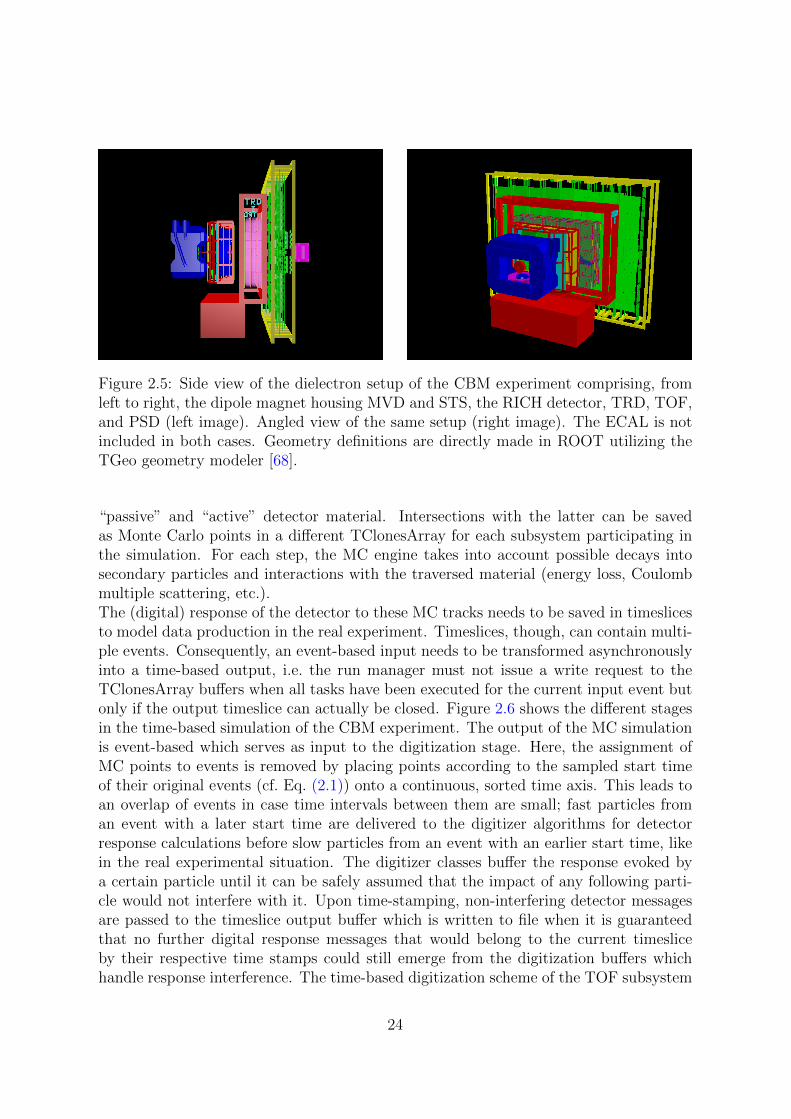
Figure 2.5: Side view of the dielectron setup of the CBM experiment comprising, fromleft to right, the dipole magnet housing MVD and STS, the RICH detector, TRD, TOF,and PSD (left image). Angled view of the same setup (right image). The ECAL is notincluded in both cases. Geometry definitions are directly made in ROOT utilizing theTGeo geometry modeler [68].

“passive” and “active” detector material. Intersections with the latter can be savedas Monte Carlo points in a different TClonesArray for each subsystem participating inthe simulation. For each step, the MC engine takes into account possible decays intosecondary particles and interactions with the traversed material (energy loss, Coulombmultiple scattering, etc.).The (digital) response of the detector to these MC tracks needs to be saved in timeslicesto model data production in the real experiment. Timeslices, though, can contain multi-ple events. Consequently, an event-based input needs to be transformed asynchronouslyinto a time-based output, i.e. the run manager must not issue a write request to theTClonesArray buffers when all tasks have been executed for the current input event butonly if the output timeslice can actually be closed. Figure 2.6 shows the different stagesin the time-based simulation of the CBM experiment. The output of the MC simulationis event-based which serves as input to the digitization stage. Here, the assignment ofMC points to events is removed by placing points according to the sampled start timeof their original events (cf. Eq. (2.1)) onto a continuous, sorted time axis. This leads toan overlap of events in case time intervals between them are small; fast particles froman event with a later start time are delivered to the digitizer algorithms for detectorresponse calculations before slow particles from an event with an earlier start time, likein the real experimental situation. The digitizer classes buffer the response evoked bya certain particle until it can be safely assumed that the impact of any following parti-cle would not interfere with it. Upon time-stamping, non-interfering detector messagesare passed to the timeslice output buffer which is written to file when it is guaranteedthat no further digital response messages that would belong to the current timesliceby their respective time stamps could still emerge from the digitization buffers whichhandle response interference. The time-based digitization scheme of the TOF subsystem

24

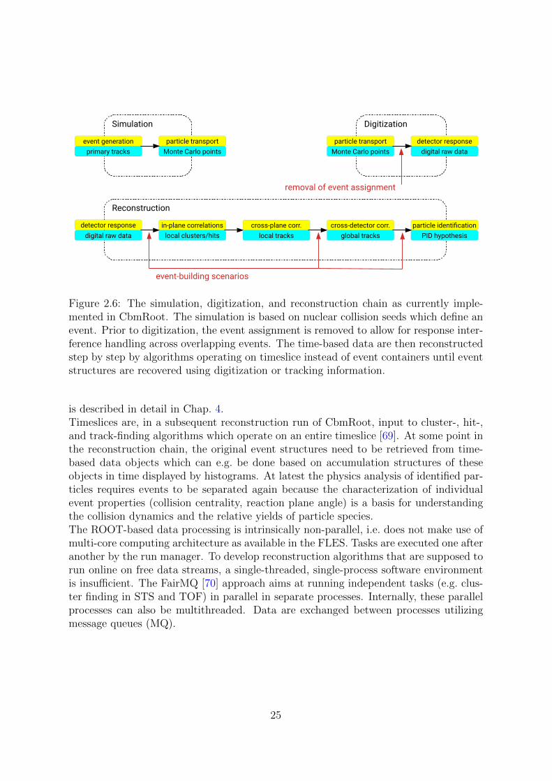
Reconstruction

in-plane correlationslocal clusters/hits

detector responsedigital raw data

cross-plane corr.local tracks

cross-detector corr.global tracks

particle identificationPID hypothesis

Simulation

particle transportMonte Carlo points

event generationprimary tracks

event-building scenarios

removal of event assignment

Digitization

detector responsedigital raw data

particle transportMonte Carlo points

Figure 2.6: The simulation, digitization, and reconstruction chain as currently imple-mented in CbmRoot. The simulation is based on nuclear collision seeds which define anevent. Prior to digitization, the event assignment is removed to allow for response inter-ference handling across overlapping events. The time-based data are then reconstructedstep by step by algorithms operating on timeslice instead of event containers until eventstructures are recovered using digitization or tracking information.

is described in detail in Chap. 4.Timeslices are, in a subsequent reconstruction run of CbmRoot, input to cluster-, hit-,and track-finding algorithms which operate on an entire timeslice [69]. At some point inthe reconstruction chain, the original event structures need to be retrieved from time-based data objects which can e.g. be done based on accumulation structures of theseobjects in time displayed by histograms. At latest the physics analysis of identified par-ticles requires events to be separated again because the characterization of individualevent properties (collision centrality, reaction plane angle) is a basis for understandingthe collision dynamics and the relative yields of particle species.The ROOT-based data processing is intrinsically non-parallel, i.e. does not make use ofmulti-core computing architecture as available in the FLES. Tasks are executed one afteranother by the run manager. To develop reconstruction algorithms that are supposed torun online on free data streams, a single-threaded, single-process software environmentis insufficient. The FairMQ [70] approach aims at running independent tasks (e.g. clus-ter finding in STS and TOF) in parallel in separate processes. Internally, these parallelprocesses can also be multithreaded. Data are exchanged between processes utilizingmessage queues (MQ).

25

2.4 Time-of-flight measurements with resistive plate chambers

2.4.1 The time-of-flight method

From the curvature of a trajectory in the magnetic dipole field measured by the STSthe momentum and the charge sign of a particle can be deduced but its species cannotbe identified without an additional, independent measurement. For the rare-probe pro-gram of CBM, the identification of abundant charged hadrons (π+, K+, p, and theirantiparticles) in a large share of reaction phase space is essential. Figure 2.7 shows thephase space spanned by lab rapidity and by the ratio of transverse momentum over massaccessible to prompt pions, kaons, and protons at upper-end SIS100 energies.

1− 0 1 2 3 4

[]lab

y

0

0.5

1

1.5

2

2.5

/(m

c) []

t p

210

310

1− 0 1 2 3 4

[]lab

y

0

0.5

1

1.5

2

2.5

/(m

c) []

t p

1

10

210

310

1− 0 1 2 3 4

[]lab

y

0

0.5

1

1.5

2

2.5

/(m

c) []

t p

1

10

210

310

410

510

610

Figure 2.7: Phase space populated by (positively charged) primary pions (left plot),kaons (middle plot), and protons (right plot) originating from 100,000 UrQMD collisionsof gold nuclei at pbeam = 10 A GeV/c with minimum centrality bias. The black linesindicate constant total laboratory momentum (from left to right: 0.5, 1.0, 2.0, 4.0, 8.0,and 16.0 GeV/c) while the blue lines represent the geometrical acceptance of the STS,between 2.5 (right line) and 25 (left line) in polar angle.

In particular, the particle identification concept needs to be capable of cleanly sepa-rating pions from kaons which is challenging due to their similar masses (0.140 GeV/c2

and 0.494 GeV/c2, respectively) on the hadronic mass scale. To disentangle kaons frompions at mid-rapidity (here: y0 = 1.53), the separation power of the PID method forthis case should cover the momentum range up to 3–4 GeV/c. This can be achievedby the time-of-flight method [71] which makes use of the relativistic relation betweenthe (squared) particle mass m, its momentum p, its trajectory length L, and its time offlight t,

m2 =p2

c2

(c2t2

L2− 1

). (2.2)

The relative uncertainty of the squared mass measurement, assuming Gaussian errors ofindividual contributions,

σm2

m2= 2

√(σpp

)2

+(1 + (βγ)2

)2((σtt

)2+(σLL

)2), (2.3)

26

is by a factor of about 13 (βγ ∼ 3.5 for minimum ionizing particles) more susceptible toerrors in determining the time of flight and the track length than to errors in momentum.Usually, the bottleneck is the resolution of the time of flight which consists of a starttime and a stop time measurement.Solving Eq. (2.2) for t and considering the limit pmc leads to the expression

|t1 − t2| =Lc

2p2|m2

1 −m22| (2.4)

for the absolute difference in time of flight between two different particle species at agiven momentum and trajectory length. The separation power with respect to the TOFmeasurement is then given by

nσt =|t1 − t2|σt

=Lc

2p2σt|m2

1 −m22|. (2.5)

Assuming the TOF error to be the dominating contribution to the squared-mass uncer-tainty (cf. Eq. (2.3)) and expressing σt in Eq. (2.5) by σ

m2 only depending on σt,

σm2 =

2p2

Lcβσt, (2.6)

one obtains a relation between the absolute difference of two squared particle masses,the required TOF separation power, and the squared-mass resolution,

|m21 −m

22| = β nσt σm2 . (2.7)

In the relativistic limit (β → 1), the widths of squared particle-mass distributions shouldbe similar across particle species and only depend on momentum and trajectory length(cf. Eq. (2.6)). A TOF separation power of nσt = 3 would, for instance, be achieved ifthe 1.5-sigma lines of two neighboring squared-mass distributions just crossed each other.Figure 2.8 shows an idealized PID scenario utilizing the separation-power formalism ofEq. (2.7) based on simulated Monte Carlo data. The intersection points of the red PIDgate lines indicate the limiting momenta above which the required separation powerdoes not hold anymore, i.e. the squared-mass branch of one particle species becomesincreasingly contaminated by its neighbor(s). The limiting momenta depend stronglyon the system time resolution σt, decreasing for π/K separation from about 4.3 GeV/cat σt = 50 ps to 3.5 GeV/c at σt = 80 ps to 3.1 GeV/c at σt = 100 ps.According to Eq. (2.6), larger distances between production vertex and detection pointlead to narrower m2-distributions and thus improve the PID capability. On the otherhand, the limited mean free path of K mesons in the laboratory (γcτ = 8.4 m at p =1 GeV/c) places additional constraints on the positioning of a TOF system with respectto the target. In the end, the position needs to be optimal for the physics observableunder study. The bend towards higher m2-values observable in the proton branch atlow momenta is due to energy loss in the material between target and TOF wall andneeds to be corrected for in the final experiment. At higher momenta, the distribution

27

0 2 4 6 8 10

[GeV/c]lab

p

1−

0

1

2

3]4/c2

[GeV

2 m

1

10

210

310

410

0 2 4 6 8 10

[GeV/c]lab

p

1−

0

1

2

3]4/c2

[GeV

2 m

1

10

210

310

410

0 2 4 6 8 10

[GeV/c]lab

p

1−

0

1

2

3]4/c2

[GeV

2 m

1

10

210

310

410

Figure 2.8: Squared particle masses of primary pions, kaons, and protons as a func-tion of laboratory momentum obtained from the MC sample described in Fig. 2.7. Themomentum is the initial value from the production vertex. Exact time-of-flight andtrajectory-length information is provided by the MC track propagator. When a trajec-tory intersects an active geometric volume of the TOF wall (positioned at 6 m < L < 7 mfrom the target, cf. Fig. 2.5), the time is stopped. For realistic trajectories, four pas-sages through STS tracking planes are requested per track. TOF values are smearedwith Gaussian resolutions of 50 ps (left plot), 80 ps (middle plot), and 100 ps (right plot).The red lines correspond to second-order polynomial fits to the 1.5-σ values extractedfrom the sum of three equal-σ Gaussian fit functions which are centered about the truesquared masses of the particles in every squared-mass slice along the momentum axis.

0 0.5 1

]4/c2 [GeV2m

0

2

4

310×+π+K

p

0 0.5 1

]4/c2 [GeV2m

0

2

4

310×+π+K

p

0 0.5 1

]4/c2 [GeV2m

0

2

4

310×+π+K

p

Figure 2.9: Squared-mass slices of primary pions, kaons, and protons at p = 3 GeV/cextracted from the plots in Fig. 2.8. The colored curves represent the individual Gaussiancontributions of each particle species to the summed Gaussian function which has beenfitted to each squared-mass slice.

of protons can be described by a Gaussian function as in the case of pions and kaons.Figure 2.9 demonstrates the feasibility of the described PID method, at least in the limitof an ideal detector. In the running experiment, the white area in Fig. 2.8 will be coveredwith background resulting—among others—from track-to-hit mismatches between theSTS and TOF subsystems. On the Monte Carlo level, the affiliation of a TOF pointwith a given primary track is known. In Fig. 2.9, one can see how the kaon peak mergeswith the pion peak as the simulated system time resolution worsens. At σt = 100 ps,

28

it could already be difficult to separate kaons from pions up to 3 GeV/c in momentumwith nσt = 3 if the detector response were realistic.For completeness, it shall be pointed out that separating particle species via PID gateson an m2(p)-plot is one particular implementation of the time-of-flight method. In theALICE experiment, for instance, different approaches are combined [72].

2.4.2 Multi-gap resistive plate chambers

A detector technology suitable for charged-hadron identification via time of flight inCBM needs not only to allow for precise time measurements (on the order of 80 ps forthe entire timing system) as shown in the previous subsection. In addition, it must bescalable to a large detection area to cover the geometrical acceptance of the STS takinginto account the trajectory bending in the magnetic field at distances between 6 and10 m from the target as required for hadron separation up to a few GeV/c in momentum.Lastly, the response function of the detector should sustain a high detection efficiencyeven at nominal beam–target interaction rates of 10 MHz which exposes the TOF wallto particle fluxes from a few tens of kHz/cm2 in the inner zone (even above 100 kHz/cm2

in the immediate vicinity of the beam pipe) to below 1 kHz/cm2 at the periphery (cf.Fig. 2.10). Currently, only (large-area) multi-gap resistive place chambers (MRPCs)meet the challenging technological demands of the TOF system at an affordable cost

600− 400− 200− 0 200 400 600

x [cm]

400−

200−

0

200

400

y [c

m]

1

10

210

310

410

510

]2 [H

z/cm

Φ p

artic

le fl

ux

Figure 2.10: Particle flux through the CBM TOF wall positioned between 6 and 7 mfrom the target at a beam–target interaction rate of 10 MHz in cave coordinates xy,integrated in z over the entire support frame. Due to the staggered and partially tiltedplacement of active detector volumes within the frame, the particle flux extrapolatedfrom 100,000 Au+Au events at pbeam = 10 GeV/c with minimum centrality bias onlyapproximately corresponds to the actual flux. Structures visible on the flux plot resultfrom detector volumes overlapping in xy.

29

and provide sufficient design flexibility to adapt to the strongly varying flux conditionsacross the wall. Conceptional details of the TOF wall are given in Sec. 2.4.3.Multi-gap resistive plate chambers [73] utilize the ionization of gas molecules by travers-ing charged particles in an electric field as primary detection process. Electrons strippedoff from their atoms are accelerated towards the anode and ionize further molecules.Subsequently, secondary ionization electrons repeat this procedure which leads to arapid multiplication of electrons developing into a Townsend avalanche containing onthe order of 107 electrons. The probability for an avalanche to consist of n+ 1 electronsat a distance of x + dx from the primary ionization point provided that it comprises nelectrons at x is given by nαdx wherein the Townsend coefficient α states the number ofsecondary electron–ion pairs created per unit length in the gaseous medium dependingon the applied electric field [74]. Similarly, the reattachment of electrons to positivelycharged ions during avalanche formation is described by the attachment coefficient η.Combining both differential detachment and attachment processes in a single formulaand integrating over position yields the expression

N = N0e(α−η)x (2.8)

for the average number of avalanche electrons at a distance of x to the primary ion-ization cluster containing N0 electrons. For a gas mixture typically used in MRPCsof 85 % 1,1,1,2-tetrafluoroethane (C2H2F4), 10 % sulfur hexafluoride (SF6), and 5 %isobutane (C4H10) under atmospheric pressure at room temperature in an electric fieldof 100 kV/cm (α − η ∼ 113/mm [74]), an average avalanche would—according to thesimplified approach described by Eq. (2.8)—consist of 108 electrons after growing for adistance of only 160µm.An MRPC is composed of a stack of rectangular resistive plates made of materials rang-ing from ceramics to common glass (cf. Fig. 2.11(a)). To the external surfaces of theouter plates a high voltage is applied which creates a strong uniform electric field in thegaps between the resistive plates. The inner plates are electrically floating and separatedfrom each other by 100 to 300µm using appropriate spacers like fishing line. These smallgap widths allow for a very large gas gain (high electric field) without forming streamerdischarges in the gaps by stopping the avalanche growth early enough. The onset ofthe latter occurs at above 108 avalanche electrons [76], known as the Raether limit,and involves the production of a large amount of charge which deteriorates the detectorperformance (see below). In addition, strong space-charge effects due to the high chargedensity in the narrow gaps limit the number of electrons in the avalanche.Signal induction on the readout electrodes which are adjacent to but isolated from thehigh-voltage layers (cf. Fig. 2.11(a)) by moving avalanche electrons in any gap startsimmediately after primary ionization and is not hampered by the presence of the resis-tive plates which are transparent for fast induced signals. The current signal inducedby electrons is much bigger than the corresponding signals induced by positively andnegatively charged ions in the avalanche due to the high drift velocity of electrons in thegap. For the above gas mixture in an electric field of 100 kV/cm, electron drift veloc-ities of vdrift ∼ 200µm/ns are achieved [74] which results in signal formation times of

30

+

–

–

+

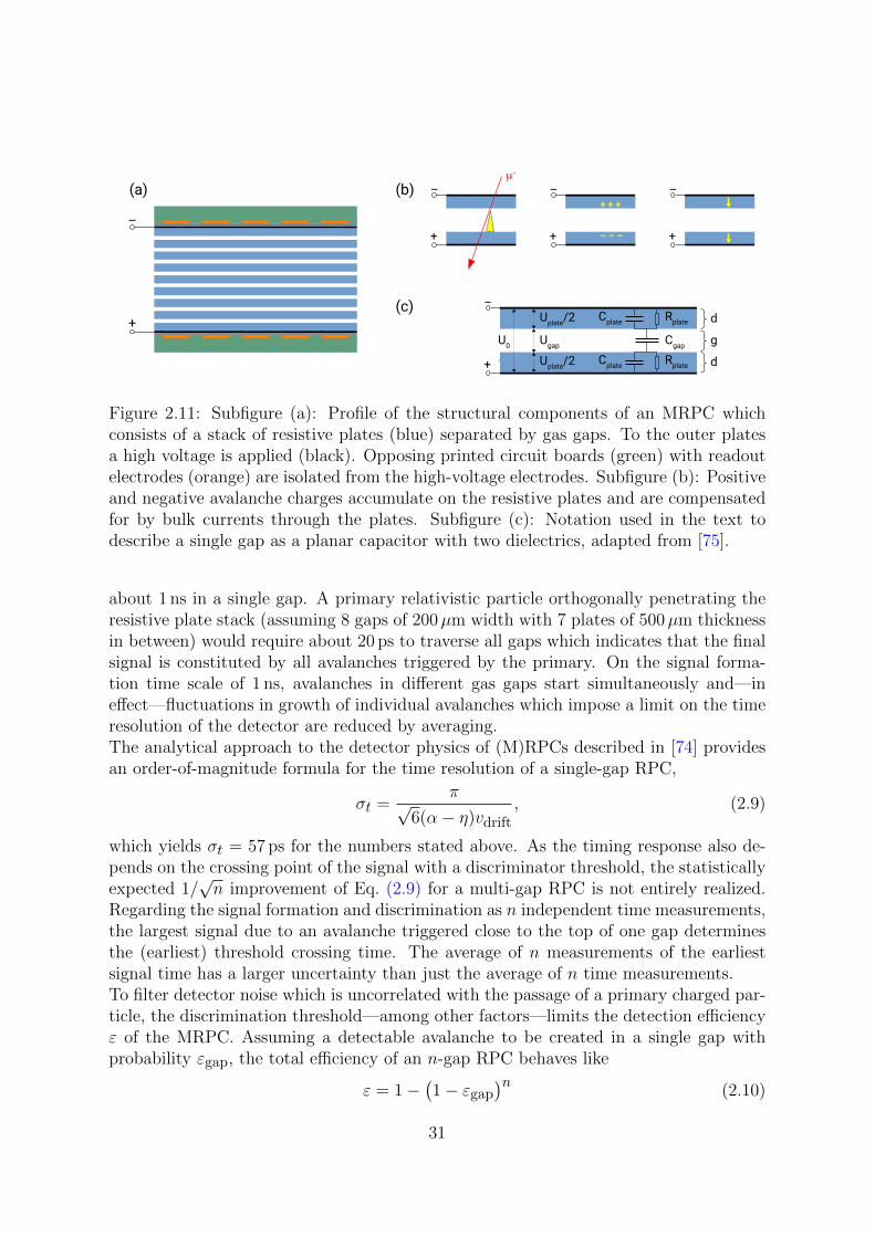
m-

–

+ – – –

+ + + –

+

–

+

U0 Ugap

Uplate/2

Uplate/2

Cgap

Rplate

Rplate

Cplate

Cplate

d

d

g

(a) (b)

(c)

Figure 2.11: Subfigure (a): Profile of the structural components of an MRPC whichconsists of a stack of resistive plates (blue) separated by gas gaps. To the outer platesa high voltage is applied (black). Opposing printed circuit boards (green) with readoutelectrodes (orange) are isolated from the high-voltage electrodes. Subfigure (b): Positiveand negative avalanche charges accumulate on the resistive plates and are compensatedfor by bulk currents through the plates. Subfigure (c): Notation used in the text todescribe a single gap as a planar capacitor with two dielectrics, adapted from [75].

about 1 ns in a single gap. A primary relativistic particle orthogonally penetrating theresistive plate stack (assuming 8 gaps of 200µm width with 7 plates of 500µm thicknessin between) would require about 20 ps to traverse all gaps which indicates that the finalsignal is constituted by all avalanches triggered by the primary. On the signal forma-tion time scale of 1 ns, avalanches in different gas gaps start simultaneously and—ineffect—fluctuations in growth of individual avalanches which impose a limit on the timeresolution of the detector are reduced by averaging.The analytical approach to the detector physics of (M)RPCs described in [74] providesan order-of-magnitude formula for the time resolution of a single-gap RPC,

σt =π√

6(α− η)vdrift, (2.9)

which yields σt = 57 ps for the numbers stated above. As the timing response also de-pends on the crossing point of the signal with a discriminator threshold, the statisticallyexpected 1/

√n improvement of Eq. (2.9) for a multi-gap RPC is not entirely realized.

Regarding the signal formation and discrimination as n independent time measurements,the largest signal due to an avalanche triggered close to the top of one gap determinesthe (earliest) threshold crossing time. The average of n measurements of the earliestsignal time has a larger uncertainty than just the average of n time measurements.To filter detector noise which is uncorrelated with the passage of a primary charged par-ticle, the discrimination threshold—among other factors—limits the detection efficiencyε of the MRPC. Assuming a detectable avalanche to be created in a single gap withprobability εgap, the total efficiency of an n-gap RPC behaves like

ε = 1−(1− εgap

)n(2.10)

31

if each gap is treated as a separate detection instrument which is only approximately thecase because all avalanches created in the stack contribute to the same induced signal.Even if none of the individual gap avalanches produced a signal that would exceed thediscrimination threshold, the superposition could still be large enough. In the simplifiedpicture given by Eq. (2.10), individual gap efficiencies of εgap ∼ 31 % result in a totaldetector efficiency of about 95 % for n = 8.When an avalanche is triggered in a gas gap, electrons and ions drift to opposing resistiveplates and accumulate on the surfaces (cf. Fig. 2.11(b)). This process can be modeledfor a single gap with a resistive and capacitive network ([75] and references therein) assketched in Fig. 2.11(c). The area on both resistive plates which is later on charged upby the avalanche forms a capacitor cell of capacitance Cgap to which initially the full highvoltage of the detector is applied. When charges accumulate on the capacitor electrodesfollowing avalanche formation, i.e. on the resistive plates, the capacitor is rapidly “dis-charged” and a share of its voltage is transferred to the adjacent plates. Consequently,the electric field is locally reduced negatively impacting the detector response functionfor subsequent traversing particles. Depending on the amount of charge deposited onthe resistive plates, the detector can develop a dead spot because the electric field inthe gap becomes so low that the growth of another avalanche is strongly inhibited andthe resulting signal cannot pass the discrimination threshold anymore. Via the externalhigh-voltage source, the surface charges on the plates are drained creating bulk currentsthrough the plates. This leads to a restoration of the voltage/electric field in the gasgap and happens on a relaxation time scale of [75]

τ = 2Rplate

(1

2Cplate + Cgap

)= ρ ε0

(εr +

2d

g

), (2.11)

wherein Rplate denotes the resistance of the plate, Cplate its capacity, Cgap the capac-ity of the gap capacitor, ρ the resistivity of the plate, ε0 the vacuum permittivity, εrthe relative permittivity of the plate material, and d/g the ratio of plate thickness overgap width (cf. also Fig. 2.11(c)). For identical detector configurations (retaining thed/g = 5/2 ratio used above and assuming a glass permittivity of εr = 7), relaxationtimes range from O(10 ms) to O(10 s) for typical resistivities between 1010 Ωcm and1013 Ωcm. The lower the plate resistivity ρ, the sooner the MRPC locally recovers fromthe passage of a particle.Usually, MRPCs in a running experiment are not irradiated in a single spot but flood-illuminated over the entire detector surface. When irradiation with a constant particleflux Φ sets in suddenly, the time constant given in Eq. (2.11) influences how fast thedetector enters a stationary situation [77] which is characterized by a constant aver-age current I through all resistive plates to balance the flow of positive and negativeavalanche charges into the plates. This current is a mechanism of self-regulation whichkeeps the gas gains, i.e. the voltage drops, equal throughout all gaps. The currentincreases with increasing Φ but enters saturation as the MRPC’s capability to neutral-ize charges between consecutive avalanches in the same location gets exhausted. Thesmaller the voltage drop between resistive plates becomes, the less charge can be createdby new avalanches, which in turn limits the increase of the current. This is yet another

32

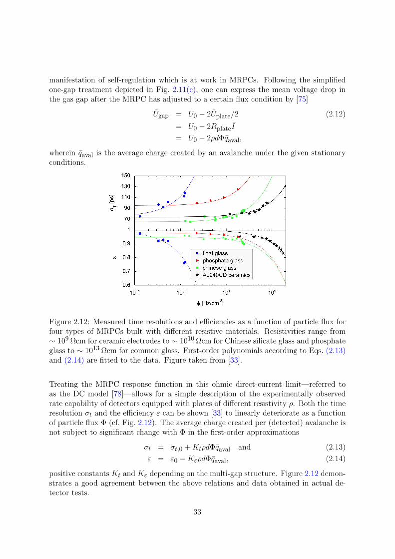
manifestation of self-regulation which is at work in MRPCs. Following the simplifiedone-gap treatment depicted in Fig. 2.11(c), one can express the mean voltage drop inthe gas gap after the MRPC has adjusted to a certain flux condition by [75]

Ugap = U0 − 2Uplate/2 (2.12)

= U0 − 2RplateI

= U0 − 2ρdΦqaval,

wherein qaval is the average charge created by an avalanche under the given stationaryconditions.

Figure 2.12: Measured time resolutions and efficiencies as a function of particle flux forfour types of MRPCs built with different resistive materials. Resistivities range from∼ 109 Ωcm for ceramic electrodes to ∼ 1010 Ωcm for Chinese silicate glass and phosphateglass to ∼ 1013 Ωcm for common glass. First-order polynomials according to Eqs. (2.13)and (2.14) are fitted to the data. Figure taken from [33].

Treating the MRPC response function in this ohmic direct-current limit—referred toas the DC model [78]—allows for a simple description of the experimentally observedrate capability of detectors equipped with plates of different resistivity ρ. Both the timeresolution σt and the efficiency ε can be shown [33] to linearly deteriorate as a functionof particle flux Φ (cf. Fig. 2.12). The average charge created per (detected) avalanche isnot subject to significant change with Φ in the first-order approximations

σt = σt,0 +KtρdΦqaval and (2.13)

ε = ε0 −KερdΦqaval, (2.14)

positive constants Kt and Kε depending on the multi-gap structure. Figure 2.12 demon-strates a good agreement between the above relations and data obtained in actual de-tector tests.

33

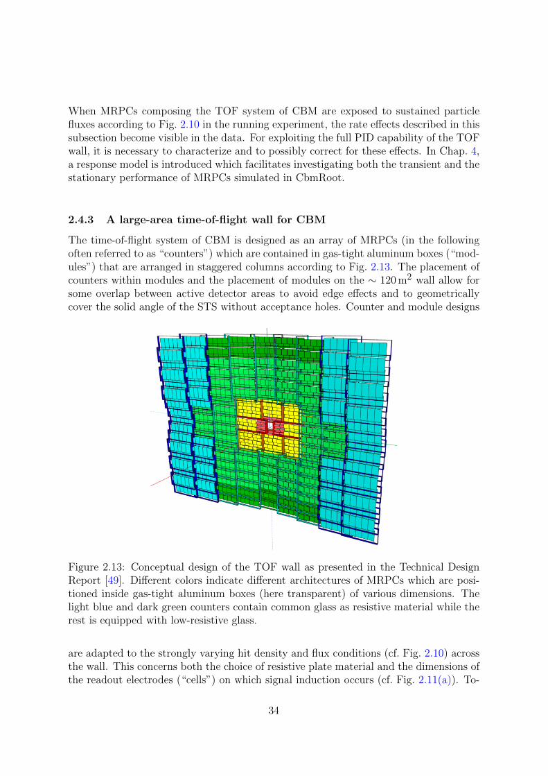
When MRPCs composing the TOF system of CBM are exposed to sustained particlefluxes according to Fig. 2.10 in the running experiment, the rate effects described in thissubsection become visible in the data. For exploiting the full PID capability of the TOFwall, it is necessary to characterize and to possibly correct for these effects. In Chap. 4,a response model is introduced which facilitates investigating both the transient and thestationary performance of MRPCs simulated in CbmRoot.

2.4.3 A large-area time-of-flight wall for CBM

The time-of-flight system of CBM is designed as an array of MRPCs (in the followingoften referred to as “counters”) which are contained in gas-tight aluminum boxes (“mod-ules”) that are arranged in staggered columns according to Fig. 2.13. The placement ofcounters within modules and the placement of modules on the ∼ 120 m2 wall allow forsome overlap between active detector areas to avoid edge effects and to geometricallycover the solid angle of the STS without acceptance holes. Counter and module designs

Figure 2.13: Conceptual design of the TOF wall as presented in the Technical DesignReport [49]. Different colors indicate different architectures of MRPCs which are posi-tioned inside gas-tight aluminum boxes (here transparent) of various dimensions. Thelight blue and dark green counters contain common glass as resistive material while therest is equipped with low-resistive glass.

are adapted to the strongly varying hit density and flux conditions (cf. Fig. 2.10) acrossthe wall. This concerns both the choice of resistive plate material and the dimensions ofthe readout electrodes (“cells”) on which signal induction occurs (cf. Fig. 2.11(a)). To-

34

wards the beam pipe where two particles are more likely to traverse the detector closelyin time and space, much higher cell granularities are required than at the periphery ofthe wall. An interference of two or more signals induced by different primary particleson the same cell complicates the matching of STS tracks with (distorted) TOF hits. Anoccupancy criterion of < 5 % for each readout cell in the TOF system serves as a pointof orientation for this design aspect. The counter size consequently shrinks with the sizeof the printed circuit board (PCB) into which the readout electrodes are integrated.

Table 2.1: Differences in design of MRPCs constituting different regions of the TOF wallas proposed in [49]. Naming conventions and specifications given in this table representa provisional point of reference for counter design and have partially been subject tomodifications.

MRPC1 MRPC2 MRPC3a MRPC3b MRPC4

color in Fig. 2.13 red yellow light green dark green light blue

resistive plates [#] 12 12 9 9 9

resistivity ρ [Ωcm] O(1010) O(1010) O(1010) O(1012) O(1012)

plate thickness d [µm] 700 700 700 500 500

plate surface [mm2] 320× 100 320× 200 330× 280 330× 280 330× 540

gas gaps [#] 10 10 8 8 8

gap width g [µm] 140 140 220 220 220

readout cells [#] 64 64 32 32 32

cell length [mm] 100 200 270 270 530

cell width [mm] 2.18 2.18 7 7 7

cell spacing [mm] 2.54 2.54 3 3 3

cell pitch [mm] 4.72 4.72 10 10 10

cell granularity [cm2] 4.7 9.4 27 27 53

active area [mm2] 302× 100 302× 200 320× 270 320× 270 320× 530

Table 2.1 summarizes the different MRPC designs for the outer TOF wall (MRPC3a,MRPC3b, and MRPC4) where particle fluxes are assumed to not exceed 8 kHz/cm2 andthe inner TOF wall (MRPC1 and MRPC2) where fluxes range from 8 to 25 kHz/cm2 [48].Except for the MRPC3a design which relies on low-resistive silicate glass developedin China [79] (therefore sometimes referred to as “Chinese” glass), the outer wall isequipped with common glass. The inner wall, in contrast, is entirely based on low-resistive glass plates due to the higher flux constraints. Regarding cell granularity, thedifference between the innermost MRPC1 counters and the outermost MRPC4 coun-ters corresponds to an order of magnitude. Architecture-wise, MRPC1 and MRPC2 areconstructed in a double-stack configuration, i.e. an intermediate layer of high-voltageelectrodes would effectively divide the single stack shown in Fig. 2.11(a) into two stacksadjacent to each other. This halves the high voltage which needs to be applied to create

35

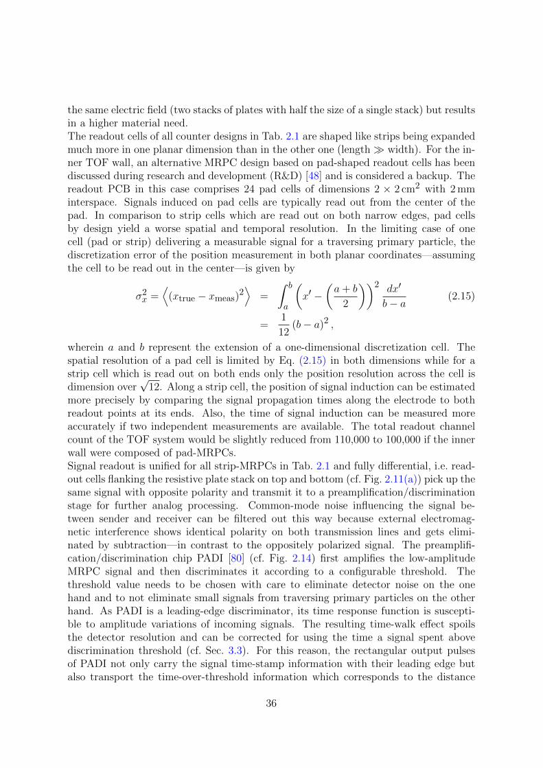
the same electric field (two stacks of plates with half the size of a single stack) but resultsin a higher material need.The readout cells of all counter designs in Tab. 2.1 are shaped like strips being expandedmuch more in one planar dimension than in the other one (length width). For the in-ner TOF wall, an alternative MRPC design based on pad-shaped readout cells has beendiscussed during research and development (R&D) [48] and is considered a backup. Thereadout PCB in this case comprises 24 pad cells of dimensions 2 × 2 cm2 with 2 mminterspace. Signals induced on pad cells are typically read out from the center of thepad. In comparison to strip cells which are read out on both narrow edges, pad cellsby design yield a worse spatial and temporal resolution. In the limiting case of onecell (pad or strip) delivering a measurable signal for a traversing primary particle, thediscretization error of the position measurement in both planar coordinates—assumingthe cell to be read out in the center—is given by

σ2x =

⟨(xtrue − xmeas)

2⟩

=

∫ b

a

(x′ −

(a+ b

2

))2 dx′

b− a(2.15)

=1

12(b− a)2 ,

wherein a and b represent the extension of a one-dimensional discretization cell. Thespatial resolution of a pad cell is limited by Eq. (2.15) in both dimensions while for astrip cell which is read out on both ends only the position resolution across the cell isdimension over

√12. Along a strip cell, the position of signal induction can be estimated

more precisely by comparing the signal propagation times along the electrode to bothreadout points at its ends. Also, the time of signal induction can be measured moreaccurately if two independent measurements are available. The total readout channelcount of the TOF system would be slightly reduced from 110,000 to 100,000 if the innerwall were composed of pad-MRPCs.Signal readout is unified for all strip-MRPCs in Tab. 2.1 and fully differential, i.e. read-out cells flanking the resistive plate stack on top and bottom (cf. Fig. 2.11(a)) pick up thesame signal with opposite polarity and transmit it to a preamplification/discriminationstage for further analog processing. Common-mode noise influencing the signal be-tween sender and receiver can be filtered out this way because external electromag-netic interference shows identical polarity on both transmission lines and gets elimi-nated by subtraction—in contrast to the oppositely polarized signal. The preamplifi-cation/discrimination chip PADI [80] (cf. Fig. 2.14) first amplifies the low-amplitudeMRPC signal and then discriminates it according to a configurable threshold. Thethreshold value needs to be chosen with care to eliminate detector noise on the onehand and to not eliminate small signals from traversing primary particles on the otherhand. As PADI is a leading-edge discriminator, its time response function is suscepti-ble to amplitude variations of incoming signals. The resulting time-walk effect spoilsthe detector resolution and can be corrected for using the time a signal spent abovediscrimination threshold (cf. Sec. 3.3). For this reason, the rectangular output pulsesof PADI not only carry the signal time-stamp information with their leading edge butalso transport the time-over-threshold information which corresponds to the distance

36

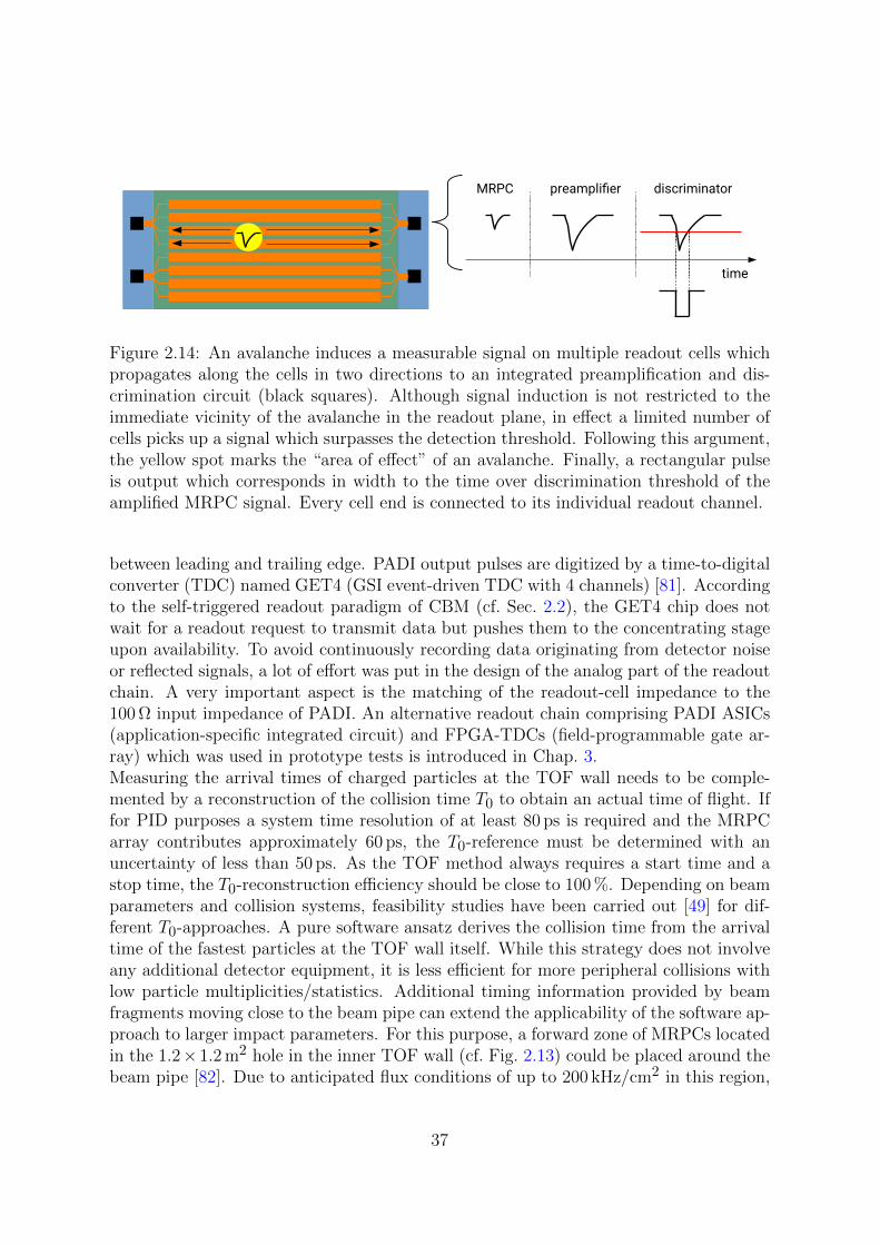
time

MRPC preamplifier discriminator

Figure 2.14: An avalanche induces a measurable signal on multiple readout cells whichpropagates along the cells in two directions to an integrated preamplification and dis-crimination circuit (black squares). Although signal induction is not restricted to theimmediate vicinity of the avalanche in the readout plane, in effect a limited number ofcells picks up a signal which surpasses the detection threshold. Following this argument,the yellow spot marks the “area of effect” of an avalanche. Finally, a rectangular pulseis output which corresponds in width to the time over discrimination threshold of theamplified MRPC signal. Every cell end is connected to its individual readout channel.

between leading and trailing edge. PADI output pulses are digitized by a time-to-digitalconverter (TDC) named GET4 (GSI event-driven TDC with 4 channels) [81]. Accordingto the self-triggered readout paradigm of CBM (cf. Sec. 2.2), the GET4 chip does notwait for a readout request to transmit data but pushes them to the concentrating stageupon availability. To avoid continuously recording data originating from detector noiseor reflected signals, a lot of effort was put in the design of the analog part of the readoutchain. A very important aspect is the matching of the readout-cell impedance to the100 Ω input impedance of PADI. An alternative readout chain comprising PADI ASICs(application-specific integrated circuit) and FPGA-TDCs (field-programmable gate ar-ray) which was used in prototype tests is introduced in Chap. 3.Measuring the arrival times of charged particles at the TOF wall needs to be comple-mented by a reconstruction of the collision time T0 to obtain an actual time of flight. Iffor PID purposes a system time resolution of at least 80 ps is required and the MRPCarray contributes approximately 60 ps, the T0-reference must be determined with anuncertainty of less than 50 ps. As the TOF method always requires a start time and astop time, the T0-reconstruction efficiency should be close to 100 %. Depending on beamparameters and collision systems, feasibility studies have been carried out [49] for dif-ferent T0-approaches. A pure software ansatz derives the collision time from the arrivaltime of the fastest particles at the TOF wall itself. While this strategy does not involveany additional detector equipment, it is less efficient for more peripheral collisions withlow particle multiplicities/statistics. Additional timing information provided by beamfragments moving close to the beam pipe can extend the applicability of the software ap-proach to larger impact parameters. For this purpose, a forward zone of MRPCs locatedin the 1.2× 1.2 m2 hole in the inner TOF wall (cf. Fig. 2.13) could be placed around thebeam pipe [82]. Due to anticipated flux conditions of up to 200 kHz/cm2 in this region,

37

Si3N4/SiC ceramics (ρ ∼ 109 Ωcm) are considered as resistive plate material. IndividualMRPCs for the proposed Beam Fragmentation T0 Counter (BFTC) have a triple-stackstructure with a surface of 2 × 2 cm2 and two gas gaps of 250µm per stack. A thirdoption for collision-time reconstruction is an explicit diamond start detector placed inbeam ahead of the target in the vacuum of the beam pipe. Despite of the low materialbudget of 300µm and 50µm, respectively, for detecting beams of protons/light nucleiand heavy ions, the interaction probability of the beam with the start detector stillamounts to 0.4 % which can—at high beam intensities—impose a significant additionalload on the CBM experiment. In this scenario, the foregoing methods are preferable.

38

CHAPTER 3

MRPC PROTOTYPE TESTS WITH HEAVY IONS

During research and development (R&D) of MRPC prototypes adapted in design tothe different flux regions of the future CBM time-of-flight wall (cf. Tab. 2.1), the TOFworking group conducted numerous irradiation tests at various test-beam facilities. Full-surface illuminations of large-area counters are feasible only with collision secondariesof accelerated heavy ions impinging on a fixed target which is mounted downstream ofthe test setup, allowing for higher intensities to be achieved than with two collidingion beams. In 2014 and in 2015, two such test-beam experiments were carried outeach year, first at GSI/SIS18 (in April and in October 2014) and then at CERN/SPS(in February/March and in November 2015), with different prototypes participatingand under varying experimental conditions, depending on the relative positioning ofcounters in the setup and on available ion species and beam intensities [83–89]. Forsuccessful data taking, a reliable data acquisition (DAQ) system is essential which wasrealized with conventionally hardware-triggered FPGA (field-programmable gate array)boards of the TRB3 (trigger and readout board) family [90]—customized to the needsof CBM TOF—in the aforementioned test-beam campaign, representing an importantfocus of this work. A stable version of the novel self-(respectively software-)triggeredDAQ concept of the future CBM experiment (cf. Fig. 2.3) which is gradually completed inthe ongoing mCBM experiment (see Sec. 5.4) was not available for counter readout at thetime. The hardware-triggered readout chain implemented for test-beam measurementsat GSI and CERN continues to be used for quality control (QC) in mass production ofMRPC3a [91] and MRPC3b [92] final counter designs with cosmic irradiation. The firstproduction badges of these counter types are deployed for end-cap time-of-flight (eTOF)measurements in the STAR experiment during phase II of the Beam Energy Scan (BES-II) at BNL/RHIC [93] and constitute the mTOF subsystem of the mCBM experimentat GSI/SIS18 [35], both activities being part of the intermediary FAIR Phase-0 researchprogram towards Day-1 experiments at the completed FAIR facility.In this chapter, the counter setup installed for the data-taking period at CERN/SPS inMarch 2015 and the particle-flux and multi-hit conditions which it was exposed to aredescribed in detail in Sec. 3.1. The latter are estimated by means of a dedicated MonteCarlo study developed in this work. Corresponding experimental data are suited for acomparison with simulated results presented in Chap. 5. The dual operation of the DAQchain based on a both periodically and physics-triggered TrbNet [94] (the communicationprotocol implemented between FPGAs) is outlined in Sec. 3.2. Finally, Sec. 3.3 coversthe calibration of raw detector messages and the reconstruction of correlations betweenthem in time and space, a process called cluster building. Within the scope of thiswork, a particular effort was made concerning the synchronization of prototype datameasured by 512 individual readout channels which were distributed over 20 time-to-digital converters (TDCs).

39

3.1 Test-beam setup at CERN/SPS in March 2015

3.1.1 Detection instruments and geometry

Registered as test-beam users at CERN under the abbreviation RE21/CBM (Recog-nized Experiment) since 2011, CBM TOF and TRD working groups successfully appliedfor participation—for a seven-day period—in a beam momentum scan of Ar18+ ions ona scandium fixed target conducted by the NA61/SHINE experiment [95] in the CERNNorth Area (NA) between February and April 2015. From Thursday, February 26, 08:00a.m. to Thursday, March 5, 08:00 a.m. collision data from 13 and 19 A GeV/c argon ionsaccelerated by the SPS impinging on a variable-size lead target were taken in a dedicatedconcrete cave—shown in Fig. 3.1—on the H4 beam line which runs parallel to the H2beam line at which NA61/SHINE is located.

Figure 3.1: Aerial view of the test-beam setup installation in the PPE134 (ParticlePhysics Experiment) zone of EHN1 (Experimental Hall North) at CERN in a dedicatedconcrete cave (dimensions: 2.6–4.2 m wide (x), 2.4 m high (y), and 8.0 m long (z)) down-stream the GOLIATH dipole magnet (left image). The beam enters the roofed cavethrough a beam pipe under vacuum at 1.26 m above the cave floor and—upon exitingthe beam pipe—hits a lead target (not visible) to produce a spray of collision secondariesto irradiate the setup (right image). Photographs by courtesy of D. Emschermann.

The construction of a temporary CBM cave in the PPE134 zone from shielding concreteagainst collision products was necessary to operate the test-beam setup under particlefluxes on the order of kHz/cm2 which would not be possible in an open experimental halldue to radiation protection. Different counters under test were mounted in their respec-tive aluminum gas boxes on an aluminum frame (cf. Fig. 3.1, left image), arranged in anupper branch more distant to the beam (z-)axis (exposed to smaller particle fluxes) andin a lower branch closer to the axis (exposed to higher particle fluxes). Results obtainedfor counters on the lower branch, exclusively equipped with low-resistive glass, are pub-lished in [84]. This work focuses on the upper branch of the setup, consisting of four

40

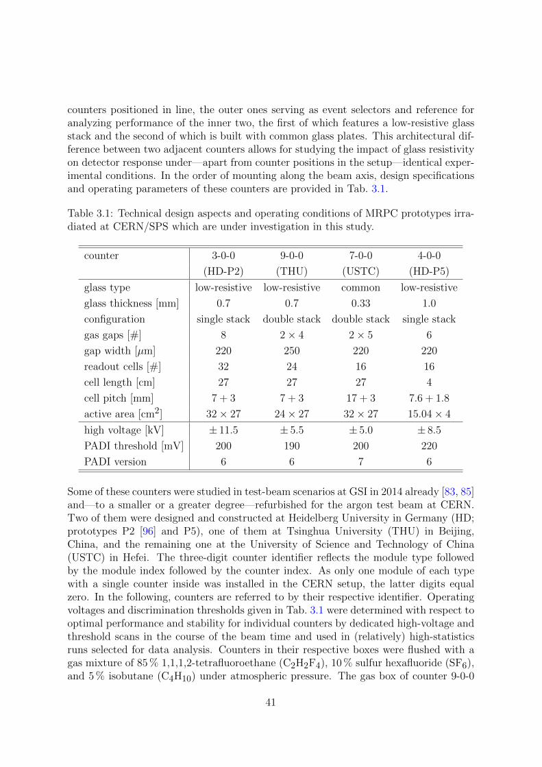
counters positioned in line, the outer ones serving as event selectors and reference foranalyzing performance of the inner two, the first of which features a low-resistive glassstack and the second of which is built with common glass plates. This architectural dif-ference between two adjacent counters allows for studying the impact of glass resistivityon detector response under—apart from counter positions in the setup—identical exper-imental conditions. In the order of mounting along the beam axis, design specificationsand operating parameters of these counters are provided in Tab. 3.1.

Table 3.1: Technical design aspects and operating conditions of MRPC prototypes irra-diated at CERN/SPS which are under investigation in this study.

counter 3-0-0 9-0-0 7-0-0 4-0-0

(HD-P2) (THU) (USTC) (HD-P5)

glass type low-resistive low-resistive common low-resistive

glass thickness [mm] 0.7 0.7 0.33 1.0

configuration single stack double stack double stack single stack

gas gaps [#] 8 2× 4 2× 5 6

gap width [µm] 220 250 220 220

readout cells [#] 32 24 16 16

cell length [cm] 27 27 27 4

cell pitch [mm] 7 + 3 7 + 3 17 + 3 7.6 + 1.8

active area [cm2] 32× 27 24× 27 32× 27 15.04× 4

high voltage [kV] ± 11.5 ± 5.5 ± 5.0 ± 8.5

PADI threshold [mV] 200 190 200 220

PADI version 6 6 7 6

Some of these counters were studied in test-beam scenarios at GSI in 2014 already [83, 85]and—to a smaller or a greater degree—refurbished for the argon test beam at CERN.Two of them were designed and constructed at Heidelberg University in Germany (HD;prototypes P2 [96] and P5), one of them at Tsinghua University (THU) in Beijing,China, and the remaining one at the University of Science and Technology of China(USTC) in Hefei. The three-digit counter identifier reflects the module type followedby the module index followed by the counter index. As only one module of each typewith a single counter inside was installed in the CERN setup, the latter digits equalzero. In the following, counters are referred to by their respective identifier. Operatingvoltages and discrimination thresholds given in Tab. 3.1 were determined with respect tooptimal performance and stability for individual counters by dedicated high-voltage andthreshold scans in the course of the beam time and used in (relatively) high-statisticsruns selected for data analysis. Counters in their respective boxes were flushed with agas mixture of 85 % 1,1,1,2-tetrafluoroethane (C2H2F4), 10 % sulfur hexafluoride (SF6),and 5 % isobutane (C4H10) under atmospheric pressure. The gas box of counter 9-0-0

41

Figure 3.2: Double-diamond detector located below the golden electrode layer on twostacked PCBs (printed circuit board), respectively, equipped with two PADI-8D chipseach (top left image). Open gas-tight aluminum box of counter 9-0-0 displaying theyellowish honeycomb support structure of the glass stack and two lines of PADI-6 add-onPCBs on opposing readout sides (top middle image). Stack of TRB3 data concentrators(top and bottom right images) cabled for operating a TrbNet DAQ network betweenFPGAs of the LatticeECP3 family (black packages) to read out a series of front-endTDC cards (bottom left image) digitizing PADI output signals. Photographs providedby GSI and by courtesy of Y. Wang (top middle) and D. Emschermann (top right).

without the top aluminum cover is shown in Fig. 3.2.Three and one centimeters ahead of the lead target, respectively, a double-diamonddetector is installed as a beam reference counter a signal on which is required for anypositive physics-trigger decision to be taken by the DAQ system. Additionally, it pro-vides a stable time reference for offset and velocity corrections in raw-data calibration(cf. Sec. 3.3) and—due to a lack of detector noise in the absence of beam—facilitates theestimation of event times in an ongoing spill of particles extracted from the acceleratorwith respect to the beginning of the spill (cf. Sec. 5.3). As time residuals between MR-PCs are considered in data analysis, the detector is not needed for T0-determination.The device used at CERN is the second version of a prototypical focal-plane detectorfor the Super-FRS (Superconducting FRagment Separator) at FAIR [97, 98], contribut-

42

ing time-of-flight information to the identification of exotic nuclear fragments which arestudied by NUSTAR. Both readout PCBs of the double-detector contain a pcCVD (poly-crystalline chemical vapor deposition) diamond of dimensions 20 mm× 20 mm× 0.3 mmwith Cr/Au layers deposited on each side by photolithography serving as electrodes, thetop side being segmented into 16 readout cells (pitch: 1 mm + 0.15 mm, length: 18 mm)and the bottom side acting as a planar ground pad (18.25 mm×18 mm). Cell orientationis horizontal on the first layer and vertical on the second layer. To not overload the DAQsystem with diamond data at beam intensities on the order of 107 Hz (cf. Sec. 3.1.2),no focusing effort was made to center the beam on the diamonds. Instead, the detectorwas positioned 1 cm above the nominal beam height and operated with the maximumavailable discrimination threshold for PADI-8D (−600 mV).For an independent estimation of particle fluxes in the setup, two Bicron BC-408 plasticscintillators of xyz-dimensions 8 cm× 2 cm× 1 cm and 11 cm× 4 cm× 2 cm, respectively,are positioned in front of (smaller unit) and behind (larger unit) the line of MRPCs(cf. Fig. 3.3). Two H2431-50 photomultiplier tube (PMT) assemblies each are attachedto scintillator edges on the longitudinal axis for generating measurable electrical signalsfrom scintillation light.

Figure 3.3: Visualization of the simplified test-beam setup described with TGeo vol-umes in ROOT (cf. Tab. 3.2). While the beam moves along the z-axis, it first crossesthe double-diamond detector right ahead of the point of origin on which the targetis centered. Reaction secondaries propagating through the setup eventually penetratethe glass stack of an MRPC (yellow) or a plastic scintillator (red). MRPC gas boxes(transparent teal) additionally contain rectangular readout PCBs (green).

For data analysis and simulations, component geometries of detection instruments inthe setup are—in a greatly simplified fashion—implemented in ROOT with the TGeogeometry modeler (cf. Fig. 3.3). The entire setup is described with rectangular mothervolumes containing rectangular daughter volumes of different size and material, the topvolume in the hierarchy being a virtual cave filled with air composed of 78 % nitro-gen (N2), 21 % oxygen (O2), and 1 % argon (Ar), given in molar proportions. In thiscave volume, MRPC modules are placed according to actual positions at the experimen-

43

Table 3.2: Geometrical constraints of the MRPC test-beam setup complementingTab. 3.1 with respect to counter positioning and projected detection areas under testwith all four counters triggered by straight-line particle tracks (4xTRG). A TGeo visu-alization is provided in Fig. 3.3. (Side note: On grounds of historically grown geometricdescriptions of counters in software, TGeo active areas might negligibly deviate from thetechnical values stated in Tab. 3.1.)

counter 3-0-0 9-0-0 7-0-0 4-0-0

cell orientation horizontal horizontal horizontal vertical

TGeo active area [cm2] 32× 26.9 25× 26.7 32× 27 15.04× 4

860.8 667.5 864.0 60.2

counter x-center [cm] 0.0 2.8 −0.4 3.1

counter y-center [cm] 48.9 55.0 58.2 66.8

counter z-center [cm] 265.9 297.5 332.3 367.4

shortest time of flight [ns] 9.0 10.1 11.2 12.5

4xTRG projection area [cm2] 10.9× 2.9 12.2× 3.2 13.6× 3.6 15.04× 4

31.6 39.0 49.0 60.2

cells in projection area 14, 15, 16 9, 10, 11, 12 8, 9 0–15

tal site, slightly readjusted during data analysis based on measured spatial correlationsbetween counters. The outer volume of an MRPC module is a hollow gas box of module-dependent dimensions made of elemental aluminum with wall thicknesses of 0.1 cm alongcave-y and cave-z (beam axis) and of 0.5 cm along cave-x where the feed-through of elec-trical counter signals occurs in reality. The gas box is filled with a passive gas volume(85 % C2H2F4, 10 % SF6, and 5 % C4H10) which serves as mother volume to a stackof soda–lime–silica (common) glass plates (used in ROOT also for counters with low-resistive glass), composed of 73.5 % silicon dioxide (SiO2), 15.9 % sodium oxide (Na2O),and 10.6 % calcium oxide (CaO), interspaced with active gas-gap volumes. The dimen-sions of the gas gaps determine the active counter area (cf. Tab. 3.2). Counters witha double-stack configuration are modeled as single stacks, preserving the total numberof gas gaps but omitting the readout plane (and a glass plate) in the middle. Attachedto opposing sides of the glass stack, either along cave-x or along cave-y depending onthe respective orientation of readout cells, two volumes of elemental carbon represent-ing front-end electronic boards equipped with PADI chips contribute some additionalmaterial budget. As pick-up electrodes carrying readout cells above and below the glassstack are not implemented, the counter volume is logically divided into the correspondingnumber of strip-shaped cells, taking the pitch between real cells as the width of imme-diately adjacent virtual cells. The double-diamond detector is virtualized as two smallMRPC modules with active areas of 2 cm× 2 cm, respectively, each logically segmentedinto 16 readout cells. Situated ahead of the target, the detector does—except for some

44

rare combinations of scattering processes—not add material budget to trajectories ofcollision secondaries from the target volume which irradiate the counter setup. Treatingit as an MRPC in software allows for modeling its response function (cf. Chap. 4) in thesame way. A more accurate description is not required for data analysis in this workwhich concentrates on residuals between MRPCs. Finally, the two plastic scintillatorsin the setup are implemented as two blocks of hydrocarbon with an H/C atomic ratioof 1, positioned in the virtual cave in front of counter 3-0-0 and behind counter 4-0-0.

x

y

z

cave coordinateslocal coordinates A local coordinates B

x‘(x)

y‘(y) x‘(y)

cell side/ index

7 … 0

+

–

cell index/ side

– +

7

...

0 y‘(-x)

Figure 3.4: Comparison of cave and local counter coordinate systems for vertical (A; leftdrawing) and horizontal (B; right drawing) cell orientations. While local cell indexing inboth cases runs along global x- (A) or global y-coordinates (B), respectively, the cell endmarked with a plus sign is directed towards negative global x in case B (towards positiveglobal y in case A in contrast) as the latter orientation (B) results from a clock-wiserotation by 90 of the former (A). The point of origin of local coordinates is the centerof the glass stack. Note that in the TGeo representation—in contrast to this sketchaiming at a clear and simple view—no gaps exist between virtual cells, the cell widthcorresponding to the cell pitch.

The total active detection volume, i.e. the entirety of gas gaps interspaced with glassplates, is centered about the point of origin in xyz of the local coordinate frame of thecounter. The volume in the middle of this stack which is either a glass plate (if thenumber of gaps is even) or a gas gap (in case of an odd gap number) contains the localorigin in z and serves as a reference plane for coordinate transformations between thelocal counter frame and the global cave frame (cf. Fig. 3.4). To any hit reconstructedon the counter, a local z-coordinate of 0 is assigned. If the readout cell indexed with ifires, the reconstructed hit is positioned at the (pitch) center of cell i on the x-axis ofthe local coordinate system,

xcenter (i) = (i−Ncells/2 + 1/2)xpitch, (3.1)

i.e. logical cells with pitch xpitch are indexed along local x, starting from cell 0 in thelower negative x-range and ending with cell Ncells − 1 in the upper positive x-range,constrained by the extension of the active area in this dimension. Reversely, the spatialpassage of a simulated Monte Carlo track through the active counter volume—an average

45

over positions in all gas gaps involved—is interpreted in local x as a hit on cell

i (x) =⌊x/xpitch +Ncells/2

⌋. (3.2)

Hit coordinates in local y are derived from half the difference of digitized signal arrivaltimes on opposing cell ends,

y = 1/2(t− − t+

)vsignal, (3.3)

multiplied with the measured propagation velocity vsignal of signals on the pick-up elec-trodes. Signal induction closer to the cell end marked negative in Fig. 3.4 results in anegative local y-coordinate for the corresponding hit (t− < t+) while a positive localy-coordinate results from a signal generated closer to the positive cell end (t− > t+).

3.1.2 Particle flux and spill structure

To assess the high-rate performance of counters in a test-beam environment, a homoge-neous flux—especially in time—of particles on the respective surfaces over a sustainedperiod of a few seconds is a desired condition concerning reproducibility of measuredresults both in subsequent experiments and in simulations with mathematical modelsthat are not limited to a very specific scenario. As the argon test beam at CERN/SPSin early 2015 marked the beginning of efforts by the CBM-TOF working group to testdetector prototypes under the highest possible load at this location, details regarding theavailable beam intensity in the dedicated concrete cave (cf. Fig. 3.1) and the temporalhomogeneity of the beam in spill had to be learned during this beam time. Originally,incident particle fluxes from the beam colliding with a variable-size lead target of upto 25 kHz/cm2 were aimed at to evaluate the full potential of prototypes for the innerTOF wall (cf. Sec. 2.4.3) which were mounted in the lower branch of the setup. Due toconstraints imposed by radiation protection, however, the setup could not be operatedunder stable conditions above 2.3 kHz/cm2 in the upper branch (5.5 kHz/cm2 in thelower branch), deduced from rate measurements with plastic scintillators, i.e. stronglydepending on their respective position. In Fig. 3.5, the particle flux on the two scintil-lators in front of and behind the upper line of counters (cf. Fig. 3.3) is shown during astable run with final operating parameters in the evening of March 4. Remarkably, thethree flux patterns in both plots which each represent an accelerator spill all start with ahuge spike, at least three times higher in flux than the subsequent regular spill, providedthat PMTs were able to follow, i.e. no saturation occurred. Owing to the intentionallysmall readout frequency of scaler registers for diamond, MRPC, and PMT signals ona set of VULOM (VME Universal Logic Module) boards by an MBS (Multi BranchSystem) [99] running in parallel to the main TrbNet-based DAQ system, the width ofthe initial spike in beam intensity and the microscopic intensity structure of the regularspill are not resolved in Fig. 3.5.With a periodically triggered TrbNet readout, the distribution of digital detector mes-sages (“digis”) on a continuous experiment time axis shows the SPS spill structure (and

46

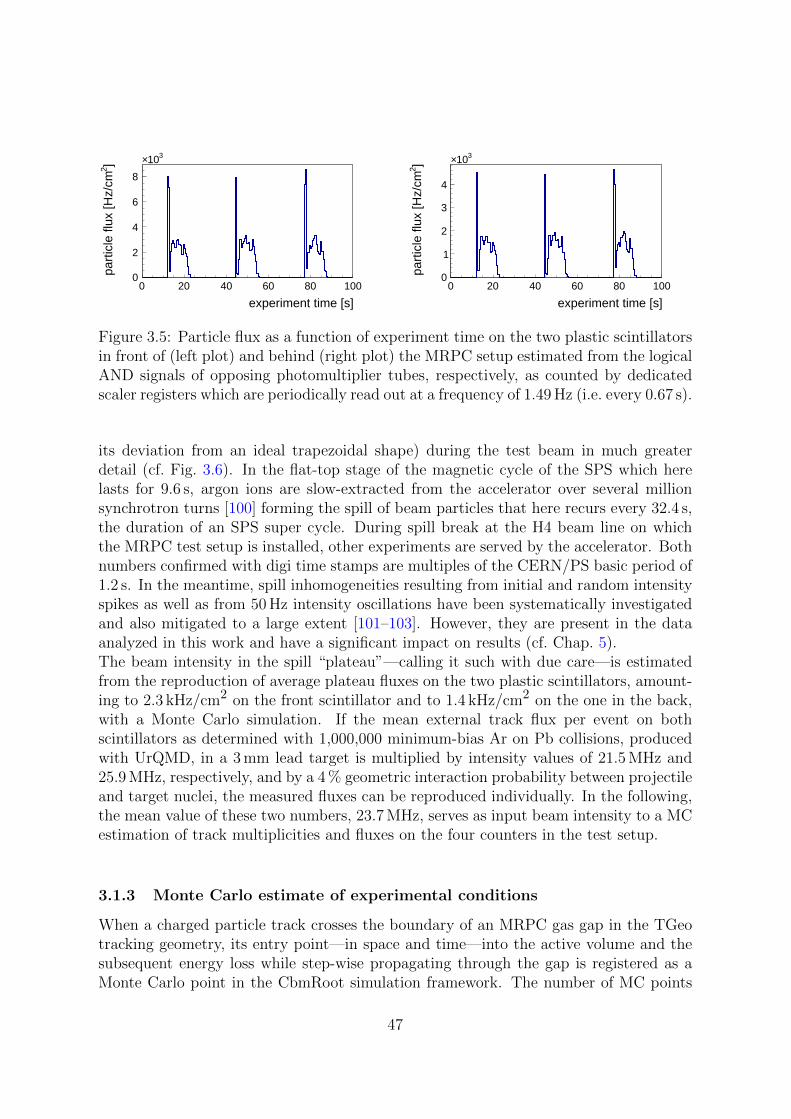
0 20 40 60 80 100

experiment time [s]

0

2

4

6

8

310×]2 p

artic

le fl

ux [H

z/cm

0 20 40 60 80 100

experiment time [s]

0

1

2

3

4

310×]2 p

artic

le fl

ux [H

z/cm

Figure 3.5: Particle flux as a function of experiment time on the two plastic scintillatorsin front of (left plot) and behind (right plot) the MRPC setup estimated from the logicalAND signals of opposing photomultiplier tubes, respectively, as counted by dedicatedscaler registers which are periodically read out at a frequency of 1.49 Hz (i.e. every 0.67 s).

its deviation from an ideal trapezoidal shape) during the test beam in much greaterdetail (cf. Fig. 3.6). In the flat-top stage of the magnetic cycle of the SPS which herelasts for 9.6 s, argon ions are slow-extracted from the accelerator over several millionsynchrotron turns [100] forming the spill of beam particles that here recurs every 32.4 s,the duration of an SPS super cycle. During spill break at the H4 beam line on whichthe MRPC test setup is installed, other experiments are served by the accelerator. Bothnumbers confirmed with digi time stamps are multiples of the CERN/PS basic period of1.2 s. In the meantime, spill inhomogeneities resulting from initial and random intensityspikes as well as from 50 Hz intensity oscillations have been systematically investigatedand also mitigated to a large extent [101–103]. However, they are present in the dataanalyzed in this work and have a significant impact on results (cf. Chap. 5).The beam intensity in the spill “plateau”—calling it such with due care—is estimatedfrom the reproduction of average plateau fluxes on the two plastic scintillators, amount-ing to 2.3 kHz/cm2 on the front scintillator and to 1.4 kHz/cm2 on the one in the back,with a Monte Carlo simulation. If the mean external track flux per event on bothscintillators as determined with 1,000,000 minimum-bias Ar on Pb collisions, producedwith UrQMD, in a 3 mm lead target is multiplied by intensity values of 21.5 MHz and25.9 MHz, respectively, and by a 4 % geometric interaction probability between projectileand target nuclei, the measured fluxes can be reproduced individually. In the following,the mean value of these two numbers, 23.7 MHz, serves as input beam intensity to a MCestimation of track multiplicities and fluxes on the four counters in the test setup.

3.1.3 Monte Carlo estimate of experimental conditions

When a charged particle track crosses the boundary of an MRPC gas gap in the TGeotracking geometry, its entry point—in space and time—into the active volume and thesubsequent energy loss while step-wise propagating through the gap is registered as aMonte Carlo point in the CbmRoot simulation framework. The number of MC points

47

78 80 82 84 86 88

experiment time [s]

0

0.5

1

1.5

2

310×

dia

mon

d di

gis

/ ms

[]

78 78.5 79 79.5 80

experiment time [s]

1

10

210

310

dia

mon

d di

gis

/ ms

[]

78 78.5 79 79.5 80

experiment time [s]

1

10

210

310

MR

PC

dig

is /

ms

[]

Figure 3.6: Typical spill structure and length during the test beam at SPS visualized bydigital diamond-detector messages per ms experiment time (upper plot). Zoomed viewof the spill start showing a roughly 100 ms wide initial spike of—due to fragmentaryrecording—unknown intensity less than 0.5 s ahead of the actual spill (lower two plots;cf. Fig. 3.5). A subspill intensity pattern of 50 Hz is clearly visible. The double-diamonddetector does not show any off-spill noise (middle plot) in contrast to counter 9-0-0, forinstance (lower plot). Holes appearing on the experiment time axis result from data lossin the readout system and in the event builder, respectively.

per counter produced for a track can amount to the total number of gaps if a tracktraverses the entire counter volume from top to bottom or even be limited to 1 if, forinstance, a daughter track is created during propagation of a mother track through theglass plate in front of the last gap in the stack. Also, if a track decays in the countervolume or is kinetically stopped, the number of MC points is smaller than the gapnumber. In the Monte Carlo formalism, a track is considered geometrically detectedby a counter if any corresponding MC point exists. As a level of detail at which entry

48

points and energy losses are stored for individual gas gaps is not required for simulationpurposes in this work, a single MC point per track per counter is created based onaverage coordinates in position and time and on accumulated energy loss in all gapscrossed. Regarding particle flux on a counter surface, external tracks originating outsidethe respective module, i.e. the gas-box volume, need to be distinguished from internaltracks which result from interactions of an external track with module material or fromparticle decays inside the module. The former are counted towards (external) particleflux, the latter are considered part of the detector response. External tracks—whethercharged or uncharged—are taken into account only once, independent of the numberof internal descendants, even if no direct MC point exists for them, as long as at leastone MC point is created for an internal daughter track. For the first station in the lineof MRPCs, counter 3-0-0, creation mechanisms of both the external and the internalparticle cocktail leaving traces in the detector are summarized in Fig. 3.7.

0.00 0.00 0.01

0.01

0.02

0.00 0.00 0.02

0.01 0.00 0.02 0.00

0.00 0.09

0.01 0.00 0.09

0.02 0.02 0.16

0.01 0.02 0.20

0.01 0.04 0.22

BREM DRAY HADR DCAY PAIR PRIM

creation process []

-Κ+µ-µ+Κγ+e

-ep+π-π

ext

erna

l par

ticle

[]

0

0.05

0.1

0.15

0.2

0.02

0.04

0.00 0.05

0.00 0.05

0.01 0.12

0.00 0.17

0.00 0.03 0.12 0.39

DCAY COMP PAIR HADR DRAY

creation process []

t

d

+π

-π

+e

p

-e in

tern

al p

artic

le []

0

0.1

0.2

0.3

Figure 3.7: Production processes of externally (left plot) and internally (right plot)created particles which traverse an active detector volume of counter 3-0-0. The formerset—in contrast to the latter—comprises also uncharged tracks a charged descendant ofwhich is detected. External particles are created either in the target (86.8 %) or in air(12.8 %) while internal particles usually originate from a glass plate (85.9 %) or from thealuminum box (12.6 %). Normalized contributions up to a limit of 0.5 % are not shown.Process names are abbreviated in the following way: bremsstrahlung (BREM), Comptonscattering (COMP), particle decay (DCAY), delta-ray production (DRAY), hadronicinteraction (HADR), pair production (PAIR), and collision-seed primaries (PRIM).

A share of internal tracks from counter 3-0-0 contributes to the respective externalparticle flux on the three rear modules. Actually, each module in the row successivelyadds rate to subsequent modules, mainly by interactions in the aluminum box or thesoda–lime–silica glass stack which have similar material properties. The main source ofelectron–positron pairs created either in the target material or inside module aluminumor glass, respectively, are decay gammas from primary π0 → γγ. Due to the shortlifetime of neutral pions (cτ = 0.2µm at p = 1 GeV/c), these decays happen exclusivelyin the dz = 3 mm thick lead target wherein a photon with sufficiently high energy has achance of

P (0 ≤ Z ≤ dz) = 1− exp

[−7

9

ρ

X0dz

](3.4)

49

to engage in pair production, Z being a random position variable, ρ the material density,and X0 its radiation length. In numbers (material properties taken from [29]), 34 % ofπ0-decay gammas are converted into an e+e−-pair in the target while surviving gam-mas irradiating the line of modules have a probability to interact accordingly of 0.9 %in every 1 mm aluminum wall and of 0.5 % in every 0.7 mm glass plate in the line ofcounters—material contributions which sum up towards the rear end of the setup. Thepredominant creation mechanism of internal particles is delta-ray production in the glassstack.Events relevant to data analysis are those in which a combination of counters respondedto a straight-line track, ideally originating from the target volume. In the first stageof MRPC data calibration against a stable time reference, as provided by the diamonddetector, only the respective counter needs to have fired (which is reflected by a setof independent trigger conditions between the diamond and individual counters in theDAQ system). When calibrating on and finally analyzing correlations between selectorcounters and detectors under test, the entire line of counters is required to be triggered.In the following, Monte Carlo events corresponding to the former case (any counteris hit) are labeled with 1xTRG (abbr. for trigger) and events qualifying for the lattercase, comprising a target track crossing all four counters, are denoted with 4xTRG. Therespective counter areas which can geometrically be traversed by straight-line 4xTRGselector tracks match with the projections of the small reference counter 4-0-0 (locatedin the back) towards the point of origin onto the respective counter planes (cf. Tab. 3.2).This spatial corridor is reflected in the narrow phase-space acceptance of selector par-ticles (cf. Fig. 3.8). Among selector tracks, also a significant share of electron–positronpairs (20 %) can be found with trajectories that deviate—on average—more from thestraight-line ideal than trajectories of selector bulk hadrons (pions, kaons, and protons)because of deflections arising from multiple Coulomb scattering with nuclei in the track-ing material.

1− 0 1 2 3 4

[]lab

y

0

0.5

1

1.5

2

2.5

/(m

c) []

tp

1

10

210

310

0.00 0.01

0.00 0.03

0.00 0.10

0.00 0.10

0.00 0.01 0.20

0.01 0.01 0.25

0.01 0.01 0.27

DCAY HADR PAIR PRIM

creation process []

-Κ

+Κ

+e

-e

p

+π

-π

sel

ecto

r pa

rtic

le []

0

0.1

0.2

Figure 3.8: Phase space populated by Monte Carlo selector tracks which originate fromthe target volume and traverse all four counters (4xTRG) in the setup. The bluecurve corresponds to the 10.3 central polar angle of the last counter in line (left plot;cf. Fig. 2.7). Particle type and creation mechanism of selector tracks in the target (rightplot; for abbreviations see caption of Fig. 3.7). Normalized contributions up to a limitof 0.5 % are not shown.

50

Table 3.3: Monte Carlo track multiplicities (MUL), fluxes, and cell occupancies on thefour MRPCs in the setup under various aspects. Note that the sum of mean exter-nal and internal charged track multiplicities slightly exceeds the mean multiplicity ofMonte Carlo points as an external track triggering a response in an MRPC module bydescendants might not have traversed an active detection volume itself.

counter 3-0-0 9-0-0 7-0-0 4-0-0

external charged track MUL 1.592 1.030 1.197 0.068

external uncharged track MUL 0.058 0.038 0.032 0.003

total external track MUL 1.650 1.068 1.229 0.071

total external track flux [kHz/cm2] 1.817 1.517 1.348 1.119

total external track MUL (1xTRG) 3.040 1.968 2.264 0.131

total external track MUL (4xTRG) 4.821 3.526 3.897 1.145

selector track MUL (4xTRG) 0.045 0.045 0.045 0.045

internal charged track MUL 0.354 0.221 0.177 0.014

internal/external track MUL ratio [%] 17.7 17.1 12.7 16.5

Monte Carlo point MUL 1.938 1.246 1.369 0.082

Monte Carlo point flux [kHz/cm2] 2.135 1.770 1.502 1.290

readout-cell occupancy [%] 4.8 4.1 6.8 0.4

readout-cell occupancy (1xTRG) [%] 8.9 7.6 12.5 0.8

readout-cell multi-track prob. [%] 6.3 7.1 11.6 2.7

Track multiplicities on counters vary depending on the trigger condition, i.e. the event-selection criterion, in place. Table 3.3 summarizes mean multiplicities of different tracktypes. The argon-on-lead test beam analyzed in this work is a multi-track (multi-hit)scenario with an interfering counter response to individual tracks. In 4xTRG events, theaverage external track multiplicity on large-area prototypes is greater than 3 which neces-sitates a dedicated evaluation of multi-hit effects during data analysis (cf. Sec. 5.2). Meanparticle fluxes on the counters vary depending on the respective position in the setup,ranging from 1.8 kHz/cm2 on 3-0-0 in the front to 1.1 kHz/cm2 on 4-0-0 in the back. Forsix external tracks, about one internal (charged) track is created in a module, varyingwith material budget. The extraordinary behavior of counter 7-0-0 is linked to its con-struction with thin glass plates (0.33 mm in thickness compared to 0.7 mm and 1.0 mm,respectively). Concerning simulations with an active particle memory (cf. Sec. 4.2), thetotal number of Monte Carlo points to be expected in the run—whether of external orof internal origin—is an important quantity for estimating computation times.Data rates to be transported by a triggered DAQ system can be anticipated—and thereadout be configured accordingly—with reliable numbers on trigger frequency and onreadout-cell occupancy which—on a Monte Carlo level—corresponds to the share ofevents (under a given trigger condition) in which the volume of a virtual cell is traversed

51

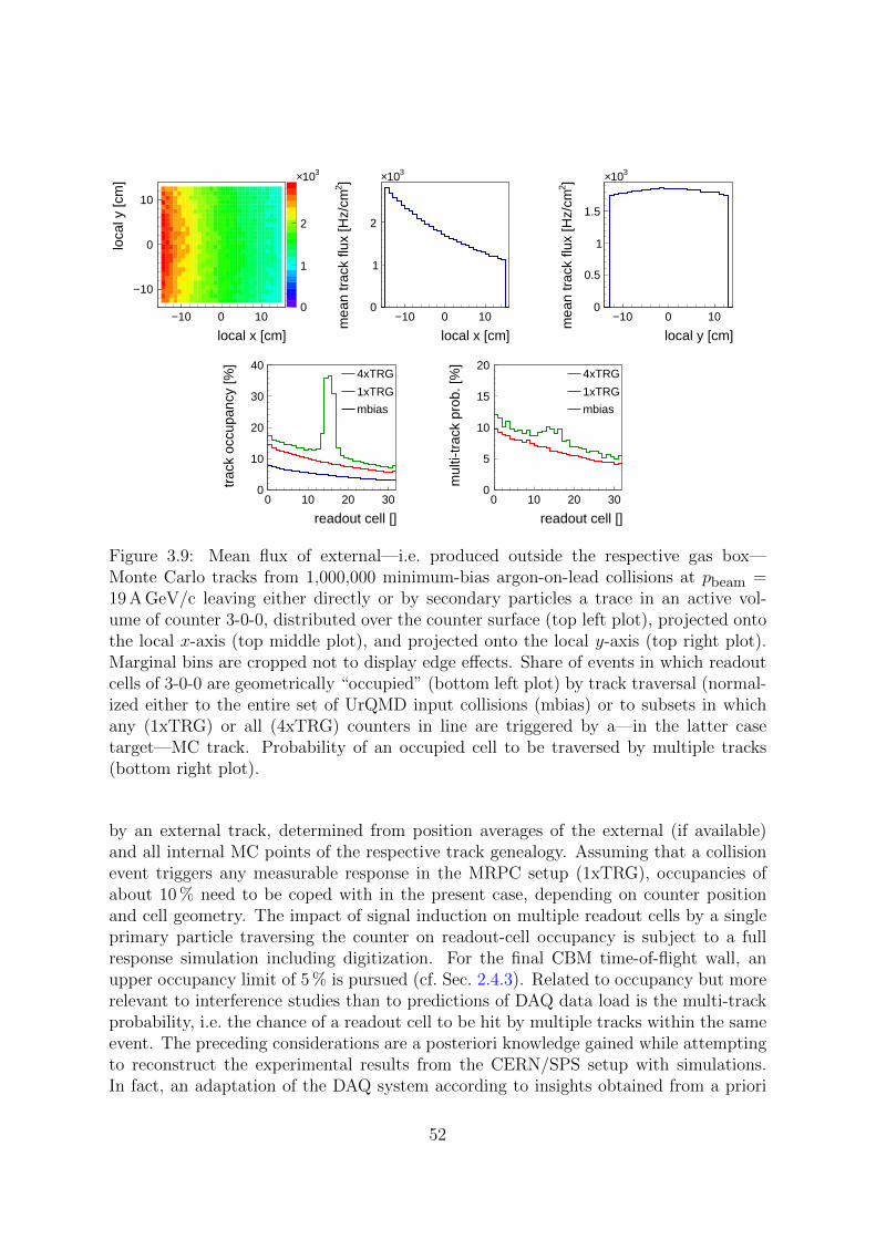
10− 0 10

local x [cm]

10−

0

10

loca

l y [c

m]

0

1

2

310×

10− 0 10

local x [cm]

0

1

2

310×]2 m

ean

trac

k flu

x [H

z/cm

10− 0 10

local y [cm]

0

0.5

1

1.5

310×]2 m

ean

trac

k flu

x [H

z/cm

0 10 20 30

readout cell []

0

10

20

30

40

trac

k oc

cupa

ncy

[%]

4xTRG

1xTRG

mbias

0 10 20 30

readout cell []

0

5

10

15

20

mul

ti-tr

ack

prob

. [%

]

4xTRG

1xTRG

mbias

Figure 3.9: Mean flux of external—i.e. produced outside the respective gas box—Monte Carlo tracks from 1,000,000 minimum-bias argon-on-lead collisions at pbeam =19 A GeV/c leaving either directly or by secondary particles a trace in an active vol-ume of counter 3-0-0, distributed over the counter surface (top left plot), projected ontothe local x-axis (top middle plot), and projected onto the local y-axis (top right plot).Marginal bins are cropped not to display edge effects. Share of events in which readoutcells of 3-0-0 are geometrically “occupied” (bottom left plot) by track traversal (normal-ized either to the entire set of UrQMD input collisions (mbias) or to subsets in whichany (1xTRG) or all (4xTRG) counters in line are triggered by a—in the latter casetarget—MC track. Probability of an occupied cell to be traversed by multiple tracks(bottom right plot).

by an external track, determined from position averages of the external (if available)and all internal MC points of the respective track genealogy. Assuming that a collisionevent triggers any measurable response in the MRPC setup (1xTRG), occupancies ofabout 10 % need to be coped with in the present case, depending on counter positionand cell geometry. The impact of signal induction on multiple readout cells by a singleprimary particle traversing the counter on readout-cell occupancy is subject to a fullresponse simulation including digitization. For the final CBM time-of-flight wall, anupper occupancy limit of 5 % is pursued (cf. Sec. 2.4.3). Related to occupancy but morerelevant to interference studies than to predictions of DAQ data load is the multi-trackprobability, i.e. the chance of a readout cell to be hit by multiple tracks within the sameevent. The preceding considerations are a posteriori knowledge gained while attemptingto reconstruct the experimental results from the CERN/SPS setup with simulations.In fact, an adaptation of the DAQ system according to insights obtained from a priori

52

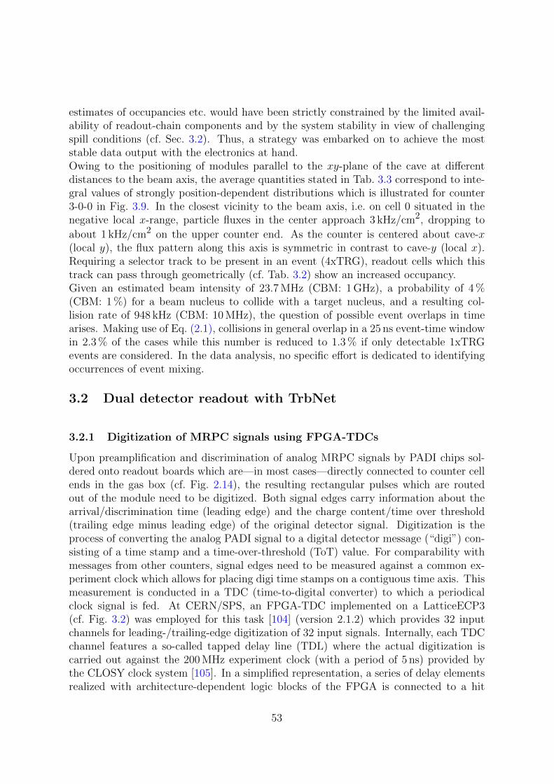
estimates of occupancies etc. would have been strictly constrained by the limited avail-ability of readout-chain components and by the system stability in view of challengingspill conditions (cf. Sec. 3.2). Thus, a strategy was embarked on to achieve the moststable data output with the electronics at hand.Owing to the positioning of modules parallel to the xy-plane of the cave at differentdistances to the beam axis, the average quantities stated in Tab. 3.3 correspond to inte-gral values of strongly position-dependent distributions which is illustrated for counter3-0-0 in Fig. 3.9. In the closest vicinity to the beam axis, i.e. on cell 0 situated in thenegative local x-range, particle fluxes in the center approach 3 kHz/cm2, dropping to

about 1 kHz/cm2 on the upper counter end. As the counter is centered about cave-x(local y), the flux pattern along this axis is symmetric in contrast to cave-y (local x).Requiring a selector track to be present in an event (4xTRG), readout cells which thistrack can pass through geometrically (cf. Tab. 3.2) show an increased occupancy.Given an estimated beam intensity of 23.7 MHz (CBM: 1 GHz), a probability of 4 %(CBM: 1 %) for a beam nucleus to collide with a target nucleus, and a resulting col-lision rate of 948 kHz (CBM: 10 MHz), the question of possible event overlaps in timearises. Making use of Eq. (2.1), collisions in general overlap in a 25 ns event-time windowin 2.3 % of the cases while this number is reduced to 1.3 % if only detectable 1xTRGevents are considered. In the data analysis, no specific effort is dedicated to identifyingoccurrences of event mixing.

3.2 Dual detector readout with TrbNet

3.2.1 Digitization of MRPC signals using FPGA-TDCs

Upon preamplification and discrimination of analog MRPC signals by PADI chips sol-dered onto readout boards which are—in most cases—directly connected to counter cellends in the gas box (cf. Fig. 2.14), the resulting rectangular pulses which are routedout of the module need to be digitized. Both signal edges carry information about thearrival/discrimination time (leading edge) and the charge content/time over threshold(trailing edge minus leading edge) of the original detector signal. Digitization is theprocess of converting the analog PADI signal to a digital detector message (“digi”) con-sisting of a time stamp and a time-over-threshold (ToT) value. For comparability withmessages from other counters, signal edges need to be measured against a common ex-periment clock which allows for placing digi time stamps on a contiguous time axis. Thismeasurement is conducted in a TDC (time-to-digital converter) to which a periodicalclock signal is fed. At CERN/SPS, an FPGA-TDC implemented on a LatticeECP3(cf. Fig. 3.2) was employed for this task [104] (version 2.1.2) which provides 32 inputchannels for leading-/trailing-edge digitization of 32 input signals. Internally, each TDCchannel features a so-called tapped delay line (TDL) where the actual digitization iscarried out against the 200 MHz experiment clock (with a period of 5 ns) provided bythe CLOSY clock system [105]. In a simplified representation, a series of delay elementsrealized with architecture-dependent logic blocks of the FPGA is connected to a hit

53

register of D flip-flops each equipped with a data input D, an edge-sensitive clock inputC, and an output Q. When an input signal propagates through a delay element, thebinary logic level at the D-input of the connected flip-flop changes which repeatedlyoccurs in subsequent delay elements until the state of the entire hit register, i.e. theseries of output states Q reflecting the respective input states D, is latched by the si-multaneous arrival of the next rising edge of the 200 MHz clock signal at all C-inputs.The pattern of logic levels 0 and 1 read from the hit register expresses the arrival timedifference between the input signal and the clock signal at the TDL in terms of delayelements the signal propagated through before the clock signal arrived. By this means, acoarse-time measurement with the 5 ns granularity of the clock period is complementedby a fine-time interpolation with delay elements. As signal delays caused by individualelements of the delay line are not uniform and also depend on operating temperature ofthe FPGA, the fine-time measurement needs to be calibrated (cf. Sec. 3.3). The 11-bitcoarse-time counter implemented in each TDC channel covers a time interval of 10.24µs(called an epoch) and is extended by a single 28-bit epoch counter in the TDC—servingall channels—which is incremented when its own coarse counter overflows. The cali-bration software needs to keep track of overflows in the epoch counter occurring every2748.8 s. Coarse- and (10-bit) fine-time information along with the channel index andthe signal edge type (leading or trailing) form a 4-byte time word which is stored forevery measurement in a 128-word channel ring buffer, together with a 4-byte epoch wordif and only if the epoch counter has been incremented since the previous measurement.In total, 12 bytes of hit data are generated for a signal edge pair not split between twosubsequent epochs. The ring buffer has a capacity to safely store data from about 40input signals, digitized in different TDC epochs, leaving some margin for buffer overflowhandling. To measure leading- and trailing-edge arrival times of the input signal in asingle TDL given a TDC channel dead time of about 20 ns while the hit register is readout and the hit data stored in the ring buffer, the input signal is artificially stretched.For this reason, ToT values measured by the TDC do not directly correspond to thewidth of PADI output signals (cf. Sec. 3.3).

3.2.2 The centrally controlled trigger and readout process

While the FPGA-TDC autonomously digitizes signal-edge arrival times and stores thecorresponding data in ring buffers, it does not automatically push the data towardsthe back end as the self-triggered GET4 chip [81]—the default TDC solution for CBMTOF—would do. Instead, it requires to be embedded in a data-pull architecture whichfetches data from the TDC front end. Such a conventional trigger system based onthe TrbNet protocol [94] (details in [106]) with a central controller sending trigger andreadout requests to and receiving data from front-end nodes was operated at CERN/SPS(cf. Fig. 3.10). The central TrbNet controller, the Central Trigger System (CTS) [107],implemented on the central FPGA of a (master) TRB3 board (cf. Fig. 3.2) communicatesvia optical (off-board) and electrical (on-board) connections with TDC endpoints whichare placed either on peripheral FPGAs of a (master/slave) TRB3 board or on customized

54

RE21 cave

counter site rack corner

CLOSY MBS trigger logic

2 – 5 mFEE

FEE

FEE

FEE

FEE

FEE

FEE

FEE

FEE

FEE

FEE

FEE

hub

CTS

10G

bE s

witc

h

10GbENIC

event builder (PC)

counting house

~50 m

dataslow control

dataslow control

data

data

trigger, data, slow control

trigger, data, slow control

reference time signal

clock signal

trig

ger

sig

nal

trigger, slow control

trigger, slow control

copper cableoptical-fiber cable

hub

Figure 3.10: Sketch of the TrbNet-based data acquisition implemented at CERN/SPS.Upon reception of an external trigger signal by the MBS trigger logic, the Central Trig-ger System (CTS) first sends a reference time signal to the FEE-TDCs—mounted closeto the detectors and synchronized by the clock system CLOSY—which marks the upperend of the trigger window for TDC channel-buffer readout (cf. Fig. 3.11, right plot).Then, via central and peripheral TrbNet hubs, the CTS sends a trigger packet to theTDC endpoints and stays in busy state (ignoring any further external or internal trig-ger input) until it receives a busy-release packet from all endpoints indicating standbyfor another trigger cycle. In a separate readout process, the data stored in the FEEsubsubevent buffers are requested to be sent towards the CTS and—on the first centralFPGA of a TRB3 board which the FEE data packets arrive at—merged into subeventsand bridged from TrbNet to Gigabit Ethernet (GbE). Several GbE data uplinks transmit-ting subevent data are combined into a single 10 Gigabit Ethernet (10GbE) connectionby a dedicated switch. Via optical-fiber cable, the data are transported from the caveto the counting house and the final event is constructed from associated subevents byevent-building software running on the DAQ PC from which slow-control messages canbe sent to all TrbNet nodes via the CTS.

front-end cards in the vicinity of the detectors which were exclusively used as TDCs atCERN/SPS. Slave TRB3 boards without a CTS running on their respective centralFPGA serve as hubs forwarding requests from the CTS and responses by endpointson one of three logical TrbNet channels: a trigger channel to collect and tag front-enddata for readout, a readout channel for data transport, and a slow-control channel forconfiguration—all realized on one physical link. FEE-TDC (front-end electronics) cards

55

are integrated into the DAQ network via peripheral and central hubs on master and slaveTRB3 boards. Round-trip times of packets in this (rather small) star-topology networkat CERN/SPS amount to about 5µs which—ignoring preparation times for event datain the TDC endpoints—imposes a limit of 200 kHz on theoretically achievable triggerrates. Actually, delays originating from network latency in a centrally controlled DAQsystem disqualify its deployment in the CBM experiment from a technical point of view.A trigger decision by the CTS is taken either periodically with respect to an internalpulser signal recurring at a fixed frequency or depending on coincidences in time betweentrigger signals obtained from individual counters responding to physical events. Hence,a dual readout strategy is pursued. The periodical readout of front-end buffers in theformer case could be regarded as a mockup of a self-triggered data acquisition in anintrinsically triggered framework. Physics triggers result from coincident firing of anydiamond channel (the logical OR of signals from all channels) and of any group of fourneighboring MRPC cells on both ends (which are read out by the same two four-channelPADI chips). In total, 7 trigger signals derived from AND circuits between 7 MRPCsin the setup (including three counters in the lower branch) and the rear plane 5-1-0 ofthe double-diamond detector (the front plane, 5-0-0, is not considered) are generated byan external VULOM trigger logic and injected into the trigger logic of the CTS. Upondetecting a rising edge in a trigger input module—either from a periodical pulser or froman external trigger signal—the associated trigger channel is activated and a new TrbNettrigger process is started (cf. Fig. 3.10) if the previous one has been completed.First, the CTS sends a differential reference time signal to all TDC endpoints via directelectrical connections outside TrbNet of varying lengths depending on the position of therespective TDC card in the setup. Splitting is provided by dedicated trigger distributionboards. The rising edge of this signal is measured by a reference channel which everyTDC features in addition to its 32 input channels. Concerning synchronization of clock(coarse) counters among different TDCs, a system-wide counter reset can be issued onDAQ startup upon arrival of the first reference time signal at each TDC to correct fortime offsets, apart from shifts attributed to different trigger cable lengths. The sameprocedure can be performed in calibration software with digitized reference time stamps(cf. Sec. 3.3). In the TrbNet trigger process, the arrival of the reference signal starts thereadout of channel ring buffers into the subsubevent buffer of the TDC endpoint, a 4096-word (16 kiB) FIFO with sufficient storage capacity for data from 32 completely filled128-word channel ring buffers. While in self-triggered mockup operation all data residingin the ring buffers are read out, only a small fraction of data with time stamps fallinginto a trigger window (cf. Fig. 3.11, right plot) defined with respect to the reference timestamp is transferred to the subsubevent buffer if the system is driven by physics triggers.As the generation of trigger signals from combinations of detectors and the broadcastof the reference time signal by the CTS upon a positive trigger evaluation are delayedregarding the arrival time of counter signals at the TDC, the reference coarse-time stamp(including epoch information) is compared backwards in time against the coarse-timestamps of time-sorted channel data in the ring buffers. Channel signals which weredigitized prior to an adjustable time difference to the reference signal, i.e. which do notfit into the trigger-window range, are discarded.

56

0 50 100

event window [ns]

0

0.05

0.1

0.15

0.2610×

dig

i eve

nts

[]

500− 400− 300− 200− 100− 0 100

time to trigger [ns]

0

50

100

150

200

310×

TD

C h

its /

ns []

Figure 3.11: Exemplary event building in software from (calibrated) digital detectormessages distributed in time in ascending order if TrbNet is triggered periodically, i.e.not linked to any correlation of physical signals in a combination of trigger detectors(left plot). With an increasing temporal size of the event window always starting with adiamond digi, an “event step” appears when—depending on the synchronization betweenTDCs—digi pairs from additional detectors required to be present fall into the window aswell (here: 3-0-0 and 4-0-0). If the readout system is driven by (a coincidence matrix of)physics triggers instead (right plot), all detector signals digitized by the TDC (raw TDChits) up to an adjustable point in time (here: −400 ns) prior to the arrival time of thetrigger signal at the TDC (which is delayed due to trigger-logic latency) are consideredto belong to the same physical event. Normally, no further event building in software isnecessary in this case. The double-peak structure indicates a superposition of differenttrigger conditions.

In the meantime, a TrbNet trigger packet has been prepared by the CTS and sent overthe DAQ network including an event tag which the data from the ongoing (or alreadycompleted) transfer between channel ring buffers and subsubevent buffer in the TDCendpoint is marked with. When this data transfer is finished and the tagged subsubeventdata are available for readout from the buffer, the endpoint replies to the CTS triggerpacket with a busy-release packet, signaling readiness for reception of a subsequenttrigger request. The CTS, in turn, waits for the arrival of busy-release packets fromall TDC endpoints in the system before pushing a token with the current event taginto the readout queue and switching from busy to idle state, ready to process triggerinput signals which are ignored while the CTS is busy. Readout operations on thecorresponding channel of TrbNet are executed by the CTS asynchronously to triggerprocesses although they depend on the availability of a token in the readout queue.TrbNet does not suspend all trigger requests until the data from a single trigger andreadout process have been extracted from the system as the TDC endpoint buffers can—under normal operating conditions with an active trigger window—store data of manysubsubevents. Even in the unlikely case of all TDC channels (including the referencechannel) firing in an event in physics-triggered mode, the resulting subsubevent of size392 B (32×12 B+1×8 B) is rather small compared to a FIFO capacity of 16 kiB. Whenthe TDC endpoint receives a readout request by the CTS, it sends the corresponding

57

subsubevent data in its buffer via TrbNet towards the central controller. On the firstcentral hub which the TDC data packets arrive at (whether on the CTS FPGA itself oron the central hub of a slave TRB3 board), subsubevent data from all connected TDCdownlinks are combined into a single subevent which is extracted from the ongoingreadout process and filled into a subevent buffer. Data residing in the subevent FIFOare—by further encapsulation—prepared for transmission via Gigabit Ethernet (GbE) tothe PC serving as event builder, i.e. combining subevents received from different TRB3boards and writing the final event data to disk in a list-mode format. At CERN/SPS,the DABC (Data Acquisition Backbone Core) framework [108] (version 2.7.1) was usedfor this purpose.

3.2.3 Bandwidth limitations and event yields

The bottleneck for data transport in the DAQ system are the GbE uplinks towards theevent builder. If several TDC endpoints are connected to a single TRB3 data concen-trator, they need to share the same uplink which transmits 8-bit data words at a rateof 125 MHz (net bit rate: 1 Gbit/s). However, this technical bandwidth cannot be fullyexploited due to idle time introduced by Ethernet frame construction between trans-mission of consecutive frames, limiting the achievable net bit rate to about 100 MB/s(800 Mbit/s) [109]. On links between TrbNet nodes, however, 16-bit data words areexchanged at a rate of 100 MHz (net bit rate: 1.6 Gbit/s), i.e. even a single TDC end-point can saturate the GbE uplink if the channel data load is sufficiently high. Owingto the interdependence of trigger and readout processes in a centrally controlled setup,the most heavily loaded component puts the entire system on hold. In physics-triggeredoperation with a trigger window in place selecting only a small share of TDC channeldata for readout, it is rather unlikely to reach the GbE bandwidth limit.The situation for a self-triggered mockup, though, is different. When the reference timesignal arrives at the TDC endpoints, the readout of all channel data generated fromsignals of heavy-ion collision secondaries on the connected detectors since the previoustrigger is started. Here, depending on collision rates in conjunction with readout-celloccupancy, data uplink capacities of the DAQ system can be exhausted more easily.Applying a periodical trigger frequency which takes into account estimated channel hitrates and limited ring-buffer sizes not to risk buffered data to be overwritten by subse-quent hits due to too large readout intervals does not ensure loss-free data taking alone,if data transmission speed is a limiting factor. Referring, as an illustrative example,to (idealized) Monte Carlo calculations in Sec. 3.1.3, TDC channel hit rates of about50 kHz can be inferred from a theoretical event rate of 515 kHz under 1xTRG conditionswith a single readout cell being occupied in 10 % of these cases on average. Assumingequal hit distances in time of 20µs—placing hits in different TDC epochs—the mini-mum readout frequency for a ring buffer filled with a maximum of 40 hits amounts to1.25 kHz. For the argon test beam, different trigger frequencies of 10 and 20 kHz wereused to keep fill levels of subsubevent buffers at moderate values. Even higher triggerrates might have stressed the event-building software on the DAQ PC beyond processing

58

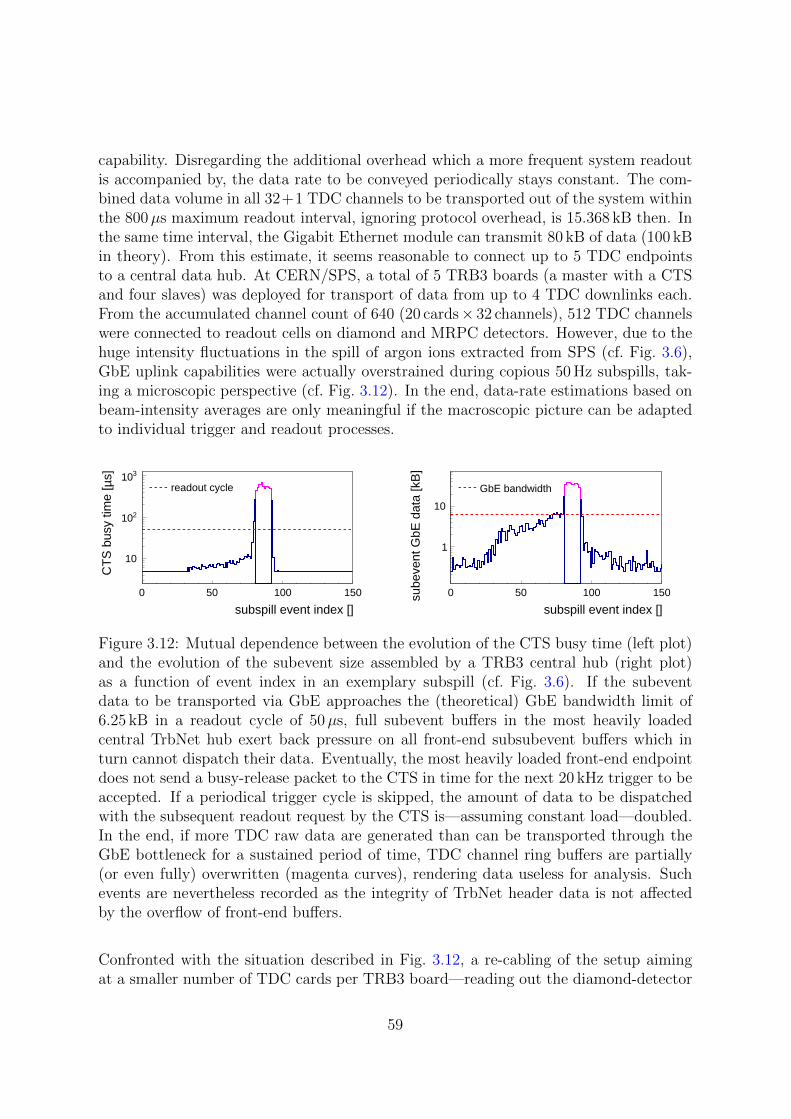
capability. Disregarding the additional overhead which a more frequent system readoutis accompanied by, the data rate to be conveyed periodically stays constant. The com-bined data volume in all 32+1 TDC channels to be transported out of the system withinthe 800µs maximum readout interval, ignoring protocol overhead, is 15.368 kB then. Inthe same time interval, the Gigabit Ethernet module can transmit 80 kB of data (100 kBin theory). From this estimate, it seems reasonable to connect up to 5 TDC endpointsto a central data hub. At CERN/SPS, a total of 5 TRB3 boards (a master with a CTSand four slaves) was deployed for transport of data from up to 4 TDC downlinks each.From the accumulated channel count of 640 (20 cards× 32 channels), 512 TDC channelswere connected to readout cells on diamond and MRPC detectors. However, due to thehuge intensity fluctuations in the spill of argon ions extracted from SPS (cf. Fig. 3.6),GbE uplink capabilities were actually overstrained during copious 50 Hz subspills, tak-ing a microscopic perspective (cf. Fig. 3.12). In the end, data-rate estimations based onbeam-intensity averages are only meaningful if the macroscopic picture can be adaptedto individual trigger and readout processes.

0 50 100 150

subspill event index []

10

210

310s]µ C

TS

bus

y tim

e [ readout cycle

0 50 100 150

subspill event index []

1

10

sub

even

t GbE

dat

a [k

B]

GbE bandwidth

Figure 3.12: Mutual dependence between the evolution of the CTS busy time (left plot)and the evolution of the subevent size assembled by a TRB3 central hub (right plot)as a function of event index in an exemplary subspill (cf. Fig. 3.6). If the subeventdata to be transported via GbE approaches the (theoretical) GbE bandwidth limit of6.25 kB in a readout cycle of 50µs, full subevent buffers in the most heavily loadedcentral TrbNet hub exert back pressure on all front-end subsubevent buffers which inturn cannot dispatch their data. Eventually, the most heavily loaded front-end endpointdoes not send a busy-release packet to the CTS in time for the next 20 kHz trigger to beaccepted. If a periodical trigger cycle is skipped, the amount of data to be dispatchedwith the subsequent readout request by the CTS is—assuming constant load—doubled.In the end, if more TDC raw data are generated than can be transported through theGbE bottleneck for a sustained period of time, TDC channel ring buffers are partially(or even fully) overwritten (magenta curves), rendering data useless for analysis. Suchevents are nevertheless recorded as the integrity of TrbNet header data is not affectedby the overflow of front-end buffers.

Confronted with the situation described in Fig. 3.12, a re-cabling of the setup aimingat a smaller number of TDC cards per TRB3 board—reading out the diamond-detector

59

and the four MRPCs in the upper setup only—would have been a logical step to takefor mitigation of data loss resulting from overwritten channel buffers. Theoretically, theload of 7 TDCs (1 TDC for 16 single-ended cells of diamond detector 5-1-0, 2 TDCs for32 double-ended cells of counter 3-0-0, 2 TDCs for 24 double-ended cells of counter 9-0-0,1 TDC for 16 double-ended cells of counter 7-0-0, and 1 TDC for 16 double-ended cellsof counter 4-0-0) could have been distributed to 5 data hubs to increase the recordedamount of usable event data. Practically, however, such mending efforts were impossi-ble to undertake in the ongoing test beam. On Wednesday evening, March 4, between07:27:03 and 08:09:09 p.m. (total duration: 00:42:06 hours), the self-triggered TrbNetmockup was operated to continuously record collision data from 43 accelerator spills—with interruptions for changing readout frequencies and trying different configurationsfor data transport (sending multiple subevents in a single UDP datagram and usinglarger Ethernet jumbo frames to increase throughput). Following event building fromtime-calibrated detector digis in CbmRoot (cf. Fig. 3.11, left plot), not to be confusedwith the composition of DAQ events from multiple subevent streams by DABC, about11.5 M physical events could be extracted from the recorded mockup data, scanning—insoftware—a 75 ns event window, opened by the time stamp of a 5-1-0 diamond digi,for an additional digi pair on counter 3-0-0 (which geometrically shadows almost theentire rear part of the setup; cf. Tab. 3.2). Complementing the dual readout strat-egy at CERN/SPS, a physics-triggered run was conducted—with interruptions due tomaintenance work at the parallel TRD setup in the cave—under similar experimentalconditions on Thursday morning, March 5, between 00:47:00 and 05:49:36 a.m. (totalduration: 05:02:36 hours), yielding 6.4 M events distributed over 383 spills which wererebuilt in software for a better comparability with mockup data and to dispose of poten-tially multiple diamond hits in the TDC trigger window. Both runs were fully calibratedand analyzed with virtually identical results but only the physics-triggered run is furtherconsidered in this work as it contains—despite a smaller overall event number—morestatistics for the small counter 4-0-0 in the back, owing to the weighted mix of triggercombinations generating the original DAQ event sample, which is needed as a referencecounter for data analysis.Monitoring of conditions and occurrences in the experimental zone took place from asafe distance in a counting house. The system status was shown on various live displaysfor particle fluxes on scintillators (cf. Sec. 3.1.2) and counters, for TDC channel rates, forbasic correlations between counters computed online in CbmRoot, etc. Selected differ-ences between self-triggered mockup and physics-triggered regular operation of TrbNetare depicted in Fig. 3.13, visible on CTS and DABC monitors, respectively, during beamtime.

60

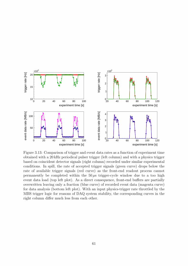
0 20 40 60 80 100

experiment time [s]

10

15

20

310×

trig

ger

rate

[Hz]

20 40 60 80 100 120

experiment time [s]

0

1

2

3

310×

trig

ger

rate

[Hz]

0 20 40 60 80 100

experiment time [s]

50

100

eve

nt d

ata

rate

[MB

/s]

20 40 60 80 100 120

experiment time [s]

0

1

2

3

4

eve

nt d

ata

rate

[MB

/s]

Figure 3.13: Comparison of trigger and event data rates as a function of experiment timeobtained with a 20 kHz periodical pulser trigger (left column) and with a physics triggerbased on coincident detector signals (right column) recorded under similar experimentalconditions. In spill, the rate of accepted trigger signals (green curve) drops below therate of available trigger signals (red curve) as the front-end readout process cannotpermanently be completed within the 50µs trigger-cycle window due to a too highevent data load (top left plot). As a direct consequence, front-end buffers are partiallyoverwritten leaving only a fraction (blue curve) of recorded event data (magenta curve)for data analysis (bottom left plot). With an input physics-trigger rate throttled by theMBS trigger logic for reasons of DAQ system stability, the corresponding curves in theright column differ much less from each other.

61

3.3 Raw-data calibration and hit building

Hit data read out from TDC channels during data acquisition contain coarse- (epochincluded) and fine-time information reflecting subsequent arrival times of both inputsignal edges at the delay line with respect to the experiment clock. In order to convertTDC hit data to a digital detector message (“digi”), the final raw-data format in Cbm-Root, values of coarse- and fine-time counters need to be translated into time stamps.Regarding coarse time, the corresponding counter value is multiplied with the systemclock period of 5 ns and counter overflows are kept track of. The spectrum of occupiedfine-time bins obtained for all hits in a TDC channel reflects the arrival-time differencesbetween input signals and the clock signal which samples the delay line, with a mini-mum of 0 ns attributed to the lower end of the spectrum (lower edge of bin bmin) and amaximum of 5 ns (a clock period) ascribed to the upper end (upper edge of bin bmax).An obvious translation method between fine-time bin i and a distance in time to thenext rising edge of the clock signal is a linear interpolation between bin centers,

ft(i) =τclk

bmax − bmin + 1

(i− (bmin − 1)− 1

2

), (3.5)

τclk referring to the clock period. However, fluctuations in relative frequencies of fine-time bins (cf. Fig. 3.14, left plot) caused by varying lengths of individual delay elements(so-called non-linearities) should be accounted for to utilize the full resolving capacity ofthe TDC [104]. With sufficient statistics available for a TDC channel, an interpolationrespecting relative frequencies nk of N occupied fine-time bins,

ft(i) = τclk

(i∑

k=1

nk −1

2ni

)/N∑k=1

nk, (3.6)

yields better time resolutions between reference channels of TDCs 1–19 and of TDC 0,respectively, the latter of which specifies the common experiment time axis all measuredtime stamps are to be arranged on (cf. Fig. 3.14, middle plot).Concerning the significantly worse time resolution obtained for TDC 13 digitizing cellsignals from the front diamond detector 5-0-0 (not considered hereafter), some addi-tional jitter might have been introduced on the reference time signal by cabling. AsGaussian sigmas of time-difference spectra between measurements of the same signal bytwo different TDCs are plotted, single-TDC resolutions can be derived by dividing thegiven numbers by the square root of two. A time-difference resolution of 20 ps corre-sponds to a single-TDC resolution of 14 ps. If coarse counters across TDCs are not resetsimultaneously on system startup, a time-offset correction with respect to TDC 0 canbe performed based on reference-channel information prior to further calibration steps(cf. Fig. 3.14, right plot). It is more a matter of convenience than of necessity, though,as signal propagation offsets due to routing differences between counter cells to a TDCand between neighboring TDC channels on the same FPGA need to be corrected for ina later iteration anyway. Now, a digi featuring a (continuous) time stamp and a timeover threshold (ToT) can be generated from a leading-/trailing-edge TDC measurement

62

0 200 400

channel fine time [bins]

0

50

100

310×

hits

/ F

T b

in []

0 5 10 15 20

TDC index []

0

10

20

30

40

t) [p

s]∆(σ

ref

cha

nnel

0 5 10 15 20

TDC index []

1

210

410

610

810

1010

1210

t) [5

ns]

∆(µ r

ef c

hann

el

Figure 3.14: Non-linearity of TDC fine-time interpolation by the tapped-delay-line(TDL) method in an exemplary TDC channel (left plot). Gaussian sigmas of time-difference spectra between the reference channel of every TDC in the setup against ref-erence TDC 0 (middle plot). The black circles are obtained with a linear interpolationbetween all occupied fine-time bins (cf. Eq. (3.5)) while the blue squares result from anestimation of actual fine-time bin widths based on relative bin occupancy (cf. Eq. (3.6)).Gaussian mean shifts between reference-channel coarse counters result from latency inthe DAQ network if a global coarse-counter reset is issued via TrbNet slow control and—concerning TDCs 8–11—from individual power cycling not followed by a common reset(right plot).

and—with an addressing scheme extending the three-digit counter identifier by a cellindex and a cell-side index (0 for negative local y, 1 for positive)—be traced back to itsgeometric origin in the test-beam setup.Position and time of a particle hit on the counter surface are reconstructed from the in-dex of the cell on which the signal was induced (local x; cf. Eq. (3.1)), from the differencebetween time stamps on opposing cell ends (local y; cf. Eq. (3.3)), and from the averageof time stamps minus half the signal propagation time along the full cell of length s,

t = 1/2(t− + t+

)− 1/2 s/vsignal. (3.7)

Measured time stamps t− and t+ depend on position y0 and time t0 of the induction“spot” on the cell and on the aforementioned signal propagation times to the delayline in the TDC which vary from cell to cell, labeled with c− and c+ in the following.Actually, the latter quantities are functions of the signal amplitude, i.e. the time overthreshold, as larger signals are discriminated and digitized earlier in time than smallersignals which is discussed later in this section. Ignoring uncertainties of the inductionprocess and measurement resolutions, digitized signals on opposing cell ends would betime-stamped according to

t− = t0 + (s/2 + y0) /vsignal + c− and (3.8)

t+ = t0 + (s/2− y0) /vsignal + c+,

with unknowns c− and c+ to be determined from residuals between reconstructed cellhits and a reference. Inserting these expressions into Eqs. (3.3) and (3.7), residuals in y

63

and in t are obtained presuming ideal knowledge of hit position and time on the cell,

ry := yhit − y0 = 1/2(c− − c+

)vsignal and (3.9)

rt := thit − t0 = 1/2(c− + c+

).

Outside of a Monte Carlo simulation, y0 and t0 are not known. To determine routingoffsets c− and c+ for experimental data, these reference values need to be extracted fromthe data itself, in addition to the signal velocity vsignal. Starting from the mere time-difference spectrum dt between signals on opposing cell ends due to a lack of knowledgeon vsignal,

dt := 1/2(t− − t+

), (3.10)

offsets can be constrained by requiring the dt-spectrum to be centered about zero whichdoes not necessarily imply shifting the mean value of dt to the point of origin as thespectrum—depending on the irradiation profile on the cell—might not be axially sym-metric. The deviation of the measured average dt from the mean value of a centereddt-spectrum,

〈dt〉hit − 〈dt〉central = 1/2(〈c−〉 − 〈c+〉

), (3.11)

directly corresponds to half the time difference between mean values of c− and c+, anglebrackets here denoting integration over ToT-dependencies of the two propagation-timeoffsets. The second boundary condition required for an unambiguous determination ofthese quantities is given by an alignment of the reconstructed hit time on the cell to areference time measured within the same event,

〈thit − t0〉 = 1/2(〈c−〉+ 〈c+〉

). (3.12)

As an arrangement of hit times on the experiment time axis according to physical time-of-flight information between different stations—which could be obtained from a MonteCarlo simulation (cf. Tab. 3.2 for the shortest TOF values between target and counters)—is not needed for the χ2-analysis of residuals conducted later in this work (cf. Chap. 5), noextrapolation of the reference time towards the physical hit time on the cell to calibrateis performed. In the first calibration instance, the reference time is provided by diamonddetector 5-1-0 in each event. As a result, calibrated hits on all cells in the setup occur—on average—simultaneous to the time stamp of the diamond measurement. CombiningEqs. (3.11) and (3.12) allows for calculating mean propagation-time offsets at both cellends according to

〈c−〉 = 〈thit − t0〉+ 〈dt〉hit − 〈dt〉central and (3.13)

〈c+〉 = 〈thit − t0〉 − 〈dt〉hit + 〈dt〉central.

Concerning reconstruction of hit position and time on diamond cells which are read outon a single end only, a fixed position along the cell of y0 can be freely assigned (zero inthis case) which enters the calculation of hit times from a single digi time stamp,

t = t− − (1/2 s+ y0)/vsignal. (3.14)

64

Also, this leaves a single offset parameter c− to be determined for temporal alignment ofdiamond cells against an MRPC reference cell. Due to the position spread of beam-ionhits along the 1.8 cm long diamond cells which is not accounted for by a single-endedreadout, some additional jitter is introduced to the time residual between the diamondand counters in the setup. Since these residuals are considered for calibration only andnot for performance evaluation during analysis (done exclusively between MRPCs), thiseffect is not of any relevance.

0 5 10 15

Dia cell []

0

20

40

60

cel

l [ns

]t

MR

PC

- D

ia r

1

10

210

310

0 5 10 15 20

MRPC cell []

10−

0

10

20 c

ell [

ns]

t M

RP

C -

Dia

r

1

10

210

310

0 5 10 15 20

MRPC cell []

4−

2−

0

2

4

cel

l [ns

]t

MR

PC

d

1

10

210

310

0 5 10 15

Dia cell []

4−

2−

0

2

4

cel

l [ns

]t

MR

PC

- D

ia r

1

10

210

310

0 5 10 15 20

MRPC cell []

4−

2−

0

2

4

cel

l [ns

]t

MR

PC

- D

ia r

1

10

210

310

0 5 10 15 20

MRPC cell []

1−

0

1 c

ell [

ns]

t M

RP

C d

1

10

210

310

Figure 3.15: Cell-based time and position offsets after TDC calibration (upper row)and after corrections (lower row). Cell time residuals of diamond detector 5-1-0 againstan MRPC reference cell of counter 3-0-0 (left column). Cell time residuals of counter9-0-0 against a calibrated diamond reference cell (middle column). Top/bottom time-difference spectra of cells on counter 9-0-0 (right column). Profile lines in the lower rowindicate cell averages.

The first step taken to calibrate digi time stamps for offsets in time and position isindependent from a geometrical matching in xyz between cell hits on different countersas individual MRPC cells are compared against diamond cells and not against each other.A hit on the diamond prior to a collision event in the target imposes no directional biason particle trajectories in the setup. At this calibration level, only cell hits reconstructedfrom the earliest top/bottom digi pair on a counter cell in the respective event (a singledigi in the diamond case) are considered. Noisy or dead cells are excluded from thisprocedure (cf. Tab. 3.4). For cell alignment on the diamond detector, residuals betweendiamond cells and a reference cell on counter 3-0-0 (cf. Fig. 3.15), generated from theentire event sample, are shifted to zero mean. Apart from further smoothing betweenneighboring diamond cells in the course of calibration, preserving the overall average,

65

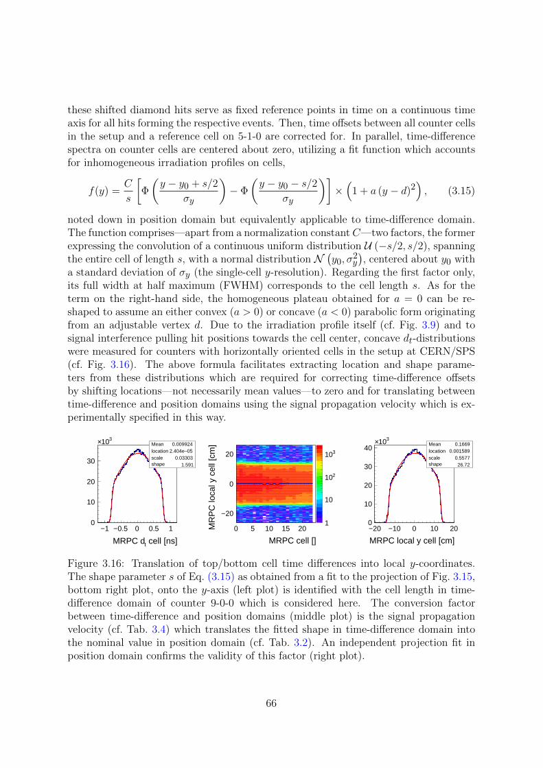
these shifted diamond hits serve as fixed reference points in time on a continuous timeaxis for all hits forming the respective events. Then, time offsets between all counter cellsin the setup and a reference cell on 5-1-0 are corrected for. In parallel, time-differencespectra on counter cells are centered about zero, utilizing a fit function which accountsfor inhomogeneous irradiation profiles on cells,

f(y) =C

s

[Φ

(y − y0 + s/2

σy

)− Φ

(y − y0 − s/2

σy

)]×(

1 + a (y − d)2), (3.15)

noted down in position domain but equivalently applicable to time-difference domain.The function comprises—apart from a normalization constant C—two factors, the formerexpressing the convolution of a continuous uniform distribution U (−s/2, s/2), spanningthe entire cell of length s, with a normal distribution N

(y0, σ

2y

), centered about y0 with

a standard deviation of σy (the single-cell y-resolution). Regarding the first factor only,its full width at half maximum (FWHM) corresponds to the cell length s. As for theterm on the right-hand side, the homogeneous plateau obtained for a = 0 can be re-shaped to assume an either convex (a > 0) or concave (a < 0) parabolic form originatingfrom an adjustable vertex d. Due to the irradiation profile itself (cf. Fig. 3.9) and tosignal interference pulling hit positions towards the cell center, concave dt-distributionswere measured for counters with horizontally oriented cells in the setup at CERN/SPS(cf. Fig. 3.16). The above formula facilitates extracting location and shape parame-ters from these distributions which are required for correcting time-difference offsetsby shifting locations—not necessarily mean values—to zero and for translating betweentime-difference and position domains using the signal propagation velocity which is ex-perimentally specified in this way.

Mean 0.009924location 05− 2.404escale 0.03303shape 1.591

1− 0.5− 0 0.5 1

cell [ns]t MRPC d

0

10

20

30

310× Mean 0.009924location 05− 2.404escale 0.03303shape 1.591

0 5 10 15 20

MRPC cell []

20−

0

20

MR

PC

loca

l y c

ell [

cm]

1

10

210

310

Mean 0.1669location 0.001589scale 0.5577shape 26.72

20− 10− 0 10 20

MRPC local y cell [cm]

0

10

20

30

40310× Mean 0.1669

location 0.001589scale 0.5577shape 26.72

Figure 3.16: Translation of top/bottom cell time differences into local y-coordinates.The shape parameter s of Eq. (3.15) as obtained from a fit to the projection of Fig. 3.15,bottom right plot, onto the y-axis (left plot) is identified with the cell length in time-difference domain of counter 9-0-0 which is considered here. The conversion factorbetween time-difference and position domains (middle plot) is the signal propagationvelocity (cf. Tab. 3.4) which translates the fitted shape in time-difference domain intothe nominal value in position domain (cf. Tab. 3.2). An independent projection fit inposition domain confirms the validity of this factor (right plot).

66

Table 3.4: Counter cells excluded from calibration and clustering and fitted signal prop-agation velocities of calibrated counters (exception: a default value of 18 cm/ns is usedfor the single-ended diamond cells).

counter 5-1-0 3-0-0 9-0-0 7-0-0 4-0-0

dead/disabled cells / 0, 31 23 0, 15 0, 9

signal propagation velocity [cm/ns] 18.0 16.7 16.8 16.0 14.4

The impact of signal induction in the readout plane by a traversing charged particlewhich triggers an avalanche in an MRPC gas gap is not limited to a single cell. Con-sequently, correlations arise between reconstructed hits on adjacent cells, both in timeand in position. These correlations jointly constitute the response of the counter to theparticle crossing its active volume and should be treated as a whole in further calibrationsteps and in data analysis. In Fig. 3.17, this behavior is shown for time residuals andtime differences on neighboring cells, prior to and following upon the initial round ofoffset corrections between cells. On the ordinates, the relations

∆dt := dmt − dnt = 1/2(t−m − t+m

)− 1/2

(t−n − t+n

)and (3.16)

∆rt := rmt − rnt = 1/2(t−m + t+m

)− 1/2

(t−n + t+n

)are plotted to quantify correlations among cells m and n, the latter being located closerto a reference cell on the counter surface which is used as a bidirectional starting point.Fitting distribution peaks with Gaussian functions yields a width for ∆dt which is lessthan half the width obtained for ∆rt although statistical errors on both expressionsare identical according to Eq. (3.16) and can be reduced to the combined electronicsresolution of discrimination and digitization processes in a single readout channel. Thedeviation is caused by the aforementioned dependence of measurement quality on sig-nal amplitude, an effect which cancels out if time stamps from opposing ends of thesame cell are subtracted from each other as is the case for ∆dt but not for ∆rt. Sig-nals induced on multiple readout cells by the same avalanche vary in amplitude dueto increasing distances to the response center, i.e. contributions from cells m and n to∆rt do not neutralize each other in this respect. Criteria for building response clustersfrom individual cell hits should take this initial situation into account. Approximatelyoriented towards 5-sigma intervals of correlation widths obtained for different countersin the setup, distances among hits on adjacent cells are required not to exceed 0.5 ns inresidual time and 0.25 ns in time difference (which translates into a position differenceof 4.5 cm using a default signal velocity of 18 cm/ns). These limits are generally appliedto clustering of cell hits on all counters.A response cluster represents multiple measurements of a single physical interaction be-tween a primary particle and the detection medium. Individual values in this ensembleare obtained with different accuracy, though, as the jitter on leading-edge discriminationis larger, on average, for smaller signals which are induced on the boundary cells of amulti-cell cluster than for bigger signals which are observed on central cells of the cluster.

67

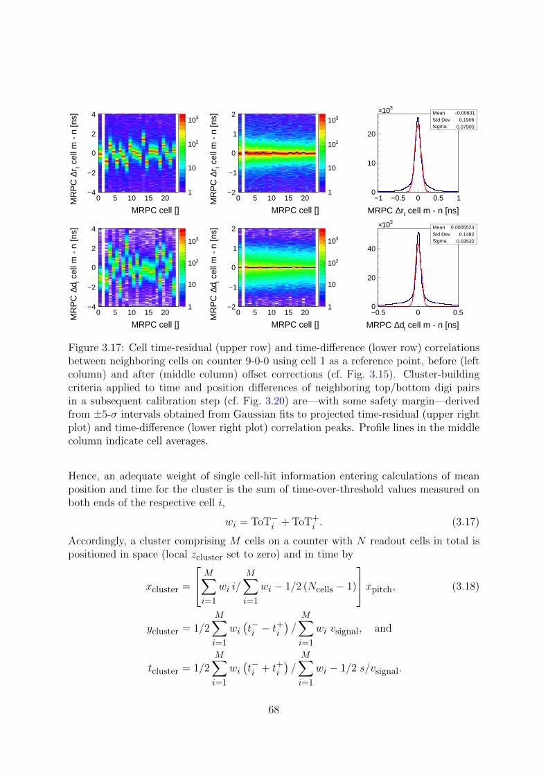
0 5 10 15 20

MRPC cell []

4−

2−

0

2

4

cel

l m -

n [n

s]tr∆

MR

PC

1

10

210

310

0 5 10 15 20

MRPC cell []

2−

1−

0

1

2

cel

l m -

n [n

s]tr∆

MR

PC

1

10

210

310Mean 0.00631− Std Dev 0.1906Sigma 0.07903

1− 0.5− 0 0.5 1

cell m - n [ns]tr∆ MRPC

0

10

20

310× Mean 0.00631− Std Dev 0.1906Sigma 0.07903

0 5 10 15 20

MRPC cell []

4−

2−

0

2

4

cel

l m -

n [n

s]td∆

MR

PC

1

10

210

310

0 5 10 15 20

MRPC cell []

2−

1−

0

1

2

cel

l m -

n [n

s]td∆

MR

PC

1

10

210

310

Mean 0.0005524Std Dev 0.1482Sigma 0.03532

0.5− 0 0.5

cell m - n [ns]td∆ MRPC

0

20

40

310× Mean 0.0005524Std Dev 0.1482Sigma 0.03532

Figure 3.17: Cell time-residual (upper row) and time-difference (lower row) correlationsbetween neighboring cells on counter 9-0-0 using cell 1 as a reference point, before (leftcolumn) and after (middle column) offset corrections (cf. Fig. 3.15). Cluster-buildingcriteria applied to time and position differences of neighboring top/bottom digi pairsin a subsequent calibration step (cf. Fig. 3.20) are—with some safety margin—derivedfrom ±5-σ intervals obtained from Gaussian fits to projected time-residual (upper rightplot) and time-difference (lower right plot) correlation peaks. Profile lines in the middlecolumn indicate cell averages.

Hence, an adequate weight of single cell-hit information entering calculations of meanposition and time for the cluster is the sum of time-over-threshold values measured onboth ends of the respective cell i,

wi = ToT−i + ToT+i . (3.17)

Accordingly, a cluster comprising M cells on a counter with N readout cells in total ispositioned in space (local zcluster set to zero) and in time by

xcluster =

M∑i=1

wi i/M∑i=1

wi − 1/2 (Ncells − 1)

xpitch, (3.18)

ycluster = 1/2M∑i=1

wi(t−i − t

+i

)/M∑i=1

wi vsignal, and

tcluster = 1/2M∑i=1

wi(t−i + t+i

)/M∑i=1

wi − 1/2 s/vsignal.

68

Weighting contributions to the cluster with the respective ToT sum requires ToT spectrameasured on all cell ends of the counter to be comparable, both in mean and in width.For two main reasons, this condition is not met prior to a dedicated alignment of thesespectra: On the one hand, amplification gains of PADI channels in the setup are notuniform yielding different output amplitudes, i.e. varying ToT values, for the same inputsignal. On the other hand, as pointed out in Sec. 3.2, TDC input signals are stretchedto digitize arrival times of both signal edges in a single delay line. This stretchingoffset added to the ToT varies slightly between TDC channels. To compute clustercoordinates, it is not necessary to disentangle PADI and TDC contributions to the shapeof a ToT spectrum (in order to arrive at physical ToT values). Instead, ToT spectra areharmonized by linear transformations aiming at a common mean and standard deviationin arbitrary units,

f (ToT) = mToT + b, (3.19)

utilizing general rules for the expectation value and the variance of a linearly transformedrandom variable X,

E [mX + b] = mE [X] + b and Var (mX + b) = m2 Var (X) . (3.20)

ToT calibration is illustrated in Fig. 3.18. The readout cell with the highest ToT-weightcontributing to the cluster—upon harmonization of ToT spectra—is considered the maincluster cell. Measured cluster sizes vary as a function of main cell across the countersurface for reasons of symmetry (cf. Fig. 3.19). Induction occurring on the central cells ofthe readout plane can affect adjacent cells in two directions while an avalanche triggeredabove a peripheral cell can geometrically only have some further impact towards thecounter center. The mean cluster size measured for a counter depends both on design,in particular on the granularity of its readout cells, and on operating conditions likeelectric field strength in the gas gaps and discrimination threshold. With some selectionbias on counter surfaces due to the mix of hardware-trigger conditions used for datataking, the following mean cluster sizes are obtained for the five counters under consid-eration: 1.00 on 5-1-0 (diamond), 1.59 on 3-0-0, 1.49 on 9-0-0, 1.09 on 7-0-0, and 1.23on 4-0-0, with statistical errors on the mean of the order of 10−4.Upon combining correlated cell hits to clusters by an algorithm which is visualized inFig. 3.20, an iterative calibration procedure eliminates remaining residual offsets betweenclusters and the dependence of time measurements on the signal amplitude (sketchedibid.). Compensation values for average shifts in cluster position and time are attributedto the main cell of the respective cluster and added to c− and c+ for this cell. While po-sition corrections aiming at homogeneously centered y-distributions across the countersurface are performed internally, time residuals to be shifted to zero mean are formedbetween clusters on a counter to calibrate and—alternately—the earliest clusters in anevent on either the diamond detector 5-1-0 (providing a stable overall time reference) orone of two calibration selector counters in the setup, a task assigned to counters 3-0-0and 9-0-0 here. Thus, all counters in the setup are repeatedly calibrated against eachother.When convergence of corrections on cluster residual means is achieved after a few iter-ations, the time-walk effect, i.e. the dependence of the average time residual between

69

0 10 20 30 40

MRPC cell side []

30

40

50

60

70

orig

inal

ToT

[ns]

1

10

210

310

410

Mean y 35.98Std Dev y 2.665

0 10 20 30 40

MRPC cell side []

0

2

4

6

8

10

sca

led

ToT

[a.u

.]

1

10

210

310

410

510Mean y 2Std Dev y 0.5

Mean 35.34Std Dev 2.235

30 40 50 60 70

original ToT cell 11-0 [ns]

1

10

210

310

410

Mean 35.34Std Dev 2.235

Mean 2Std Dev 0.4999

0 2 4 6 8 10

scaled ToT cell 11-0 [a.u.]

1

10

210

310

410

510Mean 2Std Dev 0.4999

Figure 3.18: Original time-over-threshold spectra from each cell side (2*index + 0/1for bottom/top) of counter 9-0-0 as measured by the connected TDC channels whichinternally stretch input signals to detect both leading and trailing edge in a single delayline (upper left plot). Final ToT spectra from each cell side after individually scalingevery spectrum to a common mean of 2 (cf. profile line) and a common standard deviationof 0.5 (upper right plot). Respective projections of bottom-edge ToT spectra of cell 11are shown in the lower row.

clusters on the time over threshold of cell digis, can be mitigated. For this purpose,average deviations of cluster time residuals from the integrated residual mean in typ-ically 0.1 or 0.2 (a.u.) wide scaled-ToT bin slices (with a sufficient number of entries)are calculated individually for each cell end contributing to a cluster on the diamondor on an MRPC, compared against a selector cluster which matches in position. Inthe subsequent iteration, these ToT-dependent deviations are subtracted from digi timestamps, linearly interpolating correction values between ToT bin centers. To increasethe efficiency of time-walk corrections, each round is preceded by a compensation of theparticle velocity spread which is inherent to the time residual between clusters due to thevelocity spectrum of collision secondaries in an event. Corresponding correction valuesagainst the time difference between earliest clusters on the diamond and the active selec-tor counter are not applied permanently to reconstructed cluster time stamps but servethe sole purpose of preparing residuals for the following evaluation of time walk. Be-tween consecutive iterations of velocity and time-walk corrections (depicted in Fig. 3.21),cluster residual means in time and position are repeatedly realigned to compensate forpossible minor shifts introduced by the former procedure. Finally, a calibrated array ofclustered cell hits in each event is available for data analysis (cf. Chap. 5).

70

0 5 10 15 20

cluster main cell []

5

10

15 c

lust

er s

ize

[cel

ls]

1

10

210

310

410

510

Mean y 1.488Std Dev y 0.7661

Mean 1.485Std Dev 0.7722

5 10 15

cluster size cell 11 [cells]

1

10

210

310

410

510

Mean 1.485Std Dev 0.7722

Figure 3.19: Cluster-size distribution of counter 9-0-0 as a function of the main clustercell by ToT-weighting of contributing cells (left plot). Individual cluster-size distributionwith central cell 11 as main cell (right plot).

cell index 7 … 0

local y

0 1 2 3 4 5

time [ns]

0

1

2

3

sig

nal a

mpl

itude

[a.u

.]

discriminationthreshold

Figure 3.20: Illustration of the cluster-building criteria for time and position correlationsbetween neighboring readout cells (left sketch). Scanning the counter surface for hits onneighboring cells starting from cell 0, the two hits marked in black on cells 1 and 2 meetboth criteria while the adjacent hit on cell 3 marked in blue is too far off in position, atleast, to belong to the black cluster, hence starting a new (blue) cluster. With the hiton cell 5 found to be correlated with the hit on cell 3, the blue cluster spans cell 4 whichis declared dead. The hit marked in yellow on cell 6 could position-wise be integratedinto the blue cluster but is not compatible in time with the average of the hits marked inblue, leaving it isolated. Illustration of the time-walk effect, an interplay between signalamplitude and discrimination threshold (right plot). Amplified MRPC signals withidentical rise times but different amplitudes, i.e. charge content (demonstrated by a set ofLandau functions with identical location and scale parameters but varying coefficients),cross the discrimination threshold at different points in time, larger signals earlier thansmaller signals. As the ToT measurement (time difference between threshold crossingpoints of both signal edges) is directly linked to the signal amplitude, this systematictype of timing jitter can be corrected for.

71

5− 0 5

cluster [ns]t Dia - Sel r

0.5−

0

0.5

clu

ster

[ns]

t M

RP

C -

Sel

r

1

10

210

310

410

Mean y 0.04663− Std Dev y 0.1262

0 2 4 6 8 10

MRPC cell ToT [a.u.]

0.5−

0

0.5

clu

ster

[ns]

t M

RP

C -

Sel

r

1

10

210

310

410

Mean y 0.01156− Std Dev y 0.1046

10− 5− 0 5 10

cluster [cm]x MRPC - Sel r

10−

5−

0

5

10

clu

ster

[cm

]y

MR

PC

- S

el r

310

410

5− 0 5

cluster [ns]t Dia - Sel r

0.5−

0

0.5

clu

ster

[ns]

t M

RP

C -

Sel

r

1

10

210

310

410Mean y 0.01029− Std Dev y 0.1085

0 2 4 6 8 10

MRPC cell ToT [a.u.]

0.5−

0

0.5

clu

ster

[ns]

t M

RP

C -

Sel

r

1

10

210

310

410

Mean y 0.0164Std Dev y 0.09791

Figure 3.21: Dependence and its correction of the time residual between a cluster on9-0-0 and the earliest cluster in an event on calibration selector (Sel) counter 3-0-0 onthe time residual between the earliest clusters, respectively, on the diamond detector andon counter 3-0-0 (left column, upper and lower plot). The diagonal trend in the nega-tive abscissa range towards the point of origin reflects increasing velocities of particleswhich propagate from the collision zone to both MRPCs. A significant number of ran-dom assignments under the given experimental conditions constitutes a horizontal bandwhich reduces the effectiveness of an alignment based on bin averages. This (transient)velocity/time-of-flight correction always precedes a subsequent time-walk correction touncover the latter effect on the ordinate residual between MRPCs. As residuals onordinate and abscissa are directly correlated by Sel cluster times entering into bothquantities, the correction is not passed on to analysis. Average time-walk dependenceand its correction (if enough statistics are available in a bin slice) on the average ToT of9-0-0 cells constituting the cluster (middle column, upper and lower plot). Correctionhistograms are filled if a basic matching condition in space (rxy < 2 cm) is met betweenclusters on the counter and on the selector (upper right plot).

72

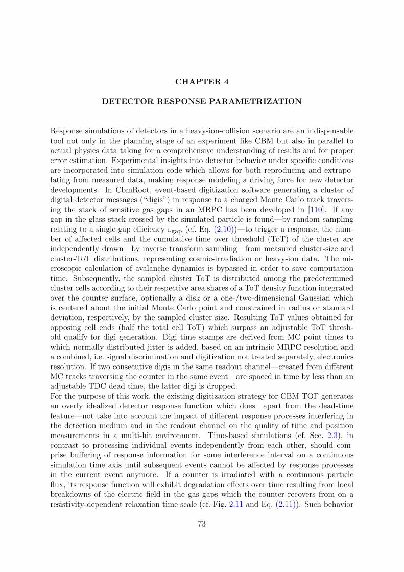
CHAPTER 4

DETECTOR RESPONSE PARAMETRIZATION

Response simulations of detectors in a heavy-ion-collision scenario are an indispensabletool not only in the planning stage of an experiment like CBM but also in parallel toactual physics data taking for a comprehensive understanding of results and for propererror estimation. Experimental insights into detector behavior under specific conditionsare incorporated into simulation code which allows for both reproducing and extrapo-lating from measured data, making response modeling a driving force for new detectordevelopments. In CbmRoot, event-based digitization software generating a cluster ofdigital detector messages (“digis”) in response to a charged Monte Carlo track travers-ing the stack of sensitive gas gaps in an MRPC has been developed in [110]. If anygap in the glass stack crossed by the simulated particle is found—by random samplingrelating to a single-gap efficiency εgap (cf. Eq. (2.10))—to trigger a response, the num-ber of affected cells and the cumulative time over threshold (ToT) of the cluster areindependently drawn—by inverse transform sampling—from measured cluster-size andcluster-ToT distributions, representing cosmic-irradiation or heavy-ion data. The mi-croscopic calculation of avalanche dynamics is bypassed in order to save computationtime. Subsequently, the sampled cluster ToT is distributed among the predeterminedcluster cells according to their respective area shares of a ToT density function integratedover the counter surface, optionally a disk or a one-/two-dimensional Gaussian whichis centered about the initial Monte Carlo point and constrained in radius or standarddeviation, respectively, by the sampled cluster size. Resulting ToT values obtained foropposing cell ends (half the total cell ToT) which surpass an adjustable ToT thresh-old qualify for digi generation. Digi time stamps are derived from MC point times towhich normally distributed jitter is added, based on an intrinsic MRPC resolution anda combined, i.e. signal discrimination and digitization not treated separately, electronicsresolution. If two consecutive digis in the same readout channel—created from differentMC tracks traversing the counter in the same event—are spaced in time by less than anadjustable TDC dead time, the latter digi is dropped.For the purpose of this work, the existing digitization strategy for CBM TOF generatesan overly idealized detector response function which does—apart from the dead-timefeature—not take into account the impact of different response processes interfering inthe detection medium and in the readout channel on the quality of time and positionmeasurements in a multi-hit environment. Time-based simulations (cf. Sec. 2.3), incontrast to processing individual events independently from each other, should com-prise buffering of response information for some interference interval on a continuoussimulation time axis until subsequent events cannot be affected by response processesin the current event anymore. If a counter is irradiated with a continuous particleflux, its response function will exhibit degradation effects over time resulting from localbreakdowns of the electric field in the gas gaps which the counter recovers from on aresistivity-dependent relaxation time scale (cf. Fig. 2.11 and Eq. (2.11)). Such behavior

73

can be observed as a function of event time in an accelerator spill with an event-based,i.e. conventionally hardware-triggered, data acquisition system (cf. Chap. 5) but not bedescribed with event-based simulations in the above sense. Response observables andtheir respective deterioration with irradiation time are, in addition, mutually dependentwhich is not considered in the existing digitization code that splits the response calcu-lation into a series of partially independent sampling processes. A geometrical ten-cellcluster created upon identification of an efficient gap, for instance, should not receivea cluster ToT drawn from the same spectrum which is accessible also to a two-cellcluster, and possibly be reduced to an effective six-cell cluster by ToT discrimination.Instead, the distribution of charge induced on individual cells in the readout plane andthe discrimination of corresponding signals picked up at cell ends with a given thresholddetermine both efficiency and cluster size. Thus, together with a demand for rate-effectand interference handling, there was a need for a more holistic digitization approach.In this chapter, a new digitization algorithm for time-based MRPC response simulationsis described which derives subsequent response observables from an initial sampling oftotal induced charge in the readout plane using a parametrized, i.e. not experimentallydetermined spectrum. Further parametrizations of functions for the distribution of in-duced charge onto individual readout cells and, in particular, for (amplified) signalscontaining half of the respective cell charge facilitate introducing amplitude-dependentdiscrimination jitter and time-residual means (walk) into the code. As a consequence,downscaling the original induced charge spectrum which results in—on average—smallersignal amplitudes directly impacts the response. Model parameters are constrained bya set of measured response observables. The modeling process, features, and limitationsof the new approach are outlined in Sec. 4.1. An extension of the static response casetowards a dynamic irradiation scenario by a particle memory which causes a scalingof the induced charge spectrum depending on the impact of previous particles hittingthe counter on the current one is presented in Sec. 4.2 and used to mimic the physicalbreakdown and recovery of the electric field in the gaps. Lastly, the time-based han-dling of signal interference in the readout channels in CbmRoot is sketched in Sec. 4.3,followed by discussions on reducing execution times of the digitization code via multi-threading/parallelization and on its applicability for test-beam simulations.

4.1 Modeling assumptions and procedure

4.1.1 Signal generation and calibration of simulated data

The parametrization of the MRPC response function developed in this work is notthe result of a strict theoretical derivation—as given in [74], for instance—from firstprinciples of molecular ionization in the gas gaps, followed by avalanche formation ofaccelerated free electrons in the applied electric field and a simultaneous induction ofsignals by avalanche charges moving towards readout cells. To save computation time,microscopic processes are subsumed under a series of functions aiming at describingcomplex response dynamics with a concatenation of static impressions which allows for

74

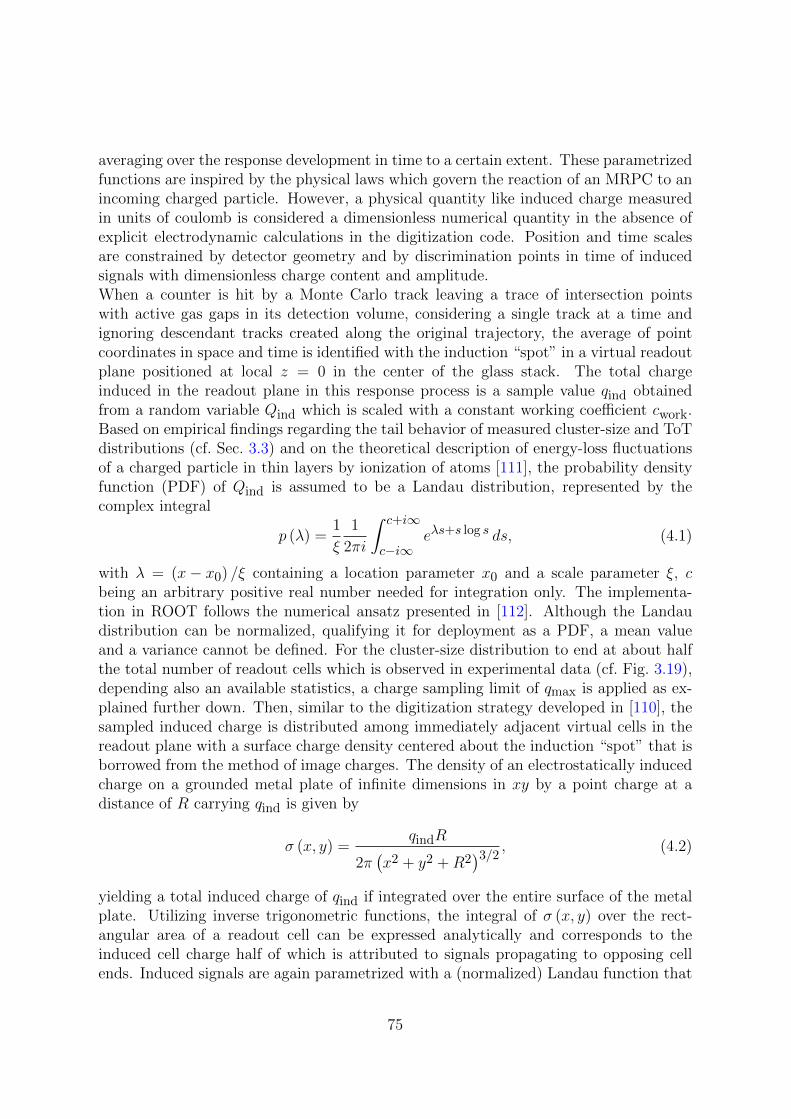
averaging over the response development in time to a certain extent. These parametrizedfunctions are inspired by the physical laws which govern the reaction of an MRPC to anincoming charged particle. However, a physical quantity like induced charge measuredin units of coulomb is considered a dimensionless numerical quantity in the absence ofexplicit electrodynamic calculations in the digitization code. Position and time scalesare constrained by detector geometry and by discrimination points in time of inducedsignals with dimensionless charge content and amplitude.When a counter is hit by a Monte Carlo track leaving a trace of intersection pointswith active gas gaps in its detection volume, considering a single track at a time andignoring descendant tracks created along the original trajectory, the average of pointcoordinates in space and time is identified with the induction “spot” in a virtual readoutplane positioned at local z = 0 in the center of the glass stack. The total chargeinduced in the readout plane in this response process is a sample value qind obtainedfrom a random variable Qind which is scaled with a constant working coefficient cwork.Based on empirical findings regarding the tail behavior of measured cluster-size and ToTdistributions (cf. Sec. 3.3) and on the theoretical description of energy-loss fluctuationsof a charged particle in thin layers by ionization of atoms [111], the probability densityfunction (PDF) of Qind is assumed to be a Landau distribution, represented by thecomplex integral

p (λ) =1

ξ

1

2πi

∫ c+i∞

c−i∞eλs+s log s ds, (4.1)

with λ = (x− x0) /ξ containing a location parameter x0 and a scale parameter ξ, cbeing an arbitrary positive real number needed for integration only. The implementa-tion in ROOT follows the numerical ansatz presented in [112]. Although the Landaudistribution can be normalized, qualifying it for deployment as a PDF, a mean valueand a variance cannot be defined. For the cluster-size distribution to end at about halfthe total number of readout cells which is observed in experimental data (cf. Fig. 3.19),depending also an available statistics, a charge sampling limit of qmax is applied as ex-plained further down. Then, similar to the digitization strategy developed in [110], thesampled induced charge is distributed among immediately adjacent virtual cells in thereadout plane with a surface charge density centered about the induction “spot” that isborrowed from the method of image charges. The density of an electrostatically inducedcharge on a grounded metal plate of infinite dimensions in xy by a point charge at adistance of R carrying qind is given by

σ (x, y) =qindR

2π(x2 + y2 +R2

)3/2 , (4.2)

yielding a total induced charge of qind if integrated over the entire surface of the metalplate. Utilizing inverse trigonometric functions, the integral of σ (x, y) over the rect-angular area of a readout cell can be expressed analytically and corresponds to theinduced cell charge half of which is attributed to signals propagating to opposing cellends. Induced signals are again parametrized with a (normalized) Landau function that

75

is multiplied with the numerical charge content,

f (t) =qcell

2× Landau (t, t0, ξt) , (4.3)

positioned on the time axis—for numerical reasons—with a fixed offset t0 (here: 14 ns)and scaled with a free model parameter ξt which is—once determined—used unal-teredly for all signals generated, i.e. only the charge coefficient varies between signals(cf. Fig. 3.20 for a visualization). A Landau function was chosen primarily in viewof approximately reproducing the shape of measured ToT spectra which could not beachieved with triangular or exponentially rising/falling signal functions.Skipping the preamplification stage for simplicity which deprives the model—at themoment—of considering gain differences between PADI channels, the maximum ampli-tudes of parametrized signals induced on every counter cell (with varying charge contentdepending on the distance of the respective cell to the induction point) are checkedagainst a numerical discrimination threshold at each cell end. This dimensionless quan-tity is yet another free model parameter. As the same underlying Landau parametriza-tion is applied to all signals, the function maximum linked to the most probable valueof the distribution needs to be determined by numerical minimization only once at thebeginning of the digitization run. Multiplying this maximum value with the respectivecharge content allows for a quick assessment whether a cell signal is above thresholdor can be disregarded. In the former case, leading- and trailing-edge discriminationpoints in time, i.e. the two intersections between the signal and a constant threshold,are evaluated numerically utilizing one-dimensional root-finding methods provided bythe GNU Scientific Library (GSL). To the time difference between signal edges a freeToT offset parameter is added to give some additional flexibility to the optimizationalgorithm. Revisiting the aforementioned charge sampling limit of qmax in the light ofcharge spreading and signal discrimination, it is determined such that, placing the in-duction point in the xy-center of the counter with the aim of obtaining nmax/2 efficientcells in both directions, the corresponding signal induced on cell ± (nmax/2 + 1) countedfrom the center does not exceed threshold anymore. If this limit holds for an inductionpoint in the counter center relatively yielding the largest charge shares by surface inte-gration, then it is universally applicable to any point in the readout plane.At this level in the simulated response process for an individual MC track, both clustersize and efficiency are known and not subject to change anymore, the former quantitycounting the number of readout cells on which a measurable signal was induced, indepen-dent of matching criteria for reconstructed cell hits in time and position (cf. Sec. 3.3),and the latter value registering if any cell exhibited a signal above threshold. In theabsence of gain variations between preamplifier channels (and dispersion effects whichcould possibly cause signals to arrive at opposing cell ends with amplitudes differing fromeach other), signals exceed threshold either on both cell ends or on none. An exemplarysimulated cluster-size spectrum for counter 9-0-0 is shown in Fig. 4.1. Compared to themeasured spectrum in Fig. 3.19, the difference in relative frequencies between two-celland three-cell clusters is larger in the simulated case and the spectrum has a more log-arithmically convex appearance.

76

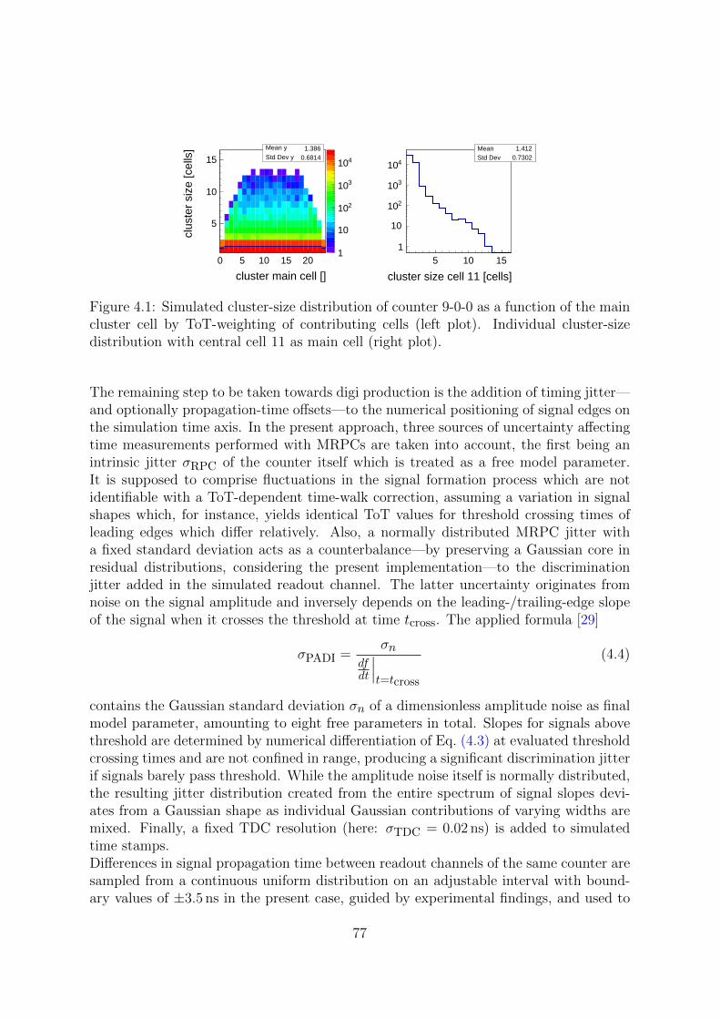
0 5 10 15 20

cluster main cell []

5

10

15

clu

ster

siz

e [c

ells

]

1

10

210

310

410

Mean y 1.386Std Dev y 0.6814

Mean 1.412Std Dev 0.7302

5 10 15

cluster size cell 11 [cells]

1

10

210

310

410

Mean 1.412Std Dev 0.7302

Figure 4.1: Simulated cluster-size distribution of counter 9-0-0 as a function of the maincluster cell by ToT-weighting of contributing cells (left plot). Individual cluster-sizedistribution with central cell 11 as main cell (right plot).

The remaining step to be taken towards digi production is the addition of timing jitter—and optionally propagation-time offsets—to the numerical positioning of signal edges onthe simulation time axis. In the present approach, three sources of uncertainty affectingtime measurements performed with MRPCs are taken into account, the first being anintrinsic jitter σRPC of the counter itself which is treated as a free model parameter.It is supposed to comprise fluctuations in the signal formation process which are notidentifiable with a ToT-dependent time-walk correction, assuming a variation in signalshapes which, for instance, yields identical ToT values for threshold crossing times ofleading edges which differ relatively. Also, a normally distributed MRPC jitter witha fixed standard deviation acts as a counterbalance—by preserving a Gaussian core inresidual distributions, considering the present implementation—to the discriminationjitter added in the simulated readout channel. The latter uncertainty originates fromnoise on the signal amplitude and inversely depends on the leading-/trailing-edge slopeof the signal when it crosses the threshold at time tcross. The applied formula [29]

σPADI =σn

dfdt

∣∣∣t=tcross

(4.4)

contains the Gaussian standard deviation σn of a dimensionless amplitude noise as finalmodel parameter, amounting to eight free parameters in total. Slopes for signals abovethreshold are determined by numerical differentiation of Eq. (4.3) at evaluated thresholdcrossing times and are not confined in range, producing a significant discrimination jitterif signals barely pass threshold. While the amplitude noise itself is normally distributed,the resulting jitter distribution created from the entire spectrum of signal slopes devi-ates from a Gaussian shape as individual Gaussian contributions of varying widths aremixed. Finally, a fixed TDC resolution (here: σTDC = 0.02 ns) is added to simulatedtime stamps.Differences in signal propagation time between readout channels of the same counter aresampled from a continuous uniform distribution on an adjustable interval with bound-ary values of ±3.5 ns in the present case, guided by experimental findings, and used to

77

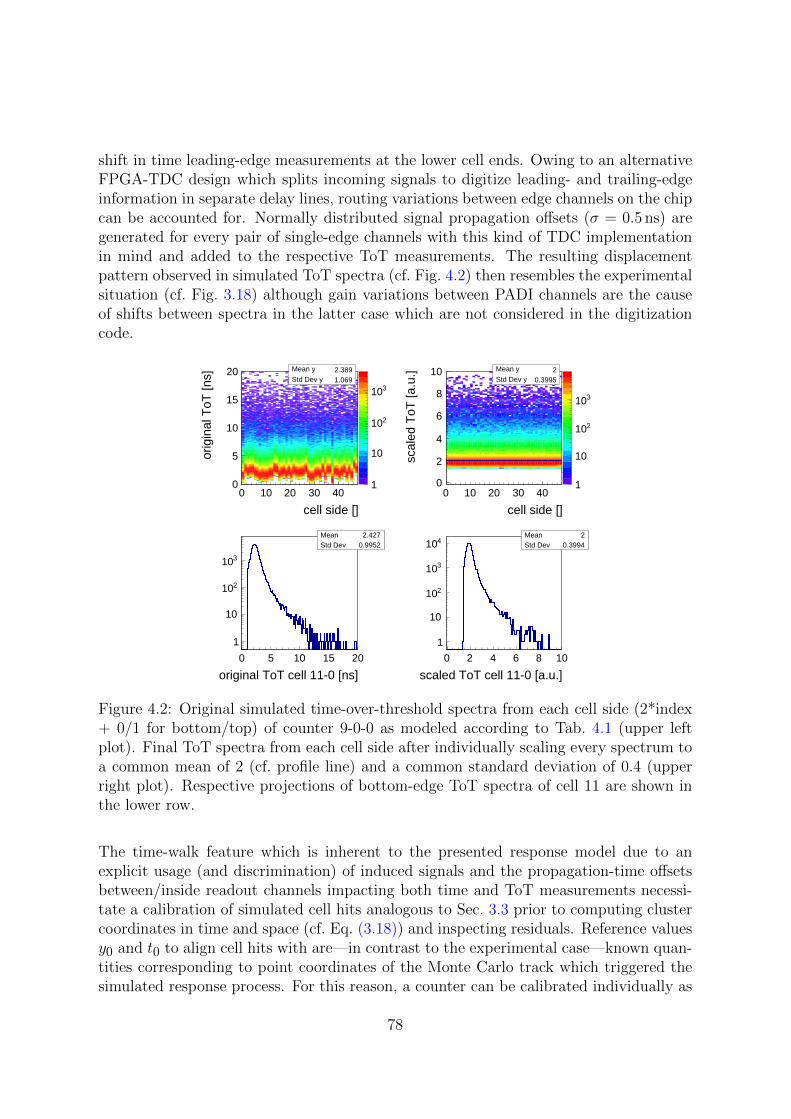
shift in time leading-edge measurements at the lower cell ends. Owing to an alternativeFPGA-TDC design which splits incoming signals to digitize leading- and trailing-edgeinformation in separate delay lines, routing variations between edge channels on the chipcan be accounted for. Normally distributed signal propagation offsets (σ = 0.5 ns) aregenerated for every pair of single-edge channels with this kind of TDC implementationin mind and added to the respective ToT measurements. The resulting displacementpattern observed in simulated ToT spectra (cf. Fig. 4.2) then resembles the experimentalsituation (cf. Fig. 3.18) although gain variations between PADI channels are the causeof shifts between spectra in the latter case which are not considered in the digitizationcode.

0 10 20 30 40

cell side []

0

5

10

15

20

orig

inal

ToT

[ns]

1

10

210

310

Mean y 2.389Std Dev y 1.069

0 10 20 30 40

cell side []

0

2

4

6

8

10

sca

led

ToT

[a.u

.]

1

10

210

310

Mean y 2Std Dev y 0.3995

Mean 2.427Std Dev 0.9952

0 5 10 15 20

original ToT cell 11-0 [ns]

1

10

210

310

Mean 2.427Std Dev 0.9952

Mean 2Std Dev 0.3994

0 2 4 6 8 10

scaled ToT cell 11-0 [a.u.]

1

10

210

310

410Mean 2Std Dev 0.3994

Figure 4.2: Original simulated time-over-threshold spectra from each cell side (2*index+ 0/1 for bottom/top) of counter 9-0-0 as modeled according to Tab. 4.1 (upper leftplot). Final ToT spectra from each cell side after individually scaling every spectrum toa common mean of 2 (cf. profile line) and a common standard deviation of 0.4 (upperright plot). Respective projections of bottom-edge ToT spectra of cell 11 are shown inthe lower row.

The time-walk feature which is inherent to the presented response model due to anexplicit usage (and discrimination) of induced signals and the propagation-time offsetsbetween/inside readout channels impacting both time and ToT measurements necessi-tate a calibration of simulated cell hits analogous to Sec. 3.3 prior to computing clustercoordinates in time and space (cf. Eq. (3.18)) and inspecting residuals. Reference valuesy0 and t0 to align cell hits with are—in contrast to the experimental case—known quan-tities corresponding to point coordinates of the Monte Carlo track which triggered thesimulated response process. For this reason, a counter can be calibrated individually as

78

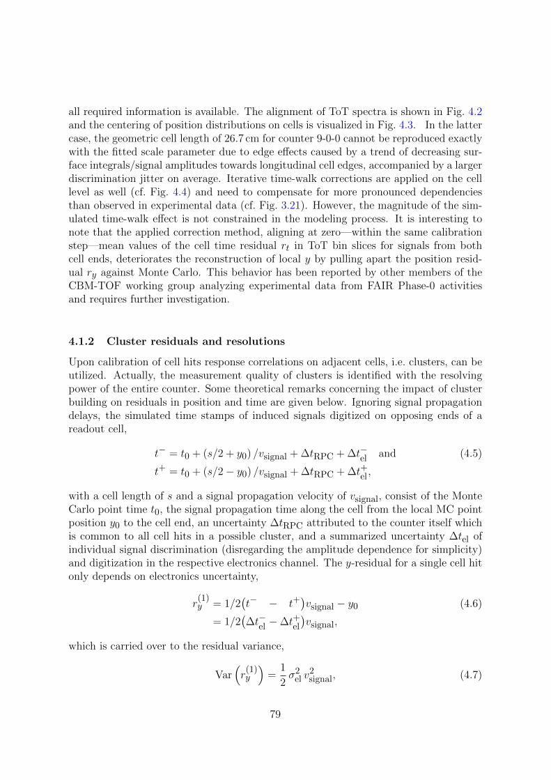
all required information is available. The alignment of ToT spectra is shown in Fig. 4.2and the centering of position distributions on cells is visualized in Fig. 4.3. In the lattercase, the geometric cell length of 26.7 cm for counter 9-0-0 cannot be reproduced exactlywith the fitted scale parameter due to edge effects caused by a trend of decreasing sur-face integrals/signal amplitudes towards longitudinal cell edges, accompanied by a largerdiscrimination jitter on average. Iterative time-walk corrections are applied on the celllevel as well (cf. Fig. 4.4) and need to compensate for more pronounced dependenciesthan observed in experimental data (cf. Fig. 3.21). However, the magnitude of the sim-ulated time-walk effect is not constrained in the modeling process. It is interesting tonote that the applied correction method, aligning at zero—within the same calibrationstep—mean values of the cell time residual rt in ToT bin slices for signals from bothcell ends, deteriorates the reconstruction of local y by pulling apart the position resid-ual ry against Monte Carlo. This behavior has been reported by other members of theCBM-TOF working group analyzing experimental data from FAIR Phase-0 activitiesand requires further investigation.

4.1.2 Cluster residuals and resolutions

Upon calibration of cell hits response correlations on adjacent cells, i.e. clusters, can beutilized. Actually, the measurement quality of clusters is identified with the resolvingpower of the entire counter. Some theoretical remarks concerning the impact of clusterbuilding on residuals in position and time are given below. Ignoring signal propagationdelays, the simulated time stamps of induced signals digitized on opposing ends of areadout cell,

t− = t0 + (s/2 + y0) /vsignal + ∆tRPC + ∆t−el and (4.5)

t+ = t0 + (s/2− y0) /vsignal + ∆tRPC + ∆t+el ,

with a cell length of s and a signal propagation velocity of vsignal, consist of the MonteCarlo point time t0, the signal propagation time along the cell from the local MC pointposition y0 to the cell end, an uncertainty ∆tRPC attributed to the counter itself whichis common to all cell hits in a possible cluster, and a summarized uncertainty ∆tel ofindividual signal discrimination (disregarding the amplitude dependence for simplicity)and digitization in the respective electronics channel. The y-residual for a single cell hitonly depends on electronics uncertainty,

r(1)y = 1/2

(t− − t+

)vsignal − y0 (4.6)

= 1/2(∆t−el −∆t+el

)vsignal,

which is carried over to the residual variance,

Var(r

(1)y

)=

1

2σ2

el v2signal, (4.7)

79

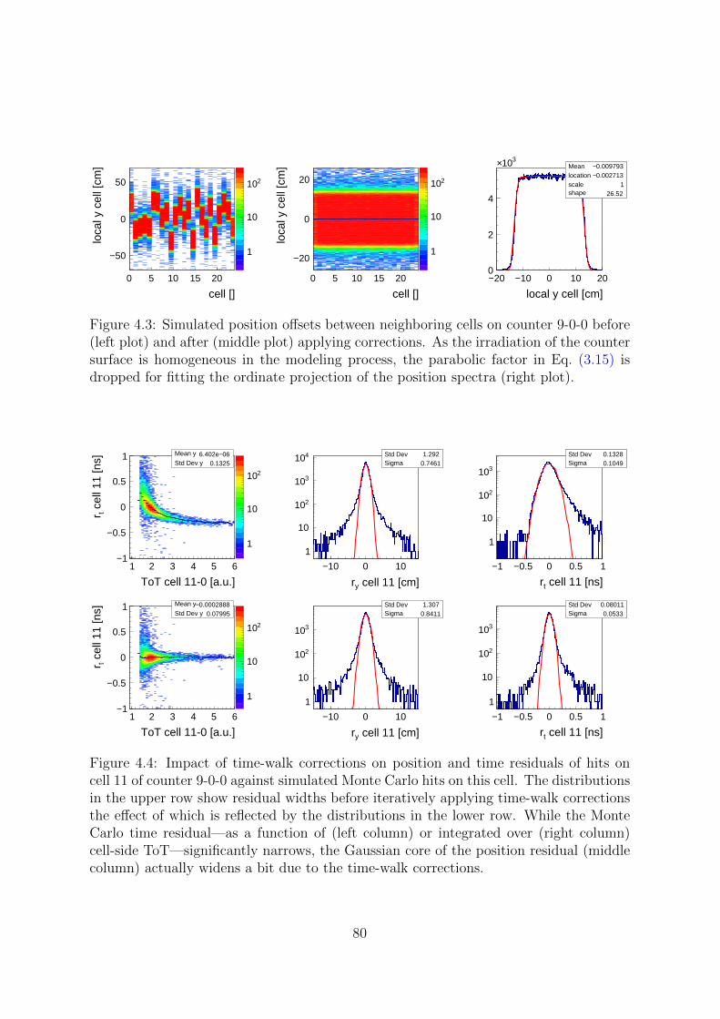
0 5 10 15 20

cell []

50−

0

50

loca

l y c

ell [

cm]

1

10

210

0 5 10 15 20

cell []

20−

0

20

loca

l y c

ell [

cm]

1

10

210

Mean 0.009793− location 0.002713− scale 1shape 26.52

20− 10− 0 10 20

local y cell [cm]

0

2

4

310× Mean 0.009793− location 0.002713− scale 1shape 26.52

Figure 4.3: Simulated position offsets between neighboring cells on counter 9-0-0 before(left plot) and after (middle plot) applying corrections. As the irradiation of the countersurface is homogeneous in the modeling process, the parabolic factor in Eq. (3.15) isdropped for fitting the ordinate projection of the position spectra (right plot).

1 2 3 4 5 6

ToT cell 11-0 [a.u.]

1−

0.5−

0

0.5

1

cel

l 11

[ns]

t r

1

10

210

Mean y 06− 6.402eStd Dev y 0.1325

Std Dev 1.292Sigma 0.7461

10− 0 10

cell 11 [cm]y r

1

10

210

310

410 Std Dev 1.292Sigma 0.7461

Std Dev 0.1328Sigma 0.1049

1− 0.5− 0 0.5 1

cell 11 [ns]t r

1

10

210

310

Std Dev 0.1328Sigma 0.1049

1 2 3 4 5 6

ToT cell 11-0 [a.u.]

1−

0.5−

0

0.5

1

cel

l 11

[ns]

t r

1

10

210

Mean y 0.0002888− Std Dev y 0.07995

Std Dev 1.307Sigma 0.8411

10− 0 10

cell 11 [cm]y r

1

10

210

310

Std Dev 1.307Sigma 0.8411

Std Dev 0.08011Sigma 0.0533

1− 0.5− 0 0.5 1

cell 11 [ns]t r

1

10

210

310

Std Dev 0.08011Sigma 0.0533

Figure 4.4: Impact of time-walk corrections on position and time residuals of hits oncell 11 of counter 9-0-0 against simulated Monte Carlo hits on this cell. The distributionsin the upper row show residual widths before iteratively applying time-walk correctionsthe effect of which is reflected by the distributions in the lower row. While the MonteCarlo time residual—as a function of (left column) or integrated over (right column)cell-side ToT—significantly narrows, the Gaussian core of the position residual (middlecolumn) actually widens a bit due to the time-walk corrections.

80

denoting equal Var (∆tel) for both readout channels with σ2el to indicate the link to the

standard deviation. In the time residual, the intrinsic uncertainty of the MRPC doesnot cancel out when adding signal time stamps,

r(1)t = 1/2

(t− + t+

)− 1/2 s/vsignal − t0 (4.8)

= ∆tRPC + 1/2(∆t−el + ∆t+el

),

and constitutes a second contribution to the residual width,

Var(r

(1)t

)= σ2

RPC +1

2σ2

el, (4.9)

expressing Var (∆tRPC) in terms of σRPC. If multiple cell hits are grouped into an n-cellresponse cluster, the passage of a charged particle through the detector was registered byn independent measuring devices in a way, the respective results of which are weightedwith time over threshold to obtain cluster coordinates. Here, for the mathematicalargument, equal weighting of cell measurements with wi = 1/n is assumed. The positionresidual in local y of a cluster with n cells can be reduced to

r(n)y =

1

2

1

n

n∑i=1

(∆t

(i)−el −∆t

(i)+el

)vsignal (4.10)

and has a vanishing variance in the limit n→∞,

Var(r

(n)y

)=

1

2

1

nσ2

el v2signal. (4.11)

In time, the intrinsic MRPC uncertainty is preserved,

r(n)t = ∆tRPC +

1

2

1

n

n∑i=1

(∆t

(i)−el + ∆t

(i)+el

), (4.12)

and the variance asymptotically approaches σRPC for increasing cluster sizes,

Var(r

(n)t

)= σ2

RPC +1

2

1

nσ2

el. (4.13)

Aiming at a reduction of the statistical error of measurement, large clusters are favorablein comparison to small clusters. However, designing an MRPC with a highly granularreadout electrode consisting of many small cells increases the demand for costly electron-ics channels. Clusters comprising a multitude of cells are also predisposed to responseinterference of different tracks. The fewer clean signals are required for a measurement,the better the device performs on average despite of statistical considerations.Regarding residuals in local x, the single-cell case is equivalent to a continuous uniformdistribution across the readout cell of width sx with a variance of

Var(r

(1)x

)=s2x

12. (4.14)

81

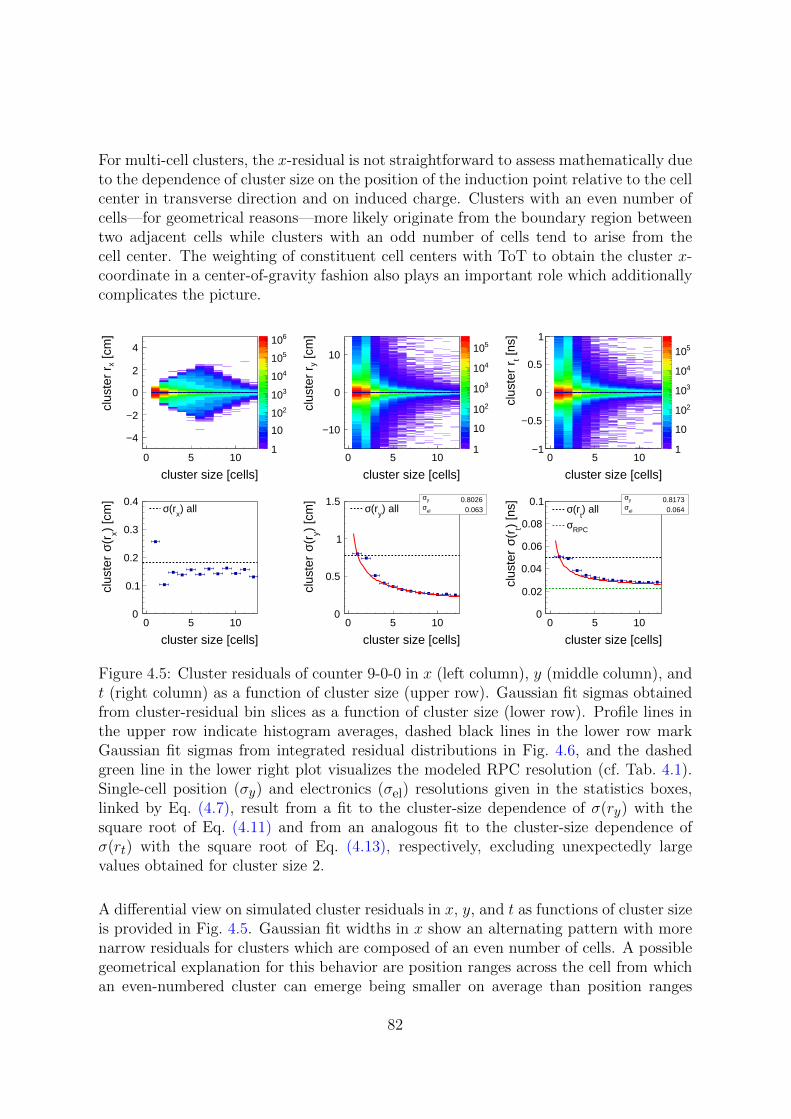
For multi-cell clusters, the x-residual is not straightforward to assess mathematically dueto the dependence of cluster size on the position of the induction point relative to the cellcenter in transverse direction and on induced charge. Clusters with an even number ofcells—for geometrical reasons—more likely originate from the boundary region betweentwo adjacent cells while clusters with an odd number of cells tend to arise from thecell center. The weighting of constituent cell centers with ToT to obtain the cluster x-coordinate in a center-of-gravity fashion also plays an important role which additionallycomplicates the picture.

0 5 10

cluster size [cells]

4−

2−

0

2

4

[cm

]x

clu

ster

r

1

10

210

310

410

510

610

0 5 10

cluster size [cells]

10−

0

10 [cm

]y

clu

ster

r

1

10

210

310

410

510

0 5 10

cluster size [cells]

1−

0.5−

0

0.5

1

[ns]

t c

lust

er r

1

10

210

310

410

510

0 5 10

cluster size [cells]

0

0.1

0.2

0.3

0.4

) [c

m]

x(rσ

clu

ster

) allx

(rσ yσ 0.8026

elσ 0.063

0 5 10

cluster size [cells]

0

0.5

1

1.5

) [c

m]

y(rσ

clu

ster

) ally

(rσ yσ 0.8173

elσ 0.064

0 5 10

cluster size [cells]

0

0.02

0.04

0.06

0.08

0.1)

[ns]

t(rσ

clu

ster

) allt

(rσ

RPCσ

Figure 4.5: Cluster residuals of counter 9-0-0 in x (left column), y (middle column), andt (right column) as a function of cluster size (upper row). Gaussian fit sigmas obtainedfrom cluster-residual bin slices as a function of cluster size (lower row). Profile lines inthe upper row indicate histogram averages, dashed black lines in the lower row markGaussian fit sigmas from integrated residual distributions in Fig. 4.6, and the dashedgreen line in the lower right plot visualizes the modeled RPC resolution (cf. Tab. 4.1).Single-cell position (σy) and electronics (σel) resolutions given in the statistics boxes,linked by Eq. (4.7), result from a fit to the cluster-size dependence of σ(ry) with thesquare root of Eq. (4.11) and from an analogous fit to the cluster-size dependence ofσ(rt) with the square root of Eq. (4.13), respectively, excluding unexpectedly largevalues obtained for cluster size 2.

A differential view on simulated cluster residuals in x, y, and t as functions of cluster sizeis provided in Fig. 4.5. Gaussian fit widths in x show an alternating pattern with morenarrow residuals for clusters which are composed of an even number of cells. A possiblegeometrical explanation for this behavior are position ranges across the cell from whichan even-numbered cluster can emerge being smaller on average than position ranges

82

for generating odd-numbered clusters, reducing the uncertainty interval between MonteCarlo point and cluster position and, hence, constricting the residual. For a single-cell cluster, the fit value is below the theoretical expectation of 0.29 cm calculated withEq. (4.14) for a 1 cm wide cell because of an increasing probability for two-cell clusterproduction towards the cell periphery, rounding off the edges of the originally uniformdistribution, and due to fitting the latter with a Gaussian function. Residual widths in yand in t generally follow the functional relations to cluster size derived above, except fortwo-cell clusters owing to an extraordinarily small mean amplitude and slope (revisitedbelow) of the four measured signals which resemble each other to a higher degree thanis the case for any other cluster size, excluding single-cell clusters. Thus, four similarmeasurements with a relatively high discrimination uncertainty each accumulate.The single-channel electronics resolution σel which is extracted from fits to residualwidths in local y and in time indirectly, i.e. via the amplitude noise σn (cf. Eq. (4.4)),is a free model parameter like the intrinsic RPC resolution σRPC. During parameteradjustment, the relative weighting between both quantities arises from constraints puton the integrated cluster time resolution, at a nominal working coefficient of 1.5 onthe one hand and in a degraded situation associated with an efficiency drop to 80 %on the other hand. As the contribution of σRPC to residual widths remains constant,in the current implementation at least, the deterioration of the timing response with adecreasing working coefficient which translates into smaller signals on average is solelydriven by a corresponding increase in discrimination jitter. Thus, an unrealisticallypoor electronics resolution of about 0.063 ns tied to a single-cell y-position resolution of0.8 cm is obtained (here for counter 9-0-0) to comply with modeling constraints, whilethe intrinsic MRPC resolution amounts to 0.024 ns. A mitigation of this effect couldbe accomplished by coupling σRPC to cwork, taking load off σn concerning responsedeterioration. Increasing σRPC while keeping the cluster time resolution fixed thenleads to an improved resolution in y, according to

Var(ry)

=(

Var (rt)− σ2RPC

)v2

signal. (4.15)

To estimate the average response of the counter to incoming particles, cluster residualsintegrated over cluster size are considered and fitted with Gaussian functions to obtainresidual widths which are identified with the resolution in the respective response dimen-sion (cf. Fig. 4.6). By merging results for individual cluster sizes in a single histogram,however, mixture distributions are generated which are technically not Gaussian in shapealthough the underlying residuals for a specified cluster size are normally distributed, ne-glecting the amplitude dependence of the discrimination jitter. In the simplified picturedescribed above, the theoretical mixture variances of the integrated y-residual,

Var(ry)

=∞∑n=1

pnVar(r

(n)y

)(4.16)

=1

2σ2

el v2signal

∞∑n=1

pnn,

83

and of the integrated t-residual,

Var (rt) =∞∑n=1

pnVar(r

(n)t

)(4.17)

= σ2RPC +

1

2σ2

el

∞∑n=1

pnn,

both depend on the inverse weighted harmonic mean of the cluster-size distribution, ex-pressed by the infinite sum over inverse cluster sizes n weighted with relative frequenciespn.

Std Dev 0.2098Sigma 0.1824

4− 2− 0 2 4

[cm]x cluster r

1

10

210

310

410

Std Dev 0.2098Sigma 0.1824

Std Dev 1.015Sigma 0.7788

10− 0 10

[cm]y cluster r

1

10

210

310

410 Std Dev 1.015Sigma 0.7788

Std Dev 0.06288Sigma 0.04997

1− 0.5− 0 0.5 1

[ns]t cluster r

1

10

210

310

410Std Dev 0.06288Sigma 0.04997

Std Dev 0.2095Sigma 0.09895

1− 0 1

[cm]x cluster r

0

10

20

310× Std Dev 0.2095Sigma 0.09895

Std Dev 0.9293Sigma 0.7108

5− 0 5

[cm]y cluster r

0

2

4

310× Std Dev 0.9293Sigma 0.7108

Std Dev 0.05793Sigma 0.04724

0.5− 0 0.5

[ns]t cluster r

0

2

4

6

8

310× Std Dev 0.05793Sigma 0.04724

Figure 4.6: Time-walk corrected residuals in x (left column), y (middle column), andt (right column) between ideal cell clusters and the corresponding Monte Carlo pointson the surface of counter 9-0-0, in logarithmic (upper row) and in linear scale (lowerrow). Differences between widths of Gaussian fits to the entire distribution (upper row)and widths of Gaussian fits to the distribution peaks only (lower row) cannot only beattributed to non-Gaussian tails ascribable to discrimination jitter which affects ry andrt but also to the inherent mixture character of distributions containing residuals fromthe entire spectrum of cluster sizes. The x-residual which is a simple uniform distributionfor a cluster of size 1 (cf. Eq. (4.14)) and which receives its final shape from ToT-weightedcenters of cells contributing to a multi-cell cluster is anyway not intrinsically Gaussian.

The corresponding standard deviations differ numerically from Gaussian sigmas obtainedby fitting residuals. However, the latter values are the best estimators available for the“Gaussicity” of the response residual in each dimension and serve as weights to a χ2-formalism which is applied to matching residuals between counters in the final analysis

84

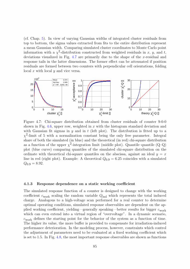
(cf. Chap. 5). In view of varying Gaussian widths of integrated cluster residuals fromtop to bottom, the sigma values extracted from fits to the entire distribution representa mean Gaussian width. Comparing simulated cluster coordinates to Monte Carlo pointinformation with a χ2-distribution constructed from weighted residuals in x, y, and t,deviations visualized in Fig. 4.7 are primarily due to the shape of the x-residual andresponse tails in the latter dimensions. The former effect can be attenuated if positionresiduals are formed between two counters with perpendicular cell orientations, foldinglocal x with local y and vice versa.

Mean 3.374Std Dev 2.909

/ ndf 2χ 5245 / 49

0 5 10 15

[]32χ cluster

0

5

10

15

20

310× Mean 3.374Std Dev 2.909

/ ndf 2χ 5245 / 49

0 10 20 30

-limit []32χ

0.5

0.6

0.7

0.8

0.9

1

-acc

epta

nce

[]32 χ

0 10 20 30

-Q []32χ theory

0

10

20

30

-Q []

32 χ c

lust

er

Figure 4.7: Chi-square distribution obtained from cluster residuals of counter 9-0-0shown in Fig. 4.6, upper row, weighted in x with the histogram standard deviation andwith Gaussian fit sigmas in y and in t (left plot). The distribution is fitted up to aχ2-limit of 5 with a normalization constant being the only free parameter. Integralshare of both the simulated (in blue) and the theoretical (in red) chi-square distributionas a function of the upper χ2-integration limit (middle plot). Quantile–quantile (Q–Q)plot (blue curve) comparing quantiles of the simulated chi-square distribution on theordinate with theoretical chi-square quantiles on the abscissa, against an ideal y = xline in red (right plot). Example: A theoretical Q0.9 = 6.25 coincides with a simulatedQ0.9 = 8.92.

4.1.3 Response dependence on a static working coefficient

The simulated response function of a counter is designed to change with the workingcoefficient cwork scaling the random variable Qind which represents the total inducedcharge. Analogous to a high-voltage scan performed for a real counter to determineoptimal operating conditions, simulated response observables are dependent on the ap-plied working coefficient, yielding—generally speaking—better results for bigger cworkwhich can even extend into a virtual region of “overvoltage”. In a dynamic scenario,cwork defines the starting point for the behavior of the system as a function of time.The higher its value, the more buffer is provided to compensate for irradiation-inducedperformance deterioration. In the modeling process, however, constraints which controlthe adjustment of parameters need to be evaluated at a fixed working coefficient whichis set to 1.5. In Fig. 4.8, the most important response observables are shown as functions

85

[]work c

0

0.5

1

det

ectio

n ef

ficie

ncy

[] -kneeε = 0.8ε-flexε

00.511.5

[]work c

1

1.2

1.4

1.6

1.8

2

mea

n cl

uste

r si

ze [c

ells

]

= 0.8ε-flexε

00.511.5

[]work c

1.6

1.8

2

2.2

2.4

mea

n T

oT c

ell 1

1-0

[a.u

.] = 0.8ε-flexε

00.511.5

[]work c

0

0.1

0.2

0.3

0.4

0.5

) [c

m]

x(rσ

clu

ster

= 0.8ε-flexε

00.511.5

[]work c

0

0.5

1

1.5

2

) [c

m]

y(rσ

clu

ster

= 0.8ε-flexε

00.511.5

[]work c

0

0.05

0.1

0.15

) [n

s]t

(rσ c

lust

er

= 0.8ε-flexε

00.511.5

Figure 4.8: Evolution of the Monte Carlo detection efficiency (upper left plot), the meancluster size (upper middle plot), an exemplary mean channel ToT (upper right plot),and the residual sigmas in x (lower left plot), y (lower middle plot), and t (lower rightplot) on counter 9-0-0 as a function of working coefficient cwork which the accessibleinduced charge spectrum is (down-)scaled with. The efficiency evolution is fitted withthe logistic sigmoid function from Eq. (4.18). As points of orientation, the efficiency-knee coefficient (cwork = 1.0), the degradation coefficient (ε = 0.8), and the sigmoidalinflection coefficient (cwork ≈ 0.5) are indicated by colored dashed lines. The trendreversal in observables towards smaller values of cwork at about the inflection coefficientis discussed in the text.

of cwork. Concerning detection efficiency, the idea to fit the curve with a logistic sigmoidfunction,

f(x) = a+d

1 + e−λ(x−x0), (4.18)

and to use the label “efficiency knee” for the point at which the efficiency reaches 95 % aretaken from [113]. The S-curve formula comprises an offset a, the distance d between thetwo asymptotes, the mid- or inflection point x0, and the efficiency slope at x0 multipliedby 4/d, which is λ. Two constraints to be met by the free model parameters are derivedfrom this function, the first one positioning the “knee” at cwork = 1.0 and the latterone requiring d to equal 1. In addition, a reference value for the degradation of timingperformance is associated with an efficiency drop to 80 % in view of a dynamic scenariodiscussed in Sec. 4.2. Except for efficiency and x-residual width, all curves exhibit atrend reversal with decreasing cwork which roughly occurs at the flex coefficient of theefficiency sigmoid. This effect is caused by the tail of the Landau distribution which the

86

total induced charge is sampled from. If analytic Landau approximations like Gumbelor Moyal distributions are used instead, this behavior is not observed but the shapeof experimental cluster-size and ToT distributions cannot be reproduced with thesesubstitutes due to their less pronounced tails. For this reason, the Landau solution ismaintained which allows for studying the response deterioration in the efficiency rangeabove ∼ 50 % before the counterintuitive response improvement sets in. Actually, thebehavior of mean cluster size in a high-voltage scan conducted with MRPCs deployedat the CMS experiment [114] suggests to experimentally investigate the region beyondefficiency inflection with sufficient statistics. When the working coefficient approacheszero, a second trend reversal reflects the rapidly decreasing probability to generate multi-cell clusters with the limited induced charge spectrum still available.

4.1.4 Parameter adjustment and model limitations

To adjust the response parameters of the diamond detector and four MRPCs in the setupat CERN/SPS, five parameter sets need to be generated for five different readout-cellgeometries. The reference values of the selected boundary conditions which constrainthe modeling process (cf. Tab. 4.1) are deduced from experimental observations and—inthis work—chosen to be identical for all counters. If special response characteristics ofindividual detectors need to be considered, individual values can be applied which neces-sitates a readjustment of model parameters. The diamond is treated as a small MRPCfor simplicity. To complement information on the listed constraints, the ratio betweenroot mean square and Gaussian sigma obtained for the y-residual is supposed to regu-late the impact of discimination jitter without directly posing a condition on the residualwidth in y which would conflict with the target value for σ (rt) as resolutions in y andt are mutually dependent. The degraded cluster time resolution of 0.070 ns is an upperstability limit for a parametrization which bases timing deterioration on the increasingdiscrimination jitter for diminishing signal amplitudes only; experimental results indicatelarger deteriorations at 80 % detection efficiency (cf. Sec. 4.2). Parameters are optimizednumerically utilizing a GSL implementation of the downhill simplex algorithm [115] byminimizing a chi-square constructed from weighted differences, depending on the de-sired precision, between reference values and response observables obtained with thecurrent parameter set. As the digitization code intrinsically generates non-ideal signaltime stamps and shifted ToT spectra which require offset, scaling, and time-walk cor-rections to be applied, the chi-square calculation in every single iteration of the simplexalgorithm—upon modifying a model parameter—is preceded by five iterations of countercalibration against Monte Carlo information at the nominal working coefficient of 1.5.Moreover, concerning constraints imposed on efficiency and time-residual deterioration,the response is subsequently evaluated for a total of 15 working coefficients between 1.5and 0, for every minimization step. The calibration of reconstructed cell hits obtainedfor cwork = 1.5 can be reused throughout the entire range of working coefficients. A sin-gle response evaluation is based on one million Monte Carlo points which are uniformlydistributed in the virtual readout plane of the counter. Thus, the time it takes for the

87

Table 4.1: Reference values and their reproduction (at cwork = 1.5 if not stated other-wise) with the five different counter geometries in the setup (upper part) constrainingthe adjustment of free parameters for response modeling (middle part). The values ofsome observables resulting from the parametrization are given in the lower part of thetable. For details see text.

ref. 5-1-0 3-0-0 9-0-0 7-0-0 4-0-0

mean cluster size central cell [cells] 1.4 1.438 1.358 1.412 1.332 1.361

cluster-size RMS central cell [cells] 0.7 0.698 0.688 0.730 0.591 0.619

mean ToT central cell [ns] 2.5 2.553 2.586 2.427 2.685 2.550

ToT RMS central cell [ns] 1.0 1.035 0.776 0.999 0.776 0.996

cluster σ(rt) [ns] 0.050 0.050 0.050 0.050 0.050 0.050

cluster RMS(ry)/σ(ry) ratio 0.75 0.763 0.785 0.767 0.794 0.765

sigmoidal knee efficiency (cwork = 1.0) 0.95 0.935 0.943 0.949 0.949 0.934

sigmoidal efficiency drop 1.0 1.028 0.993 1.047 1.004 1.053

degraded (ε = 0.8) cluster σ(rt) [ns] 0.070 0.073 0.081 0.073 0.079 0.071

induced-charge Landau location [a.u.] n/a 5.916 4.042 4.000 4.163 4.609

induced-charge Landau scale [a.u.] n/a 1.065 0.421 0.761 0.518 0.811

surface-charge-density distance [cm] n/a 0.027 0.226 0.184 0.387 0.170

induced-signal Landau scale [ns] n/a 0.324 0.250 0.263 0.259 0.272

discrimination threshold [a.u.] n/a 0.757 0.689 0.620 0.682 0.670

induced-signal ToT offset [ns] n/a 0.877 1.412 0.966 1.402 1.079

amplitude jitter σn [a.u.] n/a 0.193 0.204 0.197 0.206 0.193

avalanche jitter σRPC [ns] n/a 0.020 0.024 0.023 0.023 0.025

cluster σ(rx) [cm] n/a 0.019 0.169 0.182 0.348 0.166

cluster σ(ry) [cm] n/a 0.805 0.765 0.779 0.772 0.751

minimization algorithm to converge to a stable solution in parameter space can amountto up to 24 hours.Apart from the imbalance between intrinsic MRPC and discrimination types of jitterowing to the constancy of the former with decreasing working coefficients (cf. Sec. 4.1.2),the presented digitization approach is primarily subject to bias originating from a heavy-tailed Landau distribution used for induced-charge sampling (cf. Sec. 4.1.3) and froma strictly geometrical spreading of induced charge to individual readout cells. A visu-alization and description of corresponding effects on the counter response function isprovided in Fig. 4.9.

88

0 5 10

cluster size [cells]

0

10

20

30

sig

nal s

lope

[a.u

./ns]

1

10

210

310

410

[]work c

0

2

4

6

8

10

mea

n si

gnal

slo

pe [a

.u./n

s] -flexε

00.511.5

[]work c

0.5

0.6

0.7

0.8

0.9

1

sin

gle-

cell-

clus

ter

shar

e [] -flexε

00.511.5

2− 0 2

local x [cm]

10−

0

10

loca

l y [c

m]

1

1.2

1.4

1.6

1.8

2

2− 0 2

local x [cm]

1

1.2

1.4

1.6

1.8

2

mea

n cl

uste

r si

ze [c

ells

]

integrated MCS

10− 0 10

local y [cm]

1

1.2

1.4

1.6

1.8

2

mea

n cl

uste

r si

ze [c

ells

]

integrated MCS

Figure 4.9: Exemplary representation of bias related to the interplay between cell ge-ometry and induced-charge sampling on the modeled response function of counter 9-0-0.The exceptional role of clusters of size 2 (cf. Fig. 4.5) can be attributed to the corre-sponding mean signal slope of the—by ToT-weighting—main cluster cell not followingthe overall trend (profile lines in the upper left plot). Subsequent trend reversals of themean signal slope integrated over cluster size (upper middle plot) and the single-cellshare of all cluster sizes (upper right plot) around the efficiency flex as a function ofworking coefficient cwork are the basis of similar effects seen in higher-order observables(cf. Fig. 4.8). Illustrated with the example of—but not limited to—mean cluster size,the simulated response is not homogeneous across the active detection area segmentedinto cells (lower left plot). An abscissa projection (lower middle plot) identifies the in-tegrated mean cluster size (MCS) with an average of position-dependent oscillations,owing to integrating the induced charge density over rectangular cells which also leadsto edge effects on detector response towards cell ends as shown in an ordinate projection(lower right plot).

89

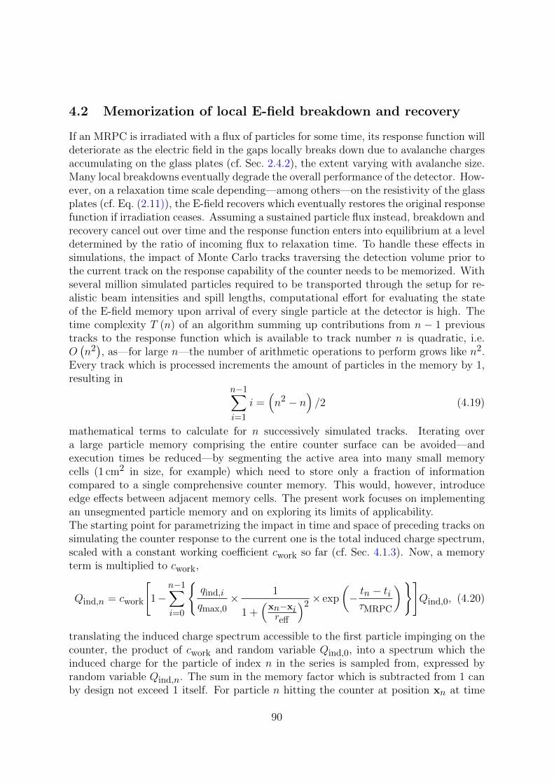
4.2 Memorization of local E-field breakdown and recovery

If an MRPC is irradiated with a flux of particles for some time, its response function willdeteriorate as the electric field in the gaps locally breaks down due to avalanche chargesaccumulating on the glass plates (cf. Sec. 2.4.2), the extent varying with avalanche size.Many local breakdowns eventually degrade the overall performance of the detector. How-ever, on a relaxation time scale depending—among others—on the resistivity of the glassplates (cf. Eq. (2.11)), the E-field recovers which eventually restores the original responsefunction if irradiation ceases. Assuming a sustained particle flux instead, breakdown andrecovery cancel out over time and the response function enters into equilibrium at a leveldetermined by the ratio of incoming flux to relaxation time. To handle these effects insimulations, the impact of Monte Carlo tracks traversing the detection volume prior tothe current track on the response capability of the counter needs to be memorized. Withseveral million simulated particles required to be transported through the setup for re-alistic beam intensities and spill lengths, computational effort for evaluating the stateof the E-field memory upon arrival of every single particle at the detector is high. Thetime complexity T (n) of an algorithm summing up contributions from n − 1 previoustracks to the response function which is available to track number n is quadratic, i.e.O(n2), as—for large n—the number of arithmetic operations to perform grows like n2.

Every track which is processed increments the amount of particles in the memory by 1,resulting in

n−1∑i=1

i =(n2 − n

)/2 (4.19)

mathematical terms to calculate for n successively simulated tracks. Iterating overa large particle memory comprising the entire counter surface can be avoided—andexecution times be reduced—by segmenting the active area into many small memorycells (1 cm2 in size, for example) which need to store only a fraction of informationcompared to a single comprehensive counter memory. This would, however, introduceedge effects between adjacent memory cells. The present work focuses on implementingan unsegmented particle memory and on exploring its limits of applicability.The starting point for parametrizing the impact in time and space of preceding tracks onsimulating the counter response to the current one is the total induced charge spectrum,scaled with a constant working coefficient cwork so far (cf. Sec. 4.1.3). Now, a memoryterm is multiplied to cwork,

Qind,n = cwork

[1−

n−1∑i=0

qind,i

qmax,0× 1

1 +(xn−xireff

)2× exp

(− tn − tiτMRPC

)]Qind,0, (4.20)

translating the induced charge spectrum accessible to the first particle impinging on thecounter, the product of cwork and random variable Qind,0, into a spectrum which theinduced charge for the particle of index n in the series is sampled from, expressed byrandom variable Qind,n. The sum in the memory factor which is subtracted from 1 canby design not exceed 1 itself. For particle n hitting the counter at position xn at time

90

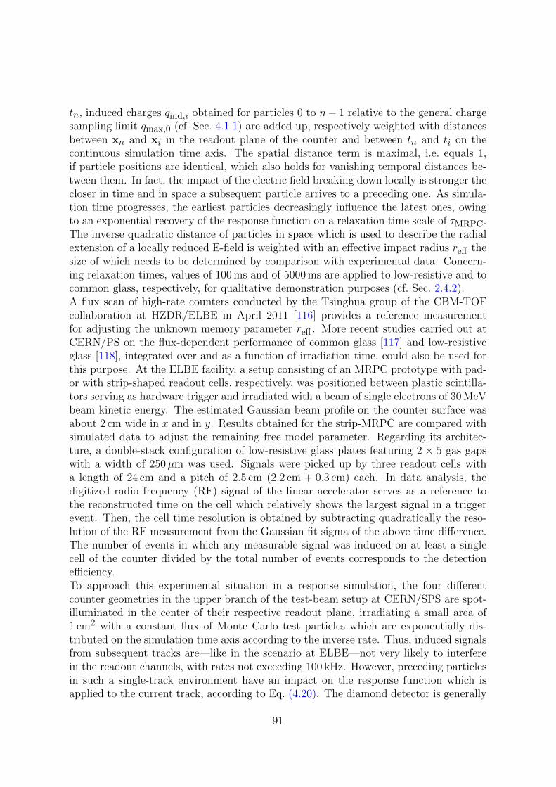
tn, induced charges qind,i obtained for particles 0 to n− 1 relative to the general chargesampling limit qmax,0 (cf. Sec. 4.1.1) are added up, respectively weighted with distancesbetween xn and xi in the readout plane of the counter and between tn and ti on thecontinuous simulation time axis. The spatial distance term is maximal, i.e. equals 1,if particle positions are identical, which also holds for vanishing temporal distances be-tween them. In fact, the impact of the electric field breaking down locally is stronger thecloser in time and in space a subsequent particle arrives to a preceding one. As simula-tion time progresses, the earliest particles decreasingly influence the latest ones, owingto an exponential recovery of the response function on a relaxation time scale of τMRPC.The inverse quadratic distance of particles in space which is used to describe the radialextension of a locally reduced E-field is weighted with an effective impact radius reff thesize of which needs to be determined by comparison with experimental data. Concern-ing relaxation times, values of 100 ms and of 5000 ms are applied to low-resistive and tocommon glass, respectively, for qualitative demonstration purposes (cf. Sec. 2.4.2).A flux scan of high-rate counters conducted by the Tsinghua group of the CBM-TOFcollaboration at HZDR/ELBE in April 2011 [116] provides a reference measurementfor adjusting the unknown memory parameter reff . More recent studies carried out atCERN/PS on the flux-dependent performance of common glass [117] and low-resistiveglass [118], integrated over and as a function of irradiation time, could also be used forthis purpose. At the ELBE facility, a setup consisting of an MRPC prototype with pad-or with strip-shaped readout cells, respectively, was positioned between plastic scintilla-tors serving as hardware trigger and irradiated with a beam of single electrons of 30 MeVbeam kinetic energy. The estimated Gaussian beam profile on the counter surface wasabout 2 cm wide in x and in y. Results obtained for the strip-MRPC are compared withsimulated data to adjust the remaining free model parameter. Regarding its architec-ture, a double-stack configuration of low-resistive glass plates featuring 2 × 5 gas gapswith a width of 250µm was used. Signals were picked up by three readout cells witha length of 24 cm and a pitch of 2.5 cm (2.2 cm + 0.3 cm) each. In data analysis, thedigitized radio frequency (RF) signal of the linear accelerator serves as a reference tothe reconstructed time on the cell which relatively shows the largest signal in a triggerevent. Then, the cell time resolution is obtained by subtracting quadratically the reso-lution of the RF measurement from the Gaussian fit sigma of the above time difference.The number of events in which any measurable signal was induced on at least a singlecell of the counter divided by the total number of events corresponds to the detectionefficiency.To approach this experimental situation in a response simulation, the four differentcounter geometries in the upper branch of the test-beam setup at CERN/SPS are spot-illuminated in the center of their respective readout plane, irradiating a small area of1 cm2 with a constant flux of Monte Carlo test particles which are exponentially dis-tributed on the simulation time axis according to the inverse rate. Thus, induced signalsfrom subsequent tracks are—like in the scenario at ELBE—not very likely to interferein the readout channels, with rates not exceeding 100 kHz. However, preceding particlesin such a single-track environment have an impact on the response function which isapplied to the current track, according to Eq. (4.20). The diamond detector is generally

91

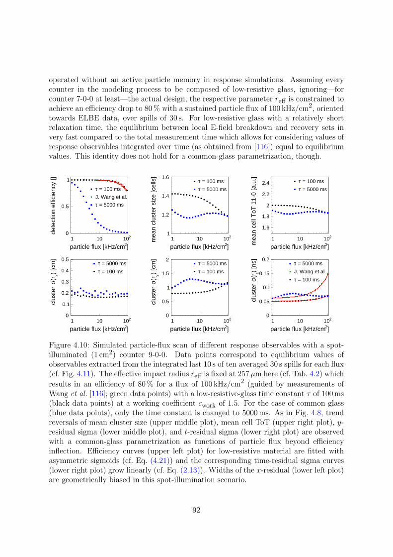
operated without an active particle memory in response simulations. Assuming everycounter in the modeling process to be composed of low-resistive glass, ignoring—forcounter 7-0-0 at least—the actual design, the respective parameter reff is constrained toachieve an efficiency drop to 80 % with a sustained particle flux of 100 kHz/cm2, orientedtowards ELBE data, over spills of 30 s. For low-resistive glass with a relatively shortrelaxation time, the equilibrium between local E-field breakdown and recovery sets invery fast compared to the total measurement time which allows for considering values ofresponse observables integrated over time (as obtained from [116]) equal to equilibriumvalues. This identity does not hold for a common-glass parametrization, though.

1 10 210

]2 particle flux [kHz/cm

0

0.5

1

det

ectio

n ef

ficie

ncy

[]

= 100 msτJ. Wang et al.

= 5000 msτ

1 10 210

]2 particle flux [kHz/cm

1

1.2

1.4

1.6

mea

n cl

uste

r si

ze [c

ells

]

= 100 msτ = 5000 msτ

1 10 210

]2 particle flux [kHz/cm

1.6

1.8

2

2.2

2.4

mea

n ce

ll T

oT 1

1-0

[a.u

.] = 100 msτ = 5000 msτ

1 10 210

]2 particle flux [kHz/cm

0

0.1

0.2

0.3

0.4

0.5

) [c

m]

x(rσ

clu

ster

= 5000 msτ = 100 msτ

1 10 210

]2 particle flux [kHz/cm

0

0.5

1

1.5

2

) [c

m]

y(rσ

clu

ster

= 5000 msτ = 100 msτ

1 10 210

]2 particle flux [kHz/cm

0

0.05

0.1

0.15

0.2)

[ns]

t(rσ

clu

ster

= 5000 msτJ. Wang et al.

= 100 msτ

Figure 4.10: Simulated particle-flux scan of different response observables with a spot-illuminated (1 cm2) counter 9-0-0. Data points correspond to equilibrium values ofobservables extracted from the integrated last 10 s of ten averaged 30 s spills for each flux(cf. Fig. 4.11). The effective impact radius reff is fixed at 257µm here (cf. Tab. 4.2) which

results in an efficiency of 80 % for a flux of 100 kHz/cm2 (guided by measurements ofWang et al. [116]; green data points) with a low-resistive-glass time constant τ of 100 ms(black data points) at a working coefficient cwork of 1.5. For the case of common glass(blue data points), only the time constant is changed to 5000 ms. As in Fig. 4.8, trendreversals of mean cluster size (upper middle plot), mean cell ToT (upper right plot), y-residual sigma (lower middle plot), and t-residual sigma (lower right plot) are observedwith a common-glass parametrization as functions of particle flux beyond efficiencyinflection. Efficiency curves (upper left plot) for low-resistive material are fitted withasymmetric sigmoids (cf. Eq. (4.21)) and the corresponding time-residual sigma curves(lower right plot) grow linearly (cf. Eq. (2.13)). Widths of the x-residual (lower left plot)are geometrically biased in this spot-illumination scenario.

92

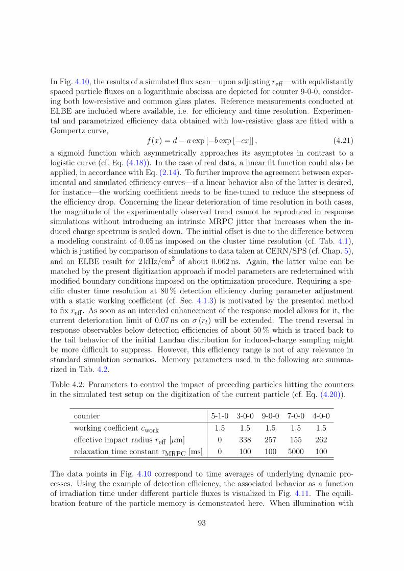
In Fig. 4.10, the results of a simulated flux scan—upon adjusting reff—with equidistantlyspaced particle fluxes on a logarithmic abscissa are depicted for counter 9-0-0, consider-ing both low-resistive and common glass plates. Reference measurements conducted atELBE are included where available, i.e. for efficiency and time resolution. Experimen-tal and parametrized efficiency data obtained with low-resistive glass are fitted with aGompertz curve,

f(x) = d− a exp [−b exp [−cx]] , (4.21)

a sigmoid function which asymmetrically approaches its asymptotes in contrast to alogistic curve (cf. Eq. (4.18)). In the case of real data, a linear fit function could also beapplied, in accordance with Eq. (2.14). To further improve the agreement between exper-imental and simulated efficiency curves—if a linear behavior also of the latter is desired,for instance—the working coefficient needs to be fine-tuned to reduce the steepness ofthe efficiency drop. Concerning the linear deterioration of time resolution in both cases,the magnitude of the experimentally observed trend cannot be reproduced in responsesimulations without introducing an intrinsic MRPC jitter that increases when the in-duced charge spectrum is scaled down. The initial offset is due to the difference betweena modeling constraint of 0.05 ns imposed on the cluster time resolution (cf. Tab. 4.1),which is justified by comparison of simulations to data taken at CERN/SPS (cf. Chap. 5),

and an ELBE result for 2 kHz/cm2 of about 0.062 ns. Again, the latter value can bematched by the present digitization approach if model parameters are redetermined withmodified boundary conditions imposed on the optimization procedure. Requiring a spe-cific cluster time resolution at 80 % detection efficiency during parameter adjustmentwith a static working coefficient (cf. Sec. 4.1.3) is motivated by the presented methodto fix reff . As soon as an intended enhancement of the response model allows for it, thecurrent deterioration limit of 0.07 ns on σ (rt) will be extended. The trend reversal inresponse observables below detection efficiencies of about 50 % which is traced back tothe tail behavior of the initial Landau distribution for induced-charge sampling mightbe more difficult to suppress. However, this efficiency range is not of any relevance instandard simulation scenarios. Memory parameters used in the following are summa-rized in Tab. 4.2.

Table 4.2: Parameters to control the impact of preceding particles hitting the countersin the simulated test setup on the digitization of the current particle (cf. Eq. (4.20)).

counter 5-1-0 3-0-0 9-0-0 7-0-0 4-0-0

working coefficient cwork 1.5 1.5 1.5 1.5 1.5

effective impact radius reff [µm] 0 338 257 155 262

relaxation time constant τMRPC [ms] 0 100 100 5000 100

The data points in Fig. 4.10 correspond to time averages of underlying dynamic pro-cesses. Using the example of detection efficiency, the associated behavior as a functionof irradiation time under different particle fluxes is visualized in Fig. 4.11. The equili-bration feature of the particle memory is demonstrated here. When illumination with

93

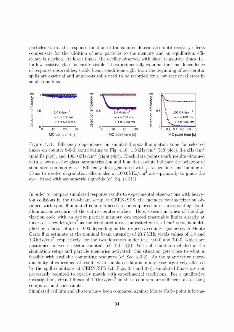
particles starts, the response function of the counter deteriorates until recovery effectscompensate for the addition of new particles to the memory and an equilibrium effi-ciency is reached. At lower fluxes, the decline observed with short relaxation times, i.e.for low-resistive glass, is hardly visible. To experimentally examine the time dependenceof response observables, stable beam conditions right from the beginning of acceleratorspills are essential and numerous spills need to be recorded for a low statistical error insmall time bins.

0 10 20 30

MC point time [s]

0

0.5

1

det

ectio

n ef

ficie

ncy

[]

21.0 kHz/cm

= 100 msτ = 5000 msτ

0 10 20 30

MC point time [s]

0

0.5

1 d

etec

tion

effic

ienc

y []

23.4 kHz/cm

= 100 msτ = 5000 msτ

0 0.2 0.4 0.6 0.8 1

MC point time [s]

0

0.5

1

det

ectio

n ef

ficie

ncy

[]

2100.0 kHz/cm

= 100 msτ = 5000 msτ

Figure 4.11: Efficiency dependence on simulated spot-illumination time for selectedfluxes on counter 9-0-0, contributing to Fig. 4.10: 1.0 kHz/cm2 (left plot), 3.4 kHz/cm2

(middle plot), and 100.0 kHz/cm2 (right plot). Black data points mark results obtainedwith a low-resistive glass parametrization and blue data points indicate the behavior ofsimulated common glass. Efficiency data generated with a rather fine time binning of50 ms to resolve degradation effects also at 100.0 kHz/cm2 are—primarily to guide theeye—fitted with asymmetric sigmoids (cf. Eq. (4.21)).

In order to compare simulated response results to experimental observations with heavy-ion collisions in the test-beam setup at CERN/SPS, the memory parametrization ob-tained with spot-illuminated counters needs to be employed in a corresponding flood-illumination scenario of the entire counter surface. Here, execution times of the digi-tization code with an active particle memory can exceed reasonable limits already atfluxes of a few kHz/cm2 as the irradiated area, contrasted with a 1 cm2 spot, is multi-plied by a factor of up to 1000 depending on the respective counter geometry. A MonteCarlo flux estimate at the nominal beam intensity of 23.7 MHz yields values of 1.5 and1.3 kHz/cm2, respectively, for the two detectors under test, 9-0-0 and 7-0-0, which arepositioned between selector counters (cf. Tab. 3.3). With all counters included in thesimulation setup and particle memories activated, this situation gets close to what isfeasible with available computing resources (cf. Sec. 4.3.2). As the quantitative repro-ducibility of experimental results with simulated data is in any case negatively affectedby the spill conditions at CERN/SPS (cf. Figs. 3.5 and 3.6), simulated fluxes are notnecessarily required to exactly match with experimental conditions. For a qualitativeinvestigation, virtual fluxes of 1.0 kHz/cm2 on these counters are sufficient, also easingcomputational constraints.Simulated cell hits and clusters have been compared against Monte Carlo point informa-

94

tion so far, unambiguously associating a response cluster with a single generating MCtrack. Concerning multiple heavy-ion collision secondaries impinging on the counter sur-face within a short time window, signal interference effects remove this clear assignmentby merging several tracks into a single cluster with possibly distorted coordinates intime and space. To have a clean, i.e. practically interference-free reference scenario forflood-illuminated counters at hand which provides direct comparability to Monte Carlo,counters 9-0-0 and 7-0-0 are—in separate runs—homogeneously irradiated with singlemuon tracks at 3 GeV/c momentum originating from the target volume, for a sustainedperiod of 10 s to mimic the spill length at CERN/SPS. Response observables as a func-tion of MC point time in spill are plotted in Fig. 4.12.

0 2 4 6 8 10

MC point time [s]

0

0.5

1

det

ectio

n ef

ficie

ncy

[]

= 100 ms)τ9-0-0 (

= 5000 ms)τ7-0-0 (

0 2 4 6 8 10

MC point time [s]

1

1.2

1.4

1.6

mea

n cl

uste

r si

ze [c

ells

]

= 100 ms)τ9-0-0 (

= 5000 ms)τ7-0-0 (

0 2 4 6 8 10

MC point time [s]

1.6

1.8

2

2.2

2.4

mea

n ce

ll T

oT 1

1-0

[a.u

.] = 100 ms)τ9-0-0 (

= 5000 ms)τ7-0-0 (

0 2 4 6 8 10

MC point time [s]

0

0.1

0.2

0.3

0.4

0.5

) [c

m]

x(rσ

clu

ster

= 5000 ms)τ7-0-0 (

= 100 ms)τ9-0-0 (

0 2 4 6 8 10

MC point time [s]

0

0.5

1

1.5

2

) [c

m]

y(rσ

clu

ster

= 5000 ms)τ7-0-0 (

= 100 ms)τ9-0-0 (

0 2 4 6 8 10

MC point time [s]

0

0.05

0.1

0.15

) [n

s]t

(rσ c

lust

er

= 5000 ms)τ7-0-0 (

= 100 ms)τ9-0-0 (

Figure 4.12: Dependence of efficiency (upper left plot), mean cluster size (upper middleplot), mean cell ToT (upper right plot), and cluster residual sigmas in x (lower left plot),y (lower middle plot), and t (lower right plot) on the illumination time of counters 9-0-0(equipped with low-resistive glass; black data points) and 7-0-0 (equipped with commonglass; blue data points). Detectors are exposed to a constant flux of single 3 GeV/c muons(no MC track interference in an event) impinging on the full counter area, respectively, at

1 kHz/cm2. Simulated muon tracks originate from the target volume of the CERN/SPSsetup (cf. Fig. 3.3). Time averages of the degrading common-glass performance areindicated by dashed blue lines. Ideally reconstructed clusters on the counter surfaces,taking into account all digis originating from a muon track without applying cluster-building conditions, are unambiguously matched against MC information for residualformation.

The initial offsets between mean cluster sizes and x-residual widths are due to inde-pendent outcome of parameter optimization (cf. Tab. 4.1) and to different readout-cell

95

geometries (cf. Tab. 3.1), respectively. Towards the end of a spill, the onset of equilibra-tion between breakdown and recovery of the electric field, i.e. induced charge spectrum,is visible. No trend reversals occur with the common-glass parametrization which provesthe response model to be applicable in the considered efficiency range.

4.3 Implementation in a time-based simulation framework

4.3.1 Signal interference handling

Building on general remarks concerning the simulation strategy realized in CbmRootto transform event-based input data into time-based output data given in Sec. 2.3, thepeculiarities of the digitization software developed for the TOF subsystem are describedhereinafter. Upon propagating collision secondaries event by event through the virtualsetup with a Monte Carlo transport code, the run manager—in the subsequent digi-tization stage—reads prepared events from file and samples event start times from anexponential distribution of inter-event intervals, the mean length of which corresponds tothe inverse product of beam intensity and interaction probability with the target. Timestamps of Monte Carlo points belonging to an event are augmented with the respectiveevent start time placing them on a continuous simulation time axis. All MC points in anevent which result from an intersection between a MC track and a TOF counter volume(averaging times and positions of entry into individual gas gaps during transport) aresorted by time and filled into a buffer. The digitization class implemented in this workreads time-sorted MC points from this buffer with time stamps smaller than the currentevent start time, optionally inserting MC points associated with an adjustable counterdark rate beforehand. In the first event, only a single point created in the diamonddetector is extracted from the buffer which originates from a straight-line extrapolationof the collision point in the target to the diamond volume against the beam direction,yielding a time stamp prior to the collision time by subtracting the time of flight ofbeam particles between diamond and target from the latter. In subsequent events, MCpoints from the preceding one are read out unless they are positioned in time later thanthe current event start time which splits events for digitization and can lead to eventmixing.For every MC point which is passed to the digitization algorithm, the counter response iscalculated according to Secs. 4.1 and 4.2 which comprises adding—if enabled—the corre-sponding tuple of induced charge qind,i, spatial coordinates xi, and time ti to the particlememory of the respective counter. If induced signals exceed discrimination threshold,transient digi objects are constructed—yet without digitization (TDC) jitter—and filledinto a signal buffer which is in charge of interference handling. The output format ofdetector raw messages comprising a (leading-edge) time stamp and a ToT value is usedfor this purpose as signal interference—in the present implementation—depends on therelative positioning of leading and trailing edges (time stamp plus ToT) of subsequentsignals in time only. In an iterative merging procedure, the current digi is successivelychecked for overlapping ToT ranges with digis from the same readout channel which

96

reside in the buffer. Upon a positive interference evaluation, the original pair of digis iscombined into a new digi carrying the earliest leading-edge time stamp and the latesttrailing-edge time stamp of the two parent digis which are deleted afterwards. As theresulting digi, in turn, might overlap with other digis in the buffer (in case of a newlyarriving digi bridging the ToT gap between two detached buffered digis, for instance), in-terference handling continues until the buffer exclusively contains non-overlapping digisfor the respective readout channel.After treating all MC points eligible for digitization in the current round of method callsby the framework in the described manner, digi objects with a ToT interval ending priorto the current event start time are removed from the signal buffer for further processing.Detector signals generated by a MC point which is positioned on the continuous axisright after the current readout time of the signal buffer are assumed not to interferewith extracted digis anymore. This assumption is based on identical propagation timesof subsequent signals in the same readout channel with a fixed time offset of 14 ns appliedto the Landau parametrization (cf. Eq. (4.3)), ensuring a safe distance between MonteCarlo point times and leading-edge time stamps of corresponding digis. Under thesepremises, it is unlikely that a digi—due to electronics jitter and/or time walk—is posi-tioned in time prior to the generating MC point, considering also the finite propagationtime of signals along the cell if induction does not occur right at longitudinal cell ends.The opposite case would allow for the leading edge of a subsequent signal to precede thetrailing edge of a signal already removed from the buffer, erroneously supposing thatfurther interference handling was not necessary.Upon extraction from the signal buffer, both leading- and trailing-edge time stampsof non-interfering digis are compared with the corresponding memorized values of thepreceding digi in the respective readout channel. If the time difference in either caseis larger than an adjustable TDC dead time, the digi object is preserved, otherwisedropped. Then, digitization jitter is added to both edge measurements. A summarysketch of interference handling for simulated counters is provided in Fig. 4.13.Optionally, the calibration obtained with cell hits during response modeling can be ap-plied at this stage, including the scaling of ToT spectra and time-offset and time-walkcorrections (cf. Sec. 4.1.1). By the merging of digis overlapping in ToT, a bias is in-troduced onto the relation between leading-edge time and time over threshold. A smallsignal with an originally short ToT that is combined with a subsequent signal receivesa larger new ToT value which is associated with a signal amplitude bigger than theoriginal one. Consequently, performing a time-walk correction based on merged ToTranges would yield wrong compensation values for the amplitude-dependent variation ofthreshold crossing times. Hence, the digitization class keeps track of the original assign-ment between signal time stamp and ToT to properly account for the time-walk effect.Throughout this work, simulated digis are calibrated with this method. A potential usecase for non-ideal detector data obtained from simulations could be testing the calibra-tion chain for real data (cf. Sec. 3.3).Finally processed MRPC digis are moved to an output buffer for timeslice building whichis common to all simulated CBM subsystems. To make sure that a timeslice of variablesize, e.g. the mean distance between events multiplied by one thousand, is not closed

97

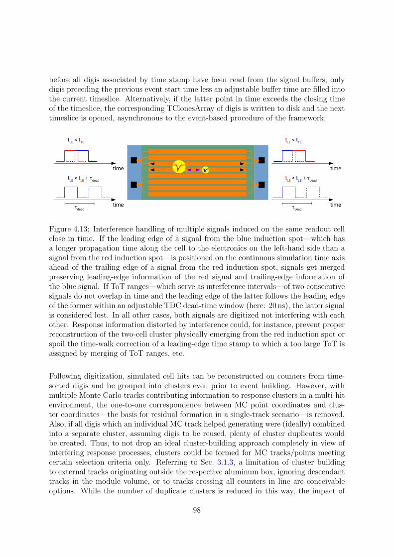
before all digis associated by time stamp have been read from the signal buffers, onlydigis preceding the previous event start time less an adjustable buffer time are filled intothe current timeslice. Alternatively, if the latter point in time exceeds the closing timeof the timeslice, the corresponding TClonesArray of digis is written to disk and the nexttimeslice is opened, asynchronous to the event-based procedure of the framework.

time

time

tLE < tTE

tLE < tLE + tdead

tdead

time

time

tLE < tTE

tLE < tLE + tdead

tdead

Figure 4.13: Interference handling of multiple signals induced on the same readout cellclose in time. If the leading edge of a signal from the blue induction spot—which hasa longer propagation time along the cell to the electronics on the left-hand side than asignal from the red induction spot—is positioned on the continuous simulation time axisahead of the trailing edge of a signal from the red induction spot, signals get mergedpreserving leading-edge information of the red signal and trailing-edge information ofthe blue signal. If ToT ranges—which serve as interference intervals—of two consecutivesignals do not overlap in time and the leading edge of the latter follows the leading edgeof the former within an adjustable TDC dead-time window (here: 20 ns), the latter signalis considered lost. In all other cases, both signals are digitized not interfering with eachother. Response information distorted by interference could, for instance, prevent properreconstruction of the two-cell cluster physically emerging from the red induction spot orspoil the time-walk correction of a leading-edge time stamp to which a too large ToT isassigned by merging of ToT ranges, etc.

Following digitization, simulated cell hits can be reconstructed on counters from time-sorted digis and be grouped into clusters even prior to event building. However, withmultiple Monte Carlo tracks contributing information to response clusters in a multi-hitenvironment, the one-to-one correspondence between MC point coordinates and clus-ter coordinates—the basis for residual formation in a single-track scenario—is removed.Also, if all digis which an individual MC track helped generating were (ideally) combinedinto a separate cluster, assuming digis to be reused, plenty of cluster duplicates wouldbe created. Thus, to not drop an ideal cluster-building approach completely in view ofinterfering response processes, clusters could be formed for MC tracks/points meetingcertain selection criteria only. Referring to Sec. 3.1.3, a limitation of cluster buildingto external tracks originating outside the respective aluminum box, ignoring descendanttracks in the module volume, or to tracks crossing all counters in line are conceivableoptions. While the number of duplicate clusters is reduced in this way, the impact of

98

signal interference, a response feature in a multi-track situation, is not.In Fig. 4.14, cluster residuals in x, y, and t between external MC points and the associ-ated ideal collections of digis are depicted which exhibit interference effects. Concerningthe ToT-weighted centers of cluster cells from which the x-position across the readoutplane is derived, merged ToT ranges of interfering signals affect the weighting method,in particular for larger clusters. If a double hit is registered on a cell within a short timewindow (cf. Fig. 4.13), timing information—assuming signals on opposing cell ends tooverlap in ToT—is preserved only on one side of the readout cell, respectively, one digireflecting the arrival time of the first hit and the other digi referring to the passage ofthe second hit through the counter. Neither in time nor in y-position a reconstruction ofactual single hit coordinates is possible in this situation. Due to allegedly shorter signalpropagation times along the cell, losing information on the interval between inductionpoints, a hit time is calculated by averaging top and bottom time stamps which precedesthe MC point times of the two original tracks. The y-position along the readout planeis determined from propagation-time differences of the induced signal to opposing endsof the cell. Signal propagation times are similar for a hit in the longitudinal center ofthe cell and differ most if induction occurs close to a cell end. Considering interferingsignals from two opposing peripheral hits, the time differences that would be obtainedin separate processing balance out here, positioning the reconstructed hit in the cellcenter. For a central and a peripheral hit on the same cell, either originally similar prop-agation times become more unequal or initially asymmetric propagation times becomemore equal, depending on the respective point of view. In any case, the reconstructedhit is located between the two original ones, pulling the y-residual symmetrically apart.Special attention to response distortions caused by signal interference effects needs tobe paid in multi-hit data analysis (cf. Sec. 5.2).

Std Dev 0.232Sigma 0.2061

4− 2− 0 2 4

[cm]x cluster r

1

10

210

310

410

510

610Std Dev 0.232Sigma 0.2061

Std Dev 2.17Sigma 0.8263

10− 0 10

[cm]y cluster r

310

410

510

Std Dev 2.17Sigma 0.8263

Std Dev 0.1474Sigma 0.05291

1− 0 1

[ns]t cluster r

10

210

310

410

510

610 Std Dev 0.1474Sigma 0.05291

Figure 4.14: Interference effects on cluster residuals of counter 9-0-0 seen when irra-diating the CERN/SPS setup with heavy-ion reaction secondaries, creating a multi-track environment. Residuals in x (left plot), y (middle plot), and t (right plot) areformed between ideally reconstructed clusters on the counter surface and contribut-ing MC tracks. Distortions contrasting with Fig. 4.6 originate from signal merging assketched in Fig. 4.13.

99

4.3.2 Multithreading and parallelization

An important aspect of digitization code design is the efficient implementation of anunsegmented particle memory (cf. Sec. 4.2) which stores information about the chargeinduced in the readout plane of a counter in time and in space by every single MonteCarlo point created in its detection volume in the course of a simulation. Given thequadratic time complexity of repeatedly summing up contributions from previous tracksto the response function of the current track (cf. Eq. (4.20)), a multithreaded computingstrategy is embarked on. Concretely, the summation load is shared between n parallelthreads, utilizing TThread functionality in ROOT, each handling only the nth fractionof particles in the memory. Eventually, the n partial sums are combined into the totalmemory coefficient of the induced charge spectrum available to the latest particle. Asuitable computing infrastructure to execute intrinsically parallel programs on is pro-vided by the Kronos cluster installed in the Green IT Cube at GSI (cf. Sec. 2.2). Jobscheduling for different users on a total of 530 single computing nodes forming the mainpartition of the cluster which are equipped with dual-socket motherboards is carriedout by the Slurm workload manager. Each node contains two identical CPUs from theIntel Xeon family, either a pair of E5-2660 v3 processors individually featuring 10 phys-ical cores and 20 logical threads or two E5-2680 v4 units with 14 cores and 28 threadseach. Altogether, the batch computing farm comprises 190 nodes with the former and340 nodes with the latter configuration, yielding 1,060 CPUs, 13,320 cores, and 26,640threads to be shared among users.

0 20 40 60

memory threads []

0

20

40

60

80

100310×

rea

l tim

e [s

]

particles62x10

particles61x10

0 20 40 60

memory threads []

0

20

40

60

80

100310×

CP

U ti

me

[s]

particles62x10

particles61x10

0 20 40 60

memory threads []

0

5

10

15

20

CP

U-t

o-re

al-t

ime

ratio

[]

f(x) = x

particles62x10

particles61x10

Figure 4.15: Run-time benefits of computing contributions to a particle memory com-prising one (blue data points) and two (black data points) million maximum entries bymultiple threads in parallel. Real execution times (left plot) of corresponding flood illu-minations of a counter surface with the respective amount of test particles as a functionof memory threads spawned. Total CPU time consumed by all participating threads(middle plot) indicating an increased administrative effort the more threads participatein the computation. The CPU-to-real-time ratio (right plot) visualizes the degree towhich multithreading functionality is exploited by the two benchmark simulations. Forsimulating a large amount of particles, it proves beneficial to spread the computationalload to many threads. Benchmark results shown in this figure were obtained mainlywith Intel Xeon E5-2680 v4 CPUs (14 cores, 28 threads) on dual-socket motherboards.

100

Results of a feasibility study for a multithreaded particle memory conducted on eitherone or both CPUs of a node on Kronos are presented in Fig. 4.15, for two sets of1,000,000 and 2,000,000 subsequently memorized particles that can be processed withina day of run time even by a single memory thread. Ideally, doubling the number ofdeployed threads would half job execution times as, when computing the memory coef-ficient for the current track, only half the amount of terms need to be summed up inseries. Theoretically also, twice the number of particles to simulate would correspond toan increase in execution time by a factor of four, independent from the respective threadcount, due to a quadratic time complexity of the summation algorithm. In reality, theseexpectations are not fully met. The performance gain from distributing the computa-tional load to multiple threads is diminished, especially for smaller particle numbers, bywait conditions individual threads have to obey for reasons of thread safety. With moretracks participating in the simulation, the latter effect is increasingly outweighed by thebenefit of less terms to add up in partial summation. Regarding the benchmark data inFig. 4.15, while the CPU time—indicating a quadratic growth in computational effortbetween the two samples—only slightly rises as a function of deployed memory threads,the respective real execution time drops rapidly resulting in a CPU-to-real-time ratiowhich grows linearly, in the beginning at least. Eventually, curves level off due to anincreasing computational inefficiency caused by managing more and more threads fora constant number of memory particles. The ratio between CPU and real time riseswith sample size for a given thread count which implies an improved utilization of mul-tithreading resources.To simulate the test-beam conditions at CERN/SPS, more than 10 million (externaland internal) tracks passing through a large-area prototype need to be memorized if a

particle flux of 1 kHz/cm2 on the counter surface is to be sustained over a 10 s spill.Thus, regarding Fig. 4.15 and the constraint to share computing capacities at GSI withother users, a particle memory with 39 threads (plus a main thread) is used for theproduction of simulated data on the Kronos cluster, to allow for executing jobs on bothtypes of computing nodes. Empirical run-time values measured under these premisessuggest a maximum memory size of about 30 million particles for a simulation time ofone week—without any buffer—which is the current upper limit on Kronos. Consider-ing the illumination of a single counter, not distinguishing between external rate andinternal response tracks (cf. Sec. 3.1.3), the resulting limitations on irradiation time, i.e.spill length, are given in Tab. 4.3, depending on the respective area.Prototypical counter designs MRPC1 and MRPC2 (cf. Sec. 2.4.3), to pick an example,

can be exposed to nominal particle fluxes of up to 25 kHz/cm2 for less than 5 s in simula-tions if the particle memory is enabled. Apart from the practical impossibility to reservethe entire Kronos cluster for TOF simulations, the available number of 530 computingnodes, provided that all counters could be processed in parallel on individual machines,would not suffice to cover the entire wall which is composed of 1376 MRPC1–4 counters.Thus, the applicability of the full response model developed in this work including thememory feature is limited to smaller setups like the one at CERN/SPS or mCBM atGSI/SIS18 (cf. Sec. 5.4) and to modest particle fluxes on counters if longer accelerator

101

Table 4.3: Maximum achievable particle fluxes sustained over spills of various lengths ondifferent counter geometries with an active particle memory constrained by a run-timelimit of 7 days on the Kronos computing cluster at GSI which allows for memorizing upto 30 million particles if 39 memory threads are spawned.

irradiation time/ 1 s 2 s 5 s 10 s unit

illuminated area

spot (1 cm2) 30 15 6 3 MHz/cm2

4-0-0 (60 cm2) 500 250 100 50 kHz/cm2

MRPC1 (302 cm2) 100 50 20 10 kHz/cm2

MRPC2 (604 cm2) 50 25 10 5 kHz/cm2

9-0-0 (668 cm2) 45 22.5 9 4.5 kHz/cm2

MRPC3a/b (864 cm2) 35 17.5 7 3.5 kHz/cm2

MRPC4 (1696 cm2) 18 9 3.6 1.8 kHz/cm2

spills are requested.In Fig. 4.16, the parallelized simulation workflow from Monte Carlo transport to dataanalysis is summarized, pointing also at room for improvement regarding the currentlysequential processing of counters in the digitization stage. Compared with the valuesstated in Tab. 4.3, simulating n identical counters in a row reduces the respective maxi-mum particle flux by about a factor of

√n. Multiple accelerator spills can be simulated

in parallel only if spill breaks in between are considered long enough for the detectorresponse function to fully recover in the absence of beam. This assumption is supposedto be valid for CERN/SPS data given a spill length of about 10 s followed by a 20 s breakand, hence, applied to simulations.

4.3.3 Applicability for full-featured test-beam simulations

To approach test-beam results obtained with argon-on-lead collisions in simulations,conditions at the experimental site should be reflected in software. With an estimatedbeam intensity of 23.7 MHz (cf. Sec. 3.1.2), an interaction probability between projectileand target nuclei of 4 %, and a spill duration of 10 s, about 9.5 million UrQMD collisionseeds need to be propagated through the virtual setup in a single spill to generate sus-tained external particle fluxes ranging—in mean—from 1.8 to 1.1 kHz/cm2 on the line ofcounters. The estimated digitization time (memory enabled) on the Kronos cluster forsuch a spill of beam particles leaving traces in the diamond detector and—by collisionsecondaries—in four differently sized MRPCs would amount to about 5 days which isfeasible, in principle, but gets close to the general limit of 7 days if some safety mar-gin for run-time variations between parallel jobs is included. As the spill structure atCERN/SPS is not uniform and shows a significant intensity spike in the beginning, a

102

single-threaded ROOT process

...

Monte Carlo transport

digitization

reconstruction & analysis

...

...

parallel spill processing

...

parallel counter processing

spill 0 spill N - 1 spill 0

...

multithreaded ROOT processprocess dependencies

Figure 4.16: Options for parallelizing time-based MRPC simulations with a particlememory enabled during digitization. If the particle memory is supposed to be clearedbetween spills, multiple spills can be processed in parallel as no information needs to beexchanged between different processes. For a single spill (left part), a certain amountof Monte Carlo collision seeds—depending on the desired beam intensity and beam-target interaction probability—needs to be transported through the virtual setup eventby event which happens in parallel processes (yellow boxes) which are internally single-(but potentially multi-)threaded. Digitization (green box) can start when Monte Carlotransport is finished. Intersections of tracks from transported input events with anactive detector volume (MC points) are arranged on a continuous time axis and the cor-responding induced charge is stored in the particle memory along with time and positioncoordinates. The joint impact of preceding tracks in memory on the digitization of thecurrent one is computed in parallel by multiple threads in the single digitization process,counter by counter. As a counter operates as an independent entity concerning particlememorization, execution times for digitization could be further reduced by processingmemory-active counters in parallel, not sequentially, i.e. by running a separate digitiza-tion process for every counter (right part; green boxes). This functionality is currentlynot implemented. Reconstruction and analysis following digitization—here depicted asa single-threaded synopsis (yellow box)—could be parallelized as well.

103

qualitative comprehension of trends observed in experimental data is primarily aimed atby simulating collisions in the test-beam setup rather than an exact quantitative descrip-tion of effects, following an argument already given in Sec. 4.2. Hence, a reduced beamintensity of 17.6 MHz (decreasing the demand for collision seeds to 7 million per spill)

is applied which generates a mean external particle flux of precisely 1.0 kHz/cm2 on thecommon-glass counter under test (7-0-0) and, accordingly, average fluxes of 1.348, 1.125,

and 0.830 kHz/cm2 on counters 3-0-0, 9-0-0, and 4-0-0. At the end of a digitization run,i.e. a single processed spill, with an extrapolated computing time of 2 days and 20 hourson the Kronos cluster which is a more relaxed situation, particle memories comprise—inthe sequence of counters—about 13.6, 8.8, 9.9, and 0.6 million entries under these con-ditions.

0 50 100 150 200 250 300

simulation time [s]

0

2

4

6

8

610×

dig

is /

s []

0 50 100 150 200 250 300

simulation time [s]

410

510

610

710

dig

is /

s []

Figure 4.17: Rate effects visible in production time stamps of detector digis distributedover 10 consecutive spills of simulated heavy-ion reactions (upper plot; linear scale). A10 s spill is always followed by a 20 s spill break—mimicking the spill length and dutycycle at CERN/SPS—which contains digis attributed to detector noise on the MRPCs

of 1 Hz/cm2 (lower plot; logarithmic scale). At the beginning of a new spill, the particlememory is reset.

Actual digitization times for 10 spills of this type (cf. Fig. 4.17) are listed in Tab. 4.4,comparing computational effort for otherwise identical runs with and without an activeparticle memory. Execution times systematically vary between different processors butnot for this reason alone. With the memory feature disabled, the digitization class canbe inserted into the common simulation chain of the CBM experiment.Following time-based digitization, detector raw messages (digis) reside in timeslices withinformation on the original event assignment and contributing MC points preserved in

104

Table 4.4: Digitization times (ddd-hh:mm:ss) of ten parallel spills of simulated heavy-ioncollisions (cf. Fig. 4.17), with an active (left-hand side) and an inactive (right-hand side)particle memory, executed on members of the Intel Xeon processor family on the Kronoscomputing cluster at GSI. In the case of an active particle memory, the summation ofcontributions from preceding tracks to the current response function is performed by 39threads in parallel.

spill CPU time real time ratio CPU time real time ratio processor

w/ particle memory w/o particle memory

0 112-11:52:23 03-07:39:04 33.9 00:48:01 00:51:04 0.94 E5-2660 v3

1 112-16:12:24 03-07:12:40 34.1 00:47:48 00:54:21 0.88 E5-2660 v3

2 112-22:16:45 03-06:28:56 34.5 00:47:36 00:51:17 0.93 E5-2660 v3

3 88-01:38:48 02-18:12:53 31.9 00:47:34 01:23:35 0.57 E5-2680 v4

4 87-11:08:55 02-18:08:16 31.7 00:42:47 00:46:02 0.93 E5-2680 v4

5 88-03:13:59 02-18:45:43 31.7 00:45:17 00:48:48 0.93 E5-2680 v4

6 87-17:22:18 02-19:30:21 31.2 00:45:02 00:48:19 0.93 E5-2680 v4

7 87-15:45:50 02-17:34:16 32.1 00:45:02 00:47:36 0.95 E5-2680 v4

8 88-16:00:22 03-05:17:19 27.5 00:44:18 00:47:17 0.94 E5-2680 v4

9 87-07:44:09 02-17:24:47 32.0 00:44:57 00:47:24 0.95 E5-2680 v4

dedicated backlink objects. Concerning the above heavy-ion collision simulation, a times-lice corresponds to a time interval of about 1.4 ms which contains 1000 events on average.A single spill cycle of 30 s is subdivided into 21, 120 timeslices. Prior to comparing time-based simulated to event-based experimental data in the analysis (cf. Chap. 5), eventsneed to be recovered from timeslices, either by identifying accumulations of digis on thecontinuous time axis (cf. Fig. 3.11) or—in an ideal way restricted to simulated data—byrecombining digis into events based on backlink information.For event building in the latter case, an optional branch of time-sorted Monte Carlopoints in the timeslice is scanned for coincident (by the original event number storedwith each point) track passages on a set of trigger counters. If for a given event numbera MC point is found on every required station, not necessarily originating from the sameparticle, the digi branch of the timeslice is looped over to collect raw messages referringto any MC point which is associated with the selected event. Then, these digis togetherwith all MC point objects belonging to the respective event and backward/forward ref-erences providing links between the two data formats are saved to disk as reconstructedevents, asynchronous to reading entire timeslices at the input stage. Restoring eventsin this ideal fashion only with MC point information contained in digi backlinks—incontrast to reading all MC points processed in digitization from a separate timeslicebranch—would not give a complete picture as, by this means, no record is kept of trackswhich did not induce a measurable signal on any readout cell. In the case of event

105

mixing, multiple digi backward references to points originating from different originalevents indicate a corresponding response interference which might affect digi properties.Timeslices are handled independently by the framework at the moment, i.e. events orpoints and related digis might be split across timeslice borders by any of the two event-building methods mentioned above. However, with a thousand events per timeslice thiseffect is statistically insignificant.Regarding the two simulation scenarios to be compared with experimental findingsat CERN/SPS—a homogeneous irradiation of counters under test with single muons(cf. Fig. 4.12) and a multi-track environment created by heavy-ion collisions—an idealevent building in the above sense is performed in both cases, using the diamond detector(5-1-0) and selector counters 3-0-0 and 4-0-0 as trigger stations. The corresponding se-lection bias on the different counter surfaces does not conflict with calibration routineshere as simulated digis are pre-calibrated during digitization, applying correction termsto leading-edge time stamps and ToT values which were generated in the process ofadjusting model parameters. Instead, considering collision simulations for a numericalexample, the number of events to be handled by the analysis class is reduced from about70.5 million in total, distributed over 10 subsequent spills, to 4.3 million relevant onesfor testing the two counters in the middle with reference hits on the peripheral selectorcounters—in favor of shorter execution times. Clustering of simulated cell hits is basedon correlations in time and space observed on adjacent readout cells, analogous to realdata (cf. Sec. 3.3).

106

CHAPTER 5

RESULTS

Two principal effects influencing the performance of MRPCs—and its evaluation—inheavy-ion-collision experiments at high beam–target interaction rates are under investi-gation in this work. On the one hand, the response function deteriorates with irradiationtime owing to a local breakdown of the electric field in the gas gaps upon avalanche for-mation. The observed decline in detection capability, reducing efficiency and wideningtime and position residuals, depends on the relation between incident particle flux andrelaxation time for field recovery, the latter quantity being constrained mainly by theresistivity of the glass plates. On the other hand, multiple signals induced on the samereadout cell by different collision secondaries may interfere with each other, mergingresponse information and distorting residuals. With increasing projectile energies andgrowing sizes of colliding nuclei, counters are noticeably exposed to such multi-hit condi-tions which complicate the matching of correlated response clusters between two MRPCsor the unambiguous assignment of a cluster to an extrapolated particle trajectory whichis reconstructed by a tracking system. The novel detector response parametrizationdescribed in Chap. 4 takes into account both rate and signal-interference effects. Thisallows for a systematic comparison of corresponding trends in the response functionmeasured during the test beam at CERN/SPS with simulated data which is the subjectof the present chapter.Due to the lack of an ideal Monte Carlo reference for experimental clusters generatedon a single counter, response observables in data analysis, concerning both simulatedand real events, need to be evaluated against a matched cluster on another counter inthe setup. The four counters are positioned in line (cf. Fig. 3.3) to obtain responsecorrelations on different detectors primarily from straight particle tracks which consec-utively pass through all stations. Cluster matching in time and space is realized witha conventional χ2-formalism on two levels. First, events comprising a sufficiently wellmatched cluster pair on selector counters 3-0-0 and 4-0-0 positioned in the very front andin the very back, respectively, are identified. Then, in these events, one of two detectorsunder test (DUT) mounted between selector counters is scanned for a cluster match-ing the interpolated coordinates of the selector hit on reference counter 4-0-0, againstwhich residuals are calculated for the best match available. Not finding a match at allor only a poor one is counted towards detection inefficiency. Response characteristicsdiffer with applied χ2-limits but also with MRPC design and irradiation scenario. Themain distinguishing feature between DUT counters 9-0-0 and 7-0-0 is the resistivity ofthe glass plates, the former being constructed with low-resistive material while the latteris equipped with common glass. In simulations, this is reflected by different relaxationtimes of τMRPC = 100 ms and τMRPC = 5000 ms, respectively. Experimental resultsfor these counters (labeled with “exp data”) are compared to findings with simulatedheavy-ion collisions (“sim data”) and single muon tracks (“sim ST”)—providing a multi-and a single-hit scenario as points of reference—in two respects: the interference bias on

107

counter response as a function of hit multiplicity and the degradation of performancedue to rate as a function of irradiation time.In Sec. 5.1, the χ2-method for cluster selection and matching is described and limitationsare discussed. Considering the cluster multiplicity on the first counter in line (3-0-0) asa measure of signal interference, multi-hit effects are studied as a function of a limit onthis observable in Sec. 5.2. The impact of a sustained particle flux on counter responsewith progressing time in spill is examined in Sec. 5.3. Finally, an outlook is given inSec. 5.4 on a continuation of the current research activity at the running mCBM exper-iment at GSI/SIS18 where rate and multi-hit conditions are even more challenging thanat CERN/SPS.

5.1 Event selection and hit matching in data analysis

The starting point for analysis of both experimental and simulated data are arrays ofcalibrated hits (clusters) on counters in the setup, each representing an input event. Ina physics production run, contrary to a test-beam scenario for detector prototypes, onewould aim at reconstructing—from correlations on different stations—and identifying,e.g. by the TOF method, all particle trajectories in an event within the geometricalacceptance of the experiment. At CERN/SPS, full-scale PID (particle identification)instrumentation as required for this purpose was not available and is also not necessaryto evaluate the mere counter performance under various aspects. The analysis strategypursued in this work concentrates on finding the best possible hit match on a detectorunder test to an optimal prediction based on correlations between hits on a pair of selec-tor counters. Thus, apart from a mandatory hit on the diamond detector, a maximum ofthree clusters—two on selectors Sel1 (4-0-0) and Sel2 (3-0-0) and one on DUT (9-0-0 or7-0-0) if existing—is considered in a sample of events which is compiled according to thematching quality among selector hits. Clusters obtained for analysis from experimentand simulations represent the earliest response occurrences on contributing readout cellsin the respective event, owing to a TDC channel dead time of (about) 20 ns and, inaddition, to an adjustable minimum distance—here of 50 ns—between consecutive digisin a readout channel applied during cluster building. Hence, multiple signals inducedby different tracks on a single cell are regarded in data analysis only insofar as they aremerged by interference.The matching algorithm is fairly straightforward and premised on assumed chi-squaredistributions of weighted cluster residuals in dimensions x, y, and t. In a given event, thecluster pair with minimum residual χ2 is identified, successively for counter combina-tions Sel2–Sel1 and DUT–Sel1 if a limit on selector χ2 is not exceeded. The first selectorcounter provides a reference measurement for the DUT which is supported by the bestmatching cluster on Sel2. Concerning global position residuals, a straight-line interpola-tion of cluster coordinates on the counter which is installed further downstream (alwaysSel1) translates this information into the readout plane of the counter which is locatedcloser to the target (either Sel2 or DUT). Due to varying readout-cell orientations acrosscounters, the cells of counter 4-0-0 running parallel to cave-y while cells on the counters

108

in front are oriented along cave-x (cf. Tab. 3.2), local x- and y-coordinates enter intoglobal x- and y-residuals for the counter in the back only. For the other counters, globaland local coordinates are swapped which is important to note as response calculationsalong and across readout cells systematically differ. Upon digi calibration, time residu-als in particular are not strictly centered about zero, neither for real data where smalldeviations can occur nor for simulated data. In the latter case, offsets corresponding tothe average time of flight between stations need to be subtracted from cluster residualmeans, as time stamps are ideally calibrated against the actual passage of a Monte Carlotrack through the detector.

Mean 0.0006255Sigma 0.8913

20− 10− 0 10 20

[cm]x Sel r

1

10

210

310

410

Mean 0.0006255Sigma 0.8913

Mean 0.006827− Sigma 0.74

20− 10− 0 10 20

[cm]y Sel r

10

210

310

410

Mean 0.006827− Sigma 0.74

Mean 0.002059Sigma 0.09101

2− 0 2

[ns]t Sel r

10

210

310

410

Mean 0.002059Sigma 0.09101

Mean 0.0009883− Sigma 0.5277

20− 10− 0 10 20

[cm]x Sel-NN r

1

10

210

310

410Mean 0.0009883− Sigma 0.5277

Mean 0.0007848− Sigma 0.5034

20− 10− 0 10 20

[cm]y Sel-NN r

1

10

210

310

410Mean 0.0007848− Sigma 0.5034

Mean 05−7.883e− Sigma 0.06509

2− 0 2

[ns]t Sel-NN r

1

10

210

310

410Mean 05−7.883e− Sigma 0.06509

Figure 5.1: Illustration of event selection for analysis based on experimental residualsbetween cluster pairs on selector counters 3-0-0 (Sel2) and 4-0-0 (Sel1) with minimalresidual χ2 (cf. Eq. (5.1)) in three global dimensions x (left column), y (middle column),and t (right column) in the respective event (upper row). Peaks of the centered residualdistributions are fitted with Gaussian functions (red curves) to obtain initial values forχ2-weight estimation (cf. Fig. 5.2). A cut on the properly weighted residual Sel χ2 (of2.5 if not otherwise stated) qualifies a subset of events (green distributions) for analysisof detectors under test (DUT). In these selected events, the nearest-neighbor (NN) DUTcluster to the Sel1 cluster which contributes to the selector pair is determined with ananalogous Sel-NN χ2-mechanism. Residuals between the χ2-matched cluster on DUTcounter 9-0-0 and the prediction from Sel1 (reference) counter 4-0-0, constrained by Sel2counter 3-0-0, are shown in the lower row. Sel-NN residuals confined by a χ2-cut (of5.0 if not otherwise stated; green distributions) are the basis for extrapolating detectionefficiency.

Centering residual distributions and determining χ2-weights for cluster matching be-

109

tween selector counters (labeled with Sel) on one side and between DUT and Sel1 (la-beled with Sel-NN for nearest neighbor) on the other side is a nested process owing tothe dependence of the latter on the χ2-limit applied to the former. Prior to imposingany cut on Sel χ2, peaks of residual distributions of selector cluster pairs with the lowestrelative χ2-value in the respective event, using default weights of w(rx) = w(ry) = 1 cmand w(rt) = 0.1 ns in the three response dimensions, are fitted with Gaussian func-tions yielding—by extracted mean and sigma values—offsets for centering and initialestimates for actual χ2-weights. Fitting ranges stated in Tab. 5.1 are limited to smallintervals about residual peaks due to the inherent background in Sel spectra withoutevent filtering (cf. Fig. 5.1). For the χ2-method to be applicable, widths of the Gaussiancore of distributions need to be considered.

Table 5.1: Ranges for Sel and Sel-NN residual peak fitting (cf. Fig. 5.1) applied to thepair of selector counters (3-0-0 and 4-0-0) and to subsequent DUT matching of counters9-0-0 and 7-0-0 in experimental data, simulated heavy-ion reaction data, and simulatedsingle-track (ST) muon data.

3-0-0 & 4-0-0 exp data sim data sim ST

Sel rx fitting range [cm] ±1.0 ±1.0 ±1.0

Sel ry fitting range [cm] ±1.0 ±1.0 ±1.0

Sel rt fitting range [ns] ±0.15 ±0.15 ±0.15

9-0-0 exp data sim data sim ST

Sel-NN rx fitting range [cm] ±1.0 ±1.2 ±1.2

Sel-NN ry fitting range [cm] ±1.0 ±1.0 ±1.0

Sel-NN rt fitting range [ns] ±0.15 ±0.15 ±0.15

7-0-0 exp data sim data sim ST

Sel-NN rx fitting range [cm] ±2.0 ±1.2 ±1.2

Sel-NN ry fitting range [cm] ±1.3 ±1.2 ±1.2

Sel-NN rt fitting range [ns] ±0.15 ±0.15 ±0.15

Following the alignment of Sel residuals with zero, final Sel χ2-weights are determinedby fitting the resulting distribution of a χ2-variable

χ23 =

(rx

w(rx)

)2

+

(ry

w(ry)

)2

+

(rt

w(rt)

)2

, (5.1)

generated with Gaussian sigmas from peak fits w(ri), with a probability density functionwhich comprises a free scaling factor a multiplying χ2-weights in all three dimensions,

w(ri) = a σ(ri), (5.2)

to account for an overestimation of weights obtained from residual peak fits. The as-sumption of an identical scaling in x, y, and t which can be determined by a single

110

fit operation is made for practical reasons as any adjustment of individual χ2-weightsnecessitates the entire analysis to be repeated in order to receive the corresponding χ2-distribution. Thus, the idea to reutilize multidimensional minimization (cf. Sec. 4.1.4) todetermine three independent scaling values ax, ay, and at lacks computational feasibility,

in the first place. In Fig. 5.2, the fitting method is illustrated and exemplary χ2-weightsare documented in Tab. 5.2. As the upper fitting limit is given by the respective χ2-cut,the procedure needs to be executed separately for different values of this variable.

Mean 3.39Std Dev 2.712

/ ndf 2χ 2635 / 24

0 2 4 6 8 10

[]32χ original Sel

1

2

3

4

310× Mean 3.39Std Dev 2.712

/ ndf 2χ 2635 / 24

Mean 3.714Std Dev 2.698

/ ndf 2χ 126 / 24

0 2 4 6 8 10

[]32χ scaled Sel

1

2

3

310× Mean 3.714Std Dev 2.698

/ ndf 2χ 126 / 24

Mean 2.794Std Dev 2.21

/ ndf 2χ 267.3 / 49

0 2 4 6 8 10

[]32χ original Sel-NN

0.5

1

310× Mean 2.794Std Dev 2.21

/ ndf 2χ 267.3 / 49

Mean 2.991Std Dev 2.283

/ ndf 2χ 26.19 / 49

0 2 4 6 8 10

[]32χ scaled Sel-NN

0.5

1

310× Mean 2.991Std Dev 2.283

/ ndf 2χ 26.19 / 49

Figure 5.2: Calibration of χ2-distributions between selector counters (upper row) andbetween DUT and reference (Sel1) counter (lower row) by extracting a common scalingfactor for χ2-weights in the three dimensions (cf. Eq. (5.2)) from a fit to the originaldistributions (left column) limited by the respective χ2-cut. Applying these weightsto the (experimental) data yields the distributions in the right column. Concerningdetermination of Sel-NN acceptance and extrapolation of Sel-NN efficiency, the numberof selector events in which any cluster is found on the DUT (entries in the blue histogramin the lower right plot) and the number of selector events in which a DUT-to-referencematch meets the χ2-cut condition (entries in the green histogram in the lower rightplot), the latter divided by the integral of the theoretical χ2-distribution at this limit(0.828 for χ2 ≤ 5.0), are normalized to the total number of selector events (entries inthe green histogram in the upper right plot), respectively. The extrapolation ansatzavoids counting the non-Gaussian response tail towards detection efficiency. In the caseat hand, one obtains a Sel-NN acceptance of 64, 151/65, 029 = 0.986 and a Sel-NNefficiency of 41, 591/65, 029/0.828 = 0.772 for counter 9-0-0.

Upon calibrating residual and χ2-distributions between selector clusters, a fixed Sel χ2-limit is applied to select events for nearest-neighbor matching between the reference hit

111

Table 5.2: Numerical examples of Sel and Sel-NN χ2-weights w(ri) with correspondingscaling factors obtained for the analysis of counter 9-0-0 in experimental data, simulatedheavy-ion reaction data, and simulated single-track (ST) muon data. Initial weights areequivalent to sigmas of Gaussian fits to residual peaks. A larger downscaling is requiredin the Sel case where—in contrast to Sel-NN matching—no event selection is in place,and in a multi-hit environment.

9-0-0 exp data sim data sim ST

initial Sel w(rx) [cm] 0.904 0.913 0.721

initial Sel w(ry) [cm] 0.737 0.724 0.564

initial Sel w(rt) [ns] 0.092 0.096 0.071

final Sel w(rx) [cm] 0.735 0.776 0.685

final Sel w(ry) [cm] 0.599 0.616 0.536

final Sel w(rt) [ns] 0.075 0.082 0.067

Sel χ2-weight scaling a 0.813 0.850 0.951

initial Sel-NN w(rx) [cm] 0.528 0.787 0.730

initial Sel-NN w(ry) [cm] 0.505 0.525 0.467

initial Sel-NN w(rt) [ns] 0.066 0.066 0.063

final Sel-NN w(rx) [cm] 0.500 0.763 0.710

final Sel-NN w(ry) [cm] 0.479 0.509 0.455

final Sel-NN w(rt) [ns] 0.062 0.064 0.061

Sel-NN χ2-weight scaling a 0.947 0.969 0.973

on counter Sel1 and candidate clusters on the DUT. The approach to centering Sel-NNresiduals and to finding χ2-weights is completely analogous to the case of Sel distribu-tions with the exception that the event selection now visibly exerts influence on residualshapes and tails (cf. Fig. 5.1). However, Sel-NN residuals in the given experimental ex-ample are not perfectly normally distributed for three possible reasons: First of all, thecluster response itself deviates from the Gaussian ideal (cf. Figs. 4.6 and 4.7), regardlessof signal interference. Second, the response function is distorted in a multi-hit irradia-tion scenario (cf. Fig. 4.14). And finally, if the detector under test did not respond atall to the particle track selected for analysis by the Sel2–Sel1 match, or the informationgot lost in the readout channels, any other hit on the counter surface in the respectiveevent—which should almost always be available in a multi-track environment—is con-sidered nearest neighbor and enters into residual calculations. Although the χ2-methodwhich is used in this work does not provide a mathematical description of non-Gaussianeffects, it allows for quantifying deviations—and their increase as a function of hit mul-tiplicity (cf. Sec. 5.2)—from the reference case of three normally distributed clusterresiduals, which is reflected in the extrapolated detection efficiency. A χ2-limit imposedon Sel-NN matching which necessitates an extraction of corresponding residual weights

112

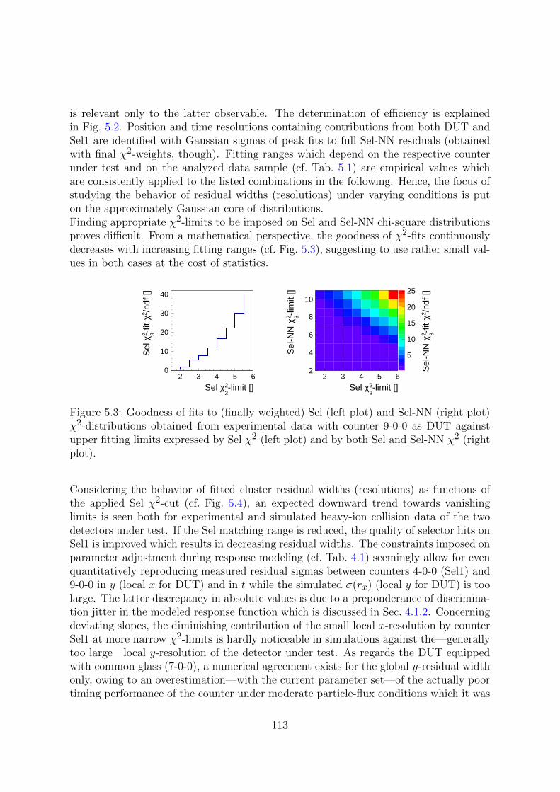
is relevant only to the latter observable. The determination of efficiency is explainedin Fig. 5.2. Position and time resolutions containing contributions from both DUT andSel1 are identified with Gaussian sigmas of peak fits to full Sel-NN residuals (obtainedwith final χ2-weights, though). Fitting ranges which depend on the respective counterunder test and on the analyzed data sample (cf. Tab. 5.1) are empirical values whichare consistently applied to the listed combinations in the following. Hence, the focus ofstudying the behavior of residual widths (resolutions) under varying conditions is puton the approximately Gaussian core of distributions.Finding appropriate χ2-limits to be imposed on Sel and Sel-NN chi-square distributionsproves difficult. From a mathematical perspective, the goodness of χ2-fits continuouslydecreases with increasing fitting ranges (cf. Fig. 5.3), suggesting to use rather small val-ues in both cases at the cost of statistics.

2 3 4 5 6

-limit []32χ Sel

0

10

20

30

40

/ndf

[]2 χ

-fit

32 χ S

el

2 3 4 5 6

-limit []32χ Sel

2

4

6

8

10-li

mit

[]32 χ

Sel

-NN

5

10

15

20

25

/ndf

[]2 χ

-fit

32 χ S

el-N

N

Figure 5.3: Goodness of fits to (finally weighted) Sel (left plot) and Sel-NN (right plot)χ2-distributions obtained from experimental data with counter 9-0-0 as DUT againstupper fitting limits expressed by Sel χ2 (left plot) and by both Sel and Sel-NN χ2 (rightplot).

Considering the behavior of fitted cluster residual widths (resolutions) as functions ofthe applied Sel χ2-cut (cf. Fig. 5.4), an expected downward trend towards vanishinglimits is seen both for experimental and simulated heavy-ion collision data of the twodetectors under test. If the Sel matching range is reduced, the quality of selector hits onSel1 is improved which results in decreasing residual widths. The constraints imposed onparameter adjustment during response modeling (cf. Tab. 4.1) seemingly allow for evenquantitatively reproducing measured residual sigmas between counters 4-0-0 (Sel1) and9-0-0 in y (local x for DUT) and in t while the simulated σ(rx) (local y for DUT) is toolarge. The latter discrepancy in absolute values is due to a preponderance of discrimina-tion jitter in the modeled response function which is discussed in Sec. 4.1.2. Concerningdeviating slopes, the diminishing contribution of the small local x-resolution by counterSel1 at more narrow χ2-limits is hardly noticeable in simulations against the—generallytoo large—local y-resolution of the detector under test. As regards the DUT equippedwith common glass (7-0-0), a numerical agreement exists for the global y-residual widthonly, owing to an overestimation—with the current parameter set—of the actually poortiming performance of the counter under moderate particle-flux conditions which it was

113

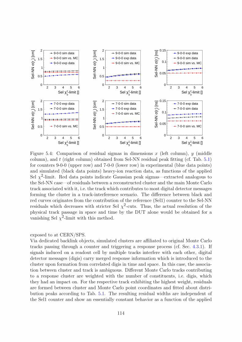
2 3 4 5 6

-limit []32χ Sel

0

0.5

1

1.5

2

) [c

m]

x(rσ

Sel

-NN

9-0-0 sim data

9-0-0 sim vs. MC

9-0-0 exp data

2 3 4 5 6

-limit []32χ Sel

0

0.5

1

1.5

2

) [c

m]

y(rσ

Sel

-NN

9-0-0 sim data

9-0-0 exp data

9-0-0 sim vs. MC

2 3 4 5 6

-limit []32χ Sel

0

0.05

0.1

0.15

) [n

s]t

(rσ S

el-N

N

9-0-0 exp data

9-0-0 sim data

9-0-0 sim vs. MC

2 3 4 5 6

-limit []32χ Sel

0

0.5

1

1.5

2

) [c

m]

x(rσ

Sel

-NN

7-0-0 exp data

7-0-0 sim data

7-0-0 sim vs. MC

2 3 4 5 6

-limit []32χ Sel

0

0.5

1

1.5

2

) [c

m]

y(rσ

Sel

-NN

7-0-0 sim data

7-0-0 exp data

7-0-0 sim vs. MC

2 3 4 5 6

-limit []32χ Sel

0

0.05

0.1

0.15

) [n

s]t

(rσ S

el-N

N

7-0-0 exp data

7-0-0 sim data

7-0-0 sim vs. MC

Figure 5.4: Comparison of residual sigmas in dimensions x (left column), y (middlecolumn), and t (right column) obtained from Sel-NN residual peak fitting (cf. Tab. 5.1)for counters 9-0-0 (upper row) and 7-0-0 (lower row) in experimental (blue data points)and simulated (black data points) heavy-ion reaction data, as functions of the appliedSel χ2-limit. Red data points indicate Gaussian peak sigmas—extracted analogous tothe Sel-NN case—of residuals between a reconstructed cluster and the main Monte Carlotrack associated with it, i.e. the track which contributes to most digital detector messagesforming the cluster in a track-interference scenario. The difference between black andred curves originates from the contribution of the reference (Sel1) counter to the Sel-NNresiduals which decreases with stricter Sel χ2-cuts. Thus, the actual resolution of thephysical track passage in space and time by the DUT alone would be obtained for avanishing Sel χ2-limit with this method.

exposed to at CERN/SPS.Via dedicated backlink objects, simulated clusters are affiliated to original Monte Carlotracks passing through a counter and triggering a response process (cf. Sec. 4.3.1). Ifsignals induced on a readout cell by multiple tracks interfere with each other, digitaldetector messages (digis) carry merged response information which is introduced to thecluster upon formation from correlated digis in time and space. In this case, the associa-tion between cluster and track is ambiguous. Different Monte Carlo tracks contributingto a response cluster are weighted with the number of constituents, i.e. digis, whichthey had an impact on. For the respective track exhibiting the highest weight, residualsare formed between cluster and Monte Carlo point coordinates and fitted about distri-bution peaks according to Tab. 5.1. The resulting residual widths are independent ofthe Sel1 counter and show an essentially constant behavior as a function of the applied

114

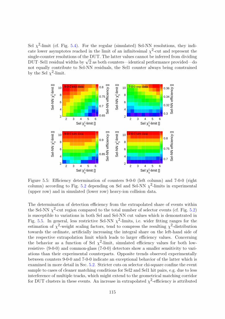
Sel χ2-limit (cf. Fig. 5.4). For the regular (simulated) Sel-NN resolutions, they indi-cate lower asymptotes reached in the limit of an infinitesimal χ2-cut and represent thesingle-counter resolutions of the DUT. The latter values cannot be inferred from dividingDUT–Sel1 residual widths by

√2 as both counters—identical performance provided—do

not equally contribute to Sel-NN residuals, the Sel1 counter always being constrainedby the Sel χ2-limit.

2 3 4 5 6

-limit []32χ Sel

2

4

6

8

10

-lim

it []

32 χ S

el-N

N

0.65

0.7

0.75

0.8

Sel

-NN

effi

cien

cy []9-0-0 exp data

2 3 4 5 6

-limit []32χ Sel

2

4

6

8

10

-lim

it []

32 χ S

el-N

N

0.3

0.32

0.34

0.36

Sel

-NN

effi

cien

cy []7-0-0 exp data

2 3 4 5 6

-limit []32χ Sel

2

4

6

8

10

-lim

it []

32 χ S

el-N

N

0.85

0.9

Sel

-NN

effi

cien

cy []9-0-0 sim data

2 3 4 5 6

-limit []32χ Sel

2

4

6

8

10

-lim

it []

32 χ S

el-N

N

0.7

0.75

0.8

Sel

-NN

effi

cien

cy []7-0-0 sim data

Figure 5.5: Efficiency determination of counters 9-0-0 (left column) and 7-0-0 (rightcolumn) according to Fig. 5.2 depending on Sel and Sel-NN χ2-limits in experimental(upper row) and in simulated (lower row) heavy-ion collision data.

The determination of detection efficiency from the extrapolated share of events withinthe Sel-NN χ2-cut region compared to the total number of selector events (cf. Fig. 5.2)is susceptible to variations in both Sel and Sel-NN cut values which is demonstrated inFig. 5.5. In general, less restrictive Sel-NN χ2-limits, i.e. wider fitting ranges for theestimation of χ2-weight scaling factors, tend to compress the resulting χ2-distributiontowards the ordinate, artificially increasing the integral share on the left-hand side ofthe respective extrapolation limit which leads to larger efficiency values. Concerningthe behavior as a function of Sel χ2-limit, simulated efficiency values for both low-resistive- (9-0-0) and common-glass (7-0-0) detectors show a smaller sensitivity to vari-ations than their experimental counterparts. Opposite trends observed experimentallybetween counters 9-0-0 and 7-0-0 indicate an exceptional behavior of the latter which isexamined in more detail in Sec. 5.2. Stricter cuts on selector chi-square confine the eventsample to cases of cleaner matching conditions for Sel2 and Sel1 hit pairs, e.g. due to lessinterference of multiple tracks, which might extend to the geometrical matching corridorfor DUT clusters in these events. An increase in extrapolated χ2-efficiency is attributed

115

to a reduction of non-Gaussian tails in Sel-NN residuals which are partially caused byresponse interference on the DUT, assuming that any response tails on the Sel1 counterare suppressed by the cut on Sel χ2—at least within the considered range—and do notenter into DUT–Sel1 residuals. Possibly owing to more pronounced tails in simulatedresiduals even in the absence of signal interference effects (cf. Fig. 4.6), a change inselector χ2-limit is not coupled to a strong variation in efficiency here. Too narrow Selχ2-limits, however, could introduce bias to the extrapolation method by providing aninsufficiently large fitting range to account for the tail behavior of the χ2-distribution,both for simulated and experimental data, an argument which also holds for the Sel-NNcase.In terms of absolute efficiency scales, higher values are obtained for the virtual and realprototype equipped with low-resistive glass (9-0-0) as anticipated. The low numbers re-ceived for the measured common-glass counter (7-0-0) are surprising at moderate mean

particle fluxes on the surface of about 1.3 kHz/cm2 but could be explained with the spikein beam intensity preceding every recorded spill in the test beam at CERN/SPS. Regard-ing efficiency values in the 70 % range for counter 9-0-0, no cut on cluster multiplicityis applied in the present case yet, i.e. residual distortions due to response interferencewhich significantly reduce χ2-efficiency are not suppressed. In the subsequent anal-ysis, identical χ2-limits are used for all scenarios to ensure comparability. From theabove discussion, cuts on Sel chi-square at 2.5 and on Sel-NN chi-square at 5.0 seemreasonable, keeping in mind the related systematic uncertainties. Assuming perfect χ2-distributions, about 52.4 % and 82.8 % of entries in a corresponding histogram wouldbe located in the respective cut region while underlying response residuals—if purelyGaussian in shape—would be constrained to intervals of ±

√2.5σ and ±

√5.0σ about a

mean of zero, respectively.

5.2 Track-interference bias on detector response

Multiple particles traversing the counter surface within a short time interval have achance to trigger interfering response processes which influence detector performance.In principal, this phenomenon is independent of the incident particle flux on the counterand can occur also at low beam–target interaction rates. The critical factor is the meanmultiplicity of reaction secondaries which the counter is exposed to in single collisionevents, a quantity that varies with beam kinetic energy and size of the colliding nuclei.In a Monte Carlo simulation, the number of tracks contributing to the generation ofa response cluster is known and could directly be used as an indicator for signal in-terference. Experimentally, for the test-beam setup at CERN/SPS in particular, themeasured cluster multiplicity on the large-area selector counter 3-0-0 allows for an as-sessment of the multi-hit conditions which the remaining counters positioned behindare confronted with in a given event. With respect to straight-line tracks originatingfrom the target, the active area of the Sel2 counter shadows the readout planes of thetwo detectors under test and the Sel1 counter in the back, except for an approximately1 cm wide vertical band on 9-0-0 in positive global x. Consequently, assuming a high

116

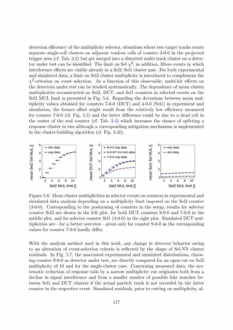
detection efficiency of the multiplicity selector, situations where two target tracks createseparate single-cell clusters on adjacent readout cells of counter 3-0-0 in the projectedtrigger area (cf. Tab. 3.2) but get merged into a distorted multi-track cluster on a detec-tor under test can be identified. The limit on Sel χ2, in addition, filters events in whichinterference effects are visible already in a Sel2–Sel1 cluster pair. For both experimentaland simulated data, a limit on Sel2 cluster multiplicity is introduced to complement theχ2-criterion on event selection. As a function of this observable, multi-hit effects onthe detectors under test can be studied systematically. The dependence of mean clustermultiplicities reconstructed on Sel2, DUT, and Sel1 counters in selected events on theSel2 MUL limit is presented in Fig. 5.6. Regarding the deviations between mean mul-tiplicity values obtained for counters 7-0-0 (DUT) and 4-0-0 (Sel1) in experiment andsimulation, the former offset might result from the relatively low efficiency measuredfor counter 7-0-0 (cf. Fig. 5.5) and the latter difference could be due to a dead cell inthe center of the real counter (cf. Tab. 3.4) which increases the chance of splitting aresponse cluster in two although a corresponding mitigation mechanism is implementedin the cluster-building algorithm (cf. Fig. 3.20).

2 4 6 8 10

Sel2 MUL limit []

1

2

3

4

5

mea

n S

el2

Sel

MU

L [] sim data

exp data

2 4 6 8 10

Sel2 MUL limit []

1

2

3

4

5

mea

n D

UT

Sel

MU

L []

9-0-0 exp data

9-0-0/7-0-0 sim data

7-0-0 exp data

2 4 6 8 10

Sel2 MUL limit []

1

2

3

4

5

mea

n S

el1

Sel

MU

L [] exp data

sim data

Figure 5.6: Mean cluster multiplicities in selector events on counters in experimental andsimulated data analysis depending on a multiplicity limit imposed on the Sel2 counter(3-0-0). Corresponding to the positioning of counters in the setup, results for selectorcounter Sel2 are shown in the left plot, for both DUT counters 9-0-0 and 7-0-0 in themiddle plot, and for selector counter Sel1 (4-0-0) in the right plot. Simulated DUT mul-tiplicities are—for a better overview—given only for counter 9-0-0 as the correspondingvalues for counter 7-0-0 hardly differ.

With the analysis method used in this work, any change in detector behavior owingto an alteration of event-selection criteria is reflected by the shape of Sel-NN clusterresiduals. In Fig. 5.7, the associated experimental and simulated distributions, choos-ing counter 9-0-0 as detector under test, are directly compared for an open cut on Sel2multiplicity of 10 and for the single-cluster case. Concerning measured data, the sys-tematic reduction of response tails by a narrow multiplicity cut originates both from adecline in signal interference and from a smaller number of possible fake matches be-tween Sel1 and DUT clusters if the actual particle track is not recorded by the lattercounter in the respective event. Simulated residuals, prior to cutting on multiplicity, al-

117

Mean 0.0009883− Sigma 0.5277

20− 10− 0 10 20

[cm]x Sel-NN r

1

10

210

310

410Mean 0.0009883− Sigma 0.5277

Mean 0.004096Sigma 0.46Mean 0.004096Sigma 0.46

9-0-0 expMean 0.0007848− Sigma 0.5034

20− 10− 0 10 20

[cm]y Sel-NN r

1

10

210

310

410Mean 0.0007848− Sigma 0.5034

Mean 0.001883− Sigma 0.4956Mean 0.001883− Sigma 0.4956

9-0-0 expMean 05−7.883e− Sigma 0.06509

2− 0 2

[ns]t Sel-NN r

1

10

210

310

410Mean 05−7.883e− Sigma 0.06509

Mean 0.0006678− Sigma 0.05829Mean 0.0006678− Sigma 0.05829

9-0-0 exp

Mean 05−5.099e− Sigma 0.7857

20− 10− 0 10 20

[cm]x Sel-NN r

1

10

210

310

410

510Mean 05−5.099e− Sigma 0.7857

Mean 05−6.817e− Sigma 0.767Mean 05−6.817e− Sigma 0.767

9-0-0 simMean 0.0001025− Sigma 0.5229

20− 10− 0 10 20

[cm]y Sel-NN r

1

10

210

310

410

510Mean 0.0001025− Sigma 0.5229

Mean 0.0009905− Sigma 0.4966Mean 0.0009905− Sigma 0.4966

9-0-0 simMean 06− 4.064eSigma 0.06627

2− 0 2

[ns]t Sel-NN r

1

10

210

310

410

510Mean 06− 4.064eSigma 0.06627

Mean 05−8.573e− Sigma 0.06494Mean 05−8.573e− Sigma 0.06494

9-0-0 sim

Figure 5.7: Comparison of Sel-NN residuals in x (left column), y (middle column), andt (right column) for experimental (upper row) and simulated (lower row) 9-0-0 datawith a cluster-multiplicity limit on the Sel2 counter (3-0-0) of 10 (blue histograms) andof 1 (dark green histograms) in place. Statistics boxes display means and sigmas ofGaussian peak fits (cf. Tab. 5.1) for both cases. In addition to a statistical decrease inhistogram entries which results from constraining event selection by a strict MUL limit,structures in the residuals attributed to track interference and—in case of local counterinefficiencies—false NN attributions of DUT clusters to a selector prediction are largelysuppressed.

most exclusively comprise interference-induced tails as the counter parametrization withlow-resistive glass yields a measurable detector response—not a clean one, though—forclose to 100 % of incident tracks at these particle fluxes (cf. Fig. 4.10). The overestima-tion of local y-residual widths in simulations which—for the DUT—contributes to theglobal x-residual has been discussed. As regards the improvement of resolutions, i.e.the decrease of fit-extracted residual peak widths between the two cut conditions, largerdifferences in the timing dimensions y (global x) and t are obtained with experimentaldata. While a reduction of interference effects also occurs for simulated data, primarilyin distribution tails, residual centers are affected to a lesser degree. In the responsemodel, interfering signals are treated independently up to and including signal-edge dis-crimination, to then be merged if ToT ranges overlap. Leading-edge information of thelatter signal is lost completely. In reality, interfering response processes can influenceeach other already at the level of signal formation with the result that they are jointlyreflected in the final leading-edge measurement, yielding smaller discrepancies betweenthe passage of original particles through the detector and reconstructed cluster coordi-

118

nates. This could explain the greater susceptibility of experimental residual centers tointerference suppression, apart from the presence of NN mismatches in this case.

Mean 0.008335− Sigma 1.232

20− 10− 0 10 20

[cm]x Sel-NN r

1

10

210

310

Mean 0.008335− Sigma 1.232

Mean 0.002488− Sigma 1.04Mean 0.002488− Sigma 1.04

7-0-0 expMean 0.004709Sigma 0.724

20− 10− 0 10 20

[cm]y Sel-NN r

1

10

210

310

Mean 0.004709Sigma 0.724

Mean 0.00282Sigma 0.6618Mean 0.00282Sigma 0.6618

7-0-0 expMean 05− 1.159eSigma 0.08999

2− 0 2

[ns]t Sel-NN r

1

10

210

310

Mean 05− 1.159eSigma 0.08999

Mean 0.0001443− Sigma 0.07425Mean 0.0001443− Sigma 0.07425

7-0-0 exp

Mean 0.0009994− Sigma 0.9233

20− 10− 0 10 20

[cm]x Sel-NN r

1

10

210

310

410

510 Mean 0.0009994− Sigma 0.9233

Mean 0.00198− Sigma 0.8855Mean 0.00198− Sigma 0.8855

7-0-0 simMean 0.0005102Sigma 0.7155

20− 10− 0 10 20

[cm]y Sel-NN r

1

10

210

310

410

510Mean 0.0005102Sigma 0.7155

Mean 0.0006581Sigma 0.6766Mean 0.0006581Sigma 0.6766

7-0-0 simMean 05− 8.496eSigma 0.07643

2− 0 2

[ns]t Sel-NN r

1

10

210

310

410

510Mean 05− 8.496eSigma 0.07643

Mean 0.0001704− Sigma 0.0736Mean 0.0001704− Sigma 0.0736

7-0-0 sim

Figure 5.8: Comparison of Sel-NN residuals in x (left column), y (middle column), andt (right column) for experimental (upper row) and simulated (lower row) 7-0-0 datawith a cluster-multiplicity limit on the Sel2 counter (3-0-0) of 10 (blue histograms) andof 1 (dark green histograms) in place. Statistics boxes display means and sigmas ofGaussian peak fits (cf. Tab. 5.1) for both cases. In addition to a statistical decrease inhistogram entries which results from constraining event selection by a strict MUL limit,structures in the residuals attributed to track interference and—in case of local counterinefficiencies—false NN attributions of DUT clusters to a selector prediction are largelysuppressed. Note the second peak in the experimental time residual (upper right plot)which is not filtered out by cutting on Sel2 multiplicity and which is assumed to originatefrom signal reflections at the locally positive cell end (cf. Fig. 3.4). The bump visible inthe negative axis range of the low-multiplicity global x-residual (upper left plot) resultsfrom the corresponding impact of reflections on the reconstruction of local y.

The residual behavior of common-glass counters is shown in Fig. 5.8. Both the real andthe simulated prototype exhibit detection inefficiencies at the given mean particle fluxesof 1.3 and 1.0 kHz/cm2, respectively, which are responsible for a prominent backgroundfrom nearest-neighbor mismatches in residual spectra that also causes a broadening ofdistribution centers. Plateau ranges in position residuals differ as some peripheral read-out cells are declared dead in experimental data (cf. Tab. 3.4). In the simulated globaly-residual, prior to applying the multiplicity cut, the discrete local x-coordinates of read-out cells are indicated on which a substitute cluster for the missing true NN match iscentered. Allowing for a single cluster on selector counter 3-0-0 only does not completely

119

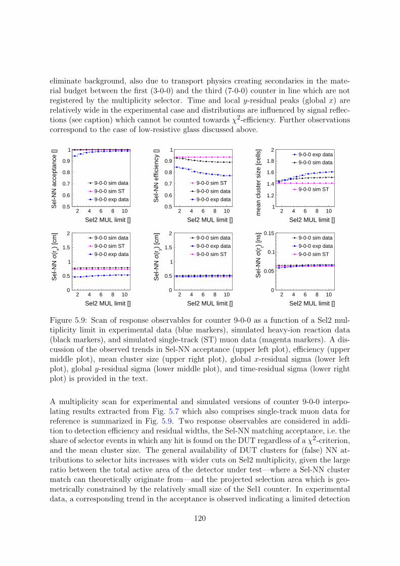
eliminate background, also due to transport physics creating secondaries in the mate-rial budget between the first (3-0-0) and the third (7-0-0) counter in line which are notregistered by the multiplicity selector. Time and local y-residual peaks (global x) arerelatively wide in the experimental case and distributions are influenced by signal reflec-tions (see caption) which cannot be counted towards χ2-efficiency. Further observationscorrespond to the case of low-resistive glass discussed above.

2 4 6 8 10

Sel2 MUL limit []

0.5

0.6

0.7

0.8

0.9

1

Sel

-NN

acc

epta

nce

[]

9-0-0 sim data

9-0-0 sim ST

9-0-0 exp data

2 4 6 8 10

Sel2 MUL limit []

0.5

0.6

0.7

0.8

0.9

1 S

el-N

N e

ffici

ency

[]

9-0-0 sim ST

9-0-0 sim data

9-0-0 exp data

2 4 6 8 10

Sel2 MUL limit []

1

1.2

1.4

1.6

1.8

2

mea

n cl

uste

r si

ze [c

ells

]

9-0-0 exp data

9-0-0 sim data

9-0-0 sim ST

2 4 6 8 10

Sel2 MUL limit []

0

0.5

1

1.5

2

) [c

m]

x(rσ

Sel

-NN

9-0-0 sim data

9-0-0 sim ST

9-0-0 exp data

2 4 6 8 10

Sel2 MUL limit []

0

0.5

1

1.5

2

) [c

m]

y(rσ

Sel

-NN

9-0-0 sim data

9-0-0 exp data

9-0-0 sim ST

2 4 6 8 10

Sel2 MUL limit []

0

0.05

0.1

0.15

) [n

s]t

(rσ S

el-N

N

9-0-0 sim data

9-0-0 exp data

9-0-0 sim ST

Figure 5.9: Scan of response observables for counter 9-0-0 as a function of a Sel2 mul-tiplicity limit in experimental data (blue markers), simulated heavy-ion reaction data(black markers), and simulated single-track (ST) muon data (magenta markers). A dis-cussion of the observed trends in Sel-NN acceptance (upper left plot), efficiency (uppermiddle plot), mean cluster size (upper right plot), global x-residual sigma (lower leftplot), global y-residual sigma (lower middle plot), and time-residual sigma (lower rightplot) is provided in the text.

A multiplicity scan for experimental and simulated versions of counter 9-0-0 interpo-lating results extracted from Fig. 5.7 which also comprises single-track muon data forreference is summarized in Fig. 5.9. Two response observables are considered in addi-tion to detection efficiency and residual widths, the Sel-NN matching acceptance, i.e. theshare of selector events in which any hit is found on the DUT regardless of a χ2-criterion,and the mean cluster size. The general availability of DUT clusters for (false) NN at-tributions to selector hits increases with wider cuts on Sel2 multiplicity, given the largeratio between the total active area of the detector under test—where a Sel-NN clustermatch can theoretically originate from—and the projected selection area which is geo-metrically constrained by the relatively small size of the Sel1 counter. In experimentaldata, a corresponding trend in the acceptance is observed indicating a limited detection

120

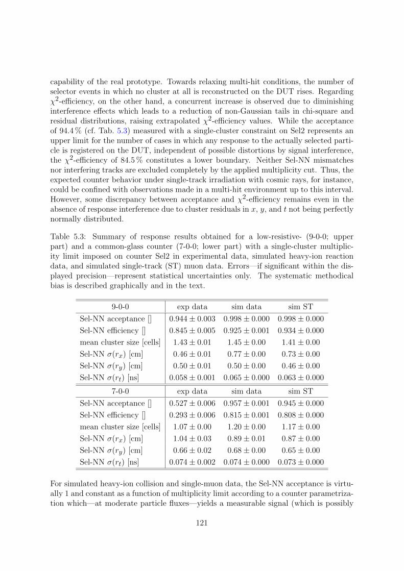
capability of the real prototype. Towards relaxing multi-hit conditions, the number ofselector events in which no cluster at all is reconstructed on the DUT rises. Regardingχ2-efficiency, on the other hand, a concurrent increase is observed due to diminishinginterference effects which leads to a reduction of non-Gaussian tails in chi-square andresidual distributions, raising extrapolated χ2-efficiency values. While the acceptanceof 94.4 % (cf. Tab. 5.3) measured with a single-cluster constraint on Sel2 represents anupper limit for the number of cases in which any response to the actually selected parti-cle is registered on the DUT, independent of possible distortions by signal interference,the χ2-efficiency of 84.5 % constitutes a lower boundary. Neither Sel-NN mismatchesnor interfering tracks are excluded completely by the applied multiplicity cut. Thus, theexpected counter behavior under single-track irradiation with cosmic rays, for instance,could be confined with observations made in a multi-hit environment up to this interval.However, some discrepancy between acceptance and χ2-efficiency remains even in theabsence of response interference due to cluster residuals in x, y, and t not being perfectlynormally distributed.

Table 5.3: Summary of response results obtained for a low-resistive- (9-0-0; upperpart) and a common-glass counter (7-0-0; lower part) with a single-cluster multiplic-ity limit imposed on counter Sel2 in experimental data, simulated heavy-ion reactiondata, and simulated single-track (ST) muon data. Errors—if significant within the dis-played precision—represent statistical uncertainties only. The systematic methodicalbias is described graphically and in the text.

9-0-0 exp data sim data sim ST

Sel-NN acceptance [] 0.944± 0.003 0.998± 0.000 0.998± 0.000

Sel-NN efficiency [] 0.845± 0.005 0.925± 0.001 0.934± 0.000

mean cluster size [cells] 1.43± 0.01 1.45± 0.00 1.41± 0.00

Sel-NN σ(rx) [cm] 0.46± 0.01 0.77± 0.00 0.73± 0.00

Sel-NN σ(ry) [cm] 0.50± 0.01 0.50± 0.00 0.46± 0.00

Sel-NN σ(rt) [ns] 0.058± 0.001 0.065± 0.000 0.063± 0.000

7-0-0 exp data sim data sim ST

Sel-NN acceptance [] 0.527± 0.006 0.957± 0.001 0.945± 0.000

Sel-NN efficiency [] 0.293± 0.006 0.815± 0.001 0.808± 0.000

mean cluster size [cells] 1.07± 0.00 1.20± 0.00 1.17± 0.00

Sel-NN σ(rx) [cm] 1.04± 0.03 0.89± 0.01 0.87± 0.00

Sel-NN σ(ry) [cm] 0.66± 0.02 0.68± 0.00 0.65± 0.00

Sel-NN σ(rt) [ns] 0.074± 0.002 0.074± 0.000 0.073± 0.000

For simulated heavy-ion collision and single-muon data, the Sel-NN acceptance is virtu-ally 1 and constant as a function of multiplicity limit according to a counter parametriza-tion which—at moderate particle fluxes—yields a measurable signal (which is possibly

121

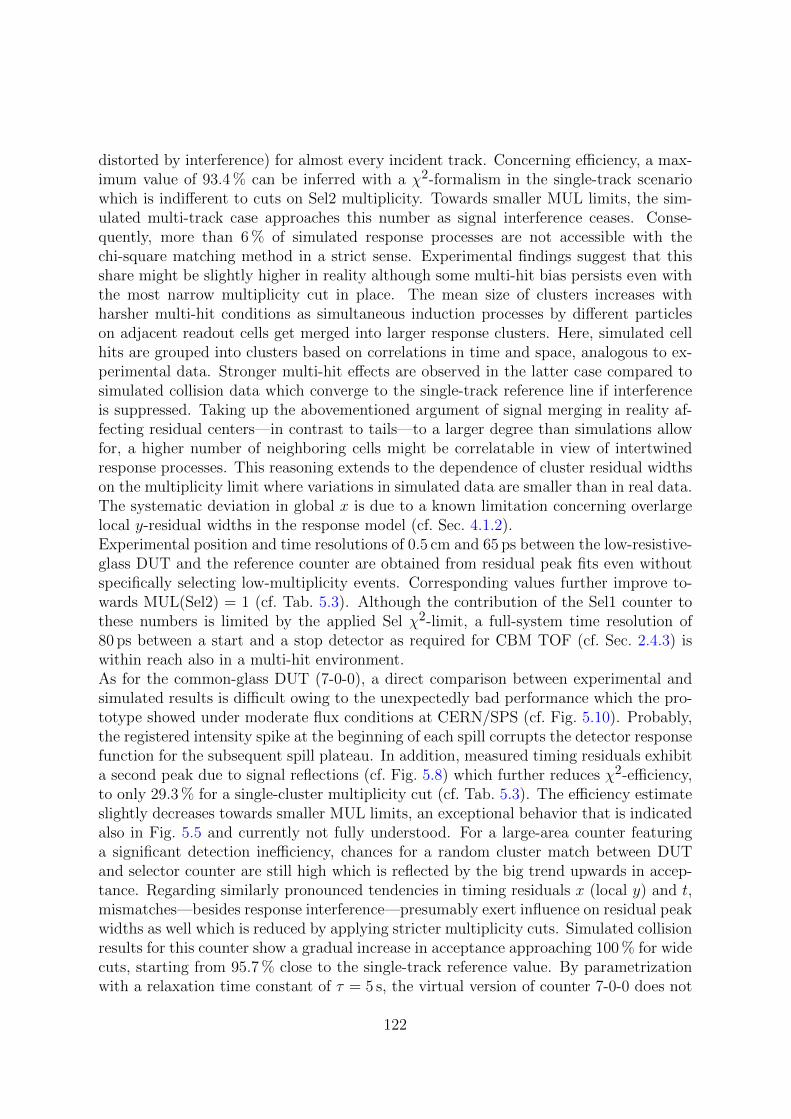
distorted by interference) for almost every incident track. Concerning efficiency, a max-imum value of 93.4 % can be inferred with a χ2-formalism in the single-track scenariowhich is indifferent to cuts on Sel2 multiplicity. Towards smaller MUL limits, the sim-ulated multi-track case approaches this number as signal interference ceases. Conse-quently, more than 6 % of simulated response processes are not accessible with thechi-square matching method in a strict sense. Experimental findings suggest that thisshare might be slightly higher in reality although some multi-hit bias persists even withthe most narrow multiplicity cut in place. The mean size of clusters increases withharsher multi-hit conditions as simultaneous induction processes by different particleson adjacent readout cells get merged into larger response clusters. Here, simulated cellhits are grouped into clusters based on correlations in time and space, analogous to ex-perimental data. Stronger multi-hit effects are observed in the latter case compared tosimulated collision data which converge to the single-track reference line if interferenceis suppressed. Taking up the abovementioned argument of signal merging in reality af-fecting residual centers—in contrast to tails—to a larger degree than simulations allowfor, a higher number of neighboring cells might be correlatable in view of intertwinedresponse processes. This reasoning extends to the dependence of cluster residual widthson the multiplicity limit where variations in simulated data are smaller than in real data.The systematic deviation in global x is due to a known limitation concerning overlargelocal y-residual widths in the response model (cf. Sec. 4.1.2).Experimental position and time resolutions of 0.5 cm and 65 ps between the low-resistive-glass DUT and the reference counter are obtained from residual peak fits even withoutspecifically selecting low-multiplicity events. Corresponding values further improve to-wards MUL(Sel2) = 1 (cf. Tab. 5.3). Although the contribution of the Sel1 counter tothese numbers is limited by the applied Sel χ2-limit, a full-system time resolution of80 ps between a start and a stop detector as required for CBM TOF (cf. Sec. 2.4.3) iswithin reach also in a multi-hit environment.As for the common-glass DUT (7-0-0), a direct comparison between experimental andsimulated results is difficult owing to the unexpectedly bad performance which the pro-totype showed under moderate flux conditions at CERN/SPS (cf. Fig. 5.10). Probably,the registered intensity spike at the beginning of each spill corrupts the detector responsefunction for the subsequent spill plateau. In addition, measured timing residuals exhibita second peak due to signal reflections (cf. Fig. 5.8) which further reduces χ2-efficiency,to only 29.3 % for a single-cluster multiplicity cut (cf. Tab. 5.3). The efficiency estimateslightly decreases towards smaller MUL limits, an exceptional behavior that is indicatedalso in Fig. 5.5 and currently not fully understood. For a large-area counter featuringa significant detection inefficiency, chances for a random cluster match between DUTand selector counter are still high which is reflected by the big trend upwards in accep-tance. Regarding similarly pronounced tendencies in timing residuals x (local y) and t,mismatches—besides response interference—presumably exert influence on residual peakwidths as well which is reduced by applying stricter multiplicity cuts. Simulated collisionresults for this counter show a gradual increase in acceptance approaching 100 % for widecuts, starting from 95.7 % close to the single-track reference value. By parametrizationwith a relaxation time constant of τ = 5 s, the virtual version of counter 7-0-0 does not

122

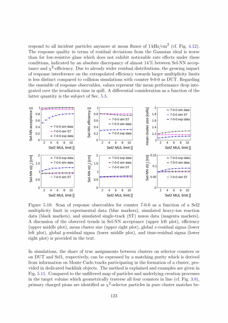
respond to all incident particles anymore at mean fluxes of 1 kHz/cm2 (cf. Fig. 4.12).The response quality in terms of residual deviations from the Gaussian ideal is worsethan for low-resistive glass which does not exhibit noticeable rate effects under theseconditions, indicated by an absolute discrepancy of almost 14 % between Sel-NN accep-tance and χ2-efficiency. Due to already wider residual distributions, the growing impactof response interference on the extrapolated efficiency towards larger multiplicity limitsis less distinct compared to collision simulations with counter 9-0-0 as DUT. Regardingthe ensemble of response observables, values represent the mean performance drop inte-grated over the irradiation time in spill. A differential consideration as a function of thelatter quantity is the subject of Sec. 5.3.

2 4 6 8 10

Sel2 MUL limit []

0

0.2

0.4

0.6

0.8

1

Sel

-NN

acc

epta

nce

[]

7-0-0 sim data

7-0-0 sim ST

7-0-0 exp data

2 4 6 8 10

Sel2 MUL limit []

0

0.2

0.4

0.6

0.8

1

Sel

-NN

effi

cien

cy []

7-0-0 sim ST

7-0-0 sim data

7-0-0 exp data

2 4 6 8 10

Sel2 MUL limit []

1

1.2

1.4

1.6

1.8

2

mea

n cl

uste

r si

ze [c

ells

]

7-0-0 sim data

7-0-0 sim ST

7-0-0 exp data

2 4 6 8 10

Sel2 MUL limit []

0

0.5

1

1.5

2

) [c

m]

x(rσ

Sel

-NN

7-0-0 exp data

7-0-0 sim data

7-0-0 sim ST

2 4 6 8 10

Sel2 MUL limit []

0

0.5

1

1.5

2

) [c

m]

y(rσ

Sel

-NN

7-0-0 exp data

7-0-0 sim data

7-0-0 sim ST

2 4 6 8 10

Sel2 MUL limit []

0

0.05

0.1

0.15

) [n

s]t

(rσ S

el-N

N

7-0-0 exp data

7-0-0 sim data

7-0-0 sim ST

Figure 5.10: Scan of response observables for counter 7-0-0 as a function of a Sel2multiplicity limit in experimental data (blue markers), simulated heavy-ion reactiondata (black markers), and simulated single-track (ST) muon data (magenta markers).A discussion of the observed trends in Sel-NN acceptance (upper left plot), efficiency(upper middle plot), mean cluster size (upper right plot), global x-residual sigma (lowerleft plot), global y-residual sigma (lower middle plot), and time-residual sigma (lowerright plot) is provided in the text.

In simulations, the share of true assignments between clusters on selector counters oron DUT and Sel1, respectively, can be expressed by a matching purity which is derivedfrom information on Monte Carlo tracks participating in the formation of a cluster, pro-vided in dedicated backlink objects. The method is explained and examples are given inFig. 5.11. Compared to the unfiltered map of particles and underlying creation processesin the target volume which geometrically traverse all four counters in line (cf. Fig. 3.8),primary charged pions are identified as χ2-selector particles in pure cluster matches be-

123

tween Sel2 and Sel1 more frequently, their relative share increasing from 52 % to 68 %.At the same time, clusters created by electron–positron or proton tracks are selectedless often due to trajectory deflections in the setup by multiple scattering in the formercase and the comparatively low velocity of protons in the latter. The chance to triggera clean detector response in accordance with the Sel χ2-criterion is highest for the ear-liest hits on counters in an event which are attributed to fast pions. As a function ofmultiplicity limit on counter Sel2, the high selector purity obtained with the default Selχ2-cut (2.5) in a simulated collision scenario minimally decreases. The same applies tothe Sel-NN purity—a pure Sel match provided—if counter 9-0-0 serves as detector undertest. Owing to the reduced detection efficiency which a common-glass parametrizationyields at the considered particle fluxes, the Sel-NN acceptance grows with more challeng-ing multi-hit conditions (cf. Fig. 5.10) at the cost of increasingly impure cluster matchesbetween counter 7-0-0 and selectors.

0.00 0.01

0.00 0.03

0.00 0.06

0.00 0.06

0.00 0.00 0.13

0.00 0.01 0.33

0.01 0.01 0.35

HADR DCAY PAIR PRIM

creation process []

-Κ

+Κ

-e

+e

p

+π

-π

sel

ecto

r pa

rtic

le []

0

0.1

0.2

0.3

2 4 6 8 10

Sel2 MUL limit []

0.5

0.6

0.7

0.8

0.9

1

Sel

pur

ity []

2 4 6 8 10

Sel2 MUL limit []

0.5

0.6

0.7

0.8

0.9

1

Sel

-NN

pur

ity []

9-0-0

7-0-0

Figure 5.11: Considerations on matching purity between clusters on selector countersSel2 and Sel1 and between the selector cluster pair and the NN cluster on DUT. If a phys-ical Monte Carlo track (detector noise excluded) contributes to selector-cluster formationboth on Sel2 and on Sel1, the selector cluster pair is considered a pure match. Creationprocesses of such selector particles in the high-multiplicity case of MUL(Sel2) ≤ 10—hereadditionally constrained by requesting a track origin in the target volume (no require-ment for matching purity)—are depicted in the left plot (normalized contributions upto a limit of 0.5 % are not shown; cf. Fig. 3.8). If one of potentially several interferingMonte Carlo tracks contributing to both selector clusters also participates in the forma-tion of the NN cluster on DUT, the NN matching between selector counters and DUTis considered pure as well. The dependence of selector purity (middle plot) and the de-pendence of DUT-matching purity (right plot) on a Sel2 multiplicity limit demonstratehigher probabilities for a mismatch the more tracks irradiate the setup simultaneously,assessed with cluster multiplicity. This effect is more pronounced for counter 7-0-0 (bluemarkers) which features an intrinsic inefficiency at fluxes under consideration due to itsconstruction with common glass plates.

It should be noted that a separate alignment of residual peaks and an independent es-timation of Sel and Sel-NN χ2-weights were conducted for every data point obtainedunder a different multiplicity cut in a given experimental/simulated scenario.

124

5.3 Rate effects under continuous irradiation

The detector response function of an MRPC degrades with irradiation time dependingon the rate at which the electric field locally breaks down due to avalanche formationtriggered by incident charged particles and on the rate at which avalanche charges ac-cumulating on opposing glass plates dissipate (cf. Sec. 2.4.2). The latter mechanism oflocal field recovery via compensation currents through the external high-voltage supplyoccurs on a relaxation time scale τMRPC which is characteristic of the glass plates thata counter is equipped with, varying with resistivity. Thus, the response behavior of acommon-glass detector with typical recovery times of the order of seconds is expectedto show a measurable degradation effect already at relatively low fluxes on the countersurface of about 1 kHz/cm2 (cf. Fig. 4.12 for a simulated projection). In fact, time av-erages of response observables studied under different multi-hit conditions in Sec. 5.2indicate a significant performance drop of counter 7-0-0 in experimental results fromCERN/SPS at these fluxes, exceeding quantitative expectations from simulations byfar. This discrepancy is primarily attributed to the spike in beam intensity precedingaccelerator spills (cf. Fig. 3.5) which causes the response function to severely deteriorateprior to recording data from the subsequent quasi-trapezoidal spill structure, under bi-ased initial conditions. Utilizing the absence of detector noise in the diamond positionedin beam ahead of the target, alternating periods of beam on target and breaks betweenspills in an accelerator cycle can be easily identified. The distance of the current meanevent time, obtained by averaging over reconstructed clusters on all counters, with re-spect to the start time of the ongoing spill, which is reset if the gap to the previousevent exceeds an adjustable interval, is considered the time in spill. Regarding responseobservables as a function of this quantity allows for a differential examination of perfor-mance degradation in time. In the following, it is assumed that the two selector countersdesigned and modeled with low-resistive glass do not exhibit rate effects at the moderateparticle fluxes under consideration. Concerning the necessary centering of residual dis-tributions about zero for the χ2-matching method to be applicable and the estimationof χ2-weights in the three response dimensions, readjustments need to be executed ifthe response function varies with increasing time in spill. In the case of common glass,this is actually required and done for simulated data but refrained from in the analysisof the experimental sample due to statistical constraints. For the latter reason, an openmultiplicity cut is used throughout this section.The share of selector events in which any cluster is found on the detector under test, i.e.the Sel-NN acceptance, is presented in Fig. 5.12, contrasting real and virtual prototypesbuilt with both types of glass, low-resistive (9-0-0) and common (7-0-0). Data pointsin single TIS (time in spill) bins are derived from averages over multiple spills. Owingto random cluster matches between a partially inefficient DUT and the Sel1 counter ina multi-hit environment (cf. Sec. 5.2), the obtained numbers are relatively high, alsofor common glass where clear trends are visible indicating a decreasing availability ofmatching candidates on the DUT surface as time in spill progresses. Given that averagetrack multiplicities on counters per collision event are not subject to change during spill,the effect can be attributed to an increasing detection inefficiency of the common-glass

125

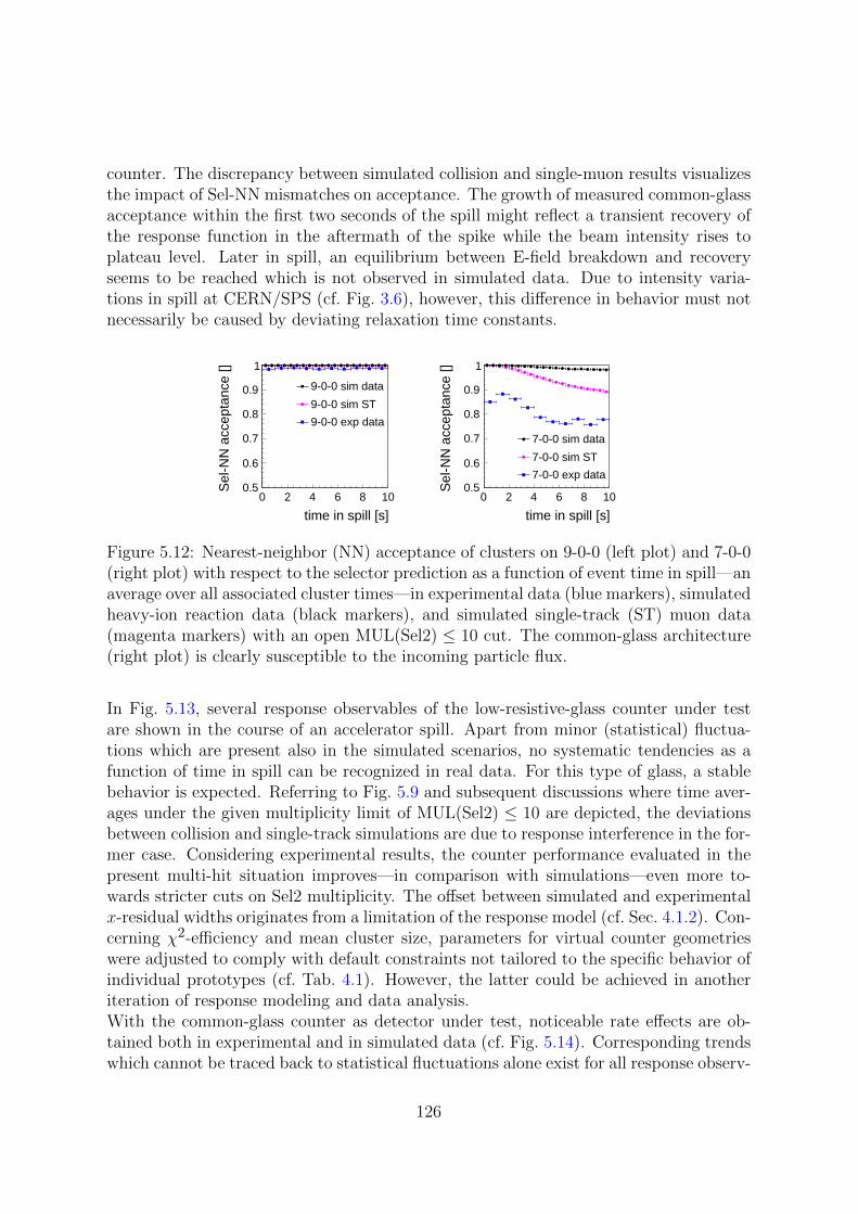
counter. The discrepancy between simulated collision and single-muon results visualizesthe impact of Sel-NN mismatches on acceptance. The growth of measured common-glassacceptance within the first two seconds of the spill might reflect a transient recovery ofthe response function in the aftermath of the spike while the beam intensity rises toplateau level. Later in spill, an equilibrium between E-field breakdown and recoveryseems to be reached which is not observed in simulated data. Due to intensity varia-tions in spill at CERN/SPS (cf. Fig. 3.6), however, this difference in behavior must notnecessarily be caused by deviating relaxation time constants.

0 2 4 6 8 10

time in spill [s]

0.5

0.6

0.7

0.8

0.9

1

Sel

-NN

acc

epta

nce

[]

9-0-0 sim data

9-0-0 sim ST

9-0-0 exp data

0 2 4 6 8 10

time in spill [s]

0.5

0.6

0.7

0.8

0.9

1

Sel

-NN

acc

epta

nce

[]7-0-0 sim data

7-0-0 sim ST

7-0-0 exp data

Figure 5.12: Nearest-neighbor (NN) acceptance of clusters on 9-0-0 (left plot) and 7-0-0(right plot) with respect to the selector prediction as a function of event time in spill—anaverage over all associated cluster times—in experimental data (blue markers), simulatedheavy-ion reaction data (black markers), and simulated single-track (ST) muon data(magenta markers) with an open MUL(Sel2) ≤ 10 cut. The common-glass architecture(right plot) is clearly susceptible to the incoming particle flux.

In Fig. 5.13, several response observables of the low-resistive-glass counter under testare shown in the course of an accelerator spill. Apart from minor (statistical) fluctua-tions which are present also in the simulated scenarios, no systematic tendencies as afunction of time in spill can be recognized in real data. For this type of glass, a stablebehavior is expected. Referring to Fig. 5.9 and subsequent discussions where time aver-ages under the given multiplicity limit of MUL(Sel2) ≤ 10 are depicted, the deviationsbetween collision and single-track simulations are due to response interference in the for-mer case. Considering experimental results, the counter performance evaluated in thepresent multi-hit situation improves—in comparison with simulations—even more to-wards stricter cuts on Sel2 multiplicity. The offset between simulated and experimentalx-residual widths originates from a limitation of the response model (cf. Sec. 4.1.2). Con-cerning χ2-efficiency and mean cluster size, parameters for virtual counter geometrieswere adjusted to comply with default constraints not tailored to the specific behavior ofindividual prototypes (cf. Tab. 4.1). However, the latter could be achieved in anotheriteration of response modeling and data analysis.With the common-glass counter as detector under test, noticeable rate effects are ob-tained both in experimental and in simulated data (cf. Fig. 5.14). Corresponding trendswhich cannot be traced back to statistical fluctuations alone exist for all response observ-

126

0 2 4 6 8 10

time in spill [s]

0.5

0.6

0.7

0.8

0.9

1

Sel

-NN

effi

cien

cy []

9-0-0 sim ST

9-0-0 sim data

9-0-0 exp data

0 2 4 6 8 10

time in spill [s]

1

1.2

1.4

1.6

1.8

2

mea

n cl

uste

r si

ze [c

ells

]

9-0-0 exp data

9-0-0 sim data

9-0-0 sim ST

0 2 4 6 8 10

time in spill [s]

1

1.5

2

2.5

3

mea

n cl

uste

r T

oT [a

.u.] 9-0-0 exp data

9-0-0 sim data

9-0-0 sim ST

0 2 4 6 8 10

time in spill [s]

0

0.5

1

1.5

2

) [c

m]

x(rσ

Sel

-NN

9-0-0 sim data

9-0-0 sim ST

9-0-0 exp data

0 2 4 6 8 10

time in spill [s]

0

0.5

1

1.5

2

) [c

m]

y(rσ

Sel

-NN

9-0-0 sim data

9-0-0 exp data

9-0-0 sim ST

0 2 4 6 8 10

time in spill [s]

0

0.05

0.1

0.15

) [n

s]t

(rσ S

el-N

N

9-0-0 sim data

9-0-0 exp data

9-0-0 sim ST

Figure 5.13: Time-in-spill (TIS) dependencies for counter 9-0-0 of extrapolated DUT ef-ficiency (upper left plot), mean cluster size (upper middle plot), average ToT of clusterdigis (upper right plot), residual sigma in x (lower left plot), residual sigma in y (lowermiddle plot), and residual sigma in t (lower right plot) in experimental data (blue mark-ers), simulated heavy-ion reaction data (black markers), and simulated single-track (ST)muon data (magenta markers) with an open MUL(Sel2) ≤ 10 cut. Due to statisticalconstraints, a TIS binning of 1 s is used for experimental data while bins for simulateddata cover TIS intervals of 0.5 s.

ables and are first experimental signs of an in-spill performance degradation measuredwith heavy-ion collision secondaries. The convergence of simulated χ2-efficiency curveswith progressing time in spill originates from the widening of residual distributions as aconsequence of decreasing signal amplitudes and increasing discrimination jitter whichreduces the impact of signal interference on already larger residual tails. Thus, themulti-track scenario approaches the single-track case in this respect. In view of theother observables, the discrepancy between simulation results under different multi-hitconditions (cf. Fig. 5.10) persists and a parallel deterioration of detector performanceoccurs in time owing to an active particle memory which records a growing numberof tracks in spill, leading to smaller values sampled from the induced charge spectrum(cf. Sec. 4.2). Regarding mean time over threshold, differences in raw-data calibrationbetween experimental and simulated data become visible, the former being corrected ontime average and the latter being aligned during memoryless parameter adjustment witha single-track irradiation of the counter surface, i.e. for TIS = 0 in the present case. Thetrend in experimental and simulated mean cluster ToT indicates diminishing signal am-plitudes on counter 7-0-0 and is reflected by corresponding tendencies in timing-residual

127

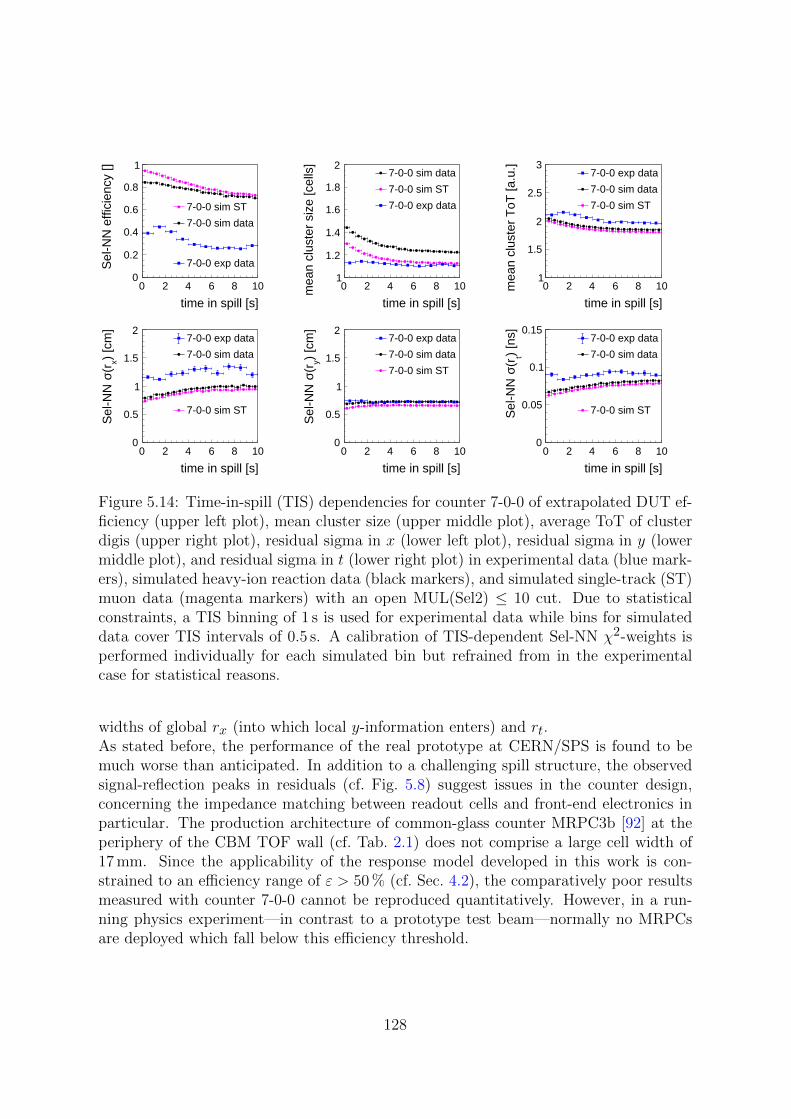
0 2 4 6 8 10

time in spill [s]

0

0.2

0.4

0.6

0.8

1

Sel

-NN

effi

cien

cy []

7-0-0 sim ST

7-0-0 sim data

7-0-0 exp data

0 2 4 6 8 10

time in spill [s]

1

1.2

1.4

1.6

1.8

2

mea

n cl

uste

r si

ze [c

ells

]

7-0-0 sim data

7-0-0 sim ST

7-0-0 exp data

0 2 4 6 8 10

time in spill [s]

1

1.5

2

2.5

3

mea

n cl

uste

r T

oT [a

.u.] 7-0-0 exp data

7-0-0 sim data

7-0-0 sim ST

0 2 4 6 8 10

time in spill [s]

0

0.5

1

1.5

2

) [c

m]

x(rσ

Sel

-NN

7-0-0 exp data

7-0-0 sim data

7-0-0 sim ST

0 2 4 6 8 10

time in spill [s]

0

0.5

1

1.5

2

) [c

m]

y(rσ

Sel

-NN

7-0-0 exp data

7-0-0 sim data

7-0-0 sim ST

0 2 4 6 8 10

time in spill [s]

0

0.05

0.1

0.15

) [n

s]t

(rσ S

el-N

N

7-0-0 exp data

7-0-0 sim data

7-0-0 sim ST

Figure 5.14: Time-in-spill (TIS) dependencies for counter 7-0-0 of extrapolated DUT ef-ficiency (upper left plot), mean cluster size (upper middle plot), average ToT of clusterdigis (upper right plot), residual sigma in x (lower left plot), residual sigma in y (lowermiddle plot), and residual sigma in t (lower right plot) in experimental data (blue mark-ers), simulated heavy-ion reaction data (black markers), and simulated single-track (ST)muon data (magenta markers) with an open MUL(Sel2) ≤ 10 cut. Due to statisticalconstraints, a TIS binning of 1 s is used for experimental data while bins for simulateddata cover TIS intervals of 0.5 s. A calibration of TIS-dependent Sel-NN χ2-weights isperformed individually for each simulated bin but refrained from in the experimentalcase for statistical reasons.

widths of global rx (into which local y-information enters) and rt.As stated before, the performance of the real prototype at CERN/SPS is found to bemuch worse than anticipated. In addition to a challenging spill structure, the observedsignal-reflection peaks in residuals (cf. Fig. 5.8) suggest issues in the counter design,concerning the impedance matching between readout cells and front-end electronics inparticular. The production architecture of common-glass counter MRPC3b [92] at theperiphery of the CBM TOF wall (cf. Tab. 2.1) does not comprise a large cell width of17 mm. Since the applicability of the response model developed in this work is con-strained to an efficiency range of ε > 50 % (cf. Sec. 4.2), the comparatively poor resultsmeasured with counter 7-0-0 cannot be reproduced quantitatively. However, in a run-ning physics experiment—in contrast to a prototype test beam—normally no MRPCsare deployed which fall below this efficiency threshold.

128

5.4 Perspectives with the mCBM experiment at GSI/SIS18

Within the scope of the intermediary FAIR Phase-0 research program towards com-pletion of the FAIR facility in 2025, a miniature version of the future CBM setup is inoperation at GSI/SIS18 since November 2018 with a dedicated physics program. Primar-ily, the so-called mCBM experiment [35] serves as a stationary assembly and testing sitefor the final configuration of the free-streaming readout concept of CBM (cf. Sec. 2.2),both in hardware concerning the transport of time-synchronized data from differentsubsystems to a computing farm and in software regarding the execution of efficientalgorithms for online reconstruction and event selection on the latter (cf. Sec. 2.3). Ef-forts will culminate in a series of benchmark runs at CBM design interaction rates of10 MHz on Λ-hyperon reconstruction via the decay channel Λ → pπ− in fixed-targetNi + Ni and Au + Au collisions at Tlab = 1.93 A GeV and 1.24 A GeV, respectively, in2022. Along the way, pending questions on detector design, rate capability, hit matchingbetween stations, etc. can be addressed, under conditions which are close to the finalSIS100 scenario. During commissioning with Ag45+ ions impinging on a gold target at1.58 A GeV beam kinetic energy in March 2019, beam intensities of up to 108 Hz wereachieved in accelerator spills with a length of about 5 s, translating into particle fluxesof up to 20 kHz/cm2 on the mTOF subsystem which comprises a total of 25 MRPC3acounters, by default, and some additional prototypes (cf. Fig. 5.15). Similar conditionswere available in a subsequent campaign with Au69+ projectiles in May 2020 and areexpected to prevail also in 2021 during envisaged high-rate detector tests and commis-sioning of the concluding benchmark runs.The systematic investigation of rate and multi-hit effects which the detector responsemodel developed in this work allows for suggests applying the digitization code to sim-ulations of the mCBM setup. The entire code is publicly available in an Apache Sub-version repository [120] and requires reintegration into the main development line ofCbmRoot which is primarily a matter of adapting it to modified interfaces. Due tonearly identical designs of the readout cells in MRPC3a/MRPC3b counters and in themodeled prototype 3-0-0, the set of parameter values determined for the latter underdefault response constraints can be directly used as a starting point for parametrizingthe detector response function of mTOF counters. Studying the impact of signal in-terference on matching quality between counters in different mTOF modules positionedbehind one another or between extrapolated target tracks reconstructed by subsystemsmSTS, mMUCH, and mTRD in front and mTOF clusters is feasible without makingmodifications to the digitization algorithm. Regarding response deterioration by expos-ing a counter to sustained irradiation, the current strategy of an unsegmented particlememory retaining information on all simulated tracks which traverse the active area ina given period of measurement, e.g. an accelerator spill, can cope with particle fluxeson MRPC3a/MRPC3b counters of up to 20 kHz/cm2 for a maximum of 2 s, requiring7 days of run time on the Kronos computing cluster at GSI (cf. Tab. 4.3). Here, thecomputational limit of the approach is reached owing to the inherent quadratic timecomplexity which outbalances any performance gain by further code optimization. Con-cerning a joint high-rate simulation comprising all mCBM subsystems, mTOF can—for

129

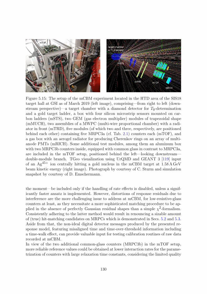
Figure 5.15: The setup of the mCBM experiment located in the HTD area of the SIS18target hall at GSI as of March 2019 (left image), comprising—from right to left (down-stream perspective)—a target chamber with a diamond detector for T0-determinationand a gold target ladder, a box with four silicon microstrip sensors mounted on car-bon ladders (mSTS), two GEM (gas electron multiplier) modules of trapezoidal shape(mMUCH), two assemblies of a MWPC (multi-wire proportional chamber) with a radi-ator in front (mTRD), five modules (of which two and three, respectively, are positionedbehind each other) containing five MRPC3a (cf. Tab. 2.1) counters each (mTOF), anda gas box with an aerogel radiator for producing Cherenkov rings on an array of multi-anode PMTs (mRICH). Some additional test modules, among them an aluminum boxwith two MRPC3b counters inside, equipped with common glass in contrast to MRPC3a,are included in the mTOF setup, positioned behind the left—looking downstream—double-module branch. TGeo visualization using UrQMD and GEANT 3 [119] inputof an Ag45+ ion centrally hitting a gold nucleus in the mCBM target at 1.58 A GeVbeam kinetic energy (right image). Photograph by courtesy of C. Sturm and simulationsnapshot by courtesy of D. Emschermann.

the moment—be included only if the handling of rate effects is disabled, unless a signif-icantly faster ansatz is implemented. However, distortions of response residuals due tointerference are the more challenging issue to address at mCBM, for low-resistive-glasscounters at least, as they necessitate a more sophisticated matching procedure to be ap-plied in the absence of perfectly Gaussian residual shapes than a simple χ2-formalism.Consistently adhering to the latter method would result in renouncing a sizable amountof (true) hit-matching candidates on MRPCs which is demonstrated in Secs. 5.2 and 5.3.Aside from that, the non-ideal digital detector messages produced by the presented re-sponse model, featuring misaligned time and time-over-threshold information includinga time-walk effect, can provide valuable input for testing calibration routines of raw datarecorded at mCBM.In view of the two additional common-glass counters (MRPC3b) in the mTOF setup,more reliable reference values could be obtained at lower interaction rates for the parame-trization of counters with large relaxation time constants, considering the limited quality

130

of data measured with prototype 7-0-0 at CERN/SPS. In contrast to delicate experi-mental conditions at the latter accelerator in March 2015, spill structures at GSI/SIS18during commissioning of mCBM were found to be free of intensity spikes and otherconfounding factors which would bias the performance evaluation of these counters.

131

132

CHAPTER 6

SUMMARY

Multi-gap resistive plate chambers (MRPCs) are a cost-effective solution for large-areatime-of-flight (TOF) measurements in modern nuclear and particle physics experiments,combining excellent timing performance with a high detection efficiency. The 120 m2

TOF wall to be constructed for the Compressed Baryonic Matter (CBM) experiment atthe future FAIR facility is composed of more than 1000 single MRPC detectors varyingin size and in design, depending on anticipated particle fluxes at the respective counterlocation. Experimental conditions in the fixed-target setup of CBM are extreme, giventhe unprecedented beam–target interaction rate of 10 MHz for studying rare probes ingold-on-gold collisions at beam kinetic energies of up to 11 A GeV which corresponds tothe upper limit of the available SIS100 energy range for these projectiles. Closer to thebeam axis, counters are exposed to higher fluxes, approaching 25 kHz/cm2, and trackdensities than at the periphery of the wall which is reflected by a lower resistivity ρ ofthe eponymous glass plates and a finer granularity of readout cells. Local breakdownsof the electric field in the gas gaps upon avalanche formation by traversing chargedparticles deteriorate the detector response function and are recovered on a relaxationtime scale proportional to ρ. Smaller readout cells reduce the probability for signalsinduced by several incident tracks to interfere and generate a distorted counter responsewhich complicates cluster matching between different stations in a tracking setup. Thedouble burden of rate and multi-hit effects on counter performance and on its evaluationin a heavy-ion-collision scenario with high average multiplicities of reaction secondarieswas systematically investigated both in experimental and in simulated data for the firsttime in this work.

Data acquisition/calibration and Monte Carlo studies for test beams

Two MRPC prototypes for the outer TOF wall, the former equipped with low-resistiveglass and the latter built with common glass to study differences in response behavior,were tested at CERN/SPS in March 2015 with collision products of a 19 A GeV/c argonbeam impinging on a lead target. According to a detailed Monte Carlo estimate basedon rates measured with plastic scintillators, mean particle fluxes on the counter surfacesamounted to 1.5 and 1.3 kHz/cm2, respectively, while 3.5 and 3.9 external tracks—on average—passed through the active detection volumes in collision events selectedby coincident hits in a pair of reference counters. These conditions are ideal for thepurpose of this work, allowing for both rate and multi-hit aspects to be studied in ascenario which does not overstrain a common-glass detector in terms of irradiation. Thedata acquisition (DAQ) system based on a network of time-to-digital converters (TDCs)implemented on field-programmable gate arrays (FPGAs) which organized the readoutof 512 electronics channels in the setup was configured and successfully operated as part

133

of this thesis project. In a reduced version, it is still in use for quality control (QC)of mass-produced final counter designs with cosmic rays, as are associated algorithmsfor calibrating and synchronizing TDC raw data. Regarding the free-streaming readoutconcept of CBM which comprises a self-triggered transport of detector raw data from thefront-end electronics to a computing farm for online event reconstruction and selection,not involving a central controller or a hardware trigger derived from coincidences ofdetector signals, a dual readout strategy was embarked on. In addition to a conventionaloperation of the TrbNet communication protocol between a Central Trigger System andTDC nodes with the mentioned physics trigger, a continuous readout of front-end buffers,i.e. a free-streaming mockup, was realized by arranging data transport with a periodicalpulser signal. Thus, samples of time-sorted detector messages could be recorded lackingassociation with a physical event to be retrieved in software by identifying accumulationsof raw data in time. Results obtained for these data sets closely resemble the output ofhardware-triggered runs which—for statistical reasons—were considered for comparisonwith simulated data. However, the handling of mockup data provided valuable guidancefor the subsequent development of time-based algorithms.

Time-based response simulations featuring rate and multi-hit effects

To understand experimental observations concerning detector behavior under rate andmulti-hit load, a reproduction of corresponding effects in simulations is required. Priorto the present work, this functionality did not exist. The transition of the digitizationsoftware for the TOF subsystem within the CbmRoot framework from an event-basedapproach treating single collisions as isolated entities to a time-based scenario allowingfor a continuing impact of occurrences on counters across event borders was accompa-nied by the introduction of a novel parametrization for the detector response function ofMRPCs. The latter can be regarded the main focus of this work. Starting from a set offunctions with adjustable parameters to describe signal induction on readout cells anddiscrimination/digitization jitter in connected readout channels, a response model wasdeveloped which realistically reproduces measured distributions of observables like clus-ter size and time over threshold (ToT), generates non-ideal detector raw data (“digis”)with misaligned timing and ToT information, and intrinsically features an amplitude-dependent time-walk effect. Model parameters for individual counter geometries aredetermined by numerical minimization respecting a number of measured constraints.Degradation effects on counter performance are a direct consequence of the inherentpossibility to downscale the induced charge spectrum which is the basis of responsesampling for an incident particle. A smaller mean charge content of induced signals re-sults in lower amplitudes which less frequently exceed discrimination threshold, reducingdetection efficiency and mean cluster size, and which are subject to a larger discrimi-nation uncertainty of leading and trailing edges, deteriorating the timing response. Tomimic in software the local breakdown and recovery of the electric field in the gas gaps,i.e. the physical mechanism responsible for rate effects, it therefore seemed natural tointroduce a dynamic scaling factor to the random variable representing total induced

134

charge, reflecting the impact of previous particles traversing the counter on the responsefunction of the current one. Individual contributions of tracks stored in this particlememory to the charge coefficient calculated for the most recent passage through theactive detector volume depend on dissipation of the originally induced charge given theelapsed simulation time and on spatial distance between hits on the counter surface. Theinfluence of preceding tracks in time decreases exponentially on an adjustable relaxationtime scale which is typical for the modeled prototype. For qualitative demonstrationpurposes, values of 100 ms for low-resistive-glass MRPCs and of 5 s for common-glasscounters are used in simulations. Concerning interference of signals induced on the samereadout cell by several tracks in a multi-hit environment, consecutive digital detectormessages in an electronics channel are merged if ToT ranges—on the continuous sim-ulation time axis—overlap, causing loss of timing, i.e. leading-edge information of thesubsequent digi and compromising the correction of time walk in the remaining timestamp due to an artificially increased ToT measurement. The latter digi might also bedropped completely if ToT intervals are detached but the TDC channel is still busywith processing the former object within an adjustable dead time. Residual distribu-tions in the two spatial (x and y) and the temporal (t) response dimensions are distortedaccordingly, deviating significantly from the ideal reference of a Gaussian shape. Thiscomplicates the matching of correlated response clusters on different counters whichmeasure traversals of the same particle because the chi-square matching method, forinstance, assumes residuals to be normally distributed.Owing to the quadratic time complexity of the memory algorithm which repeatedly sumsup the respective impact of previously digitized tracks on the current response-samplingprocess, the multithreaded and parallel computing infrastructure provided by the Kro-nos cluster at GSI was exploited to reduce execution times of full-featured test-beamsimulations including rate effects to a manageable level. Within a contiguous memoryperiod which is determined by the length of an accelerator spill (about 10 s during thecampaign at CERN/SPS), the summation load is shared among a configurable numberof threads assigned to computing in parallel partial sums which form the final memorycoefficient. Assuming the break between subsequent spills to be sufficiently long for acomplete recovery of the detector response function, multiple spills are simulated ondifferent computing nodes simultaneously. Due to the dramatic gain in performanceachieved with these measures, a maximum capacity of 30 million memory entries, con-sidering a one-week run-time limitation for jobs on Kronos, allows for a sustained ten-second irradiation of a single large-area MRPC prototype with particle fluxes of up to3.5 kHz/cm2. In simulated heavy-ion collisions in contrast to an illumination scenariowith single muons, however, the limit is slightly more restrictive owing to the creationof secondary tracks in the material budget of detectors which are stored in the memoryin addition to external tracks that are counted towards rate. Regarding the moderateparticle fluxes counters were exposed to at CERN/SPS, a reproduction of test-beamconditions in response simulations is technically feasible, unlike an extrapolation to theentire TOF wall in high-rate simulations of the full CBM setup at nominal irradiationconstraints. For the latter, a segmentation of the counter surface into small independentmemory cells could be an option if edge effects are properly handled.

135

New insights gained from a comparative chi-square analysis

Experimental and simulated results obtained for both types of MRPCs under test, a low-resistive- and a common-glass prototype, were compared in a final analysis based on aχ2-formalism for event selection and matching of correlations on adjacent counters. Realdata had already been associated with events by a physics-triggered data acquisition andsimulated digis residing in timeslice containers of fixed length were grouped into eventsutilizing backlink information on original event affiliations. For performance evaluation,a subset of events with clean matching conditions is chosen, enforced by a χ2-cut of 2.5 onweighted response residuals in time and space between clusters on two selector counters,one of them positioned in front of and the other one installed behind detectors under test(DUT). The response cluster on the rear counter which yields the best selector matchin a given event, identified by the lowest χ2-value, provides an interpolated referencemeasurement for the respective DUT. Here, an additional sorting of residual chi-squaresin ascending order determines the nearest-neighbor (NN) cluster match—in position andtime—between DUT and reference counter. Resolutions in x, y, and t are derived fromGaussian peak fits to NN residual distributions while the detection efficiency is extrap-olated from the integral share of the corresponding χ2-distribution at a limit of 5.0.The applied chi-square matching method does not allow for a comprehensive descriptionof counter performance as residuals in the three response dimensions intrinsically differfrom normal distributions particularly in the tails and deviations increase in a multi-hitenvironment due to signal interference. However, the method proved useful to monitorvariations in detector behavior which were studied systematically as functions of bothhit multiplicity in the setup and irradiation time in spill.Concerning the real prototype equipped with low-resistive glass, the χ2-efficiency isfound to improve by more than 7 % in absolute numbers from an estimate of 77.2 % with-out any cut on multiplicity to a value of 84.5 % if only a single cluster is generated on thefirst selector counter in the respective event. In the same time, the general availabilityof any cluster on the DUT, i.e. the NN acceptance, decreases from 98.6 % to 94.4 % ofselector events. This numerical example of a counter which did not generate a (recorded)response for every incident particle is illustrative for the growing impact of mismatchesand residual distortions—due to interfering signals—on the detector response functionunder increasing multi-hit conditions. The remaining discrepancy between acceptanceand χ2-efficiency at the strictest multiplicity cut indicates the limited applicability of arigorous chi-square formalism to cluster matching between MRPCs. Within this work,light was shed on this difficulty for the first time in a methodical way. Analogous trends,albeit less pronounced, are observed for position and time resolutions owing to narrow-ing residual centers in the absence of the former influences. Even without restricting theanalyzed event sample to cases of low hit multiplicities, Gaussian residual peak widthsof 0.5 cm in x and y and of 65 ps in t are achieved with this detector, still including acontribution from the reference counter. Hence, compliance with the required systemtime resolution of 80 ps for CBM TOF is given.With progressing time in spill, response observables evaluated for this prototype do notshow any sign of deterioration, as expected for low-resistive glass under these moderate

136

particle fluxes. Experimental results for the common-glass detector, in contrast, clearlyreflect a susceptibility of the counter design to rate effects at fluxes around 1 kHz/cm2,comprising—besides efficiency—mean cluster size, mean time over threshold, and res-olutions. These findings are the first evidence of in-spill response degradation of anMRPC observed in a heavy-ion-collision scenario. However, a time average obtained forthe χ2-efficiency of only 32.2 % implies biased starting conditions for performance eval-uation caused by a spike in beam intensity which preceded every spill at CERN/SPS.Consequently, the detector is relatively prone to NN mismatches, given the large activearea as compared to the selection zone, which add significant background to residualdistributions and broaden residual peaks. The resulting poor resolutions without a cuton multiplicity considerably improve towards a single-cluster constraint.Qualitatively, the behavior of both real prototypes was reproduced with the responsemodel developed in this work, using different relaxation parameters for the two typesof glass in a pioneering rate simulation of a full test-beam setup. Known limitationsexist concerning the overlarge width of local y-residuals in simulations and a restric-tion to the efficiency range ε > 50 % below which counterintuitive trend reversals occurin virtual response observables. A quantitative agreement as such with individual re-sults obtained for detectors under test at CERN/SPS was not primarily aimed at whenadjusting model parameters for various counter geometries with an identical set of min-imization constraints. However, it can be achieved upon redetermination of parametervalues according to a particular case.

Outlook

The interplay of rate and multi-hit effects on MRPC performance in high-intensityheavy-ion-collision experiments is a pending problem to be addressed by the CBM-TOF working group in the years ahead towards completion of the FAIR facility in 2025.This work represents a first systematic investigation of the consequences of correspond-ing experimental conditions for the detector response function and for hit matchingbetween counters. An application and further development of the implemented digiti-zation software featuring a parametrization of both degradation aspects at the runningmCBM experiment is intended. Pursuing an inadequate χ2-matching strategy in view ofresponse residuals which increasingly deviate from normal distributions the more likelyinduced signals are to interfere on a readout cell is a source of efficiency loss and requiresremedial action. This refinement process of matching methods needs to be accompaniedby simulations which reproduce observed behavior and provide information on matchingpurity. The presented response model is a suitable tool for this task.

137

138

APPENDICES

139

140

APPENDIX A

CURRICULUM VITAE

Personal Information

Name Christian Helmut Simon

Gender male

Date of birth 15/08/1987

Place of birth Wiesbaden, Germany

Marital status single

Citizenship German

Education

03/2012 – present Doctoral studies in physics at Heidelberg University, Germany

09/2011 – 02/2012 Master studies in physics at Heidelberg University, Germany

08/2011 Master of Science in physics

08/2010 – 08/2011 Master studies in physics at Michigan State University, USA

07/2010 Bachelor of Science in physics

09/2007 – 07/2010 Bachelor studies in physics at Heidelberg University, Germany

06/2007 Allgemeine Hochschulreife(general university entrance qualification)

09/1998 – 06/2007 Furst-Johann-Ludwig-Schule in Hadamar, Germany(gymnasium)

08/1994 – 07/1998 Primary school in Dornburg-Thalheim, Germany

Scholarships

04/2012 – 12/2015 Helmholtz Graduate School for Hadron and Ion Research(HGS-HIRe for FAIR)

10/2007 – 03/2012 Studienstiftung des deutschen Volkes(German Academic Scholarship Foundation)

Heidelberg, November 30, 2020

141

142

APPENDIX B

LIST OF PUBLICATIONS

Refereed Journal Papers

M. Petris, D. Bartos, M. Petrovici, L. Radulescu, V. Simion, J. Fruhauf, M. Kis, P.-A.Loizeau, I. Deppner, N. Herrmann, and C. Simon, “Performance of a two-dimensionalposition sensitive MRPC prototype with adjustable transmission line impedance,” Nucl.Instrum. Meth. A 920, 100 (2019).

T. Ablyazimov et al. (CBM Collaboration), “Challenges in QCD matter physics – Thescientific programme of the Compressed Baryonic Matter experiment at FAIR,” Eur.Phys. J. A 53, 60 (2017), arXiv:1607.01487 [nucl-ex].

C. H. Simon and P. Danielewicz, “Interplay of anisotropies of momentum distributionand mean field in heavy-ion collisions,” Phys. Rev. C 87, 054619 (2013), arXiv:1212.4460[nucl-th].

Refereed Conference Papers

P. Lyu, D. Han, Y. Wang, Q. Zhang, B. Guo, F. Wang, Y. Yu, X. Chen, Y. Li, N. Herr-mann, I. Deppner, C. Simon, P. Weidenkaff, P.-A. Loizeau, and J. Fruhauf, “Studyon cosmic test and QC method of high-rate MRPC for CBM-TOF,” Proceedings, 14thWorkshop on Resistive Plate Chambers and Related Detectors (RPC2018): Puerto Val-larta, Jalisco state, Mexico, February 19–23, 2018, J. Instrum. 14, C09032 (2019).

M. Petris, D. Bartos, M. Petrovici, L. Radulescu, V. Simion, J. Frunhauf, P.-A. Loizeau,I. Deppner, N. Herrmann, and C. Simon, “Performance tests of the MSMGRPCs usinga free-streaming readout,” Proceedings, 39th International Conference on High EnergyPhysics (ICHEP2018): Seoul, Korea, July 4–11, 2018, Proc. Sci. 340, 663 (2019).

D. Hu, D. Sauter, X. Wang, Y. Sun, I. Deppner, N. Herrmann, C. Simon, Ph. Weidenkaff,J. Brandt, J. Zhou, M. Shao, C. Li, H. Chen, Z. Tang, Y. Zhang, E. Lavrik, andH. Zeng, “MRPC3b mass production for CBM-TOF and eTOF at STAR,” Proceedings,14th Workshop on Resistive Plate Chambers and Related Detectors (RPC2018): PuertoVallarta, Jalisco state, Mexico, February 19–23, 2018, J. Instrum. 14, C06013 (2019),arXiv:1807.02452 [physics.ins-det].

M. Petris, D. Bartos, M. Petrovici, L. Radulescu, V. Simion, I. Deppner, N. Herrmann,C. Simon, J. Fruhauf, M. Kis, and P-A. Loizeau, “In-beam test of the RPC architec-ture foreseen to be used for the CBM-TOF inner wall,” Proceedings, 22nd InternationalSchool on Nuclear Physics, Neutron Physics and Applications: Varna, Bulgaria, Septem-ber 10–16, 2017, J. Phys. Conf. Ser. 1023, 012007 (2018).

C. Simon, I. Deppner, and N. Herrmann (for the CBM Collaboration), “The physicsprogram of the CBM experiment,” Proceedings, 11th International Workshop on Critical

143

Point and Onset of Deconfinement (CPOD2017): Stony Brook, New York, USA, August7–11, 2017, Proc. Sci. 311, 014 (2018).

P. Lyu, Y. Wang, B. Guo, D. Han, Y. Li, N. Herrmann, I. Deppner, C. Simon, P. Wei-denkaff, F. Jochen, P.-A. Loizeau, and M. Laden Kis, “Development and performanceof self-sealed MRPC,” Proceedings, 14th Topical Seminar on Innovative Particle andRadiation Detectors (IPRD16): Siena, Italy, October 3–6, 2016, J. Instrum. 12, C03055(2017).

Y. Wang, X. J. Huang, P. F. Lyu, D. Han, B. Xie, Y. J. Li, N. Herrmann, I. Deppner,P. Loizeau, C. Simon, J. Fruhauf, and M. Kis, “A solution for the inner area of CBM-TOF with pad-MRPC,” Proceedings, 14th Vienna Conference on Instrumentation (VCI2016): Vienna, Austria, February 15–19, 2016, Nucl. Instrum. Meth. A 845, 318 (2017).

I. Deppner, N. Herrmann, J. Fruhauf, M. Kis, P. Lyu, P.-A. Loizeau, L. Shi, C. Simon,Y. Wang, and B. Xie, “Performance studies of MRPC prototypes for CBM,” Proceed-ings, 13th Workshop on Resistive Plate Chambers and Related Detectors (RPC2016):Ghent, Belgium, February 22–26, 2016, J. Instrum. 11, C10006 (2016), arXiv:1606.04917[physics.ins-det].

M. Petris, D. Bartos, G. Caragheorgheopol, I. Deppner, J. Fruhauf, N. Herrmann,M. Kis, P.-A. Loizeau, M. Petrovici, L. Radulescu, V. Simion, and C. Simon, “Timeand position resolution of high granularity, high counting rate MRPC for the inner zoneof the CBM-TOF wall,” Proceedings, 13th Workshop on Resistive Plate Chambers andRelated Detectors (RPC2016): Ghent, Belgium, February 22–26, 2016, J. Instrum. 11,C09009 (2016), arXiv:1605.02558 [physics.ins-det].

Y. Wang, P. Lyu, X. Huang, D. Han, B. Xie, Y. Li, N. Herrmann, I. Deppner, C. Simon,P.-A. Loizeau, P. Weidenkaff, J. Fruhauf, and M. Laden Kis, “Development and testof a real-size MRPC for CBM-TOF,” Proceedings, 13th Workshop on Resistive PlateChambers and Related Detectors (RPC2016): Ghent, Belgium, February 22–26, 2016,J. Instrum. 11, C08007 (2016), arXiv:1605.02395 [physics.ins-det].

M. Petris, D. Bartos, G. Caragheorgheopol, F. Constantin, M. Petrovici, L. Radulescu,V. Simion, I. Deppner, N. Herrmann, C. Simon, J. Fruhauf, M. Kis, and P-A. Loizeau,“Prototype with the basic architecture for the CBM-TOF inner wall tested in close toreal conditions,” Proceedings, 21st International School on Nuclear Physics, NeutronPhysics and Applications & International Symposium on Exotic Nuclei (ISEN-2015):Varna, Bulgaria, September 7–12, 2015, J. Phys. Conf. Ser. 724, 012037 (2016).

I. Deppner, N. Herrmann, A. Akindinov, D. Bartos, A. Balaceanu, S. Belogurov,P. Cao, G. Caragheorgheopol, H. Chen, J. Cheng, M. Ciobanu, F. Constantin, Z. Deng,H. Deppe, V. Duta, H. Fan, H. Flemming, J. Fruhauf, J. Gebelein, K. Heidel, K. Hilden-brand, U. Kebschull, M. Kis, S. Kiselev, K. Koch, P. Koczon, R. Kotte, A. Laso Gar-cia, J. Lehrbach, C. Li, Y. Li, P.-A. Loizeau, P. Lv, D. Malkevich, S. Manz, L. Nau-mann, A. Nedosekin, W. Niebur, A. Oancea, M. Petris, M. Petrovici, V. Plotnikov,M. Prokudin, L. Radulescu, M. Shao, V. Simion, C. Simon, R. Sultanov, Y. Sun, Z. Tang,

144

Y. Wang, J. Wustenfeld, C. Xiang, N. Xu, Y. Zhang, D. Zhou, and X. Zhu, “The CBMTime-of-Flight wall — a conceptual design,” Proceedings, 12th Workshop on ResistivePlate Chambers and Related Detectors (RPC2014): Beijing, China, February 23–28,2014, J. Instrum. 9, C10014 (2014).

C. Simon, I. Deppner, N. Herrmann, P.-A. Loizeau, and J. Fruhauf, “Performancetest of a fully differential float-glass multi-strip MRPC prototype for the CBM ToFwall with cosmic rays,” Proceedings, 12th Workshop on Resistive Plate Chambers andRelated Detectors (RPC2014): Beijing, China, February 23–28, 2014, J. Instrum. 9,C09028 (2014).

Master’s Thesis

C. H. Simon, Interplay of anisotropy of momentum distributions and mean fields inheavy-ion collisions , Michigan State University, East Lansing, Michigan, USA (2011).

Bachelor’s Thesis

C. Simon, An acceptance study of charged K mesons in the SIS-100 energy range for theCBM ToF wall, Heidelberg University, Heidelberg, Germany (2010).

145

146

REFERENCES

147

148

REFERENCES

[1] S. Klimt, M. Lutz, and W. Weise, “Chiral phase transition in the SU(3) Nambuand Jona-Lasinio model,” Phys. Lett. B 249, 386 (1990).

[2] D. H. Rischke, “The quark–gluon plasma in equilibrium,” Prog. Part. Nucl. Phys.52, 197 (2004), arXiv:nucl-th/0305030.

[3] L. McLerran and R. D. Pisarski, “Phases of dense quarks at large Nc,” Nucl. Phys.A 796, 83 (2007), arXiv:0706.2191 [hep-ph].

[4] M. G. Alford, A. Schmitt, K. Rajagopal, and T. Schafer, “Color superconductivityin dense quark matter,” Rev. Mod. Phys. 80, 1455 (2008), arXiv:0709.4635 [hep-ph].

[5] K. Fukushima and T. Hatsuda, “The phase diagram of dense QCD,” Rep. Prog.Phys. 74, 014001 (2011), arXiv:1005.4814 [hep-ph].

[6] K. Aamodt et al. (ALICE Collaboration), “The ALICE experiment at the CERNLHC,” J. Instrum. 3, S08002 (2008).

[7] J. Adams et al. (STAR Collaboration), “Experimental and theoretical challengesin the search for the quark–gluon plasma: The STAR Collaboration’s critical as-sessment of the evidence from RHIC collisions,” Nucl. Phys. A 757, 102 (2005),arXiv:nucl-ex/0501009.

[8] J. M. Lattimer and M. Prakash, “The Physics of Neutron Stars,” Science 304, 536(2004), arXiv:astro-ph/0405262.

[9] H. H. Gutbrod et al., eds., FAIR Baseline Technical Report (GSI, Darmstadt,Germany, 2006).

[10] CBM Collaboration, Compressed Baryonic Matter Experiment — Technical StatusReport (GSI, Darmstadt, Germany, 2005).

[11] P. Braun-Munzinger, K. Redlich, and J. Stachel, “Particle Production in HeavyIon Collisions,” in Quark–Gluon Plasma 3 , edited by R. C. Hwa and X.-N. Wang(World Scientific, Singapore, 2004) p. 491, arXiv:nucl-th/0304013.

[12] A. Andronic, P. Braun-Munzinger, and J. Stachel, “The horn, the hadron massspectrum and the QCD phase diagram – the statistical model of hadron productionin central nucleus-nucleus collisions,” Proceedings, 10th International Conferenceon Nucleus-Nucleus Collisions (NN2009): Beijing, China, August 16–21, 2009,Nucl. Phys. A 834, 237c (2010), arXiv:0911.4931 [nucl-th].

149

[13] F. Li, L.-W. Chen, C. M. Ko, and S. H. Lee, “Contributions of hyperon-hyperonscattering to subthreshold cascade production in heavy ion collisions,” Phys. Rev.C 85, 064902 (2012), arXiv:1204.1327 [nucl-th].

[14] G. Agakishiev et al. (HADES Collaboration), “Statistical hadronization modelanalysis of hadron yields in p + Nb and Ar + KCl at SIS18 energies,” Eur. Phys.J. A 52, 178 (2016), arXiv:1512.07070 [nucl-ex].

[15] S. Wheaton, J. Cleymans, and M. Hauer, “THERMUS—A thermal model packagefor ROOT,” Comput. Phys. Commun. 180, 84 (2009), arXiv:hep-ph/0407174.

[16] C. Alt et al. (NA49 Collaboration), “Pion and kaon production in central Pb + Pbcollisions at 20A and 30A GeV: Evidence for the onset of deconfinement,” Phys.Rev. C 77, 024903 (2008), arXiv:0710.0118 [nucl-ex].

[17] A. Palmese, W. Cassing, E. Seifert, T. Steinert, P. Moreau, and E. L.Bratkovskaya, “Chiral symmetry restoration in heavy-ion collisions at interme-diate energies,” Phys. Rev. C 94, 044912 (2016), arXiv:1607.04073 [nucl-th].

[18] W. Cassing and E. L. Bratkovskaya, “Parton transport and hadronization fromthe dynamical quasiparticle point of view,” Phys. Rev. C 78, 034919 (2008),arXiv:0808.0022 [hep-ph].

[19] W. Cassing and E. L. Bratkovskaya, “Parton–hadron–string dynamics: An off-shell transport approach for relativistic energies,” Nucl. Phys. A 831, 215 (2009),arXiv:0907.5331 [nucl-th].

[20] C. Blume, “Energy dependence of hadronic observables,” Proceedings, Workshopfor Young Scientists on the Physics of Ultrarelativistic Nucleus–Nucleus Collisions(Hot Quarks 2004): Taos Valley, New Mexico, USA, July 18–24, 2004, J. Phys.G 31, S57 (2005).

[21] C. Simon, I. Deppner, and N. Herrmann (for the CBM Collaboration), “Thephysics program of the CBM experiment,” Proceedings, 11th International Work-shop on Critical Point and Onset of Deconfinement (CPOD2017): Stony Brook,New York, USA, August 7–11, 2017, Proc. Sci. 311, 014 (2018).

[22] V. Friese (for the CBM Collaboration), “Strangeness Prospects with the CBMExperiment,” Proceedings, 15th International Conference on Strangeness in QuarkMatter (SQM-2015): Dubna, Russia, July 6–11, 2015, J. Phys. Conf. Ser. 668,012014 (2016).

[23] V. Khachatryan et al. (CMS Collaboration), “Measurement of the transverse mo-mentum spectrum of the Higgs boson produced in pp collisions at

√s = 8 TeV

using H→WW decays,” J. High Energy Phys. 03, 032 (2017), arXiv:1606.01522[hep-ex].

150

[24] J. K. Ahn et al. (E373 (KEK-PS) Collaboration), “Double-Λ hypernuclei observedin a hybrid emulsion experiment,” Phys. Rev. C 88, 014003 (2013).

[25] S.-I. Maeda, Y. Akaishi, and T. Yamazaki, “K−K−pp - an important gatewaytoward multi-kaonic nuclei,” Proceedings, 12th International Conference on Hy-pernuclear and Strange Particle Physics (HYP2015): Sendai, Japan, September7–12, 2015, JPS Conf. Proc. 17, 082007 (2017), arXiv:1610.02150 [nucl-ex].

[26] T. Yamazaki, A. Dote, and Y. Akaishi, “Invariant-mass spectroscopy for con-densed single- and double-K nuclear clusters to be formed as residues in relativisticheavy-ion collisions,” Phys. Lett. B 587, 167 (2004), arXiv:nucl-th/0310085.

[27] A. Andronic, P. Braun-Munzinger, J. Stachel, and H. Stocker, “Production oflight nuclei, hypernuclei and their antiparticles in relativistic nuclear collisions,”Phys. Lett. B 697, 203 (2011), arXiv:1010.2995 [nucl-th].

[28] A. Andronic, P. Braun-Munzinger, and K. Redlich, “Statistical production ofantikaon nuclear bound states in heavy ion collisions,” Nucl. Phys. A 765, 211(2006), arXiv:nucl-th/0506083.

[29] P. A. Zyla et al. (Particle Data Group), “Review of Particle Physics,” Prog. Theor.Exp. Phys. 2020, 083C01 (2020).

[30] I. Vassiliev, private communication (2017).

[31] T. Ablyazimov et al. (CBM Collaboration), “Challenges in QCD matter physics– The scientific programme of the Compressed Baryonic Matter experiment atFAIR,” Eur. Phys. J. A 53, 60 (2017), arXiv:1607.01487 [nucl-ex].

[32] I. Deppner, private communication (2020).

[33] I. Deppner et al., “The CBM time-of-flight wall,” Proceedings, 10th Workshopon Resistive Plate Chambers and Related Detectors (RPC2010): Darmstadt, Ger-many, February 9–12, 2010, Nucl. Instrum. Meth. A 661, S121 (2012).

[34] C. Simon, I. Deppner, N. Herrmann, P.-A. Loizeau, and J. Fruhauf, “Performancetest of a fully differential float-glass multi-strip MRPC prototype for the CBM ToFwall with cosmic rays,” Proceedings, 12th Workshop on Resistive Plate Chambersand Related Detectors (RPC2014): Beijing, China, February 23–28, 2014, J. In-strum. 9, C09028 (2014).

[35] CBM Collaboration, mCBM@SIS18 — A CBM full system test-setup for high-ratenucleus-nucleus collisions at GSI / FAIR (GSI, Darmstadt, Germany, 2017).

[36] B. Friman et al., eds., The CBM Physics Book , Lect. Notes Phys. 814 (Springer,Berlin/Heidelberg, Germany, 2011).

151

[37] P. Kurilkin et al., “Superconducting dipole magnet for the CBM experiment atFAIR,” Proceedings, 23rd International Baldin Seminar on High Energy PhysicsProblems: Relativistic Nuclear Physics & Quantum Chromodynamics (BaldinISHEPP XXIII): Dubna, Russia, September 19–24, 2016, EPJ Web Conf. 138,12001 (2017).

[38] CBM Collaboration, Technical Design Report for the CBM Superconducting DipoleMagnet, edited by A. Malakhov and A. Shabunov (GSI, Darmstadt, Germany,2013).

[39] M. Koziel et al., “Vacuum-compatible, ultra-low material budget Micro-Vertex De-tector of the compressed baryonic matter experiment at FAIR,” Proceedings, 14thVienna Conference on Instrumentation (VCI 2016): Vienna, Austria, February15–19, 2016, Nucl. Instrum. Meth. A 845, 110 (2017).

[40] J. M. Heuser, “The Silicon Tracking System of the CBM Experiment at FAIR,”Proceedings, 2nd International Symposium on Science at J-PARC: Unlocking theMysteries of Life, Matter and the Universe (J-PARC 2014): Tsukuba, Japan, July12–15, 2014, JPS Conf. Proc. 8, 022007 (2015).

[41] CBM Collaboration, Technical Design Report for the CBM Silicon Tracking System(STS), edited by J. Heuser et al. (GSI, Darmstadt, Germany, 2013).

[42] J. Adamczewski-Musch et al., “The CBM RICH project,” Proceedings, 14th Vi-enna Conference on Instrumentation (VCI 2016): Vienna, Austria, February 15–19, 2016, Nucl. Instrum. Meth. A 845, 434 (2017).

[43] CBM Collaboration, Technical Design Report for the CBM Ring ImagingCherenkov (RICH) Detector, edited by C. Hohne (GSI, Darmstadt, Germany,2013).

[44] A. K. Dubey et al., “GEM based R&D for muon chambers of CBM experimentat FAIR,” Proceedings, 3rd International Conference on Micro Pattern GaseousDetectors (MPGD2013): Zaragoza, Spain, July 1–4, 2013, J. Instrum. 9, C06004(2014).

[45] CBM Collaboration, Technical Design Report for the CBM Muon Chambers(MuCh), edited by S. Chattopadhyay, Y. P. Viyogi, P. Senger, W. F. J. Muller,and C. J. Schmidt (GSI, Darmstadt, Germany, 2015).

[46] P. Kahler and F. Roether (for the CBM Collaboration), “The transition radiationdetector in the CBM experiment at FAIR,” Proceedings, 15th Vienna Conferenceon Instrumentation (VCI 2019): Vienna, Austria, February 18–22, 2019, Nucl.Instrum. Meth. A 958, 162727 (2020).

[47] CBM Collaboration, Technical Design Report for the CBM Transition RadiationDetector (TRD), edited by C. Blume, C. Bergmann, and D. Emschermann (GSI,Darmstadt, Germany, 2018).

152

[48] I. Deppner et al., “The CBM Time-of-Flight wall — a conceptual design,” Pro-ceedings, 12th Workshop on Resistive Plate Chambers and Related Detectors(RPC2014): Beijing, China, February 23–28, 2014, J. Instrum. 9, C10014 (2014).

[49] CBM Collaboration, Technical Design Report for the CBM Time-of-Flight System(TOF), edited by N. Herrmann (GSI, Darmstadt, Germany, 2014).

[50] I. E. Korolko, M. S. Prokudin, and Y. M. Zaitsev, “The CBM ECAL,” Proceedings,2nd International Conference on Particle Physics and Astrophysics (ICPPA-2016):Moscow, Russia, October 10–14, 2016, J. Phys. Conf. Ser. 798, 012164 (2017).

[51] V. Klochkov and I. Selyuzhenkov (for the CBM Collaboration), “Centrality de-termination in heavy-ion collisions with the CBM experiment,” Proceedings, 2ndInternational Conference on Particle Physics and Astrophysics (ICPPA-2016):Moscow, Russia, October 10–14, 2016, J. Phys. Conf. Ser. 798, 012059 (2017).

[52] CBM Collaboration, Technical Design Report for the CBM Projectile Spectator De-tector (PSD), edited by F. Guber and I. Selyuzhenkov (GSI, Darmstadt, Germany,2015).

[53] J. de Cuveland and V. Lindenstruth (for the CBM Collaboration), “A First-levelEvent Selector for the CBM Experiment at FAIR,” Proceedings, 18th InternationalConference on Computing in High Energy and Nuclear Physics (CHEP 2010):Taipei, Taiwan, October 18–22, 2010, J. Phys. Conf. Ser. 331, 022006 (2011).

[54] W. M. Zabo lotny et al., “Selection of hardware platform for CBM Common Read-out Interface,” Proceedings, 40th Wilga Symposium on Photonics Applications inAstronomy, Communications, Industry, and High-Energy Physics Experiments:Wilga, Poland, May 29 – June 4, 2017, Proc. SPIE 10445, 1044549 (2017).

[55] J. Lehnert et al., “GBT based readout in the CBM experiment,” Proceedings,Topical Workshop on Electronics for Particle Physics (TWEPP 2016): Karlsruhe,Germany, September 26–30, 2016, J. Instrum. 12, C02061 (2017).

[56] L. Meder, J. Lebedev, and J. Becker, “A versatile small form factor twisted-pairTFC FMC for MTCA AMCs,” Proceedings, Topical Workshop on Electronics forParticle Physics (TWEPP 2016): Karlsruhe, Germany, September 26–30, 2016,J. Instrum. 12, C03074 (2017).

[57] J. de Cuveland, D. Hutter, and V. Lindenstruth, “CBM First-level Event Selec-tor data management developments,” in CBM Progress Report 2013, edited byV. Friese and C. Sturm (GSI, Darmstadt, Germany, 2014) p. 92.

[58] I. Kisel, “Scientific and high-performance computing at FAIR,” Proceedings, 3rdInternational Conference on New Frontiers in Physics (ICNFP 2014): Kolymbari,Crete, Greece, July 28 – August 6, 2014, EPJ Web Conf. 95, 01007 (2015).

153

[59] V. Akishina and I. Kisel, “4-Dimensional Event Building in the First-Level EventSelection of the CBM Experiment,” Proceedings, 21st International Conference onComputing in High Energy and Nuclear Physics (CHEP 2015): Okinawa, Japan,April 13–17, 2015, J. Phys. Conf. Ser. 664, 072027 (2015).

[60] I. E. Korolko, M. S. Prokudin, and Y. M. Zaitsev, “Event building for free-streaming readout in the CBM experiment,” Proceedings, 2nd International Con-ference on Particle Physics and Astrophysics (ICPPA-2016): Moscow, Russia,October 10–14, 2016, J. Phys. Conf. Ser. 798, 012165 (2017).

[61] S. Lebedev, C. Hohne, A. Lebedev, and G. Ososkov, “Selected event reconstruc-tion algorithms for the CBM experiment at FAIR,” Proceedings, 20th InternationalConference on Computing in High Energy and Nuclear Physics (CHEP 2013): Am-sterdam, The Netherlands, October 14–18, 2013, J. Phys. Conf. Ser. 513, 022019(2014).

[62] M. Al-Turany et al., “The FairRoot framework,” Proceedings, 19th InternationalConference on Computing in High Energy and Nuclear Physics (CHEP 2012):New York City, USA, May 21–25, 2012, J. Phys. Conf. Ser. 396, 022001 (2012).

[63] R. Brun and F. Rademakers, “ROOT — An object oriented data analysis frame-work,” Proceedings, 5th International Workshop on New Computing Techniquesin Physics Research (AIHENP’96): Lausanne, Switzerland, September 2–6, 1996,Nucl. Instrum. Meth. A 389, 81 (1997).

[64] V. Friese (for the CBM Collaboration), “The high-rate data challenge: computingfor the CBM experiment,” Proceedings, 22nd International Conference on Com-puting in High Energy and Nuclear Physics (CHEP 2016): San Francisco, USA,October 10–14, 2016, J. Phys. Conf. Ser. 898, 112003 (2017).

[65] S. A. Bass et al., “Microscopic Models for Ultrarelativistic Heavy Ion Collisions,”Prog. Part. Nucl. Phys. 41, 255 (1998), arXiv:nucl-th/9803035.

[66] M. Bleicher et al., “Relativistic hadron–hadron collisions in the ultra-relativisticquantum molecular dynamics model,” J. Phys. G 25, 1859 (1999), arXiv:hep-ph/9909407.

[67] I. Hrivnacova et al. (for the ALICE Collaboration), “The Virtual Monte Carlo,”Proceedings, 13th International Conference on Computing in High Energy andNuclear Physics (CHEP 2003): La Jolla, California, USA, March 24–28, 2003,eConf C0303241, THJT006 (2003), arXiv:cs/0306005 [cs.SE].

[68] R. Brun, A. Gheata, and M. Gheata (for the ALICE Collaboration), “A Geometri-cal Modeller for HEP,” Proceedings, 13th International Conference on Computingin High Energy and Nuclear Physics (CHEP 2003): La Jolla, California, USA,March 24–28, 2003, eConf C0303241, THMT001 (2003), arXiv:physics/0306151[physics.comp-ph].

154

[69] V. Friese, “A cluster-finding algorithm for free-streaming data,” Proceedings, 23rdInternational Conference on Computing in High Energy and Nuclear Physics(CHEP 2018): Sofia, Bulgaria, July 9–13, 2018, EPJ Web Conf. 214, 01008(2019).

[70] M. Al-Turany, D. Klein, A. Manafov, A. Rybalchenko, and F. Uhlig, “Extendingthe FairRoot framework to allow for simulation and reconstruction of free stream-ing data,” Proceedings, 20th International Conference on Computing in High En-ergy and Nuclear Physics (CHEP 2013): Amsterdam, The Netherlands, October14–18, 2013, J. Phys. Conf. Ser. 513, 022001 (2014).

[71] C. Lippmann, “Particle identification,” Nucl. Instrum. Meth. A 666, 148 (2012),arXiv:1101.3276 [hep-ex].

[72] A. Akindinov et al., “Performance of the ALICE Time-Of-Flight detector at theLHC,” Eur. Phys. J. Plus 128, 44 (2013).

[73] E. Cerron Zeballos et al., “A new type of resistive plate chamber: The multigapRPC,” Nucl. Instrum. Meth. A 374, 132 (1996).

[74] W. Riegler, C. Lippmann, and R. Veenhof, “Detector physics and simulation ofresistive plate chambers,” Nucl. Instrum. Meth. A 500, 144 (2003).

[75] M. Abbrescia, “Improving rate capability of Resistive Plate Chambers,” Pro-ceedings, 13th Workshop on Resistive Plate Chambers and Related Detectors(RPC2016): Ghent, Belgium, February 22–26, 2016, J. Instrum. 11, C10001(2016).

[76] M. C. S. Williams, “Particle identification using time of flight,” J. Phys. G 39,123001 (2012).

[77] D. Gonzalez-Diaz et al., “The role of the Resistive Plate response function inbringing an RPC to a stationary situation,” Proceedings, 9th Workshop on Resis-tive Plate Chambers and Related Detectors (RPC2007): Mumbai, India, February13–16, 2008, Nucl. Instrum. Meth. A 602, 713 (2009).

[78] D. Gonzalez-Dıaz, P. Fonte, J. A. Garzon, and A. Mangiarotti, “An analyticaldescription of rate effects in timing RPCs,” Proceedings, 8th Workshop on ResistivePlate Chambers and Related Detectors (RPC2005): Seoul, Korea, October 10–12,2005, Nucl. Phys. B Proc. Suppl. 158, 111 (2006).

[79] J. Wang et al., “Development of multi-gap resistive plate chambers with low-resistive silicate glass electrodes for operation at high particle fluxes and largetransported charges,” Nucl. Instrum. Meth. A 621, 151 (2010).

[80] M. Ciobanu et al., “PADI, an Ultrafast Preamplifier - Discriminator ASIC forTime-of-Flight Measurements,” IEEE Trans. Nucl. Sci. 61, 1015 (2014).

155

[81] H. Deppe and H. Flemming, “The GSI Event-Driven TDC with 4 ChannelsGET4,” Proceedings, 2009 IEEE Nuclear Science Symposium and Medical Imag-ing Conference (NSS/MIC 2009): Orlando, Florida, USA, October 25–31, 2009,IEEE Nucl. Sci. Symp. Conf. Rec. 2009, 295 (2009).

[82] A. Akindinov et al., “Radiation-hard ceramic Resistive Plate Chambers for forwardTOF and T0 systems,” Proceedings, 14th Vienna Conference on Instrumentation(VCI 2016): Vienna, Austria, February 15–19, 2016, Nucl. Instrum. Meth. A 845,203 (2017).

[83] Y. Wang et al., “Development and test of a real-size MRPC for CBM-TOF,”Proceedings, 13th Workshop on Resistive Plate Chambers and Related Detectors(RPC2016): Ghent, Belgium, February 22–26, 2016, J. Instrum. 11, C08007(2016), arXiv:1605.02395 [physics.ins-det].

[84] M. Petris et al., “Time and position resolution of high granularity, high countingrate MRPC for the inner zone of the CBM-TOF wall,” Proceedings, 13th Work-shop on Resistive Plate Chambers and Related Detectors (RPC2016): Ghent, Bel-gium, February 22–26, 2016, J. Instrum. 11, C09009 (2016), arXiv:1605.02558[physics.ins-det].

[85] I. Deppner et al., “Performance studies of MRPC prototypes for CBM,” Pro-ceedings, 13th Workshop on Resistive Plate Chambers and Related Detectors(RPC2016): Ghent, Belgium, February 22–26, 2016, J. Instrum. 11, C10006(2016), arXiv:1606.04917 [physics.ins-det].

[86] Y. Wang et al., “A solution for the inner area of CBM-TOF with pad-MRPC,”Proceedings, 14th Vienna Conference on Instrumentation (VCI 2016): Vienna,Austria, February 15–19, 2016, Nucl. Instrum. Meth. A 845, 318 (2017).

[87] P. Lyu et al., “Development and performance of self-sealed MRPC,” Proceedings,14th Topical Seminar on Innovative Particle and Radiation Detectors (IPRD16):Siena, Italy, October 3–6, 2016, J. Instrum. 12, C03055 (2017).

[88] M. Petris et al., “In-beam test of the RPC architecture foreseen to be used forthe CBM-TOF inner wall,” Proceedings, 22nd International School on NuclearPhysics, Neutron Physics and Applications: Varna, Bulgaria, September 10–16,2017, J. Phys. Conf. Ser. 1023, 012007 (2018).

[89] M. Petris et al., “Performance of a two-dimensional position sensitive MRPC pro-totype with adjustable transmission line impedance,” Nucl. Instrum. Meth. A 920,100 (2019).

[90] A. Neiser et al., “TRB3: a 264 channel high precision TDC platform and itsapplications,” Proceedings, Topical Workshop on Electronics for Particle Physics(TWEPP 2013): Perugia, Italy, September 23–27, 2013, J. Instrum. 8, C12043(2013).

156

[91] P. Lyu et al., “Study on cosmic test and QC method of high-rate MRPC forCBM-TOF,” Proceedings, 14th Workshop on Resistive Plate Chambers and RelatedDetectors (RPC2018): Puerto Vallarta, Jalisco state, Mexico, February 19–23,2018, J. Instrum. 14, C09032 (2019).

[92] D. Hu et al., “MRPC3b mass production for CBM-TOF and eTOF at STAR,”Proceedings, 14th Workshop on Resistive Plate Chambers and Related Detectors(RPC2018): Puerto Vallarta, Jalisco state, Mexico, February 19–23, 2018, J. In-strum. 14, C06013 (2019), arXiv:1807.02452 [physics.ins-det].

[93] STAR Collaboration and CBM Collaboration eTOF Group, “Physics Program forthe STAR/CBM eTOF Upgrade,” arXiv:1609.05102 [nucl-ex].

[94] J. Michel et al., “The HADES DAQ System: Trigger and Readout Board Net-work,” Proceedings, 17th Conference on Computing Applications in Nuclear andPlasma Sciences on Real Time (RT2010): Lisbon, Portugal, May 24–28, 2010,IEEE Trans. Nucl. Sci. 58, 1745 (2011).

[95] D. Manglunki et al., “CERN’s Fixed Target Primary Ion Programme,” Proceed-ings, 7th International Particle Accelerator Conference (IPAC2016): Busan, Ko-rea, May 8–13, 2016, JACoW IPAC2016, TUPMR027 (2016).

[96] I.-M. Deppner, Development of a fully differential Multi-gap Resistive Plate Cham-ber for the CBM Experiment , PhD dissertation, Heidelberg University, Heidelberg,Germany (2013).

[97] C. Nociforo, “Time-of-flight measurements at the Super-FRS,” Proceedings, 13thTopical Seminar on Innovative Particle and Radiation Detectors (IPRD13): Siena,Italy, October 7–10, 2013, J. Instrum. 9, C01022 (2014).

[98] F. Schirru et al., “Development of large area diamond detectors for time-of-flightmeasurements of relativistic heavy ions for the super-FRS,” J. Phys. D: Appl.Phys. 49, 215105 (2016).

[99] H. G. Essel and N. Kurz, “The General Purpose Data Acquisition System MBS,”IEEE Trans. Nucl. Sci. 47, 337 (2000).

[100] F. M. Velotti et al., “Characterisation of the SPS Slow-extraction Parameters,”Proceedings, 7th International Particle Accelerator Conference (IPAC2016): Bu-san, Korea, May 8–13, 2016, JACoW IPAC2016, THPOR055 (2016).

[101] V. Kain, K. Cornelis, and E. Effinger, “New Spill Control for the Slow Extrac-tion in the Multi-Cycling SPS,” Proceedings, 7th International Particle AcceleratorConference (IPAC2016): Busan, Korea, May 8–13, 2016, JACoW IPAC2016,TUPMR051 (2016).

157

[102] V. Kain et al., “Fixed Target Beams,” Proceedings, Injector Machine Development(MD) Days 2017: Geneva, Switzerland, March 23–24, 2017, CERN Proc. 2017-002, 81 (2017).

[103] M. A. Fraser et al., “SPS Slow Extraction Losses and Activation: Update on Re-cent Improvements,” Proceedings, 10th International Particle Accelerator Confer-ence (IPAC2019): Melbourne, Australia, May 19–24, 2019, JACoW IPAC2019,WEPMP031 (2019).

[104] C. Ugur, G. Korcyl, J. Michel, M. Penschuk, and M. Traxler, “264 ChannelTDC Platform Applying 65 Channel High Precision (7.2 psRMS) FPGA BasedTDCs,” Proceedings, 2013 IEEE Nordic-Mediterranean Workshop on Time-to-Digital Converters (NoMe TDC): Perugia, Italy, October 3, 2013, Proc. IEEENoMe TDC 2013, 26 (2013).

[105] K. Koch, “CLOSY: A very Precise Clock Generation for Timing Measurementsand Synchronization of the CBM ToF Wall,” Proceedings, 2009 IEEE NuclearScience Symposium and Medical Imaging Conference (NSS/MIC 2009): Orlando,Florida, USA, October 25–31, 2009, IEEE Nucl. Sci. Symp. Conf. Rec. 2009, 324(2009).

[106] J. Michel, Development and Implementation of a New Trigger and Data AcquisitionSystem for the HADES Detector, PhD dissertation, Goethe University, Frankfurt,Germany (2012).

[107] M. Penschuck, Development and Implementation of a Central Trigger System forTrbNet-based systems, Bachelor’s thesis, Goethe University, Frankfurt, Germany(2012).

[108] J. Adamczewski-Musch, N. Kurz, and S. Linev, “Developments and applications ofDAQ framework DABC v2,” Proceedings, 21st International Conference on Com-puting in High Energy and Nuclear Physics (CHEP 2015): Okinawa, Japan, April13–17, 2015, J. Phys. Conf. Ser. 664, 082027 (2015).

[109] G. Korcyl, A novel data acquisition system based on fast optical links and univer-sal readout boards, PhD dissertation, AGH University of Science and Technology,Krakow, Poland (2015).

[110] P.-A. Loizeau, Development and test of a free-streaming readout chain for theCBM Time of Flight Wall , PhD dissertation, Heidelberg University, Heidelberg,Germany (2014).

[111] L. Landau, “On the energy loss of fast particles by ionization,” J. Phys. (USSR)8, 201 (1944).

[112] K. S. Kolbig and B. Schorr, “A program package for the Landau distribution,”Comput. Phys. Commun. 31, 97 (1984).

158

[113] M. Abbrescia et al., “Cosmic ray tests of double-gap resistive plate chambers forthe CMS experiment,” Nucl. Instrum. Meth. A 550, 116 (2005).

[114] M. Abbrescia (for the CMS Collaboration), “Operation, performance and upgradeof the CMS Resistive Plate Chamber system at LHC,” Proceedings, 13th ViennaConference on Instrumentation (VCI 2013): Vienna, Austria, February 11–15,2013, Nucl. Instrum. Meth. A 732, 195 (2013).

[115] J. A. Nelder and R. Mead, “A simplex method for function minimization,” Com-put. J. 7, 308 (1965).

[116] J. Wang et al., “Development of high-rate MRPCs for high resolution time-of-flightsystems,” Nucl. Instrum. Meth. A 713, 40 (2013).

[117] Z. Liu et al., “20 gas gaps Multigap Resistive Plate Chamber: Improved ratecapability with excellent time resolution,” Nucl. Instrum. Meth. A 908, 383 (2018).

[118] Z. Liu, M. C. S. Williams, A. Zichichi, and R. Zuyeuski, “A Multigap Resis-tive Plate Chamber built with thin low-resistive glass: High rate capability withexcellent time resolution,” Nucl. Instrum. Meth. A 928, 7 (2019).

[119] R. Brun, F. Bruyant, M. Maire, A. C. McPherson, and P. Zanarini, GEANT 3(CERN, Geneva, Switzerland, 1987).

[120] C. Simon, CbmRoot SVN development branch, https://subversion.gsi.de/

cbmsoft/cbmroot/development/csimon, [Accessed: 30/11/2020].

159