Embed Size (px)
Citation preview

PV monitoring and fault detection
Evaluation of machine learning forprediction of PV soiling in Northern
Cape, South-Africa
Gard Inge Rosvold
Thesis submitted for the degree ofMaster in Informatics: Programming and Network
60 credits
Department of InformaticsFaculty of mathematics and natural sciences
UNIVERSITY OF OSLO
Spring 2017


PV monitoring and faultdetection
Evaluation of machine learning forprediction of PV soiling in Northern
Cape, South-Africa
Gard Inge Rosvold

© 2017 Gard Inge Rosvold
PV monitoring and fault detection
http://www.duo.uio.no/
Printed: Reprosentralen, University of Oslo

PV monitoring and fault detection
Gard Inge Rosvold
May 2, 2017

Abstract
Renewable energy sources, and thus PV are experiencing exponentialgrowth due to most current energy production still relies on fossil fuels,and energy demands are steadily increasing. If the performance of PV couldbe increased, the result will be more production per installation.
One significant performance loss for PV is soiling on the modules. Re-search has been done to statistically indicate optimal cleaning intervals.Some attempts using conventional methods to predict soiling have been con-ducted as well, suggesting environmental features like wind and humidityare relevant factors for predicting soiling.
With the increase in popularity and availability of machine learning –is it possible to use machine learning to predict soiling? If it is possible,this could lead to quick and precise implementation of algorithms to predictinstantaneous losses due to soiling. This would further lead to an exact op-timal cleaning schedule, reducing both costs and losses.
With a test site in close proximity to a solar plant in Kalkbult, South-Africa, and the machine learning approach called artificial neural networks;this thesis tried to identify if this relationship exists, and if so, to what extent.
The results were encouraging, but not conclusive. There was indicationsthe two features average humidity and maximum wind speed could relate toa daily change in performance with R2 scores around 0.1–0.28. However,more accurate data and designated experiments are needed to reduceuncertainties for a more conclusive remark.

2

Contents
1 Introduction 11.1 Motivation . . . . . . . . . . . . . . . . . . . . . . . . . . . . . 31.2 Thesis overview . . . . . . . . . . . . . . . . . . . . . . . . . . 7
2 Background 92.1 State-of-the-art . . . . . . . . . . . . . . . . . . . . . . . . . . 9
2.1.1 Analytical monitoring . . . . . . . . . . . . . . . . . . 112.1.2 Failure Detection Routine . . . . . . . . . . . . . . . . 14
2.2 Soiling measuring . . . . . . . . . . . . . . . . . . . . . . . . . 182.2.1 Wind and humidity . . . . . . . . . . . . . . . . . . . . 192.2.2 Precipitation (rainfall) . . . . . . . . . . . . . . . . . . 192.2.3 Temperature and humidity . . . . . . . . . . . . . . . . 192.2.4 Power reduction . . . . . . . . . . . . . . . . . . . . . 20
3 Data Mining and PV 233.1 Data mining in PV . . . . . . . . . . . . . . . . . . . . . . . . 233.2 Approaches . . . . . . . . . . . . . . . . . . . . . . . . . . . . 243.3 Artificial Neural Network (ANN) . . . . . . . . . . . . . . . . 25
3.3.1 ANN Architecture . . . . . . . . . . . . . . . . . . . . . 253.3.2 Learning . . . . . . . . . . . . . . . . . . . . . . . . . . 273.3.3 Model scoring and error estimation . . . . . . . . . . . 33
4 Data collection 394.1 About the data . . . . . . . . . . . . . . . . . . . . . . . . . . 39
4.1.1 Module data . . . . . . . . . . . . . . . . . . . . . . . 394.1.2 Weather data . . . . . . . . . . . . . . . . . . . . . . . 42
4.2 Monitoring and Filtering of PV data . . . . . . . . . . . . . . . 444.2.1 Requirements Specification . . . . . . . . . . . . . . . 444.2.2 Functionality . . . . . . . . . . . . . . . . . . . . . . . 444.2.3 Interfaces . . . . . . . . . . . . . . . . . . . . . . . . . 454.2.4 Performance . . . . . . . . . . . . . . . . . . . . . . . 454.2.5 Attributes . . . . . . . . . . . . . . . . . . . . . . . . . 454.2.6 Design constraints . . . . . . . . . . . . . . . . . . . . 454.2.7 Prototyping . . . . . . . . . . . . . . . . . . . . . . . . 47
4.3 Data preparation . . . . . . . . . . . . . . . . . . . . . . . . . 514.3.1 Variance in irradiance . . . . . . . . . . . . . . . . . . 524.3.2 The dataset . . . . . . . . . . . . . . . . . . . . . . . . 52
3

4 CONTENTS
4.3.3 Preprocessing . . . . . . . . . . . . . . . . . . . . . . . 534.4 Use of data . . . . . . . . . . . . . . . . . . . . . . . . . . . . 58
4.4.1 Irradiance variance . . . . . . . . . . . . . . . . . . . . 584.4.2 Choosing data from modules . . . . . . . . . . . . . . 584.4.3 Fuzzyfication (sorting) of the inputs features . . . . . 59
5 ANN implementation 635.1 Models . . . . . . . . . . . . . . . . . . . . . . . . . . . . . . . 63
5.1.1 Intervals . . . . . . . . . . . . . . . . . . . . . . . . . . 655.2 Neural net implementation . . . . . . . . . . . . . . . . . . . 68
5.2.1 Programming tools and libraries . . . . . . . . . . . . 695.2.2 Designed classes and functions . . . . . . . . . . . . . 70
6 Results & discussion 716.1 Model verification . . . . . . . . . . . . . . . . . . . . . . . . 716.2 Single hidden layer (SHL) . . . . . . . . . . . . . . . . . . . . 75
6.2.1 Model scores with unsorted inputs . . . . . . . . . . . 756.2.2 Model scores with sorted inputs . . . . . . . . . . . . . 80
6.3 Deep learning models . . . . . . . . . . . . . . . . . . . . . . 876.3.1 Model scores with unsorted input features . . . . . . . 876.3.2 Model scores with sorted input features . . . . . . . . 89
7 Conclusion & recommendations 957.1 Feature relationship . . . . . . . . . . . . . . . . . . . . . . . 957.2 Recommendations for future work . . . . . . . . . . . . . . . 96
7.2.1 Secure more reliable data . . . . . . . . . . . . . . . . 967.2.2 Include data/measurement of airborne particles . . . . 977.2.3 Daily cleaning of a reference module . . . . . . . . . . 977.2.4 Expanding the neural network . . . . . . . . . . . . . 977.2.5 Other machine learning techniques . . . . . . . . . . . 977.2.6 Increase the dataset . . . . . . . . . . . . . . . . . . . 98
Appendices 99
A Issues with weather data 101
B UML diagrams 103B.1 Data collection . . . . . . . . . . . . . . . . . . . . . . . . . . 103B.2 Models . . . . . . . . . . . . . . . . . . . . . . . . . . . . . . . 105
C Additonal result tables and plots 109C.1 Unsorted inputs SHL second run and plots . . . . . . . . . . . 109C.2 Sorted inputs SHL plots . . . . . . . . . . . . . . . . . . . . . 117C.3 Unsorted inputs deep learning scores . . . . . . . . . . . . . . 123

List of Figures
1.1 World energy capacity additions by type and renewablesshare of total additions (IEA, nodate). (Note: Otherrenewables include biomass, CSP, geothermal and marine) . . 2
1.2 Exponential global cumulative PV installation until 2015(Fraunhofer-ISE, 2016) (Data: IHS. Graph: PSE AG 2016). . . 3
1.3 Illustration of PV-losses (Energy Yield and Performance Ratioof Photovoltaic Systems nodate) (more details on table 1.1) . . 6
2.1 One week of basic monitoring data over time. . . . . . . . . . 122.2 System yield (yf) versus reference yield (yr) for hourly
averages over weeks in June/May 2012 . . . . . . . . . . . . 142.3 System yield (yf) versus reference yield (yr) for 15-min
averages in March/May 2012 . . . . . . . . . . . . . . . . . . 142.4 Performance ratio (pr) versus module temperature (Tmod) for
15-min averages from (samples GI > 600W/m2); differentsubsequent weeks in March and May 2012 . . . . . . . . . . . 15
2.5 Fault detection procedure (Silvestre, Chouder, and Karatepe,2013) . . . . . . . . . . . . . . . . . . . . . . . . . . . . . . . 17
2.6 Fault diagnosis procedure (Silvestre, Chouder, and Karatepe,2013) . . . . . . . . . . . . . . . . . . . . . . . . . . . . . . . 18
3.1 An example of a neural network with 1 hidden layer. . . . . . 263.2 Model of an artificial neuron. . . . . . . . . . . . . . . . . . . 263.3 The weight and bias adjusted functions, showing weight
adjustment controls steepness and bias adjustments controlsposition of the function. . . . . . . . . . . . . . . . . . . . . . 28
3.4 Illustration of the XOR problem (Kantardzic, 2011). . . . . . . 283.5 Gradient (in red) of a weight and its error-function (blue). . . 293.6 A known CNN called LeNet5 (LeCun et al., 1998), showing
layer types (starting with convolution, then subsampling,convolution again etc.) and what the layer sees from theinput throughtout the network. . . . . . . . . . . . . . . . . . 35
3.7 A quick example of the membership functions and theirtriangles. . . . . . . . . . . . . . . . . . . . . . . . . . . . . . 35
4.1 Overview of all modules and other devices on site (Plessis,2016) . . . . . . . . . . . . . . . . . . . . . . . . . . . . . . . 40
5

6 LIST OF FIGURES
4.2 Cleaning strategy of the stationary PV modules at the test site(Øgaard, 2016) . . . . . . . . . . . . . . . . . . . . . . . . . . 42
4.3 An overview of the main menu and their submenus . . . . . . 494.4 An entity relation diagram of entities in Faultication . . . . . . 504.5 Flowchart showing how software will enable and run moni-
toring, or disable it . . . . . . . . . . . . . . . . . . . . . . . . 514.6 The yield ratios and average irradiation on dates with
calculatable points shows yield ratio often follows irradiation. 534.7 Shows the average yield ratios for modules 1, 3, 6, 8, 9, 10,
11, 12, 14 and 16 are somewhat restored after rain events. . . 594.8 An overview of Srate for the applicable modules and dates.
It is hard to see on paper, but Polycrystalline1 are leastfluctuating module, and most aligned with the majority ofother modules. . . . . . . . . . . . . . . . . . . . . . . . . . . 60
4.9 The yield ratio of Polycrystalline1, where it looks like the YRof Polycrystalline1 is somewhat restored after rain has occurred. 60
4.10 The Srate values of Polycrystalline1, which will be the targetvalues to predict. . . . . . . . . . . . . . . . . . . . . . . . . . 61
4.11 Overview of how 24 sorted inputs looks like on two differentdays. Higher values now occur closer to eachother, reducingthe dependency for a value to happen on the same hour fortwo different days. . . . . . . . . . . . . . . . . . . . . . . . . 61
4.12 Overview of how 24 unsorted inputs looks like on twodifferent days. This shows ie. the highest wind speed (WSavg)does not occur on the input node i for both days. . . . . . . . 61
5.1 Showing the nodes and weight annotations for model F0(combination of B0 and D0), where i = {2, . . . , n − 1} andn = 10. Each hidden node also has a bias node, in order toshift all values of the activation function output. . . . . . . . . 68
6.1 These plots show the irradiation and temperature inputs ofthe three verification dates, along with production, whichis output. Note: All input values are normalized in range−1 to 1, and output is normalized in range 0 to 1 accordingto Table 4.9. . . . . . . . . . . . . . . . . . . . . . . . . . . . . 72
6.2 The production in black and predicted data in red on 16thJuly with R2 = 0.963. . . . . . . . . . . . . . . . . . . . . . . . 74
6.3 The production in black and predicted data in red on 16thSeptember with R2 = 0.845. . . . . . . . . . . . . . . . . . . . 74
6.4 The target values with dates and distance from the horizontal0.5 normalized soiling rate implying Srate = 0. Positive valuesare increase in soiling, and negative values a decrease insoiling (improvement in performance since last day). . . . . . 77
6.5 The predictions against their target values for test data usingSHL on unsorted inputs. The black line on 0.5 implies Srate =0. Several values are spot on, with good R2
test score and lowRMSE and MAPE errors. . . . . . . . . . . . . . . . . . . . . . 79

LIST OF FIGURES 7
6.6 All predictions against their targets. Predictions on trainingdata in orange, and test data in green. The test data consistsof 39 points, approximately 33% of all targets. The black lineon 0.5 implies Srate = 0. As indicated, the test data performsvastly better than the training data for prediction. . . . . . . . 80
6.7 The scores of Model D3, with the maximum points annotated. 826.8 The unzoomed scores of Model D3, with the maximum points
annotated. . . . . . . . . . . . . . . . . . . . . . . . . . . . . . 836.9 The test predictions values against their target values for
Model D2 with SHL and sorted input features. There are afew predictions spot on their targets, but most is opposite oftheir measured value. . . . . . . . . . . . . . . . . . . . . . . 84
6.10 The best predictions for Model E5 for whole data and testdata using sorted input features and SHL. . . . . . . . . . . . 85
6.11 The predictions values against all targets on ModelI5 from thebest R2
train scores. However, it does not show much variancein output targets. . . . . . . . . . . . . . . . . . . . . . . . . . 86
6.12 The predicted values against their targets for Model D5 usingdeep layer and unsorted input features. This was best R2
testscore of the unsorted deep learning models. . . . . . . . . . . 89
6.13 The predicted values against their targets for Model E5 usingdeep layer and unsorted input features. It had the best R2
allscore of the deep learning models. . . . . . . . . . . . . . . . 90
6.14 The predicted values against their targets for K5, the mostcomplex model in the top 10 R2
test scores. . . . . . . . . . . . . 916.15 The predicted values against their targets for B1, the simplest
model in the top 10 R2test show better potential than K5, even
with only 8 input nodes. . . . . . . . . . . . . . . . . . . . . . 916.16 Prediction values against their test targets for the best
encountered model, D4, with deep learning and sorted inputfeatures. . . . . . . . . . . . . . . . . . . . . . . . . . . . . . . 92
6.17 The prediction values against their targets for Model F4, thenext best encountered model with deep learning and sortedinput features. The values are more spread than the best model. 93
6.18 The predicted values against their targets for Model D3, thethird best encountered score with deep learning and sortedinput features. Although some values are spot on, most seemto go too high, suggesting poor predictability. . . . . . . . . . 93
C.1 The test predictions values against their target values forModel D3, #1 from last runs R2
test with SHL and unsortedinputs. . . . . . . . . . . . . . . . . . . . . . . . . . . . . . . . 111
C.2 The test predictions values against their target values forModel D2, #2 from last runs R2
test with SHL and unsortedinputs. . . . . . . . . . . . . . . . . . . . . . . . . . . . . . . . 112
C.3 The test predictions values against their target values forModel D5, #3 from last runs R2
test with SHL and unsortedinputs. . . . . . . . . . . . . . . . . . . . . . . . . . . . . . . . 112

8 LIST OF FIGURES
C.4 The test predictions values against their target values forModel G5., #4 from last runs R2
test with SHL and unsortedinputs. . . . . . . . . . . . . . . . . . . . . . . . . . . . . . . . 113
C.5 The test predictions values against their target values forModel G2, #5 from last runs R2
test with SHL and unsortedinputs. . . . . . . . . . . . . . . . . . . . . . . . . . . . . . . . 113
C.6 The test predictions values against their target values forModel D4, #6 from last runs R2
test with SHL and unsortedinputs. . . . . . . . . . . . . . . . . . . . . . . . . . . . . . . . 114
C.7 The test predictions values against their target values forModel F3, #7 from last runs R2
test with SHL and unsortedinputs. . . . . . . . . . . . . . . . . . . . . . . . . . . . . . . . 114
C.8 The test predictions values against their target values forModel K1, #8 from last runs R2
test with SHL and unsortedinputs. . . . . . . . . . . . . . . . . . . . . . . . . . . . . . . . 115
C.9 The test predictions values against their target values forModel E2, #9 from last runs R2
test with SHL and unsortedinputs. . . . . . . . . . . . . . . . . . . . . . . . . . . . . . . . 115
C.10 The test predictions values against their target values forModel G3, #10 from last runs R2
test with SHL and unsortedinputs. . . . . . . . . . . . . . . . . . . . . . . . . . . . . . . . 116
C.11 The predictions on test data against their targets for ModelF2 ranked #3 on SHL with sorted input features. . . . . . . . 119
C.12 The predictions on test data against their targets for ModelG3 ranked #4 on SHL with sorted input features. . . . . . . . 119
C.13 The predictions on test data against their targets for ModelE4 ranked #5 on SHL with sorted input features. . . . . . . . 120
C.14 The predictions on test data against their targets for ModelD4 ranked #6 on SHL with sorted input features. . . . . . . . 120
C.15 The predictions on test data against their targets for ModelG4 ranked #7 on SHL with sorted input features. . . . . . . . 121
C.16 The predictions on test data against their targets for Model I5ranked #8 on SHL with sorted input features. . . . . . . . . . 121
C.17 The predictions on test data against their targets for ModelF5 ranked #9 on SHL with sorted input features. . . . . . . . 122
C.18 The predictions on test data against their targets for Model I2ranked #10 on SHL with sorted input features. . . . . . . . . 122

List of Tables
1.1 PV-losses (Energy Yield and Performance Ratio of PhotovoltaicSystems nodate) . . . . . . . . . . . . . . . . . . . . . . . . . . 5
2.1 Parameters to be measured in real-time (Woyte et al., 2014) . 102.2 An example of mean and standard deviation for reference
errors(Silvestre, Chouder, and Karatepe, 2013) . . . . . . . . 162.3 The proposed relationship between wind and humidity on
soiling (Naeem and Tamizhmani, 2015). . . . . . . . . . . . . 19
3.1 A selection of neuron’s activation functions. . . . . . . . . . . 363.2 A selection of neuron’s activation functions derivatives. . . . . 37
4.1 Cleaning strategy for both polycrystalline and thinfilm mod-ules (Weldemariam, 2016). Strategy C and D can be repre-sented by A and B respectively. . . . . . . . . . . . . . . . . . 41
4.2 Attributes for one row of data from the modules every tenminutes. . . . . . . . . . . . . . . . . . . . . . . . . . . . . . . 43
4.3 Attributes for one row of data from the weather station everyminute. . . . . . . . . . . . . . . . . . . . . . . . . . . . . . . 43
4.4 An overview of the software users (entities) and their interfaces 464.5 The schedule of some time variables the software needs to
design around . . . . . . . . . . . . . . . . . . . . . . . . . . . 474.6 The key weather parameters on the reference day used to
indicate yield ratio during analysis period. The back surfacemodule temperature for both types of modules given as themidday (12:00 – 12:50) average on 11.05.2016. The givenback surface module temperature are the average for all themodules of the same type. . . . . . . . . . . . . . . . . . . . . 54
4.7 Each module with their reference yield on the designateddate, calculated from Eq. 2.13 with (P∗/Gt)re f = 1 . . . . . . 54
4.8 An overview of the valid keys, and their function whencalculating interval value . . . . . . . . . . . . . . . . . . . . . 55
4.9 The ranges are found by using the smallest and largest valuefound in the dataset within period of study for each measuredvariabel. Except Power, which has dH given by specificationas peak output for the Polycrystalline modules. . . . . . . . . 56
9

10 LIST OF TABLES
4.10 An overview of the dates with valid data. The circled date isreference day, transparent days are invalid, and striked outdays are used for calculating soil rate for the following day.Striked out dates are thus invalid as target dates. . . . . . . . 57
5.1 Output from selected modules and the rows dew are possibleto occur. Note: this is all available data, not just the datesused in training the neural network. . . . . . . . . . . . . . . 65
5.2 An overview of the model inputs, the interval ranges and eachmodel denotation. . . . . . . . . . . . . . . . . . . . . . . . . 66
6.1 A recap on the overview of features and its models withinterval denotation. . . . . . . . . . . . . . . . . . . . . . . . . 76
6.2 The top 10 best R2 values encountered on the test data withSHL on unsorted inputs. . . . . . . . . . . . . . . . . . . . . . 81
6.3 The top 10 best R2 values encountered using SHL on the testdata with sorted inputs have a little lower values than theunsorted scores on test data. . . . . . . . . . . . . . . . . . . . 81
6.4 The top 10 best R2 values encountered on the train data ofdeep learning models with unsorted input features had betterscores than the SHL setup. . . . . . . . . . . . . . . . . . . . . 88
6.5 The top 10 best R2 values encountered on the test dataof deep learning models with unsorted feature inputs hadsomewhat similar scores as the SHL. . . . . . . . . . . . . . . 88
6.6 The top 10 best R2 values encountered on the test data ofdeep learning models with sorted input features encounteredgenerally higher scores, including the highest before the lastrun available in appendix.. . . . . . . . . . . . . . . . . . . . . 92
A.1 First the interpolated dates and their row counts, and thenthe invalid dates and their row counts. The date with 1441values had a duplicate that was removed. . . . . . . . . . . . 102
B.1 An UML diagram of the ’ProductionData’ class and therelevant variables and functions. . . . . . . . . . . . . . . . . 104
B.2 An UML diagram of the ’Model’ class and its variables andfunctions. . . . . . . . . . . . . . . . . . . . . . . . . . . . . . 105
B.3 An UML diagram of the subclasses of ’Model’. . . . . . . . . . 106B.4 An UML diagram of the two subclasses for ’ANN’. They specify
different layer setups with regards to their initialization. . . . 107B.5 An UML diagram of all subclasses for both ’Basic’ and
’Advanced’. These are the model classes that are initialized,and have predefined ’input_keys’ as shown in notes for mostclasses. . . . . . . . . . . . . . . . . . . . . . . . . . . . . . . 108
C.1 The top 10 best R2 values encountered with SHL on wholedata for unsorted input features. . . . . . . . . . . . . . . . . 110
C.2 The top 10 best R2 values encountered with SHL on thetraining data for unsorted input features. . . . . . . . . . . . . 110

LIST OF TABLES 11
C.3 The top 10 best R2 values encountered on the test datasetafter a second run with unsorted inputs on SHL. . . . . . . . . 111
C.4 The top 10 best R2 values encountered on the whole datasetfor sorted inputs and SHL. . . . . . . . . . . . . . . . . . . . . 118
C.5 The top 10 best R2 values encountered on the train data withsorted inputs and SHL. . . . . . . . . . . . . . . . . . . . . . . 118
C.6 The top 10 best R2 values encountered on all data of the deeplearning models with unsorted input features. . . . . . . . . . 124

12 LIST OF TABLES

Nomenclature
α momentum constant
η learning rate constant
ζ Cleanness ratio
Em Error function
Ei Current error
Ev Voltage error
Gt.measured Tilted measured global irradiation
Gt.ref Tilted reference measured global irradiation
IL Irradiation
Idc_meas Measured current
Idc_sim Simulated current
IL0 Irradiation at STC
P∗ Temperature corrected power output
PMPP The power output at maximum power point (MPP)
PR Performance Ratio for a year (or other long interval)
pr Instantaneous performance ratio
pr0 Instantaneous performance ratio at 25\degree C
Srate Soiling rate
Td Dew temperature
Tamb Ambient temperature
Tc Cell temperature
Tmod Module temperature
TSTC Temperature at STC, 25°C
13

14 LIST OF TABLES
Vdc_meas Measured voltage
Vdc_sim Simulated voltage
Yf Final yield for a year (or other long interval)
y f Instantaneous final yield
YR Yield ratio
Yr Reference yield for a year (or other long interval)
yr Instantaneous reference yield
RHavg Average humidity
Tenv.avg Average ambient temperature
Tmod.avg Average module temperature
WSavg Average wind speed
WSmax Maximum wind speed
net A neural network
wind directions The 12 wind directions{WSN, WSNNE, WSNE, WSENE, WSE,WSESE, WSSE, WSSSE, WSS, WSSSW, WSSW, WSWSW, WSW, WSWNW,WSNW, WSNNW}

Preface
Thank you
my significant other,for rekindling my passion for science and technology many years back– this is the result
my two supervisors at Institute for Energy Technology (IFE):Øystein Ulleberg & Josefine H. Selj,for taking me on as a student of MSc., and all support given underway
prof. Yan Zhang,for our meetings and discussions on machine learning and neuralnetworks
all who read through my thesis,providing feedback and encouraging words, spending your time on me
results from the neural network(s),for ending encouragingly, even though many of you were sacrificedalong the way
With these last letters, my thesis has come to an end.
Gard Inge RosvoldMay 2nd, 2017 Kjeller
15

16 LIST OF TABLES

Chapter 1
Introduction
World energy demands are currently dominated by fossil fuels. However,there exist a broad agreement the release of green house gases (GHG)from fossil fuels are related to the global increase in temperature andsubsequently climatic problems. Simultaneously, the world energy demandincreased steadily by around 1.7% per year the past decade (IEA., 2015a).This growth is largely due to the continous increase in world population,which reached 7 billion in 2015. Also, most of the population increaseoccurs in areas experiencing economic growth and improvement in livingstandards – both boosting energy demand.
In order to mitigate this, the world realizes the need to save energyand replace fossile electricity production with renewable energy (ipcc-contributors, 2014). This is reflected by agreements like Kyoto Protocoland the recent Paris agreement, which influence the world energy outlook:
• Renewables grow rapidly, almost quadrupling by 2035 and supplying athird of the growth in power generation.(BP, 2016).
• Electricity consumption grows by more than 70% to 2040, but 550million people still live without any access to electricity at that time.Renewables overtake coal as the largest source of power generation by theearly 2030s and account for more than half the growth in the Outlook.By 2040, renewables-based generation reaches 50% in the EU, around30% in China and Japan, and above 25% in the United States and India.In contrast, coal is just 13% of electricity supply outside of Asia. (IEA.,2015b).
Even though the outlooks have different scale (third vs. half) in powergeneration, both specify renewable energy sources to be a rapidly increasingmarket in both the near and far future.
IEA has stated that The markets for wind power and solar photovoltaics(PV) are currently the most dynamic, with falling technology costs (inparticular for solar PV), expanding policy support and potential for increaseddeployment around the world (IEA., 2015b). The recent outlook providednumbers that renewables-based power capacity additions set a new recordin 2015, and exceeded all other fuels for the first time, as shown in
1

2 CHAPTER 1. INTRODUCTION
Figure 1.1: World energy capacity additions by type and renewables shareof total additions (IEA, nodate). (Note: Other renewables include biomass,CSP, geothermal and marine)
Figure 1.1. One reason for this is the fact that PV has had an exponentialgrowth as can be seen in Figure 1.2. This growth is due to PV hasexperienced a drastic cost reduction the last few years. This has madeit commercially available to both private households and businesses, oreven as power and utility plants in many countries. This is especially truefor the poor regions along equator and countries south of Sahara wheredirect sunlight is abundant and the energy demand is rising rapidly. Theincrease in PV-market and especially installment of larger PV-plants havemade research in improving system performance more relevant.
From the reports and figures it becomes clear that it will be more andmore important to improve performance of PV in the future – even a smallincrease of 0.1-1% today would increase performance and power productionby 5-50 GW.

1.1. MOTIVATION 3
Figure 1.2: Exponential global cumulative PV installation until 2015(Fraunhofer-ISE, 2016) (Data: IHS. Graph: PSE AG 2016).
1.1 Motivation
The efficiency of the most commonly used solar cells (Si-based PV) is inthe range 15-17%. Most of the inefficiencies in the PV systems come fromthe energy losses within the modules themselves, but a small part areexternal losses during operation. Locating the cause of these losses andfinding methods to prevent or reverse them will increase PV performance.Figure 1.3 shows an example of a simplified diagram of average losses inPV systems; where the largest losses occur in the PV module. Accordinglyresearch has been on increasing module effectivity by improving the cellefficiency. It is still possible to increase this in the order of a few percent,but the majority of these losses are unavoidable in normal c-Si cells. Theother losses from the figure; pre-photovoltaic (ie. shading, reflection, dirtor snow) and system losses account for around 20% together – but many arereversible. This means these losses can be reduced by reversing the incidentthat caused the loss. Brief descriptions of some losses shown in Figure 1.3are presented in Table 1.1. The pre-PV losses are both the most challengingand significant losses to identify. They are significant because the lossesaccount for around 8% reversible loss. They are challenging because theyare hard to predict, even while they are happening, ie. dirt accumulating onthe panels or an unknown shadow from a new building or other tall objects.Even though the system losses make up for about 14%, they are usually easyto predict or calculate, and are both reversed and improved by changing orupgrading to more efficient equipment, ie. better inverters, wires, modulesetc. Thus in order to increase system performance, it is neccessary to detectloss (failure) during operation. This is possible to achieve by monitoring

4 CHAPTER 1. INTRODUCTION
a set of parameters and analyzing the system behaviour. Monitoring isgathering a collection of real-time quantities and their historical values. Achange in system behaviour gives a quantifiable difference between thesevalues, and analyzing this difference is needed to determine how to reversefailure, if possible.
Although one of the reversible losses, soiling, has been researched forover seven decades, it is still not fully understood, nor has it been givenmuch effort until recently. This is likely due to earlier research was locatedin temperate areas with frequent precipiatation, generating insignificantsoiling loss. However, because of the aforementioned increase in use of PVin Middle-East, Asia, and North and South Africa, these dry and less humidareas have been observed to be prone to as much soiling in hours, as monthswould soil in temperate areas.(Sarver, Al-Qaraghuli, and Kazmerski, 2013),increasing the need to understand soiling.
This is the main motivation for the work of this thesis, where thegoal is to continue the work of others on soiling of PV, to evaluate thepossibility of using data mining to predict the degree of soiling at a specificgeographic location. To the knowledge of this author, there exists little tonone research in this specialized field. There are several machine learningstudies on predicting PV output or other influencing factors like rain, butnone on soiling prediciton. The motivation to evaluate soiling predictionis to determine when the optimal time to clean modules will be. Otherstudies have concluded with general guidelines about when to manuallyclean for various regions, ie. once halfway through summer drought periodin California, USA (Mejia and Kleissl, 2013), or a more comprehensiveand technology specific Optimal days to next cleaning overview from SaudiArabia available in the appendix (Jones et al., 2016). Of course theserecommendations depend on the size of the plant, where bigger plantswill more likely be better off with more frequent washes, while smallersystems may not need to wash at all because of the small gains. Anotherproblem with guidelines are the risk of washing a clean system, but inour computer age it should be possible to measure some selected systemfeatures, and determine how soiled the system really is. If this is predictedin real-time, the system can easily calculate instantaneous losses in both kWand revenue lost from real-time electricity rates. Comparing the real-timerevenue lost against system-cleaning costs gives a precise optimum-cleaningschedule – the moment losses are bigger than costs, with no indication ofnear-precipitation.
The data used in this study comes from a test site adjacent to ScatecSolar’s solar park in Kalkbult, Northern Cape, South-Africa (latitude: -30.2, longitude: 24.1). This site includes regulary cleaned and uncleanedpanels, and its own weatherstation. The thesis will use humidity andwind (speed/force and possibly direction) as input features against poweroutput. These features are chosen based upon the conclusions from a studyof the climatological relevances to soiling in Mesa, AZ-USA (Naeem andTamizhmani, 2015). On regular days with neither rainfall nor duststorm itwas shown that both wind speed and humidity have influential roles on bothsoiling increase and decrease. The relevant key conclusions at that location

1.1. MOTIVATION 5
Table 1.1: PV-losses (Energy Yield and Performance Ratio of PhotovoltaicSystems nodate)
Pre-PV Losses
Tolerance ofrated power
Consider that the module does not deliver the power as stated inthe data sheet. Manufacturers provide a tolerance, often up to5%.
Shadows Shadows may be caused by trees, chimneys etc. Depending onthe stringing of the cells, partial shading may have a significanteffect.
Dirt Losses due to dirt up to 4% in temperate regions with somefrequent rain. Up to 25% in arid regions with only seasonal rainand dust.
Snow Dependant on location and maintenance effort.
Reflection Reflection losses increase with the angle of incidence. Also, thiseffect is less prononuced in locations with a large proportion ofdiffuse light, i.e. clouds.
Module LossesConversion The nominal efficiency is given by the manufacturer for standard
conditions.
Thermallosses
With increasing temperatures, conversion losses increase. Theselosses depend on irradiance (i.e. location), mounting method (glass, thermal properties of materials), and wind speeds. A veryrough estimate is 8%.
System Losses
Wiring Any cables have some resistance and therefore more losses.
MPP Ability of the MPP tracker to consistently find the maximumpower point.
Inverter Inverter efficiency.
Mis-sized in-verter
If the inverter is undersized, power is clipped for high intensitylight. If it is oversized, the inverters’s efficiency will be too lowfor low intensity light.
Transformer Transformer losses in case electricity has to be connected to ahigh-voltage grid.
Operations& Mainte-nance
Downtime Downtime for maintenance is usually very low for photovoltaicsystems.

6 CHAPTER 1. INTRODUCTION
Figure 1.3: Illustration of PV-losses (Energy Yield and Performance Ratio ofPhotovoltaic Systems nodate) (more details on table 1.1)
were found to be:
• Relative humidity and wind speed are the main climatological factorsrelevant to the soiling loss. As relative humidity increases, soiling lossincreases. As wind speed increases, soiling loss decreases, provided thatthe wind is not high enough to lift up/carry dust with it.
• The cleaning effect of high winds gets even higher when they stay formultiple consecutive days.
• It was noticed that the highest daily wind speeds occur when the relativehumidity is at its lowest. Thus, the cleaning potential due to high windspeeds is higher during such times.
The extraction and selection of periods and parameters will be chosenbased upon other studies within the same project, other articles, andpossibly induced experimental values.

1.2. THESIS OVERVIEW 7
1.2 Thesis overview
The remainder of this thesis is divided into these chapters.
Background
More detailed background on how monitoring is done, and some of thecommon ways to detect and examine what failure that has occurred. It alsoincludes information on studies done with regards to soiling.
Data Mining and PV
This section provides some introduction to Data mining techniques, and anoverview of some contributions it has done to PV.
Data collection
Description of the data used in this thesis is done in this section. It alsoprovides information about the PV monitoring system the start of thesisconsisted of. Last it explains the preprocessing that is done before usageof the data.
ANN implementation
This chapter tries to show how the previous chapters is applied to defineand create and model different setups of the artificial neural network.
Results
First a verification of the neural network and its ability to predict power overdifferent selected dates is shown - to provide trust in the models. Then theresults from the defined modules are presented and discussed.
Conclusions
This chapter provides some thoughts on what and why the results were.There are also some suggestions and recommendations on how to improvethe results.
Appendices
• Appendix A: An overview of some problems with the weather data
• Appendix B: UML diagrams of relevant classes for the neural network
• Appendix C: Extra tables and plots of results

8 CHAPTER 1. INTRODUCTION

Chapter 2
Background
This chapter provides background for PV monitoring and fault detection.This is necessary for subection 4.2, and the understanding of the implemen-tation of data mining techniques. In the following section, state of the artanalytical monitoring principles, and how they can be used to detect faultsare reviewed from a thorough paper on analytical monitoring (Woyte et al.,2014). After that comes a section on failure detection routine (FDR), beforethe last section with more details on soiling of PV.
2.1 State-of-the-art
Although PV monitoring is a relative new research topic, there has beenan International Electrotechnical Comission standard (IEC std.) on PVperformance monitoring since 1998 (TC 82 Solar photovoltaic energy systems(61724) 1998).
The IEC std. (61724) has a range of requirements for what they callanalytical or detailed monitoring. It defines an automatic dedicated dataacquisition system with a mininum set of parameters to be monitored(IEC., 1998). The standard is currently under revision, and mayinclude classification of monitoring system with sensor requirements, newparameters for measuring, new temperature-corrected performance ratiosand other metrics, among others (Gostein, 2014). Table 2.1 provides anoverview of some core parameters together with their symbol, units andpriority. There are three parameters with priority 1: In-plane irradiance,ambient temperature and power to utility grid. These three are importantto measure because they are used in order to evaluete how well a systemis performing. The priority 2 parameters are used to detect and determinefaults within the system. Last parameters in priority 3 are used alongsidethe other parameters to more precisely identify the actual fault.
The first introduction to guidelines on PV monitoring were originallydeveloped to establish the main operating characteristics of systems indemonstration projects without providing any guidance for reducing outputlosses over system lifetime. Thus the new monitoring guidelines include theFailure Detection Routine (FDR). It consists of three different parts; failuredetection system, failure profiling method and footprint method. Basically
9

10 CHAPTER 2. BACKGROUND
Table 2.1: Parameters to be measured in real-time (Woyte et al., 2014)
Parameter Symbol Unit Priority
In-plane Irradiance GI W/m2 1
Ambient temperature Tamb deg C 1
Module temperature Tmod deg C 2
Wind speed Sw m/s 3
PV array output voltage VDC V 3
PV array output current IDC A 3
PV array output power PDC kW 2
Utility grid voltage VAC V 3
Current to utility grid IAC A 3
Power to utility grid PAC kW 1
Durations of system outage toutage s 2

2.1. STATE-OF-THE-ART 11
FDR compares real-time monitored data against simulated data for the sameperiod. If monitored data diverts from simulated, a failure may have beendetected. A failure profile is then created using correlation between themonitored data and predefined profiles. This gives a statistical overviewof what failure may have caused the divertion. The footprint methodanalyzes patterns in dependecies of three domains: normalized monitoredpower, time of day and sun elevation. This method has been developedand validated with data from the German 1000 roofs program. Anotherverified FDR model is the Sophisticated Verification Method, which utilizesfundamental system specifications and four simple measurable quantities todetect and classify failure (Kurokawa et al., 1998).
In the end, monitoring of the system and its environment is requiredto profile a system and implement a statistical approach on likely andunlikely cause of change in system behaviour. Considering that many ofthe non-module losses are reversible, and early detection prevents furtherdetoriation, optimizing through monitoring can increase performance byreducing the average non-module losses.
2.1.1 Analytical monitoring
There are many parameteres to monitor in a system, though not everyparameter on Table 2.1 is required. However, more measurements improvethe likelyhood to detect failures in operation earlier and more precisely.
Various methods and models exists in order to analyze a PV system.One way is simply visualization of the data recorded, this is referred to asstamp plots. An example of a stamp plot from a weekly output of some basicparameters is shown on Figure 2.1. These stamp plots show a monitoredmeasurement and its relation to time over one week.
Some major faults is possible to detect in a system using stamp plots,but linear regression using scatter plots is a more effective method. Thelinear regression line for a weekly output expects a similar regression linethe next week under normal circumstances. In other words, a gradualchange in the line express a gradual change in the system, while a majorchange in the regression line proves some major fault (or action) has takenplace. This linear regression are created with the relationship betweentwo monitored measurements, instead of one against time. An overviewof some common relationships will be explained in the following sections.Other relationships and equations to calculate non-monitored data exists(PV Modeling Collaborative 2016).
PV system performance
Performance of a system is measured as Performance Ratio(PR). PR is thenormalized relation with regards to irradiation between system yield (Yf)and reference energy yield(Yr). Yf is the final energy produced and measuredby the system, while Yr is the reference production the system is supposed toproduce if under the same conditions with regards to standard test condition(STC). STC is defined as irradiance of 1kW/m2, Tcell = 25 deg C and air

12 CHAPTER 2. BACKGROUND
Figure 2.1: One week of basic monitoring data over time.
mass (AM) of 1.5. A PR value of as close to 1 is desired - but a PR above.9 (90 %) is seldom achieved because Yr has low cell temperature underStandard Testing Conditions (STC). Equation 2.1 can be used to describethe relation:
PR =Yf
Yr(2.1)
where:
PR: is the system performance (pr is the instantaneous performance ratio),
Yf: Measured system yield over a period of time (yf is instantaneous value),
Yr: Simulated reference yield over same period using STC (yr is instantaneousvalue)
It is possible to detect changes in system performance by using linearregression on PR scatter plots. In Figure 2.2 a normal (a) and graduallydropping (b) regression line is observable. During the normal operation, theregression lines are fairly atop on each other, however a gradually decliningslope is visible on (b). This was due to increased shadow from vegetation.Another example is seen on Figure 2.3 where normal operation is on theleft (a) and the inverter failure (b) is seen on the right. Notice here how a
2.1. STATE-OF-THE-ART 13
regression line seems to float, not only between other regression lines butalso between the scatter points. This signifies a sudden change in PR –inverter failure.
Using periodical linear regression (ie. on each week) indicates the sameongoing detoriation if the lines have regular changing, or an extensivefailure if the line has shifted significantly from one period to another.Figure 2.4 shows another example of a floating regression line between bothscatter points on 2.4b, and its before line on 2.4a.
Temperature
One of the most influential parameters on PV is temperature. Theperformance ratio (pr) vs. module temperature can be seen as a linearfunction that decreases as temperature rises. Notice it is lower case pr whichindicates a shorter interval. The previous defined PR usually indicatesperformance ratio of a whole year. A simple model on temperature is systemlevel pr given by Equation 2.2:
pr = pr0(1 + γ∆T) (2.2)
where:
∆T: Tmod − TSTCthe difference to 25°C under STC,
γ: the temperature coefficient of power over the measured range of irradiance(usually negative),
pr: the instantaneous performance ratio,
pr0: the model performance ratio at 25°C
The coefficient γ is usually specified in the datasheet of a module,and pr0 is 1 because it should be perfect pr in STC conditions. If theyare not available, it is possible to determine them by linear regression ifthe module temperature is measured, γ should not change throughout amodules life. This only works well on high irradiance levels, any valueswith GI < 600W/m2 should be omitted. If module temperature are notmeasured, it can be calculated using Equation 2.3.
Tmod = Tamb + kthyr (2.3)
where:
Tmod: the module temperature,
Tamb: the ambient temperature,
yr: the instantaneous reference yield and,
kth: the equivalent thermal resistance.
The thermal resistance kth is not a strictly thermal resistance butcomprises all mechanisms of heat transfer within the module. It can becalculated by measuring the other variables for several weeks, because thekth should not change. When dealing with temperature, another factor toconsider is wind. Larger wind speed effectively cools modules and will

14 CHAPTER 2. BACKGROUND
(a) Not shadowed – June 2012 (b) Shadowed by vegetation – May 2012
Figure 2.2: System yield (yf) versus reference yield (yr) for hourly averagesover weeks in June/May 2012
(a) Normal operation – March 2012 (b) Inverter failure (1/3) – May 2012
Figure 2.3: System yield (yf) versus reference yield (yr) for 15-min averagesin March/May 2012
reduce temperature. The adjusted thermal resistance can thus be calculatedwith Equation 2.4:
kth = kth0 e−CthSW (2.4)
where:
kth: the equivalent thermal resistance,
kth0 : the equivalent thermal resistance without wind,
Cth: coefficient for thermal convection and SW:wind speed.
2.1.2 Failure Detection Routine
As mentioned in section 2.1 the failure detection routine (FDR) consists ofthe three parts; failure detection, failure profiling and footprint method.

2.1. STATE-OF-THE-ART 15
(a) Normal operation – March 2012 (b) Inverter failure (1/3) – May 2012
Figure 2.4: Performance ratio (pr) versus module temperature (Tmod) for15-min averages from (samples GI > 600W/m2); different subsequentweeks in March and May 2012
Failure detection system
The failure detection system is the continued checking of measured actualvalues in the system against simulated values from forecast measurementsand expected output. If the actual values are within a given threshold, thesystem is considered to be working as expected. If the measured values goesoutside of the threshold however, there is a possible failure deteccted. Thedetection system then either alerts the system owner/user (supervised), orthe failure profiler if applicable.
Below is an example of a fault detection (Silvestre, Chouder, andKaratepe, 2013). The overall power losses are defined by the normalizedtotal capture losses Lc which can be calculated from Expression 2.5
Lc = Yr(G, TC)−Ya(G, TC) =Hi
Gref(G, Tc)−
Edc
Pref(2.5)
where:
Yr(G, TC): is the reference yield,
Ya(G, TC): is the array yield,
G: real working irradiance,
TC: real module temperature,
Hi: is the total irradiation in array plane,
Gref: is the reference irradiance at standard testing conditions,
Edc: is the energy produced by PV array,
P∗ref: is the maximum power output of PV array
The fault detection calculates the instantaneous capture losses Lc usingmeasured weather and electrical parameters. While the simulation modelare evaluated with measured weather variables G and TC. This makes itpossible to find an error parameter, ELc,

16 CHAPTER 2. BACKGROUND
ELc = |Lc_meas − Lc_sim| (2.6)
where:
Lc_meas: indicate measured values,
Lc_sim: indicate simulated values
To determine if the error ELc is indeed an error, a deviation thresholdshould be established. The standard and mean deviation can be derivedwhen the system is working fault free. An example found by trial and errorshowed a PV system to work fault free with values from Table 2.2 whena reference error, ELc_ref, is in between the following thresholds (Silvestre,Chouder, and Karatepe, 2013):
ELc_ref − 2σ(ELc_ref) ≤ ELc ≤ ELc_ref + 2σ(ELc_ref)
The flow diagram on Figure 2.5 the systems follows the Yes arrowand recalculates ELc infinitely as long as the calculated ELc is within theestablished threshold. Once the calculacted ELc is outside the establishedthreshold, the software follows No and starts a fault diagnosis procedure(failure profiling).
Failure profiling method
The profiling method is used to create an error profile after a possible failurehas been detected. The profiling can easily exclude the most unlikely faultsusing the profile, and give a list of likely faults together with the error profilevalues for a footprint method.
Continuing the same example, an automated flow-chart for errorprofiling (fault diagnosis) can be seen on Figure 2.6. In the flow examplethe indicators are based upon voltage error, Ev and current error, Eigiven by Equations 2.7 and 2.8 using measured and simulated values,respectively. The values are then evaluated if they exceed thresholds givenby Equations 2.9 and 2.10 using the standard deviations from Table 2.2.
Ev = |Vdc_meas −Vdc_sim| (2.7)
where:
Table 2.2: An example of mean and standard deviation for referenceerrors(Silvestre, Chouder, and Karatepe, 2013)
Standard deviation σ Mean value
ELc_ref(Wh/W p/day) 1.55× 10⁻⁴ 1.8× 10⁻⁴
Ei_ref(mA) 108 136
Ev_ref(V) 4.30 4.65

2.1. STATE-OF-THE-ART 17
Figure 2.5: Fault detection procedure (Silvestre, Chouder, and Karatepe,2013)
Vdc_meas: is the measured voltage,
Vdc_sim: is the simulated voltage
Ei = |Idc_meas − Idc_sim| (2.8)
where:
Idc_meas: is the measured current,
Idc_sim: is the simulated current
Ev_ref − 2σ(Ev) ≤ Ev ≤ Ev_ref + 2σ(Ev) (2.9)
Ei_ref − 2σ(Ei) ≤ Ei ≤ Ei_ref + 2σ(Ei) (2.10)
The flow-chart in Figure 2.6 with the actual voltage and current errorsshow the most probable faults in the bottom of the diagram. An exampleflow when neither current or voltage is within their standard deviations,equivalent to No followed by No in the flowchart (No⇒No), could be;presence of shade, ground fault, line to line fault or others. This islikely because if neither values are as expected, a significant reduction inmeasured against simulated values are expected. On the other hand, a flowof Yes⇒Yes is a false alarm, because both current and voltage are actuallywithin their expected values. The other two paths (No⇒Yes and Yes⇒No)lead to several different possible faults which needs footprint methods inorder to identify the most likely faults.

18 CHAPTER 2. BACKGROUND
Figure 2.6: Fault diagnosis procedure (Silvestre, Chouder, and Karatepe,2013)
Footprint method
The footprint method is used to identify the exact cause of failure. Exampleof difficult failures are shading and inverter failures. The method comparesthe current fault profile together with its footprints (data over one or moredifferent time periods) against predefined faults and their footprints (Lorenzet al., 2004).
2.2 Soiling measuring
Soiling as a reducing factor in PV have long been studied as mentioned inthe introduction, and in recent years, even more so. This is because thefocus on field performance has increased, together with the fact that soilingis recoverable. To reduce the impact of soiling, panels needs to be cleanedeither manually or by precipitation. Nature does provide periodically chanceof rain according to the local climate, but is thus not a guarantee. In additionit is in the dry periods, with little to no precipitation, soiling increases themost. This is because accumulated soiling effects depend primarily on timesince previous rainfall, and are being modeled as a linear degradation (Mejiaand Kleissl, 2013).

2.2. SOILING MEASURING 19
2.2.1 Wind and humidity
During the normal circumstances of a dry period, the interaction betweenwindspeed and humidity have different results depending on their values asexplained in the introduction and on Table 2.3 . The two most importantrelationships here are; high humidity and low wind speed which increasessoiling the most, and its opposite: low humidity and high wind speed whichdecreases soiling. The decrease is likely due to high wind easily movesparticles when they are less dense without the moisture. The soiling increaseis parallel to increased humidity as the particles get heavier, and thus moreaffected by gravity to fall down on the panels. Simultaneously the waterin these particles form a bonding force to the surface of the PV module,effectively sticking the particles to the panel. Later on when humiditydecreases, the cementation process increase particle adhesion so the fallenparticles get strongly bonded to the surface (Naeem and Tamizhmani, 2015;Guo et al., 2015).
2.2.2 Precipitation (rainfall)
It has been shown that precipitation can both increase and decrease soiling.Depending on how clean the modules are before the rain, the amount of rainand the composition of the dust – especially its ability to stick to the panels(Naeem and Tamizhmani, 2015; Guo et al., 2015). One study has showndaily rainfall needed to clean panels completely requires 4-5mm (García etal., 2011), while another show only 1mm is needed (Caron and Littmann,2013). It is hard to establish a definite limit of how much precipitationis needed in order to clean the module. What can be established is heavyrainfall clean solar panels if they are dirty.
2.2.3 Temperature and humidity
It is important to note it is possible to have a partial cleaning event withoutrain. This happens when temperature and humidity is able to create dewon the frontside of the panels. The dew could in these situations act asa small rain event by moving soil towards the ground. Unless the panelsare horizontally inclined, then the dew will not move anything (Caron and
Table 2.3: The proposed relationship between wind and humidity on soiling(Naeem and Tamizhmani, 2015).
Low WS High WS
Low RH Low increasedsoiling
Decreased soiling
High RH High increasedsoiling
Medium in-creased soiling

20 CHAPTER 2. BACKGROUND
Littmann, 2013). None of the modules at the test site are horizontallyinclined, and thus dew can form and clean the panels. The Magnus-TetensFormula given by Eq 2.11 and 2.12 calculates and identify these eventsby comparing when module temperature (Tmod) is lower than the dewtemperature (Td): Tmod < Td.
Td =bγ(T, RH)
α− γ(T, RH)(2.11)
where:
b: 237.7°,
T: Ambient temperature,
RH: Relative humidity,
α: 17.271
γ(T, RH) =αT
b + T+ ln(RH/100) (2.12)
2.2.4 Power reduction
It is widely accepted and proven that soiling decreases the power productionof PV. The problem is that PV performance is affected by a range of differentparameteres, making it hard to quantify loss due to soiling. In addition,it may not always be a significant daily reduction either. In order tosignificantly and notably reduce power output on PV, longer periods ofsoiling is needed. This includes the given test site (Øgaard, 2016). Thetwo main reasons for reduced power production are reduced insolation andchange in incident angle.
Reduced insolation is the most apparent and prominent of the two. Thesoiling particles covers a percentage area of the panel, reducing the totalinsolation the panel receives, and thus its production (Ramli et al., 2016).
Change in incident angle is due to the soiling particles ability to act as aintermediate layer between the air and surface of the panels, thus changingthe incident angle of the light. PV panels are produced with best efficiencyat perpendicular incident angle. With the change of this angle due to thesoiling layer, it reduces the efficiency of the panels (Zorrilla-Casanova et al.,2011).
Assesing performance loss
Yield ratio will be used to evaluate a modules performance, instead ofefficiency. A reduction in yield ratio (based upon a defined reference) couldindicate an erronous module. It has been defined by Eq. 2.13.
YR =P∗measured/Gt.measured
P∗ref/Gt.ref(2.13)

2.2. SOILING MEASURING 21
where:
YR: Yield ratio,
P∗measured: The measured temperature corrected power output,
Gt.measured: Measured global tilted irradiance,
P∗ref: The temperature corrected power output at referece date,
Gt.ref: Global tilted irradiance at reference date
For calculating the YR, temperature corrected power (P∗) is required anddefined by Eq. 2.14:
P∗ =PMPP
1 + γ(Tc − TSTC)(2.14)
where:
PMPP: maximum power point from IV-curve,
γ: temperature coefficient from module specification,
Tc: estimated cell temperature,
TSTC: temperature at STC conditions (25°c)
And the temperature corrected power requires estimated cell tempera-ture (Tc) given by Eq. 2.15:
Tc = Tmod +IL
IL0∆T (2.15)
where:
Tmod: is the module temperature,
IL: is the irradiation,
IL0: is the irradiation at STC (1000kW/m2)
Cleanness ratio (CR) has been used in other studies (Øgaard, 2016;Plessis, 2016; Guo et al., 2015) to indicate the soiling level on an uncleanmoduled against a reference cleaned model that is regulary cleaned. Thebest reason to do this is for eliminating the variance in effiency due toirradation. In the Kalkbult data we see a correlation between increasedirradiation towards the end of the year, and a drop in yield ratio. Bycomparing the modules directly, this relation is eliminated as shown onEq. 2.16
ζ =YRunclean
YRclean
(2.16)
where:
YRunclean: Yield ratio of the unclean module,
YRclean: Yield ratio of the clean module

22 CHAPTER 2. BACKGROUND
Soiling rate are the variable this thesis wants to predict. Based upon somedaily footprints, what is the daily soiling rate. Hence equation 2.17 havebeen defined to calculate soiling rate Srate. The Srate is the difference inyield ratio from previous day. A positive value means it was a better yieldyesterday, which could be due to increased soiling level.
Srate = YRi−1 −YRi (2.17)
where:
YRi : The yield ratio on the current (ith) day,
YRi−1 : The previous (ith − 1) day yield ratio

Chapter 3
Data Mining and PV
Data mining is a category within computational science used to detectknowledge in patterns of datasets, hence it is also known as KnowledgeDiscovery in Dataset (KDD). The purpose of data mining is to explore anddiscover interesting information in data that are not yet known. Data miningis the general term used for the process from data preprocessing, throughknowledge discovery in dataset, to post conclusion and consideration. Inorder to discover knowledge in datasets, machine learning is an increasinglypopular approach; training models and algorithms of computers tostatistically discover/recognize patterns in the data previously unknown. Itis thus often conflated with data mining, which is the more broad term.
3.1 Data mining in PV
Data mining has received increased populartiy within PV monitoringthe recent years, with several approaches – all achieving positive andencouraging results:
• Using neuro-fuzzy logic on the IV-curve of a PV-system using theparameters module temperature, global irradiation on the plane, Impp,Vmpp, Isc and VOC to detect diode short-circuit fault, lower earth fault,partial shading condition and upper earth fault with good results(Bonsignore et al., 2014)
• Another study tried to omit environmental variables to detect faultsusing total energy, hours in service, direct current, input voltage,nominal voltage and insulation resistance to classify state of the systeminto one of six categories. This approach showed the importance ofmonitoring the irradiation, and the difficulty of detecting (correct)faults without environmental measurements (Serrano-Luján et al.,2016).
• A fuzzy logic approach was used on temperature, humidity, dew point,wind speed, and pressure to predict rainfall intensity with 68.926%accuracy (Agboola et al., 2013)
23

24 CHAPTER 3. DATA MINING AND PV
• Another attempt used fuzzy logic in order to detect partial shading,increased series resistance and potential induced degredation usinglight I-V measurements (Spataru et al., 2015).
• Artificial neural network proved more accurate than conventionalmethods for predicting solar radiation. Sunshine hours and airtemperature were the most important inputs for ANN among other,with correlation coefficient of 97.65%. (Yadav and Chandel, 2014).
• And the most similar experiment used regression for analysing featureinfluence, and artificial neural network to accurately predicting poweroutput (Pulipaka, Mani, and Kumar, 2016). This study showedparticle composition is an important factor regarding soiling of PValong with the conclusion that artificial neural network is somewhatbetter for predicting than Multivariabel regression.
3.2 Approaches
The two primary approaches in data mining are predictive and descriptive(Kantardzic, 2011).
Descriptive data mining produce new, nontrivial information based on theavailable data set.
Predicitive data mining produces the model of the system described bythe given data set.
The descriptive approaches is typically a classification problem, likeclassifying if a image is of a cat or something else. The predictive is as thename say an attempt to predict what the next value is, given previous values.Regardless of approach, both require some core steps; preparation of datafor machine learning model into a training set, validation set and testingset, training (and validating) the model, before finally testing (scoring) themodel.
1. Data preparation:
• The datasets will be built from the observations and measure-ments.
• Data pre-processing – extraction from database and processingaccording to datasets.
• From the dataset, training, validation and testing datasets arebuilt.It is good practice to create training and testing with uniquevalues. Not sharing values strengthens the models scoring onunseen data. Thus the validation set is often a cross betweentraining and testing sets. The training data is usually the largestportion of the total data.

3.3. ARTIFICIAL NEURAL NETWORK (ANN) 25
2. Training step:
• From the training set, the algorithm will modify its weightsaccording to desired output. After each epoch (a full iterationover training set), the model is validated against the validationset if available. If a desired scoring is achieved in validation, themodel is considered trained. If not, another training epoch isundertaken as long as the maximum number of epochs have notbeen reached.
3. Testing step:
• This step is necessary to assess the obtained model. The model isbetter if accuracy is higher. More information in Subsection 3.3.3
3.3 Artificial Neural Network (ANN)
The neural network machine learning approach thinks of the ’task’ as aneural network, where different input nodes affect the output with variousweights (w), using one or more hidden layer(s) between the input and outputlayers. An example of a neural network with one input, hidden and outputlayer are shown on Figure 3.1.
3.3.1 ANN Architecture
The way a neuron works in a neural network is by summing up all theinputs x multiplied by their weights w together with a possible bias b asshown by Eq. 3.1 and passing the result (net) through an activation functionf as shown by Eq. 3.2, before the functions result is passed to the next layer.
netk =n
∑i=0
(xiwki) + bk (3.1)
where:
netk: Is the summation of k’th neuron,
xi: Is the i’th input,
wki: Is the k’th neurons i’th weight,
bk: Is the k’th neurons bias value
yk = f (netk) (3.2)
where:
yk: Is the neurons output to the next layer,
f : Is the activation function
Figure 3.2 shows an example of a neuron with multiple inputs and asingle output, which is typical for the output layer in regressional predictingneural networks when only one value is desired output.

26 CHAPTER 3. DATA MINING AND PV
Figure 3.1: An example of a neural network with 1 hidden layer.
Activation functions
There are several different activation functions, as seen in Table 3.1. Themost know is the sigmoid function, but tanh and hard limit are also populardepending on both the networks purpose and the layer it is in. Lately,when training deep networks, the Reactified Linear Units (RELU) has shownpromise (Heaton, 2015). Deep learning is a category within artificial neuralnetwork when there are more than 2 hidden layers, hence deep.
The most important difference to note is the non-linear activationfunctions positive and negative limits, and their outputs thereby constrainedto {0, . . . , 1} or {−1, . . . , 1} in contrast to linear functions. This means thatregardless of input, a non-linear activation function would limit its output
x1
x2
xn
Σ
bk
f (netk)
.
.
.
.
wk1
wk2
wkn
net yk
kth artificial neuron
Figure 3.2: Model of an artificial neuron.

3.3. ARTIFICIAL NEURAL NETWORK (ANN) 27
to the applicant range. While a linear function are more likely to pass onthe actual value, depending on the function properties.
Bias nodes
The role of a bias node is only to shift the output, especially when theinput value is 0. The best way to describe this is using illustrations ofsigmoid weight function f (x, w, b) = 1
1+e−(wx+b) (Heaton, 2015). First onlythe weights are adjusted and calculated, and it is clear only the slope isaffected on 3.3a. Next the weight is constant but the bias is changed, andnow gives different values for x = 0, as shown in 3.3.
Typical architectures
There are two typical architectures for ANNs; feedforward and recurrentinterconnected neural network. The feedforward architecture consists ofdata being forwarded through the neurons, with no connections or loopsbackwards. Thus there are no connections between nodes in the samelayer, or to previous layers. When there are a feedback link (usually witha delay) forming a loop, the network is recurrent. Multilayer feedforwardwith backpropagation-learning mechanism is probably used in over 90% ofthe industrial and commercial applications (Kantardzic, 2011). A simpleand good illustration of why multilayers is common can be shown by theexclusive-OR (XOR) problem. A binary XOR function with two binary inputsf (x1, x2) is classified to class 0 if both inputs are equal, else class 1. Thiscan be depicted as classes shown on Figure 3.4. The dotted lines on thesame figure proves there are no possible ways to create one straight line toseparate the classes. This example show single layer ANNs are convenientfor simple problems based on linear models. However, most real worldproblems are highly nonlinear, and thus require multilayered ANNs.
3.3.2 Learning
The purpose of machine learning is of course for an algorithm to learn theenvironment it is trying to represent. For this to happen, a fundamentaldifference between classical information processing and ANN must beexplained. The classically approach is to gather information, and thenbuild a model to represent the gathered information. However, in machinelearning the model is built by the data given to it.
Teaching
The most agreed upon aproach to teach an ANN is to adjust weights forthe neurons by minimizing an error-cost function. This can be explainedby using the earlier Figure 3.2 having n inputs with corresponding weights,and one output (Kantardzic, 2011). The bias is never changed. Output ofthis neuron given input X(m) is denoted by y(m):

28 CHAPTER 3. DATA MINING AND PV
−4 −3 −2 −1 0 1 2 3 4
0.0
0.2
0.4
0.6
0.8
1.0 f(x, 0.5, 0)f(x, 1, 0)f(x, 1.5, 0)
(a) The weight adjusted functions.
−4 −3 −2 −1 0 1 2 3 4
0.0
0.2
0.4
0.6
0.8
1.0 f(x, 1, -1)f(x, 1, 0)f(x, 1, 1)
(b) The bias adjusted functions.
Figure 3.3: The weight and bias adjusted functions, showing weightadjustment controls steepness and bias adjustments controls position of thefunction.
x2
x10 10
1
- class 1
- class 2
Figure 3.4: Illustration of the XOR problem (Kantardzic, 2011).
y = f
(n
∑i=1
xiwi
)When given the input, an error in the estimation is by definition
e(m) = d(m)− y(m)
With the error value, it is now possible to make corrective adjustmentsto the weights of the neuron. These adjustments are designed to makethe estimated outcome y(m) come closer to the desired outcome d(m).This objective is achieved by minimizing error-cost function e(m) by usinggradient descent. Consider Figure 3.5 showing an example of an error-coste(w) for all w, and a single gradient at given point. What the neural networkis trying to achieve is finding the global minimum of this function. This isdone by calculating the gradient, and increasing the weight if the gradientis negative or decreasing the weight if it is positive. If the gradient is zero, itmeans a minima has been found – although this could be local and not thedesired global minima.

3.3. ARTIFICIAL NEURAL NETWORK (ANN) 29
Figure 3.5: Gradient (in red) of a weight and its error-function (blue).
The steps involved of calculating the gradient for each weight can besummarized to (Heaton, 2015):
• Calculate the error, based on the ideal of the training set.
• Calculate the node (neuron) delta for the output neurons.
• Calculate the node delta for the interior neurons.
• Calculate individual gradients.
Error estimation
The error of a regression neural network is calculated using the commonmean square error (MSE) function represented by Eq. 3.3.
Em =1m
m
∑k=1
(tk − yk)2 (3.3)
where:
tk: target value,
yk: neural network output
Each weight is updated by an amount proportional to the partialderivative (gradient) of the error function. The partial derivative withrespect to wik for MSE is:
δEm
δwik= σ(yk − tk)yk(1− yk)zi

30 CHAPTER 3. DATA MINING AND PV
When the output node delta has been calculated, the remaining nodedeltas for the interior nodes can be calculated by Eq. 3.4:
δi = φ′i ∑k
wkiδk (3.4)
where:
φ′i : the derivative of the activation function
Earlier the activation functions was depicted in Table 3.1, for the weightupdate their derivatives are needed and the most common are shown onTable 3.2.
Backpropagation
Backpropagation in order to train the weights are done in one out oftwo ways; batch or online. Usually there are a large amount of trainingelements, and thus the gradients must be calculated an equal amount oftimes for each training element (and for each weight). This process iscalled online training, because the weights are updated for each trainingelement, and is not done until all elements have been iterated over – inwhich an epoch has been completed. The other method, batch training doesnot update the weights for each element, but after a batch of elements havebeen iterated over. Instead it sums up the gradients before updating. Themost used and original propagation is the online training, as it is logical toupdate the weights for each error calculated, instead of waiting. However,if training speed is desired - not updating the weights for each element canbe advantageous.
An extended functionality is random selection of batches for training thenetwork, before updating (either online or after batch). This continues untilthe validation of the model reaches a desired level. Random training setswill usually converge faster than looping through the entire training set foreach iteration (Heaton, 2015).
The explained way of training by gradient descent is known as StochasticGradient Descent (SGD), which can be used in either online or batch fashion.It originated in 1960 and is today known as ADALINE (Adaptive LinearNeuron).
Backpropagation weight update is done by Eq. 3.5. Two new importantvariables here are learning rate and momentum. The learning rate is howhard the learning for each update should be, and are usually a value around0.02. Momentum is used to help the algorithm skip through a local minima,by pushing with the previous weight update. Both of these values areimportant with regard to performance of the neural network.
∆w(t) = −ηδE
δw(t) + α∆w(t−1)(3.5)
where:

3.3. ARTIFICIAL NEURAL NETWORK (ANN) 31
η: the learning rate constant,
α: the momentum constant
Nesterov momentum was invented by Yu Nesterov in 1983 and updatedin 2003. It is defined by Eq. 3.6. In the equation, the current iterationis given by t with the previous iteration being t − 1. This partial weightupdate is called n and it starts out at 0. As before, the partial derivative isthe gradient of the error function at the current weight. In addition, Eq. 3.7shows Nesterov update which replaces the standard backpropagation weightupdate in Eq. 3.5. This update equation is calculated as an amplification ofthe partial weight change from the momentum. Using Nesterov momentunwith SDG is one of the most effective training algorithms for deep learning(Heaton, 2015).
n0 = 0, nt = αnt−1 + ηδEδwt
(3.6)
where:
η: is the learning rate constant,
α: is the momentum constant
∆wt = αnt−1 − (1 + α)nt (3.7)
where:
α: is the momentum constant
Other update techniques
The above explained update and training is the core idea behind machinelearning in ANN. In the years since machine learnings birth, several othertechniques have been proposed.
RMSProp (for Root Mean Square Propagation) is an extended variant ofSGD with nesterov momentum and the idea to divide learning by a runningaverage of the previous recent gradients. The running average is given by:
v(w, t) = γv(w, t− 1) + (1− γ)(∇Qi(w))2
and the weight is updated by:
w = w− η√v(w, t)
∇Qi(w)
AdaGrad is termed from adaptive gradient algorithm, and seeks to updateby taking notice of the data it is updating from (Duchi, Hazan, and Singer,2011). This is done by modifying the general learning rate to do largerupdates for frequent inputs, and smaller updates for infrequent inputs.The biggest benefit AdaGrad thus gives is elminination of the need to tunelearning rate.

32 CHAPTER 3. DATA MINING AND PV
Adam (short for Adaptive Moment Estimation) is a combination ofRMSProp and AdaGrad functions. The extension is the use of runningaverages from both the gradients and second moments of the gradients.It was concluded to work well with high-dimensional parameter spaces(Kingma and Ba, 2014). The parameter update is given by Eq. 3.8:
w(t+1) ← w(t) − ηmw√
vw + ε(3.8)
where:
ε: is a small number used to prevent divison by 0,
β1: are forgetting factor for gradients,
β2: are forgetting factor for second moment of gradients
mw =m(t+1)
w
1− βt1
vw =v(t+1)
w
1− βt2
m(t+1) = β1m(t)w + (1− β1)∇wL(t)
v(t+1) = β2v(t)w + (1− β2)(∇wL(t)
)2
Node count in one fully connected ANN layer is proposed calculated byEq. 3.9(Yadav and Chandel, 2017), before assessing ±5 nodes what is mostlikely the best value.
Hn =in + on
2+√
sn (3.9)
where:
Hn: the number of hidden neurons,
in: the number of input nodes,
on: the number of output nodes,
sn: numer of data-samples
Normalizing
It is common practice to normalize data within machine learning. The twostandard procedures are range normalizing and z-score normalization. Thefirst transforms the data values into a predefined range, usually −1-1 or 0-1. Z-score normalization transforms the data into a balanced distributiondefined by the data it is transforming using mean and standard deviation.This gives a score from mean in units of standard deviation. The rangenormalization is thus better for scaling all the input features into the samerange, and is given by Eq. 3.10 for downscaling and Eq. 3.11 for upscaling.

3.3. ARTIFICIAL NEURAL NETWORK (ANN) 33
xN =(x− dL)(nH − nL)
dH − dL(3.10)
where:
xN: Is the normalized value,
x: Is the value to be normalized,
dL: Is the lowest possible value for that key,
dH: Is the highest possible value for that key,
nL: Is lowest normalized range (default -1),
nH: Is highest normalized range (default 1)
x =xN(dL − dH)− (nHdL) + (dHnL)
nL − nH(3.11)
where:
xN: Is the normalized value,
x: Is the original value,
dL: Is the lowest possible value for that key,
dH: Is the highest possible value for that key,
nL: Is lowest normalized range (default -1),
nH: Is highest normalized range (default 1)
3.3.3 Model scoring and error estimation
For some statistics on how well a model function maps inputs to outputs,several approaches is used.
Mean squared error
Mean squared error is a common way of assessing the quality a mapping ofinputs to outputs. It is defined by Eq. 3.12:
MSE =1n
n
∑i=1
(Yi −Yi)2 (3.12)
where:
Y: Vector of n predictions,
Y: Vector of n observed values
Root mean squared error (RMSE), also known as Root Mean SquareDeviation (RMSD) is the root of MSE. It is a good indication for accuracywhen comparing models of same variable. It is given by Eq. 3.13
RMSE =√
MSE =
√∑n
i=1 (Yi −Yi)2
n(3.13)

34 CHAPTER 3. DATA MINING AND PV
Mean absolute percentage error
The mean absolute percentage error is given by Eq. 3.14 and indicates theaccuracy of estimated output.
MAPE =
(1n
n
∑i=1
∣∣∣∣∣ Yi −Yi
Yi
∣∣∣∣∣)× 100 (3.14)
where:
Y: Vector of n predictions,
Y: Vector of n observed values
R2 scoring
The R2 score, coefficient of determination, is a measure of how well futuresamples are likely to be predicted by a predicting model. Values indicatingprediction are in range (0, 1], where 1.0 is the best possible score and 0.0 isa overfit model always giving the expected value of Yi regardless of input.The score is given by Eq. 3.15
R2(Y, Y) = 1− ∑ni=1(Yi −Yi
)∑n
i=1(Yi −Y
) (3.15)
where:
Y: is 1n ∑n
i=1 Yi,
the mean of the observed data
Convolutional Neural Network (CNN)
CNN is a common technique used to identify features in images. The layersmost associated with neural networks are dense layers, where each nodefrom one layer is fully connected to all nodes in the next layer. CNN utilizesthe spatial of input to detect some frequent behaviour of a less connectedneural network. The two layers used for this is the convolutional layer anda pooling layer. The convolution layer moves a rectangular window overthe n-dimensional data and dot-multiplies the values for a new value, whichrepresents a new dimensional feature-map. The pooling layer is simply adownsizing layer, usually maxpool, selecting the highest value within itswindow. A representation of the most known CNN, LeNet-5, is shown onFigure 3.6, where the convolution layers are examplified with a windowcalculating a new value for the next layer, and the pooling table downsizesits received input.
Fuzzy logic
Fuzzy logic is a machine learning approach where the data are givenlinguistic annotations to represent degrees, ie. low wind speed or highhumidity. These are defined by membership-functions µ to determine in whatrange the value is within. An example can be seen in Figure 3.7.

3.3. ARTIFICIAL NEURAL NETWORK (ANN) 35
Figure 3.6: A known CNN called LeNet5 (LeCun et al., 1998), showing layertypes (starting with convolution, then subsampling, convolution again etc.)and what the layer sees from the input throughtout the network.
Figure 3.7: A quick example of the membership functions and theirtriangles.

36 CHAPTER 3. DATA MINING AND PV
Table 3.1: A selection of neuron’s activation functions.
ActivationFunction
Input/Output relation Graph
Hard limit y =
{1 if net ≥ 00 if net < 0
Symmtricalhard limit
y =
{1 if net ≥ 0−1 if net < 0
Linear y = net
Saturatinglinear
y =
1 if net > 1net if 0 ≤ net ≤ 10 if net < 0
Symmetricsaturating
lineary =
1 if net > 1net if − 1 ≤ net ≤ 10 if net < −1
Log-sigmoid(sigmoid)
y = 11+e−net
Hyperbolictangentsigmoid(tanh)
y = enet−e−net
enet+e−net
ReactifiedLinear Unit
(RELU)y =
{net if net > 00 if net ≤ 0

3.3. ARTIFICIAL NEURAL NETWORK (ANN) 37
Table 3.2: A selection of neuron’s activation functions derivatives.
ActivationFunction
Input/Output relation Graph
Linear φ′(x) = 1
Log-sigmoid(sigmoid)
φ′(x) = φ(x)(1− φ(x))
Hyperbolictangentsigmoid(tanh)
φ′(x) = 1.0− φ2(x)
ReactifiedLinear Unit
(RELU)
δyδx φ(x) =
{1 x > 00 x ≤ 0

38 CHAPTER 3. DATA MINING AND PV

Chapter 4
Data collection
The three sections of this chapter covers information about the data, asoftware created to monitor and filter PV data, which is partly used beforethe last section about data preparation and what ends up being used.
4.1 About the data
The testing site is located at Kalkbult, Northern Cape, South-Africa (latitude:-30.2, longitude: 24.1). It consists of 16 255W Virtus II Modules from ReneSola (polycrystalline silicon) and 8 100W First Solar Cadmium-Telluride(CdTe) modules. Half of the CdTe are FS-4100A with anti-reflective coating,the other half are FS-4100 without coating, both from First Solar. Allmodules have tilt angle of 30° towards north, and are grouped in rows ofeight, as seen in Figure 4.1 with the exception of single-axis tracking (SAT)modules which are 4 modules pairwise tracking west to east.
Table 4.1 provides an overview of eight different cleaning strategiesapplied on the modules shown on Figure 4.2. The figure also shows fourpolycrystalline modules installed on single-axis sun-tracker, with anti-soilingcoating applied diagonally on module.. From both of these the importantnote is that modules on strategy A, B, C and D are not cleaned, whilemodules on strategy E, F, G and H are cleaned every second week. Forthe period in question, C and D are equivalent to A and B respectively.
This is chosen to determine the best cleaning strategy for lager scale PVplant, and have been studied in other thesies but will not be in the scope ofthis thesis. They are included for the reader to know. The site also has itsown weather station for local enviromental measurements.
Previous experiments within the project have indicated that the anti-soiling coating is in fact working against its purpose (Plessis, 2016). Thusmodules with coating may provide the best data to work with.
4.1.1 Module data
All modules store one row of data into their respective SQL-table every tenthminute, where the row consists of the data shown in Table 4.2.
39

40 CHAPTER 4. DATA COLLECTION
Figure 4.1: Overview of all modules and other devices on site (Plessis, 2016)

4.1. ABOUT THE DATA 41
Table 4.1: Cleaning strategy for both polycrystalline and thinfilm modules(Weldemariam, 2016). Strategy C and D can be represented by A and Brespectively.
Strategy Treatment Duration
A Cleaned with distilled water andtreated with anti-soiling(AS) product.
Left for long term. After 12-18months, apply the AS product again.
B Cleaned with distilled water only. Left for long term (indefinitely)
C (A) Cleaned with distilled water andtreated with AS product. Then af-terward only dry-cleaned for the re-mained of the testing phase.
Dry clean after a long-term exposure(6 months). After 12-18 monthsapply the AS product again.
D (B) Cleaned with distilled water. Thenafterward only dry cleaned for theremained of the testing phase.
Dry clean after a long-term exposure(6 months).
E Cleaned with distilled water andtreated with the AS product. Thencleaned with distilled water only.
Cleaned again with distilled waterafter short-term exposure (once everytwo weeks). After 12-18 months,apply the AS product again.
F Cleaned with distilled water only. Cleaned again with distilled wateron a regular basis (once every twoweeks).
G Cleaned with distilled water andtreated with the AS product. Then af-terward only dry cleaned for the re-mained of the testing phase.
Dry-cleaned again on a regular basis(once every two weeks). After 12-18months apply the AS product again.
H Cleaned with distilled water. Thenafterward only dry-cleaned for theremainder of the testing phase.
Dry.-cleaned again on a regular basis(once every two weeks).

42 CHAPTER 4. DATA COLLECTION
Figure 4.2: Cleaning strategy of the stationary PV modules at the test site(Øgaard, 2016)
It also shows the thinfilm rows are slightly different from the polycrys-talline, because thinfilm modules are connected pairwise to the same activeload, and thus needs separate identifiers for temperature and current. The20 IV-pairs are measured within two seconds for every module with the helpof device called ActiveLoad (Ndapuka, 2015).
4.1.2 Weather data
The on-site weather station is a Met StationOne provided by Met OneInstruments, and measures wind speed including direction, ambienttemperature, pressure, relative humidity, and amount of precipitation. Howthese values are stored can be seen in Table 4.3. The table is compressedwith {prefix(es)}{suffix(es)} in order shorten the list of all 80 values.Other studies indicate the most important variables with regards to to soilingin the table are wind speed and humidity, and in a small way temperaturebecause of dew formation.

4.1. ABOUT THE DATA 43
Table 4.2: Attributes for one row of data from the modules every tenminutes.
(a) Shared attributes (b) Polycrystalline (c) Thinfilm
ID TEMPERATURE TEMPERATURE1
FIFOSPACE CURRENT0 TEMPERATURE2
YEAR CURRENT1 CURRENT10
MONTH CURRENT2 CURRENT20
DATE CURRENT(3,...,18) CURRENT11
HOUR CURRENT19 CURRENT21
MINUTE CURRENT12
SECOND CURRENT22
VOLTAGE0 CURRENT1(3,...,18)
VOLTAGE1 CURRENT2(3,...,18)
VOLTAGE2 CURRENT119
VOLTAGE(3,...,18) CURRENT219
VOLTAGE19
Table 4.3: Attributes for one row of data from the weather station everyminute.
ID, FIFOSPACE, YEAR, MONTH, DATE, HOUR, MINUTE, SECOND, {Avg_, Max_,Min_}{Wind_Spd, Temp, Humidity, Pres, GHI1, GHI2, GHI3, Temp_Pyrano1,Temp_Pyrano2, Temp_Pyrano3, DNI, Temp_Pyrhelio}, Interval_Rain, Avg_V_WS,Total_Rain_Today, {WinDir_}{N, NNE, NE, ENE, E, ESE, SE, SSE, S, SSW,SW, WSW, W, WNW, NW, NNW}, Saxis_Angle1, Saxis1_Mode, Saxis_Angle2,Saxis2_Mode, Saxis_Angle3, Saxis3_Mode, Daxis_Azimuth, Daxis_Beta,Failed_WS, Failed_Pyrano1, Failed_Pyrano2, Failed_Pyrano3, Failed_Pyrhelio,Failed_Saxis1, Failed_Saxis2, Failed_Saxis3, Failed_Daxis

44 CHAPTER 4. DATA COLLECTION
4.2 Monitoring and Filtering of PV data
In the beginning of the thesis, a system to gather and monitor data fromthe Kalkbult plant, or any SQL server, was implemented. For this systemsome requirements specification were set up – and the ’Database’-modulecreated were used and extended for data collection to the neural networkPython-modules. The only related part of this section to the ANN part of thethesis is subsection 4.2.7, where some attributes of the ’Database’-moduleare described.
4.2.1 Requirements Specification
A software requirements specification (SRS) is created to ensure thesoftware works as desired by the end-users and with a quality required bythe developer. The following subsections are inspired by (Japenga, 2016)
4.2.2 Functionality
The software must be able to
• be used with command based user interface through terminal.
• connect to external database.
• be updated with new filters/analyses.
• have existing filters/analyses edited.
• delete existing filters/analyses.
• run filter/analysis on a database.
• have filter/analysis that can warn user if a (un)desired condition ismet.
• show textual outcome on terminal or to screen.
• store textual outcome to files.
• keep records of data in its own database.
• copy an existing external database into its database.
• update its database from the same database it copied.
• activate a monitoring of external database, which includes:
– Continous update of local database.
– Enable or disable predefined filters/analyses on the continousdata in combination with local database.
– Warn user if filter/analysis with warning is enabled and theconditions are met.
• disable an activated monitoring.

4.2. MONITORING AND FILTERING OF PV DATA 45
The software should be able to
• be used through a graphical user interface.
• show graphical outcome of filters/analyses on screen as graphs.
• store graphical outcome as graphs to files.
• backup the database, in order to manipulate database and revertunwanted changes.
• connect to several databases.
• do a cross-filtering and updating on several databases.
4.2.3 Interfaces
Interfaces are how the software will interact with users and/or applications.This includes external interfaces like the external database. The users and itsinterface is described on Table 4.4, where the most important note are filtersand analyses that can be written in either Python, MatLab or SQL. The restis more descriptive how the functional requirements will be implemented.
4.2.4 Performance
In order to optimize speed, the software should attempt to utilize low-levelprogramming if a filter/analysis is taking a long time. To encourage this, atiming implementation should be implemented to warn user of low qualityfilters. On Table 4.5 there are an overview of the most important timeschedules or limits the software must be aware of.
4.2.5 Attributes
Concerns that needs addressing:
• The user must be allowed by the external database to both read andalso store read content on local machine.
• Should the data be encrypted on local end-point to secure it fromexternal attacks.
• All database queries are to be implemented in such a fashion that SQL-injection cannot occur.
4.2.6 Design constraints
• When error occurs, all columns on Kalkbult database are 0.0 values,including time and date specific columns, with row-ID as the soleexception.

46 CHAPTER 4. DATA COLLECTION
Table 4.4: An overview of the software users (entities) and their interfaces
Entity Interaction
Users Through a terminal with string input commands, or ifpossible through a graphical user interface (GUI), withbuttons and possibility of enabling advanced options.
Administrators Initially all users will be administrators (access to allfeatures). This might change later during develop-ment, and thus needs some level of generalization toeasier implement restrictions at a later date.
MatLab The Python language enables MatLab scripts to beexecuted through MatLabPython (MATLAB Engine APIfor Python 2016). Many users would desire such apossibilty when writing filters and algorithms on data.
Filters/Analyses The filters can be written in either MatLab, Pythonor SQL, whichever fits the users experience in thelanguage and preferably its task.
Database The softwares database will be implemented usingSQLite and SQLAlchemy. SQLite does not need a localserver, and can be executed on a database file and inmemory. SQLAlchemy is chosen for its broad featuresto integrate several SQL database types, continuousupdate and well documented API (Bayer, 2016).
• The local database might not have consistent data (ie. the 0.0 valueson all columns except ID), it needs to be edited. Since the invalid valuerows are stored on the external database, only without values, thelocal database can update those rows with interpolated values locally.
• In order to reduce risk of loosing database integrity, the externaldatabase will always be read-only. The local database will be read-only unless software is told otherwise. Some filters and custom SQLstatements may override this.
• Software will be used on several machines, thus it requires portabilityand the possibility to be run on different operating systems (OS),specifically Windows, Linux and MacOS.
• The software should be modulable, to increase usability on later stagesand different systems, not just on the project it is designed for initially.However, testing on other systems are of no priority.

4.2. MONITORING AND FILTERING OF PV DATA 47
Table 4.5: The schedule of some time variables the software needs to designaround
Description of action Time variable/description
Attempts to connect to external databasebefore timeout
5
Time to wait before updating localdatabase during monitoring
30 minutes
Designated weekday start and end Monday-Sunday
Kalkbult test plant specifics
Update of weather data on table’MasterController25’
every minute
Update of modules system data ontables ’Polycrystalline{1,...,16}’,’ThinFilm{17,...,20}’ and’STracker{21,...,24}’
every 10 minutes
4.2.7 Prototyping
All entries in the software must list will be a part of the prototype. Theprototype will be used for demonstration on the Kalkbult database in orderto prove purpose of software.
Diagrams and charts of design
On Figure 4.3 is a chart of the main menu, and its current submenusthat are available. The temporary name of software is Faultication andhas the three menus; Monitor, Filters and analyses and Manage Database.The Monitor menu is used to start and stop continous monitor of externaldatabase to update local database, and enable or disable filters/analysesthat are to be run during monitoring. The Filters and analyses menu isused to manage filters/analyses by creating new, update/edit exisisting,deleting, or applying them to the local database. Filters are either used toextract simple information from the database, or edit it in order to increaseconsistency. Analyses are used to analyze the data from filters (or extractedthemselves) using scientific algorithms. The last menu, Manage database,is used to work with the local database more directly. In this menu theexternal database is set up for monitoring/updating local database. It willalso include the possibility to write custom SQL statements for those withexperience and knowledge in the field. For others there will be a view optionwith predefined SQL statements to show the current state of the databases

48 CHAPTER 4. DATA COLLECTION
(simple extraction filters). This is also the menu that has the option to do asingle update of the local database from the external databases.
To achieve the desired menu, a entity relation diagram is shown onFigure 4.4. This shows that Faultication needs one local database, oneanalysis manager and one filter manager to function, and an optionalmonitor for monitoring.
On Figure 4.5 is a flow diagram on how the software will behave whilemonitoring. The software must have the possibility to run several filtersand/or analyses in a specified order on the updated values. This is reflectedby fetching a filter/analysis while there are some assigned that has not yetbeen applied to the updated values. Also, if a filter fails, it must have aprocedure on what to do when the filter does not return OK. This couldbe a range of different things, including sending an e-mail with warning,update data with new values, or nothing at all. The filter must also have acontinue/stop attribute in order for the monitoring to know how to proceedafter a filter have failed. A stop in this sense is stop filter/analysis fetching,and not stop monitoring. Later updates might include the data necessaryto fix the previous failure, and thus monitoring is only stopped when userdisables it. Analyses on the other hand do not require a continue/stopattribute, as they expect the data to be correct when applied, and thus cannotfail as they only acquire/compute results.
Database
The Database-module contains a ’Database’ class which connects to theKalkbult SQL server by default through the ’sqlalchemy-module’. It alsocontains its own ’command-loop’ in order to do some predefined executionsor a ’SELECT’ statement if the user desire. Most of the system requirementsare ensured in this class, like updating database (or one table), applyingfilters, extract predefined data collections and more. Some of the predfinedfunctions for collecting data from a ’Database’-instance are:
• ’select(query, external=False)’This function executes the ’query’ on the local database, and returnsthe result. If ’external=True’, the query is executed on the externalconnection, if any.
• ’select_from_until(table, start, end)’This function collects all data from table, within the range [start,end).Notice how it is until not including the end. The ’start’ and ’end’variables may either be ’datetime’ or integers. If they are ’datetime’,the database tries to find the row containing the desired datetime. Ifthey are integers, they are handled as ’ID”s, and the row with samevalue are chosen as ’start’ or ’end’. The returned value is a ’list’where each entry is a returned ’sqlalchemy.RowProxy’. Those classesoperates similar to a read-only ’OrderedDict’ Python-class.
• ’select_peak(date)’This function returns an ordered list (biggest to smallest) with

4.2. MONITORING AND FILTERING OF PV DATA 49
Figure 4.3: An overview of the main menu and their submenus
irradiation values between 800 − 1200 from key ’Avg_GHI1’ in the’MasterController25’ table for the date in ’date’ variable. The ’date’value should be either a ’date’ or ’datetime’ instance.
• ’select_production_and_weather(modules, dates)’This function selects production together with irradiation and ambienttemperature for the given ’modules’ from the given ’dates’ (whichmust be tuples of ’(start, end)’ within that day). The returned valueis a nested ’OrderedDict’ with weather and module data for eachtimerange in ’dates’. The first level is a ’startdate: OrderedDict’,where ’startdate’ is the key, and the ’OrderedDict’ contains a list foreach key {’Iavg, Tavg’} and each of the ’modules’.
Analysis and Filter manager
For the prototype, three filters were subclassed from the ’Superfilter’-module to show examples of implementation. For each filter, they areapplied to either one row or an entire rowset. The superfilter ensures allfilters have some default behaviour when applying filters like saving last

50 CHAPTER 4. DATA COLLECTION
Figure 4.4: An entity relation diagram of entities in Faultication
applied row, building error messages or reseting filters. The subclassedfilters created are:
Nullvalue Filter which checks if all values are 0’s in a row, except ID andFIFOSPACE columns. This is because those columns requires unique keys,and a row is always inserted into the used SQL server. That is why thesetwo columns must have valid values, and if all other values are 0, it meansthere was an error during save of that row on-site, and an error messagewarning about this is built.
IV Curve Filter is a simple IV-curve checking filter. If a row containsthe applicable columns, all ’Voltage’ columns are checked for continousincrease, and all ’Current’ columns are checked for continous decrease. Toensure non-erronous messages because of small change in a value to thenext, an ε = 0.2 are default parametervalue when creating the filter.
Continual date Filter is used to ensure that the previous row is within aspecified timeframe to the current row. For the Kalkbult plant a value of’minutes=15’ is default, because the PV-modules saves measurements every10 minutes. With a timeframe of 15 minutes, it has some leeway beforeannouncing filter failed.
Monitor
The Monitor module needs a ’Database’-instance to monitor, or update. Anyfilters enabled in monitoring are only applied to the rows received duringmonitoring – not the exisiting rows in the local ’Database’. The monitormodule also allows for e-mail messages if a filter does not succeed. For eachSQL-table an error occurs on, an e-mail will be sent (once). However, the

4.3. DATA PREPARATION 51
Figure 4.5: Flowchart showing how software will enable and run monitor-ing, or disable it
monitor will still receive data and insert it into the local database for theerronous tables. This is because the user has been warned on email whendata failed – and can manually run desired filters on the database in thetimespan from when the filter failed.
4.3 Data preparation
In contrast with many other studies, data during the night (when there is noirradiation) could prove valuable, in order to catch the whole environmentaldaily footprints. However, it is impossible to know how each minuteof values affect the soiling because it is hard to quantify soiling at thatfrequency. Also even if it was quantifiable, it would require continous-manual observation or YR calculation – either nearly impossible. Previous

52 CHAPTER 4. DATA COLLECTION
research and their findings will thus be used in order to choose whatapproaches to use in preparation of the dataset.
4.3.1 Variance in irradiance
There are two periods without precipitation at the test site, leading to themost likely indications to presence of soiling (Øgaard, 2016): 14.05.2016 -26.07.2016 and 18.09.2016 - 04.11.2016.
The biggest issue is the impossibility of measuring instantaneous soilingat every possible data-row moment. Primarily because the soiling perminute is not easily measureable, or even that much at the testsite (Øgaard,2016). In order to mitigate this and be aligned to the other thesises fromthe same testsite, each input/ouptut will be daily values.
Using the yield ratio against a reference yield ratio raises another issue.The yield ratio of any PV module is dependent on a range of parameters,with irradiance being the most significant. However, other studies at thetestsite indicates higher irradiance seem to lower efficiency, and lowerirradiance above a limit seem to increase efficiency. This is noticable onFigure 4.6. Two ways are proposed to counter this;
Using other module(s) for reference, because all modules should bealmost equally affected by the varying light intensity, ie. the proposedCleanness Ratio CR (Plessis, 2016). Or,
Account for the error by using either datasheet for the modules inorder to correct the error at varying light intensities or by using statisticalmeasured values from the dataset.
4.3.2 The dataset
The raw dataset to extract inputs from will include the following measuredvalues; date in isoformat(ISO8601, 2000), the average, minimum andmaximum; wind speed, relative humidity, irradiation throughout the day(including nighttime), ambient temperature and wind directions, along withmodule temperature, irradiation and power output at a specific timeframeof the day for yield ratio calculation. The dataset will also include days sinceclean (which includes rain).
Defining yield ratio reference
The date for defining a reference value close to STC with low wind speed, andafter rainfall cleaning all modules was found on 11.05.2016 (Øgaard, 2016;Plessis, 2016). Key weather parameters between 12.00-12.50 are displayedon Table 4.6 and each applicable modules’ YR is shown on Table 4.7.

4.3. DATA PREPARATION 53
10/05
17/05
24/05
31/05
07/06
14/06
21/06
28/06
05/07
12/07
19/07
26/07
02/08
09/08
16/08
23/08
30/08
06/09
13/09
20/09
27/09
04/10
11/10
18/10
25/10
01/11
08/11
15/11
22/11
29/11
06/12
dates
−1.0
−0.8
−0.6
−0.4
−0.2
0.0
0.2
0.4
norm
alize
d va
lues
Yield ratios and Irradiance (normalize)
IrradiancePol cr stalline6 ield ratioPol cr stalline15 ield ratioPol cr stalline1 ield ratioPol cr stalline13 ield ratioPol cr stalline8 ield ratioPol cr stalline3 ield ratio
Figure 4.6: The yield ratios and average irradiation on dates withcalculatable points shows yield ratio often follows irradiation.
Handling errors in the dataset
The dataset is not complete, and measurements are sometimes not stored.These events ranges from a minute to hours. When this occurs, all valuesin a row will be 0’s (null fields), including the dates. However, the rowsare still inserted indicating how many minutes were lost. These rows aredropped from the dataset, and the applicable day is set as invalid.
The range of values will be from May 12th (reference day + 1) untiland including November 30th. One day is defined as all measurementsfrom 12.31 on day 1 until and including 12.30 on day 2. The total numberof days in the period is 203. For polycrystalline modules, a valid day inthis range is a day where 4/7GHI values are within 800-1200 and no lessthan 150GHI from the middle value, together with valid production datagenerated from single diode equation defined by another study within thesame project (Plessis, 2016). It was found to be a valid day on 168 of the203 days for all modules except #1 and #5 which had 2 and 1 respectivelyless valid days. This reduces the valid module days to 165.
A valid weather day is a day with the complete 1440 rows of minute-values from day 1 until day 2. Out of 165 valid module days, 29 days didnot have the complete number of rows. 7 of these days had at least 1397rows. An interpolation will thus increase the number of valid dates for bettertraining. It is after all minutely intervals, so an interpolation between afew minutes should not create too much deviation in the relevant measuredfeatures. The invalid and fixable dates and their row count are found onTable A.1 in the Appendix.
4.3.3 Preprocessing
Two Python-modules have been created in order to deal with the weatherdata and module data. Earlier a Database module has been created for thegeneral system, and has been used and expanded in order to easily get the

54 CHAPTER 4. DATA COLLECTION
Table 4.6: The key weather parameters on the reference day used to indicateyield ratio during analysis period. The back surface module temperature forboth types of modules given as the midday (12:00 – 12:50) average on11.05.2016. The given back surface module temperature are the averagefor all the modules of the same type.
Date Gt[W/m2] WS[m/s] RH[%] Tamb[°C] Tpoly[°C] Ttf[°C]
11.05 983.8 1.7 56.2 17.0 48 41
Table 4.7: Each module with their reference yield on the designated date,calculated from Eq. 2.13 with (P∗/Gt)re f = 1
1 2 3 4 5 6 7 8
0.239 – 0.243 0.236 0.243 0.241 0.206 0.243
9 10 11 12 13 14 15 16
0.241 0.245 0.243 0.242 0.241 0.241 0.240 0.241
desired data based upon dates or other features. And a last module dataprepdeals with preparation of output data.
Weather data
Because the environmental data is from Kalkbult, the Python-moduleis named ’kalkbult_weather.py’. This Python-module contains con-stants regarding the database and two primary functions among others;’create_input_intervals’ and ’get_all_weather_data’. The first functiontakes weather data one day (1440 rows of values), and creates a new arrayconsisting of n-intervals with min, max, average or incremented values –based upon the value keys. The different keys and their desired functionfor intervals are shown on Table 4.8, and each prepared interval row onlycontain these keys with values in the returned array. The rest of the dataare discarded.
The other function requires a Database-instance and an array of end-datetimes. These dates are used to gather all data from the 24 hours beforethat point in time, ie. If ’[datetime(2016, 5, 14, 12, 31)]’ (a singledatetime element) is provided, all weather-data from 2016-5-13 12:31until 2016-5-14 12:30 is returned. By default it also prepares all the date-sets using the first mentioned function ’create_input_intervals’ functionwith 12 intervals. However, this interval can set explicitly in the call, orignored all together by using a ’pure=True’ parameter – returning the rawsql-rows gathered for each date mapped to its date in a key:value using thePython-class OrderedDictionary. This is recommended when the need to

4.3. DATA PREPARATION 55
Function Key(s)
increment Raininterval
average Tavg, RHavg, WSavg, Iavg
max RHmax, WSmax, Imax
min RHmin, WSmin, Imin
wind directions WSN, WSNNE, WSNE, WSENE, WSE, WSESE, WSSE, WSSSE,WSS, WSSSW, WSSW, WSWSW, WSW, WSWNW, WSNW,WSNNW
Table 4.8: An overview of the valid keys, and their function when calculatinginterval value
process the data manually or in several intervals. For example when creatingthe different models.
A third function gets the peak values at given dates. This is used bythe PV Python-module in order to get the most valid data to work on foreach day when creating daily yield ratio, and thus also soiling rate usingequations (2.13) and (2.17).
The last function is ’extract_inputs_from_keys’ that is used by themachine learning model instances to prepare weather data into correctshape of numpy-arrays. This function requires keys and the weather data asparameters, in order to only gather value from the desired keys (features)by the models. For exampled Model A has WSavg as its parameter, and thusthe only key will be ’[AVG_WS]’. The function also normalizes the valuesaccording to Eq. 3.10 into values between −1-1 using the values fromTable 4.9 as dL and dH depending on the key. This is because the mostcommon activation function sigmoid outputs values from 0− 1, and is moredynamic when influenced by smaller values within that range.
Finally, the valid dates to use as Srate as target values for the ANN arethe dates with a calculated previous day. This is because Srate needs tohave yield ratio for a valid previous day. If the last valid day are longertimespan than a day, it will not be one day difference, but a change from alonger timeframe. An overview of dates with valid yield ratios are shown onTable 4.10, where transparent days are invalid, striked out dates are used tocalculate Srate target days, and the solid days are valid target days. This isbecause striked out days have more than one day since last valid YR.
PV data
In the ’ProductionData’ module, the function ’fetch_raw_output(dates)’finds all valid dates, and creates an averaged production and yield ratiovalue for each day. This is done in a step-like manner:
• For each date in period, find the largest irradiation (800 < Gt < 1200)value from database using ’get_peak_data’. This will return 7 values,

56 CHAPTER 4. DATA COLLECTION
Table 4.9: The ranges are found by using the smallest and largest valuefound in the dataset within period of study for each measured variabel.Except Power, which has dH given by specification as peak output for thePolycrystalline modules.
Keys dL dH
Tenv.avg -6.1 40.0
Tmod.avg -16 77.875
RHmin, RHavg, RHmax 0.0 100
WSmin, WSavg, WSmax 0.0 20.5
Imin, Iavg, Imax 0 1600
Raininterval 0 3
Wind directions 0 12
Srate -0.3 0.3
Power 0kW 255kW
3 values before and after the peak and the peak itself.
• For each module:
– For each date in period
* If date was invalid from peak values, skip, else:
* Get production values from database given timeunits fromthe 7 peak units.
* Ensure there are production data to work on (ensuring therewas production data for the given time).
* Average the valid production data. It is valid if at least 4/7have both valid irradiation (Gt > 800) and production largerthan 0. Only the valid points are used.
To create the production values, the gathered IV-curve values are sentthrough a nested function hierarchy:
• ’poly_yield_ratio’ in Python-module ’pv_module’calculates theyield_ratio against the reference value using Eq. 2.13 on the row dataand irradiance at the specified time
• The production is calculated by finding the MPP using ’iv_fit’ inPython-module ’pv_module’. This function returns the’Perform_SingleDiode_Adjustment’ (Plessis, 2016). If the calculationof MPP fails, a value of -1 is returned to indicate erronous valuesand IV-curve calculation. If the iv-fit returned value larger than

4.3. DATA PREPARATION 57
Table 4.10: An overview of the dates with valid data. The circled date isreference day, transparent days are invalid, and striked out days are usedfor calculating soil rate for the following day. Striked out dates are thusinvalid as target dates.
May
12 3 4 5 6 7 89 10 11 12 13 14 15
16 17 18 19 20 21 2223 24 25 26 27 28 2930 31
June
1 2 3 4 56 7 8 9 10 11 12
13 14 15 16 17 18 1920 21 22 23 24 25 2627 28 29 30
July
1 2 34 5 6 7 8 9 10
11 12 13 14 15 16 1718 19 20 21 22 23 2425 26 27 28 29 30 31
August
1 2 3 4 5 6 78 9 10 11 12 13 14
15 16 17 18 19 20 2122 23 24 25 26 27 2829 30 31
September
1 2 3 45 6 7 8 9 10 11
12 13 14 15 16 17 1819 20 21 22 23 24 2526 27 28 29 30
October
1 23 4 5 6 7 8 9
10 11 12 13 14 15 1617 18 19 20 21 22 2324 25 26 27 28 29 3031
November
1 2 3 4 5 67 8 9 10 11 12 13
14 15 16 17 18 19 2021 22 23 24 25 26 2728 29 30

58 CHAPTER 4. DATA COLLECTION
0, a temperature correction is done using Eq. 2.14, else the powerproduction is returned as 0 for the given data.
After all the modules have prepared production data, an instance of the’Dataprep’ class is created to store yield ratios, and create soil rates and soilratios from the valid production data. These values are stored in a dictionaryfor each module instance. These arrays are ready to use as target values forthe neural network.
4.4 Use of data
Some notes on selection of data, and what modules to use.
4.4.1 Irradiance variance
As mentioned in previous sections on the other studies performed on thesame data from Kalkbult, it is hard to quantify how much soiling occurs.The same problem has thus affected this thesis’ calculations and how thedata performed. On Figure 4.6 is the display of soiling ratio for each (valid)day from May 12th until September 12th, along with average irradiationused in calculating the average yield ratios. If looking closely each changein irradiance most often resulted in equivalent change in ratio the next day,ie. increase in irradiance increased soiling the next day, and opposite.
The other studies within the project used a cleanness index to comparea clean and unclean module against each other for a clean-ratio. This thesisis trying to identify soiling rate from day to day, making the same approachnot applicable. This is because the clean modules are only cleaned every 14days. This means it should not be a considerable difference between cleanand unclean until at least 14 days has passed. The other approach was toaccount for the error. However, this approach was studied and found toouncertain because of large deviance from another study within the sameproject (Øgaard, 2016).
That is why the proposed YR leading to Srate from Eq. 2.13 and 2.17respectively will be used, even though it is most likely influenced byirradiation and/or other factors. This is still done because there are smallnoticeable tendencies for decreasing yield ratio between cleaning events,as seen on Figure 4.7. This figure shows the YR and Srate of modulesPolycrystalline1 and Polycrystalline3, where there are areas where bothmodules seem to drop a little on the day-to-day yield ratio – indicating thedefined YR and Srate can indicate soiling of modules despite being influencedby irradiation and possibly other values.
4.4.2 Choosing data from modules
There are an overview of Srate for the modules without problems and thathad valid creation of YR on Figure 4.8. From this graph, it is possible to seePolycrystalline1 and to some extent Polycrystalline3 are without the largestspikes in Srate. In other studies within the same project, Polycrystalline1

4.4. USE OF DATA 59
2016-06 2016-07 2016-08 2016-09 2016-10 2016-11 2016-12
0.94
0.96
0.98
1.00
1.02
yield ratio
Average yield ratio
0
5
10
15
20
25
Rain amou
nt
Averaged yield ratios in periodRain
Figure 4.7: Shows the average yield ratios for modules 1, 3, 6, 8, 9, 10, 11,12, 14 and 16 are somewhat restored after rain events.
was indicated to be the modules with most soiling. From the figure it isalso the module which is seldom away from the majority of modules. Thisindicates Polycrystalline1 is least affected by other factors, unlike the othermodules. Together with the fact that Polycrystalline1 is never cleaned andcoated with anti-soiling (which was proposed to work against its purpose),Polycrystalline1 seems like the best data to use for target values.
Looking closer at the yield ratio (YR) of Polycrystalline1 in Figure 4.9,it looks like recovery after the rainfalls. Although, there are recoveries atother times as well.
The target values for the neural network will thus be the Srate ofPolycrystalline1 as shown in Figure 4.10.
4.4.3 Fuzzyfication (sorting) of the inputs features
Fuzzification is the process of preparing the data for a fuzzy inference.Although the direct use of this will not be utilized – the principles of itmay be. If each of the feature values were given inputnode based uponthe time it occurred – it gives some meaning to that time. However, theinteresting part is the values and their interactions. This may be achievedby sorting each feature inputs; this causes the lowest value of a feature toalways come to the same input node, next lowest to the same node etc.Capturing the footprint of a day having similar values at different hoursof the day is possible by using this sorted approach. An example of twodifferent days with and without sorted features are shown on Figure 4.11 &4.12 respectively.

60 CHAPTER 4. DATA COLLECTION
2016-06 2016-07 2016-08 2016-09 2016-10 2016-11 2016-12
−0.10
−0.08
−0.06
−0.04
−0.02
0.00
0.02
0.04
0.06
soil rate
Pol cr stalline3 (cleaned)Pol cr stalline14 (cleaned)Pol cr stalline8 (unclean)Pol cr stalline9 (unclean)Pol cr stalline16 (unclean)Pol cr stalline6 (cleaned)Pol cr stalline10 (unclean)Pol cr stalline12 (cleaned)Pol cr stalline11 (cleaned)Pol cr stalline1 (unclean)
0
5
10
15
20
Rain amou
nt
Wash datesRain
Figure 4.8: An overview of Srate for the applicable modules and dates. It ishard to see on paper, but Polycrystalline1 are least fluctuating module, andmost aligned with the majority of other modules.
2016-06 2016-07 2016-08 2016-09 2016-10 2016-11 2016-12
0.94
0.96
0.98
1.00
1.02
yield ratio
Polycrystalline1 yield ratio
0
5
10
15
20
25
Rain amou
nt
Polycrystalline1 yield ratios in periodRain
Figure 4.9: The yield ratio of Polycrystalline1, where it looks like the YR ofPolycrystalline1 is somewhat restored after rain has occurred.

4.4. USE OF DATA 61
2016-06 2016-07 2016-08 2016-09 2016-10 2016-11 2016-12
−0.06
−0.04
−0.02
0.00
0.02
soil rate
Polycrystalline1 soil rate0
5
10
15
20
Rain amou
nt
Rain
Figure 4.10: The Srate values of Polycrystalline1, which will be the targetvalues to predict.
[p]
0 5 10 15 20node_i
−1.0
−0.8
−0.6
−0.4
−0.2
0.0
0.2
0.4
norm
alize
d inpu
t
Sorted inputs 16th Julyaverage WSaverage RH
(a) Sorted inputs for July 16th.
0 5 10 15 20node_i
−1.0
−0.8
−0.6
−0.4
−0.2
0.0
0.2
normalized inpu
t
Sorted inputs 16th Septemberaverage WSaverage RH
(b) Sorted inputs for September 16th.
Figure 4.11: Overview of how 24 sorted inputs looks like on two differentdays. Higher values now occur closer to eachother, reducing the dependencyfor a value to happen on the same hour for two different days.
[p]
0 5 10 15 20node_i
−1.0
−0.8
−0.6
−0.4
−0.2
0.0
0.2
0.4
norm
alize
d inpu
t
Unsorted inputs 16th Jul average WSaverage RH
(a) Unsorted inputs for July 16th.
0 5 10 15 20node_i
−1.0
−0.8
−0.6
−0.4
−0.2
0.0
0.2
norm
alize
d inpu
t
Unsorted inputs 16th Septemberaverage WSaverage RH
(b) Unsorted inputs for September 16th.
Figure 4.12: Overview of how 24 unsorted inputs looks like on two differentdays. This shows ie. the highest wind speed (WSavg) does not occur on theinput node i for both days.

62 CHAPTER 4. DATA COLLECTION

Chapter 5
ANN implementation
Every model will be used to predict only one output value; soiling rate(Srate). However, to ensure that the library and data preparation has beendone correctly, a model verification will be done on prediction of poweroutput for every ten minutes over several different days.
5.1 Models
It is necessary to start with a simple model in order to evaluate how muchinformation is needed in order to get some valuable output. Then expandthe model with more varied and increased inputs. In the models with morethan one input, ordering of the input values may be done as explained in thefuzzification paragraph in subsubsection 4.4.3. Again, the reason for this isto dismiss a significance to the hour a value occurred on. As it is the valuesand their interaction which is interesting, and not the hour it happened in.To elaborate, the scope of this thesis is to predict daily soiling rate, so thedaily values which occurred at any point during the day is the importantinformation – not when it happened.
Eg. if a model uses hourly average wind speeds throughout the day,totaling to 24 values as input, not sorting them would imply the hour avalue happened on is important. It is the position of an input which issignificant. By sorting these averages from lowest to highest, the values aremore likely to occur on a similar position, which increases the likelyhood tocatch interaction between certain input values following each other insteadof certain hourly values following each other.
The basic setup of each model will have hidden nodes given by Eq. 3.9as the size of the first (fully connected) layer. An overview of all startingmodels, their interval and inputs, and the coorresponding name can be seenon Table 5.2.
Model A will use only the average wind speed, as this has been proposedto have a minor influencing feature for soiling rate.
Model B is maximum wind speed and average wind speed. This is chosenbecause gusts of wind provide more force to move heavier particles upon
63

64 CHAPTER 5. ANN IMPLEMENTATION
the panels, or even push them off. An average might not catch these gusts,but the maximum may do that.
Model C is the average wind speed along with the 12 wind directionsinputs. Because the solar panels are inclined, the direction of thewind is more likely to play a more influencing role in the soiling rate.Simultaneously, at the given test site there is a road due west. Traffic onthis road together with east oriented winds are expected to increase soiling.
Model D is only the average relative humidity. Partitioning up all featuresmay help distinguishing the influencing parameters more easily, especiallywhen combining features on the other models.
Model E is average humidity together with ambient and module temper-ature. The reason for adding both ambient and module temperature is be-cause of possibility of dew formation. Table 5.1 shows dew formation couldoccur on around 11-13% of the time using Eq. 2.11 all data in the selectedperiod. Other studies have shown dew formation may lead to a minor clean-ing event. Minor cleaning can lead to a decrease in soiling, or reduce theincrease in soiling.
These conclude the basic models. The following models are combinedversions of the previous core models.
Model F is the model having both average wind speed and humidity (com-bined A and D). Other studies have proposed these are the most influencialparameters with respect to soiling.
Model G is models B and D, maximum wind speed with the average windspeed and humidity.
Model H is models C and D, average wind speed and humidity togetherwith the wind directions.
Model I is models A and E, temperature variables together with averagewind speed and humidity.
Model J is models C and E, wind directions with average wind speed,humidity and temperatures.
Model K is models B and E, average and maximum wind speed, averagehumidity and temperatures.
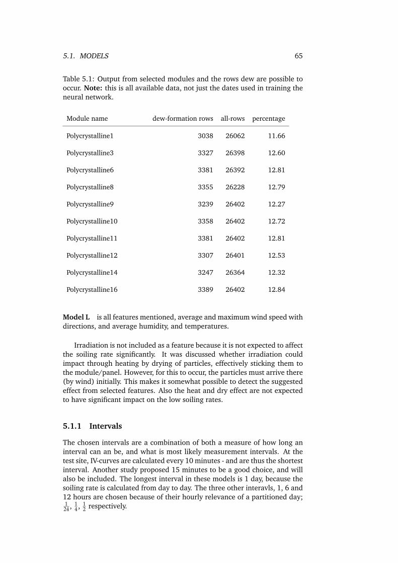
5.1. MODELS 65
Table 5.1: Output from selected modules and the rows dew are possible tooccur. Note: this is all available data, not just the dates used in training theneural network.
Module name dew-formation rows all-rows percentage
Polycrystalline1 3038 26062 11.66
Polycrystalline3 3327 26398 12.60
Polycrystalline6 3381 26392 12.81
Polycrystalline8 3355 26228 12.79
Polycrystalline9 3239 26402 12.27
Polycrystalline10 3358 26402 12.72
Polycrystalline11 3381 26402 12.81
Polycrystalline12 3307 26401 12.53
Polycrystalline14 3247 26364 12.32
Polycrystalline16 3389 26402 12.84
Model L is all features mentioned, average and maximum wind speed withdirections, and average humidity, and temperatures.
Irradiation is not included as a feature because it is not expected to affectthe soiling rate significantly. It was discussed whether irradiation couldimpact through heating by drying of particles, effectively sticking them tothe module/panel. However, for this to occur, the particles must arrive there(by wind) initially. This makes it somewhat possible to detect the suggestedeffect from selected features. Also the heat and dry effect are not expectedto have significant impact on the low soiling rates.
5.1.1 Intervals
The chosen intervals are a combination of both a measure of how long aninterval can an be, and what is most likely measurement intervals. At thetest site, IV-curves are calculated every 10 minutes - and are thus the shortestinterval. Another study proposed 15 minutes to be a good choice, and willalso be included. The longest interval in these models is 1 day, because thesoiling rate is calculated from day to day. The three other interavls, 1, 6 and12 hours are chosen because of their hourly relevance of a partitioned day;1
24 , 14 , 1
2 respectively.

66 CHAPTER 5. ANN IMPLEMENTATION
Table 5.2: An overview of the model inputs, the interval ranges and eachmodel denotation.
Model:Inputs Interval count (length per interval)
1 (1day)
2(12h)
4 (6h) 24(1h)
96(15m)
144(10m)
A: WSavg A0 A1 A2 A3 A4 A5
B: WSavg, WSmax B0 B1 B2 B3 B4 B5
C: WSavgwith wind direc-tions
C0 C1 C2 C3 C4 C5
D: RHavg D0 D1 D2 D3 D4 D5
E: RHavg, Tenv.avg, Tmod.avg E0 E1 E2 E3 E4 E5
F: WSavg, RHavg F0 F1 F2 F3 F4 F5
G: WSavg, WSmax, RHavg G0 G1 G2 G3 G4 G5
H: WSavg, RHavgwith winddirections
H0 H1 H2 H3 H4 H5
I: WSavg, RHavg, Tenv.avg,Tmod.avg
I0 I1 I2 I3 I4 I5
J: WSavg, RHavg, Tenv.avg,Tmod.avgwith wind direc-tions
J0 J1 J2 J3 J4 J5
K: WSavg, WSmax, RHavg,Tenv.avg, Tmod.avg
K0 K1 K2 K3 K4 K5
L: WSavg, WSmax, RHavg,Tenv.avg, Tmod.avgwith winddirections
L0 L1 L2 L3 L4 L5

5.1. MODELS 67
Example of the neural network using one day as interval length gives 10number of hidden nodes from Eq. 3.9 with 71 samples. With one hiddenlayer the ANN can be illustrated by Figure 5.1.
Another example, the maximum number of inputs will be L5. This is10-minute averages and give a total of 144 values for each feature. Thesefeatures are maximum wind speed, average wind speed and humidity, ambienttemperature and module temperature, and the 12 wind directions. The modelrequires 144 ∗ (5 + 12) = 2448 inputs.

68 CHAPTER 5. ANN IMPLEMENTATION
(Model B0)
(Model D0)
Inputs Hidden layer Output
HN1
HNi
HNn..
....
...
....
....
.
Avg_WS
Avg_RH
Soil-rate
wws1
wwsi
wwsn
wrh1
wrhi
wrhn
whn1
whni
whnn
b1
bi
bn
Figure 5.1: Showing the nodes and weight annotations for model F0(combination of B0 and D0), where i = {2, . . . , n − 1} and n = 10. Eachhidden node also has a bias node, in order to shift all values of the activationfunction output.
5.2 Neural net implementation
In ANN, important parameters are the update function and update learningrate, as these two create the foundation for how a neural network willlearn from the training. During experiments on the neural network,update function ADAM (3.8) proved to provide quick and accurate training,requiring less than 100 epochs for the same training result SGD (3.5) aloneneeded more than 10k for. The standard learning rate of 0.02 has also beenchosen as update learning rate, as it had the same performance overall.
Another important feature of an ANN are the layers. The input layer willalways have one node per input multiplied by interval count, ie. ModelsA0 (1 daily WSavg) and B0 (1 daily WSavg and WSmax) will have 1 and 2nodes respectively in the input layer. While A5 and B5 will have 144 and288 input nodes respectively, because there are 144 10m values for eachinput feature. The output layer is one single output node, the soil rate (Sratefrom Eq. 2.17), for all models. The hidden layer have nodes calculated fromEq. 3.9 initially, and will be tested with ±5 nodes. It has been stated morehidden layers are required for non-linear discoveries. Each model are thusavailable to be created with deep learning capabilities. It will be two hiddenlayers for deep learning on models with a single input feature, and threehidden layers for all other models.

5.2. NEURAL NET IMPLEMENTATION 69
5.2.1 Programming tools and libraries
To implement the neural network models, some external Python librariesare used:
• numpy is a well known library for numerical computation (Walt,Colbert, and Varoquaux, 2011).
• Theano is a library for efficiently use of known mathematicalexpressions, integratable with numpy (Al-Rfou et al., 2016).
• Lasagne is a lightweight library for building and training neuralnetworks using Theano (Dieleman et al., 2015). Example of usagefrom lasagne are update functions and layers classes:
– from lasagne.updates import adam– from lasagne.layers import InputLayer, DenseLayer
• NoLearn is a library built upon lasagne, which enables quick imple-mentation of neural networks upon the other libraries (Nouri, 2014).From this library, the ’NeuralNet’ class is imported for quick cre-ation of a neural net using Python-modules from Lasagne: ’fromnolearn.lasagne import NeuralNet’ and its use in this thesis ’Model’class.
def create_net(self,module,epochs=1,update=adam,update_learning_rate=0.02,verbose=False):
"""Creates a neural net with given parameters, andstores it in the local OrderedDict ’nets’ on its’module’ key.:param module: The module name, ie. ’Polycrystalline1’:param epochs: The number of epochs for each training/fiting session:param update: The update function, ie. ’sgd’, ’rmsprop’, ’adam’ oo.:param update_learning_rate: The learning rate, usually 0.01 - 0.02:param verbose: If the NeuralNet is supposed to be verbose or not"""self.nets[module] = NeuralNet(
layers=self.layers,max_epochs=epochs,update=update,objective_loss_function=squared_error,update_learning_rate=update_learning_rate,regression=True,verbose=verbose
)

70 CHAPTER 5. ANN IMPLEMENTATION
5.2.2 Designed classes and functions
Python-module ’learning’ has been created to define the neural net modelclass hierarchy available in the appendix. The most important classes arethe ’Model’ and ’ANN’-classes. The ’Model’ is the superclass of all models,having most of the core functionality like creation of the neural net, fittingtraining data and predicting test data. The ’ANN’-classes define the layerswith single hidden layer (’ANN_Basic’) or multiple layers (’ANN_Advanced’).When initializing either subclassed model, it prepares the input valuesvalues based upon what ’input_keys’ (feature types) are provided usingthe ’extract_inputs_from_keys’ defined.
Each earlier described model has been implemented to automaticallypass the relevant feature keys upward in the class-hierarchy. Thus, theparameters needed for creation of a module are the valid dates, weatherdata (mapping of dates with mapping to all features for each date), the’ProductionData’-module containing production values, and the number ofintervals.

Chapter 6
Results & discussion
This chapter consists of three sections. First a model verification in order toprove the implementation are able to predict known relations. The secondsection is model training with a single hidden layer approach. The lastsection is an attempt at deep learning with 2 and 3 hidden layers.
6.1 Model verification
In order to establish confidence that the suggested models can discover apattern in the data if it exists, a verification using the same principles asanother study (Yadav and Chandel, 2017) were performed. The referencestudy showed the method with best prediction (least MAPE and RMS) onpower output through the day of study occurred when only using irradiationand temperature as inputs for every minute.
Hence an ANN model was built using the same principles as thereference study, using this thesis’ described models to accommodate the twoinputs Iavg and Tenv.avg. There will be one hidden layer with 13 nodes, equalto the model with best results in the reference study. The most notabledifference to the reference study and this dataset is frequency in productionvalues. The Kalkbult data stores production value every 10 minutes, insteadof every minute as was done in the reference study. Due to low irradiancein the morning and evening, values chosen were all 10-minute values from7.30 until and including 17.00, for a total of 58 values for one day.
Three days were chosen for verification; the referance day 11th of May,16th of July, and 16th of September. The first date was used for training, andthe other two for testing. The dates were chosen because it is approximatelythe same length (2 months) between each date. This increases confidencethe model can discover pattern throughout the period of study. In addition,the first two dates are close to clear sky dates, which is shown by a nearperfect circular curve on Figure 6.1a & 6.1b. The last day is a cloudy day,which is indicated by the many dips in the curve on Figure 6.1c. Becausecloudy days are significantly different from clear sky dates, it is a goodverification of the neural network to predict input very different from thetraining dataset.
After training the verification model (hereby known as model) with
71

72 CHAPTER 6. RESULTS & DISCUSSION
07:1
0
08:1
0
09:1
0
10:1
0
11:1
0
12:1
0
13:1
0
14:1
0
15:1
0
16:1
0
17:1
0
t
−0.75
−0.50
−0.25
0.00
0.25
0.50
0.75
1.00
Norm
alize
d va
lues
11th May, training day
TemperatureIrradiationMeasured production
(a) The production in black, irradia-tion in gold and temperature in blueon 11th May.
07:10
08:10
09:10
10:10
11:10
12:10
13:10
14:10
15:10
16:10
17:10
t
−1.00
−0.75
−0.50
−0.25
0.00
0.25
0.50
0.75
Norm
alize
d va
lue
16th July, "clear" day
TemperatureIrradiationMeasured production
(b) The production in black, irradia-tion in gold and temperature in blueon 16th July.
07:1
0
08:1
0
09:1
0
10:1
0
11:1
0
12:1
0
13:1
0
14:1
0
15:1
0
16:1
0
17:1
0
t
−0.5
0.0
0.5
1.0
Norm
alize
d va
lues
16th September, "unclear" day
TemperatureIrradiationMeasured production
(c) The production in black, irradia-tion in gold and temperature in blueon 16th September.
Figure 6.1: These plots show the irradiation and temperature inputs of thethree verification dates, along with production, which is output. Note: Allinput values are normalized in range −1 to 1, and output is normalized inrange 0 to 1 according to Table 4.9.

6.1. MODEL VERIFICATION 73
6 epochs as the reference study suggested, the model did not convergeor score equally well. This may be due to the datasets were different.However this is not likely, as the data in the reference study were similarto the data chosen in this study. A more likely cause was the differentapproaches in training the neural networks. The reference study usedLevenberg–Marquardt (LM) for training, while this thesis used the stochasticgradient descent (SGD) technique ADAM (Eq.3.8). LM is an approxmationto the Newton method, and has the benefit of being faster to find a solutionthan SGD. However, LM needs to be closer to the global minima becauseit does not include momentum which helps ADAM escape a local minima.Beacause of this, additional epochs of training were done on the verificationmodel to a total of 40 epochs. At that point, the verification model had avery good prediction on both the clear and unclear sky days with R2 scoresof 0.963 and 0.845 as shown on Figure 6.2 & 6.3 respectively.

74 CHAPTER 6. RESULTS & DISCUSSION
07:10
08:10
09:10
10:10
11:10
12:10
13:10
14:10
15:10
16:10
17:10
t
0.0
0.2
0.4
0.6
0.8Normalized pr
oduc
tion
16th July, "clear" day
Measured productionPredicted production (R2: 0.963, RMSE: 0.050, MAPE: 12.39)
Figure 6.2: The production in black and predicted data in red on 16th Julywith R2 = 0.963.
07:10
08:10
09:10
10:10
11:10
12:10
13:10
14:10
15:10
16:10
17:10
t
0.2
0.4
0.6
0.8
1.0
1.2
1.4
Normalized production
16th September, "unclear" dayMeasured productionPredicted production (R2: 0.845, RMSE: 0.142, MAPE: 15.55)
Figure 6.3: The production in black and predicted data in red on 16thSeptember with R2 = 0.845.

6.2. SINGLE HIDDEN LAYER (SHL) 75
6.2 Single hidden layer (SHL)
Because the verification model showed 40 epochs of training were necessaryon a dataset with known relation between input and output, each modelfrom Table 5.2 were trained and scored with R2 150 epochs (an entire runthrough the training data with weight updates for each run accordingly).The increase in training epochs were because it is not known how relatedthe features are with soiling, if at all. Also, exploring if this relation exist isthe goal of this thesis.
It is also important to remember the defined soil rate (Srate) is a resultof the change in yield ratio as defined by Eq. 2.17. However, the yieldratio is probably influenced by features besides soiling. This means it isnot guaranteed the target values are only because of soiling. This is alsoindicated on the targets having negative Srate in Figure 6.4 (all values belowthe horizontal 0.5 line). A negative Srate implies a reduction in soiling (animprovement in performance) since the day before. Significant improvementis usually related to cleaning or rain events. Although some studies suggesta minor cleaning event from dew formation can improve performance, andalso powerful wind speeds. That is why the targets are used despite theuncertainty. Additionally, if there is a relationship between a feature andsoiling, they were expected to reduce the magnitude of negative Srate.
6.2.1 Model scores with unsorted inputs
All models were trained and scored with 150 epochs for the 11 differentnode setups in a single hidden layer. The initial hidden nodes werecalculated from Eq. 3.9, and varied with ±5. For each model, the highestvalues of R2 and lowest values for MAPE and RMSE encountered duringtraining of all node setups were stored along with that models scoringhistory. After training and scoring of each node setup, the best R2 valuesencountered were from scoring R2 on the test data (R2
test), while the R2
on whole dataset (R2all) set and training data (R2
train) scores did not showsimilar promise. Additionally the best (lowest) MAPE and RMSE values hadvery poor R2 values.
R2 on the test data
Both the overall and singular best R2 values found were from scoring R2 onthe test data. The best value was ModelD3 with R2
test = 0.225, as shown onTable 6.2.
Model D3 is among the few models with all R2train, R2
test and R2all values
being positive. The other models with all positive R2 scores are the other Dmodels; D4 and D5. This may be due to their positive, albeit low, scoreon R2
train. It was thus not surprising these models held 3/4 top scores.What was surprising is Model D only has RHavg as its sole input feature.Additionally, 8/10 top models had RHavg as one of the input features. Twoother notable inputs were WSavg which is in all models other than D, andWSmax which were in models B, G and K. Comparing the models G2,G3 and

76 CHAPTER 6. RESULTS & DISCUSSION
Table 6.1: A recap on the overview of features and its models with intervaldenotation.
Model:Inputs Length per interval (number of inputs per feature)
1 day(1)
12h(2)
6h (4) 1h(24)
15m(96)
10m(144)
A: WSavg A0 A1 A2 A3 A4 A5
B: WSavg, WSmax B0 B1 B2 B3 B4 B5
C: WSavgwith wind direc-tions
C0 C1 C2 C3 C4 C5
D: RHavg D0 D1 D2 D3 D4 D5
E: RHavg, Tenv.avg, Tmod.avg E0 E1 E2 E3 E4 E5
F: WSavg, RHavg F0 F1 F2 F3 F4 F5
G: WSavg, WSmax, RHavg G0 G1 G2 G3 G4 G5
H: WSavg, RHavgwith winddirections
H0 H1 H2 H3 H4 H5
I: WSavg, RHavg, Tenv.avg,Tmod.avg
I0 I1 I2 I3 I4 I5
J: WSavg, RHavg, Tenv.avg,Tmod.avgwith wind direc-tions
J0 J1 J2 J3 J4 J5
K: WSavg, WSmax, RHavg,Tenv.avg, Tmod.avg
K0 K1 K2 K3 K4 K5
L: WSavg, WSmax, RHavg,Tenv.avg, Tmod.avgwith winddirections
L0 L1 L2 L3 L4 L5

6.2. SINGLE HIDDEN LAYER (SHL) 77
10/05
17/05
24/05
31/05
07/06
14/06
21/06
28/06
05/07
12/07
19/07
26/07
02/08
09/08
16/08
23/08
30/08
06/09
13/09
20/09
27/09
04/10
11/10
18/10
25/10
01/11
08/11
15/11
22/11
29/11
06/12
Target dates
0.400
0.425
0.450
0.475
0.500
0.525
0.550
Norm
alize
d soil-rate
Targets data
Measured normalized soil-rate values
Figure 6.4: The target values with dates and distance from the horizontal0.5 normalized soiling rate implying Srate = 0. Positive values are increasein soiling, and negative values a decrease in soiling (improvement inperformance since last day).
F2 may explain the importance of WSmax and interval lengths. Model G2on rank #8 with all three features are somewhat lower than the similar F2with only WSavg and RHavg on rank #5. The reason for this may be theinterval length and its affect on the feature footprints. Interval-2 is 4 hourintervals, which may not be enough to capture the effect of WSmax in theinterval. Removing the feature could give F2 an advantage over G2 becauseof this. By shortening interval length, model G3 on rank #3 with hourlyvalues (from interval-3) were more likely to catch the effects of WSmax, andis thus the best of the three. Although model B on #6 and #7 consisting ofonly WSavg and WSmax does not support this interval theory, with B1 havinghigher rank than B2. It is worth noting model B is the only model in top10 without RHavg. This could indicate it is better with short intervals whenhaving both RHavg and WSmax as features, but longer intervals are goodenough when only WSavg and WSmax are inputs.
Summarized, these observations indicate the most important featureis humidity (RHavg), along with maximum wind speed (WSmax), andsomewhat average wind speed (WSavg). This is due to humidity beingin almost all models, while average wind speed alone is not among thetop scores. The maximum wind speed seems to be better with decreasinginterval length, but even this value may create noise on the humiditymodels. Without humidity, maximum wind speed had better scores onthe longer intervals (B and F in the table). None of the top ten modelshave wind directions among their inputs at all, indicating these features

78 CHAPTER 6. RESULTS & DISCUSSION
create more noise than they contribute valuable data. Only model K2 onrank #10 had temperatures as input features. Indicating also these featuresprovide more noise than valuable data, although not as bad as the winddirections. The best models usually had hourly intervals (interval-3) on eachinput, with the exception of B and F having best results on 12 (interval-1) and 4 (interval-2) hour intervals respectively. A possible reason forgood scores despite having longer intervals may be the low number of totalinputs. D3 has 1 feature with 24 values to the neural network. By contrastD4 and D5 has 4 and 6 times as many values, 96 and 144 values totalrespectively. These numbers are even higher for the more complex modelswith more than one feature. Because the rate of soiling is likely a non-linearrelationship between humidity, wind, and other features, the relationshipis best captured with lesser values rather than more. Many inputs to theneural network are more likely to contribute noise instead of valuable inputto output relation.
Model D3 prediction
The prediction values on the test data from model D3 at epoch 18, when R2
had best score, is visible on Figure 6.5.The predicted test values (green) against their targets reveal several
of the values are spot on and others really close to their target value.Considering all values are part of the test dataset, and not the trainingdataset, the model has never encountered these inputs and targets. Alsoover half of the points (21/39) are on the correct side of the no-soiling line astheir targets. Although there is no clear pattern if the magnitude increase ordecrease. Looking at the whole dataset in Figure 6.6, the (orange) trainingpredictions does not align good with the (black) measured target values.However, this is not important because it is the unseen values the neuralnetwork is interested in predicting – the test data in this case.
Considering the low RMSE of 0.042 and MAPE of 6.150 together withsome points spot on their targets and the overall good scores of humidity onTable 6.2 indicates there may be some correlation between hourly or shorterRHavg values and the defined Srate.
An observable difference compared to the verification model is the lownumber of epochs, with the best score encountered at 18 epochs. This wasthe best, because it did not encounter a better R2
test in the remaining 132epochs. An explanation for this is the model most overfitted on the trainingdata. This is indeed indicated by looking how R2
test are better than R2train only
early epochs in Figure 6.7, and also by R2train having its best score on epoch
44, much later than 18. The figure stops around 50 epochs, as both scoresgradually worsens and never recover (within the 150 training epochs) asshown in Figure 6.8.
Also, it is important not to let the spike for best R2test value go by
unnoticed. The best score is reached after training from a R2test ≈ 0.01 with
an upward trend to R2test = 0.225. This could indicate among other things
a random hit or too hard learning rate and/or momentum. First, if it were

6.2. SINGLE HIDDEN LAYER (SHL) 79
11/10
18/10
25/10
01/11
08/11
15/11
22/11
29/11
target dates
0.35
0.40
0.45
0.50
0.55
norm
alize
d soil_rate
ModelD3 best R2 test
e18: predicted train, R2: 0.007, RMSE: 0.184, MAPE: 28.287e18: predicted test, R2: 0.225, RMSE: 0.042, MAPE: 6.150measured targets
Figure 6.5: The predictions against their target values for test data usingSHL on unsorted inputs. The black line on 0.5 implies Srate = 0. Severalvalues are spot on, with good R2
test score and low RMSE and MAPE errors.
random – this model and other D models should not hit good on differentnode setups, which also happens on later results. So it is unlikely the inputsand weights happened to hit somewhat good, but it is possible. The morelikely cause is learningrate η = 0.02 and/or momentum α = 0.9 were toopowerful, effectively pushing the network away from from the good weightsunable to recover.
An explanation of the fluctuance in the R2 scores may be the updatefunction or the uncertainties in the target values. The update function usedis ADAM (Eq. 3.8), which includes momentum. This momentum is in placeto push the weight-error function past a local minima. Although on thisdata it looks like it keeps pushing it away from the best minima. This mightbe the result of too strong learning rate or momentum, or the minimas arenot significantly lower than the error function. The uncertainties in targetvalues could lead to inputs with similar footprints having opposite values. Ifsuch values exist, the training of weights may be shifted back and forth foreach epoch (or weight update).
R2 from all data and R2 from training data
The scores encountered on R2all and R2
train are available in the Appendixon Table C.1 & C.2 respectively were not as good as on R2
test, but thereare some elements to look at here as well. However, the primary reasonthese scores are poor is the epoch they mostly occur on is 0. Since thebest scores achieved are encountered after one epoch of training, chance arethe catched relation is more of a coincidence than an actual model of the
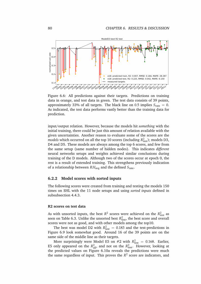
80 CHAPTER 6. RESULTS & DISCUSSION
17/0524/0
531/0
507/0
614/0
621/0
628/0
605/0
712/0
719/0
726/0
702/0
809/0
816/0
823/0
830/0
806/0
913/0
920/0
927/0
904/1
011/1
018/1
025/1
001/1
108/1
115/1
122/1
129/1
1
target dates
0.1
0.2
0.3
0.4
0.5norm
alize
d soil_rate
ModelD3 best R2 test
e18: predicted train, R2: 0.007, RMSE: 0.184, MAPE: 28.287e18: predicted test, R2: 0.225, RMSE: 0.042, MAPE: 6.150measured targets
Figure 6.6: All predictions against their targets. Predictions on trainingdata in orange, and test data in green. The test data consists of 39 points,approximately 33% of all targets. The black line on 0.5 implies Srate = 0.As indicated, the test data performs vastly better than the training data forprediction.
input/output relation. However, because the models hit something with theinitial training, there could be just this amount of relation available with thegiven uncertainties. Another reason to evaluate some of the scores are themodels which occurred on all the top 10 scores (including R2
test); models D3,D4 and D5. These models are always among the top 6 scores, and few fromthe same setup (same number of hidden nodes). This indicates differentneural networks setups and weights achieved similar conclusions duringtraining of the D models. Although two of the scores occur at epoch 0, therest is a result of extended training. This strengthens previously indicationof a relationship between RHavg and the defined Srate.
6.2.2 Model scores with sorted inputs
The following scores were created from training and testing the models 150times on SHL with the 11 node setups and using sorted inputs defined insubsubsection 4.4.3.
R2 scores on test data
As with unsorted inputs, the best R2 scores were achieved on the R2test as
seen on Table 6.3. Unlike the unsorted best R2test, the best score and overall
scores were not as good, and with other models among the top10.The best was model D2 with R2
test = 0.183 and the test-predictions inFigure 6.9 look somewhat good. Around 16 of the 39 points are on thesame side of the middle line as their targets.
More surprisingly were Model E5 on #2 with R2test = 0.168. Earlier,
E5 only appeared on the R2all, and not on the R2
test. However, looking atthe predicted values on Figure 6.10a reveals the predictions were muchthe same regardless of input. This proves the R2 score are indicators, and

6.2. SINGLE HIDDEN LAYER (SHL) 81
Table 6.2: The top 10 best R2 values encountered on the test data with SHLon unsorted inputs.
# Model Hiddennodes
epoch R2train R2
test R2 RMSE MAPE
1 ModelD3 14(+2) 18 0.016 0.225 0.013 0.042 6.150
2 ModelD5 7(-5) 20 0.002 0.198 0.026 0.066 10.578
3 ModelG3 18(+5) 4 -0.150 0.195 -0.035 0.051 8.994
4 ModelD4 17(+5) 12 0.010 0.147 0.008 0.072 11.939
5 ModelF2 10(-3) 6 -0.343 0.145 -0.182 0.033 5.108
6 ModelB1 8(-5) 5 -0.147 0.137 -0.054 0.048 7.387
7 ModelB3 8(-5) 16 -0.136 0.126 -0.043 0.055 9.374
8 ModelG2 14(+1) 4 -0.053 0.118 0.009 0.075 12.779
9 ModelG1 12(-1) 0 -0.064 0.097 -0.005 0.080 12.404
10 ModelK2 17(+3) 29 -0.027 0.093 0.020 0.065 10.878
Table 6.3: The top 10 best R2 values encountered using SHL on the test datawith sorted inputs have a little lower values than the unsorted scores on testdata.
# Model Hiddennodes
epoch R2train R2
test R2 RMSE MAPE
1 ModelD2 7(-5) 14 0.004 0.183 -0.004 0.042 6.545
2 ModelE5 10(-3) 16 -0.010 0.168 -0.023 0.038 5.610
3 ModelF2 9(-4) 10 0.001 0.160 -0.010 0.042 7.064
4 ModelG3 13 8 -0.024 0.132 0.032 0.070 11.207
5 ModelE4 11(-2) 18 -0.010 0.130 -0.018 0.066 11.753
6 ModelD4 15(+3) 11 0.004 0.129 0.000 0.069 11.464
7 ModelG4 10(-3) 18 -0.007 0.122 -0.020 0.044 7.465
8 ModelI5 19(+5) 8 -0.008 0.118 -0.021 0.045 7.534
9 ModelF5 13 16 0.003 0.115 -0.001 0.065 10.987
10 ModelI2 13(-1) 12 -0.070 0.094 -0.031 0.033 5.436

82 CHAPTER 6. RESULTS & DISCUSSION
0 10 20 30 40epochs
−0.1
0.0
0.1
0.2
0.3R2
score
Max R2_train: 0.039 (e44)
Max R2_test: 0.225 (e18)
Model D3 R2 scoresR2_trainR2_test
Figure 6.7: The scores of Model D3, with the maximum points annotated.
prediction plots are needed for confirmation. Although the two lowest targetvalues received yet again indication of prediction. From other predictionplots, both values, with the last especially, are often well predicted. Becausethe R2 only can be used as indication, the rest of top 10 R2
test prediction plotsare included in the Appendix in subsection C.1.
From all the prediction plots for the sorted input scores, both E4 andE5, together with I5, show poor predictions contrary to their R2
test scores.These models similarities are their temperature features (Tenv.avg, Tmod.avg)and the short intervals of 10 and 15 minutes. Only model I2 on #10 includestemperatures as feature, but this model has 6 hour intervals. It is thussuspected the sorted temperatures contribute more noise than valuable datafor shorter intervals. A last interesting observation from the R2
test values areRHavg is a feature in every model.
R2 scores on train and all data
The R2all scores on Table C.4 looks more poor than the R2
all scores from theunsorted input, both top score and in general. Still, some interesting trendscontinues with Model D3, D4 and D5 again among the top 10, togetherwith F3 and G3. The most notable difference is model I2 and I3 are presenton the sorted input scores. Model I were not among top 10 on any of theunsorted runs. It may seem that sorting the temperature features on thelonger intervals provide new models some valuable data, but in general thesorting of input features lowers scoring on the previously well performingmodels.

6.2. SINGLE HIDDEN LAYER (SHL) 83
0 20 40 60 80 100epochs
−1.0
−0.8
−0.6
−0.4
−0.2
0.0
0.2
0.4
R2 sc
ore
Max R2_train: 0.039 (e44)
Max R2_test: 0.225 (e18)
Model D3 R2 scoresR2_trainR2_test
Figure 6.8: The unzoomed scores of Model D3, with the maximum pointsannotated.
Finally, the R2train scores on Table C.5 in the appendix continues R2
allobservation with most models the same as in the unsorted score. Onesurprise is the addition of I5 on the top spot. However, the score of R2
train isagain not representative for prediction when looking at the poor predictionsin Figure 6.11.

84 CHAPTER 6. RESULTS & DISCUSSION
11/10
18/10
25/10
01/11
08/11
15/11
22/11
29/11
target dates
0.35
0.40
0.45
0.50
0.55
norm
alize
d soil_rate
ModelD2
e14: predicted test, R2: 0.182, RMSE: 0.041, MAPE: 6.474measured targets
Figure 6.9: The test predictions values against their target values for ModelD2 with SHL and sorted input features. There are a few predictions spot ontheir targets, but most is opposite of their measured value.

6.2. SINGLE HIDDEN LAYER (SHL) 85
11/10
18/10
25/10
01/11
08/11
15/11
22/11
29/11
target dates
0.35
0.40
0.45
0.50
0.55
norm
alize
d soil_rate
ModelE5e16: predicted test, R2: 0.168, RMSE: 0.037, MAPE: 5.524measured targets
(a) The test predictions values against their target values for Model D2 with SHLand sorted input features.
10/0517/0
524/0
531/0
507/0
614/0
621/0
628/0
605/0
712/0
719/0
726/0
702/0
809/0
816/0
823/0
830/0
806/0
913/0
920/0
927/0
904/1
011/1
018/1
025/1
001/1
108/1
115/1
122/1
129/1
106/1
2
target dates
0.25
0.30
0.35
0.40
0.45
0.50
0.55
norm
alize
d soil_rate
ModelE5
e16: predicted train, R2: -0.010, RMSE: 0.195, MAPE: 34.691e16: predicted test, R2: 0.168, RMSE: 0.037, MAPE: 5.524measured targets
(b) All predictions against their targets for E5 with sorted input features and SHL.Again, predictions on training data are poor compared to the predictions on testdata.
Figure 6.10: The best predictions for Model E5 for whole data and test datausing sorted input features and SHL.

86 CHAPTER 6. RESULTS & DISCUSSION
17/0524/0
531/0
507/0
614/0
621/0
628/0
605/0
712/0
719/0
726/0
702/0
809/0
816/0
823/0
830/0
806/0
913/0
920/0
927/0
904/1
011/1
018/1
025/1
001/1
108/1
115/1
122/1
129/1
1
target dates
0.25
0.30
0.35
0.40
0.45
0.50
0.55
0.60
norm
alize
d soil_rate
ModelI5e25: predicted train, R2: 0.062, RMSE: 0.092, MAPE: 14.093e25: predicted test, R2: -0.169, RMSE: 0.083, MAPE: 15.078measured targets
Figure 6.11: The predictions values against all targets on ModelI5 fromthe best R2
train scores. However, it does not show much variance in outputtargets.

6.3. DEEP LEARNING MODELS 87
6.3 Deep learning models
The deep learning (DL) models were trained and scored similar to the singlelayer models, 150 times for 11 different node setups. The only difference isthe hidden layers consists of either 2 or 3 layers, depending on the numberof inputs to the models. For each change in node count, all layers arechanged. This means all the hidden layers have the same number of nodesat all times.
6.3.1 Model scores with unsorted input features
The R2 scores encountered during training and scoring the deep ANNs aremuch alike the single layered setups on R2
test values. Additionally, the deeplearning setups encountered better R2
train scores.The most exciting result from deep learning was model D again
achieving the best score on both R2train and R2
test. Again indicating theinfluence humidity has on the Srate. One difference from the single hiddenlayer scores were the setups hitting top spots were models with more(and thus shorter) intervals; D4 and D5 with 10 and 15 minute intervalsrespectively. Except on R2
all, which is held by E5 (1st), E3 (2nd) and E4(3rd). Model E consists of humidity (RHavg) and the average temperatures(Tenv.avg and Tmod.avg). This confirms deep learning is better to identifythe non-linear relationships between features. As such, better results frommodels with more input features are expected by using deep learning. Thisincludes shorter intervals, as the increase in inputs from the intervals canresemble non-linear interfeature relationships. The most surprising score isB1 on #5 with R2
test = 0.106. B1 has 4 inputs, WSavg and WSmax averagedand maxed over 12 hours. Model B had decent scores on both single hiddenlayer and deep learning, and both times with few (long) interval counts.This indicates the WSmax is the most important feature – as this value isnot averaged, but the maximum value within the period. If WSavg werethe significant feature, more shorter intervals would be expected to performbetter with deep learning. However, the longer and few intervals were beston both approaches – indicating WSmax are the important feature of the two.
Predictions
Looking at the predicted values for D5 (best on R2test) and E5 (best on R2
all)in Figures 6.12 & 6.13, it seems like E5 is better suited to become a moregeneral model than D5, despite D5’s better R2 score.
Other interesting predictions from the deep learning score tables are thebetter results from Model K5. K5 is the combination of nearly all features(RHavg, WSavg, WSmax, Tenv.avg, Tmod.avg), and has rank #4 on R2
test and #9on R2
all. The predictions on (unseen) test data for K5 in Figure 6.14 fromR2
test shows similar promise as the other models visually prediction plots. Itis also worth noting K5 has both lowest RMSE and MAPE of all the top 10

88 CHAPTER 6. RESULTS & DISCUSSION
Table 6.4: The top 10 best R2 values encountered on the train data of deeplearning models with unsorted input features had better scores than the SHLsetup.
# Model Hiddennodes
epoch R2train R2
test R2 RMSE MAPE
1 ModelD4 16(+4) 54 0.179 -1.516 -0.357 0.047 6.113
2 ModelD5 16(+4) 149 0.115 -0.584 0.023 0.050 8.057
3 ModelE5 16(+3) 45 0.077 -0.014 0.042 0.090 13.467
4 ModelE4 8(-5) 46 0.065 -0.062 0.030 0.093 16.097
5 ModelE3 16(+3) 2 0.042 0.009 0.042 0.131 22.301
6 ModelG4 12(-1) 13 0.042 -0.170 -0.031 0.074 12.582
7 ModelG1 9(-4) 5 0.033 -0.031 -0.016 0.166 32.753
8 ModelI5 14 10 0.029 -0.007 0.009 0.524 94.163
9 ModelD3 10(-2) 13 0.029 -0.004 0.004 0.120 22.740
10 ModelF4 12(-1) 5 0.024 -0.015 -0.012 0.246 46.221
Table 6.5: The top 10 best R2 values encountered on the test data of deeplearning models with unsorted feature inputs had somewhat similar scoresas the SHL.
# Model Hiddennodes
epoch R2train R2
test R2 RMSE MAPE
1 ModelD5 15(+3) 7 -0.025 0.243 -0.013 0.069 11.494
2 ModelD4 11(-1) 7 -0.044 0.217 -0.006 0.057 10.164
3 ModelF4 11(-2) 4 -0.058 0.112 -0.018 0.090 15.313
4 ModelK5 13(-1) 9 -0.002 0.107 0.009 0.049 7.877
5 ModelB1 10(-3) 6 -0.190 0.106 -0.054 0.064 10.176
6 ModelG4 13 24 -0.020 0.103 0.000 0.068 10.520
7 ModelE4 17(+4) 3 0.004 0.080 -0.000 0.066 10.609
8 ModelG5 12(-1) 7 0.007 0.080 0.026 0.136 20.752
9 ModelD2 13(+1) 3 0.001 0.074 -0.001 0.072 11.828
10 ModelA4 7(-5) 1 -0.035 0.068 0.000 0.148 25.637

6.3. DEEP LEARNING MODELS 89
11/10
18/10
25/10
01/11
08/11
15/11
22/11
29/11
target dates
0.200.250.300.350.400.450.500.55
norm
alize
d soil_rate
Model D5
e7: predicted train, R2: -0.036, RMSE: 0.218, MAPE: 33.600e7: predicted test, R2: 0.243, RMSE: 0.069, MAPE: 11.494measured targets
Figure 6.12: The predicted values against their targets for Model D5 usingdeep layer and unsorted input features. This was best R2
test score of theunsorted deep learning models.
models from R2test scores on Table 6.5. This indicates the values are closest
to the mean of the targets.Lastly, the predictions from the model B1 on Figure 6.15 have nearly the
same values and scores as K5, with a slight tendency to align to the middlescore of 0.5.
6.3.2 Model scores with sorted input features
The sorted models were run with the same 11 different node setups with150 epochs and 2 or 3 layers, with 1 or more feature types respectively.Again the best R2 score encountered where overall and best from R2
testasseen on Table 6.6.
However, unlike the poor results from sorted input features with SHL,these scores included the best score encountered of all tables with Model D4having R2
test = 0.267. Which is around 10% better than D5’s R2test = 0.243
from the unsorted input features with deep learning. In addition, the otherscores from top 10 where somewhat better than the R2
test scores for theunsorted input features. A similar observation on both sorted and unsortedruns are the low presence of the most complex models. K5 were the onlyone in both top 10 R2
test scores, and has the shortest intervals and all featuresexcept wind directions with 576 input nodes. However, the best scores usingsorted input features had generally shorter (and thus more) intervals.
From these observations, it may indicate the sorting of input featuresare more important in non-linear relationships. As deep learning is better onnon-linear relationships, and the sorted input features had both general bestand highest score. This was also the reason for sorting the input features– to capture the interaction between features regardless of time of day theyhappened.

90 CHAPTER 6. RESULTS & DISCUSSION
11/10
18/10
25/10
01/11
08/11
15/11
22/11
29/11
target dates
0.30
0.35
0.40
0.45
0.50
0.55
0.60no
rmalize
d soil_rate
Model E5
e32: predicted train, R2: -0.008, RMSE: 0.081, MAPE: 13.046e32: predicted test, R2: 0.019, RMSE: 0.080, MAPE: 11.837measured targets
Figure 6.13: The predicted values against their targets for Model E5 usingdeep layer and unsorted input features. It had the best R2
all score of the deeplearning models.
Prediction plots
Looking at the prediction plots for the top three models from Table 6.6, D4,F4 and D3 in Figures 6.16, 6.17 & 6.18 respectively, the R2
test score indicationcorresponds with the prediction values. Both D3 and D4 has RHavg as itsonly input feature, whereas F4 also includes WSavg together with RHavg. Itis difficult to be conclusive, but with 26 targets on the same side of Srate = 0as their targets, F4 may be more aligned its targets than D3 and D4. Allthree have some points spot on, although, not the same targets. This isexpected between model types, but D3 and D4 should be more aligned.An explanation might lie in the neuron weights and the minima they startout from and end up with are different because of the interval lengths andinputs.
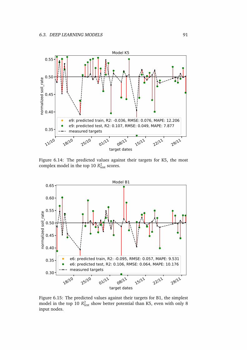
6.3. DEEP LEARNING MODELS 91
11/10
18/10
25/10
01/11
08/11
15/11
22/11
29/11
target dates
0.35
0.40
0.45
0.50
0.55
norm
alize
d soil_rate
Model K5
e9: predicted train, R2: -0.036, RMSE: 0.076, MAPE: 12.206e9: predicted test, R2: 0.107, RMSE: 0.049, MAPE: 7.877measured targets
Figure 6.14: The predicted values against their targets for K5, the mostcomplex model in the top 10 R2
test scores.
18/10
25/10
01/11
08/11
15/11
22/11
29/11
target dates
0.30
0.35
0.40
0.45
0.50
0.55
0.60
0.65
norm
alize
d soil_rate
Model B1
e6: predicted train, R2: -0.095, RMSE: 0.057, MAPE: 9.531e6: predicted test, R2: 0.106, RMSE: 0.064, MAPE: 10.176measured targets
Figure 6.15: The predicted values against their targets for B1, the simplestmodel in the top 10 R2
test show better potential than K5, even with only 8input nodes.

92 CHAPTER 6. RESULTS & DISCUSSION
Table 6.6: The top 10 best R2 values encountered on the test data of deeplearning models with sorted input features encountered generally higherscores, including the highest before the last run available in appendix..
# Model Hiddennodes
epoch R2train R2
test R2 RMSE MAPE
1 ModelD4 17(+5) 3 -0.015 0.267 -0.004 0.065 10.398
2 ModelF4 11(-2) 21 -0.123 0.214 0.012 0.068 11.045
3 ModelD3 14(+2) 5 0.009 0.202 0.002 0.040 6.377
4 ModelF5 8(-5) 55 -0.046 0.141 0.016 0.061 9.914
5 ModelB3 8(-5) 149 -2.121 0.139 -0.180 0.037 5.022
6 ModelK5 13(-1) 2 -0.013 0.127 -0.023 0.042 6.704
7 ModelD5 10(-2) 23 -0.018 0.126 -0.028 0.054 7.765
8 ModelB4 13 13 -0.080 0.125 0.009 0.070 9.849
9 ModelE5 9(-4) 3 -0.069 0.125 -0.044 0.075 11.459
10 ModelG4 16(+3) 33 -0.019 0.094 0.014 0.064 10.556
11/10
18/10
25/10
01/11
08/11
15/11
22/11
29/11
target dates
0.30
0.35
0.40
0.45
0.50
0.55
0.60
norm
alize
d soil_rate
ModelD4
e3: predicted test, R2: 0.268, RMSE: 0.065, MAPE: 10.202measured targets
Figure 6.16: Prediction values against their test targets for the bestencountered model, D4, with deep learning and sorted input features.

6.3. DEEP LEARNING MODELS 93
11/10
18/10
25/10
01/11
08/11
15/11
22/11
29/11
target dates
0.25
0.30
0.35
0.40
0.45
0.50
0.55
0.60
norm
alize
d soil_rate
ModelF4e21: predicted test, R2: 0.206, RMSE: 0.070, MAPE: 11.329measured targets
Figure 6.17: The prediction values against their targets for Model F4, thenext best encountered model with deep learning and sorted input features.The values are more spread than the best model.
11/10
18/10
25/10
01/11
08/11
15/11
22/11
29/11
target dates
0.40
0.45
0.50
0.55
0.60
norm
alize
d soil_rate
ModelD3e5: predicted test, R2: 0.201, RMSE: 0.040, MAPE: 6.340measured targets
Figure 6.18: The predicted values against their targets for Model D3, thethird best encountered score with deep learning and sorted input features.Although some values are spot on, most seem to go too high, suggestingpoor predictability.

94 CHAPTER 6. RESULTS & DISCUSSION

Chapter 7
Conclusion &recommendations
This chapter try to give som conclusive remarks regarding the results, andsuggests recommendations for future work.
7.1 Feature relationship
The final goal of this thesis was to investigate suggested environmentalvariables relationship with daily soiling, by evaluating with machinelearning. Although no conclusive relationship between the features andthe defined soiling rate could be established, there are strong indicationshumidity is an important feature for the daily change yield ratio.
Applying more features together with humidity did not directly improvethis indication. However, it did establish some more confidence to theindication of humidity having an influence on the defined Srate. Nearlyall models for every top 10 scores had humidity as a part of the featureinputs. Usually the models with the best scores on the table also had eitherhumidity alone, or with few other features like average or maximum windspeed. Among the deep learning scores, humidity still played an importantrole with the larger models, even when only humidity was input. However,with deep learning more complex and non-linear relationships indicatedmaximum wind speed also has somewhat influence. Even more so withmore (and shorter) intervals. This proved especially true using sorted inputfeatures, where average humidity and wind speed seemed like the bestcandidate of the presented predictions.
In addition, these results comply with what was expected from otherstudies in soiling. Together with the fact that several predicted valueswere spot on their target values. If more confidence were established thatthe defined Srate are related to soiling, those targets would be strongerindications. As of now, the defined Srate are likely affected by other factors,making it uncertain if the predicted targets are a result of soiling – orsomething else.
A conclusion that can be done with the achieved scores are winddirections seem to cause more noise as than valuable data. This is because
95

96 CHAPTER 7. CONCLUSION & RECOMMENDATIONS
none of the top ten models in any score table had wind directions as itsinput features.
Some possible reasons the results are as they are:
• Preprocessing of data to feed a neural network is essential. Nearlyhalf of the available input data were removed due to inconsistenciesor clearly not target values because of soiling. In the early stages ofpredictions, R2 scores with negative scores in the scale of 1000 wereachieved. By removing the erronous values, the end results showedmuch more consistent outputs.
• Normalization of the output values may have improved performance.Both larger and lower values were used earlier in the process withworse results. Although this could be due to other factors likeupdate function, layer setup or valid dates or other, because noneof the mentioned could be confirmed constant during the change tonormalized targets.
• Neural network parameters are important. Another early discoverywere the use of correct update function. Using regular SGD as updaterequired several thousand epochs of training to achieve decent R2
values. With research and discovery of RMSProp and ADAM, therequired epochs and time were severely reduced. The change inupdate function also gave better results.
• The results seems to comply with the neural networks ability to detectnon-linear relationships, only when hidden layers are more than one.This is what has been suggested by studies into ANN, and thus why itwas included. With a single hidden layer, the lower input and intervalmodels scored better, as was expected. With 2 and 3 hidden layers,more complex models achieved better scores, as expected. Deeplearning is thus recommended when trying to investigate several inputfeatures or interval relationships.
It is planned to make all code public, if this is not possible or has nothappened at the time of reading, but are desired -– contact author to ask foraccess to the private Git repository.
7.2 Recommendations for future work
Although the results of this thesis cannot conclude a relationship, theindications do provide some direction on where to go next.
7.2.1 Secure more reliable data
The data used in this project were quite unreliable. There were severaldates were data was missing, and even wrong in the way it does not makesense. As an example, ambient temperatures above 170°C is not a reliablevalue to process. The need to assure such values are not part of datasets are

7.2. RECOMMENDATIONS FOR FUTURE WORK 97
important, but time consuming and in worst case renders input or outputvalues erronous and useless. It may also be somewhat more accurate to usea two-diode-model instead of single-diode model for calculating maximumpower point of the modules. However, given the uncertainties mentionedthis is not expected to impact much.
7.2.2 Include data/measurement of airborne particles
A recent study indicated the particle composition of the air could predictsoiling levels by around 80% (Micheli and Muller, 2017). Including thesefeatures as inputs would be expected to increase prediction accuracy. Withbetter accuracy it could also indicate how well this model performed bycomparing with and without the particle composition.
7.2.3 Daily cleaning of a reference module
This is likely the single most important recommendation for next step in theinvestigation of soiling. The uncertainties in this thesis output values couldbe the reason higher predictions were not achieved. With higher degree ofcertainty the target values are only because of soiling, a relationship may bediscovered. The other studies within the same project showed module yieldratio is highly dependent on the magnitude of irradiance, using the definedSrate based upon this irradiance are suspected to be the main source of errorin target values. Having the possibility of comparing a dirty module againsta clean module on a daily basis would remove this dependency.
7.2.4 Expanding the neural network
As each model only had 11 different setups based upon their input nodes,considering using other update functions, learning rates, momentum valuesand other machine learning parameters could improve performance of theneural network. Learning rates of 0.015 and 0.01 were done earlier in thethesis. However, they did not improve the performance at that point. Withbetter datasets as mentioned previously, this might change.
7.2.5 Other machine learning techniques
Artificial neural network are good predictors, the one used in this thesis arenot the only way to use it. Two other neural network approaches consideredwere:
• Recurrent neural network (RNN) discussed in Chapter 3 are indicatedto be the best regression-predicting machine learning algorithm thereis. However, it is harder to implement than regular ANN and with thisthesis varying date of input, having a recurring loop from previousvalues would not be as beneficial. If data were more reliable andbetter with higher resolution – a daily footprint could be capturedby the RNN instead of feeded as daily value. RNN would then berecommended.

98 CHAPTER 7. CONCLUSION & RECOMMENDATIONS
• Convolutional neural network (CNN) were considered. Although CNNsare best at classification tasks, the reason it was considered was bypicturing the daily footprint as an image, ie. For an hourly model, allinput features would be on the Y-axis, and the hours would be the X-axis, creating a 2-dimensional grid of the footprint. This would enablea more concise footprint of the daily values than the densely connectedANN used in this thesis.
Other machine learning algorithms unrelated to neural networks areavailable to be used with regression. Some suggestions are Support VectorMachines (SVM) and k-Nearest-Neighbours (kNN).
7.2.6 Increase the dataset
A longer period of study for more data points usually increases machinelearning performance on both unique/special conditions and core values.Because the core values would likely be trained more often, and theunique/special conditions are thus observerd at least once, influencing themodel training.

Appendices
99


Appendix A
Issues with weather data
101

102 APPENDIX A. ISSUES WITH WEATHER DATA
Table A.1: First the interpolated dates and their row counts, and thenthe invalid dates and their row counts. The date with 1441 values had aduplicate that was removed.
Interpolated dates
Date 19/05 06/06 19/06 12/08 14/09 11/10 24/11
rows 1438 1397 1441 1436 1437 1439 1435
Invalid dates
Date 08/06 21/06 22/06 24/06 25/06 26/06 27/06 29/06 30/06
rows 866 545 0 0 371 338 516 0 99
Date 01/07 02/07 03/07 04/07 06/07 07/07 09/07 11/07 12/07
rows 377 161 408 293 0 520 679 0 272
Date 13/07 13/08 02/09 13/09
rows 706 1167 0 0

Appendix B
UML diagrams
B.1 Data collection
103
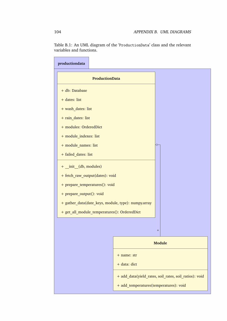
104 APPENDIX B. UML DIAGRAMS
Table B.1: An UML diagram of the ’ProductionData’ class and the relevantvariables and functions.
productiondata
*
ProductionData
+ db: Database
+ dates: list
+ wash_dates: list
+ rain_dates: list
+ modules: OrderedDict
+ module_indexes: list
+ module_names: list
+ failed_dates: list
+ __init__(db, modules)
+ fetch_raw_output(dates): void
+ prepare_temperatures(): void
+ prepare_output(): void
+ gather_data(date_keys, module, type): numpy.array
+ get_all_module_temperatures(): OrderedDict
Module
+ name: str
+ data: dict
+ add_data(yield_rates, soil_rates, soil_ratios): void
+ add_temperatures(temperatures): void

B.2. MODELS 105
B.2 Models
Table B.2: An UML diagram of the ’Model’ class and its variables andfunctions.
learning
Model
+ input_keys: list
+ X: numpy.array
+ layers: list
+ nets: OrderedDict
+ module_inputs: OrderedDict
+ label: str
+ __init__(keys, input_values, productiondata, input_keys, interval, label)
+ create_net(module, ...): void
+ create_nets(modules, ...): void
+ fit(module, train_percent=0.66): void
+ fit_all(train_percent=0.66): void
+ predict(module, X=None): numpy.array
+ training_inputs(start_index, end_index, module): numpy.array
+ test_inputs(pivot, module): numpy.array
+ prepare_targets(module, y_type=’soil_rates’): None

106 APPENDIX B. UML DIAGRAMS
Table B.3: An UML diagram of the subclasses of ’Model’.
learning
Model
Model_Verification
+ targets: OrderedDict
+ dates: list
+ layers: list
ANN
+ productiondata: ProductionData
+ keys: list
+ module_temperatures: OrderedDictionary
+ __init__(keys, input_values, productiondata, input_keys, interval, label)
+ prepare_module_temperatures(interval): void
+ prepare_inputs(module=None): numpy.array
+ increment_nodes(incr): void
+ decrement_nodes(decr): void
+ get_num_nodes(layer): int

B.2. MODELS 107
Table B.4: An UML diagram of the two subclasses for ’ANN’. They specifydifferent layer setups with regards to their initialization.
learning
ANN
Basic
+ layers: list
+ __init__(date_keys, input_values, productiondata, input_keys, interval, label)
Advanced
layers: list
+ __init__(date_keys, input_values, productiondata, input_keys, interval, label)

108 APPENDIX B. UML DIAGRAMS
Table B.5: An UML diagram of all subclasses for both ’Basic’ and ’Advanced’.These are the model classes that are initialized, and have predefined’input_keys’ as shown in notes for most classes.
learning
Basic
Advanced
Model_A
+ __init__(date_keys, input_values, productiondata, interval, advanced)
input_keys = [’Avg_WS’]input_keys = [’Avg_WS’]
Model_B
input_keys = [’Avg_WS’, ’Max_WS’]input_keys = [’Avg_WS’, ’Max_WS’]
Model_C
input_keys = [’Avg_WS’, ’Max_WS’, wind_dirs]input_keys = [’Avg_WS’, ’Max_WS’, wind_dirs]
Model_D
input_keys = [’Avg_RH’]input_keys = [’Avg_RH’]
Model_E
input_keys = [’Avg_RH’, ’Avg_Tamb’, ’Avg_Tmod’]input_keys = [’Avg_RH’, ’Avg_Tamb’, ’Avg_Tmod’]
Model_F
input_keys = [’Avg_RH’, ’Avg_WS’]input_keys = [’Avg_RH’, ’Avg_WS’]
Model_G
input_keys = [’Avg_RH’, ’Avg_WS’, ’Max_WS’]input_keys = [’Avg_RH’, ’Avg_WS’, ’Max_WS’]
Model_H
input_keys = [’Avg_RH’, ’Avg_WS’, wind_dirs]input_keys = [’Avg_RH’, ’Avg_WS’, wind_dirs]
Model_I
(...)(...)
Model_J
(...)(...)
Model_K
(...)(...)
Model_L
(...)(...)

Appendix C
Additonal result tables andplots
C.1 Unsorted inputs SHL second run and plots
First are the R2train and R2 scores for SHL unsorted input features on
Table C.1Because results were lost, a second run with SHL on unsorted input
features were run. The scores are presented on Table C.3. The scorescomply almost directly with the previous achieved scores. This gives furtherconfidence on the models that gives the best scores, as once again Model Dachieves new highscore, with R2
test = 0.286.
109

110 APPENDIX C. ADDITONAL RESULT TABLES AND PLOTS
Table C.1: The top 10 best R2 values encountered with SHL on whole datafor unsorted input features.
# Model Hiddennodes
epoch R2train R2
test R2 RMSE MAPE
1 ModelE3 14(+1) 0 0.059 0.024 0.059 0.121 21.188
2 ModelE5 11(-2) 0 0.077 -0.035 0.052 0.085 13.380
3 ModelD3 7(-5) 5 0.039 0.040 0.039 0.122 20.711
4 ModelF4 9(-4) 0 0.033 0.067 0.035 0.104 18.048
5 ModelD5 7(-5) 21 0.005 0.165 0.035 0.067 10.341
6 ModelD4 7(-5) 0 0.042 0.034 0.033 0.153 27.680
7 ModelI3 14 0 0.010 0.001 0.027 0.048 7.859
8 ModelG3 17(+4) 3 -0.021 0.055 0.026 0.181 27.986
9 ModelF2 11(-2) 4 0.012 0.084 0.025 0.054 9.014
10 ModelF3 11(-2) 0 0.044 -0.028 0.024 0.050 7.640
Table C.2: The top 10 best R2 values encountered with SHL on the trainingdata for unsorted input features.
# Model Hiddennodes
epoch R2train R2
test R2 RMSE MAPE
1 ModelE3 13 2 0.082 -0.017 0.036 0.162 27.662
2 ModelE5 11(-2) 0 0.077 -0.035 0.052 0.085 13.380
3 ModelD4 7(-5) 11 0.065 0.010 0.030 0.122 21.741
4 ModelD5 15(+3) 0 0.050 0.021 0.034 0.161 26.538
5 ModelD3 10(-2) 68 0.049 -0.147 -0.014 0.056 9.135
6 ModelE2 11(-2) 6 0.047 -0.191 0.016 0.052 8.391
7 ModelF3 11(-2) 0 0.044 -0.028 0.024 0.050 7.640
8 ModelF4 9(-4) 0 0.033 0.067 0.035 0.104 18.048
9 ModelF5 13 20 0.022 -0.087 0.001 0.095 15.951
10 ModelD2 17(+5) 10 0.021 -0.026 -0.022 0.113 22.094

C.1. UNSORTED INPUTS SHL SECOND RUN AND PLOTS 111
11/10
18/10
25/10
01/11
08/11
15/11
22/11
29/11
target dates
0.30
0.35
0.40
0.45
0.50
0.55
norm
alize
d soil_rate
ModelD3
e2: predicted test, R2: 0.283, RMSE: 0.054, MAPE: 7.932measured targets
Figure C.1: The test predictions values against their target values for ModelD3, #1 from last runs R2
test with SHL and unsorted inputs.
Table C.3: The top 10 best R2 values encountered on the test dataset after asecond run with unsorted inputs on SHL.
# Model Hiddennodes
epoch R2train R2
test R2 RMSE MAPE
1 ModelD3 7(-5) 2 -0.008 0.286 0.006 0.055 7.932
2 ModelD2 11(-1) 11 0.002 0.245 -0.004 0.041 6.802
3 ModelD5 7(-5) 10 0.006 0.216 0.003 0.064 9.856
4 ModelG5 18(+5) 9 0.002 0.199 -0.004 0.055 9.985
5 ModelG2 16(+3) 27 -0.053 0.170 0.016 0.069 11.609
6 ModelD4 15(+3) 17 0.006 0.144 0.004 0.102 15.723
7 ModelF3 8(-5) 3 -0.077 0.138 -0.025 0.055 9.418
8 ModelK1 12(-2) 14 -0.062 0.123 0.031 0.065 10.996
9 ModelE2 14(+1) 2 0.007 0.095 -0.002 0.061 10.353
10 ModelG3 11(-2) 30 -0.182 0.086 -0.063 0.045 7.212

112 APPENDIX C. ADDITONAL RESULT TABLES AND PLOTS
11/10
18/10
25/10
01/11
08/11
15/11
22/11
29/11
target dates
0.35
0.40
0.45
0.50
0.55
norm
alize
d soil_rate
ModelD2
e11: predicted test, R2: 0.245, RMSE: 0.040, MAPE: 6.654measured targets
Figure C.2: The test predictions values against their target values for ModelD2, #2 from last runs R2
test with SHL and unsorted inputs.
11/10
18/10
25/10
01/11
08/11
15/11
22/11
29/11
target dates
0.30
0.35
0.40
0.45
0.50
0.55
0.60
norm
alize
d soil_rate
ModelD5
e10: predicted test, R2: 0.215, RMSE: 0.063, MAPE: 9.654measured targets
Figure C.3: The test predictions values against their target values for ModelD5, #3 from last runs R2
test with SHL and unsorted inputs.
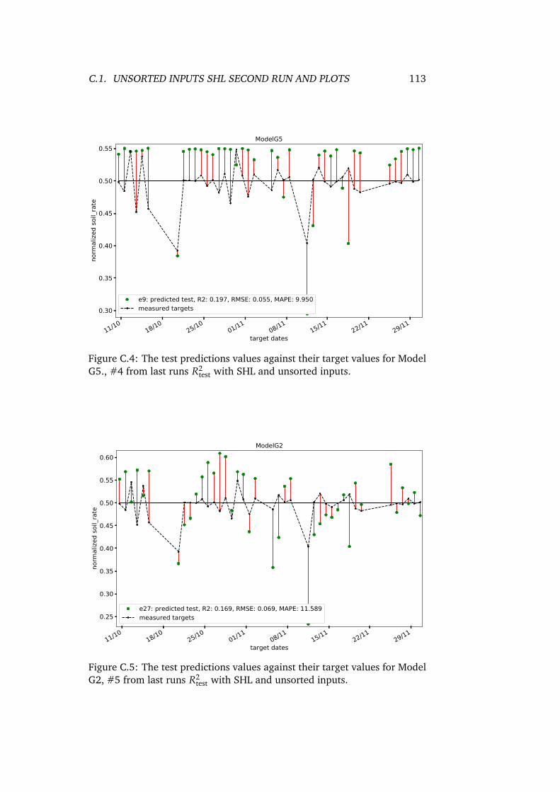
C.1. UNSORTED INPUTS SHL SECOND RUN AND PLOTS 113
11/10
18/10
25/10
01/11
08/11
15/11
22/11
29/11
target dates
0.30
0.35
0.40
0.45
0.50
0.55
norm
alize
d soil_rate
ModelG5
e9: predicted test, R2: 0.197, RMSE: 0.055, MAPE: 9.950measured targets
Figure C.4: The test predictions values against their target values for ModelG5., #4 from last runs R2
test with SHL and unsorted inputs.
11/10
18/10
25/10
01/11
08/11
15/11
22/11
29/11
target dates
0.25
0.30
0.35
0.40
0.45
0.50
0.55
0.60
norm
alize
d soil_rate
ModelG2
e27: predicted test, R2: 0.169, RMSE: 0.069, MAPE: 11.589measured targets
Figure C.5: The test predictions values against their target values for ModelG2, #5 from last runs R2
test with SHL and unsorted inputs.

114 APPENDIX C. ADDITONAL RESULT TABLES AND PLOTS
11/10
18/10
25/10
01/11
08/11
15/11
22/11
29/11
target dates
0.2
0.3
0.4
0.5
0.6
0.7no
rmalize
d soil_rate
ModelD4
e17: predicted test, R2: 0.143, RMSE: 0.101, MAPE: 15.459measured targets
Figure C.6: The test predictions values against their target values for ModelD4, #6 from last runs R2
test with SHL and unsorted inputs.
11/10
18/10
25/10
01/11
08/11
15/11
22/11
29/11
target dates
0.400
0.425
0.450
0.475
0.500
0.525
0.550
0.575
norm
alize
d soil_rate
ModelF3
e3: predicted test, R2: 0.137, RMSE: 0.055, MAPE: 9.479measured targets
Figure C.7: The test predictions values against their target values for ModelF3, #7 from last runs R2
test with SHL and unsorted inputs.

C.1. UNSORTED INPUTS SHL SECOND RUN AND PLOTS 115
11/10
18/10
25/10
01/11
08/11
15/11
22/11
29/11
target dates
0.35
0.40
0.45
0.50
0.55
0.60
norm
alize
d soil_rate
ModelK1e14: predicted test, R2: 0.124, RMSE: 0.064, MAPE: 10.813measured targets
Figure C.8: The test predictions values against their target values for ModelK1, #8 from last runs R2
test with SHL and unsorted inputs.
11/10
18/10
25/10
01/11
08/11
15/11
22/11
29/11
target dates
0.35
0.40
0.45
0.50
0.55
0.60
norm
alize
d so
il_ra
te
ModelE2
e2: predicted test, R2: 0.094, RMSE: 0.061, MAPE: 10.139measured targets
Figure C.9: The test predictions values against their target values for ModelE2, #9 from last runs R2
test with SHL and unsorted inputs.

116 APPENDIX C. ADDITONAL RESULT TABLES AND PLOTS
11/10
18/10
25/10
01/11
08/11
15/11
22/11
29/11
target dates
0.30
0.35
0.40
0.45
0.50
0.55
norm
alize
d soil_rate
ModelG3
e30: predicted test, R2: 0.086, RMSE: 0.044, MAPE: 7.084measured targets
Figure C.10: The test predictions values against their target values for ModelG3, #10 from last runs R2
test with SHL and unsorted inputs.

C.2. SORTED INPUTS SHL PLOTS 117
C.2 Sorted inputs SHL plots

118 APPENDIX C. ADDITONAL RESULT TABLES AND PLOTS
Table C.4: The top 10 best R2 values encountered on the whole dataset forsorted inputs and SHL.
# Model Hiddennodes
epoch R2train R2
test R2 RMSE MAPE
1 ModelG3 13 8 -0.024 0.132 0.032 0.070 11.207
2 ModelI2 9(-5) 6 -0.002 -0.012 0.021 0.139 24.985
3 ModelE3 15(+2) 2 0.017 -0.008 0.018 0.150 26.133
4 ModelD4 7(-5) 3 0.022 0.005 0.015 0.218 38.840
5 ModelD5 11(-1) 1 0.023 0.005 0.015 0.202 35.645
6 ModelF3 9(-4) 3 0.005 0.037 0.009 0.180 34.157
7 ModelD3 15(+3) 18 0.028 0.002 0.009 0.144 23.091
8 ModelI3 17(+3) 2 -0.034 -0.008 0.009 0.200 38.411
9 ModelE5 8(-5) 7 0.022 -0.057 0.009 0.151 23.384
10 ModelG5 13 3 0.016 0.009 0.007 0.215 42.610
Table C.5: The top 10 best R2 values encountered on the train data withsorted inputs and SHL.
# Model Hiddennodes
epoch R2train R2
test R2 RMSE MAPE
1 ModelI5 19(+5) 25 0.062 -0.170 -0.014 0.083 15.190
2 ModelE4 15(+2) 40 0.050 -0.043 0.006 0.161 25.268
3 ModelG4 16(+3) 26 0.037 -0.207 -0.051 0.065 12.405
4 ModelE5 8(-5) 8 0.036 -0.150 0.007 0.118 21.361
5 ModelD5 14(+2) 34 0.034 -0.191 -0.015 0.061 10.357
6 ModelF4 12(-1) 47 0.031 -0.430 -0.032 0.062 10.207
7 ModelD3 15(+3) 18 0.028 0.002 0.009 0.144 23.091
8 ModelF5 13 56 0.025 -1.306 -0.100 0.038 5.394
9 ModelD4 7(-5) 3 0.022 0.005 0.015 0.218 38.840
10 ModelE3 15(+2) 2 0.017 -0.008 0.018 0.150 26.133
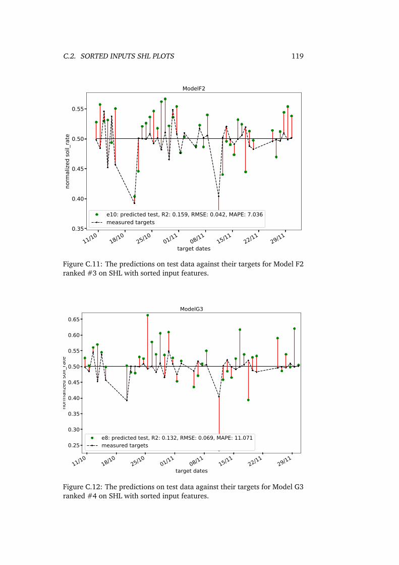
C.2. SORTED INPUTS SHL PLOTS 119
11/10
18/10
25/10
01/11
08/11
15/11
22/11
29/11
target dates
0.35
0.40
0.45
0.50
0.55
norm
alize
d soil_rate
ModelF2
e10: predicted test, R2: 0.159, RMSE: 0.042, MAPE: 7.036measured targets
Figure C.11: The predictions on test data against their targets for Model F2ranked #3 on SHL with sorted input features.
11/10
18/10
25/10
01/11
08/11
15/11
22/11
29/11
target dates
0.25
0.30
0.35
0.40
0.45
0.50
0.55
0.60
0.65
norm
alize
d soil_rate
ModelG3
e8: predicted test, R2: 0.132, RMSE: 0.069, MAPE: 11.071measured targets
Figure C.12: The predictions on test data against their targets for Model G3ranked #4 on SHL with sorted input features.

120 APPENDIX C. ADDITONAL RESULT TABLES AND PLOTS
11/10
18/10
25/10
01/11
08/11
15/11
22/11
29/11
target dates
0.35
0.40
0.45
0.50
0.55no
rmal
ized
soil_
rate
ModelE4
e18: predicted test, R2: 0.130, RMSE: 0.065, MAPE: 11.586measured targets
Figure C.13: The predictions on test data against their targets for Model E4ranked #5 on SHL with sorted input features.
11/10
18/10
25/10
01/11
08/11
15/11
22/11
29/11
target dates
0.35
0.40
0.45
0.50
0.55
0.60
norm
alize
d soil_rate
ModelD4e11: predicted test, R2: 0.127, RMSE: 0.069, MAPE: 11.405measured targets
Figure C.14: The predictions on test data against their targets for Model D4ranked #6 on SHL with sorted input features.
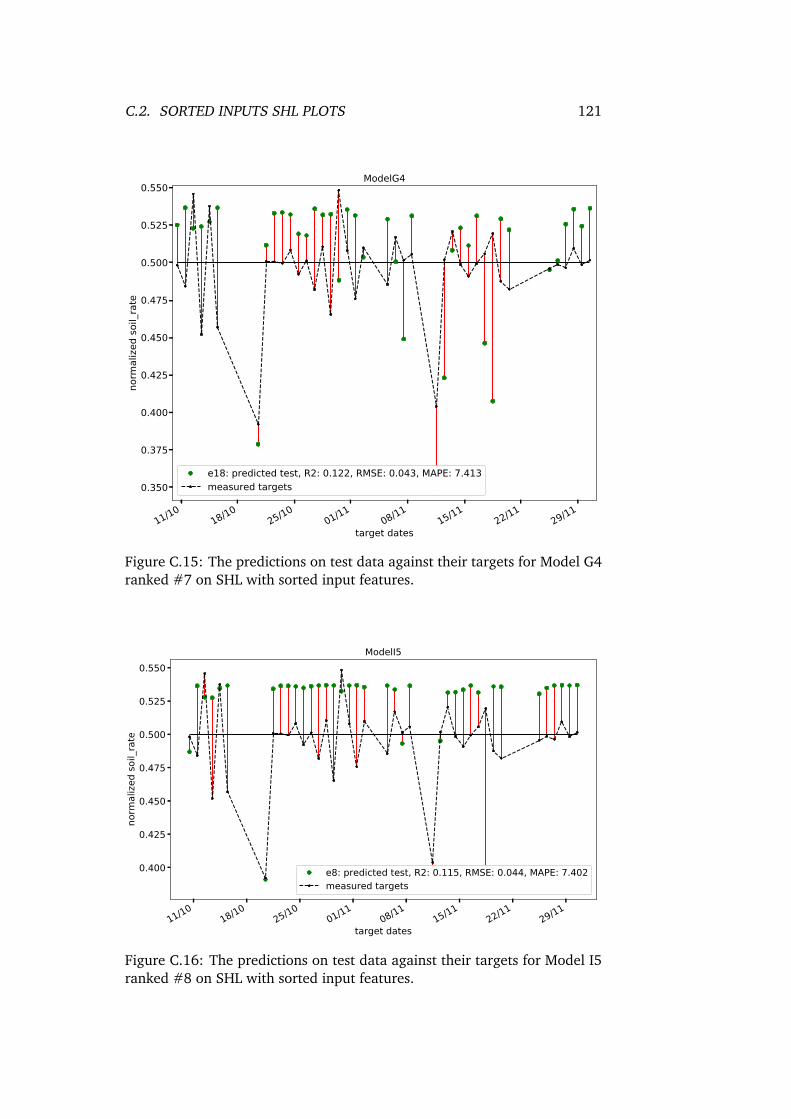
C.2. SORTED INPUTS SHL PLOTS 121
11/10
18/10
25/10
01/11
08/11
15/11
22/11
29/11
target dates
0.350
0.375
0.400
0.425
0.450
0.475
0.500
0.525
0.550
norm
alize
d soil_rate
ModelG4
e18: predicted test, R2: 0.122, RMSE: 0.043, MAPE: 7.413measured targets
Figure C.15: The predictions on test data against their targets for Model G4ranked #7 on SHL with sorted input features.
11/10
18/10
25/10
01/11
08/11
15/11
22/11
29/11
target dates
0.400
0.425
0.450
0.475
0.500
0.525
0.550
norm
alize
d so
il_ra
te
ModelI5
e8: predicted test, R2: 0.115, RMSE: 0.044, MAPE: 7.402measured targets
Figure C.16: The predictions on test data against their targets for Model I5ranked #8 on SHL with sorted input features.

122 APPENDIX C. ADDITONAL RESULT TABLES AND PLOTS
11/10
18/10
25/10
01/11
08/11
15/11
22/11
29/11
target dates
0.40
0.45
0.50
0.55
0.60
norm
alize
d soil_rate
ModelF5e16: predicted test, R2: 0.115, RMSE: 0.064, MAPE: 10.963measured targets
Figure C.17: The predictions on test data against their targets for Model F5ranked #9 on SHL with sorted input features.
11/10
18/10
25/10
01/11
08/11
15/11
22/11
29/11
target dates
0.40
0.42
0.44
0.46
0.48
0.50
0.52
0.54
0.56
norm
alize
d soil_rate
ModelI2e12: predicted test, R2: 0.098, RMSE: 0.033, MAPE: 5.480measured targets
Figure C.18: The predictions on test data against their targets for Model I2ranked #10 on SHL with sorted input features.

C.3. UNSORTED INPUTS DEEP LEARNING SCORES 123
C.3 Unsorted inputs deep learning scores

124 APPENDIX C. ADDITONAL RESULT TABLES AND PLOTS
Table C.6: The top 10 best R2 values encountered on all data of the deeplearning models with unsorted input features.
# Model Hiddennodes
epoch R2train R2
test R2 RMSE MAPE
1 ModelE5 16(+3) 32 0.071 0.019 0.060 0.080 11.837
2 ModelE3 16(+3) 2 0.042 0.009 0.042 0.131 22.301
3 ModelE4 8(-5) 19 0.055 -0.024 0.037 0.127 22.405
4 ModelG4 13 30 0.024 0.069 0.028 0.062 10.276
5 ModelG5 12(-1) 7 0.007 0.080 0.026 0.136 20.752
6 ModelI5 15(+1) 0 0.014 0.009 0.024 0.142 26.228
7 ModelD5 16(+4) 143 0.114 -0.555 0.023 0.051 8.176
8 ModelK4 11(-3) 59 -0.006 0.006 0.022 0.093 15.635
9 ModelK5 12(-2) 26 -0.028 0.030 0.021 0.102 14.576
10 ModelD4 12 7 0.002 0.081 0.019 0.126 23.913

Bibliography
Agboola, AH et al. (2013). “Development of a fuzzy logic based rainfall pre-diction model.” In: International Journal of Engineering and Technology3.4 (cit. on p. 23).
Bayer, Michael (2016). SQLAlchemy. 1.0.1. http://www.sqlalchemy.org/ (cit.on p. 46).
Bonsignore, Luca et al. (2014). “Neuro-Fuzzy Fault Detection Method forPhotovoltaic Systems.” In: Energy Procedia 62, pp. 431–441. ISSN: 1876-6102. DOI: http : / / dx .doi . org /10 .1016 / j . egypro.2014 .12 .405. URL:http://www.sciencedirect.com/science/article/pii/S1876610214034365(cit. on p. 23).
BP (2016). “BP Energy Outlook 2016 edition.” In: URL: /energyoutlook (cit.on p. 1).
Caron, J Riley and Bodo Littmann (2013). “Direct monitoring of energy lostdue to soiling on first solar modules in California.” In: IEEE Journal ofphotovoltaics 3.1, pp. 336–340 (cit. on p. 19).
Dieleman, Sander et al. (2015). Lasagne: First release. DOI: 10.5281/zenodo.27878. URL: http://dx.doi.org/10.5281/zenodo.27878 (cit. on p. 69).
Duchi, John, Elad Hazan, and Yoram Singer (2011). “Adaptive subgradientmethods for online learning and stochastic optimization.” In: Journal ofMachine Learning Research 12.Jul, pp. 2121–2159 (cit. on p. 31).
Energy Yield and Performance Ratio of Photovoltaic Systems (n.d.). http : / /www.greenrhinoenergy.com/solar/technologies/pv_energy_yield.php.Accessed: 2017-04-30 (cit. on pp. 5, 6).
Fraunhofer-ISE (2016). Photovoltaics report. Tech. rep. Fraunhofer Institutefor Solar Energy Systems, ISE (cit. on p. 3).
García, Miguel et al. (2011). “Soiling and other optical losses in solar-tracking PV plants in navarra.” In: Progress in Photovoltaics: Researchand Applications 19.2, pp. 211–217. ISSN: 1099-159X. DOI: 10.1002/pip.1004. URL: http://dx.doi.org/10.1002/pip.1004 (cit. on p. 19).
Gostein, Michael (2014). Update on Edition 2 of IEC 61724: PV SystemPerformance Monitoring. Accessed: 2016-04-30. URL: https://www.nrel.gov/pv/assets/pdfs/2014_pvmrw_84_gostein.pdf (cit. on p. 9).
Guo, B. et al. (2015). “Effect of dust and weather conditions on photovoltaicperformance in Doha, Qatar.” In: 2015 First Workshop on Smart Grid andRenewable Energy (SGRE), pp. 1–6. DOI: 10.1109/SGRE.2015.7208718(cit. on pp. 19, 21).
125

126 BIBLIOGRAPHY
Heaton, Jeff (2015). Neural Networks and Deep Learning. 1.0. Vol. 3.Artificial Intelligence for Humans. Heaton Research, Inc. (cit. on pp. 26,27, 29–31).
IEA. (2015a). “Key world energy statistics.” In: URL: https://www.iea.org/publications/freepublications/publication/key-world-energy-statistics-2015.html (cit. on p. 1).
— (2015b). “World Energy Outlook 2015.” In: DOI: http://dx.doi.org/10.1787/weo-2015-en. URL: /content/book/weo-2015-en (cit. on p. 1).
IEA (n.d.). “World Energy Outlook 2016.” In: DOI: http://dx.doi.org/10.1787/weo-2016-en. URL: /content/book/weo-2016-en (cit. on p. 2).
IEC. (1998). IEC 61724 Std. Photovoltaic System Performance Monitoring-Guidelines for Measurement, Data Exchange and Analysis. IEC. (cit. onp. 9).
ipcc-contributors (2014). Climate Change 2014: Mitigation of ClimateChenge. Report 5. Intergovernmental panel on climate change (cit. onp. 1).
ISO8601 (2000). Data elements and interchange formats – Informationinterchange – Representation of dates and times. Standard 8601:2000.International Organization for Standardization (cit. on p. 52).
Japenga, Robert (2016). How to write a software requirements specification.http://www.microtoolsinc.com/Howsrs.php (cit. on p. 44).
Jones, R. K. et al. (2016). “Optimized Cleaning Cost and Schedule Basedon Observed Soiling Conditions for Photovoltaic Plants in Central SaudiArabia.” In: IEEE Journal of Photovoltaics 6.3, pp. 730–738. ISSN: 2156-3381. DOI: 10.1109/JPHOTOV.2016.2535308 (cit. on p. 4).
Kantardzic, Mehmed (2011). Data mining: concepts, models, methods, andalgorithms. John Wiley & Sons (cit. on pp. 24, 27, 28).
Kingma, Diederik and Jimmy Ba (2014). “Adam: A method for stochasticoptimization.” In: arXiv preprint arXiv:1412.6980 (cit. on p. 32).
Kurokawa, Kosuke et al. (1998). “Sophisticated verification of simplemonitored data for Japanese field test program.” In: KURO LAB. URL:http : / /www.kurochans .net / english / kurochan /e - papers .htm (cit. onp. 11).
LeCun, Yann et al. (1998). “Gradient-based learning applied to documentrecognition.” In: Proceedings of the IEEE 86.11, pp. 2278–2324 (cit. onp. 35).
Lorenz, Elke et al. (2004). “PVSAT-2: Intelligent performance check of PVsystem operation based on satellite data.” In: ResearchGate. URL: https://www.researchgate.net/publication/46658279_PVSAT-2_Intelligent_performance_check_of_PV_system_operation_based_on_satellite_data (cit. on p. 18).
MATLAB Engine API for Python (2016). Accessed: 2017-04-30. MathWorks.http://se.mathworks.com/help/matlab/matlab-engine- for-python.html(cit. on p. 46).
Mejia, Felipe A and Jan Kleissl (2013). “Soiling losses for solar photovoltaicsystems in California.” In: Solar Energy 95, pp. 357–363 (cit. on pp. 4,18).

BIBLIOGRAPHY 127
Micheli, Leonardo and Matthew Muller (2017). “An investigation of the keyparameters for predicting PV soiling losses.” In: Progress in Photovoltaics:Research and Applications 25.4, pp. 291–307 (cit. on p. 97).
Naeem, M. and G. Tamizhmani (2015). “Climatological relevance to thesoiling loss of photovoltaic modules.” In: 2015 Saudi Arabia Smart Grid(SASG), pp. 1–5. DOI: 10.1109/SASG.2015.7449280 (cit. on pp. 4, 19).
Ndapuka, Andreas Tangeni (2015). “Design and development of a monitor-ing station for the long-term investigation of dust pollution effects onthe performance of PV panels.” PhD thesis. Stellenbosch: StellenboschUniversity (cit. on p. 42).
Nouri, Daniel (2014). nolearn: scikit-learn compatible neural network library.URL: https://github.com/dnouri/nolearn (cit. on p. 69).
Plessis, Armand A. du (2016). “The Influence of Dust Soiling on thePerformance of Photovoltaic Modules in the Semi-Arid Areas of SouthAfrica.” MA thesis. University of Stellenbosch (cit. on pp. 21, 39, 40, 52,53, 56).
Pulipaka, Subrahmanyam, Fani Mani, and Rajneesh Kumar (2016). “Mod-eling of soiled PV module with neural networks and regression usingparticle size composition.” In: Solar Energy 123, pp. 116–126 (cit. onp. 24).
PV Modeling Collaborative (2016). URL: https://pvpmc.sandia.gov/ (visitedon 04/30/2016) (cit. on p. 11).
Ramli, Makbul AM et al. (2016). “On the investigation of photovoltaic out-put power reduction due to dust accumulation and weather conditions.”In: Renewable Energy 99, pp. 836–844 (cit. on p. 20).
Al-Rfou, Rami et al. (2016). “Theano: A Python framework for fast compu-tation of mathematical expressions.” In: arXiv e-prints abs/1605.02688.URL: http://arxiv.org/abs/1605.02688 (cit. on p. 69).
Sarver, Travis, Ali Al-Qaraghuli, and Lawrence L. Kazmerski (2013). “Acomprehensive review of the impact of dust on the use of solar energy:History, investigations, results, literature, and mitigation approaches.”In: Renewable and Sustainable Energy Reviews 22, pp. 698–733. ISSN:1364-0321. DOI: http:/ /dx.doi.org/10.1016/j .rser.2012.12.065. URL:http://www.sciencedirect.com/science/article/pii/S136403211300021X(cit. on p. 4).
Serrano-Luján, Lucia et al. (2016). “Case of study: Photovoltaic faultsrecognition method based on data mining techniques.” In: Journal ofRenewable and Sustainable Energy 8.4, p. 043506. DOI: 10 . 1063 / 1 .4960410. eprint: http : / / dx . doi . org / 10 . 1063 / 1 . 4960410. URL: http ://dx.doi.org/10.1063/1.4960410 (cit. on p. 23).
Silvestre, Santiago, Aissa Chouder, and Engin Karatepe (2013). “Automaticfault detection in grid connected {PV} systems.” In: Solar Energy 94,pp. 119–127. ISSN: 0038-092X. DOI: http://dx.doi.org/10.1016/j.solener.2013.05.001. URL: http://www.sciencedirect.com/science/article/pii /S0038092X13001849 (cit. on pp. 15–18).
Spataru, Sergiu et al. (2015). “Diagnostic method for photovoltaic systemsbased on light I–V measurements.” In: Solar Energy 119, pp. 29–44. ISSN:0038-092X. DOI: http://dx.doi.org/10.1016/j.solener.2015.06.020. URL:

128 BIBLIOGRAPHY
www.sciencedirect.com/science/article/pii/S0038092X1500328X (cit.on p. 24).
TC 82 Solar photovoltaic energy systems (61724) (1998). URL: http://www.iec.ch/dyn/www/f?p=103:38:0::::FSP_ORG_ID,FSP_APEX_PAGE,FSP_LANG_ID,FSP_PROJECT:1276,23,25,PNW/TS%5C%2082-1061%5C%20Ed.%5C%201.0# (cit. on p. 9).
Walt, Stéfan van der, Chris Colbert, and Gaël Varoquaux (2011). The NumPyArray: A Structure for Efficient Numerical Computation. [Online; accessed2017-04-21]. DOI: http://dx.doi.org/10.1109/MCSE.2011.37. URL: http://scitation.aip.org/content/aip/journal/cise/13/2/10.1109/MCSE.2011.37(cit. on p. 69).
Weldemariam, Ashenafi (2016). “Analyzing the effect of soiling on theperformance of a photovoltaic system of different module technologiesin Kalkbult, South Africa.” MA thesis. Dalarna University (cit. on p. 41).
Woyte, Achim et al. (2014). IEA-PVPS T13-D2 3 Analytical Monitoring ofPV Systems Final. Tech. rep. International Energy Agency (IEA) (cit. onpp. 9, 10).
Yadav, Amit Kumar and S.S. Chandel (2014). “Solar radiation predictionusing Artificial Neural Network techniques: A review.” In: Renewable andSustainable Energy Reviews 33, pp. 772–781. ISSN: 1364-0321. DOI: http://doi.org/10.1016/j.rser.2013.08.055. URL: http://www.sciencedirect.com/science/article/pii/S1364032113005959 (cit. on p. 24).
— (2017). “Identification of relevant input variables for prediction of 1-minute time-step photovoltaic module power using Artificial NeuralNetwork and Multiple Linear Regression Models.” In: Renewable andSustainable Energy Reviews. ISSN: 1364-0321. DOI: http://dx.doi.org/10.1016/j.rser.2016.12.029. URL: http://www.sciencedirect.com/science/article/pii/S136403211631084X (cit. on pp. 32, 71).
Zorrilla-Casanova, J et al. (2011). “Analysis of dust losses in photovoltaicmodules.” In: World Renewable Energy Congress-Sweden; 8-13 May;2011; Linköping; Sweden. 057. Linköping University Electronic Press,pp. 2985–2992 (cit. on p. 20).
Øgaard, Mari Benedikte (2016). “Effect of Soiling on the Performance ofPhotovoltaic Modules in Kalkbult, South Africa.” MA thesis. Norgesmiljø- og biovitenskaplige universitet (cit. on pp. 20, 21, 42, 52, 58).