1  

 

 

PWT  8.0  –  a  user  guide  

by  

Robert  C.  Feenstra  University  of  California,  Davis  and  NBER  

 Robert  Inklaar  

University  of  Groningen    

Marcel  Timmer  University  of  Groningen  

 April  2013  

 

 

 

 

 

 

 

 

 

 

This  research  received  support  through  NSF  Grant  No.  27-­‐3457-­‐00-­‐0-­‐79-­‐195  for  the   project   entitled   Integrating   Expenditure   and   Production   Estimates   in  International  Comparisons.   Financial   support   from   the  Sloan  Foundation   is  also  gratefully   acknowledged.  We  also   thank  participants   at   the  PWT  workshops   in  Groningen   (2011)   and   Philadelphia   (2012)   and   a   seminar   at   the   Norwegian  School  of  Economics  in  Bergen  for  useful  comments  and  suggestions.  

  2  

Introduction  

The   introduction   of   a   substantially   revised   version   of   the   Penn   World   Table  

(PWT)   is  a  useful  moment   to   introduce  or  reintroduce  this  dataset   to   its  users.  

The  aim  of  this  user  guide  is  to  provide  a  non-­‐technical  overview  of  PWT  version  

8.0:  what   are   the  new   concepts,   how   is   the  dataset   constructed,   how   can   it   be  

best  used  in  research  and  what  are  some  of  the  main  limitations.1    

The  central  element  of  PWT  has  always  been  real  GDP  per  capita,  a  measure  of  

relative   living   standards   across   countries   at   different   points   in   time.   This  

measure   requires   two   main   pieces   of   information,   namely   GDP   per   capita   in  

national   currency   and   purchasing   power   parities   (PPPs)   to   correct   for  

differences   in   prices   across   countries. 2  Many   of   the   choices   necessary   for  

constructing  PWT  are   related   to  estimating  PPPs  and  we  will  use   this  guide   to  

motivate   these   choices   and   discuss   their   consequences.   GDP   data   are   readily  

available   from  National  Accounts   (NA)   statistics,   and   so   require   fewer   choices.  

However,   revisions   of   NA   data   by   statistical   offices   are   often   substantial,   with  

GDP   increasing  by  half   or   even  doubling   in   some   cases.   Such   revisions   are   the  

                                                                                                               

1  For   a  more   technical   discussion   of   the  methodological   innovations   in   PWT  8.0,   see   Feenstra,  

Inklaar   and   Timmer   (2013).   For   discussions   of   earlier   versions,   see   e.g.   Summers   and  Heston  

(1991)  and  Kravis,  Heston  and  Summers  (1982).  

2  A  country’s  PPP  gives  the  number  of  local  currency  units  (e.g.  euro’s)  that  are  needed  to  buy  a  

bundle  of  products  worth  one  dollar   in   the  US.  Dividing   the  PPP  by   the  nominal  exchange  rate  

(also  in  local  currency  units  per  dollar)  then  gives  the  “price  level”  of  that  country  relative  to  the  

US.  A  price  level  of  0.5,   for  example,   indicates  that  local  prices  converted  to  US  dollars  with  the  

nominal  exchange  rate  are  ½  as  high  on  average  as  in  the  United  States,  as  might  be  the  case  for  a  

developing  country.  

  3  

dominant  reason  for  differences  between  subsequent  versions  of  PWT  that  were  

emphasized  by  Johnson  et  al.  (2013).  We  illustrate  this  using  recent  vintages  of  

NA  data.3  

In  version  8.0,  we  make  three  major  changes  to  PWT,  two  of  which  are  related  to  

the   calculation   of   PPPs.   The   first   change   is   that  we   now   also  measure   relative  

prices  of  exports  and  imports.  This  allows  us  to  distinguish  two  measures  of  real  

GDP,  one  aimed  at  capturing  relative  living  standards  (as  before)  and  one  aimed  

at   capturing   relative   productive   capacity.   Researchers   can   thus   choose   the  

measure  that  is  most  appropriate  to  the  research  setting.  The  second  change  is  in  

how  we   estimate   PPPs   over   time,   by   using  more   of   the   historical   price   survey  

material.  This  change  has   important   implications   for  using  PWT  in  research  on  

cross-­‐country  economic  growth.  The  third  change  is  that  we  introduce  measures  

of  capital  stock  and  (total   factor)  productivity,  based  on  newly  developed  basic  

data   discussed   in   Inklaar   and   Timmer   (2013c).   This   broadens   the   type   of  

research   questions   that   can   be   answered   directly   using   PWT,   such   as   models  

relying   on   the   distance   to   the   technological   frontier   (e.g.   Aghion   and   Howitt,  

2006).   Here   we   discuss   these   changes   in   broad   terms   and   focus   on   the  

implications  of  our  choices.  

The  limitations  inherent  in  comparing  living  standards  or  productive  capacity  of  

economies  across  countries  are  a  recurring  theme  in  this  guide.  Whether  due  to  

the  very  nature  of  the  exercise  or  the  practical  challenges  encountered  along  the  

                                                                                                               

3  GDP  per  capita  data  also  requires  data  on  the  population  of  a  country.  Such  data  is  typically  less  

prone  to  large  revisions.  

  4  

way,  it  is  not  possible  to  be  very  precise  in  comparing  countries  at  very  different  

levels   of   economic   development;   see   also   Deaton   and   Heston   (2010).   Beyond  

that,   changing   basic   national   accounts   data   can   and   will   lead   to   substantial  

differences  in  PWT  versions  over  time.  In  response  to  the  work  of  Johnson  et  al.  

(2013),   we   have   changed   the   PWT   methodology   to   reduce   the   likelihood   of  

revisions   over   time,   but   a   complete   elimination   of   this   concern   is   impossible  

because  of  changes  to  the  underlying  data.  This   implies  that  caution  is   in  order  

when  using  the  reported  results  and  we  discuss  when  to  be  cautious  and  provide  

practical  suggestions  on  how  to  be  cautious.  

These  recommendations  will  not  apply  to  the  same  degree  to  every  user  and  we  

will   clarify   this   throughout.   In   general,   users   that   are   interested   in   specific  

numbers,   such   as   the   relative   price   level   of   Tanzania   in   2000   or   the   GDP   per  

capita  ranking  of  Vietnam  in  1995,  will  need  to  be  most  careful  as  limitations  to  

the  basic  data  and  specific  methodological  choices  have  their   largest   impact  on  

such  individual  observations.  These  would  typically  be  most  relevant  for  the  type  

of   analysis   done   in   country-­‐level   studies,   such   as   OECD   Economic   Surveys.   If  

instead  an  econometric   analysis   is  performed  on  a  dataset  based  on  PPPs   (e.g.  

Rodrik,  2008)  or  real  GDP  per  capita  levels  (e.g.  Ashraf  and  Galor,  2013),  some  of  

these  considerations  may  be   less   important  as   the  broad  cross-­‐country  pattern  

of  data  is  not  severely  affected  by  some  of  these  choices.  Finally,  for  those  aiming  

to   explain   differences   in   cross-­‐country   economic   growth,  while   accounting   for  

differences  in  initial  real  GDP  per  capita  levels,  the  recommendations  for  when  to  

use  real  GDP  per  capita  and  when  to  use  GDP  at  constant  national  prices  will  be  

most  relevant.    

  5  

GDP  per  capita  –  a  numerical  example  

To   illustrate   the  main  concepts   fromPWT8.0,  Table  1  compares  GDP  per  capita  

and   productivity   in   China   and   the   United   States   in   2005.   The   first   row   shows  

GDP   per   capita   in   national   currency,   so   in   renminbi   (RMB)   for   China   and   US  

dollars   (USD)   for   the   US,   and   these   data   are   directly   from   National   Accounts.  

Since  these  values  are  in  different  currencies,  a  comparison  between  the  Chinese  

and  US  values  makes  little  sense.  The  second  row  converts  the  Chinese  value  in  

US   dollars   using   the   market   exchange   rate   at   the   time   of   8.2   RMB/USD.  

Comparing  the  Chinese  and  US  values  implies  that  China’s  GDP  per  capita  level  is  

only   4   percent   of   that   in   the   US.   However,   the  market   exchange   rate   will   not  

reflect   relative  prices  of  non-­‐traded  products,   such  as  housing  and  many  other  

services,   while   a   PPP   is   designed   to   compare   prices   for   all   products   in   the  

economy.  The  third  row  shows  the  so-­‐called  GDPe  per  capita   from  PWT8.0  and  

this   makes   a   considerable   difference,   with   China’s   relative   income   level   at   12  

rather  than  4  percent  of  that  in  the  US.  As  will  be  discussed  in  more  detail  below,  

GDPe  per  capita  is  a  measure  of  comparative  living  standards  as  it  covers  prices  

for  consumption  and  investment  but  not  for  exports  or  imports.  As  a  result,  the  

value  for  the  United  States  is  also  affected  (43209  vs.  42330).  Row  4  shows  GDPo  

per   capita,   which   does   reflect   relative   prices   of   exports   and   imports   and   is  

thereby   a   measure   of   comparative   productive   capacity.   China   has   the   same  

comparative  living  standards  and  productive  capacity  relative  to  the  US,  but  this  

is  not  true  in  general,  as  we  will  demonstrate  below.  

  6  

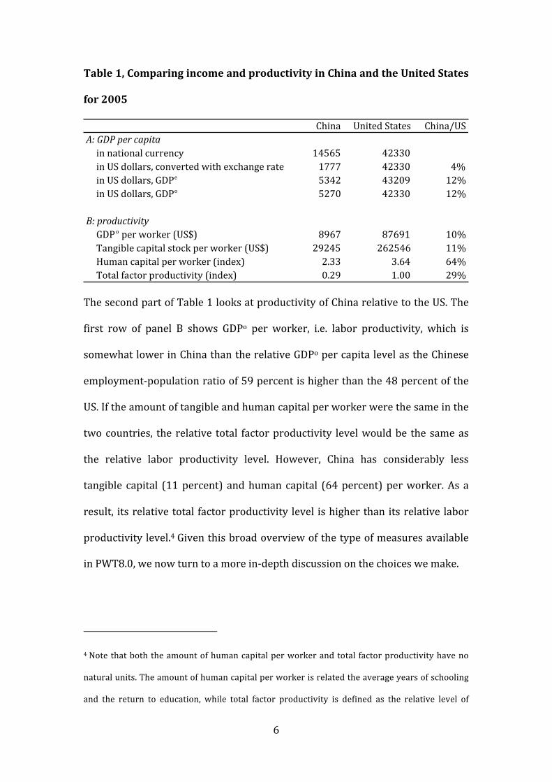
Table  1,  Comparing  income  and  productivity  in  China  and  the  United  States  

for  2005  

 

The  second  part  of  Table  1  looks  at  productivity  of  China  relative  to  the  US.  The  

first   row   of   panel   B   shows   GDPo   per   worker,   i.e.   labor   productivity,   which   is  

somewhat  lower  in  China  than  the  relative  GDPo  per  capita  level  as  the  Chinese  

employment-­‐population  ratio  of  59  percent  is  higher  than  the  48  percent  of  the  

US.  If  the  amount  of  tangible  and  human  capital  per  worker  were  the  same  in  the  

two  countries,   the   relative   total   factor  productivity   level  would  be   the  same  as  

the   relative   labor   productivity   level.   However,   China   has   considerably   less  

tangible   capital   (11  percent)   and  human   capital   (64  percent)  per  worker.  As   a  

result,   its  relative  total   factor  productivity   level   is  higher  than  its  relative   labor  

productivity  level.4  Given  this  broad  overview  of  the  type  of  measures  available  

in  PWT8.0,  we  now  turn  to  a  more  in-­‐depth  discussion  on  the  choices  we  make.  

                                                                                                               

4  Note   that  both  the  amount  of  human  capital  per  worker  and  total   factor  productivity  have  no  

natural  units.  The  amount  of  human  capital  per  worker  is  related  the  average  years  of  schooling  

and   the   return   to   education,   while   total   factor   productivity   is   defined   as   the   relative   level   of  

China United*States China/USA:#GDP#per#capitain*national*currency 14565 42330in*US*dollars,*converted*with*exchange*rate 1777 42330 4%in*US*dollars,*GDPe 5342 43209 12%in*US*dollars,*GDPo 5270 42330 12%

B:#productivityGDPo*per*worker*(US$) 8967 87691 10%Tangible*capital*stock*per*worker*(US$) 29245 262546 11%Human*capital*per*worker*(index) 2.33 3.64 64%Total*factor*productivity*(index) 0.29 1.00 29%

  7  

PPPs  for  consumption  and  investment  

Comparing  GDP  levels  across  countries  requires  correcting  for  price  differences  

across   countries.   This   challenge   is   analogous   to   measuring   GDP   growth   over  

time:  knowing   the  change   in   the  quantity  of  products  produced   in  an  economy  

requires  correcting  (nominal)  values  for  changes  in  prices.  But  while  measuring  

price   changes   over   time   is   a  well-­‐understood   and   (mostly)   routine   part   of   the  

work  of  statistical  offices  around  the  world,  measuring  price  differences  across  

countries  is  much  more  of  a  challenge.  This  is  because  spending  patterns  tend  to  

be   very   different,   especially  when   comparing   rich   and   poor   countries,   see   e.g.  

Deaton  and  Heston  (2010).  For  instance,  people  in  poor  countries  tend  to  spend  

much  more  of  their  income  on  food  (Almås,  2012),  so  that  food  prices  are  much  

more   important   for   living   standards   than   in   rich   countries.   An   estimate   of  

relative   living   standards   needs   to   take   both   sets   of   spending   patterns   into  

account,   which   is   an   inherently   imperfect   endeavor.5  A   challenge   of   a   more  

practical  nature  is  how  to  compare,  say,  the  cost  of  housing  in  a  Nairobi  slum  to  

that  in  a  Washington,  DC  suburb.  Even  if  one  can  measure  how  much  is  spent  on  

housing  in  the  two  places,  determining  how  much  of  the  difference  in  spending  is  

due  to  price  differences  and  how  much  due  to  the  difference  in  the  ‘quantity’  of  

                                                                                                                                                                                                                                                                                                                             

output  divided  by  the  relative  level  of  inputs.  In  both  cases,  there  is  no  natural  interpretation  of  

the  absolute  values,  only  of  the  relative  values.  

5  Deaton   and   Heston   (2010)   discuss   this   problem   and   provide   an   introduction   to   the   broader  

index   number   literature.   Note   that   these   differences   in   spending   patterns   can   be   the   result   of  

differences  in  prices,  but  also  of  differences  in  preferences  and  that  taking  such  differences  into  

account  is  still  challenging  (Neary,  2004).    

  8  

housing  is  even  harder.  As  a  result,  the  PPP  comparing  prices  in  Canada  to  the  US  

will  be  much  more  precisely  estimated  than  the  PPP  for  Kenya  relative  to  the  US.  

In  2005,   the  World  Bank’s   International  Comparisons  Program   (ICP)  made   the  

most   recent   benchmark   comparison   of   consumption   and   investment   prices  

based   on   a   detailed   cross-­‐country   price   survey   covering   146   countries   around  

the   world   (see   World   Bank,   2008).   More   recently,   a   broad   review   of   this  

comparison  appeared  (World  Bank,  2013),  which  provides  “health  warnings”  as  

well  as  suggestions  for  the  next  global  comparison,  of  prices  in  2011  across  200  

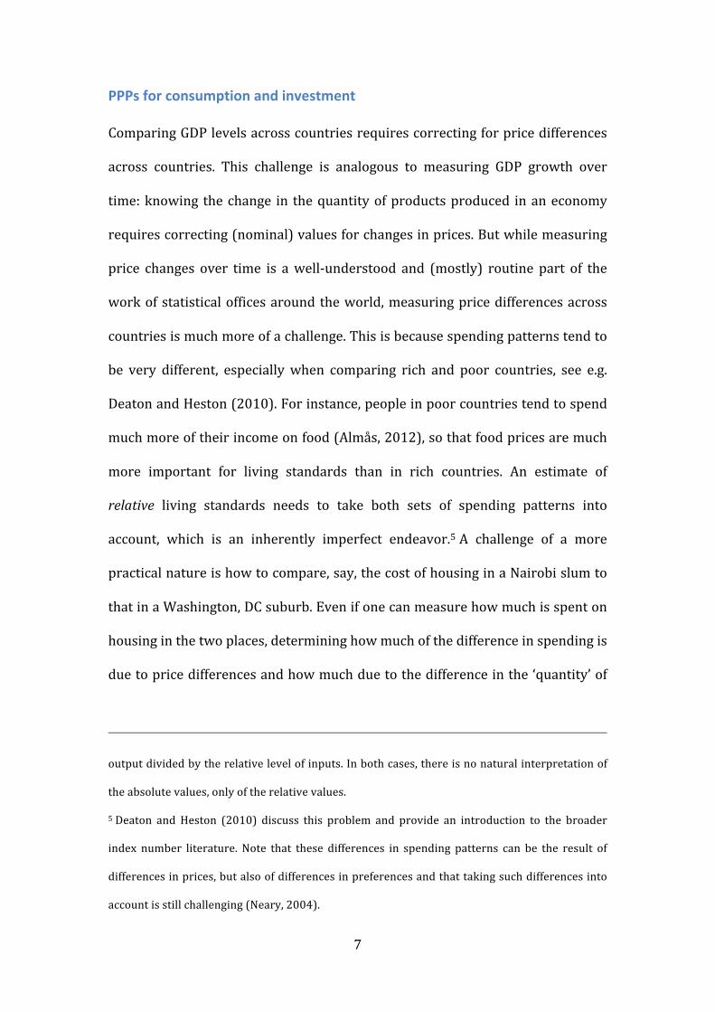
countries.  The  2005  comparison  was  a  great   improvement  over  the   five  earlier  

global   comparisons.   Most   notably,   it   covered   the   largest   number   of   countries  

ever   as   shown   in   Table   2,   and   the   data   collection,   processing   and   PPP  

computation  were  also  more  rigorous.  The  table  also  illustrates  that  before  1996,  

European  countries  and  OECD  countries  elsewhere  made  up  the   lion’s  share  of  

countries.   Country   coverage   in  most   other   regions   has   steadily   risen,  with   the  

exception  of  Latin  America,  where  coverage  has  fluctuated  over  the  years.  

Table  2,   ICP  global  benchmark  comparisons  and  country  participation,  by  

region  

 

*  The  1996  benchmark  was  constructed   for  PWT6  based  on   the  1996  survey   for  OECD  and  EU  

countries  and  the  1993  survey  for  other  regions  in  the  world.  

ICP$benchmark 1970 1975 1980 1985 1996* 2005Europe$&$OECD 10 18 22 25 31 44Asia 3 6 6 8 12 22Latin$America 1 4 16 7 21 10Middle$East$&$North$Africa 1 2 3 4 12 15SubKSaharan$Africa 1 3 13 19 19 45Former$Soviet$Union$(CIS) 12 10Total 16 33 60 63 107 146

  9  

This   discussion   illustrates   the   main   features   and   limitations   of   the   PPP  

information  used   in  PWT:  data   is  available   for   relatively   few  benchmark  years,  

for  an   incomplete  set  of  countries,  and  data  quality  varies  across  countries  and  

years.  As  the  aim  of  PWT  is  to  provide  a  broad  and  complete  panel  of  real  GDP  

estimates,  the  PPP  source  material  requires  further  choices  and  estimation.  The  

first  set  of  choices  is  on  how  to  use  the  basic  benchmark  material;  the  second  on  

dealing  with  non-­‐benchmark  countries  and  years.  

Benchmark  comparisons  

In  each  of  the  six  global  comparisons,  prices  are  collected  for  many  consumption  

and   investment   products.   Together,   these   cover   all   of   domestic   absorption,   i.e.  

GDP  excluding  the  trade  balance;  comparing  the  trade  balance,  i.e.  exports  minus  

imports,   across   countries  will   be   discussed   in  more   detail   in   the   next   section.  

Price  quotes  would  be  collected  on,  for  example,  rice  of  different  types  and  sold  

in  different  package  sizes  and  the  resulting  relative  prices  are  then  averaged  to  

arrive  at  a  relative  price  of  rice.  Overall,  a  list  of  roughly  1000  products  is  priced  

in   every   country   to   cover   all   of   consumption  and   investment.  These  prices   are  

combined   into   100   or  more   so-­‐called   basic   headings   for   which   information   is  

available  about  the  expenditure  on  these  products.6  We  mostly  take  these  basic  

heading  prices  and  expenditures  as  given,  though  for  the  2005  benchmark,  two  

adjustments  were  made.   First,   the   relative   consumption   prices   for   China  were  

deemed  20  percent   too  high  by  Deaton  and  Heston  (2010),   so  all   consumption  

                                                                                                               

6  The   exception   is   the   1996   global   comparison,   for   which   only   about   30   basic   headings   are  

available.  

  10  

basic  headings  were  adjusted  downwards  by  this  proportion.7  Second,  for  much  

of   government   consumption   (health,   education,   collective   services),   no   relative  

output   prices   are   available,   so   instead   relative   input   prices   –   mostly   relative  

wages  –  are  used.  Since  there  are  large  productivity  differences  across  countries,  

these   relative   input   prices   are   a   poor   predictor   of   relative   output   prices.8  The  

World  Bank  (2008)  made  an  adjustment  for  some  countries,  but  Heston  (2013)  

discusses  a  method  to  make  an  adjustment   for  all  countries  and  this  method   is  

applied  in  both  PWT7.x  and  8.0.  

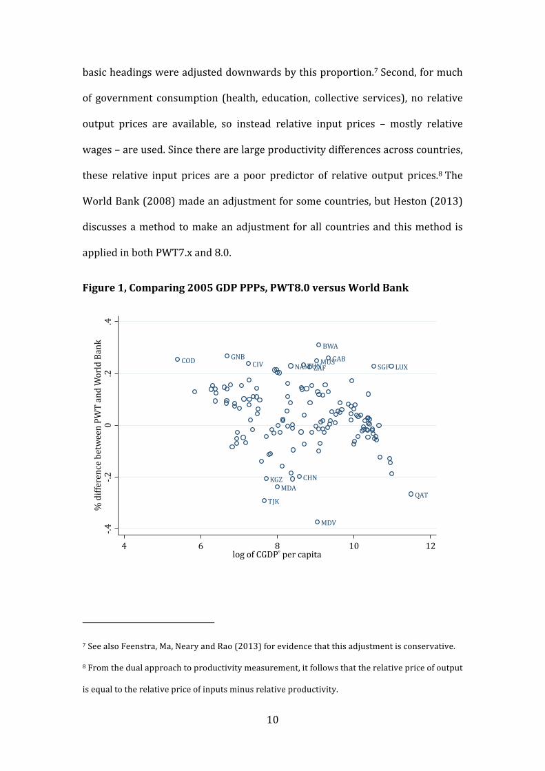
Figure  1,  Comparing  2005  GDP  PPPs,  PWT8.0  versus  World  Bank  

 

                                                                                                               

7  See  also  Feenstra,  Ma,  Neary  and  Rao  (2013)  for  evidence  that  this  adjustment  is  conservative.  

8  From  the  dual  approach  to  productivity  measurement,  it  follows  that  the  relative  price  of  output  

is  equal  to  the  relative  price  of  inputs  minus  relative  productivity.  

BWA

CHN

CIVCOD GABGNB

KGZ

LUX

MDA

MDV

MUSNAM

QAT

SGP

TJK

TUNZAF

8.48.2

0.2

.4%>difference>between>PW

T>and>World>Bank

4 6 8 10 12log>of>CGDPQ>per>capita

  11  

Note:  the  PWT8.0  PPP  refers  to  the  GDPo  PPP,  the  World  Bank  GDP  PPP  is  taken  from  World  Bank  

(2008).  

The  next  step  is  to  compute  a  weighted  average  of  basic  heading  PPPs  to  arrive  

at  an  overall  GDP  PPP.  There  are  a   large  number  of   index  number  methods   for  

doing   so,   and   each   of   these   corresponds   to   a   different   approach   to   weighting  

individual  basic  heading  PPPs.  A  detailed  comparison  of  these  methods  is  beyond  

the   scope  of   this  paper,9  but  all   aim   to  give   larger  weight   to   those  products  on  

which  an  economy  spends  relatively  more.  Here  too,  PWT  version  8.0  will  follow  

somewhat  different  procedures   than   the  World  Bank,   including  different   index  

number  methods10;   different   treatment   of   regional   data;11  and   a   different   PPP  

conversion   of   the   trade   balance;12  see  World   Bank   (2008)   for   details   on   their  

approach  and  Feenstra  et  al.  (2013)  for  details  on  PWT.  These  factors,  together  

with   the   changes   to   the  basic  headings   for  China  and   for   government   services,  

explain  why  PWT  GDP  PPPs   in  2005  are  different   than   the  World  Bank  (2008)  

PPPs.  Figure  1  plots  these  differences  against  the  real  GDP  per  capita  level  from  

PWT8.0.  This  shows  how  differences  are  often  substantial  and  these  occur  at  all  

                                                                                                               

9  For  those  interested,  see  e.g.  Diewert  (2013)  or  Balk  (2008).  

10  The  World  Bank   (2008)  uses   the  GEKS  procedure   in  most   regions  and   the   IDB  procedure   in  

Africa,  while  PWT  uses   the  GEKS  procedure   to  go   from  the  basic  heading   level   to  consumption  

and  investment  and  the  GK  procedure  to  combine  these  to  total  GDP.  

11  The  World  Bank’s  methods  maintains  fixed  parities  within  regions,  also  when  computing  PPPs  

across  regions,  while  in  PWT  this  is  only  the  case  for  EU/OECD  countries,  whose  benchmark  PPP  

data  come  directly  from  Eurostat  and  OECD.  

12  The  World   Bank   uses   the   exchange   rate   to   convert   the   trade   balance,  while   PWT  measures  

specific  PPPs  for  exports  and  imports;  see  the  next  section  for  details.  

  12  

levels   of   income.   This   will   obviously   be   important   for   users   interested   in   the  

income  level  of  specific  countries,  though  for  users  interested  only  in  the  broad  

cross-­‐country   pattern,   the   cross-­‐country   correlation   of   0.97   between   the   two  

sets  of  PPPs  should  be  reassuring.  

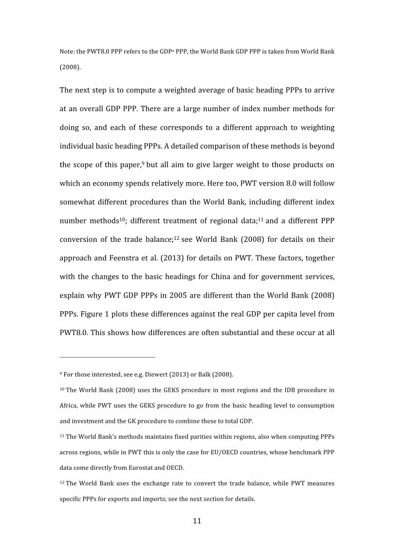
Figure  2,  Correlation  between  expenditure  shares  of  each  country  and  the  

US  across  benchmark  comparisons  compared  with   income  levels  and  PPP  

precision  

 

Note:  difference  between  alternative  PPP   indexes   is   the  percent  difference  between  a  GDP  PPP  

computed  using  the  GEKS  index  number  and  the  Geary-­‐Khamis  (GK)  index  number.  

As   discussed   above,   some   of   the   differences   seen   in   Figure   1   are   due   to  

differences   in   index  number  methods.  The  choice  of   index  number  method  will  

matter   more   when   comparing   two   countries   with   very   different   spending  

patterns.  Since  the   literature  has  advanced  many  plausible  alternative  methods  

and  has  proven  that  none  of  these  will  be  perfectly  suited  to  the  job  (Van  Veelen,  

0.2

.4.6

.81

4 6 8 10 12log+of+GDPe+per+capita

0.2

.4.6

.81

7.6 7.4 7.2 0 .2Difference+between+alternative+PPP+indexes

  13  

2002),  there  will  be  a  margin  of  uncertainty  in  every  cross-­‐country  comparison  

of   prices   and   real   income.   Furthermore,   that   uncertainty   will   be   larger   when  

comparing  countries  for  which  spending  patterns  differ  more.  

Since   information   on   those   spending   patterns   is   available,   we   compute   the  

correlation   between   each   country’s   expenditure   shares   and   those   in   the   US.13  

The   left-­‐hand  panel   of   Figure  2  plots   these   correlations   against   the   log  of  GDP  

per   capita   for   each   of   the   six   global   comparisons.   As   expected,   expenditure  

shares  in  rich  countries  are  more  similar  to  those  in  the  US  than  shares  in  poor  

countries.  If  the  aim  is  to  compare  each  country’s  income  level  to  that  in  the  US,  

then   this   correlation  measure  suggests   that   richer  countries’   income   levels   can  

be   more   precisely   estimated   than   poorer   countries’   income   levels.   The   right-­‐

hand  panel  plots   these  correlations  against   the  percent  difference   in  GDP  PPPs  

across  two  popular  index  number  methods,  the  GEKS  and  the  Geary-­‐Khamis  (GK)  

methods. 14  This   shows   that   for   countries   with   more   highly   correlated  

expenditure  patterns,   the  choice  of  PPP  method  matters   less  than  for  countries  

with  much  lower  correlations.  To  illustrate:  if  the  correlation  is  0.7  or  higher,  the  

average   absolute   difference   between   the   two   PPPs   is   only   4.5   percent;   if   it   is  

lower  than  0.7,  the  difference  is  almost  15  percent.  More  in  general,  the  fact  that  

                                                                                                               

13  The  correlation  of  expenditure  shares  is  chosen  as  it  is  an  intuitive  measure  that  is  related  to  

the   computation   of   PPPs.   For   a  more   rigorous   discussion   on   similarity  measures,   see   Diewert  

(2002).  

14  See  e.g.  Diewert  (2013)  or  Balk  (2008)  for  more  details  on  these  methods.  The  GK  method  has  

traditionally   been   used   in   PWT,   while   the   GEKS   method   has   gained   ground   in   the   statistical  

community.  PWT8.0  uses  a  combination  of  these  methods,  see  below  for  details.  

  14  

the  difference   in  PPPs  according  to   two  widely-­‐used  method  can  be  as   large  as  

50  percent  illustrates  that  due  care  is  needed  when  comparing  living  standards  

between  rich  and  poor  countries.    

In   PWT8.0,   we   provide   the   correlation   between   expenditure   shares   in   each  

country   and   the   US   for   all   benchmark   observations.   In   addition,  we   provide   a  

separate  file  with  all  the  bilateral  correlations,  as  those  will  be  more  useful  when  

comparing,   say,   China   and   India,   rather   than   India   and   the   US.   While   the  

correlations  are  not  a  structural  measure  of  the  reliability  of  PPP  estimates,  they  

can  be  used   as   a  warning   signal   that  whenever   the   correlation   is   low,   the   real  

GDP   (per   capita)   level   should   not   be   interpreted   with   too   much   precision.15  

Furthermore,  we  provide   the  software  so   that  alternative  PWT  datasets  can  be  

constructed  using  different  PPP  methods,  so  that  for  any  set  of  empirical  results  

the  sensitivity  to  this  choice  can  be  assessed.  

The  discussion  so  far  has  focused  on  PPP  data  from  the  global  ICP  comparisons.  

In  addition  to  these,  Eurostat  and  the  OECD  also  collect  and  estimate  PPP  data,  

see  Eurostat/OECD   (2012).   These   comparisons   are  done  more   frequently   than  

the   ICP   comparisons,   annually   since   1995   for   countries   covered   by   Eurostat  

(current   and   potential   future   EU   members)   and   once   every   three   years   since  

1996  for  (other)  OECD  countries.  Assuming  that  any  benchmark  PPP  observation  

                                                                                                               

15  One   alternative   approach   would   be   to   estimate   PPPs   in   country-­‐product-­‐dummy   (CPD)  

regression   as   in   Rao   (2005)   and   use   the   standard   errors   of   the   coefficients   as   a   reliability  

measure.   However,   such   a   measure   ignores   the   variation   in   expenditure   shares   and   only  

accounts   for  the  variation  in  relative  prices  across  products.  That  variation  is  unrelated  to  GDP  

per  capita  or  the  correlation  of  expenditure  shares  measure.  

  15  

leads  to  a  more  reliable  estimate  of  real  GDP  than  a  non-­‐benchmark  observation  

–on   which   more   below–   it   is   very   useful   to   incorporate   such   additional  

benchmark  data,  so  that  is  what  we  do  in  PWT8.0.  

Non-­‐benchmark  countries  

Combining  PPP  data  from  the  six  global  ICP  comparisons  and  the  OECD/Eurostat  

comparisons  only  provides  data  for  a  modest  number  of  countries  and  years,  436  

observations   from   ICP   and   438   from   OECD/Eurostat.   Furthermore,   only   167  

countries  have  at  some  point  participated  in  an  ICP  comparison.  Compare  this  to  

the   209   countries   or   areas   for  which   the  UN  National  Accounts   (NA)   compiles  

GDP   data   and   there   is   a   clear   shortfall.   This   shortfall   is   even   larger   when  

comparing  the  number  of  country-­‐year  observations:  from  UN  NA  and  historical  

NA   data,   we   have   a   dataset   of   10105   observations   spanning   the   period   from  

1950   to   2011.   This  means   that   PPP   benchmark   data   are   directly   available   for  

only   8.6   percent   of   all   country-­‐year   observations.   Furthermore,  many   of   these  

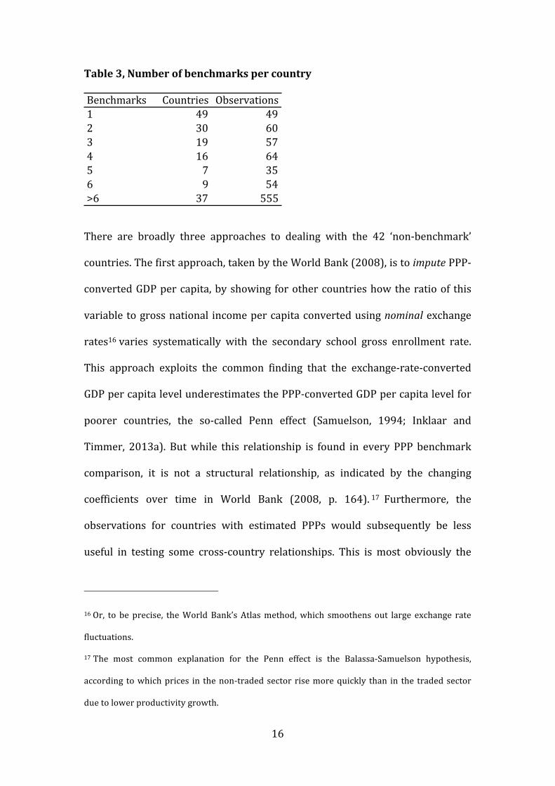
benchmark   observations   are   for   a   limited  number   of   countries.   Table   3   shows  

that   49   countries   only   participated   in   a   single   benchmark   comparisons,   while  

only  37  (European  and  OECD)  countries  participated  in  more  than  6  benchmarks.  

How   then   to  deal  with   the  42   countries   that  have  never  participated   in  an   ICP  

comparison   and   how   to   deal   with   the   many   years   for   which   there   are   no  

benchmark  PPP  observations  for  the  other  167  countries?  

  16  

Table  3,  Number  of  benchmarks  per  country  

 

There   are   broadly   three   approaches   to   dealing   with   the   42   ‘non-­‐benchmark’  

countries.  The  first  approach,  taken  by  the  World  Bank  (2008),  is  to  impute  PPP-­‐

converted  GDP  per  capita,  by  showing   for  other  countries  how  the  ratio  of   this  

variable  to  gross  national   income  per  capita  converted  using  nominal  exchange  

rates16  varies   systematically   with   the   secondary   school   gross   enrollment   rate.  

This   approach   exploits   the   common   finding   that   the   exchange-­‐rate-­‐converted  

GDP  per  capita  level  underestimates  the  PPP-­‐converted  GDP  per  capita  level  for  

poorer   countries,   the   so-­‐called   Penn   effect   (Samuelson,   1994;   Inklaar   and  

Timmer,   2013a).   But  while   this   relationship   is   found   in   every   PPP   benchmark  

comparison,   it   is   not   a   structural   relationship,   as   indicated   by   the   changing  

coefficients   over   time   in   World   Bank   (2008,   p.   164). 17  Furthermore,   the  

observations   for   countries   with   estimated   PPPs   would   subsequently   be   less  

useful   in   testing   some   cross-­‐country   relationships.   This   is   most   obviously   the  

                                                                                                               

16  Or,   to   be   precise,   the  World  Bank’s  Atlas  method,  which   smoothens   out   large   exchange   rate  

fluctuations.  

17  The   most   common   explanation   for   the   Penn   effect   is   the   Balassa-­‐Samuelson   hypothesis,  

according   to  which  prices   in   the  non-­‐traded  sector   rise  more  quickly   than   in   the   traded  sector  

due  to  lower  productivity  growth.  

Benchmarks Countries Observations1 49 492 30 603 19 574 16 645 7 356 9 54>6 37 555

  17  

case  for  testing  the  Penn  effect  (which  was  assumed  when  imputing  the  PPPs  for  

missing  countries),  but  could  be  a  broader  problem  as  well.  

The   second   approach,   taken   in   earlier   versions   of   PWT,   is   to   use   ‘post-­‐

adjustment’   indices.   These   are   indices   used   by,   for   instance,   the   UN   or   the   US  

State   Department   to   determine   the   cost   of   living  when   expats   are   posted   in   a  

foreign  (capital)  city.  This  approach  does  not  suffer  from  the  problem  of  the  first  

approach,   namely   that   the   estimated   PPPs   would   already   reflect   some   of   the  

cross-­‐country   patterns   one   may   wish   to   test.   However,   it   is   unclear   to   which  

degree   these   indices   reflect   the   same   information   as   PPPs,   or   even   the   same  

information   as   each   other.   The   three   sets   of   post-­‐adjustment   indices   used   in  

PWT6.1   show  very  extensive  differences   for  numerous   countries.  For  example,  

according  to  the  UN  index,  prices  in  Myanmar  are  15  percent  lower  than  in  the  

US,  while   the   index   from  Employment   Conditions  Abroad   indicates   that   prices  

are  almost  50  percent  higher.  The  same  range  of  estimates  can  also  be  found  for  

rich   countries,   such   as   the  UK.   So  while   there  may  be   a   statistical   relationship  

between  PPPs  and  post-­‐adjustment  indices,  it  is  hard  to  determine  how  far  such  

a  relationship  can  be  trusted.  

Both  of  these  approaches  have  two  further  (mostly  practical)  drawbacks.  First  of  

all,  to  deal  with  non-­‐benchmark  years  we  use  relative  prices  for  components  of  

GDP,   rather   than   GDP   as   a   whole   –   see   below   for   details.   Even   if   these   two  

approaches   would   be   useful   for   estimating   economy-­‐wide   price   levels,  

estimation  for  the  GDP  components  would  be  required  to  fully  incorporate  these  

non-­‐benchmark  countries  into  PWT.  The  second,  and  related,  drawback  is  a  loss  

of   transparency.  Because  one  or  more  additional   estimations  would  be  needed  

  18  

for  some  countries  but  not  for  others,  we  believe  it  would  make  PWT  harder  to  

interpret.  

We  have   therefore  opted   for  a   third  approach,  namely   to  omit   these  countries.  

This  is  not  ideal,  as  it  means  a  less  rich  dataset.  However,  less  than  3  percent  of  

the   world   population   live   in   non-­‐benchmark   countries.   Of   these,   Myanmar,  

Algeria,  Afghanistan  and  North  Korea  already  account  for  two-­‐thirds  of  the  non-­‐

benchmark   population.   Omitting   non-­‐benchmark   would   thus   not   lead   to   a  

distorted   view   of   global   economic   performance.   Furthermore,   with   the   even  

greater  country  coverage  of  ICP  2011,  the  category  of  non-­‐benchmark  countries  

is   set   to   shrink   even   further.   PWT8.0  will   thus   only   include   the   167   countries  

that  participated  in  a  global  ICP  price  comparison  at  some  point  in  the  past.  

Non-­‐benchmark  years  

That  still   leaves  the  majority  of  country-­‐year  observations  that  are  not  covered  

by  PPP  benchmarks.  Estimating  PPPs  for  non-­‐benchmark  years  will  typically  rely  

on   data   on   national   price   changes.   If   a   PPP   is   the   price   of   goods   in   country   A  

relative   to   those   in   country   B,   then   the   change   in   this   PPP   may   be   well  

approximated   by   the   change   in   prices   in   country   A   relative   to   the   change   in  

prices   in   country   B.   This   will   hold   by   definition   when   comparing   prices   of  

individual  products,  but  comparing  the  relative  price  of  a  bundle  of  goods  is  more  

complicated.    

This   problem   arises,   again,   because   spending   patterns   differ   across   countries  

and  over  time,  but  also  because  prices   for  different  product  change  at  different  

rates  over  time  and  across  countries.  Statisticians  compiling  the  consumer  price  

index   (CPI)   only   have   to   take   into   account   price   changes   and   the   national  

  19  

spending  pattern.  But  when  compiling  a  PPP,  all  sets  of  budget  shares  have  to  be  

taken   into  account,   for   instance  by  using   the  average  share   to  weight   the  price  

difference  for  each  product.18  As  shown  by  Deaton  (2012),  this  is  likely  to  lead  to  

systematic  differences  between  national   inflation  rates  and  the  change  in  PPPs,  

with   the  PPPs  of  poorer   countries   increasing  at   a   faster   rate   than   indicated  by  

the  inflation  differential  between  poorer  and  richer  countries.19  More  in  general,  

as  long  as  spending  patterns  and  product  inflation  rates  differ  across  countries,  

there  will  be  systematic  differences  between  changes  in  economy-­‐wide  PPPs  and  

differences  in  overall  inflation.  

We   draw   two   lessons   from   this   observation.   First,   that   it   is   preferable   to   use  

information   from   benchmark   PPPs   whenever   possible.   Although   PPP  

benchmarks  are  by  no  means  perfect  observations  of  relative  prices,  there  is  less  

indication   that   they   are   systematically   biased   than   PPPs   that   are   extrapolated  

from   another   benchmark   using   relative   inflation   rates.20  Put   differently:   PPPs  

benchmarks  were  the  best  estimates  of  comparative  price  levels  at  the  time,  so  it  

seems  sensible  to  use  the  original  source  material.  An  alternative  estimate  would  

only   be   preferable   if   it   is   of   demonstrably   higher   quality   than   the   original.   In  

benchmark   years,   PPPs   can   be   used   directly,   while   for   years   in   between  

benchmarks,   the   trend   can  be   interpolated.   This   approach   is   a   departure   from  

earlier  versions  of  PWT,  which  constructed  a  set  of  PPPs  for  a  single  benchmark  

                                                                                                               

18  In  a  two-­‐country  case,  this  gives  a  Törnqvist  PPP.  

19  See  also  McCarthy  (2013)  for  an  extensive  discussion  of  this  topic.  

20  See  also  Inklaar  and  Timmer  (2013b).  

  20  

year  and  extrapolated  these  using  relative  inflation  rates  to  the  full  set  of  years.21  

As  we  show  in  Feenstra  et  al.   (2013),   this  new  approach  using  all  possible  PPP  

benchmark  information  overturns  the  finding  of  Bergin,  Glick  and  Taylor  (2006)  

that  the  Penn  effect  disappeared  when  going  back  further  in  time.  Feenstra  et  al.  

(2013)   shows   that   this   finding   is   an   artifact   of   the   extrapolation  methodology  

used  in  earlier  versions  of  PWT,  and  without  that  extrapolation,  the  Penn  effect  is  

preserved.    

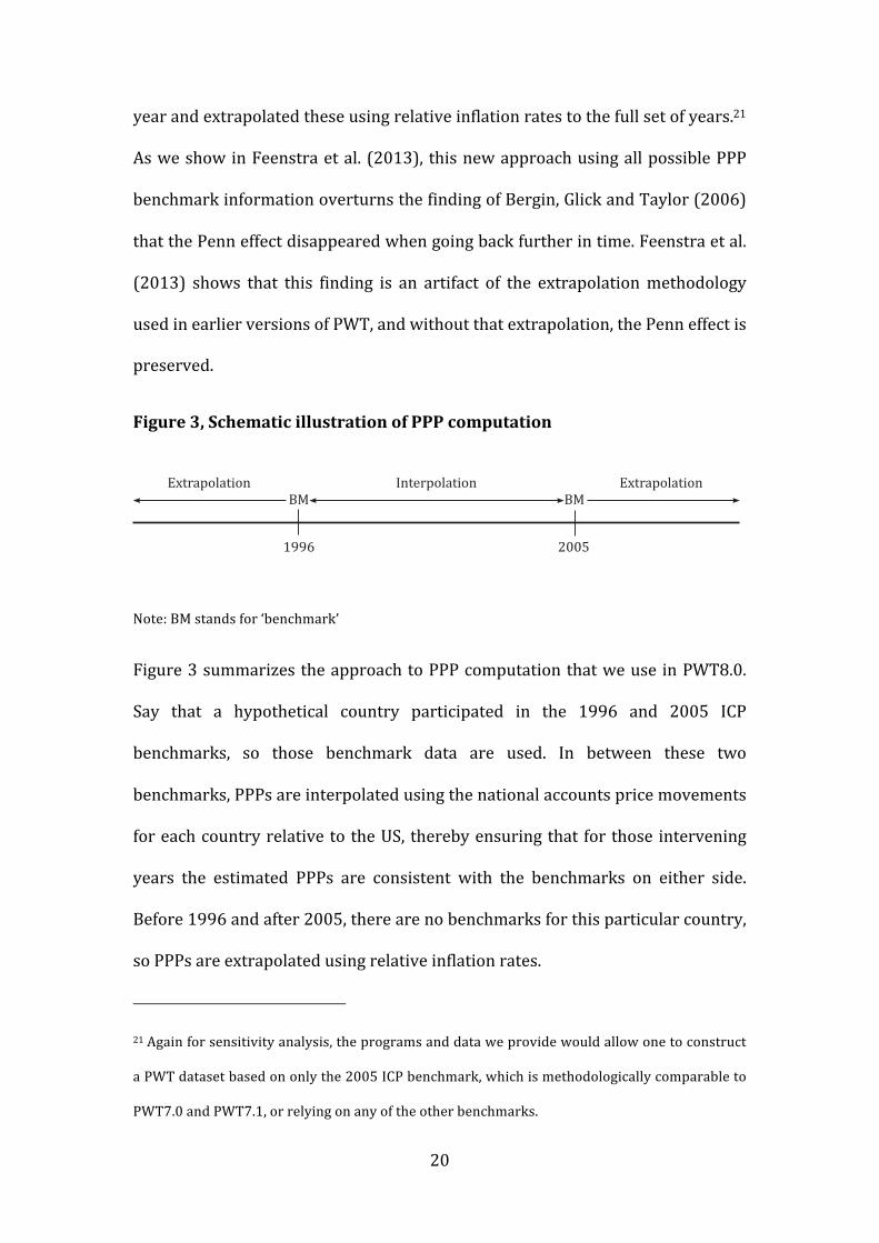
Figure  3,  Schematic  illustration  of  PPP  computation  

 

Note:  BM  stands  for  ‘benchmark’  

Figure  3  summarizes  the  approach  to  PPP  computation  that  we  use   in  PWT8.0.  

Say   that   a   hypothetical   country   participated   in   the   1996   and   2005   ICP  

benchmarks,   so   those   benchmark   data   are   used.   In   between   these   two  

benchmarks,  PPPs  are  interpolated  using  the  national  accounts  price  movements  

for  each  country  relative  to  the  US,   thereby  ensuring  that   for  those   intervening  

years   the   estimated   PPPs   are   consistent   with   the   benchmarks   on   either   side.  

Before  1996  and  after  2005,  there  are  no  benchmarks  for  this  particular  country,  

so  PPPs  are  extrapolated  using  relative  inflation  rates.  

                                                                                                               

21  Again  for  sensitivity  analysis,  the  programs  and  data  we  provide  would  allow  one  to  construct  

a  PWT  dataset  based  on  only  the  2005  ICP  benchmark,  which  is  methodologically  comparable  to  

PWT7.0  and  PWT7.1,  or  relying  on  any  of  the  other  benchmarks.  

1996 2005

BM BMInterpolation ExtrapolationExtrapolation

  21  

The   second   lesson   is   that   any   PPP   extrapolation   should   be   done   at   a   detailed  

level,  so  not  for  GDP  as  a  whole,  but  for  different  components  of  GDP.  A  guiding  

principle   should   be   that   if   expenditure   shares   and   relative   price   trends   differ  

considerably  across  countries  and  over  time,  the  relative  change  of  an  aggregate  

price  index  will  not  adequately  capture  the  change  in  PPPs.  This  is  in  accordance  

with   earlier   PWT   practice,   whereby   PPPs   for   household   consumption,  

investment   and   government   consumption   are   separately   extrapolated   using  

price   trends   for  each  of   these  components   from  the  National  Accounts.   In  each  

year,   the   PPPs   for   the   three   components   are   then  weighted   using   expenditure  

shares  for  all  countries  to  arrive  at  a  GDP  PPP.    

The   results   of   Feenstra   et   al.   (2013)   on   the   Penn   effect   indicate,   though,   that  

even   this   extrapolation   below   the   GDP   level   can   lead   to   qualitatively   different  

patterns  in  the  data  than  benchmark  or  interpolated  observations.  This  suggests  

that  an  even  more  detailed  breakdown  of  GDP  would  be  preferable,  but   this   is  

not  readily  feasible  given  available  National  Accounts  data.  We  therefore  indicate  

for   each   observation   whether   it   is   based   on   a   PPP   benchmark,   interpolated  

between  PPP  benchmarks  or  extrapolated  using  relative  inflation.  This  way,  the  

robustness   of   any   findings   to,   for   instance,   including   real   GDP   observations  

based   on   extrapolated   PPPs,   can   be   established.   In   addition,  we   compared   the  

extrapolated  PPPs   to   benchmark   and   interpolated  PPPs   and   to   predicted  PPPs  

based  on  Penn  effect  regressions.  This  led  us  a)  to  replace  some  market  exchange  

rates   by   estimated   rates   whenever   price   levels   spiked   due   to   misaligned  

exchange   rates   and   b)   to   label   some   observations   as   outliers   whenever   price  

levels  would  be   systematically  outside  a   range  we   consider  plausible  based  on  

  22  

observed   benchmark   and   interpolated   price   levels   and   predicted   price   levels  

from  Penn  effect  regressions.  These  choices  are  motived  and  discussed  in  detail  

in  the  documentation  on  the  PWT  website.  

Implications  

The  choice  to  use  the  historical  PPP  survey  data  has  implications  for  the  use  of  

PWT  in  research.  Until  now,  there  has  always  been  a  clear  connection  between  

growth  of  GDP  at  constant  national  prices  and  the  change  in  real  GDP  over  time.  

Starting   from   a   single   benchmark   year,   PPPs   in   earlier   years   were   estimated  

using   national   price   trends.   Since   those   price   trends   are   the   same   as   those  

underlying   growth   of   GDP   at   constant   national   prices,   the   only   differences   in  

growth  rates  were  due  to  differences  in  the  weights  of  consumption,  investment  

and   government   expenditures,   used   to   aggregate   these   components   with   the  

trade   balance   to   total   GDP.22  However,   the   use   of  multiple   PPP   benchmarks   in  

constructing  real  GDP  in  PWT8.0  means  that  changes  in  real  GDP  will  now  show  

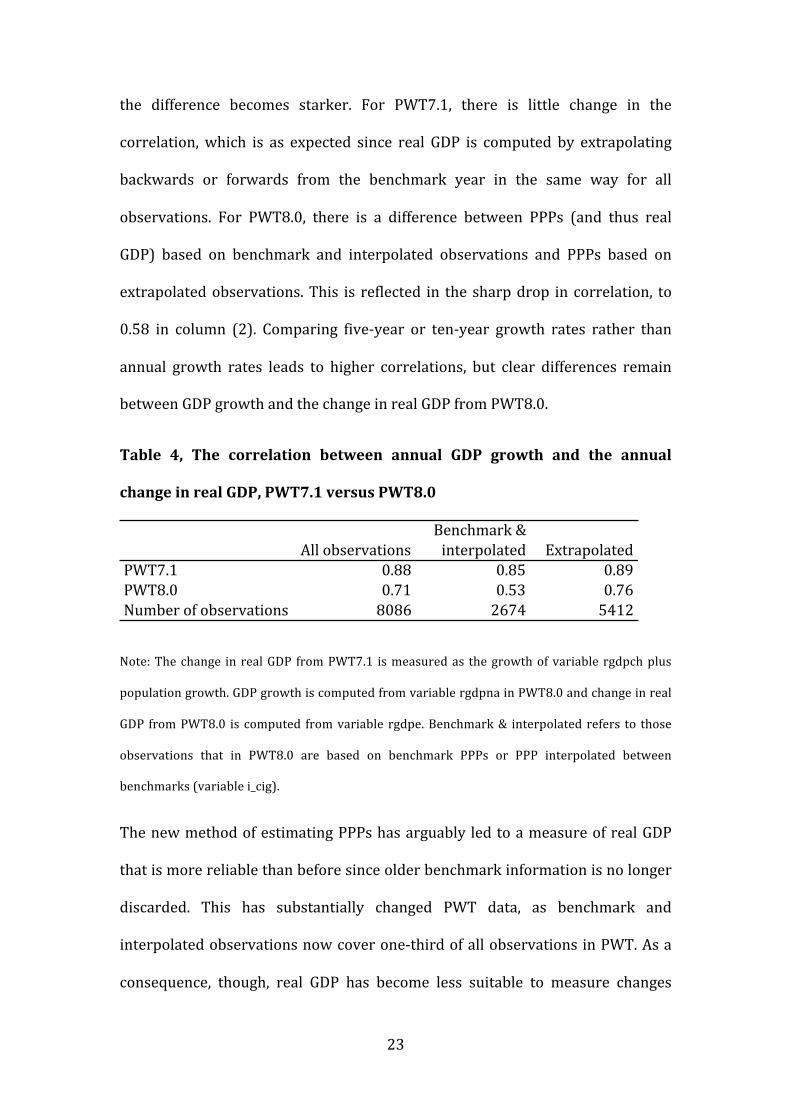
less  resemblance  to  growth  of  GDP  at  constant  national  prices.  This  is  confirmed  

in   Table   1,   which   shows   the   correlation   between   annual   GDP   growth   directly  

from  the  National  Accounts  and  the  change  in  real  GDP  from  PWT7.1  and  from  

PWT8.0.  Column  (1)  shows  that  both  real  GDP  measures  are  strongly  correlated  

with  GDP  growth  from  the  National  Accounts,  but  that  this  correlation  is  clearly  

higher  in  PWT7.1  than  in  PWT8.0.  Moreover,  when  splitting  the  sample  between  

observations  based  on  benchmark  or   interpolated  PPPs  and  extrapolated  PPPs,  

                                                                                                               

22  For   growth   of   GDP   at   constant   national   prices,   the  weights  would   be   expenditure   valued   at  

national  prices,  while  for  real  GDP  the  weights  would  be  expenditure  valued  at  reference  prices  

(i.e.  in  PPP-­‐converted  values).  

  23  

the   difference   becomes   starker.   For   PWT7.1,   there   is   little   change   in   the  

correlation,  which   is   as   expected   since   real   GDP   is   computed   by   extrapolating  

backwards   or   forwards   from   the   benchmark   year   in   the   same   way   for   all  

observations.   For   PWT8.0,   there   is   a   difference   between   PPPs   (and   thus   real  

GDP)   based   on   benchmark   and   interpolated   observations   and   PPPs   based   on  

extrapolated  observations.  This   is   reflected   in   the  sharp  drop   in   correlation,   to  

0.58   in   column   (2).   Comparing   five-­‐year   or   ten-­‐year   growth   rates   rather   than  

annual   growth   rates   leads   to   higher   correlations,   but   clear   differences   remain  

between  GDP  growth  and  the  change  in  real  GDP  from  PWT8.0.  

Table   4,   The   correlation   between   annual   GDP   growth   and   the   annual  

change  in  real  GDP,  PWT7.1  versus  PWT8.0  

 

Note:  The  change   in   real  GDP   from  PWT7.1   is  measured  as   the  growth  of  variable   rgdpch  plus  

population  growth.  GDP  growth  is  computed  from  variable  rgdpna  in  PWT8.0  and  change  in  real  

GDP   from  PWT8.0   is   computed   from  variable   rgdpe.  Benchmark  &   interpolated  refers   to   those  

observations   that   in   PWT8.0   are   based   on   benchmark   PPPs   or   PPP   interpolated   between  

benchmarks  (variable  i_cig).  

The  new  method  of  estimating  PPPs  has  arguably   led  to  a  measure  of  real  GDP  

that  is  more  reliable  than  before  since  older  benchmark  information  is  no  longer  

discarded.   This   has   substantially   changed   PWT   data,   as   benchmark   and  

interpolated  observations  now  cover  one-­‐third  of  all  observations  in  PWT.  As  a  

consequence,   though,   real   GDP   has   become   less   suitable   to   measure   changes  

All#observationsBenchmark#&#interpolated Extrapolated

PWT7.1 0.88 0.85 0.89PWT8.0 0.71 0.53 0.76Number#of#observations 8086 2674 5412

  24  

over  time  in  a  single  country.  Real  GDP  has  always  been  less  than  ideal  for  this  

purpose,   as   it   is   estimated   using   information   on   spending   patterns   across   all  

countries.  Since  a  country’s  spending  pattern  is  the  result  of  its  own  preferences  

and   relative   prices,   other   countries’   spending   patterns   are   irrelevant   when  

measuring   the   economic   performance   of   a   single   economy   over   time.   So   if   an  

analysis  aims  to  explain  cross-­‐country  differences  in  GDP  growth  rates,  we  would  

strongly  recommend  using  data  on  the  growth  of  GDP  at  constant  national  prices,  

directly  based  on  a  country’s  National  Accounts.  To  facilitate  such  research,  we  

have   included  a  measure  of   real  GDP   in  PWT8.0  whose  growth  rate  equals   the  

National  Accounts  measure  of  real  GDP  growth  (i.e.  at  constant  national  prices),  

and  whose  level  in  the  benchmark  year  2005  equals  real  GDP  on  the  output  side,  

as  discussed  next.  

International  trade  PPPs  

As  a  second  major  change,  PWT8.0  introduces  a  new  measure  of  real  GDP  to  the  

dataset.   The   traditional   measure   is   based   only   on   prices   of   consumption   and  

investment,  i.e.  domestic  final  expenditure,  while  the  new  measure  also  accounts  

for   differences   in   the   prices   of   exports   and   imports.   Put   differently,   the   new  

measure  of   real  GDP  accounts   for  differences   in   the   terms  of   trade.  A  real  GDP  

measure  that  ignores  terms  of  trade  differences  is  certainly  relevant,  as  it  can  be  

seen  as  a  measure  of  real  income:  for  consumers  it  does  not  matter  if  income  is  

high   because   export   prices   are   relatively   favorable   or   because   productivity   is  

high.   But   for   comparing   the   productive   capacity   of   economies,   we   do  want   to  

make   such   a   distinction   and   account   for   favorable   (or   unfavorable)   terms   of  

  25  

trade   in   comparing   GDP   across   countries.23  PWT8.0   therefore   includes   two  

distinct  real  GDP  measures,  one  from  the  expenditure  side,  GDPe,  and  one  from  

the   output   side,   GDPo.   This   is   in   addition   to   the   real   GDP   measure,   RGDPNA,  

discussed  just  above,  which  equals  GDPo  in  2005  but  whose  growth  rate  is  taken  

from  the  National  Accounts  of  each  country.  

Computing   GDPo   requires   developing   new   information   on   the   relative   price   of  

exports   and   of   imports   as   these   prices   are   not   part   of   the   World   Bank’s   ICP  

program.  Instead,  the  World  Bank  makes  the  simplifying  assumption  that  the  law  

of  one  price  holds  for  traded  products  so  that  the  exchange  rate  can  be  used  to  

express   the   trade   balance   in   real   terms.   Yet   there   is  much   evidence   that   is   at  

odds   with   this   assumption.   The   review   by   Burstein   and   Gopinath   (2013)  

concludes  that  even  in  the  long-­‐run,  exchange  rate  movements  do  not  fully  ‘pass  

through’  to  export  and  import  prices  and  that  imperfect  competition  and  pricing-­‐

to-­‐market  seem  to  play  an  important  role  in  explaining  these  patterns.  

Yet  quantifying  these  price  differences  has  been  a  challenging  undertaking.  The  

only  readily  available  data  from  which  price  differences  of  exports  and  imports  

can  be  inferred  is  data  on  the  value  and  quantity  of  traded  products.  Dividing  the  

value   by   the   quantity   gives   a   unit   value,   but   this   is   only   an   average   price   of   a  

potentially  very  heterogeneous  bundle  of  products.24  Recent  research  by  Hallak  

and  Schott  (2011)  and  Feenstra  and  Romalis  (2012)  has  estimated  how  much  of  

                                                                                                               

23  This  argument  is  made  more  formally  in  Feenstra  et  al.  (2009).  

24  For  example,  one  product   in  the  6-­‐digit  Harmonized  System  list   is   ‘Color  television  receivers’  

and   that   is   the  most   detailed   level   available   in   a   wide   cross-­‐country   setting.   On   Amazon.com,  

television  prices  vary  between  $100  and  $50  000.  

  26  

the  observed  differences   in  unit   values   is  due   to  differences   in  product  quality  

and  how  much  is  due  to  actual  price  differences.  After  netting  out  the  portion  of  

unit-­‐value  differences  across  countries  that  are  due  to  quality,  the  remainder  is  

the  “quality-­‐adjusted  price”  component.  These  remainders  are  aggregated  up  to  

obtain  the  export  and  import  PPP  for  each  country  and  year.  Because  the  law  of  

one  price  is  closer  to  holding  for  traded  goods  than  for  non-­‐traded  goods,  these  

export  and  import  PPPs  are  closer  to  the  nominal  exchange  rates  of  countries.  

The  resulting  trade  PPPs  can  then  be  used  alongside  the  domestic  PPPs  from  the  

ICP.   By   dividing   the   trade   PPPs   by   the   nominal   exchange   rate,   we   obtain   the  

“price   levels”   of   exports   and   imports   for   each   country.   A   country   will   have  

favorable   terms   of   trade   if   it   receives   a   relatively   high   price   for   its   exports  

(compared  with  prices  received  by  other  countries  exporting  the  same  product)  

and  pays  a  relatively  low  price  for  its  imports  (again,  compared  with  prices  paid  

by   other   countries   importing   the   same   product).   This   will   tend   to   make   real  

GDPe  higher  than  real  GDPo.  The  impact  on  real  GDP  will  not  only  depend  on  the  

terms  of  trade,  however,  but  also  on  the  domestic  prices  obtained  by  dividing  the  

domestic  PPPs  by  the  nominal  exchange  rate.25  If  domestic  prices  are  lower  than  

trade  prices,  as  would  be  typical  for  a  developing  countries,  and  the  country  has  

a  real  balance  of   trade  surplus,   then  real  GDPe  will   tend  to  be  higher   than  real  

GDPo.   So   in   addition   to   the   terms   of   trade,   the   comparison   of   trade   prices   to  

domestic  prices  also  determine  the  gap  between  real  GDPe  and  real  GDPo,  which  

has   a   straightforward   interpretation:   countries   with   a   real   GDPe   level   that  

                                                                                                               

25    See  footnote  2.  

  27  

exceeds   their   real   GDPo   level   can   consume   in   excess   of   their   economy’s  

productive  capacity  and  vice  versa.    

We  caution  that  the  gap  between  real  GDPe  and  real  GDPo  is  not  a  measure  of  the  

gains  from  trade  for  countries,  or  at  least,  not  the  gains  from  trade  as  compared  

to   autarky   (i.e.   no   trade).    We   have   not   built   anything   into   the   calculations   in  

PWT8.0   that   would   allow   the   gains   as   compared   to   autarky   to   be   estimated.  

Rather,  this  gap  reflect  the  ability  of  countries  to  trade  as  prices  that  better  than  

the   average   world   prices   (i.e.   higher   for   exports   or   lower   for   imports).   By  

construction,  then,  the  sum  over  countries  of  real  GDPe  and  real  GDPo  should  be  

close  to  zero,  as  occurs  in  the  dataset  for  all  years.    

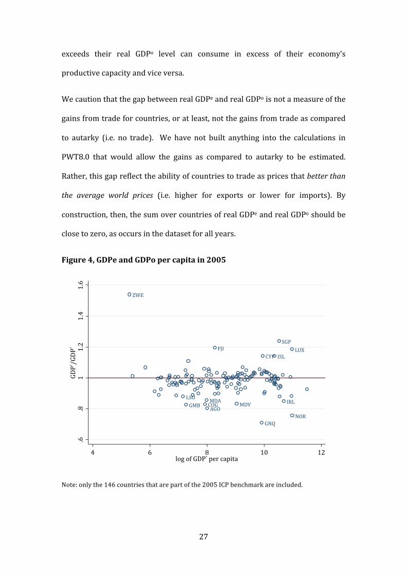
Figure  4,  GDPe  and  GDPo  per  capita  in  2005  

 

Note:  only  the  146  countries  that  are  part  of  the  2005  ICP  benchmark  are  included.  

AGOCOG

CYP

FJI

GMB

GNQ

IRL

ISL

LSO

LUX

MDAMDV

NOR

SGP

ZWE

.6.8

11.2

1.4

1.6

GDP>/GDP@

4 6 8 10 12logEofEGDP@EperEcapita

  28  

For   individual   countries,   the  gap  between  GDPe   and  GDPo   can  be   considerable.  

The  median  absolute  difference  is  3.2  percent  and  in  5  percent  of  the  countries,  

the   difference   is   even   larger   than   20   percent.   Figure   4   shows   the   difference  

between  GDPe  and  GDPo  per  capita  in  2005  set  against  log  of  GDPo  per  capita  in  

2005.  The  larger  differences  are  typically  observed  in  smaller,  open  economies.  

So  the  choice  between  GDPe  and  GDPo  clearly  matters.  

For  many   analyses,   it   is   now  possible   to  use   the   conceptually   appropriate   real  

GDP   measure.   For   instance,   for   analyzing   productivity   differences   across  

countries   (e.g.   Hall   and   Jones,   1999;   Caselli,   2005),   real   GDPo   would   be   the  

appropriate   measure,   while   for   comparing   cross-­‐country   wellbeing   (e.g.   Jones  

and  Klenow  2011),   real  GDPe  would  be  better   suited.   In   comparisons  of   cross-­‐

country  wellbeing,   the   effect   from   favorable  or  unfavorable   terms  of   trade   can  

and  should  now  also  be  taken  into  account.  

Moreover,   to   emphasize   the   breadth   of   new   information,  we   provide   not   only  

provides   PPPs   for   total   exports   and   imports,   but   also   distinguished   by   “broad  

economic  categories”  (BEC).  This  breakdown  by  BEC  means  that  a  distinction  is  

made  of  the  prices  paid  for,  for  example,  imports  of  capital  goods  versus  imports  

of   industrial   materials.   This   could,   for   instance,   shed   new   light   on   the   role   of  

imported  technology,  as  highlighted  in  Caselli  and  Wilson  (2004),  by  accounting  

for  price  differences  of  imported  capital  goods.  

Implications  

The   newly   developed   international   trade   prices   increase   the   number   of   GDP  

concepts   that   are   included   in  PWT8.0.   In   addition,  we  distinguish  between   the  

traditional  real  GDP  measures  and  current-­‐price  measures.  Table  5  summarizes  

  29  

the  resulting  five  measures.  The  first,  RGDPNA  is  primarily  suited  for  measuring  

economic  growth  of  a  particular  country  over  time.  Its  level  in  2005  is  the  same  

as  RGDPo  and  CGDPo,  but  its  growth  rate  is  equal  to  that  in  the  National  Accounts.  

The  next   two,  CGDPe  and  CGDPo,  give  the  best  estimate  of   the   level  of  GDP  in  a  

country  relative  to  another  at  a  single  point  in  time,  where  CGDPe  is  a  measure  of  

comparative  living  standards  and  CGDPo  is  a  measure  of  comparative  productive  

capacity.   To   make   the   magnitudes   comparable   over   time,   we   account   for   US  

inflation,  but  changes  in  CGDP  levels  should  not  be  seen  as  measure  of  economic  

growth.  Finally,  there  are  two  real  GDP  measures,  RGDPe  and  RGDPo.  These  aim  

to   comparable   across   countries   and   over   time,   see   Feenstra   et   al.   (2013)   for  

details.  These  measures  are  primarily  useful   to  compare   trends   in  comparative  

living  standards  (RGDPe)  or  in  productive  capacity  (RGDPo).  This  can  give  insight  

on  such  questions  as  how  rich  is  China  compared  with  the  US  in  1950.  In  2005,  

RGDPo  equals  CGDPo  and  RGDPe  equals  CGDPe.  

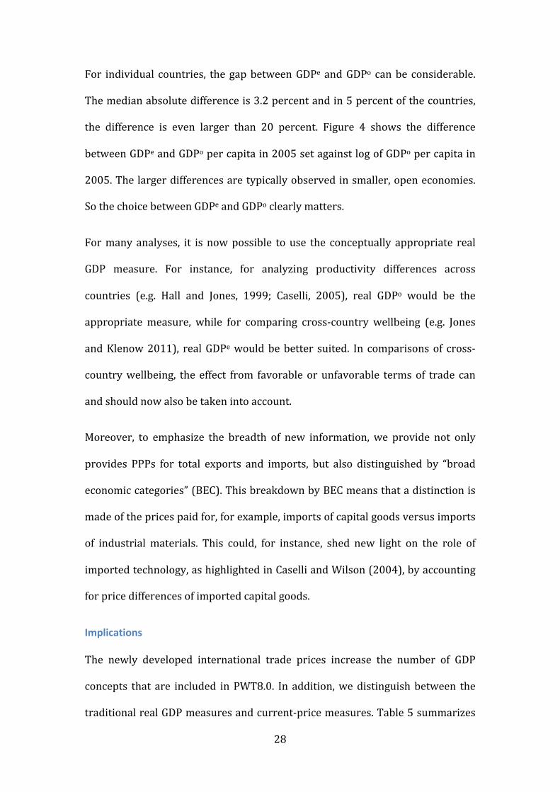
Table  5,  GDP  concepts  in  PWT8.0  and  their  use  

Series   Best  use   Example  

RGDPNA  

 

Studies  only  requiring  (output-­‐based)  growth  rates  over  time  and  comparing  growth  rates  across  countries  

Dependent  variable  in  (cross-­‐country)  growth  regressions  

CGDPe   Expenditure-­‐based,  to  compare  relative  living  standards  across  countries  at  a  single  point  in  time  

Initial  level  in  growth  regressions  requiring  relative  living  standards  

CGDPo   Output-­‐based,  to  compare  relative  productivity  capacity  across  countries  at  a  single  point  in  time  

Initial  level  in  growth  regressions  requiring  productive  capacity  or  productivity  

RGDPe   Expenditure-­‐based,  to  compare  relative  living  standards  across  

Living  standards  of  China  today  compared  to  the  US  at  some  point  

  30  

countries  and  over  time   in  the  past  

RGDPo   Output-­‐based,  to  compare  relative  productivity  capacity  across  countries  and  over  time  

Productive  capacity  of  China  today  compared  to  the  US  at  some  point  in  the  past  

Capital  and  productivity  

The  construction  of  the  data  on  capital  and  productivity  in  PWT8.0  are  discussed  

in  detail  in  Inklaar  and  Timmer  (2013c),  but  it  is  helpful  to  highlight  some  of  the  

main   features   and   limitations.   In   the   past,   PWT   data   has   often   been   used   to  

construct  measures  of  total  factor  productivity  (TFP),  such  as  by  Hall  and  Jones  

(1999)   and   Caselli   (2005).   These   would   typically   use   GDP   per   worker   as   the  

measure  of  labor  productivity  and  correct  for  differences  in  tangible  capital  per  

worker   and   human   capital   per   worker,   as   in   Table   1.   PWT8.0   improves   upon  

those  earlier  approaches  in  two  important  ways:  

1. Rather   than   assuming   a   single   depreciation   rate   that   is   constant   across  

countries   and   over   time,   we   allow   this   to   be   different.   By   distinguishing  

investment  in  up  to  six  types  of  assets,  including  at  least  machinery,  transport  

equipment   and   buildings,   our   depreciation   rate   will   vary   across   countries  

and  over  time.  

2. Rather  than  assuming  a  single  share  of  labor  compensation  in  GDP  to  weight  

the   importance  of  human  versus  physical   capital,  we  have  constructed  new  

measures  from  basic  National  Accounts  data.  

These   improvements,   and   in   particular   the   use   of   a   country-­‐specific   and   year-­‐

specific   labor   share,   help   to   reduce   the   role   of   TFP   differences   in   explaining  

cross-­‐country  income  differences,  as  we  show  in  Feenstra  et  al.  (2013).  Similar  to  

  31  

the  distinction  between  different  GDP  measures   in  Table  5,   PWT8.0   includes   a  

TFP   measure   that   allows   for   comparisons   across   countries   at   a   point   in   time  

(variable  CTFP)  and  a  measure  that  allows  comparisons  within  countries  across  

the  years  (RTFPNA).  Despite  the  improvements  over  earlier  work,  there  are  still  

shortcomings  in    the  TFP  measures  in  PWT8.0  due  to  a  lack  of  data:  

1. Capital  services.  Jorgenson  and  Griliches  (1967)  argued  that  not  every  dollar’s  

worth   of   capital   generates   the   same   return.   Shorter-­‐lived   assets,   such   as  

computers  would  be  expected  to  earn  a  greater  productive  return  than  long-­‐

lived  assets,  such  as  buildings.  Practical  difficulties  in  determining  a  required  

rate   of   return   across   countries   and   over   time   have   stopped   us   from  

implementing  such  an  approach.  This  is  likely  to  underestimate  capital  input  

mostly   in   the   richer   economies   where   investment   in   information   and  

communication  technologies  is  highest.26  

2. Land,  inventories,  subsoil  assets  and  intangibles.  Our  current  set  of  assets  only  

covers   the   so-­‐called   fixed   reproducible   assets   recognized   in   the   System   of  

National  Accounts.  Differences  in  the  availability  of  land,  inventories,  subsoil  

assets  (e.g.  World  Bank,  2006)  or  intangible  assets  (e.g.  Corrado,  Hulten  and  

Sichel,  2009)  are  not  taken  into  account.  This  will  understate  capital  input  in  

oil-­‐producing  and  other  resource-­‐intensive  countries;  in  countries  with  large  

arable   land   areas;   and   in   richer   economies   that   increasingly   rely   on  

investment  in  intangible  assets.  

                                                                                                               

26  The   Total   Economy   Database   of   The   Conference   Board   does   provide   TFP   growth  measures  

based  on  growth  in  capital  services  rather  than  growth  in  the  capital  stock  as  in  PWT.  

  32  

3. Hours  worked.  Data  on  the  number  of  persons  engaged  could  be  constructed  

for   164   out   of   167   countries   in   PWT,   but   data   on   average   annual   hours  

worked  is  only  available  for  52  countries  (from  the  Total  Economy  Database  

of  The  Conference  Board).  Hours  worked  vary  between  1380  and  2800  hours  

per  year,  with  richer  countries  working  relatively  fewer  hours.  Labor  input  of  

the  poorer  countries  is  thus  underestimated  by  using  the  number  of  workers.  

4. Human  capital.  To  account   for  differences   in  human  capital,  we  use  data  on  

the  average  years  of   schooling   from  Barro  and  Lee   (2010)  and  use   rates  of  

return   for   completing   different   sets   of   years   of   education   (Psacharopoulos,  

1994).   This   ignores   any   variation   in   these   returns   over   time   or   across  

countries.  Likewise,  it  ignores  differences  in  the  cognitive  skills  that  students  

obtain,  which  may  be  more  important  than  the  simply  the  number  of  years  in  

school   (Hanushek   and   Woessman,   2012).   Ignoring   cognitive   skills   likely  

underestimates   labor   input   in   richer   countries   as   richer   countries   have  

higher  cognitive  skills  given  the  average  years  of  schooling.  However,  data  do  

not  allow  a  cognitive  skills  measure   to  be   implemented   for  a  broad  enough  

sample  that  also  includes  variation  over  time.  

Despite   these   shortcomings,  we  believe   the   current  data  on   relative  TFP   levels  

and  on  TFP  growth  in  PWT8.0  represent  a  useful  improvement  over  earlier  work  

and   the   list   of   shortcomings   is   an   open   invitation   to   realize   further  

improvements.  

National  Accounts  

Besides  the  PPP  benchmark  data,  the  other  main  data  input  of  PWT  is  National  

Accounts   (NA)   data.   These   data   are   used,   first,   to   estimate   PPPs   where  

  33  

benchmark   or   interpolated   data   is   not   available   using   national   price   indices.27  

Second,  PWT  relies  on  NA  for  data  on  GDP  at  national  prices,  which  is  converted  

to   real   GDP  using   the  GDPe   and  GDPo   PPPs.   Comparative  GDP   figures   are   thus  

subject  to  change  if  the  underlying  NA  data  are  revised.  In  advanced  economies,  

such   revisions   are   typically   quantitatively   small.   For   example,   the   2009  

Comprehensive  Revision  by  the  US  Bureau  of  Economic  Analysis  revised  US  GDP  

in  2008  upwards  by  1.2  percent   (Seskin  and  Smith,  2009),  neither  a  negligible  

nor  a  substantial  change.  Changes  of  similar  magnitude  are   likely   to  be  seen   in  

more   countries,   for   instance   as   the   accounting   rules   of   the   System  of  National  

Accounts  (SNA)  1993  are  replaced  by  those  of  SNA  2008.    

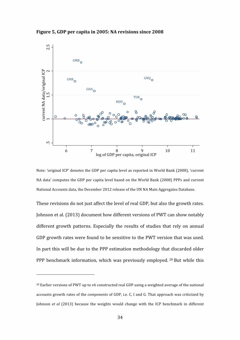
In  contrast,  Ghana  revised  its  GDP  upwards  by  60  percent  in  2010  (Jerven,  2013).  

Although  such  a  large  revision  is  not  typical,  it  is  also  not  as  unusual  as  may  be  

hoped.   Figure   5   compares   GDP   per   capita   in   2005   as   published   originally   in  

World  Bank  (2008)  with  GDP  per  capita  using  the  most  recent  NA  data.  It  shows  

that   Gambia’s   GDP   per   capita   has  more   than   doubled   after   revisions   in   recent  

years   and   even   Turkey’s   GDP   per   capita   has   increased   by   over   40   percent.   In  

contrast,  the  median  absolute  revision  is  a  more  modest  3.4  percent.  As  in  Figure  

4,   the   broad   cross-­‐country   pattern   is   not   materially   affected.   The   correlation  

between  the  two  sets  of  GDP  per  capita  numbers  in  Figure  5  is  0.996,  though  that  

is  scant  comfort  if  your  main  interest  is  the  level  of  living  standards  in  Ghana.  

                                                                                                               

27  For   interpolation   between   benchmarks,   we   also   use   national   accounts   price   indexes   to  

determine   the   precise   year-­‐to-­‐year   pattern   instead   of   doing   a   linear   interpolation.   This   is   a  

second-­‐order  impact  of  these  data.  

  34  

Figure  5,  GDP  per  capita  in  2005:  NA  revisions  since  2008  

 

Note:  ‘original  ICP’  denotes  the  GDP  per  capita  level  as  reported  in  World  Bank  (2008),  ‘current  

NA  data’  computes  the  GDP  per  capita   level  based  on  the  World  Bank  (2008)  PPPs  and  current  

National  Accounts  data,  the  December  2012  release  of  the  UN  NA  Main  Aggregates  Database.  

These  revisions  do  not  just  affect  the  level  of  real  GDP,  but  also  the  growth  rates.  

Johnson  et  al.  (2013)  document  how  different  versions  of  PWT  can  show  notably  

different   growth   patterns.   Especially   the   results   of   studies   that   rely   on   annual  

GDP  growth  rates  were  found  to  be  sensitive  to  the  PWT  version  that  was  used.  

In  part  this  will  be  due  to  the  PPP  estimation  methodology  that  discarded  older  

PPP  benchmark   information,  which  was  previously   employed.  28  But  while   this  

                                                                                                               

28  Earlier  versions  of  PWT  up  to  v6  constructed  real  GDP  using  a  weighted  average  of  the  national  

accounts  growth  rates  of  the  components  of  GDP,  i.e.  C,  I  and  G.  That  approach  was  criticized  by  

Johnson   et   al   (2013)   because   the   weights   would   change   with   the   ICP   benchmark   in   different  

GNQ

GMB

GHA

GNB

MDVTUR

.51

1.5

22.5

current7NA7data/original7ICP

6 7 8 9 10 11log7of7GDP7per7capita,7original7ICP

  35  

source   of   variation   across   PWT   version   will   be   much   reduced   by   our   newly  

adopted   methodology,   NA   revisions   are   another   source   of   variation.   Table   6  

illustrates  this  for  two  UN  NA  ‘vintages’,  the  first  with  data  up  to  2009  (released  

December  2010)  and  the  second  with  data  up  to  2011  (released  December  2012).  

The   table   compares   two   sets   of   growth   rates,   one   for   2009   and   one   for   1995;  

2009  is  the  latest  year  that  can  be  compared,  while  1995  is  chosen  as  an  earlier  

year   for   which   revisions   are   (presumably)   no   longer   as   substantial.   For   both  

years,  we  compare  the  annual  growth  rate,  the  five-­‐year  average  annual  growth  

rate   and   the   ten-­‐year   average   annual   growth   rate,   following   the   findings   by  

Johnson  et  al.  (2013)  that  average  growth  over  these  longer  time  spans  is  more  

stable   across  PWT  versions.  The   table   shows   the  5th   and  95th   percentile   of   the  

revision   to   growth   rates   across   the   two   vintages   as   well   as   the   correlation  

between  the  growth  rates  in  the  two  vintages.    

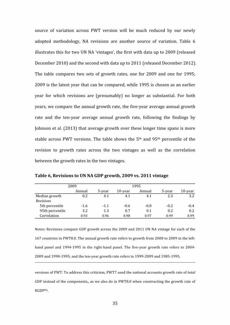
Table  6,  Revisions  to  UN  NA  GDP  growth,  2009  vs.  2011  vintage  

 

Notes:  Revisions  compare  GDP  growth  across  the  2009  and  2011  UN  NA  vintage  for  each  of  the  

167  countries  in  PWT8.0.  The  annual  growth  rate  refers  to  growth  from  2008  to  2009  in  the  left-­‐

hand   panel   and   1994-­‐1995   in   the   right-­‐hand   panel.   The   five-­‐year   growth   rate   refers   to   2004-­‐

2009  and  1990-­‐1995;  and  the  ten-­‐year  growth  rate  refers  to  1999-­‐2009  and  1985-­‐1995.                                                                                                                                                                                                                                                                                                                                

versions  of  PWT.  To  address  this  criticism,  PWT7  used  the  national  accounts  growth  rate  of  total  

GDP  instead  of  the  components,,  as  we  also  do  in  PWT8.0  when  constructing  the  growth  rate  of  

RGDPNA.    

2009 1995Annual 5+year 10+year Annual 5+year 10+year

Median2growth 0.2 4.1 4.1 4.1 2.3 3.2Revisions5th2percentile +1.6 +1.1 +0.6 +0.8 +0.2 +0.495th2percentile 3.2 1.3 0.7 0.1 0.2 0.2Correlation 0.93 0.96 0.98 0.97 0.99 0.99

  36  

The   results   in   Table   6   confirm   the   Johnson   et   al.   (2013)   finding   that   long-­‐run  

growth  rates  are   less  affected  by  NA  revisions   than  annual  growth  rates  as   the  

90-­‐percent   range  of   revisions   shrinks   considerable,   from  4.8   to  1.3  percentage  

points   for  growth  rates  up  to  2009  and  from  0.9  to  0.6  percentages   for  growth  

rates   up   to   1995.   This   also   confirms   that  more   recent   data   are  more   likely   to  

change   due   to   NA   revisions.   This   is   unsurprising,   as   the  most   up-­‐to-­‐date   GDP  

growth  numbers  tend  to  be  based  on  incomplete  source  data.  The  cross-­‐country  

correlations  at  the  bottom  of  the  table  indicate  that  rapidly-­‐growing  countries  in  

one  vintage  also  tend  to  grow  fast  in  the  other  vintage,  but  a  correlation  of  0.93  

for  annual  growth  in  2009  indicates  notable  variation.  

To  help  assess  the  sensitivity  of  any  research  results  to  the  NA  vintage  used,  we  

provide   the   2009   and   2010   NA   data   vintages.29  In   addition,   we   include   the  

statistical   capacity   indicator   of   the   World   Bank   in   PWT8.0.   This   indicator   is  

constructed  since  1999  for  developing  economies  and  it   is  based  on  the  quality  

of  the  statistical  methodology,  frequency  with  which  source  data  is  collected  and  

the   timeliness   with   which   data   is   provided.   Not   all   of   these   aspects   refer  

(directly)  to  NA  data,  but  this  indicator  can  be  useful  to  assess  the  reliability  of  a  

country’s  data.30  

China  

China  also  deserves  some  attention  in  regards  to  its  NA.  As  discussed  above,  the  

2005   ICP   results   underestimated   China’s   GDP   level,   which   we   adjust   for   in                                                                                                                  

29  Old  vintages  are  not  made  available  by  the  UN.  

30  The  work  by   Jerven  (2013),  Devarajan  (2013)  and  Young  (2012)  are  useful   in   this   regard  as  

well.  

  37  

PWT8.0  as  in  PWT7.0  and  7.1.  In  addition,  there  have  long  been  doubts  about  the  

accuracy   of   China’s   growth   figures.   In   the   academic   literature,   the   debate   has  

been  between  those  arguing  that  the  official  statistics  get  it  broadly  right  (Holz,  

2006)  and  others  arguing  that  official  statistics  systematically  overstate  growth  

(Maddison   2006;   Maddison   and   Wu,   2008).   We   find   the   ‘overstatement’  

argument  convincing  and  use  alternative  NA  data  based  on  data  from  Wu  (2011).  

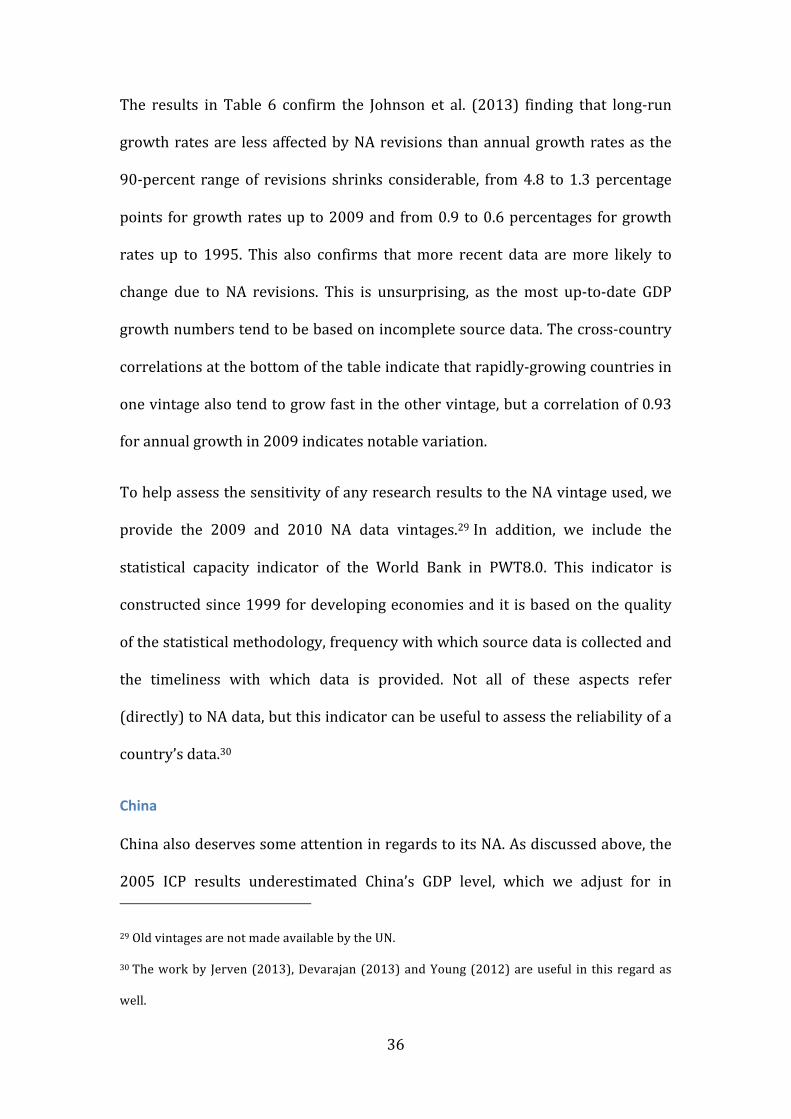
Table   7   shows   average   annual   GDP   growth   for   each   decade   since   1952,  

comparing   the   official  NA   data   to   the   adjusted  GDP   data  we   use   in   PWT8.0.   It  

show   that   the   degree   to   which   growth   is   overstated   varies   considerably   over  

time,  but   is  present   in  every  period.  As  a  result,   the  GDP   level   in  1952   is  more  

than  twice  as  high  according  to  the  adjusted  growth  figures  than  according  to  the  

official  growth  figures.  Since  China  participated  in  an  ICP  comparison  for  the  first  

time   only   in   2005,   there   is   no   readily   available   independent   information   for   a  

possible  cross-­‐check  of  this  result.  While  we  present  data  based  on  the  adjusted  

2005   PPP   and   adjusted   growth   rates   in   PWT8.0,   we   also   provide   the   data   to  

construct  an  alternative  dataset  using  official  PPPs  and  growth  rates  for  China.  

Table  7,  Average  annual  GDP  growth  in  China  1952-­‐2010,  adjusted  versus  

official  

 

Note:  adjusted  GDP  growth  is  provided  by  Harry  Wu,  based  on  Wu  (2011);  official  data  is   from  

the  UN  NA  (December  2012  version).  The  adjusted  growth  series  are  used  in  PWT8.0.  

Official Adjusted Difference195251960 6.2 5.4 0.8196051970 3.3 2.8 0.5197051980 6.2 4.6 1.6198051990 9.3 6.2 3.0199052000 10.4 7.1 3.3200052010 10.5 9.2 1.3

  38  

Concluding  remarks  

In   this   guide,   we   have   explained   and   motivated   the   choices   we   made   in  

constructing   PWT8.0   and   discussed   the   implications   of   these   choices   for  

researchers  using  PWT.  To  summarize,  we  recommend  the  following:  

1. Use   GDPe   and   GDPo   series   only   as   a   measure   of   the   relative   level   across  

countries.   For   comparing   GDP   growth,   use   the   series   of   GDP   at   constant  

national  prices  from  the  National  Accounts  data,  RGDPNA.  

2. Use   GDPe   when   interested   in   comparative   well-­‐being;   use   GDPo   when  

interested  in  an  economy’s  productive  capacity.  

3. Beware  that  observations  in  PWT  that  are  directly  based  on  PPP  benchmark  

data   or   interpolations   between   PPP   benchmarks   are   more   reliable   than  

observations   based   on   extrapolations   from   benchmarks   and   can   show  

differences  in  patterns  such  as  the  Penn  effect.  

4. Beware   that   there   is   a   greater   margin   of   uncertainty   when   comparing  

countries  with  very  different  spending  patterns.  

5. Beware   that   revisions   to   National   Accounts   data   can   have   a   substantial  

impact  on  the  level  of  GDP  and  on  GDP  growth  rates  and  that  such  revisions  

are  typically  the  dominant  reason  for  changing  data  between  PWT  versions.  

Not   all   recommendations   will   be   equally   relevant   to   all   types   of   users.   For  

instance,  recommendation  4  would  mostly  be  relevant  when  comparing  a  single  

country’s  GDPe  or  GDPo  per   capita  or  PPP   to  other   countries.   Furthermore,  we  

provide   the   basic   data   and   programs   so   that   alternative   PWT   datasets   can   be  

constructed,  for  instance  based  on  a  different  index  number  method  or  on  official  

rather  than  adjusted  Chinese  data.  

  39  

This  guide  was  explicitly  aimed  at  a  non-­‐technical  audience,   the  Feenstra  et  al.  

(2013)   paper   discusses   the  more   technical   aspects   and   the  main   new   insights  

from   PWT8.0,   while   Inklaar   and   Timmer   (2013c)   discuss   the   new   capital   and  

TFP   data   in   more   detail.   This   guide   could   also   not   discuss   some   of   the   more  

detailed   aspects   of   PWT.   To   cover   those   aspects,   there   is   additional  

documentation  available  on:  

• The   technical   details   on   how   the   different   data   sources   are   combined   and  

how  PWT  is  constructed  in  Stata  [Technical  guide  to  PWT8.0],  

• The   differences   in   methodology,   results   and   variable   naming   between  

PWT7.1  and  PWT8.0  [Comparing  PWT8.0  with  7.1],  

• How   data   on   capital   and   TFP   have   been   constructed   [Capital   and   TFP   in  

PWT8.0],  

• The   sources  of  NA  data,   variable  definitions   and  accounting   rules   [National  

Accounts  in  PWT8.0],  

• The  choice  for  a  particular  exchange  rate  series  [Exchange  rates  in  PWT8.0],  

• The  identification  of  outliers  [Outliers  in  PWT8.0].  

While   the   appeal   of   a   dataset   with   information   on   economic   performance   for  

most  countries  in  the  world  over  the  past  60+  years  is  obvious,  it  is  of  little  use  if  

used  without  due  regard  of  the  choices  and  limitations  that  underlie  it.  We  hope  

that  this  guide  has  given  a  better  understanding  of  the  PWT8.0  dataset,  so  that  it  

is  used  to  its  greatest  potential.  

  40  

References  

Aghion,   Phillipe   and   Peter   Howitt   (2006),   “Appropriate   Growth   Policy:   A  Unifying  Framework”  Journal  of  the  European  Economic  Association  4(2-­‐3):  269-­‐314.  

Almås,  Ingvild  (2012),  “International  Income  Inequality:  Measuring  PPP  Bias  by  Estimating   Engel   Curves   for   Food”   American   Economic   Review   102(1):  1093-­‐1117.  

Ashraf,  Quamrul  and  Oded  Galor  (2012),  “The  “Out  of  Africa”  Hypothesis,  Human  Genetic   Diversity,   and   Comparative   Economic   Development”   American  Economic  Review  103(1):  1-­‐46.  

Balk,   Bert   M.   (2008),   Price   and   Quantity   Index  Numbers:  Models   for  Measuring  Aggregate  Change  and  Difference,  Cambridge  University  Press,  Cambridge.  

Barro,   Robert   J.,   and   Jong-­‐Wha   Lee   (2010),   “A   new   data   set   of   educational  attainment  in  the  world,  1950-­‐2010”  NBER  Working  Paper  no  15902.  

Bergin,   Paul   R.,   Reuven   Glick   and   Alan   M.   Taylor   (2006),   “Productivity,  tradability   and   the   long-­‐run   price   puzzle”   Journal   of  Monetary  Economics  53:  2041-­‐2066.  

Burstein,   Ariel   and   Gita   Gopinath   (2013),   "International   Prices   and   Exchange  Rates,"  prepared  for  the  Handbook  of  International  Economics,  vol.  IV.  

Caselli,  Francesco  (2005),  “Accounting  for  Cross-­‐Country  Income  Differences”  in  Philippe   Aghion   and   Steven   N.   Durlauf   (eds.)   Handbook   of   Economic  Growth,  volume  1A,  Elsevier,  Amsterdam,  679-­‐741.  

Caselli,  Francesco  and  Daniel  J.  Wilson  (2004),  “Importing  technology”  Journal  of  Monetary  Economics  51:  1-­‐32.  

Corrado,  Carol,  Charles  Hulten  and  Daniel  Sichel  (2009),  “Intangible  capital  and  U.S.  economic  growth”  Review  of  Income  and  Wealth  55(3):  661-­‐685.  

Davarajan,   Shantayanan   (2013),   “Africa’s   Statistical   Tragedy”  Review  of   Income  and  Wealth,  forthcoming.  

Deaton,   Angus   (2012),   “Consumer   price   indexes,   purchasing   power   parity  exchange   rates,   and   updating”   paper   presented   at   the   Penn  World   Table  Workshop,  May  2012.  

Deaton,   Angus   and   Alan   Heston   (2010),   “Understanding   PPPs   and   PPP-­‐based  National  Accounts”  American  Economic  Journal:  Macroeconomics  2(4):  1-­‐35.  

Diewert  W.   Erwin   (2002),   “Similarity   and   Dissimilarity   Indexes:   An   Axiomatic  Approach”  UBC  Discussion  Paper,  no.  02-­‐10.  

Diewert   W.   Erwin   (2013),   “Methods   of   Aggregation   above   the   Basic   Heading  Level  within   Regions”   in  World   Bank   (ed.)  Measuring   the  Real  Size  of   the  World  Economy,  World  Bank:  Washington  DC,  Chapter  5.  

Feenstra,   Robert   C.   and   John   Romalis   (2012),   “International   Prices   and  Endogenous  Quality”  NBER  Working  Paper,  no.  18314.  

Feenstra,   Robert   C.,   Alan   Heston,   Marcel   P.   Timmer,   and   Hayan   Deng   (2009)  “Estimating  Real  Production  and  Expenditures  Across  Nations:  A  Proposal  for   Improving   the  Penn  World  Tables”  Review  of  Economics  and  Statistics,  91(1),  201–12.  

Feenstra,  Robert  C.,  Hong  Ma,  J.  Peter  Neary  and  D.S.  Prasada  Rao  (2013),  “Who  Shrunk  China?  Puzzles  in  the  Measurement  of  Real  GDP”  Economic  Journal,  forthcoming.  

Feenstra,  Robert  C.,  Robert  Inklaar  and  Marcel  Timmer  (2013),  “PWT:  The  Next  

  41  

Generation,”   University   of   California,   Davis   and   University   of   Groningen,  draft,  2012.  

Hall,  Robert  E.  and  Charles  I.  Jones  (1999),  “Why  do  some  countries  produce  so  much  more  output  per  worker  than  others?”  Quarterly  Journal  of  Economics  114(1):  83-­‐116.  

Hallak,   Juan   Carlos   and   Peter   K.   Schott   (2011)   “Estimating   Cross-­‐Country  Differences   in   Product   Quality”   Quarterly   Journal   of   Economics,   126(1),  417–74.  

Hanushek,   Eric   A.   and   Ludger  Woessmann   (2012),   “Do   better   schools   lead   to  more  growth?  Cognitive  skills,  economic  outcomes,  and  causation”  Journal  of  Economic  Growth  17(4):  267-­‐321.  

Heston,  Alan  (2013)  “Government  Services:  Productivity  Adjustments”  in  World  Bank   (ed.)   Measuring   the   Real   Size   of   the   World   Economy,   World   Bank:  Washington  DC,  Chapter  16.  

Holz,  Carsten  A.  (2006),  “China’s  Reform  Period  Economic  Growth:  How  Reliable  Are  Angus  Maddison’s  Estimates?”  Review  of  Income  and  Wealth  52(1):  85-­‐119.  

Inklaar,  Robert  and  Marcel  P.  Timmer  (2013a),   “The  Relative  Price  of  Services”  Review  of  Income  and  Wealth,  forthcoming.  

Inklaar,  Robert  and  Marcel  P.  Timmer  (2013b),  “A  Note  on  Extrapolating  PPPs”  in  World  Bank   (ed.)  Measuring  the  Real  Size  of  the  World  Economy,  World  Bank:  Washington  DC,  Chapter  18,  Annex  D.  

Inklaar,   Robert   and   Marcel   P.   Timmer   (2013c),   “Capital   and   TFP   in   PWT8.0”  mimeo,  see  www.ggdc.net/pwt.  

Jerven,  Morten   (2013),   “Comparability  of  GDP  estimates   in  Sub-­‐Saharan  Africa:  the  effect  of  revisions  in  sources  and  methods  since  structural  adjustment”  Review  of  Income  and  Wealth,  forthcoming.  

Johnson,   Simon,  William   Larson,   Chris   Papageorgiou   and   Arvind   Subramanian  (2013),  “Is  newer  better?  Penn  World  Table  Revisions  and  their  impact  on  growth  estimates”  Journal  of  Monetary  Economics,  forthcoming.  

Jones,   Charles   I.   and   Peter   J.   Klenow   (2011),   “Beyond   GDP?   Welfare   across  Countries  and  Time”  NBER  Working  Paper,  no.  16352.  

Kravis,  Irving  B.,  Aalan  Heston,  and  Robert  Summers  (1982),  World  Product  and  Income,  Johns  Hopkins  University  Press,  Baltimore,  MD.  

Maddison,  Angus  (2006),  “Do  Official  Statistics  Exaggerate  China’s  GDP  Growth?  A  Reply  to  Carsten  Holz”  Review  of  Income  and  Wealth  51(1):  121-­‐126.  

Maddison,   Angus   and   Harry   X.   Wu   (2008),   “Measuring   China’s   Economic  Performance”  World  Economics  9(2):  13-­‐44.  

McCarthy   (2013),   “Extrapolating  PPPs   and  Comparing   ICP  Benchmark  Results”  in  World  Bank   (ed.)  Measuring  the  Real  Size  of  the  World  Economy,  World  Bank:  Washington  DC,  Chapter  18.  

Neary,   J.   Peter   (2004),   “Rationalizing   the   Penn  World   Table:   True  Multilateral  Indices  for  International  Comparisons  of  Real  Income”  American  Economic  Review  94(5):  1411-­‐1428.  

Psacharopoulos,   George   (1994),   “Returns   to   investment   in   education:   A   global  update”  World  Development  22  (9):  1325–1343.  

Rao,   D.S.   Prasada   (2005),   “On   the   equivalence   of   weighted   country-­‐product-­‐dummy   (CPD)   method   and   the   Rao-­‐system   for   multilateral   price  comparisons”  Review  of  Income  and  Wealth  51(4):  571-­‐580.  

  42  

Rodrik,  Dani  (2008),  “The  Real  Exchange  Rate  and  Economic  Growth:  Theory  and  Evidence”  Brookings  Papers  on  Economic  Activity  Fall:  365-­‐412.  

Samuelson,   Paul   A.   (1994),   “Facets   of   Balassa-­‐Samuelson   Thirty   Years   Later”  Review  of  International  Economics  2(3):  201-­‐226.  

Seskin,  Eugene  P.  and  Shelly  Smith  (2009),  “Improved  Estimates  of  the  National  Income   and   Product   Accounts   –   Results   of   the   2009   Comprehensive  Revision”  Survey  of  Current  Business,  September,  15-­‐35.  

Summers,  Robert  and  Alan  Heston  (1991),  “The  Penn  World  Table  (Mark  5):  An  Expanded  Set  of  International  Comparisons,  1950–1988”  Quarterly  Journal  of  Economics,  106(2),  327–68.  

van  Veelen,  Matthijs  (2002),  “An  Impossibility  Theorem  Concerning  Multilateral  International  Comparison  of  Volumes”  Econometrica  70(1):  369-­‐375.  

World  Bank  (2006)  Where  is  the  Wealth  of  Nations?  Measuring  Capital  for  the  21st  Century,  World  Bank:  Washington  DC.  

World   Bank   (2008)   Global   Purchasing   Power   Parities   and   Real   Expenditures   –  2005  International  Comparison  Program,  World  Bank:  Washington  DC.  

World   Bank   (ed.   2013)  Measuring   the   Real   Size   of   the  World   Economy,   World  Bank:  Washington  DC.  

Wu,  Harry  X.   (2011),   “The  Real  Growth  of  Chinese   Industry  Debate  Revisited   -­‐Reconstructing   China’s   Industrial   GDP   in   1949-­‐2008",   The   Economic  Review,   Institute   of   Economic   Research,   Hitotsubashi   University   62(3):  209-­‐224.  

Young,   Alwin   (2012),   “The   African   Growth   Miracle”  mimeo   London   School   of  Economics.