Embed Size (px)
Citation preview
Pyris Diamond DMA
Dynamic Mechanical Analyzer
Measurement Procedure
Document No. 0503-511-008E February 2002
©2002 Seiko Instruments, Inc. All rights reserved.
Unauthorized reproduction of this manual is strictly prohibited.
The contents of this manual are subject to change without notice.
1
Preface
Thank you for selecting the Perkin Elmer Instruments Viscoelasticity MeasurementModule Pyris Diamond DMA.
The Pyris Diamond DMA Viscoelasticity Measurement Module (temperature range:-150°C ~ 600°C) measures the dynamic viscoelasticity and creep recovery and stressrelaxation using bend, tension, shear and compression methods to measure thingssuch as polymeric materials simply and with high precision, as a function oftemperature, frequency, or time. This operation manual is intended to help the usermake the most effective use of the instrument’s functions by centering on the operationof the system hardware. Please read this manual thoroughly before using theinstrument.
Never use this instrument for purposes other than those described above.
For more information about the system software, refer to the Pyris Station OperationManual. For information concerning measurement and analysis, refer to theMeasurement Procedure Operation Manual.
This operation manual is based on the following software version and hardware:Pyris StationInstall Kit Ver. 7.0 ~

2
1
Table of Contents
Chapter 1 DMA Measurement & Analysis ....................................................................... 1-1
1.1 Before Measuring ........................................................................................................ 1-2
System Setup ................................................................................................................. 1-2
Booting Up the System Software .................................................................................. 1-3
Opening the DMS/SS Measurement Window ............................................................... 1-4
Initializing the Module ................................................................................................... 1-6
Attaching Sample Unit Attachments ............................................................................. 1-7
Preparing the Measurement Attachment ....................................................................... 1-8
1.2 Placing the Sample .................................................................................................... 1-10
Preparation .................................................................................................................. 1-10
Placement Method ....................................................................................................... 1-11
1.3 Setting the Measurement Conditions ........................................................................ 1-15
Setting the Dynamic Viscoelasticity Measurement Conditions Using Bend................ 1-15
Setting the Dynamic Viscoelasticity Measurement Conditions Using Tension ........... 1-19
Setting the Dynamic Viscoelasticity Measurement Conditions for Creep Restoration
(Using F Control Mode) ............................................................................................. 1-23
Setting the Dynamic Viscoelasticity Measurement Conditions for Strain Relaxation
(Using L Control Mode)............................................................................................. 1-26
1.4 Starting and Stopping Measurements ....................................................................... 1-29
For Sinusoidal and Synthetic Osciallation Modes ....................................................... 1-29
F, L Control Modes ..................................................................................................... 1-33
Control Target During L Control ................................................................................ 1-34
Parameter Precalibration and Initialization with Control Loop ................................... 1-35
Helpful hints . . . .......................................................................................................... 1-36
1.5 Analyzing Measurement Data
(Sinusoidal & Synthetic Oscillation Control Mode Data) ......................................... 1-38
Opening the DMA Analysis Window .......................................................................... 1-39
Assign Slice ................................................................................................................. 1-40
Selecting Signals & Changing Scales .......................................................................... 1-42
Read............................................................................................................................. 1-43
Reading E’ onset temperature ..................................................................................... 1-44
Editing Analysis Data .................................................................................................. 1-45
Correcting (Smoothing) Measurement Data ............................................................... 1-46
Making Data Printouts ................................................................................................ 1-47
Saving Data ................................................................................................................. 1-48
Helpful hints . . . .......................................................................................................... 1-49
2
1.6 Analyzing Measurement Data (F, L Control Modes) ................................................ 1-51
Opening the TMASS Analysis Window ...................................................................... 1-51
Read Point ................................................................................................................... 1-52
Editing Analysis Data .................................................................................................. 1-53
Other Corrections ........................................................................................................ 1-54
Making Data Printouts ................................................................................................ 1-55
Saving Data ................................................................................................................. 1-56
Ending Measurements and Analysis ............................................................................ 1-57
Chapter 2 DMA Advanced Software Features ................................................................. 2-1
2.1 Automatic Cooling Feature ........................................................................................ 2-2
2.2 Protect Feature ............................................................................................................ 2-4
2.3 Temperature Precalibration Feature ............................................................................ 2-5
Chapter 3 System Calibration ............................................................................................ 3-1
3.1 PID Temperature Control Constants .......................................................................... 3-4
3.2 Sample Temperature Correction ................................................................................. 3-5
Sample Temperature Correction Purpose & Cautions .................................................. 3-5
Correction Procedure .................................................................................................... 3-7
3.3 Dynamic Viscoelastic Measurement Calibration ......................................................... 3-9
3.4 Static Measurement Mode Load (F) Sensitivity Correction ..................................... 3-20
3.5 Adjusting the Strain Signal Output (Internal Micrometer Adjustment) .................... 3-22
Appendix A Dynamic Viscoelasticity Measurement Range ........................................... A-1
A-1. Introduction ............................................................................................................. A-2
A-2. Sample Dimension Criterion .................................................................................... A-2
A-3. Finding the Optimum Sample Shape ........................................................................ A-4
A-3.1 Shape Factor ..................................................................................................... A-4
A-3.2 Usable Measurement Range .............................................................................. A-6
A-3.3 Common Method of Finding the Sample Shape Using the Graph .................... A-8
Appendix B Static Viscoelasticity Measurement Range ................................................. B-1
Appendix C Relationships Between the Various Quantities Used to
Represent Dynamic Viscoelasticity .............................................................. C-1
Appendix D Relationship Between Measurement Frequency and
Transition Temperature ............................................................................... D-1
3
Appendix E Units Used in Measuring Viscoelasticity ..................................................... E-1
Appendix F Sample Temperature Signal Polynomial Regression Correction ...............F-1
Appendix G The Relationship Between Young's Modulus and Rigidity ...................... G-1
Appendix H Using the Optional Shear Attachment ........................................................ H-1
Appendix I Using the Optional Compression Attachment ............................................. I-1
Appendix J Using the Optional Film Shear Attachment ................................................ J-1
Appendix K Using the Optional Bend Attachment ......................................................... K-1
Appendix L Single-Cantilever Measurements ................................................................. L-1
Appendix M 3 Point Bending Measurements .................................................................. M-1
Appendix-N Tension/Compression Force During Tension/Compression Mode
Measurements................................................................................................ N-1

4
1-1
Chapter 1 DMA Measurement & Analysis
Chapter 1 DMA Measurement & Analysis
• Before Measuring 1-2
• Placing the Sample 1-10
• Setting the Measurement Conditions 1-15
• Starting and Stopping Measurements 1-29
• Analyzing Measurement Data
(Sinusoidal & Synthetic Oscillation Control Mode Data)1-38
• Analyzing Measurement Data (F, L Control Modes) 1-51
This chapter provides a step by step overview of measuring and analyzing sample data taken
from the DMA. If this is the first time you have operated a DMA module, perform all of the
steps in this chapter using the provided standard sample (PMMA). For more information on
the items listed in this chapter, refer to the Pyris Station Operation Manual.
1-2
NOTE
1.1 Before MeasuringSystem Setup
1. Connect the measurement module to the workstation.
2. When using various gases, attach the piping and adjust all gas pressures and gas flow
amounts.
3. When using the automatic cooling system, make sure the liquid nitrogen tank is full and all
tubing is properly connected.
4. If you intend to plot data after measurements are completed connect the plotter to the
system.
For more information on connections refer to the following sections:
Module/ Plotter connections Section 3.1 in the Pyris Thermal
Analysis & Rheology System
Operation Manual
Gas tubing Chapter 2 in the Module Operation
Manual
Auto cooling system Chapter 2 in the Module Operation Manual
1-3
Chapter 1 DMA Measurement & Analysis
NOTE
Booting Up the System Software
1. Turn on the power to the work station and the module.
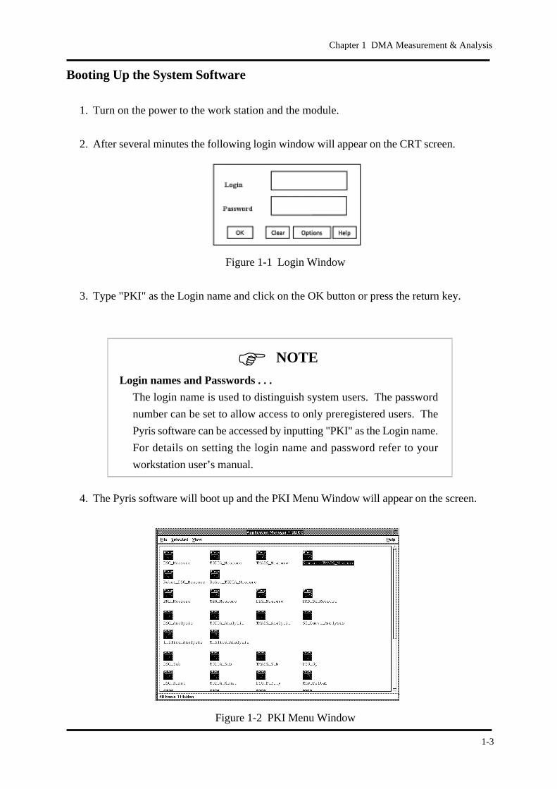
2. After several minutes the following login window will appear on the CRT screen.
Figure 1-1 Login Window
3. Type "PKI" as the Login name and click on the OK button or press the return key.
Login names and Passwords . . .
The login name is used to distinguish system users. The password
number can be set to allow access to only preregistered users. The
Pyris software can be accessed by inputting "PKI" as the Login name.
For details on setting the login name and password refer to your
workstation user’s manual.
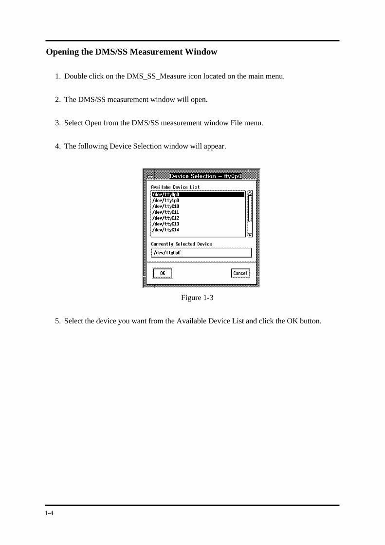
4. The Pyris software will boot up and the PKI Menu Window will appear on the screen.
Figure 1-2 PKI Menu Window
1-4
Opening the DMS/SS Measurement Window
1. Double click on the DMS_SS_Measure icon located on the main menu.
2. The DMS/SS measurement window will open.
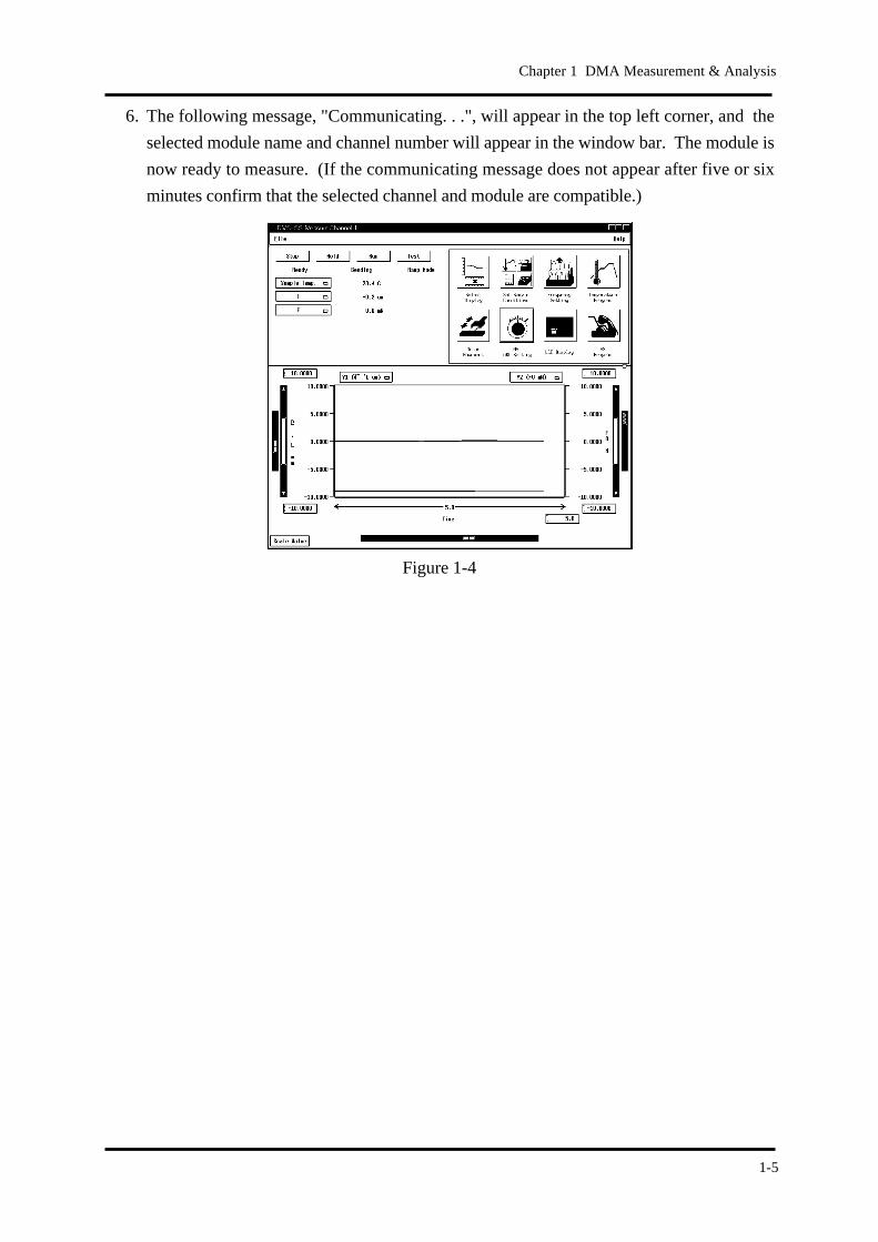
3. Select Open from the DMS/SS measurement window File menu.
4. The following Device Selection window will appear.
Figure 1-3
5. Select the device you want from the Available Device List and click the OK button.
1-5
Chapter 1 DMA Measurement & Analysis
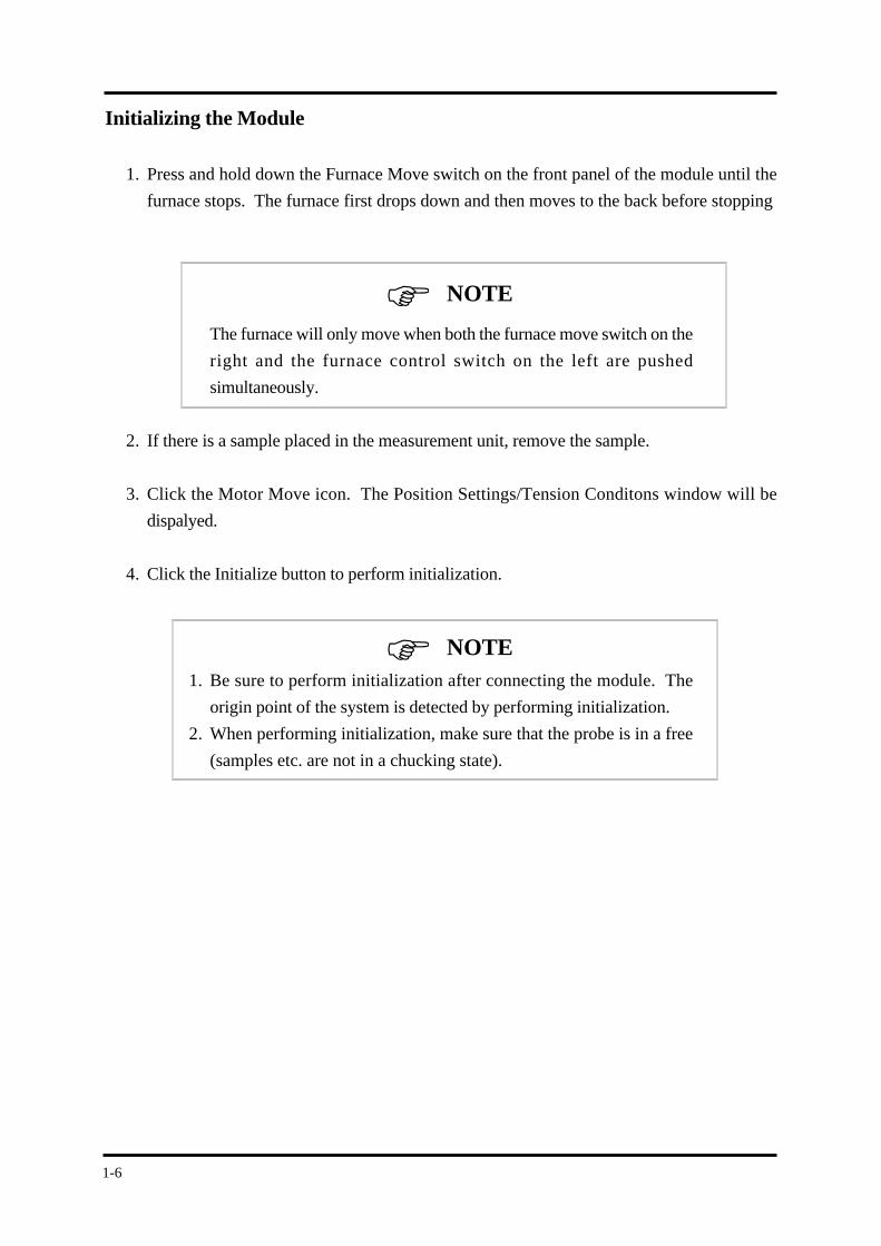
6. The following message, "Communicating. . .", will appear in the top left corner, and the
selected module name and channel number will appear in the window bar. The module is
now ready to measure. (If the communicating message does not appear after five or six
minutes confirm that the selected channel and module are compatible.)
Figure 1-4
1-6
NOTE
Initializing the Module
1. Press and hold down the Furnace Move switch on the front panel of the module until the
furnace stops. The furnace first drops down and then moves to the back before stopping
The furnace will only move when both the furnace move switch on the
right and the furnace control switch on the left are pushed
simultaneously.
2. If there is a sample placed in the measurement unit, remove the sample.
3. Click the Motor Move icon. The Position Settings/Tension Conditons window will be
dispalyed.
4. Click the Initialize button to perform initialization.
1. Be sure to perform initialization after connecting the module. The
origin point of the system is detected by performing initialization.
2. When performing initialization, make sure that the probe is in a free
(samples etc. are not in a chucking state).
NOTE
1-7
Chapter 1 DMA Measurement & Analysis
Information
Information
Attaching Sample Unit Attachments
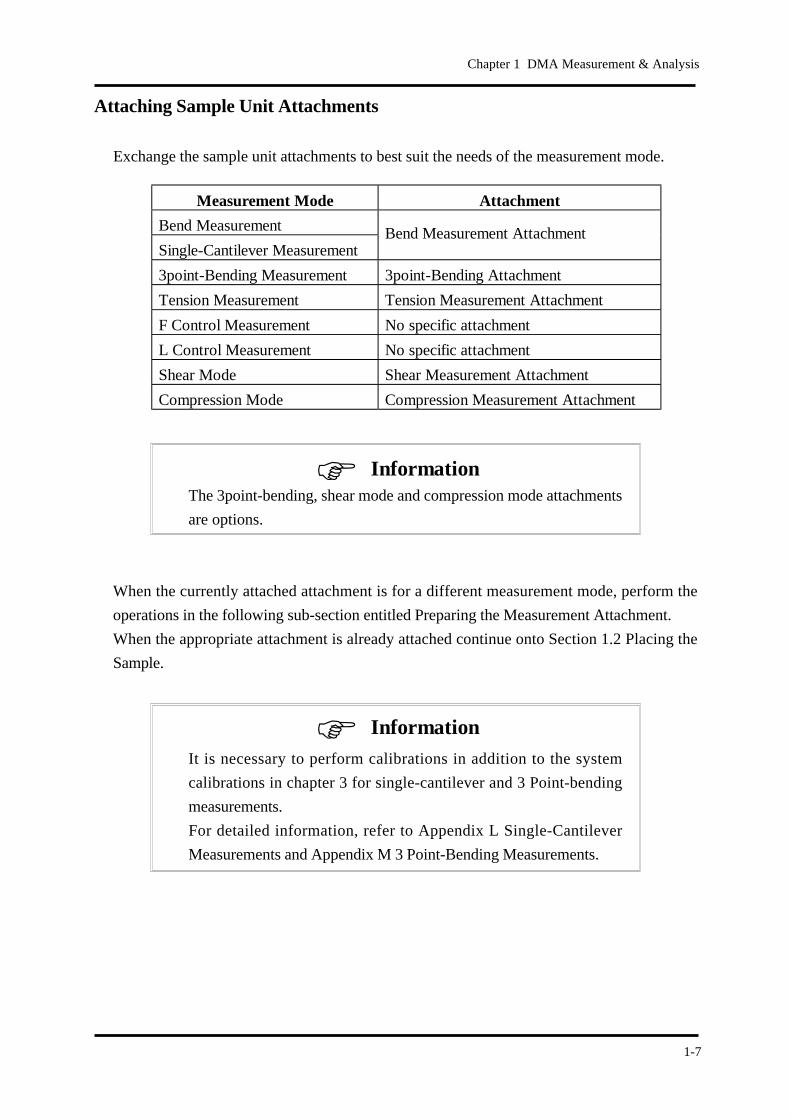
Exchange the sample unit attachments to best suit the needs of the measurement mode.
The 3point-bending, shear mode and compression mode attachments
are options.
When the currently attached attachment is for a different measurement mode, perform the
operations in the following sub-section entitled Preparing the Measurement Attachment.
When the appropriate attachment is already attached continue onto Section 1.2 Placing the
Sample.
It is necessary to perform calibrations in addition to the system
calibrations in chapter 3 for single-cantilever and 3 Point-bending
measurements.
For detailed information, refer to Appendix L Single-Cantilever
Measurements and Appendix M 3 Point-Bending Measurements.
Measurement Mode Attachment
Bend Measurement
Single-Cantilever MeasurementBend Measurement Attachment
3point-Bending Measurement 3point-Bending Attachment
Tension Measurement Tension Measurement Attachment
F Control Measurement No specific attachment
L Control Measurement No specific attachment
Shear Mode Shear Measurement Attachment
Compression Mode Compression Measurement Attachment
1-8
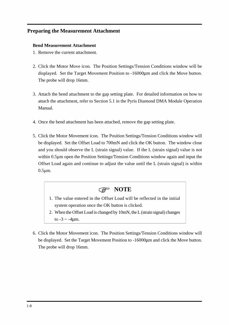
Preparing the Measurement Attachment
Bend Measurement Attachment
1. Remove the current attachment.
2. Click the Motor Move icon. The Position Settings/Tension Conditions window will be
displayed. Set the Target Movement Position to -16000µm and click the Move button.
The probe will drop 16mm.
3. Attach the bend attachment to the gap setting plate. For detailed information on how to
attach the attachment, refer to Section 5.1 in the Pyris Diamond DMA Module Operation
Manual.
4. Once the bend attachment has been attached, remove the gap setting plate.
5. Click the Motor Movement icon. The Position Settings/Tension Conditions window will
be displayed. Set the Offset Load to 700mN and click the OK button. The window close
and you should observe the L (strain signal) value. If the L (strain signal) value is not
within 0.5µm open the Position Settings/Tension Conditions window again and input the
Offset Load again and continue to adjust the value until the L (strain signal) is within
0.5µm.
1. The value entered in the Offset Load will be reflected in the initial
system operation once the OK button is clicked.
2. When the Offset Load is changed by 10mN, the L (strain signal) changes
to -3 ~ -4µm.
6. Click the Motor Movement icon. The Position Settings/Tension Conditions window will
be displayed. Set the Target Movement Position to -16000µm and click the Move button.
The probe will drop 16mm.
NOTE
1-9
Chapter 1 DMA Measurement & Analysis
NOTE
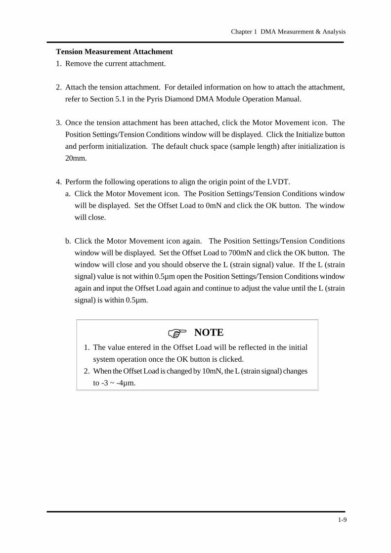
Tension Measurement Attachment
1. Remove the current attachment.
2. Attach the tension attachment. For detailed information on how to attach the attachment,
refer to Section 5.1 in the Pyris Diamond DMA Module Operation Manual.
3. Once the tension attachment has been attached, click the Motor Movement icon. The
Position Settings/Tension Conditions window will be displayed. Click the Initialize button
and perform initialization. The default chuck space (sample length) after initialization is
20mm.
4. Perform the following operations to align the origin point of the LVDT.
a. Click the Motor Movement icon. The Position Settings/Tension Conditions window
will be displayed. Set the Offset Load to 0mN and click the OK button. The window
will close.
b. Click the Motor Movement icon again. The Position Settings/Tension Conditions
window will be displayed. Set the Offset Load to 700mN and click the OK button. The
window will close and you should observe the L (strain signal) value. If the L (strain
signal) value is not within 0.5µm open the Position Settings/Tension Conditions window
again and input the Offset Load again and continue to adjust the value until the L (strain
signal) is within 0.5µm.
1. The value entered in the Offset Load will be reflected in the initial
system operation once the OK button is clicked.
2. When the Offset Load is changed by 10mN, the L (strain signal) changes
to -3 ~ -4µm.
1-10
NOTE
1.2 Placing the SamplePreparation
1. Make the sample into an appropriate shape beforehand. To determine the appropriate
shape, refer to Appendix A and B in the Dynamic Mechanical Analyzer Measurement
Procedure Pyris Diamond DMA Operation Manual.
2. Sample Fusion Protection Operations
When there is a possibility that the measurement sample may attach to the chuck or clamp
during the measurement, apply an anti stick compound. A soapy water solution is a simple
compound to use.
If the sample is the sort that may stick to the measurement head or
chuck, use an anti stick compound before setting the sample.
A sillicon based spray works well.
1-11
Chapter 1 DMA Measurement & Analysis
Information
Placement Method
For Bend Measurements
1. When the chuck is at the origin point, click the Motor Movement icon. The Position
Settings/Tension Conditions window will be displayed. Set the Target Movement Position
to -16000µm and click the Move button. The chuck will drop to the sample set position.
2. Loosen the clamp knurled screws and the chuck hexagonal screws then slide the PMMA
sample from the right through the space between the base and the clamp.
3. Adjust the position of the sample using a pair of tweezers, tighten both of the clamp knurled
screws. Next, align the chuck hexagonal screw and tighten it.
4. Loosen both clamps temporarily, and refasten both clamps. Use the attached flathead
screwdriver fasten.
1. When using soft samples such as rubber type samples, tighten the
chuck side first and then both of the clamps so that the sample does
not bend.
2. When loosening both clamps in step 4, the sample warp that appears
when tightening the chuck screws in step 3 is elminated.
1-12
Information
NOTE
For Tension Measurements
1. Enter a value in µm units into the Movement Target Position and click the Move button.
When Move is clicked, the stage motor position moves to the target position.
The standard length for the samples is 20mm. Therefore, when
measuring samples with lengths of 20mm the Movement Target
Position is 0µm. When the sample length is 10mm enter -10000 for
the Movement Target Position and enter 5000 for a sample length of
25mm then click the Move button.
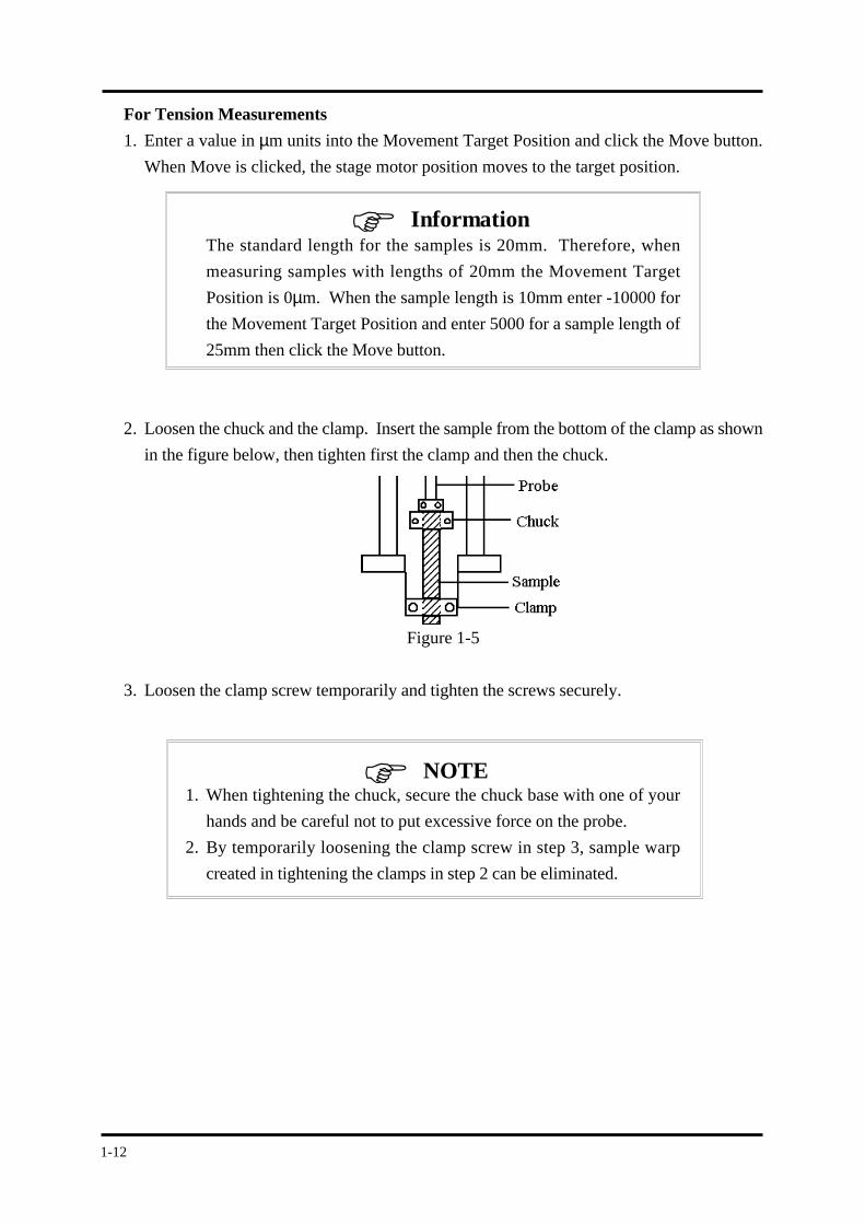
2. Loosen the chuck and the clamp. Insert the sample from the bottom of the clamp as shown
in the figure below, then tighten first the clamp and then the chuck.
Figure 1-5
3. Loosen the clamp screw temporarily and tighten the screws securely.
1. When tightening the chuck, secure the chuck base with one of your
hands and be careful not to put excessive force on the probe.
2. By temporarily loosening the clamp screw in step 3, sample warp
created in tightening the clamps in step 2 can be eliminated.
1-13
Chapter 1 DMA Measurement & Analysis
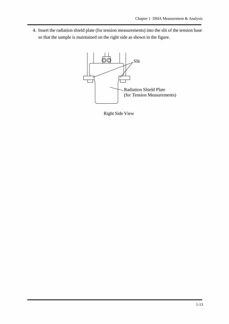
4. Insert the radiation shield plate (for tension measurements) into the slit of the tension base
so that the sample is maintained on the right side as shown in the figure.
Right Side View
Radiation Shield Plate(for Tension Measurements)
Slit
1-14
Information
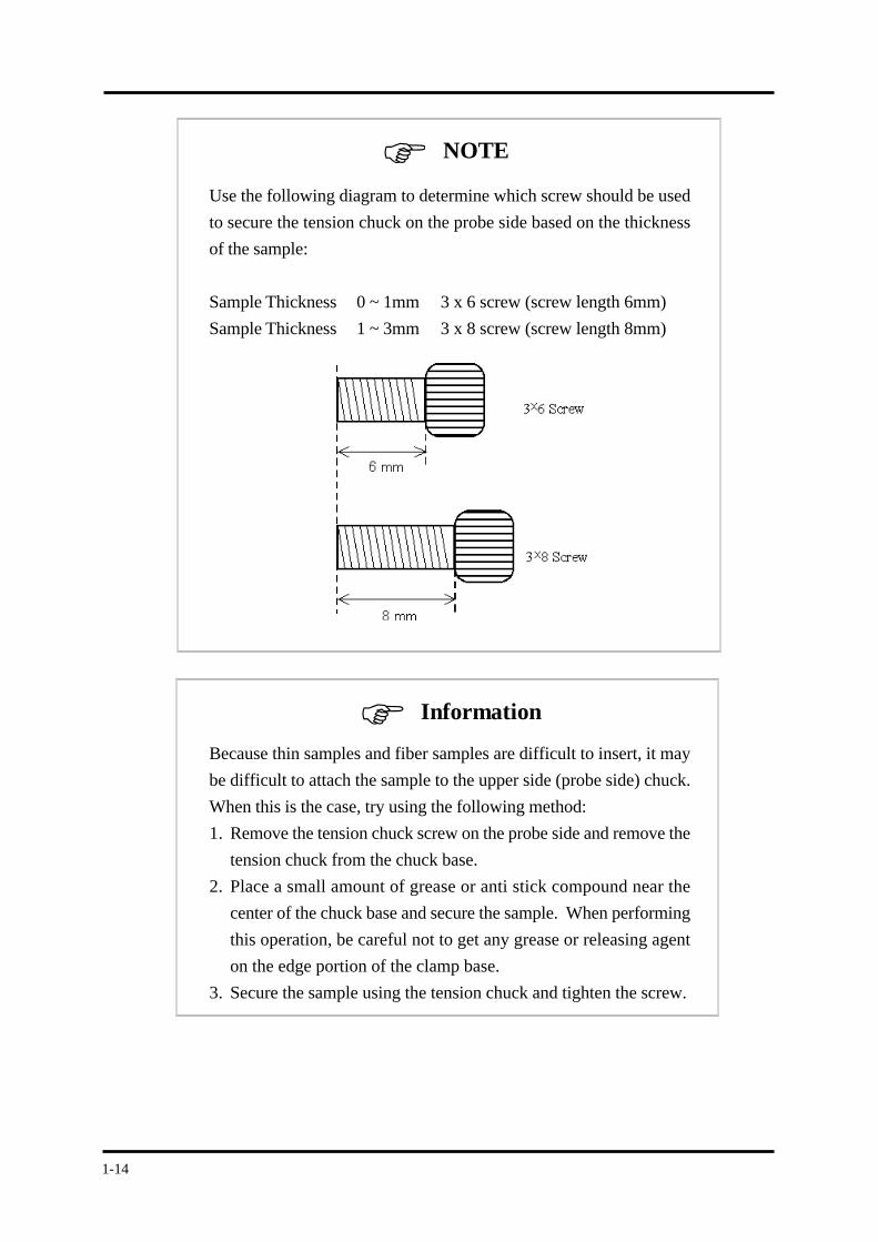
Use the following diagram to determine which screw should be used
to secure the tension chuck on the probe side based on the thickness
of the sample:
Sample Thickness 0 ~ 1mm 3 x 6 screw (screw length 6mm)
Sample Thickness 1 ~ 3mm 3 x 8 screw (screw length 8mm)
Because thin samples and fiber samples are difficult to insert, it may
be difficult to attach the sample to the upper side (probe side) chuck.
When this is the case, try using the following method:
1. Remove the tension chuck screw on the probe side and remove the
tension chuck from the chuck base.
2. Place a small amount of grease or anti stick compound near the
center of the chuck base and secure the sample. When performing
this operation, be careful not to get any grease or releasing agent
on the edge portion of the clamp base.
3. Secure the sample using the tension chuck and tighten the screw.
NOTE
1-15
Chapter 1 DMA Measurement & Analysis
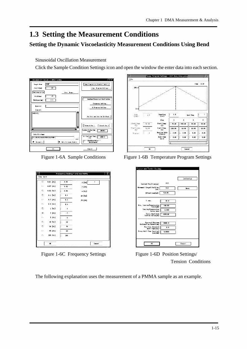
1.3 Setting the Measurement ConditionsSetting the Dynamic Viscoelasticity Measurement Conditions Using Bend
Sinusoidal Oscillation Measurement
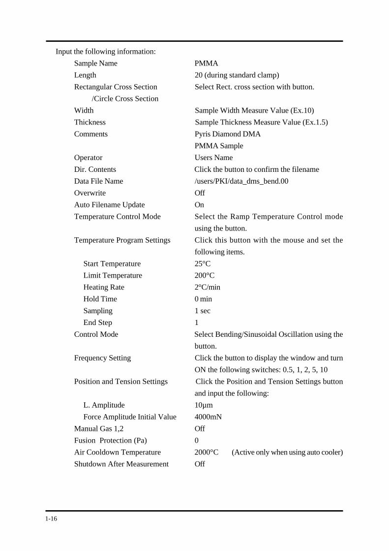
Click the Sample Condition Settings icon and open the window the enter data into each section.
Figure 1-6A Sample Conditions Figure 1-6B Temperature Program Settings
Figure 1-6C Frequency Settings Figure 1-6D Position Settings/
Tension Conditions
The following explanation uses the measurement of a PMMA sample as an example.
1-16
Input the following information:
Sample Name PMMA
Length 20 (during standard clamp)
Rectangular Cross Section Select Rect. cross section with button.
/Circle Cross Section
Width Sample Width Measure Value (Ex.10)
Thickness Sample Thickness Measure Value (Ex.1.5)
Comments Pyris Diamond DMA
PMMA Sample
Operator Users Name
Dir. Contents Click the button to confirm the filename
Data File Name /users/PKI/data_dms_bend.00
Overwrite Off
Auto Filename Update On
Temperature Control Mode Select the Ramp Temperature Control mode
using the button.
Temperature Program Settings Click this button with the mouse and set the
following items.
Start Temperature 25°C
Limit Temperature 200°C
Heating Rate 2°C/min
Hold Time 0 min
Sampling 1 sec
End Step 1
Control Mode Select Bending/Sinusoidal Oscillation using the
button.
Frequency Setting Click the button to display the window and turn
ON the following switches: 0.5, 1, 2, 5, 10
Position and Tension Settings Click the Position and Tension Settings button
and input the following:
L. Amplitude 10µm
Force Amplitude Initial Value 4000mN
Manual Gas 1,2 Off
Fusion Protection (Pa) 0
Air Cooldown Temperature 2000°C (Active only when using auto cooler)
Shutdown After Measurement Off
1-17
Chapter 1 DMA Measurement & Analysis
NOTE1. Temperature program settings can also be modified through the
Temperature Program icon.
2. Frequency settings can also be modified through the Frequency Setting
icon.
3. To measure a sample using the same conditions you only need to
enter the sample name and shape.
4. When all of the Frequency Settings are Off, the default setting of 2Hz
will be used.
5. When measuring soft samples, set the Force Amplitude Initial Value
to a low setting. (ex. 10mN)
1-18
NOTE
Synthetic Oscillation Measurement
For the synthetic oscillation measurement, make the following changes to the previous settings
for the sinusoidal oscillation measurement:
Comments Sinusoidal Oscillation → Synthetic Oscillation
Control Mode Bending/Synthetic oscillation mode.
Frequency Setting Click the button to display the window and enter
0.5 (Hz) for the standard frequency section of
right side.
L. Amplitude 10 → 5
The L. Amplitude (target) for the Synthetic Oscillation measurement
is relative to the standard frequency used. During the measurement,
the actual L. Amplitude is comprised of each of the frequency
components so the amplitude should be as close to 5 times the target
value as possible. For Synthetic Oscillation measurements, the L.
Amplitude should generally be set to 5µm.
1-19
Chapter 1 DMA Measurement & Analysis
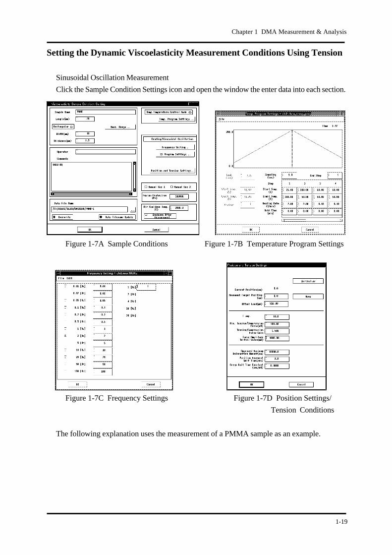
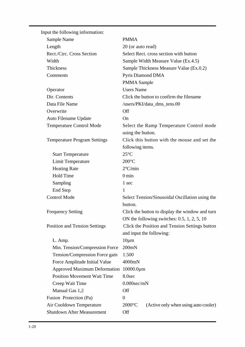
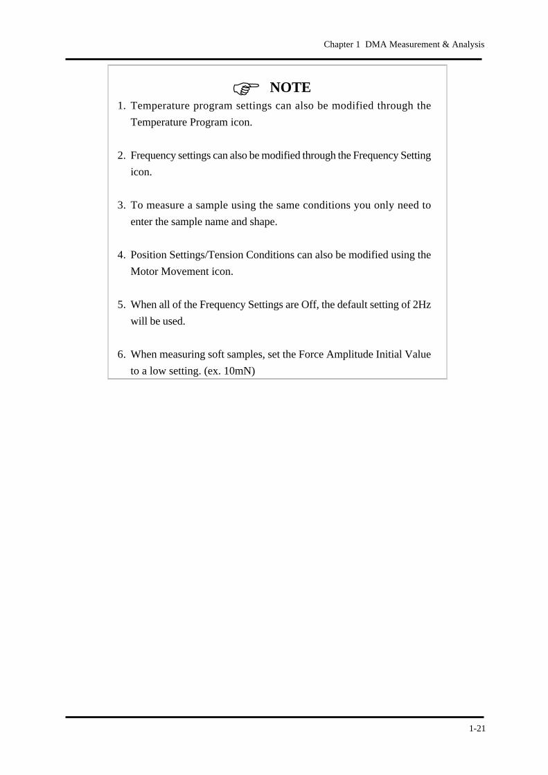
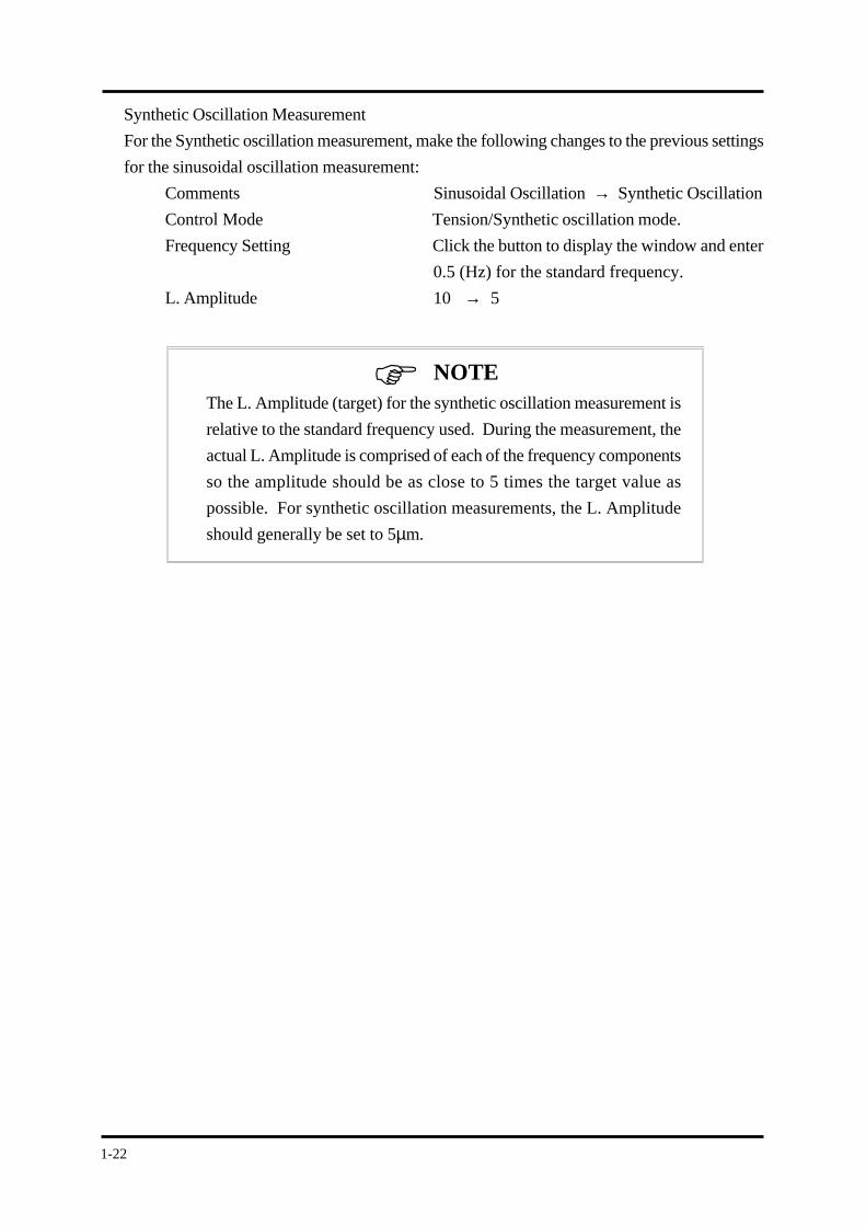
Setting the Dynamic Viscoelasticity Measurement Conditions Using Tension
Sinusoidal Oscillation Measurement
Click the Sample Condition Settings icon and open the window the enter data into each section.
Figure 1-7A Sample Conditions Figure 1-7B Temperature Program Settings
Figure 1-7C Frequency Settings Figure 1-7D Position Settings/
Tension Conditions
The following explanation uses the measurement of a PMMA sample as an example.
1-20
Input the following information:
Sample Name PMMA
Length 20 (or auto read)
Rect./Circ. Cross Section Select Rect. cross section with button
Width Sample Width Measure Value (Ex.4.5)
Thickness Sample Thickness Measure Value (Ex.0.2)
Comments Pyris Diamond DMA
PMMA Sample
Operator Users Name
Dir. Contents Click the button to confirm the filename
Data File Name /users/PKI/data_dms_tens.00
Overwrite Off
Auto Filename Update On
Temperature Control Mode Select the Ramp Temperature Control mode
using the button.
Temperature Program Settings Click this button with the mouse and set the
following items.
Start Temperature 25°C
Limit Temperature 200°C
Heating Rate 2°C/min
Hold Time 0 min
Sampling 1 sec
End Step 1
Control Mode Select Tension/Sinusoidal Oscillation using the
button.
Frequency Setting Click the button to display the window and turn
ON the following switches: 0.5, 1, 2, 5, 10
Position and Tension Settings Click the Position and Tension Settings button
and input the following:
L. Amp. 10µm
Min. Tension/Compression Force 200mN
Tension/Compression Force gain 1.500
Force Amplitude Initial Value 4000mN
Approved Maximum Deformation 10000.0µm
Position Movement Wait Time 8.0sec
Creep Wait Time 0.000sec/mN
Manual Gas 1,2 Off
Fusion Protection (Pa) 0
Air Cooldown Temperature 2000°C (Active only when using auto cooler)
Shutdown After Measurement Off
1-21
Chapter 1 DMA Measurement & Analysis
NOTE1. Temperature program settings can also be modified through the
Temperature Program icon.
2. Frequency settings can also be modified through the Frequency Setting
icon.
3. To measure a sample using the same conditions you only need to
enter the sample name and shape.
4. Position Settings/Tension Conditions can also be modified using the
Motor Movement icon.
5. When all of the Frequency Settings are Off, the default setting of 2Hz
will be used.
6. When measuring soft samples, set the Force Amplitude Initial Value
to a low setting. (ex. 10mN)
1-22
NOTE
Synthetic Oscillation Measurement
For the Synthetic oscillation measurement, make the following changes to the previous settings
for the sinusoidal oscillation measurement:
Comments Sinusoidal Oscillation → Synthetic Oscillation
Control Mode Tension/Synthetic oscillation mode.
Frequency Setting Click the button to display the window and enter
0.5 (Hz) for the standard frequency.
L. Amplitude 10 → 5
The L. Amplitude (target) for the synthetic oscillation measurement is
relative to the standard frequency used. During the measurement, the
actual L. Amplitude is comprised of each of the frequency components
so the amplitude should be as close to 5 times the target value as
possible. For synthetic oscillation measurements, the L. Amplitude
should generally be set to 5µm.
1-23
Chapter 1 DMA Measurement & Analysis
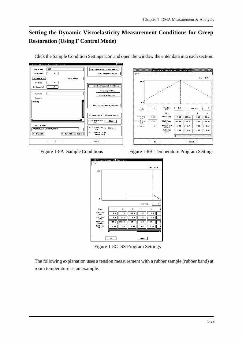
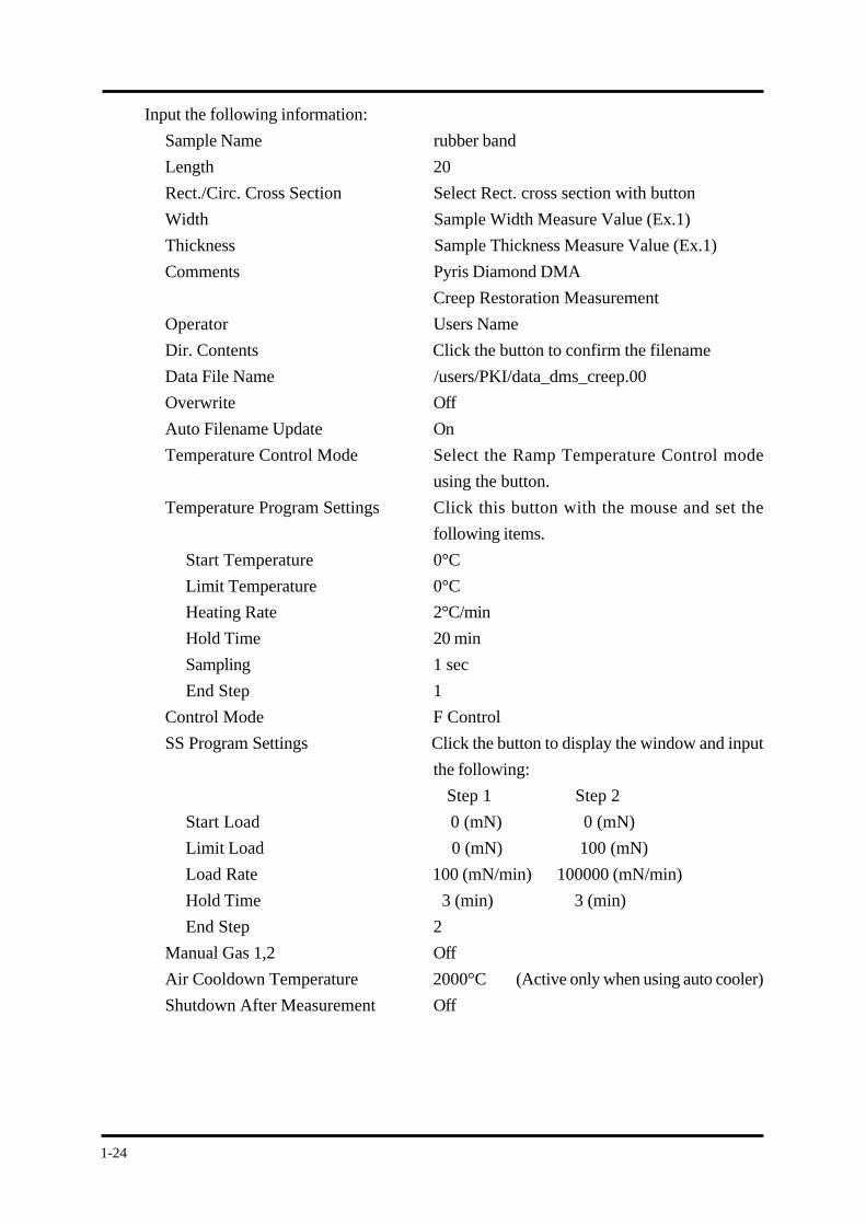
Setting the Dynamic Viscoelasticity Measurement Conditions for Creep
Restoration (Using F Control Mode)
Click the Sample Condition Settings icon and open the window the enter data into each section.
Figure 1-8A Sample Conditions Figure 1-8B Temperature Program Settings
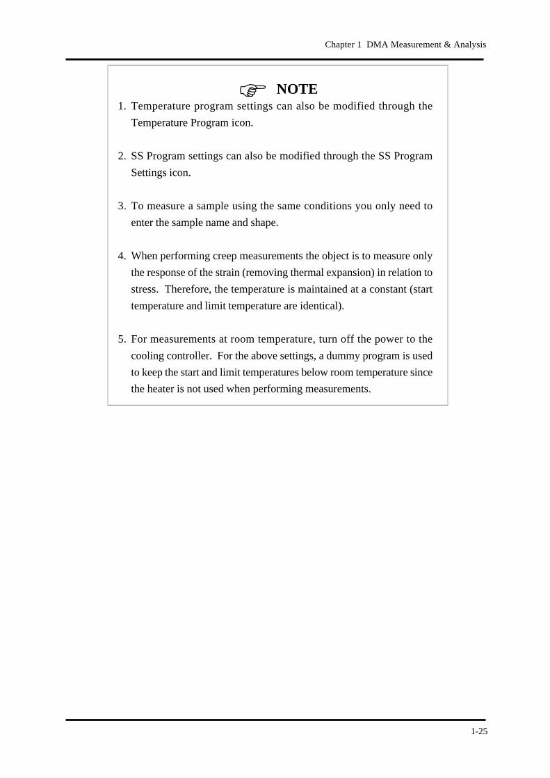
Figure 1-8C SS Program Settings
The following explanation uses a tension measurement with a rubber sample (rubber band) at
room temperature as an example.
1-24
Input the following information:
Sample Name rubber band
Length 20
Rect./Circ. Cross Section Select Rect. cross section with button
Width Sample Width Measure Value (Ex.1)
Thickness Sample Thickness Measure Value (Ex.1)
Comments Pyris Diamond DMA
Creep Restoration Measurement
Operator Users Name
Dir. Contents Click the button to confirm the filename
Data File Name /users/PKI/data_dms_creep.00
Overwrite Off
Auto Filename Update On
Temperature Control Mode Select the Ramp Temperature Control mode
using the button.
Temperature Program Settings Click this button with the mouse and set the
following items.
Start Temperature 0°C
Limit Temperature 0°C
Heating Rate 2°C/min
Hold Time 20 min
Sampling 1 sec
End Step 1
Control Mode F Control
SS Program Settings Click the button to display the window and input
the following:
Step 1 Step 2
Start Load 0 (mN) 0 (mN)
Limit Load 0 (mN) 100 (mN)
Load Rate 100 (mN/min) 100000 (mN/min)
Hold Time 3 (min) 3 (min)
End Step 2
Manual Gas 1,2 Off
Air Cooldown Temperature 2000°C (Active only when using auto cooler)
Shutdown After Measurement Off
1-25
Chapter 1 DMA Measurement & Analysis
NOTE1. Temperature program settings can also be modified through the
Temperature Program icon.
2. SS Program settings can also be modified through the SS Program
Settings icon.
3. To measure a sample using the same conditions you only need to
enter the sample name and shape.
4. When performing creep measurements the object is to measure only
the response of the strain (removing thermal expansion) in relation to
stress. Therefore, the temperature is maintained at a constant (start
temperature and limit temperature are identical).
5. For measurements at room temperature, turn off the power to the
cooling controller. For the above settings, a dummy program is used
to keep the start and limit temperatures below room temperature since
the heater is not used when performing measurements.
1-26
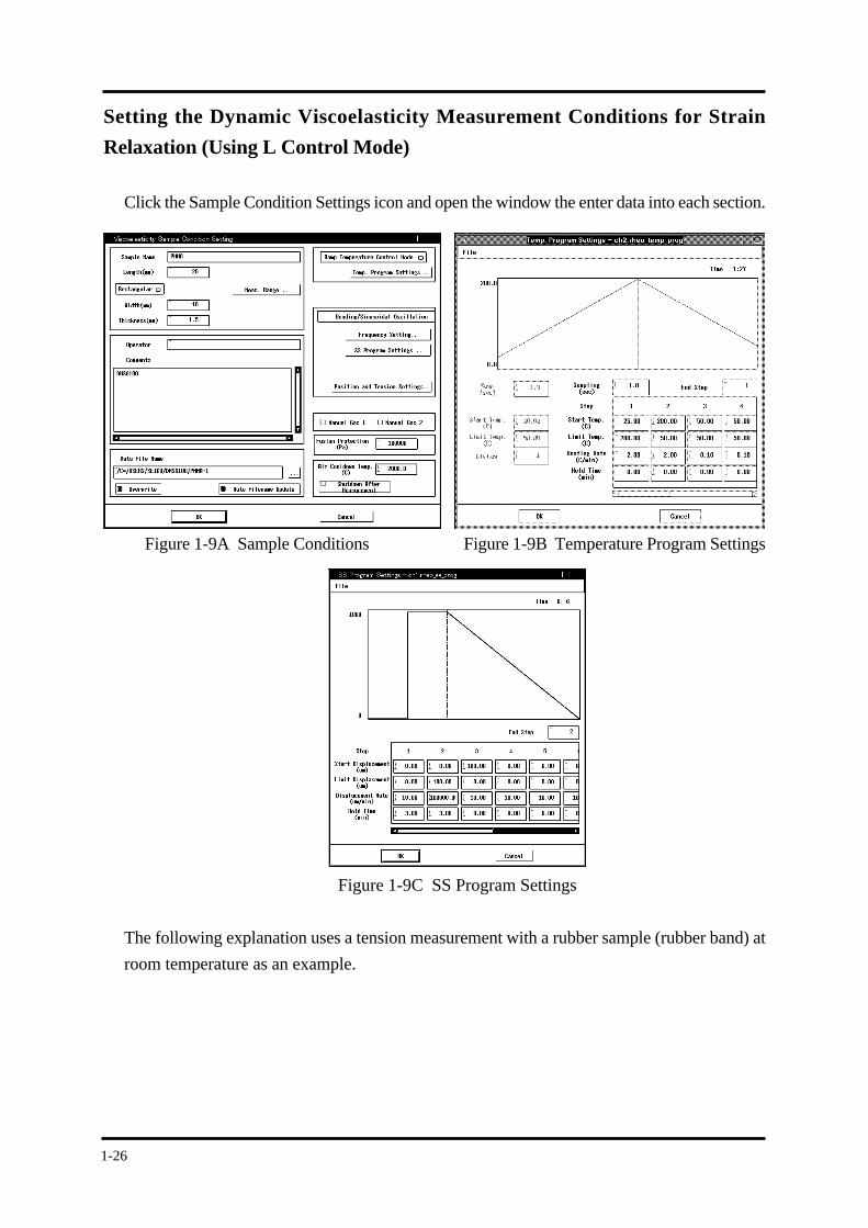
Setting the Dynamic Viscoelasticity Measurement Conditions for Strain
Relaxation (Using L Control Mode)
Click the Sample Condition Settings icon and open the window the enter data into each section.
Figure 1-9A Sample Conditions Figure 1-9B Temperature Program Settings
Figure 1-9C SS Program Settings
The following explanation uses a tension measurement with a rubber sample (rubber band) at
room temperature as an example.
1-27
Chapter 1 DMA Measurement & Analysis
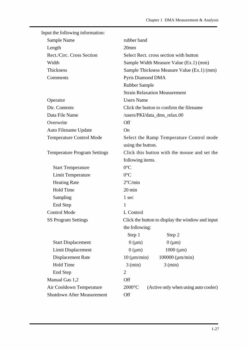
Input the following information:
Sample Name rubber band
Length 20mm
Rect./Circ. Cross Section Select Rect. cross section with button
Width Sample Width Measure Value (Ex.1) (mm)
Thickness Sample Thickness Measure Value (Ex.1) (mm)
Comments Pyris Diamond DMA
Rubber Sample
Strain Relaxation Measurement
Operator Users Name
Dir. Contents Click the button to confirm the filename
Data File Name /users/PKI/data_dms_relax.00
Overwrite Off
Auto Filename Update On
Temperature Control Mode Select the Ramp Temperature Control mode
using the button.
Temperature Program Settings Click this button with the mouse and set the
following items.
Start Temperature 0°C
Limit Temperature 0°C
Heating Rate 2°C/min
Hold Time 20 min
Sampling 1 sec
End Step 1
Control Mode L Control
SS Program Settings Click the button to display the window and input
the following:
Step 1 Step 2
Start Displacement 0 (µm) 0 (µm)
Limit Displacement 0 (µm) 1000 (µm)
Displacement Rate 10 (µm/min) 100000 (µm/min)
Hold Time 3 (min) 3 (min)
End Step 2
Manual Gas 1,2 Off
Air Cooldown Temperature 2000°C (Active only when using auto cooler)
Shutdown After Measurement Off
1-28
NOTE
1. Temperature program settings can also be modified through the
Temperature Program icon.
2. SS Program settings can also be modified through the SS Program
Settings icon.
3. To measure a sample using the same conditions you only need to
enter the sample name and shape.
4. When performing stress relaxation measurements the object is to
measure only the stress changes by controlling the amplitude
rectangularly. Therefore, the temperature is maintained at a constant
(start temperature and limit temperature are identical).
5. For measurements at room temperature, turn off the power to the
cooling controller. For the above settings, a dummy program is used
to keep the start and limit temperatures below room temperature since
the heater is not used when performing measurements.
1-29
Chapter 1 DMA Measurement & Analysis
1.4 Starting and Stopping MeasurementsFor Sinusoidal and Synthetic Osciallation Modes
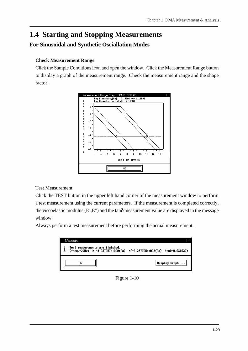
Check Measurement Range
Click the Sample Conditions icon and open the window. Click the Measurement Range button
to display a graph of the measurement range. Check the measurement range and the shape
factor.
Test Measurement
Click the TEST button in the upper left hand corner of the measurement window to perform
a test measurement using the current parameters. If the measurement is completed correctly,
the viscoelastic modulus (E’,E”) and the tanδ measurement value are displayed in the message
window.
Always perform a test measurement before performing the actual measurement.
Figure 1-10
1-30
NOTE
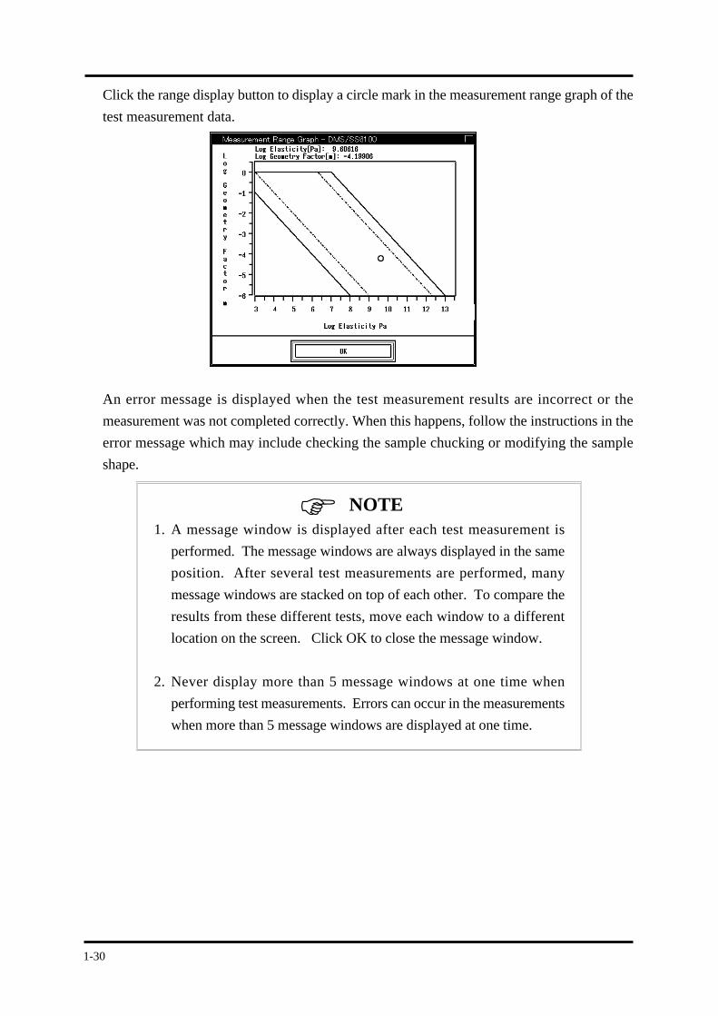
Click the range display button to display a circle mark in the measurement range graph of the
test measurement data.
An error message is displayed when the test measurement results are incorrect or the
measurement was not completed correctly. When this happens, follow the instructions in the
error message which may include checking the sample chucking or modifying the sample
shape.
1. A message window is displayed after each test measurement is
performed. The message windows are always displayed in the same
position. After several test measurements are performed, many
message windows are stacked on top of each other. To compare the
results from these different tests, move each window to a different
location on the screen. Click OK to close the message window.
2. Never display more than 5 message windows at one time when
performing test measurements. Errors can occur in the measurements
when more than 5 message windows are displayed at one time.
1-31
Chapter 1 DMA Measurement & Analysis
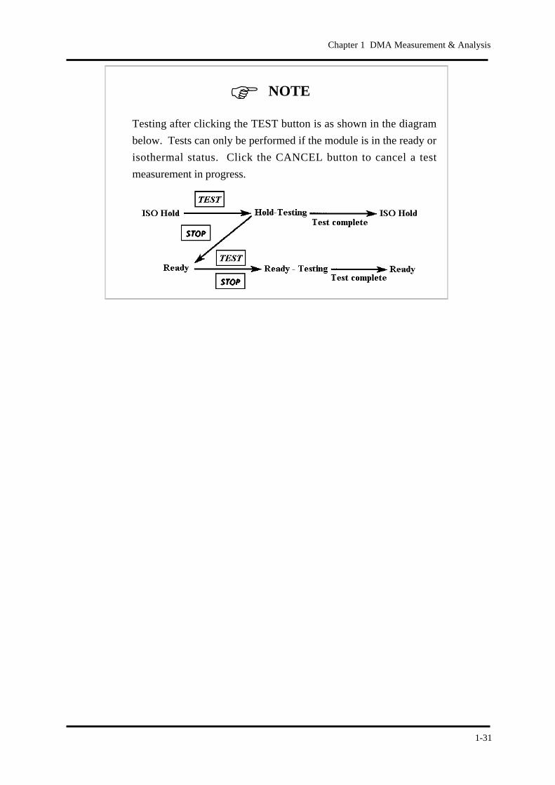
Testing after clicking the TEST button is as shown in the diagram
below. Tests can only be performed if the module is in the ready or
isothermal status. Click the CANCEL button to cancel a test
measurement in progress.
NOTE
1-32
NOTE
Starting and Stopping Measurements
The four module control buttons are located in the upper left hand side of the window. When
one of these buttons is pushed the module will follow the temperature program settings and
control the temperature.
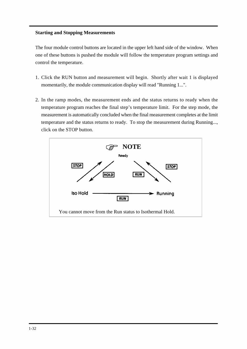
1. Click the RUN button and measurement will begin. Shortly after wait 1 is displayed
momentarily, the module communication display will read "Running 1...".
2. In the ramp modes, the measurement ends and the status returns to ready when the
temperature program reaches the final step’s temperature limit. For the step mode, the
measurement is automatically concluded when the final measurement completes at the limit
temperature and the status returns to ready. To stop the measurement during Running...,
click on the STOP button.
You cannot move from the Run status to Isothermal Hold.
1-33
Chapter 1 DMA Measurement & Analysis
NOTE
F, L Control Modes
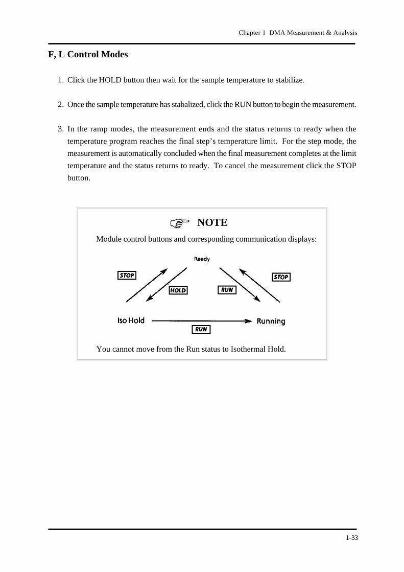
1. Click the HOLD button then wait for the sample temperature to stabilize.
2. Once the sample temperature has stabalized, click the RUN button to begin the measurement.
3. In the ramp modes, the measurement ends and the status returns to ready when the
temperature program reaches the final step’s temperature limit. For the step mode, the
measurement is automatically concluded when the final measurement completes at the limit
temperature and the status returns to ready. To cancel the measurement click the STOP
button.
Module control buttons and corresponding communication displays:
You cannot move from the Run status to Isothermal Hold.

1-34
NOTE
Control Target During L Control
L Control mode operates the step motor, moves the detector position up and down and
introduces it into the stage.
Along with the movement of the stage, the probe moves up and down and the sample length
changes in accordance with the L Program.
The stage is controlled by the following equation during the L control measurement:
Stage Position = Movement Target Position (the last place moved to using the Move button
in the Motor Movement icon) + L Control Program Value (in the SS
Program icon)
In other words, during the L Control Measurement, the stage moves only the output value of
the L Program with the last used movement position set to 0µm.
The stage does not move in the Ready status.
The stage movement origin point at the L Program control is the last
used movement position and not the current position. Furthermore, if
the space between the last used movement target position and the
current position is too large, the stage moves large distance along
with the starting of the L control setting.
To avoid this, use the Move button in the Motor Move icon before
the measurement and move the stage to the desired position. By
performing this operation, the current and target positions will be the
same and the above problem will not occur.
1-35
Chapter 1 DMA Measurement & Analysis
NOTE
Parameter Precalibration and Initialization with Control Loop
There are several parameters to be set within the control loop. In order to measure a variety
of samples using viscoelastic measurements, these parameters precalibrate the sample properties
while continuing measurements. This is known as the precalibration feature.
This precalibration feature is extremely effective for continuous samples with viscoelastic
changes but when the sample is exchanged and the sample materials change, measurement
errors can occur causing an obstacle to measurements.
In this circumstance, use the method below to perform initialization of the updated control
parameters for each control mode.
1. All Sinusoidal and Synthetic Oscillation Modes
Click the TEST button in the upper left corner of the measurement window and perform a
TEST measurement. The control parameters are initialized.
2. F Control Mode
To initialize the control parameters move to the sinoidal wave or synthetic wave, perform
a test measurement, then return to the F control mode.
3. L control Mode
To initialize the control parameters move to the sinusoidal oscillation or synthetic oscillation,
perform a test measurement, then return to the L control mode.
To move to a different control mode, select the other control mode
using the control mode selection button and click the OK button. It is
necessary to confirm the selected control mode.
1-36
Helpful hints . . .
Set measurement mode display
The following should normally be displayed below the buttons in the upper left of the module
control window:
• Current module status (Isothermal Hold, Running, etc.)
• Deformation Mode (Bend, Shear, Tension, Compression, F, L)
• Temperature Mode (Ramp, Step)
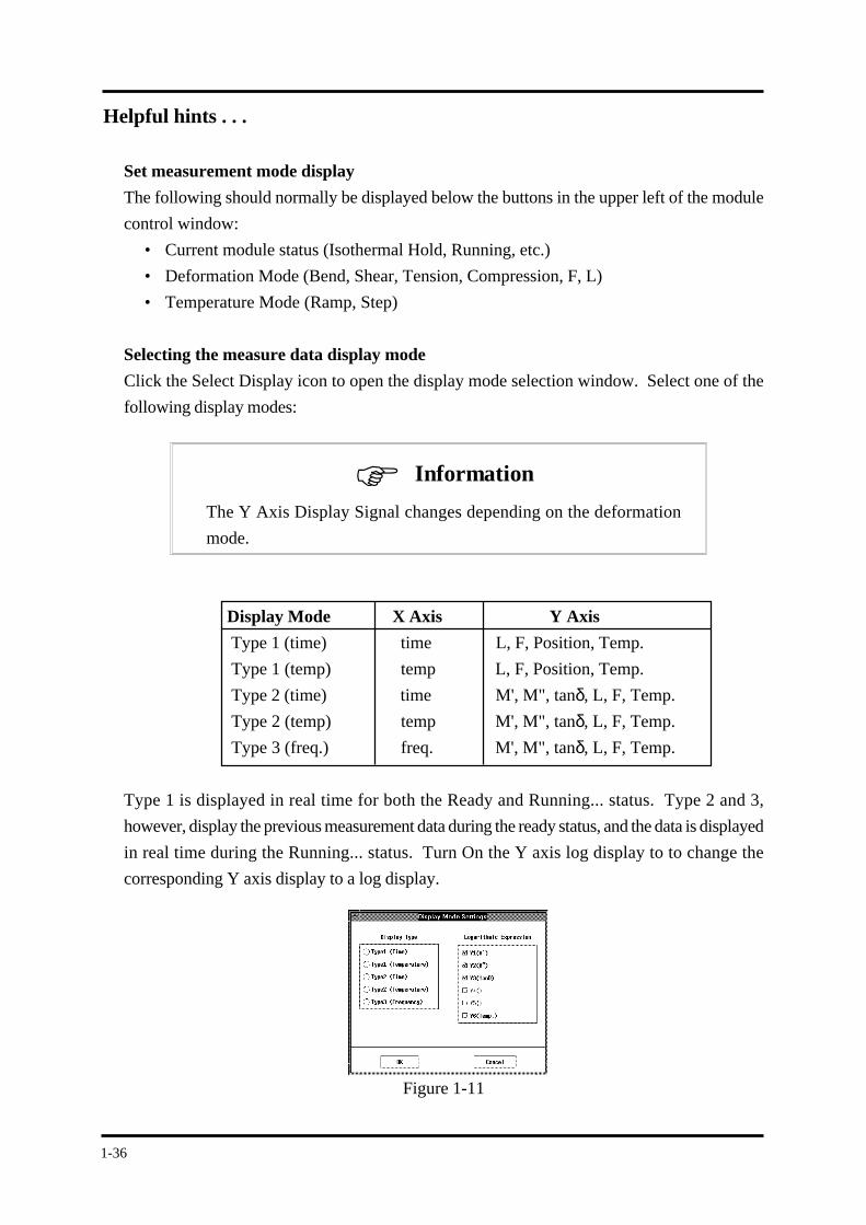
Selecting the measure data display mode
Click the Select Display icon to open the display mode selection window. Select one of the
following display modes:
The Y Axis Display Signal changes depending on the deformation
mode.
Display Mode X Axis Y Axis
Type 1 (time) time L, F, Position, Temp.
Type 1 (temp) temp L, F, Position, Temp.
Type 2 (time) time M', M", tanδ, L, F, Temp.
Type 2 (temp) temp M', M", tanδ, L, F, Temp.
Type 3 (freq.) freq. M', M", tanδ, L, F, Temp.
Type 1 is displayed in real time for both the Ready and Running... status. Type 2 and 3,
however, display the previous measurement data during the ready status, and the data is displayed
in real time during the Running... status. Turn On the Y axis log display to to change the
corresponding Y axis display to a log display.
Figure 1-11
Information
1-37
Chapter 1 DMA Measurement & Analysis
Changing the number of Y-axis displayed
Click on either the Y1 axis or Y2 axis signal setting button to change the axis signal setting.
Select All Y Axes to display all Y1 ~ Y4 set signals.
Enlarging or reducing the data display
Data can be enlarged or reduced using the scroll bars and sliders that accompany each axis.
Data can also be modified using the Scale Value button located in the bottom left hand corner
of the screen.
1-38
1.5 Analyzing Measurement Data
(Sinusoidal & Synthetic Oscillation Control Mode Data)
The data measured with the DMA module can be graphed with time, temperature, or frequency
on the horizontal axis, and with E’, E’’, |E*| , J’, J’’, tanδ, η etc. on the vertical axis, then
analyzed with the analysis job.
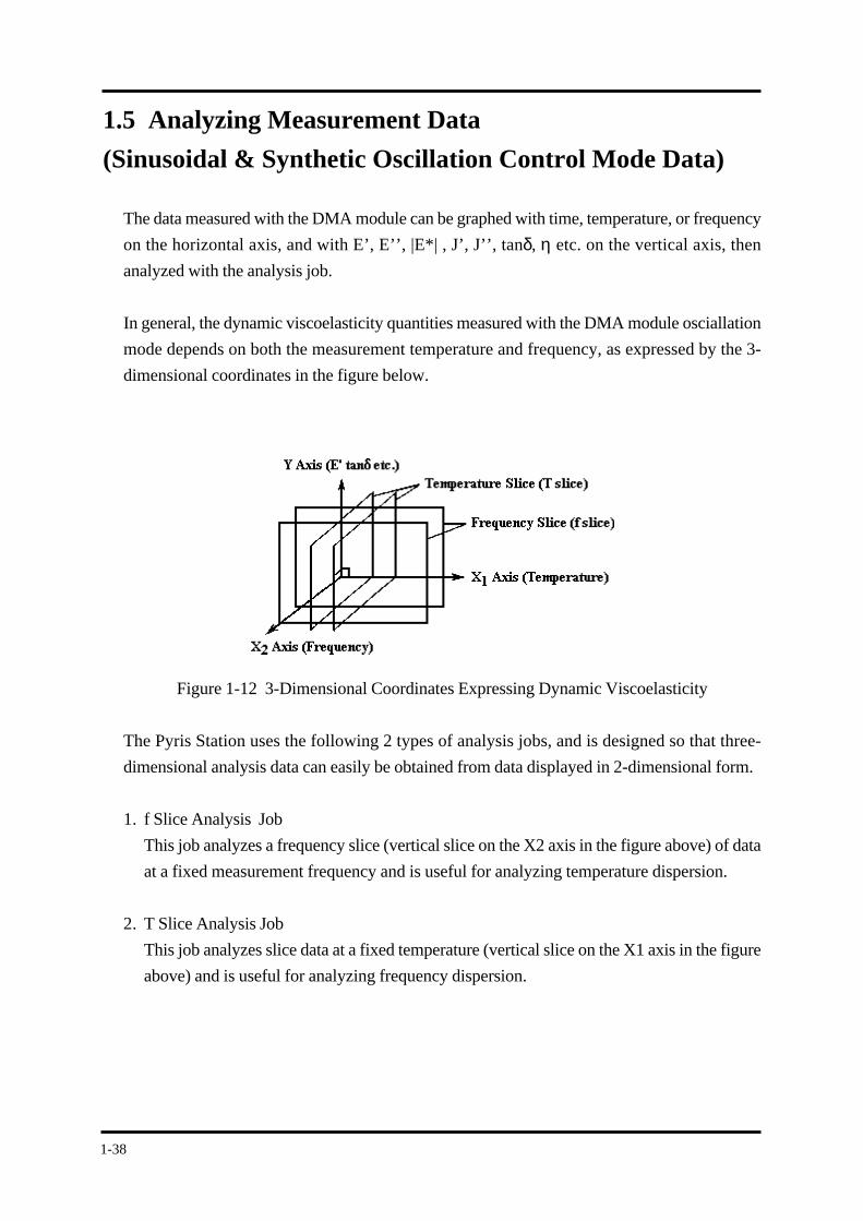
In general, the dynamic viscoelasticity quantities measured with the DMA module osciallation
mode depends on both the measurement temperature and frequency, as expressed by the 3-
dimensional coordinates in the figure below.
Figure 1-12 3-Dimensional Coordinates Expressing Dynamic Viscoelasticity
The Pyris Station uses the following 2 types of analysis jobs, and is designed so that three-
dimensional analysis data can easily be obtained from data displayed in 2-dimensional form.
1. f Slice Analysis Job
This job analyzes a frequency slice (vertical slice on the X2 axis in the figure above) of data
at a fixed measurement frequency and is useful for analyzing temperature dispersion.
2. T Slice Analysis Job
This job analyzes slice data at a fixed temperature (vertical slice on the X1 axis in the figure
above) and is useful for analyzing frequency dispersion.
1-39
Chapter 1 DMA Measurement & Analysis
NOTE
Opening the DMA Analysis Window
1. Double click on the f_Slice_Analysis or T_Slice_Analysis icon found in the PKI main menu
window. (The following explanation will be based on the f slice analysis.)
2. The Slice Analysis window will open.
3. Analysis data has not been selected at this point so all items in the menu bar will be deactivated
except for Open.
4. Select Open from the menu bar and an Open File window will open.
5. Select the target file you want to analyze from the file list
(for example: /users/PKI/data_dms.00) and click the OK button.
When a file containing analyzed results is selected with the mouse, a
data profile will be displayed in the panel located at the right of the file
list.
6. The data is opened and displayed in the window and analysis can begin.
1-40
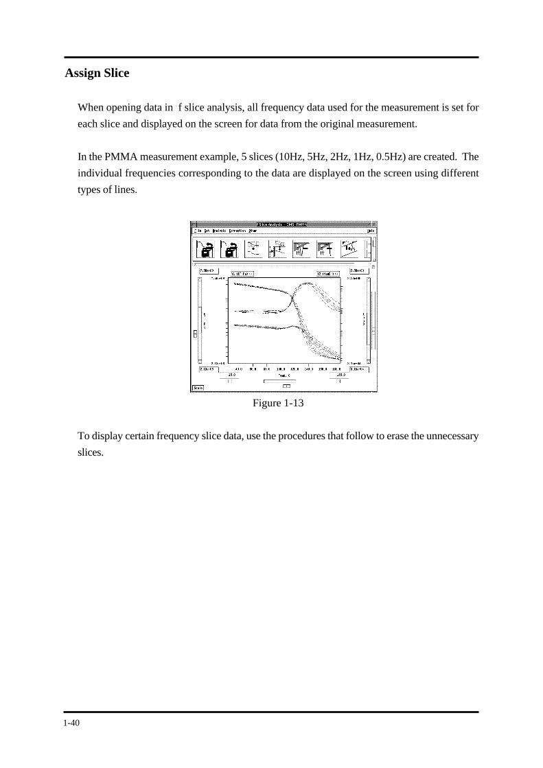
Assign Slice
When opening data in f slice analysis, all frequency data used for the measurement is set for
each slice and displayed on the screen for data from the original measurement.
In the PMMA measurement example, 5 slices (10Hz, 5Hz, 2Hz, 1Hz, 0.5Hz) are created. The
individual frequencies corresponding to the data are displayed on the screen using different
types of lines.
Figure 1-13
To display certain frequency slice data, use the procedures that follow to erase the unnecessary
slices.
1-41
Chapter 1 DMA Measurement & Analysis
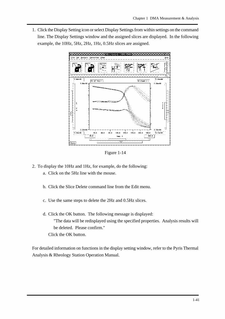
1. Click the Display Setting icon or select Display Settings from within settings on the command
line. The Display Settings window and the assigned slices are displayed. In the following
example, the 10Hz, 5Hz, 2Hz, 1Hz, 0.5Hz slices are assigned.
Figure 1-14
2. To display the 10Hz and 1Hz, for example, do the following:
a. Click on the 5Hz line with the mouse.
b. Click the Slice Delete command line from the Edit menu.
c. Use the same steps to delete the 2Hz and 0.5Hz slices.
d. Click the OK button. The following message is displayed:
"The data will be redisplayed using the specified properties. Analysis results will
be deleted. Please confirm."
Click the OK button.
For detailed information on functions in the display setting window, refer to the Pyris Thermal
Analysis & Rheology Station Operation Manual.
1-42
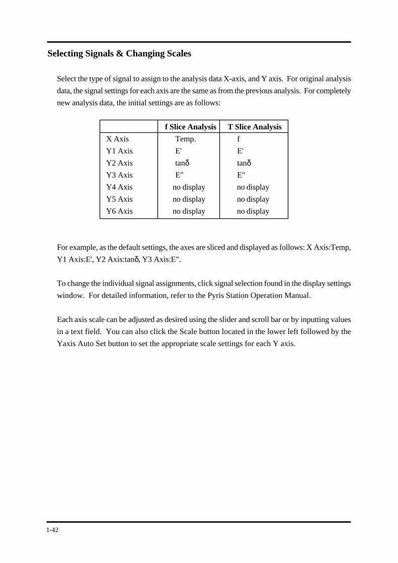
Selecting Signals & Changing Scales
Select the type of signal to assign to the analysis data X-axis, and Y axis. For original analysis
data, the signal settings for each axis are the same as from the previous analysis. For completely
new analysis data, the initial settings are as follows:
f Slice Analysis T Slice Analysis
X Axis Temp. f
Y1 Axis E' E'
Y2 Axis tanδ tanδ Y3 Axis E" E"
Y4 Axis no display no display
Y5 Axis no display no display
Y6 Axis no display no display
For example, as the default settings, the axes are sliced and displayed as follows: X Axis:Temp,
Y1 Axis:E', Y2 Axis:tanδ, Y3 Axis:E".
To change the individual signal assignments, click signal selection found in the display settings
window. For detailed information, refer to the Pyris Station Operation Manual.
Each axis scale can be adjusted as desired using the slider and scroll bar or by inputting values
in a text field. You can also click the Scale button located in the lower left followed by the
Yaxis Auto Set button to set the appropriate scale settings for each Y axis.
1-43
Chapter 1 DMA Measurement & Analysis
NOTE
Read
Reading tanδ peak temperature
1. Click the Read icon.
2. Click the data select button in the Read window and select Y2(tanD).
3. While holding down mouse button 1 (left button), drag the mouse and move the cross
cursor over the tanδ data. When the pointer cursor approaches the peak of the tanδ data,
the cross cursor moves to the peak position of the tanδ data. Release mouse button 1 (left
button) at this point. The cross cursor position determines the indicated point.
4. The temperature, frequency, and tanδ value at the cross cursor point is displayed on the
window and over the data.
When you want to cancel the selected point for any reason, hold down
mouse button 3 in the data area and drag down the edit menu to delete
and release.
5. To read a different frequency peak (example: to select the 1Hz slice), display 1Hz by using
the slider alongside the read window slice selection window.
6. Next, click 1Hz once. The cross cursor on the data moves over the 1Hz tanδ data. Then
perform the operations in steps 3 and 4 again.
7. Click the OK button to close the window.
1-44
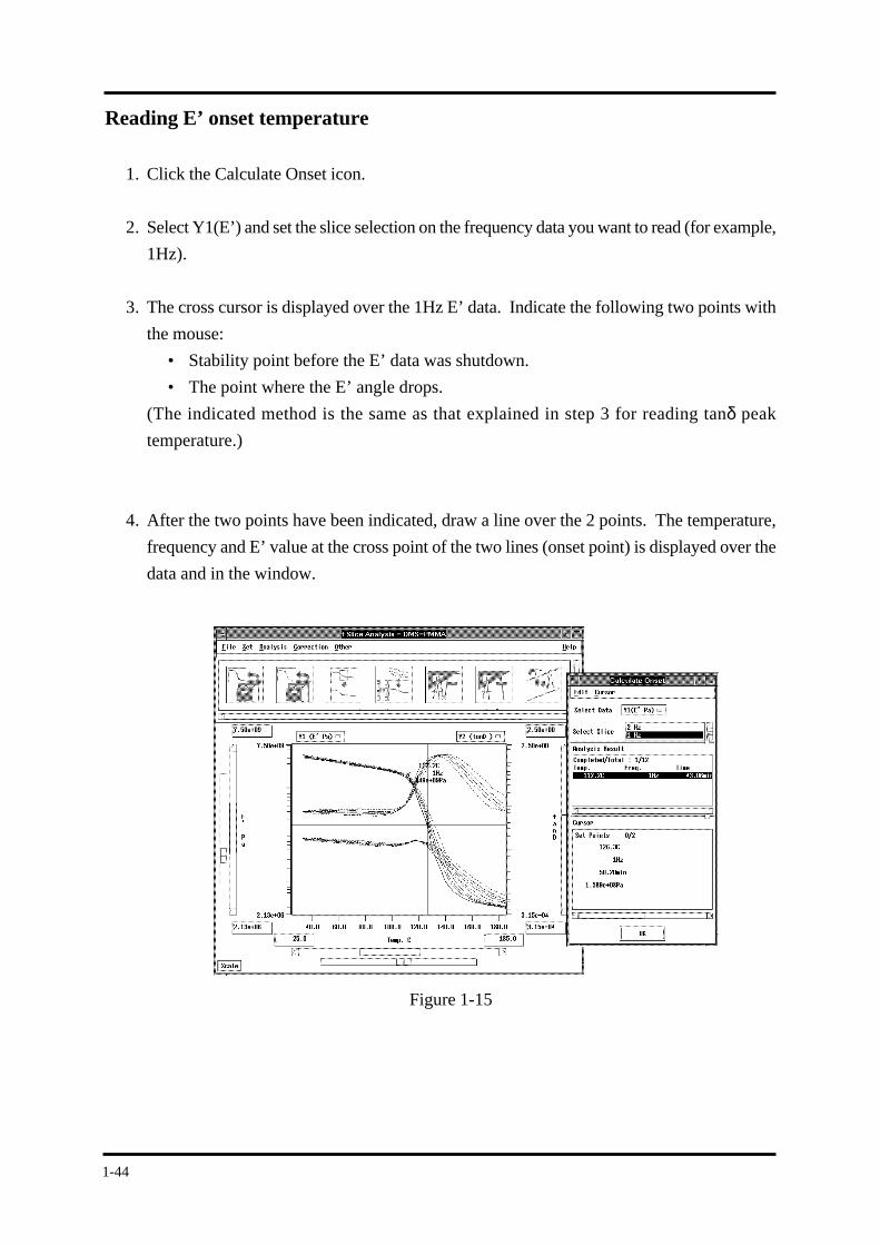
Reading E’ onset temperature
1. Click the Calculate Onset icon.
2. Select Y1(E’) and set the slice selection on the frequency data you want to read (for example,
1Hz).
3. The cross cursor is displayed over the 1Hz E’ data. Indicate the following two points with
the mouse:
• Stability point before the E’ data was shutdown.
• The point where the E’ angle drops.
(The indicated method is the same as that explained in step 3 for reading tanδ peak
temperature.)
4. After the two points have been indicated, draw a line over the 2 points. The temperature,
frequency and E’ value at the cross point of the two lines (onset point) is displayed over the
data and in the window.
Figure 1-15
1-45
Chapter 1 DMA Measurement & Analysis
Editing Analysis Data
Occasionally you may find it necessary to move data numerical displays or edit a data point.
For whatever reason, you can use the following methods to create the most suitable data
points for your measurement needs:
Changing Data Character String Positions
1. Click on one of the four data analysis icons (these icons display a calculator and compass)
to display an analysis window. To select a data point, click on one of the data points listed
in the Analysis Result area.
2. Hold down mouse button #3 (right button) and the Edit menu will appear. Drag the mouse
down to Move Character String and release the mouse button. A single item sub menu will
appear. Click on the single item sub menu with the mouse.
3. A square frame will appear on the data point on the line graph. Click mouse button #1 (left
button) on the frame and move the character string to the desired location.
Editing Data Points in the Calculate Onset Window
1. Click on one of the four data analysis icons (these icons display a calculator and compass)
to display an analysis window. To select a data point, click on one of the data points listed
in the Analysis Result area.
2. Hold down mouse button #3 (right button) and the Edit menu will appear. Drag the mouse
down to Adjust Results and release the mouse button. A sub menu will appear. Align the
mouse on the sub menu and click mouse button #1 (left button).
3. A cross cursor will appear on the data point on the line graph. Click mouse button #1 (left
button) on the center of the cross cursor and move the data point to the desired location.
1-46
NOTE
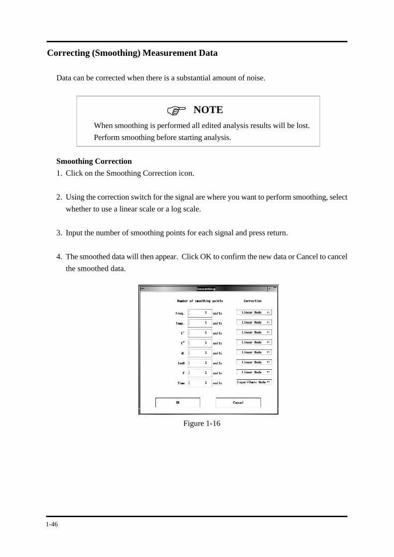
Correcting (Smoothing) Measurement Data
Data can be corrected when there is a substantial amount of noise.
When smoothing is performed all edited analysis results will be lost.
Perform smoothing before starting analysis.
Smoothing Correction
1. Click on the Smoothing Correction icon.
2. Using the correction switch for the signal are where you want to perform smoothing, select
whether to use a linear scale or a log scale.
3. Input the number of smoothing points for each signal and press return.
4. The smoothed data will then appear. Click OK to confirm the new data or Cancel to cancel
the smoothed data.
Figure 1-16
1-47
Chapter 1 DMA Measurement & Analysis
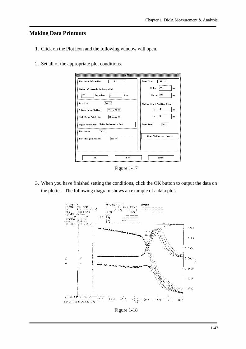
Making Data Printouts
1. Click on the Plot icon and the following window will open.
2. Set all of the appropriate plot conditions.
Figure 1-17
3. When you have finished setting the conditions, click the OK button to output the data on
the plotter. The following diagram shows an example of a data plot.
Figure 1-18
1-48
NOTE
Saving Data
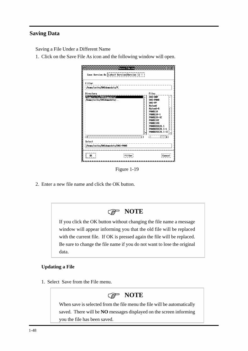
Saving a File Under a Different Name
1. Click on the Save File As icon and the following window will open.
Figure 1-19
2. Enter a new file name and click the OK button.
If you click the OK button without changing the file name a message
window will appear informing you that the old file will be replaced
with the current file. If OK is pressed again the file will be replaced.
Be sure to change the file name if you do not want to lose the original
data.
Updating a File
1. Select Save from the File menu.
When save is selected from the file menu the file will be automatically
saved. There will be NO messages displayed on the screen informing
you the file has been saved.
NOTE
1-49
Chapter 1 DMA Measurement & Analysis
Helpful hints . . .
Changing the X-axis to temperature units
1. Click on the the Display Settings icon.
2. Select X(Time min) from the Select Signal menu.
3. Select Temp. C from the Select Signal area and click the OK button.
4. Click the Display Settings window OK button.
5. A message box will appear asking if it is OK to redisplay the data. Click the OK button.
6. The data will convert to X-axis temperature data.
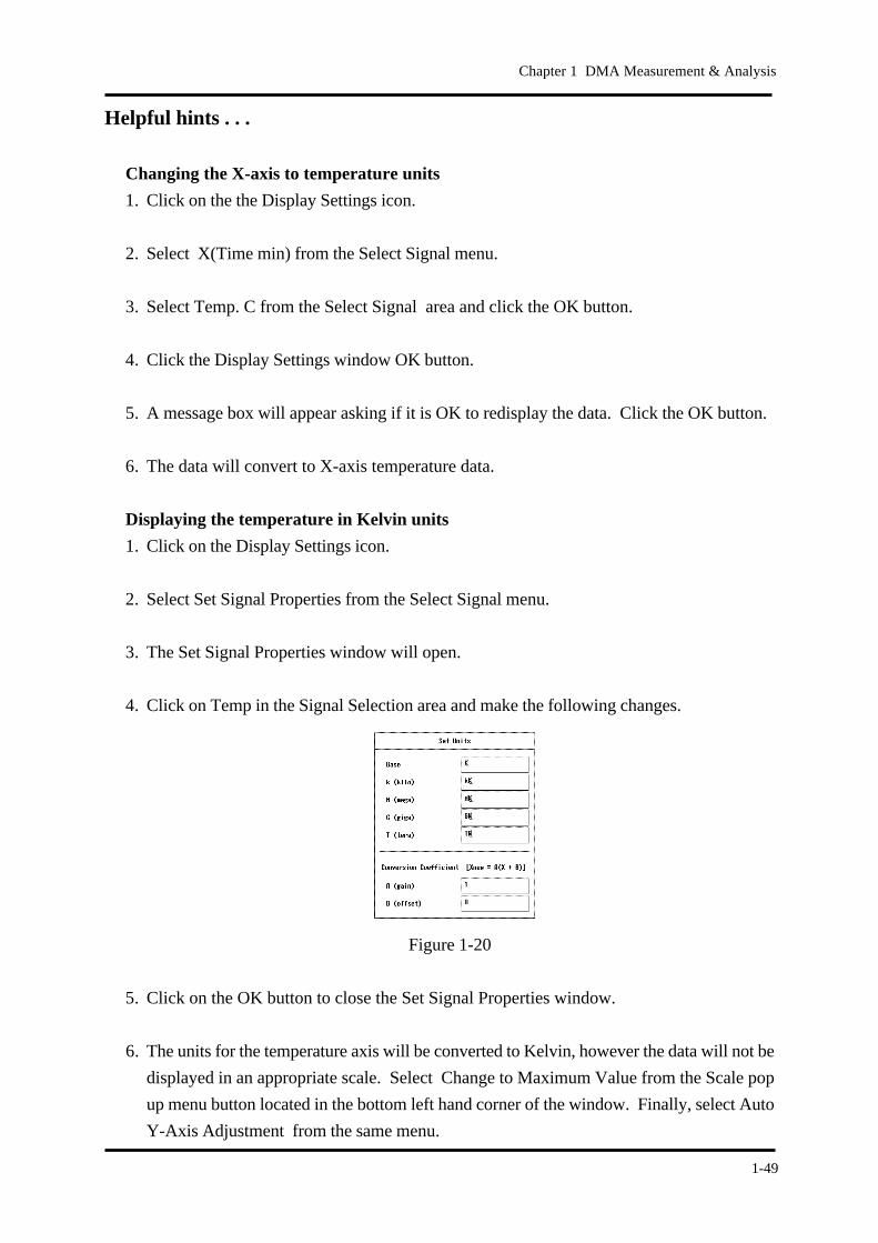
Displaying the temperature in Kelvin units
1. Click on the Display Settings icon.
2. Select Set Signal Properties from the Select Signal menu.
3. The Set Signal Properties window will open.
4. Click on Temp in the Signal Selection area and make the following changes.
Figure 1-20
5. Click on the OK button to close the Set Signal Properties window.
6. The units for the temperature axis will be converted to Kelvin, however the data will not be
displayed in an appropriate scale. Select Change to Maximum Value from the Scale pop
up menu button located in the bottom left hand corner of the window. Finally, select Auto
Y-Axis Adjustment from the same menu.
1-50
Cancelling the Display of Only Specific Slices and Signals
1. Cancelling the display of only specific slices
a. Open the Display Settings window.
b. Double click the slice you do not want to display.
c. The Change Slice Display Properties window appears. Turn OFF the switch of the
particular Yaxis (for example, Y1 • ` Y3).
d. Click the OK button. Click the OK button on the display settings window.
e. A message window is displayed. Click the OK button.
2. Cancelling the display of only specific signals
a. Open the Display Settings window.
b. Click Display Properties from the command menu.
c. To erase the display of only the Y2axis (tanD), click Y2 Axis for All Slices and click
Hide.
d. Click the OK button. Click the OK button on the display settings window.
e. A message window is displayed. Click the OK button.
1-51
Chapter 1 DMA Measurement & Analysis
NOTE
1.6 Analyzing Measurement Data (F, L Control Modes)
Data measured using the DMA Module L Control or F Control modes are saved as TMA data.
Use the TMA/SS Standard Analysis Software to perform analysis of the data.
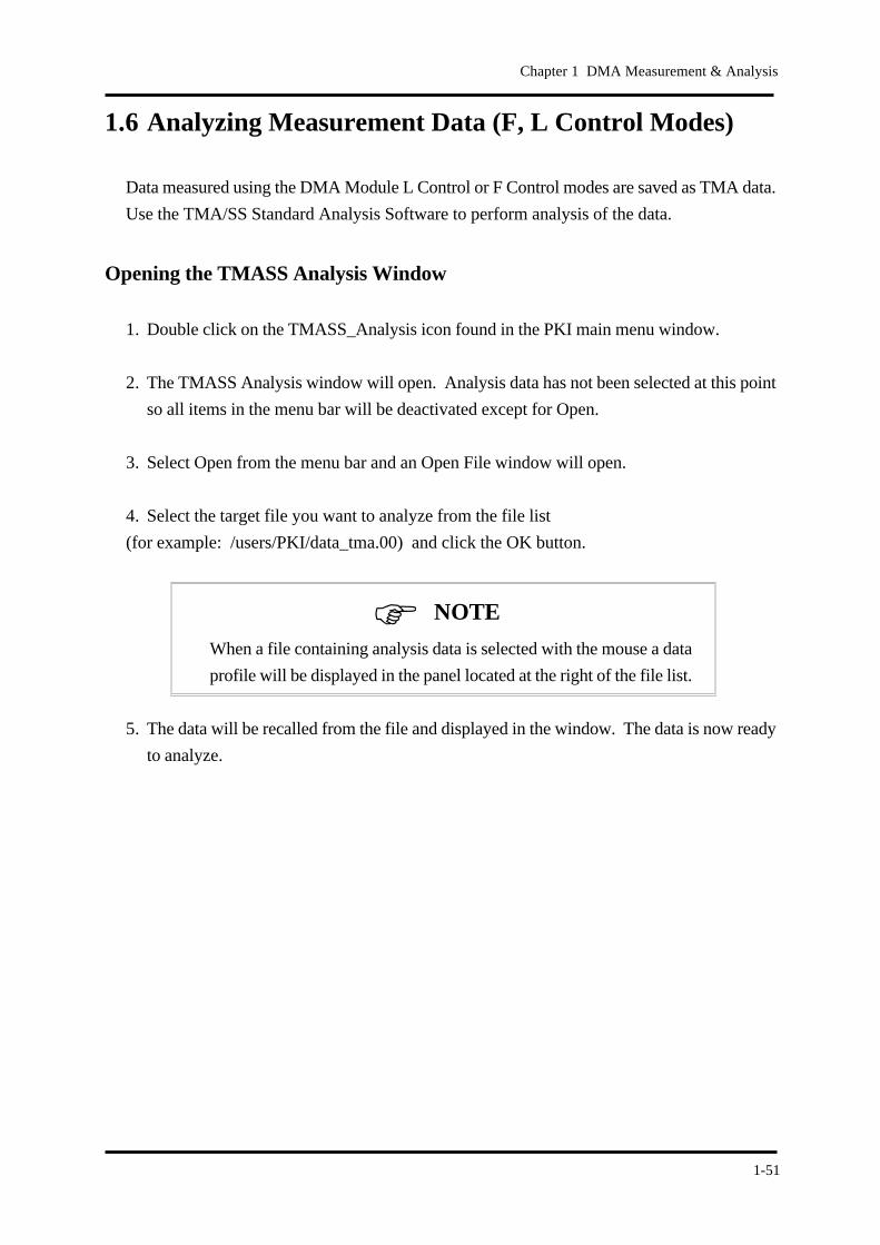
Opening the TMASS Analysis Window
1. Double click on the TMASS_Analysis icon found in the PKI main menu window.
2. The TMASS Analysis window will open. Analysis data has not been selected at this point
so all items in the menu bar will be deactivated except for Open.
3. Select Open from the menu bar and an Open File window will open.
4. Select the target file you want to analyze from the file list
(for example: /users/PKI/data_tma.00) and click the OK button.
When a file containing analysis data is selected with the mouse a data
profile will be displayed in the panel located at the right of the file list.
5. The data will be recalled from the file and displayed in the window. The data is now ready
to analyze.
1-52
Read Point
1. Click the Read Point icon.
2. Select the desired signal in Select Data.
3. Read the signal using one of the following methods:
a. Drag the cross-line cursor on the graph data to the desired position.
b. Use the Cursor pull-down menu in the Read Point window or the click mouse button #3
with the cursor in the graph data and select the cursor movement method. Move the
cursor to the desired location and click Set Point(s) in the same menu.
For an explanation of other types of analysis, refer to the Pyris Thermal Analysis & Rheology
Operation Manual.
1-53
Chapter 1 DMA Measurement & Analysis
Editing Analysis Data
Occasionally you may find it necessary to move data numerical displays or edit a data point.
For whatever reason, you can use the following methods to create the most suitable data
points for your measurement needs:
Changing Data Character String Positions
1. Click on one of the four data analysis icons (these icons display a calculator and compass)
to display an analysis window. To select a data point, click on one of the data points listed
in the Analysis Result area.
2. Hold down mouse button #3 (right button) and the Edit menu will appear. Drag the mouse
down to Move Character String and release the mouse button. A single item sub menu will
appear. Click on the single item sub menu with the mouse.
3. A square frame will appear on the data point on the line graph. Click mouse button #1 (left
button) on the frame and move the character string to the desired location.
1-54
NOTE
Other Corrections
Analysis results are erased once data correction is performed. Be
sure to perform data correction before performing analysis.
Smoothing Correction
1. Click on the Smoothing icon.
2. Input the number of smoothing points for each signal.
3. Click on OK to smooth the data.
Length Normalization
1. Click on the Normalization icon. Their are two types of Normalization items: length and
weight.
2. Enter the Normalize Weight or Normalize Length into the corresponding field.
3. The scale value will change and the peak size will change according to the normalization
correction. Click on OK to confirm or Cancel to cancel this procedure.
1-55
Chapter 1 DMA Measurement & Analysis
NOTE
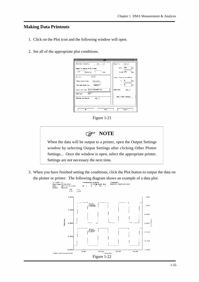
Making Data Printouts
1. Click on the Plot icon and the following window will open.
2. Set all of the appropriate plot conditions.
Figure 1-21
When the data will be output to a printer, open the Output Settings
window by selecting Output Settings after clicking Other Plotter
Settings... Once the window is open, select the appropriate printer.
Settings are not necessary the next time.
3. When you have finished setting the conditions, click the Plot button to output the data on
the plotter or printer. The following diagram shows an example of a data plot.
Figure 1-22
1-56
NOTE
NOTE
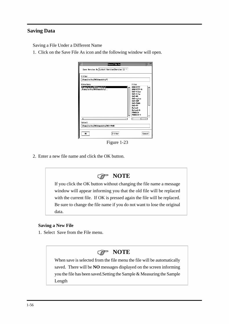
Saving Data
Saving a File Under a Different Name
1. Click on the Save File As icon and the following window will open.
Figure 1-23
2. Enter a new file name and click the OK button.
If you click the OK button without changing the file name a message
window will appear informing you that the old file will be replaced
with the current file. If OK is pressed again the file will be replaced.
Be sure to change the file name if you do not want to lose the original
data.
Saving a New File
1. Select Save from the File menu.
When save is selected from the file menu the file will be automatically
saved. There will be NO messages displayed on the screen informing
you the file has been saved.Setting the Sample & Measuring the Sample
Length
1-57
Chapter 1 DMA Measurement & Analysis
Ending Measurements and Analysis
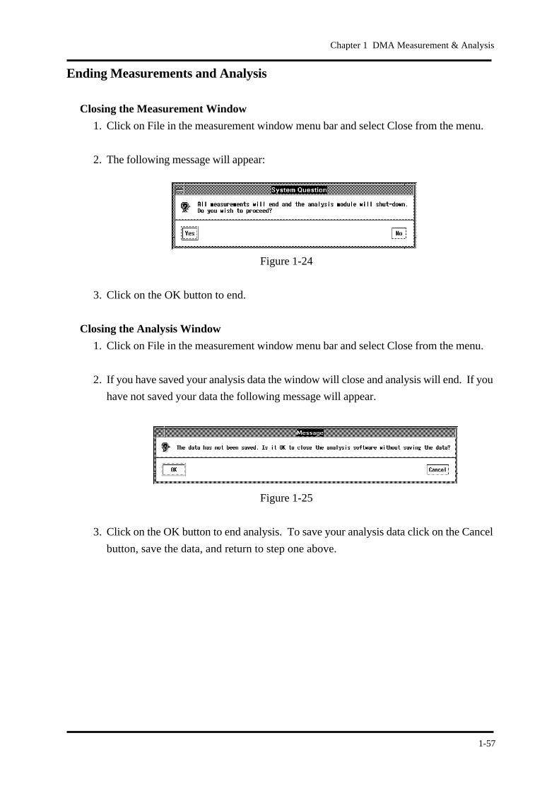
Closing the Measurement Window
1. Click on File in the measurement window menu bar and select Close from the menu.
2. The following message will appear:
Figure 1-24
3. Click on the OK button to end.
Closing the Analysis Window
1. Click on File in the measurement window menu bar and select Close from the menu.
2. If you have saved your analysis data the window will close and analysis will end. If you
have not saved your data the following message will appear.
Figure 1-25
3. Click on the OK button to end analysis. To save your analysis data click on the Cancel
button, save the data, and return to step one above.

1-58
2-1
Chapter 2 DMA Advanced Software Features
Chapter 2 DMA Advanced
Software Features
• Automatic Cooling Feature 2-2
• Protect Feature 2-4
• Temperature Precalibration Feature 2-5
2-2
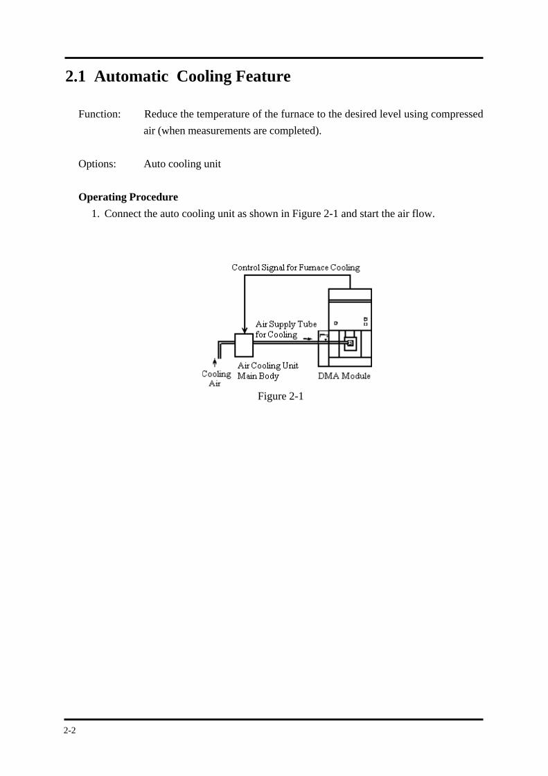
2.1 Automatic Cooling Feature
Function: Reduce the temperature of the furnace to the desired level using compressed
air (when measurements are completed).
Options: Auto cooling unit
Operating Procedure
1. Connect the auto cooling unit as shown in Figure 2-1 and start the air flow.
Figure 2-1
2-3
Chapter 2 DMA Advanced Software Features
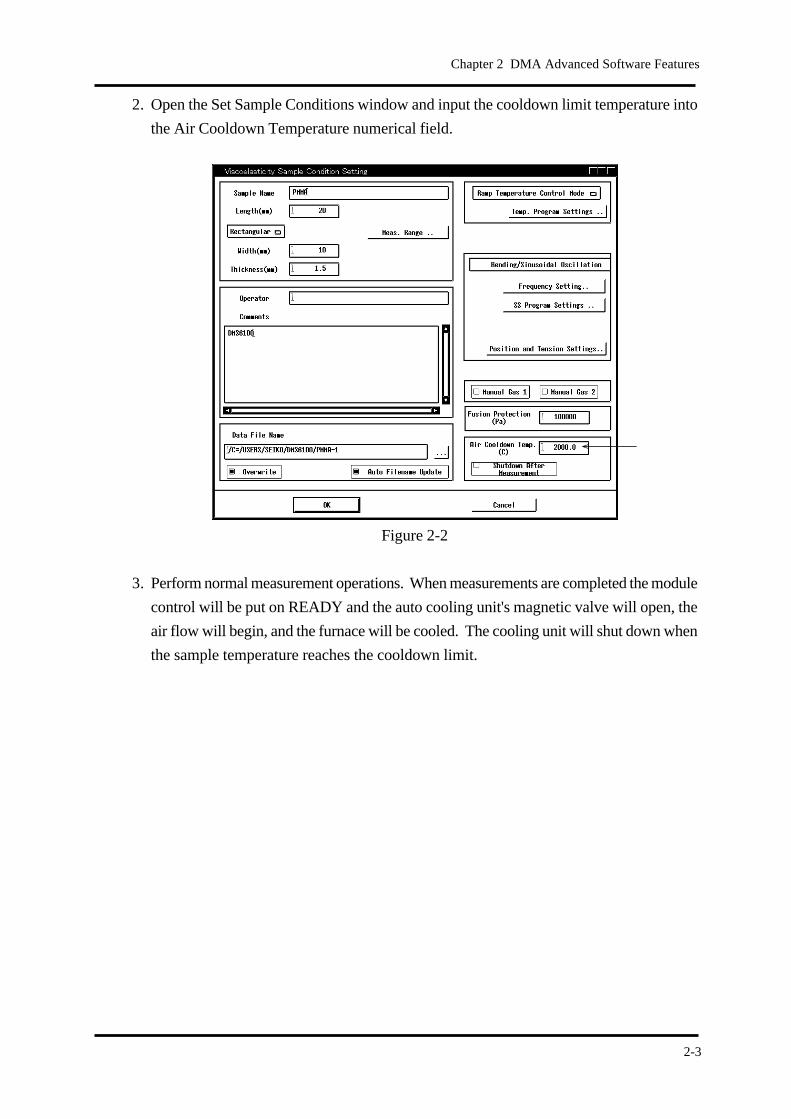
2. Open the Set Sample Conditions window and input the cooldown limit temperature into
the Air Cooldown Temperature numerical field.
Figure 2-2
3. Perform normal measurement operations. When measurements are completed the module
control will be put on READY and the auto cooling unit's magnetic valve will open, the
air flow will begin, and the furnace will be cooled. The cooling unit will shut down when
the sample temperature reaches the cooldown limit.
2-4
2.2 Protect Feature
Function: Prevent sample meltdown on the measuring head or probe.
Module: DMA module
Options: None
Operating Procedure
Operating Procedure
1. Click on the Set Sample Conditions icon.
2. Input a numerical (Pa) value for a E' lower limit value into the Fusion Protection numerical
input field.
Activating the Protect Feature
1. When the E' value is lower than the set value during measurement, the sample is determined
to be softened and the measurement is forceably stopped.
2-5
Chapter 2 DMA Advanced Software Features
2.3 Temperature Precalibration Feature
Function: Keep the difference between the program temperature and sample temperature
at a minimum during measurement. This feature studies the relationship between
both temperatures and corrects and controls the program temperature based
on this relationship.
It is normally not necessary to use this feature when operating a DMA module.
Module: All modules
Options: None
Operating Procedure
Temperature calibration
1. Click on the Set Sample Conditions icon.
2. Click on the Temperature Control Mode pop-up button and select Precalibrated
Temperature Control Mode.
3. Click on the Temperature Program Settings button to display the temperature program
window.
4. Set the following temperature program.
(The following temperature program is an example of a temperature program with a
temperature range from above room temperature to 300°C)
Example of a Temperature Program
End step = 9
Step Start Limit Rate Hold
1 30 60 2 0
2 60 90 2 0
3 90 120 2 0
4 120 150 2 0
5 150 180 2 0
6 180 210 2 0
7 210 240 2 0
8 240 270 2 0
9 270 300 2 0
2-6
1. When the temperature precalibration feature is performed, the loss of
temperature control may be immense for the temperature range outside
of the the temperature precalibration.
2. When performing minus temperature range measurements, set the
temperature program for the minus temperature.
3. An isothermal program with 7 steps or more is necessary. If the
program does not have 7 steps, the precailbration results are not
recorded.
4. A TEST cannot be performed during the Precalibration Temperature
Control mode.
5. Perform measurements.
NOTE
2-7
Chapter 2 DMA Advanced Software Features
NOTE
Measuring after calibration
1. Open the Sample Conditions setting window. Click on the Temperature Control Mode
pop-up menu and select Normal Temperature Control mode. The temperature will
now be controlled based on the precalibrated temperature.
1. Make sure that the control mode is returned to Normal Temperature
Control after the precalibration measurement is performed. If the
temperature control mode is left on Precalibrated Control the
calibration will not be activated and the results will be inaccurate. In
other words, the precalibrated mode will remain "ON" when
measurements are repeated.
2. If temperature precalibration is not performed correctly, the
temperature control of the measurement following the precalibration
is improper and the temperature program does not heat and cool as
set. When this occurs, either perform precalibration again appropriately
or use the following method clear the precalibration results using the
following method and perform the measurement.
a. Click DMS ABC setting icon, and save the necessary ABC
settings in a file.
b. Remove the back-up batteries and turn off the power to the
module.
c. Insert the battery and connect the module to the station.
d. Enter the ABC settings from the file saved in step a.
3. When samples are to be measured under gas flows, set the precalibrated
temperature conditions to match the actual sample measurement
conditions in order to reduce errors. The temperature program data
save feature can be set to either On or Off.

2-8
3-1
Chapter 3 System Calibration
Chapter 3 System Calibration
• PID Temperature Control Constants 3-4
• Sample Temperature Correction 3-5
• Dynamic Viscoelastic Measurement Calibration 3-9
• Static Measurement Mode Load (F)
Sensitivity Correction 3-20
• Adjusting the Strain Signal Output
(Internal Micrometer Adjustment) 3-22
3-2
The DMS ABC Setting window is used to set the constants used for system calibration and
control. We advise that you calibrate your system on a regular basis to maintain peak
performance of your equipment.
The following calibrations are performed from the DMS ABC Setting window:
1. Temperature Control PID Constants Settings
The following three constants are settings for the furnace temperature control:
P=Proportional constant
I=Integral constant
D=Derivative constant
2. Sample Temperature Calibration
Compares the sample temperature with a known (literature) sample temperature and corrects
the offset.
3. Viscoelastic Measurement System Calibration
Correction of the compliance, the inertia of probe mass, the viscoelasticity of the probe
supporting system. Calibration of the elastic modulus from a measurement of a sample
known elastic modulus.
3-3
Chapter 3 System Calibration
NOTE
NOTE
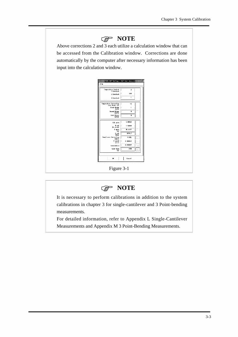
Above corrections 2 and 3 each utilize a calculation window that can
be accessed from the Calibration window. Corrections are done
automatically by the computer after necessary information has been
input into the calculation window.
Figure 3-1
It is necessary to perform calibrations in addition to the system
calibrations in chapter 3 for single-cantilever and 3 Point-bending
measurements.
For detailed information, refer to Appendix L Single-Cantilever
Measurements and Appendix M 3 Point-Bending Measurements.
3-4
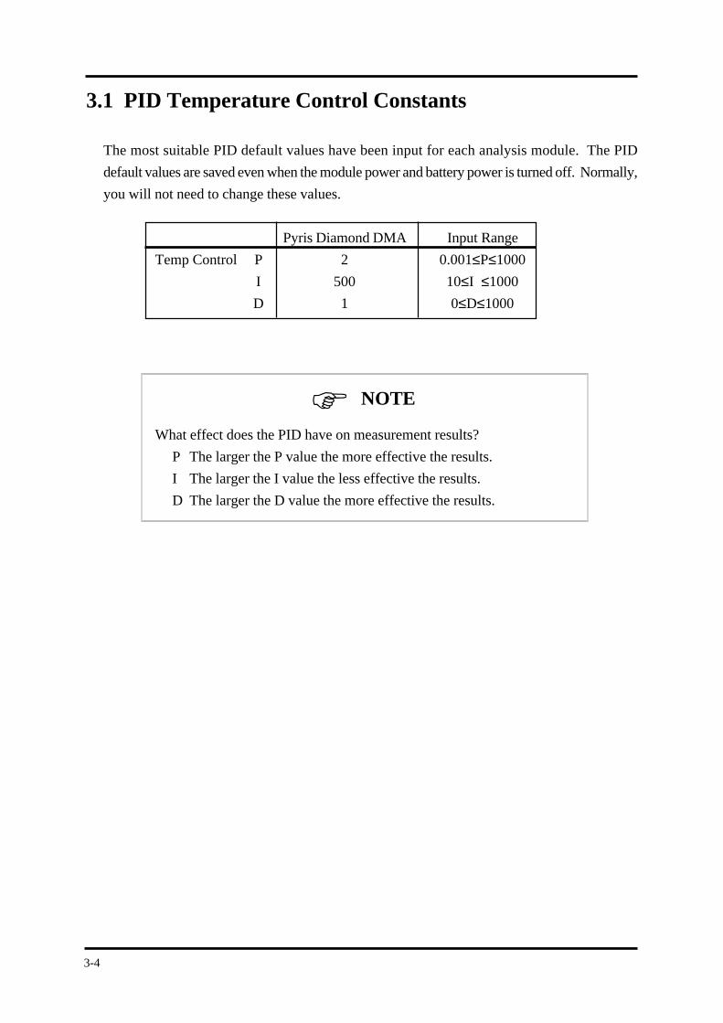
3.1 PID Temperature Control Constants
The most suitable PID default values have been input for each analysis module. The PID
default values are saved even when the module power and battery power is turned off. Normally,
you will not need to change these values.
Pyris Diamond DMA Input Range
Temp Control P 2 0.001≤P≤1000
I 500 10≤I ≤1000
D 1 0≤D≤1000
What effect does the PID have on measurement results?
P The larger the P value the more effective the results.
I The larger the I value the less effective the results.
D The larger the D value the more effective the results.
NOTE
3-5
Chapter 3 System Calibration
NOTE
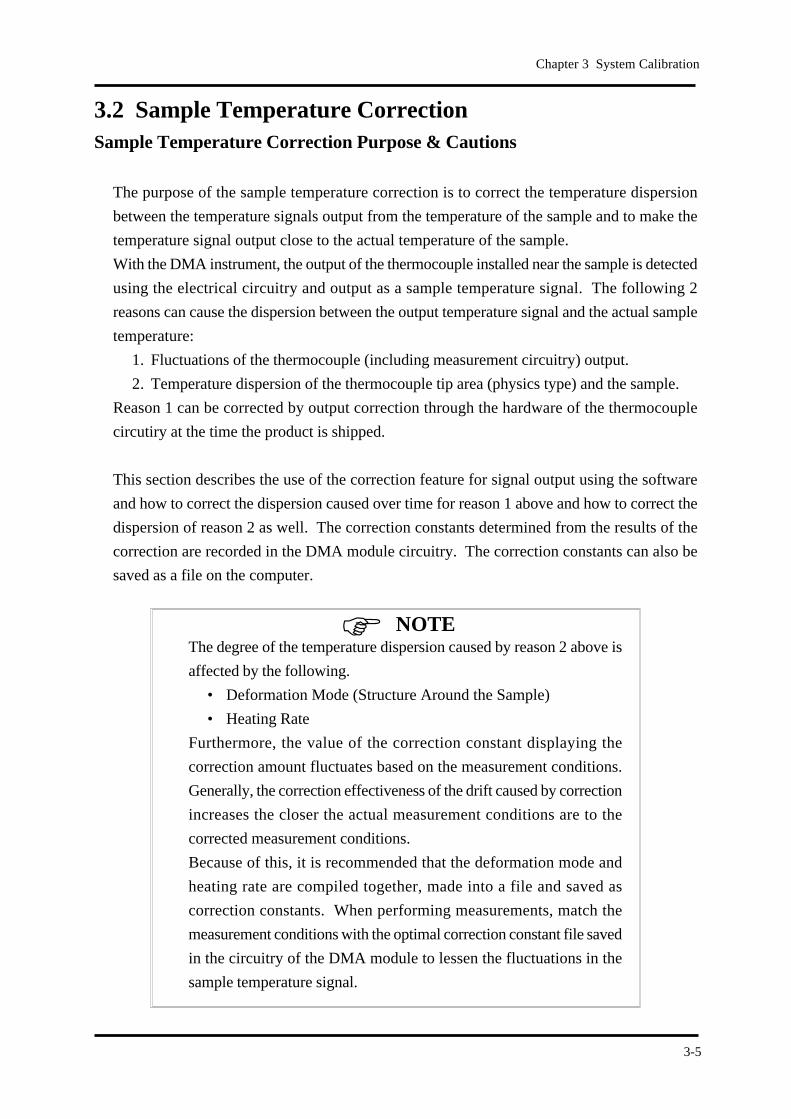
3.2 Sample Temperature CorrectionSample Temperature Correction Purpose & Cautions
The purpose of the sample temperature correction is to correct the temperature dispersion
between the temperature signals output from the temperature of the sample and to make the
temperature signal output close to the actual temperature of the sample.
With the DMA instrument, the output of the thermocouple installed near the sample is detected
using the electrical circuitry and output as a sample temperature signal. The following 2
reasons can cause the dispersion between the output temperature signal and the actual sample
temperature:
1. Fluctuations of the thermocouple (including measurement circuitry) output.
2. Temperature dispersion of the thermocouple tip area (physics type) and the sample.
Reason 1 can be corrected by output correction through the hardware of the thermocouple
circutiry at the time the product is shipped.
This section describes the use of the correction feature for signal output using the software
and how to correct the dispersion caused over time for reason 1 above and how to correct the
dispersion of reason 2 as well. The correction constants determined from the results of the
correction are recorded in the DMA module circuitry. The correction constants can also be
saved as a file on the computer.
The degree of the temperature dispersion caused by reason 2 above is
affected by the following.
• Deformation Mode (Structure Around the Sample)
• Heating Rate
Furthermore, the value of the correction constant displaying the
correction amount fluctuates based on the measurement conditions.
Generally, the correction effectiveness of the drift caused by correction
increases the closer the actual measurement conditions are to the
corrected measurement conditions.
Because of this, it is recommended that the deformation mode and
heating rate are compiled together, made into a file and saved as
correction constants. When performing measurements, match the
measurement conditions with the optimal correction constant file saved
in the circuitry of the DMA module to lessen the fluctuations in the
sample temperature signal.
3-6
In the correction steps, first measure the transition temperature of standard sample, and set the
transition temperature on the literature value. The following is an explanation of correction
using 2°C/min conditions for a tension measurement and 2°C/min conditions for a bending
measurement. When the measurement conditions vary from this, align with the measurement
conditions and perform a correction measurement and create a correction constant file to use.
When the instrument is shipped, sample temperature correction has been performed using a
tension measurement with a 2°C/min condition.
3-7
Chapter 3 System Calibration
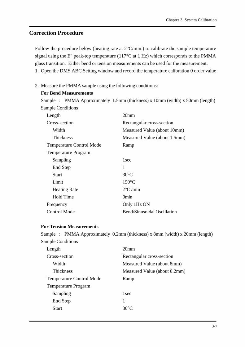
Correction Procedure
Follow the procedure below (heating rate at 2°C/min.) to calibrate the sample temperature
signal using the E" peak-top temperature (117°C at 1 Hz) which corresponds to the PMMA
glass transition. Either bend or tension measurements can be used for the measurement.
1. Open the DMS ABC Setting window and record the temperature calibration 0 order value
2. Measure the PMMA sample using the following conditions:
For Bend Measurements
Sample : PMMA Approximately 1.5mm (thickness) x 10mm (width) x 50mm (length)
Sample Conditions
Length 20mm
Cross-section Rectangular cross-section
Width Measured Value (about 10mm)
Thickness Measured Value (about 1.5mm)
Temperature Control Mode Ramp
Temperature Program
Sampling 1sec
End Step 1
Start 30°C
Limit 150°C
Heating Rate 2°C /min
Hold Time 0min
Frequency Only 1Hz ON
Control Mode Bend/Sinusoidal Oscillation
For Tension Measurements
Sample : PMMA Approximately 0.2mm (thickness) x 8mm (width) x 20mm (length)
Sample Conditions
Length 20mm
Cross-section Rectangular cross-section
Width Measured Value (about 8mm)
Thickness Measured Value (about 0.2mm)
Temperature Control Mode Ramp
Temperature Program
Sampling 1sec
End Step 1
Start 30°C
3-8
NOTE
Limit 150°C
Heating Rate 2°C /min
Hold Time 0min
Frequency Only 1Hz ON
Control Mode Tension/Sinusoidal Oscillation
Position and Tension Settings
L. Amp. 10µm
Min. Tension/Compression Force 300mN
Tension/Compression Force gain 1.5
Force Amplitude Initial Value 4000mN
Approved Maximum Deformation 10000µm
Position Movement Wait Time 8.0sec
Creep Wait Time 0.0sec/mN
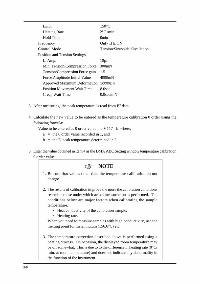
3. After measuring, the peak temperature is read from E" data.
4. Calculate the new value to be entered as the temperature calibration 0 order using the
following formula:
Value to be entered as 0 order value = a + 117 - b where,
a = the 0 order value recorded in 1, and
b = the E' peak temperature determined in 3.
5. Enter the value obtained in item 4 as the DMA ABC Setting window temperature calibration
0 order value.
1. Be sure that values other than the temperature calibration do notchange.
2. The results of calibration improve the more the calibration conditionsresemble those under which actual measurement is performed. Theconditions below are major factors when calibrating the sampletemperature.
• Heat conductivity of the calibration sample.• Heating rate.
When you need to measure samples with high conductivity, use themelting point for metal indium (156.6°C) etc..
3. The temperature correction described above is performed using aheating process. On occasion, the displayed room temperature maybe off somewhat. This is due to to the difference in heating rate (0°C/min. at room temperature) and does not indicate any abnormality inthe function of the instrument.
3-9
Chapter 3 System Calibration
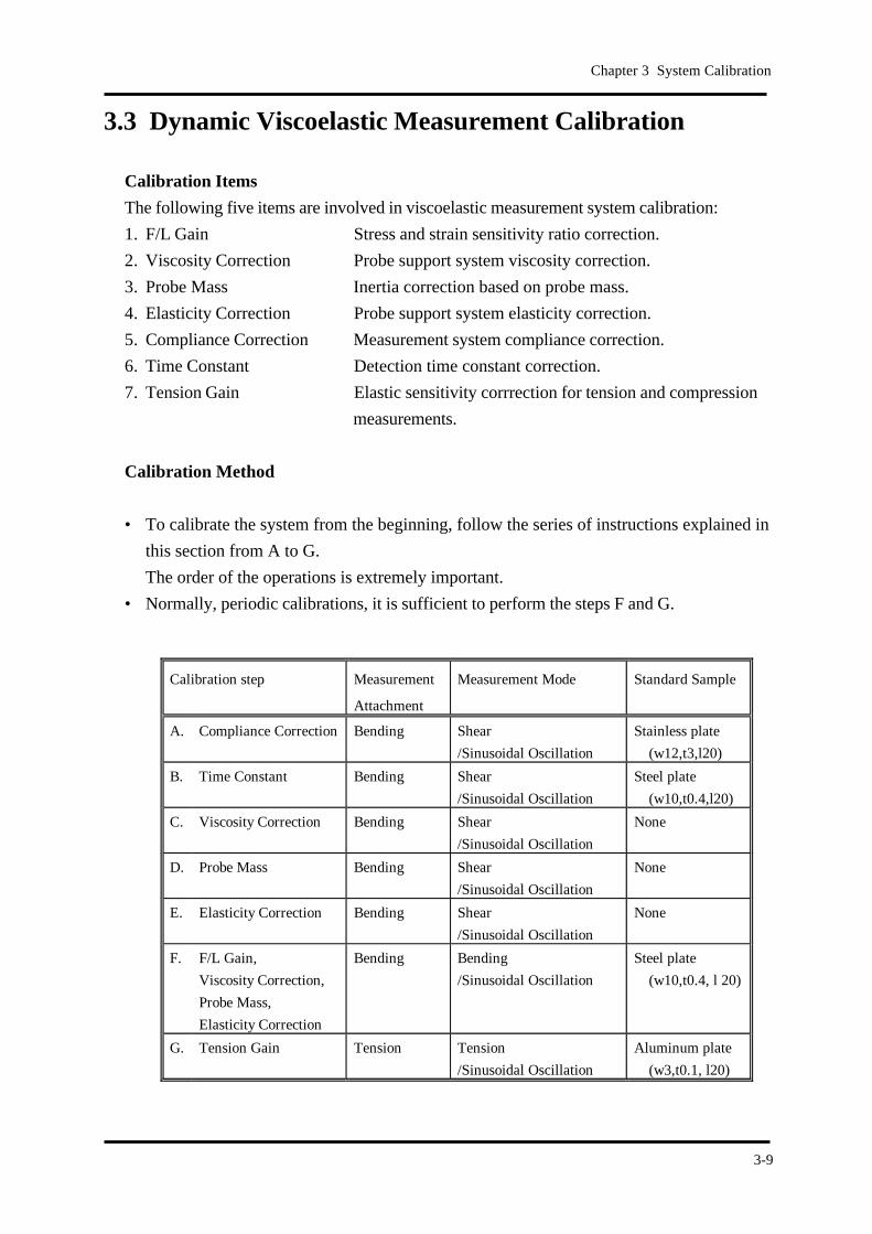
3.3 Dynamic Viscoelastic Measurement Calibration
Calibration Items
The following five items are involved in viscoelastic measurement system calibration:
1. F/L Gain Stress and strain sensitivity ratio correction.
2. Viscosity Correction Probe support system viscosity correction.
3. Probe Mass Inertia correction based on probe mass.
4. Elasticity Correction Probe support system elasticity correction.
5. Compliance Correction Measurement system compliance correction.
6. Time Constant Detection time constant correction.
7. Tension Gain Elastic sensitivity corrrection for tension and compression
measurements.
Calibration Method
• To calibrate the system from the beginning, follow the series of instructions explained in
this section from A to G.
The order of the operations is extremely important.
• Normally, periodic calibrations, it is sufficient to perform the steps F and G.
Calibration step Measurement
Attachment
Measurement Mode Standard Sample
A. Compliance Correction Bending Shear
/Sinusoidal Oscillation
Stainless plate
(w12,t3,l20)
B. Time Constant Bending Shear
/Sinusoidal Oscillation
Steel plate
(w10,t0.4,l20)
C. Viscosity Correction Bending Shear
/Sinusoidal Oscillation
None
D. Probe Mass Bending Shear
/Sinusoidal Oscillation
None
E. Elasticity Correction Bending Shear
/Sinusoidal Oscillation
None
F. F/L Gain,
Viscosity Correction,
Probe Mass,
Elasticity Correction
Bending Bending
/Sinusoidal Oscillation
Steel plate
(w10,t0.4, l 20)
G. Tension Gain Tension Tension
/Sinusoidal Oscillation
Aluminum plate
(w3,t0.1, l20)
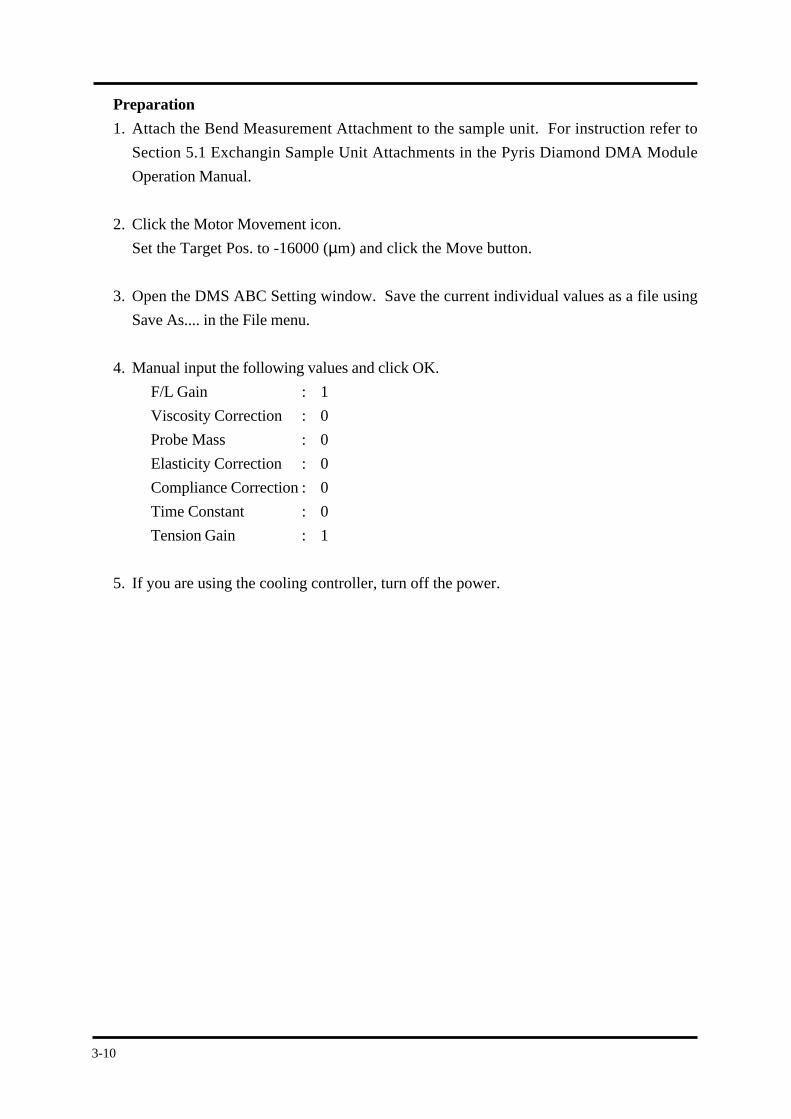
3-10
Preparation
1. Attach the Bend Measurement Attachment to the sample unit. For instruction refer to
Section 5.1 Exchangin Sample Unit Attachments in the Pyris Diamond DMA Module
Operation Manual.
2. Click the Motor Movement icon.
Set the Target Pos. to -16000 (µm) and click the Move button.
3. Open the DMS ABC Setting window. Save the current individual values as a file using
Save As.... in the File menu.
4. Manual input the following values and click OK.
F/L Gain : 1
Viscosity Correction : 0
Probe Mass : 0
Elasticity Correction : 0
Compliance Correction : 0
Time Constant : 0
Tension Gain : 1
5. If you are using the cooling controller, turn off the power.
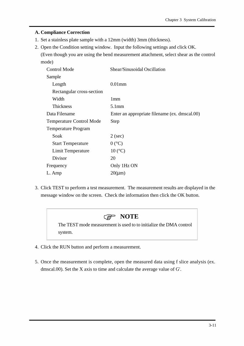
3-11
Chapter 3 System Calibration
NOTE
A. Compliance Correction
1. Set a stainless plate sample with a 12mm (width) 3mm (thickness).
2. Open the Condition setting window. Input the following settings and click OK.
(Even though you are using the bend measurement attachment, select shear as the control
mode)
Control Mode Shear/Sinusoidal Oscillation
Sample
Length 0.01mm
Rectangular cross-section
Width 1mm
Thickness 5.1mm
Data Filename Enter an appropriate filename (ex. dmscal.00)
Temperature Control Mode Step
Temperature Program
Soak 2 (sec)
Start Temperature 0 (°C)
Limit Temperature 10 (°C)
Divisor 20
Frequency Only 1Hz ON
L. Amp 20(µm)
3. Click TEST to perform a test measurement. The measurement results are displayed in the
message window on the screen. Check the information then click the OK button.
The TEST mode measurement is used to to initialize the DMA control
system.
4. Click the RUN button and perform a measurement.
5. Once the measurement is complete, open the measured data using f slice analysis (ex.
dmscal.00). Set the X axis to time and calculate the average value of G'.
3-12
NOTE
NOTEAfter using the f slice analysis Display Settings, Signal Selection and
Signal Properties Setting windows to set the signal selection to G'Pa,
the A (gain) and B (offset) functions in the bottom left of the window
should be 1, 0 respectively. If the values are different, enter A=1 and
B=0 and click the OK. Next, click OK on the Display Settings window.
6. Open the DMS ABC Setting window. Click the Compliance correction calculation button.
Input the elastic modulus value (M') from the message window into the Actual Measured
value E' area in the automatic correction calculation window and click OK.
7. The compliance correction calculated value is input. If the value is correct it will be in the
10-4 ~ 10-3 order. Click OK.
Be sure to click the OK button one time and close the window. If the
window is left open, the correction value will not be activated.
3-13
Chapter 3 System Calibration
NOTE
B. Time Constant
1. Remove the stainless plate and chuck a 10mm width, 0.4mm thickness steel plate.
2. Open the Frquency Settings window, turn on the 100Hz button and click OK.
3. Select display type 2 (time), turn off the tanD Log Display and click the OK button.
4. Click TEST to perform a test measurement. The measurement results are displayed in the
message window on the screen. Check the information then click the OK button.
5. Click Run and begin the measurement. Magnify the tanδ scale and read the tanδ measurement
value.
6. Open the DMS ABC Setting window and click the time constant calculation. Input the
following and click the OK button.
Actual Measured tanD : tanδ read in step 5
Offset : 0.005
Measurement Freq. : 100 (Hz)
7. The calculation results are entered into the time constant. If the calculations is normal, the
calculation value should be in the 10-4 order. Click the OK button.
8. After clicking OK, make sure that the tanδ value of the measured data has dropped to
around 0.005.
9. Click the STOP button and stop the measurement.
If the measurement stops during steps 5 ~ 8, click the RUN button
again.
3-14
NOTE
NOTE
C. Viscosity Correction
1. Open the Frequency Settings window, click ON the 20Hz frequency only and click the OK
button.
2. Remove the steel plate to create a blank status (leave chuck attached).
3. Click the Motor Move icon, enter 10mN for the Force Amplitude Initial Value. Enter
values around 700mN for the Offset Load and adjust the value so that the L (strain signal)
value is within 0.5µm.
1. The Offset Load value is effective when the instrument is first operated
after the value has been entered and the OK button clicked.
2. When the Offset Load is changed by 10mN, the L (strain signal) changes
from -3 to -4µm.
4. Click Test and perform a test measurement. Make sure the elastic modulus value is displayed
in the message panel and click the OK button
5. Click the Run button and enlarge the tanδ scale to 0 ~ 0.4 and read an approximate tanδmeasurement value.
6. Open the DMS ABC Setting window. Enter a value of 0.5 ~ 2 in the V cal area and click
the OK button.
7. Repeat step 6 until the tanδ data is in a range of about 0.002 ~ 0.02.
With the sample absent, the signal is not stable due to tanδ = E"/E' =
0/0. There is no problem with the instrument in this case. Once the
measurements in steps 6 through 7 are completed, click Run again.
3-15
Chapter 3 System Calibration
NOTE
NOTE
D. Probe Mass
1. Click the STOP button and stop the measurement.
2. Click the Frequency Setting icon and turn ON frequency 1Hz, 10Hz, 20Hz. Click the OK
button.
3. Open the Display Setting window, turn ON display type 3 (frequency) and click the OK
button.
Check to make sure the following settings are entered in the Conditions
setting window. After checking the settings, click the OK button.
Length : 0.01(mm)
Rectangular Cross Section
Width : 1 (mm)
Thickness : 5.1 (mm2)
4. Click TEST to perform a test measurement. The measurement results are displayed in the
message window on the screen. Check the information then click the OK button.
5. Click Run and begin the measurement. Magnify the G' scale.
6. Open the DMS ABC Setting window. Enter values of 50 ~ 100 in the P mass and click the
OK button.
7. Change and adjust the probe mass values in step 6 until the E' signal is flat. If the operation
works correctly, the appropriate value should be 50 ~ 100.
If the measurement stops during steps 6 ~ 7, click the RUN button
again.
3-16
NOTE
E. Elasticity Correction
1. Click the STOP button and stop the measurement.
2. Open the measured data using f Slice Analysis and read the 1Hz value of E' (1000 ~3000).
3. Open the DMS ABC Setting window. Enter the value from step 2 into elastic correction
input field and click the OK button.
The measurement value in step 2 is a blank measurement and is
therefore relatively unstable. This is not an abnormality.
3-17
Chapter 3 System Calibration
NOTE
F. F/L Gain, Viscosity Correction, Probe Mass, Elasticity Correction
1. Perform chucking again on a chuck a 10mm width, 0.4mm thickness steel plate.
2. Click the Motor Movement icon, enter 2000mN for the Force Amplitude Initial Value then
click the OK button.
3. Open the Condition setting window. Input the following settings and click OK.
Sample
Length 20mm
Rectangular cross-section
Width 10mm
Thickness 0.4mm
Frequency Only 1Hz ON
Control Mode Bend/Sinusoidal Oscillation
Measure the width and thickness of the stainless board and enter the
actual measured values.
4. Click Test and perform a test measurement. Make sure the elastic modulus value is displayed
in the message panel and click the OK button
5. Click the Run button and perform a measurement.
6. Once the measurement is complete, open the measured data using f slice analysis (ex.
dmscal.00). Set the X axis to time and calculate the average value of E'.
7. Open the DMS ABC Setting window. Click the F/L Gain calculation button.
8. Enter the following values into the Auto Calculation window.
Literature Value E' : 1.92E + 11
Actual Measured E' : The average elasticity (E') value calculated in step 6.
Constant Changes : F/L Gain, Vcal, Pmass and Ecal All ON.
9. Click the OK button in the Auto Calculation window. The F/L Gain, Viscosity Correction,
Probe Mass and Elasticity Correction values are chaned to the calculated results. Click the
OK button.
3-18
NOTE
G. Tension Gain
1. Attach the Tension Measurement Attachment to the sample unit. For instruction refer to
Section 5.1 Exchangin Sample Unit Attachments in the Pyris Diamond DMA Module
Operation Manual.
2. Open the Position Settings/Tension Conditions setting window and click the Initialize button.
Once initialization is complete, click the OK button and close the window.
3. Perform chucking again on a chuck a 3mm width, 0.1mm thickness Alminum sample.
4. Open the Sample Setting window. Input the following settings and click the OK button.
Sample Shape
Length 20 (mm)
Rectangular cross section
Width 3 (mm)
Thickness 0.1 (mm)
Frequency Setting Only 1Hz ON
Control Mode Tension
Position and Tension Settings
Min. Tension/Compression Force 300mN
Tension/Compression Force Gain 1.5
Force Amplitude Initial Value 4000mN
Correctly observe the aluminum sample width and thickness and enter
the actual measured value.
5. Click the TEST button to perform a test measurement. Leave the result message window
open.
6. Click Run and begin the measurement.
7. Once the measurement is completed, open the measurement data using f Slice Analysis.
Set the X axis to time and read the E' value. Calculate an average E' value.
8. Open the DMA ABC Setting window and click the Tension Gain calculation button.
3-19
Chapter 3 System Calibration
NOTE
NOTE
9. Enter the following into the Auto Calculation window:
Literature E' Value : 6.91E + 10
Actual Measured E‘ : The E' average value from step 7.
10.Click the OK button in the Auto Calculation window. The Tension Gain value is
automatically updated (the calculation value becomes 0.8 ~ 1.2).
The Tension Gain value is recalculated and updated each time the OK
button is clicked in the Auto Calculation window. To return to the
previous calculation click the Cancel button.
11.Click the RUN button again and perform a measurement. Make sure that the elasticity of
the aluminum is output correctly. This completes all calibrations.
Normally, for periodic calibrations, it is sufficient to perform the steps
in D. F/L Gain, Viscosity Correction, Probe Mass, Elasticity
Correction with the Bend Measurement Attachment attached and then
perform G. Tension Gain with the Tension Meausrement Attachment
attached. These operations will complete system calibrations.
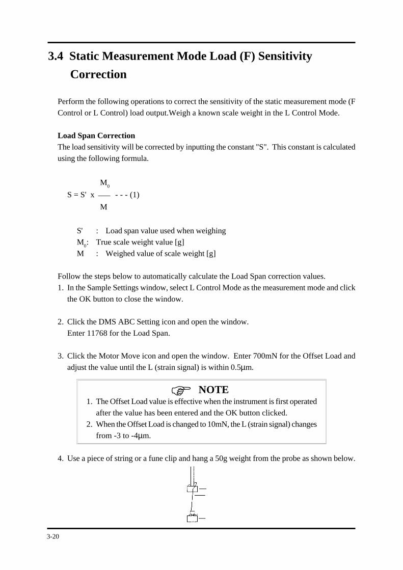
3-20
NOTE
3.4 Static Measurement Mode Load (F) Sensitivity
Correction
Perform the following operations to correct the sensitivity of the static measurement mode (F
Control or L Control) load output.Weigh a known scale weight in the L Control Mode.
Load Span Correction
The load sensitivity will be corrected by inputting the constant "S". This constant is calculated
using the following formula.
M0
S = S' x - - - (1)
M
S' : Load span value used when weighing
M0: True scale weight value [g]
M : Weighed value of scale weight [g]
Follow the steps below to automatically calculate the Load Span correction values.
1. In the Sample Settings window, select L Control Mode as the measurement mode and click
the OK button to close the window.
2. Click the DMS ABC Setting icon and open the window.
Enter 11768 for the Load Span.
3. Click the Motor Move icon and open the window. Enter 700mN for the Offset Load and
adjust the value until the L (strain signal) is within 0.5µm.
1. The Offset Load value is effective when the instrument is first operated
after the value has been entered and the OK button clicked.
2. When the Offset Load is changed to 10mN, the L (strain signal) changes
from -3 to -4µm.
4. Use a piece of string or a fune clip and hang a 50g weight from the probe as shown below.
3-21
Chapter 3 System Calibration
5. Create a program that holds the SS Program at 0µm and holds the temperature program at
0°C.
SS Program Example
End Step : 1
Start Position : 0µm
Limit Position : 0µm
Displacement Rate : 100µm/min (anything is acceptable)
Hold Time : 10min
6. Click the RUN button and begin the measurement.
7. After a short time, the L (strain signal) will stabilize at 0µm. Read the F output value when
this occurs.
8. Open the right Load Span Auto Calculation window in the DMS ABC Settings window.
9. Enter 490.333mN in the Literature Value and for the Actual Value enter the value from
step 6 and click the OK button. The Load Span is automatically calculated and entered.
The gravitation applied to a 50g weight using the standard acceleration
of free fall (9.80665ms-2) computes as follows:
0.05kg × 9.80665ms-2 = 490.333mN.
Information
3-22
NOTE
3.5 Adjusting the Strain Signal Output
(Internal Micrometer Adjustment)
If one of the following occurs, there is probably a problem in the adjustment of the micrometer
within the system.
a. With the sample removed, the strain signal is out of the ±30µm range even though the
offset load value in the Motor Setting window has not been changed to a great extent.
b. With the sample removed, the strain signal value is out of the ±50µm range when 700mN
is entered for the offset load value in the Motor Setting window.
In the following case, even if the symptoms above occur, there is not a
need to adjust the micrometer. First check the items below before
performing adjustments.
1. The sample is attached.
Remove the sample. With only the chuck attached, check the other
items.
2. The battery voltage is low or the batteries have just been replaced.
In this case, check to see if case b above occurs when 700mN is entered
for the Offset Load.
3. When the measurement mode is set to 3 point-bending (sinusoidal or
synthetic oscillation), tension (sinusoidal or synthetic oscillation),
compression (sinusoidal or synthetic oscillation) and a value other
than 0 is entered for the Tension/Compression Minimum Value.
In this case, check to see if case a or b above occurs when the mode is
switched to the single-cantilever mode.
4. The measurement mode is set to the F Control Mode and a value
other than 0 is entered for the 1 Step Start Load in the SS Program.
In this case, check to see if case a or b above occurs when the mode is
switched to the L Control Mode.
3-23
Chapter 3 System Calibration
NOTE
Follow the steps below to perform strain output adjustment using the micrometer.
1. Select the L Control Mode and make sure the system is in the Ready status.
2. Open the front panel.
3. Remove the front plate of the detection system purge box (made of stainless steel).
4. Click the Motor Move icon, enter 700mN for the Offset Load and click the OK button.
5. Adjust the micrometer so that the L (strain signal) is in the ±10µm range.
The micrometer is very sensitive to movements and only requires small
movements for adjustments (1 turn = 1/10). Be careful not to turn the
micrometer a large amount.
When the signal value is over ±200µm, contact Service.
6. After performing adjustments, tighten the screws on the front panel of the detection system
purge box and close the front panel.

3-24
A-1
Appendix A Dynamic Viscoelastic Measurement Range
Appendix A Dynamic Viscoelasticity
Measurement Range
A-2
A-1. Introduction
Whether the dynamic viscoelasticity of a certain sample can be measured depends on the
elastic modulus of the sample, the sample shape and dimensions as well as the deformation
mode (bend, tension, compression, shear) and measurement mode (sinusoidal osciallation mode,
synthetic oscillation mode). A measurement range exists for each value and if the value is out
of the range the measurement cannot be performed or the error of the measurement value is
extremely large.
Furthermore, in order to obtain quality data it is extremely important to correctly confirm that
the value is within the measurement range before performing the measurement. Before
performing the measurement, adjust the sample to the optimum dimensions and select the
appropriate deformation mode and measurement mode.
A-2. Sample Dimension Criterion
For the elasticity modulus of the sample, refer to the literature values and measurement values
when available. When the values are not known, place the sample in the instrument and
perform a test measurement to determine the values.
For the sample dimensions, adjust (bend measurement) the thickness of the sample and make
the cross section area smaller (tension measurement) for hard samples. The opposite should
be performed for soft samples.
As a reference, a representative polymer sample is shown in Table A-1 below. Table A-2
shows the approximate elasticity range of other samples. The optimum sample shape can be
determined from the elasticity modulus range but only the criterion for the sample dimensions
for the bend measurement and tension measurement are shown here.
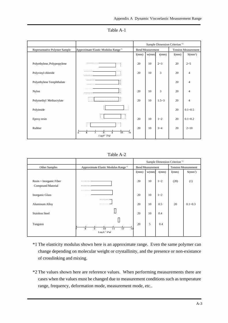
A-3
Appendix A Dynamic Viscoelastic Measurement Range
Table A-1
Sample Dimension Criterion *2
Representative Polymer Sample Approximate Elastic Modulus Range *1 Bend Measurement Tension Measurement
l(mm) w(mm) t(mm) l(mm) S(mm2)
Polyethylene, Polypropylene 20 10 2~3 20 2~5
Polyvinyl chloride 20 10 3 20 4
Polyethylene Terephthalate 20 4
Nylon 20 10 3 20 4
Polymethyl Methacrylate 20 10 1.5~3 20 4
Polyimide 20 0.1~0.5
Epoxy resin 20 10 1~2 20 0.1~0.2
Rubber 20 10 3~4 20 2~10
Table A-2
Sample Dimension Criterion *2
Other Samples Approximate Elastic Modulus Range *1 Bend Measurement Tension Measurement
l(mm) w(mm) t(mm) l(mm) S(mm2)
Resin + Inorganic Fiber 20 10 1~2 (20) (1)
Compound Material
Inorganic Glass 20 10 1~2
Aluminum Alloy 20 10 0.5 20 0.1~0.3
Stainless Steel 20 10 0.4
Tungsten 20 5 0.4
*1 The elasticity modulus shown here is an approximate range. Even the same polymer can
change depending on molecular weight or crystallinity, and the presence or non-existance
of crosslinking and mixing.
*2 The values shown here are reference values. When performing measurements there are
cases when the values must be changed due to measurement conditions such as temperature
range, frequency, deformation mode, measurement mode, etc..
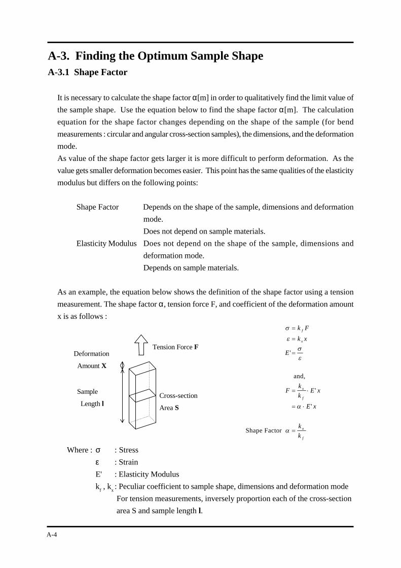
A-4
A-3. Finding the Optimum Sample ShapeA-3.1 Shape Factor
It is necessary to calculate the shape factor α[m] in order to qualitatively find the limit value of
the sample shape. Use the equation below to find the shape factor α[m]. The calculation
equation for the shape factor changes depending on the shape of the sample (for bend
measurements : circular and angular cross-section samples), the dimensions, and the deformation
mode.
As value of the shape factor gets larger it is more difficult to perform deformation. As the
value gets smaller deformation becomes easier. This point has the same qualities of the elasticity
modulus but differs on the following points:
Shape Factor Depends on the shape of the sample, dimensions and deformation
mode.
Does not depend on sample materials.
Elasticity Modulus Does not depend on the shape of the sample, dimensions and
deformation mode.
Depends on sample materials.
As an example, the equation below shows the definition of the shape factor using a tension
measurement. The shape factor α, tension force F, and coefficient of the deformation amount
x is as follows :
Where : σ : Stress
ε : Strain
E' : Elasticity Modulus
kf , k
x: Peculiar coefficient to sample shape, dimensions and deformation mode
For tension measurements, inversely proportion each of the cross-section
area S and sample length l.
Cross-section
Area S
Tension Force F
Sample
Length l
Deformation
Amount X
σ
εσε
α
α
=
=
=
= ⋅
= ⋅
=
k F
k x
E
Fk
kE x
E x
k
k
f
x
x
f
x
f
'
'
'
and,
Shape Factor
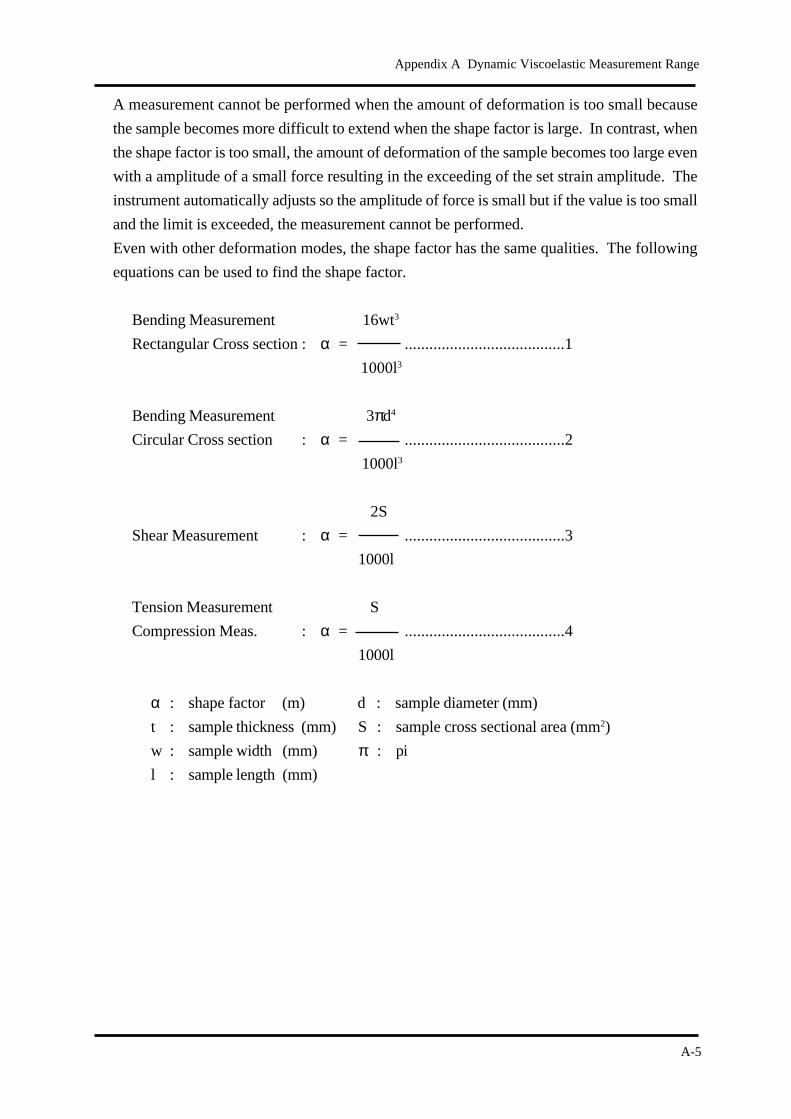
A-5
Appendix A Dynamic Viscoelastic Measurement Range
A measurement cannot be performed when the amount of deformation is too small because
the sample becomes more difficult to extend when the shape factor is large. In contrast, when
the shape factor is too small, the amount of deformation of the sample becomes too large even
with a amplitude of a small force resulting in the exceeding of the set strain amplitude. The
instrument automatically adjusts so the amplitude of force is small but if the value is too small
and the limit is exceeded, the measurement cannot be performed.
Even with other deformation modes, the shape factor has the same qualities. The following
equations can be used to find the shape factor.
Bending Measurement 16wt3
Rectangular Cross section : α = .......................................1
1000l3
Bending Measurement 3πd4
Circular Cross section : α = .......................................2
1000l3
2S
Shear Measurement : α = .......................................3
1000l
Tension Measurement S
Compression Meas. : α = .......................................4
1000l
α : shape factor (m) d : sample diameter (mm)
t : sample thickness (mm) S : sample cross sectional area (mm2)
w : sample width (mm) π : pi
l : sample length (mm)
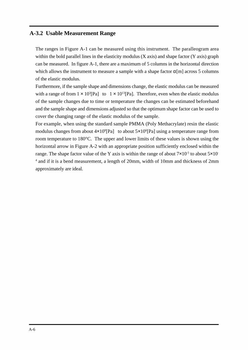
A-6
A-3.2 Usable Measurement Range
The ranges in Figure A-1 can be measured using this instrument. The paralleogram area
within the bold parallel lines in the elasticity modulus (X axis) and shape factor (Y axis) graph
can be measured. In figure A-1, there are a maximum of 5 columns in the horizontal direction
which allows the instrument to measure a sample with a shape factor α[m] across 5 columns
of the elastic modulus.
Furthermore, if the sample shape and dimensions change, the elastic modulus can be measured
with a range of from 1 × 10³[Pa] to 1 × 10¹³[Pa]. Therefore, even when the elastic modulus
of the sample changes due to time or temperature the changes can be estimated beforehand
and the sample shape and dimensions adjusted so that the optimum shape factor can be used to
cover the changing range of the elastic modulus of the sample.
For example, when using the standard sample PMMA (Poly Methacrylate) resin the elastic
modulus changes from about 4×10⁹[Pa] to about 5×10⁶[Pa] using a temperature range from
room temperature to 180°C. The upper and lower limits of these values is shown using the
horizontal arrow in Figure A-2 with an appropriate position sufficiently enclosed within the
range. The shape factor value of the Y axis is within the range of about 7×10⁻⁵ to about 5×10-
4 and if it is a bend measurement, a length of 20mm, width of 10mm and thickness of 2mm
approximately are ideal.
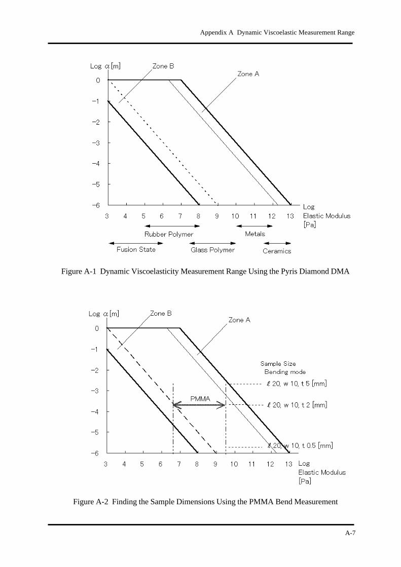
A-7
Appendix A Dynamic Viscoelastic Measurement Range
Figure A-1 Dynamic Viscoelasticity Measurement Range Using the Pyris Diamond DMA
Figure A-2 Finding the Sample Dimensions Using the PMMA Bend Measurement
A-8
A-3.3 Common Method of Finding the Sample Shape Using the Graph
The following is a common method for finding the appropriate sample size from this graph.
1. When the elasticity modulus of the sample is known
Plot the elasticity modulus of the sample (Pa) and the shape factor (m) on the graph. The
sample can be measured if the plotted point is within the two parallel lines.
Also, if the elsticity modulus of the sample will change due to temperature fluctuations
during the measurement, a curved line appears in the horizontal direction. Draw horizontal
dotted lines from the plotted point for the entire changing range of the elastic modulus and
make sure the entire range is within the parallelogram.
When it is outside or on the edge of the parallelogram, the sample shape must be changed.
When the sample shape is changed, the shape factor (m) also changes and the plotted point
moves in the up/down direction. Change the sample shape so the shape factor is in the
measurement range.
2. When the elasticity modulus of the sample is unknown
Place a sample with an appropriate shape into the instrument and click the Test button to
perform a test measurement. If the measurement is successfully completed, the results are
displayed in the measurement data window and the approximate elastic modulus of the
sample is known.
If the "A Low Zone Error occurred. (Is the sample too hard?)" message is displayed, change
the shape of the sample to reduce the sample factor α (m) and perform the measurement
again.
By performing these changes, the approximate elastic modulus of the sample can be
determined and the new value can be used in step 1 above to find the appropriate sample
shape.

A-9
Appendix A Dynamic Viscoelastic Measurement Range
Information
As shown in figure A-1, the Pyris Diamond DMA can continuously measure a sample with a
fixed shape across 5 columns of elastic modulus change. However, in the synthetic oscillation
mode, the upper limit of the AC power amplitude assigned to each frequency is 1/5 in comparison
to the sinusoidal osciallation mode. Because of this, there are times when measurements
cannot be peformed in the right 0.7 column (high elasticity Zone A). Furthermore, when
compared to other frequencies, the accuracy of tanδ, E" and E' may drop in the higher frequency
measurements of 20Hz for left column 1 (low elasticity Zone B).
1. The drop in accuracy of the E" and tanδ signal during phase difference
in high frequency measurements in zones B mentioned above is
particularly severe. For this reason, check the conformity of a lower
frequency measurement before using.
2. The measurement range shown in the parallelogram in Figure A-1 is
the region where the accuracy of the E’ measurement is within 30%,
the center is of higher accuracy than either the left or right sides. For
this reason, make sure the sample elastic modulus range is sufficiently
near the center of the parallelogram when determining the sample shape.
The upper value (Emax) and lower value (Emin) of the elasticity measurement using the Pyris
Diamond DMA can also be used to determine the equation numerically using the shape factor
(α) obtained in equations 1 ~ 4.
Emax = 107 / α (Pa), Emin = 102 / α (Pa)

A-10
B-1
Appendix B Static Viscoelasticity Measurement Range
Appendix B Static Viscoelasticity
Measurement Range
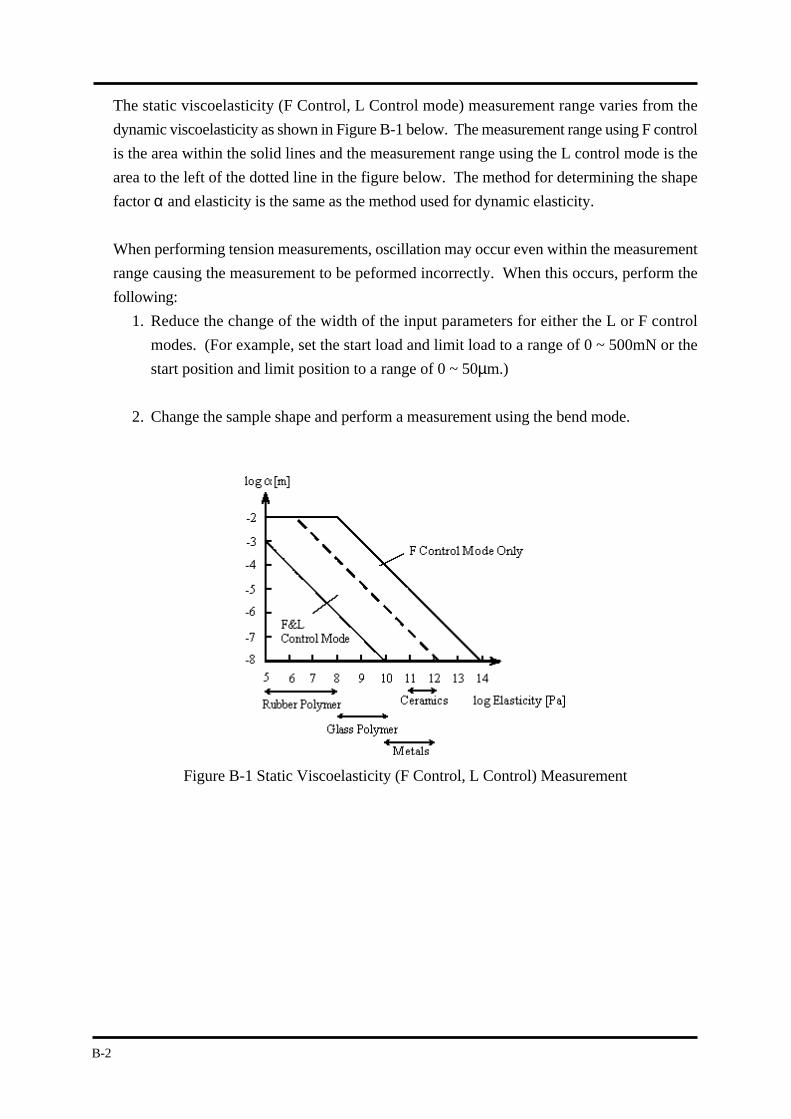
B-2
The static viscoelasticity (F Control, L Control mode) measurement range varies from the
dynamic viscoelasticity as shown in Figure B-1 below. The measurement range using F control
is the area within the solid lines and the measurement range using the L control mode is the
area to the left of the dotted line in the figure below. The method for determining the shape
factor α and elasticity is the same as the method used for dynamic elasticity.
When performing tension measurements, oscillation may occur even within the measurement
range causing the measurement to be peformed incorrectly. When this occurs, perform the
following:
1. Reduce the change of the width of the input parameters for either the L or F control
modes. (For example, set the start load and limit load to a range of 0 ~ 500mN or the
start position and limit position to a range of 0 ~ 50µm.)
2. Change the sample shape and perform a measurement using the bend mode.
Figure B-1 Static Viscoelasticity (F Control, L Control) Measurement
C-1
Appendix C Relationships Between the Various Quantities Used to Represent Dynamic Viscoelasticity
Appendix C Relationships Between the
Various Quantities Used to Represent
Dynamic Viscoelasticity
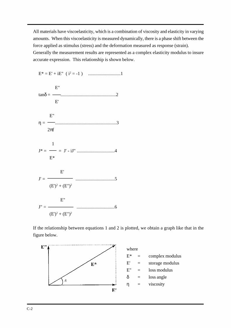
C-2
All materials have viscoelasticity, which is a combination of viscosity and elasticity in varying
amounts. When this viscoelasticity is measured dynamically, there is a phase shift between the
force applied as stimulus (stress) and the deformation measured as response (strain).
Generally the measurement results are represented as a complex elasticity modulus to insure
accurate expression. This relationship is shown below.
E* = E' + iE" ( i2 = -1 ) ...........................1
E"
tanδ = ..............................................2
E'
E"
η = ...................................................3
2πf
1
J* = = J' - iJ" ................................4
E*
E'
J' = .................................5
(E')2 + (E")2
E"
J" = ................................6
(E')2 + (E")2
If the relationship between equations 1 and 2 is plotted, we obtain a graph like that in the
figure below.
where
E* = complex modulus
E' = storage modulus
E" = loss modulus
δ = loss angle
η = viscosity
D-1
Appendix D Relationship Between Measurement Frequency and Transition Temperature
Appendix D Relationship Between
Measurement Frequency and
Transition Temperature
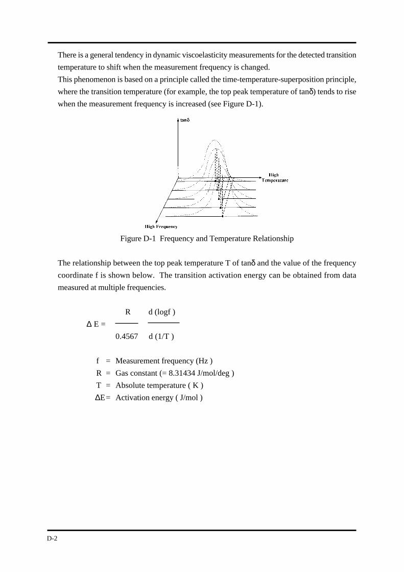
D-2
There is a general tendency in dynamic viscoelasticity measurements for the detected transition
temperature to shift when the measurement frequency is changed.
This phenomenon is based on a principle called the time-temperature-superposition principle,
where the transition temperature (for example, the top peak temperature of tanδ) tends to rise
when the measurement frequency is increased (see Figure D-1).
Figure D-1 Frequency and Temperature Relationship
The relationship between the top peak temperature T of tanδ and the value of the frequency
coordinate f is shown below. The transition activation energy can be obtained from data
measured at multiple frequencies.
R d (logf )
∆ E =
0.4567 d (1/T )
f = Measurement frequency (Hz )
R = Gas constant (= 8.31434 J/mol/deg )
T = Absolute temperature ( K )
∆E= Activation energy ( J/mol )
E-1
Appendix E Units Used in Measuring Viscoelasticity
Appendix E Units Used in Measuring
Viscoelasticity
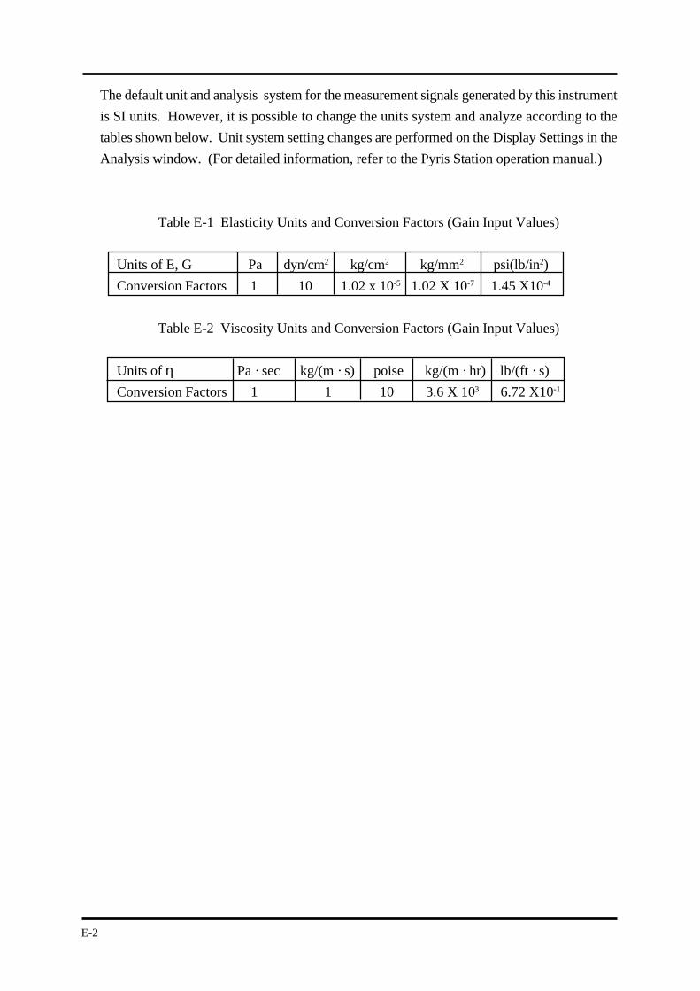
E-2
The default unit and analysis system for the measurement signals generated by this instrument
is SI units. However, it is possible to change the units system and analyze according to the
tables shown below. Unit system setting changes are performed on the Display Settings in the
Analysis window. (For detailed information, refer to the Pyris Station operation manual.)
Table E-1 Elasticity Units and Conversion Factors (Gain Input Values)
Units of E, G Pa dyn/cm2 kg/cm2 kg/mm2 psi(lb/in2)
Conversion Factors 1 10 1.02 x 10⁻⁵ 1.02 X 10⁻⁷ 1.45 X10⁻⁴
Table E-2 Viscosity Units and Conversion Factors (Gain Input Values)
Units of η Pa · sec kg/(m · s) poise kg/(m · hr) lb/(ft · s)
Conversion Factors 1 1 10 3.6 X 10³ 6.72 X10⁻¹
F-1
Appendix F Sample Temperature Signal Polynomial Regression Correction
Appendix F Sample Temperature Signal
Polynomial Regression Correction
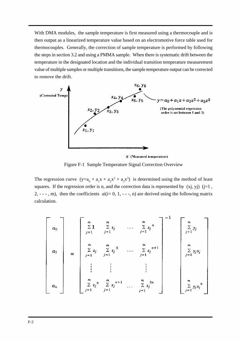
F-2
With DMA modules, the sample temperature is first measured using a thermocouple and is
then output as a linearized temperature value based on an electromotive force table used for
thermocouples. Generally, the correction of sample temperature is performed by following
the steps in section 3.2 and using a PMMA sample. When there is systematic drift between the
temperature in the designated location and the individual transition temperature measurement
value of multiple samples or multiple transitions, the sample temperature output can be corrected
to remove the drift.
Figure F-1 Sample Temperature Signal Correction Overview
The regression curve (y=a0 + a
1x + a
2x2 + a
3x3) is determined using the method of least
squares. If the regression order is n, and the correction data is represented by (xj, yj) (j=1 ,
2, - - - , m), then the coefficients ai(i= 0, 1, - - -, n) are derived using the following matrix
calculation.
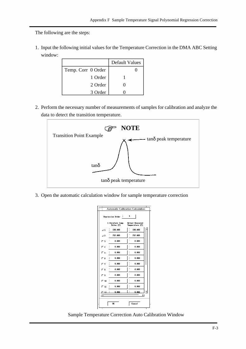
F-3
Appendix F Sample Temperature Signal Polynomial Regression Correction
NOTE
The following are the steps:
1. Input the following initial values for the Temperature Correction in the DMA ABC Setting
window:
Default Values
Temp. Corr 0 Order 0
1 Order 1
2 Order 0
3 Order 0
2. Perform the necessary number of measurements of samples for calibration and analyze the
data to detect the transition temperature.
Transition Point Example
tanδ
tanδ peak temperature
3. Open the automatic calculation window for sample temperature correction
Sample Temperature Correction Auto Calibration Window
tanδ peak temperature
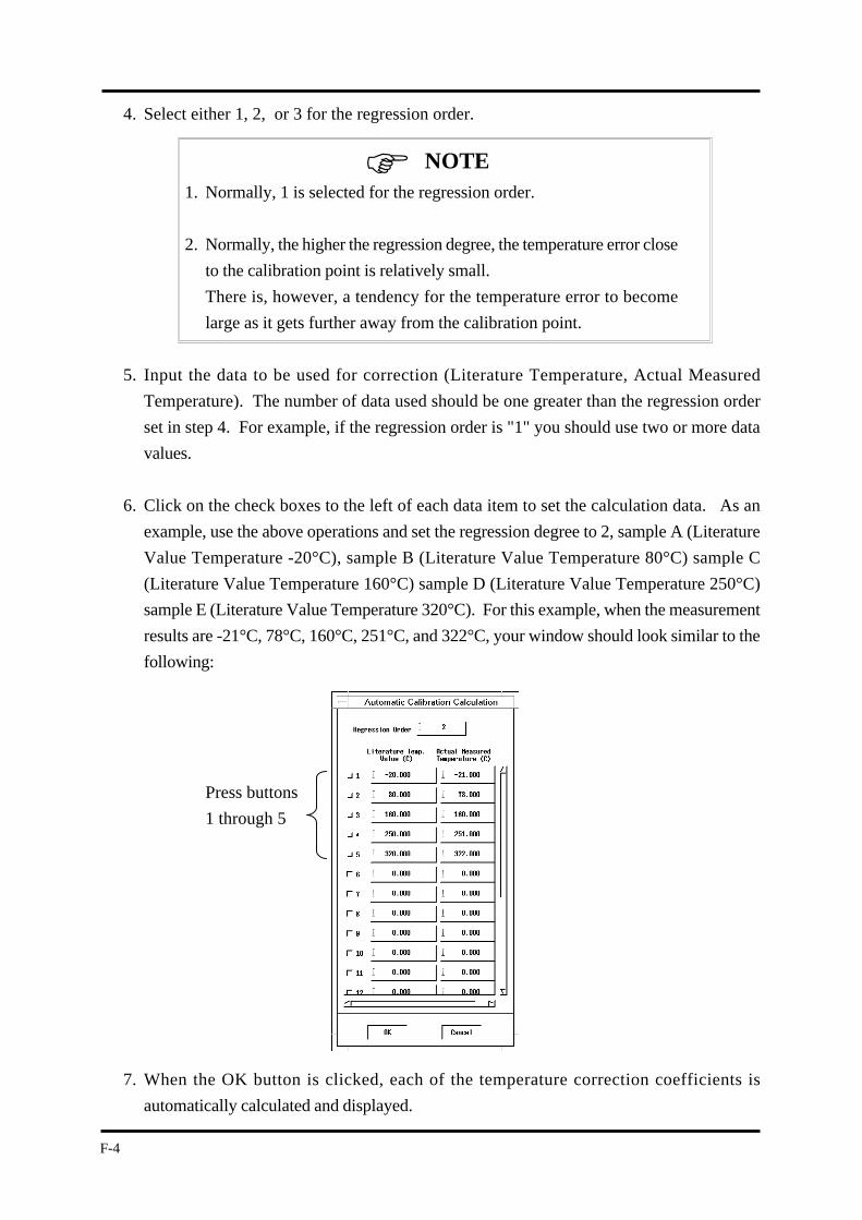
F-4
NOTE
4. Select either 1, 2, or 3 for the regression order.
1. Normally, 1 is selected for the regression order.
2. Normally, the higher the regression degree, the temperature error close
to the calibration point is relatively small.
There is, however, a tendency for the temperature error to become
large as it gets further away from the calibration point.
5. Input the data to be used for correction (Literature Temperature, Actual Measured
Temperature). The number of data used should be one greater than the regression order
set in step 4. For example, if the regression order is "1" you should use two or more data
values.
6. Click on the check boxes to the left of each data item to set the calculation data. As an
example, use the above operations and set the regression degree to 2, sample A (Literature
Value Temperature -20°C), sample B (Literature Value Temperature 80°C) sample C
(Literature Value Temperature 160°C) sample D (Literature Value Temperature 250°C)
sample E (Literature Value Temperature 320°C). For this example, when the measurement
results are -21°C, 78°C, 160°C, 251°C, and 322°C, your window should look similar to the
following:
Press buttons
1 through 5
7. When the OK button is clicked, each of the temperature correction coefficients is
automatically calculated and displayed.
G-1
Appendix G The Relationship Between Young's Modulus and Rigidity
Appendix G The Relationship Between
Young's Modulus and Rigidity
G-2
Young’s modulus (stretch or vertical elasticity coefficient) and the rigidity coefficient (shear
or horizontal elasticity coefficient) can be found with the DMA module, depending on the
measurement mode.
Bend, Tension, Compression Mode→ Young’s modulus measurement
Shear mode, Film Shear Mode → Rigidity coefficient measurement
The volume elasticity coefficient K, the Poisson ratio σ, Young’s modulus E, and the rigidity
coefficient G are all practical elasticity coefficients of isotropic materials. Only two of these
elasticity coefficients are independent. The others can be derived from them.
In other words,
EG
K = ..........................1
9G-3E
E - 2G
σ = ..........................2
2G
For many materials σ=0.5. If we apply this assumption to equation 2, we find that E=3G. This
relationship is called the "3-times rule of elasticity coefficients" and is very helpful in data
conversion
H-1
Appendix H Using the Optional Shear Attachment
Appendix H Using the Optional
Shear Attachment
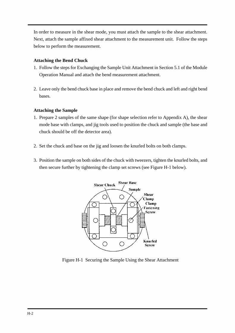
H-2
In order to measure in the shear mode, you must attach the sample to the shear attachment.
Next, attach the sample affixed shear attachment to the measurement unit. Follow the steps
below to perform the measurement.
Attaching the Bend Chuck
1. Follow the steps for Exchanging the Sample Unit Attachment in Section 5.1 of the Module
Operation Manual and attach the bend measurement attachment.
2. Leave only the bend chuck base in place and remove the bend chuck and left and right bend
bases.
Attaching the Sample
1. Prepare 2 samples of the same shape (for shape selection refer to Appendix A), the shear
mode base with clamps, and jig tools used to position the chuck and sample (the base and
chuck should be off the detector area).
2. Set the chuck and base on the jig and loosen the knurled bolts on both clamps.
3. Position the sample on both sides of the chuck with tweezers, tighten the knurled bolts, and
then secure further by tightening the clamp set screws (see Figure H-1 below).
Figure H-1 Securing the Sample Using the Shear Attachment
H-3
Appendix H Using the Optional Shear Attachment
Attachment to the Measurement Unit
1. Click the Motor Move icon, enter -1600µm for the Movement Target Position and click
the Move button. Set the probe to the 16mm position as with the bend measurement.
2. Attach the sample affixed shear attachment to the measurement unit. To attach the
attachment, secure the shear base to the brace using the 3mm hexagonal screws (4 screws)
and attach the shear chuck to the chuck base using the 2.5mm hexagonal screws (2 screws)
and tighten both.
Measurement
Select either Shear Sinusoidal or Shear Synthetic and set the measurement conditions paramaters
to correspond to the bend measurement and click the RUN button to begin the measurement.

H-4

I-1
Appendix I Using the Optional Compression Attachment
Appendix I Using the Optional
Compression Attachment
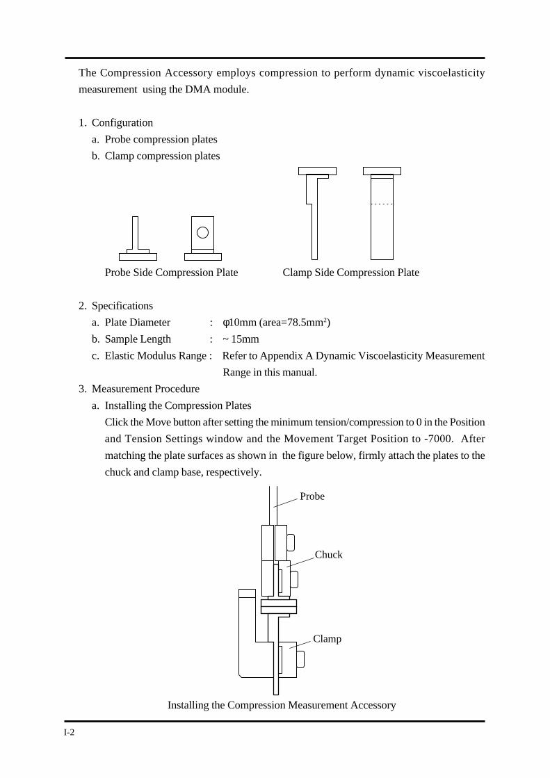
I-2
Probe
Chuck
Clamp
The Compression Accessory employs compression to perform dynamic viscoelasticity
measurement using the DMA module.
1. Configuration
a. Probe compression plates
b. Clamp compression plates
Probe Side Compression Plate Clamp Side Compression Plate
2. Specifications
a. Plate Diameter : φ10mm (area=78.5mm2)
b. Sample Length : ~ 15mm
c. Elastic Modulus Range : Refer to Appendix A Dynamic Viscoelasticity Measurement
Range in this manual.
3. Measurement Procedure
a. Installing the Compression Plates
Click the Move button after setting the minimum tension/compression to 0 in the Position
and Tension Settings window and the Movement Target Position to -7000. After
matching the plate surfaces as shown in the figure below, firmly attach the plates to the
chuck and clamp base, respectively.
Installing the Compression Measurement Accessory
I-3
Appendix I Using the Optional Compression Attachment
b. LVDT Signal Origin Adjustment
Click the Motor Move icon to open the window. Enter a value of -5000µm for the
Movement Target Position and click the Move button. The probe is moved to the -
5mm position. Enter 0 for the minimum tension/compression and click the OK button.
Input an offset load that will regulate the stress signal in the 0 ± 2µm range. The entered
offset value is shown in the window, after the window OK button is clicked.
c. Setting the Compression Conditions
Input the following conditions in the Position and Tension Settings window:
Min. Tension/Compression Force : 300mN
Tension/Compression Force Gain : 1.5
Force Amplitude Initial Value : 100mN
For compression measurements, use the following ranges:
Tension/Compression Force Gain : ≥ 0
d. Setting the Sample
Because it is necessary to keep the plates parallel when setting the sample, use the
movement target position setting and Move button.
1. Enter (sample length(mm) -7) x 1000 in the movement target position and click the
Move button.
2. Pinch the sample between the plates and click the TEST button to confirm that
measurement can be performed. Be sure that the sample is placed in the center
region of the plates.
I-4
NOTE
e. Starting Measurement
Open the Sample Condition setting window, enter the individual measurement conditions
and click the OK button. Click the TEST button and confirm that the elastic modulus is
an appropriate value for measurement. Next, close the furnace and press the RUN
button to start measurement.
1. Take note of the following information on the F force applied to the
sample.
F = Ft + F0 sin wt
Ft=Fbase+F0*F0 gain
Ft : oscillating force (the direction that pulls the sample
is positive)
F0 : constant force
Fbase : Min. Tension/Compression Force
F0 gain : Tension/Compression Gain
2. Using the Hold button, when measuring with the Automatic Cooling
Unit (optional accessory), may cause the sample to be pulled out and
dropped due to thermal contraction. For this reason, we suggest using
the RUN button instead. (When using RUN, a sample length
compensation mechanism is activated and the compression is
continuously applied to the sample according to the tension conditions
set previously .)
3. Poor contact between the sample surface and the compression plate
surface can cause large errors in the measurement values. When setting
the sample, be sure that the sample and plate surfaces are in full contact
with each other. If there is any uncertainty concerning the contact
status, we suggest the use of instant contact cement, etc. to fasten the
sample to the plate.
J-1
Appendix J Using the Optional Film Shear Attachment
Appendix J Using the Optional
Film Shear Attachment
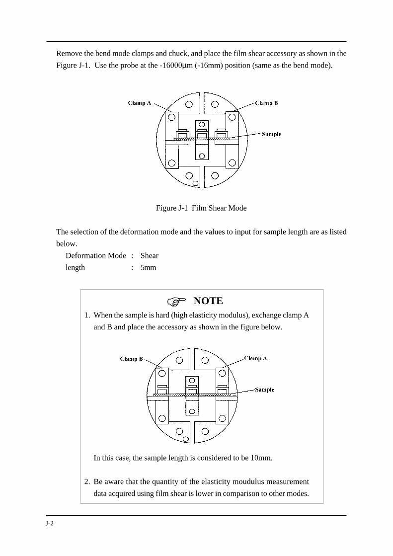
J-2
NOTE
Remove the bend mode clamps and chuck, and place the film shear accessory as shown in the
Figure J-1. Use the probe at the -16000µm (-16mm) position (same as the bend mode).
Figure J-1 Film Shear Mode
The selection of the deformation mode and the values to input for sample length are as listed
below.
Deformation Mode : Shear
length : 5mm
1. When the sample is hard (high elasticity modulus), exchange clamp A
and B and place the accessory as shown in the figure below.
In this case, the sample length is considered to be 10mm.
2. Be aware that the quantity of the elasticity moudulus measurement
data acquired using film shear is lower in comparison to other modes.
K-1
Appendix K Using the Optional Bend Attachment
Appendix K Using the Optional
Bend Attachment
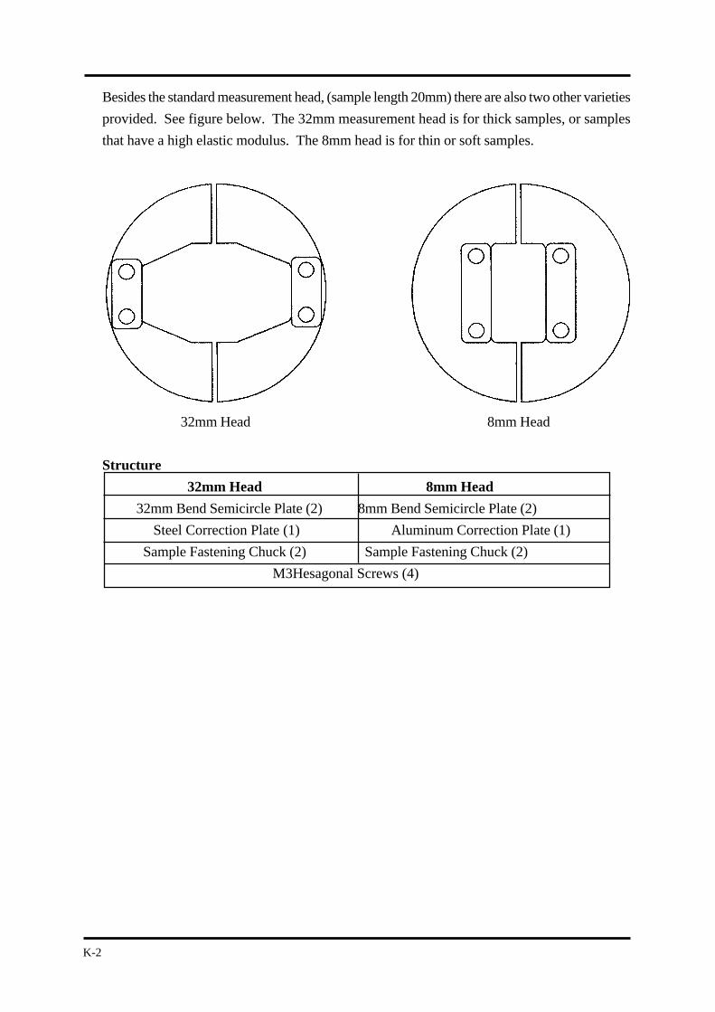
K-2
Besides the standard measurement head, (sample length 20mm) there are also two other varieties
provided. See figure below. The 32mm measurement head is for thick samples, or samples
that have a high elastic modulus. The 8mm head is for thin or soft samples.
32mm Head 8mm Head
Structure
32mm Head 8mm Head
32mm Bend Semicircle Plate (2) 8mm Bend Semicircle Plate (2)
Steel Correction Plate (1) Aluminum Correction Plate (1)
Sample Fastening Chuck (2) Sample Fastening Chuck (2)
M3Hesagonal Screws (4)
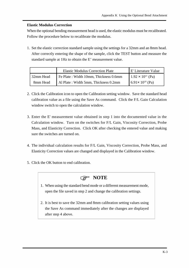
K-3
Appendix K Using the Optional Bend Attachment
NOTE
Elastic Modulus Correction
When the optional bending measurement head is used, the elastic modulus must be recalibrated.
Follow the procedure below to recalibrate the modulus.
1. Set the elastic correction standard sample using the settings for a 32mm and an 8mm head.
After correctly entering the shape of the sample, click the TEST button and measure the
standard sample at 1Hz to obtain the E’ measurement value.
Elastic Modulus Correction Plate E' Literature Value
32mm Head Fe Plate : Width 10mm, Thickness 0.6mm 1.92 × 10¹¹ (Pa)
8mm Head Al Plate : Width 5mm, Thickness 0.2mm 6.91× 10¹⁰ (Pa)
2. Click the Calibration icon to open the Calibration setting window. Save the standard head
calibration value as a file using the Save As command. Click the F/L Gain Calculation
window switch to open the calculation window.
3. Enter the E' measurement value obtained in step 1 into the documented value in the
Calculation window. Turn on the switches for F/L Gain, Viscosity Correction, Probe
Mass, and Elasticity Correction. Click OK after checking the entered value and making
sure the switches are turned on.
4. The individual calculation results for F/L Gain, Viscosity Correction, Probe Mass, and
Elasticity Correction values are changed and displayed in the Calibration window.
5. Click the OK button to end calibration.
1. When using the standard bend mode or a different measurement mode,
open the file saved in step 2 and change the calibration settings.
2. It is best to save the 32mm and 8mm calibration setting values using
the Save As command immediately after the changes are displayed
after step 4 above.

K-4
L-1
Appendix L Single-Cantilever Measurements
Appendix L Single-Cantilever
Measurements
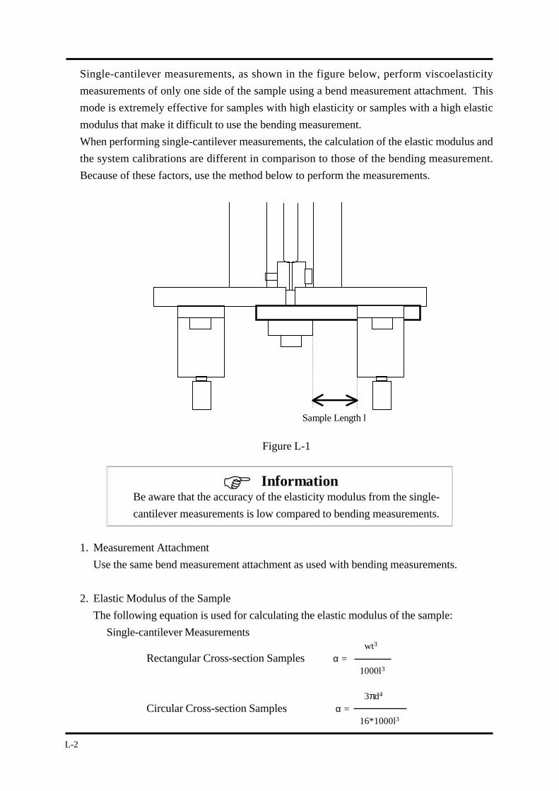
L-2
Information
Single-cantilever measurements, as shown in the figure below, perform viscoelasticity
measurements of only one side of the sample using a bend measurement attachment. This
mode is extremely effective for samples with high elasticity or samples with a high elastic
modulus that make it difficult to use the bending measurement.
When performing single-cantilever measurements, the calculation of the elastic modulus and
the system calibrations are different in comparison to those of the bending measurement.
Because of these factors, use the method below to perform the measurements.
Figure L-1
Be aware that the accuracy of the elasticity modulus from the single-
cantilever measurements is low compared to bending measurements.
1. Measurement Attachment
Use the same bend measurement attachment as used with bending measurements.
2. Elastic Modulus of the Sample
The following equation is used for calculating the elastic modulus of the sample:
Single-cantilever Measurements wt3
Rectangular Cross-section Samples α =1000l3
3πd4
Circular Cross-section Samples α =16*1000l3
Sample Length l
L-3
Appendix L Single-Cantilever Measurements
Information
α : Elastic Modulus (m) d : Sample diameter (mm)
t : Sample Thickness (mm) π : pi
w : Sample Width (mm) l : Sample length (mm)
For the sample length l, as shown in the figure above enter a value of 1/2 in relation to the
bending. For a 20mm bend attachment, enter 10mm. For a sample with the sample cross-
section shape, the calculation of the elastic modulus for the single-cantilever and bending
measurements, the single-cantilever will have a value of 1/2 that of the bending measurement.
In other words, the single-cantilever is 0.3 columns smaller and the elasticity measurement
range moves towards the high elasticity side by 0.3 columns. (Refer to Appendix A Dynamic
Viscoelasticity Measurement Range).
3. System Calibrations
a. Perform dynamic viscoelasticity measurement calibrations as outlined in Chapter 3 of
the Pyris Diamond DMA Operation Manual (Measurement Procedure) and save the
constants in a different file. If calibrations have already been performed, save as a
different file. If the file has already been saved, proceed to step b.
b. Open the saved constants file saved in step a.
c. Enter 0 for the compliance correction value. Do not change any other settings.
d. Using the Motor Move icon, set the target movement to -16000(µm) and click the
Move button. After movement is complete, click the OK button. Catching of a 12mm
width, 3mm thickness stainless plate, as shown in the figure for single-cantilevers is
performed.
Compliance calibrations can be performed from either the right or left
position. However, be sure to have the measurement position of the
sample the same as the calibration position. Likewise, the position
must be the same for sample temperature calibration.
e. Open the Sample Conditions setting window, perform the settings shown below and
click the OK button. (The bend attachment is being used but be aware that the
measurement mode selection is on shear.)
Control Mode Shear · Sinusoidal
Sample Shape Length : 0.01mm
Rectangular Cross-section
Width : 1mm
Thickness : 5.1mm
L-4
Information
Information
Data Filename Enter the appropriate filename (ex. dmscal.00)
Temperature Control Mode Step
Temperature Program
Soak : 2 (sec.)
Start Temp. : 0(°C)
Limit Temp. : 20
Frequency Setting 1Hz only ON
Stress Amplitude 20(µm)
f. Click the TEST button and perform a test measurement. After confirming the elasticity
displayed in the measurement data message window, click the OK button.
The test mode measurement functions to perform initialization of the
DMA control system.
g Click the Measure button and perform a measurement.
h. Once the measurement is complete, open the measured data using f slice analysis (ex.
dmscal.00). Set the X axis to time and calculate the average value of the G' value.
Using the signal properties window, signal selection and display settings
of f slice analysis, set the signal selection to G'Pa and make sure the A
(gain) and B (offset) coefficients on the lower left are set to 1 and 0
respectively.
If the values are different, enter A=1, B=0 and click the OK button.
Next, click the OK button on the Display Settings window.
i. Open the DMA ABC Setting window and click the Compliance Correction calculation
button.
In the Actual Value G' of the Auto Correction Calculation window read in the average
elasticity value (M') of G' from step e and click the OK button.
j. The value calculated in the compliance correction area is entered. If the value is correct,
the calculation value is in the 10-4 ~ 10-3 order. Click the OK button.
L-5
Appendix L Single-Cantilever Measurements
Be sure to close the window once using the OK button. If the window
is open, the correction will not be reflected in the steps that follow.
k. The value entered using the DMA ABC Setting window is the correction value for the
single-cantilever measurement. Save the file with a new name as a single-cantilever correct
value file.
4. Single-cantilever Measurements
The maximum length of the sample for single-cantilever measurements is 35mm. Enter the
measurement conditions using the Sample Condition Settings window. Enter a sample
length 1/2 that of the bend measurement attachment. When using a 20mm bend measurement
attachment, enter 10mm. For the measurement mode, select the Single-Cantilever Sinusoidal/
Synthetic control mode and click the OK button.
For sample chucking, secure the sample using the bend clamp on one side and the bend
chuck as shown in the figure. Be careful so that the sample is not touching another bend
clamp or the bend base.
When securing the bend chuck screw of the probe, hold the bend chuck
with your fingers so that the probe does not twist.
Click the Test button. After making sure the elasticity value is an appropriate value, close
the furnace, click the Measure button and begin the measurement.
Information
NOTE

L-6
M-1
Appendix M 3 Point Bending
Appendix M 3 Point Bending
Measurements
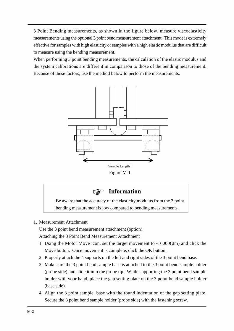
M-2
3 Point Bending measurements, as shown in the figure below, measure viscoelasticity
measurements using the optional 3 point bend measurement attachment. This mode is extremely
effective for samples with high elasticity or samples with a high elastic modulus that are difficult
to measure using the bending measurement.
When performing 3 point bending measurements, the calculation of the elastic modulus and
the system calibrations are different in comparison to those of the bending measurement.
Because of these factors, use the method below to perform the measurements.
Figure M-1
Be aware that the accuracy of the elasticity modulus from the 3 point
bending measurement is low compared to bending measurements.
1. Measurement Attachment
Use the 3 point bend measurement attachment (option).
Attaching the 3 Point Bend Measurement Attachment
1. Using the Motor Move icon, set the target movement to -16000(µm) and click the
Move button. Once movement is complete, click the OK button.
2. Properly attach the 4 supports on the left and right sides of the 3 point bend base.
3. Make sure the 3 point bend sample base is attached to the 3 point bend sample holder
(probe side) and slide it into the probe tip. While supporting the 3 point bend sample
holder with your hand, place the gap setting plate on the 3 point bend sample holder
(base side).
4. Align the 3 point sample base with the round indentation of the gap setting plate.
Secure the 3 point bend sample holder (probe side) with the fastening screw.
Information
Sample Length l
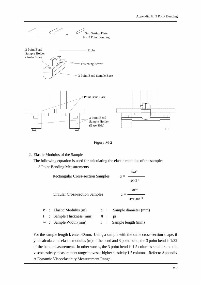
M-3
Appendix M 3 Point Bending
Figure M-2
2. Elastic Modulus of the Sample
The following equation is used for calculating the elastic modulus of the sample:
3 Point Bending Measurements 4wt3
Rectangular Cross-section Samples α =1000l 3
3πd4
Circular Cross-section Samples α =4*1000l 3
α : Elastic Modulus (m) d : Sample diameter (mm)
t : Sample Thickness (mm) π : pi
w : Sample Width (mm) l : Sample length (mm)
For the sample length l, enter 40mm. Using a sample with the same cross-section shape, if
you calculate the elastic modulus (m) of the bend and 3 point bend, the 3 point bend is 1/32
of the bend measurement. In other words, the 3 point bend is 1.5 columns smaller and the
viscoelasticity measurement range moves to higher elasticity 1.5 columns. Refer to Appendix
A Dynamic Viscoelasticity Measurement Range.
Gap Setting PlateFor 3 Point Bending
Probe
Fastening Screw
3 Point BendSample Holder(Probe Side)
3 Point Bend Sample Base
3 Point Bend Base
3 Point BendSample Holder(Base Side)
M-4
3. System Calibrations
a. Perform dynamic viscoelasticity measurement calibrations as outlined in Chapter 3 of
the Pyris Diamond DMA Operation Manual (Measurement Procedure) and save the
constants in a different file. If calibrations have already been performed, save as a
different file only. If the file has already been saved proceed to step b.
b. Open the saved constants file saved in step a.
c. Using the Motor Move icon, set the target movement to -15600(µm) and click the
Move button. After movement is complete, change the Force Amplitude value to 100mN
and click the OK button.
d. Place a steel plate as the sample with a width of 10mm and a thickness of 0.4mm.
e. Open the Sample Conditions setting window, perform the settings shown below and
click the OK button.
Sample Shape Length : 40mm
Rectangular Cross-section
Width : 10mm
Thickness : 0.4mm
Frequency Setting 1Hz only ON
Control Mode 3 Point Bending · Sinusoidal
Perform an actual measurement and enter the correct values for the
width and thickness of the steel plate.
f. Click the TEST button and perform a test measurement. After confirming the elasticity
displayed in the measurement data message window, click the OK button.
g. Click the Measure button and perform a measurement.
h. Once the measurement is complete, open the measured data using f slice analysis. Set
the X axis to time and read the E' value and calculate the average value.
i. Open the ABC Setting window and click the F/L Gain "Calculate" button.
j. Enter the following values into the Auto Calculate window:
Literature Value E' : 1.92 + 11
Actual Measured Value: Average value of E' calculated in step f.
Constant Update : Turn on F/L Gain, Viscosity Correction, Probe Mass,
and Elasticity Correction
Information
M-5
Appendix M 3 Point Bending
k. Click the OK button in the Auto Calculate window. The F/L Gain, Viscosity Correction,
Probe Mass, and Elasticity Correction values in the DMS ABC Setting window are
updated to the new values. Click the OK button.
l. The values entered into the DMS ABC Setting window are the 3 point bending corrected
values. Save this as a new file for the 3 point bending corrected file.
4. 3 Point Bending Measurements
Enter (sample length (mm) - 16) × 1000 for the target movement using the Motor Move
icon and click the Move button. Enter the other conditions and click the OK button. Open
the Sample Conditions Setting window and enter each measurement condition. Enter 40mm
for the sample length and select 3 point Bending Sinusoidal/Synthetic for the control mode.
Click the the OK button.
Set the sample and click the Test button. After making sure the elasticity value is an
appropriate value, close the furnace, click the Measure button to begin the measurement.

M-6
N-1
Appendix-N Tension/Compression Force During Tension/Compression Mode Measurements
Appendix-NTension/Compression Force During Tension/Compression Mode Measurements
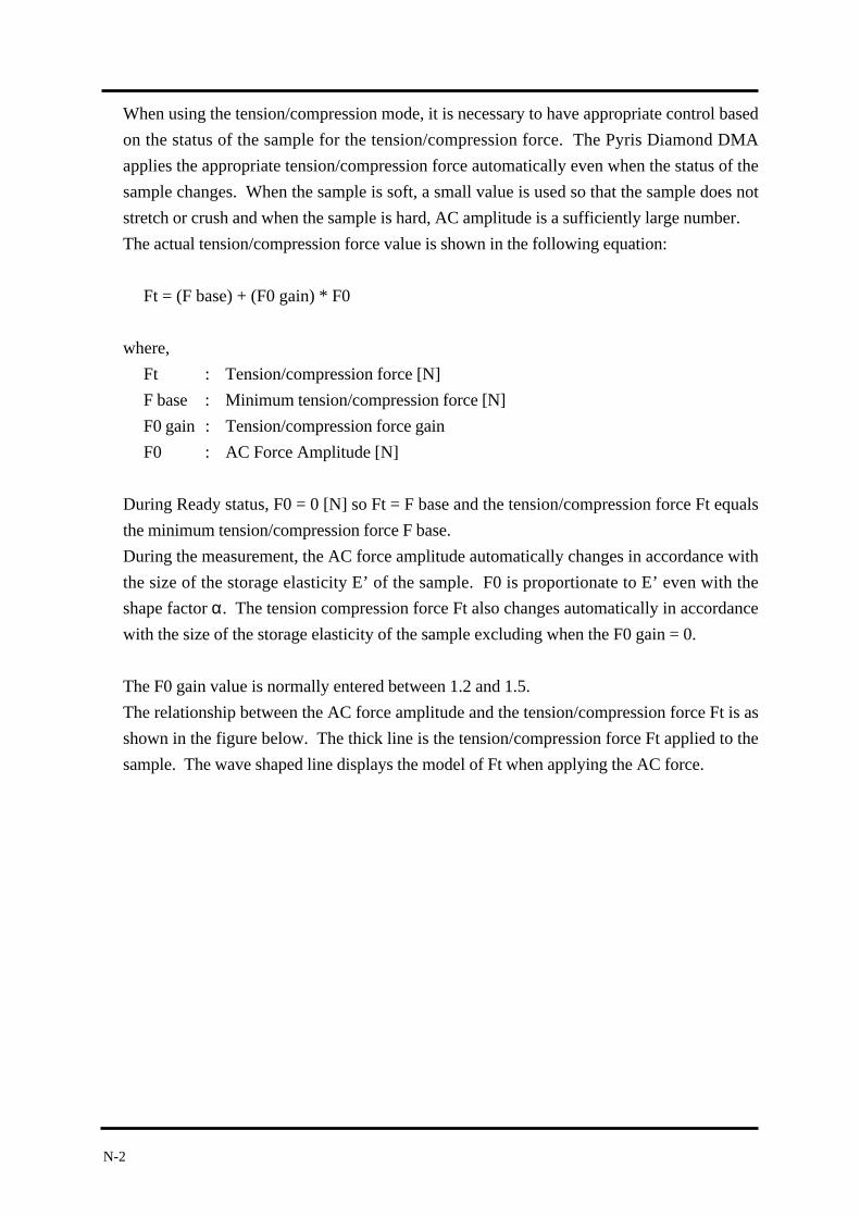
N-2
When using the tension/compression mode, it is necessary to have appropriate control based
on the status of the sample for the tension/compression force. The Pyris Diamond DMA
applies the appropriate tension/compression force automatically even when the status of the
sample changes. When the sample is soft, a small value is used so that the sample does not
stretch or crush and when the sample is hard, AC amplitude is a sufficiently large number.
The actual tension/compression force value is shown in the following equation:
Ft = (F base) + (F0 gain) * F0
where,
Ft : Tension/compression force [N]
F base : Minimum tension/compression force [N]
F0 gain : Tension/compression force gain
F0 : AC Force Amplitude [N]
During Ready status, F0 = 0 [N] so Ft = F base and the tension/compression force Ft equals
the minimum tension/compression force F base.
During the measurement, the AC force amplitude automatically changes in accordance with
the size of the storage elasticity E’ of the sample. F0 is proportionate to E’ even with the
shape factor α. The tension compression force Ft also changes automatically in accordance
with the size of the storage elasticity of the sample excluding when the F0 gain = 0.
The F0 gain value is normally entered between 1.2 and 1.5.
The relationship between the AC force amplitude and the tension/compression force Ft is as
shown in the figure below. The thick line is the tension/compression force Ft applied to the
sample. The wave shaped line displays the model of Ft when applying the AC force.
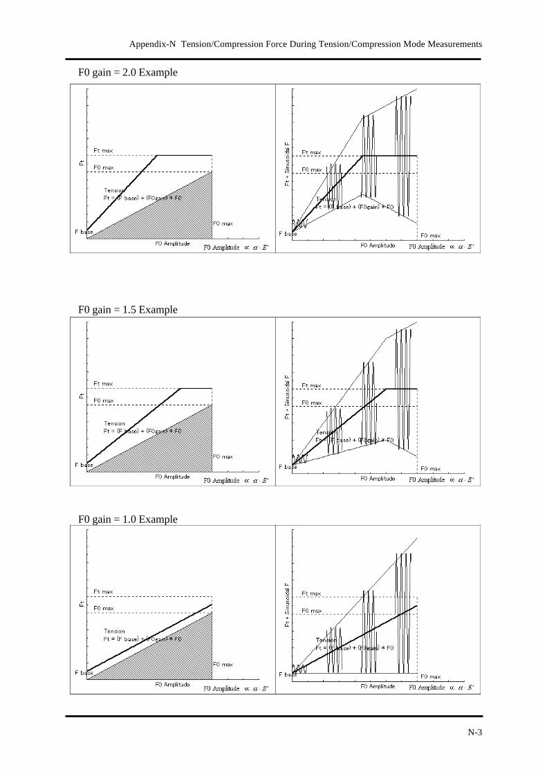
N-3
Appendix-N Tension/Compression Force During Tension/Compression Mode Measurements
F0 gain = 2.0 Example
F0 gain = 1.5 Example
F0 gain = 1.0 Example
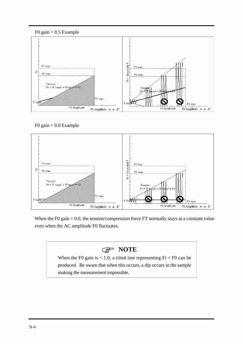
N-4
F0 gain = 0.5 Example
F0 gain = 0.0 Example
When the F0 gain = 0.0, the tension/compression force FT normally stays at a constant value
even when the AC amplitude F0 fluctuates.
When the F0 gain is < 1.0, a tilted line representing Ft < F0 can be
produced. Be aware that when this occurs, a dip occurs in the sample
making the measurement impossible.
NOTE