Embed Size (px)
Citation preview

Pyrolysis of wood powder and gasification of wood-derivedcharCitation for published version (APA):Guo, J. (2004). Pyrolysis of wood powder and gasification of wood-derived char. Eindhoven: TechnischeUniversiteit Eindhoven. https://doi.org/10.6100/IR577018
DOI:10.6100/IR577018
Document status and date:Published: 01/01/2004
Document Version:Publisher’s PDF, also known as Version of Record (includes final page, issue and volume numbers)
Please check the document version of this publication:
• A submitted manuscript is the version of the article upon submission and before peer-review. There can beimportant differences between the submitted version and the official published version of record. Peopleinterested in the research are advised to contact the author for the final version of the publication, or visit theDOI to the publisher's website.• The final author version and the galley proof are versions of the publication after peer review.• The final published version features the final layout of the paper including the volume, issue and pagenumbers.Link to publication
General rightsCopyright and moral rights for the publications made accessible in the public portal are retained by the authors and/or other copyright ownersand it is a condition of accessing publications that users recognise and abide by the legal requirements associated with these rights.
• Users may download and print one copy of any publication from the public portal for the purpose of private study or research. • You may not further distribute the material or use it for any profit-making activity or commercial gain • You may freely distribute the URL identifying the publication in the public portal.
If the publication is distributed under the terms of Article 25fa of the Dutch Copyright Act, indicated by the “Taverne” license above, pleasefollow below link for the End User Agreement:www.tue.nl/taverne
Take down policyIf you believe that this document breaches copyright please contact us at:[email protected] details and we will investigate your claim.
Download date: 11. May. 2020

PYROLYSIS OF WOOD POWDER AND GASIFICATION OF
WOOD-DERIVED CHAR
By
Jieheng Guo

Copyright c©2004 J.GuoOmslagontwerp: Paul Verspaget, Jieheng GuoDruk: Universiteitsdrukkerij, TUE
All rights reservedNo part of this work may be reproduced or transmitted in any form or byany means, electronic or mechanical, including photocopying, recording,or any information storage and retrieval system, without the permissionof the copyright owner.
CIP-DATA LIBRARY TECHNISCHE UNIVERSITEIT EINDHOVEN
Jieheng GuoPyrolysis of Wood Powder and Gasification of Wood-derived Char /by J.Guo. -Eindhoven: Technische Universiteit Eindhoven, 2004. -Proefschrift. - ISBN 90-386-1935-9NUR 961Trefw.: biomass, houtdeeltjes, houtskooldeeltjes, pyrolyse, vergassing,reactiekinetiek.Subject headings: biomass, wood powder, char, pyrolysis, gasification,reaction kinetics.
PYROLYSIS OF WOOD POWDER AND GASIFICATION OF
WOOD-DERIVED CHAR
PROEFSCHRIFT
ter verkrijging van de graad van doctor aan de
Technische Universiteit Eindhoven, op gezag van de
Rector Magnificus, prof.dr. R.A. van Santen, voor een
commissie aangewezen door het College voor
Promoties in het openbaar te verdedigen op
donderdag 17 juni 2004 om 16.00 uur
door
JIEHENG GUO
geboren te Shannxi, China

Dit proefschrift is goedgekeurd door de promotoren:
prof.dr.ir. M.E.H. van Dongen
en
prof.dr. W.R. Rutgers
Copromoter:
dr. A. Veefkind
The work presented in this thesis has been co-sponsored by The Centre Technology
for Sustainable Development (TDO) of the Eindhoven University of Technology
(TU/e) and the EU project NNE5-2001-00639. It is carried out within the
framework of the J. M. Burgerscentrum (JMBC), Research School for Fluid
Mechanics.

Table of Contents
Table of Contents v
1 Introduction 1
1.1 Why biomass gasification . . . . . . . . . . . . . . . . . . . . . . . . 1
1.2 Basic principles . . . . . . . . . . . . . . . . . . . . . . . . . . . . . . 2
1.3 State-of-the-art . . . . . . . . . . . . . . . . . . . . . . . . . . . . . . 4
1.4 Thesis overview . . . . . . . . . . . . . . . . . . . . . . . . . . . . . . 5
2 Materials and experimental methods 7
2.1 Raw biomass . . . . . . . . . . . . . . . . . . . . . . . . . . . . . . . 7
2.2 Chars . . . . . . . . . . . . . . . . . . . . . . . . . . . . . . . . . . . 10
2.2.1 Set-up and preparation procedure . . . . . . . . . . . . . . . 10
2.3 TGA experiments . . . . . . . . . . . . . . . . . . . . . . . . . . . . . 11
2.3.1 Set-up . . . . . . . . . . . . . . . . . . . . . . . . . . . . . . . 11
2.3.2 Analysis procedure . . . . . . . . . . . . . . . . . . . . . . . . 12
2.4 Grid reactor experiments . . . . . . . . . . . . . . . . . . . . . . . . 12
2.4.1 Configuration of the grid reactor . . . . . . . . . . . . . . . . 13
2.4.2 IR laser light absorption diagnostics . . . . . . . . . . . . . . 19
2.4.3 Data acquisition and processing . . . . . . . . . . . . . . . . 22
2.4.4 Measurement procedure . . . . . . . . . . . . . . . . . . . . . 23
2.4.5 Temperature measurement . . . . . . . . . . . . . . . . . . . 24
2.5 Shock tube technique . . . . . . . . . . . . . . . . . . . . . . . . . . . 29
v

2.5.1 Principle of shock tube . . . . . . . . . . . . . . . . . . . . . . 29
2.5.2 Conclusions from shock tube theory . . . . . . . . . . . . . . 31
2.5.3 Diagnostics . . . . . . . . . . . . . . . . . . . . . . . . . . . . 33
3 Characterization of chars 43
3.1 Introduction . . . . . . . . . . . . . . . . . . . . . . . . . . . . . . . . 43
3.2 Char samples . . . . . . . . . . . . . . . . . . . . . . . . . . . . . . . 43
3.3 Morphology of char . . . . . . . . . . . . . . . . . . . . . . . . . . . . 44
3.4 Physical adsorption of char . . . . . . . . . . . . . . . . . . . . . . . 45
3.4.1 Principle . . . . . . . . . . . . . . . . . . . . . . . . . . . . . 45
3.4.2 Apparatus and its analysis procedure . . . . . . . . . . . . . 46
3.5 Experimental Results . . . . . . . . . . . . . . . . . . . . . . . . . . . 48
3.6 Theoretical treatment . . . . . . . . . . . . . . . . . . . . . . . . . . 49
3.7 Conclusions . . . . . . . . . . . . . . . . . . . . . . . . . . . . . . . . 52
4 Fast pyrolysis of biomass at high temperature 53
4.1 Introduction . . . . . . . . . . . . . . . . . . . . . . . . . . . . . . . . 53
4.2 Pyrolysis characteristics of several biomasses . . . . . . . . . . . . . 54
4.3 High temperature pyrolysis in a shock tube reactor . . . . . . . . . . 58
4.3.1 Trajectories of wood particles in the shock tube . . . . . . . . 59
4.3.2 Heat transfer assessment . . . . . . . . . . . . . . . . . . . . . 66
4.3.3 Kinetics assessment . . . . . . . . . . . . . . . . . . . . . . . 69
4.3.4 Experimental results . . . . . . . . . . . . . . . . . . . . . . . 71
4.4 Conclusions . . . . . . . . . . . . . . . . . . . . . . . . . . . . . . . . 75
5 Gasification model 77
5.1 Introduction . . . . . . . . . . . . . . . . . . . . . . . . . . . . . . . . 77
5.2 Pore structure of char . . . . . . . . . . . . . . . . . . . . . . . . . . 78
5.3 C − CO2 gasification mechanism . . . . . . . . . . . . . . . . . . . . 79
5.4 Diffusive flow in chars: Dusty gas model . . . . . . . . . . . . . . . . 80
5.5 Model equations . . . . . . . . . . . . . . . . . . . . . . . . . . . . . 83
vi

5.5.1 Binary diffusion . . . . . . . . . . . . . . . . . . . . . . . . . . 83
5.5.2 Ternary diffusion . . . . . . . . . . . . . . . . . . . . . . . . . 86
5.6 Model predictions . . . . . . . . . . . . . . . . . . . . . . . . . . . . . 87
5.6.1 Binary case . . . . . . . . . . . . . . . . . . . . . . . . . . . . 88
5.6.2 Ternary case . . . . . . . . . . . . . . . . . . . . . . . . . . . 92
5.7 Conclusions . . . . . . . . . . . . . . . . . . . . . . . . . . . . . . . . 96
6 Gasification of the Lignocel-derived chars 99
6.1 Introduction . . . . . . . . . . . . . . . . . . . . . . . . . . . . . . . . 99
6.1.1 Review of literature . . . . . . . . . . . . . . . . . . . . . . . 100
6.2 Experimental scheme . . . . . . . . . . . . . . . . . . . . . . . . . . . 102
6.3 Experimental results . . . . . . . . . . . . . . . . . . . . . . . . . . . 103
6.3.1 Formation of nickel carbonyl on the reactor wall . . . . . . . 103
6.3.2 The effect of pyrolysis conditions on the char reactivity . . . 104
6.3.3 Gasification kinetics . . . . . . . . . . . . . . . . . . . . . . . 106
6.4 Conclusions . . . . . . . . . . . . . . . . . . . . . . . . . . . . . . . . 113
7 Concluding remarks and future work 115
7.1 Concluding remarks . . . . . . . . . . . . . . . . . . . . . . . . . . . 115
7.1.1 Fast pyrolysis in the shock tube reactor . . . . . . . . . . . . 115
7.1.2 Gasification in the grid reactor . . . . . . . . . . . . . . . . . 116
7.1.3 Gasification modelling . . . . . . . . . . . . . . . . . . . . . . 117
7.2 Future work . . . . . . . . . . . . . . . . . . . . . . . . . . . . . . . . 118
A Property data bank 121
B Temperature measurement by thermocouple 125
B.1 Evaluation of heat flow rates . . . . . . . . . . . . . . . . . . . . . . 125
B.2 Heat transfer coefficients and thermal conductivity . . . . . . . . . . 129
C Photo-detector response linearity 133
D TGA and DTG curves of biomass 135
vii
E Assessing kinetics parameters in external heat transfer controlled
regime 137
F Internal gas flow model 139
F.1 Structure of porous wood particle . . . . . . . . . . . . . . . . . . . . 139
F.2 Model equations . . . . . . . . . . . . . . . . . . . . . . . . . . . . . 140
F.3 Results and conclusions . . . . . . . . . . . . . . . . . . . . . . . . . 141
F.3.1 Pressure buildup . . . . . . . . . . . . . . . . . . . . . . . . . 142
F.3.2 Gas residence time . . . . . . . . . . . . . . . . . . . . . . . . 142
F.4 Appendix: Evaluation of R′s and C . . . . . . . . . . . . . . . . . . . 143
Bibliography 145
Summary 155
Samenvatting 157
Acknowledgement 159
Curriculum Vitae 161
viii

Chapter 1
Introduction
1.1 Why biomass gasification
Concerning the depletion of fossil fuels worldwide and the increasing environmentalpollution, numerous endeavors have been attempted to find other renewable andenvironmental friendly energy sources and to advance the technologies. As to thepower generation, biomass gasification technology becomes one of the most promis-ing technologies in the last two decades. Large scale application has two majoraspects.
First, biomass is a major source of energy for mankind and is presently estimatedto contribute of the order of 10%-14% of the world’s power supply[1]. Basically,biomass is an organic material, which includes plant, wood, crop residues, solidwaste, animal waste, sewage, and waste from food processing etc. It offers a numberof distinct advantages over other fossil fuels, in particular coal[2]. Biomass typicallypossesses a higher hydrogen content and a larger volatile component and producesa more reactive char after devolatilization. It contains lower ash and sulfur con-tents. Additionally, biomass, when grown and converted in a closed-loop feedstockproduction scheme, generates no net carbon dioxide emissions, thereby claiming aneutral position in the build-up of atmospheric greenhouse gases.
Second, gasification technology is an attractive route for the production of fuelgases from biomass. By gasification, solid biomass is converted into a combustiblegas mixture normally called “Producer Gas” consisting primarily of hydrogen (H2)and carbon monoxide (CO), with lesser amounts of carbon dioxide (CO2), water(H2O), methane (CH4), higher hydrocarbons (CxHy), nitrogen (N2) and particu-lates. The gasification is carried out at elevated temperatures, 800K-1700K, andat atmospheric or elevated pressures. The process involves conversion of biomass,
1

2 Chapter 1. Introduction
which is carried out in absence of air or with less air than the stoichiometric re-quirement of air for complete combustion. Partial combustion produces CO as wellas H2 which are both combustible gases. Solid biomass fuels, which are usually in-convenient and have low efficiency of utilization can thus be converted into gaseousfuel. The energy in producer gas is 70%-80% percent of the energy originally storedin the biomass[3]. The producer gas can serve in different ways: it can be burneddirectly to produce heat or used as a fuel for gas engines and gas turbines to generateelectricity; in addition, it can also be used as a feedstock (syngas) in the productionof chemicals e.g. methanol. The diversified applications of the producer gas makethe gasification technology very attractive.
1.2 Basic principles
A variety of biomass gasifiers has been developed. They can be grouped into fourmajor classifications[1,4,5]: fixed-bed updraft or counter current gasifier, fixed-beddowndraft or co-current gasifier, bubbling fluidized-bed and circulating fluidizedbed. Differentiation is based on the means of supporting the biomass in the reactorvessel, the direction of flow of both the biomass and oxidant, and the way heatis supplied to the reactor. The processes occurring in any gasifier include drying,pyrolysis, reduction, and oxidation. The unique feature of the updraft gasifier is thesequential occurrence of these processes: they are separated spatially and thereforetemporally. For this reason, the operation of an updraft gasifier will be used toillustrate the four processes. In Fig. 1.1 the reaction zones in an updraft gasifier
Fig. 1.1: Major processes occurring in an updraft gasifier cited from Warnecke[6].

1.2. Basic principles 3
are depicted. Biomass and air are fed in an opposite direction. In the highestzone, biomass is heated up and releases its moisture. In the pyrolysis zone, biomassundergoes a further increase in temperature and decomposes into hydrocarbons, gasproducts and char in the temperature range of 423K-773K[7]. The major reactionsare given as follows:
Biomassheat−→ CxHy + CxHyOz +H2O + CO2 + CO +H2 + etc.
The hydrocarbon fraction consists of methane to heavy tars (C1-C36 components).The composition of this fraction can be influenced by many parameters, such asparticle size of the biomass, temperature, pressure, heating rate, residence time,and catalysts[7]. The obtained char further reacts with the gas stream issuing fromthe oxidation zone in the reduction zone. Several important reactions occurring inthis zone are listed in Table 1.1. The first two reactions in Table 1.1 are usually
Table 1.1: Reactions occur in the oxidation zone.C + CO2 −→ 2CO 14H0 = 172 kJmol−1
C +H2O −→ H2 + CO 4H0 = 88 kJmol−1
C + 2H2O −→ H2 + CO2 4H0 = 130 kJmol−1
C + 2H2 −→ CH4 4H0 = −71 kJmol−1
CO +H2O −→ CO2 +H2 4H0 = −42 kJmol−1
CO + 3H2 −→ CH4 +H2O 4H0 = −205 kJmol−1
termed Boudouard and water-gas shift reactions, respectively. Both reactions arehighly endothermic and are favorable, kinetically and thermodynamically, at hightemperatures. The composition of the producer gases varies widely with the prop-erties of the biomass, the gasifying agent and the process conditions[7]. Dependingon the nature of the raw solid feedstock and the process conditions, the char formedfrom pyrolysis contains 20%-60% of the energy input[8]. Therefore the gasifica-tion of char is an important step for the complete conversion of the solid biomassinto gaseous products and for an efficient utilization of the energy in the biomass.The producer gases from the reduction zone rise beyond the reduction zone. Whenthey come into contact with the cooler biomass, the temperature drops down andthe aforementioned reactions are frozen. The unreacted char further undergoes theoxidation with air in the lowest zone and
C +O2 −→ CO2 4H0 = −390 kJmol−1 (1.2.1)
leaves ash at the bottom of the reactor. The produced CO2 flows upward and isinvolved in the reactions in the reduction zone. The heat released in the oxidationzone drives both the reduction and pyrolysis processes.
1determined at temperature of 298 K and at the pressure of 1 atm.

4 Chapter 1. Introduction
1.3 State-of-the-art
Gasification technology can achieve a high overall efficiency if it is integrated withthe gas cleaning, synthesis gas conversion and turbine power technologies. It istermed ”Integrated Gasification Combined Cycle” (IGCC). Large scale coal-firedIGCC plants have achieved a commercial status, as exemplified by the 250MWIGCC plant in Polk Power Station, USA, the 235MW plant at Buggenum, TheNetherlands, the 317.7MW plant at Puertollano, Spain etc. Biomass-fired IGCCtechnology, however, is still in an early phase of development and demonstrationand restricted to small scales. The world’s first biomass-fired IGCC plant is theVarnamo plant, which was built between 1991 and 1993. It is until now the onlycomplete and proven IGCC plant based on biomass. It can produce 6MWe
2 and9MWth
3 from wood chips. Other demonstration plants are still under constructionor at the early stage of commercialization such as the ARBRE plant ( 8MWe) inthe UK, the 12MWe demonstration plant in Italy and the 32MWe demonstrationplant in Brazil etc.
The main constraints to the commercialization of biomass-fired IGCC technologyare lack of confidence in the technology, technical and non-technical aspects[9, 10].The greatest technical challenge for the development of this technology, at all scales,continues to be adequately cleaning the tars and the particulates from the producergas such that the system operates efficiently and economically. Tar has to be re-moved from the producer gas before entering a gas turbine or an engine. This is notonly because of plugging of filters but also for many other reasons: (1) it condensesin exit pipes and plugs them, (2) it is very dangerous because of its carcinogeniccharacter, (3) it contains energy that can be transferred to the flue gas as H2, CO,CH4 etc., and (4) most gas engines and turbines do not accept tar in the incominggas. Particulates, if not removed beforehand, can cause serious damage to the bladesin turbines. Furthermore, there is no standard gasifier, which is able to handle awide range of fuel types. The quality of the producer gas is affected not only by thetypes of different gasifiers but also by treatment conditions such as temperature,pressure, hold time, heating rate (which is associated with the nature of biomass,particle size of the feed and temperature, etc.), pyrolysis atmosphere and so forth.
Reducing the production of tar and particulates in the gasification demands a thor-ough knowledge on the chemical kinetics of the gasification process. Informationabout how the reaction rate and product distribution are affected by the temper-ature, pressure, type of reactant gas, flow rate and the biomass properties is quiteimportant. Additionally, in practice, the chemical reactions may be coupled withthe transport phenomena e.g. the heat and mass transfer. Information about the
2MWe means megawatts electric.3MWth means megawatts thermal.
1.4. Thesis overview 5
interaction between the chemical kinetics and the transport phenomena are in turnessential to the optimal operation and a successful design of a gasifier.
The first stage of a logical design procedure requires the availability of reactionrate expressions (e.g. pyrolysis and gasification) that is appropriate for the rangeof conditions to be investigated in the design analysis. One requires knowledge ofthe dependence of the reaction rate on composition, temperature, fluid velocity, thecharacteristic dimensions of any heterogeneous phases present, and any other processvariables that may be significant. These information can be obtained by performingbench scale experiment, which are usually designed to operate at constant tempera-ture, under conditions that minimize heat and mass transfer limitations on reactionrates. This facilitates an accurate evaluation of the intrinsic chemical effects. Fur-thermore, in order to predict the gasification performance of the given feedstockand anticipate the technical problems, one has to employ a modelling tool, whichaccounts for all significant chemical reactions and physical processes. Through aninteraction between experimental experience and modelling, the most decisive fac-tors on determining the gasification rate parameters can finally be established. Thisforms the main scheme of the present work.
1.4 Thesis overview
The objective of this thesis is to provide practical data and a theoretical perspectiveabout the chemical kinetics and the transport phenomena in pyrolysis and gasifica-tion of biomass from both an experimental and a modelling perspective.
First, the basic information about the chemical composition of several biomass ma-terials will be given in Chapter 2. Additionally, the working principles and relevantdiagnostics of a number of experimental techniques will be depicted in greater de-tail. They are the shock tube reactor, the grid reactor and the thermogravimetricanalyzer. The char preparation procedure will also be specified. In relation to thechar gasification in the grid reactor, a char injector enabling depositing the charon a preheated grid and temperature measurement will be addressed. Concerningthe importance of the physical properties of the char, the morphology and the porestructure of the char will be independently dealt with in Chapter 3. There, theprinciple of the physical adsorption method and the characterization results will bepresented. Chapter 4 is specially focused on the derivation of chemical kinetics ofthe high temperature fast pyrolysis process. Chapter 5 is devoted to the modellingof the char gasification with CO2 and CO2/N2. The dusty gas model and the Lang-muir kinetics are incorporated to describe the diffusion of gaseous species and thereaction mechanism, respectively. In Chapter 6 experimental results on the influence

6 Chapter 1. Introduction
of the pyrolysis conditions on the char gasification reactivity and the intrinsic ki-netics of the char gasification with CO2 are highlighted. The role of diffusion is alsovalidated. Conclusions of the present study, together with some recommendations,are summarized in Chapter 7.

Chapter 2
Materials and experimentalmethods
An understanding of the structure and properties of biomass materials is necessaryin order to evaluate their utility as feedstocks for pyrolysis and gasification. Thischapter first summarizes available information on a variety of such properties in-cluding ultimate analysis, proximate analysis of biomass and chars by using thermalgravimetric analysis (TGA). Subsequently, the char preparation method is elabo-rated in section 2.2. To perform pyrolysis and gasification experiments, both thegrid reactor and the shock tube reactor are employed. The grid reactor is used toinvestigate the char gasification reactivity. The shock tube reactor is mainly usedto study the fast pyrolysis of biomass. These two setups were intensively used inthe past to study pulverized coal combustion and gasification at high temperaturesand high pressures[11, 12]. However, since the biomass properties differ from thoseof coal, the operating conditions as well as the diagnostics have been optimized tomeet the current needs. Therefore, in sections 2.4 and 2.5, the basic principles ofthe grid reactor and the shock tube are described as well as some improvements ofthe setup, diagnostic and the new data processing method.
2.1 Raw biomass
In this work a material named Lignocelr HB 120 was intensively used for inves-tigation of the pyrolysis and the gasification. It is a hard wood flour made by acomminution process yielding an average particle size of 120 µm.
The comminution process changes the physical structure of the wood. Typical hard-wood consists of long (l ∼ O(1mm)) hollow fiber tracheids which are connected with
7

8 Chapter 2. Materials and experimental methods
(a) (b)
Fig. 2.1: The structure of hard wood (a) [2] versus the structure of Lignocel (b).
each other through openings, referred to as pits as shown in Fig 2.1(a). In betweenthese tracheids, large vessels are present, with diameters of 20 to 30µm. During thecomminution, the physical structure of the original wood is destroyed. As can beseen in the SEM picture of Lignocel powder (Fig. 2.1(b)), it consists of fragments ofthe tracheids in which no pore structure in the order of µm is recognizable. Duringthe comminution process, the chemical structure of the wood is retained. Generally,woods can be separated into three fractions: extractables, cell wall components andash. The extractables, generally present in amounts of 4% to 20%, consist of ma-terial derived from the living cell. The cell wall components, representing the bulkof the cell, are principally the lingin fraction and the total carbohydrate fraction(cellulose and hemicellulose) termed holocellulose. Lignin, the cementing agent forthe cellulose fibers, is a complex polymer of phenylpropane. Cellulose is a poly-mer formed from d(+)-glucose while the hemicellulose polymer is based on otherhexose and pentose sugars. In woods the cell wall fraction generally consists oflignin/cellulose in the ratio 43/57[2]. The presence of the organic fraction: lignin,cellulose and hemicellulose, is expected to affect the overall reactivities for pyrolysisand gasification. To have a better understanding, two other materials: microcrys-talline Cellulose and organosolv Lignin are also examined. Organosolv Lignin wasobtained from Aldrich Chemical Company, WI, USA (Catalog No.: 37, 101 − 7).It is a polymeric organosolv lignin material isolated from a commercial pulp millusing mixed hardwood (mixture of 50% maple, 35% birch and 15% poplar) as rawmaterial. The microcrystalline cellulose was also obtained from Aldrich ChemicalCompany, WI, USA (Catalog No.: 43, 523−6). It is a purified, partially depolymer-ized cellulose, prepared by treating alpha-cellulose, obtained as a pulp from fibrous

2.1. Raw biomass 9
plant material, with mineral acids. The degree of polymerization is typically lessthan 400.
The ultimate and proximate analysis of samples as received are presented in Table2.1. The ultimate analysis generally reports the C, H, N , S and (by difference)O content in the sample. The proximate analysis classifies the sample in terms ofmoisture (M), volatile matter (VM), fixed carbon (FC) and mineral matter(ASH).The volatile matter mainly consists of the organic compounds. The moisture deter-mined by the proximate method represents the water that is bound physically to thematrix structure; water released by chemical reactions during pyrolysis is classifiedwith the volatiles. The ash content is determined by combustion of the volatile andfixed-carbon fractions. The resulting ash fraction is not representative for the ash inthe raw material, more appropriately termed mineral matter, due to the oxidationprocess employed in its determination. The fixed-carbon content is calculated fromthe material balance. Thus: FC = 1 − M − ASH − VM . The fixed carbon isconsidered to be a polynuclear aromatic hydrocarbon residue resulting from con-densation reactions which occur in the pyrolysis step. It not only contains carbonbut also some other elements such as oxygen, nitrogen and sulphur. To avoid effectsof moisture on the pyrolysis reaction, all the samples were kept at 323 K beforeanalysis.
Table 2.1: The ultimate and proximate analysis of all samples as received.
Ultimate(wt%, daf)
Cellulose Lignin Lignocel
C 47.23 72.53 53.67
H 5.80 5.43 5.36
N 0.00 0.00 0.00
S 0.00 0.00 0.00
O 46.97 22.04 40.97
Cl 0.00 0.00 0.00
Proximate (wt%)
Cellulose Lignin Lignocel
Moisture 4.30 2.61 9.45
Volatiles (daf1) 84.65 76.66 76.45
Fixed Carbon (daf) 11.05 20.73 13.56
Ash (dry) 0.00 0.00 0.54
1dry ash-free basis.

10 Chapter 2. Materials and experimental methods
2.2 Chars
2.2.1 Set-up and preparation procedure
The chars are prepared by pyrolyzing Lignocel wood under a continuous N2 flowwith a flow rate of 150ml min−1 in a furnace as shown in Fig. 2.2. About 0.4 g ofLignocel powder was put in a stainless steel sample container. Before the pyrolysiscommences, the sample container stays in the cold zone of a quartz tube, wherethe wood particles can be dried at T0 (typically 423K) denoted as prior to thepyrolysis process. Note that the drying temperature should not exceed 423K sothat no pyrolysis can take place. The furnace can be heated up to a maximum of1200K and can be stabilized at the required temperature under the control of athermostat. Due to the heat transfer between the quartz tube and the N2 flow, thetemperature of the sample can differ from that of the furnace. To check the exactgas temperature inside the quartz tube, a thermocouple is attached to the pipeduring N2 flow. When the required temperature TfT is achieved and stabilized, thesample container is rapidly pushed into the hot zone at time t0, when the pyrolysisof woods starts to take place. The released volatiles can be purged away by the N2
flow so that no secondary reactions occur. Another thermocouple is welded underthe sample container. It is used to measure the sample temperature. After a certainresidence time, the sample container is moved back to the cold zone at time tfT .There the produced chars are cooled down. Finally, the prepared chars are weighedand stored in glass bottles filled with N2 to avoid oxidation.
Fig. 2.2: Schematic diagram of the furnace.

2.3. TGA experiments 11
The pyrolysis hold time th is determined by the relation th = tfT − t0. The weightloss of the wood is ml = mw −mc, i.e. the difference between the initial weight ofwood and the weight of the char. Thus the conversion ratio can be calculated in thefollowing way,
Xc =ml
mw. (2.2.1)
The heating rate of this process is defined as,
βh =TfT − T0
tβ, (2.2.2)
where the parameter tβ is defined as tβ = tf − t0 and tf is the time when the sampletemperature reaches TfT . The conversion ratio is used as an index for evaluatingthe reproducibility of chars. Chars are taken as identical only if the difference inconversion ratio is less than 3%.
The pore structure of the char is an essential factor in determining the reactivityof the gasification. It can be measured by using a physical adsorption technique.Considering its importance, this part will be independently discussed in Chapter 3.
2.3 TGA experiments
Thermal gravimetric analysis is a thermal analysis technique used to determinechanges in sample weight as a function of temperature. It can also be used tostudy changes in sample weight as a function of time at a constant temperature(isothermal TGA). The analysis can be performed under nitrogen, in the presenceof air, or other reactive atmospheres. Another possible application of TGA is tostudy the pyrolysis kinetics of the biomass as described elsewhere [13–16]. In thisthesis work, it is mainly employed to perform the proximate analysis of both the rawmaterials and the derived chars. In this section, the configuration and the analysisprocedure of TGA are described.
2.3.1 Set-up
Pyrolysis experiments and proximate analysis are performed in a TA InstrumentsSDT 2960 (Simultaneous Differential Thermal Analyzer) at the group of ThermalPower Engineering, Department of Mechanical Engineering and Marine Technology,Delft University of Technology. Fig. 2.3 shows its configuration. This SDT hashorizontal sample carriers and the location of the thermocouple is just below thecrucible in the sample carrier. In order to account for buoyancy effects, a correc-tion curve with empty crucibles was first obtained and then subtracted from the

12 Chapter 2. Materials and experimental methods
experimental results. No lids were used on top of the crucibles. Temperature cal-ibration, baseline calibration and weight calibration experiments were done as toeach condition, according to the manufacturer-provided manual.
Fig. 2.3: Configuration of the TA Instruments SDT 2960.
2.3.2 Analysis procedure
Similar procedures are used to carry out the pyrolysis and proximate analysis of thesamples. As for the proximate analysis, it was carried out under Helium (99.99%) ata constant flow rate of 100mlmin−1. First, a sample of about 8-10mg was heatedup to 383K and kept at this temperature for 30min to remove moisture. Then itwas heated to 1173K at a heating rate of 20Kmin−1 and kept at that temperaturefor 30min before burning the char in air in order to determine the ash content. Oneexample of the proximate analysis for Lignocel is depicted in Fig. 2.4. It shows threesteps process: removal of moisture at the temperature below 383K, devolatilizationin the range of 500K-680K and combustion of the residue. From the change ofthe weight in the three steps, M , VM , FC and ASH content can be determined asillustrated in Fig. 2.4. The pyrolysis experiment follows a similar procedure as theproximate analysis, but with variable heating rates and final temperatures.
2.4 Grid reactor experiments
A grid reactor is employed to study the pyrolysis and the gasification of Lignocelwood and its derived char. It was constructed at Eindhoven University of Tech-nology for the purpose of investigating the gasification of coal-derived char at hightemperature (up to 1950K) and high pressure (up to 2.5MPa). To ensure the oc-currence of an isothermal char gasification experiment, the char sample needs to be

2.4. Grid reactor experiments 13
(a) (b)
Fig. 2.4: An example of the proximate analysis. The weight loss of Lignocel woodas a function of (a) temperature and (b) time.
?6 6
?6?6
M
VM
FCAsh
fed onto the reactor at constant temperature. To meet this requirement, an injectorwas installed onto the grid reactor (section 2.4.1). The reaction rate is determinedfrom the CO production. The concentration of CO is measured by means of aninfrared absorption method, which will be elaborated in section 2.4.2.
2.4.1 Configuration of the grid reactor
The configuration of the grid reactor is schematically shown in Fig. 2.5. It contains
(a) Top view (b) Side view.
Fig. 2.5: The grid reactor.
14 Chapter 2. Materials and experimental methods
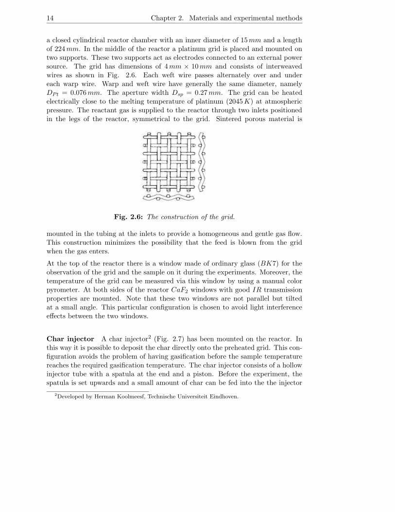
a closed cylindrical reactor chamber with an inner diameter of 15mm and a lengthof 224mm. In the middle of the reactor a platinum grid is placed and mounted ontwo supports. These two supports act as electrodes connected to an external powersource. The grid has dimensions of 4mm × 10mm and consists of interweavedwires as shown in Fig. 2.6. Each weft wire passes alternately over and undereach warp wire. Warp and weft wire have generally the same diameter, namelyDPt = 0.076mm. The aperture width Dsp = 0.27mm. The grid can be heatedelectrically close to the melting temperature of platinum (2045K) at atmosphericpressure. The reactant gas is supplied to the reactor through two inlets positionedin the legs of the reactor, symmetrical to the grid. Sintered porous material is
Fig. 2.6: The construction of the grid.
mounted in the tubing at the inlets to provide a homogeneous and gentle gas flow.This construction minimizes the possibility that the feed is blown from the gridwhen the gas enters.
At the top of the reactor there is a window made of ordinary glass (BK7) for theobservation of the grid and the sample on it during the experiments. Moreover, thetemperature of the grid can be measured via this window by using a manual colorpyrometer. At both sides of the reactor CaF2 windows with good IR transmissionproperties are mounted. Note that these two windows are not parallel but tiltedat a small angle. This particular configuration is chosen to avoid light interferenceeffects between the two windows.
Char injector A char injector2 (Fig. 2.7) has been mounted on the reactor. Inthis way it is possible to deposit the char directly onto the preheated grid. This con-figuration avoids the problem of having gasification before the sample temperaturereaches the required gasification temperature. The char injector consists of a hollowinjector tube with a spatula at the end and a piston. Before the experiment, thespatula is set upwards and a small amount of char can be fed into the the injector
2Developed by Herman Koolmeesf, Technische Universiteit Eindhoven.

2.4. Grid reactor experiments 15
tube and pushed onto the spatula by the piston. When the desired grid temperatureis reached, the injector tube is turned so that the chars can fall onto the grid. Thenit is pulled back to prevent the spatula from blocking the passage of the infrared
Fig. 2.7: A schematic picture of the char injector.
light. In Fig. 2.8 the pictures of the char particles dropped by the injector arepresented in the top and side views. It is seen that the particles are located in thecenter of the grid and packed up to around 1mm height. To ensure that this packedparticles are gasified isothermally, the following calculation is given with respect tothe heat-up process of the packed particles on the hot grid.
(a) Top view (b) Side view
Fig. 2.8: Top view and side view of char particles dropped by the injector.
For the gasification experiments, the char particles of diameter Dpc and height Hpc
are directly dropped onto the hot grid of height HPt that is held at a constanttemperature. On the grid, these particles are packed to a height of HB (see Fig.
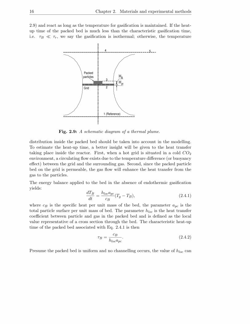
16 Chapter 2. Materials and experimental methods
2.9) and react as long as the temperature for gasification is maintained. If the heat-up time of the packed bed is much less than the characteristic gasification time,i.e. τB τr, we say the gasification is isothermal; otherwise, the temperature
5 4
3
1
2 H pt
(Reference)
Grid
H B
Packed particles
Fig. 2.9: A schematic diagram of a thermal plume.
distribution inside the packed bed should be taken into account in the modelling.To estimate the heat-up time, a better insight will be given to the heat transfertaking place inside the reactor. First, when a hot grid is situated in a cold CO2
environment, a circulating flow exists due to the temperature difference (or buoyancyeffect) between the grid and the surrounding gas. Second, since the packed particlebed on the grid is permeable, the gas flow will enhance the heat transfer from thegas to the particles.
The energy balance applied to the bed in the absence of endothermic gasificationyields:
dTB
dt=hlocapc
cB(Tg − TB), (2.4.1)
where cB is the specific heat per unit mass of the bed, the parameter apc is thetotal particle surface per unit mass of bed. The parameter hloc is the heat transfercoefficient between particle and gas in the packed bed and is defined as the localvalue representative of a cross section through the bed. The characteristic heat-uptime of the packed bed associated with Eq. 2.4.1 is then
τB =cB
hlocapc. (2.4.2)
Presume the packed bed is uniform and no channelling occurs, the value of hloc can

2.4. Grid reactor experiments 17
be estimated according to the following empirical correlation:[17]
jH = 0.91Re−0.51ψ, for Re < 50, (2.4.3)
jH = 0.61Re−0.41ψ, for Re > 50, (2.4.4)
where the Colburn jH factor and the Reynolds number are defined by
jH =hloc
cgρgu0(cgµg
kg)2/3f , (2.4.5)
Re =ρgu0
aψµf, (2.4.6)
where cg is the specific heat at constant pressure of the gas, ρg the density of thegas, a the surface area per unit volume of the bed, u0 is the superficial flow velocity.The shape factor ψ is taken as 0.91 for cylinders. In these equations the subscript fdenotes properties evaluated at the average temperature of gas and particle surface(0.5(Tps + TB)). The value of jH depends on the flow velocity. The buoyancy-induced flow velocity is estimated by means of an elementary natural convectionmodel. We assume that the temperature below the grid and of some distance asidefrom the grid are undisturbed with values T2 and so are the gas densities ρ2. Abovethe grid, the gas temperature is assumed to be T3 and equals the grid temperature.The density is assumed to be ρ3. Regime 3 is assumed to extend to the top wall ofthe reactor. At steady-state, the mechanical energy balance of the system (see Fig.2.9) can be described by
P1 = P2 +1
2ρ2u
20 + ρ2gh2, (2.4.7)
P3 = P4 + ρ4g(h4 − h3), (2.4.8)
P4 = P5, (2.4.9)
P5 = P1 − ρ2gh5. (2.4.10)
The gas flows through the grid and the packed particles due to a pressure drop thatcan be related to u0 by means of the Ergun equation[17,18]:
(P2 + ρ2gh2) − (P3 + ρ3gh3)
ρ2u20
(
Ds
HB
) (
ε3B1 − εB
)
=
[
150(1 − εB)
Dsρ2u0/µ2+ 1.75
]
, (2.4.11)
where Ds is the equivalent specific surface diameter defined as Ds = 6Vpc/apc.Combining Eqns.2.4.7-2.4.11 gives an implicit expression for u0:
[
0.5ρ2 + 1.75ρ2HB(1 − εB)
ε3BDs
]
u20 +
150µ2HB
ε3B
(
1 − εBDs
)2
u0 + (ρ3 − ρ2)gh4 = 0,
(2.4.12)

18 Chapter 2. Materials and experimental methods
where the subscript B represents the bed and HB the height of the bed.
If τB τr, a steady-state heat transfer analysis can be applied to further estimatethe intra-particle temperature difference induced by the endothermic gasification.We consider again a cylindrical particle. At steady state, the heat flow inward byconduction in the radial direction of cylinder must equal the energy consumptionby reaction. For one shell of a single particle in the bed, the energy balance is
−4H0DedC
dr= −ke
p
dTp
dr, (2.4.13)
where De is the effective diffusivity of the reactant gas, kep the effective thermal
conductivity of the particle, 4H0 the enthalpy of gasification. Negative signs arerequired on the left side of this equation so that for an endothermic reaction, thetemperature will be cooler in the core than at the periphery. Integration of theequation between the radius r and the gross particle radius Rp gives
Tp − Tps =4H0De
kep
(C − Cps), (2.4.14)
where Tps and Cps are the temperature and reactant concentration at the externalsurface of the char particle. The maximum temperature difference between thecenter of the particle Tpm = Tp(r = 0) and the external surface Tps(r = Rp) occurswhen the reactant concentration vanishes at r = 0.
Tpm − Tps = −4H0DeCps
kep
,
= −4H0DeP
RTpskep
, (2.4.15)
where P is the total pressure of the CO2 in the reactor.
The property values relevant to the grid and the packed bed are listed in Table2.2 and those of the char particle can be found in Appendix A. Substitution of
Table 2.2: Property values used in the estimation.
Parameter Value Parameter Value
Tps, K 600 - 1900 h4, m 2 × 10⁻²
P, Pa 1.01 × 10⁵ εB 0.6
Dpc, µm 10 CB, kJkg−1K−1 = cp(see AppendixA)
Hpc, µm 50 De, m2 s−1 10−7
4H0, kJmol−1 172[2]

2.4. Grid reactor experiments 19
the property values into the equations leads to a flow velocity of 0.11ms−1 anda characteristic heat-up time of the packed particles τB ≈ 21ms, which is muchless than the typical gasification time ranging from a few minutes to hours. Theintra-particle temperature difference is less than 1K. Therefore, it is reasonable toconsider the gasification of the char in the grid reactor as an isothermal reaction.
2.4.2 IR laser light absorption diagnostics
During the gasification of Lignocel with CO2, CO molecules are produced, whichdisperse in the closed volume of the grid reactor. The concentration of CO istime-dependent and can be used to calculate the reaction rate. The time-resolvedconcentration of CO can be detected by using an IR absorption technique.
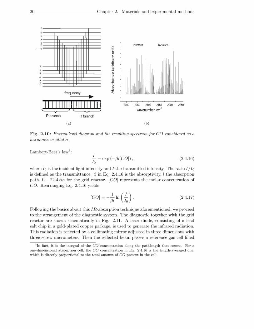
To begin with, the principle of the IR absorption technique is described briefly. Thistechnique relies on the fact that molecules absorb light (electromagnetic energy) atspectral regions where the radiated wavelength coincides with internal molecularenergy levels. In accordance to well known quantum mechanical theory such energyresonates with interatomic vibrations. At room temperature, the vibrational tran-sition is most often from the ground state to the first excited level. Accordingly,the vibrational spectrum of a diatomic molecule such as CO consists of one lineonly. For CO it is at 2143 cm−1. In addition to the absorption by the vibration, therotating oscillator can also absorb corresponding energy quantities exclusively forrotational excitation. Since the energy differences between rotational levels are somuch less than between vibrational ones, lines due to rotational transitions appearas fine structure near the frequency of the vibrational transition. In Fig. 2.10 theenergy levels and transitions for the vibration-rotation band of CO are depictedtogether with the resulting spectrum for CO. The absorption spectrum is based onthe HITRAN96 database. The spectrum consists of approximately equally spacedlines on each side of the center of the band. Transitions to the next higher energylevel (∆J = +1), counting from the J value of the lowest vibrational level, belongto the R branch and those with ∆J = −1 belong to the P branch. Transitionscorresponding to ∆J = 0 belong to the Q branch. But the Q branch does not occurfor gas phase CO at room temperature.
The diagnostic applied in the present work make use of a tunable infrared laser,which scans a very narrow wavelength region. Instead of the entire absorptionband the intensity of a single absorption line in the vibration-rotation spectrum isdetected and used as a representative of the CO concentration in accordance with
20 Chapter 2. Materials and experimental methods
(a) (b)
Fig. 2.10: Energy-level diagram and the resulting spectrum for CO considered as aharmonic oscillator.
Lambert-Beer’s law3:I
I0= exp (−βl[CO]) , (2.4.16)
where I0 is the incident light intensity and I the transmitted intensity. The ratio I/I0is defined as the transmittance. β in Eq. 2.4.16 is the absorptivity, l the absorptionpath, i.e. 22.4 cm for the grid reactor. [CO] represents the molar concentration ofCO. Rearranging Eq. 2.4.16 yields
[CO] = − 1
βlln
(
I
I0
)
. (2.4.17)
Following the basics about this IR-absorption technique aforementioned, we proceedto the arrangement of the diagnostic system. The diagnostic together with the gridreactor are shown schematically in Fig. 2.11. A laser diode, consisting of a leadsalt chip in a gold-plated copper package, is used to generate the infrared radiation.This radiation is reflected by a collimating mirror adjusted in three dimensions withthree screw micrometers. Then the reflected beam passes a reference gas cell filled
3In fact, it is the integral of the CO concentration along the pathlength that counts. For aone-dimensional absorption cell, the CO concentration in Eq. 2.4.16 is the length-averaged one,which is directly proportional to the total amount of CO present in the cell.

2.4. Grid reactor experiments 21
Fig. 2.11: The diagnostics of the grid reactor.
with CO of 933Pa. In front of the gas cell, a thin grating is coated. It splitsthe incident beam into two parts. One part of the beam passes through the gascell and is finally projected on a HgCdTe pn detector, which is cooled by liquidnitrogen to suppress thermal noise. The other part of the beam is expanded to aparallel beam with a diameter of 19mm. Then it passes the grid reactor throughtwo CaF2 windows with diameters of 15mm. So the CO in the entire volume can beirradiated. After passing the reactor, the transmitted light is projected on a secondHgCdTe pn detector. The light intensities received by two detectors in terms of thedetector voltages are transferred to a data acquisition system4.
The laser diode in our setup is cooled by liquid nitrogen and is tunable by modu-lating the current and adjusting the temperature. The current through the diodedetermines the wavelength range of the infrared radiation. The modulation currentperiodically changes the injection current from a value below threshold to another,thus the wavelength of the emitted radiation varies periodically. In this way a time-resolved spectrum can be obtained. The center wavelength of the laser dependson the temperature. Tuning the temperature can shift to another absorption line.Good thermal and electronic stability make sure that the spectrum scan emitted bythe diode laser is stable and reproducible. The modulation frequency determineshow many scans can be made. The maximum frequency is 20 kHz. It makes thissystem suitable for a fast process such as the pyrolysis as well as the slow processsuch as the gasification.
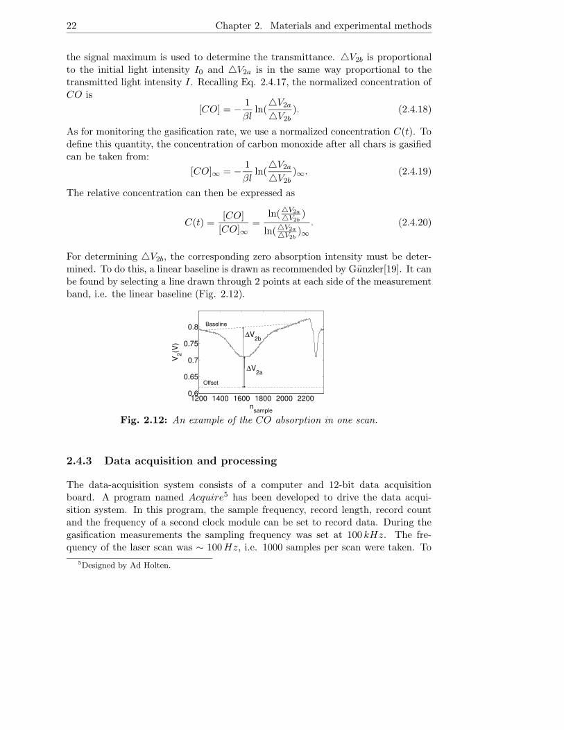
As described before the concentration of CO can be measured from the transmittedlight intensity(Eq. 2.4.17). To illustrate the calculation, an example of the trans-mission of CO in one scan is shown in Fig. 2.12. In this figure, the offset intensity iseasily determined by blocking the incident light into the detector. The intensity in
4This data acquisition system and the accompany software (Acquire) were built by Ad Holten,Technische Universiteit Eindhoven.
22 Chapter 2. Materials and experimental methods
the signal maximum is used to determine the transmittance. 4V2b is proportionalto the initial light intensity I0 and 4V2a is in the same way proportional to thetransmitted light intensity I. Recalling Eq. 2.4.17, the normalized concentration ofCO is
[CO] = − 1
βlln(
4V2a
4V2b). (2.4.18)
As for monitoring the gasification rate, we use a normalized concentration C(t). Todefine this quantity, the concentration of carbon monoxide after all chars is gasifiedcan be taken from:
[CO]∞ = − 1
βlln(
4V2a
4V2b)∞. (2.4.19)
The relative concentration can then be expressed as
C(t) =[CO]
[CO]∞=
ln(4V2a
4V2b)
ln(4V2a
4V2b)∞
. (2.4.20)
For determining 4V2b, the corresponding zero absorption intensity must be deter-mined. To do this, a linear baseline is drawn as recommended by Gunzler[19]. It canbe found by selecting a line drawn through 2 points at each side of the measurementband, i.e. the linear baseline (Fig. 2.12).
1200 1400 1600 1800 2000 22000.6
0.65
0.7
0.75
0.8
nsample
V2(V
)
∆V2a
∆V2b
Baseline
Offset
Fig. 2.12: An example of the CO absorption in one scan.
2.4.3 Data acquisition and processing
The data-acquisition system consists of a computer and 12-bit data acquisitionboard. A program named Acquire5 has been developed to drive the data acqui-sition system. In this program, the sample frequency, record length, record countand the frequency of a second clock module can be set to record data. During thegasification measurements the sampling frequency was set at 100 kHz. The fre-quency of the laser scan was ∼ 100Hz, i.e. 1000 samples per scan were taken. To
5Designed by Ad Holten.
2.4. Grid reactor experiments 23
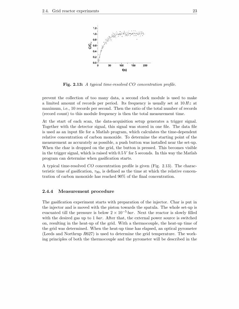
Fig. 2.13: A typical time-resolved CO concentration profile.
prevent the collection of too many data, a second clock module is used to makea limited amount of records per period. Its frequency is usually set at 10Hz atmaximum, i.e., 10 records per second. Then the ratio of the total number of records(record count) to this module frequency is then the total measurement time.
At the start of each scan, the data-acquisition setup generates a trigger signal.Together with the detector signal, this signal was stored in one file. The data fileis used as an input file for a Matlab program, which calculates the time-dependentrelative concentration of carbon monoxide. To determine the starting point of themeasurement as accurately as possible, a push button was installed near the set-up.When the char is dropped on the grid, the button is pressed. This becomes visiblein the trigger signal, which is raised with 0.5V for 5 seconds. In this way the Matlabprogram can determine when gasification starts.
A typical time-resolved CO concentration profile is given (Fig. 2.13). The charac-teristic time of gasification, τ90, is defined as the time at which the relative concen-tration of carbon monoxide has reached 90% of the final concentration.
2.4.4 Measurement procedure
The gasification experiment starts with preparation of the injector. Char is put inthe injector and is moved with the piston towards the spatula. The whole set-up isevacuated till the pressure is below 2 × 10⁻⁵ bar. Next the reactor is slowly filledwith the desired gas up to 1 bar. After that, the external power source is switchedon, resulting in the heat-up of the grid. With a thermocouple, the heat-up time ofthe grid was determined. When the heat-up time has elapsed, an optical pyrometer(Leeds and Northrup R627) is used to determine the grid temperature. The work-ing principles of both the thermocouple and the pyrometer will be described in the

24 Chapter 2. Materials and experimental methods
subsequent section 2.4.5. After these preparations, the data acquisition system isset on the status of ready and waiting for data. By means of the injector, the charis dropped onto the hot grid and the push button is pressed to trigger the data ac-quisition. The injector is pulled backwards immediately to prevent it from blockingthe laser light. After a predetermined time (which exceeds the time necessary tocomplete gasification), the recording of measurement data stops. The measurementis completed.
2.4.5 Temperature measurement
Optical pyrometer
The temperature of the hot grid is measured with an optical pyrometer (Leeds andNorthrup R627). This pyrometer operates with nearly monochromatic light. Thewavelength is usually a narrow band about 0.01 µm wide at 0.653 µm in the redportion of the visible spectrum. Radiation from the hot platinum grid is focused bythe lens onto a screen. The screen is viewed through a red filter glass so that onlywavelengths of about 0.653 µm are seen. Inside the pyrometer there is a tungstenwire which can be heated electrically. By making the brightness of the tungstenwire equal to that of the screen image of the grid, the temperature of the grid TPt
(K) can be measured. The temperature from the pyrometer Tb (K) is calibratedfor black body targets. The lower limit of the temperature range is about 1000K,determined by the long wave visibility limit of the human eye. When measuring thetemperature of the grid, a correction is necessary since it is a gray-body emitter.For a body of spectral emissivity ελ,T , at a temperature, T , and at a wavelength, λ,the monochromatic radiation intensity of the surface Iλ (W/m3 · sr) is
Iλ,T = ελ(λ, T )2hc2λ−5
exp(hc/(κλT )) − 1, (2.4.21)
where h = 6.6256×10⁻³⁴ Js is Planck’s constant, c is the speed of light propagationtaken as 2.998 × 10⁸m/s, κ = 1.3805 × 10⁻²³ J/K and ελ(λ, T ) is the emissivityof the body as a function of temperature and wavelength. As a gray-body, themonochromatic emissivity of the grid is independent of the wavelength and is equalto its total emissivity, namely
ελ(λ, T ) ∼= εtot(T ). (2.4.22)
Using this relation, the monochromatic radiation intensity of the platinum grid canbe correlated to the total emissivity of the platinum grid, εPt,tot. At the moment ofreading the measured temperature value, the brightness of the tungsten wire and of

2.4. Grid reactor experiments 25
the grid are equal. If the attenuation of incident radiation of the eyes and the lensesis negligible, the intensity of the wire and of the grid shall satisfy:
Ib(Tb) = IPt(TPt), (2.4.23)
In this equation, Tb corresponds to the reading of the pyrometer. Combining Eq.(2.4.23) with Eq. (2.4.21), we obtain
2hc2λ−5
exp( hcκλTb
) − 1= εPt,tot(
2hc2λ−5
exp( hcκλTPt
) − 1). (2.4.24)
Rewriting equation (2.4.24) we get
Tb =hcκλ
ln(1 − 1εPt
(1 − exp( hcκλTPt
))). (2.4.25)
By inserting the pairs of TPt and εPt,tot (see Table 2.3) into Eq. (2.4.25), thecorresponding Tb can be obtained. Fitting TPt versus Tb by linear regression yields
TPt = 1.151 ∗ Tb − 38.136. (2.4.26)
Table 2.3: Total emissivity of unoxidized platinum[20].
Temp., 0C 25 100 500 1000 1500
εPt,tot 0.037 0.047 0.096 0.152 0.191
Thermocouple
The optical pyrometer is limited to the high temperature regime, say T > 1000K.For the lower temperature regime, we use a type K (Chromel-Alumel) thermocouplewith a diameter of 0.2mm. Its measuring junction is clamped to the grid surface.The cold junction of this thermocouple is kept at the ice point. In order to inves-tigate the accuracy of the thermocouple measurement, a comparison between thesetwo methods has been made in the temperature range of 1100K and 1400K. Wefound that the measured temperature by the thermocouple was ∼ 200K lower thanthat measured by the pyrometer. This temperature deviation is attributed to adisturbance of the thermal field of the grid when introducing a thermocouple[21]. Asimilar problem has been well modelled by Keltner and Beck[22]. In this model, thethermocouple is supposed to be mounted on a thick wall. It is considered as a singlesemi-infinite cylinder with lateral surface heat loss characterized by a heat transfer

26 Chapter 2. Materials and experimental methods
coefficient, hc, with the ambient at the thermocouple temperature. It is assumedthat the heat flow rate and the temperature inside the thermocouple is constant in across-section. When the junction is just pressed against the surface of the substrateand has lateral heat loss, its steady-state temperature can be written as
Ttc =TPt
1 + 2K√Bi( 1
B + π4 ), (2.4.27)
with
K =kTc
kPt, B =
hptrTc
kPt, Bi =
hTcrTc
2kTc,
where k is the thermal conductivity, rTc is the thermocouple wire radius, α thethermal diffusivity, B the contact Biot number and Bi the lateral surface Biotmodulus. It is found that the accuracy of the measurement is only dependent onthe properties of the substrate and the thermocouple. According to Eq. 2.4.27, anestimate of TTc is performed with the parameters listed in Table 2.4. An example ofthe predicted temperature as a function of the thermocouple temperature is shown
Table 2.4: Parameters used for the estimation of Tgrid in Eq. 2.4.27.
Parameters K B Bi
Value 1 1 0.001
in Fig. 2.14. It is shown that the thermocouple technique could give rise to a 100Kdifference when the object temperature is over 1000K.
800 900 1000 1100 1200 1300 1400 1500800
900
1000
1100
1200
1300
1400
1500
1600
Ttc, K
T Pt,
K
Fig. 2.14: Prediction of the grid temperature as a function of the thermocoupletemperature according to Eq. 2.4.27.
2.4. Grid reactor experiments 27
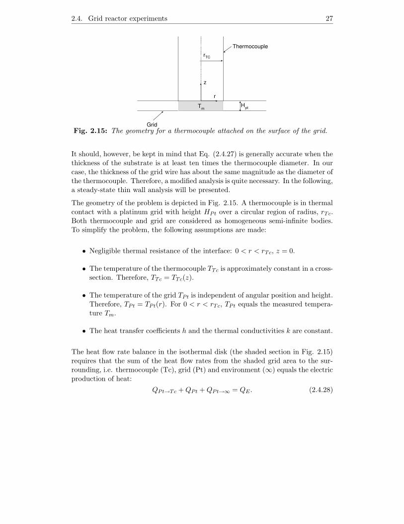
r TC
Thermocouple
Grid
z
r
T m H pt
Fig. 2.15: The geometry for a thermocouple attached on the surface of the grid.
It should, however, be kept in mind that Eq. (2.4.27) is generally accurate when thethickness of the substrate is at least ten times the thermocouple diameter. In ourcase, the thickness of the grid wire has about the same magnitude as the diameter ofthe thermocouple. Therefore, a modified analysis is quite necessary. In the following,a steady-state thin wall analysis will be presented.
The geometry of the problem is depicted in Fig. 2.15. A thermocouple is in thermalcontact with a platinum grid with height HPt over a circular region of radius, rTc.Both thermocouple and grid are considered as homogeneous semi-infinite bodies.To simplify the problem, the following assumptions are made:
• Negligible thermal resistance of the interface: 0 < r < rTc, z = 0.
• The temperature of the thermocouple TTc is approximately constant in a cross-section. Therefore, TTc = TTc(z).
• The temperature of the grid TPt is independent of angular position and height.Therefore, TPt = TPt(r). For 0 < r < rTc, TPt equals the measured tempera-ture Tm.
• The heat transfer coefficients h and the thermal conductivities k are constant.
The heat flow rate balance in the isothermal disk (the shaded section in Fig. 2.15)requires that the sum of the heat flow rates from the shaded grid area to the sur-rounding, i.e. thermocouple (Tc), grid (Pt) and environment (∞) equals the electricproduction of heat:
QPt→Tc +QPt +QPt→∞ = QE . (2.4.28)
28 Chapter 2. Materials and experimental methods
Derivation of each heat flow rate has been performed in Appendix B. Here, onlythe final solution with regard to the measured temperature Tm is given below:
Tm − T∞Tm − TPt,∞
=−
√
8hPtHPtkPt
r2Tc
K1(r′Tc)
K0(r′Tc
)− 2hPt
T∞−TPt,∞
Tm−TPt,∞
hPt +√
2hTckTc
rTc
. (2.4.29)
From this expression, it follows that the measured temperature depends on thephysical properties of both the grid and the thermocouple and also on their heattransfer coefficients. In the derivation of Eq. 2.4.29, all these quantities are assumedconstant. In reality, this might not be true. Especially, the overall heat transfercoefficient, which must include convection, conduction and radiation, is a functionof temperature. In this situation, the above relation is not valid anymore in a widetemperature range. Therefore, the temperature dependence of the heat transfercoefficients has to be investigated in the temperature range of our interest 800K-1600K. Also notice that in the above calculation, the grid is taken as a homogeneoussolid body. However, it in fact consists of weaved wires as depicted in Fig. 2.6. Thisconstruction gives rise to a larger area for heat transfer than a solid body and alsoto an effective heat conductivity different from that of the single wire.
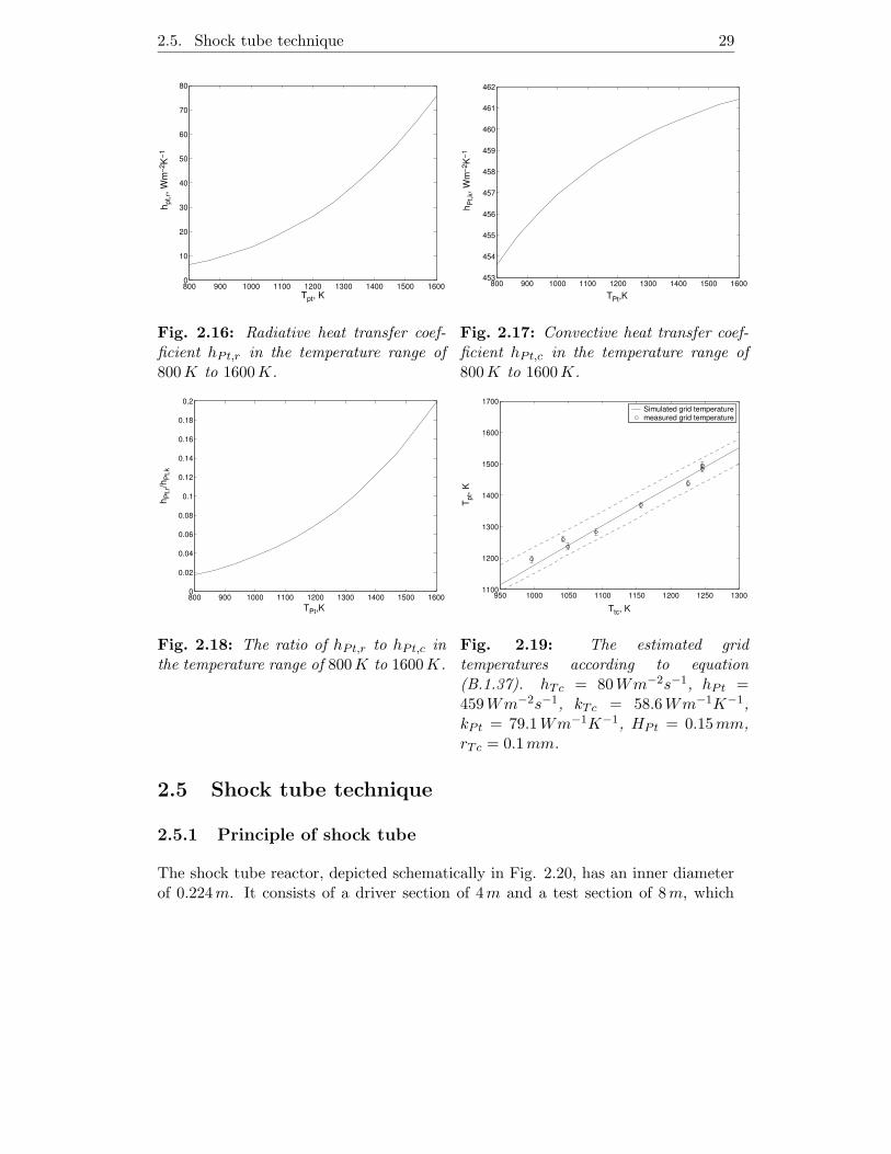
In Appendix B, the radiative heat transfer coefficient hPt,r, the convective heattransfer coefficient hPt,c and the thermal conductivity of the entire grid were eval-uated by taking into account the construction of the grid. Fig. 2.16 and Fig. 2.17show the temperature dependence of hPt,r and hPt,c, respectively. In the investi-gated temperature range, hPt,r changes rapidly with temperature. While, hPt,c isnearly constant. According to Fig. 2.18 the ratio of hPt,r to hPt,c is less than unity.Therefore, it is reasonable to state that the convective heat transfer is the domi-nating mechanism and is also constant in the temperature range of interest. Theauthor did not endeavor to estimate the heat transfer coefficient of the thermocou-ple. It is obtained by the following tryout procedure. Firstly, hPt = 459Wm−2s−1
and kPt = 79.1Wm−1K−1 were calculated respectively. Presuming a random valuefor hTc, a relationship between the estimated grid temperature and the thermocou-ple temperature was obtained. Of course, this relationship has to be verified by theexperimental data. By changing the current through the grid, the temperature waschanged accordingly and was measured by the pyrometer (TPt) and the thermocou-ple (Tm), respectively. The results are shown as the open circles in Fig. 2.19. The95% confidence interval of these data are plotted as the dashed line. Giving hTc
an initial value, a linear curve between TPt and Tm was obtained according to Eq.2.4.29. The final relationship was determined when the predicted values of TPt fallwithin the 95% confidence interval, yielding a hTc value of 80Wm−2s−1. At thegrid temperatures above 1000K, the temperatures estimated by Eq. 2.4.29 agreeswell with the those measured by the pyrometer.
2.5. Shock tube technique 29
800 900 1000 1100 1200 1300 1400 1500 16000
10
20
30
40
50
60
70
80
Tpt, K
hpt
,r, W
m−2
K−1
Fig. 2.16: Radiative heat transfer coef-ficient hPt,r in the temperature range of800K to 1600K.
800 900 1000 1100 1200 1300 1400 1500 1600453
454
455
456
457
458
459
460
461
462
TPt,K
h Pt,k
, Wm
−2K
−1
Fig. 2.17: Convective heat transfer coef-ficient hPt,c in the temperature range of800K to 1600K.
800 900 1000 1100 1200 1300 1400 1500 16000
0.02
0.04
0.06
0.08
0.1
0.12
0.14
0.16
0.18
0.2
TPt,K
h Pt,r
/hP
t,k
Fig. 2.18: The ratio of hPt,r to hPt,c inthe temperature range of 800K to 1600K.
950 1000 1050 1100 1150 1200 1250 13001100
1200
1300
1400
1500
1600
1700
Ttc, K
T pt,
K
Simulated grid temperaturemeasured grid temperature
Fig. 2.19: The estimated gridtemperatures according to equation(B.1.37). hTc = 80Wm−2s−1, hPt =459Wm−2s−1, kTc = 58.6Wm−1K−1,kPt = 79.1Wm−1K−1, HPt = 0.15mm,rTc = 0.1mm.
2.5 Shock tube technique
2.5.1 Principle of shock tube
The shock tube reactor, depicted schematically in Fig. 2.20, has an inner diameterof 0.224m. It consists of a driver section of 4m and a test section of 8m, which
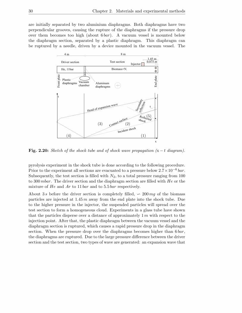
30 Chapter 2. Materials and experimental methods
are initially separated by two aluminium diaphragms. Both diaphragms have twoperpendicular grooves, causing the rupture of the diaphragms if the pressure dropover them becomes too high (about 6 bar). A vacuum vessel is mounted belowthe diaphragm section, separated by a plastic diaphragm. This diaphragm canbe ruptured by a needle, driven by a device mounted in the vacuum vessel. The
Fig. 2.20: Sketch of the shock tube and of shock wave propagation (x− t diagram).
(1)
(2)(3)
(4)
(5)
pyrolysis experiment in the shock tube is done according to the following procedure.Prior to the experiment all sections are evacuated to a pressure below 2.7×10⁻⁶ bar.Subsequently, the test section is filled with N2, to a total pressure ranging from 100to 300mbar. The driver section and the diaphragm section are filled with He or themixture of He and Ar to 11 bar and to 5.5 bar respectively.
About 3 s before the driver section is completely filled, v 200mg of the biomassparticles are injected at 1.45m away from the end plate into the shock tube. Dueto the higher pressure in the injector, the suspended particles will spread over thetest section to form a homogeneous cloud. Experiments in a glass tube have shownthat the particles disperse over a distance of approximately 1m with respect to theinjection point. After that, the plastic diaphragm between the vacuum vessel and thediaphragm section is ruptured, which causes a rapid pressure drop in the diaphragmsection. When the pressure drop over the diaphragms becomes higher than 6 bar,the diaphragms are ruptured. Due to the large pressure difference between the driversection and the test section, two types of wave are generated: an expansion wave that

2.5. Shock tube technique 31
travels towards the front plate and a compression shock wave (incident shock wave)that pushes the test gas towards the end plate. The wave pattern is depicted in thex− t diagram in Fig. 2.20. It starts when the aluminium diaphragms are ruptured.In the x− t diagram, regions (1) and (4) are the initial states of the test section andthe driver section, respectively. Region (2) is the state behind the incident shock.The test gas behind the incident shock is compressed to a pressure range of 1−2 barand a temperature range of 500− 1000K. The contact surface separates the drivergas and the test gas. Its velocity is lower than the incident shock velocity. Whenthe incident shock reaches the end plate, it is reflected. The test gas behind thereflected shock forms a stagnation region. Typical gas conditions in this region are7−10 bar and 950−1500K. The pyrolysis of the particles takes place in this region.At a certain time, the reflected shock meets the contact surface. Depending on theconditions, different events may occur. A particular situation arises when there isno reflected wave at all: the ’tailored’ interface condition. In general, the reflectedshock will partly penetrate region (3) and will partly be reflected from the contactsurface as a shock wave or as an expansion fan. These waves affect the stagnationconditions which will be discussed later.
The stagnation conditions will be destroyed anyhow when the head of the expansionwave, reflected from the front plate, arrives. The total test time, ttest is defined asthe time between the creation of the reflected shock wave and the arrival of the headof the expansion wave. It has a typical value of about 4ms.
The stagnation conditions depend on the initial pressure ratio and the compositionof the test gas and the driver gas. The state change satisfies elementary conservationlaws such that a simple measurement of the incident shock velocity at known initialconditions is sufficient to calculate the velocity, temperature, pressure and densityin each region shown in Fig, 2.20. The incident shock velocity is determined by thetime difference of the arrival of the incident shock at three transducers placed atdifferent positions along the shock tube. The principle of this calculation is basedon the shock theory explained elsewhere [11, 12, 23]. In the following subsection,only the results are summarized.
2.5.2 Conclusions from shock tube theory
The following conclusions are derived on the basis of one-dimensional shock tubetheory described in reference [23].

32 Chapter 2. Materials and experimental methods
Relations between regions (1) and (2) The gas velocity behind the incidentshock u2 reads
u2 =
2a1
γ1+1
Ms1 − 1Ms1
, (2.5.1)
where Ms1 = Us1/a1 is the shock wave Mach number and a1 the sound velocity inthe test gas in state 1, given by [23]
a1 =
√
γ1RT1
MN2
. (2.5.2)
γ is the adiabatic exponent. It equals 5/3 for a monatomic gas and 7/5 for a diatomicgas. The shock jump relations for density, pressure and temperature can be writtenas follows
ρ2
ρ1=
(γ1 + 1)M2s1
2 + (γ1 − 1)M2s1
, (2.5.3)
P2
P1= 1 +
2γ1
γ1 + 1(M2
s1 − 1), (2.5.4)
T2
T1= 1 +
2(γ1 − 1)
(γ1 + 1)2γ1M
2s1 − 1
M2s1
(M2s1 − 1). (2.5.5)
Reflection of the shock wave from the end wall The gas behind the reflectedshock is stagnant u5 = 0. The shock jump relations for density, pressure andtemperature can be written as follows
ρ5
ρ1=
P5
P1
T1
T5, (2.5.6)
P5
P1=
[
2γ1M2s1 − (γ1 − 1)
γ1 + 1
] [−2(γ1 − 1) +M2s1(3γ1 − 1)
2 +M2s1(γ1 − 1)
]
, (2.5.7)
T5
T1=
[2(γ1 − 1)M2s1 + 3 − γ1][(3γ1 − 1)M2
s1 − 2(γ1 − 1)]
(γ1 + 1)2M2s1
. (2.5.8)
An example of measured pressure signal during a shock tube experiment is presentedin Fig. 2.21. It represents the pressure history at the location of 7.5 cm away fromthe end plate. Two steps can be observed in the pressure signal. The first step isfrom the passage of the incident shock and the second one from the passage of thereflected shock. After the reflected shock, a stagnation pressure of about 7.3 baris achieved. This stagnation retains till the occurrence of a second compressionresulting from the interaction of the reflected wave and the contact surface. Thisresults in a pressure rise as one can see in Fig. 2.21. Moreover, the pressure is also

2.5. Shock tube technique 33
affected by the arrival of the wave reflected from the font plate. This will terminatethe stagnation conditions and the pressure drops fast. The aforementioned shocktube theory described is one-dimensional. In reality, boundary layers exist behindthe incident shock. The interaction between the reflected shock and the boundarylayer may result in a bifurcation or forking of the reflected shock front. If thisoccurs, the pressure and temperature of the gas will deviate from the theoreticalvalues and then have to be measured or corrected. The bifurcation phenomena havebeen studied in reference [11]. It was found that the bifurcation effect is merelyinfluenced by two factors: the specific heat ratio γ1 of the test gas in state 1 andthe Mach number Ms1 of the incident shock. Strong bifurcation is expected for ahigh Mach number and low specific heat ratio. Commissaris[11] also found thatno bifurcation occurred when using Ar as a test gas and strong bifurcation tookplace when using CO2. No significant bifurcation was found when a mixture of N2
and O2 was used. In this work, the pyrolysis takes place in N2 at a relatively lowtemperature so that no strong bifurcation effect is to be expected. In the secondstep in the pressure signal in Fig. 2.21 no disturbance is observed indicative of theabsence of bifurcation impact. The same check was done for all the measurements.
Fig. 2.21: Pressure signal near the end plate during the pyrolysis of Lignocel inN2.
2.5.3 Diagnostics
Two-wavelength pyrometry
Two-wavelength pyrometry is used to measure the surface temperature of the react-ing biomass particles. It has been intensively used to measure the temperature ofsuspensions of coal particles during combustion by Banin[24], Commissaris[11] and

34 Chapter 2. Materials and experimental methods
Moors[12]. In their experiments, very small spherical particles with a typical radiusof 2µm were used. The wood particles used in this study have a cylindrical shapeand are much larger than the coal particles.
In Fig. 2.22, the arrangement of the two-wavelength pyrometry is schematicallyshown. The light emitted by the particles is converged on the IR silica beamsplitterby a parabolic mirror. Then two light beams pass the narrow band filters in front ofthe photodiodes with 1.36µm and 2.21µm as central wavelengths. The wavelengthsare chosen in such a way that no gas emission but the particle emission shall bedetected.
L1 :L2,3 :
G1 :F1,2 :
D1,2 :parabolic mirrow
convex lenses
beam splitter
filters
photodiodes
Fig. 2.22: Schematic representation of the two-wavelength pyrometry.
The working principle of the two-wavelength pyrometry is based on the ratio of spec-tral radiances at two wavelengths. First, we consider a single particle in the shocktube. From Planck’s law, the intensity of the radiation at the detector (Wm−2) isobtained by multiplying the spectral radiance of the particle by the surface of theparticle that can be seen, the spectral width of the band detected 4λ and the solidangle of the optical system 4Ω:
I = ελAp
λ5
1
(exp(hc/λκTp) − 1)4λ4Ω, (2.5.9)
where ελ is the emissivity of the particle at the wavelength λ, h is Planck’s constant,c is the speed of light, κ is Boltzmann’s constant, Tp is the temperature of the particleand Ap is the surface area of the particle. If, however, one considers the radiationof the cloud of particles, the intensity at the detector becomes
I = npελAp
λ5
1
(exp(hc/λκTp) − 1)4λ4Ω, (2.5.10)
where np is the number of particles. In this formula the linearity in np is only validfor a optically thin clouds, where the criterion is, according to Banin[24],
ApQextNpl < 1, (2.5.11)

2.5. Shock tube technique 35
with l the path length and Np the number density of particles (m−3). The parameterQext is the extinction efficiency, which in general depends on particle size, wavelengthand optical properties of the particle. In the shock tube experiments nearly 200mg ofmaterial was used. After the passage of the reflected shock this amount of materialis suspended in the stagnation region over a length of about 25 cm. With thereference of the particle properties in Appendix A, we obtained a number densityof the particle Np = 3.184 × 10⁸m−3 if all injected particles are suspended in thecloud. Employing Qext = 2.0, l = 0.224m, we find ApQextNpl = 0.224, a value forwhich using the optically thin approximation gives a maximum of 11.6% error in I.However, with the pyrolysis of the particles this error will drop fast. This gives usan indication that the very first part of the emission signal must not be taken intoaccount.
In the temperature range of 950K-1400K the term exp(hc/λκTp) 1. Therefore,Eq. (2.5.10) can be approximated to Wien’s expression
I = npελAp
λ5exp(−hc/λκTp)4λ4Ω. (2.5.12)
The intensity ratio of two different wavelengths is then
I1I2
=ε1ε2
(λ2
λ1)5 exp
[
c1Tp
(1
λ2− 1
λ1)
]
, (2.5.13)
with c1 = 0.0144Km. Here, the subscripts 1 and 2 represent the two wavelengths1.36µm and 2.21µm, respectively.
The light intensity is measured by means of photodiodes. The light intensity has agood linear relationship with the output voltage of the photodiodes with referenceto Appendix C. Now, the intensity ratio in Eq. 2.5.13 can be related to the outputvoltages of the photodiodes as follows:
U1
U2= B
I1I2,
= Bε1ε2
(λ2
λ1)5 exp
[
c1Tp
(1
λ2− 1
λ1)
]
, (2.5.14)
in which the factor B incorporates the relative sensitivity of the two photodiodes, theapertures and is constant under the same electrical power supply system. Insertingthe value of the wavelengths λ1 and λ2 of 1.36 and 2.21µm, Eq. 2.5.14 reduces to
U1
U2= 11.3B
ε1ε2
exp(−4069
Tp). (2.5.15)
Using this equation, the particle temperature Tp can be derived if the term B ε1
ε2is
known. Note that during the pyrolysis, particles may undergo a heat-up process.

36 Chapter 2. Materials and experimental methods
The change of the particle temperature may influence ε1
ε2since the emissivity of a real
surface is a complicated function of wavelength and temperature. This phenomenonis well known as non-gray body behavior and has to be checked in advance. Pre-suming the particle temperature is known when the pyrolysis is completed (termedfinal particle temperature), the corresponding B ε1
ε2can then be calculated from Eq.
2.5.15. Applying the same procedure for the pyrolysis at different temperatures, theB ε1
ε2will be determined as a function of the particle temperature. Of course, the
question arises as to how to determine the final particle temperature. To do so, asteady-state heat transfer calculation is employed after the pyrolysis to evaluate thetemperature dependence of the parameter B ε1
ε2.
Steady-state heat transfer In the stagnation zone of the shock tube, cylindricalwood particles are immersed in the stagnant gas having a temperature Tg. At thesteady-state after the pyrolysis, the radiative heat loss from the hot particle to thecold wall of shock tube, Qps→w equals the heat conducted from the ambient gas tothe particle, Qg→ps,
Qps→w = Qg→ps,
εpApsσ(T 4ps − T 4
w) = hg(Tg − Tps)Aps. (2.5.16)
The surface temperature of the particle Tps is then implicitly expressed as
T 4ps +
hg
εpσTps − (T 4
w +hg
εpσTg) = 0. (2.5.17)
The surface-averaged heat transfer coefficient of gas hg reads
hg =kgNuL
L . (2.5.18)
Here, the average Nusselt number NuL is dependent on the heat transfer mecha-nism. In this case the radiative heat of the hot gas can be neglected due to its lowemissivity. Convection is assumed to be the dominating heat transfer mechanism.To further judge whether it is either natural convection or forced convection, weneed to evaluate the particle velocity and its corresponding Reynolds number Re.
For a steady free fall of the particle, the net gravitational accelerating force, FG
equals the resisting upward drag force Fb. The cylindrical geometry of the particlemakes the evaluation of Fb rather difficult. This can be overcome by approximatingthe geometry of the particle to be an oblate spheroid and the streaming flow is inparallel to its axis of revolution. As presented by Happel and Brenner[25], the dragforce on a single particle can be expressed, in terms of the basic two dimensions of

2.5. Shock tube technique 37
the spheroid, a and b,
Fb =8πµgcupw
( bc) − [( b
c)2 − 1] cot−1( b
c), (2.5.19)
where c =√a2 − b2. a and b are equivalent to the half-height and the radius of the
particle, respectively. Equating Fb = FG yields the velocity of the gas
upw =πD2
pHgρpc( bc) −
[
( bc)
2 − 1]
cot−1( bc)
32πµc. (2.5.20)
Then the Re number of the particle can be evaluated by
Re =upwb
νg. (2.5.21)
Assume that the gas mainly consists of N2. Referring to its properties in AppendixA, the Re number is of the order of 10−4 for a particle with a diameter of 10µm anda height of 50µm. Under this circumstance, therefore, the effect of convection dueto the falling velocity of the particle can be neglected. NuL is derived according tothe natural convection mechanism. Note that NuL is dependent on the geometryof the particle and on how the particle is positioned in the natural convection flow.Here, two extreme cases are considered. One is that the convection flow is aroundan isothermal cylinder positioned horizontally in the shock tube (called horizontalcylinder case). The other is that the convection flow is along the longitudinal direc-tion of the particle (called vertical cylinder case). NuL can be written as, accordingto [26],
NuL = Nu0L +
0.67GLRa1/4L
[1 + (0.492/Pr)9/16]4/9. (2.5.22)
The Rayleigh number RaL in Eq. (2.5.22) follows from
RaL =g∆ρL3
αgη, (2.5.23)
with ∆ρ the density difference of the gas adjacent to the particle and the gas faraway from the particle. In Eq. (2.5.22), the geometric parameter GL, is 1.019and 0.967 for horizontal- and vertical cylinders, respectively. The conduction limitNusselt number Nu0
L, is 3.444 for both cases. L is defined as the square root of theentire surface of the cylinder,
L =√A. (2.5.24)
Eq. 2.5.17 is transcendental and has been solved in a Matlab program. In Fig.2.23 the effect of the particle diameter D and the height H on the temperaturedifference between the gas and the particle surface is presented. It shows that the

38 Chapter 2. Materials and experimental methods
0 5 10 15 200
5
10
15
20
25
30
35
D, µ m
T g−T
ps, K
Tg=950 K
Tg=1500 K
(a)
20 30 40 50 60 70 800
5
10
15
20
25
30
H, µ m
T g−T
ps, K
Tg=950 K
Tg=1500 K
(b)
Fig. 2.23: Effect of D and H on the temperature difference between the gas Tg andthe particle surface Tps. The typical particle has a diameter of 10µm and a heightof 50µm.
temperature deviation becomes higher with the increase of the gas temperature. Fora typical particle with the dimension ofD = 10µm andH = 50µm, the temperaturedifference ranges from about 6K-24K in the gas temperature range 950K-1500K.(In this simple calculation, the shrinking of the particle due to the pyrolysis is nottaken into account.
One can imagine that the temperature difference will be even less as to the moderategas temperatures considering the smaller particle size at the end of the reaction.Therefore, it is fair to correct the particle surface temperature at the end of thereaction in accordance with the above calculation. A series of pyrolysis experimentswere performed at the gas temperature range of 1000K-1500K. The final particletemperatures were corrected according to the above calculation and were used inthe calculation of B ε1
ε2. In Fig. 2.24 B ε1
ε2is plotted versus the corrected particle
temperature. It is clear that B ε1
ε2is independent of the temperature. A mean value
of 4.1 was found with a confidence interval of 95%. In this case, the determined B ε1
ε2
can be used to estimate the entire particle temperature profile.
Extinction
The pyrolysis rate is determined by using an extinction technique. Fig. 2.25 presentsa schematic of the apparatus employed in the shock tube studies. In this technique,a halogen lamp is used to generate the incident light beam with a wavelength rangeof 0.4-0.7µm. It passes the shock tube near the end wall. The intensity is detectedby a detector and is denoted by I. If particles are present, the incident light I0 is

2.5. Shock tube technique 39
1000 1050 1100 1150 1200 1250 1300 1350 14000
1
2
3
4
5
6
7
8
Tp, K
Bε 1
/ε2
Fig. 2.24: The effect of particle temperatures on B ε1
ε2.
attenuated due to light absorption and scattering by the particles. The particleshave typical dimension of 10µm radius and 50µm length, which is larger than thewavelength. Therefore, scattering is Fraunhofer scattering with typical scatteringangle of θsca = 0.008-0.08 rad6. A capillary in front of the detector ensures that noscattered light is detected. Under this circumstance, the transmitted light intensity
l
Windhow
Cross-sectionof shock tube
DetectorLight source
Fig. 2.25: A schematic of the extinction technique employed in the shock tubestudies.
6θ = 2λ/Dp or 2λ/Hp.

40 Chapter 2. Materials and experimental methods
I can be described by Lambert-Beer’s law as
I = I0 exp(−αextl). (2.5.25)
The optical path l in Eq. 2.5.25 corresponds to the inner diameter of the shock tubeand the extinction coefficient αext is dependent on the averaged cross-sectional area< Sa >, the number of particles per volume Np and the extinction efficiency Qext
in the form of
αext = Np < Sa > Qext. (2.5.26)
Substituting Eq. 2.5.26 into Eq. 2.5.25 yields
I = I0 exp(−Np < Sa > Qextl). (2.5.27)
For light extinction, the average area of the particle projected in the direction ofthe incident wave < Sa > is needed and is defined as
< Sa > =
∫ π/20 2πDpHp cos θ sin θdθ
∫ π/20 2π sin θdθ
, (2.5.28)
=DpHp
2, (2.5.29)
where θ is the angle of incident light. Using this relation, Eq. 2.5.25 becomes
I = I0 exp(−1
2NpDpHpQextl). (2.5.30)
For the cylindrical particle with Hp > Dp, it is assumed that the decrease of thecross-sectional area is merely attributed to the shrinking of the particle diameterDp. Then, we can rewrite the above equation as
I = I0 exp(−CDp), (2.5.31)
with
C =1
2NpHpQextl. (2.5.32)
Because the decrease of Dp is caused by the pyrolysis of the particle, informationabout the reaction can be derived. Detailed derivations will be given in Chapter 4.
An example of an extinction pattern is given in the upper figure of Fig. 2.26, whichshows the transmission (I/I0) versus time. In the bottom figure, the measuredpressure signal is plotted as well. One observes that the transmission first decreasesfrom 100% to 82% after the incident shock passes through the cloud of particles.This is apparently caused by the increased Np due to the compression of the particlesby the incident shock. Further, the transmission goes on dropping when the reflected

2.5. Shock tube technique 41
shock passes. From then on, the particles are in the stagnation region where thereaction takes place and particles shrink. We then observe a gradual increase oftransmission with time until a constant value indicative of the completion of thepyrolysis. Apart from the reaction, the motion of the particles can also affect thetransmission through the variation in Np. It is expected to separate these twophenomena for the sake of the analysis of pyrolysis kinetics. In Chapter 4 themotion of the particles will be discussed in detail.
Fig. 2.26: An example of an extinction signal and of a pressure signal extractedfrom a pyrolysis of Lignocel at a gas temperature 1010K.


Chapter 3
Characterization of chars
3.1 Introduction
Gasification of biomass takes place in two phases. In the first phase, biomass de-volatilizes leading to the formation of the char. In the second phase, the reactantgas (CO2 and/or O2) diffuses into the porous char and reacts on the inner surfaceto generate CO and other products. The apparent reaction rate of the char dependson both the chemical rate of carbon-reactant reactions and the diffusion rate of thereactant gas. Absence of the diffusion effect will lead to a high efficiency. The gasi-fication efficiency hinges on the physicochemical properties of the char, such as porestructure and surface area. Micropores contribute most to the surface area, wherethe carbon-reactant reactions take place. Macropores act exclusively as transportpores [27]. Whether the char gasification is in the chemically controlled regime ornot depends on the pore structure of the char under certain operating conditions.Obviously, knowledge on the pore structure of the char is essential for understandingits gasification performance and for the optimization of the reactor design.
In the present work, a series of chars have been produced by pyrolyzing Lignocelwood at several final pyrolysis temperatures in a furnace. Scanning Election Mi-croscopy (SEM) was employed to investigate the surface structure of the char. Thephysical adsorption technique was used to characterize the pore structure since it hasbeen successfully demonstrated in characterizing carbonaceous materials [28–31].
3.2 Char samples
Three char samples were produced by pyrolyzing Lignocel wood at the final py-rolysis temperatures: 682K, 817K and 916K and with a hold time of 5minutes.
43

44 Chapter 3. Characterization of chars
The detailed procedure has been described in Chapter 2. For the simplicity of in-terpretation, they are termed “Char I”, “Char II” and “Char III”, respectively.The choices of the final temperatures is based on the devolatilization temperaturerange, which will be discussed later in Chapter 4. The TGA analysis shows thatat a heating rate of 20Kmin−1, the devolatilization of Lignocel wood completes at673K. To remove volatiles remaining in the char as much as possible, the lowestfinal pyrolysis temperature was chosen around 673K. In Table 3.1 the heating rateand the conversion ratio of the three chars are summarized.
Table 3.1: The heating rate and the conversion ratio of the produced chars.
Sample βh, Kmin−1 Xc, 100%
Char I 170 71.6
Char II 360 79.0
Char III 540 81.6
3.3 Morphology of char
The surface structure of the three chars are observed by using SEM . Their SEMpictures resemble each other. In Fig. 3.1 the SEM pictures of Char II taken at
(a) 1000× (b) 5000×
Fig. 3.1: The SEM pictures of the Char II.
different levels of magnification are presented. The image taken at 1000× showsthat the char retains part of the shape of the wood. Some of the parts of thetracheids of the wood are still recognizable. The surface of the char (see the image
3.4. Physical adsorption of char 45
taken at 5000×) looks rough. Some bubbles can be seen on the surface. This mightbe caused by the evolution of the internal gases produced during the pyrolysis. Notethat escaping of the internal gases from the wood will help develop natural porosityof the char. But at this level of magnification, the pore structure is not visible.
3.4 Physical adsorption of char
3.4.1 Principle
Before embarking on a discussion of adsorption, it is first necessary to briefly intro-duce the main ideas upon which the theory of physical adsorption on solid surfacesis based.
When a gas is allowed to come to equilibrium with a solid, the gas molecules interactwith the solid surface by van der Waals forces resulting into the physical adsorptionof the gas on the surface. The adsorbed film has the character of condensed phase.The adsorption involves simultaneous uptake and release of gas molecules to/fromthe solid adsorbent surface. With a freshly generated adsorbent the surface initiallycontains no adsorbate and the flux is entirely towards the surface. At equilibrium theadsorption and desorption rates are equal. The amount of adsorbate on the surfaceat equilibrium depends on temperature and on the gas phase concentration. Theequilibrium relationship between the amount of material that is adsorbed at a givenmaterial and the amount that is in the gas phase is referred to as the adsorptionisotherm.
The volume adsorbed per mass of solid depends on the equilibrium pressure P , thetemperature T , and also on the nature of the gas and of the solid:
W = f(P, T, gas, solid). (3.4.1)
For a given gas adsorbed on a given solid, maintained at a fixed temperature, Eq.3.4.1 simplifies to
W = f(P )T,gas,solid. (3.4.2)
If the gas is below its critical temperature, i.e. if it is a vapor, the alternative form
W = f(P/Ps)T,gas,solid (3.4.3)
is more useful, Ps being the saturation vapor pressure of the adsorbate.
Eq. 3.4.3 is the expression of the so called adsorption isotherm. It is useful forindicating the affinity of an adsorbate for a particular adsorbent. The majority ofthe isotherms which result from physical adsorption can be grouped into five classesproposed by Brunauer, Emmett, and Teller [32]. These types are shown in Fig. 3.2.

46 Chapter 3. Characterization of chars
Types IV and V also possess a hysteresis loop due to the ink-bottle like pores. TypeI is characteristic of adsorbates having extremely small pores. Types II and IVare indicative of either nonporous adsorbents or adsorbents having relatively largepores. Types III and V refer to conditions where adsorptive molecules have greateraffinity for one another than they do for the solid. They are of little value in surfaceand pore analysis.
I II III
IV V
Relative pressure, P/P0
Fig. 3.2: The five types of adsorption isotherm in the classification of Brunauer,Emmett, and Teller.
3.4.2 Apparatus and its analysis procedure
Apparatus
The adsorption isotherms were measured by using an automatic volumetric com-mercial apparatus, ASAP 2010 from Micromeritics at the Department of ChemicalEngineering.
Choice of the adsorbate
Different adsorbates, such as N2, CO2, Ar, He etc., can be used for physical ad-sorption. Amongst the gases, N2 at 77K is often used and has a special statusof recommended adsorbate [32, 33]. First, the saturation pressure of N2 at 77K isnear atmospheric pressure. This facilitates the adsorption covering relative pressuresfrom 10−8 to 1, which results in adsorption in the whole range of pores. Second, theliquid N2 molecules are not far removed from the spherical shape, which enables thecorrectness of the specific surface calculated from the adsorption isotherm.
However, in spite of these advantages, it was found that compared to CO2 ad-sorption at 273K, N2 adsorption at 77K yields a lower specific surface area when
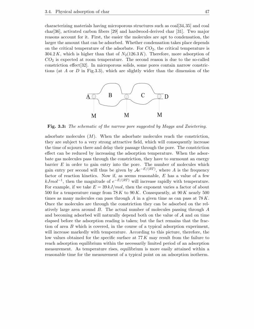
3.4. Physical adsorption of char 47
characterizing materials having microporous structures such as coal[34,35] and coalchar[36], activated carbon fibers [29] and hardwood-derived char [31]. Two majorreasons account for it. First, the easier the molecules are apt to condensation, thelarger the amount that can be adsorbed. Whether condensation takes place dependson the critical temperature of the adsorbate. For CO2, the critical temperature is304.2K, which is higher than that of N2(126.3K). Therefore, more adsorption ofCO2 is expected at room temperature. The second reason is due to the so-calledconstriction effect[32]. In microporous solids, some pores contain narrow constric-tions (at A or D in Fig.3.3), which are slightly wider than the dimension of the
A
M
B
M
C D
MFig. 3.3: The schematic of the narrow pore suggested by Maggs and Zwietering.
adsorbate molecules (M). When the adsorbate molecules reach the constriction,they are subject to a very strong attractive field, which will consequently increasethe time of sojourn there and delay their passage through the pore. The constrictioneffect can be reduced by increasing the adsorption temperature. When the adsor-bate gas molecules pass through the constriction, they have to surmount an energybarrier E in order to gain entry into the pore. The number of molecules whichgain entry per second will thus be given by Ae−E/(RT ), where A is the frequencyfactor of reaction kinetics. Now if, as seems reasonable, E has a value of a fewkJmol−1, then the magnitude of e−E/(RT ) will increase rapidly with temperature.For example, if we take E = 39 kJ/mol, then the exponent varies a factor of about500 for a temperature range from 78K to 90K. Consequently, at 90K nearly 500times as many molecules can pass through A in a given time as can pass at 78K.Once the molecules are through the constriction they can be adsorbed on the rel-atively large area around B. The actual number of molecules passing through Aand becoming adsorbed will naturally depend both on the value of A and on timeelapsed before the adsorption reading is taken; but the fact remains that the frac-tion of area B which is covered, in the course of a typical adsorption experiment,will increase markedly with temperature. According to this picture, therefore, thelow values obtained for the specific surface at 77K may result from the failure toreach adsorption equilibrium within the necessarily limited period of an adsorptionmeasurement. As temperature rises, equilibrium is more easily attained within areasonable time for the measurement of a typical point on an adsorption isotherm.
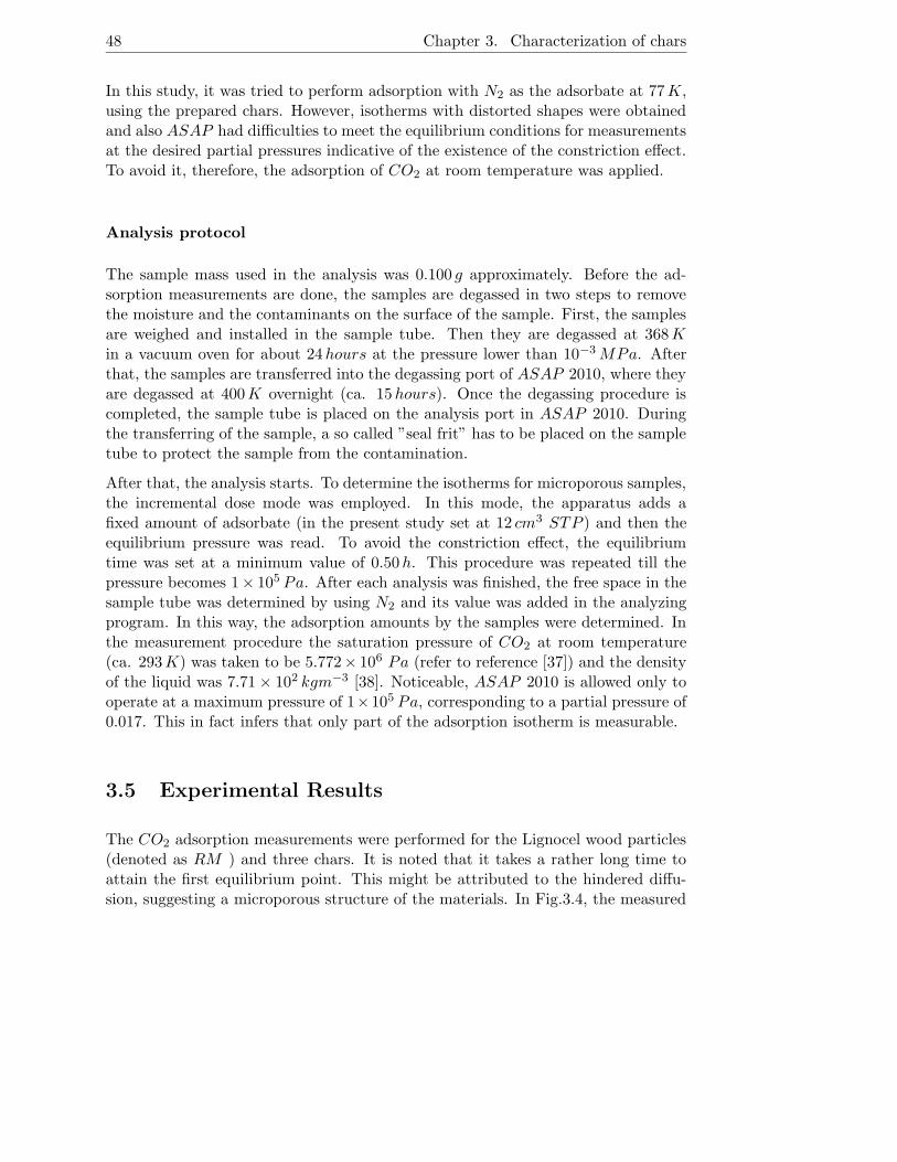
48 Chapter 3. Characterization of chars
In this study, it was tried to perform adsorption with N2 as the adsorbate at 77K,using the prepared chars. However, isotherms with distorted shapes were obtainedand also ASAP had difficulties to meet the equilibrium conditions for measurementsat the desired partial pressures indicative of the existence of the constriction effect.To avoid it, therefore, the adsorption of CO2 at room temperature was applied.
Analysis protocol
The sample mass used in the analysis was 0.100 g approximately. Before the ad-sorption measurements are done, the samples are degassed in two steps to removethe moisture and the contaminants on the surface of the sample. First, the samplesare weighed and installed in the sample tube. Then they are degassed at 368Kin a vacuum oven for about 24hours at the pressure lower than 10−3MPa. Afterthat, the samples are transferred into the degassing port of ASAP 2010, where theyare degassed at 400K overnight (ca. 15hours). Once the degassing procedure iscompleted, the sample tube is placed on the analysis port in ASAP 2010. Duringthe transferring of the sample, a so called ”seal frit” has to be placed on the sampletube to protect the sample from the contamination.
After that, the analysis starts. To determine the isotherms for microporous samples,the incremental dose mode was employed. In this mode, the apparatus adds afixed amount of adsorbate (in the present study set at 12 cm3 STP ) and then theequilibrium pressure was read. To avoid the constriction effect, the equilibriumtime was set at a minimum value of 0.50h. This procedure was repeated till thepressure becomes 1× 10⁵ Pa. After each analysis was finished, the free space in thesample tube was determined by using N2 and its value was added in the analyzingprogram. In this way, the adsorption amounts by the samples were determined. Inthe measurement procedure the saturation pressure of CO2 at room temperature(ca. 293K) was taken to be 5.772× 10⁶ Pa (refer to reference [37]) and the densityof the liquid was 7.71 × 10² kgm−3 [38]. Noticeable, ASAP 2010 is allowed only tooperate at a maximum pressure of 1×10⁵ Pa, corresponding to a partial pressure of0.017. This in fact infers that only part of the adsorption isotherm is measurable.
3.5 Experimental Results
The CO2 adsorption measurements were performed for the Lignocel wood particles(denoted as RM ) and three chars. It is noted that it takes a rather long time toattain the first equilibrium point. This might be attributed to the hindered diffu-sion, suggesting a microporous structure of the materials. In Fig.3.4, the measured

3.6. Theoretical treatment 49
isotherms are given. It is shown that in the measured partial pressure range the Lig-nocel wood only adsorbs little amount of CO2 indicating a low porosity. In contrast,
Fig. 3.4: Calculated and experimental adsorption isotherms of Lignocel wood andthe wood-derived chars.
three chars have relatively large adsorption capacities, which increase at elevatedpyrolyzing temperature of the char. However, this increment tends to be less whenthe pyrolyzing temperature is above 900K. The shape of the measured isothermsresembles type I for microporous material, but the plateau at higher pressures isnot visible due to the restriction of the apparatus in use.
The increment in the adsorption was caused by the newly developed pores in charsduring the pyrolysis. As the pyrolysis temperature increases, more volatiles willevolve from the wood, which leave pores in the residues. When the pyrolyzingtemperature is sufficiently high, the devolatilization process is nearly completed.Then, the increment in adsorption also ceases. The present measurements do notexclude the possibility that the chars have also macropores, as the plateau at higherpressure is not visible. However, the experiments with the standard measurementby using N2 as well as indications from the studies on the adsorption measurementsof chars is considered as a sound basis to assume that the chars are microporous.
3.6 Theoretical treatment
The adsorption of microporous materials has been dealt with by Dubinin [39] usingthe potential theory originally formulated by Polanyi. Prior to the application ofDubinin’s model, the ideas behind it are first briefly reviewed.
Dubinin’s model assumes that the micropores are responsible for adsorption. Astrong attractive potential exists at the pore surface. Because of the strength ofthe potential at the micropore level, the adsorbate condenses during adsorption.

50 Chapter 3. Characterization of chars
The adsorbate fills the volume within the micropores. Only the unoccupied volumeremains available for adsorption. The model is based on characterizing the adsorbentvolume with a reference adsorbate. Once the characteristics of the adsorbent areknown, the predicted volume for a different adsorbate can be determined.
The basic idea is that the adsorption surface in the vicinity of a solid surface is char-acterized by a series of equipotential surfaces. The adsorption potential ε, resultingas it does from the dispersion and polar forces between the solid and the adsorbatemolecules, is independent of temperature but varies according to the nature of theadsorbate as well as that of the solid. According to Dubinin [39], for two differentvapours at the same filling W (volume of condensed adsorbate per mass of adsor-bent), the adsorption potentials will bear a constant ratio to one another no matterwhat the actual value of W is, i.e.
ε
ε0= β. (3.6.1)
The constant ratio β is termed by Dubinin the affinity coefficient. The subscript 0refers to the standard vapour. From thermodynamics, the adsorption potential atconstant temperature, equals the Gibbs’ free energy of adsorption:
ε = RT ln(Ps
P), (3.6.2)
where Ps is the saturated vapour pressure of the adsorbate.
The adsorption can be expressed in a dimensionless form:
θ =W
W∞, (3.6.3)
where W∞ is the filling of the whole adsorption space of pores by the moleculesadsorbed. If we know the relationship between the degree of adsorption θ0 and ε0for the standard vapour (i.e., the characteristic curve), then the relationship betweenθ and ε for any arbitrary adsorbate can be found, since
θ = f(ε0E0
) = f(ε
βE0) = f(
ε
E), (3.6.4)
where E0 is the characteristic adsorption energy of the standard vapour and Eis the characteristc free energy of adsorption of another vapour. Dubinin and hisco-workers argue that the function f may be expressed as a Weibull distribution:
f(ε
E) = exp
[
−(ε
E)n
]
, (3.6.5)
where the exponent n, termed the heterogeneity parameter [40], is a small integer.The value of n, as suggested by Dubinin and Astakov [27], may vary from unity up to

3.6. Theoretical treatment 51
5 or 6. In general it appears that 1 < n < 2 refers to carbon with large micropores.For molecular sieves the value is 2 while very fine pore carbons and zeolites mayrequire values up to 5 or 6. It was also demonstrated that the exponent n decreasesas the surface coverage increases [40].
From Eq. 3.6.5 it follows that at ε = 0 or P = Ps, f = 1; as ε → ∞ or P → 0, thefunction f tends to zero. Therefore, f represents the filled fraction of pores, i.e., θ.Accordingly, the degree of filling of pores can be expressed as
W
W∞= exp
−[
RT
Eln(
Ps
P)
]n
, (3.6.6)
which is named the Dubinin-Astakhov equation. By fitting it to the measuredisotherm, the pore volume W∞ can be determined. E and n are set as the fittingparameters.
A simple approximation equation on calculating the micropore dimension was pro-posed by Dubinin, assuming that the micropores are slit-like. It reads
xE0 = xE/β = k, (3.6.7)
where x is the pore half-width in nm, E in terms of kJmol−1 and the parameterk = 12 kJnmmol−1 is the energy characteristic constant, which was estimated us-ing small-angle x-ray scattering and benzene adsorption data on various activatedcarbons. For the adsorption of CO2 on chars, the affinity β = 0.46 is employed,referring to the literature [30].
In the micropore range, the concept of specific surface area of the chars loses itsvalidity. Due to the strong attractive force field in the vicinity of the surface, theadsorbate molecules no longer distribute in monolayer on the char surface. Instead,they fill the pore. The traditional estimate of specific surface area on the basis ofthe monolayer assumption is then not valid.
The DA equation describes satisfactorily the measured isotherm as depicted in Fig.3.4. In Fig.3.5, an example of a DA plot for the adsorption on Char II is given.It yields straight lines extending over the entire range of relative pressure covered.In Table 3.2 the resulting best-fit values of E, n and W∞ for the adsorption of allsamples are summarized, together with the pore half-width x. As it shows that W∞
of chars is larger than its value for the Lignocel wood and increases with increasingpyrolysis temperature. The adsorption energy E and the heterogeneity factor nfollow the similar trend. But the variance in E and n become less when the pyrolyz-ing temperature is above 800K. In contrast, the pore half-width decreases. Thesefacts indicate that the pyrolyzing temperature merely promotes the creation of newmicropores, which are produced through the devolatilization process. When thisprocess is nearly complete, the development of the micropores accordingly ceases.
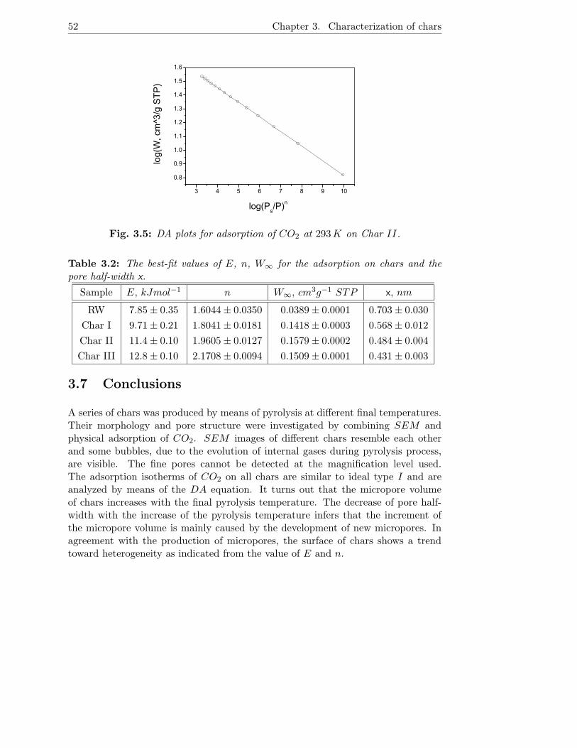
52 Chapter 3. Characterization of chars
Fig. 3.5: DA plots for adsorption of CO2 at 293K on Char II.
Table 3.2: The best-fit values of E, n, W∞ for the adsorption on chars and thepore half-width x.
Sample E, kJmol−1 n W∞, cm3g−1 STP x, nm
RW 7.85 ± 0.35 1.6044 ± 0.0350 0.0389 ± 0.0001 0.703 ± 0.030
Char I 9.71 ± 0.21 1.8041 ± 0.0181 0.1418 ± 0.0003 0.568 ± 0.012
Char II 11.4 ± 0.10 1.9605 ± 0.0127 0.1579 ± 0.0002 0.484 ± 0.004
Char III 12.8 ± 0.10 2.1708 ± 0.0094 0.1509 ± 0.0001 0.431 ± 0.003
3.7 Conclusions
A series of chars was produced by means of pyrolysis at different final temperatures.Their morphology and pore structure were investigated by combining SEM andphysical adsorption of CO2. SEM images of different chars resemble each otherand some bubbles, due to the evolution of internal gases during pyrolysis process,are visible. The fine pores cannot be detected at the magnification level used.The adsorption isotherms of CO2 on all chars are similar to ideal type I and areanalyzed by means of the DA equation. It turns out that the micropore volumeof chars increases with the final pyrolysis temperature. The decrease of pore half-width with the increase of the pyrolysis temperature infers that the increment ofthe micropore volume is mainly caused by the development of new micropores. Inagreement with the production of micropores, the surface of chars shows a trendtoward heterogeneity as indicated from the value of E and n.

Chapter 4
Fast pyrolysis of biomass athigh temperature
4.1 Introduction
Pyrolysis is a thermal degradation process of organic compounds, for biomass exam-ple, in the absence of oxygen, which produces gas, tar and char residues. Dependingon the conditions (heating rate, temperature, particle size etc.) the product distri-bution can be adjusted and optimized. Fast pyrolysis at high temperatures above1000K is of special interest for gasification in fluidized beds since it is the first stepoccurring in the fluidized gasifier. In order to optimize the production of the desiredspecies and also the design of the reactor itself, it is important to understand howthe operating conditions affect the pyrolysis process and what is the kinetics at bothhigh heating rate and high temperature.
Pyrolysis kinetics depends on the heating rate and the residence time of the biomassin the reactor. The main kinetic studies about biomass pyrolysis have been focusedon the thermal decomposition of pure cellulose at low heating rate (< 100K/min)and low temperature range (600K) by TGA. Under such a condition, the pyrolysisof cellulose can be described by a first order global reaction with high activationenergy: 193 kJmol−1 according to Varhegyi et al.[41], Kashiwagi and Nambu[42],Cooley and Antal[43]. This finding was later contradicted by Milosavlijevic [15].He claims that the pyrolysis of the cellulose can be well described by a two-stagemechanism: the first at a low temperature range (T < 667K) with high activationenergy (218 kJmol−1) and the second at a high-temperature range with low activa-tion energy (140 − 155 kJmol−1). Milosavlijevic argued that the examined kineticsis affected by the temperature of the process. A high temperature favors the tarformation pathway in the model proposed by Kilzer and Broido [44] (see Fig. 4.1),
53

54 Chapter 4. Fast pyrolysis of biomass at high temperature
which corresponds to the low activation energy. Miller et al.[45] pointed out that themajority of the pyrolysis occurs at low temperatures due to relatively long exposuretimes required to reach the higher temperatures in TGA; therefore the exclusiveuse of low heating rate TGA experiments can cause difficulties in distinguishing be-tween the high and low temperature contributions to pyrolysis. Later on, Antal [46]suggested that the thermal lag at high heating rate can cause a drop in activationenergy. Till now, there has not been a general agreement as to the global kineticsof the pyrolysis. This leads us to further study the pyrolysis kinetics, especially atboth high heating rates and at a larger temperature range. It is also worth notingthat in most of the studies mentioned above cellulose was used concerning the com-plexity of biomass pyrolytic behavior. Few studies have been done on the pyrolysiskinetics of other materials such as wood. The present chapter mainly deals with thepyrolysis kinetics of Lignocel wood, at high temperature and at high heating rates.
Fig. 4.1: Mechanism of cellulose pyrolysis proposed by Kilzer and Broido [44].
4.2 Pyrolysis characteristics of several biomasses
A great deal of effort has been spent on analyzing the pyrolysis process of Lignocel,because wood is the commonly used material in industrial gasifiers. It is reasonableto assume, at least qualitatively, that the pyrolysis process of wood is closely relatedto the pyrolysis of the three major components, namely cellulose, hemicellulose andlignin. Therefore, the pyrolysis of wood can be represented as the resultant of thepyrolysis of the individual components. This may form a sort of tool in character-izing the chemical composition of the wood, which also helps the understanding ofits overall pyrolysis performance.
The pyrolysis of cellulose, lignin and Lignocel wood were characterized by usingTGA. Following the aforementioned experimental procedure (see section 2.3), thepyrolysis was carried out at a final temperature of 1273K and at several heatingrates: 20Kmin−1, 40Kmin−1 and 60Kmin−1. The curves of weight loss versustemperature (called TGA curves) are plotted for three materials in Fig. 4.2(a). Theheating rate of this series of experiments is 20Kmin−1. Three stages can be ob-served. In stage I, a slight weight loss occurred due to the elimination of moisture
4.2. Pyrolysis characteristics of several biomasses 55
present in raw material, which is also called dehydration. Subsequently, the biomassdid undergo the essential process, i.e. devolatilization of biomass, during which mostof the volatiles are released. In the third stage, there existed a slow decompositionof the solid residue. During this process, its structure gradually approaches thatof graphite by means of crystalline re-orientation. This stage is termed carboniza-tion. By taking the time derivative of the TGA curves (d(m/m0)/dt), the effectof the temperature on the pyrolysis can be more clearly seen from these so-calledDTG curves as shown in Fig. 4.2(b). The temperature range corresponding to the
(a) TGA curve (b) DTG curve
Fig. 4.2: Pyrolysis of cellulose, lignin and Lignocel at the heating rate of 20Kmin−1
in the TGA.
devolatilization is different for the three materials. For the convenience of compari-son, the onset temperature of the devolatilization is denoted as Ti; the terminationtemperature of this stage is Te. The temperature that corresponds to the maximumdevolatilization rate is defined as Tm. The determination of both Ti and Te is basedon an empirical extrapolation method as depicted in Fig. 4.3. The onset tempera-
Fig. 4.3: Determination of onset temperature and the termination temperature ofdevolatilization.

56 Chapter 4. Fast pyrolysis of biomass at high temperature
ture is the temperature at the position of point D, which is the intersection point ofthe tangent (drawn at the point of maximum slope of the leading edge (AB) of thepeak), and the extrapolated base line (AD). A and D represent points where thecurve begins to deviate from the base line. The same method holds for the determi-nation of Te as well. This extrapolation was done by using the associated software“TGA instrument universal analysis 2000”. The determined values of Ti, Tm and Te
are summarized in Table 4.1. Cellulose pyrolyses over a narrow temperature rangeof 567K-663K. This is consistent with the narrow range of chemical bond types incellulose, which decompose in a small temperature range. In contrast to cellulose,the pyrolysis of lignin exhibits a gradual weight loss over a larger temperature range.This is attributed to the wide variety of bond strengths present in the lignin. TheDTG curve of Lignocel wood is not as symmetric as that of cellulose. At 570K, theleft side of the curve shows a shoulder peak. It might be caused by the decomposi-tion of the hemicellulose in the wood. Unfortunately, it was not possible to collect
Table 4.1: Comparison of the temperature characteristics of devolatilization ofcellulose, lignin and Lignocel wood at the heating rate of 20Kmin−1.
Sample Ti,K Tm,K Te,K
Cellulose 567 624 663
Lignin 444 630 771
Lignocel wood 496 636 673
a sample of hemicellulose due to some technical limitations. However, with the aidof the literature, it is possible to verify this hypothesis. Sørensen[47] has comparedthe pyrolysis of three components which were derived from sources different fromthe present materials at a heating rate of 5Kmin−1. He proved that hemicellulose(extracted from Spruce) is the least stable component with respect to cellulose andlignin. Its main decomposition occurs in the temperature range of 473K-573K andpeaks at 523K. He mentioned that at a heating rate of 40Kmin−1, the tem-perature range may shift to a higher temperature by 50K. Therefore, the Tm forhemicellulose decomposition is in between 523K-573K. This reasonably fits thepeak temperature of the shoulder. In the high temperature region of the DTGcurve of Lignocel wood, there is a rather flat tail, which is merely caused by thedecomposition of lignin. Considering that the pyrolysis of wood can be representedas the combination of the pyrolysis of the individual components, the main pyrolysisrate of wood can be described according to a superposition model [48, 49],
[
(d(X)
dt)|T
]
w
=
[
(d(X)
dt)|T
]
c
× ωc +
[
(d(X)
dt)|T
]
l
× ωl
+
[
(d(X)
dt)|T
]
h
× ωh, (4.2.1)

4.2. Pyrolysis characteristics of several biomasses 57
where ω is the weight percentage, the subscripts w, c, l and h represent wood,cellulose, lignin and hemicellulose respectively. The first two terms on the right-hand side of Eq. 4.2.1 are directly obtained from the individual DTG curves. Theconversion X is given by
X =m0,i −mi
m0,i −mchar,i, (4.2.2)
where i refers to wood and other three components. Because lack of data on thepyrolysis of hemicellulose, the pyrolysis rate of wood can only be partially superim-posed. As mentioned before, the hemicellulose decomposes in a temperature rangeof 523-573K. Therefore, above 573K the decomposition of the Lignocel can beconsidered as a combination of the decomposition of cellulose and lignin. Sincethe maximum decomposition rates dX/dt of the cellulose and the lignin take placeabove 573K, the superimposed maximum decomposition rate dX/dt must equal theobserved one.
The difference between the experimental and the superimposed DTG curves is givenas the percentage of the highest measured dX/dt value:
Dev1 = 100% ×√
SDTG/(Z −N)
max[(−dX/dt)exp], (4.2.3)
where SDTG is the sum of the squared residuals, Z is the number of data points andN is the number of parameters employed in Eq. 4.2.1. In Fig. 4.4 the superposedDTG curve is presented together with the experimental one. The mass fractionsof the cellulose and the lignin are found to be 32% and 25% with a deviation ofDev1 = 0.114. In comparison with the DTG curve of the Lignocel wood, the
Fig. 4.4: DTG curves of the Lignocel wood and the superposition of the pyrolysisof cellulose and lignin. The heating rate is 20Kmin−1.
temperature at the maximum pyrolysis rate in the superimposed DTG curve isabout 10K lower. This deviation may have several causes. The first one is the

58 Chapter 4. Fast pyrolysis of biomass at high temperature
catalytic effect of ash in Lignocel wood (refer to Table 2.1). Besides the catalyticeffect, the used cellulose and lignin may also have different crystallinities from thosepresent in Lignocel wood. The estimated mass fractions of cellulose and ligninare 32% and 25%, respectively. The rest consists of hemicellulose, extractablesand ashes. The above superposition provides a qualitative insight in the chemicalstructure of Lignocel wood and its apparent pyrolysis characteristics.
The product distribution of pyrolysis is a complex function of the conditions such astemperature, heating rate as well as the chemical composition of the material. Py-rolysis experiments were performed at the heating rates of 20Kmin−1, 40Kmin−1
and 60Kmin−1, respectively. The yields of moisture, volatile, char and ash arederived and listed in Table 4.2.
Table 4.2: The yields of moisture, volatile, char and ash (%).
Sample Heating rate,Kmin−1 Moisture Volatile Char Ash
20 2.558 81.51 12.81 3.115
Lignocel 40 2.138 81.93 13.02 2.910
60 2.709 80.85 12.92 3.386
20 2.584 95.58 1.836 −Cellulose 40 2.189 95.94 1.871 −
60 2.885 95.21 1.902 −20 1.233 64.76 34.01 −
Lignin 40 0.894 65.91 33.37 −60 1.447 65.14 33.41 −
No influences of heating rates were found on the product distribution for all materi-als. Pyrolysis of cellulose mainly gives rise to volatiles and in contrast, lignin is themain origin for char production due to its aromatic structure. This again confirmsthat the Lignocel wood mainly consists of cellulose and some amount of lignin asindicated from the product distribution.
4.3 High temperature pyrolysis in a shock tube reactor
The preceding section provides some fundamental aspects of the chemical structureof the Lignocel wood and its pyrolysis behavior at low heating rate (< 100Kmin−1).Continuing this study, the pyrolysis of Lignocel wood at a high temperature range(950K-1500K) and a high heating rate (O(103)Kmin−1) will be investigated bymeans of the shock tube reactor. The keynote is to find the kinetics parameters

4.3. High temperature pyrolysis in a shock tube reactor 59
including the activation energy and the reaction order via the extinction technique(see section 2.5.3), which requires a constant number density of particles in theobservation region. To begin with, the trajectories of the wood particles during thepyrolysis are studied in section 4.3.1. Subsequently, the heat transfer involved inpyrolysis will be estimated in section 4.3.2. On this basis, the kinetics parametersof the pyrolysis will be calculated.
4.3.1 Trajectories of wood particles in the shock tube
The observation window is located at 0.075m away from the end plate of the shocktube. There, the pyrolysis of the particle is measured by the extinction techniqueas described in Chapter 2. The change of the transmitted light intensity may becaused by two phenomena. In the first case, particles shrink when reaction occurs.The other possibility is that the motion of the particles crossing the observationregion induces a variation of the particle density. To ascertain which phenomenonis dominant, the trajectories of the particles will be first investigated.
Theory
The particles are accelerated by the moving gas behind the incident shock andare decelerated by the stagnant gas behind the reflected shock. The trajectorycalculation will therefore be performed in two steps.
As a quick start, a simple estimate is performed to predict the trajectory of theparticles behind the reflected shock. In Fig. 4.5 the position of the particles beforethe passage of the incident shock and after that of the reflected shock are depicted.The distance of the right front of the suspension to the end plate is xinj initially
-
-
XinjXM
Suspensionfront
Suspensionfront
Endplate
Fig. 4.5: The distances of the suspension front to the end plate.
and is xM after the passage of the reflected shock. The mass conservation of the gasin between the front and the end plate yields
ρ1xinj = ρ5xM . (4.3.1)
Rearranging it givesxM
xinj=ρ1
ρ5. (4.3.2)

60 Chapter 4. Fast pyrolysis of biomass at high temperature
2.2 2.4 2.6 2.8 3 3.2 3.4 3.6 3.8 40.06
0.07
0.08
0.09
0.1
0.11
0.12
0.13
0.14
Ms1
x M/x
inj
2.2 2.4 2.6 2.8 3 3.2 3.4 3.6 3.8 40
10
20
30
40
50
60
70
80
90
100
P4/
P1
Fig. 4.6: The relative position xM/xinj ofthe particle with respect to the shock Machnumber Ms1 and the pressure ratio P4/P1.
2.2 2.4 2.6 2.8 3 3.2 3.4 3.6 3.8 40.4
0.6
0.8
1
1.2
1.4
Ms1
x inj
, m
2.2 2.4 2.6 2.8 3 3.2 3.4 3.6 3.8 40
1
2
3
4
5
6
7
8
9
10x 10
4
P1,
Pa
Fig. 4.7: The required position xinj withrespect to the shock Mach number Ms1 andthe initial pressure of the test gas P1 as-suming xM = 0.075m.
The subscripts 1 and 5 refer to regions 1 and 5 as shown in Fig. 2.20 and the sameholds for the rest of this section. The density ratio ρ1/ρ5 is derived from the shocktube theory referring to Eq. 2.5.6. It is a function of the shock Mach number Ms1
that depends on the incident shock velocity. Via the shock Mach number Ms1, thepressure ratio P4/P1 can also be correlated to the relative position xM/xinj . In Fig.4.6 the ratio of xM/xinj is plotted against the shock Mach number Ms1 and P4/P1.It is seen that the larger the pressure ratio is, the higher the shock Mach numberis and the closer the particle will be to the end plate. With this graph we can tellwhere the initial suspension front should be and what initial pressure of the testgas should be selected, given the location of the observation window. In Fig. 4.7the relation of xinj , P1 and Ms1 is illustrated. The observation window is 0.075maway from the end plate. Suppose that P1 ranges from 150mbar to 300mbar, thesuspension front needs to be at a distance of 0.9 − 1m from the end plate for aconstant driver gas pressure of 11 bar.
The above estimate indicates that the pressure ratio P4/P1 and the position ofthe suspension could influence the location of the particles after the passage ofthe reflected shock. To observe the pyrolysis of the particle at this location mayrequire specific experimental conditions, for example a specific pressure ratio. Inthe following a more detailed calculation is done with regard to the acceleration andthe deceleration of the particles.
Acceleration behind the incident shock When the incident shock front reachesthe particles, the particle will be accelerated by the moving gas behind the shock.

4.3. High temperature pyrolysis in a shock tube reactor 61
The drag force on the cylindrical particle reads, according to [26],
Fb =1
2Cb2ρ2U
2Ap, (4.3.3)
where Ap is the frontal area of the cylinder, namely, Ap = HpDp, if Hp is the lengthof the cylinder. U = u2 − up2 is the velocity of the gas stream relative to theparticle. Cb2 is the drag coefficient, which is dependent on the value of the Reynoldsnumber Re = UD/ν. Here we consider a single smooth cylinder in cross-flow andthe relationship between Cb2 and Re number is given by [26]:
Cb2 = B1ReB2 , (4.3.4)
where B1 = 10.52 and B2 = −0.6132 for a single smooth cylinder in cross-flow. Ac-cording to Newton’s second law, the acceleration of the particle, a can be expressedas
a =Fb
mp. (4.3.5)
Combining Eqns. 4.3.3-4.3.5 leads to
a = C2U(2+B2), (4.3.6)
with
C2 =ρ2ApB1D
B2p
2mpνB22
. (4.3.7)
The acceleration a is also defined as the time derivative of the particle velocitydup2/dt. This results in
a =dup2
dt= C2U
(2+B2),
= C2(u2 − up2)(2+B2). (4.3.8)
The initial condition for this differential equation is up2 = 0 at t = 0, which meansthat the particle is stagnant when the shock reaches it. Solving Eq. (4.3.8) withthis boundary condition yields
up2(t) = u2 −[
u−(1+B2)2 + (1 +B2)C2t
]−1
1+B2 . (4.3.9)
Integrating Eq.(4.3.9) gives the displacement of the particle as a function of time,
x2(t) = u2t−1
B2C2
[
u−(1+B2)2 + (1 +B2)C2t
]
B21+B2 − u−B2
2
. (4.3.10)

62 Chapter 4. Fast pyrolysis of biomass at high temperature
With Eq. (4.3.10) the trajectory of the particle behind the incident shock can becalculated. It is valid as long as the particle is behind the incident shock. Accordingto Eq. (4.3.10), the acceleration of the particle has a characteristic time of
τc2 =1
(1 +B2)C2u(1+B2)2
. (4.3.11)
The reflected shock When the particle reaches the reflected compression shock itwill be decelerated by the stagnant gas behind the shock. To model the trajectory weneed to know at which time, ts, the reflected compression shock meets the particle.At t = ts, the particle has a displacement of
xs(ts) = u2ts −1
B2C2
[
u−(1+B2)2 + (1 +B2)C2ts
]
B21+B2 − u−B2
2
. (4.3.12)
At time ts the incident shock has travelled from the injection point to the end plateand reflected from the end plate to a distance xr towards the front plate as depictedin Fig.4.8. Since the velocities of both the incident shock and the reflected shock
- -
Displacement ofthe particle xs at t = ts
0
(Injection point)
Displacement ofthe reflected shock xr
xinj
(End plate)
Fig. 4.8: Displacements of the particle and the reflected compression shock at t = ts.
are known, the distance xr can be calculated as
xr(ts) = Us5(ts −xinj
Us1). (4.3.13)
Here xinj is the distance between the injection point and the end plate, Us1 andUs5 are the velocities of the incident shock and the reflected shock, respectively.Therefore, the displacement of the particle xs can be expressed in terms of theshock speeds:
xs(ts) = xinj − xr,
= xinj − Us5(ts −xinj
Us1). (4.3.14)
Combining Eqns. (4.3.12) and (4.3.14) gives the solution to ts.

4.3. High temperature pyrolysis in a shock tube reactor 63
Deceleration behind the reflected shock Following the same reasoning asbefore, the deceleration of the particle behind the reflected shock can be calculatedas
a =Fb
mp= −Cb5u
(2+B2)p5 . (4.3.15)
Here, up5 is the velocity of particle behind the reflected shock. The drag coefficientCb5 follows from:
Cb5 = B1ReB2 . (4.3.16)
Applying the relation a = dup/dt leads to
dup5
dt= −C5u
(2+B2)p5 . (4.3.17)
with
C5 =ρ5ApB1D
B2p
2mpνB25
. (4.3.18)
Integrating Eq. 4.3.17 with the boundary condition up5(ts) = up2 gives the particlevelocity
up5 =[
(1 +B2)C5(t− ts) + up2ts−(1+B2)
]−1
1+B2 . (4.3.19)
Thus, the displacement of the particle x5 can be obtained by integrating Eq. (4.3.19)in t. The particle displacement x5 is expressed as
x5(t) =1
B2C5
[
(1 +B2)C5(t− ts) + up2(ts)−(1+B2)
]
B21+B2 +
up2(ts)−B2
B2C5+ x2(ts).
(4.3.20)The corresponding characteristic time for deceleration is then
τc5 =1
(1 +B2)C5up2(ts)(1+B2). (4.3.21)
By comparing the two characteristic times τc2 and τc5, we know which one is theprevailing process to determine the final location of the particle in the shock tube.The ratio τc5/τc2 is formulated as follows:
τc5τc2
=ρ2
ρ5
(
ν5
ν2
)B2(
u2
up2
)(1+B2)
. (4.3.22)
Now, the complete trajectory of the particle can be calculated by combining Eqns.(4.3.10) and (4.3.20). In Fig. 4.9 a trajectory of a particle injected at 0.7m from theend plate is shown. Such a particle will reach the observation window at 0.075mfrom the end plate. In practice, injection occurs at S = 1.45m. Experiments in

64 Chapter 4. Fast pyrolysis of biomass at high temperature
0 0.1 0.2 0.3 0.4 0.5 0.60
0.5
1
1.5
2
2.5
3x 10
−3
distance to end plate, m
time,
strajectory
incident shock
reflected shock
Fig. 4.9: Trajectory of a wood particle at Us1 = 1050ms−1.
a glass tube have shown that particles are dispersed over a distance of 1m withrespect to S. The particle velocity and the corresponding Reynolds number are alsoshown in Figs. 4.10(a) and 4.10(b), respectively. It clearly shows the accelerationand the deceleration of the particle. The deceleration is faster than the accelerationat given conditions.
0 0.5 1 1.5 2 2.5 3
x 10−3
−100
0
100
200
300
400
500
600
700
800
900
1000
time, s
u p, m
s−1
(a)
0 0.5 1 1.5 2 2.5 3
x 10−3
0
20
40
60
80
100
120
140
160
180
200
time, s
Re
(b)
Fig. 4.10: The particle velocity and the relative particle Reynolds number as afunction of time.

4.3. High temperature pyrolysis in a shock tube reactor 65
Results
From the above considerations it follows that several variables affect the trajectory ofthe particle. They are the particle size, the density of the particle, the initial positionof the particle, the initial gas density and the incident shock speed determined bythe initial pressure ratio between the test gas and the driver gas. In the shocktube experiment, small Lignocel wood particles were selected by using a fluidizedbed. The SEM characterization shows that the particles are not homogenouslydistributed, but the majority of the particles has the dimension of Dp = 10µm andHp = 50µm. Considering the heterogeneous size distribution of the wood particles,we focus on the influence of the particle size and the incident shock velocity onthe trajectory. The initial position of the particle is at xinj = 0.692m. Incidentshock speeds of 850ms−1 and 1050ms−1 are chosen. They correspond to stagnantgas temperatures of 990K and 1400K, respectively. Several quantities are usedto estimate the influence: the ratio of the characteristic deceleration time to thecharacteristic acceleration time τc5/τc2. Basically, if τc5/τc2 is much less than unity,the deceleration of particles is less important than the acceleration. If τc5 is shortwith respect to the pyrolysis time, the particles are stagnant when reaction takesplace and the number density of particles is constant in the observation region. As aresult, the change of the transmission in Fig. 2.26 is solely related to the decreasingparticle size due to the decomposition of particles referring to Eq. 2.5.31.
In Fig. 4.11, the effect of the particle size on the trajectory is displayed for particlediameters: Dp = 5µm, 10µm, 20µm, 30µm. The acceleration of all particles arepresumed to start at 0.692m to the end plate. For large particle, the decelerationstarts at relatively farther distance to the end plate, but needs longer decelerationtime to become stagnant. Within the test time of the shock tube 4ms, large particle
0 0.1 0.2 0.3 0.4 0.5 0.60
0.5
1
1.5
2
2.5
3x 10
−3
distance to end plate, m
time,
s
trajectory
incident shock
reflected shock
Dp=
20 µ
m
Dp=
5 µ
m
Fig. 4.11: The effect of particle size on the trajectory when Us1 = 1050ms−1.

66 Chapter 4. Fast pyrolysis of biomass at high temperature
can not reach the observation window. In contrast, the particle with Dp = 5µmjust passes the observation window during the acceleration and starts deceleratingat a relatively high speed. Only the particle whose size is in a narrow range aroundDp = 10µm can stay in the observation region. In this case, the number density ofthe particle is constant in the observation region. This conclusion only holds for thecase that all the particles started the acceleration at the same position. In reality,there exists a particle size distribution after the injection. Due to the injection,small particles travel to a distance near the end plate and large particles either dropdown or stay near the injection position. In this case, one can imagine that it willbecome far more difficult for the large particles to reach the observation region.Only those small particles with a narrow range of particle sizes can stay stagnantand be observed.
To further confirm the above observation, the ratio τc5/τc2 and the characteristicdeceleration time τc5 were computed for different particle sizes and different incidentshock velocities. The results are listed in Table 4.3. The deceleration time should be
Table 4.3: The influence the particle diameter Dp on the trajectory.
Us1 = 850ms−1 Us1 = 1050ms−1
Dp, µm τc5/τc2 τc5, ms Dp, µm τc5/τc2 tc5, ms
5 0.5831 0.020 5 0.5418 0.018
10 0.5835 0.062 10 0.5424 0.055
20 0.5887 0.190 20 0.5493 0.171
30 0.6020 0.374 30 0.5657 0.340
sufficiently short because the motion of the particle in the observation window willlead to a time dependent number density of the particles. The resulting decelerationtime is much shorter than the acceleration time. With an increase of the incidentshock velocity, the deceleration time tends to be shorter. For a particle with Dp ∼10µm, the deceleration time ranges from 0.055-0.062ms in the temperature rangeof interest. It is noted that the deceleration time refers to the moment a particlemeets the reflected shock. If the deceleration time is of the same magnitude as thetime constant of the transmission signal, the change of the light transmitted signalshould be attributed to both the motion of particle and the reaction.
4.3.2 Heat transfer assessment
The heat exchange between particles and gas appears very crucial in determiningthe pyrolysis kinetics of biomass. With the existence of a temperature variationwithin the biomass particle and of a gap between the ambient gas temperature

4.3. High temperature pyrolysis in a shock tube reactor 67
and the particle temperature, one can imagine that the pyrolysis will take place ina non-uniform manner inside the particle. Using the ambient temperature and theempirical Arrhenius reaction mechanism will then obviously lead to an erroneous in-terpretation of pyrolysis kinetics. The preferred condition is an isothermal pyrolysis,which means that the temperature inside the particle is homogeneous. In fact, twoheat transfer processes and one chemical reaction are competing: the heat transferfrom the ambient gas to the particle surface, the heat transfer needed for the heat-upof the entire particle and the pyrolysis. Three characteristic times corresponding tothe above three processes are defined as τ1, τ2 and τ3.
Let us consider a particle subjected to a sudden temperature change. First, thesurface temperature of the particle will be affected and the temperature disturbancewill diffuse into the particle. A characteristic time for a radial heat diffusion in acylindrical particle, indicating when the temperature differences within the particledisappear, is given by [50]:
τ2 =1
αpa2n
, (4.3.23)
where the characteristic values an are the roots of a Bessel’s equation of order zero:
J0(anDp
2) = 0, (4.3.24)
in which Dp is the diameter of the particle. In the following calculation, the firstpositive root a1 is used.
If we may assume that the temperature difference within the particle is sufficientlysmall, the time dependent particle temperature satisfies:
ρpVpcp∂Tp
∂t= hg(Tg − Tp)S, (4.3.25)
where the surface-averaged heat transfer coefficient hg reads
hg =kgNuL
L . (4.3.26)
If we consider the particle as a spheroid characterized by two dimensions (C, B),the universal correlation of NuL developed by Yovanovich[26] is:
NuL = Nu0L +
[
0.15
(PL
)0.5
Re0.5L + 0.35Re0.566
L
]
Pr1/3. (4.3.27)
It is recommended for 0 < ReL < 2 × 10⁵, Pr ≥ 0.7, and 0 < C/B < 5. Theparameter P in Eq. 4.3.27 is the maximum (equatorial) perimeter of the spheroid,
perpendicular to the flow direction. The constant Nu0L is the overall Nusselt number

68 Chapter 4. Fast pyrolysis of biomass at high temperature
in the pure conduction limit. The Reynolds number Re in Eq. 4.3.27 is a functionof the relative particle velocity:
ReL =|up − ug|L
νg, (4.3.28)
where L is the square root of the spheroid surface. As shown in Fig. 4.10(b), Reis also changing with time. Therefore, Eq. 4.3.25 has to be solved numerically bycombining Eqns. 4.3.9 and 4.3.19. In Fig. 4.12 a two-step heating of the particleis illustrated. First, the particle was heated up to a temperature Tm, ranging from
0 0.5 1 1.5 2 2.5 3 3.5 4
x 10−3
400
600
800
1000
1200
1400
time, s
T p, K
Fig. 4.12: The particle temperature profile(—) obtained as to different gastemperatures(−−−).
600K to 800K, by the gas behind the incident shock. Subsequently, it was heatedonce more by the gas behind the reflected shock to the stagnant gas temperature Tg.If the characteristic time for the particle reaching the gas temperature is defined as
τ1 = t(Tp = 0.9 ∗ (Tg − Tm)) − t(Tp = Tm), (4.3.29)
a characteristic heat-up time τ1 = 0.36ms was obtained, which is independent ofthe chosen gas temperature range.
Negligible intra-particle temperature difference requires the prerequisite of τ2 τ1. When it is satisfied, the external heat transfer is the dominating heat transfermechanism. If the reaction time τ3 is longer than the heat diffusion time τ1, thepyrolysis takes place at stagnant gas temperature. If τ2 < τ3 < τ1, the pyrolysisoccurs simultaneously with the temperature increases. Of course, in any case, thereaction time τ3 shall be shorter than the test time of the shock tube, i.e., ttest =4ms. In Fig. 4.13, the characteristic times: τ1 and τ2 as functions of the particle

4.3. High temperature pyrolysis in a shock tube reactor 69
size are depicted. First of all, it is found that the heat penetration time τ2 is smallerthan τ1 for Dp < 55µm. For Dp < 55µm, a chemically controlled regime (abcd)is found if τ1 < τ3 < ttest is satisfied. For Dp = 10µm, a chemically controlledpyrolysis requires a reaction time larger than 0.36ms. Further, it is realized thatit is very difficult to extract information on the kinetics if the reaction time is lessthan 0.065ms.
Fig. 4.13: The characteristic times versus different particle sizes.
4.3.3 Kinetics assessment
The pyrolysis rate of the biomass can generally be represented by
dXdt
= A exp(−ERTp
)(1 −X )n, (4.3.30)
where X is the conversion, Tp the particle temperature, A the frequency factor, Ethe activation energy, n the reaction order and R the gas constant.
Three cases have to be considered: τ3 > τ1 > τ2, τ1 > τ3 > τ2 and τ2 > τ3. Thefirst two cases can be analyzed in the same way if only data collected later than theheat-up time (after the arrival of the reflected shock) will be analyzed. After theheat-up time the particle temperature may be taken constant and equal to the gastemperature. In Chapter 2, we have shown that the particle temperature is lowerthan the gas temperature due to the radiation heat transfer. The temperaturedifference depends on the particle dimension. Because of the changing particle sizeand the uncertainties in the calculation of the gas temperatures, we did not takethe temperature difference into account. Under this condition, Eq. 4.3.30 can bereduced to
dXdt
= A′(1 −X )n, (4.3.31)

70 Chapter 4. Fast pyrolysis of biomass at high temperature
where the constant A′ = A exp(−E/(RTg)). Integrating it for n = 1 and n 6= 1yields
n = 1 X = 1 − exp(−A′t), (4.3.32)
n 6= 1 X = 1 −[
1 + (n− 1)A′t] 1
1−n . (4.3.33)
Eq. 4.3.33 is used to retrieve A, E and n, The fitting procedure is performed intwo steps by using the package nlinfit in Matlab. First, the best-fit values of A′ andn with the highest value of R2 can be determined for the pyrolysis experiments inthe temperature range of 950K-1500K. Since A′ = A exp[−E/(RTg)], lnA′ versusTg will follow a linear relationship if the pyrolysis takes place in the chemicallycontrolled regime. Further, according to Eq. 4.3.33, the characteristic reaction timeis
τ3 =1
(n− 1)A′. (4.3.34)
By comparing τ3 with τ1, one can identify whether the obtained kinetics parameterscorresponds to the chemically controlled pyrolysis.
In this analysis, the conversion X is defined as follows:
X =m0 −m(t)
m0 −mres,
=ρpπD
2p0Hp0 − ρpπDp(t)
2Hp
ρpπD2p0Hp0 − ρpπD2
p,resHp,
=D2
p0Hp0 −Dp(t)2Hp
D2p0Hp0 −D2
p,resHp, if ρp is constant, (4.3.35)
where Dp0 represents the initial particle radius when no reaction occurs and Dp,res
is the particle radius of the char residue. Assuming that the shrinking of particlemerely takes place radially, then the above equation can be approximated as
X =1 − (Dp(t)/Dp0)
2
1 − (Dp,res/Dp0)2. (4.3.36)
We have derived in Chapter 2 that the particle size Dp is related to the transmittedintensity according to Eq. 2.5.31:
I = I0 exp(−CDp). (4.3.37)
If the number density of particles Np is constant, the conversion X can now berelated to the light intensity as
X =1 −
(
ln(I(t)/I0)ln(Ires/I0)
)2
1 −(
ln(I(b)/I0)ln(Ires/I0)
)2 , (4.3.38)

4.3. High temperature pyrolysis in a shock tube reactor 71
where I(b)/I0 corresponds to the lowest transmission in Fig. 2.26 and Ires/I0 cor-responds to the transmission when the reaction is completed.
4.3.4 Experimental results
The pyrolysis of Lignocel wood was performed in a gas temperature range 950K-1500K. Firstly, the influence of the particle motion on the transmission signalwas investigated. In Fig. 4.14(a) the measured pressure and transmission at Tg =970K near the end plate are shown. The zone where the particle motion willprobably interfere with the reaction is shaded and zoomed in in Fig. 4.14(b). Itclearly shows that the transmission decreases to position b after the passage of
(a) (b)
Fig. 4.14: The history of pressure and transmission near the end plate. Tg = 970K.
the reflected shock. Subsequently, it becomes constant in a narrow time periodof 0.07ms, which indicated no occurrence of either reaction or the motion of theparticle. According to Table 4.3, the deceleration time decreases with the increase ofthe incident shock velocity (gas temperature). We expect, therefore, that no effectof particle motion will occur at elevated temperatures. It is noted that, during theconstant time period [b, c], a gradual increase of the pressure was observed, whichindicates a gradual increase of the gas temperature. After that, the pressure (or thegas temperature) becomes constant and the transmission begins to increase becausethe reaction takes place. The pyrolysis conversion defined by Eq. 4.3.38 is displayedin Fig. 4.15. In agreement with the transmission curve, the conversion is zero in theinitial narrow region and rapidly increases subsequently. Because the particle motionis affected by the incident shock velocity, the pressure and transmission signalsobtained at Tg = 1190K were also studied. In Fig. 4.16, only part of the pressureand transmission signals are given. No plateau is found near the minimum of thetransmission signal. But, the pyrolysis already starts before the gas approaches the
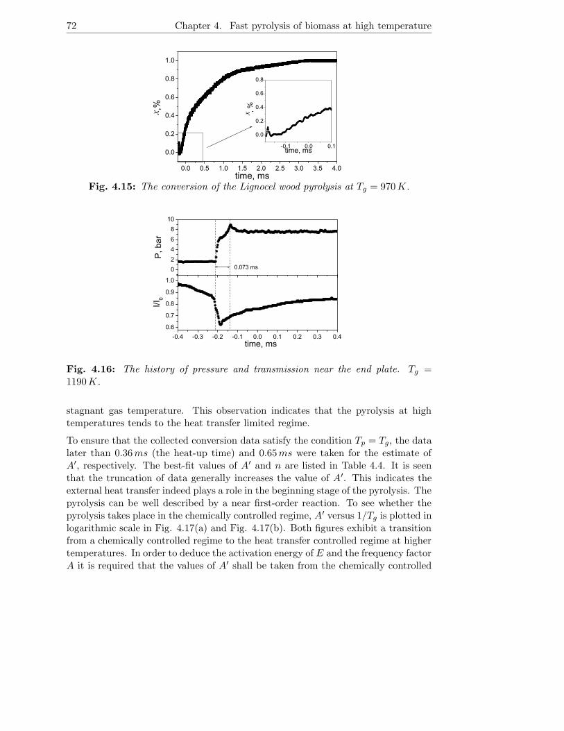
72 Chapter 4. Fast pyrolysis of biomass at high temperature
Fig. 4.15: The conversion of the Lignocel wood pyrolysis at Tg = 970K.
Fig. 4.16: The history of pressure and transmission near the end plate. Tg =1190K.
stagnant gas temperature. This observation indicates that the pyrolysis at hightemperatures tends to the heat transfer limited regime.
To ensure that the collected conversion data satisfy the condition Tp = Tg, the datalater than 0.36ms (the heat-up time) and 0.65ms were taken for the estimate ofA′, respectively. The best-fit values of A′ and n are listed in Table 4.4. It is seenthat the truncation of data generally increases the value of A′. This indicates theexternal heat transfer indeed plays a role in the beginning stage of the pyrolysis. Thepyrolysis can be well described by a near first-order reaction. To see whether thepyrolysis takes place in the chemically controlled regime, A′ versus 1/Tg is plotted inlogarithmic scale in Fig. 4.17(a) and Fig. 4.17(b). Both figures exhibit a transitionfrom a chemically controlled regime to the heat transfer controlled regime at highertemperatures. In order to deduce the activation energy of E and the frequency factorA it is required that the values of A′ shall be taken from the chemically controlled

4.3. High temperature pyrolysis in a shock tube reactor 73
Table 4.4: The best-fit values of A′ and n.
4t = 0.36ms 4t = 0.65ms
Tg, K n A′, s−1 R2 Tg, K n A′, s−1 R2
970 1.298 2534.4 0.943 970 1.234 2016.3 0.9937
980 - - - 980 1.298 2534.4 0.9430
1010 1.069 2744.6 0.9824 1010 1.3035 3126.3 0.9679
1050 1.101 2436.8 0.9982 1050 1.3093 3831.4 0.9823
1050 1.343 9000 0.9188 1050 1.069 7600 0.9000
1110 1.206 9500 0.9483 1110 1.152 10800 0.8965
1190 1.243 7799.9 0.9901 1190 1.325 9000 0.9763
1220 1.065 8000 0.9420 1220 1.220 9999.8 0.9892
1260 1.400 12200 0.9873 1260 1.343 14200 0.9828
1400 1.225 11000 0.9888 1400 1.267 12000 0.9915
regime. Using Eq. 4.3.34, the characteristic reaction times were calculated as to
(a) Conversion data collected after 0.36 ms (b) Conversion data collected after 0.65 ms
Fig. 4.17: Plots of A′ versus 1/Tg.
various gas temperatures. Combining these data with the data in Fig. 4.13, theexperiments which take place in the chemically controlled regime can be selectedas shown in Fig. 4.18. It clearly shows that the pyrolysis below 1220K is in thechemically controlled regime. The obtained A′ below 1220K can then be used tocalculate E and A. In Fig. 4.18 the corresponding Arrhenius plot is presented. Thevalues of E = 106 ± 18.5 kJmol−1 and A = (9.8 ± 2.3) × 108 s−1 are found.

74 Chapter 4. Fast pyrolysis of biomass at high temperature
Fig. 4.18: The diagram of the character-istics times versus the particle diameters.• the experimentally determined charac-teristic reaction times.
Fig. 4.19: The Arrhenius plot (in loga-rithmic scale) for the pyrolysis of Ligno-cel wood in the gas temperature range of950K-1200K.
In comparison to the literature reported activation energies, the present result isgenerally lower than those obtained by TGA. Intra-particle heat transfer and exter-nal heat transfer have been excluded in the assessment of the kinetics. We believethat the relative low activation energy is caused by the different pyrolysis mecha-nisms of wood at high temperature range (950-1000K). Shafizadeh and Chin [51]have proposed a simplified mechanims for wood pyrolysis, shown in Fig. 4.20. Inthis mechanism, wood undergoes thermal degradation according to primary reac-tions (reactions 1, 2, and 3) yielding products gas, tar and char. Consecutively, tarmay undergo secondary reactions (reactions 4 and 5). Zanzi et al. [52, 53] favoredthis mechanism. In their study, the pyrolysis of wood at temperatures above 1000K
Wood
Gas
Tar
Char
Gas
Char
1
2
3
4
5
Fig. 4.20: Mechanism of wood pyrolysis proposed by Shafizadeh and Chin [51].
has been investigated in a free-fall reactor. The results suggested that pyrolysis ofwood proceeds in two steps: an initial fast primary pyrolysis step followed by slowersecondary reactions. The primary pyrolysis is completed within seconds and thesecondary reactions take minutes to be completed. In the shock tube reactor, theshort test time (∼ 4ms) is not sufficient for the completion of the secondary reac-tions. In support of this finding, the kinetics parameters for tar secondary reactionsare summarized in Table 4.5. The corresponding characteristic times are calculated

4.4. Conclusions 75
on the basis of the first order reaction mechanism. It is clearly seen that althoughthere are some differences amongst the estimated values of the characteristic times,they are much longer than the pyrolysis characteristic times obtained in this work.Therefore, we can conclude that the primary decomposition of the wood is the majorpathway in determining the fast pyrolysis behavior of the wood under the presentconditions.
Table 4.5: Kinetics parameters for tar secondary reactions from the literaturesources and estimated reaction time ( 900-1100 K).
Author A, s−1 E, kJmol−1 Characteristic reaction time, s
Kosstrin[54] 3.26 × 10⁴ 72.8 0.52-0.088
Fagbemi et al[54] 4.34 23.4 5.3-3.0
Diebold[54] 1.55 × 10⁵ 87.6 0.78-0.09
Lede[54] 5.9 × 10⁷ 123.48 0.25-0.01
4.4 Conclusions
The chemical composition of the Lignocel wood was first investigated by means ofTGA. It was found that the Lignocel wood consists of cellulose ∼ 32%, lignin ∼ 25%.The rest may contain hemicellulose, extractables and ash. At low temperatures(< 900K), the heating rate has no influence on pyrolysis. The pyrolysis kinetics ofthe Lignocel wood has been mainly investigated at fast heating rates and at hightemperatures in a shock tube reactor. A transition from the chemically controlledregime to the external heat transfer controlled regime was found to occur at thestagnant gas temperature around Tg > 1220K. In the chemically controlled regime,it is found that the pyrolysis of Lignocel wood can be well described by a nearfirst-order reaction with the activation energy of 106 ± 18.5 kJmol−1 and the pre-exponential factor of (9.8± 2.3)× 108 s−1. The primary pyrolysis of the wood is themajor pathway for the wood pyrolysis under the present conditions.


Chapter 5
Gasification model
5.1 Introduction
The development of biomass gasification technology, as stated in Chapter 1, is tech-nically hindered by the quality of producer gas. The quality of the gas depends onthe operation conditions and the types of gasifiers. Improving the performance ofthe gasifier requires a profound understanding of the various phenomena that takeplace inside the gasifier. The information is essential to the optimum design andoperation of the gasifier.
The methodology of the reactor development requires a thorough interaction be-tween experiments and calculations. In general, we make use of mathematical mod-els for describing the effects of the various phenomena as functions of operationconditions and dimensions. Then, the model that describes the entire process canbe used for analysis of experimental results.
In our laboratory, the gasification of Lignocel wood derived chars with CO2 wasinvestigated by using a grid reactor. In this chapter, a mathematical model fordescribing both the gasification and the diffusion of the gases is developed withregard to the gasification conditions in the grid reactor. In char gasification, thefollowing reaction steps are considered to occur in series:
• diffusion of reactants across the stagnant film to the external char surface;
• diffusion of gas down the pores towards the center of the particle;
• adsorption, surface reaction, and desorption on the pore wall;
• diffusion of products out of the pores; and
77

78 Chapter 5. Gasification model
• diffusion of products across the stagnant film to the gaseous reactor environ-ment.
Depending on the temperature, pressure, gas composition, char source, thermo-history of char, and extent of reaction, some or all of these steps may be important.The gasification reactivity is closely related to the physical and chemical propertiesof the char. For example, the number of active sites per unit area and the porestructure are essential factors. Also, the ash component may influence the gasifi-cation reactivity of the char by catalysis. Understanding the correlation betweenthe properties of the char and the related gasification reactivity is of importance foroptimal design of gasifiers.
In order to predict the gasification behavior of char particles accurately under var-ious conditions, e.g. varying temperatures and partial pressures, it is importantto develop and validate a realistic char gasification model. The great complex-ity of the fundamental process involves several surface chemical reactions coupledwith diffusion in complex porous structures, catalysis, inhibiting effects and sam-ple heterogeneity. The purpose of the present work is to develop a mathematicalmodel which investigates the effects of the internal surface area, porosity etc. onthe gasification behavior of a char particle. The inhibition effect of CO on the chargasification rate will also be studied. This model takes into account the heteroge-neous reactions between the reactant gas, CO2 and the substrate, char, and thediffusion of the gaseous species. It starts from a binary char-CO2 gasification andis extended to a ternary case with the presence of nitrogen gas.
5.2 Pore structure of char
In Chapter 3, the particle size and the pore structure of the chars were investigatedby using SEM and the physical adsorption techniques. The results indicate thatthe char particles have a longitudinal length of Hc ' 50µm and a cross-sectiondimension of Dc ' 10µm. In the model, they are approximated as cylinders. Thechars used are assumed to have a mono-pore size distribution with an average poresize rp ∼ 0.5nm. These micropores are assumed in general to be the main source ofinternal surface area where the gasification process occurs. In the model, pores areassumed to be homogeneously distributed in chars and to be highly interconnectedwith each other.

5.3. C − CO2 gasification mechanism 79
5.3 C − CO2 gasification mechanism
The overall gasification reaction of char with CO2 is expressed as
C + CO2 → 2CO. (5.3.1)
From the point of view of a molecular-level, however, the above reaction in factinvolves first the chemical sorption of oxygen atoms on the char surface and sub-sequently desorption of CO upon heating. Numerous studies have espoused thefollowing oxygen-exchange mechanism [55–60]:
C∗ + CO2
i1−→←−
j1CO(g) + C(O), (5.3.2)
C + C(O)i2−→ CO(g) + C∗, (5.3.3)
where the number of free active sites C∗ is assumed to remain constant with burnoffof the gasification. The function of active sites is to dissociate molecular CO2 intoa gas-phase CO molecule and an oxygen atom, which can be chemisorbed on thechar surface to form a surface oxygen complex C(O). This process, considered to bereversible, results only in the exchange of oxygen with the solid and does not result inthe gasification of solid carbon. The actual gasification occurs in the reaction 5.3.3,with the desorption of the C(O) surface complex from the bulk carbon matrix,leading to the formation of carbon monoxide and to the generation of a new activesite on the char surface. It is also stated in this mechanism that the CO retardsthe gasification by the reaction of a portion of the chemisorbed oxygen with gaseousCO to produce gaseous CO2.
So far, the understanding on the above-mentioned mechanism is still limited [61].For instance, the mode of adsorption of CO2 on the char surface and the signifi-cance of the oxygen complex in the gasification reactions are not known for certain.Nevertheless, it is employed in this work since it can describe well the experimentaldata on the rate of C-CO2 gasification [62,63].
The derivation of the gasification rate from this mechanism is based on the active sitetheory and the Langmuir -Hinshelwood kinetics [64, 65]. The imposed assumptionsare the following: (1) localized adsorption via collisions with vacant active sitesare attributed to carbon edges or dislocations, inorganic impurities, and oxygenand hydrogen functional groups. (2) one adsorbed molecule or atom per site onlydue to the strong valence bonds; (3) the surface is homogeneous, i.e., a uniformaverage activity can be defined for the entire surface; (4) no interaction occurs amongadsorbed species; and (5) surface migration is either nonexistent or so rapid thatonly adsorption and desorption can be rate-limiting; (6) the overall surface coverageis less than one complete monolayer. With these assumptions in mind, the surfacekinetic rate in terms of molm−2 s−1 can be deduced, according to Laurendeau [57],

80 Chapter 5. Gasification model
Rs =i1i2PCO2
Nt
NA
i1PCO2+ j1PCO + i2
, (5.3.4)
where Nt is the number of active sites per unit of surface area (sitesm−2) and NA
is the Avogadro constant (mol−1). The rate constants i1, j1 and i2 are assumed todepend on temperature according to Arrhenius expressions:
i1 = i10exp(−Ei1
RT), j1 = j10exp(−
Ej1
RT), i2 = i20exp(−
Ei2
RT).
Eq. 5.3.4 can also be expressed in terms of mole fractions of the gaseous species as
Rs =i1i2x1
Nt
NA
i1x1 + j1x2 + i2P
, (5.3.5)
where the parameter P represents the total pressure, the mole fractions of CO2 andCO are x1 = PCO2
/P and x2 = PCO/P , respectively.
5.4 Diffusive flow in chars: Dusty gas model
The intraparticle transport processes in a multicomponent gas mixture system arecaused by several mechanisms: bulk diffusion, Knudsen diffusion and viscous flow.Amongst them, viscous flow induced by the pressure gradients is often neglected inthe case of gasification since the latter is a slow process [66]. Therefore, Knudsendiffusion and ordinary bulk diffusion are primarily responsible for the mass transferof gaseous species in the char matrix. The relative importance of these two processesdepends on the relative values of the mean free path and the pore dimensions.
Knudsen diffusion is dominant when the mean free path between colllisions islarge compared with the pore diameter. Collisions between gas molecules can beignored compared to collisions of gas molecules with the porous medium walls. Inthis case, the molar flux ~N of species i is given by, according to Knudsen [67]:
~Ni = −cDek,i∇xi, (5.4.1)
where c is the molar concentration, Dek,i the effective Knudsen diffusion coefficient
and x the mole fraction. For a straight circular pore, the Knudsen diffusion coeffi-cient is given by a rigorous application of kinetic theory [68]:
Dk,i =2
3rp
√
8RT
πMi, (5.4.2)

5.4. Diffusive flow in chars: Dusty gas model 81
where rp the average pore radius, Mi the molecular weight of the ith gaseous species.However, the char particles used have rather complex structures with interconnect-ing and tortuous pores. Consequently, we need to convert it to an effective diffusivityby means of
Dek,i = Dk,i
εcτc, (5.4.3)
where εc is the porosity of the particle and τc the tortuosity factor.
Bulk diffusion is primarily responsible for molecular transport when the meanfree path of a molecule is small compared with the diameter of the pore. Gas-gascollisions also dominate over gas-wall collisions. In this case, the diffusion can bedescribed by the Stefan-Maxwell relation [69]:
∇xi =∑
j 6=i
(xi~Nj − xj
~Ni
cDeij
), (5.4.4)
The binary diffusion coefficients Dij are calculated by using the Fuller correla-tion:[70]
Dij = 3.16 × 10⁻⁸ T 1.75
P(
v1/3i + v
1/3j
)2
(
1
Mi+
1
Mj
)0.5
, (5.4.5)
where v is the Fuller diffusion volume. The effective binary diffusion coefficient is
Deij = Dij
εcτc. (5.4.6)
Intermediate diffusion occurs when both mechanisms are important for theporous medium. The “dusty gas” model makes it possible to combine these twomechanisms [71] without imposing any the pore structure. In this model, the porousmatrix is considered to consist of n gaseous species present in the diffusing mixture,which is supplemented by an (n + 1)th “dummy” dust of very massive molecules.The dust is assumed to remain at rest and the mole fraction of the dust is negligible.Interaction of the gas molecules with the dust molecules simulates their interactionwith the immobile solid matrix of a porous medium. Naturally, by varying thevolumetric concentration of gas, it is possible to change from a Knudsen diffusionlimited situation to a bulk diffusion limited case or otherwise; as the gas concentra-tion decreases, the collisions between the molecules and the wall become dominant,corresponding to a move towards Knudsen diffusion control. Based on this idea, themolar flux can then be treated by using the Stefan-Maxwell equation. To differen-tiate the diffusion coefficients from the previous ones, a superscript ′ is used for thequantities referred to as the intermediate diffusion case.

82 Chapter 5. Gasification model
In a system containing two gaseous species 1 and 2 and one dust species dt, theStefan-Maxwell equations read:
∇x1 =x1~N2 − x2
~N1
cD′
12
+x1~Ndt − xdt
~N1
cD′
1dt
, (5.4.7)
∇x2 =x2~N1 − x1
~N2
cD′
21
+x2~Ndt − xdt
~N2
cD′
2dt
. (5.4.8)
The assumption that the dust remains at rest results in ~Ndt = 0. It is then convenientto define the following parameters
Dek,1 =
D′
1dt
xdt, De
k,2 =D′
2dt
xdt, De
12 = D′
12 = D′
21 (5.4.9)
and Eqns. 5.4.7 and 5.4.8 simplify to
∇x1 =x1~N2 − x2
~N1
cDe12
−~N1
cDek,1
, (5.4.10)
∇x2 =x2~N1 − x1
~N2
cDe21
−~N2
cDek,2
. (5.4.11)
The assumption of negligible xdt yields
x1 + x2 ≈ 1 (5.4.12)
Adding Eqns. 5.4.10 and 5.4.11 and implementing the relation 5.4.12 gives
~N1
~N2
= −De
k,1
Dek,2
. (5.4.13)
We rewrite the right-hand side of Eq. 5.4.10 in the same form as that of Eq. 5.4.4:
∇x1 =x1~N2 − x2
~N1
c412, (5.4.14)
with an effective diffusion coefficient 412. Using Eqns. 5.4.4 and 5.4.14, we obtain,after some rearrangement,
1
412=
1
x1 + x2De
k,1
Dek,2
x1 + x2De
k,1
Dek,2
De12
+
Dek,1
Dek,2
Dek,1
. (5.4.15)
Substituting the relation x1 + x2 ≈ 1 yields
1
412=
1
De12
+1
Dek,1D
ek,2(
x1
Dek,1
+ x2
Dek,2
). (5.4.16)

5.5. Model equations 83
This expression describes correctly the expected effect of varying the gas concentra-tion. As it decreases, De
k,1 and Dek,2 increase (see Eq. 5.4.9) and the De
12 decreases,corresponding to Knudsen diffusion control. In this case, the effective diffusioncoefficient is
4ij = x1Dek,2 + x2D
ek,1. (5.4.17)
Conversely, Dek,1 and De
k,2 decrease as the gas concentration increases, correspondingto a move towards bulk diffusion control. The diffusion coefficient becomes in thislimit:
4ij = De12. (5.4.18)
If extending Eq. 5.4.14 to a multi-component mixture, it is
∇xi =∑
j 6=i
(xi~Nj − xj
~Ni
c4ij), (5.4.19)
with1
4ij=
1
Deij
+1
Dek,iD
ek,j
∑
t
(xt
Dek,t
). (5.4.20)
5.5 Model equations
In the following model, we consider a cylindrical char particle of height Hc andradius rc with Hc > rc. The molar fluxes and the mole fractions of the gaseousspecies are functions of the radial coordinate. The model is built on the basis of twocases: binary diffusion and ternary diffusion.
5.5.1 Binary diffusion
In the binary case, we consider a char particle exposed to an environment of CO2
and CO denoted by subscripts 1 and 2. The steady state mass balance for thosegas components reads:
∇ · ~N1 = −Rv, (5.5.1)
∇ · ~N2 = 2Rv, (5.5.2)
where Rv is the volumetric reaction rate (molm−3 s−1) obtained by multiplying thespecific surface area S per volume with the surface reaction rate Rs (Eq. 5.3.5):
Rv = RsS, (5.5.3)
=i1i2x1
NtSNAρc
i1x1 + j1x2 + i2P
. (5.5.4)

84 Chapter 5. Gasification model
The total molar flux is then obtained by summing up Eqns. 5.5.1 and 5.5.2:
∇ · ~N = Rv. (5.5.5)
Combining the Stefan-Maxwell equation for species 2:
∇x2 =1
c412(x2
~N1 − x1~N2), (5.5.6)
with ~N = ~N1 + ~N2 yields, after some rearrangement,
~N2 = x2 · ~N − c412∇x2. (5.5.7)
Inserting Eq. 5.5.7 into Eq. 5.5.2 gives:
~N · ∇x2 −∇ · (c412∇x2) = (2 − x2)Rv. (5.5.8)
For the cylindrical char considered, Eqns. 5.5.5 and 5.5.8 become:
Nrdx2
dr− 1
r
d
dr(c412r
dx2
dr) = (2 − x2)Rv, (5.5.9)
1
r
d
dr(rNr) = Rv, (5.5.10)
If the diffusion coefficient 4ij is independent of space, it can be taken out of thederivative. The above equations can be written in a dimensionless form by intro-ducing the following dimensionless parameters:
r′ =r
rc, N ′ =
Nr
Rvarc, Da =
Rvar2c
c412, R′
v =Rv
Rva.
The parameter Rva represents the volumetric reaction rate at the surface of theparticle:
Rva = Rv at x2 = x2a, (5.5.11)
where the subscript a refers to the quantities at the particle surface. The parameterDa is the Second Damkohler number, which reflects the correlation between thecharacteristic reaction time τr = c/Rva and the characteristic diffusion time τd =r2c/412. The dimensionless forms of equations (5.5.9) and (5.5.10) are then:
N ′ dx2
dr′− 1
Da
1
r′d
dr′(r′dx2
dr′) = (2 − x2)R′
v, (5.5.12)
1
r′d
dr′(r′N ′) = R′
v. (5.5.13)
The required boundary conditions are as follows:
dx2
dr′= 0, at r′ = 0, (5.5.14)
x2 = x2a, at r′ = 1, (5.5.15)
where x2a equals the ambient mole fraction of CO.

5.5. Model equations 85
Analytical solution for Da 1
Eqns. 5.5.12 and 5.5.13 can be solved analytically under the condition that x2 1and x2a = 0. Additionally, the term R′
v can be linearized. Referring to Eq. 5.5.4,R′
v becomes
R′v =
Rv
Rva,
=x1
K1x1 +K2x2 +K3, (5.5.16)
with
K1 = i1ξ, K2 = j1ξ, K3 =i2ξ
P
and
ξ =x1s
i1x1s + j1x2s + i2/P.
Implementing the relation x1 = 1 − x2 into Eq. 5.5.16, we have
R′v =
1
K1 +K3
1 − x2
K2−K1
K1+K3x2 + 1
. (5.5.17)
The term K2−K1
K1+K3is of order unity and x2 1, therefore,
K2 −K1
K1 +K3x2 1. (5.5.18)
As a result, the term 1−x2K2−K1K1+K3
x2+1on the right-hand side of Eq. 5.5.16 can be lin-
earized:1 − x2
K2−K1
K1+K3x2 + 1
≈(
1 − K2 +K3
K1 +K3x2
)
, (5.5.19)
and R′v is then rewritten as
R′v =
1
K1 +K3
(
1 − K2 +K3
K1 +K3x2
)
. (5.5.20)
Substituting this equation into Eqns. 5.5.12 and 5.5.13 and neglecting terms ofO(x2), we obtain
N ′dx2
dr′− 1
r′d
dr′(
1
Dar′dx2
dr′) =
1
K1 +K3
(
2 − K1 + 2K2 + 3K3
K1 +K3x2
)
,(5.5.21)
1
r′d
dr′(r′N ′) =
1
K1 +K3
(
1 − K2 +K3
K1 +K3x2
)
. (5.5.22)

86 Chapter 5. Gasification model
If the parameter Da is small, a regular perturbation procedure can be applied toapproximate the solution. WithN ′ = N ′
t0+DaN′t1+· · · , and x2 = Dax21+Da
2x22+· · · , we have terms:
O(Da0) : − 1
r′d
dr′(r′dx21
dr′) =
2
K1 +K3, (5.5.23)
1
r′d
dr(r′N ′
t0) =1
K1 +K3, (5.5.24)
O(Da1) : N ′t0
dx21
dr′− 1
r′d
dr(r′dx22
dr′) = −K1 + 2K2 + 3K3
(K1 +K3)2x21, (5.5.25)
1
r′d
dr′(r′N ′
t1) = − K2 +K3
(K1 +K3)2x21. (5.5.26)
The solution for x21 is x21 = 12(K1+K3)(1 − r′2) and using this for N ′
t1 we find
N ′t1 = − K2+K3
4(K1+K3)(r′− 1
2r′3). The solution for N ′
t0 is N ′t0 = 1
2(K1+K3)r′ and using this
combined with the solution for x21 we find x22 = K1+2K2+3K3
8(K1+K3)3r′ − 1
16K2+K3
(K1+K3)3r′4 −
116
2K2+3K2+5K3
(K1+K3)3. Hence, the solutions for x2 and N ′ are as follows:
x2 =1
2(K1 +K3)(1 − r′2)Da+
[
K1 + 2K2 + 3K3
8(K1 +K3)3r′2−
1
16
K2 +K3
(K1 +K3)3r′4 − 1
16
2K1 + 3K2 + 5K3
(K1 +K3)3
]
Da2, (5.5.27)
N ′ =1
2(K1 +K3)r′ −
[
K2 +K3
4(K1 +K3)3(r′ − 1
2r′3)
]
Da. (5.5.28)
5.5.2 Ternary diffusion
In practice, the reactant gas in the gasifier contains a certain amount of nitrogen.To make the model more realistic, we consider the ternary case, where the charis exposed to an environment of CO2, CO and nitrogen denoted by the subscripts1-3, respectively. Although nitrogen, as an inert gas, does not participate in anychemical reactions, it does influence the model. For example, the value of diffusioncoefficients will be different due to the collisions with other two gaseous speciesand also with the pore walls. This influence may consequently change the balancebetween the reaction rate and diffusion rate.
In this case, we have initially six unknowns: mole fractions of three gaseous speciesx1, x2, x3 and molar fluxes ~N1, ~N2 and ~N3. The first three parameters are notindependent since the mole fractions must sum up to unity, i.e. x1 + x2 + x3 = 1.According to the stoichiometry of the gasification, ~N1 = −0.5 ~N2. Further, at steady

5.6. Model predictions 87
state ~N3 = 0. Imposing these relations, only three equations need to be solved.Again, we can write the Stefan-Maxwell equations for CO2 and CO in dimensionlessforms:
dx1
dr′= Da
[
1
4′12
(x1 +1
2x2) +
1
24′13
(1 − x1 − x2)
]
N ′2, (5.5.29)
dx2
dr′= −Da
[
1
4′12
(1
2x2 + x1) +
1
4′23
(1 − x1 − x2)
]
N ′2, (5.5.30)
(5.5.31)
where the Damkohler number Da is defined as:
Da =Rvar
2c
c412,a, (5.5.32)
in which the diffusion coefficient 412,a is estimated at x1 = x1a and x2 = x2a. Thedimensionless diffusion coefficients in Eqns. 5.5.29 and 5.5.30 are defined as
4′ij =
4ij
412,a. (5.5.33)
The third equation to solve is the mass balance for CO:
1
r′d
dr′(r′N ′
2) = 2R′v. (5.5.34)
The boundary conditions are as follows:
dx2
dr′= 0, at r′ = 0, (5.5.35)
x2 = x2a, at r′ = 1, (5.5.36)
x1 = x1a, at r′ = 1, (5.5.37)
where x1a and x2a equal the ambient ambient mole fractions of CO2 and CO, re-spectively.
The problem to be solved is a typical two-point boundary value problem. It can benumerically solved by a Fortran code TWP written by J.R.Cash and M.H.Wright[72].
5.6 Model predictions
A set of calculations has been made under standard conditions listed in Table 5.1,where only one parameter is varied while keeping the rest constant. In the following

88 Chapter 5. Gasification model
figures, the calculations based on the standard conditions are presented in solidlines unless indicated otherwise. In table 5.1, the value of the internal surface areais taken within the values reported in literature for wood-derived chars[73]. Thevalue of the active sites concentration is taken with reference to Laszlo et al.[74].The rest of the property values is specified in Appendix A. In this section, the effectsof gasification temperature T , admixture of nitrogen in the ambient, pore size (rp)
Table 5.1: Standard conditions used for calculations.
Parameters value
Gasification temperature T, K 1400
Gasification pressure P, bar 1
Internal surface area Sm, m2kg−1 2 × 10⁵
Average pore radius rp, nm 0.5
Concentration of active sites Nt, m−2 50 × 1016
of the char, inhibition of CO are primarily investigated. The model predictions arepresented for the binary case and the ternary case, respectively.
5.6.1 Binary case
Damkohler number, Da In the binary case, a dimensionless number Da =Rvar
2c/(c412,a) is deduced. It is the ratio of the characteristic diffusion time and
the characteristic reaction time. A large Damkohler number (Da 1) implies thatthe gasification will tend to take place in the diffusion controlled regime, while avery small Damkohler numbers (Da 1) implies a chemical reaction controlledregime.
In Fig. 5.1, the value of Da is plotted as a function of the gasification temperaturefor different pore sizes. It increases with the temperature due to the exponentialincrease of the reaction rate, which leads from a reaction controlled regime towardsa diffusion controlled regime. Da decreases with the enlargement of pore sizesbecause of the easier diffusion. When Knudsen diffusion is the dominating diffusionmechanism, the pore sizes have a strong influence on Da.
In Fig. 5.2, the effect of the total pressure on Da is shown. Two regimes can bedistinguished. When the pressure is below atmospheric, to be more precise in thelimit P → 0, Da tends to a constant limiting value. For increasing pressure, Dadecreases to a second constant level as P → ∞. To interpret this behavior, oneshould look at the influence of the total pressure on the parameter Rva and on theproduct of c412,a in the expression for Da. In the limit P → 0, the reaction rate Rva
becomes proportional to the total pressure (see Eq. 5.5.4), which corresponds to a

5.6. Model predictions 89
800 1000 1200 1400 1600 1800 2000
10−10
10−5
100
T, K
Da
rp=0.5 nm
rp=50 nm
Fig. 5.1: Da as a function of the gasifi-cation temperature for different pore sizes.
103
104
105
106
107
108
10−8
10−6
10−4
10−2
P, Pa
Da
rp=0.5 nm
rp=50 nm
Fig. 5.2: Da as a function of the gasifi-cation pressure for different pore sizes.
CO2 adsorption limited reaction; in the opposite limit P → ∞, Rva is independent ofthe total pressure corresponding to a CO desorption limited reaction. The influenceof the total pressure on 412,a is presented for two pore sizes in Figs. 5.3 and 5.4,respectively. The effective coefficients in two limiting cases: De
12 and De2 are also
103
104
105
106
107
108
10−8
10−7
10−6
10−5
10−4
10−3
10−2
P, Pa
Diff
usio
n co
effic
ient
, m2 s
−1
D12e
D2e
∆12,0
103
104
105
106
107
10810
−8
10−7
10−6
10−5
10−4
10−3
10−2
Da
Fig. 5.3: Diffusion coefficients and Da asa function of the total pressure for rp =0.5nm.
103
104
105
106
107
108
10−6
10−4
10−2
P, Pa
Diff
usio
n co
effic
ient
, m2 s
−1D
12e
D2e
∆12,0
103
104
105
106
107
108
10−6
10−4
10−2
Da
Fig. 5.4: Diffusion coefficients and Da asa function of the total pressure for rp =50nm.
displayed. For the small pore size, Knudsen diffusion is dominant at all pressuresbelow 100 bar and is independent of the total pressure. At low pressures, therefore,the linear dependence of the reaction rate on the total pressure is cancelled by thetotal molar concentration in the denominator of the expression for Da. At highpressures, the diffusion process becomes “bulk diffusion” for which the product ofc412,a is also independent of the total pressure. In both limiting cases, Da isindependent of the pressure. In the transition region, it decreases with pressure dueto the increasing total molar concentration.
Above all, the most important observation is that Da 1 for the present material

90 Chapter 5. Gasification model
and conditions, which means that the process is in fact fully reaction controlled.This is because the particle is very small. For larger particle, the diffusion will playa role. To find out for which particle size the diffusion starts prevailing, we definea critical particle radius r∗c that corresponds to Da = 1. In Fig. 5.5 r∗c is plottedas a function of the gasification temperature. One can clearly see that, e.g. forT = 1400K, the diffusion will play a role when the particle radius is larger than0.65mm. The higher the gasification temperature is, the lower the critical size.
800 1000 1200 1400 1600 1800 200010
−2
100
102
104
T, K
r c* , m
m
Fig. 5.5: The critical particle radius as a function of the gasification temperature.
Mole fraction and molar flux of CO In Fig. 5.6 the mole fraction and thedimensionless molar flux of CO are given as functions of the dimensionless radialcoordinate for different values of Da. With the increase of Da, the gradient ofthe CO mole fraction grows and the dimensionless molar flux of CO graduallybecomes more non-linear. At Da = 6.19 × 10⁻⁹, the mole fraction of CO is verysmall; the dimensionless molar flux is linearly proportional to the radial coordinateindicative of an identical production of CO everywhere in the particle. The aboveobservations match those obtained from the analytical solutions (Eqns. 5.5.27 and5.5.28) for Da 1. As Da exceeds 1, the mole fraction becomes a function of radialcoordinate. The linear space dependence of the dimensionless molar flux does nothold any more.
The above observations are decidedly related to the physical meaning of Da. Chem-ically controlled reaction takes place at Da 1. In this regime, the gases encoun-ters no diffusion resistance from either the wall or the inert gases. Therefore, themole fraction and CO production will be the same everywhere in the particle. Theincrease of Da at constant pressure is realized in practice by increasing the temper-ature. As a result, both mole fraction and molar flux of CO will increase even whenthe diffusion starts playing a role at high temperatures. In the diffusion controlledregime, both CO2 and CO encounter diffusion difficulties but in opposite directions.

5.6. Model predictions 91
0 0.2 0.4 0.6 0.8 10
0.2
0.4
0.6
0.8
r’
x 2
Da=6.19×10⁻⁹
Da= 0.72Da=3.69Da=10.3
(a) Mole fraction of CO, x2
0 0.2 0.4 0.6 0.8 10
0.2
0.4
0.6
0.8
1
r’
N2’
Da=6.19×10⁻⁹
Da= 0.72Da=3.69Da=10.3
(b) Dimensionless molar flux, N ′2
Fig. 5.6: The mole fraction and dimensionless molar flux of CO as a function ofdimensionless radial coordinate for different values of Da.
For CO2, the ambient mole fraction of CO2 is always higher than that in the par-ticle. At some high Da, CO2 is only capable of penetrating into a thin layer ofthe particle and reacting there as shown in Fig. 5.7. The penetration length depthof CO2 r
′l is marked. CO accumulates in the space of r′ < r′l due to the diffusion
barrier resulting in a higher mole fraction in the core.
Apparent surface reaction rate, N2(r′ = 1) The molar flux of CO at the
surfaceN2(r′ = 1) can be regarded as a representative apparent surface reaction rate.
In Fig. 5.8 both the dimensionless molar flux and dimensional one are presented fora wide range of Da numbers. As Da increases, the dimensionless molar flux of COstarts deviating from unity implying a gradually important role of diffusion. Themolar flux of CO keeps increasing with Da, but at a lower rate at high temperatureranges (Fig. 5.8) because of the diffusion.
Effect of adding CO According to the rate expression 5.3.5, the presence ofCO retards the reaction rate. Adding CO into the environment, while keepingthe total pressure constant, hinders the reaction rate. The change of the reactionrate may alter its balance with the diffusion rate. In Fig. 5.9 the profiles of molefractions and the dimensionless molar fluxes of CO are shown for Da ∼ 10−5 andDa ∼ 10, respectively. In the reaction controlled regime, the mole fraction of COrises when adding CO into the environment. In the diffusion controlled regime,the mole fractions and the molar fluxes vary with the radial coordinate. The molefraction of CO shows a weaker dependence on the radial coordinate as the partialpressure of CO increases. The surface molar fluxes in two cases are given in Fig.5.10. In comparison to the surface flux in the reaction controlled regime, it is

92 Chapter 5. Gasification model
0 0.2 0.4 0.6 0.8 10
0.2
0.4
0.6
0.8
1
r’
x 2
r’l
Fig. 5.7: The mole fraction profile of COat Da = 470.
10−3
10−2
10−1
100
101
0
0.2
0.4
0.6
0.8
1
Da
N2’
(r’=
1)
10−3
10−2
10−1
100
101
0
0.2
0.4
0.6
0.8
1
N2
(r’=
1),
mo
lm−
2 s−
1
Fig. 5.8: The dimensionless and absolutemolar flux of CO at the surface as a func-tion of Da.
larger in the diffusion controlled regime because of the higher reaction rate. In bothregimes, the addition of CO all reduces the surface molar fluxes due to the inhibitioneffect.
5.6.2 Ternary case
Effect of adding nitrogen In Fig. 5.11 the effect of adding nitrogen is presented.The ambient partial pressures of CO2 (P1a) and CO (P2a) are kept the same in orderto obtain a constant reaction rate. The total pressure is changed by altering onlythe ambient partial pressure of nitrogen (P3a). For the sake of comparison, sev-eral pressure ratios P1/P1a, P2/P1a, P3/P3a are employed. The diffusion controlledregime is achieved by simply increasing the temperature.
In the chemically controlled regime, adding nitrogen has no effect on the intra-particle mole fraction gradients of all gaseous species (left column of Fig. 5.11). Thedimensionless molar flux of CO remains the same and shows a linear dependenceon the radial coordinate indicative of a homogeneous CO production rate in theparticle. When the process is in the diffusion limited regime, the mole fractions of

5.6. Model predictions 93
Da ∼ O(10−5) Da ∼ O(10)
0 0.2 0.4 0.6 0.8 10.3
0.4
0.5
0.6
0.7
0.8
0.9
1
r’
x 1
(a) CO2
0 0.2 0.4 0.6 0.8 10
0.2
0.4
0.6
0.8
1
r’
x 1
(b) CO2
0 0.2 0.4 0.6 0.8 10
0.1
0.2
0.3
0.4
0.5
0.6
0.7
r’
x 2
(c) CO
0 0.2 0.4 0.6 0.8 10
0.2
0.4
0.6
0.8
1
r’x 2
(d) CO
0 0.2 0.4 0.6 0.8 10
0.2
0.4
0.6
0.8
1
r’
N2’
(e) Flux
0 0.2 0.4 0.6 0.8 10
0.1
0.2
0.3
0.4
0.5
0.6
0.7
r’
N2’
(f) Flux
—— x2a = 0 -·-·-·-· x2a = 0.4
- - - - x2a = 0.2 · · · · · · x2a = 0.6
Fig. 5.9: The mole fractions and dimensionless molar flux of CO as a function ofthe radial coordinate of the char particle (binary case).
all gaseous species exhibit a clear dependence on the radial coordinate. The dimen-sionless molar flux of CO becomes non-linear. Interestingly, P1/P1a and P3/P3a
exhibit a weaker spacial variation at increasing partial pressure of nitrogen. P3/P3a
shows a relatively large variation. The dimensionless surface molar flux of CO
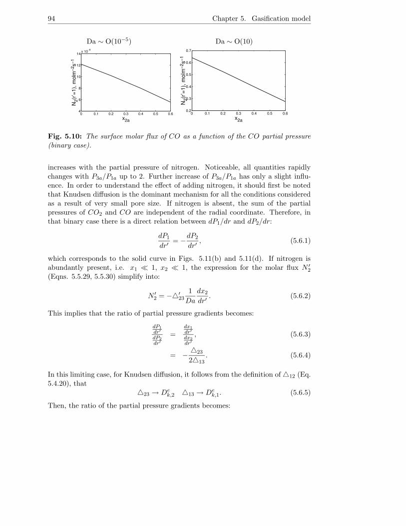
94 Chapter 5. Gasification model
Da ∼ O(10−5) Da ∼ O(10)
0 0.1 0.2 0.3 0.4 0.5 0.64
6
8
10
12
14x 10
−6
x2a
N2(
r’=1)
, mol
m−2
s−1
0 0.1 0.2 0.3 0.4 0.5 0.60.2
0.3
0.4
0.5
0.6
0.7
x2a
N2(
r’=1)
, mol
m−2
s−1
Fig. 5.10: The surface molar flux of CO as a function of the CO partial pressure(binary case).
increases with the partial pressure of nitrogen. Noticeable, all quantities rapidlychanges with P3a/P1a up to 2. Further increase of P3a/P1a has only a slight influ-ence. In order to understand the effect of adding nitrogen, it should first be notedthat Knudsen diffusion is the dominant mechanism for all the conditions consideredas a result of very small pore size. If nitrogen is absent, the sum of the partialpressures of CO2 and CO are independent of the radial coordinate. Therefore, inthat binary case there is a direct relation between dP1/dr and dP2/dr:
dP1
dr′= −dP2
dr′, (5.6.1)
which corresponds to the solid curve in Figs. 5.11(b) and 5.11(d). If nitrogen isabundantly present, i.e. x1 1, x2 1, the expression for the molar flux N ′
2
(Eqns. 5.5.29, 5.5.30) simplify into:
N ′2 = −4′
23
1
Da
dx2
dr′. (5.6.2)
This implies that the ratio of partial pressure gradients becomes:
dP1
dr′
dP2
dr′
=dx1
dr′
dx2
dr′
, (5.6.3)
= − 423
2413. (5.6.4)
In this limiting case, for Knudsen diffusion, it follows from the definition of 412 (Eq.5.4.20), that
423 → Dek,2 413 → De
k,1. (5.6.5)
Then, the ratio of the partial pressure gradients becomes:

5.6. Model predictions 95
Da ∼ O(10−5) Da ∼ O(10)
0 0.2 0.4 0.6 0.8 10.998
0.999
1
1.001
1.002
r’
P1/
P1a
(a) CO2
0 0.2 0.4 0.6 0.8 10.3
0.4
0.5
0.6
0.7
0.8
0.9
1
r’
P1/
P1a
(b) CO2
0 0.2 0.4 0.6 0.8 10
0.2
0.4
0.6
0.8
1
1.2x 10
−5
r’
P2/
P1a
(c) CO
0 0.2 0.4 0.6 0.8 10
0.2
0.4
0.6
0.8
1
r’P
2/P
1a(d) CO
0 0.2 0.4 0.6 0.8 10.998
0.999
1
1.001
1.002
r’
P3/
P3a
(e) Nitrogen
0 0.2 0.4 0.6 0.8 10.9
0.92
0.94
0.96
0.98
1
1.02
r’
P3/
P3a
(f) Nitrogen
0 0.2 0.4 0.6 0.8 10
0.2
0.4
0.6
0.8
1
r’
N2’
(g) Flux
0 0.2 0.4 0.6 0.8 10
0.1
0.2
0.3
0.4
0.5
0.6
0.7
r’
N2’
(h) Flux
—— P3a/P1a = 0 -·-·-·-· P3a/P1a = 2
- - - - P3a/P1a = 4 · · · · · · P3a/P1a = 6
Fig. 5.11: Effect of adding CO in the ambient on the non-dimensional partialpressures and molar flux of CO as a function of the radius of the char particle(ternary case).

96 Chapter 5. Gasification model
dP1
dr′
dP2
dr′
= −1
2
423
413= −1
2
Dek,2
Dek,1
= −1
2
√
M1
M2. (5.6.6)
In the expression we have used that Dek is inversely proportional to the square root
of the molar mass. As a consequence we expect the variation of CO2 to be less andthat of CO to increase as is found in Fig. 5.11.
Effect of adding CO In Fig. 5.12 the effect of adding CO on all quantities isillustrated. The arrow symbol points to the direction of increasing ambient partialpressure of CO. In the reaction controlled regime (left column in Fig. 5.12), the
addition of CO has no effect on the mole fractions of CO2 and CO. The dimen-sionless molar flux of CO follows the linear relation with the radial coordinate. Inthe diffusion controlled regime, the gradients of the mole fractions of CO2 and CObecome weakly dependent on the radial coordinate. This is primarily caused by theinhibition effect of CO on the reaction rate. In Fig. 5.13, the surface molar fluxesof CO for two regimes are presented. In both regimes, the addition of CO reducesthe surface molar fluxes.
5.7 Conclusions
In this chapter, a gasification model is described on the basis of Langmuir kineticsand the ’dusty gas’ model. Both char gasification with CO2 (binary case) and witha mixture of CO2/N2 (ternary case) are considered. The effects of the temperature,total pressure and pore size on the intra-particle mole fractions of gaseous species,molar flux of CO and the surface reaction rate are primarily studied by means ofthe model. The most important finding, for both the binary- and the ternary case,is that the gasification of the present materials is always reaction controlled underthe operating conditions of interest, namely T < 2000K, P < 2 bar and rc = 5µm.This is due to small particle size. When large particles are used, the function ofdiffusion should not be overlooked. For the ternary case, adding nitrogen in thediffusion controlled regime slightly promotes diffusion because Knudsen diffusion isthe dominant mechanism for a very small pore size. In fact, the presence of N2
decouples the diffusion processes of CO2 and of CO.

5.7. Conclusions 97
Da ∼ O(10−5) Da ∼ O(10)
0 0.2 0.4 0.6 0.8 10.998
0.999
1
1.001
1.002
r’
P1/
P1a
(a) CO2
0 0.2 0.4 0.6 0.8 10.3
0.4
0.5
0.6
0.7
0.8
0.9
1
r’
P1/
P1a
(b) CO2
0 0.2 0.4 0.6 0.8 10.998
0.999
1
1.001
1.002
r’
P2/
P2a
(c) CO
0 0.2 0.4 0.6 0.8 11
2
3
4
5
6
7
8
r’
P2/
P2a
(d) CO
0 0.2 0.4 0.6 0.8 10
0.2
0.4
0.6
0.8
1
r’
N2’
(e) Flux
0 0.2 0.4 0.6 0.8 10
0.1
0.2
0.3
0.4
0.5
0.6
0.7
r’
N2’
(f) Flux
Fig. 5.12: The non-dimensional partial pressures and molar flux of CO as a func-tion of the radius of the char particle (ternary case).

98 Chapter 5. Gasification model
Da ∼ O(10−5) Da ∼ O(10)
0 0.1 0.2 0.3 0.40.7
0.8
0.9
1
1.1
1.2
1.3
1.4x 10
−5
x2a
N2,
mol
m−2
s−1
0 0.1 0.2 0.3 0.40.35
0.4
0.45
0.5
0.55
0.6
0.65
0.7
x2a
N2,
mol
m−2
s−1
Fig. 5.13: The surface molar flux of CO as a function of the CO partial pressure(ternary case).

Chapter 6
Gasification of theLignocel-derived chars
6.1 Introduction
On the basis of the model prediction in the preceding chapter, it can be expectedthat pore size, particle size, gasification temperature and pressure are importantfactors that influence the char gasification performance. The properties of the char,for example the pore size, is affected by the pyrolysis conditions of the wood. Tocorrelate the pyrolysis conditions with the char gasification reactivity, therefore,the influence of the pyrolysis conditions, e.g. temperature, pressure and hold time,on the char gasification rate are first investigated. On the basis of this work, thegasification reactivities of three chars (Char I, Char II and Char III ) with CO2 arefurther studied. These chars are prepared at final pyrolysis temperatures of 682K,817K and 916K as described in Chapter 3. The SEM and CO2 physisorptionshows that the chars have very narrow pores of the order of 0.5nm. The microporevolume increases with the final pyrolysis temperature and the surface of the charsbecomes more heterogeneous. This infers an increase of the surface area and thenumber of active sites, which consequently results in different reactivities of threechars. This observation will be validated experimentally in this chapter. Further,according to the gasification model, diffusion will not play a role for the gasificationof these chars under the operating conditions of interest. This prediction will alsobe proven experimentally.
A large amount of measurements on biomass pyrolysis and some on char gasificationkinetics have so far been conducted by using a TGA. With TGA the weight loss ofthe parent material is conveniently measured as a function of time. This method isusually used at relatively low temperatures and at atmospheric pressure. In some
99

100 Chapter 6. Gasification of the Lignocel-derived chars
commercial installations, the pyrolysis and the gasification of feedstock sometimesare operated above atmospheric pressure and at high temperatures. In order to beable to study the two processes in a wide temperature and pressure ranges, the gridreactor was designed. A further objective of this work is to test the feasibility ofthe grid reactor to investigate the gasification of biomass.
6.1.1 Review of literature
The literature contains a vast amount of research data dealing with the reactivity ofcoal char prepared under different conditions including temperature and hold time.Limited information concerning the reactivity of the biomass derived char is availableso far. Previous studies on coal char indicated that the char preparation (pyrolysis)conditions may have a strong influence on its reactivity due to the variation ofchemical composition and pore size distribution [58, 75–79]. Char reactivity clearlydepends on pretreatment temperature, char type, pressure and gaseous reactant. Asa reference to the study of the biomass and its derived char, the information withrespect to coal will be summarized.
Effect of pyrolysis temperature At elevated temperatures, carbonization ofcoal occurs and induces both chemical and physical changes in the char sample. Inthe course of the heat treatment, three major changes take place on the coal surface.First, oxygen and hydrogen atoms are lost. Above approximately 973K, all charshave similar C −H −O contents. Most of the oxygen is lost at lower temperatures;heat treatment above 973K is dominated by loss of hydrogen. Thermal annealing(T ≥ 973 − 1373K) is the third change due to heat treatment. Here microporosityand carbon edges are lost via cluster reorganization. The char structure becomesmore graphitic; hence, unpaired surface electrons disappear. Structural defects alsodisappear. Based on the above, we expect heat treatment to reduce the intrinsic charreactivity due to the loss of active sites. Blake et al.[80] found that the reactivityof highly treated chars is nearly constant because of a more homogeneous carbonstructure. Khan [81] compared the reactivity of the chars between 723K and 1173Kin a TGA. He found that the the low-temperature chars exhibit a higher reactivitythan the parent coals as well as the high-temperature chars. The reactivity of variouschars can be well correlated with the ratio of H/C. Tomkow et al.[82] investigatedthe internal surface area development for brown coal chars pretreated at 773K and1197K and activated with oxygen. The strong effects of pretreatment temperatureare: (1) a higher temperature causes a more rapid destruction of the molecular sieve;(2) a higher temperature favors micropores: and (3) the overall char reactivity ata larger preparation temperature represents a compromise between reduced activesite area and increased total surface area. The overall chemical reactivity of a char

6.1. Introduction 101
particle depends on the type and concentration of active sites and the pore structure,which in turn determines the local concentration of the gaseous reactant.
Effect of the heating rate Radovic et al.[83] measured the reactivities of dem-ineralized North Dakota lignite chars pyrolyzed at a low heating rate (10Kmin−1)and high heating rate (about 104Kmin−1). They found no difference in the charreactivity between the chars prepared at 1275K under low heating rate conditionwith a hold time of 1h and those under rapid heating rate with a hold time of 5min.Kasaoka et al. concluded that the heating rate has almost no effect on char reactiv-ity from their steam gasification rate measurements of chars pyrolyzed at heatingrates in the range of 5-420Kmin−1 and at temperature below 1123K. By con-trast, a significant influence of the heating rate is found in other researches [84–86].Kojima et al. (cited in Luo et al.[84]) reported that reactivities of chars pyrolyzedwith a high heating rate from high volatile Taiheiyo coal at temperatures ranging1173K-1323K were much higher than those under low heating rate conditions. Ka-jitani and Matsuda [86] (cited in Luo et al. [84]) also reported higher reactivities ofchars prepared from Newlands coal under rapid heating condition compared withlow heating conditions at a temperature of 1673K. Luo et al.[84] studied the pyrol-ysis of coal at different heating rates and measured the char reactivity in a fluidizedbed reactor. It was confirmed that the char reactivity increases with the heatingrate.
Effect of the hold time Hindmarsh et al.[79] performed the pyrolysis of coal ina wire-mesh reactor (similar to the grid reactor) and in an entrained flow reactor(drop tube reactor). The hold time was found to be unimportant.
Effect of the pressure The effect of the pressure on the reactivity of hydropy-rolysis char was investigated by Cai et al. They found that a modest increase ofpressure during hydropyrolysis reduces char reactivity; the resolidification of tarprecursors on exposed particle surfaces appears to give a rather unreactive chartoplayer. With increasing hydropyrolysis pressure above about 40 bar, char reactiv-ities increased probably due to gradual erosion of the unreactive surface depositedchar by hydrogasification reactions. The evidence on the influence of the pressureon the tar evaporation has been obtained by Suuberg et al. [87, 88]. It was foundthat the evaporation of tar species is inhibited by the ambient pressure around theparticle. Indirect evidence also suggests that physical entrainment of tar by evolv-ing gaseous products does contribute to the transport process. If the transport ofthe gaseous products is hindered, the gas-solid reactions may result in chars withdifferent reactivities.

102 Chapter 6. Gasification of the Lignocel-derived chars
On the basis of the above literature results, one can expect that the pyrolysis tem-perature, heating rate and pressure are also important factors on determining thegasification reactivity of chars produced from biomass.
6.2 Experimental scheme
Two types of experiments have been carried out in the grid reactor. In the typeA experiments, the wood particles are pyrolyzed first and subsequently gasified. Itis employed to investigate the effects of the pyrolysis temperature, hold time andpressure on the char reactivity. To further investigate the gasification kinetics ofchar, the type B experiments are carried out. In these experiments, Char I, Char IIand Char III are deposited onto the preheated grid for the gasification. This type ofexperiments provides two advantages over type A. First, the char material producedby the experiments of type A is inadequate for the use of characterizations such asthe physisorption. In the type B experiments, sufficient chars can be produced forboth the gasification and the characterizations by means of the oven as describedin Chapter 3. Moreover, chars can be deposited onto the preheated grid to achievea fast heat-up process, which enables an isothermal gasification process. In thefollowing part, the detailed experimental procedures of the two types of experimentsare described.
Type A A small amount of the Lignocel wood powder was spread out on theplatinum grid. After being evacuated to a pressure lower than 2×10⁻⁵ bar, the gridreactor is filled with N2 up to the required pressure. Then the grid is powered andthe pyrolysis starts when the temperature is sufficiently high. After the pyrolysis,the power is turned off and the reactor is evacuated and filled with CO2 up to1 bar. The power is then turned on again and the char left on the grid will start thegasification process when the temperature is high enough. A series of experimentshas been carried out on the basis of the standard pyrolysis and gasification conditionsdefined in Table 6.1. Each individual experiment consists of two separate separateparts: pyrolysis of the wood powder and subsequent char gasification. By changing
Table 6.1: Standard pyrolysis and gasification conditions.
Parameters Pyrolysis Gasification
Temperature, K 980 ± 20 1420 ± 20
Pressure, bar 1 1
Composition of the reactant gas, % 100%, N2 100%, CO2
Hold time, s 60 till complete gasification
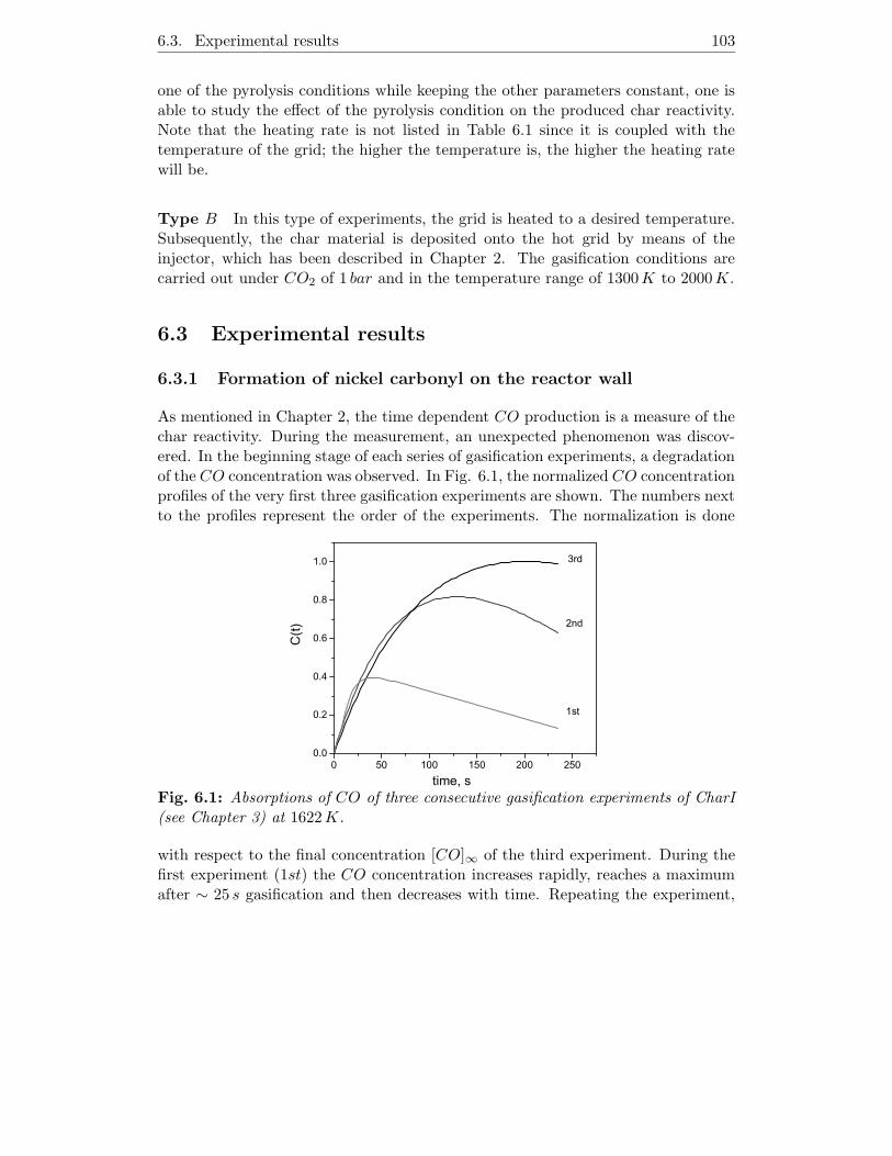
6.3. Experimental results 103
one of the pyrolysis conditions while keeping the other parameters constant, one isable to study the effect of the pyrolysis condition on the produced char reactivity.Note that the heating rate is not listed in Table 6.1 since it is coupled with thetemperature of the grid; the higher the temperature is, the higher the heating ratewill be.
Type B In this type of experiments, the grid is heated to a desired temperature.Subsequently, the char material is deposited onto the hot grid by means of theinjector, which has been described in Chapter 2. The gasification conditions arecarried out under CO2 of 1 bar and in the temperature range of 1300K to 2000K.
6.3 Experimental results
6.3.1 Formation of nickel carbonyl on the reactor wall
As mentioned in Chapter 2, the time dependent CO production is a measure of thechar reactivity. During the measurement, an unexpected phenomenon was discov-ered. In the beginning stage of each series of gasification experiments, a degradationof the CO concentration was observed. In Fig. 6.1, the normalized CO concentrationprofiles of the very first three gasification experiments are shown. The numbers nextto the profiles represent the order of the experiments. The normalization is done
Fig. 6.1: Absorptions of CO of three consecutive gasification experiments of CharI(see Chapter 3) at 1622K.
with respect to the final concentration [CO]∞ of the third experiment. During thefirst experiment (1st) the CO concentration increases rapidly, reaches a maximumafter ∼ 25 s gasification and then decreases with time. Repeating the experiment,

104 Chapter 6. Gasification of the Lignocel-derived chars
the resulting CO concentration profile shows a similar pattern. However, the timeto reach the maximum concentration becomes longer. After the third gasificationexperiment, the degradation of the CO concentration no longer exists. Two differentexplanations are proposed: physical adsorption of CO on the reactor wall and theformation of nickel carbonyl (Ni(CO)4) on the wall. The first one is not very likely.Abundant CO2 is present in the grid reactor. The critical temperature of CO2
(Tc = 304K[38]) is higher than that of CO (Tc = 134K[38]), which suggests thephysisorption of CO2 is easier and will saturate the wall before gasification. There ishardly any unoccupied area left for the adsorption of CO. The second explanationsuggests the formation of Ni(CO)4 as a result of the direct contact between COand the Ni contained in the stainless steel wall. The grid reactor is made of thestainless steel, which contains 12 − 20% of Cr, 7 − 14% of Ni and other elementssuch as Molybdenum and Carbon. It is well known that Ni can easily react withCO to form a carbonyl Ni(CO)4 even at room temperature, according to reference[89]:
Ni+ 4CO Ni(CO)4. (6.3.1)
Ni(CO)4 is a colorless and volatile liquid at room temperature and will decomposeinto Ni and CO as the temperature is above 333K. Suppose that the formationof Ni(CO)4 indeed takes place in the grid reactor, one may expect to observe COproduction by simply heating the grid reactor wall in absence of the char. It isfound that a rise in CO concentration appeared when the grid temperature wasabove 1800K as a consequence of the gradual heat-up of the wall. Now it is seenthat the detrimental effects of the equilibrium reaction 6.3.1 on the determinationof the reaction rate are twofold. The formation of Ni(CO)4 can cause the decreaseof produced CO concentration for a grid temperature below 1800K; At highertemperatures, the decomposition of Ni(CO)4 will produce certain extra amount ofCO. To prevent this problem, different precautions have to be taken in differenttemperature regimes. At low temperatures, it is better to saturate theNi-sites at thereactor wall with CO prior to the gasification experiments. At high temperatures, itis better to heat the grid reactor till the CO adsorbed on the reactor wall is removed.
6.3.2 The effect of pyrolysis conditions on the char reactivity
In Fig. 6.2 the influence of pyrolysis temperature on the burnout time of the chargasification is presented. The pyrolysis temperatures range from 980 to 1250K. Thechar burnout time decreases monotonically with the increase of the pyrolysis tem-perature, which indicates a corresponding increase of the char gasification reactionrate.
In Fig. 6.3 the effect of pyrolysis hold time on char burnout time is shown. Nosignificant influence is found for hold times less than 90 s while a clear increase of

6.3. Experimental results 105
Fig. 6.2: The effect of the pyrolysis temperature on the burnout time of the chargasification.
the char burnout time is found as the hold time exceeds 200 s. When the pyrolysis
Fig. 6.3: The effect of the pyrolysis hold time on the burnout time of the chargasification.
hold time is 600 s, the burnout time is about 120 s indicative of a relatively lowgasification reaction rate. This suggests that the pyrolysis reaction of wood particlesis so fast that there are no dramatic differences on the chemical composition or porestructure among the chars produced for hold times less than 90 s. If the hold timeis prolonged up to 360 s, however, thermoannealing will occur, which in generalhas detrimental effects on the char reactivity because of realignment of the carbonstructure and the loss of active sites.
The effect of pyrolysis pressure on char gasification burnout was assessed by variation

106 Chapter 6. Gasification of the Lignocel-derived chars
of the pressure in the range of 1 bar-17 bar. The result is shown in Fig. 6.4. It isnoteworthy that the char burnout time undergoes a striking increase for pressures up
Fig. 6.4: The effect of the pyrolysis pressure on the burnout time of the char gasi-fication.
to 5 bar, and then goes down when the pressure is above 10 bar. This observationis in agreement with that found with coal hydropyrolysis by Cai et al.[90]. Theeffect of pressure on the char reactivity may be related to the transportation of tarand other gaseous species. In our experiments relatively small wood particles wereused for pyrolysis so that tar and other gaseous products easily escape because ofnegligible mass transport limitation inside the particles. When the pyrolysis pressureincreases, the formed tar will be forced to condense or repolymerize on the exposedfresh surface of the solid particles, which leads to the loss of active sites and effectivearea. As a consequence, the gasification rate decreases with the pressure. When thepressure goes up to even higher values (above 5 bar), however, the mass transfer oftar and other gaseous products within particles will play a much more importantrole during wood pyrolysis. Secondary reactions between solid material and gaseousproducts can take place within the pores, and result in the enlarged porous structureand/or specific surface area for further gasification. Further experimental evidenceis necessary.
6.3.3 Gasification kinetics
The experiments discussed so far gave quantitative information on the relationsbetween the pyrolysis conditions and char gasification reactivity. The pyrolysistemperature is found to have a rather influential role on the produced char reactivity.To understand the observation and for a better comparison between the experimentsand the gasification model predictions, the gasifications of Char I, Char II and Char

6.3. Experimental results 107
III will be studied by performing the type B experiments.
Derivation of kinetic data The gasification of char with CO2 generally takesplace at various temperatures and reactant partial pressures. The intrinsic reactivi-ties of this reaction are supposed to follow a Langmuir equation and can always bereduced to the following form when the pressure is low[91]:
R = kPng , (6.3.2)
where k is the rate constant and Pg is the partial pressure of the reactant gas, i.e.CO2 in our study. In this expression, n is the reaction order with respect to thereactant gas.
In practical kinetics studies of carbon reactions, the concept of overall reactivity isoften used. If one defines the carbon conversion as:
Xc =m0 −m
moαc, (6.3.3)
where m0 is the initial mass of the char particle and m is the mass at any time, andαc is the weight fraction of C in the char, the overall reaction rate is expressed as
R =dXc
dt= − 1
m0αc
dm
dt. (6.3.4)
For reactions on the internal surface, the overall reactivity can also be written as:
R =dXc
dt= ksS(Xc)P
ng , (6.3.5)
where ks is the surface reaction constant, usually related to temperature by theArrhenius equation:
ks = k0 exp(− Ea
RT), (6.3.6)
with the frequency factor k0 and the activation energy Ea. S(Xc) in Eq.6.3.5 isthe transient specific surface area of the particle. It is a function of the carbonconversion and represents the available active sites, accounting for the fraction ofthe occupied surface sites (θ). This can be expressed as, according to Walker etal.[59],
S(Xc) = (1 − θ)SASA, (6.3.7)
where SASA is the active surface area of the char. Replacing S(Xc) in Eq.6.3.5 bythe above expression, the overall reaction rate can be rewritten as
R = k0(1 − θ)SASAPng exp(− Ea
RT). (6.3.8)

108 Chapter 6. Gasification of the Lignocel-derived chars
Therefore, the reaction rate is not only a function of the number of active sites, butalso the active surface area. Let A = k0(1 − θ)SASAP
ng , then the above expression
is reduced to
R = A exp(− Ea
RT). (6.3.9)
In our gasification experiments, the τ90 burnout time was employed as the charac-teristic time for the gasification. Then one can readily write:
1
τ90= A′ exp(− Ea
RT). (6.3.10)
In the above expressions, the parameter S(Xc) is assumed to be constant, whichapparently results in a linear dependence of the conversion on the gasification time.However, the obtained conversion profiles in the present experiments exhibit anexponential shape indicative of the changing S(Xc). The parameter 1
τ90is in this
case a quantitative indicator of the average gasification rate and the parameter A′
in Eq. 6.3.10 is proportional to A in Eq. 6.3.9. By fitting the experimental datato Eq. 6.3.10, the apparent activation energy can be obtained from the slope of theplot of ln( 1
τ90) versus 1
T .
Kinetics data for gasification In Fig. 6.5 the Arrhenius plots for the gasificationof three chars are presented. The obtained apparent activation energies Ea and theparameters A′ are summarized in Table 6.2. It is seen that the pyrolysis temperaturehas a significant influence on the values of Ea and A′ when the pyrolysis temperatureis lower than 800K. The apparent activation energies of chars prepared at highpyrolysis temperatures: Char II (817K) and Char III (916K) are the same, but aremuch higher than that of Char I that was produced at lower pyrolysis temperature
Table 6.2: Apparent activation energies for the gasification of Char I, Char II andChar III.
Sample Ea, kJmol−1 A′, s−1
Char I 92 ± 8 15 ± 10
Char II 208 ± 13 (1.1 ± 1.0) × 105
Char III 208 ± 18 (4.2 ± 6.7) × 105
(682K). This infers that the nature of the active sites becomes less active at elevated
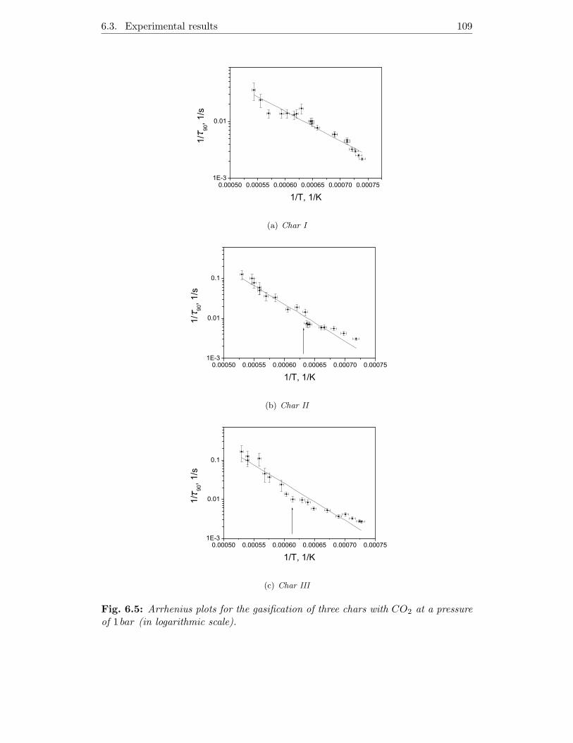
6.3. Experimental results 109
(a) Char I
(b) Char II
(c) Char III
Fig. 6.5: Arrhenius plots for the gasification of three chars with CO2 at a pressureof 1 bar (in logarithmic scale).

110 Chapter 6. Gasification of the Lignocel-derived chars
pyrolysis temperatures. The values of the parameter A′ exhibit a similar trend. Asalready discussed, the parameter A′ depends on the frequency factor, the fractionof the occupied active sites, active surface area, pressure of CO2 and the reactionorder. The pressure of CO2 is constant in the conducted experiments. Therefore,the increase of A′ is possibly caused by the increment of the active surface areaaccompanied by the increase of number of active sites. In agreement with thisobservation, physical adsorption measurements of these three chars infer that atelevated pyrolysis temperatures new micropores are developed, which contributes tothe active surface area. Additionally, it is found that the surface of chars becomesmore heterogeneous when the pyrolysis temperature increases indicating that moreactive sites are produced on the char surface. As the result of the joint contributionof Ea and A′, the gasification rate increases with the pyrolysis temperature up to800K and then levels off.
In the Arrhenius plots of Char II and Char III (Fig. 6.5), a change in slope is seenat a gasification temperature around 1560K. Several factors may account for thisphenomenon: 1) pore diffusion, 2) the change of the gasification mechanism due tothe temperature dependence of both the frequency factor and the activation energyand 3)a catalytic effect. If the gasification is controlled by the pore diffusion, onewill expect a much lower apparent activation energy for the reaction as discussedelsewhere [2]. When the reaction temperature increases, pore diffusion tends to bemore important. As a result, the apparent reaction rate is not affected significantlyby the temperature. This does not agree with the observation in the present case.Therefore, a dominant role of pore diffusion can be excluded. In support of thisexplanation, the gasification model (Chapter 5) also predicts that no diffusion playsa role for the CO2 gasification of the considered chars below 2000K. The secondfactor refers to a transition between the C(O) desorption limited regime and theCO2 adsorption limited regime described by the Langmuir kinetics (see Chapter 5).The Langmuir expression for gasification reads:
Rs =i1i2PCO2
Nt
NA
i1PCO2+ j1PCO + i2
. (6.3.11)
For the gasification experiments performed in this thesis, the partial pressure of COis small compared to that of CO2. The Langmuir expression is then reduced to
Rs =i1i2PCO2
Nt
NA
i1PCO2+ i2
. (6.3.12)
Dividing both the nominator and denominator of Eq. 6.3.13 by i2 yields
Rs =i1PCO2
Nt
NA
i1PCO2
i2+ 1
. (6.3.13)

6.3. Experimental results 111
Wheni1PCO2
i2 1, Rs is reduced to
Rs = Rs,ad = i1PCO2
Nt
NA. (6.3.14)
In this limit the gasification process is determined only by the dissociative chemisorp-
tion of CO2 and exhibits a first-order reaction. In the limiti1PCO2
i2 1,
Rs = Rs,de = i2Nt
NA, (6.3.15)
which corresponds to a desorption of C(O) limited gasification of a zeroth-order.Combining Eqns.6.3.13, 6.3.14 and 6.3.15 yields
1
Rs=
1
Rs,ad+
1
Rs,de. (6.3.16)
The factori1PCO2
i2is in fact the ratio of Rs,ad and Rs,de, which is a function of the
temperature and partial pressure of CO2. In Fig. 6.6 it is plotted as a function ofthe temperature. The partial pressure of CO2 is kept at 1 bar and the kinetics data
1000 1500 2000 25000
0.5
1
1.5
2
2.5
3
T, K
i 1P
CO
2/i 2
Desorption limited
Adsorption limited
Fig. 6.6: The effect of the gasification temperature on the Langmuir mechanism.
are from Barrio et al.[63]. The chemisorption of CO2 is prevailing at higher temper-atures while the desorption of C(O) is dominating at lower temperatures. Previouswork [92] also suggest that the chemisorption of CO2 is potentially faster than thedesorption of C(O) at low temperatures and the latter one is reaction controlling;Due to the higher activation energy of the desorption of C(O), the chemisorption ofCO2 becomes dominating at higher temperatures. In Fig. 6.6, a transition betweenthe two limiting cases takes place at 1553K, which coincides with the temperaturefound in Figs. 6.5(b) and 6.5(c). However, the Arrhenius plot should exhibit alarge slope at low temperatures and a small slope at high temperatures because theactivation energy of the desorption step is relatively higher. Therefore, the non-linear behavior of the Arrhenius plots can not be due to the change of dominating

112 Chapter 6. Gasification of the Lignocel-derived chars
elementary reactions. One can further verify the above explanation by investigatingthe reaction order at two temperature regimes. It is out of the scope of this thesis,but the author would like to indicate the strategy on the identification of the tworegimes. If the gasification is limited by the desorption of CO, the rate will beindependent of the partial pressure of CO2 leading to a zeroth-order reaction; ifthe chemisorption of CO2 is controlling, a non-zeroth order gasification should beobserved. The third factor stresses the importance of the catalytic effect of ashes inthe chars such as alkali metals (K and Na) reported by many researchers[77,93,94].The gasification rate may be represented by the sum of the noncatalytic and thecatalytic reaction rates, according to Radovic et al.[95],
Gasification rate= Non-catalyticgasification rate
+ Catalytic gasifica-tion rate.
The non-catalytic gasification rate is determined by the chemical and physical prop-erties of the char, while the catalytic rate is controlled mainly by alkali metals inthe char. The catalytic effect of the alkali metals depends on the concentration,chemical form, dispersion and so on. Li et al. studied CO2- gasification of a coalchar catalyzed by Na2CO3 and K2CO3. Both catalysts were impregnated on thechar. They found that the catalytic effect diminishes above 1562K for Na2CO3 andabove 1739K for K2CO3. Anita et al.[96] suggested the possibility of loss of thealkali catalyst by evaporation. Therefore, at higher temperatures, the non-catalyticgasification becomes more significant and the material properties are the influentialfactors in determining the gasification rate.
At temperatures below 1560K, the gasification reactions of Char II and Char IIImay be catalyzed by the alkali metals and yield a low activation energy. At highertemperatures, the evaporation of the alkali metals from the solid chars becomesprevailing. Then, the gasification rate is only dependent on the material propertiesof the chars and yields a higher activation energy. For Char I, the situation isdifferent. The gasification rate is controlled mainly by the alkali metals in thetemperature range of interest. The corresponding activation energy is thereforemuch lower.
In the literature, most reported activation energies for the chemically controlledchar-CO2 gasification have values between 170 kJmol−1 and 260 kJmol−1 [63, 73,97–100]. In those researches, particles with dimensions of the order of 1mm areused. The obtained apparent activation energies for Char II and Char III arequite comparable to the reported values and the char particles in the present ex-periments are much smaller. As demonstrated by the gasification model, the CO2-gasification of char particles with the dimension of 10µm is not limited by theintra-particle diffusion under the present conditions. Therefore, it is reasonable to

6.4. Conclusions 113
conclude that the CO2-gasification of Char II and Char III are in a chemically con-trolled regime. The apparent activation energy of Char I is nearly half of the abovementioned values, but agrees well with that determined by Rathmann et al.[99] fromthe CO2 gasification of a straw-derived char. A similar apparent activation energy of100 kJmol−1 is found, which is attributed to the porous structure and the possiblecatalytic effect.
6.4 Conclusions
This chapter merely dealt with the gasification kinetics of the Lignocel-derived charsand the influence of the pyrolysis conditions on the gasification reactivity of the pro-duced chars. Two types of experiments were carried out in a grid reactor. It is foundthat the char reactivity is promoted at elevated pyrolysis temperatures. Hold timeswithin 100 s have no impact on the char gasification reactivity. Longer hold times(> 200 s) become detrimental due to the occurrence of the thermoannealing. Theinfluence of pressure on the char reactivity is most likely related to the transporta-tion of the gaseous products and tar from the particles. Further, the gasificationof three chars produced at different final pyrolysis temperatures is investigated. Inagreement with what has been found previously, the char reactivity tends to behigher at elevated pyrolysis temperature. The reason is that more surface areaand/or number of active sites are produced at higher pyrolysis temperatures as in-dicated by the physical adsorption measurements. In agreement with the previousmodel prediction, diffusion plays no role in the gasification process under presentconditions. A change in the slopes of the Arrhenius plots for Char II and Char IIIis found at the gasification temperature around 1560K, which is presumably dueto the catalytic effect. Further information about the ash composition and the in-fluence of the gasification temperature on the evaporation of ash components willbe very useful. Experiments also manifest that the grid reactor is suitable for thestudy of the intrinsic kinetics of char gasification.


Chapter 7
Concluding remarks and futurework
This chapter draws some conclusions and identifies some areas in which more re-search is necessary.
7.1 Concluding remarks
7.1.1 Fast pyrolysis in the shock tube reactor
• In the study of the fast pyrolysis kinetics of Lignocel wood particles in theshock tube reactor, small wood particles (Dp = 10µm and Hp = 50µm) areused. The particle size is an essential factor in the successful application ofthe shock tube due to the following reasons:
– A small particle size is favorable to a chemically controlled pyrolysis pro-cess, where the homogeneous particle temperature equals the ambient gastemperature and does not vary with time. The estimate of three char-acteristic times is found to be very helpful in identifying different typesof pyrolysis conditions. They are the characteristic pyrolysis time τ3, theheat-up time τ1 and the heat penetration time τ2. If the characteristicpyrolysis time τ3 satisfies τ3 > τ1 > τ2, one speaks of the chemicallycontrolled pyrolysis. In the regime τ1 > τ3 > τ2, a homogeneous particletemperature builds up to the ambient gas temperature with time. In theregime τ2 > τ1, the pyrolysis suffers from the intra-particle heat transferlimitation. Negligible intra-particle heat transfer limitation can be found
115

116 Chapter 7. Concluding remarks and future work
when the particle is smaller than 55µm.
– A small particle size enables the detection at the observation window nearthe end plate. The analysis of the trajectories demonstrates that largerparticles pass through the observation volume and the very small onesare not able to reach the observation window; only those particles withthe diameter around Dp = 10µm are detectable and the number densityof those particles keeps constant. Therefore, the pyrolysis conversion canbe further computed from the extinction measurement.
• Two methods have been developed to derive the kinetics information as totwo types of pyrolysis conditions: τ3 > τ1 > τ2 and τ1 > τ3 > τ2. Theformer process is found at the temperature below 1220K and the latter oneat the temperature above 1220K. In the chemically controlled regime, anapparent activation energy of 106±18.5 kJmol−1 and a pre-exponential factorof (9.8 ± 2.3) × 108 s−1 are obtained. For the other pyrolysis conditions, thedeveloped method still needs to be validated.
• During the pyrolysis in the shock tube reactor, small particles (Dp < 55µm)undergo very fast heating and the pyrolysis is also fast. Under those condi-tions, one is able to observe the early stage of the pyrolysis: primary decom-position of the wood. A comparison between the characteristic tar crackingtime and the reaction time illustrates that secondary tar cracking reactionscan not take place within the test time of about 4ms. The obtained activa-tion energy therefore corresponds to the primary decomposition of the wood.This overcomes the difficulty of the TGA measurement in which the primarydecomposition and the secondary reactions are not distinguished and higheractivation energies are usually found.
• The ratio of the emissivity in two wavelengths is found to be temperatureindependent and most likely composition independent as well. It facilitatesthe temperature measurement of the particle, which will be useful for thevalidation of the second kinetics evaluation method in Appendix E.
7.1.2 Gasification in the grid reactor
In the grid reactor, the effect of the pyrolysis conditions on the produced chargasification reactivity is investigated. Further, the gasification kinetics of threechars produced at different pyrolysis temperatures (682K, 817K and 916K) arestudied. A number of improvements has been made on the sample injection modeand the temperature measurements.

7.1. Concluding remarks 117
• The pyrolysis temperature, pressure and the hold time affect the producedchar gasification reactivity. The gasification rate of the char indeed increaseswith the pyrolysis temperature. Hold times within 100 s have no impact on thechar gasification reactivity, but slower gasification occurs at longer hold timesdue to the occurrence of the thermoannealing. Below 5 bar, the char reactivitydecreases with the pressure. Above this pressure, the char reactivity increaseswith the pressure. This is in agreement with what has been found in coalpyrolysis[90].
• The design and implementation of the char injector enables the char gasifica-tion to occur isothermally. The impact of the heat-up process of the grid itselfon the char gasification rate is therefore avoided.
• The atmospheric gasification of three chars with CO2 is chemically controlledat temperatures below 1900K. The corresponding rates increase with thepyrolysis temperature. Both the apparent activation energy Ea and the expo-nential factor A′ increase with the temperature. The increase of Ea indicatesthat the nature of the active sites becomes less reactive; the increase of A′
suggests the increase of the effective surface area and/or of the number of theactive sites. The above trends are confirmed by the CO2 physical adsorptionof the above three chars. The result indicates that the micropore volume ofchars increases with the final pyrolysis temperatures. The decrease of porehalf-width with the increase of the pyrolysis temperature infers that the in-crement of the micropore volume is mainly caused by the development of newmicropores. In agreement with the production of micropores, the surface ofchars shows a trend toward heterogeneous surface.
• In the temperature range of 1300K-2000K, the gasification of Char II andChar III is in the chemically controlled regime as indicated from the valuesof the apparent activation energies. This is also supported by the predictionof the gasification modelling. A change in the slopes of the Arrhenius plots ofboth chars and the low values activation energy for the gasification of Char Iare presumably due to the catalytic effect.
7.1.3 Gasification modelling
In the gasification model, the dusty gas model and the Langmuir kinetics are in-corporated to describe the diffusion and the chemical reaction mechanisms. It islearned that whether diffusion plays a role in the gasification process depends onmany factors such as the particle size, the pore size, the gasification temperatureand pressure.

118 Chapter 7. Concluding remarks and future work
• The Damkohler number Da can be used as a measure of the significance ofthe diffusion phenomenon. When Da 1, we speak of diffusion controlledgasification; for Da 1, it becomes reaction controlled gasification.
• Under the conditions of interest, namely, T < 2000K, P < 2 bar, the gasifi-cation of the present char of rc = 5µm with CO2 is in the chemical reactioncontrolled regime with or without the presence of nitrogen. This is in agree-ment with the experimental result. The main reason is due to the small particlesize. For large particles, the diffusion will prevail in the gasification process.In the case of char gasification with CO2 at 1400K, it is found that the transi-tion between the reaction controlled regime and the diffusion controlled regimetakes place at a particle radius of 0.65mm. This critical value increases withthe decrease of the gasification temperature.
• In both the binary and the ternary case, the Knudsen diffusion is the domi-nating diffusion mechanism for the narrow pore size of 0.5nm. In the diffusioncontrolled regime, the presence of N2 decouples the diffusion processes of CO2
and of CO. Therefore, the addition of nitrogen promotes the diffusion in acertain range of total pressure (the partial pressure of CO2 is kept constant),but the effect is rather subtle.
7.2 Future work
Both the shock tube reactor and the grid reactor show their potential on studyingthe kinetics of pyrolysis and gasification of biomass. Further work is still necessaryto extend the obtained results.
As to the shock tube experiments:
• With regard to the extinction measurements, there are several effects whichcan degrade the accuracy of this technique. For example, the presence ofash particles become more prevalent after significant burnout and this changecould affect the behavior of the extinction due to the addition of unaccountablescattering sites. This uncertainty should be carefully investigated in order toderive the correct information on the conversion profile for the wood pyrolysis.
• In the analysis of the fast pyrolysis experiments, the heat transfer becomesdominating at a gas temperature above 1220K. Comparison between thepressure and the extinction signal suggests that the so called bifurcation ofthe reflected shock wave also contributes to the heat transfer. To circumventthis problem, Ar is recommended to replace N2 in the test section. Cor-respondingly, the location for the wood injection must be adjusted for themeasurements at the observation window.

7.2. Future work 119
• To measure the particle size observed at the observation window, a microscopeis being built.
Regarding the grid reactor experiments:
• The temperature measurement by means of the thermocouple needs to beimproved. Currently, its measuring junction is clamped to the grid. The loosecontact between the junction and the grid wire may lead to a temperaturedifference. Welding the junction with the thin wire has been found to beextremely difficult and not effective in practice. A tentative experience withthe use of an infrared camera seems to be a very promising way of measuringthe temperature. It is able to make accurate measurements provided theemissivity of the material is known beforehand.
• The model prediction about the effect of N2 addition needs to be validatedexperimentally.
• The change in the slopes of the Arrhenius plots is very likely caused by thecatalytic effect of alkali metals in the chars. Information on the evaporation ofthose catalyst and the interaction between the volatiles and the alkali metalswill be very useful.
• The change of the char reactivity is related to the number of active sites on thechar surface. Quantitative analysis on the dynamic change of the active sitesshall be done by using XPS, TDP , FTIR and solid 13C-NMR or “classical”acid/base titrations.
The gasification model can be improved by
• Introducing the time dependent structure parameters, such as the porosity,inner surface area etc. Two solutions are available. One can measure thestructure parameters as a function of time and implementing results to themodel. However, it certainly requires a lot of experimental effort. The othersolution is to implement the literature reported structure-based models suchas the modified random pore model developed by Gupta and Bhatia[101].
• Including more reactions that certainly play a role in the industrial gasifiers,e.g. the water shift reaction.


Appendix A
Property data bank
This appendix summarises the physical properties used in some of the calculations.
Lignocel wood and the derived char
Wood
kpw = 0.1 [Wm−1K−1] [102]
cpw = 2300 [Jkg−1K−1] [102]
ρpw = 640 [kgm−3] [2]
Char
kpc = 0.68 [Wm−1K−1] [38]
cpc = 1600 [Jkg−1K−1] [102]
ρpc = 450 [kgm−3]
τpc = 1.5
εpc = 0.7
Nitrogen
121

122 Appendix A. Property data bank
M = 28 [kgkmol−1] [70]
Tc = 126.2 [K] [70]
Vc = 89.8 [cm3mol−1] [70]
Pc = 33.9 × 10⁵ [Pa] [70]
Dimp = 0 [debyes] [70]
ω = 0.039 [70]
Pr = 0.71 [26]
Cp(T ) = 1.0059 − 4T + 6 × 10⁻⁷T 2 − 6 ×10⁻¹⁰T 3 + 2 × 10⁻¹³T 4
[kJkg−1K−1] R2 = 1 [70]
k(T ) = 0.0238 + 8 × 10⁻⁵T − 2 × 10⁻⁸T 2 −4 × 10⁻¹¹T 3 + 3 × 10⁻¹⁴T 4
[Wm−1K−1] R2 = 0.9996 [70]
v = 18.5 × 10⁻⁶ [m3mol−1] [70]
Viscosity of N2, µN2
The viscosity of N2, µN2is calculated according to the so-called Chung et al.
method [70]. It can be expressed as
µ = µ∗36.344
√
MN2Tc
V2/3c
, (A.0.1)
where MN2is the molecular weight, Tc the critical temperature, Vc the critical
volume and µ∗ follows
µ∗ =
√T ∗
Ωv
(
Fc
G2+ E6y
)
+ µ∗∗. (A.0.2)
Here,
T ∗ = 1.2593Tr = 1.2593T
Tc, (A.0.3)
Fc = 1 − 0.2756ω + 0.059035µ4r + κ, (A.0.4)
Ωv = 1.16145(T ∗)−0.14874
+0.52487 exp(−0.77320T ∗) + 2.16178 exp(−2.43787T ∗). (A.0.5)
In Eq. (A.0.4), ω is the acentric factor and κ is a special correction for highly polarsubstances such as alcohols and acids. Apparently κ = 0 for N2. The term µr is a

123
dimensionless dipole moment. When Vc is in cm3mole−1, Tc is in Kelvins and thedipole moment Dimp is in debyes,
µr = 131.3Dimp√VcTc
. (A.0.6)
In Eq. (A.0.2),
y =ρVc
6, (A.0.7)
G1 =1 − 0.5y
(1 − y)3, (A.0.8)
G2 =E1[1 − exp(−E4y)]/y + E2G1 exp(E5y) + E3G1
E1E4 + E2 + E3, (A.0.9)
µ∗∗ = E7y2G2 exp
(
E8 +E9
T ∗+
E10
(T ∗)2
)
, (A.0.10)
and the parameters E1 to E10 can be found in [70].
Carbon dioxide
M = 44 [kgkmol−1] [70]
µ(T ) = −2.35619 × 10⁻⁶ + 6.7003 × 10⁻⁸ ×T − 3.2215×−11 ×T 2 + 8.5659× 10⁻¹⁵ × T 3
[kgs−1m−1] R2 = 1 [26]
cp(T ) = 0.48447 + 0.00152. ∗ T − 1.08362 ×10⁻⁶ × T 2 + 3.10411 × 10⁻¹⁰ × T 3
[kJkg−1K−1] R2 = 1 [26]
k(T ) = −0.0073 + 7.55329 × 10⁻⁵ × T +
1.68797× 10⁻⁸ ×T 2 − 1.70192× 10⁻¹¹ ×T 3
[Wm−1K−1] R2 = 0.9999 [26]
v = 26.9 × 10⁻⁶ [m3mol−1] [70]
Carbon monoxide
M = 28 [kgkmol−1] [70]
v = 18.0 × 10⁻⁶ [m3mol−1] [70]

124 Appendix A. Property data bank
Kinetic parameters for gasification
i10 = 1.3 Pa−1s−1 [63]
E1f = 165 kJmol−1 [63]
j10 = 3.6 × 10⁻⁶ Pa−1s−1 [63]
E1b = 20.8 kJmol−1 [63]
i20 = 3.23 × 10⁷ s−1 [63]
E3 = 236 kJmol−1 [63]

Appendix B
Temperature measurement bythermocouple
B.1 Evaluation of heat flow rates
Recalling the heat flow rate balance (Eq. 2.4.28) in the isothermal disk of the grid:
QPt→Tc +QPt +QPt→∞ = QE . (B.1.1)
Each term in this equation was derived in this section, respectively.
Heat flow rate from the grid to the thermocouple at z = 0 : QPt→Tc(0)
The heat flow rate QPt→Tc(0) is
QPt→Tc,0 = −πr2TckTc(dTTc
dz)|z=0. (B.1.2)
The next step is therefore the derivation of the temperature distribution of thethermocouple TTc,z. A cooling fin analysis of the thermocouple with a heat transfercoefficient hTc leads to:
dQTc
dz= −2πrTchTc(TTc − T∞), (B.1.3)
where hTc is the heat transfer coefficient between the thermocouple and the envi-ronment. The Fourier law and the assumption that the thermal conductivity of thethermocouple, kTc, is constant allows us to rewrite equation (B.1.3) as
kTcπr2Tc
d2TTc
dz2− 2πrTchTc(TTc − T∞) = 0. (B.1.4)
125

126 Appendix B. Temperature measurement by thermocouple
The end of the thermocouple (z → ∞) is in thermal equilibrium with the surround-ings:
TTc → T∞. (B.1.5)
The other boundary condition is that the temperature at z = 0 equals that of thegrid and the measured temperature Tm:
TTc = TPt = Tm. (B.1.6)
Restating the entire problem in terms of the excess temperature function
θTc(z) = TTc(z) − T∞ and θm = Tm − T∞, (B.1.7)
leads to
d2θTc
dz2−m2θTc = 0, (B.1.8)
θTc = θm at z = 0, (B.1.9)
θTc → 0 for z → ∞, (B.1.10)
where m =√
2hTc
kTcrTc. The solution of the above differential equation is
θTc(z) = C1 exp(−mz) + C2 exp(mz). (B.1.11)
Since θTc → 0 for z → ∞, we demand C2 = 0. With the other boundary conditionwe find θTc(0) = C1 = θm. Therefore, the final solution becomes
θTc(z) = θm exp(−mz). (B.1.12)
Now QPt→Tc,0 can be calculated as
QPt→Tc = −πr2TckTc(dTTc
dz)|z=0 = −πr2TckTc(
dθ
dz)|z=0,
= πr2TckTc
√
2hTc
kTcrTcθm,
= πr2Tc
√
2hTckTc
rTc(Tm − T∞). (B.1.13)
Heat flow rate from the isothermal disk (r < rTc) to the rest of thegrid (r > rTc): QPt
The heat flow rate QPt reads
QPt = −2πrTcHPtkPtdTPt
dr|r=rTc
. (B.1.14)
B.1. Evaluation of heat flow rates 127
The temperature distribution of the grid was derived subsequently. The steady-stateconservation of energy in the cooling fan approximation for a grid of thickness HPt
with a heat transfer coefficient hPt requires
d
dr(2πrHPtqr) = −4πrhPt(TPt − T∞) + 2πrHPtSe. (B.1.15)
where Se is the electrical power per unit volume. hPt is used considering that onlythe weaved wires contribute to the heat transfer. The derivation of hPt will begiven in detail later. The Fourier law and the assumption that the effective thermalconductivity of the grid, kPt, is constant allow us to rewrite the left-hand side termof equation (B.1.15) as
− d
dr(rdTPt
dr) = − 2hPtr
HPtkPt(TPt − T∞) +
rSe
kPt. (B.1.16)
Developing the left-hand side term of Eq. (B.1.16) and rearranging it gives
r2d2TPt
dr2+ r
dTPt
dr+ r2
[
Se
kPt− 2hPt
HPtkPt(TPt − T∞)
]
= 0. (B.1.17)
The necessary boundary conditions are:
TPt = Tm at r = rTc, (B.1.18)
TPt → TPt,∞ at z → ∞. (B.1.19)
Restating the entire problem in terms of θPt(r) = TPt(r) − T∞ and introducingr′2 = r2 2hPt
HPtkPtyields:
r′2d2θPt
dr′2+ r′
dθPt
dr′− r′2θPt = −r′2HPtSe
2hPt, (B.1.20)
θPt = θPt,rTcat r′Tc =
√
r2Tc
2hPt
HPtkPt, (B.1.21)
θPt → θPt,∞ at z → ∞. (B.1.22)
The general solution to this equation consists of two modified Bessel functions anda particular solution,
θPt(r′) = B1I0(r
′) +B2K0(r′) +
HPtSe
2hPt. (B.1.23)
The Bessel function I0(r′) is exponentially increasing for r′ → ∞, while K0(r
′) isexponentially decreasing to zero. Therefore, we choose B1 = 0. This leads to
θPt(r′) = B2K0(r
′) +HPtSe
2hPt. (B.1.24)

128 Appendix B. Temperature measurement by thermocouple
From the first boundary condition (Eq. (B.1.21)), we know
θPt(∞) = limr′→∞
θPt(r′) =
HPtSe
2hPt. (B.1.25)
Using the remaining boundary condition leads to
θPt(r′Tc) = B2K0(r
′Tc) +
HPtSe
2hPt. (B.1.26)
This yields
B2 =1
K0(r′Tc)
(
θPt(r′Tc) −
HPtSe
2hPt
)
=1
K0(r′Tc)
(
θPt(r′Tc) − θPt(∞)
)
. (B.1.27)
Now we find the following expression for the temperature distribution of the grid:
θPt = θPt,∞ + (θPt,rTc− θPt,∞)
K0(r′)
K0(r′Tc). (B.1.28)
Therefore, the heat flow rate at r = rTc is
QPt = −2πrTcHPtkPtdTPt
dr|r=rTc
= −2πrTcHPtkPtdθPt
dr′|r′=r′
Tc. (B.1.29)
To evaluate this expression we use the recurrence relationK ′0(x) = −K1(x), resulting
in
QPt = 2πrTcHPtkPt(θPt,rTc− θPt,∞)
K1(r′Tc)
K0(r′Tc)
√
2hPt
HPtkPt,
= 2πrTcHPtkPt(Tm − TPt,∞)K1(r
′Tc)
K0(r′Tc)
√
2hPt
HPtkPt. (B.1.30)
Heat dissipation of the grid: Qe
The heat dissipation Qe reads
Qe = πr2TcHPtSe. (B.1.31)
Heat flow rate from the grid to the environment: QPt→∞
The heat flow rate escaping from the grid to the environment QPt→∞ is
QPt→∞ = πr2TchPt(Tm − T∞). (B.1.32)

B.2. Heat transfer coefficients and thermal conductivity 129
Solution
Inserting Eqs. (B.1.13), (B.1.30), (B.1.31) and (B.1.32) into the above balance gives
πr2Tc
√
2hTckTc
rTc(Tm − T∞) +
2πrTcHPtkPt(Tm − TPt,∞)K1(r
′Tc)
K0(r′Tc)
√
2hPt
HPtkPt+
πr2TchPt(Tm − T∞) = πr2TcHPtSe. (B.1.33)
Rearranging equation (B.1.33) yields
Tm − T∞Tm − TPt,∞
=−
√
8hPtHPtkPt
r2Tc
K1(r′Tc)
K0(r′Tc
)+ HPtSe
Tm−TPt,∞
hPt +√
2hTckTc
rTc
. (B.1.34)
Reminding that the temperature of the grid for r → ∞ follows
TPt,∞ = T∞ +HPtSe
2hPt. (B.1.35)
This leads to
Se =2hPt
HPt(TPt,∞ − T∞). (B.1.36)
Substituting it into Eq. B.1.34 yields
Tm − T∞Tm − TPt,∞
=−
√
8hPtHPtkPt
r2Tc
K1(r′Tc)
K0(r′Tc
)− 2hPt
T∞−TPt,∞
Tm−TPt,∞
hPt +√
2hTckTc
rTc
. (B.1.37)
Apart from the physical properties of the grid and the thermocouple, the accuracyof the thermocouple measurement is also dependent on the heat transfer mechanismthrough the values of the heat transfer coefficients hTc and hPt.
B.2 Heat transfer coefficients and thermal conductivity
In the derivation of equation (B.1.37), it is assumed that hTc and hPt are constant.In reality, the overall heat transfer coefficient, which must include convection, con-duction and radiation, is a function of temperature.

130 Appendix B. Temperature measurement by thermocouple
Table B.1: Total emissivity of unoxidized platinum[38].
TPt, K 298 373 773 1273 1773
εPt 0.037 0.047 0.096 0.152 0.191
Radiative heat transfer
The radiant heat transferred from the grid to the environment is given by:
QPt,r = εPtσSeffP t (T 4
Pt − T 4∞), (B.2.1)
in which SeffP t is the effective radiant surface of the wires. It depends on the con-
struction of the grid as shown in Fig. 2.6. The effective radiant surface SeffP t can be
derived as
SeffP t = πDPtLWNPt + πDPtWLNPt − So, (B.2.2)
where So is the overlapped area and NPt the number of wires per meter with a valueof 1/(DPt +Dsp). Now, rewrite Equation (B.2.1) as:
QPt,r = hPt,rLW (TPt − T∞). (B.2.3)
Then hPt,r equals:
hPt,r = εPtσ(2πDPtNPt −So
LW)(T 2
Pt + T 2∞)(TPt + T∞). (B.2.4)
The term So/LW = N2PtD
2Pt is only 4% of the term 2πDPtNPt. It is therefore
reasonable to neglect So/LW . This yields
hPt,r = εPtσ(2πDPtNPt)(T2Pt + T 2
∞)(TPt + T∞). (B.2.5)
The emissivity εPt has the form of
εPt = 0.0001TPt + 0.0093. (B.2.6)
It is obtained by linearly fitting data in Table B.1 and the regression coefficientR2 = 0.9921.
Convective heat transfer
The convective heat transfer from the grid to the ambient is
QPt,c = SeffP t hPtw,c(TPt − T∞), (B.2.7)
B.2. Heat transfer coefficients and thermal conductivity 131
where hPtw,c is the surface averaged heat transfer coefficient of the wire. Replacingequation (B.2.2) into above one gives:
QPt,c = (πDPtNPt + πDPtNPt −So
LW)hPtw,cLW (TPt − T∞). (B.2.8)
Then, the total heat transfer coefficient hPt,c is
hPt,c = (2πDPtNPt −So
LW)hPtw,c. (B.2.9)
Applying the same reasoning, neglecting So/LW yields
hPt,c = 2πDPtNPthPtw,c. (B.2.10)
For the case that the natural convection flow around single cylindrical grid, hPtw,c
reads
hPtw,c =kambNuD,Pt
DPt. (B.2.11)
with the wall averaged Nusselt number NuD,Pt of
NuD,Pt =
0.6 +0.387Ra
1/6D
[1 + (0.559/Pr)9/16]8/27
2
. (B.2.12)
It is valid for 10−5 < RaD < 1012. The Rayleigh number RaD is
RaD =g∆ρD3
Pt
αgν,
=g(ρ∞ − ρg)D
3Pt
αgν. (B.2.13)
Thermal conductivity of the grid, kPt
The total heat transferred to the ambient by the grid reads
QPt = −(LNPt1
4πD2
Pt +WNpt1
4πD2
Pt)kPt,w∂T
∂r. (B.2.14)
where kPt,w is the thermal conductivity of single wire. Therefore, kPt can be derivedas
kPt =LNPt
14πD
2Pt +WNpt
14πD
2Pt
LW. (B.2.15)


Appendix C
Photo-detector responselinearity
In shock tube experiments, photocell or photodiode detectors are employed to mea-sure the light intensity. A linear response, i.e., the generated output voltage U ofthe detector should be directly proportional to the incident light intensity I. It isdesirable but not essential. This is because a linear device is the simplest to cali-brate and the measurements can be interpolated and extrapolated with the greatestaccuracy. The detector response linearity can be verified with the aid of the inversesquare law. It states that the intensity per unit area varies in inverse proportion tothe square of the distance between the light source and the detector, say I = 1/l2.With the aid of this law, a simple setup is constructed as shown in Fig.C.1. A tung-sten lamp is positioned on an optical bench, together with the detector (photocell
Fig. C.1: Experimental setup for measuring the linearity of photo-detector.
light source photo− detector
bench
-l
or photodiode). The distance between the lamp and the detector can be altered by
133

134 Appendix C. Photo-detector response linearity
shifting the lamp along the bench. Suppose the output voltage U is proportional tothe incident intensity I, then, one would find a linear relationship U ∝ 1/l2. Thiswas manifested for the photocell depicted in Fig. C.2. Employing the same method,the response linearity of photodiode to the incident light was also verified.
Fig. C.2: Linearity of photocell.

Appendix D
TGA and DTG curves of biomass
In this appendix TGA and DTG curves of cellulose, lignin and Lignocel wood arepresented. The heating rates are 40Kmin−1 and 60Kmin−1.
135

136 Appendix D. TGA and DTG curves of biomass
(a) Cellulose (b) Lignin
(c) Lignocel wood
Fig. D.1: Pyrolysis of cellulose, lignin and Lignocel wood at three heating rates inthe TGA.
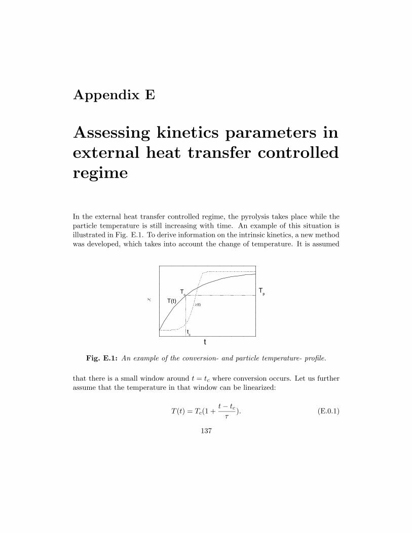
Appendix E
Assessing kinetics parameters inexternal heat transfer controlledregime
In the external heat transfer controlled regime, the pyrolysis takes place while theparticle temperature is still increasing with time. An example of this situation isillustrated in Fig. E.1. To derive information on the intrinsic kinetics, a new methodwas developed, which takes into account the change of temperature. It is assumed
Fig. E.1: An example of the conversion- and particle temperature- profile.
that there is a small window around t = tc where conversion occurs. Let us furtherassume that the temperature in that window can be linearized:
T (t) = Tc(1 +t− tcτ
). (E.0.1)
137
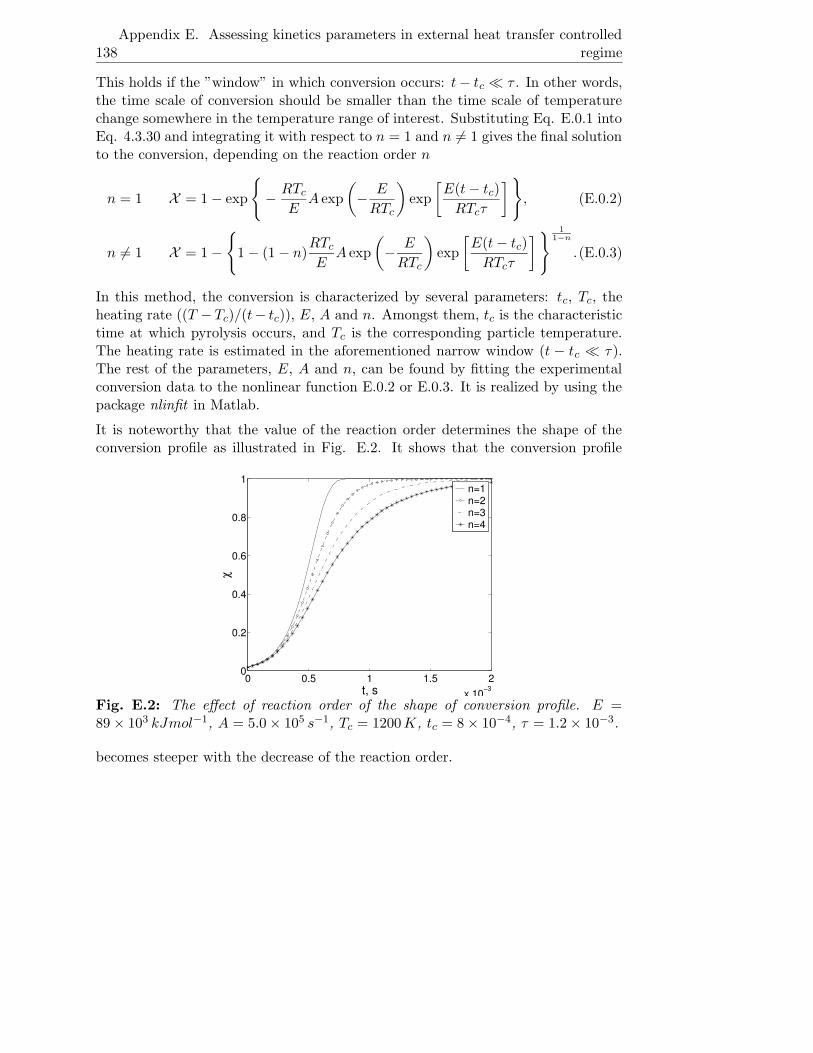
138Appendix E. Assessing kinetics parameters in external heat transfer controlled
regime
This holds if the ”window” in which conversion occurs: t− tc τ . In other words,the time scale of conversion should be smaller than the time scale of temperaturechange somewhere in the temperature range of interest. Substituting Eq. E.0.1 intoEq. 4.3.30 and integrating it with respect to n = 1 and n 6= 1 gives the final solutionto the conversion, depending on the reaction order n
n = 1 X = 1 − exp
− RTc
EA exp
(
− E
RTc
)
exp
[
E(t− tc)
RTcτ
]
, (E.0.2)
n 6= 1 X = 1 −
1 − (1 − n)RTc
EA exp
(
− E
RTc
)
exp
[
E(t− tc)
RTcτ
]
1
1−n
.(E.0.3)
In this method, the conversion is characterized by several parameters: tc, Tc, theheating rate ((T −Tc)/(t− tc)), E, A and n. Amongst them, tc is the characteristictime at which pyrolysis occurs, and Tc is the corresponding particle temperature.The heating rate is estimated in the aforementioned narrow window (t − tc τ).The rest of the parameters, E, A and n, can be found by fitting the experimentalconversion data to the nonlinear function E.0.2 or E.0.3. It is realized by using thepackage nlinfit in Matlab.
It is noteworthy that the value of the reaction order determines the shape of theconversion profile as illustrated in Fig. E.2. It shows that the conversion profile
0 0.5 1 1.5 2x 10⁻³
0
0.2
0.4
0.6
0.8
1
t, s
χ
n=1n=2n=3n=4
Fig. E.2: The effect of reaction order of the shape of conversion profile. E =89 × 103 kJmol−1, A = 5.0 × 10⁵ s−1, Tc = 1200K, tc = 8 × 10⁻⁴, τ = 1.2 × 10⁻³.
becomes steeper with the decrease of the reaction order.

Appendix F
Internal gas flow model
During the pyrolysis of the wood particles, gaseous products (including gas, volatilesand tar) are produced and transported through the pores into the ambient. As tothis process, two phenomena are of interest: the pressure buildup inside the particleand the residence time tresd of the gaseous products. The first phenomenon is relatedto the fragmentation of large particles into small ones, and the second one affectsthe occurrence of the secondary reactions such as the tar cracking reaction. In thisappendix, a quasi-steady state model is given to describe the internal gas flow insidea pore of the wood particle during the pyrolysis process. By means of this model,the influence of the pyrolysis pressure and temperature on the pressure buildup andthe value of tresd are investigated.
F.1 Structure of porous wood particle
In Fig. F.1 the SEM picture of the raw wood particles is shown. Few tracheids witha diameter D ∼ 1µm can be seen in the cross-section of the particles (marked by thewhite circle). In the following model, the considered wood particle is approximatedto have a cylindrical shape with the dimension Dw ∼ 10µm and Hw ∼ 50µm (seeFig. F.2). It contains a number of parallel cylindrical tracheids with a diameterD and a length H = Hw in the longitudinal direction of the wood. The distancebetween the center lines of the adjacent tracheids is Hp = 4D. These tracheidsfunction as the transport tunnels for the gaseous products in the course of thepyrolysis. The internal flow in one of the tunnels is of primary concern.
To simplify the problem, the following assumptions are made. 1) the pyrolysis takesplace isothermally, 2) a quasi-steady state exists, 3) one end of the pore, at x = 0,is assumed to be blind and the other end, at x = H, open. In Fig. F.3 the structure
139
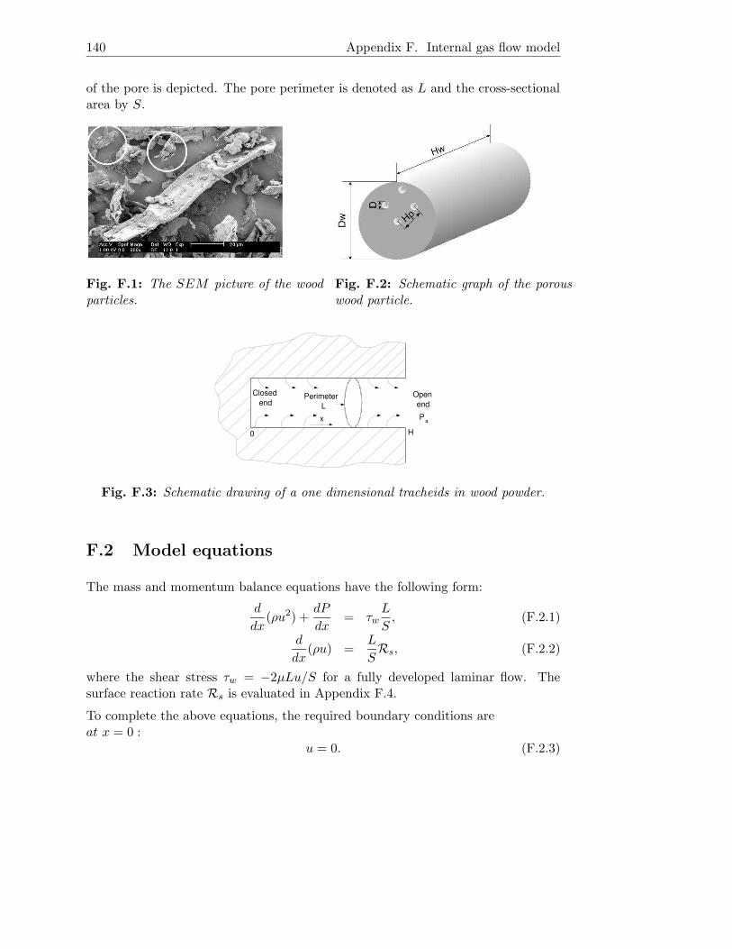
140 Appendix F. Internal gas flow model
of the pore is depicted. The pore perimeter is denoted as L and the cross-sectionalarea by S.
Fig. F.1: The SEM picture of the woodparticles.
Fig. F.2: Schematic graph of the porouswood particle.
Closed end
H 0
x
Open end
P a
Perimeter L
Fig. F.3: Schematic drawing of a one dimensional tracheids in wood powder.
F.2 Model equations
The mass and momentum balance equations have the following form:
d
dx(ρu2) +
dP
dx= τw
L
S, (F.2.1)
d
dx(ρu) =
L
SRs, (F.2.2)
where the shear stress τw = −2µLu/S for a fully developed laminar flow. Thesurface reaction rate Rs is evaluated in Appendix F.4.
To complete the above equations, the required boundary conditions areat x = 0 :
u = 0. (F.2.3)

F.3. Results and conclusions 141
at x = H :
ρ = ρa if u <√RT, else (F.2.4)
u =√RT for ρ > ρa. (F.2.5)
Eq. F.2.4 states that the density (or the pressure) of the gas at the pore exitequals the ambient density (or the ambient pressure) if the gas velocity is below theisothermal speed of sound
√RT (R the specific gas constant). If the gas velocity
at the pore exit becomes sonic, the gas density will exceed the ambient gas densitydue to the “choking effect”. This corresponds to the boundary condition F.2.5.
By introducing the following dimensionless parameters:
x′ =x
H, u′ =
u√RT
, ρ′ =ρ
ρa, R′
s =RsLH
Sρa
√RT
,
eqns. F.2.1-F.2.5 can be rewritten as
d
dx′(
ρ′(u′2 + 1))
= Cu′, (F.2.6)
d
dx′(ρ′u′) = R′
s, (F.2.7)
with the boundary conditions:
u′|x′=0 = 0, (F.2.8)
ρ′|x′=1 = 1 for u′ < 1, (F.2.9)
u′|x′=1 = 1 for ρ′ > 1. (F.2.10)
The parameter C is:
C =2µL2H
S2ρa
√RT
.
The solution of the problem consists of two parts as a result of the two boundaryconditions (Eq. F.2.9 and Eq. F.2.10). They are summarized in Table F.1. Forboth subsonic flow and choked flow, the maximum density ρ′m, which equals themaximum dimensionless pressure P ′
m, is found at the blind side of the pore (x′ = 0).Their solutions are listed in Table F.1 as well.
F.3 Results and conclusions
The data used in the calculation are given in Table F.2. Under the conditions950K ≤ T ≤ 1400K and 1 bar ≤ Pa ≤ 8 bar, the value of R′
s < 1 indicating thatthe choking effect does not occur (see Appendix F.4). Therefore, the solution forthe subsonic flow will be employed.

142 Appendix F. Internal gas flow model
Table F.1: The velocity and density for subsonic flow and choked flow.
Subsonic flow: R′s ≤ 1 Choked flow: R′
s ≥ 1
x′ = u′
R′s
(
R′s+CR′2s +R′3sR′s+u′2C+u′2R′s
)
2R′s+C
2R′s+2Cx′ = u′
(
2R′s+CR′s+u′2C+u′2R′s
)
2R′s+C
2R′s+2C
P ′ = ρ′ =(
R′s+CR′2s +R′3sR′s+R′2s x′2(R′s+C)/ρ′2
)
2R′s+C
2R′s+2CP ′ = ρ′ = R′
s
(
2R′s+CR′s+R′2s x′2(R′s+C)/ρ′2
)
2R′s+C
2R′s+2C
P ′m = ρ′m = (1 + CR′2
s +R′2s )
2R′s+C
2R′s+2C P ′m = ρ′m = R′
s
(
2 + CR′s
)
2R′s+C
2R′s+2C
Table F.2: Physical properties of the wood and kinetic parameters of the pyrolysisused in simulations.
Parameters H D ρw E A
µm µm kgm−3 kJmol−1 s−1
Value 50 10 640 106.5[104] 2.47 × 10⁶[104]
F.3.1 Pressure buildup
In Fig. F.4 the effect of the pyrolysis temperature and the ambient pressure on thedimensionless maximum pressure P ′
m is presented. When the pyrolysis temperatureincreases, the maximum pressure increases due to the higher pyrolysis rate. ForT = 1450K, the maximum pressure is about 17 times larger than the ambientpressure. When the density drop over the pore end is sufficiently high, the poremay be ruptured and a fragmentation of the particles may occur. The increaseof the ambient pressure reduces the maximum pressure. Therefore, the chances ofhaving particle fragmentation is decreasing with the ambient pressure.
F.3.2 Gas residence time
The gas residence time is defined as the ratio of the pore length to the length-averaged velocity: tresd = H/uH , where uH =
∫ H0 udx/
∫ H0 dx. In Fig. F.5 the
effect of the pyrolysis pressure and the temperature on the gas residence time isshown. The gas residence time decreases with the temperature and increases withthe pressure. At Pa = 1 bar, tresd is in the range 67µs-2.5µs in the temperaturerange of 950K-1400K; as Pa increases to 8 bar, tresd increases to 0.43ms-35µs. Theestimate of the gas residence time is very useful for the understanding of the woodpyrolysis mechanism. If the residence time is larger than the characteristic pyrolysistime, the secondary pyrolysis reactions such as tar cracking may occur. Moreover,the tar may also condense in the reacting wood particles when the temperature issufficiently low.

F.4. Appendix: Evaluation of R′s and C 143
1000 1100 1200 1300 1400 15000
5
10
15
20
25
30
T, K
Pm
’
Pa = 1 bar
Pa = 8 bar
Fig. F.4: The effect of the pyrolysis tem-perature and pressure on the density pro-file.
1000 1100 1200 1300 1400 150010
−6
10−5
10−4
10−3
T, K
t resd
, s
Pa = 1 bar
Pa = 8 bar
Fig. F.5: The effect of the pyrolysis tem-perature and the pressure on the residencetime of the gas.
This simple model sheds a good insight on the effect of the pyrolysis temperatureand pressure on the fragmentation of the particle and the residence time of thegaseous products. Its applicability very much depends on the pore structure of thewood particles.
F.4 Appendix: Evaluation of R′s and C
Parameter R′s The parameter R′
s is defined as
R′s =
RsHL
Sρa
√RT
, (F-1)
where the parameter Rs is the surface reaction rate in terms of kgm−2s−1. Infact, the decomposition of biomass is a volumetric reaction process, which can bedescribed by an empirical expression:
Rv = ρwA exp
(
− E
R0T
)
, (F-2)
where A is the frequency factor and E the activation energy, R0 the gas constant.The volumetric reaction rate Rv is related to the surface reaction rate according to
Rs =Rv
Svt=ρw
SvtA exp
(
− E
R0T
)
, (F-3)
where the specific surface area Svt is in terms of the internal area per volume. Thevalue of Svt is estimated as follows:
Svt =number of the tunnels × inner surface area of the tunnels
total volume of the particle=
4ND
D2w
, (F-4)

144 Appendix F. Internal gas flow model
where N is the number of the tunnels present in one particle. Its value is around16 according to Fig. F.2. The ratio L/S can be expressed in terms of the tunneldiameter:
L/S =tunnel perimeter
tunnel cross-section=
4
D. (F-5)
Substituting expressions F-3 and F-5 into the Eqn. F-6 yields
R′s =
(
Dw
D
)2HρwA exp
(
− ER0T
)
NPa
√
R0T
M. (F-6)
Implementing the data in Table F.2, we obtained that the value of R′s is always
smaller than unity under the conditions 950K ≤ T ≤ 1400K and 1 bar ≤ Pa ≤ 8 baras shown in Fig. F.6.
Parameter: C The parameter C is defined in section F.2 as
C =2µL2H
S2ρa
√RT
. (F-7)
With Eq. F-5 and the ideal gas law, the above equation becomes:
C =32µH
D2Pa
√
R0T
M. (F-8)
The estimated value of C is shown in Fig. F.7.
1000 1100 1200 1300 1400 15000
0.2
0.4
0.6
0.8
1
T, K
Rs’
Pa = 1 bar
Pa = 8 bar
Fig. F.6: The value of R′s for the pyrol-
ysis of a wood particle in the temperaturerange 950K-1500K for ambient pressureof 1 bar-8 bar.
1000 1100 1200 1300 1400 150010
1
102
103
T, K
C
Pa = 1 bar
Pa = 8 bar
Fig. F.7: The value of C for the pyrol-ysis of a wood particle in the temperaturerange 950K-1500K for ambient pressureof 1 bar-8 bar.
Bibliography
[1] P. McKendry, “Energy production from biomass (part 1): overview ofbiomass,” Bioresource Technology, vol. 83, pp. 37–46, 2002.
[2] T. B. Reed, A survey of biomass gasification. Volume II - Principles of gasi-fication. Springfield : National Technical Information Service, 1979.
[3] Oregon Department of Energy, “Biomass energy technology.”http://www.energy.state.or.us/biomass/techno.htm.
[4] P. McKendry, “Energy production from biomass (part 3): gasification tech-nologies,” Bioresource Technology, vol. 83, pp. 55–63, 2002.
[5] D. J. Stevens, “Hot gas conditioning: recent progress with larger-scale biomassgasification systems: update and summary of recent progress,” tech. rep.,2001. NREL/SR− 510 − 29952.
[6] R. Warnecke, “Gasification of biomass: comparison of fixed bed and fluidizedbed gasifier,” Biomass and Bioenergy, vol. 18, pp. 489–497, 2000.
[7] J. J. Hos and M. J. Groeneveld, Biomass gasification, pp. 237–255. JohnWiley & Sons Ltd, 1987.
[8] G. Chen, The reactivity of char from rapid heating process under pressure: therole of the time-temperature-environment history of its formation. PhD thesis,Royal Institute of Technology, Sweden, 1998.
[9] A. V. Herzog, T. E. Lipman, and D. M. Kammen, “Rnewable energy sources,”tech. rep. Forerunner Volume “Perspectives and Overview of Life SupportSystems and Sustainable Development,” Part 4C. Energy Resource Scienceand Technology Issues in Sustainable Development Renewable Energy Sources.http://ist-socrates.berkeley.edu/∼rael/eolss.pdf.
[10] K. Maniatis, “Progress in biomass gasification: an overview,” tech. rep., 2001.http://europa.eu.int/comm/energy/res/sectors/doc/bioenergy/km tyrol tony.pdf.
145

146 Bibliography
[11] F.A.C.M.Commissaris, Coal and Char Conversion Rates from Shock Tube Ex-periments. PhD thesis, Eindhoven University of Technology, The Netherlands,1996.
[12] J.H.J.Moors, Pulverised Char Combustion and Gasification at High Temper-atures and Pressures. PhD thesis, Eindhoven University of Technology, TheNetherlands, 1999.
[13] M. J. Antal, H. L. Friedman, and F. E. Rogers, “Kinetics of cellulose pyrolysisin nitrogen and steam,” Comb.Sci. and Tech., vol. 21, pp. 141–152, 1980.
[14] M. Stenseng, A. Jensen, and K. D. Johansen, “Investigation of biomass py-rolysis by thermogravimetric analysis and differential scanning calorimetry,”Journal of Analytical and Applied Pyrolysis, vol. 58-59, pp. 765–780, 2001.
[15] I. Milosavlijevic and E. M. Suuberg, “Cellulose thermal decomposition kinet-ics: Global mass loss kinetics,” Ind.Eng.Chem.Res., no. 34, pp. 1081–1091,1995.
[16] G. Varhegyi, M. J. J. Antal, E. Jakab, and P. Szabo, “Kinetic modellingof biomass pyrolysis,” Journal of Analytical and Applied Pyrolysis, vol. 42,pp. 73–87, 1997.
[17] C. G. J. Hill, An introduction to chemical engineering kinetics and reactordesign. Chichester : Wiley, 1977. Oxford, U.K.
[18] R. Byron, B. Warren, E.Stewart, and E. N.Lightfoot, Transport phenomena.John Wiley & Sons, Inc., 1960. New York.
[19] H. Gunzler and H. U. Gremlich, IR Spectroscopy. Wiley-VCH, 2002. Germany.
[20] A. F. A. Roberts, “A review of kinetic data for the pyrolysis of wood andrelated substances,” Combust. Flame, no. 14, p. 261, 1970.
[21] L. Michalski, K. Eckersdorf, J. Kucharski, and J. McGhee, Temperature mea-surement, vol. second edition. John Wiley & Sons, LTD, 2001. England.
[22] N. R. Keltner and J. V. Beck, “Surface temperature measurement errors,”Heat transfer, vol. 105, no. 7, pp. 1121–1132, 1996.
[23] G. Ben-Dor, O. Igra, and T. Elperin, Handbook of shock waves, Volume I: The-orectical, experimental and numerical techniques. London : Academic Press,2001.
[24] V. E. Banin, Shock tube research on kinetics of pulverised coal particles com-bustion and ignition. PhD thesis, Eindhoven University of Technology, theNetherlands, 1994.

Bibliography 147
[25] T. B. Reed, Low Reynolds number hydrodynamics : with special applicationsto particulate media. Leyden: Noordhoff International, 1973.
[26] A. Bejan, Heat transfer. John Wiley & Sons,Inc., 1993.
[27] M. M. Dubinin and V. A. Astakhov, “Description of adsorption equilibria ofvapors on zeolites over wide ranges of temperature and pressure,” Advancesin Chemistry, vol. 102, pp. 69–85, 1971.
[28] J. Pastor-Villegas and C. J. Duran-Valle, “Pore structure of activated carbonsprepared by carbon dioxide and steam activation at different temperaturesfrom extracted rockrose,” Carbon, vol. 40, no. 3, pp. 397–402, 2002.
[29] D. Cazorla-Amoros, J. Alcaniz-Monge, and A. Linares-Solano, “Characteriza-tion of activated carbon fibers by CO2 adsorption,” Langmuir, vol. 12, no. 2,pp. 2820–2824, 1996.
[30] A. Guillot and F. Stoeckli, “Reference isotherm for high pressure adsorptionof CO2 by carbons at 273 K,” Carbon, vol. 39, pp. 2059–2064, 2001.
[31] P. A. D. Rocca, E. G. Cerrella, P. R. Bonelli, and A. L. Cukierman, “Pyrolysisof hardwoods residues: on kinetics and chars characterization,” Biomass andBioenergy, vol. 16, pp. 79–88, 1999.
[32] S.J.Gregg and K.S.W.Sing, Adsorption, Surface Area and Porosity. AcademicPress, London and New York, 1967.
[33] J. Rouquerol, F. Rodriguez-Reinoso, and K. S. Sing, Characterization ofporous solids. Amsterdam : Elsevier, 1994.
[34] Y. Toda, M. Hatami, S. Toyoda, Y. Yoshida, and M. Honda, “Microporestructure of coal,” Fuel, vol. 50, pp. 187–200, 1971.
[35] C. O. Karacan and E. Okandan, “Adsorption and gas transport in coal mi-crostructure: investigation and evaluation by quantitative x-ray ct imaging,”Fuel, vol. 80, pp. 509–520, 2001.
[36] A. Lopez-Peinado, J. Rivera-Utrilla, J. D. Lopez-Gonzales, and A. M. Ar-jona, “Porous texture characterization of coals and chars,” Adsorption, vol. 2,pp. 31–38, 1985.
[37] J. Hilsenrath, C. W. Beckett, and W. S. Benedict, Tables of thermodynamicand transport properties of air, argon, carbon dioxide, carbon monoxide, hy-drogen, nitrogen, oxygen, and steam. London : Pergamon, 1960.

148 Bibliography
[38] C. W. Robert, Handbook of chemistry and physics, vol. 56th edition. CRCPress, 1975-1976. U.S.A.
[39] M. M. Dubinin, Fundamentals of the theory of physical adsorption of gasesand vapours in micropores. Ricca(Ed.), Acad. Press, 1972. London.
[40] W. Rudzinski and D. Everett, Adsorption of gases on heterogeneous surfaces.London : Academic Press, 1992. London.
[41] G. Varhegyi, M. J. J. Antal, T. Szekely, and P. Szabo, “Kinetics of the thermaldocomposition of cellulose, hemicellulose, and sugar cane bagasse,” Energy andFuels, vol. 3, p. 329, 1989.
[42] T. Kashiwagi and H. Nambu, “Global kinetics constants for thermal oxidativedegradation of a cellulosic paper,” Combustion and Flame, vol. 88, pp. 345–368, 1992.
[43] S. Cooley and M. J. J. Antal, “Kinetics of cellulose pyrolysis in the presenceof nitric oxide,” Journal of Analytical and Applied Pyrolysis, vol. 14, p. 149,1988.
[44] F. J. Kilzer and A. Broido, “Speculations on the nature of cellulose pyrolysis.,”Pyrodynamics, vol. 2, pp. 151–163, 1965.
[45] R. S. Miller and J. Bellan, “A generalized biomass pyrolysis model based onsuperimposed cellulose, hemicellulose and lignin kinetics,” Combust. Sci. andTech., vol. 126, pp. 97–137, 1997.
[46] M.J.Antal, G. Varhegyi, and E. Jakab, “Cellulose pyrolysis kinetics: Revis-ited,” Ind. Eng. Chem. Res, vol. 37, pp. 1267–1275, 1998.
[47] L. H. Sørensen, Fuel reactivity as a function of temperature, pressure andconversion. PhD thesis, Department of Combustion Research, Risø NationalLaboratory, Denmark, 1994.
[48] K. Raveendran, A. Ganesh, and K. C. Khilar, “Pyrolysis characteristics ofbiomass and biomass components,” Fuel, vol. 75, pp. 987–988, 1996.
[49] M. Grønli, M. Stenseng, A. Jensen, and K. Dam-Johansen, “Experimentalinvestigation and kinetic modelling of biomass,” 2nd OUE Lindstrom Sympo-sium, pp. 97–104, 1999.
[50] H. S. Carslaw and J. C. Jaeger, Conduction heat in solids. Clarendon press,2rd ed., 1986. Oxford.

Bibliography 149
[51] F. Shafizadeh and P. P. S. Chin, “Thermal deterioration of wood,” ACS Symp.Ser., pp. 57–81, 1977.
[52] R. Zanzi, K. Sjostrom, and E. Bjornbom, “Rapid high-temperature pyrolysisof biomass in a free-fall reactor,” Fuel, vol. 75, pp. 545–550, 1996.
[53] R. Zanzi, K. Sjostrom, and E. Bjornbom, “Rapid pyrolysis of agriculturalresidues at high temperature,” Biomass and Bioenergy, vol. 23, pp. 357–366,2002.
[54] L.Fagbemi, L.Khezami, and R.Capart, “Pyrolysis products from differentbiomasses: Application to the thermal cracking of tar,” Applied Energy,vol. 69, pp. 293–306, 2001.
[55] S. Ergun, “Kinetics of the reaction of carbon dioxide with carbon,” J. Phys.Chem., vol. 60, pp. 6757–6754, 1956.
[56] M. Mentser and S. Ergun, “Kinetics of oxygen exchange between co2 and coon carbon,” Carbon, vol. 5, pp. 331–337, 1967.
[57] N. M. Laurendeau, “Heterogeneous kinetics of coal char gasification and com-bustion,” vol. 4, pp. 221–270, 1978.
[58] L. R. Radovic, H. Jiang, and A. A. Lizzio, “A transient kinetics study ofchar gasification in carbon dioxide and oxygen,” Energy and Fuels, vol. 5,pp. 68–74, 1991.
[59] P. L. Walker, R. L. J. Taylor, and J. M. Ranish, “An update on the carbon-oxygen reaction,” Carbon, vol. 29, no. 3, pp. 411–421, 1991.
[60] K. J. Huttinger and O. W. Fritz, “The carbon-carbon dioxide reaction: anextended treatment of the active-site concept,” Carbon, vol. 29, pp. 1113–1118, 1991.
[61] A. Montoya, F. Mondragon, and T. N. Truong, “First-principles kinetics of COdesorption from oxygen species on carbonaceous surface,” Physical chemistryA, vol. 106, pp. 4236–4239, 2002.
[62] P. L. Walker, J. F. Rusinko, JR., and L.G.Austin, Gas reactions of carbon,advances in catalysis, vol. 11. Academic Press Inc., 1959. New York.
[63] M. Barrio and J. E. Hustad, “CO2 gasification of birch char andthe effect of CO inhibition on the calculation of chemical kinetics.”http://www.tev.ntnu.no/MariaBarrio/publikasjoner.

150 Bibliography
[64] D. O. Hayward and B. M. W. Trapnell, Chemisorption. London : Butterworth,2rd ed., 1964.
[65] D. Frank-Kamenetskii, Diffusion and heat transfer in chemical kinetics. S.l. :Plenum, 1969. New York.
[66] R. H. Essenhigh, Chemistry of coal utilization: fundamentals of coal combus-tion, vol. Second supplementary volume, ch. 19. Wiley, New York, 1981.
[67] M. Knudsen Ann. Phys., vol. 28, p. 999, 1909.
[68] R. D. Present, Kinetic theory of gases. New York : McGraw-Hill, 1958.
[69] J. C. Maxwell, Scientific papers, vol. 2. New York : Dover, 1952.
[70] R. C. Reid, J. M. Prousnitz, and B. E. Poling, The properties of gases andliquids. McGraw-Hill, 1987. New York.
[71] R. Jackson, Transport in porous catalysts. Amsterdam: Elsevier ScientificPublishing Company, 1977.
[72] J. R. Cash and M. H. Wright, User’s guide for TWPBVP: A code forsolving two-point boundary value problems. In Ode directory of Netlib.http://www.netlib.org/ode/twpbvp.f.
[73] N. Tancredi, T. Cordero, J. Rodrıguez-Mirasol, and J. J. Rodriguez, “co2
gasification of eucalyptus wood chars,” Fuel, vol. 75, no. 13, pp. 1505–1508,1996.
[74] K. Laszlo, K. Josepovits, and E. Tomba, “Analysis of active sites on syntheticcarbon surfaces by various methods,” Analytical Sciences, vol. 17, pp. i1741–i1744, 2001.
[75] K. H. van Heek and H.-J. Muhlen, “Aspects of coal properties and constitutionimportant for gasification,” Fuel, vol. 64, pp. 1405–1414, 1985.
[76] F. Kapteijn and J. Moulijn, Carbon and coal gasification. Dordrecht: MartinusNijhoff Publishers, 1989.
[77] K. Miur, K. Hashimoto, and P. L. Silveston, “Factors affecting the reactivityof coal chars during gasification, and indices representing reactivity,” Fuel,vol. 68, pp. 1461–1475, 1989.
[78] K. M. McDonald, W. D. Hyde, and W. C. Hecker, “Low temperature charoxidation kinetics: effect of preparation method,” Fuel, vol. 71, pp. 319–323,1992.
Bibliography 151
[79] C. J. Hindmarsh, K. M. Thomas, W. X. Wang, H. Y. Cai, A. J. Guell, D. R.Dugwell, and R. A. Kandiyoti, “A comparison of the pyrolysis of coal in wire-mesh and entrained flow reactors,” Fuel, vol. 74, pp. 1185–1190, 1995.
[80] J. H. Blake, G. R. Bopp, J. F. Jones, M. G. Miller, and W. Tambo, “Aspectsof the reactivity of porous carbons with carbon dioxide,” Fuel, vol. 46, p. 115,1967.
[81] M. R. Khan, “Significance of char active surface area for appraising the re-activity of low- and high-temperature chars,” Fuel, vol. 66, pp. 1626–1634,1987.
[82] K. Tomkow, A. Jankowska, F. Czechowski, and T. Siemieniewska, “Activationof brown coal chars with oxygen,” Fuel, vol. 56, pp. 266–270, 1977.
[83] L. R. Radovic, P. L. Walker, and R. G. Jenkins, “Importance of carbon activesites in the gasification of coal chars,” Fuel, vol. 62, pp. 849–856, 1983.
[84] C. Luo, T. Watanabe, M. Nakamura, S. Uemiya, and T. Kojima, “Devel-opment of fbr measurement of char reactiity to carbon dioxide at elevatedtemperatures,” Fuel, vol. 80, pp. 233–243, 2001.
[85] T. Kojima, S. Yamashita, and T. Furusawa Kagaku Kogaku Ronbunshu,vol. 11, p. 735, 1984.
[86] S. Kajitani and H. Matsuda tech. rep., April 1998. Yokosuka Research Labo-ratory Report No. W97020, Japan.
[87] E. M. Suuberg, W. A. Peters, and J. B. Howard, “Product compositions andformation kinetics in rapid pyrolysis of pulverized coal- implications for com-bustion,” pp. 117–130, Combustion Institute, Pittsburgh, 1979.
[88] E. M. Suuberg, P. E. Unger, and W. D. Lilly, “Experimental study on masstransfer from pyrolysing coal particles,” Fuel, vol. 64, pp. 956–962, 1985.
[89] R. Cooperation, “Locating and estimating air emissions from sources ofnickel,” tech. rep., 1984. EPA-450/4-84-007f.
[90] H. Y. Cai, A. J. Guell, I. N. Chatzakis, J. Y. Lim, D. R. Dugwell, andR. Kandiyoti, “Combustion reactivity and morphological change in coal chars:effect of pyrolysis temperature, heating rates and pressure,” Fuel, vol. 75,pp. 15–24, 1996.
[91] G. Q. Lu and D. D. Do, “A kinetic study of coal reject-derived char activationwith CO2, H2O, and air,” Carbon, vol. 30, pp. 21–29, 1992.

152 Bibliography
[92] E. S. Golovina, “The gasification of carbon by carbon dioxide at high temper-atures and pressures,” Carbon, vol. 18, pp. 197–201, 1980.
[93] R. P. W. J. Struis, C. von Scala, S. Stucki, and R. Prins, “Gasification reac-tivity of charcoal with CO2. part I: Conversion and structural phenomena,”Chemical Engineering and Processing, vol. 57, pp. 3581–3592, 2002.
[94] X. Li, H. Wu, J. Hayashi, and C. Li, “Volatilisation and catalytic effects ofalkali and alkaline earth metallic species during the pyrolysis and gasification ofvictorian brown coal. part VI. further investigation into the effects of volatile-char interactions,” Fuel, 2004. Artical in press.
[95] L. R. Radovic, K. Steczko, J. P. L. Walker, and R. G. Jenkins, “A transientkinetics study of char gasification in carbon dioxide and oxygen,” Fuel Pro-cessing Technology, vol. 10, pp. 311–326, 1985.
[96] A. P. Dhupe, A. N. Gokarn, and L. K. Doraiswamy, “Investigations into thecompensation effect at catalystic gasification of active charcoal by carbon diox-ide,” Fuel, vol. 70, pp. 839–844, 2004.
[97] W. F. DeGroot and F. Shafizadeh, “Kinetics of gasification of douglas fir andcottonweed chars by carbon dioxide,” Fuel, vol. 63, pp. 210–216, 1984.
[98] K. Osafune and H. Marsh, “Gasification kinetics of coal chars in carbon diox-ide,” Fuel, vol. 67, pp. 384–388, 1988.
[99] O. Rathmann, P. Hald, J. Bak, J. B. Illerup, E. Gjernes, J. Fjellerup, andA. Olsen, “Combustion and gasification of coal and straw under pressurizedconditions. task 2: determination of kinetic parameters in ptga,” tech. rep.,October 1995. Risø National Laboratory, Risø-R-810(EN),Roskilde, Denmark.
[100] F. Marquez-Montesinos, T. Cordero, J. Rodrıguez, and J. J. Rodrıguez, “CO2
and steam gasification of a grapefruit skin char,” Fuel, vol. 81, pp. 423–429,2002.
[101] J. Srinivasalu and S. K. Bhatia, “A modified discrete random pore modelallowing for different initial surface reactivity,” Carbon, vol. 38, pp. 47–58,2000.
[102] A. M. C. Janse, R. W. J. Westerhout, and W. Prins, “Modelling of flashpyrolysis of a single wood particle,” Chemical Engineering and Processing,vol. 39, pp. 239–252, 2000.
[103] W. E. Schiesser, The numerical method of lines: integration of partial differ-ential equations. Academic Press, Inc, San Diego, California, 1991.

Bibliography 153
[104] F. Thurner and U. Mann, “Kinetic investigation of wood pyrolysis,”Ind.Eng.Chem.Process Des.Dev., vol. 20, pp. 482–488, 1981.


Summary
In this thesis, fast pyrolysis of wood particles and gasification of wood-derived charare investigated. Various experimental and theoretical methods are developed toobtain insight in the kinetics of both processes, and to examine the interaction be-tween the transport phenomena and the chemical reaction. All methods are appliedto Lignocel wood particles and to Lignocel wood-derived char.
Fast pyrolysis of Lignocel wood is studied in a shock tube reactor. Small woodparticles (about 10µm in diameter, 50µm in length) are suspended in nitrogen, priorto the heating of the particles due to shock compression. This compression resultsin a fast heating process that enables to follow the chemical conversion processat constant temperature. Temperatures range from 950K to 1500K at 0.8MPa.A light extinction technique is applied for the time resolved characterization ofthe conversion process and two-wavelength pyrometry is apllied to measure thetemperature of the particles. An analysis is made of the shock induced particlemotion and the heat transfer processes between particles and the surrounding gas. Itis shown that the conversion is chemically controlled at temperatures below 1220K.In this regime, pyrolysis of Lignocel wood particles is well described by a near firstorder reaction with an activation energy of 106±18.5 kJmol−1 and a pre-exponentialfactor of (9.8 ± 2.3) × 108 s−1.
Gasification of wood-derived char is the second main theme of this study. Theexperimental facility used is a closed grid reactor. In such a reactor char particlesare heated on a thin-wired platinum grid up to a maximum temperature of 2000K.In the first series of experiments Lignocel wood particles are first pyrolysed in thegrid reactor and subsequently exposed to a CO2 environment. The gasificationreaction is observed by means of infrared absorption spectroscopy, monitoring theCO-concentration versus time. A restriction of the applied procedure appeared to bethe rather long heating-up time of the grid electrodes and of the grid itself. In orderto circumvent this problem, char is produced in a separate oven and subsequentlydeposited on the preheated grid. To acquire an amount of char, sufficient for itscharacterization as well as for the gasification experiments, a series of chars hasbeen produced at different final pyrolysis temperatures. By means of Scanning
155

156 Summary
Electron Microscopy and the physical adsorption of CO2, the morphology and thepore structure of the chars are characterized. The results show that the producedchar has very narrow pores of the order of 0.5nm. Higher pyrolysis temperaturepromotes the increment of the micropore volume and of the heterogeneous surface.The gasification of these chars with pure CO2 is tested in a temperature range of1300K-1900K at atmospheric pressure in the grid reactor. From the grid reactorexperiments, it is found that the pyrolysis temperature, pressure and hold time haveeffect on the char gasification rate. In the temperature range of 1300K-1900K,no diffusion limitation is found. The activation energies of the chars vary from100 kJmol−1 to 210 kJmol−1, depending on their preparation conditions.
To understand the physics of the gasification process in a complex porous material,a model is developed, which takes into account the interplay between the diffusionof gaseous species and the gasification reaction for the binary case (CO2) and forthe ternary case (CO2/N2), respectively. The diffusion of the gaseous species isdescribed by the dusty gas model and the gasification reaction by the Langmuirkinetics. The effects of the temperature, total pressure and pore size on the intra-particle mole fractions of gaseous species, molar flux of CO and the surface reactionrate are primarily studied by means of the model. For both cases, diffusion plays norole in the gasification of the present chars under the operating conditions of interest,namely T < 2000K, P < 2 bar and rc = 5µm. This is due to the small particle size.Knudsen diffusion is the dominant diffusion process under the conditions mentionedabove. The addition of nitrogen decouples the diffusion processes of CO2 and ofCO. Therefore, diffusion is promoted with the addition of nitrogen but the effect issubtle.

Samenvatting
Dit proefschrift beschrijft onderzoek aan snelle pyrolyse van houtdeeltjes en aanvergassing van houtskooldeeltjes. Verschillende experimentele en theoretische me-thoden zijn ontwikkeld om inzicht te krijgen in de kinetiek van beide processen,en om de wisselwerking tussen de transportprocessen en de chemische reacties teonderzoeken.
Snelle pyrolyse van Lignocel houtdeeltjes is gerealiseerd in een schokbuisreactor.Kleine houtdeeltjes (diameter ongeveer 10µm, lengte 50µm) zijn in suspensie ge-bracht in stiksof, en daarna direkt verhit door schokgolfcompressie. Deze compressieveroorzaakt snelle verhitting van de deeltjes, die het mogelijk maakt om het chemi-sche reactieproces bij constante temperatuur to laten plaatsvinden. De temperatuurwordt gevarieerd tussen 950K en 1500K bij een druk van 0.8MPa. Lichtextinc-tie wordt toegepast om de conversie van de deeltjes te bepalen als funktie van detijd, terwijl de temperatuur van de deeltjes wordt bepaald met twee-golflengten-pyrometrie. Er is een analyse gemaakt van de versnelling en verplaatsing van dedeeltjes als gevolg van de wisselwerking met de door de schokgolven veroorzaaktestroming, en van de daar mee corresponderende overdracht van warmte van gasnaar deeltjes. Aangetoond wordt dat de omzetting volledig door de reactie bepaaldis voor temperaturen beneden 1220K. In dit temperatuurbereik wordt de py-rolyse van houtdeeltjes redelijk goed beschreven door een eerste orde reactie meteen activeringsenergie van 106 ± 18.5 kJmol−1 en een pre-exponentiele factor van(9.8± 2.3)× 108 s−1. De vergassing van de uit het hout verkregen houtskooldeeltjesis het tweede hoofdthema van deze studie. Als experimentele opstelling wordt eengesloten “gridreactor” gebruikt. In een dergelijke reactor worden de houtskool-deeltjes op een uit dunne draden bestaand platina rooster verhit tot een maximumtemperatuur van 2000K. In de eerste serie experimenten zijn Lignocel houtdeel-tjes eerst gepyrolyseerd op het platina rooster en vervolgens blootgesteld aan eenCO2 omgeving. Het vergassingsproces wordt gevolgd door middel van infrarood-absorptiespectroscopie, waarbij de CO2 concentratie wordt geregistreerd. De be-trekkelijk lange opwarmtijd van de electrodes en daarmee van het rooster blijkt eenbeperkende experimentele factor. Om dat probleem te ondervangen is houtskool
157

158 Samenvatting
extern geproduceerd in een speciaal daarvoor gebouwde oven en vervolgens op hetreeds voorverhitte rooster gedeponeerd.
Om een voldoende hoeveelheid houtskool te verkrijgen voor zowel de karakterisatieals voor het vergassingsexperiment, is een series houtskoolmonsters vervaardigdbij verschillende pyrolyse-temperaturen. Door middel van “Scanning Electron Mi-croscopy” en fysische adsorptie van CO2, zijn de morfologie en de poriestructuur vande verschillend houtskoolmonsters gekarakteriseerd. De geproduceerde soorten hout-skool blijken zeer nauwe porien te hebben met diameters van ongeveer 0.5nm. Eenhogere pyrolysetemperatuur blijkt een toename van het porievolume en van het het-erogene oppervlak tot gevolg te hebben. De vergassing van deze typen houtskool isin de “gridreactor” onderzocht in een pure CO2 omgeving in een temperatuurbereikvan 1300K-1900K bij atmosferische druk. Uit de grid reactor experimenten blijkt,dat de pyrolysetemperatuur, pyrolysedruk en “hold time” van invloed zijn op devergassingssnelheid van houtskool. In het temperatuurbereik van 1300K-1900K,blijkt geen diffusiebeperking op te treden. De activeringsenergieen van de verschil-lende houtskoolmonsters blijken te varieren tussen 100 kJmol−1 en 210 kJmol−1,afhankelijk van hun productie condities.
Om het vergassingsproces in een complex materiaal beter te begrijpen is een fy-sisch model ontwikkeld, waarin het samenspel van de diffusie van de bij het procesbetrokken gassen en de vergassingsreactie wordt gemodelleerd, zowel voor het bi-naire geval (CO2/CO) als voor het ternaire geval (CO2/CO/N2). De diffusie in hetporeuze materiaal wordt beschreven met een “dusty gas” model en de vergassingsre-actie met het kinetisch model van Langmuir. De effecten van temperatuur, gasdruken porieafmeting worden door middel van het model onderzocht. Voor de relevantecondities, T < 2000K, P < 2 bar en een poriestraal van 5µm, blijkt diffusie geen rolvan betekenis te spelen. Omdat Knudsen diffusie belangrijker is dan binaire diffusie,blijkt het toevoegen van stikstof de diffusieprocessen van CO2 en van CO volledigte ontkoppelen. Als gevolg daarvan wordt de diffusieweerstand zelfs verminderd,hoewel het effect klein is.

Acknowledgement
In the past four years, many people genuinely showed their interests in this work. Iwould like to take this opportunity to thank all of them.
My utmost appreciation goes to my thesis supervisors: Bram Veefkind, Rini vanDongen and Wijnand Rutgers. I am grateful to Bram, who first introduced me tothe subject of biomass and impressed me with his continuous passion for science.I own a great debt to Rini. As one of my thesis supervisors, he provides me aconstant encouragement, insightful comments, and invaluable suggestions, whichbenefited not only the completion of this thesis, but also my career in a long timeto come. Wijnand, as one of my copromotors, broadens my view with his profoundknowledge and keeps me away from being a research hermit.
During the experimental work involved in this thesis, I’ve learned a great deal frommany people. The shock tube reactor, the grid reactor and the oven are the ma-jor apparatus employed in this work. The experiments would not been completedwithout the technical assistance of Ad Holten and Herman Koolmees, Freek van Uit-tert and Jan Willems. The physical adsorption measurement was assisted by TonSommen. Thermogravimetric analysis was assisted by Duco Bosma and JohannaHeikkinen from the university of Delft. Thanks for sharing your knowledge with meand learning me to work independently as fast as possible.
I am grateful to a number of students, Elaine White, Mirjam Kaizer, Hans vanKuijk and Peter Jonkers, who have brought my attention to various aspects in theencountered problems. I also thank them for their open and active minds. Besidesthe work, exchanging the attitudes towards the cultural difference make my stay inthe Netherlands rejoicing.
I sincerely thank the PhD students that I met in our group. Thanks for igniting theEnglish lunch forum, which broadened my mind and gave me the courage to workwith high spirit. I would like to show my gratitude to Mark Prince, who togetherwith me tried an application for the funding from the Netherlands Organizationfor Scientific Research (NWO). The experience is absolutely bravo! Thank Xiao-quan Wang for providing me the scientific information with his open mind. Thank
159

160 Acknowledgement
Tianming Wen for his wise instruction on SEM measurement.
Thank you Marjan, Brigitte and Anita for a comfortable stay here. The greeting‘NI HAO’ always warms my heart.
I owe a great debt to Mico Hirschberg, Rian van Gaalen and Sjoerd Ypma, whogenerously helped my family during my stay here. Thank you!
Thanks to my dear friends in the Chinese students union in TU/e.
I am deeply indebted to my parents, Shengwu Guo and Caiqin Guo, for their love,open education, encouragement and trust. Thanks for fostering my desire to pursuescientific inquiry and a confident and optimistic life philosophy. I am much deeplyindebted to my dear husband, Haibing, who has encouraged my independence andperseverance with love and understanding. Thanks for his constant company in thislong journey.

Curriculum Vitae
Jieheng Guo was born on October 22, 1975 in Baoji, Shannxi province, China. She
completed her high school education in 1993 at the Petroleum School at Baoji. In
1997 she graduated as a chemical engineer at Northwest University, Xi’an, China.
Her graduation work contributed to the development of an aluminum-based thread
lubricant for the applications at both low and high temperatures. In the same year,
she was recommended to study at the State Key Laboratory of Coal Conversion,
the Institute of Coal Chemistry, Chinese Academy of Sciences, Taiyuan, Shanxi
Province, China. From 1997 to 1998, she went to the Graduate School of the Chinese
Academy of Sciences in Beijing for the study of the basis courses. Afterwards, she
started her research work in the Institute of Coal Chemistry. In 2000 she received
her M.Sc degree under the supervision of Prof. Jianli Yang and Prof. Zhenyu Liu.
The thesis concerned the characterization of an iron-based catalyst for direct coal
liquefaction and was awarded by the Education Bureau of Shanxi province in China
in 2001. During her M.Sc study, she was also involved in the project of evaluating
coal tar-derived bitumen for road building.
Since 2000, she became a research assistant (AIO) in the group of Prof. M.E.H.
van Dongen at the Department of Applied Physics at the Technische Universiteit
Eindhoven.
161