Python Control Documentation - Read the Docs · Welcome to the Python Control Systems Library (python-control) User’s Manual. This manual describes the python- control package,

Python Control DocumentationRelease 0.6d

Python Control Developers

November 30, 2014

Contents

1 Introduction 31.1 Overview of the Toolbox . . . . . . . . . . . . . . . . . . . . . . . . . . . . . . . . . . . . . . . . . 31.2 Some Differences from MATLAB . . . . . . . . . . . . . . . . . . . . . . . . . . . . . . . . . . . . 31.3 Getting Started . . . . . . . . . . . . . . . . . . . . . . . . . . . . . . . . . . . . . . . . . . . . . . 3

2 Python-Control Functions 52.1 Creating System Models . . . . . . . . . . . . . . . . . . . . . . . . . . . . . . . . . . . . . . . . . 52.2 Block Diagram Algebra . . . . . . . . . . . . . . . . . . . . . . . . . . . . . . . . . . . . . . . . . 122.3 Control System Analysis . . . . . . . . . . . . . . . . . . . . . . . . . . . . . . . . . . . . . . . . . 142.4 Frequency Domain Plotting . . . . . . . . . . . . . . . . . . . . . . . . . . . . . . . . . . . . . . . 212.5 Time Domain Simulation . . . . . . . . . . . . . . . . . . . . . . . . . . . . . . . . . . . . . . . . 242.6 Control System Synthesis . . . . . . . . . . . . . . . . . . . . . . . . . . . . . . . . . . . . . . . . 292.7 Model Simplification Tools . . . . . . . . . . . . . . . . . . . . . . . . . . . . . . . . . . . . . . . 302.8 Utility Functions . . . . . . . . . . . . . . . . . . . . . . . . . . . . . . . . . . . . . . . . . . . . . 32

3 Python-Control Classes 333.1 LTI System Class . . . . . . . . . . . . . . . . . . . . . . . . . . . . . . . . . . . . . . . . . . . . . 333.2 State Space Class . . . . . . . . . . . . . . . . . . . . . . . . . . . . . . . . . . . . . . . . . . . . . 343.3 Transfer Function Class . . . . . . . . . . . . . . . . . . . . . . . . . . . . . . . . . . . . . . . . . 353.4 FRD Class . . . . . . . . . . . . . . . . . . . . . . . . . . . . . . . . . . . . . . . . . . . . . . . . 36

4 MATLAB Compatibility Module 394.1 Creating linear models . . . . . . . . . . . . . . . . . . . . . . . . . . . . . . . . . . . . . . . . . . 394.2 Data extraction . . . . . . . . . . . . . . . . . . . . . . . . . . . . . . . . . . . . . . . . . . . . . . 404.3 Conversions . . . . . . . . . . . . . . . . . . . . . . . . . . . . . . . . . . . . . . . . . . . . . . . 404.4 System interconnections . . . . . . . . . . . . . . . . . . . . . . . . . . . . . . . . . . . . . . . . . 404.5 System gain and dynamics . . . . . . . . . . . . . . . . . . . . . . . . . . . . . . . . . . . . . . . . 414.6 Time-domain analysis . . . . . . . . . . . . . . . . . . . . . . . . . . . . . . . . . . . . . . . . . . 414.7 Frequency-domain analysis . . . . . . . . . . . . . . . . . . . . . . . . . . . . . . . . . . . . . . . 414.8 Model simplification . . . . . . . . . . . . . . . . . . . . . . . . . . . . . . . . . . . . . . . . . . . 414.9 Compensator design . . . . . . . . . . . . . . . . . . . . . . . . . . . . . . . . . . . . . . . . . . . 424.10 LQR/LQG design . . . . . . . . . . . . . . . . . . . . . . . . . . . . . . . . . . . . . . . . . . . . 424.11 State-space (SS) models . . . . . . . . . . . . . . . . . . . . . . . . . . . . . . . . . . . . . . . . . 424.12 Frequency response data (FRD) models . . . . . . . . . . . . . . . . . . . . . . . . . . . . . . . . . 424.13 Time delays . . . . . . . . . . . . . . . . . . . . . . . . . . . . . . . . . . . . . . . . . . . . . . . . 434.14 Model dimensions and characteristics . . . . . . . . . . . . . . . . . . . . . . . . . . . . . . . . . . 434.15 Overloaded arithmetic operations . . . . . . . . . . . . . . . . . . . . . . . . . . . . . . . . . . . . 434.16 Matrix equation solvers and linear algebra . . . . . . . . . . . . . . . . . . . . . . . . . . . . . . . . 43

i

4.17 Additional functions . . . . . . . . . . . . . . . . . . . . . . . . . . . . . . . . . . . . . . . . . . . 44

5 Examples 65

6 Indices and tables 67

Python Module Index 69

Python Module Index 71

ii

Python Control Documentation, Release 0.6d

Welcome to the Python Control Systems Library (python-control) User’s Manual. This manual describes the python-control package, including all of the functions defined in the package and examples showing how to use the package.

Contents:

Contents 1


2 Contents

CHAPTER 1

Introduction

Welcome to the Python Control Systems Toolbox (python-control) User’s Manual. This manual contains informa-tion on using the python-control package, including documentation for all functions in the package and examplesillustrating their use.

1.1 Overview of the Toolbox

The python-control package is a set of python classes and functions that implement common operations for the analysisand design of feedback control systems. The initial goal is to implement all of the functionality required to workthrough the examples in the textbook Feedback Systems by Astrom and Murray. A MATLAB compatibility package(control.matlab) is available that provides many of the common functions corresponding to commands available in theMATLAB Control Systems Toolbox.

In addition to the documentation here, there is a project wiki that contains some additional information about how touse the package (including some detailed worked examples):

http://python-control.sourceforge.net

1.2 Some Differences from MATLAB

The python-control package makes use of NumPy and SciPy. A list of general differences between NumPy andMATLAB can be found here:

http://www.scipy.org/NumPy_for_Matlab_Users

In terms of the python-control package more specifically, here are some thing to keep in mind:

• You must include commas in vectors. So [1 2 3] must be [1, 2, 3].

• Functions that return multiple arguments use tuples

• You cannot use braces for collections; use tuples instead

• Transfer functions are currently only implemented for SISO systems; use state space representations for MIMOsystems.

1.3 Getting Started

1. Download latest release from http://sf.net/projects/python-control/files.

3

http://www.cds.caltech.edu/~murray/FBSwiki

http://python-control.sourceforge.net

http://www.scipy.org/NumPy_for_Matlab_Users

http://sf.net/projects/python-control/files


2. Untar the source code in a temporary directory and run ‘python setup.py install’ to build and install the code

3. To see if things are working correctly, run ipython -pylab and run the script ‘examples/secord-matlab.py’. Thisshould generate a step response, Bode plot and Nyquist plot for a simple second order system. (For more detailedtests, run nosetests in the main directory.)

4. To see the commands that are available, run the following commands in ipython:

>>> import control>>> ?control

5. If you want to have a MATLAB-like environment for running the control toolbox, use:

>>> from control.matlab import *>>> ?control.matlab

4 Chapter 1. Introduction

CHAPTER 2

Python-Control Functions

2.1 Creating System Models

Python-control provides a number of methods for creating LTI control systems.ss() create state-space (SS) modelstf() create transfer function (TF) models

2.1.1 System creation

class control.StateSpace(*args)The StateSpace class represents state space instances and functions.

The StateSpace class is used throughout the python-control library to represent systems in state space form. Thisclass is derived from the Lti base class.

The main data members are the A, B, C, and D matrices. The class also keeps track of the number of states (i.e.,the size of A).

Discrete time state space system are implemented by using the ‘dt’ class variable and setting it to the samplingperiod. If ‘dt’ is not None, then it must match whenever two state space systems are combined. Setting dt = 0specifies a continuous system, while leaving dt = None means the system timebase is not specified. If ‘dt’ is setto True, the system will be treated as a discrete time system with unspecified sampling time.

control.ss(*args)Create a state space system.

The function accepts either 1, 4 or 5 parameters:

ss(sys) Convert a linear system into space system form. Always creates a new system, even if sys is alreadya StateSpace object.

ss(A, B, C, D) Create a state space system from the matrices of its state and output equations:

�̇� = 𝐴 · 𝑥+𝐵 · 𝑢𝑦 = 𝐶 · 𝑥+𝐷 · 𝑢

ss(A, B, C, D, dt) Create a discrete-time state space system from the matrices of its state and outputequations:

𝑥[𝑘 + 1] = 𝐴 · 𝑥[𝑘] +𝐵 · 𝑢[𝑘]𝑦[𝑘] = 𝐶 · 𝑥[𝑘] +𝐷 · 𝑢[𝑘𝑖]

5


The matrices can be given as array like data types or strings. Everything that the constructor ofnumpy.matrix accepts is permissible here too.

Parameters sys: Lti (StateSpace or TransferFunction) :

A linear system

A: array_like or string :

System matrix

B: array_like or string :

Control matrix

C: array_like or string :

Output matrix

D: array_like or string :

Feed forward matrix

dt: If present, specifies the sampling period and a discrete time :

system is created

Returns out: StateSpace :

The new linear system

Raises ValueError :

if matrix sizes are not self-consistent

See also:

tf, ss2tf, tf2ss

Examples

>>> # Create a StateSpace object from four "matrices".>>> sys1 = ss("1. -2; 3. -4", "5.; 7", "6. 8", "9.")

>>> # Convert a TransferFunction to a StateSpace object.>>> sys_tf = tf([2.], [1., 3])>>> sys2 = ss(sys_tf)

class control.TransferFunction(*args)The TransferFunction class represents TF instances and functions.

The TransferFunction class is derived from the Lti parent class. It is used throught the python-control library torepresent systems in transfer function form.

The main data members are ‘num’ and ‘den’, which are 2-D lists of arrays containing MIMO numerator anddenominator coefficients. For example,

>>> num[2][5] = numpy.array([1., 4., 8.])

means that the numerator of the transfer function from the 6th input to the 3rd output is set to s^2 + 4s + 8.

Discrete time transfer functions are implemented by using the ‘dt’ class variable and setting it to something otherthan ‘None’. If ‘dt’ has a non-zero value, then it must match whenever two transfer functions are combined. If‘dt’ is set to True, the system will be treated as a discrete time system with unspecified sampling time.

6 Chapter 2. Python-Control Functions

http://docs.scipy.org/doc/numpy/reference/generated/numpy.matrix.html#numpy.matrix


control.tf(*args)Create a transfer function system. Can create MIMO systems.

The function accepts either 1 or 2 parameters:

tf(sys) Convert a linear system into transfer function form. Always creates a new system, even if sys isalready a TransferFunction object.

tf(num, den) Create a transfer function system from its numerator and denominator polynomial coeffi-cients.

If num and den are 1D array_like objects, the function creates a SISO system.

To create a MIMO system, num and den need to be 2D nested lists of array_like objects. (A 3 dimensionaldata structure in total.) (For details see note below.)

tf(num, den, dt) Create a discrete time transfer function system; dt can either be a positive numberindicating the sampling time or ‘True’ if no specific timebase is given.


A linear system

num: array_like, or list of list of array_like :

Polynomial coefficients of the numerator

den: array_like, or list of list of array_like :

Polynomial coefficients of the denominator

Returns out: TransferFunction :


Raises ValueError :

if num and den have invalid or unequal dimensions

TypeError :

if num or den are of incorrect type

See also:

ss, ss2tf, tf2ss

Notes

TodoThe next paragraph contradicts the comment in the example! Also “input” should come before “output” in thesentence:

“from the (j+1)st output to the (i+1)st input”

num[i][j] contains the polynomial coefficients of the numerator for the transfer function from the (j+1)stoutput to the (i+1)st input. den[i][j] works the same way.

The coefficients [2, 3, 4] denote the polynomial 2 · 𝑠2 + 3 · 𝑠+ 4.

2.1. Creating System Models 7


Examples

>>> # Create a MIMO transfer function object>>> # The transfer function from the 2nd input to the 1st output is>>> # (3s + 4) / (6s^2 + 5s + 4).>>> num = [[[1., 2.], [3., 4.]], [[5., 6.], [7., 8.]]]>>> den = [[[9., 8., 7.], [6., 5., 4.]], [[3., 2., 1.], [-1., -2., -3.]]]>>> sys1 = tf(num, den)

>>> # Convert a StateSpace to a TransferFunction object.>>> sys_ss = ss("1. -2; 3. -4", "5.; 7", "6. 8", "9.")>>> sys2 = tf(sys1)

2.1.2 Utility functions and converstions

control.drss(states=1, outputs=1, inputs=1)Create a stable discrete random state space object.

Parameters states: integer :

Number of state variables

inputs: integer :

Number of system inputs

outputs: integer :

Number of system outputs

Returns sys: StateSpace :

The randomly created linear system

Raises ValueError :

if any input is not a positive integer

See also:

rss

Notes

If the number of states, inputs, or outputs is not specified, then the missing numbers are assumed to be 1. Thepoles of the returned system will always have a magnitude less than 1.

control.isctime(sys, strict=False)Check to see if a system is a continuous time system

Parameters sys : LTI system

System to be checked

strict: bool (default = False) :

If strict is True, make sure that timebase is not None

control.isdtime(sys, strict=False)Check to see if a system is a discrete time system







control.issys(object)

control.pade(T, n=1)Create a linear system that approximates a delay.

Return the numerator and denominator coefficients of the Pade approximation.

Parameters T : number

time delay

n : integer

order of approximation

Returns num, den : array

Polynomial coefficients of the delay model, in descending powers of s.

Notes

Based on an algorithm in Golub and van Loan, “Matrix Computation” 3rd. Ed. pp. 572-574.

control.sample_system(sysc, Ts, method=’matched’)Convert a continuous time system to discrete time

Creates a discrete time system from a continuous time system by sampling. Multiple methods of conversion aresupported.

Parameters sysc : linsys

Continuous time system to be converted

Ts : real

Sampling period

method : string

Method to use for conversion: ‘matched’ (default), ‘tustin’, ‘zoh’

Returns sysd : linsys

Discrete time system, with sampling rate Ts

Notes

1.The conversion methods ‘tustin’ and ‘zoh’ require the cont2discrete() function, including in SciPy 0.10.0and above.

2.Additional methods ‘foh’ and ‘impulse’ are planned for future implementation.



Examples

>>> sysc = TransferFunction([1], [1, 2, 1])>>> sysd = sample_system(sysc, 1, method=’matched’)

control.ss2tf(*args)Transform a state space system to a transfer function.


ss2tf(sys) Convert a linear system into space system form. Always creates a new system, even if sys isalready a StateSpace object.

ss2tf(A, B, C, D) Create a state space system from the matrices of its state and output equations.

For details see: ss()

Parameters sys: StateSpace :

A linear system


System matrix


Control matrix


Output matrix


Feedthrough matrix


New linear system in transfer function form

Raises ValueError :

if matrix sizes are not self-consistent, or if an invalid number of arguments is passed in

TypeError :

if sys is not a StateSpace object

See also:

tf, ss, tf2ss

Examples

>>> A = [[1., -2], [3, -4]]>>> B = [[5.], [7]]>>> C = [[6., 8]]>>> D = [[9.]]>>> sys1 = ss2tf(A, B, C, D)

>>> sys_ss = ss(A, B, C, D)>>> sys2 = ss2tf(sys_ss)



control.ssdata(sys)Return state space data objects for a system

Parameters sys: Lti (StateSpace, or TransferFunction) :

LTI system whose data will be returned

Returns (A, B, C, D): list of matrices :

State space data for the system

control.tf2ss(*args)Transform a transfer function to a state space system.


tf2ss(sys) Convert a linear system into transfer function form. Always creates a new system, even if sys isalready a TransferFunction object.

tf2ss(num, den) Create a transfer function system from its numerator and denominator polynomial coef-ficients.

For details see: tf()


A linear system






New linear system in state space form

Raises ValueError :

if num and den have invalid or unequal dimensions, or if an invalid number of argumentsis passed in

TypeError :

if num or den are of incorrect type, or if sys is not a TransferFunction object

See also:

ss, tf, ss2tf

Examples

>>> num = [[[1., 2.], [3., 4.]], [[5., 6.], [7., 8.]]]>>> den = [[[9., 8., 7.], [6., 5., 4.]], [[3., 2., 1.], [-1., -2., -3.]]]>>> sys1 = tf2ss(num, den)

>>> sys_tf = tf(num, den)>>> sys2 = tf2ss(sys_tf)

control.tfdata(sys, **kw)Return transfer function data objects for a system





Returns (num, den): numerator and denominator arrays :

Transfer function coefficients (SISO only)

control.timebase(sys, strict=True)Return the timebase for an Lti system

dt = timebase(sys)

returns the timebase for a system ‘sys’. If the strict option is set to False, dt = True will be returned as 1.

control.timebaseEqual(sys1, sys2)Check to see if two systems have the same timebase

timebaseEqual(sys1, sys2)

returns True if the timebases for the two systems are compatible. By default, systems with timebase ‘None’ arecompatible with either discrete or continuous timebase systems. If two systems have a discrete timebase (dt >0) then their timebases must be equal.

2.2 Block Diagram Algebra

control.feedback(sys1, sys2=1, sign=-1)Feedback interconnection between two I/O systems.

Parameters sys1: scalar, StateSpace, TransferFunction, FRD :

The primary plant.

sys2: scalar, StateSpace, TransferFunction, FRD :

The feedback plant (often a feedback controller).

sign: scalar :

The sign of feedback. sign = -1 indicates negative feedback, and sign = 1 indicatespositive feedback. sign is an optional argument; it assumes a value of -1 if not specified.

Returns out: StateSpace or TransferFunction :

Raises ValueError :

if sys1 does not have as many inputs as sys2 has outputs, or if sys2 does not have asmany inputs as sys1 has outputs

NotImplementedError :

if an attempt is made to perform a feedback on a MIMO TransferFunction object

See also:

series, parallel

Notes

This function is a wrapper for the feedback function in the StateSpace and TransferFunction classes. It callsTransferFunction.feedback if sys1 is a TransferFunction object, and StateSpace.feedback if sys1 is a StateSpace



object. If sys1 is a scalar, then it is converted to sys2‘s type, and the corresponding feedback function is used. Ifsys1 and sys2 are both scalars, then TransferFunction.feedback is used.

control.negate(sys)Return the negative of a system.

Parameters sys: StateSpace, TransferFunction or FRD :

Returns out: StateSpace or TransferFunction :

Notes

This function is a wrapper for the __neg__ function in the StateSpace and TransferFunction classes. The outputtype is the same as the input type.

If both systems have a defined timebase (dt = 0 for continuous time, dt > 0 for discrete time), then the timebasefor both systems must match. If only one of the system has a timebase, the return timebase will be set to matchit.

Examples

>>> sys2 = negate(sys1) # Same as sys2 = -sys1.

control.parallel(sys1, sys2)Return the parallel connection sys1 + sys2.

Parameters sys1: scalar, StateSpace, TransferFunction, or FRD :

sys2: scalar, StateSpace, TransferFunction, or FRD :

Returns out: scalar, StateSpace, or TransferFunction :

Raises ValueError :

if sys1 and sys2 do not have the same numbers of inputs and outputs

See also:

series, feedback

Notes

This function is a wrapper for the __add__ function in the StateSpace and TransferFunction classes. The outputtype is usually the type of sys1. If sys1 is a scalar, then the output type is the type of sys2.


Examples

>>> sys3 = parallel(sys1, sys2) # Same as sys3 = sys1 + sys2.

control.series(sys1, sys2)Return the series connection sys2 * sys1 for –> sys1 –> sys2 –>.

2.2. Block Diagram Algebra 13


Parameters sys1: scalar, StateSpace, TransferFunction, or FRD :

sys2: scalar, StateSpace, TransferFunction, or FRD :

Returns out: scalar, StateSpace, or TransferFunction :

Raises ValueError :

if sys2.inputs does not equal sys1.outputs if sys1.dt is not compatible with sys2.dt

See also:

parallel, feedback

Notes

This function is a wrapper for the __mul__ function in the StateSpace and TransferFunction classes. The outputtype is usually the type of sys2. If sys2 is a scalar, then the output type is the type of sys1.


Examples

>>> sys3 = series(sys1, sys2) # Same as sys3 = sys2 * sys1.

2.3 Control System Analysis

control.acker(A, B, poles)Pole placement using Ackermann method

Call: K = acker(A, B, poles)

Parameters A, B : 2-d arrays

State and input matrix of the system

poles: 1-d list :

Desired eigenvalue locations

Returns K: matrix :

Gains such that A - B K has given eigenvalues

control.ctrb(A, B)Controllabilty matrix

Parameters A, B: array_like or string :

Dynamics and input matrix of the system

Returns C: matrix :

Controllability matrix



Examples

>>> C = ctrb(A, B)

control.care(A, B, Q, R=None, S=None, E=None)(X,L,G) = care(A,B,Q) solves the continuous-time algebraic Riccati equation

A^T X + X A - X B B^T X + Q = 0

where A and Q are square matrices of the same dimension. Further, Q is a symmetric matrix. The functionreturns the solution X, the gain matrix G = B^T X and the closed loop eigenvalues L, i.e., the eigenvalues of A- B G.

(X,L,G) = care(A,B,Q,R,S,E) solves the generalized continuous-time algebraic Riccati equation

A^T X E + E^T X A - (E^T X B + S) R^-1 (B^T X E + S^T) + Q = 0

where A, Q and E are square matrices of the same dimension. Further, Q and R are symmetric matrices. Thefunction returns the solution X, the gain matrix G = R^-1 (B^T X E + S^T) and the closed loop eigenvalues L,i.e., the eigenvalues of A - B G , E.

control.dare(A, B, Q, R, S=None, E=None)(X,L,G) = dare(A,B,Q,R) solves the discrete-time algebraic Riccati equation

A^T X A - X - A^T X B (B^T X B + R)^-1 B^T X A + Q = 0

where A and Q are square matrices of the same dimension. Further, Q is a symmetric matrix. The functionreturns the solution X, the gain matrix G = (B^T X B + R)^-1 B^T X A and the closed loop eigenvalues L, i.e.,the eigenvalues of A - B G.

(X,L,G) = dare(A,B,Q,R,S,E) solves the generalized discrete-time algebraic Riccati equation

A^T X A - E^T X E - (A^T X B + S) (B^T X B + R)^-1 (B^T X A + S^T) +

• Q = 0

where A, Q and E are square matrices of the same dimension. Further, Q and R are symmetric matrices. Thefunction returns the solution X, the gain matrix G = (B^T X B + R)^-1 (B^T X A + S^T) and the closed loopeigenvalues L, i.e., the eigenvalues of A - B G , E.

control.dlyap(A, Q, C=None, E=None)dlyap(A,Q) solves the discrete-time Lyapunov equation

A X A^T - X + Q = 0

where A and Q are square matrices of the same dimension. Further Q must be symmetric.

dlyap(A,Q,C) solves the Sylvester equation

A X Q^T - X + C = 0

where A and Q are square matrices.

dlyap(A,Q,None,E) solves the generalized discrete-time Lyapunov equation

A X A^T - E X E^T + Q = 0

where Q is a symmetric matrix and A, Q and E are square matrices of the same dimension.

control.dcgain(*args)Compute the gain of the system in steady state.

The function takes either 1, 2, 3, or 4 parameters:

Parameters A, B, C, D: array-like :

2.3. Control System Analysis 15


A linear system in state space form.

Z, P, k: array-like, array-like, number :

A linear system in zero, pole, gain form.

num, den: array-like :

A linear system in transfer function form.

sys: Lti (StateSpace or TransferFunction) :

A linear system object.

Returns gain: matrix :

The gain of each output versus each input: 𝑦 = 𝑔𝑎𝑖𝑛 · 𝑢

Notes

This function is only useful for systems with invertible system matrix A.

All systems are first converted to state space form. The function then computes:

𝑔𝑎𝑖𝑛 = −𝐶 ·𝐴−1 ·𝐵 +𝐷

control.evalfr(sys, x)Evaluate the transfer function of an LTI system for a single complex number x.

To evaluate at a frequency, enter x = omega*j, where omega is the frequency in radians

Parameters sys: StateSpace or TransferFunction :

Linear system

x: scalar :

Complex number

Returns fresp: ndarray :

See also:

freqresp, bode

Notes

This function is a wrapper for StateSpace.evalfr and TransferFunction.evalfr.

Examples

>>> sys = ss("1. -2; 3. -4", "5.; 7", "6. 8", "9.")>>> evalfr(sys, 1j)array([[ 44.8-21.4j]])>>> # This is the transfer function matrix evaluated at s = i.

TodoAdd example with MIMO system



control.gram(sys, type)Gramian (controllability or observability)


State-space system to compute Gramian for

type: String :

Type of desired computation. type is either ‘c’ (controllability) or ‘o’ (observability).

Returns gram: array :

Gramian of system

Raises ValueError :

• if system is not instance of StateSpace class

• if type is not ‘c’ or ‘o’

• if system is unstable (sys.A has eigenvalues not in left half plane)

ImportError :

if slycot routin sb03md cannot be found

Examples

>>> Wc = gram(sys,’c’)>>> Wo = gram(sys,’o’)

control.lyap(A, Q, C=None, E=None)X = lyap(A,Q) solves the continuous-time Lyapunov equation

A X + X A^T + Q = 0

where A and Q are square matrices of the same dimension. Further, Q must be symmetric.

X = lyap(A,Q,C) solves the Sylvester equation

A X + X Q + C = 0


X = lyap(A,Q,None,E) solves the generalized continuous-time Lyapunov equation

A X E^T + E X A^T + Q = 0


control.freqresp(sys, omega)Frequency response of an LTI system at multiple angular frequencies.


Linear system

omega: array_like :

List of frequencies

Returns mag: ndarray :

phase: ndarray :

omega: list, tuple, or ndarray :



See also:

evalfr, bode

Notes

This function is a wrapper for StateSpace.freqresp and TransferFunction.freqresp. The output omega is a sortedversion of the input omega.

Examples

>>> sys = ss("1. -2; 3. -4", "5.; 7", "6. 8", "9.")>>> mag, phase, omega = freqresp(sys, [0.1, 1., 10.])>>> magarray([[[ 58.8576682 , 49.64876635, 13.40825927]]])>>> phasearray([[[-0.05408304, -0.44563154, -0.66837155]]])


#>>> sys = rss(3, 2, 2) #>>> mag, phase, omega = freqresp(sys, [0.1, 1., 10.]) #>>> mag[0, 1, :] #array([55.43747231, 42.47766549, 1.97225895]) #>>> phase[1, 0, :] #array([-0.12611087, -1.14294316, 2.5764547]) #>>> # This is the magnitude of the frequency response from the 2nd #>>> # input to the 1st output, and thephase (in radians) of the #>>> # frequency response from the 1st input to the 2nd output, for #>>> # s = 0.1i, i,10i.

control.margin(*args)Calculate gain and phase margins and associated crossover frequencies

Function margin takes either 1 or 3 parameters.

Parameters sys : StateSpace or TransferFunction

Linear SISO system

mag, phase, w : array_like

Input magnitude, phase (in deg.), and frequencies (rad/sec) from bode frequency re-sponse data

Returns gm, pm, Wcg, Wcp : float

Gain margin gm, phase margin pm (in deg), gain crossover frequency (corresponding tophase margin) and phase crossover frequency (corresponding to gain margin), in rad/secof SISO open-loop. If more than one crossover frequency is detected, returns the lowestcorresponding margin.

Examples

>>> sys = ss("1. -2; 3. -4", "5.; 7", "6. 8", "9.")>>> gm, pm, wg, wp = margin(sys)margin: no magnitude crossings found



Todobetter ecample system!

#>>> gm, pm, wg, wp = margin(mag, phase, w)

control.markov(Y, U, M)Calculate the first M Markov parameters [D CB CAB ...] from input U, output Y.

Parameters Y: array_like :

Output data

U: array_like :

Input data

M: integer :

Number of Markov parameters to output

Returns H: matrix :

First M Markov parameters

Notes

Currently only works for SISO

Examples

>>> H = markov(Y, U, M)

control.obsv(A, C)Observability matrix

Parameters A, C: array_like or string :

Dynamics and output matrix of the system

Returns O: matrix :

Observability matrix

Examples

>>> O = obsv(A, C)

control.phase_crossover_frequencies(sys)Compute frequencies and gains at intersections with real axis in Nyquist plot.

Call as: omega, gain = phase_crossover_frequencies()

Returns omega: 1d array of (non-negative) frequencies where Nyquist plot :

intersects the real axis :

gain: 1d array of corresponding gains :



Examples

>>> tf = TransferFunction([1], [1, 2, 3, 4])>>> PhaseCrossoverFrequenies(tf)(array([ 1.73205081, 0. ]), array([-0.5 , 0.25]))

control.pole(sys)Compute system poles.


Linear system

Returns poles: ndarray :

Array that contains the system’s poles.

Raises NotImplementedError :

when called on a TransferFunction object

See also:

zero

Notes

This function is a wrapper for StateSpace.pole and TransferFunction.pole.

control.root_locus(sys, kvect, xlim=None, ylim=None, plotstr=’-‘, Plot=True, PrintGain=True)Calculate the root locus by finding the roots of 1+k*TF(s) where TF is self.num(s)/self.den(s) and each k is anelement of kvect.

Parameters sys : linsys

Linear input/output systems (SISO only, for now)

kvect : gain_range (default = None)

List of gains to use in computing diagram

Plot : boolean (default = True)

If True, plot magnitude and phase

PrintGain: boolean (default = True) :

If True, report mouse clicks when close to the root-locus branches, calculate gain, damp-ing and print

Return values :

————- :

rlist : list of computed root locations

control.stability_margins(sysdata, deg=True, returnall=False, epsw=1e-12)Calculate gain, phase and stability margins and associated crossover frequencies.

Parameters sysdata: linsys or (mag, phase, omega) sequence :

sys [linsys] Linear SISO system

mag, phase, omega [sequence of array_like] Input magnitude, phase, and frequencies(rad/sec) sequence from bode frequency response data



deg=True: boolean :

If true, all input and output phases in degrees, else in radians

returnall=False: boolean :

If true, return all margins found. Note that for frequency data or FRD systems, only onemargin is found and returned.

epsw=1e-12: float :

frequencies below this value are considered static gain, and not returned as margin.

Returns gm, pm, sm, wg, wp, ws: float or array_like :

Gain margin gm, phase margin pm, stability margin sm, and associated crossover fre-quencies wg, wp, and ws of SISO open-loop. If more than one crossover frequency isdetected, returns the lowest corresponding margin. When requesting all margins, thereturn values are array_like, and all margins are returns for linear systems not equal toFRD

control.zero(sys)Compute system zeros.


Linear system

Returns zeros: ndarray :

Array that contains the system’s zeros.


when called on a TransferFunction object or a MIMO StateSpace object

See also:

pole

Notes

This function is a wrapper for StateSpace.zero and TransferFunction.zero.

2.4 Frequency Domain Plotting

2.4.1 Plotting routines

control.bode_plot(syslist, omega=None, dB=None, Hz=None, deg=None, Plot=True, *args,**kwargs)

Bode plot for a system

Plots a Bode plot for the system over a (optional) frequency range.

Parameters syslist : linsys

List of linear input/output systems (single system is OK)

omega : freq_range

Range of frequencies (list or bounds) in rad/sec

2.4. Frequency Domain Plotting 21


dB : boolean

If True, plot result in dB

Hz : boolean

If True, plot frequency in Hz (omega must be provided in rad/sec)

deg : boolean

If True, return phase in degrees (else radians)

Plot : boolean


*args, **kwargs: :

Additional options to matplotlib (color, linestyle, etc)

Returns mag : array (list if len(syslist) > 1)

magnitude

phase : array (list if len(syslist) > 1)

phase

omega : array (list if len(syslist) > 1)

frequency

Notes

1. Alternatively, you may use the lower-level method (mag, phase, freq) = sys.freqresp(freq) to generate thefrequency response for a system, but it returns a MIMO response.

2. If a discrete time model is given, the frequency response is plotted along the upper branch of the unit circle,using the mapping z = exp(j omega dt) where omega ranges from 0 to pi/dt and dt is the discrete time base. Ifnot timebase is specified (dt = True), dt is set to 1.

Examples

>>> sys = ss("1. -2; 3. -4", "5.; 7", "6. 8", "9.")>>> mag, phase, omega = bode(sys)

control.nyquist_plot(syslist, omega=None, Plot=True, color=’b’, labelFreq=0, *args, **kwargs)Nyquist plot for a system

Plots a Nyquist plot for the system over a (optional) frequency range.

Parameters syslist : list of Lti


omega : freq_range


Plot : boolean

If True, plot magnitude

labelFreq : int



Label every nth frequency on the plot

*args, **kwargs: :


Returns real : array

real part of the frequency response array

imag : array

imaginary part of the frequency response array

freq : array

frequencies

Examples

>>> sys = ss("1. -2; 3. -4", "5.; 7", "6. 8", "9.")>>> real, imag, freq = nyquist_plot(sys)

control.gangof4_plot(P, C, omega=None)Plot the “Gang of 4” transfer functions for a system

Generates a 2x2 plot showing the “Gang of 4” sensitivity functions [T, PS; CS, S]

Parameters P, C : Lti

Linear input/output systems (process and control)

omega : array


Returns None :

control.nichols_plot(syslist, omega=None, grid=True)Nichols plot for a system

Plots a Nichols plot for the system over a (optional) frequency range.

Parameters syslist : list of Lti, or Lti


omega : array_like


grid : boolean, optional

True if the plot should include a Nichols-chart grid. Default is True.

Returns None :

2.4.2 Utility functions

control.freqplot.default_frequency_range(syslist)Compute a reasonable default frequency range for frequency domain plots.

Finds a reasonable default frequency range by examining the features (poles and zeros) of the systems in syslist.


2.4. Frequency Domain Plotting 23



Returns omega : array

Range of frequencies in rad/sec

Examples

>>> from matlab import ss>>> sys = ss("1. -2; 3. -4", "5.; 7", "6. 8", "9.")>>> omega = default_frequency_range(sys)

2.5 Time Domain Simulation

Time domain simulation.

This file contains a collection of functions that calculate time responses for linear systems.

2.5.1 Convention for Time Series

This is a convention for function arguments and return values that represent time series: sequences of valuesthat change over time. It is used throughout the library, for example in the functions forced_response(),step_response(), impulse_response(), and initial_response().

Note: This convention is different from the convention used in the library scipy.signal. In Scipy’s conventionthe meaning of rows and columns is interchanged. Thus, all 2D values must be transposed when they are used withfunctions from scipy.signal.

Types:

• Arguments can be arrays, matrices, or nested lists.

• Return values are arrays (not matrices).

The time vector is either 1D, or 2D with shape (1, n):

T = [[t1, t2, t3, ..., tn ]]

Input, state, and output all follow the same convention. Columns are different points in time, rows are differentcomponents. When there is only one row, a 1D object is accepted or returned, which adds convenience for SISOsystems:

U = [[u1(t1), u1(t2), u1(t3), ..., u1(tn)][u2(t1), u2(t2), u2(t3), ..., u2(tn)]......[ui(t1), ui(t2), ui(t3), ..., ui(tn)]]

Same for X, Y

So, U[:,2] is the system’s input at the third point in time; and U[1] or U[1,:] is the sequence of values for the system’ssecond input.

The initial conditions are either 1D, or 2D with shape (j, 1):


http://docs.scipy.org/doc/scipy/reference/signal.html#module-scipy.signal

http://docs.scipy.org/doc/scipy/reference/signal.html#module-scipy.signal


X0 = [[x1][x2]......[xj]]

As all simulation functions return arrays, plotting is convenient:

t, y = step(sys)plot(t, y)

The output of a MIMO system can be plotted like this:

t, y, x = lsim(sys, u, t)plot(t, y[0], label=’y_0’)plot(t, y[1], label=’y_1’)

The convention also works well with the state space form of linear systems. If D is the feedthrough matrix of a linearsystem, and U is its input (matrix or array), then the feedthrough part of the system’s response, can be computed likethis:

ft = D * U

2.5.2 Time responses

control.forced_response(sys, T=None, U=0.0, X0=0.0, transpose=False, **keywords)Simulate the output of a linear system.

As a convenience for parameters U, X0: Numbers (scalars) are converted to constant arrays with the correctshape. The correct shape is inferred from arguments sys and T.

For information on the shape of parameters U, T, X0 and return values T, yout, xout see: Convention for TimeSeries


LTI system to simulate

T: array-like :

Time steps at which the input is defined, numbers must be (strictly monotonic) increas-ing.

U: array-like or number, optional :

Input array giving input at each time T (default = 0).

If U is None or 0, a special algorithm is used. This special algorithm is faster than thegeneral algorithm, which is used otherwise.

X0: array-like or number, optional :

Initial condition (default = 0).

transpose: bool :

If True, transpose all input and output arrays (for backward compatibility with MAT-LAB and scipy.signal.lsim)

**keywords: :

2.5. Time Domain Simulation 25


Additional keyword arguments control the solution algorithm for thedifferential equations. These arguments are passed on to the func-tion scipy.integrate.odeint(). See the documentation forscipy.integrate.odeint() for information about these arguments.

Returns T: array :

Time values of the output.

yout: array :

Response of the system.

xout: array :

Time evolution of the state vector.

See also:

step_response, initial_response, impulse_response

Examples

>>> T, yout, xout = forced_response(sys, T, u, X0)

control.initial_response(sys, T=None, X0=0.0, input=0, output=None, transpose=False, **key-words)

Initial condition response of a linear system

If the system has multiple inputs or outputs (MIMO), one input and one output have to be selected for thesimulation. The parameters input and output do this. All other inputs are set to 0, all other outputs are ignored.

For information on the shape of parameters T, X0 and return values T, yout see: Convention for Time Series

Parameters sys: StateSpace, or TransferFunction :


T: array-like object, optional :

Time vector (argument is autocomputed if not given)

X0: array-like object or number, optional :

Initial condition (default = 0)

Numbers are converted to constant arrays with the correct shape.

input: int :

Index of the input that will be used in this simulation.

output: int :

Index of the output that will be used in this simulation. Set to None to not trim outputs

transpose: bool :


**keywords: :


http://docs.scipy.org/doc/scipy/reference/generated/scipy.integrate.odeint.html#scipy.integrate.odeint



Additional keyword arguments control the solution algorithm for the differential equa-tions. These arguments are passed on to the function lsim(), which in turnpasses them on to scipy.integrate.odeint(). See the documentation forscipy.integrate.odeint() for information about these arguments.

Returns T: array :

Time values of the output

yout: array :

Response of the system

See also:

forced_response, impulse_response, step_response

Examples

>>> T, yout = initial_response(sys, T, X0)

control.step_response(sys, T=None, X0=0.0, input=0, output=None, transpose=False, **keywords)Step response of a linear system

If the system has multiple inputs or outputs (MIMO), one input has to be selected for the simulation. Optionally,one output may be selected. The parameters input and output do this. All other inputs are set to 0, all otheroutputs are ignored.

For information on the shape of parameters T, X0 and return values T, yout see: Convention for Time Series








input: int :


output: int :

Index of the output that will be used in this simulation. Set to None to not trim outputs

transpose: bool :


**keywords: :


Returns T: array :

2.5. Time Domain Simulation 27







yout: array :


See also:

forced_response, initial_response, impulse_response

Examples

>>> T, yout = step_response(sys, T, X0)

2.5.3 Phase portraits

control.phaseplot.phase_plot(odefun, X=None, Y=None, scale=1, X0=None, T=None, lin-grid=None, lintime=None, logtime=None, timepts=None,parms=(), verbose=True)

Phase plot for 2D dynamical systems

Produces a vector field or stream line plot for a planar system.

Call signatures: phase_plot(func, X, Y, ...) - display vector field on meshgrid phase_plot(func, X, Y, scale, ...) -scale arrows phase_plot(func. X0=(...), T=Tmax, ...) - display stream lines phase_plot(func, X, Y, X0=[...],T=Tmax, ...) - plot both phase_plot(func, X0=[...], T=Tmax, lingrid=N, ...) - plot both phase_plot(func,X0=[...], lintime=N, ...) - stream lines with arrows

Parameters func : callable(x, t, ...)

Computes the time derivative of y (compatible with odeint). The function should be thesame for as used for scipy.integrate. Namely, it should be a function of the form dxdt =F(x, t) that accepts a state x of dimension 2 and returns a derivative dx/dt of dimension2.

X, Y: ndarray, optional :

Two 1-D arrays representing x and y coordinates of a grid. These arguments are passedto meshgrid and generate the lists of points at which the vector field is plotted. If absent(or None), the vector field is not plotted.

scale: float, optional :

Scale size of arrows; default = 1

X0: ndarray of initial conditions, optional :

List of initial conditions from which streamlines are plotted. Each initial conditionshould be a pair of numbers.

T: array-like or number, optional :

Length of time to run simulations that generate streamlines. If a single number, thesame simulation time is used for all initial conditions. Otherwise, should be a list oflength len(X0) that gives the simulation time for each initial condition. Default value =50.

lingrid = N or (N, M): integer or 2-tuple of integers, optional :



If X0 is given and X, Y are missing, a grid of arrows is produced using the limits of theinitial conditions, with N grid points in each dimension or N grid points in x and M gridpoints in y.

lintime = N: integer, optional :

Draw N arrows using equally space time points

logtime = (N, lambda): (integer, float), optional :

Draw N arrows using exponential time constant lambda

timepts = [t1, t2, ...]: array-like, optional :

Draw arrows at the given list times

parms: tuple, optional :

List of parameters to pass to vector field: func(x, t, *parms)

See also:

box_grid, Y

control.phaseplot.box_grid(xlimp, ylimp)box_grid generate list of points on edge of box

list = box_grid([xmin xmax xnum], [ymin ymax ynum]) generates a list of points that correspond to a uniformgrid at the end of the box defined by the corners [xmin ymin] and [xmax ymax].

2.6 Control System Synthesis

control.lqr(*args, **keywords)Linear quadratic regulator design

The lqr() function computes the optimal state feedback controller that minimizes the quadratic cost

𝐽 =

∫︁ ∞

0

𝑥′𝑄𝑥+ 𝑢′𝑅𝑢+ 2𝑥′𝑁𝑢

The function can be called with either 3, 4, or 5 arguments:

•lqr(sys, Q, R)

•lqr(sys, Q, R, N)

•lqr(A, B, Q, R)

•lqr(A, B, Q, R, N)

Parameters A, B: 2-d array :

Dynamics and input matrices


Linear I/O system

Q, R: 2-d array :

State and input weight matrices

N: 2-d array, optional :

2.6. Control System Synthesis 29


Cross weight matrix

Returns K: 2-d array :

State feedback gains

S: 2-d array :

Solution to Riccati equation

E: 1-d array :

Eigenvalues of the closed loop system

Examples

>>> K, S, E = lqr(sys, Q, R, [N])>>> K, S, E = lqr(A, B, Q, R, [N])

control.place(A, B, p)Place closed loop eigenvalues

Parameters A : 2-d array

Dynamics matrix

B : 2-d array

Input matrix

p : 1-d list


Returns K : 2-d array


Examples

>>> A = [[-1, -1], [0, 1]]>>> B = [[0], [1]]>>> K = place(A, B, [-2, -5])

2.7 Model Simplification Tools

control.balred(sys, orders, method=’truncate’)Balanced reduced order model of sys of a given order. States are eliminated based on Hankel singular value.


Original system to reduce

orders: integer or array of integer :

Desired order of reduced order model (if a vector, returns a vector of systems)

method: string :

Method of removing states, either ’truncate’ or ’matchdc’.



Returns rsys: StateSpace :

A reduced order model

Raises ValueError :

• if method is not ’truncate’

• if eigenvalues of sys.A are not all in left half plane (sys must be stable)

ImportError :

if slycot routine ab09ad is not found

Examples

>>> rsys = balred(sys, order, method=’truncate’)

control.hsvd(sys)Calculate the Hankel singular values.

Parameters sys : StateSpace

A state space system

Returns H : Matrix

A list of Hankel singular values

See also:

gram

Notes

The Hankel singular values are the singular values of the Hankel operator. In practice, we compute the squareroot of the eigenvalues of the matrix formed by taking the product of the observability and controllability grami-ans. There are other (more efficient) methods based on solving the Lyapunov equation in a particular way (moredetails soon).

Examples

>>> H = hsvd(sys)

control.modred(sys, ELIM, method=’matchdc’)Model reduction of sys by eliminating the states in ELIM using a given method.


Original system to reduce

ELIM: array :

Vector of states to eliminate

method: string :

Method of removing states in ELIM: either ’truncate’ or ’matchdc’.

Returns rsys: StateSpace :

2.7. Model Simplification Tools 31


A reduced order model

Raises ValueError :

• if method is not either ’matchdc’ or ’truncate’

• if eigenvalues of sys.A are not all in left half plane (sys must be stable)

Examples

>>> rsys = modred(sys, ELIM, method=’truncate’)

2.8 Utility Functions

control.unwrap(angle, period=6.28)Unwrap a phase angle to give a continuous curve

Parameters X : array_like

Input array

period : number

Input period (usually either 2‘‘*‘‘pi or 360)

Returns Y : array_like

Output array, with jumps of period/2 eliminated

Examples

>>> import numpy as np>>> X = [5.74, 5.97, 6.19, 0.13, 0.35, 0.57]>>> unwrap(X, period=2 * np.pi)[5.74, 5.97, 6.19, 6.413185307179586, 6.633185307179586, 6.8531853071795865]


CHAPTER 3

Python-Control Classes

3.1 LTI System Class

lti.py

The Lti module contains the Lti parent class to the child classes StateSpace and TransferFunction. It is designed foruse in the python-control library.

Routines in this module:

Lti.__init__ isdtime() isctime() timebase() timebaseEqual()

class control.lti.Lti(inputs=1, outputs=1, dt=None)Lti is a parent class to linear time invariant control (LTI) objects.

Lti is the parent to the StateSpace and TransferFunction child classes. It contains the number of inputs andoutputs, and the timebase (dt) for the system.

The timebase for the system, dt, is used to specify whether the system is operating in continuous or discretetime. It can have the following values:

•dt = None No timebase specified

•dt = 0 Continuous time system

•dt > 0 Discrete time system with sampling time dt

•dt = True Discrete time system with unspecified sampling time

When to Lti systems are combined, there timebases much match. A system with timebase None can be combinedwith a system having a specified timebase, and the result will have the timebase of the latter system.

The StateSpace and TransferFunction child classes contain several common “virtual” functions. These are:

__init__ copy __str__ __neg__ __add__ __radd__ __sub__ __rsub__ __mul__ __rmul__ __div__ __rdiv__evalfr freqresp pole zero feedback returnScipySignalLti

control.lti.isctime(sys, strict=False)Check to see if a system is a continuous time system





33


control.lti.isdtime(sys, strict=False)Check to see if a system is a discrete time system





control.lti.timebase(sys, strict=True)Return the timebase for an Lti system

dt = timebase(sys)

returns the timebase for a system ‘sys’. If the strict option is set to False, dt = True will be returned as 1.

control.lti.timebaseEqual(sys1, sys2)Check to see if two systems have the same timebase

timebaseEqual(sys1, sys2)

returns True if the timebases for the two systems are compatible. By default, systems with timebase ‘None’ arecompatible with either discrete or continuous timebase systems. If two systems have a discrete timebase (dt >0) then their timebases must be equal.

3.2 State Space Class

statesp.py

State space representation and functions.

This file contains the StateSpace class, which is used to represent linear systems in state space. This is the primaryrepresentation for the python-control library.


StateSpace.__init__ StateSpace._remove_useless_states StateSpace.copy StateSpace.__str__ StateSpace.__neg__StateSpace.__add__ StateSpace.__radd__ StateSpace.__sub__ StateSpace.__rsub__ StateSpace.__mul__ StateS-pace.__rmul__ StateSpace.__div__ StateSpace.__rdiv__ StateSpace.evalfr StateSpace.freqresp StateSpace.poleStateSpace.zero StateSpace.feedback StateSpace.returnScipySignalLti StateSpace.append _convertToStateSpace_rss_generate

class control.statesp.StateSpace(*args)The StateSpace class represents state space instances and functions.

The StateSpace class is used throughout the python-control library to represent systems in state space form. Thisclass is derived from the Lti base class.

The main data members are the A, B, C, and D matrices. The class also keeps track of the number of states (i.e.,the size of A).

Discrete time state space system are implemented by using the ‘dt’ class variable and setting it to the samplingperiod. If ‘dt’ is not None, then it must match whenever two state space systems are combined. Setting dt = 0specifies a continuous system, while leaving dt = None means the system timebase is not specified. If ‘dt’ is setto True, the system will be treated as a discrete time system with unspecified sampling time.

append(other)Append a second model to the present model. The second model is converted to state-space if necessary,inputs and outputs are appended and their order is preserved

34 Chapter 3. Python-Control Classes


evalfr(omega)Evaluate a SS system’s transfer function at a single frequency.

self.evalfr(omega) returns the value of the transfer function matrix with input value s = i * omega.

feedback(other=1, sign=-1)Feedback interconnection between two LTI systems.

freqresp(omega)Evaluate the system’s transfer func. at a list of ang. frequencies.

mag, phase, omega = self.freqresp(omega)

reports the value of the magnitude, phase, and angular frequency of the system’s transfer function matrixevaluated at s = i * omega, where omega is a list of angular frequencies, and is a sorted version of the inputomega.

horner(s)Evaluate the systems’s transfer function for a complex variable

Returns a matrix of values evaluated at complex variable s.

minreal(tol=0.0)Calculate a minimal realization, removes unobservable and uncontrollable states

pole()Compute the poles of a state space system.

returnScipySignalLti()Return a list of a list of scipy.signal.lti objects.

For instance,

>>> out = ssobject.returnScipySignalLti()>>> out[3][5]

is a signal.scipy.lti object corresponding to the transfer function from the 6th input to the 4th output.

zero()Compute the zeros of a state space system.

3.3 Transfer Function Class

xferfcn.py

Transfer function representation and functions.

This file contains the TransferFunction class and also functions that operate on transfer functions. This is the primaryrepresentation for the python-control library.


TransferFunction.__init__ TransferFunction._truncatecoeff TransferFunction.copy TransferFunction.__str__ Trans-ferFunction.__neg__ TransferFunction.__add__ TransferFunction.__radd__ TransferFunction.__sub__ Transfer-Function.__rsub__ TransferFunction.__mul__ TransferFunction.__rmul__ TransferFunction.__div__ TransferFunc-tion.__rdiv__ TransferFunction.__truediv__ TransferFunction.__rtruediv__ TransferFunction.evalfr TransferFunc-tion.freqresp TransferFunction.pole TransferFunction.zero TransferFunction.feedback TransferFunction.minrealTransferFunction.returnScipySignalLti TransferFunction._common_den _tfpolyToString _addSISO _convertToTrans-ferFunction

3.3. Transfer Function Class 35


class control.xferfcn.TransferFunction(*args)The TransferFunction class represents TF instances and functions.

The TransferFunction class is derived from the Lti parent class. It is used throught the python-control library torepresent systems in transfer function form.

The main data members are ‘num’ and ‘den’, which are 2-D lists of arrays containing MIMO numerator anddenominator coefficients. For example,

>>> num[2][5] = numpy.array([1., 4., 8.])

means that the numerator of the transfer function from the 6th input to the 3rd output is set to s^2 + 4s + 8.

Discrete time transfer functions are implemented by using the ‘dt’ class variable and setting it to something otherthan ‘None’. If ‘dt’ has a non-zero value, then it must match whenever two transfer functions are combined. If‘dt’ is set to True, the system will be treated as a discrete time system with unspecified sampling time.

evalfr(omega)Evaluate a transfer function at a single angular frequency.

self.evalfr(omega) returns the value of the transfer function matrix with input value s = i * omega.

feedback(other=1, sign=-1)Feedback interconnection between two LTI objects.

freqresp(omega)Evaluate a transfer function at a list of angular frequencies.


reports the value of the magnitude, phase, and angular frequency of the transfer function matrix evaluatedat s = i * omega, where omega is a list of angular frequencies, and is a sorted version of the input omega.

horner(s)Evaluate the systems’s transfer function for a complex variable

Returns a matrix of values evaluated at complex variable s.

minreal(tol=None)Remove cancelling pole/zero pairs from a transfer function

pole()Compute the poles of a transfer function.

returnScipySignalLti()Return a list of a list of scipy.signal.lti objects.

For instance,

>>> out = tfobject.returnScipySignalLti()>>> out[3][5]

is a signal.scipy.lti object corresponding to the transfer function from the 6th input to the 4th output.

zero()Compute the zeros of a transfer function.

3.4 FRD Class

class control.frdata.FRD(*args, **kwargs)The FRD class represents (measured?) frequency response TF instances and functions.



The FRD class is derived from the Lti parent class. It is used throughout the python-control library to representsystems in frequency response data form.

The main data members are ‘omega’ and ‘fresp’. omega is a 1D array with the frequency points of the response.fresp is a 3D array, with the first dimension corresponding to the outputs of the FRD, the second dimension cor-responding to the inputs, and the 3rd dimension corresponding to the frequency points in omega. For example,

>>> frdata[2,5,:] = numpy.array([1., 0.8-0.2j, 0.2-0.8j])

means that the frequency response from the 6th input to the 3rd output at the frequencies defined in omega is setto the array above, i.e. the rows represent the outputs and the columns represent the inputs.

evalfr(omega)Evaluate a transfer function at a single angular frequency.

self.evalfr(omega) returns the value of the frequency response at frequency omega.

Note that a “normal” FRD only returns values for which there is an entry in the omega vector. An interpo-lating FRD can return intermediate values.

feedback(other=1, sign=-1)Feedback interconnection between two FRD objects.

freqresp(omega)Evaluate a transfer function at a list of angular frequencies.


reports the value of the magnitude, phase, and angular frequency of the transfer function matrix evaluatedat s = i * omega, where omega is a list of angular frequencies, and is a sorted version of the input omega.

3.4. FRD Class 37



CHAPTER 4

MATLAB Compatibility Module

matlab.py

MATLAB emulation functions.

This file contains a number of functions that emulate some of the functionality of MATLAB. The intent of thesefunctions is to provide a simple interface to the python control systems library (python-control) for people who arefamiliar with the MATLAB Control Systems Toolbox (tm). Most of the functions are just calls to python-controlfunctions defined elsewhere. Use ‘from control.matlab import *’ in python to include all of the functions defined here.Functions that are defined in other libraries that have the same names as their MATLAB equivalents are automaticallyimported here.

The following tables give an overview of the module control.matlab. They also show the implementationprogress and the planned features of the module.

The symbols in the first column show the current state of a feature:

• * : The feature is currently implemented.

• - : The feature is not planned for implementation.

• s : A similar feature from an other library (Scipy) is imported into the module, until the feature is implementedhere.

4.1 Creating linear models

* tf() create transfer function (TF) modelszpk create zero/pole/gain (ZPK) models.

* ss() create state-space (SS) modelsdss create descriptor state-space modelsdelayss create state-space models with delayed terms

* frd() create frequency response data (FRD) modelslti/exp create pure continuous-time delays (TF and ZPK only)filt specify digital filters

- lti/set set/modify properties of LTI models- setdelaymodel specify internal delay model (state space only)

39


4.2 Data extraction

lti/tfdata extract numerators and denominatorslti/zpkdata extract zero/pole/gain datalti/ssdata extract state-space matriceslti/dssdata descriptor version of SSDATAfrd/frdata extract frequency response datalti/get access values of LTI model propertiesss/getDelayModel access internal delay model (state space)

4.3 Conversions

* tf() conversion to transfer functionzpk conversion to zero/pole/gain

* ss() conversion to state space* frd() conversion to frequency data

c2d continuous to discrete conversiond2c discrete to continuous conversiond2d resample discrete-time modelupsample upsample discrete-time LTI systems

* ss2tf() state space to transfer functions ss2zpk transfer function to zero-pole-gain* tf2ss() transfer function to state spaces tf2zpk transfer function to zero-pole-gains zpk2ss zero-pole-gain to state spaces zpk2tf zero-pole-gain to transfer function

4.4 System interconnections

* append() group LTI models by appending inputs/outputs* parallel() connect LTI models in parallel (see also overloaded +)* series() connect LTI models in series (see also overloaded *)* feedback() connect lti models with a feedback loop

lti/lft generalized feedback interconnectionlti/connect arbitrary interconnection of lti modelssumblk summing junction (for use with connect)strseq builds sequence of indexed strings (for I/O naming)

40 Chapter 4. MATLAB Compatibility Module


4.5 System gain and dynamics

* dcgain() steady-state (D.C.) gainlti/bandwidth system bandwidthlti/norm h2 and Hinfinity norms of LTI models

* pole() system poles* zero() system (transmission) zeros

lti/order model order (number of states)* pzmap() pole-zero map (TF only)

lti/iopzmap input/output pole-zero map* damp() natural frequency, damping of system poles

esort sort continuous poles by real partdsort sort discrete poles by magnitudelti/stabsep stable/unstable decompositionlti/modsep region-based modal decomposition

4.6 Time-domain analysis

* step() step responsestepinfo step response characteristics

* impulse() impulse response* initial() free response with initial conditions* lsim() response to user-defined input signal

lsiminfo linear response characteristicsgensig generate input signal for LSIMcovar covariance of response to white noise

4.7 Frequency-domain analysis

* bode() Bode plot of the frequency responselti/bodemag Bode magnitude diagram onlysigma singular value frequency plot

* nyquist() Nyquist plot* nichols() Nichols plot* margin() gain and phase margins

lti/allmargin all crossover frequencies and margins* freqresp() frequency response over a frequency grid* evalfr() frequency response at single frequency

4.8 Model simplification

* minreal() minimal realization; pole/zero cancellationss/sminreal structurally minimal realization

* hsvd() hankel singular values (state contributions)* balred() reduced-order approximations of LTI models* modred() model order reduction

4.5. System gain and dynamics 41


4.9 Compensator design

* rlocus() evans root locus* place() pole placement

estim form estimator given estimator gainreg form regulator given state-feedback and estimator gains

4.10 LQR/LQG design

ss/lqg single-step LQG design* lqr() linear quadratic (LQ) state-fbk regulator

dlqr discrete-time LQ state-feedback regulatorlqry LQ regulator with output weightinglqrd discrete LQ regulator for continuous plantss/lqi Linear-Quadratic-Integral (LQI) controllerss/kalman Kalman state estimatorss/kalmd discrete Kalman estimator for cts plantss/lqgreg build LQG regulator from LQ gain and Kalman estimatorss/lqgtrack build LQG servo-controlleraugstate augment output by appending states

4.11 State-space (SS) models

* rss() random stable cts-time state-space models* drss() random stable disc-time state-space models

ss2ss state coordinate transformationcanon canonical forms of state-space models

* ctrb() controllability matrix* obsv() observability matrix* gram() controllability and observability gramians

ss/prescale optimal scaling of state-space models.balreal gramian-based input/output balancingss/xperm reorder states.

4.12 Frequency response data (FRD) models

frd/chgunits change frequency vector unitsfrd/fcat merge frequency responsesfrd/fselect select frequency range or subgridfrd/fnorm peak gain as a function of frequencyfrd/abs entrywise magnitude of frequency responsefrd/real real part of the frequency responsefrd/imag imaginary part of the frequency responsefrd/interp interpolate frequency response datamag2db convert magnitude to decibels (dB)db2mag convert decibels (dB) to magnitude



4.13 Time delays

lti/hasdelay true for models with time delayslti/totaldelay total delay between each input/output pairlti/delay2z replace delays by poles at z=0 or FRD phase shift

* pade() pade approximation of time delays

4.14 Model dimensions and characteristics

class model type (‘tf’, ‘zpk’, ‘ss’, or ‘frd’)isa test if model is of given typetf/size model sizeslti/ndims number of dimensionslti/isempty true for empty modelslti/isct true for continuous-time modelslti/isdt true for discrete-time modelslti/isproper true for proper modelslti/issiso true for single-input/single-output modelslti/isstable true for models with stable dynamicslti/reshape reshape array of linear models

4.15 Overloaded arithmetic operations

* + and - add, subtract systems (parallel connection)* * multiply systems (series connection)

/ right divide – sys1*inv(sys2)- \ left divide – inv(sys1)*sys2

^ powers of a given system‘ pertransposition.’ transposition of input/output map.* element-by-element multiplication[..] concatenate models along inputs or outputslti/stack stack models/arrays along some dimensionlti/inv inverse of an LTI systemlti/conj complex conjugation of model coefficients

4.16 Matrix equation solvers and linear algebra

* lyap() solve continuous-time Lyapunov equations* dlyap() solve discrete-time Lyapunov equations

lyapchol, dlyapchol square-root Lyapunov solvers* care() solve continuous-time algebraic Riccati equations* dare() solve disc-time algebraic Riccati equations

gcare, gdare generalized Riccati solversbdschur block diagonalization of a square matrix

4.13. Time delays 43


4.17 Additional functions

* gangof4() generate the Gang of 4 sensitivity plots* linspace() generate a set of numbers that are linearly spaced* logspace() generate a set of numbers that are logarithmically spaced* unwrap() unwrap phase angle to give continuous curve

control.matlab.bode(*args, **keywords)Bode plot of the frequency response

Plots a bode gain and phase diagram

Parameters sys : Lti, or list of Lti

System for which the Bode response is plotted and give. Optionally a list of systems canbe entered, or several systems can be specified (i.e. several parameters). The sys argu-ments may also be interspersed with format strings. A frequency argument (array_like)may also be added, some examples: * >>> bode(sys, w) # one system, freq vector *>>> bode(sys1, sys2, ..., sysN) # several systems * >>> bode(sys1, sys2, ..., sysN, w) *>>> bode(sys1, ‘plotstyle1’, ..., sysN, ‘plotstyleN’) # + plot formats

omega: freq_range :

Range of frequencies in rad/s

dB : boolean

If True, plot result in dB

Hz : boolean

If True, plot frequency in Hz (omega must be provided in rad/sec)

deg : boolean

If True, return phase in degrees (else radians)

Plot : boolean


Examples

>>> sys = ss("1. -2; 3. -4", "5.; 7", "6. 8", "9.")>>> mag, phase, omega = bode(sys)

TodoDocument these use cases

•>>> bode(sys, w)

•>>> bode(sys1, sys2, ..., sysN)

•>>> bode(sys1, sys2, ..., sysN, w)

•>>> bode(sys1, ’plotstyle1’, ..., sysN, ’plotstyleN’)


http://docs.scipy.org/doc/numpy/reference/generated/numpy.linspace.html#numpy.linspace

http://docs.scipy.org/doc/numpy/reference/generated/numpy.logspace.html#numpy.logspace


control.matlab.damp(sys, doprint=True)Compute natural frequency, damping and poles of a system

The function takes 1 or 2 parameters


A linear system object

doprint: :

if true, print table with values

Returns wn: array :

Natural frequencies of the poles

damping: array :

Damping values

poles: array :

Pole locations

See also:

pole

control.matlab.dcgain(*args)Compute the gain of the system in steady state.

The function takes either 1, 2, 3, or 4 parameters:

Parameters A, B, C, D: array-like :

A linear system in state space form.

Z, P, k: array-like, array-like, number :

A linear system in zero, pole, gain form.

num, den: array-like :

A linear system in transfer function form.


A linear system object.

Returns gain: matrix :

The gain of each output versus each input: 𝑦 = 𝑔𝑎𝑖𝑛 · 𝑢

Notes

This function is only useful for systems with invertible system matrix A.

All systems are first converted to state space form. The function then computes:

𝑔𝑎𝑖𝑛 = −𝐶 ·𝐴−1 ·𝐵 +𝐷

control.matlab.drss(states=1, outputs=1, inputs=1)Create a stable discrete random state space object.


4.17. Additional functions 45



inputs: integer :


outputs: integer :




Raises ValueError :


See also:

rss

Notes

If the number of states, inputs, or outputs is not specified, then the missing numbers are assumed to be 1. Thepoles of the returned system will always have a magnitude less than 1.

control.matlab.evalfr(sys, x)Evaluate the transfer function of an LTI system for a single complex number x.

To evaluate at a frequency, enter x = omega*j, where omega is the frequency in radians


Linear system

x: scalar :

Complex number

Returns fresp: ndarray :

See also:

freqresp, bode

Notes

This function is a wrapper for StateSpace.evalfr and TransferFunction.evalfr.

Examples

>>> sys = ss("1. -2; 3. -4", "5.; 7", "6. 8", "9.")>>> evalfr(sys, 1j)array([[ 44.8-21.4j]])>>> # This is the transfer function matrix evaluated at s = i.




control.matlab.frd(*args)Construct a Frequency Response Data model, or convert a system

frd models store the (measured) frequency response of a system.

This function can be called in different ways:

frd(response, freqs) Create an frd model with the given response data, in the form of complex re-sponse vector, at matching frequency freqs [in rad/s]

frd(sys, freqs) Convert an Lti system into an frd model with data at frequencies freqs.

Parameters response: array_like, or list :

complex vector with the system response

freq: array_lik or lis :

vector with frequencies


A linear system

Returns sys: FRD :

New frequency response system

See also:

ss, tf

control.matlab.freqresp(sys, omega)Frequency response of an LTI system at multiple angular frequencies.


Linear system

omega: array_like :

List of frequencies

Returns mag: ndarray :

phase: ndarray :

omega: list, tuple, or ndarray :

See also:

evalfr, bode

Notes

This function is a wrapper for StateSpace.freqresp and TransferFunction.freqresp. The output omega is a sortedversion of the input omega.

Examples



>>> sys = ss("1. -2; 3. -4", "5.; 7", "6. 8", "9.")>>> mag, phase, omega = freqresp(sys, [0.1, 1., 10.])>>> magarray([[[ 58.8576682 , 49.64876635, 13.40825927]]])>>> phasearray([[[-0.05408304, -0.44563154, -0.66837155]]])


#>>> sys = rss(3, 2, 2) #>>> mag, phase, omega = freqresp(sys, [0.1, 1., 10.]) #>>> mag[0, 1, :] #array([55.43747231, 42.47766549, 1.97225895]) #>>> phase[1, 0, :] #array([-0.12611087, -1.14294316, 2.5764547]) #>>> # This is the magnitude of the frequency response from the 2nd #>>> # input to the 1st output, and thephase (in radians) of the #>>> # frequency response from the 1st input to the 2nd output, for #>>> # s = 0.1i, i,10i.

control.matlab.impulse(sys, T=None, input=0, output=0, **keywords)Impulse response of a linear system

If the system has multiple inputs or outputs (MIMO), one input and one output must be selected for the simula-tion. The parameters input and output do this. All other inputs are set to 0, all other outputs are ignored.

Parameters sys: StateSpace, TransferFunction :




input: int :


output: int :

Index of the output that will be used in this simulation.

**keywords: :


Returns yout: array :


T: array :


See also:

lsim, step, initial

Examples

>>> T, yout = impulse(sys, T)





control.matlab.initial(sys, T=None, X0=0.0, input=0, output=0, **keywords)Initial condition response of a linear system






X0: array-like object or number, optional :



input: int :


output: int :


**keywords: :




T: array :


See also:

lsim, step, impulse

Examples

>>> T, yout = initial(sys, T, X0)

control.matlab.lsim(sys, U=0.0, T=None, X0=0.0, **keywords)Simulate the output of a linear system.

As a convenience for parameters U, X0: Numbers (scalars) are converted to constant arrays with the correctshape. The correct shape is inferred from arguments sys and T.



U: array-like or number, optional :





Input array giving input at each time T (default = 0).

If U is None or 0, a special algorithm is used. This special algorithm is faster than thegeneral algorithm, which is used otherwise.

T: array-like :

Time steps at which the input is defined, numbers must be (strictly monotonic) increas-ing.


Initial condition (default = 0).

**keywords: :

Additional keyword arguments control the solution algorithm for thedifferential equations. These arguments are passed on to the func-tion scipy.integrate.odeint(). See the documentation forscipy.integrate.odeint() for information about these arguments.


Response of the system.

T: array :

Time values of the output.

xout: array :

Time evolution of the state vector.

See also:

step, initial, impulse

Examples

>>> T, yout, xout = lsim(sys, U, T, X0)

control.matlab.margin(*args)Calculate gain and phase margins and associated crossover frequencies

Function margin takes either 1 or 3 parameters.

Parameters sys : StateSpace or TransferFunction

Linear SISO system

mag, phase, w : array_like

Input magnitude, phase (in deg.), and frequencies (rad/sec) from bode frequency re-sponse data

Returns gm, pm, Wcg, Wcp : float

Gain margin gm, phase margin pm (in deg), gain crossover frequency (corresponding tophase margin) and phase crossover frequency (corresponding to gain margin), in rad/secof SISO open-loop. If more than one crossover frequency is detected, returns the lowestcorresponding margin.





Examples

>>> sys = ss("1. -2; 3. -4", "5.; 7", "6. 8", "9.")>>> gm, pm, wg, wp = margin(sys)margin: no magnitude crossings found

Todobetter ecample system!

#>>> gm, pm, wg, wp = margin(mag, phase, w)

control.matlab.ngrid()Nichols chart grid

Parameters cl_mags : array-like (dB), optional

Array of closed-loop magnitudes defining the iso-gain lines on a custom Nichols chart.

cl_phases : array-like (degrees), optional

Array of closed-loop phases defining the iso-phase lines on a custom Nichols chart.Must be in the range -360 < cl_phases < 0

control.matlab.pole(sys)Compute system poles.


Linear system

Returns poles: ndarray :

Array that contains the system’s poles.


when called on a TransferFunction object

See also:

zero

Notes

This function is a wrapper for StateSpace.pole and TransferFunction.pole.

control.matlab.rlocus(sys, klist=None, **keywords)Root locus plot

The root-locus plot has a callback function that prints pole location, gain and damping to the Python consol onmouseclicks on the root-locus graph.


Linear system

klist: :

optional list of gains

Returns rlist: :

list of roots for each gain



klist: :

list of gains used to compute roots

control.matlab.rss(states=1, outputs=1, inputs=1)Create a stable continuous random state space object.



inputs: integer :


outputs: integer :




Raises ValueError :


See also:

drss

Notes

If the number of states, inputs, or outputs is not specified, then the missing numbers are assumed to be 1. Thepoles of the returned system will always have a negative real part.

control.matlab.ss(*args)Create a state space system.

The function accepts either 1, 4 or 5 parameters:

ss(sys) Convert a linear system into space system form. Always creates a new system, even if sys is alreadya StateSpace object.

ss(A, B, C, D) Create a state space system from the matrices of its state and output equations:

�̇� = 𝐴 · 𝑥+𝐵 · 𝑢𝑦 = 𝐶 · 𝑥+𝐷 · 𝑢

ss(A, B, C, D, dt) Create a discrete-time state space system from the matrices of its state and outputequations:

𝑥[𝑘 + 1] = 𝐴 · 𝑥[𝑘] +𝐵 · 𝑢[𝑘]𝑦[𝑘] = 𝐶 · 𝑥[𝑘] +𝐷 · 𝑢[𝑘𝑖]

The matrices can be given as array like data types or strings. Everything that the constructor ofnumpy.matrix accepts is permissible here too.


A linear system



http://docs.scipy.org/doc/numpy/reference/generated/numpy.matrix.html#numpy.matrix


System matrix


Control matrix


Output matrix


Feed forward matrix

dt: If present, specifies the sampling period and a discrete time :

system is created



Raises ValueError :

if matrix sizes are not self-consistent

See also:

tf, ss2tf, tf2ss

Examples

>>> # Create a StateSpace object from four "matrices".>>> sys1 = ss("1. -2; 3. -4", "5.; 7", "6. 8", "9.")

>>> # Convert a TransferFunction to a StateSpace object.>>> sys_tf = tf([2.], [1., 3])>>> sys2 = ss(sys_tf)

control.matlab.ss2tf(*args)Transform a state space system to a transfer function.


ss2tf(sys) Convert a linear system into space system form. Always creates a new system, even if sys isalready a StateSpace object.

ss2tf(A, B, C, D) Create a state space system from the matrices of its state and output equations.

For details see: ss()


A linear system


System matrix


Control matrix




Output matrix


Feedthrough matrix


New linear system in transfer function form

Raises ValueError :

if matrix sizes are not self-consistent, or if an invalid number of arguments is passed in

TypeError :

if sys is not a StateSpace object

See also:

tf, ss, tf2ss

Examples

>>> A = [[1., -2], [3, -4]]>>> B = [[5.], [7]]>>> C = [[6., 8]]>>> D = [[9.]]>>> sys1 = ss2tf(A, B, C, D)

>>> sys_ss = ss(A, B, C, D)>>> sys2 = ss2tf(sys_ss)

control.matlab.ssdata(sys)Return state space data objects for a system



Returns (A, B, C, D): list of matrices :

State space data for the system

control.matlab.step(sys, T=None, X0=0.0, input=0, output=None, **keywords)Step response of a linear system









input: int :




output: int :


**keywords: :

Additional keyword arguments control the solution algorithm for thedifferential equations. These arguments are passed on to the func-tion control.forced_response(), which in turn passes themon to scipy.integrate.odeint(). See the documentation forscipy.integrate.odeint() for information about these arguments.



T: array :


See also:

lsim, initial, impulse

Examples

>>> yout, T = step(sys, T, X0)

control.matlab.tf(*args)Create a transfer function system. Can create MIMO systems.


tf(sys) Convert a linear system into transfer function form. Always creates a new system, even if sys isalready a TransferFunction object.

tf(num, den) Create a transfer function system from its numerator and denominator polynomial coeffi-cients.

If num and den are 1D array_like objects, the function creates a SISO system.

To create a MIMO system, num and den need to be 2D nested lists of array_like objects. (A 3 dimensionaldata structure in total.) (For details see note below.)

tf(num, den, dt) Create a discrete time transfer function system; dt can either be a positive numberindicating the sampling time or ‘True’ if no specific timebase is given.


A linear system











Raises ValueError :

if num and den have invalid or unequal dimensions

TypeError :

if num or den are of incorrect type

See also:

ss, ss2tf, tf2ss

Notes

TodoThe next paragraph contradicts the comment in the example! Also “input” should come before “output” in thesentence:

“from the (j+1)st output to the (i+1)st input”

num[i][j] contains the polynomial coefficients of the numerator for the transfer function from the (j+1)stoutput to the (i+1)st input. den[i][j] works the same way.

The coefficients [2, 3, 4] denote the polynomial 2 · 𝑠2 + 3 · 𝑠+ 4.

Examples

>>> # Create a MIMO transfer function object>>> # The transfer function from the 2nd input to the 1st output is>>> # (3s + 4) / (6s^2 + 5s + 4).>>> num = [[[1., 2.], [3., 4.]], [[5., 6.], [7., 8.]]]>>> den = [[[9., 8., 7.], [6., 5., 4.]], [[3., 2., 1.], [-1., -2., -3.]]]>>> sys1 = tf(num, den)

>>> # Convert a StateSpace to a TransferFunction object.>>> sys_ss = ss("1. -2; 3. -4", "5.; 7", "6. 8", "9.")>>> sys2 = tf(sys1)

control.matlab.tf2ss(*args)Transform a transfer function to a state space system.


tf2ss(sys) Convert a linear system into transfer function form. Always creates a new system, even if sys isalready a TransferFunction object.

tf2ss(num, den) Create a transfer function system from its numerator and denominator polynomial coef-ficients.

For details see: tf()


A linear system








New linear system in state space form

Raises ValueError :

if num and den have invalid or unequal dimensions, or if an invalid number of argumentsis passed in

TypeError :

if num or den are of incorrect type, or if sys is not a TransferFunction object

See also:

ss, tf, ss2tf

Examples

>>> num = [[[1., 2.], [3., 4.]], [[5., 6.], [7., 8.]]]>>> den = [[[9., 8., 7.], [6., 5., 4.]], [[3., 2., 1.], [-1., -2., -3.]]]>>> sys1 = tf2ss(num, den)

>>> sys_tf = tf(num, den)>>> sys2 = tf2ss(sys_tf)

control.matlab.tfdata(sys, **kw)Return transfer function data objects for a system



Returns (num, den): numerator and denominator arrays :

Transfer function coefficients (SISO only)

control.matlab.zero(sys)Compute system zeros.


Linear system

Returns zeros: ndarray :

Array that contains the system’s zeros.


when called on a TransferFunction object or a MIMO StateSpace object

See also:

pole



Notes

This function is a wrapper for StateSpace.zero and TransferFunction.zero.

TodoThe following functions should be documented in their own modules! This is only a temporary solution.

control.pzmap.pzmap(sys, Plot=True, title=’Pole Zero Map’)Plot a pole/zero map for a linear system.


Linear system for which poles and zeros are computed.

Plot: bool :

If True a graph is generated with Matplotlib, otherwise the poles and zeros are onlycomputed and returned.

Returns pole: array :

The systems poles

zeros: array :

The system’s zeros.

control.freqplot.nyquist(syslist, omega=None, Plot=True, color=’b’, labelFreq=0, *args,**kwargs)

Nyquist plot for a system

Plots a Nyquist plot for the system over a (optional) frequency range.



omega : freq_range


Plot : boolean

If True, plot magnitude

labelFreq : int

Label every nth frequency on the plot

*args, **kwargs: :


Returns real : array

real part of the frequency response array

imag : array

imaginary part of the frequency response array

freq : array

frequencies



Examples

>>> sys = ss("1. -2; 3. -4", "5.; 7", "6. 8", "9.")>>> real, imag, freq = nyquist_plot(sys)

control.nichols.nichols(syslist, omega=None, grid=True)Nichols plot for a system

Plots a Nichols plot for the system over a (optional) frequency range.

Parameters syslist : list of Lti, or Lti


omega : array_like


grid : boolean, optional

True if the plot should include a Nichols-chart grid. Default is True.

Returns None :

control.statefbk.place(A, B, p)Place closed loop eigenvalues

Parameters A : 2-d array

Dynamics matrix

B : 2-d array

Input matrix

p : 1-d list


Returns K : 2-d array


Examples

>>> A = [[-1, -1], [0, 1]]>>> B = [[0], [1]]>>> K = place(A, B, [-2, -5])

control.statefbk.lqr(*args, **keywords)Linear quadratic regulator design

The lqr() function computes the optimal state feedback controller that minimizes the quadratic cost

𝐽 =

∫︁ ∞

0

𝑥′𝑄𝑥+ 𝑢′𝑅𝑢+ 2𝑥′𝑁𝑢

The function can be called with either 3, 4, or 5 arguments:

•lqr(sys, Q, R)

•lqr(sys, Q, R, N)

•lqr(A, B, Q, R)



•lqr(A, B, Q, R, N)

Parameters A, B: 2-d array :

Dynamics and input matrices


Linear I/O system

Q, R: 2-d array :

State and input weight matrices

N: 2-d array, optional :

Cross weight matrix

Returns K: 2-d array :

State feedback gains

S: 2-d array :

Solution to Riccati equation

E: 1-d array :

Eigenvalues of the closed loop system

Examples

>>> K, S, E = lqr(sys, Q, R, [N])>>> K, S, E = lqr(A, B, Q, R, [N])

control.statefbk.ctrb(A, B)Controllabilty matrix

Parameters A, B: array_like or string :

Dynamics and input matrix of the system

Returns C: matrix :

Controllability matrix

Examples

>>> C = ctrb(A, B)

control.statefbk.obsv(A, C)Observability matrix

Parameters A, C: array_like or string :

Dynamics and output matrix of the system

Returns O: matrix :

Observability matrix



Examples

>>> O = obsv(A, C)

control.statefbk.gram(sys, type)Gramian (controllability or observability)


State-space system to compute Gramian for

type: String :

Type of desired computation. type is either ‘c’ (controllability) or ‘o’ (observability).

Returns gram: array :

Gramian of system

Raises ValueError :

• if system is not instance of StateSpace class

• if type is not ‘c’ or ‘o’

• if system is unstable (sys.A has eigenvalues not in left half plane)

ImportError :

if slycot routin sb03md cannot be found

Examples

>>> Wc = gram(sys,’c’)>>> Wo = gram(sys,’o’)

control.delay.pade(T, n=1)Create a linear system that approximates a delay.

Return the numerator and denominator coefficients of the Pade approximation.

Parameters T : number

time delay

n : integer

order of approximation

Returns num, den : array

Polynomial coefficients of the delay model, in descending powers of s.

Notes

Based on an algorithm in Golub and van Loan, “Matrix Computation” 3rd. Ed. pp. 572-574.

control.freqplot.gangof4(P, C, omega=None)Plot the “Gang of 4” transfer functions for a system

Generates a 2x2 plot showing the “Gang of 4” sensitivity functions [T, PS; CS, S]

Parameters P, C : Lti



Linear input/output systems (process and control)

omega : array


Returns None :

control.ctrlutil.unwrap(angle, period=6.28)Unwrap a phase angle to give a continuous curve

Parameters X : array_like

Input array

period : number

Input period (usually either 2‘‘*‘‘pi or 360)

Returns Y : array_like

Output array, with jumps of period/2 eliminated

Examples

>>> import numpy as np>>> X = [5.74, 5.97, 6.19, 0.13, 0.35, 0.57]>>> unwrap(X, period=2 * np.pi)[5.74, 5.97, 6.19, 6.413185307179586, 6.633185307179586, 6.8531853071795865]

control.mateqn.lyap(A, Q, C=None, E=None)X = lyap(A,Q) solves the continuous-time Lyapunov equation

A X + X A^T + Q = 0

where A and Q are square matrices of the same dimension. Further, Q must be symmetric.

X = lyap(A,Q,C) solves the Sylvester equation

A X + X Q + C = 0


X = lyap(A,Q,None,E) solves the generalized continuous-time Lyapunov equation

A X E^T + E X A^T + Q = 0


control.mateqn.dlyap(A, Q, C=None, E=None)dlyap(A,Q) solves the discrete-time Lyapunov equation

A X A^T - X + Q = 0

where A and Q are square matrices of the same dimension. Further Q must be symmetric.

dlyap(A,Q,C) solves the Sylvester equation

A X Q^T - X + C = 0


dlyap(A,Q,None,E) solves the generalized discrete-time Lyapunov equation

A X A^T - E X E^T + Q = 0




control.mateqn.care(A, B, Q, R=None, S=None, E=None)(X,L,G) = care(A,B,Q) solves the continuous-time algebraic Riccati equation

A^T X + X A - X B B^T X + Q = 0

where A and Q are square matrices of the same dimension. Further, Q is a symmetric matrix. The functionreturns the solution X, the gain matrix G = B^T X and the closed loop eigenvalues L, i.e., the eigenvalues of A- B G.

(X,L,G) = care(A,B,Q,R,S,E) solves the generalized continuous-time algebraic Riccati equation

A^T X E + E^T X A - (E^T X B + S) R^-1 (B^T X E + S^T) + Q = 0

where A, Q and E are square matrices of the same dimension. Further, Q and R are symmetric matrices. Thefunction returns the solution X, the gain matrix G = R^-1 (B^T X E + S^T) and the closed loop eigenvalues L,i.e., the eigenvalues of A - B G , E.

control.mateqn.dare(A, B, Q, R, S=None, E=None)(X,L,G) = dare(A,B,Q,R) solves the discrete-time algebraic Riccati equation

A^T X A - X - A^T X B (B^T X B + R)^-1 B^T X A + Q = 0

where A and Q are square matrices of the same dimension. Further, Q is a symmetric matrix. The functionreturns the solution X, the gain matrix G = (B^T X B + R)^-1 B^T X A and the closed loop eigenvalues L, i.e.,the eigenvalues of A - B G.

(X,L,G) = dare(A,B,Q,R,S,E) solves the generalized discrete-time algebraic Riccati equation

A^T X A - E^T X E - (A^T X B + S) (B^T X B + R)^-1 (B^T X A + S^T) +

• Q = 0

where A, Q and E are square matrices of the same dimension. Further, Q and R are symmetric matrices. Thefunction returns the solution X, the gain matrix G = (B^T X B + R)^-1 (B^T X A + S^T) and the closed loopeigenvalues L, i.e., the eigenvalues of A - B G , E.




CHAPTER 5

Examples

65


66 Chapter 5. Examples

CHAPTER 6

Indices and tables

• genindex

• search

67


68 Chapter 6. Indices and tables

Python Module Index

ccontrol, 5control.frdata, 36control.lti, 33control.matlab, 39control.statesp, 34control.timeresp, 24control.xferfcn, 35

69


70 Python Module Index

Python Module Index

ccontrol, 5control.frdata, 36control.lti, 33control.matlab, 39control.statesp, 34control.timeresp, 24control.xferfcn, 35

71


72 Python Module Index

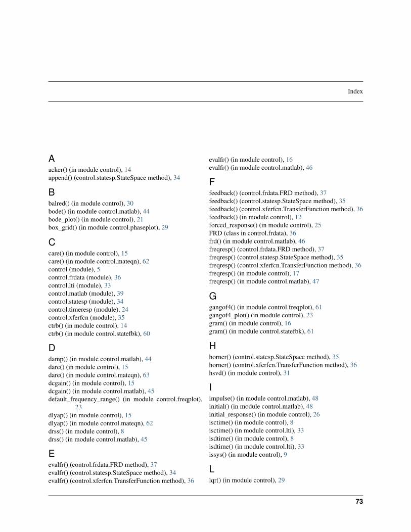
Index

Aacker() (in module control), 14append() (control.statesp.StateSpace method), 34

Bbalred() (in module control), 30bode() (in module control.matlab), 44bode_plot() (in module control), 21box_grid() (in module control.phaseplot), 29

Ccare() (in module control), 15care() (in module control.mateqn), 62control (module), 5control.frdata (module), 36control.lti (module), 33control.matlab (module), 39control.statesp (module), 34control.timeresp (module), 24control.xferfcn (module), 35ctrb() (in module control), 14ctrb() (in module control.statefbk), 60

Ddamp() (in module control.matlab), 44dare() (in module control), 15dare() (in module control.mateqn), 63dcgain() (in module control), 15dcgain() (in module control.matlab), 45default_frequency_range() (in module control.freqplot),

23dlyap() (in module control), 15dlyap() (in module control.mateqn), 62drss() (in module control), 8drss() (in module control.matlab), 45

Eevalfr() (control.frdata.FRD method), 37evalfr() (control.statesp.StateSpace method), 34evalfr() (control.xferfcn.TransferFunction method), 36

evalfr() (in module control), 16evalfr() (in module control.matlab), 46

Ffeedback() (control.frdata.FRD method), 37feedback() (control.statesp.StateSpace method), 35feedback() (control.xferfcn.TransferFunction method), 36feedback() (in module control), 12forced_response() (in module control), 25FRD (class in control.frdata), 36frd() (in module control.matlab), 46freqresp() (control.frdata.FRD method), 37freqresp() (control.statesp.StateSpace method), 35freqresp() (control.xferfcn.TransferFunction method), 36freqresp() (in module control), 17freqresp() (in module control.matlab), 47

Ggangof4() (in module control.freqplot), 61gangof4_plot() (in module control), 23gram() (in module control), 16gram() (in module control.statefbk), 61

Hhorner() (control.statesp.StateSpace method), 35horner() (control.xferfcn.TransferFunction method), 36hsvd() (in module control), 31

Iimpulse() (in module control.matlab), 48initial() (in module control.matlab), 48initial_response() (in module control), 26isctime() (in module control), 8isctime() (in module control.lti), 33isdtime() (in module control), 8isdtime() (in module control.lti), 33issys() (in module control), 9

Llqr() (in module control), 29

73


lqr() (in module control.statefbk), 59lsim() (in module control.matlab), 49Lti (class in control.lti), 33lyap() (in module control), 17lyap() (in module control.mateqn), 62

Mmargin() (in module control), 18margin() (in module control.matlab), 50markov() (in module control), 19minreal() (control.statesp.StateSpace method), 35minreal() (control.xferfcn.TransferFunction method), 36modred() (in module control), 31

Nnegate() (in module control), 13ngrid() (in module control.matlab), 51nichols() (in module control.nichols), 59nichols_plot() (in module control), 23nyquist() (in module control.freqplot), 58nyquist_plot() (in module control), 22

Oobsv() (in module control), 19obsv() (in module control.statefbk), 60

Ppade() (in module control), 9pade() (in module control.delay), 61parallel() (in module control), 13phase_crossover_frequencies() (in module control), 19phase_plot() (in module control.phaseplot), 28place() (in module control), 30place() (in module control.statefbk), 59pole() (control.statesp.StateSpace method), 35pole() (control.xferfcn.TransferFunction method), 36pole() (in module control), 20pole() (in module control.matlab), 51pzmap() (in module control.pzmap), 58

RreturnScipySignalLti() (control.statesp.StateSpace

method), 35returnScipySignalLti() (control.xferfcn.TransferFunction

method), 36rlocus() (in module control.matlab), 51root_locus() (in module control), 20rss() (in module control.matlab), 52

Ssample_system() (in module control), 9series() (in module control), 13ss() (in module control), 5

ss() (in module control.matlab), 52ss2tf() (in module control), 10ss2tf() (in module control.matlab), 53ssdata() (in module control), 10ssdata() (in module control.matlab), 54stability_margins() (in module control), 20StateSpace (class in control), 5StateSpace (class in control.statesp), 34step() (in module control.matlab), 54step_response() (in module control), 27

Ttf() (in module control), 7tf() (in module control.matlab), 55tf2ss() (in module control), 11tf2ss() (in module control.matlab), 56tfdata() (in module control), 11tfdata() (in module control.matlab), 57timebase() (in module control), 12timebase() (in module control.lti), 34timebaseEqual() (in module control), 12timebaseEqual() (in module control.lti), 34TransferFunction (class in control), 6TransferFunction (class in control.xferfcn), 35

Uunwrap() (in module control), 32unwrap() (in module control.ctrlutil), 62

Zzero() (control.statesp.StateSpace method), 35zero() (control.xferfcn.TransferFunction method), 36zero() (in module control), 21zero() (in module control.matlab), 57

74 Index

Documents

Python Control Documentation - Read the Docs · Welcome to the Python Control Systems Library (python-control) User’s Manual. This manual describes the python- control package,