Q = CV C R V - Princeton Universitywbialek/intsci_web/dynamics1.5.pdf · Problem 20: In the previous paragraph we made some claims about the behavior of x(t), based on Eq (1.179),

1.5. SIMPLE CIRCUITS AND POPULATION DYNAMICS 73

C R VQ = CV

I = V/R1

Figure 1.16: A capacitor C and resistor R connected in parallel. The voltage drop V isthe same across the two elements of the circuit, while the currents flowing through thetwo circuit element must add to zero, as expressed in Eq (1.165).

1.5 Simple circuits and population dynamics

Most of you remember a little bit about electrical circuits from your highschool physics classes. In Fig 1.16 we show a capacitor C and a resistor Rconnected in parallel. Here “parallel” means that the voltage di!erence Vbetween the two plates of the capacitor is the same as the voltage di!erenceacross the resistor. In this simple case the circuit is closed and there is nopath for current to flow out, so the current that flows through the capacitorand resistor must add up to zero. This condition of zero current (an appli-cation of Kircho!’s laws, if that jogs your memory) allows us to write downthe equation for the dynamics of the voltage V in this circuit.

Recall that the current which flows through the resistor is just I1 = V/R.We usually think of the capacitor as being described by Q = CV , where Qis the charge on the capacitor plates, but of course if the charge changeswith time there is a current flow (by definition), so that the current which

74 CHAPTER 1. NEWTON’S LAWS, CHEMICAL KINETICS, ...

flows through the capacitor is I2 = d(CV )/dt = C(dV/dt). Adding thesecurrents must give zero, and this must be true at every moment of time t:

I1 + I2 =V (t)R

+ CdV (t)

dt= 0. (1.165)

It is slightly more convenient to write this as

RCdV (t)

dt+ V (t) = 0. (1.166)

We recognize Eq (1.166) as the same equation we have seen before, bothin the mechanics of motion with drag and in first order chemical kinetics.By now we know that the solution is an exponential decay,

V (t) = V (0)e!t/! , (1.167)

where the time constant ! = RC. As you might guess by looking at thecircuit—there is no battery and no current source—any initial voltage V (0)decays to zero, and this decay happens on a time scale ! = RC. This isimportant because most circuits that we build, including the circuits on thechips in your computer, have some combination of resistance and capaci-tance, and so we know that there is a time scale over which these circuitswill lose their memory. In memory chips we want this to be a very long time,so (roughly speaking) one tries to design the circuit so that R is very large.Conversely, on the processor chips things should happen fast, so RC shouldbe small. You may recall that the capacitance C is determined largely bygeometry—how big are the plates and how far apart are they?—so if wewant to squeeze a certain number of circuit elements into a given area of thechip the capacitances are more or less fixed, and the challenge is to reduceR.

Almost the same equations arise in a very di!erent context, namelypopulation growth. Imagine that we put a small number of bacteria intoa large container, with plenty of food; you will soon do more or less thisexperiment in the lab part of the course. Let’s call n(t) the number ofbacteria present at time t. Because the bacteria divide, n(t) increases. As afirst approximation, it’s plausible that the rate at which new bacteria appearis proportional to the number of bacteria already there, so we can write

dn(t)dt

= rn(t), (1.168)

where r is the “growth rate.” This is just like the equations we have seenso far, but the sign is di!erent.


When we had an equation of the form

dx

dt= !kx, (1.169)

we found that the solution is of the form x(t) = A exp(!kt), where theconstant A = x(t = 0). More generally we can say that this solution is ofthe form x(t) = A exp("t), and it turns out the " = !k. As will becomeclearer in the next few lectures, this exponential form is very general, andhelps us solve a large class of problems. So, let’s try it here.

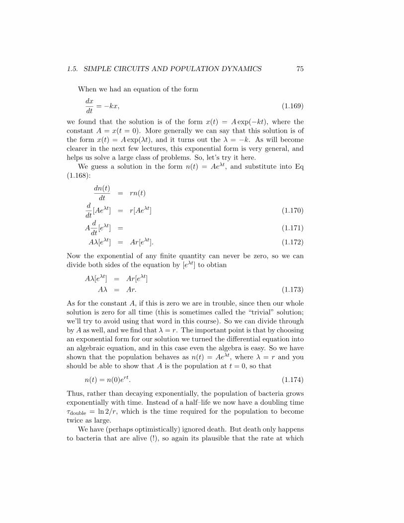
We guess a solution in the form n(t) = Ae"t, and substitute into Eq(1.168):

dn(t)dt

= rn(t)

d

dt[Ae"t] = r[Ae"t] (1.170)

Ad

dt[e"t] = (1.171)

A"[e"t] = Ar[e"t]. (1.172)

Now the exponential of any finite quantity can never be zero, so we candivide both sides of the equation by [e"t] to obtian

A"[e"t] = Ar[e"t]A" = Ar. (1.173)

As for the constant A, if this is zero we are in trouble, since then our wholesolution is zero for all time (this is sometimes called the “trivial” solution;we’ll try to avoid using that word in this course). So we can divide throughby A as well, and we find that " = r. The important point is that by choosingan exponential form for our solution we turned the di!erential equation intoan algebraic equation, and in this case even the algebra is easy. So we haveshown that the population behaves as n(t) = Ae"t, where " = r and youshould be able to show that A is the population at t = 0, so that

n(t) = n(0)ert. (1.174)

Thus, rather than decaying exponentially, the population of bacteria growsexponentially with time. Instead of a half–life we now have a doubling time!double = ln 2/r, which is the time required for the population to becometwice as large.

We have (perhaps optimistically) ignored death. But death only happensto bacteria that are alive (!), so again its plausible that the rate at which


the population decreases by death is proportional to the number of bacteria,!dn(t), where d is the death rate. Then

dn(t)dt

= rn(t)! dn(t) = (r ! d)n(t), (1.175)

so if we define a new growth rate r" = r ! d everything is as it was before.In fact, if we are just watching the total number of bacteria we can’t tell thedi!erence between a slower growth rate and a faster death rate.

These equations for the population of bacteria are approximate. Let’smake a list of some of the things that we have ignored, and see if we canimprove our approximation:

• We’ve assumed that the discreteness of bacteria isn’t important—youcan’t have 305.7 bacteria, but we pretend that n(t) is a continuousfunction. Probably this isn’t too bad if the population is of a reason-able size.

• We’ve assumed that all the bacteria are the same. It’s not so hard tomake sure that they are genetically identical—just start with one anddon’t let things run long enough to accumulate too many mutations.It takes more e!ort to insure that all the bacteria experience the sameenvironment.

• We’ve assumed that the bacteria don’t murder each other, and moregently that the consumption of food by the ever increasing number ofbacteria doesn’t limit the growth.

• We’ve assumed that the growth isn’t synchronized.

These last two points deserve some discussion.We can model the “environmental impact” of the bacteria by saying

that the e!ective growth rate r" gets smaller as the number of bacteriagets larger. Certainly this starts out being linear, so maybe we can writer" = r0[1! an(t)], so that

dn(t)dt

= r0[1! an(t)]n(t). (1.176)

But then this defines a critical population size nc = 1/a such that oncen = nc the growth will stop (dn/dt = 0)—the environment has reached itscapacity for sustaining the population. It’s natural to measure the popu-lation size as a fraction of this capacity, so we write x = n/nc, so (being


careful with all the steps, since this is the kind of thing you’ll need to domany times)

dn(t)dt

= r0[1! an(t)]n(t)

d

dt

!nc

n(t)nc

"= r0

#1! a

!nc

n(t)nc

"$ !nc

n(t)nc

"

(1.177)

ncdx(t)

dt= [1! (anc)x(t)]ncx(t) (1.178)

dx(t)dt

= r0x(t)[1! x(t)], (1.179)

where at the last step we cancel the common factor of nc and use the factthat (by our choice of nc) anc = 1.

This equation predicts that if we start with a very small (x" 1) popu-lation, the growth will be exponential with a rate r0, but as x gets close to1 this has to stop, and the population will reach a steady, saturated state.These dynamics will be important in your experiments, so let’s actually solvethis equation.

Problem 20: In the previous paragraph we made some claims about the behavior ofx(t), based on Eq (1.179), but without actually solving the equation (yet). Can you explainwhy these claims are true, also without constructing a full solution? To get started, canyou make a simpler, approximate equation that should describe the dynamics accuratelywhen x! 1?

We use the same idea as before, “moving” the x’s to one side of theequation and the dt to the other:

dx

dt= r0x[1! x] (1.180)

dx

x(1! x)= r0dt. (1.181)

If you remember how to do the integral%

dx

x(1! x),


you can proceed directly from here. If, like me, you remember that%

dx

x= lnx,

but aren’t sure what to do about the more complicated case, then you needto turn the problem you have into the one you remember how to solve.

Problem 21: Starting with

Zdxx

= ln x, (1.182)

remind yourself of why

Zdx

1" x= " ln(1" x). (1.183)

The trick we need here is that fractions which have products in thedenominator can be expanded so that they just have single terms in thedenominator. What this means is that we want to try writing

1x(1! x)

=A

x+

B

1! x, (1.184)

but we have to choose A and B correctly. The way to do this is to workbackwards:

A

x+

B

1! x=

A(1! x)x(1! x)

+Bx

x(1! x)(1.185)

=A(1! x) + Bx

x(1! x)(1.186)

=A + (B !A)x

x(1! x). (1.187)

Now it is clear that if we want this to equal

1x(1! x)

,


then we have to choose A = 1 and B = A = 1. So we have

1x(1! x)

=1x

+1

1! x, (1.188)

and now we can go back to solving our original problem:

dx

x(1! x)= r0dt

dx

x+

dx

1! x= r0dt (1.189)

% x(t)

x(0)

dx

x+

% x(t)

x(0)

dx

1! x=

% t

0r0dt (1.190)

ln(x)

&&&&&

x(t)

x(0)

! ln(1! x)

&&&&&

x(t)

x(0)

= r0t (1.191)

ln[x(t)]! ln[x(0)]! ln[1! x(t)] + ln[1! x(0)] = r0t (1.192)

ln#

x(t)x(0)

· 1! x(0)1! x(t)

$= r0t (1.193)

x(t)x(0)

· 1! x(0)1! x(t)

= exp(r0t) (1.194)

x(t)1! x(t)

=x(0)

1! x(0)exp(r0t).

(1.195)

Note that in the last steps we use the fact that sums (di!erences) of logs arethe logs or products (ratios), and then we get rid of the logs by exponentiat-ing both sides of the equation. The very last step puts the time dependentx(t) on left side and the initial condition on the right.

Equation (1.195) is almost what we want, but it would be more usefulto write x(t) explicitly. Notice that what we have is of the form

x(t)1! x(t)

= F, (1.196)

where F is some factor. You’ll see things like this again, so it might beworth knowing the trick, which is to invert both sides, rearrange, and invert


again:

x(t)1! x(t)

= F

1! x(t)x(t)

=1F

(1.197)

1x(t)

! 1 = (1.198)

1x(t)

= 1 +1F

(1.199)

=F + 1

F(1.200)

x(t) =F

1 + F. (1.201)

Armed with this little bit of algebra, we can solve for x(t) in Eq (1.195):

x(t)1! x(t)

=x(0)

1! x(0)exp(r0t)

# x(t) =x(0)

1!x(0) exp(r0t)

1 + x(0)1!x(0) exp(r0t)

(1.202)

=x(0) exp(r0t)

[1! x(0)] + x(0) exp(r0t), (1.203)

where the last step is just to make things look a little nicer.Some graphs of Eq (1.203) are shown in Fig 1.17. You should notice that

all of the curves run smoothly from x(0) up to the maximum value of x = 1at long times. Indeed, all the curves seem to look the same, just shiftedalong the time axis. Hopefully you’ll something like this in the lab!

Problem 22: It’s useful to look at a expression like Eq (1.203) and “see” some ofthe key features that appear in the graphs, without actually making the exact plots.

(a.) Be sure that if you evaluate x(t) at t = 0 you really do get x(0), as you should ifwe did all the manipulations correctly.

(b.) Ask yourself what happens as t # $. You should be able to see that x(t)approaches 1, no matter what the initial value x(0), as long as it’s not zero.

(c.) Show that you rewrite Eq (1.203) as

x(t) =1

1 + exp["r0(t" t0)], (1.204)


0 2 4 6 8 10 12 14 16 18 200

0.1

0.2

0.3

0.4

0.5

0.6

0.7

0.8

0.9

1

r0 t

norm

alize

d po

pula

tion

size

x(t)

x(0) = 0.1x(0) = 0.01x(0) = 0.001x(0) = 0.0001

Figure 1.17: Dynamics of population growth as predicted by Eq (1.203), the solution toEq (1.179). Time is measured in units of the growth rate r0 of small populations, and thepopulation size is normalized the “capacity” of the environment.

where t0 depends on the initial population. What does this mean about the growth curvesthat start with di!erent values of x(0)?

Problem 23: As discussed in connection with the first laboratory and in Section1.1, an object moving through a fluid at relatively high velocities experiences a drag forceproportional to the square of its velocity. In the presence gravity this means that F = macan be written as

mdvdt

= "av2 + mg, (1.205)

where the velocity v is positive if the object is moving downwards, a is the drag coe"cient,and g as usual is the acceleration due to gravity. As noted in the lectures, a similarequations can arise in chemical kinetics.

(a.) For any given system, the usual units of time, speed, etc. might not be verynatural. Perhaps there is some natural time scale t0 and a natural velocity scale v0 suchthat if we measure things in these units our equation will look simpler. Specifically,consider variables u % v/v0 and ! % t/t0. Show that by proper choice of t0 and v0 onecan make all the parameters (m, g, a) disappear from the di!erential equation for u(!).

(b.) Solve the di!erential equation for u(!). Does this function have a universalshape? Since we have gotten rid of all the parameters, is there anything left on whichthe shape could depend? If you need help doing an integral it’s OK to use a table (orperhaps an electronic equivalent), but you need to give references. Translate your resultsinto predictions about v(t).

(c.) Suppose that the initial velocity v(t = 0) is very close to the terminal velocityv! =

pmg/a. Show that your exact solution for v(t) is approximately an exponential


decay back to the terminal velocity. Then go back to Eq (1.205) and write v(t) = v! +"v(t), and make the approximation that "v is small, and hence "v2 is even smaller and canbe neglected. Can you now show that this approximate equation leads to an exponentialdecay of "v(t), in agreement with your exact solution?

(d.) Explain the similarities between this problem and the population growth problemthat starts with Eq (1.179) and leads to the results in Fig 1.17. Can you make an exactmapping from one problem to the other?

What about synchronization? Cell growth and division is a cycle, andif this cycle runs like a clock then we can imagine getting all the clocksaligned so that the population of bacteria holds fixed for some length oftime, then doubles as all the cells proceed complete their cycle, then holdsfixed, doubles again, and so on. In fact, real single celled organisms losetheir synchronization if they don’t communicate. On the other hand, manyorganisms (including big complicated ones not so di!erent from us) get syn-chronized by the seasons—we are all familiar with the nearly simultaneousappearance of all the baby birds at the same time of year. This suggests thatrather than writing down a di!erential equation, we should use one year asthe natural unit of time and ask how the number of organisms in one yearn(t) depends on the number that were there last year n(t! 1). Again if wejust think about growth we would argue that the number of new organismsif proportional to the number that we started with, hence

n(t) = Gn(t! 1), (1.206)

where G > 1 means that we are describing growth from season to seasonwhile G < 1 means that the population is dying out. It’s interesting that inthis case the seasonal synchronization doesn’t make any di!erence, becausethe solution still is exponential: n(t) = n(0)et/! , where ! = 1/(lnG).

Problem 24: Verify that Eq (1.206) is solved by n(t) = n(0)et/! , with ! = 1/(ln G).As a prelude to things which will be important in the next major section of the course,consider a population in which some fraction of the organisms wait for two seasons toreproduce, so that

n(t) = G1n(t" 1) + G2n(t" 2). (1.207)

Can you still find a solution of the form n(t) & et/!? If so, what is the equation thatdetermines the value of the time constant !?


600 620 640 660 680 700 720 740 760 780 8000

0.1

0.2

0.3

0.4

0.5

0.6

0.7

0.8

0.9

1

discrete time

popu

latio

n siz

e x(

t)

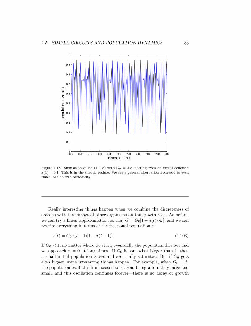
Figure 1.18: Simulation of Eq (1.208) with G0 = 3.8 starting from an initial conditonx(1) = 0.1. This is in the chaotic regime. We see a general alternation from odd to eventimes, but no true periodicity.

Really interesting things happen when we combine the discreteness ofseasons with the impact of other organisms on the growth rate. As before,we can try a linear approximation, so that G = G0[1!n(t)/nc], and we canrewrite everything in terms of the fractional population x:

x(t) = G0x(t! 1)[1! x(t! 1)]. (1.208)

If G0 < 1, no matter where we start, eventually the population dies out andwe approach x = 0 at long times. If G0 is somewhat bigger than 1, thena small initial population grows and eventually saturates. But if G0 getseven bigger, some interesting things happen. For example, when G0 = 3,the population oscillates from season to season, being alternately large andsmall, and this oscillation continues forever—there is no decay or growth


to a steady state. When G0 = 3.5, there is an oscillation with alternatingseasons of large and small population, but it takes a total of four seasonsbefore the population repeats exactly. We say that at G0 = 3 we observe a“period 2” oscillation, and at G0 = 3.5 we observe a “period 4” oscillation. Ifwe keep increasing G0 we can observe period 8, period 16, ... all the powersof 2 (!). The transitions to longer and longer periods come more quicklyas G0 increases, until we exceed a critical value of G0 and the trajectoriesx(t) start to look completely random, even though they are generated bythe simple Eq (1.208); see Fig 1.18.

Problem 25: Write a program to generate the trajectories x(t) that are predicted byEq (1.208). Run this program, exploring di!erent values of G0, and verify the statementsmade in the previous paragraph. In particular, try starting with di!erent initial conditionsx(0), and see whether the solutions are “attracted” to some simple for at long times, orwhether trajectories that start with slightly di!erent values of x(0) end up looking verydi!erent from each other. Does this dependence on initial conditions vary with the value ofG0? Can you see what this might have to do with the problem of predicting the weather?

The random looking trajectories of Fig 1.18 are called chaotic, andthe discovery that such simple deterministic equations can generate chaoschanged completely how we look at the dynamics of the world around us.What is remarkable is that the surprising properties of this simple equation(which you can rediscover for yourself even with a pocket calculator) areprovably the properties of a broad class of equations, and one can observethe sequence of period doublings and the resulting chaos in real physicalsystems, matching quantitatively the predictions of the simple model to keyfeatures of the data.

This has been a scant introduction to a rich and beautiful subject. Pleaseask for more references if you are intrigued.

1.6. THE COMPLEXITY OF DNA SEQUENCES 85

1.6 The complexity of DNA sequences

This section remains to be written. Current students should see the lessformal notes posted to blackboard.

Problem 26: The total genomic DNA of a newly-discovered species of newt contains1200 copies of a 2 kb repeated sequence, 300 copies of a 6 kb repeated sequence as well as3000 kb of single-copy DNA.

(a.) What will the “Cot curve” (i.e. plot of the fraction of DNA remaining single-stranded vs. C0t) look like? Be sure to label the axes, and indicate the fractional contri-bution of the di!erent kinds of DNA.

(b.) Devise a procedure to prepare reasonably pure samples of the three kinds ofDNA. Explain how you would calculate the times of annealing required for each step.


Documents

Q = CV C R V - Princeton Universitywbialek/intsci_web/dynamics1.5.pdf · Problem 20: In the previous paragraph we made some claims about the behavior of x(t), based on Eq (1.179),