Q-value Q a bus 1 ride bus 17 ride the magic tram cs221.stanford.edu/q CS221 / Autumn 2017 / Liang & Ermon 1 In in the previous lecture, you probably had some model of the world (how

Lecture 8: MDPs II

CS221 / Spring 2018 / Sadigh

Question

If you wanted to go from Orbisonia to Rockhill, how would you get there?

ride bus 1

ride bus 17

ride the magic tram

cs221.stanford.edu/q

CS221 / Spring 2018 / Sadigh 1

• In in the previous lecture, you probably had some model of the world (how far Mountain View is, how longbiking, driving, and Caltraining each take). But now, you should have no clue what’s going on. This isthe setting of reinforcement learning. Now, you just have to try things and learn from your experience- that’s life!

Review: MDPs

in in,stay

in,quit end

stay

(2/3): $4

(1/3): $4quit

1: $10

Definition: Markov decision process

States: the set of states

sstart ∈ States: starting state

Actions(s): possible actions from state s

T (s, a, s′): probability of s′ if take action a in state s

Reward(s, a, s′): reward for the transition (s, a, s′)

IsEnd(s): whether at end of game

0 ≤ γ ≤ 1: discount factor (default: 1)


• Last time, we talked about MDPs, which we can think of as graphs, where each node is either a state sor a chance node (s, a). Actions take us from states to chance nodes (which we choose), and transitionstake us from chance nodes to states (which nature chooses according to the transition probabilities).

Review: MDPs

• Following a policy π produces a path (episode)

s0; a1, r1, s1; a2, r2, s2; a3, r3, s3; . . . ; an, rn, sn

• Value function Vπ(s): expected utility if follow π from state s

Vπ(s) =

{0 if IsEnd(s)

Qπ(s, π(s)) otherwise.

• Q-value function Qπ(s, a): expected utility if first take action afrom state s and then follow π

Qπ(s, a) =∑s′ T (s, a, s

′)[Reward(s, a, s′) + γVπ(s′)]


• Given a policy π and an MDP, we can run the policy on the MDP yielding a sequence of states, action,rewards s0; a1, r1, s1; a2, r2, s2; . . . . Formally, for each time step t, at = π(st−1), and st is sampled withprobability T (st−1, at, st). We call such a sequence an episode (a path in the MDP graph). This will bea central notion in this lecture.

• Each episode (path) is associated with a utility, which is the discounted sum of rewards: u1 = r1 + γr2 +γ2r3 + · · · . It’s important to remember that the utility u1 is a random variable which depends on howthe transitions were sampled.

• The value of the policy (from state s0) is Vπ(s0) = E[u1], the expected utility. In the last lecture, weworked with the values directly without worrying about the underlying random variables (but that will soonno longer be the case). In particular, we defined recurrences relating the value Vπ(s) and Q-value Qπ(s, a),which represents the expected utility from starting at the corresponding nodes in the MDP graph.

• Given these mathematical recurrences, we produced algorithms: policy evaluation computes the value ofa policy, and value iteration computes the optimal policy.

Unknown transitions and rewards

Definition: Markov decision process

States: the set of states

sstart ∈ States: starting state

Actions(s): possible actions from state s

IsEnd(s): whether at end of game

0 ≤ γ ≤ 1: discount factor (default: 1)

reinforcement learning!


• In this lecture, we assume that we have an MDP where we neither know the transitions nor the rewardfunctions. We are still trying to maximize expected utility, but we are in a much more difficult settingcalled reinforcement learning.

Mystery game

Example: mystery buttons

For each round r = 1, 2, . . .• You choose A or B.

• You move to a new state and get some rewards.

Start A B

State: 5,0 Rewards: 0


• To put yourselves in the shoes of a reinforcement learner, try playing the game. You can either push theA button or the B button. Each of the two actions will take you a new state and give you some reward.

• This simple game illustrates some of the challenges of reinforcement learning: we should take good actionsto get rewards, but in order to know which actions are good, we need to explore and try different actions.

Roadmap

Reinforcement learning

Monte Carlo methods

Bootstrapping methods

Covering the unknown

Summary


From MDPs to reinforcement learning

Markov decision process (offline)

• Have mental model of how the worldworks.

• Find policy to collect maximum rewards.

Reinforcement learning (online)

• Don’t know how the world works.

• Perform actions in the world to find outand collect rewards.


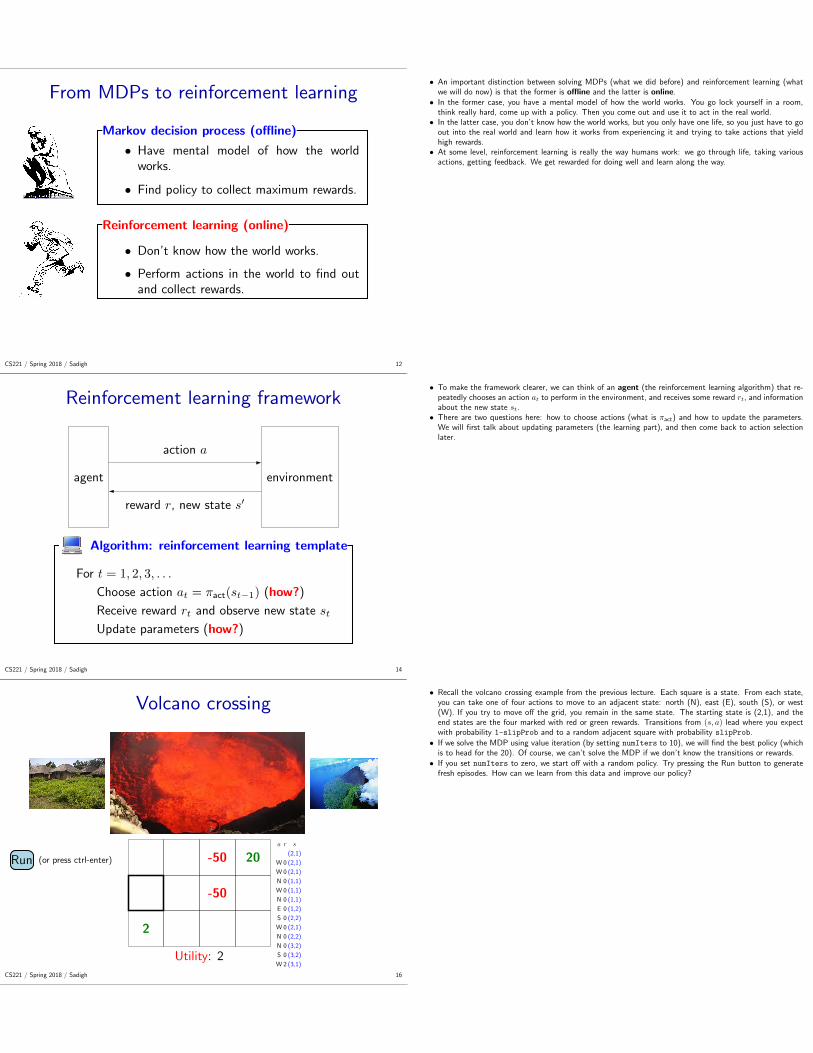
• An important distinction between solving MDPs (what we did before) and reinforcement learning (whatwe will do now) is that the former is offline and the latter is online.

• In the former case, you have a mental model of how the world works. You go lock yourself in a room,think really hard, come up with a policy. Then you come out and use it to act in the real world.

• In the latter case, you don’t know how the world works, but you only have one life, so you just have to goout into the real world and learn how it works from experiencing it and trying to take actions that yieldhigh rewards.

• At some level, reinforcement learning is really the way humans work: we go through life, taking variousactions, getting feedback. We get rewarded for doing well and learn along the way.

Reinforcement learning framework

agent environment

action a

reward r, new state s′

Algorithm: reinforcement learning template

For t = 1, 2, 3, . . .

Choose action at = πact(st−1) (how?)

Receive reward rt and observe new state st

Update parameters (how?)


• To make the framework clearer, we can think of an agent (the reinforcement learning algorithm) that re-peatedly chooses an action at to perform in the environment, and receives some reward rt, and informationabout the new state st.

• There are two questions here: how to choose actions (what is πact) and how to update the parameters.We will first talk about updating parameters (the learning part), and then come back to action selectionlater.

Volcano crossing

Run (or press ctrl-enter) -50 20

-50

2

Utility: 2

a r s

(2,1)

W 0 (2,1)

W 0 (2,1)

N 0 (1,1)

W 0 (1,1)

N 0 (1,1)

E 0 (1,2)

S 0 (2,2)

W 0 (2,1)

N 0 (2,2)

N 0 (3,2)

S 0 (3,2)

W 2 (3,1)


• Recall the volcano crossing example from the previous lecture. Each square is a state. From each state,you can take one of four actions to move to an adjacent state: north (N), east (E), south (S), or west(W). If you try to move off the grid, you remain in the same state. The starting state is (2,1), and theend states are the four marked with red or green rewards. Transitions from (s, a) lead where you expectwith probability 1-slipProb and to a random adjacent square with probability slipProb.

• If we solve the MDP using value iteration (by setting numIters to 10), we will find the best policy (whichis to head for the 20). Of course, we can’t solve the MDP if we don’t know the transitions or rewards.

• If you set numIters to zero, we start off with a random policy. Try pressing the Run button to generatefresh episodes. How can we learn from this data and improve our policy?

Roadmap


Monte Carlo methods



Summary


Model-based Monte Carlo

Data: s0; a1, r1, s1; a2, r2, s2; a3, r3, s3; . . . ; an, rn, sn

Key idea: model-based learning

Estimate the MDP: T (s, a, s′) and Reward(s, a, s′)

Transitions:

T̂ (s, a, s′) = # times (s, a, s′) occurs# times (s, a) occurs

Rewards:

R̂eward(s, a, s′) = average of r in (s, a, r, s′)


Model-based Monte Carlo

Example: model-based Monte Carlo

Data (following policy π):

S1; A, 3, S2; B, 0, S1; A, 5, S1; A, 7, S1

Estimates:

T̂ (S1,A,S1) = 23

T̂ (S1,A,S2) = 13

R̂eward(S1,A,S1) = 12 (5 + 7) = 6

R̂eward(S1,A,S2) = 3

Estimates converge to true values (under certain conditions)


• The first idea is called model-based Monte Carlo, where we try to estimate the model (transitions andrewards) using Monte Carlo simulation.

• Note: if the rewards are deterministic, then every time we see a (s, a, s′) triple, we get the same numberso taking the average just returns that number; allowing averages allows us to handle non-deterministic

rewards, in which case R̂eward(s, a, s′) would converge to its expectation.• Monte Carlo is a standard way to estimate the expectation of a random variable by taking an average over

samples of that random variable.• Here, the data used to estimate the model is the sequence of states, actions, and rewards in the episode.

Note that the samples being averaged are not independent (because they come from the same episode), butthey do come from a Markov chain, so it can be shown that these estimates converge to the expectationsby the ergodic theorem (a generalization of the law of large numbers for Markov chains).

• But there is one important caveat...

Problem


S1; A, 3, S2; B, 0, S1; A, 5, S1; A, 7, S1

Problem: won’t even see (s, a) if a 6= π(s)

Key idea: exploration

To do reinforcement learning, need to explore the state space.

Solution: need π to explore explicitly (more on this later)


• So far, our policies have been deterministic, mapping s always to π(s). However, if we use such a policyto generate our data, there are certain (s, a) pairs that we will never see and therefore never be able toestimate their Q-value and never know what the effect of those actions are.

• This problem points at the most important characteristic of reinforcement learning, which is the need forexploration. This distinguishes reinforcement learning from supervised learning, because now we actuallyhave to act to get data, rather than just having data poured over us.

• To close off this point, we remark that if π is a non-deterministic policy which allows us to explore eachstate and action infinitely often (possibly over multiple episodes), then the estimates of the transitions andrewards will converge.

• Once we get an estimate for the transitions and rewards, we can simply plug them into our MDP and solveit using standard value or policy iteration to produce a policy.

• Notation: we put hats on quantities that are estimated from data (Q̂opt, T̂ ) to distinguish from the truequantities (Qopt, T ).

From model-based to model-free

Q̂opt(s, a) =∑s′

T̂ (s, a, s′)[R̂eward(s, a, s′) + γV̂opt(s′)]

All that matters for prediction is (estimate of) Qopt(s, a).

Key idea: model-free learning

Try to estimate Qopt(s, a) directly.


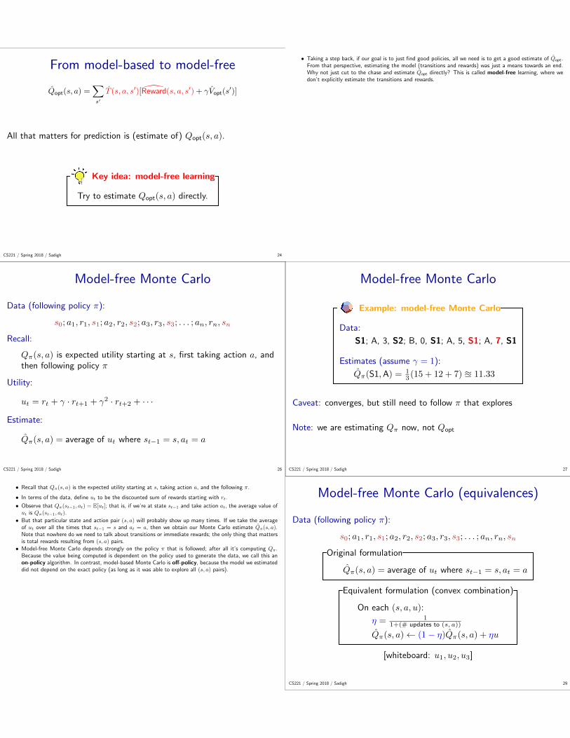
• Taking a step back, if our goal is to just find good policies, all we need is to get a good estimate of Q̂opt.From that perspective, estimating the model (transitions and rewards) was just a means towards an end.Why not just cut to the chase and estimate Q̂opt directly? This is called model-free learning, where wedon’t explicitly estimate the transitions and rewards.

Model-free Monte Carlo



Recall:

Qπ(s, a) is expected utility starting at s, first taking action a, andthen following policy π

Utility:

ut = rt + γ · rt+1 + γ2 · rt+2 + · · ·

Estimate:

Q̂π(s, a) = average of ut where st−1 = s, at = a


Model-free Monte Carlo

Example: model-free Monte Carlo

Data:

S1; A, 3, S2; B, 0, S1; A, 5, S1; A, 7, S1

Estimates (assume γ = 1):

Q̂π(S1,A) =13 (15 + 12 + 7) u 11.33

Caveat: converges, but still need to follow π that explores

Note: we are estimating Qπ now, not Qopt


• Recall that Qπ(s, a) is the expected utility starting at s, taking action a, and the following π.

• In terms of the data, define ut to be the discounted sum of rewards starting with rt.

• Observe that Qπ(st−1, at) = E[ut]; that is, if we’re at state st−1 and take action at, the average value ofut is Qπ(st−1, at).

• But that particular state and action pair (s, a) will probably show up many times. If we take the averageof ut over all the times that st−1 = s and at = a, then we obtain our Monte Carlo estimate Q̂π(s, a).Note that nowhere do we need to talk about transitions or immediate rewards; the only thing that mattersis total rewards resulting from (s, a) pairs.

• Model-free Monte Carlo depends strongly on the policy π that is followed; after all it’s computing Qπ.Because the value being computed is dependent on the policy used to generate the data, we call this anon-policy algorithm. In contrast, model-based Monte Carlo is off-policy, because the model we estimateddid not depend on the exact policy (as long as it was able to explore all (s, a) pairs).

Model-free Monte Carlo (equivalences)



Original formulation

Q̂π(s, a) = average of ut where st−1 = s, at = a

Equivalent formulation (convex combination)

On each (s, a, u):

η = 11+(# updates to (s, a))

Q̂π(s, a)← (1− η)Q̂π(s, a) + ηu

[whiteboard: u1, u2, u3]


• Over the next few slides, we will interpret model-free Monte Carlo in several ways. This is the samealgorithm, just viewed from different perspectives. This will give us some more intuition and allow us todevelop other algorithms later.

• The first interpretation is thinking in terms of interpolation. Instead of thinking of averaging as a batchoperation that takes a list of numbers (realizations of ut) and computes the mean, we can view it as aniterative procedure for building the mean as new numbers are coming in.

• In particular, it’s easy to work out for a small example that averaging is equivalent to just interpolatingbetween the old value Q̂π(s, a) (current estimate) and the new value u (data). The interpolation ratio ηis set carefully so that u contributes exactly the right amount to the average.

• But we could use a different choice of η. In practice, it is useful to set η to something that doesn’t decay asquickly (for example, η = 1/

√# updates to (s, a)) so that newer examples are favored. The motivation

is that as learning proceeds, later samples ut will be more reliable than earlier ones.

Model-free Monte Carlo (equivalences)

Equivalent formulation (convex combination)

On each (s, a, u):

Q̂π(s, a)← (1− η)Q̂π(s, a) + ηu

Equivalent formulation (stochastic gradient)

On each (s, a, u):

Q̂π(s, a)← Q̂π(s, a)− η[Q̂π(s, a)︸︷︷︸prediction

− u︸︷︷︸target

]

Implied objective: least squares regression

(Q̂π(s, a)− u)2


• The second equivalent formulation is making the update look like a stochastic gradient update. Indeed,if think about each (s, a, u) triple as an example (where (s, a) is the input and u is the output), thenthe model-free Monte Carlo is just performing stochastic gradient descent on a least squares regressionproblem, where the weight vector is Q̂π (which has dimensionality SA) and there is one feature template”(s, a) equals ”.

• The stochastic gradient descent view will become particularly relevant when we use non-trivial features on(s, a).

Volcanic model-free Monte Carlo

Run (or press ctrl-enter)

0

1

01

0

0

00 -50 20

1

1

10

0

0

01 -500

0

00

20

0

00

0

0

00

0

0

00

Utility: 2

a r s

(2,1)

N 0 (1,1)

W 0 (1,1)

S 0 (2,1)

E 0 (2,2)

W 0 (2,1)

S 2 (3,1)


• Let’s run model-free Monte Carlo on the volcano crossing example. slipProb is zero to make thingssimpler. We are showing the Q-values: for each state, we have four values, one for each action.

• Here, our exploration policy is one that chooses an action uniformly at random.

• Try pressing ”Run” multiple times to understand how the Q-values are set.

• Then try increasing numEpisodes, and seeing how the Q-values of this policy become more accurate.

• You will notice that a random policy has a very hard time reaching the 20.

Roadmap


Monte Carlo methods



Summary


SARSA



Algorithm: model-free Monte Carlo updates

When receive (s, a, u):

Q̂π(s, a)← (1− η)Q̂π(s, a) + η u︸︷︷︸data

Algorithm: SARSA

When receive (s, a, r, s′, a′):

Q̂π(s, a)← (1− η)Q̂π(s, a) + η[ r︸︷︷︸data

+γ Q̂π(s′, a′)︸︷︷︸

estimate

]


• Broadly speaking, reinforcement learning algorithms interpolate between new data (which specifies thetarget value) and the old estimate of the value (the prediction).

• Model-free Monte Carlo’s target was u, the discounted sum of rewards after taking an action. However,u itself is just an estimate of Qπ(s, a). If the episode is long, u will be a pretty lousy estimate. Thisis because u only corresponds to one episode out of a mind-blowing exponential (in the episode length)number of possible episodes, so as the epsiode lengthens, it becomes an increasingly less representativesample of what could happen. Can we produce better estimate of Qπ(s, a)?

• An alternative to model-free Monte Carlo is SARSA, whose target is r+γQ̂π(s, a). Importantly, SARSA’starget is a combination of the data (the first step) and the estimate (for the rest of the steps). In contrast,model-free Monte Carlo’s u is taken purely from the data.

Comparison


Key idea: bootstrapping

SARSA uses estimate Q̂π(s, a) instead of just raw data u.

• u is only based on one path, so could have large variance, need towait until end

• Q̂π(s′, a′) based on estimate, which is more stable, update imme-

diately


• The main advantage that SARSA offers over model-free Monte Carlo is that we don’t have to wait untilthe end of the episode to update the Q-value.

• If the estimates are already pretty good, then SARSA will be more reliable since u is based on only onepath whereas Q̂π(s

′, a′) is based on all the ones that the learner has seen before.

• Advanced: We can actually interpolate between model-free Monte Carlo (all rewards) and SARSA (onereward). For example, we could update towards rt + γrt+1 + γ2Q̂π(st+1, at+2) (two rewards). We caneven combine all of these updates, which results in an algorithm called SARSA(λ), where λ determinesthe relative weighting of these targets. See the Sutton/Barto reinforcement learning book (chapter 7) foran excellent introduction.

• Advanced: There is also a version of these algorithms that estimates the value function Vπ instead of Qπ.Value functions aren’t enough to choose actions unless you actually know the transitions and rewards.Nonetheless, these are useful in game playing where we actually know the transition and rewards, but thestate space is just too large to compute the value function exactly.

Question

Which of the following algorithms allows you to estimate Qopt(s, a) (se-lect all that apply)?

model-based Monte Carlo

model-free Monte Carlo

SARSA

cs221.stanford.edu/q


• Model-based Monte Carlo estimates the transitions and rewards, which fully specifies the MDP. With theMDP, you can estimate anything you want, including computing Qopt(s, a)

• Model-free Monte Carlo and SARSA are on-policy algorithms, so they only give you Q̂π(s, a), which isspecific to a policy π. These will not provide direct estimates of Qopt(s, a).

Q-learning

Problem: model-free Monte Carlo and SARSA only estimate Qπ, butwant Qopt to act optimally

Output MDP reinforcement learning

Qπ policy evaluation model-free Monte Carlo, SARSA

Qopt value iteration Q-learning


• Recall our goal is to get an optimal policy, which means estimating Qopt.

• The situation is as follows: Our two methods (model-free Monte Carlo and SARSA) are model-free, butonly produce estimates Qπ. We have one algorithm, model-based Monte Carlo, which can be used toproduce estimates of Qopt, but is model-based. Can we get an estimate of Qopt in a model-free manner?

• The answer is yes, and Q-learning is an off-policy algorithm that accomplishes this.

• One can draw an analogy between reinforcement learning algorithms and the classic MDP algorithms.MDP algorithms are offline, RL algorithms are online. In both cases, algorithms either output the Q-valuesfor a fixed policy or the optimal Q-values.

Q-learning

MDP recurrence:

Qopt(s, a) =∑s′

T (s, a, s′)[Reward(s, a, s′) + γVopt(s′)]

Algorithm: Q-learning [Watkins/Dayan, 1992]

On each (s, a, r, s′):

Q̂opt(s, a)← (1− η)Q̂opt(s, a)︸︷︷︸prediction

+ η(r + γV̂opt(s′))︸︷︷︸

target

]

Recall: V̂opt(s′) = max

a′∈Actions(s′)Q̂opt(s

′, a′)


• To derive Q-learning, it is instructive to look back at the MDP recurrence for Qopt. There are severalchanges that take us from the MDP recurrence to Q-learning. First, we don’t have an expectation overs′, but only have one sample s′.

• Second, because of this, we don’t want to just replace Q̂opt(s, a) with the target value, but want tointerpolate between the old value (prediction) and the new value (target).

• Third, we replace the actual reward Reward(s, a, s′) with the observed reward r (when the reward functionis deterministic, the two are the same).

• Finally, we replace Vopt(s′) with our current estimate V̂opt(s

′).

• Importantly, the estimated optimal value V̂opt(s′) involves a maximum over actions rather than taking the

action of the policy. This max over a′ rather than taking the a′ based on the current policy is the principledifference between Q-learning and SARSA.

Volcanic SARSA and Q-learning


0

0

00

0

0

00 -50 20

0

1

00

0

0

00 -500

0

00

20

0

00

0

0

00

0

0

00

Utility: 2

a r s

(2,1)

S 2 (3,1)


• Let us try SARSA and Q-learning on the volcanic example.

• If you increase numEpisodes to 1000, SARSA will behave very much like model-free Monte Carlo, com-puting the value of the random policy.

• However, note that Q-learning is computing an estimate of Qopt(s, a), so the resulting Q-values will bevery different. The average utility will not change since we are still following and being evaluated on thesame random policy. This is an important point for off-policy methods: the online performance (averageutility) is generally a lot worse and not representative of what the model has learned, which is captured inthe estimated Q-values.

Roadmap


Monte Carlo methods



Summary


Exploration

Algorithm: reinforcement learning template

For t = 1, 2, 3, . . .

Choose action at = πact(st−1) (how?)

Receive reward rt and observe new state st

Update parameters (how?)


Which exploration policy πact to use?


• We have so far given many algorithms for updating parameters (i.e., Q̂π(s, a) or Q̂opt(s, a)). If we weredoing supervised learning, we’d be done, but in reinforcement learning, we need to actually determine ourexploration policy πact to collect data for learning. Recall that we need to somehow make sure we getinformation about each (s, a).

• We will discuss two complementary ways to get this information: (i) explicitly explore (s, a) or (ii) explore(s, a) implicitly by actually exploring (s′, a′) with similar features and generalizing.

• These two ideas apply to many RL algorithms, but let us specialize to Q-learning.

No exploration, all exploitation

Attempt 1: Set πact(s) = arg maxa∈Actions(s)

Q̂opt(s, a)


0

0

00

0

0.3

00 -50 100

0

0

20

0.1

2

-250 -500

0

00

20

0.5

02

0

0

00

0

0

00

Average utility: 1.95

a r s

(2,1)

E 0 (2,2)

S 0 (3,2)

W 2 (3,1)

Problem: Q̂opt(s, a) estimates are inaccurate, too greedy!


• The naive solution is to explore using the optimal policy according to the estimated Q-value Q̂opt(s, a).

• But this fails horribly. In the example, once the agent discovers that there is a reward of 2 to be gottenby going south that becomes its optimal policy and it will not try any other action. The problem is thatthe agent is being too greedy.

• In the demo, if multiple actions have the same maximum Q-value, we choose randomly. Try clicking ”Run”a few times, and you’ll end up with minor variations.

• Even if you increase numEpisodes to 10000, nothing new gets learned.

No exploitation, all exploration

Attempt 2: Set πact(s) = random from Actions(s)


98.4

98.4

98.498.4

98.4

98.4

-5098.4 -50 100

98.4

2

98.498.4

98.4

98.4

-5098.4 -5099.2

77.5

96.2-49.6

298.4

98.4

98.42

-50

97.8

98.498.1

98.7

97.9

98.198

Average utility: -19.15

a r s

(2,1)

S 2 (3,1)

Problem: average utility is low because exploration is not guided


• We can go to the other extreme and use an exploration policy that always chooses a random action. Itwill do a much better job of exploration, but it doesn’t exploit what it learns and ends up with a very lowutility.

• It is interesting to note that the value (average over utilities across all the episodes) can be quite smalland yet the Q-values can be quite accurate. Recall that this is possible because Q-learning is an off-policyalgorithm.

Exploration/exploitation tradeoff

Key idea: balance

Need to balance exploration and exploitation.

Examples from life: restaurants, routes, research


Epsilon-greedy

Algorithm: epsilon-greedy policy

πact(s) =

{argmaxa∈Actions Q̂opt(s, a) probability 1− ε,

random from Actions(s) probability ε.


99.8

100

100100

99.6

100

-50100 -50 100

100

2

100100

100

100

-50100 -50100

100

100-50

2100

100

1002

-50

100

100100

100

100

100100


a r s

(2,1)

W 0 (2,1)

N 0 (1,1)

S 0 (2,1)

W 0 (2,1)

W 0 (2,1)

E 0 (2,2)

S 0 (3,2)

E 0 (3,3)

E 0 (3,4)

N 0 (2,4)

N 100 (1,4)


• The natural thing to do when you have two extremes is to interpolate between the two. The result is theepsilon-greedy algorithm which explores with probability ε and exploits with probability 1− ε.

• Over time, it is natural to let ε decrease over time. When you’re young, you want to explore a lot (ε = 1).After a certain point, when you feel like you’ve seen all there is to see, then you start exploiting (ε = 0).

• For example, we let ε = 1 for the first third of the episodes, ε = 0.5 for the second third, and ε = 0 forthe final third. This is not the optimal schedule. Try playing around with other schedules to see if you cando better.

Generalization

Problem: large state spaces, hard to explore

1.2

2

1.50

0

1.9

11

0

1.5

00

0

0.5

00

0

0

-250 -50 20

1.9

1.9

21.6

1.8

2

1.82

0

1

0.82

0.3

1

01

0

0

00 -500

0

00

2

2

22

2

1.9

1.82

1.9

0.9

0.51.9

0.3

0

01.5

0

0

-250 -500

0

00

2

2

22

1.6

1.1

1.52

1.7

1

01.5

0

0

00

0

0

-250 -500

0

00

20

1.4

0.71.9

0

0

01.6

0

0

00

0

0

00

0

0

00

0

0

00


a r s

(3,1)

S 0 (4,1)

S 2 (5,1)


• Now we turn to another problem with vanilla Q-learning.

• In real applications, there can be millions of states, in which there’s no hope for epsilon-greedy to exploreeverything in a reasonable amount of time.

Q-learning

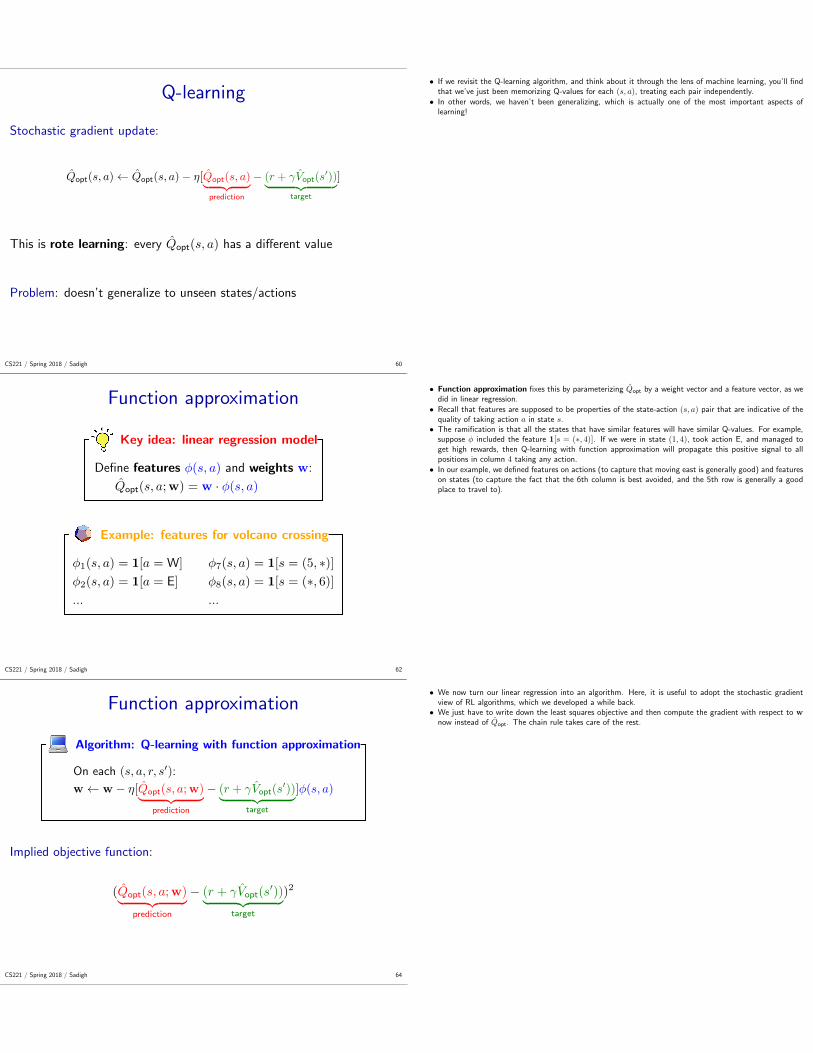
Stochastic gradient update:

Q̂opt(s, a)← Q̂opt(s, a)− η[Q̂opt(s, a)︸︷︷︸prediction

− (r + γV̂opt(s′))︸︷︷︸

target

]

This is rote learning: every Q̂opt(s, a) has a different value

Problem: doesn’t generalize to unseen states/actions


• If we revisit the Q-learning algorithm, and think about it through the lens of machine learning, you’ll findthat we’ve just been memorizing Q-values for each (s, a), treating each pair independently.

• In other words, we haven’t been generalizing, which is actually one of the most important aspects oflearning!

Function approximation

Key idea: linear regression model

Define features φ(s, a) and weights w:

Q̂opt(s, a;w) = w · φ(s, a)

Example: features for volcano crossing

φ1(s, a) = 1[a = W]

φ2(s, a) = 1[a = E]

...

φ7(s, a) = 1[s = (5, ∗)]φ8(s, a) = 1[s = (∗, 6)]...


• Function approximation fixes this by parameterizing Q̂opt by a weight vector and a feature vector, as wedid in linear regression.

• Recall that features are supposed to be properties of the state-action (s, a) pair that are indicative of thequality of taking action a in state s.

• The ramification is that all the states that have similar features will have similar Q-values. For example,suppose φ included the feature 1[s = (∗, 4)]. If we were in state (1, 4), took action E, and managed toget high rewards, then Q-learning with function approximation will propagate this positive signal to allpositions in column 4 taking any action.

• In our example, we defined features on actions (to capture that moving east is generally good) and featureson states (to capture the fact that the 6th column is best avoided, and the 5th row is generally a goodplace to travel to).

Function approximation

Algorithm: Q-learning with function approximation

On each (s, a, r, s′):

w← w − η[Q̂opt(s, a;w)︸︷︷︸prediction

− (r + γV̂opt(s′))︸︷︷︸

target

]φ(s, a)

Implied objective function:

(Q̂opt(s, a;w)︸︷︷︸prediction

− (r + γV̂opt(s′))︸︷︷︸

target

)2


• We now turn our linear regression into an algorithm. Here, it is useful to adopt the stochastic gradientview of RL algorithms, which we developed a while back.

• We just have to write down the least squares objective and then compute the gradient with respect to wnow instead of Q̂opt. The chain rule takes care of the rest.


Epsilon-greedy: balance the exploration/exploitation tradeoff

Function approximation: can generalize to unseen states


Summary so far

• Online setting: learn and take actions in the real world!

• Exploration/exploitation tradeoff

• Monte Carlo: estimate transitions, rewards, Q-values from data

• Bootstrapping: update towards target that depends on estimaterather than just raw data


• This concludes the technical part of reinforcement learning.

• The first part is to understand the setup: we are taking good actions in the world both to get rewardsunder our current model, but also to collect information about the world so we can learn a better model.This exposes the fundamental exploration/exploitation tradeoff, which is the hallmark of reinforcementlearning.

• We looked at several algorithms: model-based Monte Carlo, model-free Monte Carlo, SARSA, and Q-learning. There were two complementary ideas here: using Monte Carlo approximation (approximating anexpectation with a sample) and bootstrapping (using the model predictions to update itself).

Roadmap


Monte Carlo methods



Summary


Challenges in reinforcement learning

Binary classification (sentiment classification, SVMs):

• Stateless, full feedback

Reinforcement learning (flying helicopters, Q-learning):

• Stateful, partial feedback

Key idea: partial feedback

Only learn about actions you take.

Key idea: state

Rewards depend on previous actions ⇒ can have delayed rewards.


States and information

stateless state

full feedbacksupervised learning

(binary classification)

supervised learning

(structured prediction)

partial feedback multi-armed bandits reinforcement learning


• If we compare simple supervised learning (e.g., binary classification) and reinforcement learning, we seethat there are two main differences that make learning harder.

• First, reinforcement learning requires the modeling of state. State means that the rewards across timesteps are related. This results in delayed rewards, where we take an action and don’t see the ramificationsof it until much later.

• Second, reinforcement learning requires dealing with partial feedback (rewards). This means that we haveto actively explore to acquire the necessary feedback.

• There are two problems that move towards reinforcement learning, each on a different axis. Structuredprediction introduces the notion of state, but the problem is made easier by the fact that we have fullfeedback, which means that for every situation, we know which action sequence is the correct one; thereis no need for exploration; we just have to update our weights to favor that correct path.

• Multi-armed bandits require dealing with partial feedback, but do not have the complexities of state. Onecan think of a multi-armed bandit problem as an MDP with unknown random rewards and one state.Exploration is necessary, but there is no temporal depth to the problem.

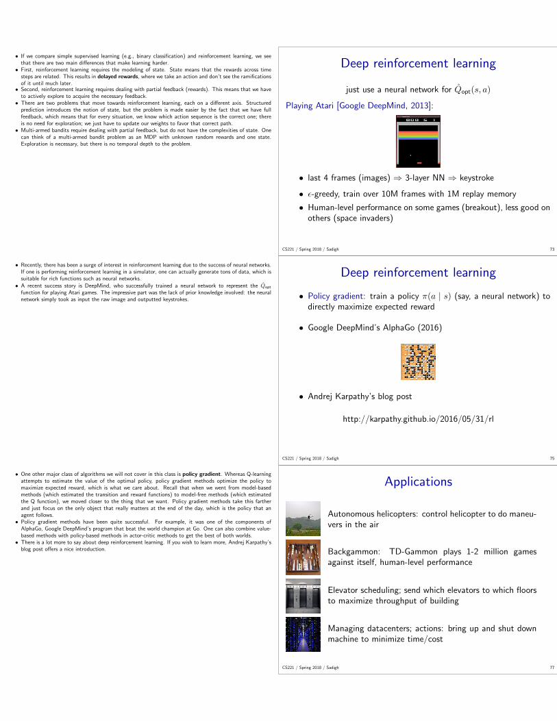
Deep reinforcement learning

just use a neural network for Q̂opt(s, a)

Playing Atari [Google DeepMind, 2013]:

• last 4 frames (images) ⇒ 3-layer NN ⇒ keystroke

• ε-greedy, train over 10M frames with 1M replay memory

• Human-level performance on some games (breakout), less good onothers (space invaders)


• Recently, there has been a surge of interest in reinforcement learning due to the success of neural networks.If one is performing reinforcement learning in a simulator, one can actually generate tons of data, which issuitable for rich functions such as neural networks.

• A recent success story is DeepMind, who successfully trained a neural network to represent the Q̂opt

function for playing Atari games. The impressive part was the lack of prior knowledge involved: the neuralnetwork simply took as input the raw image and outputted keystrokes.

Deep reinforcement learning

• Policy gradient: train a policy π(a | s) (say, a neural network) todirectly maximize expected reward

• Google DeepMind’s AlphaGo (2016)

• Andrej Karpathy’s blog post

http://karpathy.github.io/2016/05/31/rl


• One other major class of algorithms we will not cover in this class is policy gradient. Whereas Q-learningattempts to estimate the value of the optimal policy, policy gradient methods optimize the policy tomaximize expected reward, which is what we care about. Recall that when we went from model-basedmethods (which estimated the transition and reward functions) to model-free methods (which estimatedthe Q function), we moved closer to the thing that we want. Policy gradient methods take this fartherand just focus on the only object that really matters at the end of the day, which is the policy that anagent follows.

• Policy gradient methods have been quite successful. For example, it was one of the components ofAlphaGo, Google DeepMind’s program that beat the world champion at Go. One can also combine value-based methods with policy-based methods in actor-critic methods to get the best of both worlds.

• There is a lot more to say about deep reinforcement learning. If you wish to learn more, Andrej Karpathy’sblog post offers a nice introduction.

Applications

Autonomous helicopters: control helicopter to do maneu-vers in the air

Backgammon: TD-Gammon plays 1-2 million gamesagainst itself, human-level performance

Elevator scheduling; send which elevators to which floorsto maximize throughput of building

Managing datacenters; actions: bring up and shut downmachine to minimize time/cost


• There are many other applications of RL, which range from robotics to game playing to other infrastructuraltasks. One could say that RL is so general that anything can be cast as an RL problem.

• For a while, RL only worked for small toy problems or settings where there were a lot of prior knowledge/ constraints. Deep RL — the use of powerful neural networks with increased compute — has vastlyexpanded the realm of problems which are solvable by RL.

Markov decision processes: against nature (e.g., Blackjack)

Next time...

Adversarial games: against opponent (e.g., chess)


Documents

Q-value Q a bus 1 ride bus 17 ride the magic tram cs221.stanford.edu/q CS221 / Autumn 2017 / Liang & Ermon 1 In in the previous lecture, you probably had some model of the world (how