Embed Size (px)
Citation preview

© Qi Li 2011
All Rights Reserved

FAST PARALLEL MACHINE LEARNING ALGORITHMS FOR LARGE
DATASETS USING GRAPHIC PROCESSING UNIT
A Dissertation submitted in partial fulfillment of the requirements for the degree of Doctor of Philosophy at Virginia Commonwealth University.
by
QI LI M.S., Virginia Commonwealth University, 2008
B.S., Beijing University of Posts and Telecommunications (P.R. China), 2007
Director: VOJISLAV KECMAN ASSOCIATE PROFESSOR, DEPARTMENT OF COMPUTER SCIENCE
Virginia Commonwealth University Richmond, Virginia
December, 2011

ii
Table of Contents
List of Tables vi
List of Figures viii
Abstract ii
1 Introduction 1
2 Background, Related Work and Contributions 4
2.1 The History of Sequential SVM . . . . . . . . . . . . . . . . . . . . . 5
2.2 The Development of Parallel SVM . . . . . . . . . . . . . . . . . . . . 6
2.3 K-Nearest Neighbors Search and Local Model Based Classifiers . . . . 7
2.4 Parallel Computing Framework . . . . . . . . . . . . . . . . . . . . . 8
2.5 Contributions of This Dissertation . . . . . . . . . . . . . . . . . . . . 10
3 Graphic Processing Units 12
3.1 Computing Unified Device Architecture (CUDA) . . . . . . . . . . . 14
3.2 CUDA Programming Model . . . . . . . . . . . . . . . . . . . . . . . 14
3.3 CUDA Optimization Strategy . . . . . . . . . . . . . . . . . . . . . . 16
4 Similarity Search on Large Datasets 22
4.1 Distance Definition . . . . . . . . . . . . . . . . . . . . . . . . . . . . 24

iii
4.1.1 Weighted Euclidean Distance . . . . . . . . . . . . . . . . . . 24
4.1.2 Cosine Similarity . . . . . . . . . . . . . . . . . . . . . . . . . 25
4.1.3 Weighted Manhattan Distance . . . . . . . . . . . . . . . . . . 26
4.2 Distance Calculation Algorithms . . . . . . . . . . . . . . . . . . . . . 26
4.2.1 Classic Sequential Method . . . . . . . . . . . . . . . . . . . . 26
4.2.2 Parallel Method Using CUDA . . . . . . . . . . . . . . . . . . 30
4.3 Performance Results of Distance Kernel Function . . . . . . . . . . . 31
4.4 Data Partitioning and Distributed Computation . . . . . . . . . . . . 33
4.5 Parallel Sorting Using CUDA . . . . . . . . . . . . . . . . . . . . . . 36
4.5.1 Sequential Sort . . . . . . . . . . . . . . . . . . . . . . . . . . 37
4.5.2 Parallel Sort . . . . . . . . . . . . . . . . . . . . . . . . . . . . 42
4.5.3 Shell Sort . . . . . . . . . . . . . . . . . . . . . . . . . . . . . 44
4.5.4 Speed Comparison Test of Sorting Algorithms . . . . . . . . . 44
4.6 K-Nearest Neighbors Search using GPU . . . . . . . . . . . . . . . . . 45
5 Parallel Support Vector Machine Implementation Using GPUs 48
5.1 Two-Class SVM . . . . . . . . . . . . . . . . . . . . . . . . . . . . . . 49
5.1.1 Hard-Margin SVM . . . . . . . . . . . . . . . . . . . . . . . . 49
5.1.2 L1 Soft-Margin SVM . . . . . . . . . . . . . . . . . . . . . . . 53
5.1.3 Nonlinear SVM . . . . . . . . . . . . . . . . . . . . . . . . . . 55
5.2 Multiclass SVM . . . . . . . . . . . . . . . . . . . . . . . . . . . . . . 56
5.2.1 One-Versus-All . . . . . . . . . . . . . . . . . . . . . . . . . . 56
5.2.2 One-Versus-One . . . . . . . . . . . . . . . . . . . . . . . . . . 57
5.2.3 Comparison between OVA and OVO . . . . . . . . . . . . . . 58
5.3 N-Fold Cross Validation . . . . . . . . . . . . . . . . . . . . . . . . . 58
5.4 Platt’s SMO . . . . . . . . . . . . . . . . . . . . . . . . . . . . . . . . 59
5.5 Keerthi’s SMO . . . . . . . . . . . . . . . . . . . . . . . . . . . . . . 64
iv
5.6 Parallel SMO Using Clusters . . . . . . . . . . . . . . . . . . . . . . . 66
5.7 Parallel SMO Using GPU . . . . . . . . . . . . . . . . . . . . . . . . 67
5.7.1 Kernel Computation . . . . . . . . . . . . . . . . . . . . . . . 67
5.7.2 Cache Design . . . . . . . . . . . . . . . . . . . . . . . . . . . 68
5.7.3 GPU Acceleration . . . . . . . . . . . . . . . . . . . . . . . . . 71
6 A Glance of GPUSVM 77
6.1 GPUSVM Overview . . . . . . . . . . . . . . . . . . . . . . . . . . . 77
6.2 GPUSVM Implementation . . . . . . . . . . . . . . . . . . . . . . . . 78
7 GPUSVM Accuracy and Speed Performance Comparisons with
LIBSVM on Real-World Datasets 81
7.1 Host and Device . . . . . . . . . . . . . . . . . . . . . . . . . . . . . . 81
7.2 The Experimental Datasets . . . . . . . . . . . . . . . . . . . . . . . 82
7.3 The Accuracy Comparison Test on Small and Medium Datasets . . . 83
7.4 The Speed Performance Comparison Test on Small and Medium Datasets 85
7.5 Experimental Results for Different Epsilon on Medium Datasets . . . 88
7.6 Experimental Results on Large Datasets . . . . . . . . . . . . . . . . 89
7.7 The CV Performance Comparison Using Single GPU . . . . . . . . . 93
8 Conclusions and Future Work 96
List of References 99
Vita 105

v
List of Tables
4.1 Performance comparison of symmetric Euclidean distance matrix cal-
culation. . . . . . . . . . . . . . . . . . . . . . . . . . . . . . . . . . . 32
4.2 Performance comparison of asymmetric Euclidean distance matrix cal-
culation. . . . . . . . . . . . . . . . . . . . . . . . . . . . . . . . . . . 33
4.3 Performance result of chunking method on real-world large datasets. . 37
4.4 K-NNS performance comparison on MNIST (60,000 data points, 576
features). . . . . . . . . . . . . . . . . . . . . . . . . . . . . . . . . . 47
5.1 List of popular kernel functions. . . . . . . . . . . . . . . . . . . . . . 55
7.1 The experimental datasets and their hyperparameters for the Gaussian
RBF kernel. . . . . . . . . . . . . . . . . . . . . . . . . . . . . . . . . 83
7.2 The accuracy performance comparison between GPUSVM and LIB-
SVM on small and medium datasets. . . . . . . . . . . . . . . . . . . 84
7.3 The speed performance comparison between GPUSVM and LIBSVM
on small datasets. . . . . . . . . . . . . . . . . . . . . . . . . . . . . . 86
7.4 The speed performance comparison between GPUSVM and LIBSVM
on medium datasets. . . . . . . . . . . . . . . . . . . . . . . . . . . . 87
7.5 The accuracy performance comparison between CPU and GPU on large
datasets. . . . . . . . . . . . . . . . . . . . . . . . . . . . . . . . . . . 91

vi
7.6 The speed performance comparison between CPU and GPU on large
datasets. . . . . . . . . . . . . . . . . . . . . . . . . . . . . . . . . . . 92
7.7 The speed performance comparison among GPUSVM-S, GPUSVM-P
and LIBSVM. . . . . . . . . . . . . . . . . . . . . . . . . . . . . . . . 94

vii
List of Figures
3.1 The architecture of a typical CUDA-capable GPU. . . . . . . . . . . 13
3.2 CUDA device memory model. . . . . . . . . . . . . . . . . . . . . . . 15
3.3 CUDA thread organization. . . . . . . . . . . . . . . . . . . . . . . . 17
3.4 One level loop unroll in the kernel functions. . . . . . . . . . . . . . . 18
3.5 Non-coalesced reduction pattern and preferred coalesced reduction pat-
tern. . . . . . . . . . . . . . . . . . . . . . . . . . . . . . . . . . . . . 20
3.6 Different grid configurations for solving the vector summation problem
among four vectors. . . . . . . . . . . . . . . . . . . . . . . . . . . . . 21
4.1 The complete distance matrix and its partial distance matrices. . . . 23
4.2 Impact of different weights on classification. . . . . . . . . . . . . . . 25
4.3 CUDA blocks mapping for generalized distance matrix calculation. . . 31
4.4 Mapping between data chunks to the related distance submatrices. . . 34
4.5 Map-Reduce pattern for large distance matrix calculation. . . . . . . 35
4.6 Speed performance comparison of sorting algorithms for fixed k and
various matrix dimension. . . . . . . . . . . . . . . . . . . . . . . . . 46
4.7 Speed performance comparison of sorting algorithms for various k and
fixed matrix dimension. . . . . . . . . . . . . . . . . . . . . . . . . . . 47
5.1 A graphic representation of linear SVM. . . . . . . . . . . . . . . . . 50
5.2 One-Versus-All SVM classification. . . . . . . . . . . . . . . . . . . . 57

viii
5.3 One-Versus-All SVM classification using Winner-Takes-All strategy. . 58
5.4 A graphic representation when both Lagrangian multipliers fulfill the
constraints. . . . . . . . . . . . . . . . . . . . . . . . . . . . . . . . . 60
5.5 The design structure for cache. . . . . . . . . . . . . . . . . . . . . . 69
5.6 5-fold cross-validation steps for Gaussian kernels. . . . . . . . . . . . 74
5.7 Binary linear SVM training on the same dataset with four different C. 75
5.8 Same support vectors shared among the four tasks in Figure 5.7. . . . 75
6.1 GPUSVM: cross-validation interface. . . . . . . . . . . . . . . . . . . 78
6.2 GPUSVM: training interface. . . . . . . . . . . . . . . . . . . . . . . 79
6.3 GPUSVM: predicting interface. . . . . . . . . . . . . . . . . . . . . . 79
7.1 The accuracy performance for different ε values on medium datasets. 89
7.2 The number of support vectors for different ε values on medium datasets. 90
7.3 The speed performance for different ε values on medium datasets. . . 91
7.4 Training time comparison between GPUSVM and LIBSVM on large
datasets. . . . . . . . . . . . . . . . . . . . . . . . . . . . . . . . . . . 92
7.5 Predicting time comparison between GPUSVM and LIBSVM on large
datasets. . . . . . . . . . . . . . . . . . . . . . . . . . . . . . . . . . . 93
7.6 Independent task comparison on speed performance and number of
support vectors between GPUSVM and LIBSVM. . . . . . . . . . . . 95
7.7 Total number of kernel computations for GPUSVM-S and GPUSVM-P. 95

Abstract
This dissertation deals with developing parallel processing algorithms for Graphic Pro-
cessing Unit (GPU) in order to solve machine learning problems for large datasets.
In particular, it contributes to the development of fast GPU based algorithms for
calculating distance (i.e. similarity, affinity, closeness) matrix. It also presents the
algorithm and implementation of a fast parallel Support Vector Machine (SVM) us-
ing GPU. These application tools are developed using Computing Unified Device
Architecture (CUDA), which is a popular software framework for General Purpose
Computing using GPU (GPGPU).
Distance calculation is the core part of all machine learning algorithms because
the closer the query is to some data samples (i.e. observations, records, entries), the
more likely the query belongs to the class of those samples. K-Nearest Neighbors
(k-NNs) search is a popular and powerful distance based tool for solving classification
problem. It is the prerequisite for training local model based classifiers. Fast distance
calculation can significantly improve the speed performance of these classifiers and
GPUs can be very handy for their accelerations. Meanwhile, several GPU based
sorting algorithms are also included to sort the distance matrix and seek for the k-
nearest neighbors. The speed performances of the sorting algorithms vary depending
upon the input sequences. The GPUKNN proposed in this dissertation utilizes the
GPU based distance computation algorithm and automatically picks up the most
suitable sorting algorithm according to the characteristics of the input datasets.
Every machine learning tool has its own pros and cons. The advantage of SVM is
the high classification accuracy. This makes SVM possibly one of the best classifiers.
However, as in many other machine learning algorithms, SVM’s training phase slows

iii
down when the size of the input dataset increases. The GPU version of parallel SVM
based on parallel Sequential Minimal Optimization (SMO) implemented in this dis-
sertation is proposed to reduce the time cost in both training and predicting phases.
This implementation of GPUSVM is original. It utilizes many parallel processing
techniques to accelerate and minimize the computations of kernel evaluation, which
are considered as the most time consuming operations in SVM. Although the many-
core architecture of GPU performs the best in data level parallelism, multi-task (aka.
task level parallelism) processing is also integrated into the application to improve the
speed performance of tasks such as multiclass classification and cross-validation. Fur-
thermore, the procedure of finding worst violators are distributed to multiple blocks
on the CUDA model. This reduces the time cost for each iteration of SMO during the
training phase. All of these violators are shared among different tasks in multiclass
classification and cross-validation to reduce the duplicate kernel computations. The
speed performance results have shown that the achieved speedup of both the training
phase and predicting phase are ranging from one order of magnitude to three orders
of magnitude times faster compared to the state of the art LIBSVM software on some
well known benchmarking datasets.

Chapter 1
Introduction
Machine learning is a discipline targeted on designing and developing algorithms
which allow computers to learn based on empirical data and capture the characteris-
tics of interest in order to make a prediction for a new data query. All the collected
data can be considered as examples (training samples) which illustrate the relations
among the observed variables. Many important patterns can be recognized after ap-
plying the learning procedure. Supervised learning is one type of machine learning
techniques inferring a function using supervised data, which does the classification
or regression jobs. Classifiers are generated in the classification problems in which
both input feature vector �x and the related output label y are known. They are used
for classifying new data queries and give discrete output. On the other hand, if the
continuous output is required, a regression function will be created instead of a clas-
sifier. This dissertation mainly focuses on classification problems. Currently, there
are many well developed classification tools, e.g. Support Vector Machine, Neural
Network, Decision Tree, k-NNs search, etc. They all have certain advantages and
disadvantages in different scenarios. However, one of the common drawback among
them is the lack of scalability, which largely restricted their popularity and usage in
processing large datasets. The fact is that it is an era of exploded information now,
1

2
and large scale datasets are found everywhere. For instance, a mid-size social network
website can easily collect Tera-bytes of multimedia data such as users’ status change,
newly uploaded photos, daily notes, conversations and so on. Most of these raw data
are left unprocessed and archived due to the software limitations. However, these
data can be very useful to help learn the users’ preferences, interests and patterns of
their activities. The outcome is obvious. Better user experience always leads to more
customers. Therefore, the newly improved many-core GPUs are involved to help re-
duce the processing time for training large datasets. They are superbly fast in floating
points operations and small in physical size. The hardware cost is also much less and
so is the power consumption compared to CPUs which offer the same level of pro-
cessing capability. With the assists of GPUs, a proper equipped workstation can do
just about the same job which could only be done on a small clustering system in the
past. GPU’s popularity on solving data intensive applications is growing everyday.
In this dissertation, GPUs are used for developing fast parallel SVM software.
This dissertation is mainly focusing on developing and implementing classifica-
tion, a.k.a. pattern recognition, algorithms for GPUs. The NVIDIA Tesla GPUs
and CUDA software development kit are used as the main hardware and software
components for the sake of software implementation. However, the proposed paral-
lel processing algorithms, methodologies and optimization strategies are all original
and general, which can be extended and adapted to other platforms or frameworks.
They are all considered as the contributions of this dissertation. The final developed
GUI enabled SVM tool which has been configured and installed in the department’s
ACE-Tesla computer is also part of the contribution of this dissertation.
The original research objective includes the classic linear and non-linear SVM
design as well as the local model based classifiers such as Local Linear SVM [1] and
Adaptive Local Hyperplane [2]. The SVM part has been successfully finished in this

3
dissertation work. The crucial problem of the local model based classifiers, which is
the distance computation, has also been addressed in the dissertation. In Chapter
2, some existing work done on both sequential and parallel SVM implementation
are briefly reviewed. Major contributions of this dissertation are also listed in this
chapter. Chapter 3 discusses the detail information about GPU and NVIDIA’s CUDA
technology. CUDA programming model and optimization strategies are presented and
explained to help understand the proposed implementations in the later chapters.
Similarity search and distance computation is discussed in Chapter 4, which is the
fundamental of building local model based classifiers. The speed performance of the
proposed GPUKNN algorithm is also given. Chapter 5 reviews various decomposition
approaches such as Platt’s SMO, Keerthi et al.’s improved SMO and Cao et al.’s
parallel SMO in solving Quadratic Programming (QP) problem, which is the core of
SVM solver. This chapter also introduces the proposed GPUSVM algorithm. Chapter
6 describes the hierarchy design architecture of the GPUSVM package. Chapter
7 presents the simulations and comparisons between the state of the art LIBSVM
software and the GPUSVM software. The comparisons are done for both accuracy
and speed performances on several benchmarking datasets of various sizes. The results
have shown the impressive speed performance of the novel GPUSVM over LIBSVM
while achieving very close accuracies. Chapter 8 gives the conclusions and points out
some possible future work as the continuation of this dissertation.

Chapter 2
Background, Related Work and
Contributions
This chapter first briefly reviews the historical development of sequential SVM al-
gorithms and parallel SVM algorithm. Parallel SVM algorithm used to be not very
popular a decade ago compared to its sequential counterpart. There is much less re-
search done on parallel SVM due to the lack of the availability for parallel hardware.
However, it becomes more and more popular recently not only because sequential
SVM suffers from a very slow training phase on large datasets, but also due to the
huge improvement and the availability of the cheap and easy to program parallel
hardware. K-NNs search is another classic classification tool, which recently has also
been used for building local model based classifiers. These classifiers have good ac-
curacy and they can be trained efficiently in parallel. Some of these classifiers are
reviewed in this chapter. The core of k-NNs search is distance calculation which
has been addressed in this dissertation using powerful GPUs. Then several exist-
ing mature parallel processing framework are discussed and compared to show their
advantages and disadvantages. They are good options for creating parallel machine
learning tools. At the end, the contributions of this dissertation are given.
4

5
2.1 The History of Sequential SVM
Support Vector Machine [3, 4] is a learning algorithm which has become popular
due to its high accuracy performance. It solves both the classification and regression
problems. Nevertheless, the training phase of an SVM could be a computationally
expensive task especially for large datasets, because the core of the training is solving
a QP problem. Solving large QP problem with numeric method can be very compli-
cated, time consuming and memory inefficient. More details of solving QP problem
are explained in Chapter 5. There are countless efforts and research which have been
put on how to reduce the training time of SVM. After Vapnik invented SVM, he
proposed a method known as “chunking” to break down the large QP problem into a
series of smaller QP problems. This method seriously reduces the size of the matrix
but it still cannot solve large problem due to the computer memory limitations at
that time. Osuna et al. presented a decomposition approach using iterative meth-
ods in [5]. Joachims introduced practical techniques such as shrinking and kernel
caching in [6], which are common implementation in many modern SVM software.
He also published his own SVM software called SVMLight [6] using these techniques.
Platt invented SMO [7] to solve the standard QP problem by iteratively solving a QP
problem with only two unknowns using analytic methods. This method requires very
small amount of computer memory. Therefore it addresses the memory limitation
issue brought by large training datasets. Kecman et al. [4] proposed the Iterative
Single Data Algorithm (ISDA) which uses a single sample during every iteration of
the optimization, which performs a coordinate descent search for a minimum of the
cost function. ISDA has shown to have all the good properties of SMO algorithm
while being slightly faster. Later on, Keerthi et al. developed an improved SMO in
[8] which resolves the slow convergence issue in Platt’s method. More recently, Fan et
al. introduced a series of working set selection [9], which further improves the speed

6
of convergence. These methods have been implemented and integrated in the state of
the art LIBSVM software [10]. These major work summarize the background details
of how to implement a fast classic SVM in sequential programming.
2.2 The Development of Parallel SVM
Compared to the sequential SVM, there is not much of research done on parallel SVM.
However, the development of fast parallel SVM is still a very hot research topic. Some
earlier works using parallel techniques in SVM can be found in [11], [12], [13] and
[14]. Cao et al. presented a very practical Parallel Sequential Minimal Optimization
(PSMO) [15] implemented with Message Passing Interface on a clustering system.
The performance gain of training SVM using clusters shows the beauty of parallel
processing. This method is also the foundation of the proposed GPUSVM here. Graf
et al. introduced the Cascade SVM [16] which decomposes the training dataset to
multiple chunks and trains them separately. Then the support vectors from different
individual classifiers are combined and fed back to the system again. They proved that
the global optimal solution can be achieved by using this method. This method uses
task level parallelism compared to the data level parallelism in Cao et al.’s method.
Cascade SVM offers a new way to handle ultra-large datasets training. Catanzaro et
al. proposed a method to train a binary SVM classifier using GPU in [17]. Significant
speed improvements were reported compared to the LIBSVM software. The latest
GPU version of SVM was from Herrero-Lopez et al. [18]. They enabled the possibility
to solve multiclass classification problems using GPU.

7
2.3 K-Nearest Neighbors Search and Local Model
Based Classifiers
Although classic SVM shows its elegance in many aspects, researchers also put lots
of efforts on other different variants of SVM. Some of them such as Iterative Single
Data Algorithm mentioned earlier uses a single sample in solving QP problem. Others
use approximate models such as Proximal SVM [19, 20]. Kecman et al. explore
the possibility of combining local linear SVMs to approximate the global optimal
solution in [1]. Similar work is also shown in [21, 22]. This local model idea starts an
innovative trend with combination of various other classifiers. The Adaptive Local
Hyperplane [2] is one of the best. Yang and Kecman’s results have shown that ALH
beats most of other classifiers on classification accuracy for several popular datasets.
However, finding the optimal local model requires performing k-NNs search on the
training dataset. This can be very time consuming since the training stage must test
through a series of different k values. One of the typical way of finding k-NNs is using
Tree structure [23]. However, this type of method has limited speed performance in
the cases when training datasets have large feature space. Besides, doing repeated
individual k-NNs search is not very practical for training local model based classifiers
in terms of speed performance. The better approach would be computing the distance
matrix of the training dataset in advance and then sort it with indexes by either rows
or columns. Thus k-NNs can be easily located in the index matrix with whatever
given k value without performing the search operation. The disadvantage of this
method is the high cost of the distance matrix computation. This disadvantage can
be offset by utilizing the computational power of GPUs. The earliest implementation
of GPU based Euclidean distance calculation is introduced by Chang et al. in [24],
but their proposed implementation is too simple to be useful in application design.

8
A more practical implementation can be found in [25]. The complete GPU KNN
algorithm was first implemented by Garcia et al. [26]. However, they use a modified
insertion sort which only sorts a portion of the distance matrix. Thus it involves
duplicated distances computation when a series of k values are tested. Furthermore,
there are neither options for using other metrics nor for an inclusion of the weights in
the distance computation. Weighted Euclidean distance computation is a necessary
part of ALH algorithm. Our research is an extension of [25, 27] which includes the
weighted Euclidean distance, cosine similarity and Manhattan distance calculation
using GPUs. It will be integrated into the Local Linear SVM and ALH to improve
their speed performance during the training phase in the future.
2.4 Parallel Computing Framework
There are many existing parallel programming tools and models proposed for differ-
ent architecture of computer systems in the past decade. Message Passing Interface
(MPI) [28] and OpenMP [29] are two of the most widely used parallel models which
are designed for main stream computing systems. MPI is a model in which computing
nodes do not share memory with each other. It is commonly used in a distributed
environment such as a clustering system. All data sharing and exchange must be
done through explicit message communications. A typical setup of MPI model in-
cludes a master node and a group of slave nodes. The master node scatters the data
to the slave nodes and gathers the results back after the computations have finished
on the slave nodes. Most of the synchronizations are done on the master node. Per-
formance of MPI system is highly related to the speed of intra-network connection
due to the large amount of data exchange. Thus many MPI based algorithms are
optimized to minimize these data exchange. The lack of the shared memory access
across multiple computing nodes requires a significant amount of work on the appli-

9
cation design. OpenMP supports shared memory, which is more commonly used in
the standard workstation systems and multi-core personal computers. Shared mem-
ory system usually has a smaller scale compared to the distributed system. The
scalability of OpenMP are restricted compared to MPI. Furthermore, the require-
ment of precise threads management will not allow the OpenMP to generates many
threads due to the cost of threads overhead, threads context switching and threads
synchronization. Besides, if the amount of threads exceeds the number of computing
cores, time-division multiplexing is used by computing cores to switch between phys-
ical threads. Therefore it is less likely to improve the performance by creating more
threads, which just involves extra computations. The advantage of OpenMP is the
boost on the performance of existing applications by using multi-core system with
minimal amount of modifications on the original algorithms if they are applicable.
For example, algorithms running data independent tasks in a large loop structures
can be easily accelerated with OpenMP.
GPU’s programming model is kind of a mixture of both message passing and
shared memory with some of its own unique features. First of all, there is no shared
memory access between GPUs and CPUs. All the data must be transferred from
the main memory to the device memory for processing, which behaves the same
as MPI model does. Secondly, there are shared memory which can be accessed
by all threads within a block but threads from different blocks inside of the GPU.
This shows certain similarity feature to shared memory model. Furthermore, GPU
threads are lightweight and efficient. They are much simpler in structure compared
to CPU threads with less overhead, which makes it possible to generate huge amount
of threads for massive parallel processing. More details about GPU programming
model will be introduced in Section 3.2. More recently, several major industry players
including Apple, Intel, AMD/ATI and NVIDIA have jointly developed a standard-

10
ized programming model called Open Computing Language (OpenCL) [30]. OpenCL
shares many common aspects from CUDA but it is still not very mature which makes
it less popular on NVIDIA GPUs. Therefore CUDA is used for implementing the
proposed algorithm in order to achieve the maximum speed gain by using the latest
hardware from NVIDIA.
2.5 Contributions of This Dissertation
Although there is plenty of research done using GPU to improve speed performance
of complex algorithms, many applications are still theory oriented and lack practical
usage. This dissertation not only introduces the parallel SVM algorithm and distance
calculation algorithms designed for GPU programming, but it also implements them
using CUDA framework and makes them practical for processing real-world datasets.
As it has been mentioned in the previous section, the author develops the algorithms
in a way that they can be ported to other platform such as OpenCL. The GPUKNN
search algorithm introduced in this dissertation, which is the fundamental for the
use of local model based classifiers, combines the fast distance calculation and sorting
using GPU. By largely reducing the time cost of k-NNs search, the speed performance
of LLSVM and ALH is expected to be improved heavily. Furthermore, not only does
this practical application offer the choice for different distance metrics, but it is also
smart to pick up the proper sorting algorithm for the best performance depending
upon the characteristics of input datasets.
The CUDA implementation of parallel SVM developed in this dissertation has
achieved great performance using Fermi series Tesla GPUs, which are the second
generation hardware platform for CUDA. The software utilizes the parallelism in
both data level and task level to maximize the performance of one single GPU card
or several GPU cards operating simultaneously. It also leverages the computation

11
load between CPU and GPU. This helps improving the efficiency of the GPUSVM
algorithm. The current implementation of the GPUSVM outperforms the state of
the art LIBSVM tool in speed performance for both training phase and predicting
phase. It also has as good accuracy performance as LIBSVM. Besides, the software is
compatible with previous generation of GPUs and it is practical in solving real-world
problems. It supports multi-GPU system to enable even further speed improvement
on cross-validation training, which is a slow procedure on classic sequential machines.
The software is developed using a three-layer structure. The bottom layer written in
CUDA has an SVM solver and a predictor for SVM training and predicting functions.
The middle layer written in Python offers command line interface to call the solver
and predictor. It also contains utility functions of scaling the data files, shuffling
the input datasets, running cross-validations and some other tasks related to SVM.
The upper layer written in JAVA offers a user friendly graphic user interface for easy
operation.

Chapter 3
Graphic Processing Units
GPUs are micro processors commonly seen on video cards. The main function of GPU
is offloading and accelerating the graphic rendering jobs from the CPU. Rendering is
a process of generating an image from a model by a set of computer programs and
it usually involves floating point intensive computations based on various mathemat-
ical equations. Thus, before 2006, most of these GPUs were designed in a way that
computing resources were partitioned into vertexes and pixel shaders. Even though
the hardware of GPUs have matured for intensive floating point computations, there
is no other way but using OpenGL or DirectX to access the features in GPUs. Smart
programmers disguised their general computations to graphic problems in order to
utilize the hardware capability of GPU. They were the first who started to use GPUs
to solve general purpose computing problems. In order to overcome this inflexibility,
NVIDIA introduced the GeForce 8800 GTX in 2006, which maps the separated pro-
grammable graphics stages to an array of unified processors. Figure 3.1 shows the
shader pipeline of GeForce 8800 GTX GPU. It is organized into an array of highly
threaded streaming processors (SMs). In Figure 3.1, two SMs form a building block;
however, the number of SMs in a building block can vary between different genera-
tions of CUDA GPUs. Each SM in Figure 3.1 has a number of streaming processors
12

13
(SPs) that share control logic and instruction cache. Each GPU currently comes with
up to 6GB (e.g. Tesla C2070) GDDR DRAM, referred to as global memory. These
global memory are essentially the frame buffer memory that is used for graphics. For
graphics applications, they hold video images and texture information for render-
ing, but for computing purpose they function as high bandwidth off-chip memory.
All later GPU products from NVIDIA follow this design philosophy thus they are
capable of general purpose computing and referred to as CUDA capable devices.
Figure 3.1: The architecture of a typical CUDA-capable GPU.
The latest Tesla GPU has the shader processors (cores) fully programmable with
large instruction memory, instruction cache and instruction sequencing control logic.
In order to reduce the total hardware cost, several shader processors will share the
same instruction cache and instruction sequencing control logic. The Tesla architec-
ture introduced a more generic parallel programming model with a hierarchy of par-
allel threads, barrier synchronization and atomic operations to dispatch and manage
highly parallel computing work. Combined with C/C++ compiler, libraries, runtime

14
software and other useful components, CUDA Software Development Kit is offered
to developers who do not posses the programming knowledge of graphic applications.
With a minimal learning curve of some extended C/C++ syntax and some basic
parallel computing techniques, developers can start migrating existing projects using
CUDA with NVIDIA GPUs. Introductions of CUDA programming model and its
related optimization strategies are given in the following sections.
3.1 Computing Unified Device Architecture
(CUDA)
CUDA is a software platform developed by NVIDIA to support their general purpose
computing GPUs for easy programming and porting existing applications to GPUs.
It primarily uses C/C++ syntax and a few new keywords as an extension, which offers
a very low learning curve for an application designer. The latest CUDA version has
been supported by various third parties. Many toolboxes and plug-ins can be found
to help increase the productivity. CUDA memory model and thread organization is
introduced in this part.
3.2 CUDA Programming Model
Figure 3.2 shows the memory model of the CUDA device. The device codes can read-
/write per-thread registers; read/write per-block shared memory; read/write per-grid
global memory; read only per-grid constant memory. The host codes can transfer
data to/from per-grid global and constant memory. Constant memory offers faster
memory access to CUDA threads compared to global memory. The threads are or-
ganized in a hierarchical structure. The top level is a grid which contains blocks of
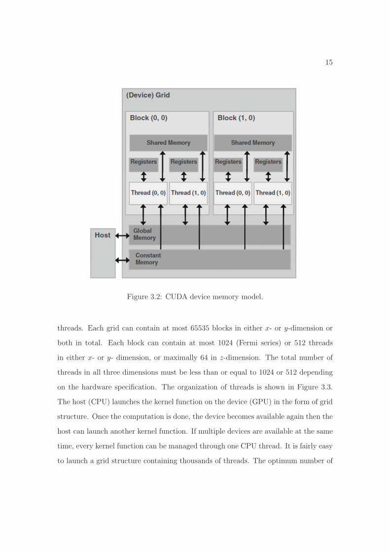
15
Figure 3.2: CUDA device memory model.
threads. Each grid can contain at most 65535 blocks in either x- or y-dimension or
both in total. Each block can contain at most 1024 (Fermi series) or 512 threads
in either x- or y- dimension, or maximally 64 in z-dimension. The total number of
threads in all three dimensions must be less than or equal to 1024 or 512 depending
on the hardware specification. The organization of threads is shown in Figure 3.3.
The host (CPU) launches the kernel function on the device (GPU) in the form of grid
structure. Once the computation is done, the device becomes available again then the
host can launch another kernel function. If multiple devices are available at the same
time, every kernel function can be managed through one CPU thread. It is fairly easy
to launch a grid structure containing thousands of threads. The optimum number of

16
thread and block configuration varies among different applications. To achieve bet-
ter performance, there should be at least thousands or tens of thousands of threads
within one grid. It would not make much sense to use too few threads to extract
maximal performance from hardware. However, too many threads whose number
exceeds the number of data would also increase the thread overhead and bring down
the efficiency. The multiprocessor creates, manages, schedules, and executes threads
in groups of 32 parallel threads called warps. Thus a multiple of 32 could be a good
candidate value for the optimal number of threads per block. Threads within the
same block have limited shared memory and they are able to communicate with each
other by using these shared memory. All threads have their own registers and access
to the global memory as well as the constant memory. The size of the global memory
can be as large as up 6GB (depending on the GPU hardware). Similar to Message
Passing Interface (MPI), there is no shared memory between host and device thus the
data must be transferred from the host memory to device memory in the first place.
The result must also be transferred back for future processing or storage.
3.3 CUDA Optimization Strategy
Optimizations generally are targeted on improving certain algorithms with maximum
utilization of hardware. Several techniques which have been used in the proposed
algorithms are given here. The first one is loop unrolling which is shown in Figure
3.4. Loop unrolling has been used in sequential programming for a long time. Most
modern compilers automatically unroll the loop in certain degrees to achieve better
performance. In the simple example below, the loop structure is executed only once
in the unrolled version instead of twice in the normal version. The advantage is that
each thread can now process two data elements without using an extra loop. It is
true in most situations that not enough threads can be created to match the total

17
Figure 3.3: CUDA thread organization.
number of data. Thus, each thread may process more than one data element, which
requires the usage of loop structure. Think about how to write a code to do vector
summation in sequential way. It can be done like this:
int idx = 0;
while(idx < n) {
sum[idx] = a[idx] + b[idx];
++idx;

18
Figure 3.4: One level loop unroll in the kernel functions.
}
Similarly, writing a CUDA kernel function to do the same job looks like the following:
int idx = blockIdx.x * blockDim.x + threadIdx.x;
int shift = gridDim.x * blockDim.x;
while(idx < n) {
sum[idx] = a[idx] + b[idx];
idx += shift;
}

19
To reduce the overhead of loop, common practice suggests doing one level of loop
unrolling as shown below.
int idx = blockIdx.x * (blockDim.x * 2) + threadIdx.x;
int shift = gridDim.x * blockDim.x * 2;
while(idx < n) {
sum[idx] = a[idx] + b[idx];
if(idx + blockDim.x < n) {
sum[idx + blockDim.x] = a[idx + blockDim.x] + b[idx +
blockDim.x];
}
idx += shift;
}
CUDA compiler does not support automatic loop unrolling like sequential program-
ming compilers due to the complexity of condition checking mechanism. Thus it is
the developers’ job to write loop unrolling statements in the source code.
Another commonly used technique is reduction. Because threads from different
blocks cannot communicate with each other, the results returned from each block
compose a vector. In most applications, since the results are distributed to many
blocks for parallel processing, they require the summation of the distributed results
and this is so called reduction. Figure 3.5 shows both inefficient reduction pattern
and preferred reduction pattern. It is important to let the threads access the global
memory in a coalesced manner to achieve the best performance. The correct imple-
mentation of reduction technique is much more complex than what is shown in the
figure. Threads must be synchronized at every stage and reductions stop at the block
level since there are no threads communication among blocks. Thus, to compute the
final result the complete reduction will require multiple launches of kernel functions
with reduced grid size until the total number of blocks in the grid becomes one. Re-
duction can be utilized to implement MAX, MIN, SUM and some other functions

20
which are basic but very useful.
Figure 3.5: Non-coalesced reduction pattern and preferred coalesced reduction pat-tern.
The third commonly used technique is the utilization of shared memory. GPUs
are fast on floating points operations but not on memory accessing operations. If
a program requires frequently access to memories, it might not be able to achieve
better performance by using GPUs. Although GPU can have global memory as large
as 6GB, the amount of shared memory is very limited. Assuming a problem which
computes summations of any two vectors among four different vectors, there are six
different combinations as a group of two vectors. Thus creating six rows of blocks
to compute the results is most intuitive idea as our first response. However, this

21
configuration is shown as Grid 0 in Figure 3.6. Each vector must be read three times
from the global memory. Instead, Grid 1 configuration reduces the number of reads
for the same vectors to two, but every row block must compute two results. In order
to let the threads share data between two vector summations, shared memory must
be involved to store the data read from the global memory. In the configuration of
Grid 2, vector A is read only once but all other vectors are read twice. This does very
small improvement compared to Grid 1 in terms of memory accessing operations but
it requires much more shared memory, which might be not satisfied in some scenarios.
Thus, how to design the grid configuration and maximize the usage of limited shared
memory is an important concern for producing efficient codes. One good example
is the matrix multiplication which can be found in CUDA SDK sample codes. Our
fast distance computation routine in the next Chapter carries similar idea behind the
scene.
Figure 3.6: Different grid configurations for solving the vector summation problemamong four vectors.

Chapter 4
Similarity Search on Large
Datasets
Measuring similarity (i.e. distance, affinity, closeness) between different samples is the
fundamental approach in pattern recognition. This approach is based on the belief
that the closeness in a feature space means similarity between two samples. Similarity
search is based on the comparisons among distances. Euclidean, cosine and Manhat-
tan distances are common similarity metrics which are used in many machine learning
algorithms. The idea behind the similarity search is that a smaller distance between
two data points may indicate a stronger or closer relationship between them. General
distance matrix for a dataset is a symmetric square matrix containing distances from
each data point to all other data points including itself. When the total number
of samples grows large, it is usually not feasible to compute or store the complete
distance matrix in the system memory. For example, a dataset containing 100,000
samples could cost approximately 40GB space in single precision format and twice of
that in double precision. Obviously, half of them can be reduced due to the symmetric
property, however it is still not practical in real-world application design. Therefore
most of distance computations are done in real time or precalculated in advance. A
22

23
fragment of the complete distance matrix is referred to as a partial distance matrix
shown in Figure 4.1. It contains distances between one set of data points to another
set of data points, which could have different number of samples. Partial distance
matrix can be asymmetric and rectangular. It is used for reproducing the original
complete distance matrix.
Figure 4.1: The complete distance matrix and its partial distance matrices.
This chapter addresses the issue of how to utilize the power of GPU to accelerate
the time consuming distance matrix computation. The definitions of three major
distance kernels are given at the beginning and then the classic algorithms as well
as the parallel algorithm using CUDA for distance calculation are introduced. Data
partitioning and distributed computing techniques for large distance matrix are also
presented. And then a few parallel sorting algorithms are given to build the complete
GPU based GPUKNN software. This tool has a good speed performance in solving
k-NNs search problem compared to the classic sequential algorithm. The results of
the speed performance on calculating distance matrix, sorting and the GPUKNN are
given at the end of the chapter.

24
4.1 Distance Definition
Define two matrices A and B. A contains nA samples and each sample has m features.
Each row represents one data sample from the dataset. B has nB samples and it is
organized in the same format as A. The distance matrix DAB between A and B is an
nA by nB matrix where each row represents the distances between one data sample
from A to all data samples from B. The distance value dij represents the distance
between data sample �ai and data sample �bj.
4.1.1 Weighted Euclidean Distance
Weighted Euclidean distance is a more generalized Euclidean distance, also known
as weighted L2-norm distance, which offers the option of specifying a weight for each
different feature. It is defined by
dij =
√√√√m∑
k=1
wk(aik − bjk)2. (4.1)
When all weights are equal to one, weighted Euclidean Distance becomes to the stan-
dard Euclidean Distance. If wk = 0, the kth feature will be eliminated in distance
calculation. Weighted Euclidean distance becomes useful when the features have dif-
ferent impacts on the classification result. In Figure 4.2, the solid green line defines
the best separation boundary. Both features must be used for computing this separa-
tion line. However, the dashed yellow line can also separate the two classes without
any failure and it only uses feature 1. It is obvious that correct classification cannot
be done using just feature 2. This indicates that using a bigger weight for feature
1 compared to feature 2 might yield better classification result. If the weights are
proper chosen, weighted Euclidean distance performs better than standard Euclidean
distance. Many advanced machine learning models such as ALH in [2] use weighted

25
Figure 4.2: Impact of different weights on classification.
Euclidean distance.
4.1.2 Cosine Similarity
Cosine similarity, a.k.a. cosine distance is defined as
dij =�aT
i ·�bj
‖�ai‖‖�bj‖=
m∑k=1
aikbjk
√√√√m∑
k=1
a2ik
√√√√m∑
k=1
b2jk
. (4.2)
Cosine similarity is a useful measurement in documents comparison and text mining.
Weighted cosine similarity is not widely used.

26
4.1.3 Weighted Manhattan Distance
Weighted Manhattan distance is another popular distance measurement similar to
weighted Euclidean distance. It is also referred as weighted L1-norm distance, which
is defined as
dij =m∑
k=1
wk|aik − bjk| (4.3)
4.2 Distance Calculation Algorithms
4.2.1 Classic Sequential Method
Algorithm 1 shows the standard procedure of calculating distances between two
datasets. This method involves a nested for loop structure, which leads to a polyno-
mial time complexity of O(nAnBm) a.k.a. cubic time. Considering the size of feature
space is much smaller than the number of data samples, the time complexity is re-
duced to quadratic O(n2) in many cases. However, algorithms having quadratic time
complexity are still very slow and time consuming. A good property of Euclidean
distance is that the computations for the distance matrix can be broken down to
matrix level operations. In this way, the nested loop structure for pair-wise distance
computation can be removed. This is shown in Algorithm 2.
The idea of this algorithm is computing the weighted Euclidean distance matrix
using three partial distance matrices directly shown in Equation 4.4 instead of com-
puting every pair of distance one by one using loops.
DAB =√
P1 + P2 − 2P3. (4.4)
The square root operation on the matrix is doing element-wise square root. The three

27
Algorithm 1 Classic sequential distance calculation using loops.
1: load A, B, �w and allocate memory for DAB
2: for i = 1 to nA do3: for j = 1 to nB do4: dij = computeEucDist(�ai, �bj, �w)
5: or dij = computeCosDist(�ai, �bj)
6: or dij = computeManDist(�ai, �bj,�w)7: end for8: end for9: return DAB
10: computeEucDist(�ai, �bj, �w)11: d = 012: for k = 1 to m do13: d = d + wk(aik − bjk)
2
14: end for15: d =
√d
16: return d17:18: computeCosDist(�ai, �bj)19: p = pa = pb = 020: for k = 1 to m do21: p = p + aikbjk
22: pa = pa + aikaik
23: pb = pb + bjkbjk
24: end for25: d = p/(
√pa√
pb)26: return d27:28: computeManDist(�ai, �bj,�w)29: d = 030: for k = 1 to m do31: d = d + wk|aik − bjk|32: end for33: return d

28
Algorithm 2 Matrix operation based method for weighted Euclidean distance.
1: load A, B, �w and allocate memory for DAB
2: �v1 = (A · A)�w3: �v2 = (B · B)�w4: P1 = [�v1 �v1 . . . �v1]5: P2 = [�v2 �v2 . . . �v2]
T
6: W = [�w �w . . . �w]T
7: P3 = A(B · W)T
8: DAB =√
P1 + P2 − 2P3
9: return DAB
partial distances matrices are P1, P2 and P3 and they are expressed as
P1 =
⎡⎢⎢⎢⎢⎢⎢⎢⎣
m∑k=1
wka21k · · ·
m∑k=1
wka21k
.... . .
...m∑
k=1
wka2nAk · · ·
m∑k=1
wka2nAk
⎤⎥⎥⎥⎥⎥⎥⎥⎦
= [�v1 �v1 . . . �v1]. (4.5)
P2 =
⎡⎢⎢⎢⎢⎢⎢⎢⎣
m∑k=1
wkb21k · · ·
m∑k=1
wkb2nBk
.... . .
...m∑
k=1
wkb21k · · ·
m∑k=1
wkb2nBk
⎤⎥⎥⎥⎥⎥⎥⎥⎦
=
⎡⎢⎢⎢⎢⎢⎢⎢⎣
�vT2
�vT2
...
�vT2
⎤⎥⎥⎥⎥⎥⎥⎥⎦
. (4.6)
P3 =
⎡⎢⎢⎢⎢⎢⎢⎢⎣
m∑k=1
wka1kb1k · · ·m∑
k=1
wka1kbnBk
.... . .
...m∑
k=1
wkanAkb1k · · ·m∑
k=1
wkanAkbnBk
⎤⎥⎥⎥⎥⎥⎥⎥⎦
. (4.7)
Matrices P1 and P2 shown in Equation 4.5, 4.6 are composed by vector �v1 and vector
�v2. The weight vector �w is shown in
�w = [w1 w2 ... wk]T . (4.8)

29
Vector �v1 is acquired by
�v1 = [m∑
k=1
wka21k,
m∑k=1
wka22k, ...,
m∑k=1
wka2nAk]
T
= (A · A)�w (4.9)
and vector �v2 is acquired by
�v2 = [m∑
k=1
wkb21k,
m∑k=1
wkb22k, ...,
m∑k=1
wkb2nBk]
T
= (B · B)�w. (4.10)
The partial distance matrix P3 is computed by
P3 = A(B · W)T . (4.11)
When all weights are equal to 1, the weighted Euclidean distance becomes standard
Euclidean distance and Equation 4.11 changes to
P3 = ABT . (4.12)
The matrix multiplication in Equation 4.11 or 4.12 takes most of the computation
time in Euclidean distance calculation. The naive implementation yields exact same
quadratic time complexity. However, CUDA has its own fast Basic Linear Algebra
Subroutines called CUBLAS [31]. The weighted Euclidean distance calculation can be
accelerated by calling matrix-matrix multiplication routine from CUBLAS. This im-
plementation turns out to have improved time complexity compared to the quadratic
one. When it comes to the cosine similarity and weighted Manhattan distance, there
is no way to transform the distance matrix computations to simple matrix opera-

30
tions thus routines from CUBLAS are useless. Although, the time complexity stays
in quadratic, the time cost of distance computations can still be reduced by using
parallel techniques. A general GPU based parallel distance computation algorithm
is introduced in the following section. It can be used for all three metrics and it
offers as good speed performance as using CUBLAS for weighted Euclidean distance
computations as well.
4.2.2 Parallel Method Using CUDA
In order to map the distance calculation to the CUDA programming model, the GPU
kernel function utilizes a 2-D grid and uses shared memory to reduce the duplicated
memory fetching operations. The size of the block within the grid is set to 16 by 16.
The following code is used for initialization.
#define BLOCK_DIM 16
dim3 dimBlock(BLOCK_DIM ,BLOCK_DIM ,1);
dim3 dimGrid ((nA+BLOCK_DIM -1)/BLOCK_DIM ,
(nB+BLOCK_DIM -1)/BLOCK_DIM ,1);
In this way, the size of the grid will depend upon the input. It overcomes the imple-
mentation issue in [24] and supports input datasets with any dimensionality and any
number of data points. The pseudo code provided in [24] requires the input feature
space as a multiple of 32 and the input number of data points as a multiple of 2,
which are not practical in real-world applications. Figure 4.3 shows how the kernel
function works. Most blocks compute 256 pairwise distances. Some blocks located
on the bottom edge or the right edge of the grid may compute less than 256 pairwise
distances. That means some threads allocated in these blocks are not involved for the
computation. This cannot be avoid when the input datasets are irregular, which do
not have the number of data points as a multiple of 16. The shared memory is used
for storing the values of the features and the values of the weights. Feature values can

31
be reused in calculation of 16 pairwise distances and the weight values can be reused
in calculation of all 256 pairwise distances in that block. This significantly reduces
the time cost of global memory access.
Figure 4.3: CUDA blocks mapping for generalized distance matrix calculation.
4.3 Performance Results of Distance Kernel
Function
The following results are published in [25] generated by a workstation equipped with
the first generation of Tesla cards. The workstation has an Intel Xeon E5462 2.8GHz
quad-core CPU and 16GB RAM. There are three Tesla C1060 GPU devices connected
to the system through PCI Express interface. Each of these cards has 4GB device
memory. The CUDA 3.0 toolkit is used and the driver version is 195.36.15 for 64bit

32
Linux system. The operating system is Fedora Core 10 Linux. The benchmark of
GPU algorithms includes two ways of data transferring time between host memory
and device memory as well as the computational time on the GPU.
Table 4.1 shows the normal Euclidean distance matrix calculation comparison
among naive C implementation, MKL based C implementation, Chang et al.’s CUDA
implementation [24], and the proposed generalized CUDA implementation. It is easy
to observe that using MKL and multi-thread support for CPU can boost the perfor-
mance 5 to 6 times, thus comparison with the naive C implementation does not truly
reflect the performance gain by using GPU. Our implementation is slightly slower in
these special cases (both n and m are multiple of 16) compared to Chang et al.’s im-
plementation because the kernel function has been modified to suit general datasets,
which cannot be used by Chang et al.’s method. It takes two datasets as input,
thus the same dataset is copied twice from the system memory to the device mem-
ory in theses special cases. In general, the GPU implementation still has a speed-up
of approximately 5 times compared to MKL which is in the reasonable range based
on the performance comparison of matrix-matrix multiplication between MKL and
CUBLAS shown in [32].
Table 4.1: Performance comparison of symmetric Euclidean distance matrix calcula-tion.
Input matrix Naive Efficient Chang et al.’s Generalizedn C C (MKL) CUDA CUDA
4096 11.9 2.40 (4.96x) 0.36 (33.06x) 0.47 (25.32x)8192 48.4 8.49 (5.70x) 1.42 (34.08x) 1.79 (27.04x)12288 108.8 18.26 (5.96x) 3.16 (34.40x) 3.82 (28.48x)
Time unit is second and the size of feature space is 1024. Speed up is related to thenaive C implementation. Value n is number of data points.
Table 4.2 shows the performance comparison of calculating generalized distance
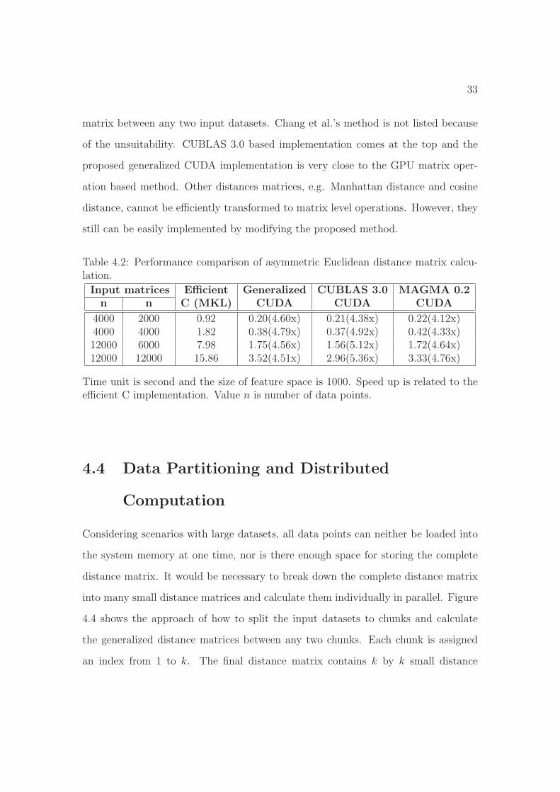
33
matrix between any two input datasets. Chang et al.’s method is not listed because
of the unsuitability. CUBLAS 3.0 based implementation comes at the top and the
proposed generalized CUDA implementation is very close to the GPU matrix oper-
ation based method. Other distances matrices, e.g. Manhattan distance and cosine
distance, cannot be efficiently transformed to matrix level operations. However, they
still can be easily implemented by modifying the proposed method.
Table 4.2: Performance comparison of asymmetric Euclidean distance matrix calcu-lation.
Input matrices Efficient Generalized CUBLAS 3.0 MAGMA 0.2n n C (MKL) CUDA CUDA CUDA
4000 2000 0.92 0.20(4.60x) 0.21(4.38x) 0.22(4.12x)4000 4000 1.82 0.38(4.79x) 0.37(4.92x) 0.42(4.33x)12000 6000 7.98 1.75(4.56x) 1.56(5.12x) 1.72(4.64x)12000 12000 15.86 3.52(4.51x) 2.96(5.36x) 3.33(4.76x)
Time unit is second and the size of feature space is 1000. Speed up is related to theefficient C implementation. Value n is number of data points.
4.4 Data Partitioning and Distributed
Computation
Considering scenarios with large datasets, all data points can neither be loaded into
the system memory at one time, nor is there enough space for storing the complete
distance matrix. It would be necessary to break down the complete distance matrix
into many small distance matrices and calculate them individually in parallel. Figure
4.4 shows the approach of how to split the input datasets to chunks and calculate
the generalized distance matrices between any two chunks. Each chunk is assigned
an index from 1 to k. The final distance matrix contains k by k small distance

34
matrices. Due to the symmetric property of the complete distance matrix, there are
only k(k + 1)/2 small distance matrices required to be calculated in a total of k2
ones. The rest of them can be acquired by simply doing transpose operation on the
calculated ones, e.g. D(1, 2) is the transpose of D(2, 1). The performance gain g can
be roughly computed by
g =k − 1
2k· 100%. (4.13)
For example, if the input dataset is split to 4 chunks, only 10 small distance matrices
Figure 4.4: Mapping between data chunks to the related distance submatrices.
out of 16 are required to be computed. This roughly saves 37.5% of total compu-
tations. These small distance matrices can be calculated using the method, which
is accelerated by GPU, introduced in the previous section. The amount of physical
GPU devices determines how many grids can be launched simultaneously.
The Map-Reduce [33] pattern has been proposed to handle large data processing
problems in a cluster environment. The merits of this programming pattern is adopted
and modeled to do the large distance matrix calculation job. As shown in Figure 4.5,

35
Figure 4.5: Map-Reduce pattern for large distance matrix calculation.
the input reader first reads multiple chunks into the system memory. Then the mapper
generates a list of key/value pairs, which correspond to these active chunks currently
loaded in the system memory. For each key/value pair, both key and value store the
indices of the chunks. The reducers iteratively load pairs of chunks with the same
key and search for any available GPU device to launch the distance kernel function.
There is a list which stores the IDs of the available GPUs. Any GPU device which
is taken by a reducer will be removed from the list and appended back after it is
released by that reducer. Each reducer only calculates the small distance matrices
whose keys are smaller than or equal to their values. The final distance matrix is
in the form of its upper triangular. After all small distance matrices with the same
key are calculated by the reducer, the results are grouped together and passed to the
output writer. The output writer concatenates the results from every reducer and
writes them to a distributed file system if available. A drawback of this approach is
that different reducers may have different workloads. This can be solved by fixing the
number of small distance matrices calculation job to each reducer. For example, the
first reducer calculates D(1, 1) to D(1, 5), the second calculates D(1, 6) to D(1, 10)
and so on. However, the key value must still be kept the same in each reducer. In this
way, only certain reducers might have less jobs. But in a general view, the distance
calculations are distributed equally among reducers. When each reducer finishes its

36
job, it will notify the mapper to update the key/value pairs list and refresh the system
memory by loading in new chunks and deleting used ones.
The complete model requires a GPU cluster environment and extra communi-
cation support, e.g. MPI, from different nodes as well as a proper distributed file
system. Our test is done on a workstation with three Tesla C1060 GPU devices.
This is much simpler compared to the GPU cluster environment. Multi-threading is
used for implementing different functions for input reader, maper, reducer and out-
put writer. Since all reducers will be competing for the GPU device resources on the
same computer, whether they have an equal amount of jobs does not matter anymore.
Because all three cards will be used for distance matrices calculations all the time,
an approximately performance increase of 3x is achieved compared to using one card
to do the same job sequentially.
Table 4.3 shows the performance of finalized chunking method tested on the real-
world datasets. File I/O time is excluded because both CPU and GPU implementa-
tions share the same procedure. The time cost is counted for calculating submatrices
only. The data transferring time for GPU is reduced because in certain cases some
datasets can be reused. For example, if the same GPU is assigned to the job calcu-
lating D(1, 1) and D(1, 2), only chunk 2 needs to be loaded into the device memory
in the second distance matrix calculation. The speedup is close to 15 times when
utilizing three GPU devices together on a dataset containing more than half million
data points.
4.5 Parallel Sorting Using CUDA
Once the distance matrix is acquired, the parallel sorting algorithm can be applied
to locate the k-NNs. There are many classic sequential sorting algorithms available
such as insertion sort, quick sort, shell sort, merge sort and radix sort. Although all

37
Table 4.3: Performance result of chunking method on real-world large datasets.
Dataset n mXeon
c Tesla C1060 3 X Tesla C10604-core
Mnist 60,000 780 203.82s 448.43s 19.39s(4.21x) (10.51x)
Covertype 581,012 54 54.21m 3910.84m 3.62m(5.00x) (14.98x)
Value n is the number of data points. Value m is the size of feature space. Value c isthe number of chunks. Time unit is second and minute. Speed up is related to CPUimplementation.
of them can be simply implemented using CUDA, some of these algorithm may not
be able to fully utilize the power of GPU and they might be slower than the highly
optimized versions using CPU. To achieve better performance, it is important to map
the algorithm to the CUDA programming model and break down the problem to
small pieces. Most classic sorting algorithms are covered in this section. However,
only three major sorting algorithm are introduced to present the power of GPU. The
first one is radix sort. It is part of the CUDA library. The detail of the implementation
is given in [34]. An efficient merge sort is also introduced in the same paper. The
second one is a modified insertion sort and the third one is a modified shell sort.
They both have original implementations from the author and they are considerably
fast for sorting arrays in certain scenarios. They compose part of the contribution
for this dissertation. Because k-NNs search requires finding the indices of the nearest
neighbors, all sorting algorithms discussed here sort with indices.
4.5.1 Sequential Sort
Sorting algorithms such as quick sort and merge sort are classified as comparison sort.
Comparison sort are based on comparison operations for finding the correct order of

38
the input sequence. The time complexity O(n lg n) is the best that comparison sorts
can achieve in the worst case. However, sorting algorithms which are not comparison
based are not limited by this lower bound. For example, counting sort and bucket sort
both can perform linear time sorting. These sorting algorithms usually have certain
restraints for the input sequence which make them less popular for solving general
sorting problems.
Merge Sort
Merge sort uses the typical divide and conquer technique. The merge operation
assumes two input sequences being in either ascending or descending order. It merges
the two input sequences into one piece with the correct order. The complete input
sequence is broken down to multiple pairs of one element sequence. Then all of these
sequences are merged starting from the bottom. The algorithm sample code is shown
below.
template <class T>
void merge(T* array , int p, int r, int q) {
T* newArray = new T[r - p + 1];
int idx = 0;
int i = p;
int j = q;
while (i <= q-1 || j <= r) {
if (i == q) {
newArray[idx++] = array[j++];
continue;
}
if (j == r) {
newArray[idx++] = array[i++];
continue;
}

39
if (array[i] < array[j]) {
newArray[idx++] = array[i++];
} else {
newArray[idx++] = array[j++];
}
}
copy(newArray , newArray + (r - p + 1), array + p);
delete [] newArray;
}
template <class T>
void mergeSort(T* array , int p, int r) {
if (p < 0 || r < 0) {
return;
}
if (r <= p) {
return;
} else if (r - p == 1) {
if (array[p] > array[r]) {
swap(array[p], array[r]);
}
return;
} else {
int q = p + (int)floor((r - p + 1) / 2);
mergeSort(array , p, q - 1);
mergeSort(array , q, r);
merge(array , p, r, q);
}
}
The advantage of merge sort is the stable O(n lg n) performance in both average case
and the worst case. However, the disadvantages are the recursive operation and the
extra temporary memory space taken. Unluckily, both of them are very critical for

40
utilizing GPU power. Therefore, merge sort is not deep researched in this dissertation.
Quick Sort
Quick sort is probably the most popular and beautiful sort in many applications. It is
the default sorting implementation in C++ standard template library. It is also the
built-in sorting algorithm for many other programming language such as Java and
Matlab. Unlike merge sort, quick sort is an in place sorting algorithm which requires
only constant temporary memory space. The drawback of quick sort is that it has a
quadratic time complexity in the worst case. However, the worst case rarely happens.
The sample code of quick sort is given below.
template <class T>
int partition(T* array , int p, int r) {
T pivot = array[r];
int i = p - 1;
for (int j = p; j < r; ++j) {
if (array[j] <= pivot) {
++i;
if (i != j)
swap(array[i], array[j]);
}
}
swap(array[i + 1], array[r]);
return i + 1;
}
template <class T>
void quickSort(T* arr , int p, int r) {
if (r == p)
return;
if (p < r) {
int q = partition(arr , p, r);

41
quickSort(arr , p, q - 1);
quickSort(arr , q + 1, r);
}
}
Quick sort uses similar divide and conquer technique as merge sort does, which is
the recursive operation. Therefore, quick sort is not considered as an efficient im-
plementation candidate for GPU. The latest CUDA platform supports the recursive
operations on the GPU which makes it possible to implement a faster GPU based
quick sort. Some useful ideas can be found in [35].
Counting Sort
Counting sort is a typical non-comparison based sorting algorithm. It assumes the
input sequences are integers in the range of 0 to k. When k = O(n), counting
sort has a linear complexity. Although counting sort has a simple form, it is used
for composing the more advanced sorting algorithm such as radix sort. The sample
implementation of counting sort is given below.
void countingSort(const int* array , int* sortedArray ,
int* cntArray , int length , int max) {
for (int i = 0; i < max + 1; ++i) {
cntArray[i] = 0;
}
for (int i = 0; i < length; ++i) {
++ cntArray[array[i]];
}
for (int i = 1; i <= max; ++i) {
cntArray[i] += cntArray[i - 1];
}
for (int i = length - 1; i >= 0; --i) { // stable
sortedArray[cntArray[array[i]] - 1] = array[i];
42
--cntArray[array[i]];
}
}
The counting sort is introduced as an example to show that certain sorting algorithm
with limitations can run in linear time. Due to its simplicity and restrictions, counting
sort does not have any practical usage besides its introductory purpose.
4.5.2 Parallel Sort
Both merge sort and quick sort mentioned above have their own GPU implementation
now. Various speed improvements are reported in [34] and [35]. The problem is finding
the k-nearest neighbors in a distance matrix. This k value can be as small as 1 and
as large as the order of the matrix. It indicates that the problem can be either a
partial sorting case when k is less than the order of the matrix or a complete sorting
case when k is equal to the order of the matrix. When it comes to partial sorting
scenario, both insertion sort and selection sort outperforms other sorting algorithms.
As an example, when k = 1, both insertion sort and selection sort performs a linear
scan to find the smallest value. And it would make no sense to introduce the sorting
algorithm and sort the complete sequence just for finding the smallest value. However,
when k grows up to certain value, the inefficiencies of insertion sort and selection
sort appear. The radix sort introduced below comes from the library which is good
for sorting complete sequence. The modified insertion sort is introduced for sorting
partial sequences. Selection sort has close performance compared to insertion sort,
thus shell sort which is another interesting sorting algorithm is chosen for performance
comparison.

43
Radix Sort
The most efficient sorting algorithm on GPU has been proven to be radix sort [34].
The classic radix sort sorts a sequence by its digits. It usually starts with the lowest
digit and moves toward the highest digit. It uses counting sort or bucket sort to sort
each digits. After performing the sort on all digits, the complete ordered sequence will
be given. Radix sort implemented for GPU highly utilizes the hardware capability
on floating point operations. The highlight point of radix sort is that it is extremely
efficient on ultra long sequences, which is not the exact case of k-NNs search. K-NNs
search sorts a distance matrix instead of vector. Therefore, the final output will be
a k by number of sequences matrix containing k-nearest neighbors in each sequence.
The length of these sequences is not very long. In the experimental test, loops are
used for executing the radix sort on each sequence one by one.
Insertion Sort
The insertion sort looks for the k smallest keys and it only sorts part of the sequence.
This becomes surprisingly efficient when k is small. However, it is very inefficient to
sort the complete sequence since it has a time complexity of O(n2). The sequential
insertion sort maintains a sorted sequence in the front of the input sequence. It scans
through every element and insert it into the proper position in the sorted part. Thus,
it has the time complexity of O(kn) if it stops at the kth element. When k is small and
not related to n, insertion sort can be considered as having the linear time complexity.
The parallel version of insertion sort can be implemented in a way that each CUDA
thread sorts one or more rows/columns in the distance matrix. Because the k-NNS is
interested in the index of the data points, the sorting algorithm must sort the distance
matrix while maintaining the correct order of the index matrix. Both the distance
matrix and the index matrix are parsed into the routine. When any element in the

44
distance matrix is moved, the related element in the index matrix is moved similarly.
The sorting procedure is divided into two steps. The first step sorts the first k keys.
The second step scans through the rest part of keys. If a neighbor’s distance value
is found bigger than the i-th neighbor’s distance value and smaller than the i + 1-
th neighbor’s distance value where (i + 1) ≤ k, it shifts the sequence starting from
i+1-th element to k-th element one position to the right. Then it puts that neighbor
into the i + 1-th position. In this way, it is not necessary to move all elements in the
sequence which saves the device memory accessing time. There are at most k shifting
operations in one insertion operation. When the routine terminates, the k-nearest
neighbors will be placed into the first k positions in an ascending order.
4.5.3 Shell Sort
Another popular sorting algorithm is shell sort. It has an O(nlog2n) time complexity.
It is not like insertion sort because it sorts the complete sequence. Its performance
is slightly slower than radix sort on long sequences but it is faster for small distance
matrices. Compared to the insertion sort, it is faster in general case when the k value
is large enough. The increment sequence [1 4 13 40 ...] is used in the shell sort
because of its efficiency. The sorting mechanism is the same as insertion sort where
each CUDA thread sorts one or more rows/columns and adjusts the index matrix at
the same time.
4.5.4 Speed Comparison Test of Sorting Algorithms
Figure 4.6 and Figure 4.7 show the time efficiency of the above sorting algorithms
by changing both k value and dimension of the distance matrix. The solid lines are
fitting curves using the collected data. The fitting function is a Gaussian function

45
shown in
y = f(x) = ae−(x−bc
)2 , (4.14)
where a, b, c are coefficients. Figure 4.6 shows the time cost comparison for a small
fixed k value (k = 50). Insertion sort demonstrates the best performance among all
sorting algorithms. Out of the two possible ways of insertion sort, sorting by row
is slightly faster than sorting by column for small k value. It is opposite for shell
sort algorithm on GPU because sorting column elements is significantly faster than
sorting row elements. The radix sort comes in between shell sort and insertion sort.
In the second comparison test, shown in Figure 4.7, the dimension of the distance
matrix is fixed at 10,000 by 10,000. In both insertion sort and shell sort, sorting
by column outperforms sorting by row. This is expected considering the CUDA
memory coalesce. Because both shell sort and radix sort sort the full sequence,
they have a fixed performance regardless what k value is used. Insertion sort starts
getting extremely slow when k is bigger than 120. In sum, insertion sort has better
performance by doing partial sort for smaller k value whereas shell sort and radix sort
have close performances on the medium size data sequence. Radix sort is the best
choice to sort the very long sequence.
4.6 K-Nearest Neighbors Search using GPU
The brute force k-NNS is a combination of distance calculation and sorting. This is
proven to be efficient for GPU implementation instead of using complex data struc-
tures such as Cover Tree [26]. The implementation introduced in [26] is referred
as VG-KNN. The proposed GPUKNN method picks up different sorting algorithm
depending on the input and k value. When k is smaller than 120, insertion sort is
used. If k is 120 or bigger, the shell sort is used. This threshold is found under our

46
Figure 4.6: Speed performance comparison of sorting algorithms for fixed k and var-ious matrix dimension.
system configuration and it needs to be tuned for other system and application con-
figurations. The radix sort is used when the sequence is very long. Table 4.6 shows
the performance between CPU and GPU. Since comparisons between CPU and GPU
have been made in [26], Matlab is used as a reference of CPU performance instead
of using the fastest CPU k-NNs search algorithm. Comparison between VG-KNN
and GPUKNN shows that GPUKNN is much better handling different size of input
dataset and it supports simple usage of multi-GPU environment.

Figure 4.7: Speed performance comparison of sorting algorithms for various k andfixed matrix dimension.
Table 4.4: K-NNS performance comparison on MNIST (60,000 data points, 576 fea-tures).
Processor Method k= 50 k = 100 k = 500 k = 1000
Xeon 4-core Matlab-KNN 454.45sTesla C1060 VG-KNN 59.06s 68.70s 352.95s 1088.93sTesla C1060 GPUKNN 54.02s 62.15s 152.42s
2 X Tesla C1060 GPUKNN 30.27s 35.81s 86.80s
47

Chapter 5
Parallel Support Vector Machine
Implementation Using GPUs
Chapter 5 starts with posing classification problem as the distribution-free learning
implemented in SVM, which is based on the idea of maximizing the margin between
the two classes. This setting converts the learning procedure into solving a QP prob-
lem with both linear inequality constraints and on linear equality constraint. The
Hessian matrix of the QP problem for an SVM is dense and usually badly condi-
tioned. In addition, it scales with the number of data and such problems cannot be
solved by standard off-shelves QP solvers. It is more efficient to solve such problems
by using decomposition approaches. Sequential Minimal Optimization (SMO) is one
popular approach developed by Platt [7]. It has been proven to be very successful
in solving QP problem. Keerthi et al. [8] developed an improved version of SMO.
Cao et al. [15] continued the research and developed the parallel SMO which is the
fundamental of the proposed GPUSVM.
48

49
5.1 Two-Class SVM
SVMs are constructive algorithms of statistical learning theory developed by Vapnik
and Chervonenkis in late 1960s and early 1970s [3]. They have been developed in
present form as the L1 SVMs by Vapnik and Cortes [36]. SVM and its variants,
a.k.a. kernel-based methods, have been studied extensively and applied to various
pattern classification (making predictions) and regression (curve fitting) problems.
Training a classifier requires maximizing the classification accuracy on the training
dataset. However, if a classifier is too fit for the training dataset, it might lose the
classification capability for unknown datasets. This is usually called overfitting. There
is a trade off between the generalization ability and fitting the training dataset. Two-
class nonlinear SVM is trained in a way that the original input space is mapped to a
higher dimensional feature space by the so called kernel functions and the quadratic
programming problem is then solved by finding the optimal separation hyperplane
which separates the two classes. SVM usually controls the overfitting issue better than
other machine learning tools. In general, SVM is a supervised learning algorithm that
infers a function which takes new examples as input and produces predicted labels as
output from a set of known labeled examples. As such the output of the algorithm
is a mathematical function that is defined on the space from which our examples
are taken, and takes on one of two values at all points in the space, corresponding
to the two class labels that are considered in binary classification. The standard
derivation of the SVM begins with possibly the simplest class of decision function:
linear function.
5.1.1 Hard-Margin SVM
Hard-margin SVM forms a hyperplane that separates a set of data points with label
“+1” from a set of data points with label “-1” using the maximum margin. The

50
graphic presentation is shown in Figure 5.1. The output of a training data point �xi
can be computed by
Figure 5.1: A graphic representation of linear SVM.
o(�xi) = �wT�xi + b, (5.1)
where �w is the normal vector to the separation hyperplane and �xi is a training data
point. The term b is called a bias. In the case of linearly separable dataset, no training
data point satisfies o(�xi) = 0. Thus, to control separability, the following inequalities
�wT�xi + b =
⎧⎨⎩
≥ 1 for yi = 1;
≤ −1 for yi = −1

51
are used. They are equivalent to
yi(�wT�xi + b) ≥ 1. (5.2)
All hyperplanes which satisfy
o(�xi) = �wT�xi + b = c ∀c : −1 < c < 1 (5.3)
can separate the dataset correctly. They are called feasible solutions. When c = 0,
the hyperplane is in the middle of two hyperplanes with c = −1 and c = 1. The
margin is defined as the distance, multiplied by 2, from a hyperplane to its nearest
positive and negative points. The margin m can be calculated by
m =2
‖�w‖ . (5.4)
A hyperplane is considered as optimal if it is a feasible solution and it has the max-
imum margin. Equation 5.4 shows that the maximum margin can be found when
the Euclidean norm of �w, which satisfies Equation 5.2, is minimized. The following
optimization problem
min�w
1
2‖�w‖,
s.t. ∀i : yi(�wT�xi + b) ≥ 1 (5.5)
can be formulated to find the optimal hyperplane. �xi is the ith training data point,
and yi is the corresponding label of �xi. The value of yi is either +1 or −1. This

52
optimization problem can be transformed to a dual form
min�α
Ld(�α) = min�α
(1
2
n∑i=1
n∑j=1
yiyj(�xTi �xj)αiαj −
n∑i=1
αi),
s.t. ∀i : αi ≥ 0 andn∑
i=1
yiαi = 0 (5.6)
using Lagrangian multipliers. It is a quadratic programming problem where the
objective function Ld solely depends on Lagrangian multipliers �α. The value of n is
the total number of training data points. There is an one-to-one relationship between
each Lagrangian multiplier and each training data point. Those training data points
whose α is bigger than zero are referred as support vectors. S describes the set which
contains all support vectors. Once the QP problem is solved and the �α is found, the
normal vector �w and the bias b can be computed by
�w =∑
i:�xi∈S
yiαi�xi (5.7)
and
b =1
|S|∑
i:�xi∈S
(yi − �wT�xi). (5.8)
The classification function uses the following sgn function
d(�x) = sgn(o(�x)) = sgn(�wT�x + b), (5.9)
d(�x) =
⎧⎨⎩
+1 ⇒ �x ∈ Positive Class;
−1 ⇒ �x ∈ Negative Class,
which assigns the correct label to an input query.

53
5.1.2 L1 Soft-Margin SVM
In hard-margin SVM, the training dataset is known as linearly separable. However,
most datasets collected from the real-world problems are linearly inseparable. There
is obviously no feasible solution which can separate the positive data points from
the negative data points without errors. Thus the hard-margin SVM cannot be used
here. In order to make SVM functional for overlapped datasets, Cortes [36] proposed
an extension to the Equation 5.5 by adding a set of slack variables ζi, which allows
certain degree of misclassifications. This is shown in
min�w,�ζ
1
2‖�w‖ + C
n∑i=1
ζi,
s.t. ∀i : yi(�wT�xi + b) ≥ 1 − ζi, (5.10)
where ζi permits some potential misclassifications. This is known as a soft-margin
SVM, more precisely L1 soft-margin SVM in the above formulation. The penalty
parameter C determines the trade off between the maximization of the margin and
the minimization of the misclassification. The dual form of the L1 soft-margin SVM
optimization problem is as follows
min�α
Ld(�α) = min�α
(1
2
n∑i=1
n∑j=1
yiyj(�xTi �xj)αiαj −
n∑i=1
αi),
s.t. ∀i : 0 ≤ αi ≤ C andn∑
i=1
yiαi = 0. (5.11)
The difference between Equation 5.6 and Equation 5.11 is that the Lagrangian multi-
pliers αi now have an upper bound. The original constraint becomes a box constraint
in L1 soft-margin SVM shown in Equation 5.11.
In order to guarantee the existence of an optimal solution for a positive definite
QP problem, the Karush-Kuhn-Tucker (KKT) conditions should be satisfied. The

54
KKT conditions for the QP problem described in Equation 5.11 are met when
∀i : αi(yio(�xi) − 1 + ζi) = 0,
(C − αi)ζi = 0,
αi ≥ 0, ζi ≥ 0.
(5.12)
There are three different cases for αi:
1. αi = 0. Then ζi = 0. Thus �xi is correctly classified.
2. 0 < αi < C. Then yio(�xi) − 1 + ζi = 0 and ζi = 0. Therefore, yio(�xi) = 1 and
�xi is called unbounded support vector. Denote set U containing all unbounded
support vectors.
3. αi = C. Then yio(�xi)−1+ζi = 0 and ζi ≥ 0. Thus, �xi is called bounded support
vector. If 0 ≤ ζi ≤ 1, �xi is correctly classified. If ζi ≥ 1, �xi is misclassified.
Denote set B containing all bounded support vectors such that U ∪ B = S,
where set S contains all support vectors.
After the Lagrangian multipliers are found, the bias term b is averaged over all un-
bounded support vectors by
b =1
|U |∑
i:�xi∈U
(yi −∑
j:�xj∈S
αjyj(�xTj �xi)). (5.13)
An input query can be classified using
o(�x) =∑
i:�xi∈S
αiyi(�xTi �x) + b, (5.14)
d(�x) = sgn(o(�x)). (5.15)

55
5.1.3 Nonlinear SVM
The optimal hyperplane found in a soft-margin SVM can classify overlapped datasets
with certain degree of tolerance on misclassifications. The outcome might not be
as good as what people expect. To further improve the classification accuracy of
soft-margin SVM, the original input feature space can be mapped to a new feature
space which has a much higher dimensionality. The mapping is done through some
nonlinear functions, a.k.a. kernel functions. The dual form of the nonlinear SVM is
very similar to Equation 5.11. It is shown in
min�α
Ld(�α) = min�α
(1
2
n∑i=1
n∑j=1
yiyjK(�xi, �xj)αiαj −n∑
i=1
αi),
s.t. ∀i : 0 ≤ αi ≤ C andn∑
i=1
yiαi = 0. (5.16)
The kernel function maps the original input feature space to a higher dimensional
dot-product space. Several popular kernel functions are listed in Table 5.1. The bias
Table 5.1: List of popular kernel functions.
Type of Classifier Kernel Function
Linear Kernel K(�xi, �xj) = �xTi �xj
Polynomial Kernel K(�xi, �xj) = (�xTi �xj + 1)d
Radial Basis Kernel K(�xi, �xj) = e−γ‖�xi−�xj‖2 , γ = 12σ2
term b can be computed by
b =1
|U |∑
i:�xi∈U
(yi −∑
j:�xj∈S
αjyjK(�xj, �xi)). (5.17)

56
And the classification function is
d(�x) = sgn(∑
i:�xi∈S
αiyiK(�xi, �x) + b). (5.18)
5.2 Multiclass SVM
Support vector machines are formulated to solve two-class problems. Because SVMs
employ direct decision functions, it is not straightforward to generalize and extend the
SVM to solve multiclass classification problems directly. Crammer et al. proposed a
direct method to solve the multiclass classification task in [37]. The direct multiclass
SVM solver is not very popular due to its numeric complexity. However, a multiclass
classification problem can be broken down to several two-class problems which are
solvable by SVM.
5.2.1 One-Versus-All
An n-class (n ≥ 3) problem can be converted to n two-class problems. In each of
these two-class problems, one class is marked with positive label “+1” and the rest
classes are combined together and marked with negative label “-1”. This method
is commonly known as One-Versus-All (OVA) or One-Against-ALL. However, this
method raises a problem that some regions will be left unclassified whereas some
other regions will be claimed by more than one class. In Figure 5.2, Region 2 is an
unclassified region and Region 1 are claimed by both Class 1 and Class 2. To address
this issue, Winner-Takes-All strategy is used. The query point is classified using all
classifiers. The outputs of each binary classifier are not processed by sgn function.
Instead, they are compared with each other and the classifier which gives the biggest
output value will assign its own class label to the query point. The result of such a
classification is shown in Figure 5.3.

57
Figure 5.2: One-Versus-All SVM classification.
5.2.2 One-Versus-One
One-Versus-One (OVO) is originally proposed by Kreßel in [38]. He converts the
n-class problem to n(n − 1)/2 binary class problems, which cover all pair of classes.
However this method still has the unclassified region issue similar in OVA. The com-
mon way to address this issue is using Max-Wins voting strategy. Decision tree can
also be utilized to address this issue. The advantages and disadvantages between
OVA and OVO and their performance accuracies are discussed in [39]. LIBSVM uses
OVO described in [40] and the proposed GPUSVM in this dissertation uses OVA due
to its accurate performance and implementation simplicity.

58
Figure 5.3: One-Versus-All SVM classification using Winner-Takes-All strategy.
5.2.3 Comparison between OVA and OVO
GPUSVM uses OVA for solving the multi-class classification problems due to its
mathematical simplicity as well as the simplicity of the implementation on CUDA
platform. Rifkin et al. points out that OVA is as accurate as other approaches such
as OVO or direct SVM solution for multi-class problems in [41]. Furthermore, OVA
uses all training examples of the input dataset compared to OVO which only uses a
portion of it in each binary class problem. Considering the speed improvement, GPU
can benefit more from the larger size of the training problems.
5.3 N-Fold Cross Validation
N-fold cross-validation is a mean to measure the generalization error of classifiers for
a limited number of gathered data. The input dataset is partitioned into n folds.

59
It is recommended to shuffle the dataset so that the data points from all classes are
uniformly distributed in every fold. During the training phase, one fold is used as
the testing dataset whereas the rest of data are used as the training dataset. The
training procedure is repeated n times. All misclassified data points are accumulated
to compute the final accuracy. The complete cross-validation training is repeated
for every set of different training parameters to determine the most proper training
parameters for the input dataset. This set of training parameters are used for training
the complete dataset and generating the final model. A Leave-One-Out (LOO) is a
special case of cross-validation. In LOO, one data point is used for testing purpose
and all other data points are used for training. The procedure is repeated for every
data point. This gives an unbiased estimate for test error. In general, N-fold cross-
validation is a very time consuming task. GPUSVM can utilize the multi-GPU for
cross-validation, which is implemented in this dissertation.
5.4 Platt’s SMO
The QP problem described in Equation 5.16 can be solved by the well known Se-
quential Minimal Optimization algorithm originally proposed by Platt [7] and later
improved by Keerthi et al. [8]. Cao et al. proposed a parallel SMO using Message
Passing Interface in [15] to accelerate the training procedure. The GPU based imple-
mentation of Parallel SMO introduced in [17] and [18] are also becoming more and
more popular. In the following part, SMO methods will be explained and one of the
most efficient parallel SMO implementation of using multi-threading and multi-GPU
will be introduced.
There are several standard techniques to solve the QP problems. If there is no
inequality constraint, the QP problem for the so called L1 SVM can be solved equiv-
alently by solving a system of linear equations, e.g. Least-Square SVM. Otherwise,

60
methods such as Active Set and SMO can be used. The original SMO is proposed by
Platt and implemented in [7]. SMO does not need extra matrix storage nor numerical
QP optimization steps since it decomposes the overall QP into small QP subproblems,
using Osuna’s theorem [5].
SMO chooses to solve the smallest possible QP at each step, which involves two
Lagrangian multipliers because of the linear equality constraint. At each step, two
Lagrangian multipliers will be chosen jointly for optimization to update the SVM and
reflect the new optimal values. The advantage of this is that it can be done analyti-
cally. In addition, SMO does not use any matrix operations which avoids the cost of
large memory space and it is less susceptible to numerical precision issues. Two major
parts of SMO are the analytic method for solving QP of two Lagrangian multipliers
and the heuristic for choosing which two Lagrangian multipliers to optimize.
Figure 5.4: A graphic representation when both Lagrangian multipliers fulfill theconstraints.

61
The box constraint makes both Lagrangian multipliers lie in the box and the
equality constraint makes them lie on a diagonal line in the box as shown in Figure
5.4.
1. When y1 = y2, α1 − α2 + k = 0. The bounds are L = max(0, α1 − α2) and
H = min(C, C + α1 − α2).
2. When y1 = y2, α1 + α2 + k = 0. The bounds are L = max(0, α1 + α2 − C) and
H = min(C, α1 + α2).
Starting from the second Lagrangian multiplier α2 and s = y1y2, α1 can be expressed
in terms of α2 using
α1 = sα2 + k′, (5.19)
and the objective function is reduced to
minα1,α2
Ld(α1, α2) = minα1,α2
1
2(K(�x1, �x1)α
21 + sK(�x1, �x2)α1α2 + K(�x2, �x2)α
22)
−(α1 + α2). (5.20)
Plug Equation 5.19 into Equation 5.20 and compute the second derivative
η = K(�x1, �x1) + K(�x2, �x2) − 2K(�x1, �x2). (5.21)
The objective function is positive definite in normal scenario and a minimum exists
along the direction of the linear equality constraint. η is greater than zero. Define the
error function ei =n∑
j=1
αjyjK(�xj, �xi) − yi, thus the updated αnew2 can be calculated
along the diagonal line by
αnew2 = α2 +
y2(e1 − e2)
η. (5.22)

62
The constraint minimum can be found by clipping to the end of the line segment:
αnew2 =
⎧⎪⎪⎪⎨⎪⎪⎪⎩
H if αnew2 ≥ H;
αnew2 if L ≤ αnew
2 ≤ H;
L if αnew2 ≤ L.
The updated αnew1 is computed from αnew
2 by
αnew1 = α1 + s(α2 − αnew
2 ). (5.23)
Under some rare scenarios, the η could be non-positive value. When η < 0, it means
the kernel K does not obey Mercer’s condition which causes the objective function
to become indefinite. A zero η can occur even with the correct kernel, if the input
training dataset has duplicate data points. Both of these two situations can be solved
by evaluating the objective function at each end of the line segment. The αnew2 is
computed by
slope = y2(e1 − e2), (5.24)
change = slope(H − L), (5.25)
αnew2 =
⎧⎪⎪⎪⎨⎪⎪⎪⎩
H if |change| > 0 and slope > 0;
L if |change| > 0 and slope < 0;
α2 if |change| < 0 .
And αnew1 is computed by Equation 5.23.
SMO moves the Lagrangian multipliers to the end point which has the lowest value
of objective function. If the objective function is the same at both ends then SMO
cannot make progress. When this is happening, two heuristics are utilized to choose
the new Lagrangian multipliers. As long as two multipliers are altered at each step

63
and at least one of them violates the KKT conditions, then the value of the objective
function will be decreased according to Osuna’s theorem [5]. Therefore, convergence
is guaranteed. Two heuristics are used in order to speed up the convergence. One
is for how to choose the first multiplier and the other one is for how to choose the
second multiplier. The first multiplier is chosen by the following rules:
1. Loop through �α, ∀i 0 < αi < C, if ∃αi violates KKT within ε, then choose αi;
2. Loop through �α, ∀i 1 ≤ i ≤ n, if ∃αi violates KKT within ε, then choose αi.
The search for the first multiplier starts with a single pass using Rule 2, then it runs
multiple passes using Rule 1 until Rule 1 fails. It continues switching between Rule
1 and Rule 2. The KKT condition is checked within ε of fulfillment and the typical
value is set to 0.001. This value has high impact on the speed of the convergence.
The smaller it is, the slower the convergence goes. The second multiplier is chosen to
maximize the joint optimization. However the cost of evaluating the kernel function is
high, the step size is approximated by using |e1 − e2|. So if e1 is positive, the smallest
e2 is chosen; if e1 is negative, the biggest e2 is chosen. All these errors of non-bounded
examples can be stored in a cache for the sake of algorithm performance. It is possible
that the second multiplier chosen cannot make positive progress. When this happens,
three rules are used:
1. Loop through �α, ∀i 0 < αi < C, check if ∃αi can make positive progress;
2. Loop through �α, ∀i 1 ≤ i ≤ n, check if ∃αi can make positive progress;
3. Skip the first chosen multiplier and continue.
Starting from the rule 1, if it fails then rule 2 is applied. If rule 2 fails again then rule
3 is applied. The value of bias b is evaluated in each step so that the KKT conditions

64
are fulfilled for both optimized examples. The following equations are used.
b1 = e1 + y1(αnew1 − α1)K(�x1, �x1) + y2(α
new2 − α2)K(�x1, �x2) + b; (5.26)
b2 = e2 + y1(αnew1 − α1)K(�x1, �x2) + y2(α
new2 − α2)K(�x2, �x2) + b (5.27)
If both α1 and α2 are not at bounds, b1 and b2 are valid and equal. When both
Lagrangian multipliers are at bound and L = H, any value between b1 and b2 will
meet the KKT conditions and SMO chooses b = (b1 + b2)/2.
5.5 Keerthi’s SMO
An improved version of SMO is proposed by Keerthi et al. and it is more efficient on
speeding up the convergence compared to Platt’s SMO. The earlier versions LIBSVM
tool is partially based on this idea. The later implementations of LIBSVM uses
working set technique with second order heuristic shown in [9].
Define the following index sets at a given α and y:
I0 = {i : 0 < αi < C},
I1 = {i : yi = 1, αi = 0},
I2 = {i : yi = −1, αi = C},
I3 = {i : yi = 1, αi = C},
I4 = {i : yi = −1, αi = 0},
Iup = I0 ∪ I1 ∪ I2,
Ilo = I0 ∪ I3 ∪ I4.

65
The KKT conditions can be rewritten as
∀i ∈ Iup : b ≤ ei,
∀i ∈ Ilo : b ≥ ei,
where
ei =∑
j:�xj∈S
αjyjK(�xj, �xi) − yi, (5.28)
thus the KKT conditions will hold if and only if
bup = min{ei : i ∈ Iup},
blo = max{ei : i ∈ Ilo},
blo ≤ bup. (5.29)
An index pair (i, j) violates the KKT condition if
i ∈ Ilo, j ∈ Iup and ei > ej, (5.30)
thus the objective is eliminating all (i, j) pairs which violate the KKT condition.
However, it is usually not possible to achieve the exact optimality conditions. Thus,
it is necessary to define the approximate optimality conditions. This is shown in the
following equation:
blo ≤ bup + 2τ, (5.31)
where τ is a positive tolerance parameter. It is usually set to 0.001 for general
applications recommended in [7]. The bias value can be computed by
b =blo + bup
2. (5.32)

66
In each iteration of the training phase, the α values are updated by
s = yupylo, (5.33)
η = K(�xlo, �xlo) + K(�xup, �xup)
−2K(�xlo, �xup), (5.34)
αnewup = αup +
yup(elo − eup)
η, (5.35)
αnewlo = αlo + s(αup − αnew
up ). (5.36)
After new α values are computed, the error vector for all training data must be
updated by
enewi = ei + (αnew
lo − αlo)yloK(�xlo, �xi)
+(αnewup − αup)yupK(�xup, �xi). (5.37)
Most kernel values are cached in the GPU device memory, which depends upon the
available memory space. In general, the larger the device memory is, the better the
performance should be.
5.6 Parallel SMO Using Clusters
One practical and efficient parallel implementation of SMO is proposed by Cao et
al. in [15]. This is a very fundamental idea of how to distribute the computations
to multiple machines. The complete training dataset is broken down to k subsets.
Each of these subsets are processed by one single machine. In each iteration, every
slave node updates the error eki and computes the local version of bk
up, bklo, I
kup, I
klo.
Then the master node collects the results and computes the global bup, blo, Iup, Ilo. It
updates the αup, αlo and continues to the next iteration. Cao et al. claims that 90%

67
of the total computation time of the sequential SMO is used for updating eki . Thus,
this approach can quickly gain speed improvement by distributing the operation to
multiple slave nodes. Besides, the reduction technique can be used for accelerating
the procedure of finding global bup, blo, Iup, Ilo. Detailed algorithm pseudo code and
experimental results can be found in [15].
5.7 Parallel SMO Using GPU
The GPUSVM package developed in this dissertation uses a similar parallel SMO
implementation which adapts Cao et al.’s idea as well as it improves the speed per-
formance by encapsulating both data level parallelism and task level parallelism in
GPU computing.
5.7.1 Kernel Computation
Three different kernels are implemented including linear, radial basis function and
polynomial which are described in Section 5.1.3. The computations of the linear and
polynomial kernel are straight forward by using theses equations
K(�xi, �xj) = �xTi �xj, (5.38)
K(�xi, �xj) = (�xTi �xj + 1)d. (5.39)
Radial basis function kernel can be optimized as
K(�xi, �xj) = e−γ‖�xi−�xj‖2
= e−γ(�xTi �xi+�xT
j �xj−2�xTi �xj). (5.40)

68
Since kernel values are always computed from one support vector to all data points,
matrix-vector multiplication can be used for calculating the value of �xTi �xj. This step
takes a great portion of time in the total training. A bad design of algorithm could
spend more than 90% of time on calculating kernel values. It is known that error
vector must be recomputed by using newly found support vectors which leads to the
computation of kernel values. Thus if the kernel matrix has been precomputed, then it
is only necessary to fetch the data from the memory. However, not all support vectors
used will appear as the final support vectors after training. Every data point has a
certain chance to become support vector during the training. Assuming a dataset with
50,000 training samples, the complete kernel matrix requires approximately 9.3GB
storage in single floating points. It might be feasible on some workstations with large
memory, but there is no single GPU device which has this type of capacity in device
memory. Besides, it would make no sense to compute the complete kernel matrix since
some of the data points will never appear as support vectors. Therefore, maintaining
a submatrix of the complete kernel matrix in memory is the best strategy. During
the training procedure, the most recently used support vectors are more likely to
appear again in the later iterations [18]. For multiclass classification, support vectors
are more likely to be shared among different tasks [18]. This could also be true in
n-fold cross-validation. Although the training parameters vary, the support vectors
are likely to stay the same. The Least-Recently-Used (LRU) list is the best data
structure to implement the cache in order to take the above advantages.
5.7.2 Cache Design
Cache is designed for minimizing the number of computations for the kernel functions.
There are two layers in the cache shown in Figure 5.5. They are the abstract layer and
the physical layer. The abstract layer is used as a programming interface to maintain

69
the LRU list which is on the CPU side. The physical layer is the GPU device memory
layout. A 2D array referred to as cache array on the GPU device is used as the storage
of kernel matrix. Each row stores a kernel vector containing kernel values from one
support vector to all data points. Thus the number of columns is fixed to the number
of all data points and the number of rows is the size of the cache, which depends
upon the available memory on the GPU device. The abstract layer contains a vector
of nodes and a LRU list. Each nodes includes information about status, location and
lrulistpos. The abstract contains a vector of nodes and these nodes have the following
Figure 5.5: The design structure for cache.
structure:
class node{
public:
enum{OUT , IN};
int status;
int location;
std::list <int >:: iterator lrulistpos;

70
node(){};
~node(){}
}
Each node represents a data point, status indicates whether the node is in the LRU
list; location stores the row number of cache array on the GPU device; lrulistpos stores
the position of the node in the LRU list. The LRU list has the same size as the cache.
There are two different scenarios of doing operations on the cache:
1. The new support vector is in the cache. If lrulistpos points at the head of LRU
list, do nothing and return its location. If not, remove it from the LRU list and
append it back to the head of LRU list. Update the its lrulistpos and return its
location. The GPU fetches the kernel vector from the location directly.
2. The new support vector is not in the cache.
(a) If the cache is not full, append the new support vector at the head of the
LRU list and update its lrulistpos. Increase the size of the LRU list by 1
and set the new support vector’s location to the value of LRU list’s size
after the increment. Set its status to IN, return its location and ask for
kernel computation. The GPU computes the kernel vector and stores it
in the location on the GPU device memory. This operation overwrites a
blank space.
(b) If the cache is full, retrieve the support vector from the end of the LRU
list and assign its location value to the new support vector’s location. Set
the expired support vector’s status to OUT. Remove the expired support
vector from the LRU list and append the new support vector at the head
of the LRU list. Update the lrulistpos of the new support vector and set
its status to IN. Return its location and ask for the kernel computations.

71
The GPU computes the kernel vector and stores it in the location on the
GPU device memory. This operation overwrites the memory space used
by the expired support vector.
By carrying out the above operations, the most recently used support vector will
always appear at the head of the LRU list. Whenever the cache is full, the erased
point is always the least recently used support vector. This cache design minimizes
the unnecessary kernel computations within one single binary task as well as multitask
cross-validation. If the cache size is large enough, kernel vectors of all support vectors
appeared during training are only computed once.
5.7.3 GPU Acceleration
To maximize the performance of GPUs, the core consideration is about how to map
the computations to the CUDA programming model. This includes two parts. The
first part is data level parallelism and the second part is task level parallelism.
Data Level Parallelism
Data level parallelism is considered within one single binary classification task. Al-
gorithm 3 shows the procedure of doing one binary classification task.
Algorithm 3 Parallel SMO using CUDA for one binary task.
αi = 0, epi = −yi (device)
compute bpup, b
plo, i
pup, i
plo (device)
compute bup, blo, iup, ilo (host)while blo > bup + 2τ do
obtain kilo,ilo , kiup,iup , kiup,ilo (device)update αiup , αilo (device)compute bp
up, bplo, i
pup, i
plo (device)
compute bup, blo, iup, ilo (host)end whilereturn αi

72
The training sample is split into P subsets, which are mapped to P blocks on the
GPU. The initialization of αi and epi are done on the device. After the initialization,
each block computes their local bpup, b
plo, I
pup, I
plo using reduction technique. Then the
global bup, blo, Iup, Ilo is computed on CPU. Notice that these global values can also be
computed on the GPU using single block structure, but it is much more efficient to
do it using CPU because of its small scale. Then the algorithm proceeds to the while
loop. Each while loop is one iteration to minimize the objective function and the
optimality condition is set the same as the sequential algorithm. Although the update
α function is executed on GPU, there is no parallelism when doing only one binary
classification. The obtain kernel value function takes the most of the time when the
kernel values are not cached in the memory. GPU computes the missed kernel value
and saves it in the cache. This is the core acceleration part of the whole algorithm.
Task Level Parallelism
The kernel computations are expensive in terms of time cost, which has been men-
tioned before. Even the simplest linear kernel requires a matrix-vector multiplication
for each support vector. On the other hand, it is unwise and impossible to compute
the complete kernel matrix in advance, because the order of the square kernel matrix
is equal to the total number of training samples. There is neither enough memory
space for storing the complete kernel matrix in general, nor will all training samples
become support vectors. Many SVM applications tend to compute the kernel values
during the training and store a portion of complete kernel matrix in the system mem-
ory for later access. They do cross-validation as independent tasks one by one in a
sequential manner as shown in the upper part of Figure 5.6. In this way, when each
training task is completed, its cached kernel values are removed from the memory.
This causes duplicated kernel computations across different tasks for different hyper-
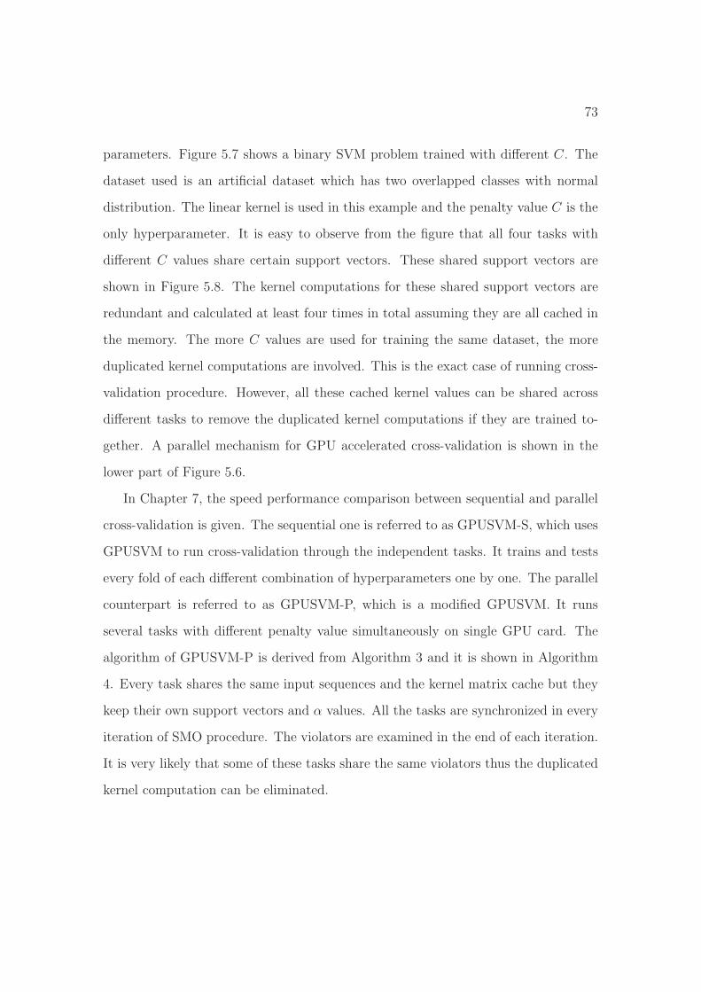
73
parameters. Figure 5.7 shows a binary SVM problem trained with different C. The
dataset used is an artificial dataset which has two overlapped classes with normal
distribution. The linear kernel is used in this example and the penalty value C is the
only hyperparameter. It is easy to observe from the figure that all four tasks with
different C values share certain support vectors. These shared support vectors are
shown in Figure 5.8. The kernel computations for these shared support vectors are
redundant and calculated at least four times in total assuming they are all cached in
the memory. The more C values are used for training the same dataset, the more
duplicated kernel computations are involved. This is the exact case of running cross-
validation procedure. However, all these cached kernel values can be shared across
different tasks to remove the duplicated kernel computations if they are trained to-
gether. A parallel mechanism for GPU accelerated cross-validation is shown in the
lower part of Figure 5.6.
In Chapter 7, the speed performance comparison between sequential and parallel
cross-validation is given. The sequential one is referred to as GPUSVM-S, which uses
GPUSVM to run cross-validation through the independent tasks. It trains and tests
every fold of each different combination of hyperparameters one by one. The parallel
counterpart is referred to as GPUSVM-P, which is a modified GPUSVM. It runs
several tasks with different penalty value simultaneously on single GPU card. The
algorithm of GPUSVM-P is derived from Algorithm 3 and it is shown in Algorithm
4. Every task shares the same input sequences and the kernel matrix cache but they
keep their own support vectors and α values. All the tasks are synchronized in every
iteration of SMO procedure. The violators are examined in the end of each iteration.
It is very likely that some of these tasks share the same violators thus the duplicated
kernel computation can be eliminated.

Figure 5.6: 5-fold cross-validation steps for Gaussian kernels.
74
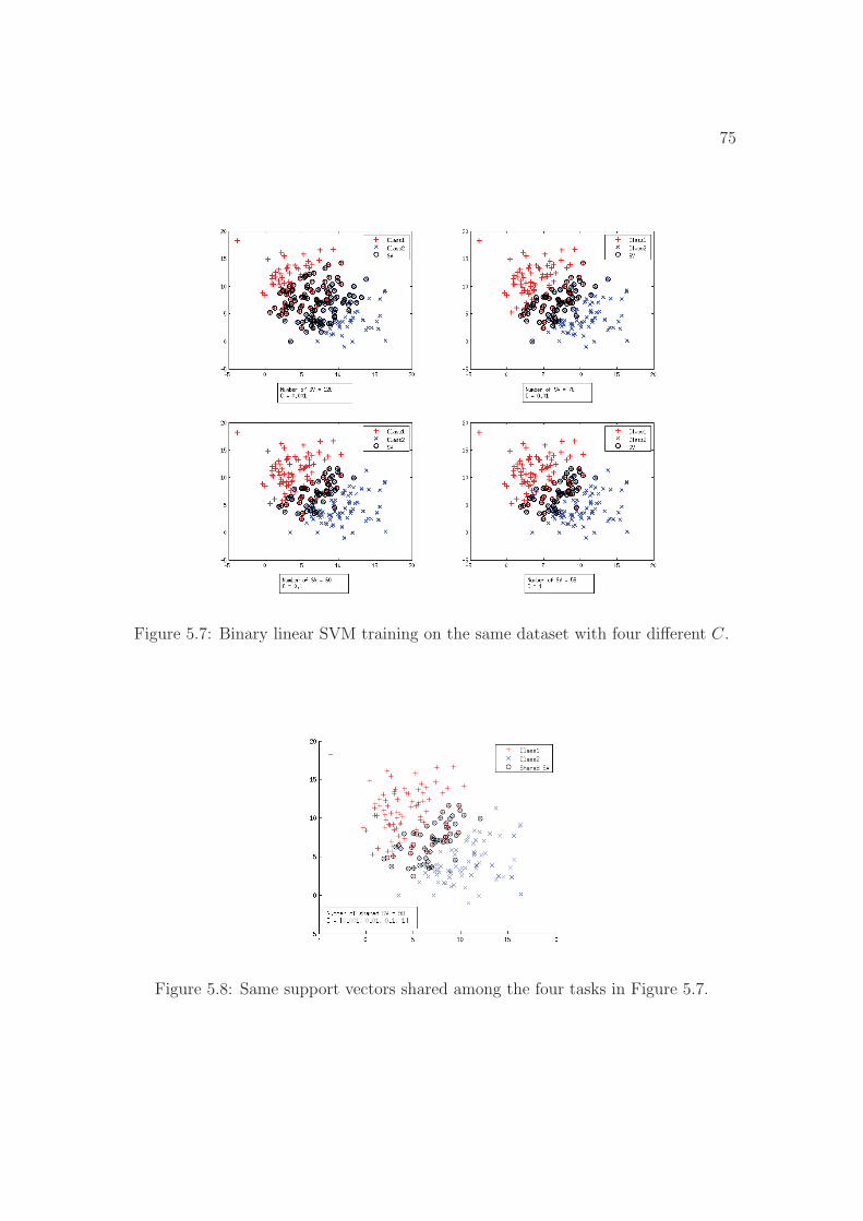
75
Figure 5.7: Binary linear SVM training on the same dataset with four different C.
Figure 5.8: Same support vectors shared among the four tasks in Figure 5.7.

76
Algorithm 4 Parallel Cross Validation.
αki = 0, ek,p
i = −yki (device)
compute bk,pup , bk,p
lo , ik,pup , ik,p
lo (device)compute bk
up, bklo, i
kup, o
klo (host)
while bklo > bk
up + 2τ do∀p, q ∈ [1, k] and p, q ∈ Z
if ipup = iqup ‖ ipup = iqlo ‖ iplo = iqup ‖ iplo = iqlo thenfetch kernel values from GPU memory
elsecompute Kiklo,iklo
, Kikup,ikup, Kikup,iklo
(device)end ifupdate αikup
, αiklo(device)
compute bk,pup , bk,p
lo , ik,pup , ik,p
lo (device)compute bk
up, bklo, i
kup, i
klo (host)
end whileuse αk
i to test the testing setreturn number of misclassified testing samples in a vector for this task C =[C1, ..., Ck]

Chapter 6
A Glance of GPUSVM
This chapter gives the overview of the GPUSVM tool and discusses the implementa-
tion of the software architecture.
6.1 GPUSVM Overview
GPUSVM has three layers. The top layer is a Graphic User Interface (GUI) written
in Java. The GUI offers the user easy access to the tools and parameter setting. It
has three main tabs which are for cross-validation, training and predicting purposes.
They are shown in Figure 6.1, Figure 6.2 and Figure 6.3. The cross-validation interface
allows the user to choose the training file and configure various parameters such as
kernel type and scaling method. User can enter the specific GPU device id in a list to
run the cross-validation procedure on multiple GPUs if available. Our Tesla system
has two Tesla C2070s and six Tesla C2050s, thus the user can use all eight GPUs to
accelerate the cross-validation at the same time. The results of the cross-validation
will be returned as a table showing both number of support vectors and number of
misclassifications for all different combinations of the training parameters. It draws
a 2D surface for Gaussian/polynomial kernel and a curve for linear kernel. Because
77

78
there is only one hyperparameter needed for tuning linear SVM which is the penalty
value C.
Figure 6.1: GPUSVM: cross-validation interface.
6.2 GPUSVM Implementation
The training interface lets the user choose the training file and enter the specific
parameters for a particular kernel. The user is also able to specify a GPU device
to run the training task. After the training procedure is done, a model file will be
generated which contains all the necessary information for making predictions on the
testing datasets. The training file could also be scaled before it is used. Three scaling
methods are offered. Two of them scale the dataset to a value range of [0, 1] or [−1, 1].
The third one scales the dataset with zero mean and standard deviation equal to one.
The scaling information are stored in a separated file, which is used for scaling the
query, i.e. testing, datasets so that the input feature space can be aligned. The

79
Figure 6.2: GPUSVM: training interface.
Figure 6.3: GPUSVM: predicting interface.
predicting interface requires the user to choose the query datasets and the model file
as well as the scaling file. If the scaling is not performed during the training phase,

80
the scaling file will be an empty file. The user can specify the GPU device id for
predicting phase. The result shows the number of misclassifications and the actual
predicting accuracy.
The middle layer of GPUSVM package are several script files written in Python.
Their major tasks are doing file manipulations. The shuffling tool rearranges the
input data sequences randomly which is critical in cross-validation. In each fold
of cross-validation, if the training part does not have equal distributions from all
different classes, it could lead to some bad results. The scaling tool scales the input
dataset according to a particular scaling method or an existing scaling file. The cross-
validation tool slices the input data file to multiple folds and prepare the training
dataset and verification dataset for the SVM solver and predictor. The SVM solver
tool and predictor tool call the actual routine in the bottom layer for training and
predicting purposes.
The bottom layer of GPUSVM package contains only two executable files written
in C on top of CUDA. One is an SVM solver which solves the QP problem in SVM
and generates the model file using GPU. The other one is a predictor which takes in
the query file and a model file generated by the SVM solver to make predictions.

Chapter 7
GPUSVM Accuracy and Speed
Performance on Real World
Datasets
This chapter presents the experimental results achieved by using GPUSVM. The state
of the art LIBSVM tool is used for comparison as the CPU counterpart. The system
hardware configuration is given first and then the characteristics of the benchmarking
datasets used in the tests are listed. The experimental tests focus on the comparison
in terms of both the accuracy and speed performance. They are performed on different
scale of datasets ranging from small number of examples to large number of examples.
The shared kernel cross-validation performance is given in the end of the chapter.
7.1 Host and Device
The GPUSVM tool is developed using CUDA in C/C++. All the experimental tests
are carried out by our latest Tesla server equipped with two Intel Xeon X5680 3.3GHz
six-core CPUs, 96GB ECC DDR3 1333MHz main memory, six Tesla C2050 with 3GB
81

82
GDDR5 memory each and two Tesla C2070 with 6GB GDDR5 memory each. The
storage device is a 128GB SSD with Fedora Core Linux 14 x64 installed. The CUDA
driver and runtime version are both 3.2.
7.2 The Experimental Datasets
This section gives the information of datasets used in the experimental tests. All
datasets used are downloaded either from official LIBSVM [10] website or LIBCVM
[42] website. These datasets can be roughly divided into three different scales de-
pending upon their sample sizes. Datasets which have less than 1000 samples are
classified as small datasets. If the sample size of a dataset is ranging from 1000 to
100000, it is classified as a medium dataset. Datasets are classified as large datasets
if their sample sizes are bigger than 100000. The characteristics of these datasets and
the hyperparameters for the Gaussian RBF kernel are listed in Table 7.1. Several
of them are binary class datasets and the rest are multiclass datasets. Glass, iris,
wine, sonar, breast-cancer, adult datasets are from UCI [43] and heart, letter, shuttle
datasets are from Statlog [44]. Usps is a hand written dataset [45] for text recognition.
Web is web pages text categorization used in [7]. Mnist is another hand written text
recognition dataset used in [46]. There are three large datasets listed at the bottom
of Table 7.1. Usps-ext is the extension dataset of usps. Covtype is from UCI and
face-ext is from MIT. The hyperparameter C is the penalty value and γ is the shape
value of RBF kernel. The best C and γ are found out by using 5-fold cross-validation
on C ∈ {2i, i ∈ [−10, 10]}, γ ∈ {2i, i ∈ [−5, 5]} and they are listed in Table 7.1. The
accuracy and speed performances shown in the following sections use these C and γ
values. The default ε value used in these tests is 0.001.

83
Table 7.1: The experimental datasets and their hyperparameters for the GaussianRBF kernel.
Scale Dataset# of # of # of # of
C γtraining testing feature classdata data
small
glass 214 N/A 9 6 512 2iris 150 N/A 4 3 16 0.5wine 178 N/A 13 3 1 0.25heart 270 N/A 13 2 0.5 0.0625sonar 208 N/A 60 2 4 0.125
breast-cancer 683 N/A 10 2 0.25 0.125
medium
adult 32561 16281 123 2 1 0.0625usps 7291 2007 256 10 128 0.015625letter 15000 5000 16 26 16 8shuttle 43500 14500 9 7 1 1web 49749 14951 300 2 64 8
mnist 60000 10000 780 10 16 0.003906
largeusps-ext 266079 75383 675 2 1 0.03125covtype 500000 81012 54 7 1 1face-ext 489410 24045 361 2 0.001 1
7.3 The Accuracy Comparison Test on Small and
Medium Datasets
Table 7.2 shows the accuracy performance between GPUSVM and LIBSVM on small
and medium datasets. In this test, both methods have very close accuracy perfor-
mance compared to each other. GPUSVM offers as good accuracy as LIBSVM does.
Their final accuracies are slightly different from each other. This is because their
model do not posses exact number of support vectors. Besides, LIBSVM uses double
precision floating points and GPUSVM uses single precision floating points. This
will cause some minor differences in their final α values. GPUSVM does not support
double precision because the speed performance of floating points operations using

84
Table 7.2: The accuracy performance comparison between GPUSVM and LIBSVMon small and medium datasets.
dataset SVMTraining Predicting # ofAccuracy Accuracy support vector
glassLIBSVM 98.5981%
N/A133
GPUSVM 98.1308% 144
irisLIBSVM 98%
N/A25
GPUSVM 98% 27
wineLIBSVM 99.4382%
N/A68
GPUSVM 99.4382% 75
heartLIBSVM 85.1852%
N/A146
GPUSVM 85.1852% 146
sonarLIBSVM 100%
N/A150
GPUSVM 100% 150
breast-cancerLIBSVM 97.2182%
N/A91
GPUSVM 97.2182% 91
adultLIBSVM 85.7928% 85.0132% 11647GPUSVM 85.7928% 85.0193% 11587
uspsLIBSVM 99.9863% 95.6153% 1785GPUSVM 99.9863% 95.715% 1923
letterLIBSVM 100% 96.82% 10726GPUSVM 99.8467% 97.38% 11936
shuttleLIBSVM 99.5149% 99.6069% 3109GPUSVM 99.4736% 99.5655% 3667
webLIBSVM 99.4553% 99.4515% 35231GPUSVM 99.4553% 99.4515% 35220
mnistLIBSVM 99.5917% 98.03% 9738GPUSVM 99.4617% 98.27% 12919
double precision on GPU is significantly lower than using single precision. Using
double precision also requires twice of memory storage space for the same amount of
data compared to using single precision. And this will bring memory limits to the
GPUSVM on solving large datasets problems. The accuracy performance of LIBSVM
has shown that it does not benefit from using double precision. Thus the GPUSVM
is designed using single precision which achieves similar accuracy performance and

85
emphasizes more on speed and solving large scale problems. For binary class datasets,
GPUSVM has almost identical number of support vectors as LIBSVM does. LIB-
SVM implements OVO and GPUSVM uses OVA approach for multiclass datasets
thus their number of support vectors differ from each other. LIBSVM uses a working
set method which solves a QP problem with the size larger than two. GPUSVM also
uses an analytic method to iteratively solve the QP problem with the working set size
fixed at two.
7.4 The Speed Performance Comparison Test on
Small and Medium Datasets
The following tests shown in Table 7.3 and Table 7.4 are the speed performance
between LIBSVM and GPUSVM in both training and predicting phases for small and
medium datasets. Small datasets do not have testing set therefore only the training set
is used for prediction. The performance of LIBSVM using one core of Xeon processor
is set as the base line. It is compared with LIBSVM using all 12 cores from two
Xeon CPUs with LIBSVM’s built in OpenMP feature enabled. The total number
of threads is set at 12 to extract the maximum performance of multi-core CPU.
GPUSVM using one Tesla C2050/C2070 is also listed as the comparison reference
to show the speedup. All GPU devices used for tests have the Error Correction
Code (ECC) function disabled. This will free more device memory to the application
programs. It is easy to see that whether using GPU or multi-core CPU does not
bring any performance gain for solving small SVM classification problem due to the
overhead of using OpenMP and CUDA. Besides, the training time and predicting
time on small datasets are trivial. On the other hand, GPUSVM shows much better
performance on medium datasets and it achieves a speedup of 2.27x - 77x compared

86
to standard LIBSVM. Tesla C2070 is generally faster than Tesla C2050 because of
the doubled device memory.
Table 7.3: The speed performance comparison between GPUSVM and LIBSVM onsmall datasets.
dataset SVM ProcessorTraining
SpeedupPredicting
SpeedupTime Time
glassLIBSVM
Xeon 1-core 0.008s 1x 0.004s 1xXeon 12-core 0.010s 0.8x 0.005s 0.8x
GPUSVMTesla C2050 3.759s 0.0021x 0.009s 0.4444xTesla C2070 2.32s 0.0035x 0.008s 0.5x
irisLIBSVM
Xeon 1-core 0.002s 1x 0.002s 1xXeon 12-core 0.003s 0.6667x 0.004s 0.5x
GPUSVMTesla C2050 1.305s 0.0015x 0.006s 0.3333xTesla C2070 1.284s 0.0016x 0.006s 0.3333x
wineLIBSVM
Xeon 1-core 0.003s 1x 0.003s 1xXeon 12-core 0.004s 0.75x 0.005s 0.6x
GPUSVMTesla C2050 1.567s 0.0019x 0.008s 0.375xTesla C2070 1.055s 0.0028x 0.007s 0.4286x
heartLIBSVM
Xeon 1-core 0.006s 1x 0.005s 1xXeon 12-core 0.005s 1.2x 0.006s 0.8333x
GPUSVMTesla C2050 1.03s 0.0058x 0.01s 0.5xTesla C2070 1.048s 0.0057x 0.01s 0.5x
sonarLIBSVM
Xeon 1-core 0.014s 1x 0.011s 1xXeon 12-core 0.011s 1.2727x 0.011s 1x
GPUSVMTesla C2050 1.383s 0.0101x 0.009s 1.2222xTesla C2070 1.645s 0.0085x 0.009s 1.2222x
LIBSVMXeon 1-core 0.008s 1x 0.006s 1x
breast Xeon 12-core 0.006s 1.3333x 0.012s 0.5xcancer
GPUSVMTesla C2050 1.352s 0.0059x 0.025s 0.24xTesla C2070 1.395s 0.0057x 0.022s 0.2727x
The speed performance of OpenMP enabled LIBSVM is quite good on medium
size datasets. This is due to the shared memory system setting. All threads resided
in the CPU can access the large main memory. And most of the kernel values can
be cached in the main memory. However, this performance is strictly limited by the

87
Table 7.4: The speed performance comparison between GPUSVM and LIBSVM onmedium datasets.
dataset SVM ProcessorTraining
SpeedupTesting
SpeedupTime Time
adultLIBSVM
Xeon 1-core 60.634s 1x 20.273s 1xXeon 12-core 8.998s 6.7386x 2.216s 9.1485x
GPUSVMTesla C2050 8.644s 7.0145x 0.697s 29.0861xTesla C2070 7.636s 7.9405x 0.649s 31.2373x
uspsLIBSVM
Xeon 1-core 4.901s 1x 2.113s 1xXeon 12-core 1.331s 3.6822x 0.446s 4.7377x
GPUSVMTesla C2050 3.005s 1.6309x 0.088s 24.0114xTesla C2070 2.158s 2.2711x 0.081s 26.0864x
letterLIBSVM
Xeon 1-core 37.768s 1x 4.666s 1xXeon 12-core 11.902s 3.1712x 1.88s 2.4819x
GPUSVMTesla C2050 11.318s 3.3370x 0.465s 10.0344xTesla C2070 10.554s 3.5785x 0.445s 10.4854x
shuttleLIBSVM
Xeon 1-core 9.379s 1x 2.402s 1xXeon 12-core 2.047s 4.5818x 0.642s 3.7414x
GPUSVMTesla C2050 3.267s 2.8708x 0.573s 4.192xTesla C2070 2.238s 4.1908x 0.526s 4.5665x
webLIBSVM
Xeon 1-core 1450.933s 1x 59.278s 1xXeon 12-core 199.784s 7.2625x 6.819s 8.6931x
GPUSVMTesla C2050 94.317s 15.3836x 1.267s 46.7861xTesla C2070 71.291s 20.3523x 1.217s 48.7083x
mnistLIBSVM
Xeon 1-core 256.579s 1x 86.559s 1xXeon 12-core 64.04s 4.0065x 10.183s 8.5003x
GPUSVMTesla C2050 58.308s 4.4004x 1.154s 75.0078xTesla C2070 39.552s 6.4871x 1.124s 77.0098x
number of CPUs and the cores of each CPU on the motherboard. That means the
maximum performance of CPU in this workstation is achieved. Using any number
of threads other than 12 will not gain any benefit. On the other hand, the potential
of using GPU is huge since there is only one GPU device involved in the current
testing. Properly developed multi-GPU model is expected to bring dramatic speed
improvement.

88
7.5 Experimental Results for Different Epsilon on
Medium Datasets
In this part of tests, various ε values are used to find out the impacts on both accuracy
and speed performance of changing the value of ε. The ε value is used as the converging
criteria during the iterative learning process in the SMO procedure. In theory, the
smaller the ε value is, the longer time the convergence will be likely to take for each
iteration. The recommended ε value is 0.001 which has been mentioned in Section 5.
In the following tests, the ε values used are 0.0001, 0.001, 0.01 and 0.1. The accuracy
is measured for predicting datasets. The time cost is measured for training phase.
The medium datasets are used due to their varieties.
Figure 7.1 shows that all datasets have close accuracy performance on different ε
values except the usps dataset. The accuracy of usps dataset has a drop on both very
small and very large ε values. The largest ε value used on usps dataset produces an
accuracy which is significantly lower than any other ε values do.
Figure 7.2 presents the total number of support vectors found during the training
phase for different ε values. The web dataset is the only one which has much smaller
number of support vectors when it is trained by using the largest ε value. All other
datasets get close number of support vectors by using different ε values. Considering
the accuracy performance shown in Figure 7.1, web dataset actually requires less
number of support vectors to achieve its best accuracy.
Figure 7.3 shows the time cost in seconds for the training phase by using different
ε values. All datasets shows a decline of time cost when the ε increases except usps.
Usps has slight increase of time cost when ε increases. It is expected that a larger
epsilon value should make the converging procedure faster.
It is obvious that different ε values do bring some impacts for both accuracy

89
Figure 7.1: The accuracy performance for different ε values on medium datasets.
and speed performances. These impacts vary case by case on individual datasets.
However, it is also clear to see that the default ε value can always produce good
enough results.
7.6 Experimental Results on Large Datasets
In this test, both the accuracy performance and speed performance comparison be-
tween GPUSVM and LIBSVM are measured on large datasets. Table 7.5 shows the
accuracy comparison and the number of support vectors acquired during the training
phase. The hyperparameters used in the tests are listed in Table 7.1. These accura-

90
Figure 7.2: The number of support vectors for different ε values on medium datasets.
cies are for testing data given in Table 7.1. For the binary class usps-ext and face-ext
datasets, GPUSVM and LIBSVM achieve exactly the same accuracy. LIBSVM per-
forms slightly better on the multiclass covtype dataset, which might be due to the
performance difference between OVO and OVA.
Table 7.6 shows the training time cost, the predicting time cost and the relative
speedups compared to the LIBSVM using 1 core. The training time cost is also
shown as a graphic representation in Figure 7.4. GPUSVM outperforms standard
LIBSVM approximately two orders of magnitude and OpenMP enabled LIBSVM
about one order of magnitude. This is very impressive speed improvement and it
shows that GPUSVM is more suitable for large scale datasets. Figure 7.5 is the time

91
Figure 7.3: The speed performance for different ε values on medium datasets.
Table 7.5: The accuracy performance comparison between CPU and GPU on largedatasets.
Dataset SVMTesting # of
Accuracy support vector
usps-extLIBSVM 99.2332% 39570GPUSVM 99.2332% 38598
covtypeLIBSVM 80.5028% 246444GPUSVM 80.3362% 267373
face-extLIBSVM 98.037% 52488GPUSVM 98.037% 34992

92
cost comparison of predicting phase. GPUSVM is blazing fast which is about 16 times
faster than OpenMP enabled LIBSVM and 380 times faster than standard LIBSVM.
Table 7.6: The speed performance comparison between CPU and GPU on largedatasets.
Dataset SVMTraining
SpeedupTesting
SpeedupTime Time
usps-extLIBSVM (Xeon 1-core) 1511.9m 1x 190.7m 1xLIBSVM (Xeon 12-core) 66.4m 22.8x 8.4m 22.7xGPUSVM (Tesla C2070) 8.4m 180x 0.5m 381.4x
covtypeLIBSVM (Xeon 1-core) 1347.7m 1x 198m 1xLIBSVM (Xeon 12-core) 59m 22.84x 8.7 22.76xGPUSVM (Tesla C2070) 19.4m 69.5x 0.7m 282.9x
face-extLIBSVM (Xeon 1-core) 6522.8m 1x 195m 1xLIBSVM (Xeon 12-core) 286.5m 22.77x 8.5m 22.9xGPUSVM (Tesla C2070) 5.3m 1230.7x 0.3m 650x
Figure 7.4: Training time comparison between GPUSVM and LIBSVM on largedatasets.

93
Figure 7.5: Predicting time comparison between GPUSVM and LIBSVM on largedatasets.
7.7 The Cross Validation Performance Compari-
son Using Single GPU
One of major contributions of this dissertation is using shared kernel matrix across
multiple training tasks during the cross-validation procedure. Each training task with
its own hyperparameter shares the kernel matrix cached in the GPU memory. Thus
many duplicated kernel computations can be eliminated so that the training time
cost can be shortened. Adult and web datasets are used for measuring the shared
kernel cross-validation speed performance. Table 7.7 shows the comparison of the
training time cost between GPUSVM-S, GPUSVM-P and LIBSVM. GPUSVM-S is
the single task training as mentioned before and it trains a pair of C and γ one by
one on GPU. It basically calls GPUSVM tool directly. GPUSVM-P is a modified
GPUSVM tool which uses the shared kernel matrix to train all C and one γ to-

94
gether. LIBSVM trains a pair of C and γ one by one which is the same as what
GPUSVM-S does. For adult dataset, the training parameters are γ = 0.0625 and
C ∈ {0.125, 0.25, 0.5, 1, 2, 4, 8, 16, 32, 64}. For web dataset, the training parameters
are γ = 8 and C ∈ {0.125, 0.25, 0.5, 1, 2, 4, 8, 16, 32, 64}. The performance of LIBSVM
is set as the benchmark baseline. GPUSVM-P is 10 times faster on adult dataset and
almost 100 times faster on web dataset for SVM training.
Table 7.7: The speed performance comparison among GPUSVM-S, GPUSVM-P andLIBSVM.
Dataset SVM Training time Speedup
adultLIBSVM 1601.37s 1x
GPUSVM-S 309.91s 5.2xGPUSVM-P 155.42s 10.3x
webLIBSVM 12198.3s 1x
GPUSVM-S 564.16s 21.6xGPUSVM-P 123.36s 98.9x
In order to analyze the performance result in more detail, Figure 7.6 shows the
independent task comparison between LIBSVM and GPUSVM-S. Both of them are
measured with 10 pairs of different combinations of C and γ values in 10 tasks.
GPUSVM-S shows good speed improvement on every independent task. The total
number of support vectors of GPUSVM-S and LIBSVM is very close in each task,
which guarantees the accuracy performance. The support vectors and their related
α obtained by GPUSVM-P are identical to GPUSVM-S. The total number of ker-
nel computations are shown in Figure 7.7. The duplicated kernel computations in
GPUSVM-S lead to a longer training time compared to GPUSVM-P.

Figure 7.6: Independent task comparison on speed performance and number of sup-port vectors between GPUSVM and LIBSVM.
Figure 7.7: Total number of kernel computations for GPUSVM-S and GPUSVM-P.
95

Chapter 8
Conclusions and Future Work
This dissertation covers the fields of machine learning, i.e. data mining. In particular,
it contributes to the speeding up the approaches, algorithms and software for learning
from large datasets. It is focused primarily on the classification (pattern recognition)
algorithms but the ideas and software developed can readily be extended to solving
regression (high-dimensional functions approximation) tasks too. All the algorithms
are implemented on GPGPUs but they can be extended to other parallel computing
environment.
The first, massive calculation, problem to be solved was a calculation of distance
matrix for large datasets. A general CUDA based distance calculation method is
proposed which works for three different distance kernels including weighted Euclidean
distance, cosine similarity and weighted Manhattan distance. It achieves roughly
5 times speedup on Euclidean distance calculation compared to the fastest CPU’s
algorithms. Several parallel sorting algorithms are also compared and they have their
own advantages and disadvantages according to different scenarios. By combining
the parallel distance matrix computation and parallel sorting algorithms together, an
efficient CUDA based parallel k-NNs search tool, GPUKNN, is developed to accelerate
the time consuming k-NNs search procedure. The results obtained have shown that
96

97
GPUKNN is faster than VG-KNN, which has been considered as being many times
faster than other CPU based k-NNs search algorithms.
A parallel processing algorithm for SVM training on GPGPUs, which uses a paral-
lel SMO is also proposed and implemented in this dissertation. The related software
package GPUSVM is developed on top of CUDA platform. Although GPUSVM
does not have a rich feature set like LIBSVM does, it offers enough capability to
process real-world datasets. It supports multiclass classification, three popular ker-
nel functions for SVM training, cross-validation and double (nested) cross-validation.
GPUSVM achieves very close accuracy performance as LIBSVM does since they both
use working set technique for solving QP problem. For small datasets, GPUSVM does
not benefit from its parallel architecture since the training time is trivial. However,
when it comes to the medium and large datasets, GPUSVM shows the superior per-
formance in terms of speed. The time cost by using GPUSVM is from one order of
magnitude to three orders of magnitude (10 to 1000) times smaller compared to LIB-
SVM’s one. The novel cross-validation tool implemented in GPUSVM using shared
kernel matrix has much better speed performance than standard cross-validation pro-
cedure due to the heavily reduced amount of kernel computations. This method may
be less capable of solving large datasets compared to the standard one because of the
memory limitations. The cross-validation can always be accelerated by using multiple
GPU devices.
GPUs have brought an opportunity of accelerating many applications to solve
various problems. Although GPUs can generally improve the speed performance
compared to classic sequential algorithms, there are many different factors which all
have more or less impacts on how much improvement one can achieve with the help
of GPUs. For example, the Amdahl’s law decides the maximal possible acceleration
brought by parallel processing for a certain problem. Thus, it is important to dive

98
deeper into understanding both how CUDA model works and what special features
are offered by CUDA. It is even more important to discover the parallelism in a
certain problem and how to use the features offered by CUDA to solve it. The major
future work of this dissertation can be extending the current algorithm to solving
problems with ultra-large datasets. The recent release of CUDA 4.0 introduces new
features like Unified Virtual Addressing. This feature can connect all the devices
memory from different GPU cards together, and in this way every GPU card can
bypass the CPU and main memory to access the global memory from other cards.
Thus, an ultra-large dataset will be able to fit into the memory of multiple GPU
cards and the memory limitation of one single card will be resolved. There are
a few more possible extensions of this dissertation in future such as tuning cross-
validation and adding support of solving regression problems. Tuning cross-validation
is an important procedure because people always use cross-validation to find the
best hyperparameter for the training dataset and these hyperparameters are used
for generating the SVM model. Standard cross-validation performs a grid search on
a series of hyperparameters. This could lead to a very long training time due to
the improper combinations of hyperparameters used. One possible method which
can accelerate the search of the best hyperparameters is automatic tuning. Adding
regression support is another good extension because SVM is not only very popular for
its classification performance, but it also has good performance in solving regression
problems. It is expected that GPUs can bring significant speed improvement in
solving regression problems.

List of References
[1] V. Kecman and J. P. Brooks, “Locally linear support vector machines and other
local models,” in Neural Networks (IJCNN), The 2010 International Joint Con-
ference on, pp. 1–6, July 2010.
[2] T. Yang and V. Kecman, “Adaptive local hyperplane classification,” Neurocom-
puting, vol. 71, no. 13-15, pp. 3001–3004, 2008.
[3] V. N. Vapnik, The Nature of Statistic Learning Theory. New York: Springer-
Verlag, 1995.
[4] T.-M. Huang, V. Kecman, and I. Kopriva, “Iterative single data algorithm for
kernel machines from huge data sets: Theory and performance,” in Kernel Based
Algorithms for Mining Huge Data Sets, vol. 17 of Studies in Computational In-
telligence, pp. 61–95, Springer Berlin / Heidelberg, 2006.
[5] E. Osuna, R. Freund, and F. Girosi, “An improved training algorithm for sup-
port vector machines,” in Neural Networks for Signal Processing [1997] VII.
Proceedings of the 1997 IEEE Workshop, pp. 276–285, September 1997.
[6] T. Joachims, Making large-scale support vector machine learning practical,
pp. 169–184. Cambridge, MA, USA: MIT Press, 1999.
99

100
[7] J. C. Platt, Fast training of support vector machines using sequential minimal
optimization, pp. 185–208. Cambridge, MA, USA: MIT Press, 1999.
[8] C. B. S. S. Keerthi, S. K. Shevade and K. R. K. Murthy, “Improvements to
platt’s smo algorithm for svm classifier design,” Neural Computation, vol. 13,
pp. 637–649, March 2001.
[9] P.-H. C. R.-E. Fan and C.-J. Lin, “Working set selection using second order
information for training support vector machines,” Journal of Machine Learning
Research, vol. 6, pp. 1889–1918, December 2005.
[10] C.-C. Chang and C.-J. Lin, LIBSVM: a library for support vector machines,
2001. Software available at http://www.csie.ntu.edu.tw/~cjlin/libsvm.
[11] S. B. R. Collobert and Y. Bengio, “A parallel mixture of svms for very large
scale problems,” Neural Computation, vol. 14, no. 5, pp. 1105–1114, 2002.
[12] A. K. J.-X. Dong and C.-Y. Suen, “A fast parallel optimization for training sup-
port vector machine,” in Machine Learning and Data Mining in Pattern Recog-
nition, vol. 2734 of Lecture Notes in Computer Science, pp. 96–105, Springer
Berlin / Heidelberg, 2003.
[13] G. Zanghirati and L. Zanni, “A parallel solver for large quadratic programs in
training support vector machines,” Parallel Computing, vol. 29, pp. 535–551,
April 2003.
[14] C.-K. S. G.-B. Huang, K. Z. Mao and D.-S. Huang, “Fast modular network imple-
mentation for support vector machines,” Neural Networks, IEEE Transactions
on, vol. 16, pp. 1651–1663, November 2005.
[15] L. J. Cao, S. S. Keerthi, C.-J. Ong, J. Q. Zhang, U. Periyathamby, X. J. Fu, and
H. P. Lee, “Parallel sequential minimal optimization for the training of support

101
vector machines,” Neural Networks, IEEE Transactions on, vol. 17, pp. 1039–
1049, July 2006.
[16] H. P. Graf, E. Cosatto, L. Bottou, I. Durdanovic, and V. Vapnik, “Parallel sup-
port vector machines: The cascade svm,” in In Advances in Neural Information
Processing Systems, pp. 521–528, MIT Press, 2005.
[17] B. Catanzaro, N. Sundaram, and K. Keutzer, “Fast support vector machine
training and classification on graphics processors,” in Proceedings of the 25th
international conference on Machine learning, ICML ’08, (New York, NY, USA),
pp. 104–111, ACM, 2008.
[18] S. Herrero-Lopez, J. R. Williams, and A. Sanchez, “Parallel multiclass classifica-
tion using svms on gpus,” in Proceedings of the 3rd Workshop on General-Purpose
Computation on Graphics Processing Units, GPGPU ’10, (New York, NY, USA),
pp. 2–11, ACM, 2010.
[19] G. Fung and O. L. Mangasarian, “Proximal support vector machine classifiers,”
in Proceedings of the seventh ACM SIGKDD international conference on Knowl-
edge discovery and data mining, KDD ’01, (New York, NY, USA), pp. 77–86,
ACM, 2001.
[20] O. L. Mangasarian and E. W. Wild, “Multisurface proximal support vector ma-
chine classification via generalized eigenvalues,” Pattern Analysis and Machine
Intelligence, IEEE Transactions on, vol. 28, pp. 69–74, January 2006.
[21] N. Segata and E. Blanzieri, “Fast and scalable local kernel machines,” Journal
of Machine Learning Research, pp. 1883–1926, Aug 2010.

102
[22] E. Blanzieri and F. Melgani, “Nearest neighbor classification of remote sensing
images with the maximal margin principle,” Geoscience and Remote Sensing,
IEEE Transactions on, vol. 46, pp. 1804–1811, June 2008.
[23] H. Samet, “K-nearest neighbor finding using maxnearestdist,” Pattern Analysis
and Machine Intelligence, IEEE Transactions on, vol. 30, pp. 243–252, February
2008.
[24] D.-J. Chang, N. A. Jones, D. Li, M. Ouyang, and R. K. Ragade, “Compute pair-
wise euclidean distances of data points with gpus,” in Computational Biology and
Bioinformatics, 2008. CBB ’08. IASTED International Symposium, November
2008.
[25] Q. Li, V. Kecman, and R. Salman, “A chunking method for euclidean distance
matrix calculation on large dataset using multi-gpu,” in Machine Learning and
Applications (ICMLA), 2010 Ninth International Conference on, pp. 208–213,
December 2010.
[26] V. Garcia, E. Debreuve, and M. Barlaud, “Fast k nearest neighbor search using
gpu,” in Computer Vision and Pattern Recognition Workshops, 2008. CVPRW
’08. IEEE Computer Society Conference on, pp. 1–6, 23-28 2008.
[27] Q. Li, R. Salman, and V. Kecman, “Accelerating weighted euclidean distance and
cosine similarity calculation using gpu,” in Intelligent Information Technology
Application, 2010 4th International Conference on, pp. 108–111, Nov 2010.
[28] M. P. I. Forum, “Mpi: A message-passing interface standard, version 2.2,” 2009.
http://www.mpi-forum.org/docs/mpi-2.2/mpi22-report.pdf.
[29] O. A. R. Board, “Openmp specifications version 3.0,” May 2008. http://www.
openmp.org/mp-documents/spec30.pdf.

103
[30] K. Group, “The opencl specification version 1.0,” 2009. http://www.khronos.
org/registry/cl/specs/opencl-1.0.29.pdf.
[31] NVIDIA, CUDA CUBLAS Library, June 2007.
[32] J. Cohen, “Cuda libraries and tools,” 2009.
[33] R. Pike, S. Dorward, R. Griesemer, and S. Quinlan, “Interpreting the data:
Parallel analysis with sawzall,” Sci. Program., vol. 13, no. 4, pp. 277–298, 2005.
[34] N. Satish, M. Harris, and M. Garland, “Designing efficient sorting algorithms for
manycore gpus,” in Parallel Distributed Processing, 2009. IPDPS 2009. IEEE
International Symposium on, pp. 1–10, May 2009.
[35] D. Cederman and P. Tsigas, “Gpu-quicksort: A practical quicksort algorithm
for graphics processors,” J. Exp. Algorithmics, vol. 14, pp. 4:1.4–4:1.24, January
2010.
[36] C. Cortes and V. Vapnik, “Support-vector networks,” Machine Learning, vol. 20,
pp. 273–297, 1995.
[37] K. Crammer and Y. Singer, “On the algorithmic implementation of multiclass
kernel-based vector machines,” Journal of Machine Learning Research, vol. 2,
pp. 265–292, March 2002.
[38] U. H.-G. Kreßel, Pairwise classification and support vector machines, pp. 255–
268. Cambridge, MA, USA: MIT Press, 1999.
[39] R. Rifkin and A. Klautau, “In defense of one-vs-all classification,” Journal of
Machine Learning Research, vol. 5, pp. 101–141, Jan. 2004.

104
[40] T. fan Wu, C.-J. Lin, and R. C. Weng, “Probability estimates for multi-class clas-
sification by pairwise coupling,” Journal of Machine Learning Research, vol. 5,
pp. 975–1005, 2003.
[41] R. Rifkin and A. Klautau, “In defense of one-vs-all classification,” Journal of
Machine Learning Research, vol. 5, pp. 101–141, 2004.
[42] I. W. Tsang, A. Kocsor, and J. T. Kwok, LibCVM Toolkit, 2011. Software
available at http://c2inet.sce.ntu.edu.sg/ivor/cvm.html.
[43] A. Frank and A. Asuncion, “UCI machine learning repository,” 2010.
[44] LIACC, “Statlog datasets,” 2010.
[45] J. Hull, “A database for handwritten text recognition research,” Pattern Analysis
and Machine Intelligence, IEEE Transactions on, vol. 16, pp. 550–554, may 1994.
[46] Y. Lecun, L. Bottou, Y. Bengio, and P. Haffner, “Gradient-based learning applied
to document recognition,” Proceedings of the IEEE, vol. 86, pp. 2278–2324, nov
1998.

105
Vita
Qi Li was born on Aug 23rd, 1985 in China. He received his Bachelor of Science
in Electrical Engineering from Beijing University of Posts and Telecommunications
in 2007 and Master of Science in Computer Science from Virginia Commonwealth
University in 2008. His research interests include machine learning, high performance
computing and parallel computing using Graphic Processing Units. Previously, he
also worked on embedded system design area including micro-controller programming
and circuit layout.
![Centre de médecine chinoisecentredemedecinechinoise.com/wp-content/uploads/2012/06/fondemen… · [qi heng zhi fu]. 2 [dui li], , transformation ... [liu yin xie qi] : le Vent [feng],](https://img.pdfslide.net/doc/110x75/5aa77aa27f8b9ac5648c280e/centre-de-mdecine-chinoisecent-qi-heng-zhi-fu-2-dui-li-transformation.jpg)