Embed Size (px)
Citation preview
QoS AWARE DATA-PATH ROUTING IN
DWDM/GMPLS NETWORK
Suraj Kumar NaikRoll No: 209EC1112
Department of Electronics and Communication Engineering
National Institute of Technology, Rourkela
Rourkela, Odisha, 769 008, India
MAY 2011
QoS AWARE DATA-PATH ROUTING IN
DWDM/GMPLS NETWORK
A thesis submitted in partial fulfillment
of the requirements for the degree of
Master of Technology
in
Electronics and Communication Engineering
by
Suraj Kumar Naik(Roll No: 209EC1112)
Department of Electronics and Communication Engineering
National Institute of Technology, Rourkela
Rourkela, Odisha, 769 008, India
May 2011
QoS AWARE DATA-PATH ROUTING IN
DWDM/GMPLS NETWORK
A Technical Report submitted in partial fulfillment
of the requirements for the degree of
Master of Technology
in
Electronics and Communication Engineering
by
Suraj Kumar Naik(Roll No: 209EC112)
under the guidance of
Prof. Santos Kumar Das
Department of Electronics and Communication Engineering
National Institute of Technology, Rourkela
Rourkela-769 008, Odisha, India
May 2011

Dedicated to my parents
Department of Electronics and Comm EngineeringNational Institute of Technology, RourkelaRourkela-769 008, Odisha, India.
Certificate
This is to certify that the work done for the direction of thesis entitled QoS AWARE
DATA-PATH ROUTING IN DWDM/GMPLS NETWORK submitted by Suraj Ku-
mar Naik in partial fulfillment of the requirements for the award of Master Of Technol-
ogy in Electronic and Communication Engineering with specialization in Telematics
and Signal Processing, at National Institute of Technology Rourkela is an authentic
work carried out by him under my supervision and guidance.
To the best of my knowledge, the matter embodied in the thesis has not been sub-
mitted to any other University/Institute for the award of any Degree or Diploma.
Place: NIT Rourkela Santos Kumar DasDate: 25 May 2011 Professor
Dept. of ECENIT, Rourkela
Acknowledgment
My first thanks are to the Almighty God, without whose blessings I wouldn’t have been
writing this “acknowledgments”.
I am deeply indebted to Prof. Santos Kumar Das, Dept. of ECE, my supervisor on
this project, for consistently providing me with the required guidance to help me in the
timely and successful completion of this project. His advices have value lasting much
beyond this project. I consider it a blessing to be associated with him. Also I am very
thankful to him for reviewing my report.
I would like to express my humble respects to Prof. G. S. Rath, Prof. S.K.Patra,
Prof. K. K. Mahapatra, Prof. S. Meher, Prof. P. Singh, Prof. S. K. Behera, Prof. D.P.
Acharya, Prof. S. Ari, and Prof. A. K. Sahoo for teaching me and also helping me how
to learn. I would like to thanks all faculty members of ECE department for their help
and guidance. They have been great sources of inspiration to me and I thank them from
the bottom of my heart.
I would like to thank all my friends and especially my classmates for all the thought-
ful and mind stimulating discussions we had, which prompted us to think beyond the
obvious. I have enjoyed their companionship so much during my stay at NIT, Rourkela.
Finally, I thank my parents and all my family members for their unlimited support
and strength. Without their dedication and dependability, I could not have pursued my
M.Tech. degree at the National Institute of Technology Rourkela.
Suraj Kumar Naik
ii
Abstract
Quality of Service Routing is at present an active and remarkable research area,
since most emerging network services require specialized Quality of Service (QoS)
functionalities that cannot be provided by the current QoS-unaware routing protocols.
Now-a-days QoS based data routing is a demanding factor for telecommunication clients.
In order to provide better QoS, the service provider network needs to have dynamic
light-path provisioning technique. This technique can help to change the quality of
the light-path dynamically based on existing traffic load and clients QoS requirements,
which can be solved by properly designing Generalized Multi-Protocol Label Switch-
ing (GMPLS) capable hybrid network. This network is the combination of physical
layer as well as network layer information. In optical networks, physical layer impair-
ments (PLIs) incurred by non-ideal optical transmission media, accumulates along the
optical path. The overall effect of PLIs determines the feasibility of the light-paths.
Hence it is important to understand the process that provide PLI information to the con-
trol plane protocols and use this information efficiently to compute feasible routes and
wavelengths. Thus, a successful and wide deployment of the most novel network ser-
vices demands that we thoroughly understand the essence of QoS Routing dynamics,
and also that the proposed solutions to this complex problem should be indeed feasible
and affordable.
Keywords: Q-Factor, Bandwidth, Delay, General Purpose Router, Traffic Control Man-
ager, Quality of Service.
iii
List of Abbreviations
QoS Quality of ServiceTCM Traffic Control ManagerMPLS Multi Protocol Label SwitchingGMPLS Generalized Multi Protocol Label SwitchingWDM Wavelength Division MultiplexingDWDM Dense Wavelength Division MultiplexingIP Internet ProtocolRSVP Resource Reservation Setup ProtocolIETF Internet Engineering Task ForceLSP Label Switched PathPON Passive Optical NetworkLSP Label Switching PathGPR General Purpose RouterSAN Storage Area NetworkATM Asynchronous Transfer ModeUMTS Universal Mobile Telecommunication SystemOXCs Optical Cross ConnectsOADM Optical Add-Drop Multiplexer
iv

List of Symbols
= Equalityλ Wavelength∏
Product∑Summation
δ Pulse Bodening Factor∀ For All
v
Contents
Certificate i
Acknowledgement ii
Abstract iii
List of Abbreviations iv
List of Symbols v
List of Figures viii
List of Tables x
1 Introduction 2
1.1 Motivation . . . . . . . . . . . . . . . . . . . . . . . . . . . . . . . . . 3
1.2 Proposed Work . . . . . . . . . . . . . . . . . . . . . . . . . . . . . . 4
1.3 Objective of the Thesis . . . . . . . . . . . . . . . . . . . . . . . . . . 4
1.4 Organization of rest of the report . . . . . . . . . . . . . . . . . . . . . 4
2 WDM/GMPLS 7
2.1 Basic Concepts . . . . . . . . . . . . . . . . . . . . . . . . . . . . . . 8
2.1.1 Optical Networks . . . . . . . . . . . . . . . . . . . . . . . . . 8
2.1.2 Wavelength Division Multiplexing (WDM) . . . . . . . . . . . 9
2.1.3 Dense Wavelength Division Multiplexing (DWDM) . . . . . . 11
2.2 Multi Protocol Label Switching (MPLS) . . . . . . . . . . . . . . . . . 13
2.2.1 MPLS Layering Structure . . . . . . . . . . . . . . . . . . . . 13
2.2.2 Benefits of MPLS . . . . . . . . . . . . . . . . . . . . . . . . 14
2.2.3 Notation and Definitions . . . . . . . . . . . . . . . . . . . . . 15
2.2.4 MPLS Labels . . . . . . . . . . . . . . . . . . . . . . . . . . . 15
2.2.5 MPLS operations . . . . . . . . . . . . . . . . . . . . . . . . . 17
2.3 Generalised Multi Protocol Label Switching (GMPLS) . . . . . . . . . 17
vi
2.3.1 Routing Protocol . . . . . . . . . . . . . . . . . . . . . . . . . 18
2.3.2 Signaling Protocol . . . . . . . . . . . . . . . . . . . . . . . . 19
2.3.3 Link Management Protocol . . . . . . . . . . . . . . . . . . . . 19
3 System Design 22
3.1 System Model . . . . . . . . . . . . . . . . . . . . . . . . . . . . . . . 22
3.2 Control Plane Protocol and TCM Algorithm . . . . . . . . . . . . . . . 24
3.3 Problem Formulation . . . . . . . . . . . . . . . . . . . . . . . . . . . 25
3.3.1 Bandwidth Model . . . . . . . . . . . . . . . . . . . . . . . . 26
3.3.2 Delay model . . . . . . . . . . . . . . . . . . . . . . . . . . . 26
3.3.3 Q-Factor Model . . . . . . . . . . . . . . . . . . . . . . . . . . 27
3.4 TCM Mechanism for Light-Path Provisioning . . . . . . . . . . . . . . 28
3.4.1 Light-Path provisioning based on only Bandwidth and Delay . . 28
3.4.2 Light-Path provisioning based on Q-Factor . . . . . . . . . . . 28
3.4.3 De- provisioning based on Q-Factor based on Required Q-Factor 28
3.5 Algorithm for Light-Path Selection . . . . . . . . . . . . . . . . . . . . 29
3.5.1 Algorithm for light-path selection based on Bandwidth and Delay 29
3.5.2 Algorithm for light-path selection based on Q-Factor . . . . . . 30
3.6 Fiber Material Selection Mechanism for QoS Enhancement . . . . . . . 31
4 Simulation and Results 33
4.1 Network Model . . . . . . . . . . . . . . . . . . . . . . . . . . . . . . 33
4.2 Simulation Result for light path selection based on Bandwidth . . . . . 34
4.3 Simulation Result for light path selection based on Delay . . . . . . . . 35
4.4 Simulation Result for light path selection based on Q-Factor . . . . . . 35
4.5 Simulation for Fiber Material Selection . . . . . . . . . . . . . . . . . 38
5 Conclusion and Future Work 45
5.1 Conclusions . . . . . . . . . . . . . . . . . . . . . . . . . . . . . . . . 45
5.2 Future Works . . . . . . . . . . . . . . . . . . . . . . . . . . . . . . . 45
Bibliography 47
Dissemination of Work 49
vii
List of Figures
2.1 IP over WDM Network . . . . . . . . . . . . . . . . . . . . . . . . . . 8
2.2 WDM Transmission System . . . . . . . . . . . . . . . . . . . . . . . 10
2.3 Wavelength Region . . . . . . . . . . . . . . . . . . . . . . . . . . . . 12
2.4 low Loss Transmission window of Silica fiber . . . . . . . . . . . . . . 12
2.5 OSI Model . . . . . . . . . . . . . . . . . . . . . . . . . . . . . . . . 14
2.6 MPLS Label Format . . . . . . . . . . . . . . . . . . . . . . . . . . . 16
2.7 GMPLS Architecture . . . . . . . . . . . . . . . . . . . . . . . . . . . 18
3.1 physical Topology . . . . . . . . . . . . . . . . . . . . . . . . . . . . . 23
3.2 System Topology Graph . . . . . . . . . . . . . . . . . . . . . . . . . 25
3.3 Fiber material selection Flow-Chat . . . . . . . . . . . . . . . . . . . . 31
4.1 Physical Topology used For Simulation . . . . . . . . . . . . . . . . . 34
4.2 Bandwidth Vs Path Reference Number . . . . . . . . . . . . . . . . . . 35
4.3 Delay Variation for multiple Light-Path of Alumina . . . . . . . . . . . 36
4.4 Delay Variation for multiple Light-Path of Silica . . . . . . . . . . . . . 36
4.5 Q-Factor variations for multiple Light- Paths of Alumina Material . . . 37
4.6 Q-Factor variations for multiple Light- Paths of Silica Material . . . . . 38
4.7 Q-Factor variation with Best Light- paths of Alumina material . . . . . 39
4.8 Delay variations with Light- paths for SN1 to DN4 at 1270 nm for diff
fiber material . . . . . . . . . . . . . . . . . . . . . . . . . . . . . . . 40
4.9 Delay variations with Light- paths for SN1 to DN4 at 1300 nm for diff
fiber material . . . . . . . . . . . . . . . . . . . . . . . . . . . . . . . 41
4.10 Delay variations with light- paths for SN1 to DN4 at 1340 nm for diff
fiber material . . . . . . . . . . . . . . . . . . . . . . . . . . . . . . . 41
viii

4.11 Delay variations with Light-path for SN1 to DN6 at 1270 nm for diff
fiber material . . . . . . . . . . . . . . . . . . . . . . . . . . . . . . . 42
4.12 Delay variations with Light- paths for SN1 to DN6 at 1300 nm for diff
fiber material . . . . . . . . . . . . . . . . . . . . . . . . . . . . . . . 43
4.13 Delay variations with Light- paths for SN1 to DN6 at 1340 nm for diff
fiber material . . . . . . . . . . . . . . . . . . . . . . . . . . . . . . . 43
ix
List of Tables
3.1 Control Plane Protocol . . . . . . . . . . . . . . . . . . . . . . . . . . 25
4.1 Simulation for Best path Selection of Alumina . . . . . . . . . . . . . . 37
4.2 Parameters For Simulation . . . . . . . . . . . . . . . . . . . . . . . . 39
x

Introduction
Motivation
Proposed Work
Organization of rest of the report
Chapter 1
Introduction
The concept of Quality of Service (QoS) in communication systems is closely related
to the network performance of the routing system. Recent trend of telecommunication
network has put high demand of guaranteed QoS for data communication from one
client to another. Guaranteed Quality of Service (QoS) [1] requires a good traffic engi-
neering control manager (TCM), which can be applied to any router. TCM algorithm
considers different QoS constraints such as bandwidth and end-to-end delay in order to
provide guaranteed services to the client. Further those constraints depend on physical
layer impairments [2] constraints such as dispersion, spectral width and wavelength of
light. Here, the QoS requirements of the client have been considered in terms Q-Factor,
which can be expressed as either link or light-path cost, which is related to bandwidth
and delay product. The network is specified based on all QoS parameters by providing
an end-to-end delay bound [3, 4] model for a source-destination pair. The network de-
termines the derivation of Q-Factor based on the QoS parameters required by the client.
The main objectives of this work is to when and how to provision a light-path for the
incoming traffics at the access router. The problem can be solved by formulating a math-
ematical TCM model for the network. TCM model is based on the idea of differentiated
services [5], which maintains the QoS for all the incoming traffic. In this research work
we will consider a GMPLS [6] capable hybrid network with general purpose routers
(GPR), which is the combination of IP and WDM network. The GPRs supports QoS
guarantees and may be used as access or gateway routers for optical switching equip-
ment leading to the core transport network. Based on the global monitoring and control
information of the TCM, it is proposed a light-path control mechanism for the provi-
sioning of light-paths.
2
1.1 Motivation
Similar works has been reported in [5, 7, 8]. RSVP [7] defines a purely flow based
protocol to ensure about the individual flow requirements. The differentiated services
architecture [5] works with aggregated flows based upon the notion of per hop be-
haviours. It takes static decision for the re-routing of specific flows. Another issues
reported in [8], which says how Bandwidth broker works centrally and provides QoS to
the clients. In all the above reported works the implication of end-to-end QoS support
in IP-WDM domain are not been considered.
1.1 Motivation
The concept of Quality of Service (QoS) with its multidimensional service requirements
was born in the late 1980 with the advent of ATM. In early days, QoS has been intro-
duced in the Internet by a series of IETF contributions like Intserv, Diffserv, RSVP and
MPLS. Currently, the IETF working group on traffic engineering is continuing to shape
QoS induced features from the network provider’s point of view. The interactivity of
multimedia communication in the Internet is still increasing; real-time communication
and QoS-awareness are regarded as valuable. Today, it is unclear what the role of QoS
will be in newer types of networking such as mobile ad-hoc networks, sensor networks,
WIFI and UMTS, grid computing, and overlay networking. In wired networks and es-
pecially in traditional telephony, network operators are facing the problem of replacing
their relatively old classical telephony equipment. Their concern is the question whether
it is possible or not to offer large-scale telephony (VoIP). In spite of the apparent impor-
tance of QoS, it does not seem to exist yet a business model for a QoS aware Internet.
Perhaps the main importance of QoS lies in its lever function between economy and
technology (QoS Routing, QoS control, and QoS network management). But, undoubt-
edly the main dis-advantage of QoS is the notorious complexity, which causes that QoS
will only be implemented abundantly if we fully understand the QoS dynamics and can
demonstrate its feasibility (in practice) and the associated economic gain.
3
1.2 Proposed Work
1.2 Proposed Work
Main aim of the work is to select the data-path, which provides better QoS for the user.
To o design a QoS Routing systems, it is necessary to better understand about the rout-
ing parameter. These parameters are not fixed, however, but are influenced by the char-
acteristics of the network. Several issues are there in the selection of guaranteed QoS
data-path based on WDM network such as bandwidth, minimum delay and Q-Factor for
path selection. We proposed a method of data-path selection mechanism, which allow
us to provide guaranteed QoS as per the client requirement (based on bandwidth, delay
and Q-Factor). Also we proposed a method to select best fiber material based on delay
parameter, which can improve the QoS of a data-path.
1.3 Objective of the Thesis
The Objective of the thesis are:
• To discuss various aspects of Light-Path selection mechanism and its related the-
ories.
• Highlights different network protocol,Where we can use our proposed method.
• To propose a new Path selection Mechanism scheme based on quality of service
requirements, applicable to all possible kind packet forwarding technique.
• The resulting method is cost effective as compare to other light-path selection
mechanism, as it taking care of client requirement.
• To propose a light-path selection mechanism for communication between the
client, doesn’t required any particular protocol. So, it can be further used to
develop several path selection aplications.
1.4 Organization of rest of the report
We have described the need for QoS Routing, given that the main goals of this report
is to design an algorithm, which can provide the method of data-path selection based
4

1.4 Organization of rest of the report
on the described parameter for a network topology. This report is organized in different
sections covering a significant spectrum of the recent and future work to be done in QoS
Routing as follows.
• Chapter 2 gives an introduction to basic concept about WDM, DWDM, MPLS
and GMPLS.
• Chapter 3 discusses about different path selection method based on bandwidth,
delay and Q-Factor. Also it highlights path selection algorithms.
• Chapter 4 discusses about simulation and results for the selection of data path.
• Finally, Chapter 5 concludes the work.
5

WDM/GMPLS
Basic Concepts
WDM
DWDM
MPLS
GMPLS
Chapter 2
WDM/GMPLS
As we know, the telecom industry and in particular optical networking has been experi-
encing some challenging time over last several year. The evolution of Wavelength Di-
vision Multiplexing (WDM) Technology and the rapid progress in this technology has
made the deployment of all optical networks possible [6]. The WDM based network has
been consider the up growing solution for providing high bandwidth in the next genera-
tion of the private network. This technique meets the growing requirement/demand and
it is expected to be the right solution to provide higher transmission capacity. DWDM
has been traditionally used just to increase the transport capacity in IP over optical
scenarios. The optical network demands optical switching equipment, such as high-
capacity and high-density optical cross connects (OXCs), optical add-drop multiplexer
(OADM) for managing high-capacity optical signals.
There has been much progress in architectures and frameworks for optical networks,
namely by International Engineering Task Force (IETF) generalized multiprotocol la-
bel switching (GMPLS) framework [9] has adapted packet based multi-protocol label
switching (MPLS) protocols for provisioning ”non packet” circuit-switched connec-
tions [10]. The WDM technique has been widely used as key technology for high
bit-rate data transmission. The recent commercial development of photonic switches
has created much new semi-transparent optical architecture with core nodes made up of
an all-optical switch controlled by an IP router. GMPLS extends MPLS to provide the
control for devices in any of following domains: packet, time, wavelength, and fiber. In
this way, data from multiple layers are switched over Label Switched Paths (LSPs).
7
2.1 Basic Concepts
2.1 Basic Concepts
In the following section, we explain about the basic concept of optical networking.
2.1.1 Optical Networks
A network consists of a collection of nodes interconnected by links (In any topology).
The links require ”transmission equipment,” while the nodes require ”switching equip-
ment.” Technology developments to date have taught us that optics is fantastic for trans-
mission, e.g., an optical amplifier can simultaneously amplify all of the signals on mul-
tiple wavelength channels (perhaps as high as 160) on a single fiber link, independent
of how many of these wavelengths are currently carrying live traffic.
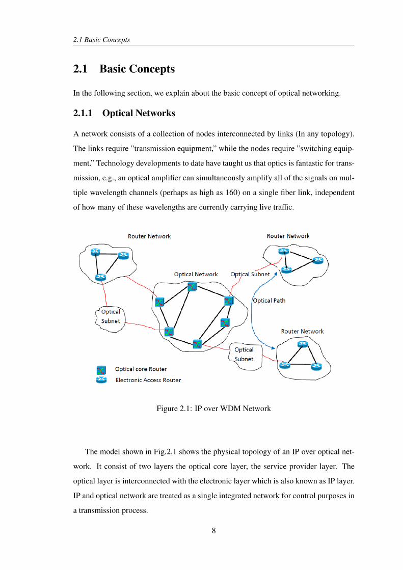
Figure 2.1: IP over WDM Network
The model shown in Fig.2.1 shows the physical topology of an IP over optical net-
work. It consist of two layers the optical core layer, the service provider layer. The
optical layer is interconnected with the electronic layer which is also known as IP layer.
IP and optical network are treated as a single integrated network for control purposes in
a transmission process.
8
2.1 Basic Concepts
• Services are not specifically defined at IP-optical interface, but folded into end-
to-end MPLS services.
• Routers may control end-to-end path using traffic engineering (TE)-extended rout-
ing protocols deployed in IP and optical networks.
An optical network is not necessarily all-optical, the transmission is certainly opti-
cal, but the switching could be optical, or electrical, or hybrid. Also, an optical is not
necessarily packet-switched. It could switch circuits, or sub-wavelength-granularity
bandwidth pipes, or ”bursts,” where a burst is a collection of packets. Based on the
various optical technologies, the most-prevalent deployment of optical networks to-
day consists of optical-electrical-optical (OEO) switches (also called opaque switches),
with each input operating at OC-192 (approx. 10 Gbps) rate. However, inside the OEO
switch, each input channel can be de-multiplexed into STS-1 timeslots” and the switch
can perform switching at STS-1 granularity. Thus, a network operator can support a
variety of connection requests ranging in bandwidth from STS-1 to OC-192.
2.1.2 Wavelength Division Multiplexing (WDM)
Wavelength-division multiplexing (WDM) is a technique that can exploit the huge opto-
electronic bandwidth mismatch by requiring that each end user’s equipment operate
only at electronic rate, but multiple WDM channels from different end-users may be
multiplexed on the same fiber [11]. Thus, by allowing multiple WDM channels to co-
exist on a single fiber, one can tap into the huge fiber bandwidth, with the corresponding
challenges being the design and development of appropriate network architectures, pro-
tocols, and algorithms. End-users in a fiber-based WDM backbone network may com-
municate with one another via optical (WDM) channels, which are referred to as light-
paths. A light-path may span multiple fiber links, e.g., to provide a ”circuit-switched”
interconnection between two nodes which may have a heavy traffic flow between them
and which may be located ”far” from each other in the physical fiber network topology.
Each intermediate node in the light-path essentially provides an optical bypass facility
to support the light-path.
9
2.1 Basic Concepts
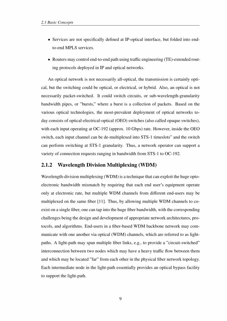
Figure 2.2: WDM Transmission System
A wavelength division multiplexing schemeFig.2.2 usually comprised of following
system
1. Transmitter: The optical transmitter converts the electrical signal into optical
form and launches the resulting optical signal into the optical fiber. It consists
of an optical source, a modulator, and a channel coupler. Semiconductor lasers
or light-emitting diodes are used as optical sources because of their compatibility
with the optical-fiber communication channel. The optical signal is generated by
modulating the optical carrier wave.
2. Communication Channel: The role of a communication channel is to transport the
optical signal from transmitter to receiver without distorting it. Most light-wave
systems use optical fibers as the communication channel because silica fibers
can transmit light with losses as small as 0.2 dB/km [12]. Even then, optical
power reduces to only 1 percent after 100 km. For this reason, fiber losses remain
an important design issue and determine the repeater or amplifier spacing of a
long-haul light-wave system. Another important design issue is fiber dispersion,
which leads to broadening of individual optical pulses with propagation. If optical
pulses spread significantly outside their allocated bit slot, the transmitted signal
is severely degraded. Eventually, it becomes impossible to recover the original
signal with high accuracy. The problem is most severe in the case of multimode
fibers, since pulses spread rapidly because of different speeds associated with dif-
10
2.1 Basic Concepts
ferent fiber modes. It is for this reason that most optical communication systems
use single-mode fibers. Material dispersion (related to the frequency dependence
of the refractive index) still leads to pulse broadening, but it is small enough to
be acceptable for most applications and can be reduced further by controlling the
spectral width of the optical source.
3. Receiver: An optical receiver converts the optical signal received at the output
end of the optical fiber back into the original electrical signal. It consists of a
coupler, a photo-detector, and a demodulator. The coupler focuses the received
optical signal onto the photo-detector. Semiconductor photodiodes are used as
photo-detectors.
2.1.3 Dense Wavelength Division Multiplexing (DWDM)
Light has an information-carrying capacity 10,000 times greater than the highest radio
frequencies. It is seen that due to transmission of signal in an optical medium, signal
strength will be reduced, known as attenuation loss. Further developments in fiber
optics are closely tied to the use of the specific regions on the optical spectrum where
optical attenuation is low. These regions, called windows, lie between areas of high
absorption. The earliest systems were developed to operate around 850 nm, the first
window in silica-based optical fiber. A second window (S band), at 1310 nm, soon
proved to be superior because of its lower attenuation, followed by a third window (C
band) at 1550 nm with an even lower optical loss. Today, a fourth window (L band)
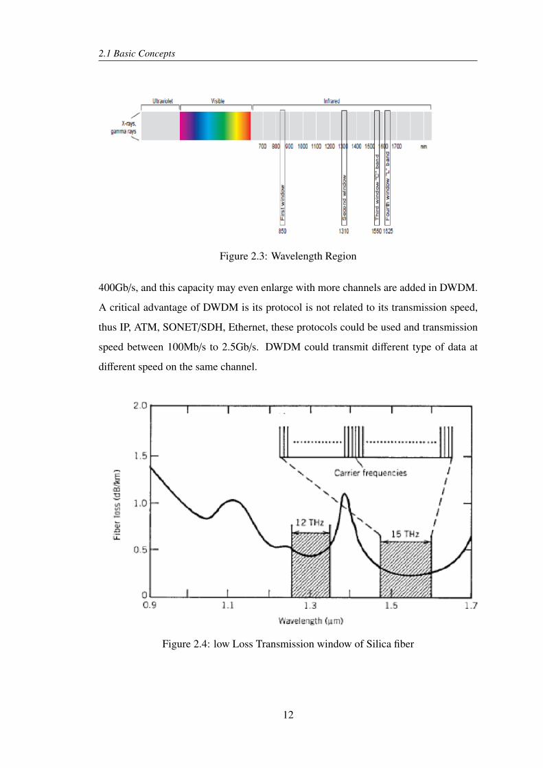
near 1625 nm is under development and early deployment (shown in Fig.2.3).
Dense Wavelength Division Multiplexing (DWDM) is an important technology in
nowadays fiber optic network. DWDM and CWDM both use WDM technology to ar-
range several fiber optic lights to transmit simultaneously via the same single fiber optic
cable, but DWDM carry more fiber channel compared with CWDM (Coarse Wave-
length Division Multiplexing). DWDM is usually used on fiber optic backbones and
long distance data transmission and DWDM system has higher demand of fiber ampli-
fiers. Due to DWDM technology, a single optical fiber capacity nowadays could reach
11
2.1 Basic Concepts
Figure 2.3: Wavelength Region
400Gb/s, and this capacity may even enlarge with more channels are added in DWDM.
A critical advantage of DWDM is its protocol is not related to its transmission speed,
thus IP, ATM, SONET/SDH, Ethernet, these protocols could be used and transmission
speed between 100Mb/s to 2.5Gb/s. DWDM could transmit different type of data at
different speed on the same channel.
Figure 2.4: low Loss Transmission window of Silica fiber
12
2.2 Multi Protocol Label Switching (MPLS)
Fig.2.4 shows the low-loss transmission windows of optical fibers centered near
1.3 and 1.55?m. Of the two types of WDM (broadband and narrow band), broadband
WDM uses the 1300nm and 1550nm wavelength for full duplex transmission, that is,
if a signal is sent in one direction by 1300nm, it can be sent back by 1550nm via the
same optical fiber. Narrowband WDM, which is the DWDM we are talking here, is
the multiplexing of 4, 8, 16, 32 or more wavelengths in the range of 1530nm to 1610nm
range with a very narrow separation between the wavelengths. Nowadays, the word
WDM often refers to the DWDM systems.
2.2 Multi Protocol Label Switching (MPLS)
MPLS has its roots in several IP packet switching technologies under development in
the early and mid 1990s. In 1996 the IETF started to pull the threads together, and in
1997 the MPLS Working Group was formed to standardize protocols and approaches
for MPLS. IP packet switching is the process of forwarding data packets within the
network, based on some tag or identifier associated with each packet. In some senses,
traditional IP routing is a form of packet switching, each packet carries a destination IP
address that can be used to determine the next hop in the path toward the destination
by performing a look-up in the routing table. However, IP routing has concerns about
speed and scalability, and these led to investigations of other ways to switch the data
packets. Added to these issues was the desire to facilitate additional services such as
traffic aggregation and traffic engineering.
2.2.1 MPLS Layering Structure
Multiprotocol Label Switching (MPLS) is a data forwarding technology for use in
packet networks. It is a switching technology high-performance telecommunications
networks which directs and carries data from one network node to the next with the
help of labels. It is a connection-oriented data carrying mechanism that traverses pack-
ets from source to destination node across networks. It has the feature of encompassing
packets in the presence different network protocols.
In IP routing, packets undergo analysis at each hop, followed by forwarding decision
using network header analysis and then lookup in routing table. In an MPLS network,
13
2.2 Multi Protocol Label Switching (MPLS)
packets carrying data are assigned with labels on each node and the forwarding decision
is totally based on these label headers. This is different from the conventional routing
mechanism. Packet header is analyzed only once while they enter the MPLS cloud
from then the forwarding decision is ’label-based’ that ensures fast packet transmission
between local-local and local-remote nodes.
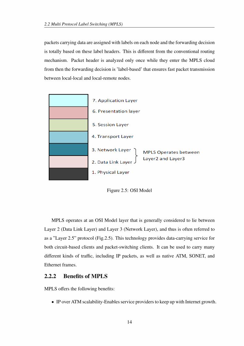
Figure 2.5: OSI Model
MPLS operates at an OSI Model layer that is generally considered to lie between
Layer 2 (Data Link Layer) and Layer 3 (Network Layer), and thus is often referred to
as a ”Layer 2.5” protocol (Fig.2.5). This technology provides data-carrying service for
both circuit-based clients and packet-switching clients. It can be used to carry many
different kinds of traffic, including IP packets, as well as native ATM, SONET, and
Ethernet frames.
2.2.2 Benefits of MPLS
MPLS offers the following benefits:
• IP over ATM scalability-Enables service providers to keep up with Internet growth.
14
2.2 Multi Protocol Label Switching (MPLS)
• IP services over ATM-Brings Layer 2 benefits to Layer 3, such as traffic engi-
neering capability.
• Standards-Supports multivendor solutions.
• Architectural flexibility-Offers choice of ATM or router technology, or a mix of
both
2.2.3 Notation and Definitions
In this section we describe the notations and definitions used in our work.
• LSR - Label Switching Router-It operates at the edge of the MPLS network.
• LSP - Within the MPLS domain, a path is setup for a given packet to travel based
on an FEC, which is called a label switching path (LSP).
• LER - Label Edge Router-It support multiple ports connected to different net-
works and forward to the MPLS network after establishing LSP. It plays a im-
portant role in the assignment and removal of labels as traffic enters or exits an
MPLS networks.
• LIB - Each LSR build a table to specify how packets must be forwarded. This
table is called a label information base (LIB).
• FEC - Forward Equivalent Class is a group of IP packets. Each LSR build a
table to specify how a packet must be forwarded. This table is called a Label
Information Base (LIB).
2.2.4 MPLS Labels
1. MPLS header: The 32-bit MPLS header contains the following fields.
• The label field (20-bits) carries the actual value of the MPLS label.
• The Class of Service (CoS) field (3-bits) can affect the queuing and discard
algorithms applied to the packet as it is transmitted through the network.
Since the CoS field has 3 bits, therefore 8 distinct service classes can be
possible.
15
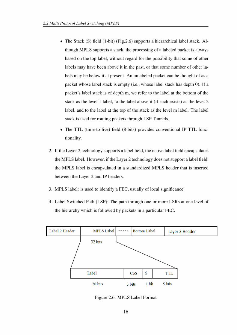
2.2 Multi Protocol Label Switching (MPLS)
• The Stack (S) field (1-bit) (Fig.2.6) supports a hierarchical label stack. Al-
though MPLS supports a stack, the processing of a labeled packet is always
based on the top label, without regard for the possibility that some of other
labels may have been above it in the past, or that some number of other la-
bels may be below it at present. An unlabeled packet can be thought of as a
packet whose label stack is empty (i.e., whose label stack has depth 0). If a
packet’s label stack is of depth m, we refer to the label at the bottom of the
stack as the level 1 label, to the label above it (if such exists) as the level 2
label, and to the label at the top of the stack as the level m label. The label
stack is used for routing packets through LSP Tunnels.
• The TTL (time-to-live) field (8-bits) provides conventional IP TTL func-
tionality.
2. If the Layer 2 technology supports a label field, the native label field encapsulates
the MPLS label. However, if the Layer 2 technology does not support a label field,
the MPLS label is encapsulated in a standardized MPLS header that is inserted
between the Layer 2 and IP headers.
3. MPLS label: is used to identify a FEC, usually of local significance.
4. Label Switched Path (LSP): The path through one or more LSRs at one level of
the hierarchy which is followed by packets in a particular FEC.
Figure 2.6: MPLS Label Format
16
2.3 Generalised Multi Protocol Label Switching (GMPLS)
In MPLS, the assignment of a particular packet to a particular FEC is done just once,
as the packet enters the network. The FEC to which the packet is assigned is encoded
as a label. When a packet is forwarded to its next hop, the label is sent along with it.
At subsequent hops, there is no further analysis of the packet’s network layer header.
Rather, the label is used as an index into a table which specifies the next hop, and a new
label. The old label is replaced with the new label, and the packet is forwarded to its
next hop.
2.2.5 MPLS operations
The implementation of MPLS for data forwarding involves the following four steps:
1. MPLS label assignment (label creation and Distribution).
2. MPLS LDP (between LSRs/ELSRs).
3. MPLS label distribution (using a label distribution protocol).
4. MPLS label retention
MPLS operation typically involves adjacent LSR’s forming an LDP session, as-
signing local labels to destination prefixes and exchanging these labels over established
LDP sessions. Upon completion of label exchange between adjacent LSRs, the control
and data structures of MPLS, namely FIB, LIB, and LFIB, are populated, and the router
is ready to forward data plane information based on label values.
2.3 Generalised Multi Protocol Label Switching (GM-PLS)
Generalized Multi-Protocol Label Switching (GMPLS) is developed by the IETF for
transport network control planes [6]. GMPLS is a new protocol suite that uses ad-
vanced network signaling and routing mechanisms to automate set up for end-to-end
connections for all types of network traffic. GMPLS is becoming increasingly widely
17
2.3 Generalised Multi Protocol Label Switching (GMPLS)
used as a control plane in optical circuit switched networks due to its capability to al-
low a seamless integration of a multitude of technologies, especially circuit switched
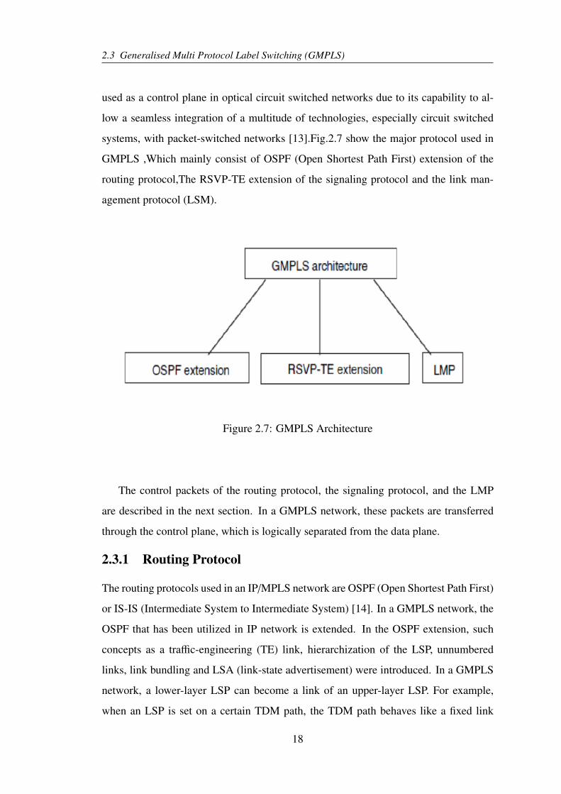
systems, with packet-switched networks [13].Fig.2.7 show the major protocol used in
GMPLS ,Which mainly consist of OSPF (Open Shortest Path First) extension of the
routing protocol,The RSVP-TE extension of the signaling protocol and the link man-
agement protocol (LSM).
Figure 2.7: GMPLS Architecture
The control packets of the routing protocol, the signaling protocol, and the LMP
are described in the next section. In a GMPLS network, these packets are transferred
through the control plane, which is logically separated from the data plane.
2.3.1 Routing Protocol
The routing protocols used in an IP/MPLS network are OSPF (Open Shortest Path First)
or IS-IS (Intermediate System to Intermediate System) [14]. In a GMPLS network, the
OSPF that has been utilized in IP network is extended. In the OSPF extension, such
concepts as a traffic-engineering (TE) link, hierarchization of the LSP, unnumbered
links, link bundling and LSA (link-state advertisement) were introduced. In a GMPLS
network, a lower-layer LSP can become a link of an upper-layer LSP. For example,
when an LSP is set on a certain TDM path, the TDM path behaves like a fixed link
18
2.3 Generalised Multi Protocol Label Switching (GMPLS)
that has been there permanently for a long time. When the lower-layer LSP is set, the
originating node of the LSP, when viewed from the upper layer, is advertised within the
network as an upper-layer link. This LSP is called a TE link. When PSC-LSP is set
up, the route is selected according to the topology that is constructed by TE links. In
general, in the topology of a GMPLS network, a physical link, such as an optical fiber, is
also called a TE link. The interface of a link in an MPLS network is generally assigned
an IP address. According to this IP address, it is possible to identify the link inside
the network. However, in a GMPLS network, because it is possible to accommodate
more than 100 wavelengths per one optical fiber, the number of required IP addresses
becomes huge if an IP address is assigned to each interface of these wavelengths. In
GMPLS, to identify the link a link identifier (link ID) that is assigned to the interface of
the link has been introduced. It is possible to identify the link inside the network from
a combination of the router ID and the link ID.
2.3.2 Signaling Protocol
The signaling protocol is a protocol that sets up the LSP and manages the setup status
of the LSP. RSVP-TE signaling of an MPLS network is extended for use in a GMPLS
network. Setting up the LSP means to switch the packets according to the label conver-
sion table, in which correspondence between the label of the input link and the label of
the output link of the node on the route of the LSP has been set, by assigning the label
of the link through which the LSP passes. In MPLS, label assignment executes just to
set up the LSP route, but not to assign the bandwidth or network resource. In GMPLS,
the label corresponds to the time slot in the TDM layer, to the wavelength in the λ-layer,
and to the fiber in the fiber layer. Therefore, assigning the label in a GMPLS network
means to assign the bandwidth or network resource in layers other than the packet layer.
This point that label assignment means to assign the bandwidth or network resource is
a characteristic of the extended RSVP-TE for GMPLS.
2.3.3 Link Management Protocol
To manage the link between neighboring nodes, a Link Management Protocol (LMP)
has been introduced as a GMPLS protocol [15]. LMP has four functions: Control-
19

2.3 Generalised Multi Protocol Label Switching (GMPLS)
channel management, Link-property correlation, Connectivity certification, Failure man-
agement. Control-channel management and link-property correlation are indispensable
functions of LMP, and connectivity certification and failure management are optional
functions.
20

System Design
Bandwidth Model
Delay Model
Q-Factor Model
Chapter 3
System Design
As defined in previous chapter WDM technology, allow a single optical fiber to transmit
multiple optical carrier signals by using different wavelength to carry different carrier
of signal. DWDM increases this capacity of transmission of signal in optical fiber
communication. This technique multiplex signals of different wavelengths and provides
data capacity in hundreds of gigabits per second over thousands of kilometers in a single
mode fiber with more security. Similarly MPLS, GMPLS protocol make it easy to
transmit signal in different layers of communication system.
In this Chapter, first section discuses about the system model. Second section gives
the overview control plane protocol and TCM algorithm, third section deals with the
design of different mathematical model, Fourth section explain about path selection
algorithm.
3.1 System Model
A System model gives the layout of interconnections of the various elements like links,
nodes, etc. of a network system. Nodes in a network are represented by the coordinate
where the location of a node is given by point in a coordinate system. In a network, a
node is a connection point, either a redistribution point or an end point for data trans-
missions. Link in a network is a connection through optical fiber link between two
nodes. In a system link between too nodes is represented by the line joining between
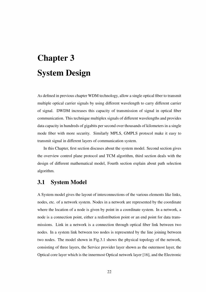
two nodes. The model shown in Fig.3.1 shows the physical topology of the network,
consisting of three layers, the Service provider layer shown as the outermost layer, the
Optical core layer which is the innermost Optical network layer [16], and the Electronic
22
3.1 System Model
intermediate layer or also known as IP layer.
Figure 3.1: physical Topology
This is an abstraction of the combined electro-optical network which allows us to
focus on that portion of the network where our innovation applies, i.e. the combined
electro-optical network. The optical layer provides point-to-point connectivity between
routers in the form of fixed bandwidth circuits, which is termed as light-paths. The col-
lection of light-paths therefore defines the topology of the virtual network interconnect-
ing electronics/IP Routers. In IP layer the IP routers are responsible for all the non-local
management functions such as management of optical resources, configuration and ca-
pacity management, addressing, routing, topology discovery, traffic engineering, and
restoration etc. The IP router communicates with the TCM (Traffic Control Manager)
of service provider network and provides the information about the status of the optical
layer.
Ideally the service provider layer will include elements of the access network such
as the PON (Passive Optical Network) related elements and other devices/equipment
located at the premises/home. However for this invention such details are not necessary.
23
3.2 Control Plane Protocol and TCM Algorithm
We assume that the service provider has access to General Purpose Routers and also
optical components in the core optical network. Such an assumption is reasonable,
given the fact that the prices of optical switching equipment have fallen by orders of
magnitude till the point that they are being used in the premises of large corporations in
order to interconnect buildings etc. Thus it is reasonable to assume, as we have done,
that the service provider has information about the GPRs and the optical equipment
within its domain of control.
The service provider layer controls all the traffic corresponding to both IP and op-
tical layers. All the routers shown in the figure are controlled by the service provider
(SP). The SP maintains a traffic matrix in a Traffic Control Manager (TCM) for all the
connected general purpose routers, i.e. all the Electronic Gateway Routers (EGR), Elec-
tronic Access Routers (EAR) and Optical Access Routers (OAR) within its domain of
control.
The Traffic Control Manager (TCM) maintains the network as well as PLI con-
straints such as Capacity, delay, and Q-factor matrices for all the GPRs in the network,
belonging to all the layers. In the following sections we outline our algorithms that
carry out the computations necessary for the decisions that lead to provisioning/de-
provisioning of data-paths.
3.2 Control Plane Protocol and TCM Algorithm
If i and j are connected GPRs within the network, then the Traffic Control Matrix el-
ement T (i, j) provides useful information regarding the flow of traffic between i and
j. The Table 3.1 shows all control protocols used for GPRs pair (i, j) and shows how
our algorithm provides a solution in areas where other approaches do not. We assume
that the information maintained by T (i, j) includes capacity, end-end-delay, and overall
Q-Factor between the GPRs, as well as the total quantum of committed traffic between
the two routers. An admission control algorithm operating within the control of the ser-
vice provider allows traffic flows to operate between the routers after making sure that
capacity is available. There are various techniques for achieving this in the IP routers,
such as RSVP, Diff-Serv and Bandwidth Broker. Any of these techniques are acceptable
24
3.3 Problem Formulation
Table 3.1: Control Plane Protocoli,j OCR OAR EGR EAR
OCR G+A G+A Not Possible Not PossibleOAR G+A G+A M+G+A M+G+AEGR Not Possible M+G+A M+A M-TE+AEAR Not Possible M+G+A M-TE+A M+A
for the algorithms presented herein.
Notations: G =GMPLS, M =MPLS, M-TE =MPLS-TE, A =Our Algorithm From
Table 3.1, we see that our algorithm applies to all possible combinations of all types of
routers.
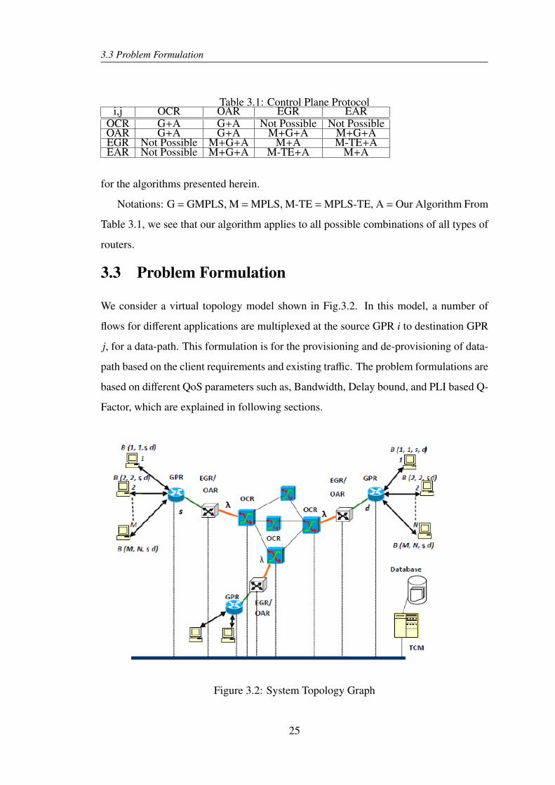
3.3 Problem Formulation
We consider a virtual topology model shown in Fig.3.2. In this model, a number of
flows for different applications are multiplexed at the source GPR i to destination GPR
j, for a data-path. This formulation is for the provisioning and de-provisioning of data-
path based on the client requirements and existing traffic. The problem formulations are
based on different QoS parameters such as, Bandwidth, Delay bound, and PLI based Q-
Factor, which are explained in following sections.
Figure 3.2: System Topology Graph
25
3.3 Problem Formulation
3.3.1 Bandwidth Model
Assume every DWDM client end point is attached to at most one GPR. Suppose a flow
for client m and n with light-path from source s to destination d has bandwidth/traffic
requirement BR(m, n, s, d). The aggregated traffic flow for them is defined as:
TAggrt(m, n, s, d) =∑m,n
BR(m, n, s, d) (3.1)
As per the network condition, for every edge GPR, a free available capacity matrix,
B(m, n, s, d) has been considered, where s and d are the source and destination edge
GPRs for a light-path.
Assume the physical layer constants are dispersion, spectral width of light and link
length. If DS (i, j) is the dispersion of the fiber at the operating wavelength with units
seconds per nanometer per kilometer, and L(i, j) is the length of fiber link pair (i, j) in
kilometers, the bandwidth matrix can be mentioned [17] as follows:
B(i, j) =δ
DS (i, j) ×√
L(i, j)(3.2)
where, δ represents the pulse broadening factor should typically be less than 10
parcent of a bit’s time slot for which the polarization mode dispersion (PMD) can be
tolerated [10] and D(i, j) = L(i, j) =∞, when there is no link from i to j. The bandwidth
matrix for a light-path will be:
B(m, n, s, d) = Min {B(i, j)} ,∀(i, j) ∈ P(s, d) (3.3)
Where,p(s, d) is the computed light-path for source (s) to destination (d) containing
a group of links.The capacity metrics B(m, n, s, d) calculation is derived from a single
link to a group of links in a Light-path.
3.3.2 Delay model
Next, we estimating the delay requirement for the clients that support guaranteed ser-
vice in terms of end-to-end delay bound. In Fig.3.2, suppose the delay requirement of
26
3.3 Problem Formulation
flow for (m, n) client pair from source s and destination d is D(m, n, s, d). The maximum
acceptable delay between s and d is as follows:
DAcceptMax (m, n, s, d) = Min {D(m, n, s, d)} ,∀(m, n) (3.4)
Where,m = 1, 2 · · ·M and n = 1, 2, · · ·Nand M and N are the total number OVPN
clients attached to source s and d respectively. As per the network condition if D(i, j)
is the link pair delay, then the end-to-end delay is the sum of link delays suffered by a
connection at all routers along with the light-path p(s, d) and given as:
DBoundMax =
∑(i, j)∈P(s,d)
D(i, j) (3.5)
Where, according to [18],
D(i, j) = a + bλ2i,k + cλ−2
i,k (3.6)
Where a,b and c are fiber material dependant constants also known as fit parameter,
λi,k is the wavelength at ith node and its kth light-path. Here we have taken aluminium
oxide and Silicon oxide as the fiber material for simulation work.
3.3.3 Q-Factor Model
We defined the link cost as the ratio of bandwidth and delay, which is termed as Q-
Factor and will be represented as below.
QF(i, j) =B(i, j)D(i, j)
(3.7)
Then for a complete light-path p(s, d) of source (s) and destination (d), the Q-Factor
will be:
QF(m, n, s, d) = Min {Q(i, j)} ,∀(i, j) ∈ P(s, d) (3.8)
Assume QFr(m, n, s, d) is the Q-Factor required from OPVN client m and n for
source (s) and destination (d) pair. It can be defined as follows:
QFr(m, n, s, d) =TAggrt(m, n, s, d)
DAcceptMax (m, n, s, d)
(3.9)
27
3.4 TCM Mechanism for Light-Path Provisioning
3.4 TCM Mechanism for Light-Path Provisioning
The TCM algorithm for the provisioning of new Light-Path based on the equations 1
to 9. The edge GPR aggregates the bandwidth, acceptable delay and Q-Factor require-
ment of the flows as mentioned in equation 3.1, 3.4 and 3.9. This aggregated bandwidth
and acceptable delay will be compared with the estimated bandwidth and delay bound
mentioned in equation 3.3 and 3.5 respectively. Also both estimated Q-Factor and re-
quired Q-Factor mentioned in equation 8 and 9 will be compared in order find a best
suitable network. The comparison takes decision, whether to provision a network for
the requested services.
3.4.1 Light-Path provisioning based on only Bandwidth and Delay
The provisioning of Light-Path for any of the following conditions.
DAcceptMax (m, n, s, d) ≥ DBound
Max (m, n, s, d) (3.10)
TAggrt(m, n, s, d) < B(m, n, s, d) (3.11)
3.4.2 Light-Path provisioning based on Q-Factor
The provisioning of Light-Path occurs for any of the following conditions.
QFr(m, n, s, d) ≤ QF(m, n, s, d) (3.12)
3.4.3 De- provisioning based on Q-Factor based on Required Q-Factor
The de-provisioning of light path occurs for the following condition.
QFr(m, n, s, d) << QF(m, n, s, d) (3.13)
28
3.5 Algorithm for Light-Path Selection
3.5 Algorithm for Light-Path Selection3.5.1 Algorithm for light-path selection based on Bandwidth and
Delay
• STEP1: Calculate Delay for each link using the delay equation (3.6).
• STEP2: To find the overall Delay bound find the sum of delay of the links belong
to the possible light-path using equation (3.5).
• STEP3: Compare the acceptable delay value and bound delay in STEP2 and
check the condition in equation (3.10).
• STEP4: Check whether aggregate traffic is less than bandwidth or not using equa-
tion (3.11).
• STEP5: If condition in STEP3 and STEP4 satisfy, provision OVPN light-path,
which is the selected light-path.
• STEP6: STOP
29
3.5 Algorithm for Light-Path Selection
3.5.2 Algorithm for light-path selection based on Q-Factor
• STEP1: Calculate the Q-Factor for each link for the Q-Factor equation (3.7).
• STEP2: Then calculate the overall light-path Q-Factor for source s and destina-
tion d, which is the minimum value of links Q-Factor using equation (3.8).
• STEP3: Required Q-Factor for OVPN client m and n for source s and destination
d using equation (3.9).
• STEP4: Check for condition in equation (3.12), If satisfy provisioning of light-
path occur based on Q-Factor, else repeat STEP1, STEP2, STEP3 for other light-
path.
• STEP5: If the condition in equation (3.13) is satisfy, de-provisioning occur and
repeat above steps to compute a light-path.
30
3.6 Fiber Material Selection Mechanism for QoS Enhancement
3.6 Fiber Material Selection Mechanism for QoS En-hancement
The fiber material which provides minimum delay during route computation that will
be considered to be used in fiber network back bone. The following is the flow chart
Fig.3.3 for the above mechanism.
Figure 3.3: Fiber material selection Flow-Chat
The selection mechanism show how to select fiber material based on the minimum
delay.Delay play a major role in data transmission technology.If we are able to select a
Light-Path before sending any data with minimum delay, then it is advantageous for the
client.
31
Simulation and ResultsNetwork Model
Selection based on Bandwidth
Selection based on Delay Q-Factor
Comparison Results
Chapter 4
Simulation and Results
This chapter discusses the simulation of light-path selection mechanism for the client
based on Bandwidth, Delay and Q-Factor requirement as describe in the earlier chapter.
Here we have considered three scenarios of how to obtain the best suitable light-path
depending on the above parameters. Also we simulate Path selection technique based
on delay for different fiber material to provide best light-path for the client.
4.1 Network Model
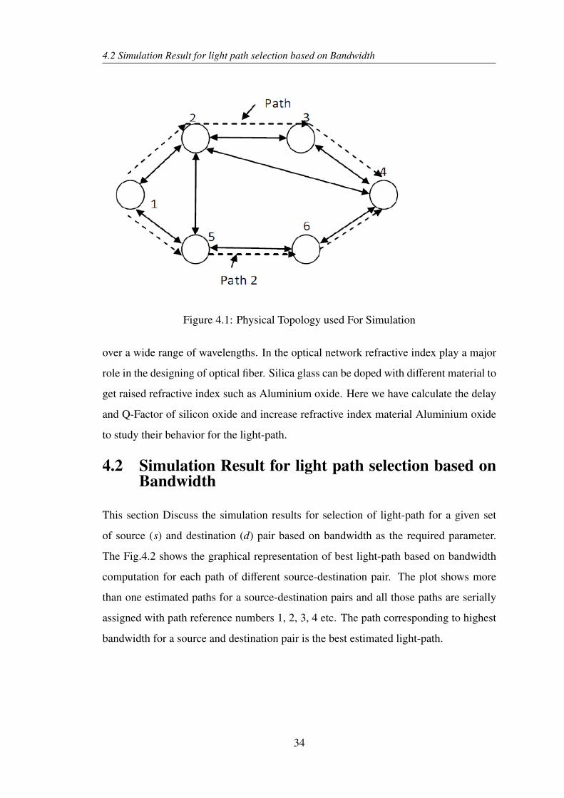
We have considered Fig.4.1 for the simulation, The Fig.4.1 shows the basic network
topology with 6 nodes. Here we computed three pair of source and destination nodes
(1, 4), (5, 3), and (1, 6) and their possible paths to choose the best path based on client
requirement. The light-path selection mechanism considers quality parameters such as
bandwidth, delay and Q-Factor for the finding of best suitable path.
In our simulation, we have considered three scenarios of how to obtain the best
suitable light-path, such as:
1. By considering bandwidth as the only quality requirement.
2. By considering Delay as the only quality requirement.
3. By considering both in terms of Q-Factor.
In this work we have taken silica glass as the fiber material and also doped material
of silica wit increase refractive index. Silica exhibits fairly good optical transmission
33
4.2 Simulation Result for light path selection based on Bandwidth
Figure 4.1: Physical Topology used For Simulation
over a wide range of wavelengths. In the optical network refractive index play a major
role in the designing of optical fiber. Silica glass can be doped with different material to
get raised refractive index such as Aluminium oxide. Here we have calculate the delay
and Q-Factor of silicon oxide and increase refractive index material Aluminium oxide
to study their behavior for the light-path.
4.2 Simulation Result for light path selection based onBandwidth
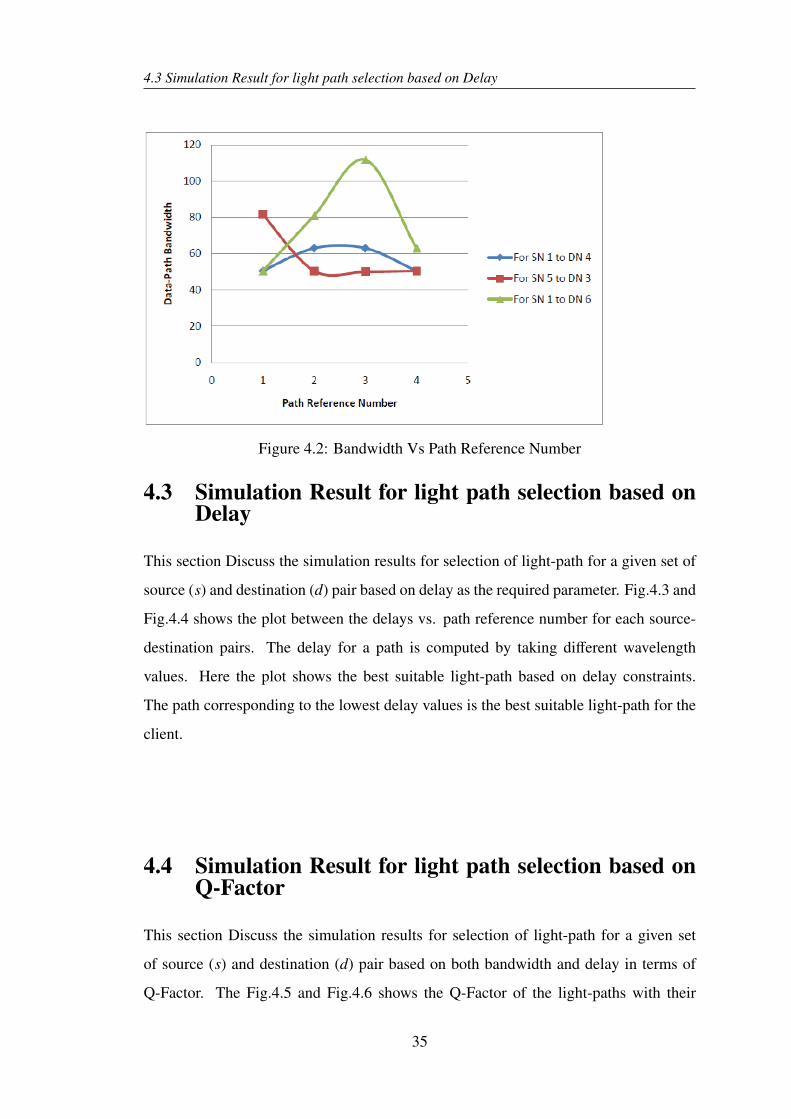
This section Discuss the simulation results for selection of light-path for a given set
of source (s) and destination (d) pair based on bandwidth as the required parameter.
The Fig.4.2 shows the graphical representation of best light-path based on bandwidth
computation for each path of different source-destination pair. The plot shows more
than one estimated paths for a source-destination pairs and all those paths are serially
assigned with path reference numbers 1, 2, 3, 4 etc. The path corresponding to highest
bandwidth for a source and destination pair is the best estimated light-path.
34
4.3 Simulation Result for light path selection based on Delay
Figure 4.2: Bandwidth Vs Path Reference Number
4.3 Simulation Result for light path selection based onDelay
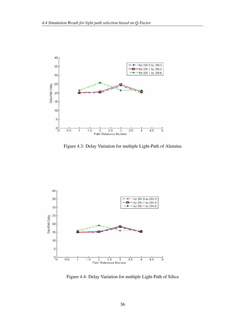
This section Discuss the simulation results for selection of light-path for a given set of
source (s) and destination (d) pair based on delay as the required parameter. Fig.4.3 and
Fig.4.4 shows the plot between the delays vs. path reference number for each source-
destination pairs. The delay for a path is computed by taking different wavelength
values. Here the plot shows the best suitable light-path based on delay constraints.
The path corresponding to the lowest delay values is the best suitable light-path for the
client.
4.4 Simulation Result for light path selection based onQ-Factor
This section Discuss the simulation results for selection of light-path for a given set
of source (s) and destination (d) pair based on both bandwidth and delay in terms of
Q-Factor. The Fig.4.5 and Fig.4.6 shows the Q-Factor of the light-paths with their
35
4.4 Simulation Result for light path selection based on Q-Factor
Figure 4.3: Delay Variation for multiple Light-Path of Alumina
Figure 4.4: Delay Variation for multiple Light-Path of Silica
36
4.4 Simulation Result for light path selection based on Q-Factor
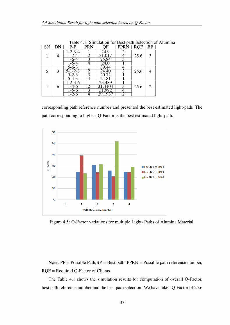
Table 4.1: Simulation for Best path Selection of AluminaSN DN P-P PRN QF PPRN RQF BP
1 41-2-3-4 1 24.9 2
25.6 31-2-4 2 31.017 41-6-4 3 25.84 31-5-4 4 24.0 1
5 35-6-3 1 39.44 4
25.6 45-1-2-3 2 24.40 25-2-3 3 20.72 15-4-3 4 24.81 1
1 61-2-3-6 1 23.489 1
25.6 21-4-6 2 31.4104 31-5-6 3 31.992 41-2-6 4 29.1937 2
corresponding path reference number and presented the best estimated light-path. The
path corresponding to highest Q-Factor is the best estimated light-path.
Figure 4.5: Q-Factor variations for multiple Light- Paths of Alumina Material
Note: PP = Possible Path,BP = Best path, PPRN = Possible path reference number,
RQF = Required Q-Factor of Clients
The Table 4.1 shows the simulation results for computation of overall Q-Factor,
best path reference number and the best path selection. We have taken Q-Factor of 25.6
37
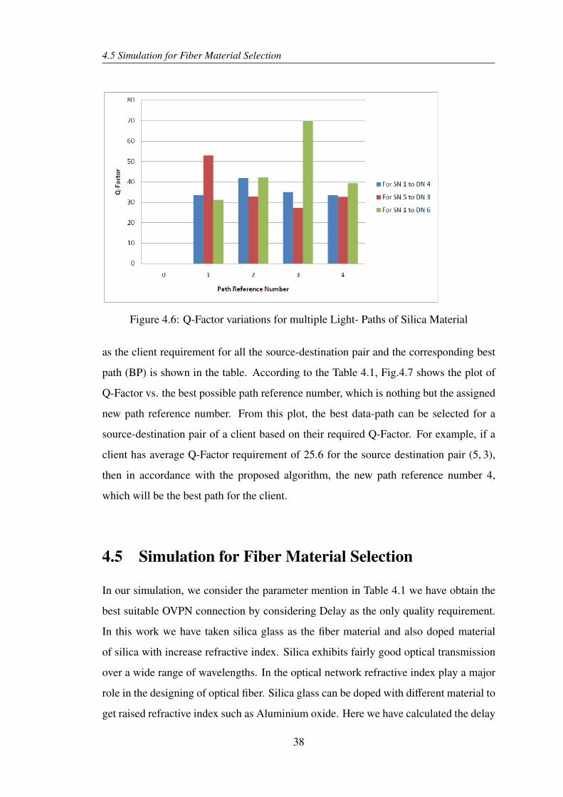
4.5 Simulation for Fiber Material Selection
Figure 4.6: Q-Factor variations for multiple Light- Paths of Silica Material
as the client requirement for all the source-destination pair and the corresponding best
path (BP) is shown in the table. According to the Table 4.1, Fig.4.7 shows the plot of
Q-Factor vs. the best possible path reference number, which is nothing but the assigned
new path reference number. From this plot, the best data-path can be selected for a
source-destination pair of a client based on their required Q-Factor. For example, if a
client has average Q-Factor requirement of 25.6 for the source destination pair (5, 3),
then in accordance with the proposed algorithm, the new path reference number 4,
which will be the best path for the client.
4.5 Simulation for Fiber Material Selection
In our simulation, we consider the parameter mention in Table 4.1 we have obtain the
best suitable OVPN connection by considering Delay as the only quality requirement.
In this work we have taken silica glass as the fiber material and also doped material
of silica with increase refractive index. Silica exhibits fairly good optical transmission
over a wide range of wavelengths. In the optical network refractive index play a major
role in the designing of optical fiber. Silica glass can be doped with different material to
get raised refractive index such as Aluminium oxide. Here we have calculated the delay
38
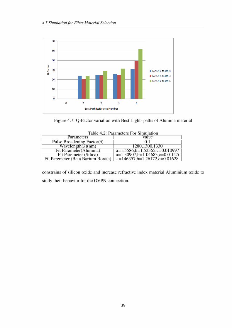
4.5 Simulation for Fiber Material Selection
Figure 4.7: Q-Factor variation with Best Light- paths of Alumina material
Table 4.2: Parameters For SimulationParameters Value
Pulse Broadening Factor(δ) 0.1Wavelength(λ)(nm) 1280,1300,1330
Fit Parameter(Alumina) a=1.5586,b=1.52365,c=0.010997Fit Paremeter (Silica) a=1.30907,b=1.04683,c=0.01025
Fit Paremeter (Beta Barium Borate) a=146357,b=1.26172,c=0.01628
constrains of silicon oxide and increase refractive index material Aluminium oxide to
study their behavior for the OVPN connection.
39
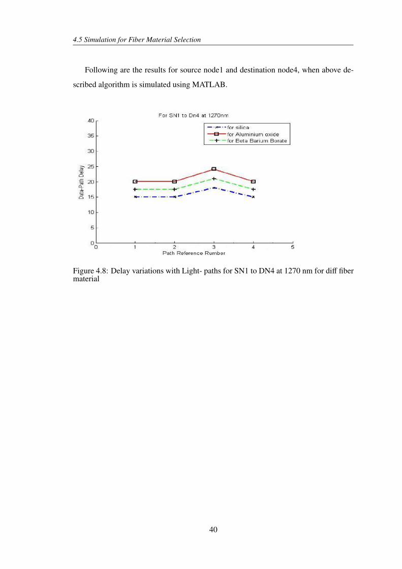
4.5 Simulation for Fiber Material Selection
Following are the results for source node1 and destination node4, when above de-
scribed algorithm is simulated using MATLAB.
Figure 4.8: Delay variations with Light- paths for SN1 to DN4 at 1270 nm for diff fibermaterial
40
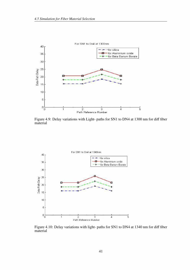
4.5 Simulation for Fiber Material Selection
Figure 4.9: Delay variations with Light- paths for SN1 to DN4 at 1300 nm for diff fibermaterial
Figure 4.10: Delay variations with light- paths for SN1 to DN4 at 1340 nm for diff fibermaterial
41
4.5 Simulation for Fiber Material Selection
Following are the results for source node1 and destination node6, when above de-
scribed algorithm is simulated using MATLAB.
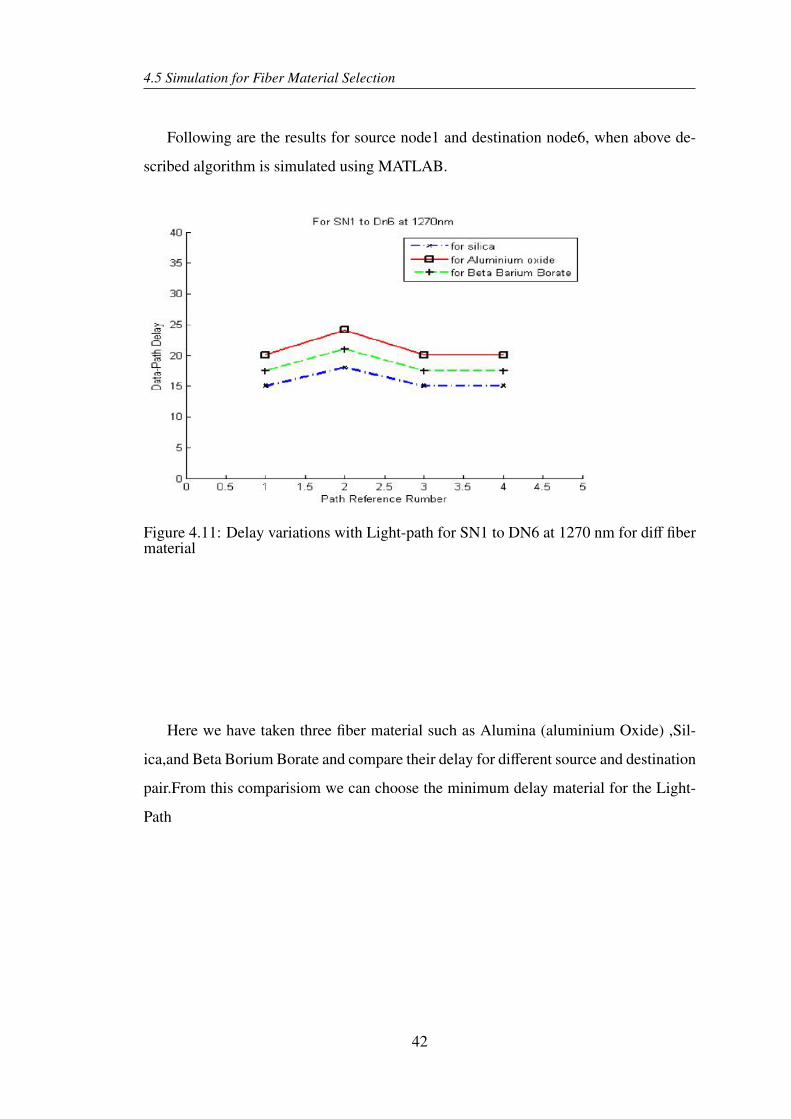
Figure 4.11: Delay variations with Light-path for SN1 to DN6 at 1270 nm for diff fibermaterial
Here we have taken three fiber material such as Alumina (aluminium Oxide) ,Sil-
ica,and Beta Borium Borate and compare their delay for different source and destination
pair.From this comparisiom we can choose the minimum delay material for the Light-
Path
42

4.5 Simulation for Fiber Material Selection
Figure 4.12: Delay variations with Light- paths for SN1 to DN6 at 1300 nm for difffiber material
Figure 4.13: Delay variations with Light- paths for SN1 to DN6 at 1340 nm for difffiber material
43

Conclusion and Future Work
Concluions
Future Work
Chapter 5
Conclusion and Future Work
This chapter presents the conclusion of the thesis and describing future directions. Sec-
tion 5.1 summarizes the conclusion of the thesis. Section 5.2 highlights the directions
for the future work.
5.1 Conclusions
In this thesis, We have presented an algorithm that determines the condition when to
provision light-paths or remove existing ones in a GMPLS network. Here we have
considered three scenarios to provision a best suitable light-path as per the client re-
quirements of bandwidth and delay. If the light-path provisioned by bandwidth and
delay, the corresponding light-paths might not be suitable for one of the requirements.
In case of light-path provisioning based on Q-Factor, the corresponding path will be
well suited to both the requirements, which we say a guaranteed service. What makes
the algorithm unique is the fact that it performs traffic engineering at TCM for both IP
and Optical layer by allocating light-path to the end clients. This mechanism performs
a global optimization based upon three factors such as aggregated flow, delay and Q-
Factor requirements. The outcome of the global optimization is a new allocation rate
and decision criteria to drop or add light-paths for an existing or new clients.
5.2 Future Works
The proposed method provides a Light-Path selection mechanism, which flexible to
the service provider as well as the client.Based on the client requirement our method
provide the suitable path by considering the required parameters. This method can be
45

5.2 Future Works
further enhanced by adding a concept of Generalised Multi Protocol Label Switching
(GMPLS), which is applied in Optical Virtual private Network (OVPN). Also this is
method can be improved in data transmission of Storage Area Network (SAN).
46
Bibliography
[1] H. Beyranvand and J. Salehi, “Multiservice provisioning and quality of service
guarantee in wdm optical code switched gmpls core networks,” Lightwave Tech-
nology, Journal of, vol. 27, pp. 1754 –1762, june15, 2009.
[2] C. Saradhi and S. Subramaniam, “Physical layer impairment aware routing (pliar)
in wdm optical networks: issues and challenges,” Communications Surveys Tuto-
rials, IEEE, vol. 11, pp. 109 –130, quarter 2009.
[3] L. Georgiadis, R. Guerin, V. Peris, and R. Rajan, “Efficient support of delay
and rate guarantees in an internet,” SIGCOMM Comput. Commun. Rev., vol. 26,
pp. 106–116, August 1996.
[4] J. Glasmann, M. Czermin, and A. Riedl, “Estimation of token bucket parame-
ters for videoconferencing systems in corporate networks,” SoftCOM, vol. 2000,
pp. 10–14, 2000.
[5] S. Blake, D. Black, M. Carlson, E. Davies, Z. Wang, and W. Weiss, “An architec-
ture for differentiated service,” 1998.
[6] N. Zhang and H. Bao, “Research on wdm optical transport network with gm-
pls technology,” in Computer Science and Information Technology, 2009. ICCSIT
2009. 2nd IEEE International Conference on, pp. 323 –326, aug. 2009.
[7] L. Zhang, S. Deering, D. Estrin, S. Shenker, and D. Zappala, “Rsvp: a new re-
source reservation protocol,” Communications Magazine, IEEE, vol. 40, pp. 116
–127, may 2002.
47
BIBLIOGRAPHY BIBLIOGRAPHY
[8] Z.-L. Zhang, Z. Duan, L. Gao, and Y. T. Hou, “Decoupling qos control from core
routers: a novel bandwidth broker architecture for scalable support of guaranteed
services,” SIGCOMM Comput. Commun. Rev., vol. 30, pp. 71–83, August 2000.
[9] G. Bernstein, B. Rajagopalan, and D. Saha, Optical Network Control: Architec-
ture, Protocols, and Standards. Boston, MA, USA: Addison-Wesley Longman
Publishing Co., Inc., 2003.
[10] Q. Liu, M. Kok, N. Ghani, V. Muthalaly, and M. Wang, “Hierarchical inter-domain
routing in optical dwdm networks,” in INFOCOM 2006. 25th IEEE International
Conference on Computer Communications. Proceedings, pp. 1 –5, april 2006.
[11] B. Mukherjee, optical WDM Networks. Optical Network Series, Springer.
[12] G. Agrawal, Fiber-Optic Communications Systems. Wiley, 3rd ed., 2002.
[13] O. Komolafe and J. Sventek, “Rsvp performance evaluation using multi-objective
evolutionary optimisation,” in INFOCOM 2005. 24th Annual Joint Conference of
the IEEE Computer and Communications Societies. Proceedings IEEE, vol. 4,
pp. 2447 – 2457 vol. 4, march 2005.
[14] E. O. Naoaki Yamanaka, Kohei shiomoto, “Gmpls technologies broadband back-
bone networks and systems,” Taylor and Francis 4th ed, 2006.
[15] J. Lang, “Link management protocol (lmp),” ietf draft, http://www.ietf.org/
internet-drafts/draft-ietf-ccamp-lmp-10.txt, Oct 2003.
[16] J. Strand, A. Chiu, and R. Tkach, “Issues for routing in the optical layer,” Com-
munications Magazine, IEEE, vol. 39, pp. 81 –87, feb 2001.
[17] Y. Huang, J. Heritage, and B. Mukherjee, “Connection provisioning with trans-
mission impairment consideration in optical wdm networks with high-speed chan-
nels,” Lightwave Technology, Journal of, vol. 23, pp. 982 – 993, march 2005.
[18] Y. Miyajima, M. Ohnishi, and Y. Negishi, “Chromatic dispersion measurement
over a 120 km dispersion-shifted single-mode fibre in the 1.5 micrometer wave-
length region,” Electronics Letters, vol. 22, pp. 1185 –1186, 23 1986.
48
Dissemination of Work
1. S. K. Das, S. K. Naik and S. K. Patra ` Centralized Data-path Control Mechanism
for DWDM/GMPLS Network ´ , International Conference on Signal Acquisition
and Processing (ICSAP 2011), February 26-28, 2011, Singapore.
2. S. K. Das, S. K. Naik and S. K. Patra ` Fiber Material Dependent QoS Analysis
and OVPN Connection Setup Over WDM/DWDM Network ´ , TENCON-2011,
November 21-24, 2011, Bali, Indonesia.(Submitted).
3. S. K. Das, S. K. Naik and S. K. Patra ` A GMPLS based QoS framework for
Optical Virtual Private Network ´ ,IEEE/OSA, Journal Of Light wave Technology,
May 2011.(In Press).
49