Q-Rap HelpQ-Rap is licensed under the GNU General Public License version 3

www.QRap.org.za

Table of Contents1)Introduction......................................................................................................................................42)Getting Started................................................................................................................................5

2.1)Installing Ubuntu......................................................................................................................52.2)Install the base software Q-Rap depends on...........................................................................5

2.2.1) Install Synaptic Package Manager..................................................................................52.2.2)Configure Additional QGIS Repositories...........................................................................52.2.3)Install All Required Software and Libraries.......................................................................5

3)Installing Q-Rap on Ubuntu.............................................................................................................73.1)Compiling from source.............................................................................................................73.2)Creating the Database.............................................................................................................73.3)Loading the demo database (Optional)....................................................................................83.4)Setting up Q-Rap.....................................................................................................................8

3.4.1)Activate the Q-Rap-plugin................................................................................................83.4.2)Set up a map in QGIS......................................................................................................83.4.3)Make the Q-Rap spatial information visible......................................................................93.4.4)Setting up the Q-Rap-database........................................................................................9

3.4.4.1)Set up a Technology ................................................................................................93.4.4.2)Import a few antenna pattern files...........................................................................103.4.4.3)Create a Mobile installation.....................................................................................103.4.4.4)Generate default entries..........................................................................................113.4.4.5)Default Entries per Technology...............................................................................133.4.4.6)Set-up Plot defaults.................................................................................................133.4.4.7)Set-up Colours for the Maps...................................................................................143.4.4.8)Add DEM and Clutter raster files.............................................................................15

4)A Few First Examples....................................................................................................................164.1)Loading Digital Elevation Model.............................................................................................164.2)Creating a site........................................................................................................................174.3)Do a Coverage Prediction......................................................................................................174.4)Perform a link analysis...........................................................................................................19

5)Description of User Interface Functionalities..................................................................................205.1)Place Site button....................................................................................................................205.2)Place Site dialogue box..........................................................................................................20

5.2.1) Move Site to … button ..................................................................................................205.2.2) Just a Site button...........................................................................................................215.2.3)Add Default Installation button........................................................................................215.2.4)Edit Installation button....................................................................................................215.2.5)Cancel button.................................................................................................................21

5.3)Select a Site button................................................................................................................215.3.1) Update button................................................................................................................215.3.2) Edit Installation button...................................................................................................21

5.4)Delete a Site button...............................................................................................................215.5)Link Analysis button...............................................................................................................215.6)Confirm Link Analysis dialogue box (4.4)..............................................................................215.7)Link Analysis Display.............................................................................................................22

5.7.1)Export to PDF button......................................................................................................225.7.2)Align Antennae button....................................................................................................225.7.3)Save button....................................................................................................................225.7.4)Ok button........................................................................................................................225.7.5)Cancel button.................................................................................................................22

5.8)Select Link button..................................................................................................................23

5.9)Delete Link button..................................................................................................................235.10)Perform Area Prediction button............................................................................................235.11)Confirm Prediction Information dialog box............................................................................23

5.11.1)Radio Installation Selection Table................................................................................235.11.2)Prediction Type.............................................................................................................235.11.3)Output File Name.........................................................................................................235.11.4)Output Directory...........................................................................................................245.11.5)Mobile Radio Used.......................................................................................................245.11.6)Minimum Required Received Signal Level (dBm?).......................................................245.11.7)Required Carrier to Co-channel Interference Ratio (dB)...............................................245.11.8)Required Carrier to Adjacent-channel Interference Ratio (dB)......................................245.11.9)Required energy per Bit to Noise Ratio (dB).................................................................245.11.10)Down-link or Up-link Radio button..............................................................................255.11.11)Output Units...............................................................................................................255.11.12)Fade Margin (dB)........................................................................................................255.11.13)Noise Level (dBm)......................................................................................................255.11.14)Required Signal to Noise Ratio (dB)...........................................................................255.11.15)k-Factor for Servers....................................................................................................255.11.16)k-Factor for Interference.............................................................................................255.11.17)Predict selected area (with radius included) radio button............................................255.11.18)Plot Resolution (meter)...............................................................................................265.11.19)Minimum Angular Resolution (degrees)......................................................................26

5.12)Multi-link identification button...............................................................................................265.13)Multi-Link Identification Dialogue Box..................................................................................26

5.13.1)Site Selection Table......................................................................................................265.13.2)Technology...................................................................................................................265.13.3) Project.........................................................................................................................265.13.4) Maximum Path Loss (dB)............................................................................................275.13.5) Maximum Distance (km)..............................................................................................275.13.6)Minimum Clearance (%)...............................................................................................275.13.7)k-Factor........................................................................................................................27

5.14)Link Optimisation.................................................................................................................285.14.1)Prerequisites................................................................................................................28

5.14.1.1)Costs.....................................................................................................................285.14.1.2)Existing Mast Heights............................................................................................285.14.1.3)Receiver Capabilities............................................................................................28

5.14.2)Optimisation Button and Dialogue Box.........................................................................285.14.3)Optimisation Settings....................................................................................................29

5.14.3.1)Technology...........................................................................................................295.14.3.2)Project...................................................................................................................29

5.14.4)Site Information............................................................................................................305.14.5)Optimisation Parameters..............................................................................................30

5.14.5.1)Height Range For No Existing Mast......................................................................305.14.5.2)Minimum Links Requirement Per Site...................................................................30

5.14.6)Antennas, Cables, Combiners and Splitters.................................................................315.14.7)Link Feasibility Factors.................................................................................................31

5.14.7.1)Maximum Path Loss.............................................................................................315.14.7.2)Maximum Distance...............................................................................................315.14.7.3)Minimum Signal Strength......................................................................................325.14.7.4)Minimum Links Requirement Per Site...................................................................325.14.7.5)Minimum Clearance..............................................................................................325.14.7.6)k-Factor.................................................................................................................325.14.7.7)Transmitter Power.................................................................................................325.14.7.8)Receiver Sensitivity...............................................................................................325.14.7.9)Data-Rate.............................................................................................................32

5.14.8)Output Directory and Buttons.......................................................................................325.14.8.1)Output PDF Settings and Directory.......................................................................335.14.8.2)OK Button.............................................................................................................33

5.14.8.3)Cancel Button.......................................................................................................335.15)Spectral Interference Calculation button..............................................................................335.16)Spectral Interference Analysis Dialog Box ..........................................................................34

5.16.1)Radio Installation Selection Table................................................................................345.16.2)Receiver Station: .........................................................................................................345.16.3)k-Factor........................................................................................................................345.16.4)Frequency Resolution (kHz).........................................................................................34

5.17)Preferences Button..............................................................................................................355.17.1)Q-Rap Preferences dialogue box.................................................................................36

5.17.1.1)System Units.........................................................................................................365.18)Database Interface...............................................................................................................36

6)Parameters....................................................................................................................................367)Analysis Functionalities.................................................................................................................378)Design and Planning Assistance Functionalities............................................................................37

1) IntroductionQ-Rap is an Open Source Radio Planning software package, which can be used by cellular

operator, radio amateurs, people installing any form radio based technology, to do radio coverage analysis and link planning.

The core origin of this package was developed specifically for the South African Police Services’ Radio Technical Services which paid for the initial development and specified that the software be release as Open Source to enable the continued development and maintenance thereof. This original project was done via/by Business Enterprises at the University of Pretoria (BE@UP) and executed mainly by Magdaleen Ballot from the Department for Electictrical, Electronic and Computer Engineering at the University of Pretoria. The copyright belongs to the University of Pretoria. The core propagation prediction algorithms originates from the GISRAP tool developed by the Meraka Institute, then Mikomtek at the CSIR. The copyright these classes re-used from the GISRAP code hence belongs to the Meraka Institute. Meraka also paid for the further development of a multi-link identification tool, while the Department of Science and Technology sponsored the development of the Spectral Analysis tool for the Square Kilometer Array project. The South African Police Services(SAPS), the University of Pretoria and the Meraka Institute has all agreed to release the code under the General Public License.

The core properties of this package are:• It is based on an Open Source Geographic Information System (QGIS), which enables easy

integration with all GIS functionalities.• It has an fairly flexible open database structure, that allows easy changes and translations. It is

based on Open Source PostgreSQL.• The use of Open Source Postgis enables a number of spatial queries on the data.• The use of the open source package GDAL allows the use of almost any Digital Elevation Model

format.• Most package choices (e.g. open source Qt for interface development) were made to allow it to be

Operating System independent.• The database structure and design choices were made to allow for various and multiple wireless

technologies.• Data that is visible can be filtered based on location, technology, project and other criteria.• The core propagation prediction model is based on free-space loss calculations and the multiple

knife-edge diffraction losses done according to the Deygout method. It includes addition losses for rounded hills.

• The effective earth model is used. The k-Factor, i.e. the ratio of the real earth radius to the effective earth radius, reflects the gradient of the refractiveness of the lower earth, and hence the curvature of the path of the radio waves. This model originates from the Mikomtek, CSIR, now the Meraka Institute.

• Easy to use, particularly when compared to other free mobile planning tools.• Amble use of tool-tips to ease use.

The following functionalities are currently included:• Link Analysis including Fresnel Zone clearance.• Coverage prediction that calculates the received signal strength at all points for one or many radio

installations,• Primary Server calculations that indicates the actual 'cell' area of each radio installation,• Number of server calculations, with which coverage overlap can be determined. • Interference calculations based on frequency assignments in the database.• Loading of small area of the Digital Terrain Data• Spectral Interference analysis for inter-system interference analysis• Automatic tool for the identification of visible links among a set of sites.

For help on QGIS functionalities please refer to the QGIS manual.

2) Getting Started

2.1) Installing UbuntuThe instructions on how to obtain Ubuntu and install it, can be found on the following pages

http://www.ubuntu.com/getubuntu/downloadhttp://www.ubuntu.com/

The CD/DVD image could also be downloaded from:http://ubuntu.saix.net/ubuntu-releases/precise/

orftp://ftp.wa.co.za/pub/ubuntu/releases/precise/

2.2) Install the base software Q-Rap depends on.

2.2.1) Install Synaptic Package ManagerThe team knows/prefers the Synaptic Package Manager; since Ubuntu Software Centre is the

default package manager front end for newer Ubuntu releases, Synaptic needs to be installed first.Use the Ubuntu Software Centre to search for and install Synaptic. After installation of Synaptic is done, close the Software Centre and open Synaptic.

2.2.2)Configure Additional QGIS Repositories"Repositories" refer to location where software packages and source code are stored on the

Internet. In order to compile Q-Rap, the QGIS 2.0 or later is required. The QGIS additional repository locations needs to be registered with Synaptic in order to gain access to them. In Synaptic, follow the steps shown below:

• Select the Settings->Repositories menu• Select the “Other Software” tab, (the second tab) on the "Software Sources" window that opens.• Click the "Add..." button, and then enter the APT line shown below in the dialog window that

opens, confirming with the "Enter" key:

deb http://qgis.org/debian precise main

• Also add the source or development repository below, using the same procedure as the previous step:

deb-src http://qgis.org/debian precise main

• Ensure that the tick-boxes next to the newly added repositories are checked.• Close the "Software Sources" window when done.• Back on the main Synaptic window, click the "Reload" button on the top tool bar; this will force

Synaptic to refresh its repository data.• If an GPG error occurs for the QGIS repositories added stating that signatures could not be

verified, one needs to add the public key: Do this by entering the command given below in separate command line console (note that the key value to enter should be the same as reported by the error message):

sudo apt-key adv --keyserver keyserver.ubuntu.com --recv-keys EBB1B7ED997D3880

• After adding the public key, click the Synaptic "Reload" button again, the error message should not appear again.

For more information about QGIS packages an public keys, see http://www.qgis.org.

2.2.3)Install All Required Software and Libraries• In Synaptic Package Manager, search and install all listed packages.• Ensure that you use the Synaptic "Search" function, not the default "Quick Search".

• Ensure that the repository data is up to date by clicking the "Reload" button in the Synaptic tool bar menu before installing new packages.

• Some packages listed below may already be installed on the system, but might be out of date. By selecting "Mark All Upgrades" in the Synaptic tool bar menu, these packages will be shown with a green "up arrow" icon. This signifies that the package will be upgraded when applying changes. Packages that are out of date and not marked for upgrade is shown with a gray exclamation icon. Individual packages can be marked for upgrade by right clicking and selecting "Mark for Upgrade"

• Once all packages are marked for install or upgrade, click on the "Apply" button in the Synaptic tool bar menu. Your Internet link speed will determine the length of the coffee break you can take at this point.

Using the Search (not Quick Search) you must find and mark the following packages for installation:• qgis• libqgis-dev (make sure all older versions of qgis and the development files are removed

completely)• libgdal1-dev (once again ensure that you have only one version of gdal installed)• libgeos++-dev• g++• cpp• gpp• cmake• subversion• flex• bison• libpoco-dev• qt4-designer• qt4-dev-tools• libqt4-core• libqt4-dev• libqt4-sql-psql• libqwt5-qt4-dev• libpqxx-dev• postgresql• postgresql-server-dev-9.1 (or latest)• postgis• postgresql-9.1-postgis (or latest)• libeigen3-dev

The following packages are optional:• postgresql-doc• tora (database interface tool)• xiphos

Now, might also be a good time to Mark All Upgrades to ensure that you have the latest software installed. Downloading and installation might take a while, so take a break once you hit the Apply-button. Go to the gym, home, lunch, meeting …

3) Installing Q-Rap on Ubuntu

3.1) Compiling from sourceThe first releases of Q-Rap will need to be compiled from source. To obtain the source you must enter the following on the command line: (search for "Terminal" at the Dash Home on the top-left corner of your screen to find and open a command line terminal)

svn checkout http://svn.code.sf.net/p/qrap/code/ qrap

this points Subversion to the server that currently contains Q-Rap. Once it has been downloaded (enough time for a cuppa coffee) you can compile Q-Rap. The source code will be provided in the directory ‘/qrap/’. On the command line, go to the /qrap/ directory. You can use

• pwd to determine your present working directory• cd .. to go one directory up and • ls –l to view the content of the current directory and• cd qrap to go to the qrap directory

In this directory runcmake ./

to configure the makefile. Take note of any dependencies that might still not be resolved and download these packages. Then to compile the package run:

make(Time to refill the coffee mug.)and to install run

sudo make installyou will be asked for the password of the main user. Q-Rap should now exist but, alas, you will first need a database.

3.2) Creating the DatabaseChange the password of the postgres user

sudo passwd postgreschange it to postqrap to make life simple at firstStill in the command line, log-on as user postgres

su postgresGo to the /qrap/DataBase/ directory by typing

cd DataBase Run the script CreateDB.sh.

./CreateDB.sh

If you have problems with the scripts you can try the following:• Confirm the permissions of the qrap directory and DataBase and Prediction subdirectories:

o Using the file browser right click each (sub)directory. Select Permissions. Make sure that all users have create, delete, read and write permissions to all the files.

o If this does not work enterexitgoto the /qrap/ base directoryand thensudo postgres chown <subdirectory>/ for the DataBase and Prediction subdirectories respectively.

Try the above again.• Make CreateDB.sh executable:

o In the file browser right click on the file, go to Permissions and tick the “Allow executing file as program” tick-box.

• Make sure you are using the correct PostGIS script directory

o Open the CreateDB.sh file for editing, and change the PostGISDir variable to the directory on your machine containing postgis.sql file. A easy way to determine this is by looking at the location of the “installed files” in Synaptic for your particular version of postgres-v.v-postgis.

• Make sure tDataBase/makefile is referencing the correct gdal version. o Removing the 1.7.0 at the end of -lgdal1.7.0 resulting in -lgdal should work for gdal

versions 1.9 and later. • Another problem might be that the default port 5432 is not applicable to / available on your

machine, then you need to change the file qrap/DataBase/settings.xml, and change the port to for example 5433.

3.3) Loading the demo database (Optional)

If you just quickly want to get an feel for what this tool can do, this is really recommended. However the demo database does not exist yet:We must write a script that will load all the data including the height data that you will be able to use.

3.4) Setting up Q-Rap

3.4.1)Activate the Q-Rap pluginTo get most feedback it is best to run QGIS from the command line. Simply type:

qgis

Activate the Q-Rap plug-in:On the tool-bar of QGIS, select command Plugins, and Plugin Manager and select at least Q-Rap and SPIT, but you may want to try out some of the other plug-ins as well.On closing the QGIS Plugin Manager, the Login Dialog box will appear:

All you need to do is fill in the password, which should be postqrap, unless you changed the CreateDB.sh script. The port setting might also be different: e.g. 5433 and the host might simply be referred to as localhost.

The Q-Rap tool-bar should now appear on the QGIS interface. It might be necessary to rearrange the Tool-bars a bit to make it visible.

3.4.2)Set up a map in QGISYou can refer to the QGIS help for more information on how to go about adding layers. To provide some form of visual reference on the map you can add a vector layer by clicking on the Add a Vector

Layer icon, , and finding a normal shape file to add. Some examples are available in /qrap/Data/ Shapefiles/.

3.4.3)Make the Q-Rap spatial information visible

Click on the Add a PostGIS Layer, , icon. Add a New database and complete the following information and click OK.

Connect to the database and Add the selected Site and Link information to be displayed.On the QGIS tool-bar Save Project. This will allow you to avoid all this setting up next time you start. You can additional layers to the postgis-layer of the qrap-database using the SPIT tool (look for the blue elephant). It might be for example be a good idea to add the provincial boundaries. These boundaries could later be used as a why to filter for different sites.

3.4.4)Setting up the Q-Rap-databaseIn this section we will only briefly go through all the steps that are required to get going using Primary GSM as an example technology. For a complete discussion of each step you will have to refer to the latter sections of the manual.

The first step is to open up the database interface: Click on the Q-Rap Database Interface icon, .

3.4.4.1) Set up a Technology Select the Supporting Tables tab, and the Technology Form View to complete the following and Commit it to the database:

3.4.4.2) Import a few antenna pattern filesQ-Rap imports any antenna file that is in “planet” format. Some antenna suppliers make files in this format available. A few samples files are available in /qrap/Data/AntennaFiles/.

On the toolbar of the database user interface select File,Import,

Antenna Files.Select the Technology that will be served with these antennas patterns. Browse for and select the antennas you would like to import. Select OK.

Alternatively, the Antenna Device and Antenna Pattern Form Views could be used to enter your first antenna pattern in the database.

3.4.4.3) Create a Mobile installationThe mobile installations are used to represent the subscribers units when doing coverage predictions.

3.4.4.4) Generate default entriesThe first entry of a table (with primary key 0) will generally be used to set the default entries into any

given table. Select the Preference icon, , or select

Edit, Preferences

on the Q-Rap Database Interface tool-bar. Select

RAPDefaults

and select the Edit Defaults radio button.Now you can proceed to enter all the tables you would like to with default entries in each field. It might be a particularly good idea to at least provide defaults for the Radio Installation table with sensible default entries. First you need to add the default site:

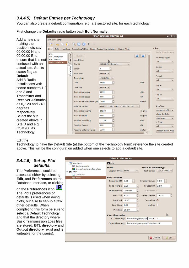
3.4.4.5) Default Entries per TechnologyYou can also create a default configuration, e.g. a 3 sectored site, for each technology:

First change the Defaults radio button back Edit Normally.

Add a new site, making the position lets say 00:00:00 N and 00:00:00 E to ensure that it is not confused with an actual site. Set its status flag as DefaultAdd 3 Radio Installations with sector numbers 1,2 and 3 and Transmitter and Receiver Azimuths as 0, 120 and 240 degrees respectively. Select the site created above in SiteID and e.g. GSM900 as Technology.

Edit the Technology to have the Default Site (at the bottom of the Technology form) reference the site created above. This will be the configuration added when one selects to add a default site.

3.4.4.6) Set-up Plot defaults.

The Preferences could be accessed either by selecting Edit, and Preferences on the Database Interface, or clicking

on the Preferences icon, . The Plots preferences or defaults is used when doing plots, but also to set-up a few other defaults. When completing this form be sure to select a Default Technology and that the directory where Basic Transmission Loss files are stored, BTL directory and Output directory exist and is writeable for the user(s).

Now might also be a good idea to confirm that your preferences for the input formats are selected:

3.4.4.7) Set-up Colours for the Maps

Defaults colours for the different kind of maps could be set-up using Preferences Dialogue box. First enter the number of bands and the minimum and maximum values you expect, then click on Classify which will render default starting values, that can be edited by clicking on each entry.

3.4.4.8) Add DEM and Clutter raster files

To “import” the raster files select File, Import and then Raster Files on Q-Rap Database Interface.

Here we will only present an example. More detailed information is available in a later section.

First create a new File Set to which the files could be added. In this example we will add the SRTM data that is available from http://srtm.csi.cgiar.org/ or you can directly go to http://srtm.csi.cgiar.org/SELECTION/inputCoord.asp . ArcInfoASCII (or GeoTiff) format can be used. The gdal libraries (http://www.gdal.org/) is used to load these files, so most files could be loaded selecting the File Format “GDALFILE”. The files could be loaded as either DEM (Digital Elevation Model) for the local ground height data or Clutter for land cover type data.

Next one needs to add the references to these files in the database. Select the newly created File Set, and Browse for, select and Open the files. To Import the files might take a while … you are probably in need of a break.

When the files are completely installed the Files to be imported list, will be clear.

It is important to Set the File Set Usage Order (Raster File Operation on the left hand of the dialog box). Add the newly created FileSet to the list for the DEM FileType.

4) A Few First Examples

4.1) Loading Digital Elevation Model

Click on the Perform a Prediction icon, , and with the mouse's left button select an area for which you would like view the Digital Elevation Model data, ending the selection with a right button click. If the area does not include any site, a information or warning message will appear. Upon closing this message box, The Prediction Dialogue box will appear. The Digital Elevation Model is the last option

available under Prediction. Click on Do. When the height data has been loaded the Done can be used to close the Dialogue Box. An example of such a DEM is shown below.

4.2) Creating a site.

Click on the Place a Site icon, , point the cursor to the location where you would like to place a site and click on the left mouse button. First you are informed that to obtain the height data at the point might take a while. Click on OK and wait for the dialog box to appear. To add a set of installations like those edited in paragraph 3.4.4.4 click on Add Default Installation.

4.3) Do a Coverage Prediction

Once again by clicking on the Perform a Prediction icon, , and selecting an area that includes all the sites for which you would like to include in the prediction, ending with a right click will bring the Prediction dialog box up. Click Do to start the prediction. This might take a while. The Radius determine the maximum distance from the site for which the prediction will be done.

Many prediction options are available. They will be discussed in later sections. Two examples are a Coverage plot that indicates the receivable signal strength at different locations and the other a Primary Server plot that indicates which radio installation will provide the strongest signal.

4.4) Perform a link analysisCreate another site, in a similar manner described in 4.2. Note that both sites need to have a radio installation attached.

Click on the Link Analysis icon, , then on the first site, and then on the second. The link request dialogue box should appear. After selecting the radio installation between which you would like to do the link analysis click on Ok. Below is the resultant Link Analysis. Saving the link stores it in the database. Clicking on the Align Antennae will result in changing the radio installations in the database to point to one another. It also analyses the link again.

5) Description of User Interface Functionalities

5.1) Place Site buttonThis button is a way to create a site via the QGIS user interface.

• Click on the button, • move the mouse cross-point to the location where you would like to place the site. • Left click again. • A information dialogue box will appear requesting

you to wait a while, close it by clicking on Ok.• Wait until the Site Dialogue box appears:

5.2) Place Site dialogue box

5.2.1) Move Site to … button This buttons allows one to again use the QGIS user interface to move the site position:• Click on the button, • move the cross-hair mouse position to the the

position where you would like to place the site,• Left click.

• The coordinates of the new position will appear in the dialogue box. The position shown will not move until one of the three accepting buttons are clicked:

5.2.2) Just a Site buttonIf you just want to add a site, but do not want to place any radio installation on the site, clicking on this button will store the site in the database and close the dialogue box.

5.2.3)Add Default Installation buttonClicking on this button will save the site and add copies of all the radio installations connected to the default site (3.4.4.5) of the current default technology as selected in Plot Preferences (3.4.4.6). It results in the dialogue box being closed.

5.2.4)Edit Installation buttonClicking on this button will save the site in the Database, close the dialogue box and take you to the Database User Interface where you will be able to edit, and commit (a) radio installation(s) that is connected to this site.

5.2.5)Cancel buttonThis button will close the dialogue box WITHOUT saving the site information in database.

5.3) Select a Site buttonTo edit a site click on this button. The same dialogue box as above will appear, and the functionalities will be exactly the same as in (5.1) except:

5.3.1) Update buttonThis will save any changes you made to the information in the dialogue box in the database can close the dialogue box.

5.3.2) Edit Installation buttonAfter closing the dialogue box clicking on this button will take you to the information of any existing radio installations on the site and allow you to edit it via the Database User Interface.

5.4) Delete a Site buttonClicking on this button will bring up a confirmation dialogue box. On clicking Delete, the site and any radio installation and or any other information linked to that site will be removed from the database.

5.5) Link Analysis buttonTo create a site-to-site radio link between two sites that already have radio installation installed:• Click on this button.• Move the mouse to the site that you would like to serve as transmitter.• Left click.• Move mouse to site that were the receiving radio installation will be.• Left click.The Link Analysis dialogue box (4.4)will appear.

5.6) Confirm Link Analysis dialogue box (4.4)• Use the radio buttons select the radio installation you would like to use for the transmitter and

receiver respectively.• The radio button on the bottom allows you to an analysis using the Tx radio installation as the actual

transmitter (Downlink) or the Rx radio installations transmitting part (Uplink).

• The Link Name may be any recognisable name and duplicates may occur.For help on the remaining parameters see Section 6.Click Ok and wait a bit. The Link Analysis Display will appear:

5.7) Link Analysis Display

5.7.1)Export to PDF buttonThis allows one to save the information of the link on a *.pdf file of your choice. It does not save it in the database.

5.7.2)Align Antennae buttonThis alters the radio installations involved to point to one another, which means the actual azimuth and tilt of the antennae will change to the recommended values. This change is save in the database. The link is however not saved in the database.

5.7.3)Save buttonClicking on this button will result in the Link being saved in the database. When an existing link was selected (5.8), this will result in the link being updated in the database.

5.7.4)Ok buttonTo close the display click on this button.

5.7.5)Cancel buttonThis button also make the Link Display button disappear.

5.8) Select Link buttonTo view the Link Analysis of a Link in the database, • click on this button, • move the mouse pointer to anywhere on the line representing the link. • Left click.The Confirm Link Analysis dialog box (5.6) will appear with the actual values of the link in the dialog box. You may now edit these values and press Ok, to view the Link Analysis Display (5.7). Pressing the Save button will now result in updating the link in the database.

5.9) Delete Link buttonTo delete a link from the database • click on this button, • move the mouse pointer to any point on the line representing the link. • Left click.A confirmation dialog box will appear. Press Ok to delete the link. The radio installations on either side of the link will also be removed from the database. (The sites with any other radio-installation on it will remain).

5.10) Perform Area Prediction buttonThis button enables one to perform any of a number of possible area analyses. These are described in detail in Section 7. To perform any of these analysis.• Left click on this button• Using the left mouse button mark a polygon on the QGIS user interface that includes all the sites

that you would like to include in the analysis. • End the selection with the right mouse button.The Confirm Prediction Information Dialog Box should appear.

5.11) Confirm Prediction Information dialogue boxThe Prediction Information that can be edited are:

5.11.1)Radio Installation Selection TableThis table contains a row for each Radio Installation in the selected area. • The tick boxes allow for these installations to be included(ticked) or excluded (unselected) in the

prediction analysis.• The only other entry that really makes sense to edit is the Radius. It is the maximum radius from the

site for which the prediction will be done. The default value supplied here originates from the setting in the Technology table (3.4.4.1)for the Technology of that site, if it was specified, otherwise the default value will be that supplied in the Plot Preferences (3.4.4.6).

The remaining columns are there to ease the identification of the Radio Installations.

5.11.2)Prediction TypeIn this combo box one can select the type of plot you would like to have generated. In Section (7) you will find a complete description of each of these options.

5.11.3)Output File NameThe default output filename corresponds to the Prediction Type or Plot Type. This could be changed to anything. At this stage the file extension needs to remain *.img.

5.11.4)Output DirectoryThis is actually more informational. This is the directory where the output file is saved. It can be altered under Plot Preferences (3.4.4.6). Make sure that the current user has write access to this directory.

5.11.5)Mobile Radio UsedThis is a selection from the Mobile table (3.4.4.3) entries. This is to represent any mobile, cellphone or handhold unit for which the coverage is to be planned.

5.11.6)Minimum Required Received Signal Level (dBm?)This determines the minimum level that will be displayed on the plot. Signal levels below this level will not be displayed as coverage at all (a value of -9999 is assigned, which will be transparent). The default value is determined by the values set in the Plot Preferences (3.4.4.6). More detail on how to chose this parameter will be found in Section 6

5.11.7)Required Carrier to Co-channel Interference Ratio (dB)This value will be used in the interference related plots as criteria when interference should be displayed. The default value is determined by the values set in the Plot Preferences (3.4.4.6). More detail on this parameter will be found in Section (6).

5.11.8)Required Carrier to Adjacent-channel Interference Ratio (dB)This value will be used in the interference related plots as criteria when interference should be displayed. The default value is determined by the values set in the Plot Preferences (3.4.4.6). More detail on this parameter will be found in Section (6).

5.11.9)Required energy per Bit to Noise Ratio (dB)This value will be of particular importance CDMA based systems. Currently it is not incorporated in any plot. The default value is determined by the values set in the Plot Preferences (3.4.4.6). More detail on this parameter will be found in Section (6).

5.11.10)Down-link or Up-link Radio buttonNormally when doing area predictions the prediction is done on the down-link, i.e. with the fixed installation or base station as the transmitter and the mobile unit as the receiver. It is however often useful to present the value that would be received by the base-station from a mobile transmitter at the point in the area. The default is determined by the values set in the Plot Preferences (3.4.4.6).

5.11.11)Output UnitsThis determines the units in which particularly the Coverage Plot will be presented. The default value is determined by the values set in the Plot Preferences (3.4.4.6). More detail on the meaning of different output units will be found in Section (6).

5.11.12)Fade Margin (dB)This represent a margin that is introduced to ensure that a certain percentage of the signal will be above the required level in a fading environment. Currently it is not incorporated in any plot. The default value is determined by the values set in the Plot Preferences (3.4.4.6). More detail on how to chose this parameter will be found in Section 6

5.11.13)Noise Level (dBm)This is the noise level or noise floor. The value is used in the signal to noise ratio plot. This level is determined by the bandwidth of the technology and the environmental noise sources present. More detail on how to chose this parameter will be found in Section 6 (In future versions this will be set as the power spectral density in e.g. dBm/Hz)

5.11.14)Required Signal to Noise Ratio (dB)The value is used in the signal to noise ratio plot. This value is mostly determined by the technology and the quality of the equipment. The default value is determined by the values set in the Plot Preferences (3.4.4.6). More detail on this parameter will be found in Section 6

5.11.15)k-Factor for ServersThis parameter is used in the effective earth model. It depends on the gradient of the refractiveness of air just above the surface of the earth. The value for servers will be used for the serving calculations in Coverage Plots and Interference-Plots. Values between 0.96 and 1.33 are typical. The smaller the value the more likely it is that hills and mountain will obstruct the wave. The default value is determined by the values set in the Plot Preferences (3.4.4.6). More detail on this parameter will be found in Section (6).

5.11.16)k-Factor for InterferenceThis parameter is used in the effective earth model. It depends on the gradient of the refractiveness of air just above the surface of the earth. The value for servers will be used for the serving calculations in Coverage Plots and Interference-Plots. Values between 1.33 and 6.8 are typical. The bigger the value the more likely is that the interfering signal will overshoot obstacle to cause interference. The default value is determined by the values set in the Plot Preferences (3.4.4.6). More detail on this parameter will be found in Section (6).

5.11.17)Predict selected area (with radius included) radio buttonThe default value is Predict selected area with radius included for most plots which means that the area for which the coverage will be calculated is all the sites selected plus the extent of the prediction radius of the sites so that the entire coverage of all sites will be shown. For a Digital Elevation Model plot (DEM), only a square around the selected polygon will be shown.

5.11.18)Plot Resolution (meter)This value determines the resolution at which points along a path profile will be sampled from the raster files. The recommended value for the plot resolution is the lowest resolution or the resolution of the first file of the loaded raster files that is in the list of the File Set Order (3.4.4.8). The default value is determined by the values set in the Plot Preferences (3.4.4.6).

5.11.19)Minimum Angular Resolution (degrees)

This value determines the difference in angle of different path profiles that will be extracted. The lower the value the longer it will take but the better the result will pick up any changes. The smallest recommended value is the Plot Resolution divided by the Radius (5.11.1) (converted to meters) multiplied by 180/π.

5.12) Multi-link identification buttonThis button provides access to a utility that will perform all link analysis between a set of sites, and store the links that adhere to certain criteria. For this utility the sites may be without any radio-installation, however it is necessary that a default site with one radio installation is defined for the technology (3.4.4.5) that will be used on the links. This radio installation will be automatically installed for each site of each link that works and the links that works will be automatically saved in the database. To use this functionality:• Left click on this button• Using the left mouse button mark a polygon on the QGIS user interface that includes all the sites

that you would like to include in the analysis. • End the selection with the right mouse button.The Multi-Link Identification Dialogue Box should appear:

5.13) Multi-Link Identification Dialogue Box

5.13.1)Site Selection TableThis table contains a row for each Site in the selected area. • The tick boxes allow for these sites to be included(ticked) or excluded (unselected) in the multi-link

identification process.

5.13.2)TechnologyThis is a very important input parameter. You must ensure that the technology that you specify have a default site with an installation attached. (3.4.4.5). This radio installation will be automatically added at each end of each successful link and the azimuth of the transmitter and receiver antennas will be pointed to the other side of the link.

5.13.3) ProjectIt is not crucial that you enter a project, but this is the project value that will be assigned to each radio installation added.

Plot Resolution

Angular Resolution

5.13.4) Maximum Path Loss (dB)This is the maximum path loss in decibel, for which you believe the link will still work. Links with a path loss less than this value and adhere to the other criteria below will be saved. See section 6 for guidelines on how to calculate it.

5.13.5) Maximum Distance (km)This is the maximum distance in kilo-meter for which the link should still work. There are a number of criteria that needs to be considered here. These are discussed in section (6)

5.13.6)Minimum Clearance (%)This value indicates the Fresnel zone clearance that the saved links need to have. If the entire first Fresnel zone needs to be clean 'n 100% clearance should be selected. This would be a prudent value. To ensure at least 60% of the first Fresnel zone is clean is highly recommended, while for lower frequencies it might suffice to have Line-of-Site (use the value 0). The value to choose will also be influenced by the k-Factor you choose to use.

5.13.7)k-FactorThis parameter is used in the effective earth model. The k-Factor is the ratio of the effective earth radius to the real earth radius. It represent the effect that the gradient of the refractive-index in the lower troposphere have of the path the rays/waves travel. A value between 0.95 (very conservative) and 1.33(often used when no other information in available) is typical. See section (6) for more detail.

5.14) Link Optimisation

5.14.1)Prerequisites

5.14.1.1) Costs

The link optimisation process involves distinguishing between links based on a monetary cost. The actual costs involved in this formula will need to be set by you within certain tables of the database. These tables include Antennas, Cable Types and Combiner/Splitter Types and you can access and edit all of these tables via the Q-Rap database interface tool, under the Supporting Tables tab. This will allow you to specify the costs of the physical components involved with establishing links. The other table that you need to populate in order for a monetary cost to be calculated is the Height Costs table, also found under the supporting tables tab. This table is used to store the monetary cost of having an installation done at a certain height increment. These heights should go up in 1 metre increments between whatever height range you are going to specify for optimisation. Using all of these specified costs, the optimisation algorithm will aim to establish an optimised link structure for the selected area of sites in terms of cheapest monetary cost and provide a cost estimate in monetary currency. For links that are equal in monetary cost, quality factors such as Fresnel clearance, path loss, distance and signal strength are used to determine the better link.

5.14.1.2) Existing Mast Heights

If a site already has an existing radio mast installed it can be declared in the Site Description table of the database by setting the Existing Mast column to true for the particular site. You can access and edit this table via the Q-Rap database interface tool, under the sites tab. The associated height range for this mast can also be declared there by setting the minimum and maximum available heights for the mast at the site. This will ensure that during optimisation, when serving this site, the specified height range will be used instead of the global height range set on the optimisation dialogue box.

5.14.1.3) Receiver Capabilities

The system aims to achieve a certain data-rate (in Mbps) in terms of the amount of data transmitted between two antennas. Various data-rates can be set in the Receiver Capabilities table along with their corresponding required transmit power and receiver sensitivity values. You can access and edit this table via the Q-Rap database interface tool, under the supporting tables tab. These data-rates will then be displayed as options on the optimisation dialogue box for you to choose between. Once a data-rate is chosen, the corresponding transmit power and receiver sensitivity values are used with it unless you manually declare other values for them on the optimisation dialogue box.

5.14.2)Optimisation Button and Dialogue Box

To begin the optimisation process, you will click on the optimisation icon, , located on the Q-Rap toolbar. Then by using the left mouse button, you will mark a polygon on the QGIS user interface that includes all of the sites to be included in the optimisation process. In order to end the area selection process, you will need to right click somewhere on the interface. For this utility, the sites may be without any radio installation; however it is necessary that a default site with one radio installation be defined for the technology (3.4.4.5) that will be used on the links. This radio installation will be automatically installed for each site of each link that gets saved and those links will also automatically be saved to the database.

If there are no sites in the selected area, then an error message will be displayed you to select a new area. If any of the relevant tables in the database, with respect to the optimisation process are empty (see 5.14.1 Prerequisites), then an error message will also be displayed letting you know which tables are required for you to populate data with. These tables include the Antennas table, Cables table as

well as the Combiners and Splitters table. Only once these requirements have been met then the optimisation GUI, shown below, will be brought up.

The dialog box is broken up into various sections that will allow the user to modify parameters and settings for the optimisation process. These sections will be individually discussed below.

5.14.3)Optimisation Settings

5.14.3.1) Technology

You can specify the type of technology to use, but you must ensure that the technology specified has an associated default site with an installation attached. This radio installation will be automatically added at each end of successfully made links and the azimuth of the transmitter and receiver antennas will be pointed to the other side of the link.

5.14.3.2) Project

It is not crucial for you to select a project, but if a project is specified, then that project value will be assigned to each radio installation that gets added during optimisation.

5.14.4)Site Information

This table is used to display information relating to the selected sites in the area. Each of these sites is able to be deselected and therefore excluded from being considered for optimisation by unchecking the checkbox next to the site name. If the site has an existing mast listed in the database, this information along with the specified available mast height range can also be found in this table.

5.14.5)Optimisation Parameters

5.14.5.1) Height Range For No Existing Mast

If a selected site does not have a listed existing mast and corresponding height range, the range specified here in metres will be used by the algorithm when adjusting mast heights for links associated with the site. These adjustments will occur in increments of 1m and will begin at the minimum specified height and end at the maximum height. Each height increment will have a cost related to it specified in the height costs table in the database.

5.14.5.2) Minimum Links Requirement Per Site

The number of links that the algorithm will aim to save for each site before it is believed to be served is chosen here. The values available to set the requirement to are 1, 2, 3 and 4.

5.14.6)Antennas, Cables, Combiners and Splitters

These tables are used to display information relating to the available antennas, cables, combiners and splitters read in from the database. Each of these peripherals are able to be deselected and therefore excluded from being considered during optimisation by unchecking the checkbox next to the peripheral name. The algorithm will cycle through combinations of the peripherals beginning with the cheapest in the hopes of making links as cheap as possible.

5.14.7)Link Feasibility Factors

When considering whether a link is feasible enough to be saved in the link structure, the following four parameters will be assessed and only if all four requirements are met, is the link considered feasible. Most of these parameters can be deselected which will therefore exclude them from being considered when deciding on a link's feasibility. The transmit power and receiver sensitivity values can also be left unspecified, which will allow the algorithm to use the specified data-rate (a required field) in order to find corresponding values for the transmit power and receiver sensitivity. These values are read from and can be updated in the receiver capabilities table in the database.

5.14.7.1) Maximum Path Loss

This is the maximum path loss in decibels, for which the link will still be considered feasible.

5.14.7.2) Maximum Distance

This is the maximum distance in kilometres for which the link will still be considered feasible.

5.14.7.3) Minimum Signal Strength

This is the minimum signal strength required at the receiver's end in order to consider the link to be feasible.

5.14.7.4) Minimum Links Requirement Per Site

The number of links that the algorithm will aim to save for each site before it is believed to be served is chosen here. The values available to set the requirement to are 1, 2, 3 and 4.

5.14.7.5) Minimum Clearance

This value indicates the Fresnel zone clearance that the saved links need to have. If the entire first Fresnel zone needs to be clear of obstructions, 100% clearance should be selected. the other options include ensuring at least 60% of the first Fresnel zone is clear (which is typical) and for lower frequencies it might suffice to just have Line-of-Site (value of 0). The value will also be influenced by the chosen k-Factor.

5.14.7.6) k-Factor

This parameter is used in the effective earth model. The k-Factor is the ratio of the effective earth radius to the real earth radius. It represents the effect that the gradient of the refractive-index in the lower troposphere has on the path that the rays/waves travel. A value between 0.95 (very conservative) and 1.33(often used when no other information in available) is typical.

5.14.7.7) Transmitter Power

The transmitter power to be used at the various radio installations that together with the antenna gain is used to determine how far signals can be transmitted by the transmitting antenna.

5.14.7.8) Receiver Sensitivity

The receiver sensitivity to be used at the various radio installations that determines at what level the signals are still able to be detected by the receiving antenna device.

5.14.7.9) Data-Rate

The data-rate in Mbps that the system aims to achieve in terms of the amount of data transmitted between two antennas. This value will determine the transmit power and receiver sensitivity values required to achieve the current data-rate, if they are not specified.

5.14.8)Output Directory and Buttons

5.14.8.1) Output PDF Settings and Directory

The links that get saved during optimisation can be saved as a PDF file. This setting can be toggled via the checkbox. The output directory will need to be specified if the checkbox is checked.

5.14.8.2) OK Button

This will begin the optimisation process when clicked and take into account all of the specified criteria and parameters set by the user in the rest of the GUI. The first check that that will happen when clicked is that for the specified no existing mast height range that the user has specified, there exists a height cost associated with every 1m incremental value within the range. If not, a waning will be displayed and you will either have to adjust the height range appropriately or specify costs for the missing heights in the height costs table in the database. The second check that will happen is that the algorithm will make sure that there are no tables on the dialogue box that have no components selected at all, i.e. there needs to be two or more sites selected for optimisation, and 1 or more of the antennas, cables, combiners and splitters selected. A warning message will appear if this requirement is not met and allow you to rectify it appropriately. If both checks have been successfully met, the optimisation process begins on the selected area and using the specified values. After it has completed a total cost estimate to create the proposed optimised link structure will be displayed to you, as shown below.

5.14.8.3) Cancel Button

This will cancel the current optimisation request and return you to the QGIS interface environment.

5.15) Spectral Interference Calculation button

This button provides access to the inter-system interference analysis tool. The interference received at a particular receiver will be calculated using all the information from the other sites. The interference is shown as a function of the frequency spectrum. Here it is important that all sites involved in the calculation has a defined technology with a defined signal envelope (see Database interface under Supporting Tables. ) The power transmitted from each of the radio-installations, the path loss between these transmitters and the receiving installation and the signal envelope is used in estimating the interference that will be experienced at each frequency in the spectrum.

To use this feature:• Left click on this button.• Using the left mouse button mark a polygon on the QGIS user interface that includes all the sites

that you would like to include in the analysis. • End the selection with the right mouse button.

The Spectral Interference Analysis Dialogue Box should appear:

5.16) Spectral Interference Analysis Dialog Box

5.16.1)Radio Installation Selection TableThis table contains a row for each Radio Installation in the selected area. • The tick boxes allow for these installations to be included(ticked) or excluded (unselected) in the

Spectral Interference Analysis as transmitting radio installations.The remaining columns are there to ease the identification of the Radio Installations.

5.16.2)Receiver Station: Here one select the receiving station at which the interference analysis needs to be done. In the case of Radio Astronomy, this will be the radio telescope, while the transmitting sites in 5.16.1 would be the radio-installations in the vicinity that could negatively impact on the radio-telescope.

5.16.3)k-FactorThis parameter is used in the effective earth model. It depends on the gradient of the refractiveness of air just above the surface of the earth. Because this is an interference analysis values between 1.33 and 6.8 are typical. The bigger the value the more likely is that the interfering signal will overshoot obstacle to cause interference, hence choosing a higher k-Factor is a more conservative approach. More detail on this parameter will be found in Section (6).

5.16.4)Frequency Resolution (kHz)This is the resolution in which the spectral flux density (in dBW/m2/Hz) will be calculated and displayed.

Pressing the OK-button will result in the interference analysis showing the resultant spectral flux density. The results can be saved in a csv file for later analysis.

5.17) Preferences ButtonPressing the Preferences Button will bring up the Q-Rap Preferences dialog box.

5.17.1)Q-Rap Preferences dialogue box.

5.17.1.1) System UnitsThe first set of preferences relate to the Units in which the data will be entered particularly in the Database Interface (5.18). More information will be provided in sections 5.18 and (6).

5.18) Database Interface

6) Parameters

WdBWdBmdBµVdBµV/mdBW/m2

dBW/m2/Hz

Power

EIRP

Sensitivity

Required Signal to Noise Ratio (Required SN)

Fade Margin

Minimum Required Signal Strength(Rx Min)

Required Co-channel Carrier to Interference Ratio (Req CoCI)

Required Adjacent-channel Carrier to Interference Ratio (Req CIad)

Required Energy per Bit to Noise Ratio (Req EbNo)

Plot Resolution

Location format

Select Sensitivity

Frequencyoperating/centre frequency

Uplink vs. Downlink

Maximum path loss

Maximum Distance

kFactor

kFactor Server

kFactor Interference

Fresnel clearance

4326

7) Analysis Functionalities

8) Design and Planning Assistance Functionalities