Quadratic Hedging Methods for DefaultableClaims

Francesca Biagini1), Alessandra Cretarola2)

March 23, 2012

1) Department of Mathematics, LMU,Theresienstr. 39D-80333 Munich, Germanyfax number: +49 89 2180 4452Email: biagini@math.lmu.de

2) Dipartimento di Scienze Economiche ed Aziendali (DPTEA),Luiss - Guido Carli University,via Tommasini, 1I-00162 Roma, Italyfax number: +39 0686506506Email: acretarola@luiss.it

AbstractWe apply the local risk-minimization approach to defaultable claimsand we compare it with intensity-based evaluation formulas and themean-variance hedging. We solve analytically the problem of findingrespectively the hedging strategy and the associated portfolio for thethree methods in the case of a default put option with random recoveryat maturity.

Key words: Defaultable markets, intensity-based approach, local risk-minimization, minimal martingale measure, mean-variance hedging .

1 IntroductionIn this paper we discuss the problem of pricing and hedging defaultableclaims, i.e. options that can lose partly or totally their value if a default

1

event occurs.We consider a simple market model with two not-defaultable primitive as-sets (the money market account Bt and the discounted risky asset Xt) and a(discounted) defaultable claim H and we assume that there exists a uniquemartingale measure P∗ for Xt with square integrable density.In this context by following the approach of [9], [10] and [11], we first con-sider the so-called “intensity-based approach”, where a defaultable claim ispriced by using the risk-neutral valuation formula as the market would becomplete. However the market model extended with the defaultable claimis incomplete since the default process is not a traded asset. Hence it isimpossible to hedge against the occurrence of a default by using a portfolioconsisting only of the (not defaultable) primitive assets. Then this methodcan only provide pricing formulas for the discounted defaultable payoff H,since it is impossible to find a replicating portfolio for H consisting only ofthe risky asset and the bond, and it makes sense to apply some of the meth-ods used for pricing and hedging derivatives in incomplete markets.In particular we focus here on quadratic hedging approaches, i.e. localrisk-minimization and mean-variance hedging1. The mean-variance hedgingmethod has been already extensively studied in the context of defaultablemarkets by [6], [7], [8] and [9]. Here we extend some of their results to thecase of stochastic drift µt and volatility σt in the dynamics (4) of the riskyasset price, and random recovery rate. In fact empirical analysis of recoveryrates shows that they may depend on several factors, among which defaultdelays (see for example [12]). For the sake of simplicity here we assume thatthe recovery rate depends only on the random time of default.The main contribution of this paper is that we apply for the first time thelocal risk-minimization method to the pricing and hedging of defaultablederivatives. We focus on the particular case of a default put option withrandom recovery rate and solve explicitly the problem of finding the pseudo-local risk-minimizing strategy and the portfolio with minimal cost.For the local risk minimization approach for a general defaultable claim, werefer to [1] and [2].

2 General settingWe make the following assumptions:

• We consider a simple market model, given by:

- the money market account Bt (riskless asset);1For an extensive survey of the subject, we refer to [25]

2

- a risky asset St, represented by a continuous semimartingale suchthat it admits an equivalent martingale measure for the discounted

price process Xt =St

Bt

(there are no arbitrage opportunities). The

price process St and the risk-free bond Bt are both defined on theprobability space (Ω,F,P), endowed with the filtration (Ft)t≥0;

- the default time τ , given by a stopping time on the probabilityspace (Ω,H, ν). We assume that τ is independent of Ft, for everyt ≥ 0.

• For a given default time τ , we introduce the associated jump processH by setting Ht = Iτ≤t for t ∈ R+. H is called the default process.

• Let (Ht)t≥0 be the filtration generated by the process H, i.e. Ht =σ(Hu : u ≤ t), and H := ∨t≥0Ht.

Hence we consider the following product probability space

(Ω,G,Q) = (Ω× Ω,F∞ ⊗H,P⊗ ν)

endowed with the filtration

Gt = Ht ⊗ Ft.

All the filtrations are assumed to satisfy the usual hypotheses of completenessand right-continuity.We introduce the hazard process under Q:

Γt := − ln(1− Ft), ∀t ∈ R∗,

whereFt = Q(τ ≤ t) = ν(τ ≤ t) (1)

is the cumulative distribution function of the default time τ . We assume thatthe hazard process Γt admits the following representation:

Γt =

∫ t

0

λsds, ∀t ∈ R∗,

where λt is a non-negative, integrable function. The function λ is called in-tensity or hazard rate. If Ft is absolutely continuous with respect to Lebesguemeasure, that is when Ft =

∫ t

0fudu for an integrable positive function f , then

we have

Ft = 1− exp (−Γt) = 1− exp

(−∫ t

0

λsds

),

3

where in this case λt =ft

1− Ft

. By Proposition 5.1.3 of [11], we obtain that

the compensated process M given by the formula

Mt := Ht −∫ t∧τ

0

λudu = Ht −∫ t

0

λudu, ∀t ∈ R+ (2)

is a Q-martingale with respect to the filtration (Gt)t≥0. Notice that for thesake of brevity we have denoted λt := Iτ≥tλt.We fix a maturity date T > 0. In this framework we can introduce thedefaultable claim which is represented by a quintuple (X1, A,X2, Z, τ), where:

- the promised contingent claim X1 represents the payoff received by theowner of the claim at time T , if there was no default prior to or at timeT ;

- the process A represents the promised dividends - that is, the streamof cash flows received by the owner of the claim prior to default;

- the recovery process Z represents the recovery payoff at the time ofdefault, if default occurs prior to or at the maturity date T ;

- the recovery claim X2 represents the recovery payoff at time T , if de-fault occurs prior to or at the maturity date T .

For the sake of simplicity, we can assume A ≡ 0, i.e. the claim does notpay any dividends prior to default, so in the sequel we will use the simplernotation (X1, X2, Z, τ). Furthermore the discounted value of a defaultableclaim (X1, X2, Z, τ) is given by:

H =X1

BT

Iτ>T +X2

BT

Iτ≤T +Zτ

Bτ

Iτ≤T. (3)

3 Case of a default-putWe focus in particular on the following model for the risky asset price Xt

and consider the case of a default put.

Model:

• Let Wt be a standard Brownian motion on (Ω,F,FWt ,P) endowed with

the natural filtration FWt of Wt. The risky asset price is represented by

4

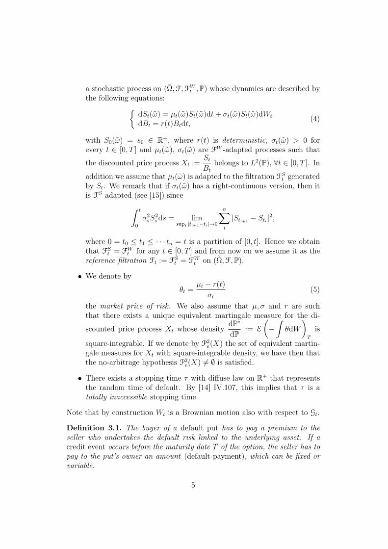
a stochastic process on (Ω,F,FWt ,P) whose dynamics are described by

the following equations:dSt(ω) = µt(ω)St(ω)dt+ σt(ω)St(ω)dWt

dBt = r(t)Btdt,(4)

with S0(ω) = s0 ∈ R+, where r(t) is deterministic, σt(ω) > 0 forevery t ∈ [0, T ] and µt(ω), σt(ω) are FW -adapted processes such that

the discounted price process Xt :=St

Bt

belongs to L2(P), ∀t ∈ [0, T ]. In

addition we assume that µt(ω) is adapted to the filtration FSt generated

by St. We remark that if σt(ω) has a right-continuous version, then itis FS-adapted (see [15]) since∫ t

0

σ2sS

2sds = lim

supi |ti+1−ti|→0

n∑i

|Sti+1− Sti|2,

where 0 = t0 ≤ t1 ≤ · · · tn = t is a partition of [0, t]. Hence we obtainthat FS

t = FWt for any t ∈ [0, T ] and from now on we assume it as the

reference filtration Ft := FSt = FW

t on (Ω,F,P).

• We denote by

θt =µt − r(t)

σt

(5)

the market price of risk. We also assume that µ, σ and r are suchthat there exists a unique equivalent martingale measure for the di-

scounted price process Xt whose densitydP∗

dP:= E

(−∫

θdW

)T

is

square-integrable. If we denote by P2e(X) the set of equivalent martin-

gale measures for Xt with square-integrable density, we have then thatthe no-arbitrage hypothesis P2

e(X) 6= ∅ is satisfied.

• There exists a stopping time τ with diffuse law on R+ that representsthe random time of default. By [14] IV.107, this implies that τ is atotally inaccessible stopping time.

Note that by construction Wt is a Brownian motion also with respect to Gt.

Definition 3.1. The buyer of a default put has to pay a premium to theseller who undertakes the default risk linked to the underlying asset. If acredit event occurs before the maturity date T of the option, the seller has topay to the put’s owner an amount (default payment), which can be fixed orvariable.

5

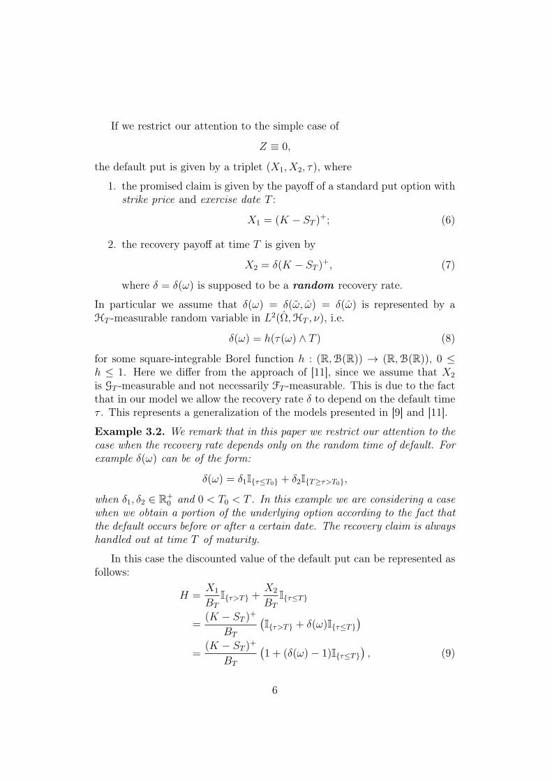
If we restrict our attention to the simple case of

Z ≡ 0,

the default put is given by a triplet (X1, X2, τ), where

1. the promised claim is given by the payoff of a standard put option withstrike price and exercise date T :

X1 = (K − ST )+; (6)

2. the recovery payoff at time T is given by

X2 = δ(K − ST )+, (7)

where δ = δ(ω) is supposed to be a random recovery rate.

In particular we assume that δ(ω) = δ(ω, ω) = δ(ω) is represented by aHT -measurable random variable in L2(Ω,HT , ν), i.e.

δ(ω) = h(τ(ω) ∧ T ) (8)

for some square-integrable Borel function h : (R,B(R)) → (R,B(R)), 0 ≤h ≤ 1. Here we differ from the approach of [11], since we assume that X2

is GT -measurable and not necessarily FT -measurable. This is due to the factthat in our model we allow the recovery rate δ to depend on the default timeτ . This represents a generalization of the models presented in [9] and [11].

Example 3.2. We remark that in this paper we restrict our attention to thecase when the recovery rate depends only on the random time of default. Forexample δ(ω) can be of the form:

δ(ω) = δ1Iτ≤T0 + δ2IT≥τ>T0,

when δ1, δ2 ∈ R+0 and 0 < T0 < T . In this example we are considering a case

when we obtain a portion of the underlying option according to the fact thatthe default occurs before or after a certain date. The recovery claim is alwayshandled out at time T of maturity.

In this case the discounted value of the default put can be represented asfollows:

H =X1

BT

Iτ>T +X2

BT

Iτ≤T

=(K − ST )

+

BT

(Iτ>T + δ(ω)Iτ≤T

)=

(K − ST )+

BT

(1 + (δ(ω)− 1)Iτ≤T

), (9)

6

where δ is given in (8). Our aim is then to apply three different hedgingmethods for H in this setting:

1. Reduced-Form model;

2. Local-Risk Minimization;

3. Mean-Variance Hedging.

4 Reduced-Form modelIn this section we present the main results that can be obtained through theintensity-based approach to the valuation of defaultable claims and then wesee an application to the case of a default-put. We follow here the approachof [9], [10] and [11].Under the assumption of Section 3 the no-defaultable market is completesince there exists a unique equivalent martingale measure P∗ for the discoun-

ted price process Xt =St

Bt

. See [22] for further details. We put

Q∗ = P∗ ⊗ ν

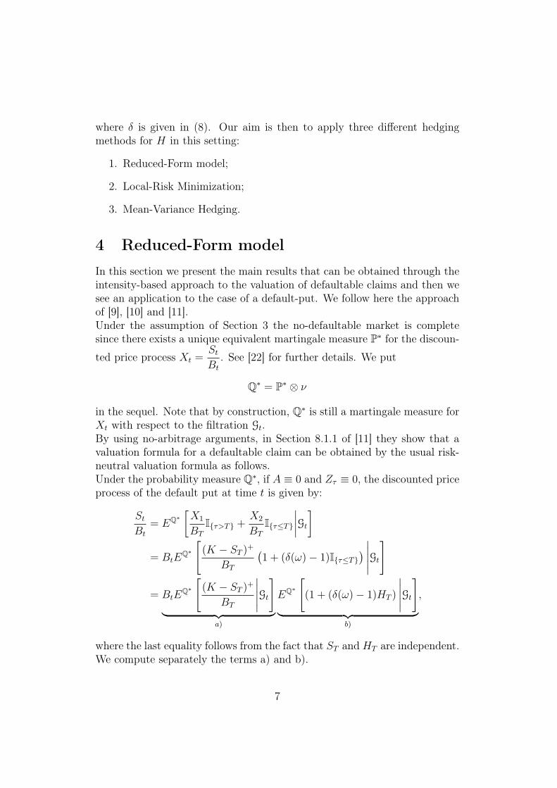
in the sequel. Note that by construction, Q∗ is still a martingale measure forXt with respect to the filtration Gt.By using no-arbitrage arguments, in Section 8.1.1 of [11] they show that avaluation formula for a defaultable claim can be obtained by the usual risk-neutral valuation formula as follows.Under the probability measure Q∗, if A ≡ 0 and Zτ ≡ 0, the discounted priceprocess of the default put at time t is given by:

St

Bt

= EQ∗[X1

BT

Iτ>T +X2

BT

Iτ≤T

∣∣∣∣Gt

]= BtE

Q∗

[(K − ST )

+

BT

(1 + (δ(ω)− 1)Iτ≤T

) ∣∣∣∣∣Gt

]

= BtEQ∗

[(K − ST )

+

BT

∣∣∣∣∣Gt

]︸ ︷︷ ︸

a)

EQ∗

[(1 + (δ(ω)− 1)HT )

∣∣∣∣∣Gt

]︸ ︷︷ ︸

b)

,

where the last equality follows from the fact that ST and HT are independent.We compute separately the terms a) and b).

7

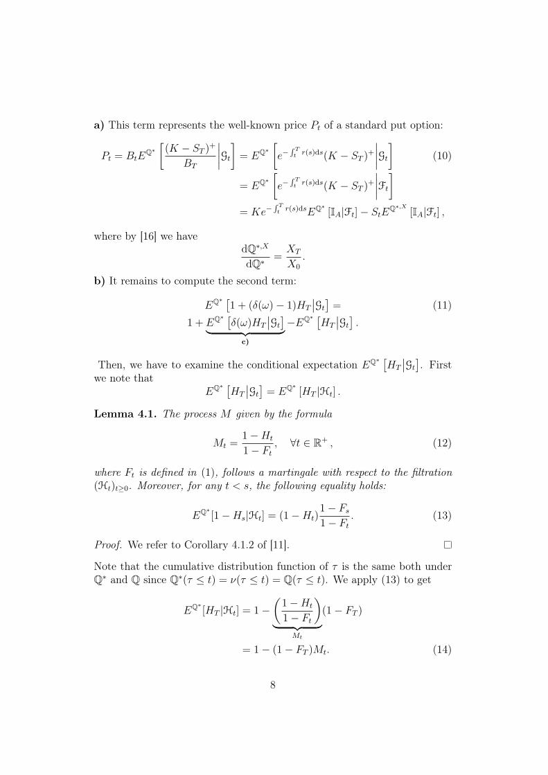
a) This term represents the well-known price Pt of a standard put option:

Pt = BtEQ∗[(K − ST )

+

BT

∣∣∣∣Gt

]= EQ∗

[e−

∫ Tt r(s)ds(K − ST )

+

∣∣∣∣Gt

](10)

= EQ∗[e−

∫ Tt r(s)ds(K − ST )

+

∣∣∣∣Ft

]= Ke−

∫ Tt r(s)dsEQ∗

[IA|Ft]− StEQ∗,X

[IA|Ft] ,

where by [16] we havedQ∗,X

dQ∗ =XT

X0

.

b) It remains to compute the second term:

EQ∗ [1 + (δ(ω)− 1)HT

∣∣Gt

]= (11)

1 + EQ∗ [δ(ω)HT

∣∣Gt

]︸ ︷︷ ︸c)

−EQ∗ [HT

∣∣Gt

].

Then, we have to examine the conditional expectation EQ∗ [HT

∣∣Gt

]. First

we note thatEQ∗ [

HT

∣∣Gt

]= EQ∗

[HT |Ht] .

Lemma 4.1. The process M given by the formula

Mt =1−Ht

1− Ft

, ∀t ∈ R+ , (12)

where Ft is defined in (1), follows a martingale with respect to the filtration(Ht)t≥0. Moreover, for any t < s, the following equality holds:

EQ∗[1−Hs|Ht] = (1−Ht)

1− Fs

1− Ft

. (13)

Proof. We refer to Corollary 4.1.2 of [11].

Note that the cumulative distribution function of τ is the same both underQ∗ and Q since Q∗(τ ≤ t) = ν(τ ≤ t) = Q(τ ≤ t). We apply (13) to get

EQ∗[HT |Ht] = 1−

(1−Ht

1− Ft

)︸ ︷︷ ︸

Mt

(1− FT )

= 1− (1− FT )Mt. (14)

8

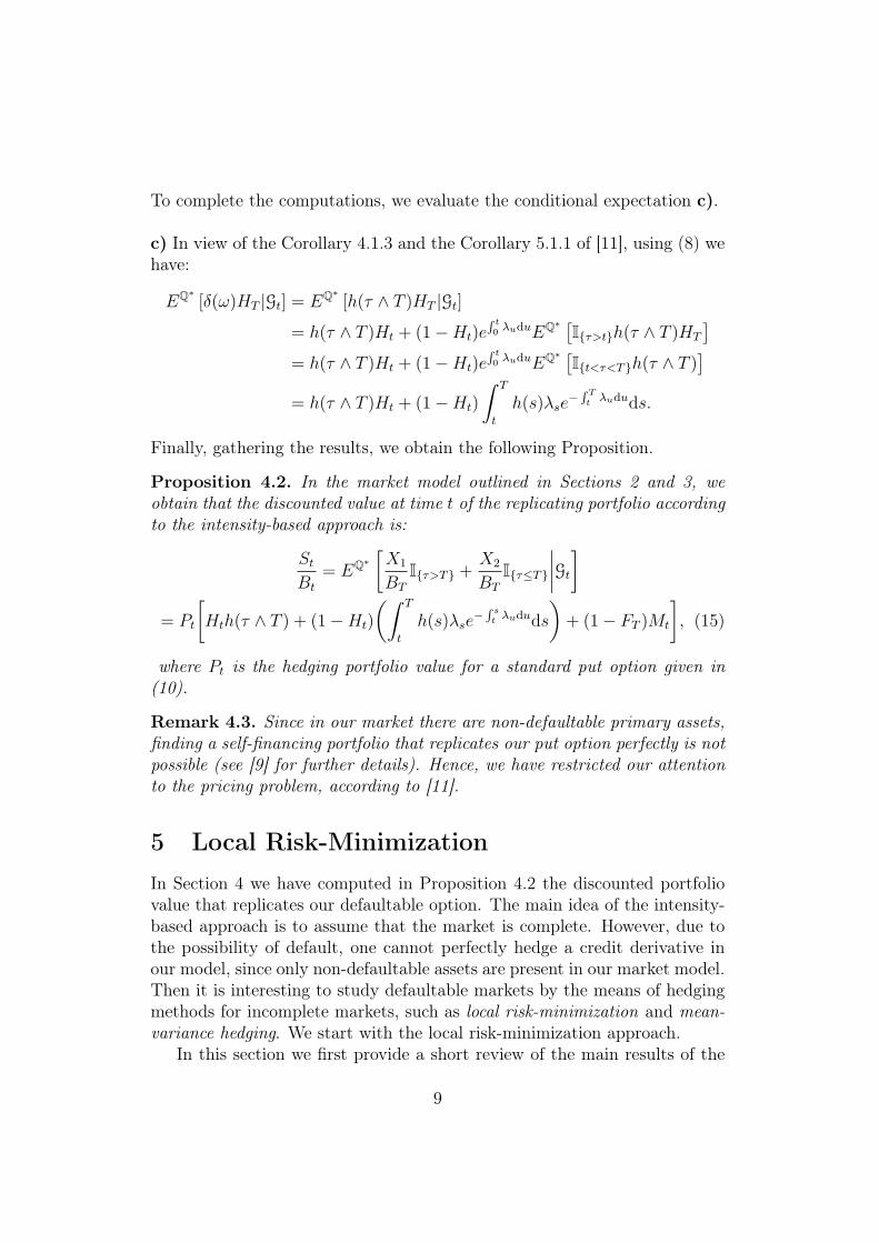
To complete the computations, we evaluate the conditional expectation c).

c) In view of the Corollary 4.1.3 and the Corollary 5.1.1 of [11], using (8) wehave:

EQ∗[δ(ω)HT |Gt] = EQ∗

[h(τ ∧ T )HT |Gt]

= h(τ ∧ T )Ht + (1−Ht)e∫ t0 λuduEQ∗ [Iτ>th(τ ∧ T )HT

]= h(τ ∧ T )Ht + (1−Ht)e

∫ t0 λuduEQ∗ [It<τ<Th(τ ∧ T )

]= h(τ ∧ T )Ht + (1−Ht)

∫ T

t

h(s)λse−

∫ Tt λududs.

Finally, gathering the results, we obtain the following Proposition.

Proposition 4.2. In the market model outlined in Sections 2 and 3, weobtain that the discounted value at time t of the replicating portfolio accordingto the intensity-based approach is:

St

Bt

= EQ∗[X1

BT

Iτ>T +X2

BT

Iτ≤T

∣∣∣∣Gt

]= Pt

[Hth(τ ∧ T ) + (1−Ht)

(∫ T

t

h(s)λse−

∫ st λududs

)+ (1− FT )Mt

], (15)

where Pt is the hedging portfolio value for a standard put option given in(10).

Remark 4.3. Since in our market there are non-defaultable primary assets,finding a self-financing portfolio that replicates our put option perfectly is notpossible (see [9] for further details). Hence, we have restricted our attentionto the pricing problem, according to [11].

5 Local Risk-MinimizationIn Section 4 we have computed in Proposition 4.2 the discounted portfoliovalue that replicates our defaultable option. The main idea of the intensity-based approach is to assume that the market is complete. However, due tothe possibility of default, one cannot perfectly hedge a credit derivative inour model, since only non-defaultable assets are present in our market model.Then it is interesting to study defaultable markets by the means of hedgingmethods for incomplete markets, such as local risk-minimization and mean-variance hedging. We start with the local risk-minimization approach.

In this section we first provide a short review of the main results of the

9

theory of local-risk minimization (see [15], [17], [25]) and then we see an ap-plication in the case of a default-put. The main feature of this approach isthe fact that one has to work with strategies which are not self-financing.

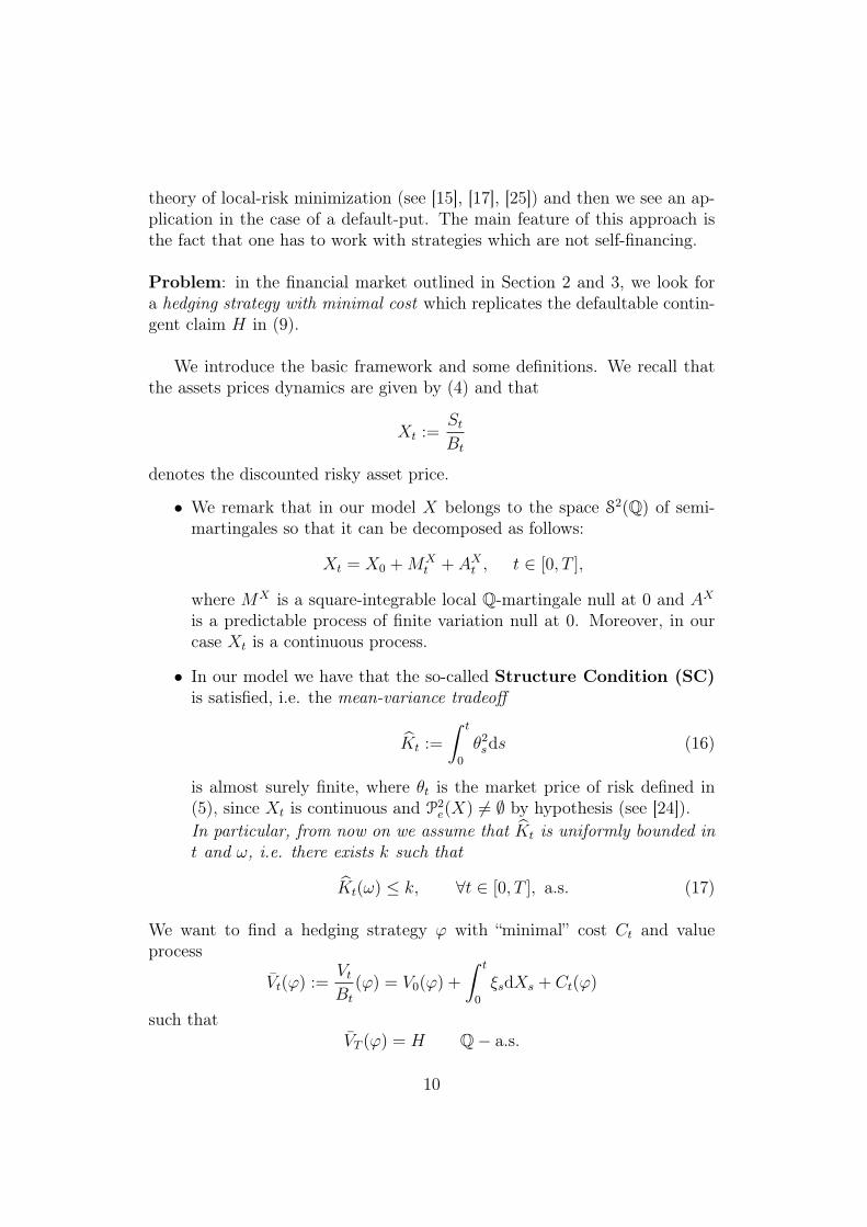
Problem: in the financial market outlined in Section 2 and 3, we look fora hedging strategy with minimal cost which replicates the defaultable contin-gent claim H in (9).

We introduce the basic framework and some definitions. We recall thatthe assets prices dynamics are given by (4) and that

Xt :=St

Bt

denotes the discounted risky asset price.

• We remark that in our model X belongs to the space S2(Q) of semi-martingales so that it can be decomposed as follows:

Xt = X0 +MXt + AX

t , t ∈ [0, T ],

where MX is a square-integrable local Q-martingale null at 0 and AX

is a predictable process of finite variation null at 0. Moreover, in ourcase Xt is a continuous process.

• In our model we have that the so-called Structure Condition (SC)is satisfied, i.e. the mean-variance tradeoff

Kt :=

∫ t

0

θ2sds (16)

is almost surely finite, where θt is the market price of risk defined in(5), since Xt is continuous and P2

e(X) 6= ∅ by hypothesis (see [24]).In particular, from now on we assume that Kt is uniformly bounded int and ω, i.e. there exists k such that

Kt(ω) ≤ k, ∀t ∈ [0, T ], a.s. (17)

We want to find a hedging strategy ϕ with “minimal” cost Ct and valueprocess

Vt(ϕ) :=Vt

Bt

(ϕ) = V0(ϕ) +

∫ t

0

ξsdXs + Ct(ϕ)

such thatVT (ϕ) = H Q− a.s.

10

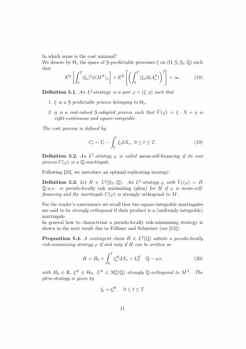
In which sense is the cost minimal?We denote by Θs the space of G-predictable processes ξ on (Ω,G,Gt,Q) suchthat

EQ[∫ T

0

(ξs)2d〈MX〉s

]+ EQ

[(∫ T

0

|ξs|d|AXs |)2]< ∞. (18)

Definition 5.1. An L2-strategy is a pair ϕ = (ξ, η) such that

1. ξ is a G-predictable process belonging to Θs.

2. η is a real-valued G-adapted process such that V (ϕ) = ξ · X + η isright-continuous and square-integrable.

The cost process is defined by:

Ct = Vt −∫ t

0

ξsdXs, 0 ≤ t ≤ T. (19)

Definition 5.2. An L2-strategy ϕ is called mean-self-financing if its costprocess C(ϕ) is a Q-martingale.

Following [25], we introduce an optimal replicating strategy:

Definition 5.3. Let H ∈ L2(GT ,Q). An L2-strategy ϕ with VT (ϕ) = HQ-a.e. is pseudo-locally risk minimizing (plrm) for H if ϕ is mean-self-financing and the martingale C(ϕ) is strongly orthogonal to M .

For the reader’s convenience we recall that two square-integrable martingalesare said to be strongly orthogonal if their product is a (uniformly integrable)martingale.In general how to characterize a pseudo-locally risk-minimizing strategy isshown in the next result due to Föllmer and Schweizer (see [15]):

Proposition 5.4. A contingent claim H ∈ L2(Q) admits a pseudo-locallyrisk-minimizing strategy ϕ if and only if H can be written as

H = H0 +

∫ T

0

ξHs dXs + LHT Q− a.s. (20)

with H0 ∈ R, ξH ∈ ΘS, LH ∈ M20(Q) strongly Q-orthogonal to MX . The

plrm-strategy is given by

ξt = ξHt , 0 ≤ t ≤ T

11

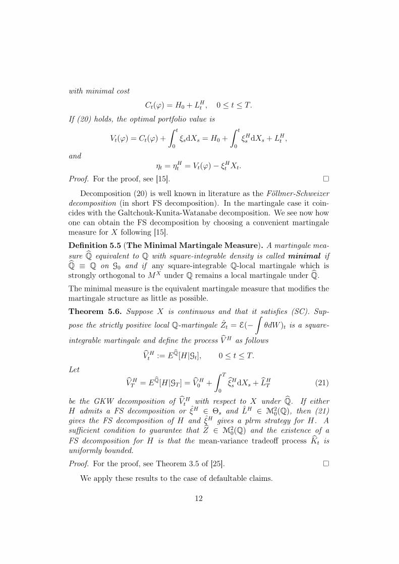
with minimal cost

Ct(ϕ) = H0 + LHt , 0 ≤ t ≤ T.

If (20) holds, the optimal portfolio value is

Vt(ϕ) = Ct(ϕ) +

∫ t

0

ξsdXs = H0 +

∫ t

0

ξHs dXs + LHt ,

andηt = ηHt = Vt(ϕ)− ξHt Xt.

Proof. For the proof, see [15].

Decomposition (20) is well known in literature as the Föllmer-Schweizerdecomposition (in short FS decomposition). In the martingale case it coin-cides with the Galtchouk-Kunita-Watanabe decomposition. We see now howone can obtain the FS decomposition by choosing a convenient martingalemeasure for X following [15].

Definition 5.5 (The Minimal Martingale Measure). A martingale mea-sure Q equivalent to Q with square-integrable density is called minimal ifQ ≡ Q on G0 and if any square-integrable Q-local martingale which isstrongly orthogonal to MX under Q remains a local martingale under Q.

The minimal measure is the equivalent martingale measure that modifies themartingale structure as little as possible.

Theorem 5.6. Suppose X is continuous and that it satisfies (SC). Sup-

pose the strictly positive local Q-martingale Zt = E(−∫

θdW )t is a square-

integrable martingale and define the process V H as follows

V Ht := EQ[H|Gt], 0 ≤ t ≤ T.

Let

V HT = EQ[H|GT ] = V H

0 +

∫ T

0

ξHs dXs + LHT (21)

be the GKW decomposition of V Ht with respect to X under Q. If either

H admits a FS decomposition or ξH ∈ Θs and LH ∈ M20(Q), then (21)

gives the FS decomposition of H and ξH gives a plrm strategy for H. Asufficient condition to guarantee that Z ∈ M2

0(Q) and the existence of aFS decomposition for H is that the mean-variance tradeoff process Kt isuniformly bounded.

Proof. For the proof, see Theorem 3.5 of [25].

We apply these results to the case of defaultable claims.

12

5.1 Local-Risk-Minimization for defaultable claims

We focus on the particular case of a default put H defined in (9). For localrisk minimization for a general defaultable claim, we refer to [1]. We wish tofind a portfolio “with minimal cost” that perfectly replicates H according tothe local risk-minimizing criterion.We remark that we focus on the case of trading strategies adapted to the fullfiltration Gt (see [9]). For a further discussion on local risk-minimization withFt-adapted strategies, we refer to [2].

Lemma 5.7. The minimal martingale measure for Xt with respect to Gt

exists and coincides with Q∗.

Proof. Since Wt and Mt defined in (2) have the predictable representationproperty for the space of square-integrable local martingale on the productprobability space (Ω,G,Gt,Q) = (Ω× Ω,FW ⊗H,FW

t ⊗Ht,P⊗ν), the resultfollows by Definition 5.5. See also [3] and [20].

Proposition 5.8. Let M be the compensated process defined in (2) and X thediscounted price process. The pair (X, M) has the predictable representationproperty on (Ω,G,Gt,Q∗), i.e. for every H ∈ L1(Ω,GT ,Q∗), there exists apair of G-predictable processes (Φ, Ψ) such that

H = c+

∫ T

0

ΦsdXs +

∫ T

0

ΨsdMs (22)

and ∫ T

0

Φ2sd〈X〉s +

∫ T

0

Ψ2sd[M ]s < ∞ a.s.

Proof. Since there exists a unique equivalent martingale measure P∗ for thecontinuous asset process Xt on (Ω,F,Ft), then by Theorem 40 of Chapter IVof [21] we have that Xt has the predictable representation property for thelocal martingales on (Ω,F,Ft,P∗).By Proposition 4.1 of [4] the compensated default process Mt has the pre-dictable representation property for the local martingales on (Ω,H,Ht, ν).Hence, since Xt and Mt are strongly orthogonal, by Proposition A.2 of [3]and by using a limiting argument we obtain that (X, M) has the predictablerepresentation property on the product probability space

(Ω,G,Gt,Q∗) = (Ω× Ω,F ⊗H,Ft ⊗Ht,P∗ ⊗ ν).

13

We remark that the market is incomplete even if we trade with Gt-adaptedstrategies since M does not represent the value of any tradable asset.We can apply Proposition 5.8 to obtain the plrm strategy for H ∈ L2(Ω,GT ,Q).

Proposition 5.9. Let H ∈ L2(Ω,GT ,Q) be the value of a defaultable claim.Then the plrm strategy for H exists and it is given by

Φt = Φt, Ct = c+

∫ t

0

ΨsdMs,

where Φt, Ψt are the same as in Proposition 5.8.

Proof. Let H ∈ L2(Ω,GT ,Q). We note that sincedQdQ

∈ L2(Q), then

L2(Ω,GT ,Q) ⊂ L1(Ω,GT , Q). Then H ∈ L1(Q) and we can apply Propo-sition 5.8 to obtain decomposition (22) for H given by

H = c+

∫ T

0

ΦsdXs +

∫ T

0

ΨsdMs. (23)

The martingale M is strongly orthogonal to the martingale part MX of X,hence (23) gives the GKW decomposition of H under Q. Since by hypothesisdQdQ

=dQ∗

dQ∈ L2(Q) and Xt is continuous, then by Theorem 3.5 of [15] the

associated density process

Zt = EQ

[dQdQ

∣∣∣∣Gt

]= EQ

[dQdQ

∣∣∣∣Ft

]

is a square-integrable martingale. Since hypothesis (17) is in force, we canapply Theorem 5.6 and conclude that (22) is the FS decomposition of H.

Remark 5.10. It is possible to choose different hypotheses that guaranteethat decomposition (22) gives the FS decomposition. Assumption (17) isthe simplest condition that can be assumed. For a complete survey and adiscussion of the others, we refer to [25].

Under the equivalent martingale probability measure Q, the discounted price

14

process Vt of the default put at time t, is given by:

Vt = EQ[H|Gt]

= EQ[X1

BT

Iτ>T +X2

BT

Iτ≤T

∣∣∣∣Gt

]= EQ

[X1

BT

∣∣∣∣Gt

]· EQ

[1 + (δ(ω)− 1)HT

∣∣∣∣Gt

]= EQ

[(K − ST )

+

BT

∣∣∣∣∣Gt

]︸ ︷︷ ︸

a)

·EQ

[(1 + (δ(ω)− 1)HT )

∣∣∣∣∣Gt

]︸ ︷︷ ︸

b)

. (24)

We need only to find the Föllmer-Schweizer decomposition of Vt as illustratedin (20).

a) By Section 5 of [5] and using the “change of numéraire” technique of[16], we have

EQ[X1

BT

∣∣∣∣Gt

]= EQ

[(K − ST )

+

BT

∣∣∣∣Gt

]

= EQ

(K − ST )

BT

IK ≥ ST︸ ︷︷ ︸A

∣∣∣∣Gt

= KEQ

[1

BT

IA∣∣∣∣Gt

]− EQ

[ST

BT

IA∣∣∣∣Gt

]=

K

BT

EQ [IA∣∣Gt

]− EQ[XT IA|Gt]

=K

BT

EQ [IA|Gt]−XtEQX

[IA|Gt] ,

wheredQX

dQ=

XT

X0

is well-defined since XT ∈ L2(Q) by hypothesis and hence XT ∈ L1(Q).

In addition by (22) we obtain that EQ[X1

BT

∣∣∣∣Gt

]admits the decompo-

sition

EQ[X1

BT

∣∣∣∣Gt

]= c+

∫ t

0

ξsdXs. (25)

15

SinceEQX

[IA|Gt] = EQX

[IA|Ft]

because IA is independent of τ , by [16] we have that

ξt = EQX

[IA|Ft] . (26)

b) It remains to calculate the term EQ[1 + (δ(ω)− 1)HT

∣∣∣∣Gt

]. First we

note that

EQ[1 + (δ(ω)− 1)HT

∣∣∣∣Gt

]= 1 + EQ[δ(ω)HT |Gt]− EQ[HT |Gt]

= 1 + EQ[δ(ω)HT |Gt]− (1− (1− FT )Mt)

= EQ[δ(ω)HT |Gt] + (1− FT )Mt,

by (14). Since δ(ω)HT = f(τ) for some integrable Borel function f :R+ → [0, 1], by Proposition 4.3.1 of [11], we have

EQ[1 + (δ(ω)− 1)HT

∣∣∣∣Gt

]= ch +

∫ t

0

f(s)dMs + (1− FT )Mt,

where ch = EQ[f(τ)] and the function f : R+ → R is given by theformula

f(t) = f(t)− eΓtEQ[Iτ>tf(τ)]. (27)

Note thatf(x) = h(x ∧ T )Ix<T,

where h is introduced in (8). We only need to find the relationshipbetween Mt and Mt.

Lemma 5.11. Let M and M be defined by (2) and (12) respectively.The following equality holds:

dMt = − 1

1− Ft

dMt. (28)

Proof. To obtain (28), it suffices to apply Itô’s formula. For furtherdetails see Section 6.3 of [11].

16

Finally, gathering the results we obtain

Vt = EQ[H|Gt]

=

c+

∫ t

0

ξsdXs︸ ︷︷ ︸Φt

·(EQ[f(τ)] +

∫ t

0

f(s)dMs + (1− FT )Mt

)

= Φt ·

EQ[f(τ)] +

∫ t

0

(f(s)− 1− FT

1− Fs

)dMs︸ ︷︷ ︸

Ψt

.

Sinced[Φ,Ψ]t = ξt

(f(t)− 1− FT

1− Ft

)d[X, M ]t = 0,

applying Itô’s formula we get

dVt = ΦtdΨt +Ψt−dΦt + d[Φ,Ψ]t

=

(c+

∫ t

0

ξsdXs

)(f(t)− 1− FT

1− Ft

)dMt +

(EQ[f(τ)] +

∫ t

0

(f(s)+

− 1− FT

1− Fs

)dMs

)ξtdXt.

(29)

Hence we can conclude that:

Proposition 5.12. In the market model outlined in Sections 2 and 3, underhypothesis (17) the local risk-minimizing portfolio for H defined in (9) isgiven by

Vt = c1 +

∫ t

0

Φ1sdXs + Lt, (30)

where the plrm strategy is

Φ1t =

(EQ[f(τ)] +

∫ t

0

(f(s)− 1− FT

1− Fs

)dMs

)ξt (31)

and the minimal cost is

Lt =

∫ t

0

(c+

∫ s

0

ξudXu

)(f(s)− 1− FT

1− Fs

)dMs, (32)

where ξt is given by (26), f(s) by (27) and Ft by (1).

Proof. Proposition 5.9 guarantees that (29) provides the FS decompositionfor H, i.e. that Φ1

t and Lt satisfy the required integrability conditions.

17

6 Mean-Variance HedgingFinally we consider the mean-variance hedging approach. We refer to [25]for an exhaustive survey of relevant results. This method has been alreadyapplied to defaultable markets in [6], [7], [8] and [9]. Here we extend theirresults to the case of general coefficients in the dynamics of Xt and randomrecovery rate and compute explicitly the mean-variance strategy in the par-ticular case of a put option.Again we focus on the case of G-adapted hedging strategy and denote byL(X) the set of all G-predictable X-integrable processes.

Definition 6.1. An admissible hedging strategy is any pair ϕ = (θ, η), whereθ is a G-predictable process in L(X) and η is a real-valued G-adapted process

such that the discounted value process Vt(ϕ) :=Vt

Bt

(ϕ) = ηt+θtXt, 0 ≤ t ≤ T

is right-continuous.

Note that if the discounted value process V (ϕ) is self-financing - that is

Vt(ϕ) = V0 +

∫ t

0

θsdXs, then η is completely determined by the pair (V0, θ):

ηt = V0 +

∫ t

0

θsdXs − θtXt, 0 ≤ t ≤ T.

Hence we can formulate the mean-variance problem as follows:Problem: find an admissible strategy (V0, θ) which solves the following mi-nimization problem:

min(V0,θ)

E

[(H − V0 −

∫ T

0

θsdXs

)2],

where θ belongs to

Θ =

θ ∈ L(X) :

∫ t

0

θsdXs ∈ S2(Q)

.

If such strategy exists, it is called Mean-Variance Optimal Strategy and de-noted by (V0, θ).Dual Problem: find an equivalent martingale measure Q such that its den-sity is square-integrable and its norm:∥∥∥∥∥dQdQ

∥∥∥∥∥2

= E

(dQdQ

)2

18

is minimal over all the probability measures in P2e(X). By [13] this probability

measure exists since Xt is continuous and P2e 6= ∅ and it is called Variance-

Optimal Measure since: ∥∥∥∥∥dQdQ∥∥∥∥∥2

= 1 + V ar

[dQdQ

].

The main result is given by the following Theorem:

Theorem 6.2. Suppose Θ is closed and let X be a continuous process suchthat P2

e(X) 6= ∅. Let H ∈ L2(Q) be a contingent claim and write theGaltchouk-Kunita-Watanabe decomposition of H under Q with respect to Xas

H = EQ[H] +

∫ T

0

ξHu dXu + LT = VT , (33)

with

Vt := EQ[H|Gt] = EQ[H] +

∫ t

0

ξHu dXu + Lt, 0 ≤ t ≤ T. (34)

Then the mean-variance optimal Θ-strategy for H exists and it is given by

V0 = EQ[H]

and

θt = ξHt − ζt

Zt

(Vt− − EQ[H]−

∫ t

0

θudXu

)= ξHt − ζt

(V0 − EQ[H]

Z0

+

∫ t−

0

1

Zu

dLu

), 0 ≤ t ≤ T,

where

Zt = EQ

[dQdQ

∣∣∣∣Gt

]= Z0 +

∫ t

0

ζudXu, 0 ≤ t ≤ T (35)

Proof. The proof can be found in [23].

Let us now turn to the case of the default put. We can interpret the presenceon the market of a default possibility as a particular case of “incompleteinformation”. Hence the results of [3] and [4], where the variance-optimalmeasure is characterized as the solution of an equation between Doléansexponentials, can also be applied in this context to compute Q. In particular

19

by [3], Theorem 2.16 and Section 3 (α), it follows that the variance-optimalmeasure coincides with the minimal one. In this case

Q = Q = Q∗. (36)

First of all we check that the space Θ is closed.By Proposition 4.2 of [3], we have that Θ is closed if and only if for everystopping time η, with 0 ≤ η ≤ T , the following condition holds

EQ[exp

(∫ T

η

θ2sds

) ∣∣∣∣Gη

]≤ M, (37)

wheredQdQ

:= E

(−∫

2θdW

)T

. Note that since we are assuming that Q

exists and it is square-integrable, then Q also exists and exp(∫ T

0θ2t dt

)is Q-

integrable ([3], Section 3(α)). Here we obtain that condition (37) is a verifiedfor every G-stopping time η such that 0 ≤ η ≤ T as a consequence of ourassumption (17). Then we can use Theorem 6.2 to obtain the mean-varianceoptimal Θ-strategy for H.The process Vt at time t, is given by:

Vt = EQ[H|Gt]

= EQ[X1

BT

Iτ>T +X2

BT

Iτ≤T

∣∣∣∣Gt

]= EQ

[(K − ST )

+

BT

(1 + (δ(ω)− 1)Iτ≤T

) ∣∣∣∣∣Gt

].

By Section 3 (α) in [3], we also obtain that

dQdQ

= E

(−∫

βdX

)T

1

E [(−βdX)],

where βt =θt − ht

σtXt

and ht solves the equation

E

(∫hdW

)T

=exp(

∫ T

0θ2t dt)

E[exp

(∫ T

0θ2t dt

)]with Wt := Wt + 2

∫ t

0θsds and dQ

dQ = E(−∫2θdW

)T. Hence we have that

Zt = EQ

[dQdQ

∣∣∣∣Ft

]=

E(−∫βdX

)t

E[E(−∫βdX

)T

] (38)

20

and dZt = βtZtdXt. Consequently we can compute decomposition (35) andobtain

ζt = Ztβt. (39)

Since Q = Q = Q∗, we can use (30), (31) and (32), to obtain the mean-variance optimal Θ-strategy (V0, θ) for H.

Proposition 6.3. In the market model outlined in Sections 2 and 3, underhypothesis (17) the mean-variance hedging strategy for H defined in (9) isgiven by:

• Optimal Price

V0 = EQ[H] = EQ[X1

BT

Iτ>T +X2

BT

Iτ≤T

].

We note that the optimal price for the mean-variance hedging criterioncoincides with the optimal price for the locally risk-minimizing crite-rion.

• Mean-Variance Optimal Strategy

θt = Φ1t − ζt

∫ t−

0

1

Zu

dLu, (40)

where Φ1, Z and ζ are given by (31), (38) and (39) respectively and

dLt = dLt =

(c+

∫ t

0

ξsdXs

)(f(t)− 1− FT

1− Ft

)dMt. (41)

Acknowledgements

We thank Damir Filipović, Ian Kallsen and Martin Schweizer for intere-sting discussions and remarks.

References[1] Biagini F., Cretarola A. (2006) “Local Risk-Minimization for Defaulta-

ble Markets”, preprint, LMU University of München and University ofBologna.

[2] Biagini F., Cretarola A. (2006) “Local Risk-Minimization for DefaultableClaims with Recovery Process”, preprint, LMU University of Münchenand University of Bologna.

21

[3] Biagini F., Guasoni P., Pratelli M. (2000) “Mean-Variance Hedging forStochastic Volatility Models ”, Mathematical Finance, vol.10, number 2,109-123.

[4] Biagini F., Guasoni P. (2002) “Mean-Variance Hedging with randomvolatility jumps”, Stochastic Analysis and Applications 20, 471-494.

[5] Biagini F., Pratelli M. (1999) “Local Risk Minimization and Numéraire”,Journal of Applied Probability, vol.36, number 4, 1-14.

[6] Bielecki T.R., Jeanblanc M. (2004) “Indifference Pricing of Defaulta-ble Claims”, In Indifference pricing, Theory and Applications, FinancialEngineering, Princeton University Press.

[7] Bielecki T.R., Jeanblanc M., Rutkowski M. (2004) “Pricing and Hedgingof Credit Risk: Replication and Mean- Variance Approaches I ”, Mathe-matics of finance, Contemp. Math., 351, Amer. Math. Soc., Providence,RI, 37-53.

[8] Bielecki T.R., Jeanblanc M., Rutkowski M. (2004) “Pricing and Hedgingof Credit Risk: Replication and Mean- Variance Approaches II ”, Mathe-matics of finance, Contemp. Math., 351, Amer. Math. Soc., Providence,RI, 55-64.

[9] Bielecki T.R., Jeanblanc M., Rutkowski M. (2004) “Hedging of Defaul-table Claims”, Paris-Princeton Lectures on Mathematical Finance 2003,Lecture Notes in Mathematics 1847, Springer, Berlin.

[10] Bielecki T.R., Jeanblanc M., Rutkowski M. (2004) “Modelling and Val-uation of Credit Risk ”, Stochastic methods in finance, Lecture Notes inMath., 1856, Springer, Berlin, 27-126.

[11] Bielecki T.R., Rutkowski M. (2004) “Credit Risk: Modelling, Valuationand Hedging”, Second edition, Springer.

[12] Covitz D., Han S. (2004) “An Empirical Analysis of Bond RecoveryRates: Exploring a Structural View of Default”, The Federal ReserveBoard, Washington, Preprint.

[13] Delbaen F., Schachermayer W. (1996a) “The Variance-Optimal Martin-gale Measure for Continuous Processes”, Bernoulli 2, 81-105; amend-ments and corrections (1996), Bernoulli 2, 379-80.

[14] Dellacherie C., Meyer P.A. (1982) “Probabilities and Potential B: Theoryof Martingales”, Amsterdam: North Holland.

22

[15] Föllmer H., Schweizer M. (1991) “Hedging of contingent claims underincomplete information”, in: R.J. Eliot and M.H.A. Davis, editors, Ap-plied Stochastic Analysis, 389-414. Gordon and Breach.

[16] Geman H., El Karoui N., Rochet J.C. (1995) “Changes of Numéraire,changes of probability measure and option pricing”, J. App. Prob. 32,443-458.

[17] Heath D., Platen E., Schweizer M. (2001) “A Comparison of TwoQuadratic Approaches to Hedging in Incomplete Markets” MathematicalFinance 11, 385-413.

[18] Heath D., Platen E., Schweizer M. (2001) “Numerical Comparison ofLocal Risk-Minimization and Mean-Variance Hedging” in: E. Jouini, J.Cvitanic, M. Musiela (eds.), “Option Pricing, Interest Rates and RiskManagement”, Cambridge University Press , 509-537.

[19] Lamberton D., Lapeyre B. (1996) “Introduction to Stochastic CalculusApplied to Finance”, Chapman-Hall.

[20] Møller T. (2001) “Risk-minimizing Hedging Strategies for Insurance Pay-ment Processes”, Finance and Stochastics 5, 419-446.

[21] Protter P. (1990) “Stochastic Integration and Differential Equations”,Applications of Mathematics, Springer-Verlag Berlin Heidelberg.

[22] Øksendal B. (1998) “Stochastic Differential Equations”, Springer-Verlag,Berlin Heidelberg.

[23] Rheinländer T., Schweizer M. (1997) “On L2-Projections on a Space ofStochastic Integrals”, Annals of Probability 25, 1810-31.

[24] Schweizer M. (1995) “On the Minimal Martingale Measure and theFöllmer-Schweizer Decomposition”, Stochastic Analysis and Applica-tions 13, 573-599.

[25] Schweizer M. (2001) “A Guided Tour through Quadratic Hedging Ap-proaches” in: E. Jouini, J. Cvitanic, M. Musiela (eds.), “Option Pricing,Interest Rates and Risk Management”, Cambridge University Press, 538-574.

23