Embed Size (px)
Citation preview
Quadrotor Implementation of the Three-Dimensional Distributed ReactiveCollision Avoidance Algorithm
Esther Anderson
A thesis submitted in partial fulfillment ofthe requirements for the degree of
Master of Science in Aeronautics and Astronautics
University of Washington
2011
Program Authorized to Offer Degree: Aeronautics and Astronautics

University of WashingtonGraduate School
This is to certify that I have examined this copy of a master’s thesis by
Esther Anderson
and have found that it is complete and satisfactory in all respects,and that any and all revisions required by the final
examining committee have been made.
Committee Members:
Kristi A. Morgansen
Juris Vagners
Date:

In presenting this thesis in partial fulfillment of the requirements for a master’s degree at the Univer-sity of Washington, I agree that the Library shall make its copies freely available for inspection. Ifurther agree that extensive copying of this thesis is allowable only for scholarly purposes, consistentwith “fair use” as prescribed in the U.S. Copyright Law. Any other reproduction for any purpose orby any means shall not be allowed without my written permission.
Signature
Date

University of Washington
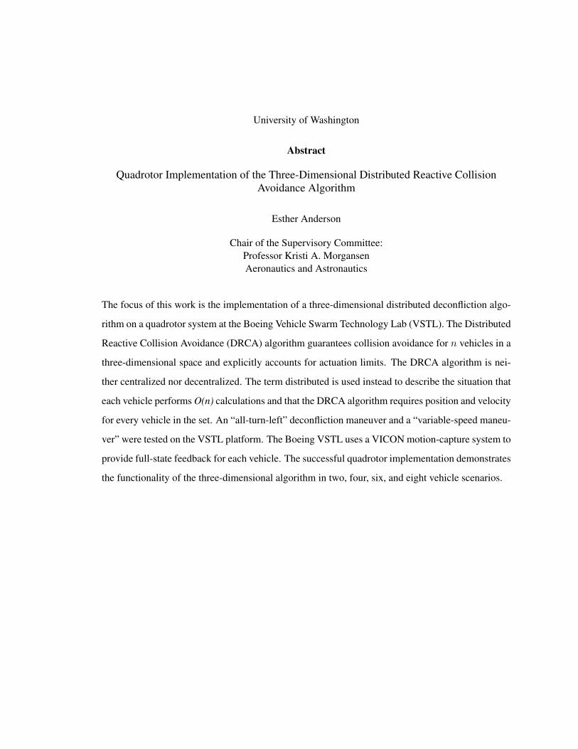
Abstract
Quadrotor Implementation of the Three-Dimensional Distributed Reactive CollisionAvoidance Algorithm
Esther Anderson
Chair of the Supervisory Committee:Professor Kristi A. MorgansenAeronautics and Astronautics
The focus of this work is the implementation of a three-dimensional distributed deconfliction algo-
rithm on a quadrotor system at the Boeing Vehicle Swarm Technology Lab (VSTL). The Distributed
Reactive Collision Avoidance (DRCA) algorithm guarantees collision avoidance for n vehicles in a
three-dimensional space and explicitly accounts for actuation limits. The DRCA algorithm is nei-
ther centralized nor decentralized. The term distributed is used instead to describe the situation that
each vehicle performs O(n) calculations and that the DRCA algorithm requires position and velocity
for every vehicle in the set. An “all-turn-left” deconfliction maneuver and a “variable-speed maneu-
ver” were tested on the VSTL platform. The Boeing VSTL uses a VICON motion-capture system to
provide full-state feedback for each vehicle. The successful quadrotor implementation demonstrates
the functionality of the three-dimensional algorithm in two, four, six, and eight vehicle scenarios.

TABLE OF CONTENTS
Page
List of Figures . . . . . . . . . . . . . . . . . . . . . . . . . . . . . . . . . . . . . . . . . . iii
List of Tables . . . . . . . . . . . . . . . . . . . . . . . . . . . . . . . . . . . . . . . . . . v
Chapter 1: Introduction . . . . . . . . . . . . . . . . . . . . . . . . . . . . . . . . . . 1
1.1 Literature Review . . . . . . . . . . . . . . . . . . . . . . . . . . . . . . . . . . . 5
Chapter 2: Quadrotor System . . . . . . . . . . . . . . . . . . . . . . . . . . . . . . . 7
Chapter 3: DRCA Theoretical Work . . . . . . . . . . . . . . . . . . . . . . . . . . . 9
3.1 Collision Cone and Conflict Detection . . . . . . . . . . . . . . . . . . . . . . . . 9
3.2 DRCA Algorithm Description . . . . . . . . . . . . . . . . . . . . . . . . . . . . 12
3.3 Deconfliction Maneuver . . . . . . . . . . . . . . . . . . . . . . . . . . . . . . . 13
3.4 Deconfliction Maintenance . . . . . . . . . . . . . . . . . . . . . . . . . . . . . . 20
Chapter 4: Testbed and Simulation Environment . . . . . . . . . . . . . . . . . . . . . 27
4.1 Testbed Constraints and DRCA . . . . . . . . . . . . . . . . . . . . . . . . . . . . 31
4.2 Test Scenarios . . . . . . . . . . . . . . . . . . . . . . . . . . . . . . . . . . . . . 31
Chapter 5: All-turn-left 2D and 3D Simulation and Flight Test Results . . . . . . . . . 38
5.1 All-turn-left 3D Simulation and Flight Test Results . . . . . . . . . . . . . . . . . 38
5.2 Advantages of the All-Turn-Left Maneuver . . . . . . . . . . . . . . . . . . . . . 43
5.3 All-turn-left 2D Congested Test Space Simulation Results . . . . . . . . . . . . . 46
5.4 Limitations of the All-Turn-Left Maneuver . . . . . . . . . . . . . . . . . . . . . 47
5.5 All-turn-left 2D Overtaking and Hovering Simulation Results . . . . . . . . . . . . 50
Chapter 6: Variable-Speed Maneuver 2D and 3D Simulation . . . . . . . . . . . . . . 55
6.1 Advantages of the Variable-Speed Maneuver . . . . . . . . . . . . . . . . . . . . . 55
6.2 Variable-speed 2D Overtaking and Hovering Simulation Results . . . . . . . . . . 55
6.3 Limitations of the Variable-Speed Maneuver . . . . . . . . . . . . . . . . . . . . . 56
i
6.4 Variable-speed 3D Simulation Results . . . . . . . . . . . . . . . . . . . . . . . . 56
Chapter 7: Conclusion and Future Work . . . . . . . . . . . . . . . . . . . . . . . . . 64
Bibliography . . . . . . . . . . . . . . . . . . . . . . . . . . . . . . . . . . . . . . . . . . 66
ii
LIST OF FIGURES
Figure Number Page
1.1 The 20 Continental U.S. Air Route Traffic Control Centers . . . . . . . . . . . . . 2
1.2 A near-miss incident of a UAV and A300 airplane . . . . . . . . . . . . . . . . . . 3
3.1 Geometric definition of the collision cone. . . . . . . . . . . . . . . . . . . . . . . 10
3.2 DRCA algorithm flow chart. . . . . . . . . . . . . . . . . . . . . . . . . . . . . . 12
3.3 Example of an infeasible variable-speed maneuver problem. . . . . . . . . . . . . 19
3.4 Geometry of the conflict measures pt and pn. . . . . . . . . . . . . . . . . . . . . 20
3.5 Example of the control function, F . Note that P4 increases and decreases withchanging ud. . . . . . . . . . . . . . . . . . . . . . . . . . . . . . . . . . . . . . 22
3.6 Visual illustration of the spring-like buffer, ε. If a vehicle tries to push againstthis buffer towards a conflict, the buffer will push back. The faster a vehicle isaccelerating toward the collision cone, the harder the buffer will push back. . . . . 23
4.1 Vehicle Swarm Technology Laboratory (VSTL) developed by the Boeing Researchand Technology group. . . . . . . . . . . . . . . . . . . . . . . . . . . . . . . . . 28
4.2 Quadrotor vehicle equipped with reference markers. . . . . . . . . . . . . . . . . . 28
4.3 Old control sequence with additive velocity. . . . . . . . . . . . . . . . . . . . . . 30
4.4 New control sequence without additive velocity. . . . . . . . . . . . . . . . . . . . 30
4.5 Code flow of the DRCA algorithm in simulation. . . . . . . . . . . . . . . . . . . 31
4.6 Description of head-on, crossing, and overtaking scenarios. . . . . . . . . . . . . . 32
5.1 Scenario 1: All-turn-left 3D simulation and flight test. . . . . . . . . . . . . . . . . 40
5.2 Scenario 2: All-turn-left 3D simulation and flight test. . . . . . . . . . . . . . . . . 42
5.3 Scenario 3: All-turn-left 3D simulation and flight test. . . . . . . . . . . . . . . . . 44
5.4 Scenario 4: All-turn-left 3D simulation and flight test. . . . . . . . . . . . . . . . . 45
5.5 Scenario 5: All-turn-left 2D 8 vehicle scenario. . . . . . . . . . . . . . . . . . . . 48
5.6 Scenario 6: All-turn-left 2D 6 vehicle repeated waypoint touch-and-go scenario. . . 49
5.7 Scenario 7: All-turn-left 2D 6 vehicle touch-and-go unique waypoint scenario. . . . 52
5.8 Scenario 8: All-turn-left 2D hovering scenario. . . . . . . . . . . . . . . . . . . . 53
5.9 Scenario 9: All-turn-left 2D overtaking scenario. . . . . . . . . . . . . . . . . . . 54
6.1 Scenario 8: Variable-speed 2D hovering scenario. . . . . . . . . . . . . . . . . . . 59
iii
6.2 Scenario 9: Variable-speed 2D overtaking scenario. . . . . . . . . . . . . . . . . . 606.3 Scenario 1: Variable-speed 3D simulation. . . . . . . . . . . . . . . . . . . . . . . 616.4 Scenario 3: Variable-speed 3D simulation. . . . . . . . . . . . . . . . . . . . . . . 626.5 Scenario 4: Variable-speed 3D simulation. . . . . . . . . . . . . . . . . . . . . . . 63
iv
LIST OF TABLES
Table Number Page
4.1 Parameters used in DRCA simulation. . . . . . . . . . . . . . . . . . . . . . . . . 33
v
ACKNOWLEDGMENTS
The author wishes to express heartfelt appreciation to Juris Vagners and Kristi Morgansen for
their guidance and support, Emmett Lalish and Andrew Melander for their previous work and as-
sistance with this project, Christopher Lum for being extremely gracious and answering many of
my questions, and to the rest of the Department of Aeronautics and Astronautics for the superb
education received.
vi

DEDICATION
To my husband Nate
vii

The views expressed in this article are those of the author and do not reflect the official policy or
position of the United States Air Force, Department of Defense, or the U.S. Government.
viii
1
Chapter 1
INTRODUCTION
As the number of autonomous vehicles introduced on the ground, air, and sea continues to in-
crease, the issue of conflict resolution shows a corresponding increase of importance. From the
coordinated use of multi-vehicle systems such as a cooperative search to air traffic control for un-
manned aerial vehicles (UAVs), collision avoidance is one of the most important elements in au-
tonomous systems and of utmost importance for safety. As technology improves, aircraft tend to be
bigger and to be operated more autonomously, yet the number of midair collisions (MACs) shows
no corresponding decline. MACs continue to occur about 12 times a year on average, often resulting
in multiple fatalities [32]. The problem of collision-avoidance, therefore, becomes an urgent issue
for autonomous and manned systems alike.
Much of the work so far on collision avoidance has been sponsored by the Federal Aviation Ad-
ministration (FAA) to support a potential move to free-flight air traffic control [26, 16]. The current
method of traffic separation involves the use of a rigid airway structure and in-trail spacing. The
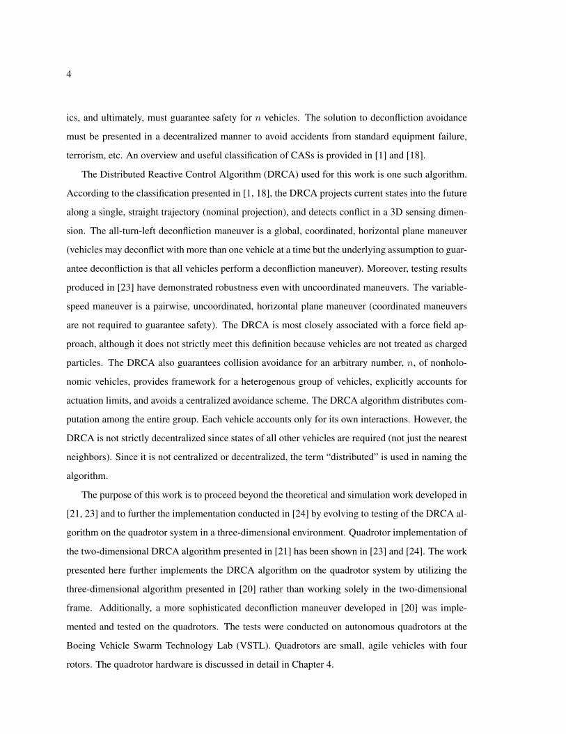
FAA divides the national airspace into regions called Air Route Traffic Control Centers (ARTCC).
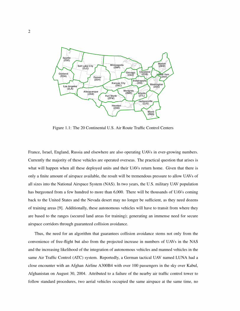
The 20 ARTCC for the continental U.S. are shown in Figure 1. Each region is further divided into
sectors, which are assigned to controllers who are responsible for conflict detection and resolution
within their sectors. To ensure that controller workload remains manageable, the number of flights
allowed in a sector at one time are constrained to a predetermined maximum value of 20 flights
[25]. Upstream controllers and air traffic managers delay and/or maneuver flights in order to en-
force these constraints. If using free-flight, aircraft would have more flexibility to follow efficient
routes in response to changing conditions. The loss of an airway structure however, would make
the process of detecting and resolving conflicts between aircraft much more complex and ultimately
would require a system where aircraft can avoid each other in a decentralized manner rather than
relying on a centralized system with a land-based controller.
The U.S. military alone operates thousands of autonomous vehicles. Further, militaries from
2
Figure 1.1: The 20 Continental U.S. Air Route Traffic Control Centers
France, Israel, England, Russia and elsewhere are also operating UAVs in ever-growing numbers.
Currently the majority of these vehicles are operated overseas. The practical question that arises is
what will happen when all these deployed units and their UAVs return home. Given that there is
only a finite amount of airspace available, the result will be tremendous pressure to allow UAVs of
all sizes into the National Airspace System (NAS). In two years, the U.S. military UAV population
has burgeoned from a few hundred to more than 6,000. There will be thousands of UAVs coming
back to the United States and the Nevada desert may no longer be sufficient, as they need dozens
of training areas [9]. Additionally, these autonomous vehicles will have to transit from where they
are based to the ranges (secured land areas for training); generating an immense need for secure
airspace corridors through guaranteed collision avoidance.
Thus, the need for an algorithm that guarantees collision avoidance stems not only from the
convenience of free-flight but also from the projected increase in numbers of UAVs in the NAS
and the increasing likelihood of the integration of autonomous vehicles and manned vehicles in the
same Air Traffic Control (ATC) system. Reportedly, a German tactical UAV named LUNA had a
close encounter with an Afghan Airline A300B4 with over 100 passengers in the sky over Kabul,
Afghanistan on August 30, 2004. Attributed to a failure of the nearby air traffic control tower to
follow standard procedures, two aerial vehicles occupied the same airspace at the same time, no
3
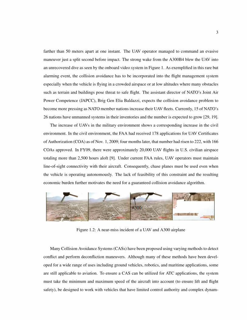
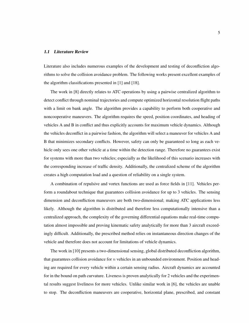
farther than 50 meters apart at one instant. The UAV operator managed to command an evasive
maneuver just a split second before impact. The strong wake from the A300B4 blew the UAV into
an unrecovered dive as seen by the onboard video system in Figure 1. As exemplified in this rare but
alarming event, the collision avoidance has to be incorporated into the flight management system
especially when the vehicle is flying in a crowded airspace or at low altitudes where many obstacles
such as terrain and buildings pose threat to safe flight. The assistant director of NATO’s Joint Air
Power Competence (JAPCC), Brig Gen Elia Baldazzi, expects the collision avoidance problem to
become more pressing as NATO member nations increase their UAV fleets. Currently, 15 of NATO’s
26 nations have unmanned systems in their inventories and the number is expected to grow [29, 19].
The increase of UAVs in the military environment shows a corresponding increase in the civil
environment. In the civil environment, the FAA had received 178 applications for UAV Certificates
of Authorization (COA) as of Nov. 1, 2009; four months later, that number had risen to 222, with 166
COAs approved. In FY09, there were approximately 20,000 UAV flights in U.S. civilian airspace
totaling more than 2,500 hours aloft [9]. Under current FAA rules, UAV operators must maintain
line-of-sight connectivity with their aircraft. Consequently, chase planes must be used even when
the vehicle is operating autonomously. The lack of feasibility of this constraint and the resulting
economic burden further motivates the need for a guaranteed collision avoidance algorithm.
Figure 1.2: A near-miss incident of a UAV and A300 airplane
Many Collision Avoidance Systems (CASs) have been proposed using varying methods to detect
conflict and perform deconfliction maneuvers. Although many of these methods have been devel-
oped for a wide range of uses including ground vehicles, robotics, and maritime applications, some
are still applicable to aviation. To ensure a CAS can be utilized for ATC applications, the system
must take the minimum and maximum speed of the aircraft into account (to ensure lift and flight
safety), be designed to work with vehicles that have limited control authority and complex dynam-
4
ics, and ultimately, must guarantee safety for n vehicles. The solution to deconfliction avoidance
must be presented in a decentralized manner to avoid accidents from standard equipment failure,
terrorism, etc. An overview and useful classification of CASs is provided in [1] and [18].
The Distributed Reactive Control Algorithm (DRCA) used for this work is one such algorithm.
According to the classification presented in [1, 18], the DRCA projects current states into the future
along a single, straight trajectory (nominal projection), and detects conflict in a 3D sensing dimen-
sion. The all-turn-left deconfliction maneuver is a global, coordinated, horizontal plane maneuver
(vehicles may deconflict with more than one vehicle at a time but the underlying assumption to guar-
antee deconfliction is that all vehicles perform a deconfliction maneuver). Moreover, testing results
produced in [23] have demonstrated robustness even with uncoordinated maneuvers. The variable-
speed maneuver is a pairwise, uncoordinated, horizontal plane maneuver (coordinated maneuvers
are not required to guarantee safety). The DRCA is most closely associated with a force field ap-
proach, although it does not strictly meet this definition because vehicles are not treated as charged
particles. The DRCA also guarantees collision avoidance for an arbitrary number, n, of nonholo-
nomic vehicles, provides framework for a heterogenous group of vehicles, explicitly accounts for
actuation limits, and avoids a centralized avoidance scheme. The DRCA algorithm distributes com-
putation among the entire group. Each vehicle accounts only for its own interactions. However, the
DRCA is not strictly decentralized since states of all other vehicles are required (not just the nearest
neighbors). Since it is not centralized or decentralized, the term “distributed” is used in naming the
algorithm.
The purpose of this work is to proceed beyond the theoretical and simulation work developed in
[21, 23] and to further the implementation conducted in [24] by evolving to testing of the DRCA al-
gorithm on the quadrotor system in a three-dimensional environment. Quadrotor implementation of
the two-dimensional DRCA algorithm presented in [21] has been shown in [23] and [24]. The work
presented here further implements the DRCA algorithm on the quadrotor system by utilizing the
three-dimensional algorithm presented in [20] rather than working solely in the two-dimensional
frame. Additionally, a more sophisticated deconfliction maneuver developed in [20] was imple-
mented and tested on the quadrotors. The tests were conducted on autonomous quadrotors at the
Boeing Vehicle Swarm Technology Lab (VSTL). Quadrotors are small, agile vehicles with four
rotors. The quadrotor hardware is discussed in detail in Chapter 4.
5
1.1 Literature Review
Literature also includes numerous examples of the development and testing of deconfliction algo-
rithms to solve the collision avoidance problem. The following works present excellent examples of
the algorithm classifications presented in [1] and [18].
The work in [8] directly relates to ATC operations by using a pairwise centralized algorithm to
detect conflict through nominal trajectories and compute optimized horizontal resolution flight paths
with a limit on bank angle. The algorithm provides a capability to perform both cooperative and
noncooperative maneuvers. The algorithm requires the speed, position coordinates, and heading of
vehicles A and B in conflict and thus explicitly accounts for maximum vehicle dynamics. Although
the vehicles deconflict in a pairwise fashion, the algorithm will select a maneuver for vehicles A and
B that minimizes secondary conflicts. However, safety can only be guaranteed so long as each ve-
hicle only sees one other vehicle at a time within the detection range. Therefore no guarantees exist
for systems with more than two vehicles; especially as the likelihood of this scenario increases with
the corresponding increase of traffic density. Additionally, the centralized scheme of the algorithm
creates a high computation load and a question of reliability on a single system.
A combination of repulsive and vortex functions are used as force fields in [11]. Vehicles per-
form a roundabout technique that guarantees collision avoidance for up to 3 vehicles. The sensing
dimension and deconfliction maneuvers are both two-dimensional; making ATC applications less
likely. Although the algorithm is distributed and therefore less computationally intensive than a
centralized approach, the complexity of the governing differential equations make real-time compu-
tation almost impossible and proving kinematic safety analytically for more than 3 aircraft exceed-
ingly difficult. Additionally, the prescribed method relies on instantaneous direction changes of the
vehicle and therefore does not account for limitations of vehicle dynamics.
The work in [10] presents a two-dimensional sensing, global distributed deconfliction algorithm,
that guarantees collision avoidance for n vehicles in an unbounded environment. Position and head-
ing are required for every vehicle within a certain sensing radius. Aircraft dynamics are accounted
for in the bound on path curvature. Liveness is proven analytically for 2 vehicles and the experimen-
tal results suggest liveliness for more vehicles. Unlike similar work in [6], the vehicles are unable
to stop. The deconfliction maneuvers are cooperative, horizontal plane, prescribed, and constant
6
speed. The prescribed cooperative maneuvers present a problem in that in real-life scenarios it may
be necessary to adapt the resolution maneuver to account for unexpected events in the environment.
Therefore, the algorithm is not robust to failed communications, etc.
A biologically inspired two-dimensional decentralized algorithm, but perhaps still applicable to
ATC scenarios, is presented in [15]. Instead of the traditional potential based function that repels a
vehicle in a particular direction, the algorithm only indicates to the vehicle where it should not go;
a similar technique to the maneuvering of a bat [18]. The desirability of directions are influenced by
the vehicle’s goal direction, actuation limits, and vehicle dynamics. The areas in which the vehicle
should not go are ranked according to the signal of the sonar response which includes distance to
the obstacle and the size of the obstacle. A winner-take-all method is used to guide steering. The
algorithm is unusual in that it combines both a method for sensing (rather than communicating)
as well as deconfliction detection and maneuvers. However, the algorithm has only been tested on
stationary obstacles and has no guarantee of collision avoidance.
This thesis is organized as follows. The quadrotor model is described in Chapter 2. The the-
oretical work developed by Lalish in [21],[22],[20] is introduced in Chapter 3. The Boeing VSTL
testbed and Boeing-developed simulation environment is described in Chapter 4. Two and three-
dimensional flight tests and simulations are presented in Chapter 5 using the all-turn-left deconflic-
tion maneuver. Chapter 6 describes the two and three-dimensional simulations utilizing a variable-
speed deconfliction maneuver. Finally, concluding remarks and possible future work are presented
in Chapter 7.
7
Chapter 2
QUADROTOR SYSTEM
The work here presents implementation of a three-dimensional method for deconflicting n vehi-
cles on a quadrotor system. Previous work has demonstrated that the algorithm can be implemented
on a variety of systems [20]. Therefore, the system model here can be applied to varying vehicle
types other than quadrotors. An arbitrary outer-loop controller provides each vehicle with a nominal
desired control input, ud(t). The controller is designed for the vehicle to execute any desired task.
These tasks may encompass target tracking, waypoint navigation, area searching, etc. The controller
determines a desired control input which is then output as a velocity vector and passed to the DRCA
algorithm. The DRCA algorithm then provides a modified control to guarantee collision avoidance
which is fed back to the outer-loop controller as a velocity. While the primary goal of the DRCA
algorithm is to prevent collisions, a similarly important goal is to allow assigned tasks to still be
performed in an efficient manner. This can be accomplished by minimizing the adjustment in the
control input in order to stay close to the desired control input (keeping in mind that this desired
control can change with time). The variable-speed maneuver presented in Chapter 6 is one such
method where the minimum control input is used to avoid a collision.
The notation throughout this paper will use bold face for vectors, hats over unit-vectors, script
capital letters for sets, standard capital letters for matrices and functions, and everything else is
assumed scalar. Quantities subscripted with t, n, or b refer to the tangent, normal, or binormal
direction, respectively.
The DRCA’s approach to collision avoidance only requires the position and velocity states of
the vehicles. Orientations can affect performance of vehicles, as they often have bearing on the
magnitude of acceleration available in a particular direction, but they do not directly affect the
underlying features of conflict and collision. In this way, many different vehicle models can work
equivalently with this approach. However, because of the quadrotor’s symmetry, the orientation does
not directly affect the dynamics (r and v), and as such can be arbitrary. Therefore, the quadrotor
8
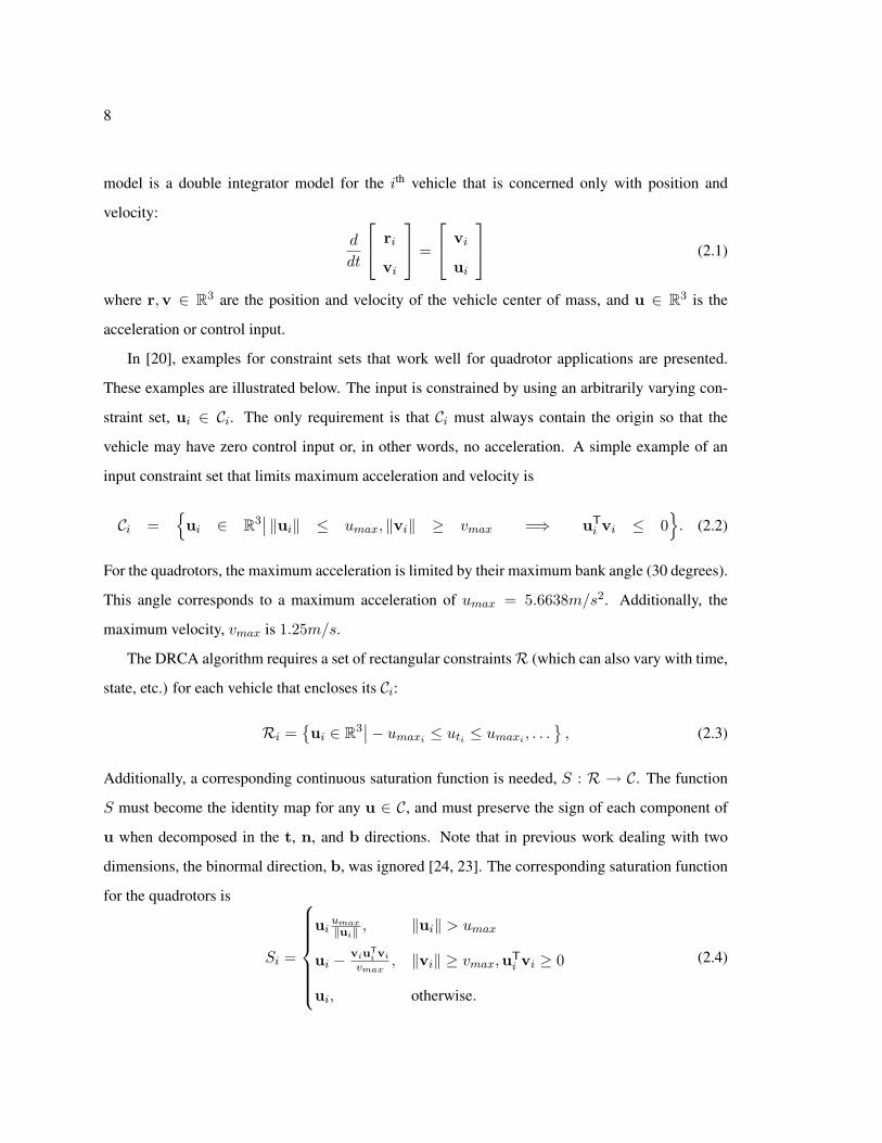
model is a double integrator model for the ith vehicle that is concerned only with position and
velocity:
d
dt
ri
vi
=
vi
ui
(2.1)
where r,v ∈ R3 are the position and velocity of the vehicle center of mass, and u ∈ R3 is the
acceleration or control input.
In [20], examples for constraint sets that work well for quadrotor applications are presented.
These examples are illustrated below. The input is constrained by using an arbitrarily varying con-
straint set, ui ∈ Ci. The only requirement is that Ci must always contain the origin so that the
vehicle may have zero control input or, in other words, no acceleration. A simple example of an
input constraint set that limits maximum acceleration and velocity is
Ci ={ui ∈ R3
∣∣ ‖ui‖ ≤ umax, ‖vi‖ ≥ vmax =⇒ uTi vi ≤ 0
}. (2.2)
For the quadrotors, the maximum acceleration is limited by their maximum bank angle (30 degrees).
This angle corresponds to a maximum acceleration of umax = 5.6638m/s2. Additionally, the
maximum velocity, vmax is 1.25m/s.
The DRCA algorithm requires a set of rectangular constraintsR (which can also vary with time,
state, etc.) for each vehicle that encloses its Ci:
Ri ={ui ∈ R3
∣∣− umaxi ≤ uti ≤ umaxi , . . .} , (2.3)
Additionally, a corresponding continuous saturation function is needed, S : R → C. The function
S must become the identity map for any u ∈ C, and must preserve the sign of each component of
u when decomposed in the t, n, and b directions. Note that in previous work dealing with two
dimensions, the binormal direction, b, was ignored [24, 23]. The corresponding saturation function
for the quadrotors is
Si =
ui umax‖ui‖ , ‖ui‖ > umax
ui −viu
Ti vi
vmax, ‖vi‖ ≥ vmax,uT
i vi ≥ 0
ui, otherwise.
(2.4)
9
Chapter 3
DRCA THEORETICAL WORK
3.1 Collision Cone and Conflict Detection
The quadrotors considered here are modeled as point masses, however these physical vehicles have
finite size. Therefore, to account for physical constraints in the theoretical model, the condition for
conflict is not to attain the same position in space at the same time, but rather to come within a
minimum allowed distance of each other at some point in time. For the quadrotors, this distance is
the approximate sum of the radii for two vehicles, dsep = 1 m. For other purposes, this minimum
distance could be, for example, the five nautical mile separation between aircraft required by the
FAA.
Two fundamental concepts for collision avoidance are collision and conflict. These terms are
defined below and are also provided in [20]. The relative position vector from vehicle i to vehicle
j is denoted rij ≡ rj − ri, while the relative velocity vector is defined in the opposite sense:
vij ≡ vi − vj . These definitions imply that ˙rij = −vij , and ˙vij = ui − uj . Note that this work
now includes the binormal component, b, of the velocity and position and will therefore result in a
three-dimensional collision cone rather than a two-dimensional cone as referenced in [23].
Definition 1 (Collision) A collision occurs between vehicles i and j when
‖rij‖ < dsep,ij ,
where dsep,ij is the minimum allowed separation distance between the vehicles’ geometric centers.
This distance can be different for any pair of vehicles to allow for heterogeneity of the system.
For two vehicles not already in a collision, the next question is whether they will collide if they
remain on their current trajectory. This situation will be called a conflict.
Definition 2 (Conflict) A conflict occurs between vehicles i and j if they are not currently in a
collision, but with zero control input (i.e. zero acceleration / constant velocity), at some future point
10
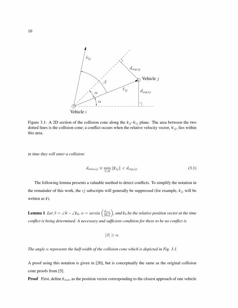
Vehicle i
Vehicle jβ
α
α
vij
dsep,ij
dsep,ijrij
Figure 3.1: A 2D section of the collision cone along the rij-vij plane. The area between the twodotted lines is the collision cone; a conflict occurs when the relative velocity vector, vij , lies withinthis area.
in time they will enter a collision:
dmin,ij ≡ mint>0‖rij‖ < dsep,ij . (3.1)
The following lemma presents a valuable method to detect conflicts. To simplify the notation in
the remainder of this work, the ij subscripts will generally be suppressed (for example, rij will be
written as r).
Lemma 1 Let β = ∠v−∠r0, α = arcsin(dsep‖r0‖
), and r0 be the relative position vector at the time
conflict is being determined. A necessary and sufficient condition for there to be no conflict is
|β| ≥ α.
The angle α represents the half-width of the collision cone which is depicted in Fig. 3.1.
A proof using this notation is given in [20], but is conceptually the same as the original collision
cone proofs from [5].
Proof First, define rmin as the position vector corresponding to the closest approach of one vehicle
11
to another in (3.1). By definition, at rmin the time derivative of ‖r‖2 = 0. Therefore:
d
dt
(rTr)
= 0
vTrmin = 0. (3.2)
Next, note that for constant velocity, v:
rmin = r0 − vt, (3.3)
where t is the time to closest approach. To find t, multiply by vT on both sides of (3.3), apply (3.2)
and solve:
vTrmin = vTr0 − vTvt
0 = ‖v‖ ‖r0‖ cosβ − ‖v‖2 t
t =‖r0‖‖v‖
cosβ. (3.4)
Now, using (3.2), (3.3) and (3.4), a concise expression for the closest approach distance is given by
dmin =√
rTminrmin
=√
(r0 − vt)Trmin
=√
rT0 (r0 − vt)
=
√‖r0‖2 − ‖v‖ ‖r0‖ cosβ
(‖r0‖‖v‖
cosβ)
=√‖r0‖2 (1− cos2 β)
= ‖r0‖ |sinβ| . (3.5)
For no conflict to occur, the converse of (3.1) must be true:
dsep ≤ dmin
= ‖r0‖ |sinβ| . (3.6)
Therefore, to remain free of conflict it is necessary that:
|β| ≥ arcsin(dsep‖r0‖
)= α. (3.7)
12
Separated?Desired
Control
Deconfliction
Maintenance
Deconfliction
Maneuver
Enter
Conflict−Free?
No
Yes
Yes
No
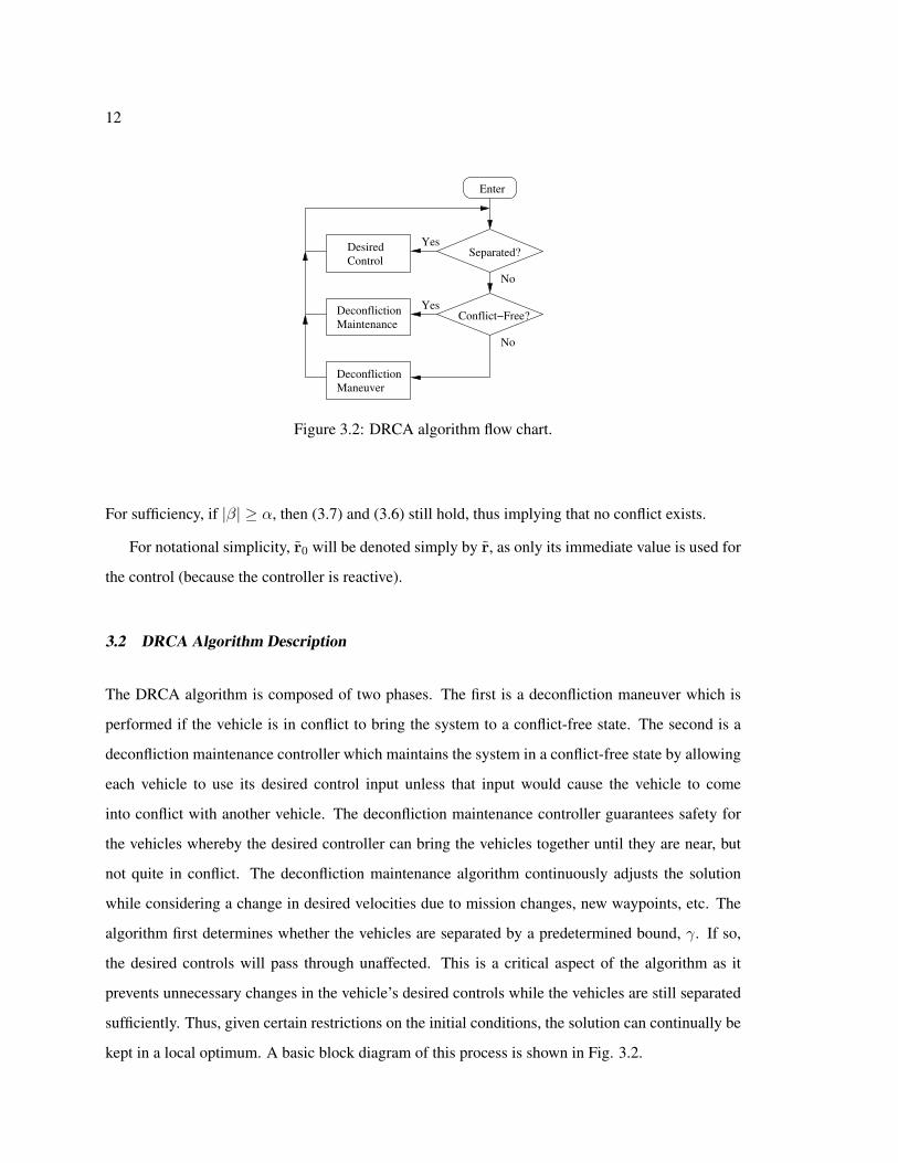
Figure 3.2: DRCA algorithm flow chart.
For sufficiency, if |β| ≥ α, then (3.7) and (3.6) still hold, thus implying that no conflict exists.
For notational simplicity, r0 will be denoted simply by r, as only its immediate value is used for
the control (because the controller is reactive).
3.2 DRCA Algorithm Description
The DRCA algorithm is composed of two phases. The first is a deconfliction maneuver which is
performed if the vehicle is in conflict to bring the system to a conflict-free state. The second is a
deconfliction maintenance controller which maintains the system in a conflict-free state by allowing
each vehicle to use its desired control input unless that input would cause the vehicle to come
into conflict with another vehicle. The deconfliction maintenance controller guarantees safety for
the vehicles whereby the desired controller can bring the vehicles together until they are near, but
not quite in conflict. The deconfliction maintenance algorithm continuously adjusts the solution
while considering a change in desired velocities due to mission changes, new waypoints, etc. The
algorithm first determines whether the vehicles are separated by a predetermined bound, γ. If so,
the desired controls will pass through unaffected. This is a critical aspect of the algorithm as it
prevents unnecessary changes in the vehicle’s desired controls while the vehicles are still separated
sufficiently. Thus, given certain restrictions on the initial conditions, the solution can continually be
kept in a local optimum. A basic block diagram of this process is shown in Fig. 3.2.
13
3.3 Deconfliction Maneuver
A deconfliction maneuver must involve some sort of acceleration change, which means either chang-
ing speed, altitude, or turning. In [1], the possible maneuvers are classified as horizontal plane (turn
left/right), vertical plane (climb/dive), and/or speedup and slowdown commands. These maneuvers
can be performed in combinations simultaneously or in sequence. Although the deconfliction al-
gorithm utilizes a three-dimensional collision cone, the deconfliction maneuvers utilized here are
essentially two-dimensional since the deconfliction maneuver does not modify the desired vertical
velocity. This method was chosen with the idea in mind that the majority of vehicles can modify a
heading easier rather than increasing the potential energy state. Additionally, since quadrotors are
limited by a maximum speed and can accelerate faster laterally, a turning approach in the horizontal
plane with speed changes is preferable. Thus, turning as a means of deconflicting is applicable to
both the quadrotors and a greater range of vehicles (necessary for future work).The most important
characteristic of a deconfliction maneuver is its ability to bring the vehicle to a conflict-free state
as quickly as possible with a guarantee that no collisions will occur during the maneuver (given
certain restrictions on the separation). A separation bound must be considered due to effects of lim-
ited control authority (a real vehicle is not capable of an instantaneous velocity in the conflict-free
direction).
Two deconfliction maneuvers will be presented here, first a simple all-turn-left maneuver that
nearly any vehicle is capable of, then a more sophisticated variable-speed maneuver that has better
performance at the cost of computational complexity. Both of these maneuvers are two-dimensional,
but conflict detection and deconfliction maintenance are conducted in 3D. In order to use these
maneuvers in a 3D application, the vehicle’s positions and velocities are projected onto the plane to
determine the deconfliction maneuver, then the original vertical component is added to the resulting
velocity. The guarantees of attaining a conflict-free state still apply (though the solutions are more
conservative) and once deconfliction maintenance takes over, the three-dimensional nature of the
system will be accounted for in a less conservative way. The variable-speed maneuver presented
here is more conservative in nature than the all-turn-left maneuver in that it assumes noncooperative
behavior for each maneuver.
14
3.3.1 All-turn-left Maneuver
One simple way to implement a turning approach is to have all vehicles in the conflict turn a specified
direction (either all left or all right) at a maximum rate until a conflict-free state is reached. The
specified maneuver allows for vehicles to deconflict in a global, rather than pairwise fashion. As
the name implies, vehicles in conflict turn left at maximum rate to get out of conflict. This basic
maneuver serves to demonstrate the 3D algorithm on the quadrotors, although a more sophisticated
and efficient deconfliction maneuver will be shown as well from work developed and proven in [20].
The all-turn-left deconfliction maneuver is defined by
ui = Lvi (3.8)
L =
0 −1 0
1 0 0
0 0 1
.In [21] it is proven that even when the system cannot reach a conflict-free state, the all-turn-
left coordinated maneuver simply becomes a loiter pattern. The underlying assumptions for this
proof are the existence of free space (the absence of nearby walls), a cooperative maneuver, and the
initialization of vehicles outside of conflict or in some cases, the predetermined bound. Simulation
computation scales to O(n) calculations and is insignificant when implemented on actual hardware
with n processors where each vehicle performs its own deconfliction maneuver.
Theorem 1 [20] If the initial separation of vehicles in an n-vehicle system satisfies
‖r‖ ≥ 2si
uni,max+ 2
sjunj,max
+ dsepij , (3.9)
where s is the vehicle’s speed, then all vehicles will remain collision free for all time if each vehicle
constantly turns at its maximum rate while maintaining constant speed.
Proof The trajectory each vehicle follows using constant turning is a circle of radius siuni,max
. As
long as a pair of vehicles is separated by at least the sum of the diameters of their loiter patterns and
the minimum separation distance, then they can never collide. Thus, this deconfliction maneuver
does guarantee safety for most cases.
15
3.3.2 Variable-Speed Maneuver
The quadrotors have no minimum speed (i.e. they can stop and hover), and they are capable of accel-
eration. The variable-speed maneuver takes advantage of these design characteristics although the
cost of this optimality is higher computational load. The all-turn-left maneuver did not take the head-
ing/orientation difference between vehicles into account when computing the necessary deconflic-
tion maneuver and assumed cooperative maneuvers while doing so. In contrast, the variable-speed
maneuver does not assume cooperative maneuvers to guarantee safety and gives a deconfliction ma-
neuver derived directly from the relative orientation of the vehicles in conflict. As results will show,
the variable-speed maneuver allows for more complicated collision schemes and facilitates the use
of minimum control input to avoid a collision–thereby allowing the vehicles to remain closer to their
desired velocities.
The allowable space for v′i is a disk, centered at the origin, of radius vi,max. The optimal solution
must either be a vertex between two collision cones, the nearest point on a single collision cone, or
the vertex between one collision cone and the edge of the allowable space. For the purposes of this
work, only the nearest point on a single collision cone and the vertex between one collision cone
and the edge of an allowable space are computed as allowable velocity vectors. This was done to
reduce computation time and to implement the algorithm in steps so that each part could be verified
to work correctly. Future work will show the full implementation of the variable-speed maneuver
provided in [20].
The first step of the algorithm is to compute the 2D unit-vector c for each side, representing the
direction of the edge of the collision cone (see Figure 3.1):
c = R(±α)r‖r‖
, (3.10)
where R is the 2× 2 rotation matrix.
Next, each of the nearest points on each collision cone (there is a right and a left solution for
each cone) are found, which is v′i = ccTv + vj . This list of points is checked to make sure each
‖v′i‖ ≤ vi,max. If this is not the case, then v′i is replaced with
v′i = vj − ccTvj ± c√
(cTvj)2 − vTj vj + v2
i,max. (3.11)
These points account for the only possible optima on the intersection of a cone and the edge of the
16
space. All of these points are ordered by increasing ∆vi and checked consecutively for conflicts
with the other vehicles. Because of the ordering, as soon as a point is found which is conflict free
for all j, it is the optimal solution and the algorithm terminates. In the case where no optimum
solution is found, the vehicle stops and hovers until the movement of the other vehicles causes a
solution to exist. Note that only one vehicle is allowed to stop at any given time. This variable-
speed maneuver greatly differs from other work such as [8] that was discussed previously because
although the computations are done in a pairwise manner, every solution is checked for conflicts
with the other n− 2 vehicles.
The optimization has a bound on its computation time since there are still a finite number of
possible optima to check. There are 2(n − 1) points to check for the nearest velocity vector on
each collision cone for each vehicle. There are an additional 4(n − 1) points to check for the
possible optima on the intersection of a cone and the edge of the space. Since these still need to be
checked for conflict with the other n − 2 collision cones, the maximum computation time is now
upper-bounded by cn2, where c is related to the time each type of computation requires.
Because the points are ordered by increasing ∆vi and the algorithm terminates as soon as viable
velocity vector is found, this algorithm usually terminates far before its maximum computation time.
This analysis would guarantee a conflict-free solution if the vehicle could attain its desired veloc-
ity vector instantaneously. However, the limited control authority available makes this impossible.
Instead, it takes a finite amount of time for the vehicle to attain its desired velocity, and during that
time it and the other vehicles move, which causes the collision cones to move. In order to ensure
that the system is still conflict-free after this motion, the initial collision cones must be enlarged to
the point of enclosing all possible movements.
To bound the collision cone, one must simply bound ‖∆r‖ ≤ δ, or how much the vehicles can
change position before the maneuver is complete. Then the width of the collision cone is enlarged
from (3.7) to
αe = arcsin(dsep + δ
‖r‖
). (3.12)
Note that this expression implies an initial separation of ‖r‖ ≥ dsep+δ, or else αe will be undefined.
Lemma 2 Let there be two vehicles (i and j), each modeled by a planar version of (2.1). Vehicle
j is subject to the maximum speed constraint ‖vj‖ ≤ vj,max. Vehicle i is subject to ‖ui‖ ≤ ui,max
17
and ‖vi‖ ≤ vi,max and is accelerating as quickly as possible from its initial velocity, vi, to its
desired velocity, v′i. The relative motion between the vehicles in the time it takes vehicle i to attain
its desired velocity is bounded by ‖∆r‖ ≤ δ, where
δ =vi,maxui,max
(vi,max + 2vj,max) . (3.13)
Proof Let the angle between vi and v′i be 2γ and let t be the time required for the maneuver.
Then ‖∆vi‖ = ui,maxt, ‖∆ri‖ = t ‖vi + v′i‖ /2, and ‖∆rj‖ ≤ vj,maxt. Also, ‖vi + v′i‖ ≤
2vi,max cos γ and ‖∆vi‖ ≤ 2vi,max |sin γ|. Therefore,
‖∆r‖ ≤ ‖∆ri‖+ ‖∆rj‖ ≤2v2i,max |cos γ sin γ|
ui,max+
2vi,maxvj,max |sin γ|ui,max
≤ vi,maxui,max
(vi,max + 2vj,max) . (3.14)
This bound can in turn be used in (3.12) to size the enlarged collision cone. The following
theorem states how this bound can be used to keep vehicles from colliding during a deconfliction
maneuver.
Theorem 2 [20] Let there be a set of vehicles, D, which are not in conflict with each other. When
another vehicle, i, is in conflict with some or all members of D and performs the variable-speed
maneuver, the system will be conflict-free in time t, where
t ≤ 2vi,maxui,max
, (3.15)
and no vehicles will collide during the maneuver. The vehicles are all modeled by a planar version
of (2.1), have speed constraints ‖vj‖ ≤ vj,max and vehicle i has the input constraint ‖ui‖ ≤ ui,max.
It is assumed that a feasible solution to the optimization problem, v′i, exists and that the vehicles in
D maintain a conflict-free state with v′i, using a cone with width defined by (3.12) and (3.13).
Proof If a feasible point exists for the optimization problem, then the optimal solution is guaranteed
to be found and this point will satisfy∣∣∠v′ − ∠r∣∣ ≥ arcsin
(dsep + δ
‖r‖
). (3.16)
The maximum amount of time required for vehicle i to get from its initial vi to v′i is
t = vi,maxui,max (vi,max + 2vj,max) , (3.17)
18
and during this time ∆r ≤ δ from Lemma 2. Therefore, once the desired velocities have been
attained, one still has ∣∣∠v′ − ∠(r + ∆r)∣∣ ≥ arcsin
(dsep‖r‖
), (3.18)
meaning the vehicles are not in conflict. The vehicles cannot collide during this time because as
stated earlier, the pairs must be initially separated by at least ‖r‖ ≥ dsep + δ, which means after the
maneuver, they still must be outside of collision because ‖r + ∆r‖ ≥ dsep. Of course, the theorem
above does not hold if a feasible solution does not exist for the optimization. The following theorem
gives a conditional bound, χi(D), on initial separation that is sufficient to guarantee the existence of
a solution. Note that this conditional bound is based on the assumption that intersections of collision
cones are viable options as well. Additionally, noncooperative maneuvers are assumed. However, it
still serves as a good approximation for when n is small.
Theorem 3 [20] For vehicle i of an n-vehicle system in the plane, let vehicle i’s speed be con-
strained by ‖vi‖ ≤ vi,max, while each other vehicle’s speed is constrained by the uniform bound
‖vj‖ ≤ vmax. There exists an admissible velocity vector, v′i, which is conflict-free with the other
n− 1 vehicles, given that vehicle i is separated from the other vehicles such that
∑j∈D
αe ≤
arcsin
(vi,maxvmax
), vi,max < vmax
vi,maxui,max
(vi,max + 2vj,max) .(3.19)
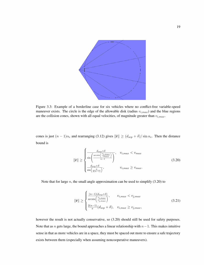
Proof In order for a conflict-free point to exist, the collision cones from the other vehicles cannot
completely cover the admissible disk of possible velocities of vehicle i. The worst case for this
coverage when the other vehicles are capable of higher speed than vehicle i is when all the vehicles
have the same velocity, with their maximum speed, and their positions splay out their collision cones
so as to form one large, continuous cone (see Fig. 3.3). The interior angle of this large cone must
be less than 2 arcsin(vi,max/vmax) to ensure that it cannot cover the entire admissible circle. When
vehicle i’s speed is higher than the other vehicles, the arcsine takes on its limiting value of π/2
and becomes conservative because it only allows the combined collision cone to cover a half-space
within the disk. Together these constraints form (3.19).
In the special case where all of the vehicles are exactly the same distance away (as in Fig. 3.3),
the bound (3.19) can be simplified to a bound on distance. First note that the sum of the collision
19
Figure 3.3: Example of a borderline case for six vehicles where no conflict-free variable-speedmaneuver exists. The circle is the edge of the allowable disk (radius vi,max) and the blue regionsare the collision cones, shown with all equal velocities, of magnitude greater than vi,max.
cones is just (n − 1)αe and rearranging (3.12) gives ‖r‖ ≥ (dsep + δ)/ sinαe. Then the distance
bound is
‖r‖ ≥
dsep+δ
sin
arcsin
(vi,maxvmax
)n−1
, vi,max < vmax
dsep+δ
sin(
π2(n−1)
) , vi,max ≥ vmax.
(3.20)
Note that for large n, the small angle approximation can be used to simplify (3.20) to
‖r‖ ≥
(n−1)(dsep+δ)
arcsin
(vi,maxvj,max
) , vi,max < vj,max
2(n−1)π (dsep + δ), vi,max ≥ vj,max,
(3.21)
however the result is not actually conservative, so (3.20) should still be used for safety purposes.
Note that as n gets large, the bound approaches a linear relationship with n−1. This makes intuitive
sense in that as more vehicles are in a space, they must be spaced out more to ensure a safe trajectory
exists between them (especially when assuming noncooperative maneuvers).
20
c
dsep
dsep
vj
vi
e
r
pt,ijti
α
αβ
v
sipn,ijni
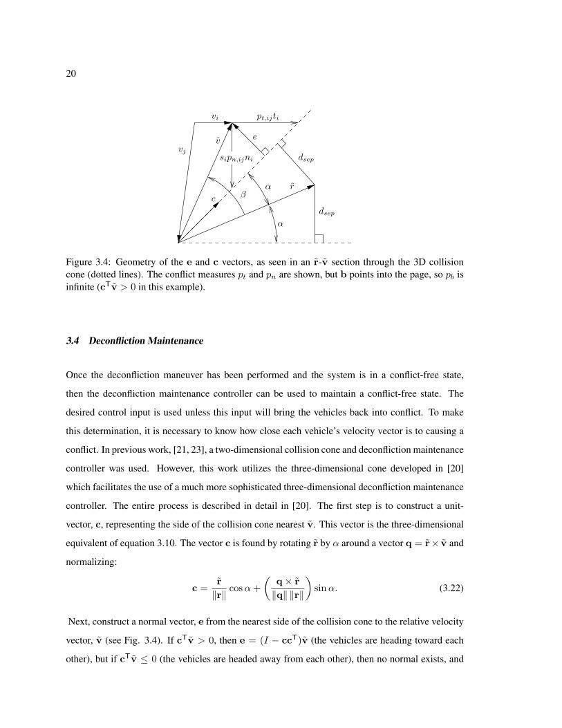
Figure 3.4: Geometry of the e and c vectors, as seen in an r-v section through the 3D collisioncone (dotted lines). The conflict measures pt and pn are shown, but b points into the page, so pb isinfinite (cTv > 0 in this example).
3.4 Deconfliction Maintenance
Once the deconfliction maneuver has been performed and the system is in a conflict-free state,
then the deconfliction maintenance controller can be used to maintain a conflict-free state. The
desired control input is used unless this input will bring the vehicles back into conflict. To make
this determination, it is necessary to know how close each vehicle’s velocity vector is to causing a
conflict. In previous work, [21, 23], a two-dimensional collision cone and deconfliction maintenance
controller was used. However, this work utilizes the three-dimensional cone developed in [20]
which facilitates the use of a much more sophisticated three-dimensional deconfliction maintenance
controller. The entire process is described in detail in [20]. The first step is to construct a unit-
vector, c, representing the side of the collision cone nearest v. This vector is the three-dimensional
equivalent of equation 3.10. The vector c is found by rotating r by α around a vector q = r× v and
normalizing:
c =r‖r‖
cosα+(
q× r‖q‖ ‖r‖
)sinα. (3.22)
Next, construct a normal vector, e from the nearest side of the collision cone to the relative velocity
vector, v (see Fig. 3.4). If cTv > 0, then e = (I − ccT)v (the vehicles are heading toward each
other), but if cTv ≤ 0 (the vehicles are headed away from each other), then no normal exists, and
21
the nearest point on the collision cone is the tip, so e = v. Therefore:
e =
v, cTv ≤ 0
(I − ccT)v, cTv > 0.(3.23)
The next step is to ascertain how much control (change in velocity) can be applied in each of
these directions before a conflict develops. A useful approach to combine the effects of multiple
collision cones is to decompose the system into three component directions and analyze those di-
rections separately. Therefore, the coordinate system is defined by the orthonormal vectors t, n,
and b. Because the quadrotors have no heading change and the vehicle orientation does not matter
to the algorithm, the body frame is also fixed to the inertial coordinate frame. For simplicity, a
conservative approach is taken whereby the signed distance is found from v to the tangent plane
enclosing the collision cone (defined by the normal vector e) in each of the t, n, and b directions.
These signed distances are
pt,ij =‖eij‖2
eTijti
, pn,ij =‖eij‖2
eTijni
, and pb,ij =‖eij‖2
eTijbi
,
which are described graphically in Fig. 3.4.
Now define εt, εn, εb > 0 as thresholds such that when |pt| > εt, the conflict is far enough away
that it can be ignored for the purposes of deconfliction maintenance (and likewise for pn and pb).
The n-vehicle deconfliction maintenance controller running on vehicle i computes pt, pn, and pb to
each of the other vehicles within the predetermined separation bound γ and then finds the closest
conflict in each direction, i.e.
p+ti
= minj{pt,ij > 0, εti}
p−ti = −maxj{pt,ij < 0,−εti} ,
(3.24)
and likewise for pn and pb. Note that by definition 0 < p± ≤ ε because deconfliction maintenance
cannot occur outside the ε threshold. To simplify notation, in any case where a relation holds in all
of the tangent, normal, and binormal directions, the subscript associated with ε will be suppressed.
The input is constructed using a function, F , such that in each direction u = F (p+, p−, ud)
(meaning the control choice does not produce a conflict-generating velocity). This control function
22
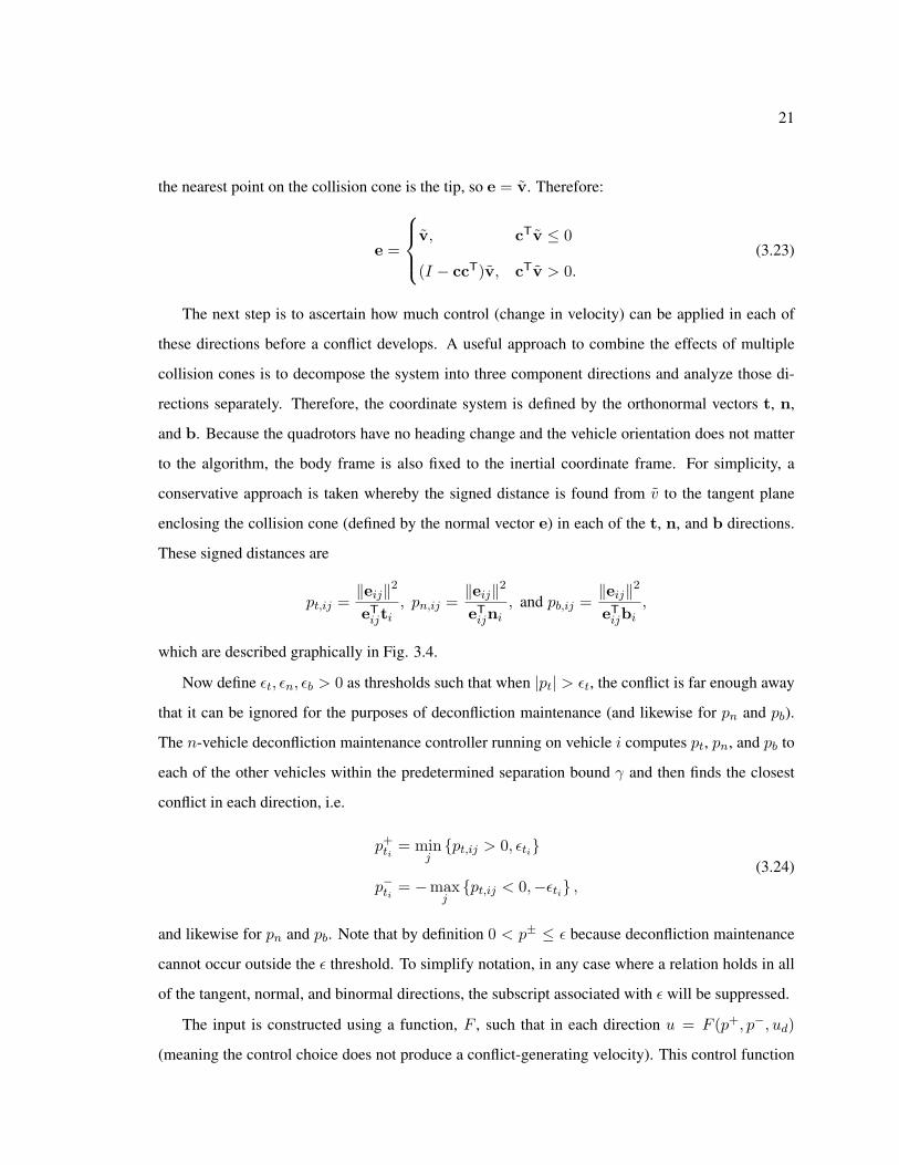
Figure 3.5: Example of the control function, F . Note that P4 increases and decreases with changingud.
is developed in [20]. The control function chosen for the implementation of the DRCA algorithm
here is
F (p+, p−, ud) =uminε
p+ +umaxε
p− +ud − umax − umin
ε2p+p−, (3.25)
because it is a bilinear interpolation of the following ordered triples of the form (p+, p−, u):
P1 = (0, 0, 0) P2 = (ε, 0, umin)
P3 = (0, ε, umax) P4 = (ε, ε, ud).
Note that when p+ = p− = ε, F (p+, p−) = ud. An example of this control function is shown in
Fig. 3.5. For F to function correctly, ud must be saturated such that
umin ≤ ud ≤ umax. (3.26)
This choice of control function means that once u is constructed from its three components, then
u ∈ R. Then the saturation function S will give the final resultant control vector, which will be in
C.
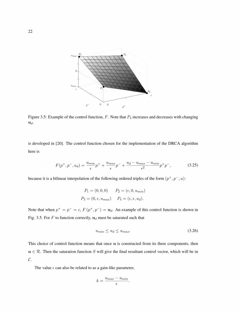
The value ε can also be related to as a gain-like parameter,
k =umax − umin
ε.
23
r~
sepd
sepd
Figure 3.6: Visual illustration of the spring-like buffer, ε. If a vehicle tries to push against this buffertowards a conflict, the buffer will push back. The faster a vehicle is accelerating toward the collisioncone, the harder the buffer will push back.
k can be considered as a spring constant and has units of inverse seconds. In this case, the threshold
ε can be considered as a spring-like buffer. Note that the magnitude of the gradient of the control
function will always be less than or equal to k, regardless of the desired control. An example of this
buffer is shown in Fig. 3.6.
Given that the deconfliction group,D, has n vehicles, this algorithm’s computation time on each
vehicle scales asO(n) because only the computation of the other vehicle’s collision cone is required.
The computed information then results in a control function. Although O(n2) computations happen
in the entire group, these computations are independent of each other (only linked by the sensed or
communicated states) and occur in parallel in a distributed fashion, so only the per-vehicle scaling
affects computation time. The system is guaranteed to maintain its conflict-free state for n vehicles
despite arbitrary control authority restrictions with the following theorem [20].
Each time a new vehicle enters bound and is added to the deconfliction group, D, the vehicle
immediately broadcasts a conflict-free velocity to the group. This conflict-free velocity is obtained
through the deconfliction maneuver phase and is broadcast even if the vehicle has not yet achieved
the deconfliction velocity. Since it is this broadcast velocity that is used by the deconfliction mainte-
nance algorithm until the new vehicle really is conflict-free, the deconfliction group never sees any
new conflicts.
Theorem 4 [20] The deconfliction maintenance controller described above, when implemented on
n vehicles with dynamics (2.1) and inputs constrained by Ci, will keep the system collision free for
all time if the system starts conflict-free.
24
Proof To measure the distance to a collision, define m as a signed version of ‖e‖ (in terms of v
from the geometry in Fig. 3.4):
m =
‖v‖ , cTv ≤ 0
‖v‖ sin(|β| − α), cTv > 0.(3.27)
Note that m is negative during conflict and positive during no conflict.
To ensure that a conflicted state is never reached (i.e. m is always greater than zero), it is
sufficient to show that for every pair of vehicles there is a neighborhood on the positive side of
m = 0 where m ≥ 0. This condition implies that as the boundary of a collision cone approaches, it
will either stop approaching or recede before a conflict is formed. The fact that this is a one-sided
neighborhood is important because m does not exist at m = 0 for the same reason that ddt ‖v‖ does
not exist at v = 0. However, if this condition is satisfied, then m > 0 for all time, ensuring that
m 6= 0.
For cTv ≤ 0 (using the ij notation again briefly for clarity),
m =eT ˙vm
= eT ˙v, (3.28)
where e = e‖e‖ . Expanding ui into its components yields ui = [utiti + unini + ubibi]. Next
substitute for vij in (3.28) to get
eTij
˙vij = uti eTijti + uni e
Tijni + ubi e
Tijbi − utj eT
ijtj − unj eTijnj − ubj e
Tijbj . (3.29)
Because of the symmetry of the problem eji = −eij , so
eTij
˙vij =uti eTijti + uni e
Tijni + ubi e
Tijbi + utj e
Tjitj + unj e
Tjinj + ubj e
Tjibj
=mij
(utipt,ij
+unipn,ij
+ubipb,ij
+utjpt,ji
+unjpn,ji
+ubjpb,ji
). (3.30)
For cTv > 0, the derivative of (3.27) becomes
m = sin(|β| − α)d ‖v‖dt
+ ‖v‖ cos(|β| − α)d
dt(|β| − α). (3.31)
The derivative exists because m > 0 implies ‖v‖ 6= 0, |β| ≥ α > 0, and ‖r‖ ≥ dsep > 0. From the
geometry,
d |β|dt
= sgn(β)(d∠vdt− d∠r
dt
)= sgn(β)
d∠vdt
+‖v‖‖r‖|sinβ| . (3.32)
25
The derivative of α is somewhat less straight-forward:
dα
dt=
d
dt
(arcsin
(dsep‖r‖
))
=d
dt
(dsep‖r‖
)(1−
(dsep‖r‖
)2)−1/2
=dsep ‖v‖ cosβ‖r‖2
‖r‖√‖r‖2 − d2
sep
=‖v‖‖r‖
cosβ tanα. (3.33)
Combining the above two terms gives
d
dt(|β| − α) =
‖v‖‖r‖
(|sinβ| − cosβ tanα) + sgn(β)d∠vdt
, (3.34)
which can be substituted into (3.31) to get
m = sin(|β| − α)d ‖v‖dt
+ cos(|β| − α) sgn(β) ‖v‖ d∠vdt
+ cos(|β| − α)‖v‖2
‖r‖(|sinβ| − cosβ tanα). (3.35)
To simplify the above, note that in the case of cTv > 0, the geometry of the vectors (Fig. 3.4) gives
eT ˙v = sin(|β| − α)d ‖v‖dt
+ cos(|β| − α) sgn(β) ‖v‖ d∠vdt
. (3.36)
Therefore (3.35) reduces to
m = eT ˙v + cos(|β| − α)‖v‖2
‖r‖(|sinβ| − cosβ tanα). (3.37)
This expression can be further simplified by recognizing that
m
‖v‖ cosα=
sin |β| cosα− sinα cos |β|cosα
= |sinβ| − cosβ tanα. (3.38)
Therefore
m = eT ˙v +m‖v‖ cos(|β| − α)‖r‖ cosα
. (3.39)
The second term is always positive because cTv > 0 implies that cos(|β| − α) > 0, and α ≤ π/2
by definition. Combining this result with (3.28) implies that
m ≥ eT ˙v (3.40)
26
for any value of cTv. Recalling (3.30),
mij ≥ mij
(utipt,ij
+unipn,ij
+ubipb,ij
+utjpt,ji
+unjpn,ji
+ubjpb,ji
). (3.41)
As long as the controller ensures that uti has the same sign as pt,ij , etc. then m ≥ 0 for that pair
of vehicles. Note that each vehicle will automatically cooperative in avoiding conflicts since each
vehicle calculates its control from its own point of view.
Combining this result with the definitions (3.24), any continuous control function that satisfies
limp+ti→0+
uti ≥ 0, limp−ti→0+
uti ≤ 0,
limp+ni→0+
uni ≥ 0, limp−ni→0+
uni ≤ 0,
limp+bi→0+
ubi ≥ 0, limp−bi→0+
ubi ≤ 0,
(3.42)
also ensures that there is a neighborhood on the positive side of m = 0 for which m ≥ 0, guaran-
teeing the system cannot enter a conflicted state.
The control function used in this implementation (3.25) satisfies (3.42), so the deconfliction
maintenance controller will cause the n-vehicle system to remain conflict-free for all time, assuming
it started that way.
Results will hold for arbitrary (even time varying) ud, umin and umax, so long as they satisfy
(3.26) and R contains the origin at every instant. The key for this saturation to work is that S
preserve u, such that (3.42) is still satisfied.
27
Chapter 4
TESTBED AND SIMULATION ENVIRONMENT
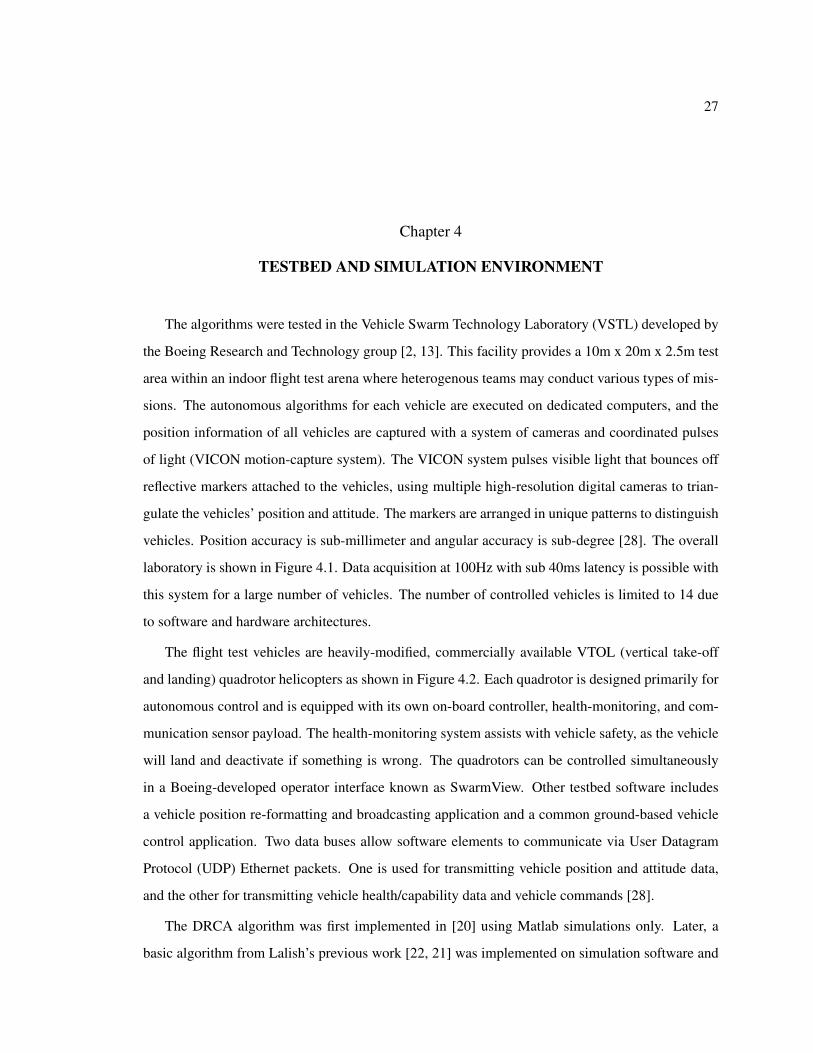
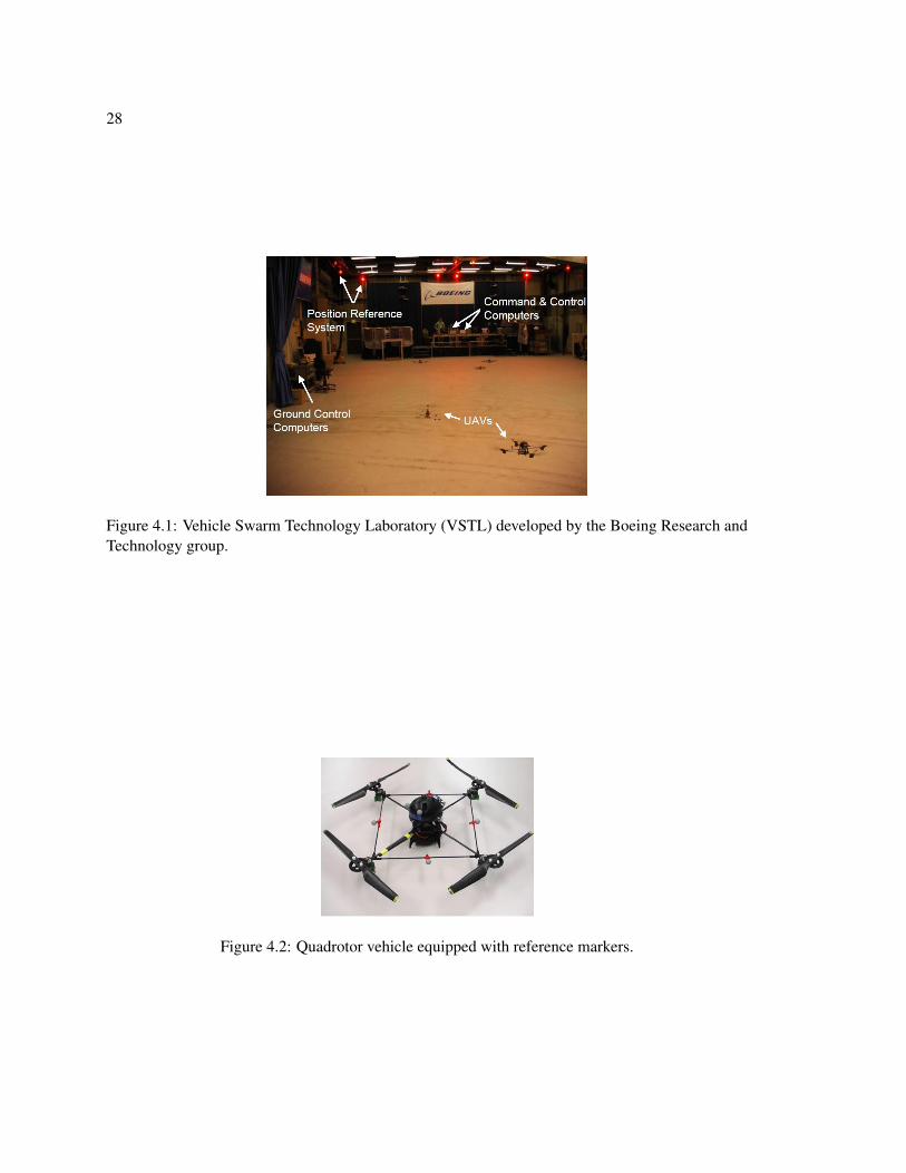
The algorithms were tested in the Vehicle Swarm Technology Laboratory (VSTL) developed by
the Boeing Research and Technology group [2, 13]. This facility provides a 10m x 20m x 2.5m test
area within an indoor flight test arena where heterogenous teams may conduct various types of mis-
sions. The autonomous algorithms for each vehicle are executed on dedicated computers, and the
position information of all vehicles are captured with a system of cameras and coordinated pulses
of light (VICON motion-capture system). The VICON system pulses visible light that bounces off
reflective markers attached to the vehicles, using multiple high-resolution digital cameras to trian-
gulate the vehicles’ position and attitude. The markers are arranged in unique patterns to distinguish
vehicles. Position accuracy is sub-millimeter and angular accuracy is sub-degree [28]. The overall
laboratory is shown in Figure 4.1. Data acquisition at 100Hz with sub 40ms latency is possible with
this system for a large number of vehicles. The number of controlled vehicles is limited to 14 due
to software and hardware architectures.
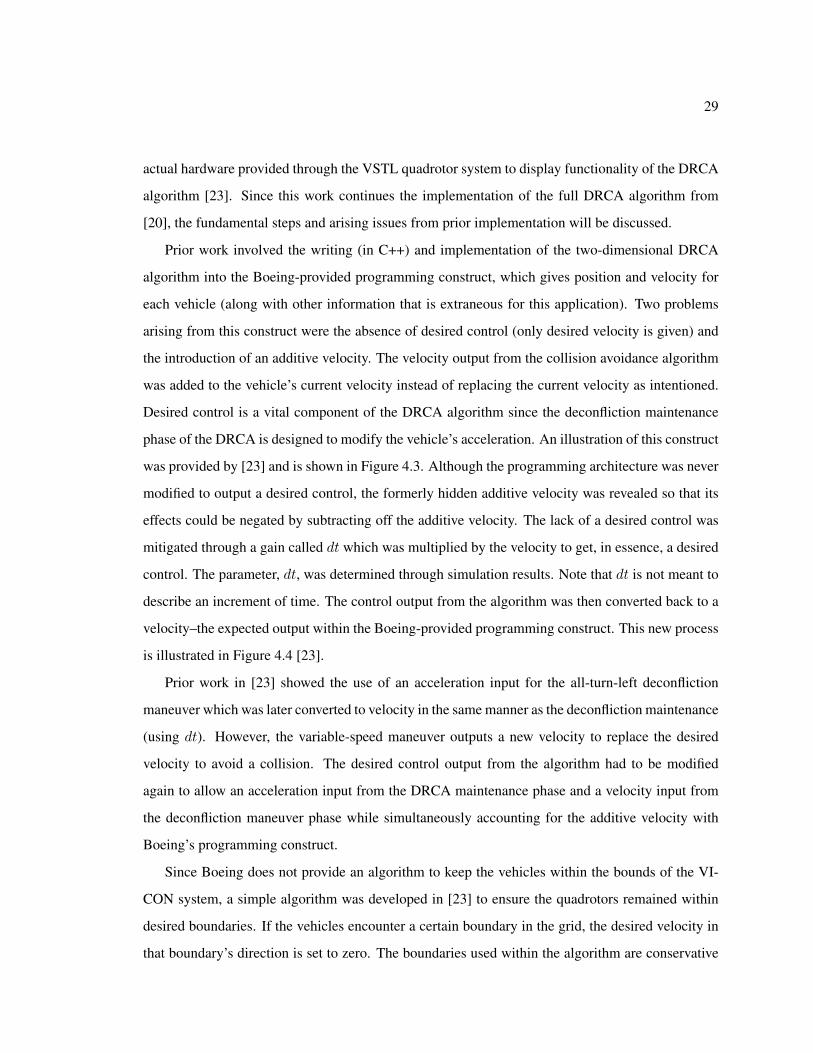
The flight test vehicles are heavily-modified, commercially available VTOL (vertical take-off
and landing) quadrotor helicopters as shown in Figure 4.2. Each quadrotor is designed primarily for
autonomous control and is equipped with its own on-board controller, health-monitoring, and com-
munication sensor payload. The health-monitoring system assists with vehicle safety, as the vehicle
will land and deactivate if something is wrong. The quadrotors can be controlled simultaneously
in a Boeing-developed operator interface known as SwarmView. Other testbed software includes
a vehicle position re-formatting and broadcasting application and a common ground-based vehicle
control application. Two data buses allow software elements to communicate via User Datagram
Protocol (UDP) Ethernet packets. One is used for transmitting vehicle position and attitude data,
and the other for transmitting vehicle health/capability data and vehicle commands [28].
The DRCA algorithm was first implemented in [20] using Matlab simulations only. Later, a
basic algorithm from Lalish’s previous work [22, 21] was implemented on simulation software and
28
Figure 4.1: Vehicle Swarm Technology Laboratory (VSTL) developed by the Boeing Research andTechnology group.
Figure 4.2: Quadrotor vehicle equipped with reference markers.
29
actual hardware provided through the VSTL quadrotor system to display functionality of the DRCA
algorithm [23]. Since this work continues the implementation of the full DRCA algorithm from
[20], the fundamental steps and arising issues from prior implementation will be discussed.
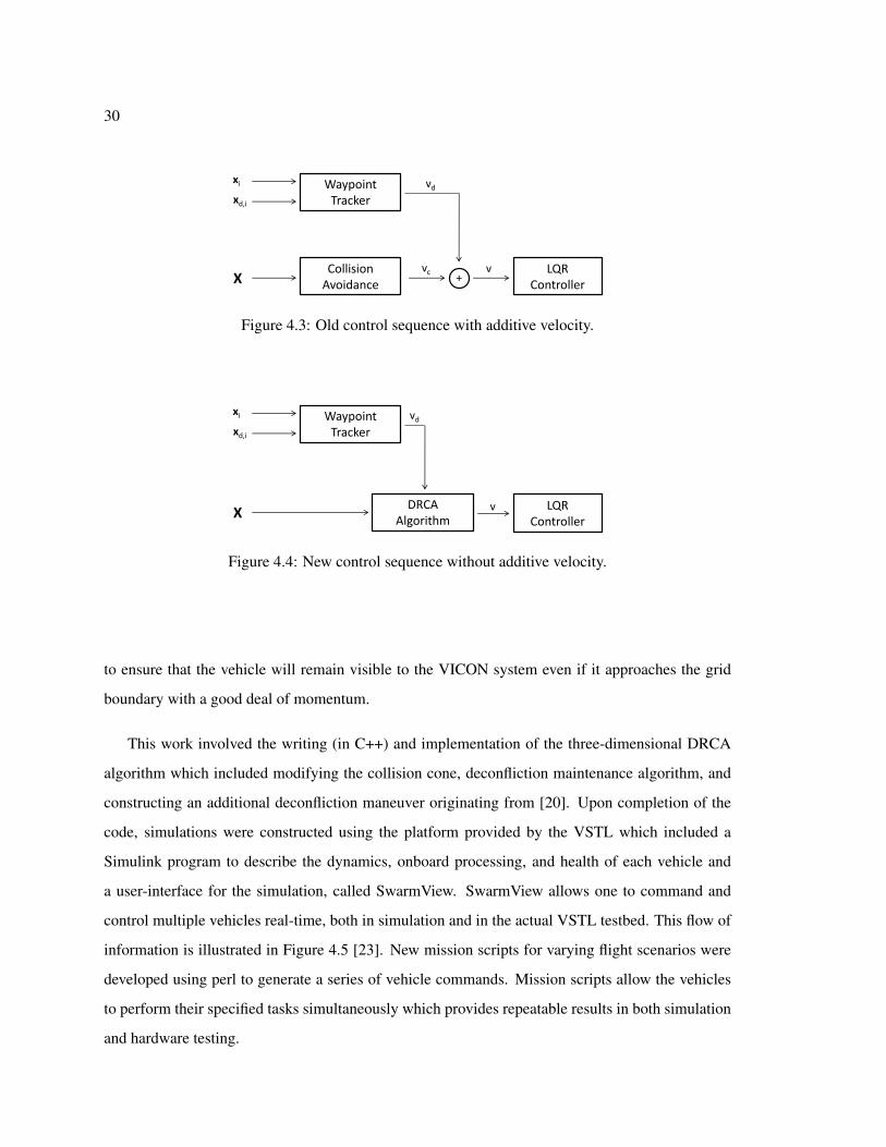
Prior work involved the writing (in C++) and implementation of the two-dimensional DRCA
algorithm into the Boeing-provided programming construct, which gives position and velocity for
each vehicle (along with other information that is extraneous for this application). Two problems
arising from this construct were the absence of desired control (only desired velocity is given) and
the introduction of an additive velocity. The velocity output from the collision avoidance algorithm
was added to the vehicle’s current velocity instead of replacing the current velocity as intentioned.
Desired control is a vital component of the DRCA algorithm since the deconfliction maintenance
phase of the DRCA is designed to modify the vehicle’s acceleration. An illustration of this construct
was provided by [23] and is shown in Figure 4.3. Although the programming architecture was never
modified to output a desired control, the formerly hidden additive velocity was revealed so that its
effects could be negated by subtracting off the additive velocity. The lack of a desired control was
mitigated through a gain called dt which was multiplied by the velocity to get, in essence, a desired
control. The parameter, dt, was determined through simulation results. Note that dt is not meant to
describe an increment of time. The control output from the algorithm was then converted back to a
velocity–the expected output within the Boeing-provided programming construct. This new process
is illustrated in Figure 4.4 [23].
Prior work in [23] showed the use of an acceleration input for the all-turn-left deconfliction
maneuver which was later converted to velocity in the same manner as the deconfliction maintenance
(using dt). However, the variable-speed maneuver outputs a new velocity to replace the desired
velocity to avoid a collision. The desired control output from the algorithm had to be modified
again to allow an acceleration input from the DRCA maintenance phase and a velocity input from
the deconfliction maneuver phase while simultaneously accounting for the additive velocity with
Boeing’s programming construct.
Since Boeing does not provide an algorithm to keep the vehicles within the bounds of the VI-
CON system, a simple algorithm was developed in [23] to ensure the quadrotors remained within
desired boundaries. If the vehicles encounter a certain boundary in the grid, the desired velocity in
that boundary’s direction is set to zero. The boundaries used within the algorithm are conservative
30
xi
xd,i
WaypointTracker
XCollisionAvoidance
LQRController
+
vd
vc v
Figure 4.3: Old control sequence with additive velocity.
xi
xd,i
WaypointTracker
XDRCA
AlgorithmLQR
Controller
vd
v
Figure 4.4: New control sequence without additive velocity.
to ensure that the vehicle will remain visible to the VICON system even if it approaches the grid
boundary with a good deal of momentum.
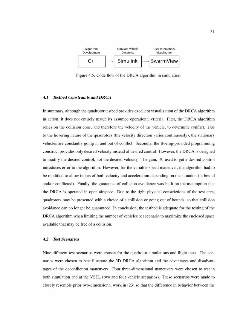
This work involved the writing (in C++) and implementation of the three-dimensional DRCA
algorithm which included modifying the collision cone, deconfliction maintenance algorithm, and
constructing an additional deconfliction maneuver originating from [20]. Upon completion of the
code, simulations were constructed using the platform provided by the VSTL which included a
Simulink program to describe the dynamics, onboard processing, and health of each vehicle and
a user-interface for the simulation, called SwarmView. SwarmView allows one to command and
control multiple vehicles real-time, both in simulation and in the actual VSTL testbed. This flow of
information is illustrated in Figure 4.5 [23]. New mission scripts for varying flight scenarios were
developed using perl to generate a series of vehicle commands. Mission scripts allow the vehicles
to perform their specified tasks simultaneously which provides repeatable results in both simulation
and hardware testing.
31
C++ Simulink SwarmView
Algorithm Development
Simulate Vehicle Dynamics
User Interaction/Visualization
Figure 4.5: Code flow of the DRCA algorithm in simulation.
4.1 Testbed Constraints and DRCA
In summary, although the quadrotor testbed provides excellent visualization of the DRCA algorithm
in action, it does not entirely match its assumed operational criteria. First, the DRCA algorithm
relies on the collision cone, and therefore the velocity of the vehicle, to determine conflict. Due
to the hovering nature of the quadrotors (the velocity direction varies continuously), the stationary
vehicles are constantly going in and out of conflict. Secondly, the Boeing-provided programming
construct provides only desired velocity instead of desired control. However, the DRCA is designed
to modify the desired control, not the desired velocity. The gain, dt, used to get a desired control
introduces error to the algorithm. However, for the variable-speed maneuver, the algorithm had to
be modified to allow inputs of both velocity and acceleration depending on the situation (in bound
and/or conflicted). Finally, the guarantee of collision avoidance was built on the assumption that
the DRCA is operated in open airspace. Due to the tight physical constrictions of the test area,
quadrotors may be presented with a choice of a collision or going out of bounds, so that collision
avoidance can no longer be guaranteed. In conclusion, the testbed is adequate for the testing of the
DRCA algorithm when limiting the number of vehicles per scenario to maximize the enclosed space
available that may be free of a collision.
4.2 Test Scenarios
Nine different test scenarios were chosen for the quadrotor simulations and flight tests. The sce-
narios were chosen to best illustrate the 3D DRCA algorithm and the advantages and disadvan-
tages of the deconfliction maneuvers. Four three-dimensional maneuvers were chosen to test in
both simulation and at the VSTL (two and four vehicle scenarios). These scenarios were made to
closely resemble prior two-dimensional work in [23] so that the difference in behavior between the
32
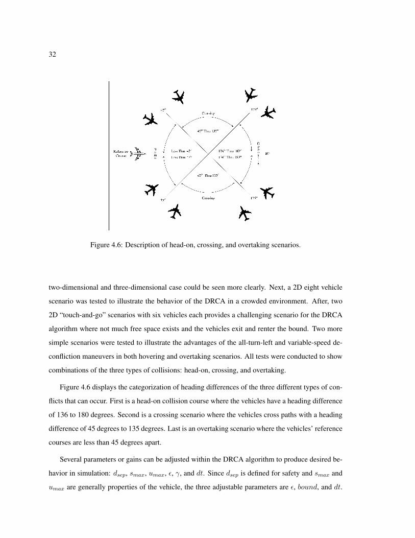
Figure 4.6: Description of head-on, crossing, and overtaking scenarios.
two-dimensional and three-dimensional case could be seen more clearly. Next, a 2D eight vehicle
scenario was tested to illustrate the behavior of the DRCA in a crowded environment. After, two
2D “touch-and-go” scenarios with six vehicles each provides a challenging scenario for the DRCA
algorithm where not much free space exists and the vehicles exit and renter the bound. Two more
simple scenarios were tested to illustrate the advantages of the all-turn-left and variable-speed de-
confliction maneuvers in both hovering and overtaking scenarios. All tests were conducted to show
combinations of the three types of collisions: head-on, crossing, and overtaking.
Figure 4.6 displays the categorization of heading differences of the three different types of con-
flicts that can occur. First is a head-on collision course where the vehicles have a heading difference
of 136 to 180 degrees. Second is a crossing scenario where the vehicles cross paths with a heading
difference of 45 degrees to 135 degrees. Last is an overtaking scenario where the vehicles’ reference
courses are less than 45 degrees apart.
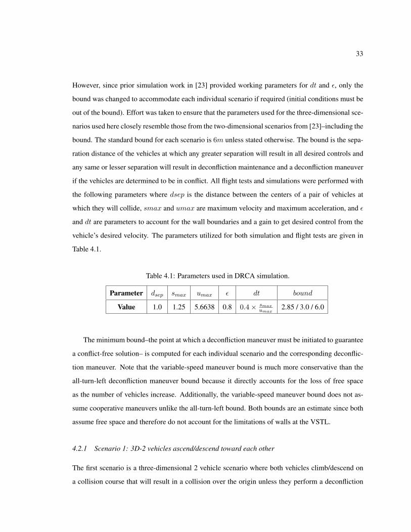
Several parameters or gains can be adjusted within the DRCA algorithm to produce desired be-
havior in simulation: dsep, smax, umax, ε, γ, and dt. Since dsep is defined for safety and smax and
umax are generally properties of the vehicle, the three adjustable parameters are ε, bound, and dt.
33
However, since prior simulation work in [23] provided working parameters for dt and ε, only the
bound was changed to accommodate each individual scenario if required (initial conditions must be
out of the bound). Effort was taken to ensure that the parameters used for the three-dimensional sce-
narios used here closely resemble those from the two-dimensional scenarios from [23]–including the
bound. The standard bound for each scenario is 6m unless stated otherwise. The bound is the sepa-
ration distance of the vehicles at which any greater separation will result in all desired controls and
any same or lesser separation will result in deconfliction maintenance and a deconfliction maneuver
if the vehicles are determined to be in conflict. All flight tests and simulations were performed with
the following parameters where dsep is the distance between the centers of a pair of vehicles at
which they will collide, smax and umax are maximum velocity and maximum acceleration, and ε
and dt are parameters to account for the wall boundaries and a gain to get desired control from the
vehicle’s desired velocity. The parameters utilized for both simulation and flight tests are given in
Table 4.1.
Table 4.1: Parameters used in DRCA simulation.
Parameter dsep smax umax ε dt bound
Value 1.0 1.25 5.6638 0.8 0.4× smaxumax
2.85 / 3.0 / 6.0
The minimum bound–the point at which a deconfliction maneuver must be initiated to guarantee
a conflict-free solution– is computed for each individual scenario and the corresponding deconflic-
tion maneuver. Note that the variable-speed maneuver bound is much more conservative than the
all-turn-left deconfliction maneuver bound because it directly accounts for the loss of free space
as the number of vehicles increase. Additionally, the variable-speed maneuver bound does not as-
sume cooperative maneuvers unlike the all-turn-left bound. Both bounds are an estimate since both
assume free space and therefore do not account for the limitations of walls at the VSTL.
4.2.1 Scenario 1: 3D-2 vehicles ascend/descend toward each other
The first scenario is a three-dimensional 2 vehicle scenario where both vehicles climb/descend on
a collision course that will result in a collision over the origin unless they perform a deconfliction
34
maneuver. Both vehicles travel at a velocity of 1.0m/s toward their waypoints. This scenario was
tested with both the all-turn-left maneuver and the variable-speed maneuver. A bound of 6m was
used for this scenario to correlate with the 2D scenario from [23]. This scenario is an excellent
example of conflict detection in the three-dimensional coordinate frame utilizing 3D cones since
the bound at which the vehicles deconflict is now the euclidian norm of the tangent, normal, and
binormal relative distance. According to equation (3.9) for the all-turn-left maneuver and (3.20) for
the variable-speed maneuver, a conflict-free maneuver should exist as long as the bound is
‖rall−turn−left‖ ≥ 1.71m ‖rvariable−speed‖ ≥ 1.83m. (4.1)
4.2.2 Scenario 2: 3D-2 vehicles fly at each other with vertical separation
The second scenario utilizes two vehicles where both vehicles maintain constant altitude on a course
that will result in vehicle 1 flying over vehicle 2 at the origin. Both vehicles travel at a velocity of
1.0m/s. This case shows that if vehicles are adequately separated in the z direction (i.e. the 3D
collision cone does not encompass the relative velocity vector), the vehicles will be able to achieve
their desired flight paths. In previous work [24, 23] where only two dimensions were considered,
this scenario would have resulted in an unnecessary deconfliction maneuver. This scenario was
tested with the all-turn-left maneuver. The bound remains the same as in Scenario 1.
4.2.3 Scenario 3: 3D-4 vehicles ascend/descend toward each other
The third scenario utilizes 4 vehicles where all vehicles climb/descend on a collision course that will
meet over the origin if no deconfliction maneuver is performed. Specifically, vehicles 3 and 4 climb
to an altitude of 2.5m at takeoff and vehicles 1 and 2 climb to a corresponding altitude of 0.7m.
Vehicles 3 and 4 descend toward the origin with a velocity of 0.3m/s while vehicles 1 and 2 ascend
at 1.0m/s. The desired waypoints set up a collision course that will meet over the origin if no
deconfliction maneuver is performed. This scenario was tested with both the all-turn-left maneuver
and the variable-speed maneuver. The bound used for this scenario is 6m to match the bound used in
[23] on a similar 2D scenario. This scenario is an excellent example of the 3D DRCA deconfliction
maintenance in action since the vehicles deconflict quickly but remain in bound at different altitudes
as they transition the area. Referring to equations (3.9) and (3.20) again, the minimum bound for
35
this scenario is
‖rall−turn−left‖ ≥ 1.46m ‖rvariable−speed‖ ≥ 3.66m. (4.2)
4.2.4 Scenario 4: 3D-4 vehicles maintaining constant altitude while flying toward each other
The fourth scenario utilizes four vehicles where all vehicles maintain constant altitude on a collision
course that will meet over the origin if no deconfliction maneuver is performed. Specifically, vehi-
cles 2 and 4 climb to an altitude of 2.5m at takeoff and vehicles 1 and 3 climb to a corresponding
altitude of 0.7m. All vehicles maintain constant altitude. The desired waypoints set up a collision
course that will meet over the origin if no deconfliction maneuver is performed. The scenario illus-
trates the robustness of the deconfliction maneuver and 3D collision cone along with the previous
scenario by changing the order in which vehicles will detect conflicts with other vehicles. The ve-
locities and bound are the same as for scenario 3. This scenario was tested with both the all-turn-left
maneuver and the variable-speed maneuver.
The variable-speed maneuver was not tested on scenarios with more than 4 vehicles since the
crowded test space necessitates the existence of the third group of possible velocity vectors: collision
cone intersections. The current version of the variable-speed maneuver checks for the availability
of the nearest velocity vectors outside of the collision cone (right and left) and the intersection of
a collision cone and the vehicle’s maximum velocity point (up to four different possible velocity
vectors). In these congested scenarios, these points tend to be in conflict with another vehicle. The
inclusion of collision cone intersections would essentially solve this problem and will be included
in future work. Nonetheless, the successful tests with four vehicles using the current version of the
variable-speed maneuver is a testament to its robustness.
4.2.5 Scenario 5: 2D 8 Vehicle Scenario
In this scenario, every vehicle climbs to an altitude of 0.7m and attempts to cross through the origin
to the opposite side of the circle formed by the vehicles at a velocity of 1.0m/s. The vehicles
deconflict using the all-turn-left maneuver. Due to the close spacing of each vehicle, a bound of
2.85m was used for this scenario so that the initial conditions would not be cause the vehicles to
36
begin in bound. The all-turn-left deconfliction maneuver bound is
‖rall−turn−left‖ ≥ 1.71m. (4.3)
If the variable-speed maneuver had been used for this case, the vehicles would have to be separated
by
‖rvariable−speed‖ ≥ 8.21m (4.4)
when they began their deconfliction maneuver to guarantee a collision avoidance maneuver exists
(assuming the existence of walls does not hinder the necessary deconfliction velocity). The differ-
ence in bound is primarily based on using the cooperative maneuver assumption for the all-turn-left
maneuver and assuming noncooperative maneuvers for the variable-speed maneuver. However,
the performance of the all-turn-left maneuver in this scenario indicates that the more sophisticated
variable-speed maneuver would work well also.
4.2.6 Scenario 6: 2D 6 Vehicle Touch-and-Go Repeated Waypoint Scenario
All Vehicles climb to 0.7m and proceed to perform a “touch-and-go” scenario with 3 waypoints
total where the 1st and 3rd waypoints are the same. Due to the close spacing of each vehicle, a
bound of 3.0m was used for this scenario to ensure the vehicles were not initiated in bound. The
velocities are the same as Scenario 5, and therefore the all-turn-left bound is the same as well. If the
variable-speed-maneuver had been used for this case, the vehicles would have to be separated by
‖rvariable−speed‖ ≥ 5.91m (4.5)
when they began their deconfliction maneuver to guarantee the existence of a conflict free deconflic-
tion path–assuming the necessary velocity vector will not cause the vehicle to encounter a boundary
of the test space.
4.2.7 Scenario 7: 2D 6 Vehicle Touch-and-Go Unique Waypoint Scenario
All vehicles climb to 0.7m and proceed to perform a “touch-and-go” scenario with 3 waypoints total
where no one waypoint repeated for each vehicle. This causes the vehicles to take off, trade places,
and land in an asymmetric way, so that the vehicles encounter one another at different points in the
37
flight. Again, due to the close spacing of each vehicle, a bound of 3.0m was used for this scenario
to ensure none of the vehicles were initiated in bound. The all-turn-left minimum bound is the same
as scenario 5 and 6. The test is the current method employed by the Boeing VSTL in evaluating the
capability of collision avoidance algorithms. The successful completion of this scenario illustrates
the effectiveness of the DRCA.
4.2.8 Scenario 8: 2D Hovering Scenario
The following scenario illustrates the problem associated with the arbitrary velocity direction from
hovering. The scenario begins with vehicle 1 traveling to the origin while vehicle 2 remains sta-
tionary. Once vehicle 1 is hovering over the origin, vehicle 2 proceeds on a path directly opposite
its original coordinates at a velocity of 1.0m/s which results in a waypoint path through the origin.
Referring to equations (3.9) and (3.20) again, the minimum bound for this scenario is
‖rall−turn−left‖ ≥ 1.35m ‖rvariablespeed‖ ≥ 1.83m. (4.6)
4.2.9 Scenario 9: 2D Overtaking Scenario
Vehicle 1 and vehicle 2 travel in a straight trajectory to the other side of the test space. Vehicle 2
is traveling faster than vehicle 1 at a velocity of 1.0m/s and overtakes vehicle 1 who is traveling at
0.4m/s. Referring to equations (3.9) and (3.20) again, the minimum bound for this scenario is
‖rall−turn−left‖ ≥ 1.49m ‖rvariablespeed‖ ≥ 1.83m. (4.7)
38
Chapter 5
ALL-TURN-LEFT 2D AND 3D SIMULATION AND FLIGHT TEST RESULTS
5.1 All-turn-left 3D Simulation and Flight Test Results
The following four flight tests were conducted at the VSTL. Simulation and flight test results are
presented on the same graph. The remaining scenarios were not tested at the VSTL, but the agree-
ment between simulation results and flight tests in Figures 5.1(a)-5.4(f) are a good indication that
the remaining scenarios would show a corresponding agreement in flight tests.
5.1.1 Scenario 1: 3D-2 vehicles ascend/descend toward each other
The results from testing the first scenario are included in Figures 5.1(a)-5.1(f). Figure 5.1(a) and
5.1(b) display the position of the vehicles as they maneuver around one another. Simulation and
flight test results match well. The vehicles succeed in avoiding each other while remaining in close
proximity to their desired paths. Vehicle 2 performs a slightly wider left turn in the flight test re-
sults, but the separation distance and conflict detection are as expected (Figure 5.1(c) and 5.1(d)).
Each vehicle follows their desired controls, ignoring the conflict, until they come in bound (within
γ). Figure 5.1(c) shows that the vehicles are in conflict until they are in bound and then quickly
resolve the conflict (by both turning left). The deconfliction maintenance process is functional as
the vehicles do not come back into conflict after initial deconfliction. Figure 5.1(d) shows how
close the vehicles come to their defined minimum separation distance, dsep, over time. Most im-
portantly, no collision occurs. In Figure 5.1(e), the controls in the x and y direction (Ux and Uy)
are basically mirror images, since the vehicles are headed directly toward each other, and their pre-
scribed deconfliction maneuver is all-turn-left. After the vehicles take off, they accelerate toward
their waypoints. They both turn hard left after coming within a distance of γ. A hard left for vehicle
1 equates to a positive increase in Ux; for vehicle 2 it is a negative increase in Ux. After decon-
flicting, both vehicles accelerate in the direction opposite their deconfliction maneuvers to reorient
themselves toward their waypoints. There are not many overshoots, and the controls occasionally
39
saturate at 5.6638m/s2, which equates to the maximum acceleration at maximum bank. Note from
Figure 5.1(e) that the vehicles perform their deconfliction maneuver while maintaining the desired
z velocity. Figure 5.1(f) displays the speed of the vehicles while they perform their deconfliction
maneuvers where the speed occasionally saturates as the vehicles deconflict.
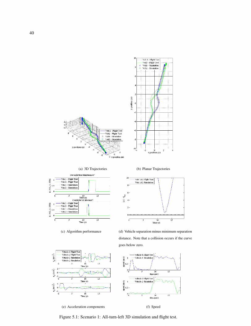
40
(a) 3D Trajectories (b) Planar Trajectories
(c) Algorithm performance (d) Vehicle separation minus minimum separation
distance. Note that a collision occurs if the curve
goes below zero.
(e) Acceleration components (f) Speed
Figure 5.1: Scenario 1: All-turn-left 3D simulation and flight test.
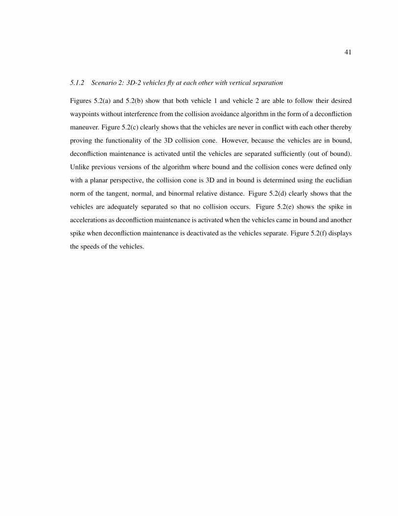
41
5.1.2 Scenario 2: 3D-2 vehicles fly at each other with vertical separation
Figures 5.2(a) and 5.2(b) show that both vehicle 1 and vehicle 2 are able to follow their desired
waypoints without interference from the collision avoidance algorithm in the form of a deconfliction
maneuver. Figure 5.2(c) clearly shows that the vehicles are never in conflict with each other thereby
proving the functionality of the 3D collision cone. However, because the vehicles are in bound,
deconfliction maintenance is activated until the vehicles are separated sufficiently (out of bound).
Unlike previous versions of the algorithm where bound and the collision cones were defined only
with a planar perspective, the collision cone is 3D and in bound is determined using the euclidian
norm of the tangent, normal, and binormal relative distance. Figure 5.2(d) clearly shows that the
vehicles are adequately separated so that no collision occurs. Figure 5.2(e) shows the spike in
accelerations as deconfliction maintenance is activated when the vehicles came in bound and another
spike when deconfliction maintenance is deactivated as the vehicles separate. Figure 5.2(f) displays
the speeds of the vehicles.
42
(a) 3D Trajectories (b) Planar Trajectories
(c) Algorithm performance (d) Vehicle separation minus minimum separation
distance. Note that a collision occurs if the curve
goes below zero.
(e) Acceleration components (f) Speed
Figure 5.2: Scenario 2: All-turn-left 3D simulation and flight test.
43
5.1.3 Scenario 3: 3D-4 vehicles ascend/descend toward each other
Figures 5.3(a) and 5.3(b) show that all vehicles deconflict by performing a left turn. Notice that
vehicles 1 and 4 and vehicles 2 and 3 remain almost exactly the same distance apart for all time,
showing that the system has good symmetry-an expected characteristic of an all-turn-left collision
avoidance algorithm. Vehicles 1 and 2 do not come as close together because they travel around
vehicles 3 and 4. Figure 5.3(c) shows that as soon as the 3D collision cone detects a conflict, a
deconfliction maneuver is performed and deconfliction maintenance takes over until the vehicles
are separated by more than the bound. Figure 5.3(d) shows that all vehicles maintain adequate
separation and no collisions occur. Figure 5.3(e) illustrates that maximum acceleration is achieved
while performing the deconfliction maneuver. Figure 5.3(f) displays the speed of each vehicle.
Again, agreement between simulation and flight tests is observed.
5.1.4 Scenario 4: 3D-4 vehicles maintaining constant altitude while flying toward each other
Figure 5.4(a) and 5.4(b) show that all vehicles deconflict in pairs by performing a left turn. Vehicles
2 and 4 deconflict while vehicles 1 and 3 deconflict. Because of the symmetry of the scenario, all
vehicles achieve the conflicted and in bound status at nearly the same time. As expected, it takes
longer for vehicles 2 and 4 to get out of bound because they are moving at slower velocities. Figure
5.4(c) shows that as soon as the 3D collision cone detects a conflict, a deconfliction maneuver
is performed and deconfliction maintenance takes over until the vehicles are separated by more
than the bound. Figure 5.4(d) clearly shows no collisions and Figure 5.4(e) displays the change in
accelerations as the vehicles deconflict and move back to their waypoints. Figure 5.4(f) displays the
speed of each vehicle. Again, agreement between simulation and flight tests is observed.
5.2 Advantages of the All-Turn-Left Maneuver
The advantages of the all-turn-left maneuver are the simplicity of the maneuver in both computation
time and the expected result. Only O(n) calculations are required to compute the deconfliction
maneuver for all vehicles in simulation. For the actual implementation on hardware where each
vehicle only computes its own deconfliction maneuver, this scales to nearly no computation time.
As such, simulations with large numbers of vehicles are easier to simulate in real time with the

44
(a) 3D Trajectories (b) Planar Trajectories
(c) Algorithm performance (d) Vehicle separation minus minimum separation
distance. Note that a collision occurs if the curve
goes below zero.
(e) Acceleration components (f) Speed
Figure 5.3: Scenario 3: All-turn-left 3D simulation and flight test.

45
(a) 3D Trajectories (b) Planar Trajectories
(c) Algorithm performance (d) Vehicle separation minus minimum separation
distance. Note that a collision occurs if the curve
goes below zero.
(e) Acceleration components (f) Speed
Figure 5.4: Scenario 4: All-turn-left 3D simulation and flight test.
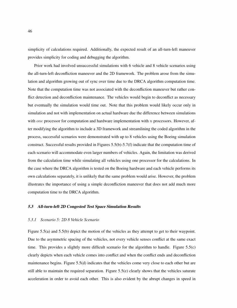
46
simplicity of calculations required. Additionally, the expected result of an all-turn-left maneuver
provides simplicity for coding and debugging the algorithm.
Prior work had involved unsuccessful simulations with 6 vehicle and 8 vehicle scenarios using
the all-turn-left deconfliction maneuver and the 2D framework. The problem arose from the simu-
lation and algorithm growing out of sync over time due to the DRCA algorithm computation time.
Note that the computation time was not associated with the deconfliction maneuver but rather con-
flict detection and deconfliction maintenance. The vehicles would begin to deconflict as necessary
but eventually the simulation would time out. Note that this problem would likely occur only in
simulation and not with implementation on actual hardware due the difference between simulations
with one processor for computation and hardware implementation with n processors. However, af-
ter modifying the algorithm to include a 3D framework and streamlining the coded algorithm in the
process, successful scenarios were demonstrated with up to 8 vehicles using the Boeing simulation
construct. Successful results provided in Figures 5.5(b)-5.7(f) indicate that the computation time of
each scenario will accommodate even larger numbers of vehicles. Again, the limitation was derived
from the calculation time while simulating all vehicles using one processor for the calculations. In
the case where the DRCA algorithm is tested on the Boeing hardware and each vehicle performs its
own calculations separately, it is unlikely that the same problem would arise. However, the problem
illustrates the importance of using a simple deconfliction maneuver that does not add much more
computation time to the DRCA algorithm.
5.3 All-turn-left 2D Congested Test Space Simulation Results
5.3.1 Scenario 5: 2D 8 Vehicle Scenario
Figure 5.5(a) and 5.5(b) depict the motion of the vehicles as they attempt to get to their waypoint.
Due to the asymmetric spacing of the vehicles, not every vehicle senses conflict at the same exact
time. This provides a slightly more difficult scenario for the algorithm to handle. Figure 5.5(c)
clearly depicts when each vehicle comes into conflict and when the conflict ends and deconfliction
maintenance begins. Figure 5.5(d) indicates that the vehicles come very close to each other but are
still able to maintain the required separation. Figure 5.5(e) clearly shows that the vehicles saturate
acceleration in order to avoid each other. This is also evident by the abrupt changes in speed in
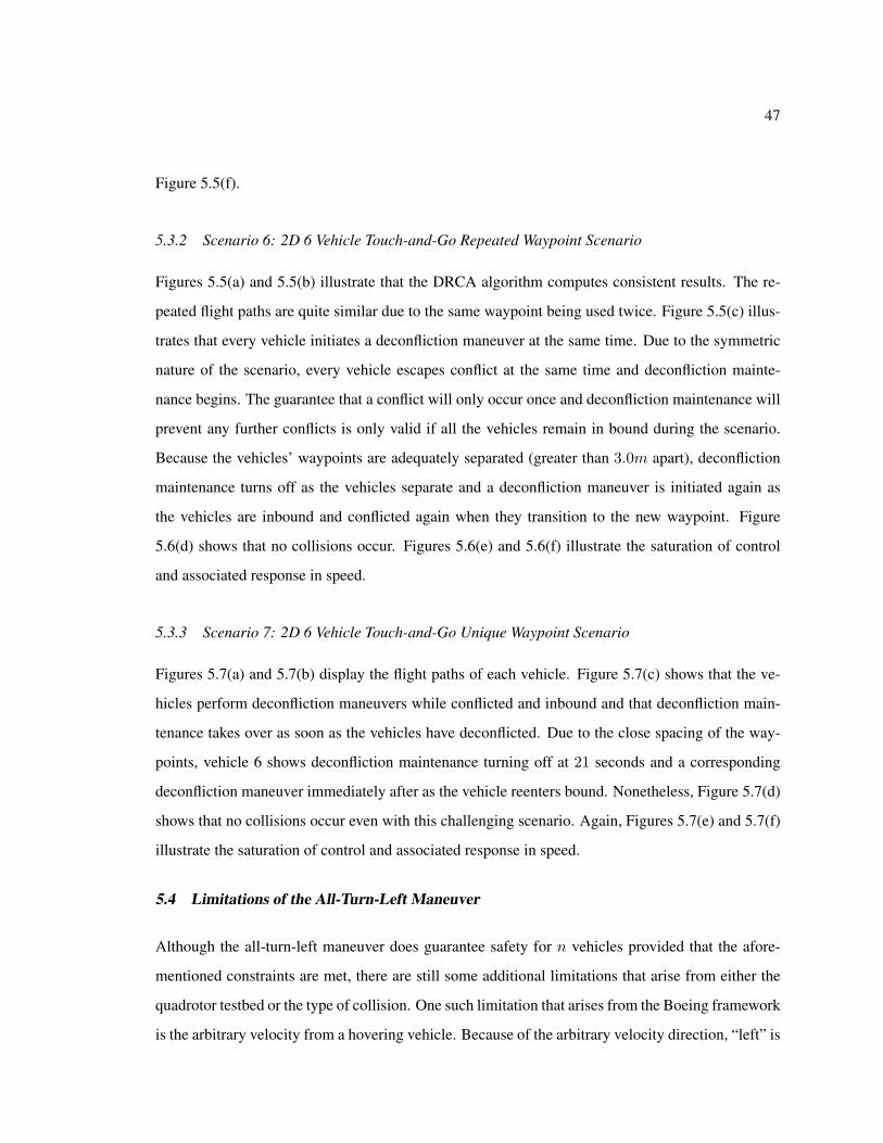
47
Figure 5.5(f).
5.3.2 Scenario 6: 2D 6 Vehicle Touch-and-Go Repeated Waypoint Scenario
Figures 5.5(a) and 5.5(b) illustrate that the DRCA algorithm computes consistent results. The re-
peated flight paths are quite similar due to the same waypoint being used twice. Figure 5.5(c) illus-
trates that every vehicle initiates a deconfliction maneuver at the same time. Due to the symmetric
nature of the scenario, every vehicle escapes conflict at the same time and deconfliction mainte-
nance begins. The guarantee that a conflict will only occur once and deconfliction maintenance will
prevent any further conflicts is only valid if all the vehicles remain in bound during the scenario.
Because the vehicles’ waypoints are adequately separated (greater than 3.0m apart), deconfliction
maintenance turns off as the vehicles separate and a deconfliction maneuver is initiated again as
the vehicles are inbound and conflicted again when they transition to the new waypoint. Figure
5.6(d) shows that no collisions occur. Figures 5.6(e) and 5.6(f) illustrate the saturation of control
and associated response in speed.
5.3.3 Scenario 7: 2D 6 Vehicle Touch-and-Go Unique Waypoint Scenario
Figures 5.7(a) and 5.7(b) display the flight paths of each vehicle. Figure 5.7(c) shows that the ve-
hicles perform deconfliction maneuvers while conflicted and inbound and that deconfliction main-
tenance takes over as soon as the vehicles have deconflicted. Due to the close spacing of the way-
points, vehicle 6 shows deconfliction maintenance turning off at 21 seconds and a corresponding
deconfliction maneuver immediately after as the vehicle reenters bound. Nonetheless, Figure 5.7(d)
shows that no collisions occur even with this challenging scenario. Again, Figures 5.7(e) and 5.7(f)
illustrate the saturation of control and associated response in speed.
5.4 Limitations of the All-Turn-Left Maneuver
Although the all-turn-left maneuver does guarantee safety for n vehicles provided that the afore-
mentioned constraints are met, there are still some additional limitations that arise from either the
quadrotor testbed or the type of collision. One such limitation that arises from the Boeing framework
is the arbitrary velocity from a hovering vehicle. Because of the arbitrary velocity direction, “left” is
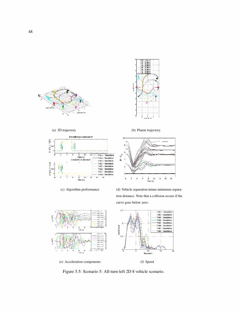
48
(a) 3D trajectory (b) Planar trajectory
(c) Algorithm performance (d) Vehicle separation minus minimum separa-
tion distance. Note that a collision occurs if the
curve goes below zero.
(e) Acceleration components (f) Speed
Figure 5.5: Scenario 5: All-turn-left 2D 8 vehicle scenario.
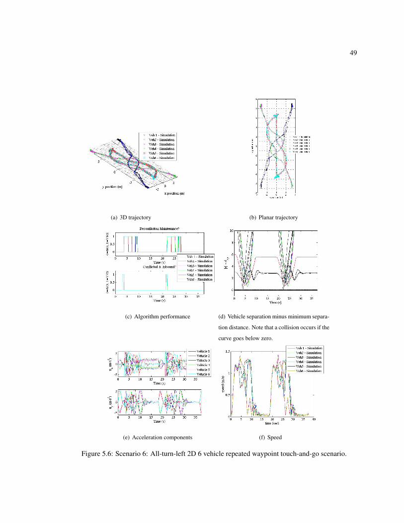
49
(a) 3D trajectory (b) Planar trajectory
(c) Algorithm performance (d) Vehicle separation minus minimum separa-
tion distance. Note that a collision occurs if the
curve goes below zero.
(e) Acceleration components (f) Speed
Figure 5.6: Scenario 6: All-turn-left 2D 6 vehicle repeated waypoint touch-and-go scenario.
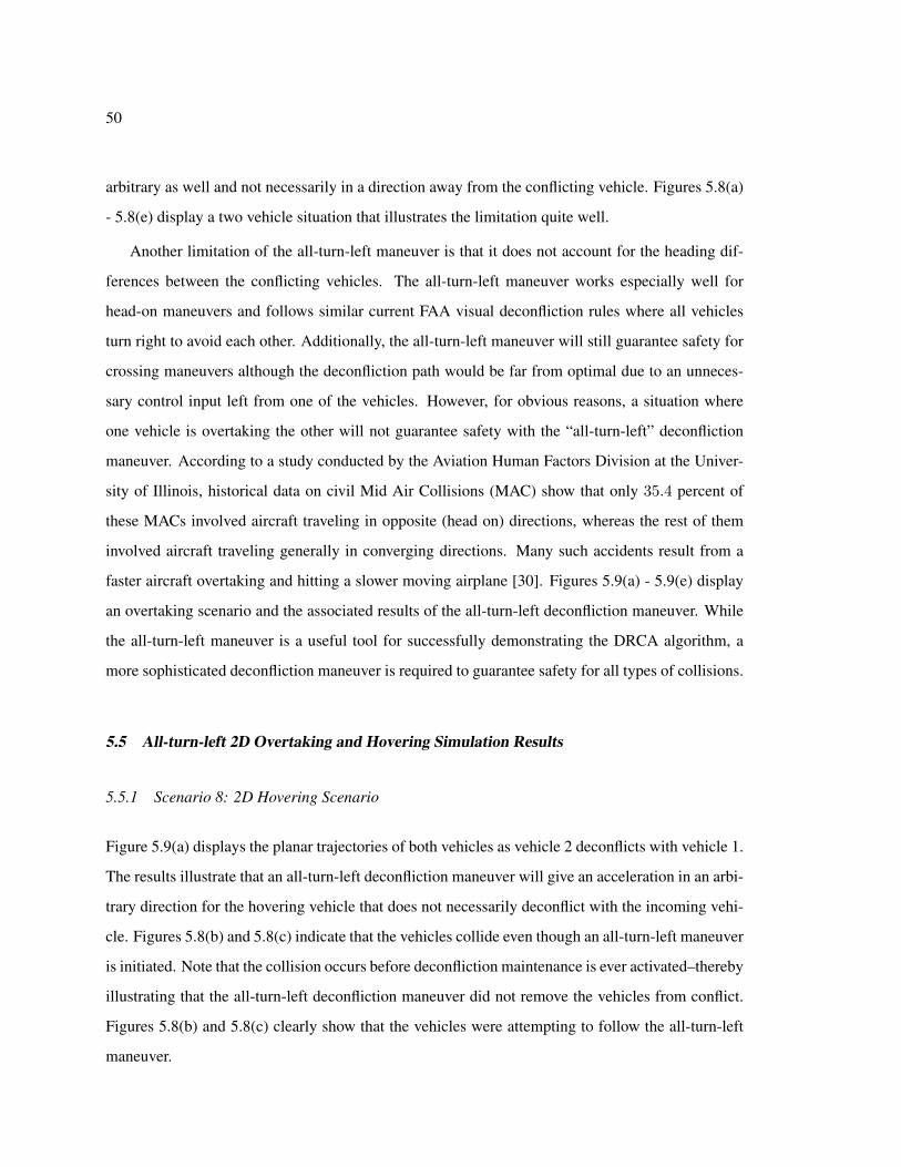
50
arbitrary as well and not necessarily in a direction away from the conflicting vehicle. Figures 5.8(a)
- 5.8(e) display a two vehicle situation that illustrates the limitation quite well.
Another limitation of the all-turn-left maneuver is that it does not account for the heading dif-
ferences between the conflicting vehicles. The all-turn-left maneuver works especially well for
head-on maneuvers and follows similar current FAA visual deconfliction rules where all vehicles
turn right to avoid each other. Additionally, the all-turn-left maneuver will still guarantee safety for
crossing maneuvers although the deconfliction path would be far from optimal due to an unneces-
sary control input left from one of the vehicles. However, for obvious reasons, a situation where
one vehicle is overtaking the other will not guarantee safety with the “all-turn-left” deconfliction
maneuver. According to a study conducted by the Aviation Human Factors Division at the Univer-
sity of Illinois, historical data on civil Mid Air Collisions (MAC) show that only 35.4 percent of
these MACs involved aircraft traveling in opposite (head on) directions, whereas the rest of them
involved aircraft traveling generally in converging directions. Many such accidents result from a
faster aircraft overtaking and hitting a slower moving airplane [30]. Figures 5.9(a) - 5.9(e) display
an overtaking scenario and the associated results of the all-turn-left deconfliction maneuver. While
the all-turn-left maneuver is a useful tool for successfully demonstrating the DRCA algorithm, a
more sophisticated deconfliction maneuver is required to guarantee safety for all types of collisions.
5.5 All-turn-left 2D Overtaking and Hovering Simulation Results
5.5.1 Scenario 8: 2D Hovering Scenario
Figure 5.9(a) displays the planar trajectories of both vehicles as vehicle 2 deconflicts with vehicle 1.
The results illustrate that an all-turn-left deconfliction maneuver will give an acceleration in an arbi-
trary direction for the hovering vehicle that does not necessarily deconflict with the incoming vehi-
cle. Figures 5.8(b) and 5.8(c) indicate that the vehicles collide even though an all-turn-left maneuver
is initiated. Note that the collision occurs before deconfliction maintenance is ever activated–thereby
illustrating that the all-turn-left deconfliction maneuver did not remove the vehicles from conflict.
Figures 5.8(b) and 5.8(c) clearly show that the vehicles were attempting to follow the all-turn-left
maneuver.
51
5.5.2 Scenario 9: 2D Overtaking Scenario
The following scenario illustrates the problem with one vehicle overtaking another. Figure 5.9(a)
displays the planar trajectories of both vehicles as vehicle 2 overtakes vehicle 1. Figure 5.9(b) clearly
shows that both vehicles are in conflict with one another. Figure 5.9(c) show that the vehicles do in
fact collide even though Figures 5.9(d) and 5.9(e) indicate that the vehicles are accelerating to avoid
one another. The scenario demonstrates the insufficiency of an all-turn-left maneuver to guarantee
collision avoidance for all situations.
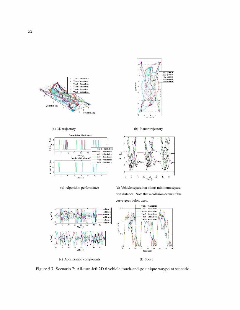
52
(a) 3D trajectory (b) Planar trajectory
(c) Algorithm performance (d) Vehicle separation minus minimum separa-
tion distance. Note that a collision occurs if the
curve goes below zero.
(e) Acceleration components (f) Speed
Figure 5.7: Scenario 7: All-turn-left 2D 6 vehicle touch-and-go unique waypoint scenario.
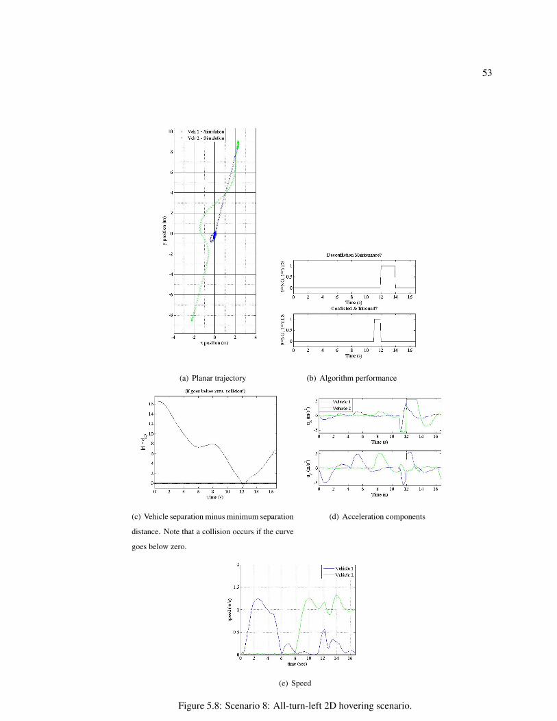
53
(a) Planar trajectory (b) Algorithm performance
(c) Vehicle separation minus minimum separation
distance. Note that a collision occurs if the curve
goes below zero.
(d) Acceleration components
(e) Speed
Figure 5.8: Scenario 8: All-turn-left 2D hovering scenario.
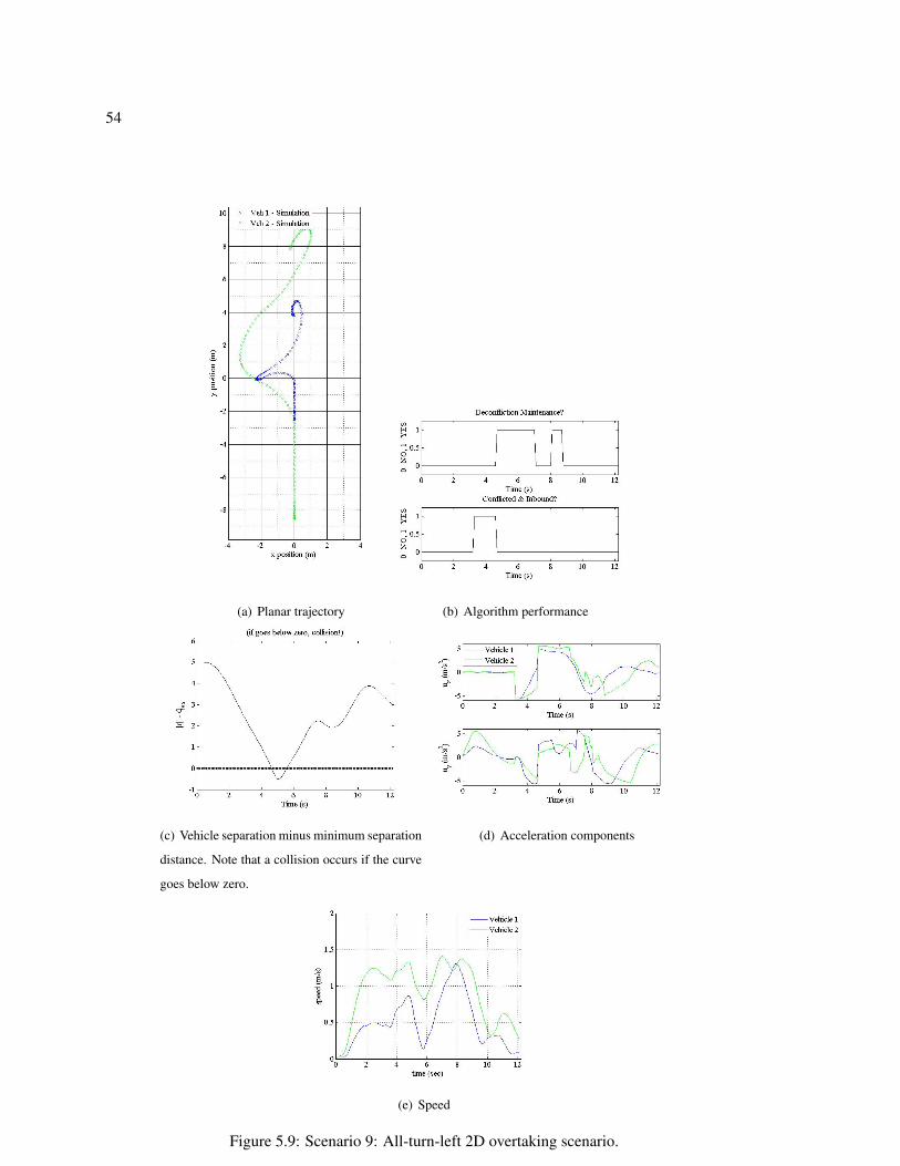
54
(a) Planar trajectory (b) Algorithm performance
(c) Vehicle separation minus minimum separation
distance. Note that a collision occurs if the curve
goes below zero.
(d) Acceleration components
(e) Speed
Figure 5.9: Scenario 9: All-turn-left 2D overtaking scenario.
55
Chapter 6
VARIABLE-SPEED MANEUVER 2D AND 3D SIMULATION
The variable-speed maneuver is an excellent replacement for the all-turn-left deconfliction ma-
neuver because it does not have the same limitations and the computation required still scales well
per vehicle (O(n2)). The results presented here are only from simulation rather than actual flight
tests. However, the results from the previous flight tests illustrate that the simulation is a very good
indication of algorithm performance on actual hardware.
6.1 Advantages of the Variable-Speed Maneuver
The variable-speed maneuver performs quite well in comparison with the all-turn-left deconfliction
maneuver. The variable-speed maneuver directly accounts for the heading difference between the
vehicles in conflict–negating the limitations of the DRCA while using the all-turn-left maneuver.
The following two scenarios show that the limitations of the all-turn-left maneuver are nonexistent
when using the variable-speed maneuver.
6.2 Variable-speed 2D Overtaking and Hovering Simulation Results
6.2.1 Scenario 8: 2D Hovering Scenario
Figure 6.1(a) displays the flight paths of the vehicles as they deconflict. Note that although vehicle
1 has an arbitrary velocity vector while hovering, the algorithm still initiates a control input in the
correct direction to deconflict from vehicle 2. Figure 6.1(b) shows the algorithm performance. The
variable-speed maneuver achieves deconfliction in less than one second and the deconfliction main-
tenance switches on until the vehicles are adequately separated. Figure 6.1(c) shows the expected
result that no collisions occurred. Figure 6.1(d) shows that control saturation was not necessary to
achieve deconfliction. Note that the speed remains below smax while the vehicles deconflict (Figure
6.1(e)).
56
6.2.2 Scenario 9: 2D Overtaking Scenario
Figure 6.2(a) displays the flight paths of the vehicles as they deconflict and achieve their desired
waypoints. Figure 6.2(b) shows that the initial deconfliction maneuver and maintenance phase re-
sulted in the vehicles exiting the bound but then the desired velocity brings the vehicles back in
bound. Again, a deconfliction maneuver is initiated and deconfliction maintenance remains on since
both vehicles remain in bound at their final waypoints. Figure 6.2(c) shows that both vehicles de-
conflict safely with no collisions. Figure 6.2(d) shows some control saturation for vehicle 2 in the
y direction. Otherwise, the vehicles are able to deconflict without much additional control. Figure
6.2(e) displays the difference in speeds where vehicle 2 is traveling faster in order to overtake ve-
hicle 1. The speed increases for both vehicles during the time interval in which they perform their
deconfliction maneuvers. Of primary importance is that the vehicles do not collide as they had with
the all-turn-left deconfliction maneuver shown in Figures 5.9(a)-5.9(e).
6.3 Limitations of the Variable-Speed Maneuver
The obvious limitation of the variable-speed maneuver is computation time. Although computation
time scales well to cn2 per vehicle, simulating all of these vehicles on one processor is much more
computationally intensive than the all-turn-left maneuver. Results indicate that this is a non-issue for
4 or less vehicles. It would be advisable, however, to use more than one processor for simulations
if testing scenarios with more than 4 vehicles–especially if the algorithm is modified to include
collision cone intersections as well.
6.4 Variable-speed 3D Simulation Results
6.4.1 3D-2 vehicles ascend/descend toward each other
The first scenario is a three-dimensional 2 vehicle scenario where both vehicles climb/descend on
a collision course that will result in a collision over the origin unless they perform a deconfliction
maneuver. Figures 6.3(a) and 6.3(b) clearly show that the vehicles deconflict as they proceed to
their waypoints. Figure 6.3(c) illustrates that the vehicles are able to deconflict in less than one
second. Figure 6.3(d) shows that a collision does not occur. Figure 6.3(e) shows that the controls
never saturate during deconfliction or deconfliction maintenance. This is an expected result for the
57
variable-speed-maneuver because the vehicles use only sufficient control to deconflict rather than
the maximum available as in the all-turn-left case. Note that in figure 6.3(f), the vehicles are not
moving in the x and y plane until 8 seconds so that vehicle 1 can climb to the initial position of
z = 2.5m.
6.4.2 3D-4 vehicles ascend/descend toward each other
The third scenario utilizes 4 vehicles where all vehicles climb/descend on a collision course that
will meet over the origin if no deconfliction maneuver is performed. Figures 6.4(a) and 6.4(b)
clearly show that the vehicles deconflict as they proceed to their waypoints. Vehicles 1 and 2 travel
around vehicles 3 and 4. As seen in figure 6.4(c), all vehicles are conflict free within 3 seconds of
conflict detection. Figure 6.4(d) shows that no collisions occurred although vehicles 2 and 4 are at
the minimum separation distance at one point. Figure 6.4(e) shows that the controls never saturate
while deconflicting–indicating that only the sufficient amount of input to avoid a collision is being
used rather than the maximum available. Figure 6.4(f) shows that the vehicles are climbing to their
desired altitude from 0-5.5 seconds and do not begin traveling to their desired destination until this
point. The speed does occasionally show higher values than 1.25m/s although it is evident that the
algorithm does reduce the speed back to the desired maximum relatively quickly. This will not prove
to be an issue in hardware implementation because the maximum speed is a conservative estimate.
Note that the excessive speed occurs during deconfliction maintenance.
6.4.3 3D-4 vehicles maintaining constant altitude while flying toward each other
Figures 6.5(a) and 6.5(b) clearly show that the vehicles deconflict as they proceed to their way-
points. Note that because of the difference in altitudes, vehicle 2 and 4 and 1 and 3 deconflict in
pairs respectively. Note that when vehicle 3 has a substantial deviation in its flight path, it is the
result of the deconfliction maintenance and not the deconfliction maneuver. As seen in figure 6.5(c),
vehicle 3 only takes 1 second to find and broadcast a conflict free velocity so that deconfliction
maintenance begins. Figure 6.5(c) also shows that the variable-speed maneuver was able to find a
conflict free velocity for all vehicles within 3 seconds. Figure 6.5(d) shows that no collisions oc-
curred. Figure 6.5(e) shows that the controls only saturate once while deconflicting–indicating that
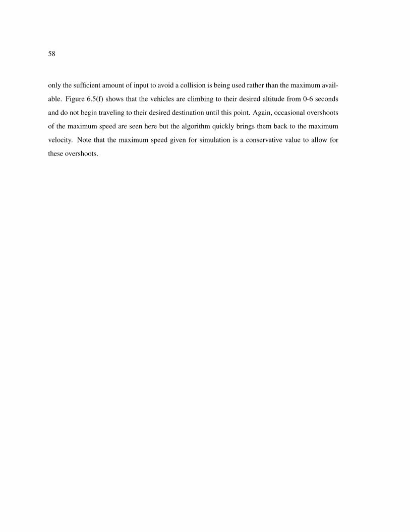
58
only the sufficient amount of input to avoid a collision is being used rather than the maximum avail-
able. Figure 6.5(f) shows that the vehicles are climbing to their desired altitude from 0-6 seconds
and do not begin traveling to their desired destination until this point. Again, occasional overshoots
of the maximum speed are seen here but the algorithm quickly brings them back to the maximum
velocity. Note that the maximum speed given for simulation is a conservative value to allow for
these overshoots.
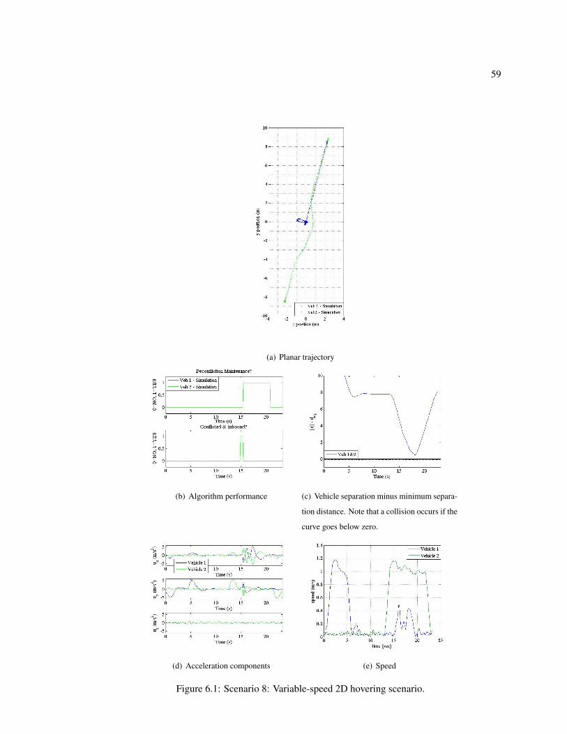
59
(a) Planar trajectory
(b) Algorithm performance (c) Vehicle separation minus minimum separa-
tion distance. Note that a collision occurs if the
curve goes below zero.
(d) Acceleration components (e) Speed
Figure 6.1: Scenario 8: Variable-speed 2D hovering scenario.
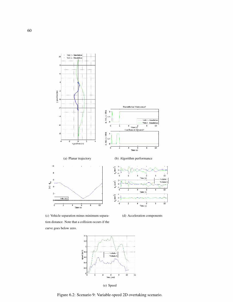
60
(a) Planar trajectory (b) Algorithm performance
(c) Vehicle separation minus minimum separa-
tion distance. Note that a collision occurs if the
curve goes below zero.
(d) Acceleration components
(e) Speed
Figure 6.2: Scenario 9: Variable-speed 2D overtaking scenario.

61
(a) 3D trajectory (b) Planar trajectory
(c) Algorithm performance (d) Vehicle separation minus minimum separa-
tion distance. Note that a collision occurs if the
curve goes below zero.
(e) Acceleration components (f) Speed
Figure 6.3: Scenario 1: Variable-speed 3D simulation.

62
(a) 3D trajectory (b) Planar trajectory
(c) Algorithm performance (d) Vehicle separation minus minimum separa-
tion distance. Note that a collision occurs if the
curve goes below zero.
(e) Acceleration components (f) Speed
Figure 6.4: Scenario 3: Variable-speed 3D simulation.
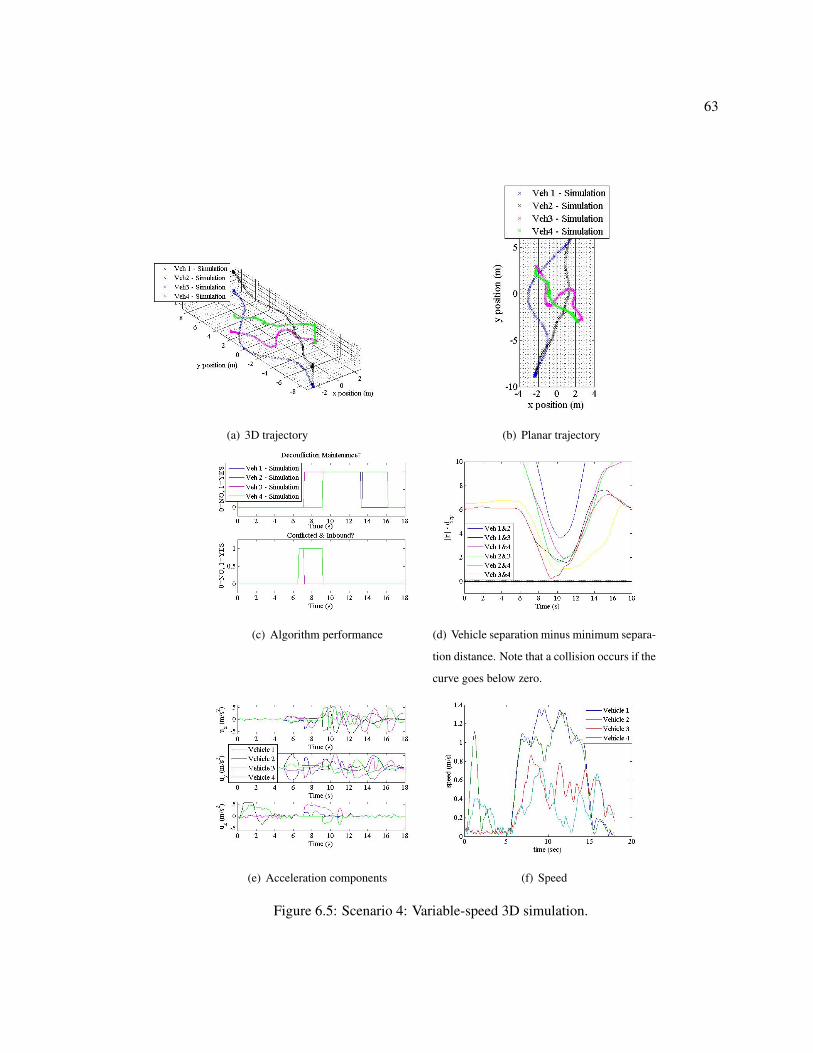
63
(a) 3D trajectory (b) Planar trajectory
(c) Algorithm performance (d) Vehicle separation minus minimum separa-
tion distance. Note that a collision occurs if the
curve goes below zero.
(e) Acceleration components (f) Speed
Figure 6.5: Scenario 4: Variable-speed 3D simulation.
64
Chapter 7
CONCLUSION AND FUTURE WORK
The 3D DRCA algorithm and the variable-speed maneuver deconfliction maneuver were suc-
cessfully implemented on quadrotors at the Boeing VSTL. There are several differences between
the DRCA algorithm implemented in the quadrotors and the algorithm developed in [20]. First, the
variable-speed maneuver does not compute the intersections between collision cones as the slightly
more complex maneuver described in [20]. This modification provides a working algorithm with
O(n2) computations instead of O(n3) as in [20]. Second, the algorithm was modified to allow
one vehicle to hover at any given time during deconfliction if no other solutions exist. Prior work
did not allow the quadrotor to hover during the deconfliction phase. Third, since the system at the
Boeing VSTL is not set up to allow direct modification of acceleration (control), a work-around is
used to convert velocities into controls and vice versa using a new parameter, dt, for the deconflic-
tion maintenance phase while still allowing a velocity input for the deconfliction maneuver phase.
Unfortunately, this method introduces a delay in the system. However, simulations and flight test re-
sults alike indicate that the 3D DRCA algorithm and the variable-speed maneuver are viable systems
for collision avoidance and will be useful for future endeavors at the Boeing VSTL.
Results in this work illustrate the effectiveness of the DRCA algorithm using a 6 vehicle “Touch
and Go” mission script test. As presented in the scenario descriptions, the “Touch and Go” mission
script” causes an even number of vehicles to take off, trade places, and land in an asymmetric way, so
that the vehicles encounter one another at different points in the flight. The test is the current method
employed by the Boeing VSTL in evaluating the capability of collision avoidance algorithms.
Some limitations exist when implementing the 3D DRCA algorithm on quadrotors. First, the
DRCA algorithm was designed for vehicles that could not stop and hover. The DRCA maintenance
phase prevents more than one vehicle hovering within bound at any given time–preventing zero rel-
ative velocity. Second, the enclosed environment and relatively small operating space for multiple
vehicles negates the guarantees for the DRCA algorithm outlined in [20]. Therefore, with the ad-
65
dition of walls, the given bound associated with the all-turn-left and variable-speed deconfliction
maneuvers does not necessarily guarantee a conflict-free path exists.
Further work with the 3D DRCA and corresponding improvements on quadrotors could include
investigating vehicle swarms and formation flight. Although the DRCA algorithm prevents vehicles
from moving in tight formation with identical velocities (vehicles are on the edge of conflict since
m = 0), the relative motion between the vehicles could be stabilized with a separate controller
that guarantees intervehicle spacing. Thus, the DRCA algorithm could be turned off between the
vehicles in formation while still allowing the more difficult tasks such as swarm obstacle avoidance
to be handled by the DRCA. Lalish outlines the theory for this sort of behavior and runs a sim-
ulation of swarming vehicles in [20]. Future work could also include modifying the algorithm to
accommodate the unique quadrotor characteristics and VSTL environment directly. The final piece
of the variable-speed maneuver (collision cone intersections) should be added to the variable-speed
maneuver as in [20] and implemented on the quadrotors. Simulations with both congested test space
and touch-and-go flight paths should be tested to demonstrate robustness. Finally, the DRCA algo-
rithm should be implemented on various other vehicles to observe behavior. The DRCA is optimal
for fixed-wing aircraft with large open areas for deconfliction–as is the case for flight in the NAS.
Simulations and flight tests reproducing such a scenario would be of great benefit to observing the
algorithm’s usefulness.
66
BIBLIOGRAPHY
[1] B. M. Albaker and N. A. Rahim. A survey of collision avoidance approaches for unmannedaerial vehicles. Technical Postgraduates (TECHPOS), 2009 International Conference, Feb2010.
[2] Stefan Bieniawski, Paul Pigg, John Vian, Brett Bethke, and Jon How. Exploring health-enabled mission concepts in the vehicle swarm technology lab. In Proceedings of 2009 In-fotech@Aerospace Conference, Seattle, WA, 2009.
[3] S. Bouabdallah, M. Becker, V. Perrot, and R. Siegwart. Toward obstacle avoidance on quadro-tors. In Proceedings of the XII International Symposium on Dynamic Problems of Mechanics(DINAME 2007), 2007.
[4] C. Carbone, U. Ciniglio, F. Corraro, and S. Luongo. A novel 3d geometric algorithm foraircraft autonomous collision avoidance. In Proceedings of the 45th IEEE Conference onDecision & Control, December 2006.
[5] A. Chakravarthy and D. Ghose. Obstacle avoidance in a dynamic environment: A colli-sion cone approach. IEEE Transactions on Systems, Man, and Cybernetics, 28(5):562–574,September 1998.
[6] L. E. Dubins. On curves of minimal length with a constraint on average curvature and withprescribed initial and terminal positions and tangents. American Journal of Mathematics,79:497–516, 1957.
[7] M. Endsley. Situation awareness, automation & free flight. In FAA/Eurocontrol Air TrafficManagement R&D Seminar, June 1997.
[8] H. Erzberger. Algorithm and operational concept for resolving short range conflicts. Interna-tional Congress of the Aeronautical Sciences, Sept 2008.
[9] D. Esler. How uavs will change aviation. Aviation Week, 2010.
[10] E. Frazzoli, L. Pallottino, V. Scordio, and A. Bicchi. Decentralized cooperative conflict reso-lution for multiple nonholonomic vehicle. In Proc. AIAA Guidance, Navigation and Controlconference, 2005.
[11] R. Ghose and C. J. Tomlin. Maneuver design for multiple aircraft conflict resolution. InProceedings of the American Control Conference, 2000.
67
[12] W. Green and P. Oh. Optic-flow-based collision avoidance applications using a hybrid mav.IEEE Robotics and Automation Magazine, 15(1):96–103, 2008.
[13] David Halaas, Stefan Bieniawski, Paul Pigg, and John Vian. Control and management of anindoor, health enabled, heterogeneous fleet. In Proceedings of the 2009 Infotech@AerospaceConference, Seattle, WA, 2009.
[14] G. Hoffman and C. Tomlin. Decentralized cooperative collision avoidance for accelerationconstrained vehicles. In Proceedings of the 47th IEEE Conference on Decision and Control,December 2008.
[15] T. Horiuchi. A spike-latency model for sonar-based navigation in obstacle fields. IEEE Trans-actions on Circuits and Systems, 56(11):2393–2401, November 2009.
[16] D. B. Kirk, W. S. Heagy, and M. J. Yablonski. Problem resolution support for free flightoperations. IEEE Transactions on Intelligent Transportation Systems, 2:72–80, 2001.
[17] J. Kosecka, C. Tomlin, G. Pappas, and S. Sastry. Generation of conflict resolution maneuversfor air traffic management. In International Conference on Intelligent Robots and Systems(IROS, pages 1598–1603, 1997.
[18] J. Kuchar and L. Yang. A review of conflict detection and resolution modeling methods. IEEETransactions on Intelligent Transportation Systems, 1:179–189, 2000.
[19] P. La Franchi. Near misses between uavs and airliners prompt nato low-level rules review.Flight International, 2006.
[20] E. Lalish. Distributed Reactive Collision Avoidance for Multivehicle Systems. PhD thesis,University of Washington, Seattle, WA, 2009.
[21] E. Lalish and K. Morgansen. Distributed reactive collision avoidance for multivehicle systems.In Proceedings of the IEEE Conference on Decision and Control, 2008.
[22] E. Lalish, K. A. Morgansen, and T. Tsukamaki. Decentralized reactive collision avoidance formultiple unicycle-type vehicles. In Proceedings of the 2008 American Control Conference,Seattle, WA, 2008.
[23] A. Melander. Quadrotor implementation of the distributed reactive collision avoidance algo-rithm. Master’s thesis, University of Washington, Seattle, WA, 2010.
[24] A. Melander, N. Powel, E. Lalish, K. Morgansen, J. Jang, and J. Vian. Implementation ofdeconfliction in multivehicle autonomous systems. Twenty-seventh International Congress ofthe Aeronautical Sciences, Sept 2010.
68
[25] L. Meyn. Nationwide evaluation of a conflict resolution algorithm. 9th AIAA Aviation Tech-nology, Integration, and Operations Conference, Sept 2009.
[26] R. A. Paielli and H. Erzberger. Conflict probability estimation for free flight. Journal ofGuidance, Control, and Dynamics, 20:558–596, 1997.
[27] J. Roberts, T. Stirling, J. Zufferey, and D. Floreano. Quadrotor using minimal sensing forautonomous indoor flight. In 3rd US-European Competetion and Workshop on Micro AirVehicle Systems (MAV07) & European Micro Air Vehicle Conference and Flight Competition(EMAV2007), September 2007.
[28] E. Saad, J. Vian, G. Clark, and S. Bieniawski. Vehicle swarm rapid prototyphing testbed.In AIAA Infotech@Aerospace Conference and AIAA Unmanned...Unlimited Conference, April2009.
[29] D. Shim. An evasive maneuvering algorithm for uavs in sense-and-avoid situations. Master’sthesis, Korea Advanced Institute of Science and Technology, Daejeon, Korea.
[30] N. Taneja and D. Weigmann. Analysis of mid-air collisions in civil aviation. In Proceedings ofthe 45th Annual Meeting of the Human Factors and Ergonomics Society, Santa Monica, CA,2001.
[31] C. Tomlin, G. Pappas, and S. Sastry. Conflict resolution for air traffic management: a study inmulti-agent hybrid systems. IEEE Transactions on Automatic Control, 43:509–521, 1998.
[32] J. Wynbrandt. Collision avoidance strategies and tactics. Technical report, AOPA, Frederick,MD.