Energy Procedia 51 ( 2014 ) 289 – 298

Available online at www.sciencedirect.com

ScienceDirect

1876-6102 © 2013 Elsevier Ltd. This is an open access article under the CC BY-NC-ND license (http://creativecommons.org/licenses/by-nc-nd/3.0/).Selection and peer-review under responsibility of SINTEF Energi ASdoi: 10.1016/j.egypro.2014.07.035

7th Trondheim CCS Conference, TCCS-7, June 5-6 2013, Trondheim, Norway

Qualification of a CO2 storage site using an integrated reservoir study

Barbara Di Pasquoa,*, Pierre de Montleaua, Jean-Marc Danielb, Dan Bossie Codreanub aUpstream Gas division, Enel Trade, Via Arno 42, 00198 Rome, Italy

bIFP Energies nouvelles, 92852 Rueil-Malmaison cedex, France

Abstract

In recent years, global concerns about greenhouse gas emissions have stimulated considerable interest in CO2 storage as a potential “bridging technology”, which could reduce significantly CO2 emissions, while allowing fossil fuels to be used until alternative energy sources are more widely deployed. Flow modeling is a relevant step in the characterization of a CO2 storage site, to provide quantitative predictions of reservoir behavior and assessing the uncertainty [1]. The scope of this work is to analyze the impact of CO2 injection in Pliocene offshore water-bearing sands potentially suitable for CO2 storage, through the implementation of an integrated reservoir study. The approach undertaken was first to build several geological models (local and regional), stochastically populate them with petrophysical properties and, through the gathering and generation of representative dynamic data, develop a dynamic model to simulate a set of possible CO2 injection scenarios. Furthermore a base case scenario was identified to perform a comparison between two different simulators: COORESTM, a code designed by IFPEN, and ECLIPSE300 - CO2STORETM, the Schlumberger compositional tool designed specifically for CO2 storage in saline aquifers. © 2013 The Authors. Published by Elsevier Ltd. Selection and peer-review under responsibility of SINTEF Energi AS.

Keywords: CO2 storage, compositional simulation, characterization

* Corresponding author. Tel.: +39-06-83052951 fax: +39-06-83058485.

E-mail address: barbara.dipasquo@enel.com

© 2013 Elsevier Ltd. This is an open access article under the CC BY-NC-ND license (http://creativecommons.org/licenses/by-nc-nd/3.0/).Selection and peer-review under responsibility of SINTEF Energi AS

290 Barbara Di Pasquo et al. / Energy Procedia 51 ( 2014 ) 289 – 298

1. Introduction

This paper presents the integrated reservoir study performed during the assessment of a potential CO2 storage site. One of the areas identified during a first regional screening study is a deep saline aquifer at a depth of around 2200 m in a formation constituted by Pliocene sands. The approach undertaken was first to build several geological models (local and regional), stochastically populate them with static parameters and, through the gathering and generation of representative dynamic data, develop a reservoir model, simulating a set of possible CO2 injection scenarios. Three main phases, described below, are shown in Fig.1:

Data gathering: the input consists in data coming from eight boreholes and in a 440 km2 of 3D seismic dataset, acquired during a previous hydrocarbon exploration campaign and re-interpreted in order to build the structural model. Core measurements were performed at IFPEN laboratories, the results of which were interpreted to build the petrophysical model and generate relative permeability curves. PVT data, rock compressibility, cap-rock threshold entry pressure and fracturation gradient, were taken from literature.

Modeling: two geological grids, at local and regional scale (the latter being just a volume extension of the former), were generated and populated following a stochastic approach for the generation of the petrophysical model. A sensitivity analysis was performed on the local model accounting for the uncertainty associated with the reservoir heterogeneity.

Simulation: the software used for the simulations was COORESTM, a code designed by IFPEN. Many sensitivities were performed in order to analyze the impact of relevant factors on pressure distribution and CO2 plume spread. A base case for the local model was identified to operate with one well injecting supercritical CO2 for ten years at a rate of 1 Mton/y, followed by a hundred years observation period. Further simulations were run on an extended grid (regional model), increasing the injection rate up to 10 MtonCO2/y, followed by an observation period of one thousand years, that could be extended in future analysis. The software normally used to perform dynamic simulations are either borrowed from the petroleum industry,

with some adjustments, or “recently” customized for the CO2 store injection. Thus, it becomes noteworthy to compare the forecast coming from different tools. A base case scenario for the regional model was used to evaluate the difference in the simulation performance between COORESTM and ECLIPSE300 - CO2STORETM, the Schlumberger compositional tool designed specifically for CO2 storage in saline aquifers.

Finally, a preliminary sensitivity study concerning trapping mechanisms involved in the process was done, including an evaluation of the molecular diffusion impact.

Fig. 1. Work flow overview

Barbara Di Pasquo et al. / Energy Procedia 51 ( 2014 ) 289 – 298 291

2. Data gathering and modeling

2.1. Static reservoir models (Local and Regional)

Two main tasks were performed by IFPEN, aimed at building the static model: structural modeling including the 3D grid building and petrophysical modeling, both achieved using SKUA-GOCADTM software (Paradigm). The set of data used as input for the models was available from a previous hydrocarbon campaign and consists of seismic and borehole data, including some core samples available for laboratory measurements. It was decided to model only the reservoir volume.

Major horizons and faults were used along with stratigraphic column, well correlation, log analysis and a regional permeability (k) vs. porosity (Φ) relationship (Fig. 2) to build a fine scale local geological model, covering an area of about 7x10 km2 with an average cell size of 150x150x10m.The model is limited southwestward by a major thrust, considered sealing, while the other geometrical lateral boundaries can be considered open or closed in the dynamic simulation.

Fig. 2. Examples of data used to build the local geological model– a) well log correlation; b) regional k/Φ relationship;

The geological model was populated through a stochastic method (Sequential Gaussian), exploring the reservoir heterogeneity by means of three correlation lengths (isotropic variogram ranges of 5000 m, 3000 m and 500 m), thus leading to three realizations of the local model. Since no relevant impact on the injection performances were observed in any of the cases, it was decided to use the medium case (variogram range of 3000 m representing the off-set between correlated wells). The regional model covers a larger area (24x26 km2) compared to the local one (Fig.3), while the structural and petrophysical modeling methodology applied are the same.

The fine scale models (both local and regional) were upscaled in a coarser grid, using a cell volume weighted average for porosity and a numerical method based on steady state fluid flow simulations for permeability.

Fig. 3. Regional model – (a) volume of the local and regional models (coarse grid); (b) porosity distribution; (c) permeability distribution

292 Barbara Di Pasquo et al. / Energy Procedia 51 ( 2014 ) 289 – 298

2.2. Dynamic Model and Storage criteria

The cells of the coarse dynamic grid have the following dimensions:

Local model: 250x250m with variable layer thickness ranging from around 30 m to 100 m Regional model: 500x500m with variable layer thickness ranging from around 30 m to 100 m

Dynamic parameters were taken from literature (PVT data, rock compressibility). Drainage relative

permeability curves were estimated from the results of high pressure mercury injection experiments performed in the IFPEN laboratories. The measured capillary pressure curves (Fig.4.a) were collapsed into a dimensionless curve (Leverett J-Curve), representative of the reservoir (Fig.4.b). The relative permeability curves for the wetting and non-wetting phases were calculated according to the Brooks-Corey method through the linearization process of the J-curve, [2] and a rescaling based on end-points taken from literature [3].

Fig. 4. Method used to generate the relative permeability curves: (a) capillary pressure measured at the lab; (b) dimensionless Leveret-J curve in a log-log plot; (c) relative permeability curves

Data used as safety criteria for all simulations are the cap-rock threshold pressure (Pth) and the fracturing pressure (Pfrac)considered as maximum values not to be exceeded during the operations, on which a reasonable safety coefficient (10-20%) has to be applied. Since no measured data were available, both values were estimated from literature.

The fracturation gradient assumed is in line with regional data and is equal to 0.17 bar/m [4], as shown in Fig. 5. In the injection zone, the maximum allowed overpressure ranges from 170 bar to 200 bar, from top to bottom.

Regarding the threshold entry pressure of the cap-rock, the relationship usually used for CH4 storage design was applied [5], correcting it by taking into account the different interfacial tension for CO2. Assuming a cap-rock permeability of 10-6 md, the value considered is 96.62 bar.

Fig. 5. Comparison of the fracturation and pore pressure gradient. The zone highlighted in green corresponds to the injection interval

Barbara Di Pasquo et al. / Energy Procedia 51 ( 2014 ) 289 – 298 293

3. Simulation results

3.1. Simulations performed on the local model

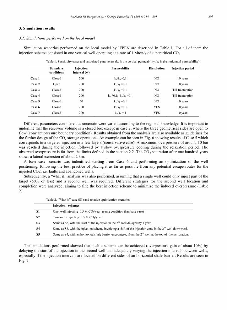
Simulation scenarios performed on the local model by IFPEN are described in Table 1. For all of them the injection scheme consisted in one vertical well operating at a rate of 1 Mton/y of supercritical CO2.

Table 1. Sensitivity cases and associated parameters (kv is the vertical permeability, kh is the horizontal permeability).

Different parameters considered as uncertain were varied according to the regional knowledge. It is important to

underline that the reservoir volume is a closed box except in case 2, where the three geometrical sides are open to flow (constant pressure boundary condition). Results obtained from the analysis are also available as guidelines for the further design of the CO2 storage operations. An example can be seen in Fig. 6 showing results of Case 5 which corresponds to a targeted injection in a few layers (conservative case). A maximum overpressure of around 10 bar was reached during the injection, followed by a slow overpressure cooling during the relaxation period. The observed overpressure is far from the limits defined in the section 2.2. The CO2 saturation after one hundred years shows a lateral extension of about 2 km.

A base case scenario was indentified starting from Case 6 and performing an optimization of the well positioning, following the best practice of placing it as far as possible from any potential escape routes for the injected CO2, i.e. faults and abandoned wells.

Subsequently, a “what if” analysis was also performed, assuming that a single well could only inject part of the target (50% or less) and a second well was required. Different strategies for the second well location and completion were analyzed, aiming to find the best injection scheme to minimize the induced overpressure (Table 2).

Table 2. “What-if” case (S1) and relative optimization scenarios

Injection schemes

S1 One well injecting 0.5 MtCO2/year (same condition than base case)

S2 Two wells injecting 0.5 MtCO2/year

S3 Same as S2, with the start of the injection in the 2nd well delayed by 1 year.

S4 Same as S3, with the injection scheme involving a shift of the injection zone in the 2nd well downward.

S5 Same as S4, with an horizontal shale barrier encountered from the 2nd well at the top of the perforation.

The simulations performed showed that such a scheme can be achieved (overpressure gain of about 10%) by

delaying the start of the injection in the second well and adequately varying the injection intervals between wells, especially if the injection intervals are located on different sides of an horizontal shale barrier. Results are seen in Fig. 7.

Boundary conditions

Injection interval (m)

Permeability Dissolution Injection period

Case 1 Closed 200 kv/kh=0,1 NO 10 years

Case 2 Open 200 kv/kh =0,1 NO 10 years

Case 3 Closed 200 kv/kh =0,1 NO Till fracturation

Case 4 Closed 200 kh *0,1; kv/kh =0,1 NO Till fracturation

Case 5 Closed 50 kv/kh =0,1 NO 10 years

Case 6 Closed 200 kv/kh =0,1 YES 10 years

Case 7 Closed 200 kv/kh = 1 YES 10 years

294 Barbara Di Pasquo et al. / Energy Procedia 51 ( 2014 ) 289 – 298

Fig.6. Case 5 simulation results: overpressure during injection (a) and relaxation (b) periods; (c) model maximum and minimum overpressure vs time; (d) evolution of the CO2 plume after injection (100 years).

Barbara Di Pasquo et al. / Energy Procedia 51 ( 2014 ) 289 – 298 295

Fig.7. Optimization Simulation Results

3.2. Simulations performed on the Regional model

Simulations on the regional model were performed for the base case identified for the local model and an "high rate" injection scenario (10 MtCO2/yr), with an observation time of one thousand years. Here only the results for the "high" case are shown (Fig.8), since, for the base case, as expected, no relevant differences were observed compared to the local model. The base case was used mainly for the software comparison, as seen in the following section. The overpressures reached in the high case still remain inside the safety range, with a maximum value of 55 bar, but, after one thousand years, the CO2 plume reaches the bottom of the cap-rock. Anyway, this cannot be considered as a high risk since the overpressure does not reach the threshold pressure value.

Fig.8. Regional Model Simulation: (a) model maximum and minimum overpressure vs time; (b) CO2 saturation 1000 year after the injection

3.3. Software comparison

The base case scenario for the regional model was used to evaluate the difference in the simulation performance between COORESTM and ECLIPSE300 - CO2STORETM, currently utilized in Enel-Upstream Gas division.

The initialization of the dynamic model was performed considering the same static and dynamic parameters in order to start from the same initial conditions.

A two-phase (water, gas) three-components (H2O, CO2, NaCl) model was considered, with a single equilibrium zone in hydrostatic regime. It is worth-noticing that fluid properties and equation of state parameters are intrinsic to the CO2STORE option [6], as well as solubility coefficients. It has also to be noted that the CO2STORE-option takes into account the mutual solubility of CO2 and brine following the Spycer-Pruess model [7, 8]. The mole

5.5

6

6.5

7

7.5

8

8.5

9

9.5

10

10.5

11

11.5

12

0 500 1000 1500 2000 2500 3000 3500 4000 4500

Time - days

Ove

rp -

bar

s

S1 - maxOVERP

S2 - maxOVERP

S3 - maxOVERP

S4 - maxOVERP

S5 - maxOVERP

S1

S2

S3

S4

S5

296 Barbara Di Pasquo et al. / Energy Procedia 51 ( 2014 ) 289 – 298

fraction of CO2 in each phase, among other parameters, depends on thermodynamic equilibrium constants that can be modified in COORES. Therefore, a tuning was applied to obtain the same solubility model, leading to less than 10% difference of dissolved CO2 molar fraction at saturation between the two software.

The results were compared in terms of pressure variation, CO2 saturation and CO2 dissolved in brine, during and after injection, at the well location (Fig.9) and at field scale (Fig.10). At this stage DIFFUSION and SOLID options were not activated.

A detailed analysis of the cells around the well shows very small discrepancies between the two software: generally pressure values are higher for the simulations obtained with COORES with a maximum absolute difference of 1 bar at the cell 26, that has the lowest permeability (Fig.9.a); the same observation can be done for the CO2 free saturation with a difference of smaller than 4% (Fig.9.b).

At a global scale, no significant differences are observed in the evolution of the CO2 plume (Fig.10).

3.4. Trapping mechanism analysis

An analysis of the trapping mechanisms using ECLIPSE300 was carried out, consisting in an estimation of the percentage of free, residual and dissolved CO2 that can be expected in the reservoir, one thousand years after the end of the injection period. Dissolution trapping is characterized by the amount of CO2 dissolved in the brine. The key factors influencing dissolution kinetics are: flow of the supercritical CO2 in the reservoir, dispersion, molecular diffusion, linked to the concentration gradient, and convection, which is due to the density gradient between CO2 enriched brine and original brine [9]. On the other hand, residual CO2 is trapped in the reservoir by local capillary forces, governing the rock–pore interaction during the imbibition phase. To take into account this last mechanism, the hysteresis option was activated in Eclipse.

Fig. 9. Comparison between COORES (green) and Eclipse (blue) simulation results at the well (the k index of the completed cells ranges between 22 and 30 on the x-axis): absolute value and difference in terms of pressure (a) and free gas saturation (b) at 10 years (left side) and 100 years (right side).

Barbara Di Pasquo et al. / Energy Procedia 51 ( 2014 ) 289 – 298 297

Fig. 10. Comparison between COORES and Eclipse simulation at a global scale: cross section zoomed at well location, showing the CO2 plume spread during injection (1 year) and at the end of the injection (10 years). COORES results left side, ECLIPSE results right side.

Since no imbibition lab measurements were acquired on the available cores, a simple rescaling of the drainage relative permeability curves was performed. The residual gas value used during imbibition was taken from literature [10] and is equal to 0.297, while the Killough hysteresis model was applied to generate the scanning curve [11]. The results obtained can be considered as representative of the range of possible free CO2 present in the reservoir: from a maximum value, when no hysteresis is considered (Fig.11.a) to a minimum value in case of activation of residual trapping (Fig.11.b). In both cases, at the beginning of the injection, 100% of CO2 is dissolved since water is under-saturated. At the completed cells, when water reaches saturation, free gas starts to appear, then a rapid decline of the fraction of dissolved CO2 occurs. The following small peak, that can be observed before the end of injection, might be a grid size effect, due to a discrete representation of a continuous front displacement.. Immediately after the injection, a slow increase of dissolved CO2 occurs, due to the dissolution kinetic factors described above.

When residual CO2 is present, i.e. when the hysteresis is activated, all the previous considerations are still valid but dissolution is generally slowed down, because part of the CO2 in gas phase is immobile (red area in Fig.11.b). It has to be noticed that, after 1000 years, almost no free gas is present and CO2 in place is approximately equally distributed in residual and dissolved phases (Fig.11.b).

A local grid refinement around the well would be appropriate to more accurately model the front advance. This should allow to further investigate the initial high rate of change in free/dissolved CO2 and to reduce a possible overestimation of the real dissolution fraction, characterizing the injection phase (first 10 years).

Fig. 11. Free, residual and dissolved CO2 fraction vs time: (a) no hysteresis; (b) with hysteresis

In the last part of this study, a sensitivity was performed including molecular diffusion effect by considering different diffusion coefficient values. No major impact was observed in the range of values taken from literature [9]. The overall effect of diffusion starts to be consistent after 500 years of simulation, dissolved CO2 increases while residual CO2 decreases. A minimal impact is observed on the free CO2 (Fig.12).

298 Barbara Di Pasquo et al. / Energy Procedia 51 ( 2014 ) 289 – 298

Fig. 12. Evolution of free (green line), residual (red line) and dissolved CO2 (Blue line) in time, with and without diffusion effect included.

4. Conclusions

A summary of an integrated reservoir study was presented for the characterization of a CCS project in its screening phase. Simulation results shown that the CO2 plume is confined all along the observation period at operative conditions, and the overpressure remains below the considered threshold values. Therefore, the site is theoretically suitable for storage. Finally, an optimization of the injection strategy, to mitigate the overpressure during the injection phase, showed some leeway in the project concept.

In terms of reservoir simulation, the benchmark performed between two software, namely COORES from IFPEN and ECLIPSE from Schlumberger, showed a good agreement. Adding further complexity in the simulation model allows to analyze how phenomena like hysteresis (mainly) and diffusion (in a lower manner) can impact the long term trapping mechanisms.

Acknowledgements

This work was realized thanks to the collaboration with Enel “Ingegneria e Ricerca” team. We would also like to thank Schlumberger for their support.

References

[1] Chadwick A, Arts R, Bernstone C, May F, Thibeau S; Zweigel P. Best practice for the storage of CO2 in saline aquifers - observations and guidelines from the SACS and CO2STORE projects. Nottingham, UK, British Geological Survey; 2008 ; pp. 267

[2] Brooks RH, Corey AT. Properties of Porous Media affecting fluid flow. Journal of Irrigation and drainage division, Proc. of ASCE; 1966 [3] Bennion B, Bachu S. Relative Permeability Characteristics for supercritical CO2 displacing water in a variety of potential sequestration

zones in the western Canada sedimentary basin, SPE 95547, ATC Conference 9-12 October. Dallas, TX; 2005 [4] Cobianco S, Pitoni E, Ripa G, Perez D, Patey M, Jeanpert J. Evolution of Viscoelastic surfactant systems for frac&Pack operations in

Adriatic Sea fields, Italy. SPE European Formation Damage Conference; Sheveningen, The Netherlands; 25-27 May 2005 [5] Thomas LK, Katz DL, Tek MR. Threshold Pressure Phenomena in Porous Media, SPE 1816. Society of Petroleum Engineers Journal; June

1968; Vol. 8, No 2; 174 - 184 [6] Schlumberger, Eclipse technical description. 2012.1 [7] Spycher N, Pruess K. CO2-H2O mixtures in the geological sequestration of CO2.II. Partitioning in chloride brines at 12-100 C and up to

600 bar. Geochimica et Cosmochimica Acta; 2005;Vol. 69, No. 13, 3309-3320 [8] Spycher N, Pruess K. A Phase-Partitioning Model for CO2-Brine Mixtures at Elevated Temperatures and Pressures: Application to CO2-

Enhanced Geothermal Systems. Transp. Porous Med. Springer; 2July 2009 [9] Iglauer S. Dissolution Trapping of Carbon Dioxide in Reservoir Formation Brine – A Carbon Storage Mechanism, Mass Transfer -

Advanced Aspects, Dr. Hironori Nakajima (Ed.), ISBN: 978-953-307-636-2, InTech, DOI: 10.5772/20206; 2011. Available from: http://www.intechopen.com/books/mass-transfer-advanced-aspects/dissolution-trapping-of-carbon-dioxide-in-reservoir-formation-brine-a-carbon-storage-mechanism

[10] Bennion B, Bachu S. Supercritical CO2 and H2S – Brine Drainage and Imbibition Relative Permeability-Relationships for Intergranular Sandstone and Carbonate Formations. SPE 99326, SPE Europec/EAGE Annual Conference and Exhibition Wien, Austria; 12-15 June 2006

[11] Killough J E. Reservoir Simulation with History-dependent Saturation Functions. SPE 5106. Society of Petroleum Engineers Journal; 1976; Vol. 16, No. 1, 37-48.

0,E+00

2,E+07

4,E+07

6,E+07

8,E+07

1,E+08

1,E+08

1,E+08

0 100 200 300 400 500 600 700 800 900 1000

GAS I

N PL

ACE

kg-M

Years

Mobile CO2 Mobile CO2 (Diffusion)Residual CO2 Residual CO2 (Diffusion)Dissolved CO2 Dissolved CO2 (Diffusion)