Qualitative Robustness in Bayesian Inference

Houman Owhadi and Clint ScovelCalifornia Institute of Technology

April 21, 2016

Abstract

The practical implementation of Bayesian inference requires numerical approx-imation when closed-form expressions are not available. What types of accuracy(convergence) of the numerical approximations guarantee robustness and what typesdo not? In particular, is the recursive application of Bayes’ rule robust when subse-quent data or posteriors are approximated? When the prior is the push forward of adistribution by the map induced by the solution of a PDE, in which norm should thatsolution be approximated? Motivated by such questions, we investigate the sensitiv-ity of the distribution of posterior distributions (i.e. of posterior distribution-valuedrandom variables, randomized through the data) with respect to perturbations ofthe prior and data generating distributions in the limit when the number of datapoints grows towards infinity.

1 Introduction and motivations

When we apply Bayesian inference with Gaussian priors and linear observations, wedo not actually compute Bayes’ rule but solve the linear system whose solution is theconditional expectation, and robustness is guaranteed by that of our linear solver. Thispaper is motivated by robustness questions that arise in the numerical implementationof Bayes’ rule for continuous systems when closed-form expressions are not available forthe computation of posterior values/distributions. For example, what is the sensitivityof posterior values or the sensitivity of the distribution of posterior values to pertur-bations introduced by the numerical approximation of the prior? When Bayes’ ruleis applied in a recursive manner and approximated posterior distributions are used asprior distributions or approximated data is used in the conditioning process, do we haverobustness guarantees on subsequent posterior distributions/values? Is it possible tonumerically approximate the optimal prior/mixed strategy of a decision theory problem(arising in the continuous setting under the complete class theorem [42]) when closedform expressions are not available, and if it is, in which metric should we do so?

Figure 1.1 provides an illustration of partial answers to such questions, which, whencombined, can be used as a map to navigate robustness/non-robustness questions/issuesarising from numerical approximations. To begin, (a) [34, 33, 35] shows that the range ofposterior values of the quantity of interest under perturbations of the prior in Prokhorov

1

arX

iv:1

411.

3984

v3 [

mat

h.ST

] 2

0 A

pr 2

016

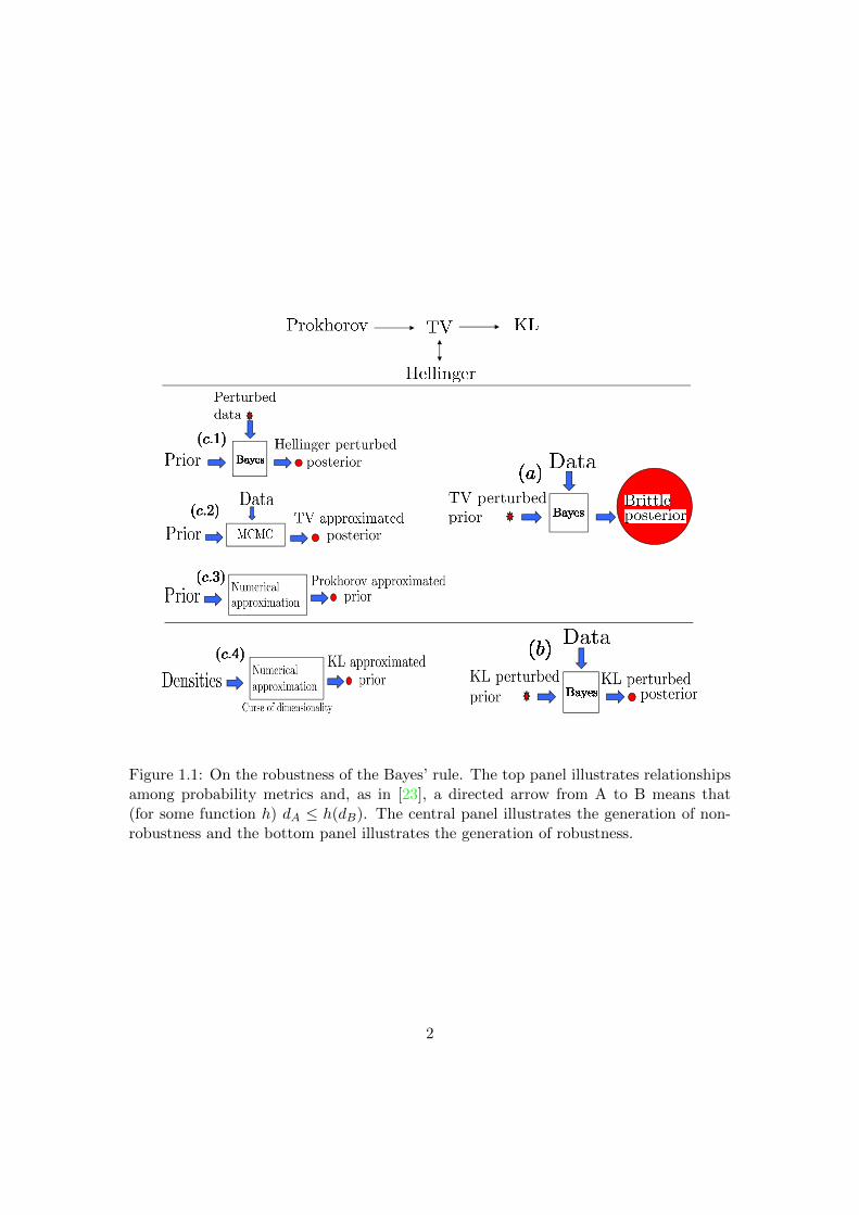
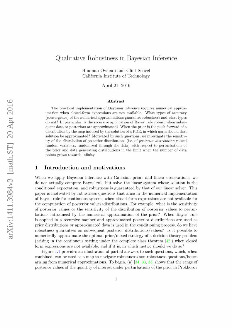
Figure 1.1: On the robustness of the Bayes’ rule. The top panel illustrates relationshipsamong probability metrics and, as in [23], a directed arrow from A to B means that(for some function h) dA ≤ h(dB). The central panel illustrates the generation of non-robustness and the bottom panel illustrates the generation of robustness.

2

or TV metrics is the deterministic range of the quantity of interest (we will refer tothis maximal sensitivity property as brittleness). Moreover, (c.1) [41] shows that theposterior distributions are controlled by the Hellinger metric under the application ofthe Bayes rule with an exact prior under the perturbation of a finite number of finitedimensional samples (see also [11]). Since the Hellinger and TV metrics are equivalent[23], (c.1) and (a) suggest that, without specific restrictions, it is, in general, not pos-sible to offer guarantees on the robustness of recursive Bayes under perturbations ofthe data. Similarly (c.2) the convergence of Markov chains (on continuous state spaces)used in MCMC algorithms (such as the Metropolis algorithm) is generallly analyzedwith respect to the TV topology [38, 22]. However it should be noted that, accordingto Roberts and Rosenthal [37, Pg. 10], Gibbs [22], Gelman [20, Intro] and Madras andSezer [30, Intro], convergence in TV is in general not guaranteed, so that one mightsay in general that convergence of MCMC is at best in TV. Therefore combining (c.2)and (a) suggests that, without further restrictions, it is, in general, not possible to offerguarantees on the robustness of recursive Bayes if posteriors are approximated usingMCMC. Moreover, in many cases, the prior may need to undergo a numerical approx-imation/discretization step prior to conditioning. For example, in popular applicationsof Bayes’ rule to stochastic PDEs [44, 16] one pushes forward the prior from the spaceof coefficients of the PDE to the solution space where it is conditioned. Consequently,if the PDE is numerically approximated this implies an approximation of the pushed-forward prior. Therefore (c.3) representing numerical discretization/approximation asa continuous map between two Polish spaces, it is known that the push forward of ameasure under such maps is continuous in the weak topology, which is metrized by theProkhorov distance. Therefore, combining (c.3) and (a) suggests that, without furtherrestrictions, it is, in general, not possible to offer robustness guarantees to perturbationscaused by the numerical discretization of the prior.

For positive results on the other hand, observe that (b) [24] shows that posteriorvalues (given a finite number of data points) are robust to approximation errors ofthe prior measured in Kullback-Leibler divergence. Therefore if (c.4) the numericalapproximation map is continuous in Kullback-Leibler divergence then posterior values(given a finite number of data points) are robust to that numerical discretization step.However observe that unless closed form expressions are available, one must keep trackof densities to achieve the continuity of the numerical approximation map in Kullback-Leibler divergence, which is a task plagued by the curse of dimensionality.

Since the brittleness of posterior distributions and values with respect perturbationsof the prior defined in TV or Prokhorov metrics is an obstacle to obtaining robustnessguarantees to numerical approximation errors when closed form expressions are unavail-able, it is natural to ask whether robustness could be guaranteed by considering thedistribution of posterior distributions or posterior values generated by the random gen-eration of the data. To answer this question we develop a framework for quantifying thesensitivity of the distribution of posterior distributions with respect to perturbations ofthe prior and data generating distributions in the limit when the number of data pointsgrows towards infinity. In this generalization of Cuevas’ [13] extension of Hampel’s [27]

3

notion of qualitative robustness to Bayesian inference to include both perturbations ofthe prior and the data generating distribution, posterior distributions are analyzed asmeasure-valued random variables (measures randomized through the data) and theirrobustness is quantified using the total variation, Prokhorov, and Ky Fan metrics. Ourresults show that (1) the assumption that the prior has Kullback-Leibler support at theparameter value generating the data, classically used to prove consistency, can also beused to prove the non-robustness of posterior distributions with respect to infinitesimalperturbations (in TV) of the class of priors satisfying that assumption, (2) for a priorwhich has global Kullback-Leibler support on a space which is not totally bounded, wecan establish non-robustness and (3) consistency, and the unstable nature of the condi-tions which generate it, produces non-robustness, and a careful selection of the prior isimportant if both properties (or their approximations) are to be achieved. The mech-anisms supporting our results are different and complementary to those discovered byHampel and developed by Cuevas. To obtain them, we derive in Section 3 a corollaryto Schwartz’ consistency Theorem that leads to robustness or non-robustness resultsdepending on the topology defining the continuity of the numerical approximation map(Kullback-Leibler, TV or Prokhorov). Moreover, this corrollary is further developed inProposition 7.1 to analyze the convergence of random measures in the qualitative robust-ness framework. More precisely, although in [24] it is shown that the Frechet derivativesof posterior values to Kullback-Leibler perturbations of the prior may diverge to infin-ity with the number of data points, a simple application of Proposition 7.1 implies therobustness of the distribution of posterior distributions/values under Kullback-Leiblerperturbations of the prior in the limit where the number of data points goes to infinity.On the other hand, application of Proposition 7.1 also suggest the lack of robustness ofthe distribution of posterior distributions/values to TV or Prokhorov perturbations ofthe prior, where we note that Prokhorov perturbations include classes of perturbationsdefined by generalized moment constraints, as in [8, 6, 7, 5, 34, 33, 35].

2 Qualitative Robustness for Bayesian Inference

Hable and Christmann [25] have recently established qualitative robustness for supportvector machines. Consequently, it appears natural to inquire into the qualitative ro-bustness of Bayesian inference. Hampel [27] introduced the notion of the qualitativerobustness of a sequence of estimators and Cuevas [13] has extended Hampel’s definitionand his basic structural results to Polish spaces. Since the space M(Θ) of priors andposteriors equipped with the weak topology is Polish whenever Θ is, Cuevas’ extensionhas direct applications to Bayesian inference. Boente et al. [10] have developed quali-tative robustness for stochastic processes, Nasser et al. [32] for estimation, and Basu etal.[3] for Bayesian inference with a single sample. The notion of qualitative robustnessintroduce in this paper is a straightforward generalization of that introduced by Hampel[27] and developed by Cuevas [13], see also Cuevas [15]. Indeed, this version requiresno introduction of loss and risk functions and concerns itself with not just expectedvalues but with the full distribution of the effects of the randomness of the observations.

4

It considers a fixed model so is not concerned with robustness with respect to modelspecification, although such considerations can easily be included. Moreover, since itis formulated with respect to classic notions in probability, it appears to us as simple,natural, flexible, without calibration issues, and easy to interpret statistically.

Metrics on spaces of measures and random variables will be important in its formu-lation. Fortunately, this is a well studied field, see e.g. Rachev et al. [36] and Gibbs andSu [23], but to keep the presentation simple, here we will restrict our attention to thetotal variation, Prokhorov and Ky Fan metrics (we refer to [8, 6, 7, 5] for motivationsfor considering classes of priors defined in the Prokhorov metric). For measurable spacesΘ and X, we write M(Θ) and M(X) for the set of probability distributions on Θ andX respectively. In this general setting, we can metrize the spaces of measures M(X)and M(Θ) using total variation. This latter metrization makes M(Θ) into a topologi-cal space whose Borel structure can be used to define the space M2(Θ) of probabilitymeasures on M(Θ), which can also be metrized using the total variation. However, theseparability of these spaces will be extremely useful for us and, in general, these spaceswill not be separable under the total variation metric. Recall that for a metric space(S, d), the Prokhorov metric dPr on the space M(S) of Borel probability measures isdefined by

dPr(µ1, µ2) := infε : µ1(A) ≤ µ2(Aε) + ε, A ∈ B(S)

, µ1, µ2 ∈M(S) , (2.1)

whereAε := x′ ∈ S : d(x, x′) < ε for some x ∈ A .

According to Dudley [18, Thm. 11.3.1], the Prokhorov metric is a metric onM(S). Con-sequently, when Θ and X are metric, , we can also metrize the spaces of measuresM(Θ)and M(X) with the Prokhorov metrics, and having done so we can define the spaceM2(Θ) :=M(M(Θ)) of Borel probability measures on the metric space (M(Θ), dPrΘ)of Borel probability measures on Θ and metrize it with the Prokhorov metric dPr2Θ.Furthermore, when (S, d) is a separable metric space, Dudley [18, Thm. 11.3.3] assertsthat the Prokhorov metric metrizes weak convergence and Aliprantis and Border [1,Thm. 15.12] asserts that the metric space (M(S), dPr) is separable.

Therefore, when X and Θ are separable metric spaces, the Prokhorov metrics dPrXand dPrΘ metrize weak convergence in M(X) and M(Θ) respectively and both metricspaces (M(X), dPrX) and (M(Θ), dPrΘ) are separable. Consequently, when Θ is a sepa-rable metric space, (M(Θ), dPrΘ) is a separable metric space and therefore (M2(Θ), dPr2Θ)is a separable metric space.

The separability of (M(Θ), dPrΘ) is sufficient to define the Ky Fan metric on a spaceof (M(Θ)-valued random variables. Indeed, for a separable metric space S, probabilityspace (Ω,Σ, P ), and two S-valued random variables Z : Ω→ S and W : Ω→ S, the KyFan distance between Z and W , see e.g. Dudley [18, Pg. 289], is defined as

α(Z,W ) := infε ≥ 0 : P (d(Z,W ) > ε) ≤ ε

. (2.2)

By Dudley [18, Thm. 9.2.2], the Ky Fan metric is a metric on the space of S-valuedrandom variables from (Ω,Σ, P ) and metrizes convergence in probability for them. Con-

5

sequently, when Θ is a separable metric space andM(Θ) is metrized with the Prokhorovmetric dPrΘ, the Ky Fan metric α of (2.2) metrizes the space of M(Θ)-valued randomvariables Z : (X∞, µ∞)→ (M(Θ), dPrΘ) for each µ ∈ M(X). Since this family of met-rics depends on the measure µ we indicate this dependence by writing αµ. Moreover,when Θ and X are separable metric spaces, their Borel σ-algebras are countably gener-ated, which is required to apply Doob’s Theorem to assert that a domninated measurablemodel has a jointly measurable family of densities, which is required in the consistencytheorem of Schwartz which we will need.

When Θ and X are Borel subsets of Polish metric spaces, they are separable met-ric spaces so the above applies. Let us now show that the assumption also facilitatesthe measurability of Bayesian conditioning that will be needed to define its qualitativerobustness. To that end, from now on let us place as default the weak topologies onM(X), M(Θ) and M2(Θ) and metrize them with the Prokhorov metrics dPrX , dPrΘand dPr2Θ. This is primarly to obtain well-defined Bayesesian conditioning while atthe same time applicability of Schwartz’s consistency theorem. We will also place othermetric structures on M(X), M(Θ) and M2(Θ) to quantify the size of perturbationsand indicate them with the notation dM(X), dM(Θ) and dM2(Θ). Consider a measurablemodel P : Θ → M(X). Since Aliprantis and Border [1, Thm. 15.13] implies that themap M(X) → R defined by µ 7→ µ(A) is Borel measurable for all A ∈ B(X), it followsthat P corresponds to a Markov kernel. Consider a prior π ∈ M(Θ). Then since Θ isassumed to be a Borel subset of a Polish space, it follows from Schervish [39, Thm. B.46]that there exists a family πx, x ∈ X of conditional probability measures generated by themodel P such that the map x 7→

∫Θ fdπx, x ∈ X is B(X)-measurable for all bounded and

measurable functions f : Θ→ R. Note that after the proof Schervish mentions that sucha family of conditional measures is not unique. Since both Θ and X are separable andmetrizable, it then follows from Aliprantis and Border [1, Thm. 19.7] that the resultingmap x 7→ πx from X to M(Θ) is measurable. For multiple samples, it is clear that Xn

is a Borel subset of the n-th power of the ambient Polish space of X. By Billingsly’s[9, Thm. 2.8] characterization of weak convergence on product spaces it follows that theinjection M(X) → M(Xn) defined by µ 7→ µn is continuous, so that it follows thatPn : Θ → M(Xn), defined by Pn(θ) = P (θ)n, θ ∈ Θ, is measurable and therefore, bythe same arguments as above, we obtain a family of multisample conditional measuresπxn , x

n ∈ Xn such that the resulting map

π : Xn →M(Θ)

defined by the determination of the posteriors

π(xn) := πxn , xn ∈ Xn (2.3)

is measurable. Therefore, its corresponding pushforward operator

π∗ :M(Xn)→M2(Θ)

is well-defined, where we have removed the bar over π in the notation to emphasizethat this pushforward operator π∗ corresponds to the prior π. Then to consider how

6

the posteriors πxn vary as a function of the sample data xn when it is generated byi.i.d. sampling from µ, since Mn(X) ⊂ M(Xn) it follows that µn ∈ M(Xn) so we canutilize the pushforward operator π∗ to define

π∗µn ∈M2(Θ)

the sampling distribution of the posterior distribution πxn when xn ∼ µn.For a fixed prior π ∈ M(Θ), we say that the Bayesian inference is qualitatively

robust at a data generating distribution µ ∈M(X) with respect to an admissible set Pcontaining µ, and metrics dM(X) and dM2(Θ) on M(X) and M2(Θ), if for any ε > 0,there exists a δ > 0 such that

µ ∈ P, dM(X)(µ, µ) < δ =⇒ dM2(Θ)(π∗µn, π∗µ

n) < ε

for large enough n. On the other hand, when the data generating distribution µ is fixedand we vary the prior π, we consider the sequence of maps

πn : X∞ →M(Θ)

defined byπn(x∞) := πxn , x∞ ∈ X∞ . (2.4)

Since the projection Pn : X∞ → Xn is continuous and πn = π Pn, it follows from themeasurability of π : Xn → M(Θ), that πn is measurable, and therefore the resultingsequence

πn : (X∞, µ∞)→M(Θ)

is a sequence of M(Θ)-valued random variables. For each µ ∈ M(X), let αµ be ametric on the space of M(Θ)-valued random variables whose domain is the probabilityspace (X∞, µ∞). Then, for a prior π ∈ M(Θ), we say that the Bayesian inference isqualitatively robust at π with respect to an admissible set Π ⊂M(Θ) containing π andmetrics αµ and dM(Θ) on M(Θ) if given ε > 0, there exists a δ > 0 such that

π ∈ Π, dM(Θ)(π, π) < δ =⇒ αµ(πn, πn) < ε

for large enough n.These two definitions can be combined in a straightforward manner to define robust-

ness corresponding to a single prior/data generating pair. However, to consider a larger

class of distributions than a single pair, we let Z ⊂(M(Θ)×M(X)

)2denote the admis-

sible set of prior-data generating distribution pairs((π, µ), (π, µ)

)∈(M(Θ)×M(X)

)2such that (π, µ) ∈M(Θ)×M(X) is an admissible candidate for robustness and (π, µ) ∈M(Θ) ×M(X) is an admissible candidate for its perturbation. In particular, the pro-jection Z1 ⊂ M(Θ) ×M(X) denotes the set of admissible prior-data generating pairs.Now combining in a straightforward manner we obtain:

7

Definition 2.1. Let X and Θ be Borel subsets of Polish metric spaces and letM(X) andM(Θ) be equipped with the weak topology metrized by the Prokhorov metrics dPrX anddPrΘ. LetM2(Θ) :=M(M(Θ)) be the space of Borel probability measures on the metricspace (M(Θ), dPrΘ) of Borel probability measures on Θ equipped with its weak topologymetrized by its Prokhorov metric dPr2Θ. Consider perturbation pseudometrics dM(X),dM(Θ) and dM2(Θ) onM(X),M(Θ) andM2(Θ) respectively and for each µ ∈M(X), letαµ be a pseudometric on the space ofM(Θ)-valued random variables on the probability

space (X∞, µ∞). Let Z ⊂(M(Θ) ×M(X)

)2denote the admissible set of prior-data

generating distribution pairs and suppose that P : Θ→M(X) is measurable. Then theBayesian inference is qualitatively robust with respect to Z, if given ε1, ε2 > 0, thereexists δ1, δ2 > 0 such that(

(π, µ), (π, µ))∈ Z, dM(Θ)(π, π) < δ1, dM(X)(µ, µ) < δ2

=⇒ dM2(Θ)(π∗µn, π∗µ

n) < ε1 , αµ(πn, πn) < ε2

for large enough n.

Finite sample versions, as introduced in Hable and Christmann [26, Def. 2], are alsoavailable. Note that unlike Hampel and Cuevas who require “for all n” in their defini-tions, we follow Huber [28] and Mizera [31] in only requiring closeness “for large enoughn”. The results of this paper are applicable to both versions. Of course the relevanceof the specific notion of qualitative robustness used depends on the perturbation met-rics used. The results of this paper apply to the case when αµ is the Ky Fan metric,metrizing convergence in probability on the space of M(Θ)-valued random variableswith domain the probability space (X∞, µ∞) and the dM(Θ) is any metric weaker thanthe total variation.

3 Lorraine Schwartz’ Theorem

The fundamental mechanism generating non robustness for Bayesian inference will beits consistency. The breakthrough in consistency for Bayesian inference is consideredto be Schwartz’ theorem [40, Thm. 6.1], so we use it as a model for consistency andthe conditions sufficient to generate it. Stated in Barron, Schervish and Wasserman[2, Intro], Wasserman [43, Pg. 3] and Ghosal, Ghosh and Ramamoorthi [21, Cor. 1]for the nonparametric case, for the parametric case we will operate in Borel subsets ofPolish metric spaces. By Schervish [39, Thm. B.32], regular conditional probabilitiesexist for conditioning random variables with values in such a space. Moreover, when theparametric model is a Markov kernel and is dominated by a σ-finite measure, then bythe Bayes’ Theorem for densities Schervish [39, Thm. 1.31] we have, in addition, that theBayes’ rule for densities determines a valid family of densities for the regular conditionaldistributions. We say that a model P : Θ→M(X) is dominated if there exists a σ-finiteBorel measure ν on X such that Pθ ν, θ ∈ Θ.

8

Recall the Kullback-Leibler divergence K between two measures µ1 and µ2 definedby

K(µ1, µ2) :=

∫log(dµ1

dν

/dµ2

dν

)dµ1 ,

where ν is any measure such that both µ1 and µ2 are absolutely continuous with respectto ν. It is well known that K is nonnegative, and that it is finite only if µ1 µ2, andin that case K(µ1, µ2) =

∫log dµ1

dµ2dµ1 . From this we can define the Kullback-Leibler

ball Kε(µ) of radius ε about µ ∈ M(X) by Kε(µ) = µ′ ∈ M(X) : K(µ, µ′) ≤ ε.For a model P : Θ → M(X), there is the pullback to a function K on Θ defined byK(θ1, θ2) := K(Pθ1 , Pθ2) and when the model is dominated by a σ-finite measure ν, ifwe let p(x|θ) := dPθ

dν (x), x ∈ X be a realization of the Radon-Nikodym derivative, thenthe pullback has the form

K(θ1, θ2) :=

∫log

p(x|θ1)

p(x|θ2)dPθ1(x) .

From this we define a Kullback-Leibler neighborhood of a point θ ∈ Θ by

Kε(θ) :=θ′ ∈ Θ : K(θ, θ′) ≤ ε

.

Let us define the set of priors K(θ) ⊂ M(Θ) which have Kullback-Leibler support at θby

K(θ) :=π ∈M(Θ) : π

(Kε(θ)

)> 0, ε > 0

, (3.1)

which implicitly requires that Kε(θ) be measurable1 for all ε > 0. Also let K ⊂ M(Θ)denote those measures with global Kullback-Leibler support, that is,

K := ∩θ∈ΘK(θ)

is the set of priors which have Kullback-Leibler support at all θ, and let Kae ⊃ K, definedby

Kae :=

π ∈M(Θ) : π

θ ∈ Θ : π

(Kε(θ)

)> 0, ε > 0

= 1

, (3.2)

denote the set of priors with almost global Kullback-Leibler support.Let us address the measurability of the Kullback-Leibler neighborhoods Kε(θ) ⊂

Θ, ε > 0. For the nonparametric case, Barron, Schervish and Wasserman [2, Lem. 11]demonstrate that the Kullback-Leibler neighborhoods Kε(Pθ∗) ⊂M(X) are measurablewith respect to the strong topology restricted to the subspace of measures which areabsolutely continuous with respect to a common σ-finite reference measure. For theparametric case, Dupuis and Ellis [19, Lem. 1.4.3] assert that on a Polish space that Kis lower semicontinuous in both arguments. Since the subset embedding : X → X ′ of

1 Note the change from the standard definition Kε(µ) = µ′ : K(µ, µ′) < ε to ours Kε(µ) = µ′ :K(µ, µ′) ≤ ε does not affect which measures have Kullback-Leibler support, but is more convenientsince then Kε(µ) is closed, simplifying the proof that Kε(θ) is measurable.

9

a subset X of a metric space X ′ is isometric, when X is a Borel subset of a separablemetric space X ′, it can be shown that the induced pushforward map i∗ : M(X) →M(X ′) is isometric in the Prokhorov metrics, in particular it is continuous. Since thecomposition of a continuous and a lower semicontinuous function is lower semicontinuous,it follows from Dupuis and Ellis [19, Lem. 1.4.3] that on any realization of a standardBorel space that the Kullback-Leibler divergence is lower semicontinuous in each of itsarguments separately, in particular, fixing the first, it is lower semicontinuous. ThereforeKε(Pθ∗) ⊂ M(X) is closed, and therefore measurable for ε > 0. Consequently, when Pis measurable, it follows that Kε(θ

∗) ⊂ Θ is measurable for ε > 0.The following corollary to Schwartz’ Theorem, and its implications in Proposition

7.1, gives us the form of consistency that we will use in the robustness analysis. Since theσ-algebra of a Borel subset of a Polish space is countably generated, Doob’s Theorem inDellacherie and Meyer [17, Thm. V.58] and the measurability of the dominated model Pimplies that a family p(θ), θ ∈ Θ of densities can be chosen to be B(X)×B(Θ) measurable,so that this assumption of Schwartz’ Theorem [40, Thm. 6.1] is satisfied. We note thatDellacherie and Meyer emphasize that the countably generated condition is indispensablefor Doob’s Theorem to apply. Note the assumption that the map P : Θ → P (Θ) beopen.

Corollary 3.1 (Schwartz). Let X and Θ be Borel subsets of Polish metric spaces andequip M(X) and M(Θ) with the Prokhorov metrics. Consider an injective measurabledominated model P : Θ→M(X) such that P : Θ→ P (Θ) is open. Then for every π ∈M(Θ) with Kullback-Leibler support at θ∗ ∈ Θ and for every measurable neighborhoodU of θ∗, we have

πxn(U)→ 1 n→∞, a.e. P∞θ∗ .

4 Main Results

Now that we have defined qualitative robustness for Bayesian inference and presentedthe consistency conditions of Schwartz’ Corollary 3.1, we are now prepared for our mainresults. Indeed, the brittleness results of [34, 33, 35] and the non qualitative robustnessresults of Cuevas [13, Thm. 7] suggest that we may obtain non qualitative robustnessaccording to Definition 2.1 by fixing the prior and varying the data generating distribu-tion. However, according to Berk [4], in the misspecified case, although “there need beno convergence (in any sense)”, in the limit the posterior becomes confined to a carrierset consisting of those points which are closest in terms of the Kullback-Leibler diver-gence. Consequently, it appears possible that a generalization of the results of Hampel[27, Lem. 3] and Cuevas [13, Thm. 1] which allows such a set-valued notion of consis-tency may be sufficient. Certainly it will require the more sophisticated notions of thecontinuity, or semi-continuity, of the Kullback-Leibler set-valued information projectionand its dependence on the geometry of the model class P (Θ) ⊂ M(X). Although thispath will certainly be instructive and appears feasible, we instead find it simpler toobtain non qualitative robustness by fixing the data generating distribution to be in

10

the model class and varying the prior. In particular, we show that the inference is notrobust according to Definition 2.1 when the metric αµ is the the Ky Fan metric and themetric M(Θ) is any that is weaker than the total variation metric. It is important tonote that these results do not require any misspecification. Moreover, it appears thatBayesian Inference’s dependence on both the data generating distribution and the priorleads to two complementary mechanisms generating non qualitative robustness; whereasCuevas’ result [13, Thm. 7] utilizes consistency and the discontinuity of the infinite sam-ple limit, this other component utilizes the non-robustness of consistency, namely thatthe set of consistency priors, those with Kullback-Leibler support at the data generatingdistribution, is not robust.

Now let us return to our main results. For θ ∈ Θ, let us recall from (3.1) the set ofpriors K(θ) ⊂ M(Θ) with Kullback-Leibler support at θ and, for ρ > 0, define a totalvariation uniformity Πρ(θ) ⊂M(Θ)×M(Θ) by

Πρ(θ) := (π, π) ∈M(Θ)×M(Θ) : π ∈ K(θ), dtv(π, π) < ρ

of prior pairs where the first component has Kullback-Leibler support at θ and the secondcomponent is within ρ of the first in the total variation metric. For θ ∈ Θ, we define anadmissible set of prior-data generating distribution pairs Zρ(θ) ⊂

(M(Θ)×M(X)

)2by

Zρ(θ) := Πρ(θ)× Pθ × Pθ , (4.1)

using the identification of(M(Θ)×M(X)

)2with M(Θ)2 ×M(X)2.

Our Main Theorem shows, under the conditions of Schwartz’ Corollary, that theBayesian inference is not robust under the assumption that the prior has Kullback-Leibler support at the parameter value generating the data. This result, along with thosethat follow, supports Cuevas’ [14] statement that “his results suggest the possibility ofproving the instability (i.e. the lack of qualitative robustness) for a wide class of usualBayesian models.”

Theorem 4.1. Consider Definition 2.1 with the total variation metric dM(Θ) := dtv onM(Θ) and the Ky Fan metric αµ on the space of M(Θ)-valued random variables withdomain the probability space (X∞, µ∞). Given the conditions of Schwartz’ Corollary3.1, for all θ ∈ Θ the Bayesian inference is not qualitatively robust with respect to Zρ(θ)for all ρ > 0.

Remark 4.2. Actually the proof shows more; let D denote the diameter of Θ, thenfor ε < min (D2 , 1), there does not exist a δ > 0 such that robustness is satisfied. Sincemin (D2 , 1) is large, either half the diameter of the space or larger than 1, we say theinference is brittle.

Theorem 4.1 does not assert that the Bayesian inference is not robust at any specifiedprior, only that it is not robust under the assumption that the prior has Kullback-Leiblersupport at the parameter value generating the data. To establish non-robustness at

11

specific priors we include variation in the data-generating distribution in the model classas follows. Let ∆P ⊂M(X)×M(X), defined by

∆P = (Pθ, Pθ), θ ∈ Θ ,

denote the fact that we allow the data generating distribution to vary throughout themodel class but do not allow any perturbations to it. Then, for π ∈ M(Θ), define the

admissible set Zρ(π) ⊂(M(Θ)×M(X)

)2by

Zρ(π) := π ×Btvρ (π)×∆P ,

where Btvρ (π) is the open ball in the total variation metric.

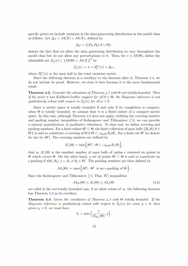
Since the following theorem is a corollary to the theorem after it, Theorem 4.4, wedo not include its proof. However, we state it here because it is the more fundamentalresult.

Theorem 4.3. Consider the sitiuation of Theorem 4.1 with Θ not totally bounded. Thenif the prior π has Kullback-Leibler support for all θ ∈ Θ, the Bayesian inference is notqualitatively robust with respect to Zρ(π) for all ρ > 0.

Since a metric space is totally bounded if and only if its completion is compact,when Θ is totally bounded, we assume that it is a Borel subset of a compact metricspace. In this case, although Theorem 4.3 does not apply, utilizing the covering numberand packing number inequalities of Kolmogorov and Tikhomirov [29], we can providea natural quantification of qualitative robustness. To that end, we define covering andpacking numbers. For a finite subset Θ′ ⊂ Θ, the finite collection of open balls Bε(θ), θ ∈Θ′ is said to constitute a covering of Θ if Θ ⊂ ∪θ∈Θ′Bε(θ). For a finite set Θ′ we denoteits size by |Θ′|. The covering numbers are defined by

Nε(Θ) = min|Θ′| : Θ ⊂ ∪θ∈Θ′Bε(θ)

,

that is, Nε(Θ) is the smallest number of open balls of radius ε centered on points inΘ which covers Θ. On the other hand, a set of points Θ′ ⊂ Θ is said to constitute anε-packing if d(θ1, θ2) ≥ ε, θ1 6= θ2 ∈ Θ′. The packing numbers are then defined by

Mε(Θ) := max|Θ′| : Θ′ is an ε-packing of Θ

.

Since the Kolmogorov and Tikhomirov [29, Thm. IV] inequalities

M2ε(Θ) ≤ Nε(Θ) ≤Mε(Θ) (4.2)

are valid in the not totally bounded case, if we allow values of ∞, the following theoremhas Theorem 4.3 as its corollary.

Theorem 4.4. Given the conditions of Theorem 4.3 with Θ totally bounded. If theBayesian inference is qualitatively robust with respect to Zρ(π) for some ρ > 0, thengiven ε2 > 0, we must have

δ1 < min( 1

N2ε2(Θ), ρ).

12

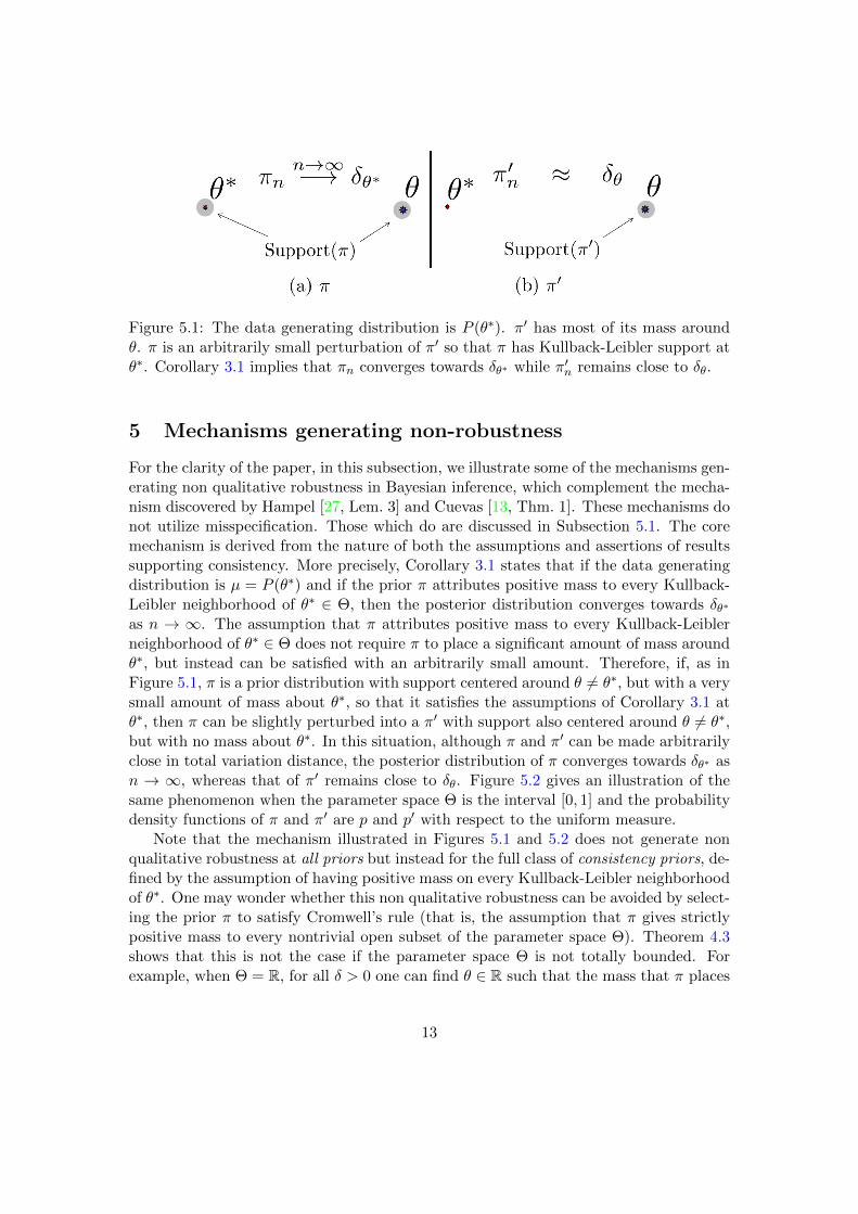
Figure 5.1: The data generating distribution is P (θ∗). π′ has most of its mass aroundθ. π is an arbitrarily small perturbation of π′ so that π has Kullback-Leibler support atθ∗. Corollary 3.1 implies that πn converges towards δθ∗ while π′n remains close to δθ.

5 Mechanisms generating non-robustness

For the clarity of the paper, in this subsection, we illustrate some of the mechanisms gen-erating non qualitative robustness in Bayesian inference, which complement the mecha-nism discovered by Hampel [27, Lem. 3] and Cuevas [13, Thm. 1]. These mechanisms donot utilize misspecification. Those which do are discussed in Subsection 5.1. The coremechanism is derived from the nature of both the assumptions and assertions of resultssupporting consistency. More precisely, Corollary 3.1 states that if the data generatingdistribution is µ = P (θ∗) and if the prior π attributes positive mass to every Kullback-Leibler neighborhood of θ∗ ∈ Θ, then the posterior distribution converges towards δθ∗

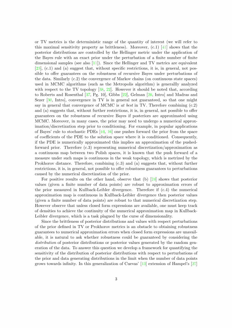
as n → ∞. The assumption that π attributes positive mass to every Kullback-Leiblerneighborhood of θ∗ ∈ Θ does not require π to place a significant amount of mass aroundθ∗, but instead can be satisfied with an arbitrarily small amount. Therefore, if, as inFigure 5.1, π is a prior distribution with support centered around θ 6= θ∗, but with a verysmall amount of mass about θ∗, so that it satisfies the assumptions of Corollary 3.1 atθ∗, then π can be slightly perturbed into a π′ with support also centered around θ 6= θ∗,but with no mass about θ∗. In this situation, although π and π′ can be made arbitrarilyclose in total variation distance, the posterior distribution of π converges towards δθ∗ asn → ∞, whereas that of π′ remains close to δθ. Figure 5.2 gives an illustration of thesame phenomenon when the parameter space Θ is the interval [0, 1] and the probabilitydensity functions of π and π′ are p and p′ with respect to the uniform measure.

Note that the mechanism illustrated in Figures 5.1 and 5.2 does not generate nonqualitative robustness at all priors but instead for the full class of consistency priors, de-fined by the assumption of having positive mass on every Kullback-Leibler neighborhoodof θ∗. One may wonder whether this non qualitative robustness can be avoided by select-ing the prior π to satisfy Cromwell’s rule (that is, the assumption that π gives strictlypositive mass to every nontrivial open subset of the parameter space Θ). Theorem 4.3shows that this is not the case if the parameter space Θ is not totally bounded. Forexample, when Θ = R, for all δ > 0 one can find θ ∈ R such that the mass that π places

13

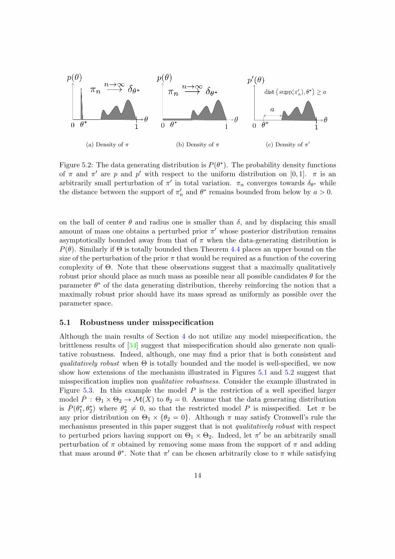
(a) Density of π (b) Density of π (c) Density of π′

Figure 5.2: The data generating distribution is P (θ∗). The probability density functionsof π and π′ are p and p′ with respect to the uniform distribution on [0, 1]. π is anarbitrarily small perturbation of π′ in total variation. πn converges towards δθ∗ whilethe distance between the support of π′n and θ∗ remains bounded from below by a > 0.

on the ball of center θ and radius one is smaller than δ, and by displacing this smallamount of mass one obtains a perturbed prior π′ whose posterior distribution remainsasymptotically bounded away from that of π when the data-generating distribution isP (θ). Similarly if Θ is totally bounded then Theorem 4.4 places an upper bound on thesize of the perturbation of the prior π that would be required as a function of the coveringcomplexity of Θ. Note that these observations suggest that a maximally qualitativelyrobust prior should place as much mass as possible near all possible candidates θ for theparameter θ∗ of the data generating distribution, thereby reinforcing the notion that amaximally robust prior should have its mass spread as uniformly as possible over theparameter space.

5.1 Robustness under misspecification

Although the main results of Section 4 do not utilize any model misspecification, thebrittleness results of [34] suggest that misspecification should also generate non quali-tative robustness. Indeed, although, one may find a prior that is both consistent andqualitatively robust when Θ is totally bounded and the model is well-specified, we nowshow how extensions of the mechanism illustrated in Figures 5.1 and 5.2 suggest thatmisspecification implies non qualitative robustness. Consider the example illustrated inFigure 5.3. In this example the model P is the restriction of a well specified largermodel P : Θ1 ×Θ2 →M(X) to θ2 = 0. Assume that the data generating distributionis P (θ∗1, θ

∗2) where θ∗2 6= 0, so that the restricted model P is misspecified. Let π be

any prior distribution on Θ1 × θ2 = 0. Although π may satisfy Cromwell’s rule themechanisms presented in this paper suggest that is not qualitatively robust with respectto perturbed priors having support on Θ1 × Θ2. Indeed, let π′ be an arbitrarily smallperturbation of π obtained by removing some mass from the support of π and addingthat mass around θ∗. Note that π′ can be chosen arbitrarily close to π while satisfying

14

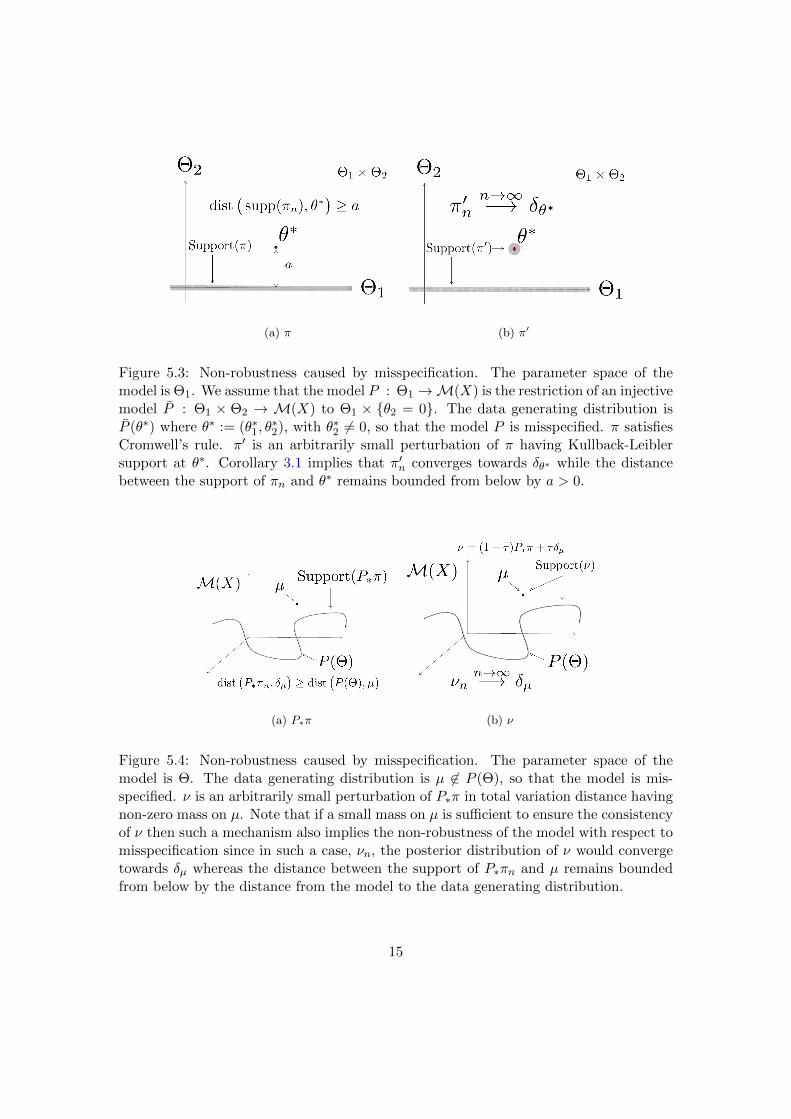
(a) π (b) π′

Figure 5.3: Non-robustness caused by misspecification. The parameter space of themodel is Θ1. We assume that the model P : Θ1 →M(X) is the restriction of an injectivemodel P : Θ1 × Θ2 → M(X) to Θ1 × θ2 = 0. The data generating distribution isP (θ∗) where θ∗ := (θ∗1, θ

∗2), with θ∗2 6= 0, so that the model P is misspecified. π satisfies

Cromwell’s rule. π′ is an arbitrarily small perturbation of π having Kullback-Leiblersupport at θ∗. Corollary 3.1 implies that π′n converges towards δθ∗ while the distancebetween the support of πn and θ∗ remains bounded from below by a > 0.

(a) P∗π (b) ν

Figure 5.4: Non-robustness caused by misspecification. The parameter space of themodel is Θ. The data generating distribution is µ 6∈ P (Θ), so that the model is mis-specified. ν is an arbitrarily small perturbation of P∗π in total variation distance havingnon-zero mass on µ. Note that if a small mass on µ is sufficient to ensure the consistencyof ν then such a mechanism also implies the non-robustness of the model with respect tomisspecification since in such a case, νn, the posterior distribution of ν would convergetowards δµ whereas the distance between the support of P∗πn and µ remains boundedfrom below by the distance from the model to the data generating distribution.

15

the local consistency assumption of Corollary 3.1, which implies that the posterior distri-butions of π′ concentrate on θ∗ while the posterior distributions of π remain supportedon Θ1×θ2 = 0. Note that if P is interpreted as an extension of the model P , then thismechanism suggests that we can establish conditions under which Bayesian inference isnot qualitatively robust under model extension.

Figure 5.4 represents a non-parametric generalization of the mechanism of Figure5.3. Assume that the data generating distribution is µ 6∈ P (Θ), so that the model ismisspecified. Let π ∈ M(Θ) be an arbitrary prior distribution and P∗π ∈ M2(X) itscorresponding non-parametric prior. By removing an arbitrarily small amount of massfrom P∗π and placing it on µ one obtains an arbitrarily close prior distribution ν thatis consistent with respect to the data generating distribution µ. Therefore althoughP∗π and ν may be made arbitrarily close, their posterior distributions would remainasymptotically separated by a distance corresponding to the degree of misspecificationof the model (the distance from µ to P (Θ)).

6 Proofs

6.1 Proof of Corollary 3.1

We seek to apply Schwartz’ theorem [40, Thm. 6.1]. Since Θ and X are separable metricspaces, their Borel σ-algebras are countably generated, so Doob’s Theorem [17, Thm.V.58] and the measurability of the dominated model P implies that a family of densitiescan be chosen to be B(X) × B(Θ) measurable, thus satisfying this requirement of [40,Thm. 6.1]. Since U is a neighborhood it follows that it contains an open neighborhoodO of θ. Since O is open and P : Θ → P (Θ) is open, it follows that P (O) is open inP (Θ), and therefore there is an open set V∗ ⊂ M(X) such that V∗ ∩ P (Θ) = P (O).Moreover, V∗ is an open neighborhood of Pθ∗ . Since X is a separable metric space, itfollows that dPrX metrizes the weak topology, and since V∗ is open, it is well known(see e.g. [2, 43, 21]) that there exists a uniformly consistent test of Pθ∗ against V c

∗ , seeSchwartz [40] for the definition of uniformly consistent test. It follows trivially thatthere exists a uniformly consistent test of Pθ∗ against V c

∗ ∩ P (Θ). Moreover, since P isinjective it follows that Oc = P−1(V c

∗ ). Therefore, there exists a uniformly consistenttest of Pθ∗ against V c

∗ ∩ P (Θ) = Pθ : θ ∈ Oc.Since V∗ is open, it also follows that there is a Prokhorov metric ball Bs(Pθ∗) of

radius s > 0 about Pθ∗ such that Bs(Pθ∗) ⊂ V∗. Now consider the Kullback-Leibler

ball Kτ (Pθ∗) for τ < s2

2 . It follows from Csiszar, Kemperman and Kullback’s [12]improvement K ≥ 1

2d2tv of Pinsker’s inequality and the inequality dtv ≥ dPrX , that

Kτ (Pθ∗) ⊂ Bs(Pθ∗). Since then Kτ (Pθ∗) ⊂ Bs(Pθ∗) ⊂ V∗ it follows that

P−1(Kτ (Pθ∗)

)⊂ P−1(V∗) = O .

Consider now the Kullback-Leibler neighborhood Wτ (θ∗) ⊂ Θ of θ∗ defined by pullingKτ (Pθ∗) back to Θ by the model P :

Wτ (θ∗) := P−1(Kτ (Pθ∗)

).

16

Then the previous inequality states that

Wτ (θ∗) ⊂ O .

Since the Kullback-Leibler neighborhoods are measurable in the weak topology and Pis assumed measurable, it follows that Wτ (θ∗) is measurable.

Therefore, O and Wτ (θ∗) satisfy the assumptions of the sets V and and W in [40,Thm. 6.1]. Consequently, since by assumption, the prior π has Kullback-Leibler support,it follows that we can apply Schwartz’ theorem [40, Thm. 6.1] to obtain the assertionfor O and since U ⊃ O is measurable the assertion follows.

6.2 Proof of Theorem 4.1

Let us prove the assertion for a weaker pseudometric αµ ≤ αµ derived from the Prokhorovmetric on dPr2Θ onM2(Θ). Since it is weaker the assertion follows. To that end, considerµ ∈ M(X). Then for two random variables Z,W : (X∞, µ∞) → M(Θ) it follows thatZ∗µ

∞,W∗µ∞ ∈M2(Θ), so we can define a pseudometric αµ by

αµ(Z,W ) := dPr2Θ(Z∗µ∞,W∗µ

∞) . (6.1)

Since Dudley [18, Thm. 11.3.5] asserts that

dPr2Θ(Z∗µ∞,W∗µ

∞) ≤ αµ(Z,W ) , (6.2)

we conclude thatαµ ≤ αµ . (6.3)

For fixed π and µ and n, the M(Θ)-valued random variable

πn : (X∞, µ∞)→M(Θ)

defined by πn(x∞) := πxn in (2.4) satisfies

(πn)∗µ∞ = π∗µ

n (6.4)

where π∗ : M(Xn) → M2(Θ) is the pushforward operator corresponding to the mapπ : Xn →M(Θ) defined by π(xn) := πxn in (2.3). Consequently, we obtain

αµ(πn, πn) = dPr2Θ(π∗µn, π∗µ

n) (6.5)

for π, π ∈M(Θ) and n fixed. From the triangle inequality we then obtain

dPr2Θ(π∗µn, π∗µ

n) ≤ dPr2Θ(π∗µn, π∗µ

n) + dPr2Θ(π∗µn, π∗µ

n)

≤ αµ(πn, πn) + dPr2Θ(π∗µn, π∗µ

n) ,

bounding the simple single term dPr2Θ(π∗µn, π∗µ

n) in terms of the sum of two termsαµ(πn, πn) and dPr2Θ(π∗µ

n, π∗µn) of qualitative robustness in Definition 2.1. Con-

seuquently, the assumption of the pseudometric αµ amounts to Definition 2.1 with oneepsilon instead of two corresponding to the metric

dPr2Θ(π∗µn, π∗µ

n), (π, π, µ, µ) ∈M(Θ)2 ×M(X)2 . (6.6)

17

Moreover, non qualitative robustness with respect to this definition implies non qualita-tive robustness with respect to the original Definition 2.1 with the Ky Fan metric.

Now lets turn to the proof that the inference is non qualitatively robust with respectto the objective metric (6.6). Fix θ∗ ∈ Θ and consider another point θ ∈ Θ and theDirac mass δθ ∈M(Θ) situated at θ. For π ∈ K(θ∗), the convex combination

πα := απ + (1− α)δθ

is a probability measure with Kullback-Leibler support, that is, πα ∈ K(θ∗), α > 0 and

dtv(πα, δθ) ≤ α. (6.7)

Therefore, it follows that(πα, δθ) ∈ Πρ(θ

∗) , α < ρ ,

and therefore (πα, δθ, Pθ∗ , Pθ∗

)∈ Zρ(θ∗) , α < ρ ,

where Zρ(θ∗) is the admissible set defined in (4.1).For the prior πα, let παn : (X∞, P∞θ∗ )→M(Θ), defined by παn(x∞) := παxn , x

∞ ∈ X∞,denote the corresponding sequence of posterior random variables, and let (παn)∗P

∞θ∗ ∈

M2(Θ) denote its induced sequence of laws. On the other hand, for the prior δθ, it iseasy to see that (δθ)xn = δθ, x

n ∈ Xn, so that if we denote the corresponding sequenceof posterior random variables by δnθ , then (δnθ )∗P

∞θ∗ = (δθ)∗P

nθ∗ = δδθ .

Since the assumptions of Schwartz’ Corollary 3.1 are satisfied and πα has Kullback-Leibler support at θ∗, we can apply the assertion (7.1) of Proposition 7.1

P∞θ∗dPrΘ(παn , δθ∗) > ε

→ 0 n→∞ ,

for ε > 0. To complete the proof we simply use the fact that convergence in law to aDirac mass is equivalent to convergence in probability to a constant random variable,that is use the equivalent assertion (7.2) of Proposition 7.1

dPr2Θ

((παn)∗P

∞θ∗ , δδθ∗

)→ 0 n→∞ . (6.8)

Now the proof is very simple. Indeed, from the triangle inequality we have

dPr2Θ

((παn)∗P

∞θ∗ , δδθ

)≥ dPr2Θ

(δδθ∗ , δδθ

)− dPr2Θ

((παn)∗P

∞θ∗ , δδθ∗

)and, by two applications of Proposition 7.4, we have

dPr2Θ

(δδθ∗ , δδθ

)= min

(dPrΘ

(δθ∗ , δθ

), 1)

= min(

min(d(θ∗, θ), 1

), 1)

= min(d(θ∗, θ), 1

).

18

Therefore, since (δnθ )∗P∞θ∗ = δδθ , the convergence (6.8) implies that

dPr2Θ

((παn)∗P

∞θ∗ , (δ

nθ )∗P

∞θ∗

)→ min

(d(θ∗, θ), 1

), n→∞ .

Finally, since dPrΘ ≤ dtv, it follows from (6.7) that

dPrΘ(πα, δθ) ≤ α.

Then, for any δ > 0, if we restrict α so that α < min (δ, ρ), it follows that dtv(πα, δθ) < ρ

and dPrΘ(πα, δθ) < δ, so that (πα, δθ, Pθ∗ , Pθ∗

)∈ Zρ(θ∗) , (6.9)

dPrΘ(πα, δθ) < δ . (6.10)

Let D := sup d(θ1, θ2) : θ1, θ2 ∈ Θ denote the diameter of Θ. Then it follows from thetriangle inequality that, for any ε > 0, there exists a θ ∈ Θ such that d(θ∗, θ) ≥ D

2 − ε.Consequently, for any ε < min (D2 , 1), no matter how small δ is, there is an α > 0 suchthat, in addition to (6.9) and (6.10), we have

dPr2Θ

((παn)∗P

∞θ∗ , (δ

nθ )∗P

∞θ∗

)> ε ,

for large enough n. Consequently, the assertion is proved.

6.3 Proof of Theorem 4.4

As in the proof of Theorem 4.1, we establish the assertion with respect to the modifiedform of qualitative robustness defined by (6.6), and since this form is weaker it impliesthe assertion. It follows from the definition of the packing numbers that, for ε > 0, thereis a packing θi, i = 1, ..,M2ε(Θ) and therefore the collection of open balls Bε(θi), i =1, ..,M2ε(Θ) is a disjoint union. Denoting N2ε := N2ε(Θ) and M2ε := M2ε(Θ), wetherefore obtain

1 = π(Θ)

≥ π(∪M2εi=1 Bε(θi)

)=

M2ε∑i=1

π(Bε(θi)

)≥ M2ε min

i=1,M2ε

π(Bε(θi)

).

Consequently, since (4.2) implies M2ε ≥ N2ε, there exists a point θ∗ ∈ Θ such that

π(Bε(θ

∗))≤ 1

N2ε. (6.11)

19

Let Bε := Bε(θ∗) denote the open ball about θ∗ and let Bc

ε denote its complement. Letπε ∈M(Θ), defined by

πε(B) :=π(Bc

ε ∩B)

π(Bcε )

, B ∈ B(Θ) ,

denote the normalization of the restriction of π to Bcε which, by the inequality (6.11), is

well defined. Since π = π(Bcε )π

ε + π|Bε it follows that π − πε = π|Bε − π(Bε)πε so that

we obtain

dtv(πε, π) ≤ π(Bε) ≤

1

N2ε

from which we obtain

dPrΘ(πε, π) ≤ 1

N2ε. (6.12)

In particular, when 1N2ε

< ρ, we obtain

πε ∈ Btvρ (π)

and therefore (π, πε, Pθ∗ , Pθ∗

)∈ Zρ(π) .

That is, when 1N2ε

< ρ, the point(π, πε, Pθ∗ , Pθ∗

)∈ Zρ(π).

For the prior πε, let πεn : (X∞, P∞θ∗ )→M(Θ), defined by πεn(x∞) := πεxn , x∞ ∈ X∞,

denote the corresponding sequence of posterior random variables, and let (πεn)∗P∞θ∗ ∈

M2(Θ) denote its induced sequence of laws. Since the assumptions of Schwartz’ Corol-lary 3.1 are satisfied and π has Kullback-Leibler support at θ∗, we can apply the assertion(7.2) of Proposition 7.1 to the sequence of posterior laws (πn)∗P

∞θ∗ corresponding to π:

dPr2Θ

((πn)∗P

∞θ∗ , δδθ∗

)→ 0 n→∞ . (6.13)

From the triangle inequality we have

dPr2Θ

((πn)∗P

∞θ∗ , (π

εn)∗P

∞θ∗

)≥ dPr2Θ

((πεn)∗P

∞θ∗ , δδθ∗

)− dPr2Θ

((πn)∗P

∞θ∗ , δδθ∗

), (6.14)

so to lower bound the lefthand side it is sufficient in the limit to lower bound the firstterm on the right. To that end, we use a quantitative version of the partial converse [18,Thm. 11.3.5] of convergence in probability implies convergence in law, valid when theconvergence in law is to a Dirac mass. Indeed, if we denote the Ky Fan metric determinedfrom the measure P∞θ∗ by αθ∗ , Lemma 7.3 asserts that

dPr2Θ

((πεn)∗P

∞θ∗ , δδθ∗

)= αθ∗(π

εn, δθ∗) . (6.15)

To evaluate the Ky Fan distance on the righthand side, first observe that since πε hassupport contained in the closed set Bc

ε , it follows from Schervish [39, Thm. 1.31] that

20

πεxn also has support contained in Bcε a.e Pnθ∗ . Therefore, if we define B0 := θ∗ and

Br := Br(θ∗), it follows that Br

0 = Br, so that

πεxn(Br0) = 0 , a.e. Pnθ∗ , r < ε

and(δθ∗)xn(B0) = 1 , a.e. Pnθ∗ .

It follows from Lemma 7.2 that

dPrΘ(πεxn , (δθ∗)xn

)≥ min (ε, 1) a.e. P∞θ∗ ,

and, since ε ≤ 1, we obtain

P∞θ∗(dPrΘ

(πεxn , (δθ∗)xn

)≥ ε)

= 1 .

Therefore, by the definition (2.2) of the Ky Fan metric, we obtain αθ∗(πεn, δθ∗) ≥ ε and,

by the identity (6.15), we conclude that

dPr2Θ

((πεn)∗P

∞θ∗ , δδθ∗

)≥ ε .

Consequently, from the triangle inequality (6.14) and the convergence (6.13), we con-clude, for any ε > 0, that for large enough n we have

dPr2Θ

((πn)∗P

∞θ∗ , (π

εn)∗P

∞θ∗

)≥ ε− ε . (6.16)

Consequently, if this Bayesian inference is qualitatively robust, then for ε > 0, it followsfrom (6.16) and (6.12) that δ < 1

N2ε. The requirement that perturbations be admissible,

that is determine members in Zρ(π), implies that δ < ρ.

7 Appendix

7.1 Schwartz’ Theorem and the convergence of random measures

It will be useful to express the assertion of Corollary 3.1 and some of its consequencesin terms of the convergence of measures and random measures. To that end, recall thenotation M2(Θ) := M(M(Θ)), and consider the corresponding sequence of randomvariables πn : (X∞, P∞θ∗ ) → M(Θ), defined by πn(x∞) := πxn , x

∞ ∈ X∞, and itsinduced sequence of laws (πn)∗P

∞θ∗ ∈ M2(Θ). Note especially that δδθ∗ is the Dirac

mass in M2(Θ) situated at the Dirac mass δθ∗ in M(Θ) situated at θ∗.

Proposition 7.1. The assertion of Corollary 3.1 is equivalent to

πxn 7→ δθ∗ a.e. P∞θ∗ ,

where 7→ is weak convergence. This in turn implies that

P∞θ∗dPrΘ(πn, δθ∗) > ε

→ 0 n→∞ , (7.1)

21

for ε > 0, which is equivalent to

dPr2Θ

((πn)∗P

∞θ∗ , δδθ∗

)→ 0 n→∞ , (7.2)

where dPr2Θ is the Prokhorov metric on M2(Θ) defined with respect to the Prokhorovmetric dPrΘ on M(Θ).

Proof. Let O denote the open sets in Θ and Oθ∗ ⊂ O denote the open neighborhoods ofθ∗. Then, under the conditions of Corollary 3.1, for O ∈ Oθ∗ , it follows that

πxn(O)→ 1 n→∞, a.e. P∞θ∗ .

Since δθ∗(O) = 1, O ∈ Oθ∗ and δθ∗(O) = 0, O ∈ O \ Oθ∗ it easily follows that

lim infnπxn(O) ≥ δθ∗(O), ∀O ∈ O, a.e. P∞θ∗ .

which, by the Portmanteau theorem [18, Thm. 11.1.1], is equivalent to

πxn 7→ δθ∗ a.e. P∞θ∗ .

where 7→ denotes weak convergence.Now consider the corresponding sequence of random variables πn : (X∞, P∞θ∗ ) →

M(Θ), defined by πn(x∞) := πxn , x∞ ∈ X∞, and its induced sequence of laws (πn)∗P

∞θ∗ ∈

M2(Θ). Then πxn 7→ δθ∗ a.e. P∞θ∗ is equivalent to

πn 7→ δθ∗ a.s. P∞θ∗ .

Since Θ is a separable metric space it follows that M(Θ) equipped with the Prokhorovmetric is a separable metric space. Since a.s. convergence implies convergence in proba-bility for random variables with values in a separable metric space, it follows that

πn 7→ δθ∗ inP∞θ∗ − probability ,

that is,

P∞θ∗dPrΘ(πn, δθ∗) > ε

→ 0 n→∞ .

Since M(Θ) is a separable metric space it follows that M2(Θ) equipped with theProkhorov metric is also a separable metric space. Therefore, since on separable metricspaces convergence in probability to a constant valued random variable is equivalent tothe weak convergence of the corresponding set of laws to the Dirac mass situated at thatvalue, see e.g. Dudley [18, Prop. 11.1.3], it follows that the convergence in probability,πn → δθ∗ inP∞θ∗ − probability, is equivalent to the corresponding convergence of laws

(πn)∗P∞θ∗ 7→ δδθ∗ n→∞ .

Finally, since the Proprokhorov metric dPr2Θ on M2(Θ) metrizes the weak topology onM2(Θ) =M(M(Θ)), it follows that the latter is equivalent to

dPr2Θ

((πn)∗P

∞θ∗ , δδθ∗

)→ 0 n→∞ .

22

7.2 Some Prokhorov Geometry

We establish a basic mechanism to bound from below the Prokhorov distance betweentwo measures based on the values of the measures on the neighborhood of a single set.

Lemma 7.2. Let Z be a metric space and consider the space M(Z) of Borel probabilitymeasures equipped with the Prokhorov metric. Consider µ ∈ M(Z) and suppose thatthere exists a set B ∈ B(Z) and α, δ ≥ 0 such that

µ(Bε) ≤ δ, ε < α .

Then, for any µ′ ∈M(Z), we have

dPr(µ, µ′) ≥ min

(α, µ′(B)− δ

).

Proof. If dPr(µ1, µ2) ≥ α the assertion is proved, so let us assume that dPr(µ1, µ2) < α.Then, denoting d∗ := dPr(µ1, µ2), it follows from the assumption that µ(Ad

∗) ≤ δ, so

that

µ′(A) ≤ µ(Ad∗) + d∗

≤ δ + d∗

from which we conclude that µ′(A) − δ ≤ d∗. Therefore, either dPr(µ1, µ2) ≥ α ordPr(µ1, µ2) ≥ µ′(A)− δ, proving the assertion.

Lemma 7.3. Let S be a separable metric space. Then, for an S-valued random variableX we have

α(X, s) = dPr(L(X), δs)

where α is the Ky Fan metric and s denotes the random variable with constant value s.

Proof. Let us denote α := α(X, s) and ρ := dPr(L(X), δs). Define the set B0 := s andBr := Br(s), r > 0 and observe that Br

0 = Br, r > 0. Therefore, by the definition of ρwe have

L(s)(B0) ≤ L(X)(Bρ0) + ρ

and since L(s)(B0) = 1 we obtain

L(X)(Bρ0) ≥ 1− ρ

from which we obtain P (d(X, s) ≥ ρ) ≤ ρ . Since this implies that

P (d(X, s) > ρ) ≤ P (d(X, s) ≥ ρ) ≤ ρ

we conclude that ρ ≤ α. Since Dudley [18, Thm. 11.3.5] asserts that α ≤ ρ, the assertionfollows.

Proposition 7.4.dPr(δx1 , δx2) = min

(1, d(x1, x2)

)23

Proof. Consider the set B := x1. Then since Bε = Bε(x1), it follows that for ε <d(x1, x2) that x2 /∈ Bε. Consequently, since δx1(B) = 1, the inequality

δx1(B) ≤ δx2(Bε) + ε

requires either ε ≥ 1 or x2 ∈ Bε which implies that ε ≥ d(x1, x2). Consequently,dPr(δx1 , δx2) ≥ min

(1, d(x1, x2)

). To obtain equality, suppose that dPr(δx1 , δx2) >

d(x1, x2). Then, for any d′ which satisfies dPr(δx1 , δx2) > d′ > d(x1, x2) there existsa measurable set B such that

δx1(B) > δx2(Bd′) + d′

Consequently, x1 ∈ B, but d′ > d(x1, x2) implies that x2 ∈ Bd′ , which implies thecontradiction 1 > 1 + d′.

Acknowledgments

The authors gratefully acknowledges this work supported by the Air Force Office ofScientific Research and the DARPA EQUiPS Program under awards number FA9550-12-1-0389 (Scientific Computation of Optimal Statistical Estimators) and number FA9550-16-1-0054 (Computational Information Games).

References

[1] C. D. Aliprantis and K. C. Border. Infinite Dimensional Analysis: A Hitchhiker’sGuide. Springer, Berlin, third edition, 2006.

[2] A. Barron, M. J. Schervish, and L. Wasserman. The consistency of posterior dis-tributions in nonparametric problems. Ann. Statist., 27(2):536–561, 1999.

[3] S. Basu, S. R. Jammalamadaka, and W. Liu. Stability and infinitesimal robustnessof posterior distributions and posterior quantities. Journal of statistical planningand inference, 71(1):151–162, 1998.

[4] R. H. Berk. Limiting behavior of posterior distributions when the model is incorrect.Ann. Math. Statist. 37 (1966), 51–58; correction, ibid, 37:745–746, 1966.

[5] B. Betro. Numerical treatment of Bayesian robustness problems. Internat. J. Ap-prox. Reason., 50(2):279–288, 2009.

[6] B. Betro and A. Guglielmi. Numerical robust Bayesian analysis under generalizedmoment conditions. In Bayesian robustness (Rimini, 1995), volume 29 of IMSLecture Notes Monogr. Ser., pages 3–20. Inst. Math. Statist., Hayward, CA, 1996.With a discussion by Elıas Moreno and a rejoinder by the authors.

24

[7] B. Betro and A. Guglielmi. Methods for global prior robustness under generalizedmoment conditions. In Robust Bayesian analysis, volume 152 of Lecture Notes inStatist., pages 273–293. Springer, New York, 2000.

[8] B. Betro, F. Ruggeri, and M. M‘eczarski. Robust Bayesian analysis under generalized

moments conditions. J. Statist. Plann. Inference, 41(3):257–266, 1994.

[9] P. Billingsley. Convergence of Probability Measures. Wiley, New York, secondedition, 1999.

[10] G. Boente, R. Fraiman, and V. J. Yohai. Qualitative robustness for stochasticprocesses. The Annals of Statistics, pages 1293–1312, 1987.

[11] T. Bui-Thanh and O. Ghattas. An analysis of infinite dimensional Bayesian in-verse shape acoustic scattering and its numerical approximation. SIAM/ASA J.Uncertain. Quantif., 2(1):203–222, 2014.

[12] I. Csiszar. I-divergence geometry of probability distributions and minimizationproblems. The Annals of Probability, pages 146–158, 1975.

[13] A. Cuevas. Qualitative robustness in abstract inference. Journal of StatisticalPlanning and Inference, 18(3):277–289, 1988.

[14] A. Cuevas. Comment on ‘Bounds on posterior expectations for density boundedclass with constant bandwidth’ by Sivaganesan. Journal of Statistical Planning andInference, 40(2):340–343, 1994.

[15] A. Cuevas Gonzalez. Una definicion de robustez cualitativa en inferencia Bayesiana.Trabajos de Estadıstica y de Investigacion Operativa, 35(2):170–186, 1984.

[16] M. Dashti and A. M. Stuart. Uncertainty quantification and weak approximationof an elliptic inverse problem. SIAM J. Numer. Anal., 49(6):2524–2542, 2011.

[17] C. Dellacherie and P.-A. Meyer. Probabilities and Potential. B, Vol. 72 of North-Holland Mathematics Studies. North-Holland Publishing Co., Amsterdam, 1982.

[18] R. M. Dudley. Real Analysis and Probability, volume 74 of Cambridge Studies inAdvanced Mathematics. Cambridge University Press, Cambridge, 2002. Revisedreprint of the 1989 original.

[19] P. Dupuis and R. S. Ellis. A Weak Convergence Approach to the Theory of LargeDeviations, volume 902. John Wiley & Sons, 2011.

[20] A. Gelman. Inference and monitoring convergence. In Markov chain Monte Carloin practice, pages 131–143. Springer, 1996.

[21] S. Ghosal, J. K. Ghosh, and R. V. Ramamoorthi. Consistency issues in Bayesiannonparametrics. Statistics Textbooks and Monographs, 158:639–668, 1999.

25

[22] A. L. Gibbs. Convergence in the Wasserstein metric for Markov chain Monte Carloalgorithms with applications to image restoration. Stoch. Models, 20(4):473–492,2004.

[23] A. L. Gibbs and F. E. Su. On choosing and bounding probability metrics. Interna-tional Statistical Review, 70(3):419–435, 2002.

[24] P. Gustafson and L. Wasserman. Local sensitivity diagnostics for Bayesian inference.The Annals of Statistics, 23(6):2153–2167, 1995.

[25] R. Hable and A. Christmann. On qualitative robustness of support vector machines.Journal of Multivariate Analysis, 102(6):993–1007, 2011.

[26] R. Hable and A. Christmann. Robustness versus consistency in ill-posed classifi-cation and regression problems. In Classification and Data Mining, pages 27–35.Springer, 2013.

[27] F. R. Hampel. A general qualitative definition of robustness. The Annals of Math-ematical Statistics, pages 1887–1896, 1971.

[28] P. J. Huber and E. M. Ronchetti. Robust Statistics. Wiley Series in Probability andStatistics. John Wiley & Sons Inc., Hoboken, NJ, second edition, 2009.

[29] A. N. Kolmogorov and V. M. Tikhomirov. ε-entropy and ε-capacity of sets infunction spaces. Trans. Amer. Math. Soc, 17:277–364, 1961.

[30] N. Madras and D. Sezer. Quantitative bounds for Markov chain convergence:Wasserstein and total variation distances. Bernoulli, 16(3):882–908, 2010.

[31] I. Mizera. Qualitative robustness and weak continuity: the extreme unction. Non-parametrics and Robustness in Modern Statistical Inference and Time Series Anal-ysis: A Festschrift in honor of Professor Jana Jureckova, 1:169, 2010.

[32] M. Nasser, N. A. Hamzah, and Md. A. Alam. Qualitative robustness in estimation.Pakistan Journal of Statistics and Operation Research, 8(3):619–634, 2012.

[33] H. Owhadi and C. Scovel. Brittleness of Bayesian inference and new Selberg for-mulas. Commun. Math. Sci., 13(75), 2013.

[34] H. Owhadi, C. Scovel, and T. J. Sullivan. Brittleness of Bayesian inference underfinite information in a continuous world. Electron. J. Statist., 9:1–79, 2015.

[35] H. Owhadi, C. Scovel, and T. J. Sullivan. On the brittleness of Bayesian inference.SIAM Review, 57(4):566–582, 2015.

[36] S. T. Rachev, L. B. Klebakov, S. V. Stoyanov, and F. J. Fabozzi. The Methods ofDistances in the Theory of Probability and Statistics. Springer, New York, 2013.

26

[37] G. O. Roberts and J. S. Rosenthal. Markov-chain Monte Carlo: Some practicalimplications of theoretical results. Canadian Journal of Statistics, 26(1):5–20, 1998.

[38] G. O. Roberts and J. S. Rosenthal. General state space Markov chains and MCMCalgorithms. Probability Surveys, 1:20–71, 2004.

[39] M. J. Schervish. Theory of Statistics. Springer, 1995.

[40] L. Schwartz. On Bayes procedures. Z. Wahrscheinlichkeitstheorie und Verw. Gebi-ete, 4:10–26, 1965.

[41] A. M. Stuart. Inverse problems: a Bayesian perspective. Acta Numer., 19:451–559,2010.

[42] A. Wald. Statistical Decision Functions. John Wiley & Sons Inc., New York, NY,1950.

[43] L. Wasserman. Asymptotic properties of nonparametric Bayesian procedures. InPractical nonparametric and semiparametric Bayesian statistics, pages 293–304.Springer, 1998.

[44] A. D. Woodbury and T. J. Ulrych. A full-bayesian approach to the groundwaterinverse problem for steady state flow. Water Resources Research, 36(8):2081–2093,2000.

27