Embed Size (px)
Citation preview
Quality of Service Optimization of
Multimedia Traffic in Mobile
Networks
by
Suleiman Yusuf Yerima
A thesis submitted in partial fulfilment of the requirements for the
degree of Doctor of Philosophy
in the
INTEGRATED COMMUNICATIONS RESEARCH CENTRE
FACULTY OF ADVANCED TECHNOLOGY
UNIVERSITY OF GLAMORGAN/PRIFYSGOL MORGANNWG
April 2009

i
Declaration of Authorship
I, Suleiman Yusuf Yerima, declare that this thesis titled, ‘Quality of Service Optimiza-
tion of Multimedia Traffic in Mobile Networks’ and the work presented in it are my
own. I can confirm that:
� This work was done while in candidature for a research degree at University of
Glamorgan
� Where I have consulted the published works, this is always clearly attributed
� Where I have quoted from the work of others, the source is always given. With
the exception of such quotations, this thesis is entirely my own work
� I have acknowledged all main sources of help
� Where the thesis is based on work done by myself jointly with others, I have
made clear exactly what was done by others and what I have contributed my-
self
Signed:
--------------------------------------------------------------------
Date:
--------------------------------------------------------------------
Supervisor and Director of Studies:
Prof. Khalid Al-Begain.
Director of Integrated Communications Research Centre (ICRC),
Faculty of Advanced Technology,
University of Glamorgan, UK.
ii
Abstract
Mobile communication systems have continued to evolve beyond the currently deployed Third
Generation (3G) systems with the main goal of providing higher capacity. Systems beyond 3G
are expected to cater for a wide variety of services such as speech, data, image transmission,
video, as well as multimedia services consisting of a combination of these. With the air interface
being the bottleneck in mobile networks, recent enhancing technologies such as the High Speed
Downlink Packet Access (HSDPA), incorporate major changes to the radio access segment of
3G Universal Mobile Telecommunications System (UMTS). HSDPA introduces new features
such as fast link adaptation mechanisms, fast packet scheduling, and physical layer retransmis-
sions in the base stations, necessitating buffering of data at the air interface which presents a
bottleneck to end-to-end communication. Hence, in order to provide end-to-end Quality of
Service (QoS) guarantees to multimedia services in wireless networks such as HSDPA, efficient
buffer management schemes are required at the air interface.
The main objective of this thesis is to propose and evaluate solutions that will address the
QoS optimization of multimedia traffic at the radio link interface of HSDPA systems. In the
thesis, a novel queuing system known as the Time-Space Priority (TSP) scheme is proposed for
multimedia traffic QoS control. TSP provides customized preferential treatment to the constitu-
ent flows in the multimedia traffic to suit their diverse QoS requirements. With TSP queuing, the
real-time component of the multimedia traffic, being delay sensitive and loss tolerant, is given
transmission priority; while the non-real-time component, being loss sensitive and delay tolerant,
enjoys space priority. Hence, based on the TSP queuing paradigm, new buffer management
algorithms are designed for joint QoS control of the diverse components in a multimedia session
of the same HSDPA user. In the thesis, a TSP based buffer management algorithm known as the
Enhanced Time Space Priority (E-TSP) is proposed for HSDPA. E-TSP incorporates flow
control mechanisms to mitigate congestion in the air interface buffer of a user with multimedia
session comprising real-time and non-real-time flows. Thus, E-TSP is designed to provide
efficient network and radio resource utilization to improve end-to-end multimedia traffic
performance. In order to allow real-time optimization of the QoS control between the real-time
and non-real-time flows of the HSDPA multimedia session, another TSP based buffer manage-
ment algorithm known as the Dynamic Time Space Priority (D-TSP) is proposed. D-TSP
incorporates dynamic priority switching between the real-time and non-real-time flows. D-TSP
is designed to allow optimum QoS trade-off between the flows whilst still guaranteeing the
stringent real-time component’s QoS requirements. The thesis presents results of extensive
performance studies undertaken via analytical modelling and dynamic network-level HSDPA
simulations demonstrating the effectiveness of the proposed TSP queuing system and the TSP
based buffer management schemes.
Keywords: Quality of Service; Multimedia traffic; Buffer management; High Speed Downlink
Packet Access; Universal Mobile Telecommunication System; Priority queuing; Time priorities;
Space priorities;
iii
Acknowledgements
I owe immeasurable gratitude to my supervisor, Prof. Khalid Al-Begain for his guidance,
support, and mentoring which has been instrumental to the success of this research
project. It was indeed a pleasure to work under your supervision.
I am very grateful to the University of Glamorgan for sponsoring this Ph.D. project
through the Faculty of Advanced Technology studentship and the Overseas Research
Students’ (ORS) scholarship award.
My profound thanks also goes to ICRC colleagues: Belal, Firas, Alhad, Chitra, Abdulsa-
lam, Ismat, Kufre, Sharmini, Sahena, Ameya, and Al-Bara for their pleasant
companionship which made research at ICRC fun.
Sincere appreciation to Belal Abuhaija for very stimulating discussions that added
insights to the HSDPA aspects of the project.
I also wish to thank Kamish Malhotra for the many useful discussions that added value
to my work.
Many thanks to Pat and Jenny, for their kind assistance.
Special thanks to all my friends too numerous to mention for their patience and under-
standing. Lastly, not forgetting my family in Nigeria, to whom I remain forever indebted
for their unending support and encouragement that kept me going during the difficult
times.
Contents
iv
Contents
Declaration of Authorship……………………………………………………………………..i
Abstract……………………………………………………………………………………….ii
Acknowledgements…………………………………………………………………………..iii
List of Figures………………………………………………………………………………..ix
List of Tables………………………………………………………………………………..xii
Abbreviations………………………………………………………………………………..xv
Chapter 1 Introduction .................................................................................................... 1
1.1 Mobile communications evolution ............................................................................. 1
1.2 Thesis motivation ...................................................................................................... 7
1.3 Aim and objectives .................................................................................................... 8
1.4 Thesis contribution .................................................................................................... 9
1.5 Thesis outline .......................................................................................................... 10
1.6 Author’s selected publications ................................................................................. 11
Chapter 2 Buffer Management and Quality of Service ................................................. 14
2.1 Introduction ............................................................................................................. 14
2.2 Buffer management fundamentals ............................................................................ 15
2.2.1 Classification by resource management ....................................................... 15
2.2.2 Classification by service differentiation strategy .......................................... 18
2.2.3 Classification by granularity of priority assignment ..................................... 21
2.3 Review of related work ............................................................................................ 21
2.3.1 Buffer Management in wireline networks .................................................... 21
2.3.2 Buffer management in wireless networks .................................................... 31
2.4 Service differentiation for QoS support in mobile networks ..................................... 33
2.4.1 UMTS QoS classes ..................................................................................... 34
2.5 Mechanisms for QoS provisioning in Radio Access Network ................................... 36
2.5.1 Admission control ....................................................................................... 37
2.5.2 Packet scheduling ....................................................................................... 38
Contents
v
2.5.3 Benefits of RAN buffer management .......................................................... 41
2.6 Chapter summary .................................................................................................... 42
Chapter 3 The UMTS HSDPA System .......................................................................... 43
3.1 Introduction ............................................................................................................. 43
3.2 UMTS/HSDPA system architecture ......................................................................... 44
3.3 HSDPA general description ..................................................................................... 46
3.4 The Radio Link Control protocol ............................................................................. 48
3.5 HSDPA MAC architecture ...................................................................................... 50
3.6 HSDPA Physical Layer structure ............................................................................. 51
3.6.1 High-Speed Downlink Shared Channel ....................................................... 52
3.6.2 High-Speed Shared Control Channel (HS-SCCH) ....................................... 53
3.6.3 High-Speed Dedicated Physical Control Channel (HS-DPCCH) .................. 54
3.6.4 HSDPA Physical Layer operation procedure ............................................... 55
3.7 Data flow mechanism in HSDPA ............................................................................. 57
3.8 Chapter summary .................................................................................................... 59
Chapter 4 The Time Space Priority Queuing System ................................................... 60
4.1 Introduction ............................................................................................................. 60
4.2 The Time-Space Priority queuing system ................................................................. 61
4.2.1 The TSP algorithm ...................................................................................... 64
4.3 Formulation of TSP analytical model ....................................................................... 65
4.3.1 Basic system modelling assumptions ........................................................... 65
4.3.2 Analytical model ......................................................................................... 66
4.3.3 Weighted Grade of Service for TSP buffer threshold optimization ............... 71
4.3.4 Description of TSP model in MOSEL-2 ...................................................... 72
4.3.5 Model validation using discrete event simulation ........................................ 74
4.3.6 Numerical results of TSP analyses .............................................................. 74
4.4 Analytical engine for TSP buffer threshold optimization .......................................... 84
4.5 TSP vs. conventional priority queuing schemes ....................................................... 86
Contents
vi
4.5.1 Formulation of analytical models for investigating priority queuing
schemes…...…………………………………………………………. ……..87
4.5.2 Basic system assumptions and notations ...................................................... 88
4.5.3 The Markov models .................................................................................... 89
4.5.4 Numerical Results and Discussions ............................................................ 91
4.6 Chapter summary .................................................................................................... 96
Chapter 5 Buffer Management for HSDPA Multimedia Traffic .................................. 97
5.1 Introduction ............................................................................................................. 97
5.2 HSDPA QoS framework.......................................................................................... 98
5.3 Buffer management algorithms in HSDPA MAC-hs ................................................ 99
5.3.1 Functions of the MAC-hs buffer management algorithm ............................. 99
5.3.2 BMA role in MAC-hs PDU transmission scheduling ................................. 101
5.3.3 TSP buffer management algorithm in HSDPA .......................................... 102
5.4 TSP buffer management algorithm performance study ........................................... 103
5.5 Results and discussions ......................................................................................... 107
5.5.1 VoIP performance in the mixed traffic ...................................................... 107
5.5.2 FTP performance in the mixed traffic ........................................................ 109
5.5.3 Discussion of overall results ...................................................................... 111
5.6 Chapter summary .................................................................................................. 111
Chapter 6 Enhanced Buffer Management for HSDPA Multimedia Traffic ............... 113
6.1 Introduction ........................................................................................................... 113
6.2 HSDPA Iub flow control ....................................................................................... 114
6.3 Enhanced buffer management scheme for multimedia QoS control ........................ 116
6.3.1 Motivation for E-TSP buffer management algorithm ................................. 116
6.3.2 The ETSP buffer management algorithm ................................................... 118
6.4 End-to-end simulation model and performance evaluation ..................................... 121
6.4.1 HSDPA simulation assumptions and configurations .................................. 122
6.4.2 Multi-flow end-user NRT end-to-end Performance .................................... 124
6.4.3 VoIP PDU UTRAN delay in the multi-flow session. ................................. 128
Contents
vii
6.4.4 Multi-flow end-user RT end-to-end performance ....................................... 131
6.5 Chapter summary .................................................................................................. 132
Chapter 7 Dynamic Buffer Management for HSDPA Multimedia Traffic ................ 133
7.1 Introduction ........................................................................................................... 133
7.2 Optimized QoS control of UE RT and NRT flows in HSDPA ................................ 134
7.2.1 Incentives for optimized QoS control mechanisms in the TSP-based BM
schemes ……………………………………………………………………134
7.2.2 The Dynamic Time-Space Priority (D-TSP) buffer management
scheme……………………………………………………………………...136
7.3 D-TSP end-to-end performance evaluation I .......................................................... 140
7.3.1 Simulation configuration and performance metrics .................................... 140
7.3.2 NRT QoS in the multiple flow session ...................................................... 143
7.3.3 VoIP flow QoS in the multi-flow session. ................................................. 146
7.3.4 HSDPA channel utilization ....................................................................... 147
7.4 D-TSP end-to-end performance evaluation II ......................................................... 148
7.4.1 Buffer dimensioning ................................................................................. 149
7.4.2 Performance metrics ................................................................................. 150
7.4.3 End-to-end NRT throughput evaluation ..................................................... 150
7.4.4 RT streaming performance evaluation ....................................................... 152
7.5 Chapter summary .................................................................................................. 156
Chapter 8 Conclusions and Future Work .................................................................... 158
8.1 Summary of the thesis ........................................................................................... 158
8.1.1 Definition of a novel Time-Space Priority queuing system (TSP) .............. 158
8.1.2 Definition of adaptive QoS control strategy based on buffer threshold
optimization engine ................................................................................... 160
8.1.3 Definition of flow control algorithm for HSDPA multimedia traffic ......... 161
8.1.4 Definition of dynamic QoS optimization scheme for HSDPA multimedia
traffic ……………………………………………………………………161
8.2 Suggestions for further research ............................................................................. 162
References …………………………………………………………………………...……164
Contents
viii
Appendix A Validation of Analytical Model by Simulation ........................................ 172
A.1 Validation of results for (λRT = 2, 12 and 18) .......................................................... 172
A.2 Validation of results for (λNRT = 2, 6 and 9) ............................................................ 179
Appendix B HSDPA Model Development in OPNET ................................................. 186
B.1 Design approach .................................................................................................... 186
B.2 Traffic source node implementation ....................................................................... 187
B.3 UTRAN implementation ....................................................................................... 189
B.3.1 The TTI manager ...................................................................................... 192
B.4 UE receiver implementation .................................................................................. 192
List of figures
ix
List of Figures
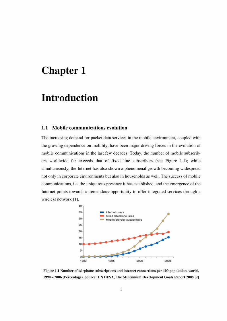
Figure 1.1 Number of telephone subscriptions and internet connections per 100 population,
world, 1990 – 2006 (Percentage). ............................................................................................... 1
Figure 1.2 Peak data rate evolution for WCDMA. ..................................................................... 6
Figure 2.1 The Complete Buffer Partitioning scheme for two traffic classes ............................ 16
Figure 2.2 Complete Buffer Sharing (CBS) implements FIFO with Drop-Tail .......................... 16
Figure 2.3 Pushout replacement mechanisms: LIFD, FIFD and random. .................................. 17
Figure 2.4 Partial Buffer Sharing (PBS) scheme. ...................................................................... 18
Figure 2.5 Precedence queuing or HOL priorities. .................................................................. 20
Figure 2.6 Typical locations of QoS management (RRM) functions in UTRA ......................... 37
Figure 3.1 UMTS/HSDPA system architecture ........................................................................ 45
Figure 3.2 HS-DSCH Protocol architecture ............................................................................. 48
Figure 3.3 UE side MAC-hs Architecture (details) ................................................................. 50
Figure 3.4 Detailed Node B MAC-hs architecture with functional entities ............................... 51
Figure 3.5 The new channels introduced in release 5 for HSDPA operation ............................. 52
Figure 3.6 Code multiplexing example with two active users .................................................. 53
Figure 3.7 HS-SCCH and HS-DSCH timing relationship ......................................................... 54
Figure 3.8 HS-DPCCH channel structure ................................................................................ 55
Figure 3.9 Terminal timing with respect to one HARQ process ............................................... 56
Figure 3.10 HSDPA User plane protocol stack ......................................................................... 57
Figure 4.1 A multimedia session with multiple flows of diverse media: video, voice and data. . 62
Figure 4.2 The Time-Space Priority queuing mechanism ......................................................... 63
Figure 4.3 States denoting the head-of-line status represented by p and q in the TSP model ..... 67
Figure 4.4 A section of the state space for the Continuous Time Markov Chain derived for TSP
investigation ............................................................................................................................ 68
Figure 4.5 NRT total loss probability (blocking and dropping) Vs R for λrt = 2, 12, and 18 ...... 75
List of figures
x
Figure 4.6 NRT mean queue length Vs R for λrt = 2, 12, and 18 .............................................. 76
Figure 4.7 NRT mean delay Vs R for λrt = 2, 12, and 18 ........................................................... 76
Figure 4.8 RT loss (blocking) probability Vs R for λrt = 2, 12, and 18 ...................................... 78
Figure 4.9 RT mean queue length Vs R for λrt = 2, 12, and 18 .................................................. 78
Figure 4.10 RT mean delay Vs R for λrt = 2, 12, and 18 ........................................................... 78
Figure 4.11 NRT loss Vs R for λnrt = 2, 6, and 9 and µnrt = 10 ............................................... 80
Figure 4.12 NRT mean queue length Vs R for λnrt = 2, 6, and 9 and µnrt = 10 ........................ 80
Figure 4.13 Mean NRT delay Vs R for λnrt = 2, 6, and 9 and µnrt = 10.................................... 80
Figure 4.14 RT loss Vs R for λnrt = 2, 6, and 9 and µnrt = 10 .................................................. 81
Figure 4.15 RT mean queue length Vs R for λnrt = 2, 6, and 9 and µnrt = 10 ........................... 82
Figure 4.16 Mean RT delay Vs R for λnrt = 2, 6, and 9 and µnrt = 10 ..................................... 82
Figure 4.17 WGoS Vs R for λrt = 2......................................................................................... 83
Figure 4.18 WGoS Vs R for λrt = 12, and 18 ........................................................................... 84
Figure 4.19 WGoS Vs R for λnrt = 2, 6, and 9 ......................................................................... 84
Figure 4.20 Simplified diagram of proposed optimization engine for semi real-time optimization
of the time space priority buffer threshold for HSDPA user session multimedia QoS control .... 85
Figure 4.21 Simplified model for investigating performance of the priority queuing mechanisms
for mobile radio access network downlink end-user multimedia traffic ..................................... 87
Figure 4.22 Mean RT delay vs. fraction of NRT arrivals in concurrent RT and NRT traffic for
TSP, CBP, PBS, CBS queuing ................................................................................................. 93
Figure 4.23 RT packet loss probability vs. fraction of NRT arrivals in concurrent RT and NRT
traffic for TSP, CBP, PBS, CBS queuing schemes ................................................................... 93
Figure 4.24 NRT packet loss probability vs. fraction of NRT arrivals in concurrent RT and
NRT traffic for TSP, CBP, PBS, CBS queuing schemes ........................................................... 94
Figure 4.25 Overall packet loss probability vs. fraction of NRT arrivals in concurrent RT and
NRT traffic for TSP, CBP, PBS, CBS queuing schemes ........................................................... 95
Figure 5.1 Logical hierarchy of UE1 multiplexed RT and NRT MAC-d flows’ in Node B MAC-
hs .......................................................................................................................................... 101
Figure 5.2 MAC-hs PDU structure ........................................................................................ 102
Figure 5.3 VoIP loss Vs FTP download rate in UE with multimedia traffic ............................ 108
List of figures
xi
Figure 5.4 VoIP mean delay Vs FTP download rate in UE with multimedia traffic ................. 109
Figure 5.5 FTP loss Vs FTP download rate in UE with multimedia traffic .............................. 110
Figure 5.6 FTP mean delay Vs FTP download rate in UE with multimedia traffic .................. 111
Figure 6.1 HSDPA flow control on the Iub interface. ............................................................. 115
Figure 6.2 HSDPA Iub interface flow control signalling procedure between RNC and Node B
.............................................................................................................................................. 116
Figure 6.3 Retransmission mechanisms in UMTS HSDPA for TCP based flows .................. 117
Figure 6.4 HSDPA RAN with E-TSP buffer management utilizing the proposed credit allocation
algorithm for per UE multi-flow Iub flow control ................................................................... 118
Figure 6.5 End-to-end HSDPA simulation set up .................................................................. 122
Figure 6.6 End-to-end NRT throughput at multimedia test UE with Complete Buffer Sharing for
1, 5, 10, 20 and 30 users utilizing the HSDPA shared channel ............................................... 125
Figure 6.7 End-to-end NRT throughput at multimedia test UE with TSP buffer management for
1, 5, 10, 20 and 30 users utilizing the HSDPA shared channel ............................................... 125
Figure 6.8 End-to-end NRT throughput at multimedia test UE with E-TSP buffer management
for 1, 5, 10, 20 and 30 users utilizing the HSDPA shared channel .......................................... 126
Figure 6.9 Average end-to-end NRT throughput at test UE Vs no. of users (CBS, TSP and E-
TSP) ...................................................................................................................................... 127
Figure 6.10 CBS VoIP UTRAN delay in test UE during multi-flow session ( 1, 5, 10, 20 and 30
users) ..................................................................................................................................... 128
Figure 6.11 TSP VoIP UTRAN delay in test UE during multi-flow session. Identical results were
obtained for E-TSP in all cases .............................................................................................. 130
Figure 6.12 Average UTRAN VoIP PDU delay at test UE Vs no. of users (CBS, TSP and E-
TSP) ...................................................................................................................................... 131
Figure 6.13 Average end-to-end VoIP PDU delay at test UE Vs number of users in cell.
Results given for CBS (left), TSP (center) and E-TSP ........................................................... 132
Figure 7.1 TSP BM with dynamic time priority switching (D-TSP) ....................................... 137
Figure 7.2 UE 1 NRT throughput for VoIP delay budget settings when utilizing the channel
alone ..................................................................................................................................... 144
Figure 7.3 UE 1 NRT throughput for VoIP delay budget settings with 5 users sharing channel
.............................................................................................................................................. 144
Figure 7.4 UE 1 NRT throughput for VoIP delay budget settings with 10 users sharing channel
.............................................................................................................................................. 145
List of figures
xii
Figure 7.5 UE 1 NRT throughput for various VoIP delay budget settings with 20 channel users
.............................................................................................................................................. 145
Figure 7.6 UE 1 NRT throughput for various VoIP delay budget settings with 30 channel users
.............................................................................................................................................. 146
Figure 7.7 UE 1 NRT throughput for VoIP delay budget settings with 50 users sharing channel
.............................................................................................................................................. 146
Figure 7.8 VoIP PDU Discarded in the MAC-hs for UE 1 ...................................................... 147
Figure 7.9 UE 1 HSDPA channel utilization for the delay budget settings .............................. 148
Figure 7.10 End-to-end NRT throughput of UE1 for TSP, D-TSP (δ = 8, 16, 24, and 32
respectively) .......................................................................................................................... 151
Figure 7.11 RT PDU discard ratio vs. number of users ........................................................... 153
Figure 7.12 RT inter-packet playout delay for all E-TSP scenarios. ...................................... 154
Figure 7.13 RT inter-packet playout delay for D-TSP δ= 24. .............................................. 155
Figure 7.14 RT inter- packet playout delay for D-TSP δ= 32. ............................................... 156
Figure B.1 Traffic source node model with RT and NRT source modules. ………….. ………188
Figure B.2 UTRAN Node model implementation ................................................................. 189
Figure B.3 RNC process model with RLC AM ARQ protocol ............................................... 190
Figure B.4 Node B process model implementation ................................................................. 191
Figure B.5 UE receiver node model implementation .............................................................. 193
List of tables
xiii
List of Tables
Table 2.1 Delay and loss priority assignment matrix .............................................................. 29
Table 2.2 UMTS QoS classes .................................................................................................. 36
Table 3.1 Comparison of fundamental properties of DCH and HS-DSCH ............................... 48
Table 4.1 Forward transitions from state X = (r, n, p, q) showing conditions and transition rates
................................................................................................................................................ 70
Table 4.2 Reverse transitions from state X = (r, n, p, q) showing conditions and transition rates 70
Table 4.3 Values of default parameters used in analytical models for comparative performance
evaluation of the priority queuing schemes............................................................................... 91
Table 5.1 Assumed AMC schemes and equivalent instantaneous bit rates per TTI ................ 105
Table 5.2 HSDPA simulation parameters ............................................................................. 106
Table 5.3 Multimedia UE MAC-hs buffer parameters for simulation study............................ 107
Table 6.1 Summary of assumed simulation parameters .......................................................... 123
Table 7.1 HSDPA Simulation parameters .............................................................................. 142
Table A.1 Validation of MOSEL results:- NRT loss (λRT = 2) ................................................ 172
Table A.2 Validation of MOSEL results:- RT loss (λRT = 2) .................................................. 173
Table A.3 Validation of MOSEL results:- NRT delay (λRT = 2) ............................................ 173
Table A.4 Validation of MOSEL results:- RT delay (λRT = 2) ............................................... 173
Table A.5 Validation of MOSEL results:- RT mean queue length (λRT = 2) .......................... 174
Table A.6 Validation of MOSEL results:- NRT mean queue length (λRT = 2) ...................... 174
Table A.7 Validation of MOSEL results:- NRT loss (λRT = 12) ............................................. 174
Table A.8 Validation of MOSEL results:- RT loss (λRT = 12)................................................ 175
Table A.9 Validation of MOSEL results:- NRT delay (λRT = 12) ........................................... 175
Table A.10 Validation of MOSEL results:- RT delay (λRT = 12) ............................................ 175
Table A.11 Validation of MOSEL results:- RT mean queue length (λRT =12) ........................ 176
Table A.12 Validation of MOSEL results:- NRT mean queue length (λRT =12) ..................... 176
List of tables
xiv
Table A.13 Validation of MOSEL results:- NRT loss (λRT = 18) ............................................ 176
Table A.14 Validation of MOSEL results:- RT loss (λRT = 18) ............................................... 177
Table A.15 Validation of MOSEL results:- NRT delay (λRT = 18) ......................................... 177
Table A.16 Validation of MOSEL results:- RT delay (λRT = 18) ............................................ 177
Table A.17 Validation of MOSEL results:- RT mean queue length (λRT =18) ........................ 178
Table A.18 Validation of MOSEL results:- NRT mean queue length (λRT =18) ..................... 178
Table A.19 Validation of MOSEL results:- NRT loss (λNRT = 2) ........................................... 179
Table A.20 Validation of MOSEL results:- RT loss (λNRT = 2) ............................................. 179
Table A.21 Validation of MOSEL results:- NRT delay (λNRT = 2) ......................................... 180
Table A.22 Validation of MOSEL results:- RT delay (λNRT = 2) ........................................... 180
Table A.23 Validation of MOSEL results:- RT mean queue length (λNRT = 2) ....................... 180
Table A.24 Validation of MOSEL results:- NRT mean queue length (λNRT = 2) .................... 181
Table A.25 Validation of MOSEL results:- NRT loss (λNRT = 6) ........................................... 181
Table A.26 Validation of MOSEL results:- RT loss (λNRT = 6) ............................................... 181
Table A.27 Validation of MOSEL results:- NRT delay (λNRT = 6) .......................................... 182
Table A.28 Validation of MOSEL results:- RT delay (λNRT = 6) ............................................ 182
Table A.29 Validation of MOSEL results:- RT mean queue length (λNRT = 6) ....................... 182
Table A.30 Validation of MOSEL results:- NRT mean queue length (λNRT = 6) .................... 183
Table A.31 Validation of MOSEL results:- NRT loss (λNRT = 9) ........................................... 183
Table A.32 Validation of MOSEL results:- RT loss (λNRT = 9) .............................................. 183
Table A.33 Validation of MOSEL results:- NRT delay (λNRT = 9) .......................................... 184
Table A.34 Validation of MOSEL results:- RT delay (λNRT = 9) ............................................ 184
Table A.35 Validation of MOSEL results:- RT mean queue length (λNRT = 9) ....................... 184
Table A.36 Validation of MOSEL results:- NRT mean queue length (λNRT = 9) .................... 185
Table B.1 list of implemented key Node B process functions ................................................ 191
Abbreviations
xv
Abbreviations
1G First Generation
2G Second Generation
3G Third Generation
3GPP Third Generation Partnership Project
AC Admission Control
AM Acknowledged Mode
AMC Adaptive Modulation and Coding
AMPS Advanced Mobile Phone Service
ARQ Automatic repeat reQuest
ATM Asynchronous Transfer Mode
BAC Buffer Admission Control
BLER Block Error Rate
BMA Buffer Management Algorithm
BSC Base Station Controller
CBP Complete Buffer Partitioning
CBR Constant Bit Rate
CBS Complete Buffer Sharing
CDMA Code Division Multiple Access
CLP Cell Loss Priority
CN Core Network
CQI Channel Quality Indicator
CRC Cyclic Redundancy Check
CRNC Controlling Radio Network Controller
CTMC Continuous Time Markov Chain
DCH Dedicated Channel
DSCH Downlink Shared Channel
DT Discard Timer
D-TSP Dynamic Time-Space Priority
ECSD Enhanced Circuit Switched Data
EDGE Enhanced Data for Global Evolution
EGPRS Enhanced GPRS
ETSI European Telecommunications Standards Institute
E-TSP Enhanced Time-Space Priority
FACH Forward Access Channel
FDD Frequency Division Duplex
FIFD First-in-first-drop
FIFO First-in-first-out
Abbreviations
xvi
FP Frame Protocol
FTP File Transfer Protocol
GBR Guaranteed Bit Rate
GGSN Gateway GPRS Support Node
GPRS General Packet Radio Service
GSM Global System for Mobile Communication
HARQ Hybrid Automatic Repeat reQuest
HOL Head-of-the-Line
HSCSD High Speed Circuit Switched Data
HSDPA High Speed Downlink Packet Access
HS-DPCCH High Speed Dedicated Physical Control Channel
HS-DSCH High Speed Downlink Shared Channel
HSPA High Speed Packet Access
HS-SCCH High-Speed Shared Control Channel
HSUPA High Speed Uplink Packet Access
IMT-2000 International Mobile Telecommunications 2000
IP Internet Protocol
IPv4 Internet Protocol version 4
IPv6 Internet Protocol version 6
ITU The International Telecommunication Union
LIFD Last-in-first-drop
LTE Long-Term Evolution
MAC Medium Access Control
MAC-hs MAC high speed
ME Mobile Equipment
MOSEL MOdelling Specification and Evaluation Language
MSC Mobile Switching Centre
NRT Non-real-time
PBS Partial Buffer Sharing
PDC Personal Digital Cellular
PDCP Packet Data Convergence Protocol
PDU Protocol Data Unit
PHY Physical Layer
PO Pushout
PS Packet Scheduling
QAM Quadrature Amplitude Modulation
QoS Quality of Service
QPSK Quaternary Phase Shift Keying
R99 Release 99
RAB Radio Access Bearer
Abbreviations
xvii
RAN Radio Access Network
RLC Radio Link Control
RNC Radio Network Controller
RNS Radio Network Subsystem
RRC Radio Resource Control
RRM Radio Resource Management
RT Real-time
SDU Service Data Units
SF Spreading Factor
SGSN Serving GPRS Support Node
SINR Signal-to-Interference-plus-Noise-Ratio
SMS Short Messaging Services
SPI Service Priority Indicator
SRNC Serving Radio Network Controller
TC Traffic Class
TCP Transmission Control Protocol
TDD Time Division Duplex
TDMA Time Division Multiple Access
TF Transport Format
TFCI Transport Format Combination Identification
TM Transparent Mode
ToS Type of Service
TSN Transmission Sequence Number
TSP Time-Space Priority
TTI Transmission Time Interval
UDP User Datagram Protocol
UE User Equipment
UM Unacknowledged Mode
UMTS Universal Mobile Telecommunications System
USIM UMTS Subscriber Identity Module
UTRA Universal Terrestrial Radio Access
UTRAN UMTS Terrestrial Radio Access Network
VBR Variable Bit Rate
VoIP Voice over IP
WCDMA Wideband Code Division Multiple Access
WGoS Weighted Grade of Service
1
Chapter 1
Introduction
1.1 Mobile communications evolution
The increasing demand for packet data services in the mobile environment, coupled with
the growing dependence on mobility, have been major driving forces in the evolution of
mobile communications in the last few decades. Today, the number of mobile subscrib-
ers worldwide far exceeds that of fixed line subscribers (see Figure 1.1); while
simultaneously, the Internet has also shown a phenomenal growth becoming widespread
not only in corporate environments but also in households as well. The success of mobile
communications, i.e. the ubiquitous presence it has established, and the emergence of the
Internet points towards a tremendous opportunity to offer integrated services through a
wireless network [1].
Figure 1.1 Number of telephone subscriptions and internet connections per 100 population, world,
1990 – 2006 (Percentage). Source: UN DESA, The Millennium Development Goals Report 2008 [2]
Chapter 1: Introduction 2
2
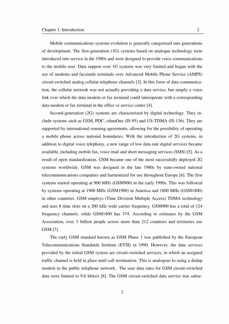
Mobile communications systems evolution is generally categorized into generations
of development. The first-generation (1G) systems based on analogue technology were
introduced into service in the 1980s and were designed to provide voice communications
to the mobile user. Data support over 1G systems was very limited and began with the
use of modems and facsimile terminals over Advanced Mobile Phone Service (AMPS)
circuit-switched analog cellular telephone channels [3]. In this form of data communica-
tion, the cellular network was not actually providing a data service, but simply a voice
link over which the data modem or fax terminal could interoperate with a corresponding
data modem or fax terminal in the office or service center [4].
Second-generation (2G) systems are characterized by digital technology. They in-
clude systems such as GSM, PDC, cdmaOne (IS-95) and US-TDMA (IS-136). They are
supported by international roaming agreements, allowing for the possibility of operating
a mobile phone across national boundaries. With the introduction of 2G systems, in
addition to digital voice telephony, a new range of low data rate digital services became
available, including mobile fax, voice mail and short messaging services (SMS) [5]. As a
result of open standardization, GSM became one of the most successfully deployed 2G
systems worldwide. GSM was designed in the late 1980s by state-owned national
telecommunications companies and harmonized for use throughout Europe [6]. The first
systems started operating at 900 MHz (GSM900) in the early 1990s. This was followed
by systems operating at 1900 MHz (GSM1900) in America and 1800 MHz (GSM1800)
in other countries. GSM employs (Time Division Multiple Access) TDMA technology
and uses 8 time slots on a 200 kHz wide carrier frequency. GSM900 has a total of 124
frequency channels, while GSM1800 has 374. According to estimates by the GSM
Association, over 3 billion people across more than 212 countries and territories use
GSM [7].
The early GSM standard known as GSM Phase 1 was published by the European
Telecommunications Standards Institute (ETSI) in 1990. However, the data services
provided by the initial GSM system are circuit-switched services, in which an assigned
traffic channel is held in place until call termination. This is analogous to using a dialup
modem in the public telephone network. The user data rates for GSM circuit-switched
data were limited to 9.6 kbits/s [8]. The GSM circuit-switched data service was subse-
Chapter 1: Introduction 3
3
quently enhanced with High Speed Circuit Switched Data (HSCSD), specified as part of
GSM Phase 2+ in 1996. HSCSD [9] allowed bundling of several time slots in addition to
channel coding adaptation to the radio channel quality (i.e. 9.6 kbits/s per time slot or
14.4 kbits/s per time slot). Thus, HSCSD enables up to 57.6 kbits/s with four 14.4 kbits/s
time slots; and, by combining eight GSM time slots the capacity can be increased to 115
kbits/s. In practice, the maximum data rate is limited to 64 kbits/s owing to limitations in
the GSM network [10].
Soon after the first GSM networks became operational in the early 90s, it became
evident that the circuit-switched bearer services were not particularly well suited for
certain types of applications with “bursty” data traffic. The circuit-switched data services
were not cost-effective for the customer using the service for connections to the Internet
or corporate networks. Similarly, from the service provider’s perspective, the use of
circuit-switched connections for carrying bursty traffic did not make efficient use of
cellular network capacity. At the same time, customer demand for higher-rate data grew
steadily as new software applications for mobile users entered the marketplace. These
prompted the development of General Packet Radio Service (GPRS) [11], [12], [13],
[14], as part of the GSM Phase 2+ specification which was approved by 1997. Signifi-
cantly, unlike GSM and HSCSD which are circuit-switched, GPRS is a packet-switched
system. The aim of GPRS is to provide Internet-type services to mobile users, bringing
together the convergence of IP and Mobility. GPRS which can be considered as a
stepping stone between GSM and third-generation UMTS is widely regarded as a 2.5G
system.
GPRS makes use of the same radio interface as GSM but introduces a packet
switched domain into the Core Network (CN) of GSM. The GPRS protocol dynamically
allocates a time slot to various users so that they can alternately transmit data. With
GPRS, a user is continuously connected but may only be charged for the data that is
transported over the network. GPRS uses coding schemes to adapt channel coding to the
quality of the radio channel (CS1: 9.05 kbit/s, CS2: 13.4 kbit/s, CS3: 15.6 kbit/s, CS4:
21.4 kbit/s) and is able to use several time slots per connection. GPRS can allow a
maximum 171.2 kbit/s (CS4 with 8 time-slots) to be achieved. However, under more
Chapter 1: Introduction 4
4
realistic conditions (i.e. loaded network) the average user throughput of GPRS could
range around 30 – 40 kbit/s [6].
Further evolution of cellular data services includes Enhanced Data for Global Evo-
lution (EDGE), which builds upon the GPRS architecture. EDGE was introduced to
meet the need for higher data rates for an expanding menu of service such as multimedia
transmission which were beyond the capacity of deployed GSM/GPRS networks. In
response to this market demand, the ETSI defined a new family of data services, built
upon the existing structure of GPRS. This new family of data services was initially
named Enhanced Data Rates for GSM Evolution, and subsequently renamed Enhanced
Data for Global Evolution. While the primary motivation for the EDGE development
was enhancement of data services in GSM/GPRS networks, EDGE can also be intro-
duced into networks built to the IS-136 (US Digital Cellular) standard [15]. In Europe,
EDGE is considered a 2.5 generation (2.5G) standard, providing a transition between 2G
and 3G systems. As is the case with GPRS, a GSM network operator requires no new
license to implement EDGE services in its network, since the 200-kHz RF channel
organization of conventional GSM is reused with a different organization of logical
channels within each RF channel.
EDGE enhances data service performance over GPRS in two ways. First, it replac-
es the GMSK radio link modulation used in GSM with an 8-PSK modulation scheme
capable of tripling the data rate on a single radio channel. Second, EDGE provides more
reliable transmission of data using a link adaption technique, which dynamically chooses
a modulation and coding scheme (MCS) in accordance with the current transmission
conditions on the radio channel. The EDGE link adaptation mechanism is an enhanced
version of the link adaptation mechanism used in GPRS [16], [17]. EDGE provides two
forms of enhanced data service for GSM networks – Enhanced Circuit Switched Data
(ECSD) for circuit switched services and Enhanced GPRS (EGPRS) for packet switched
services. In each form of EDGE data service, there are provisions for combining logical
channels (time slots) in the GSM transmission format to provide a wide menu of achiev-
able data rates. The ETSI Phase 1 EDGE standard considers both ECSD and EGPRS
services, with data rates of up to 38.4 kbit/s/time-slot and 60 kbit/s/time-slot respective-
ly. Higher data rates can be achieved by combining logical channels; so for example, a
Chapter 1: Introduction 5
5
64 kbit/s service could be achieved by combining two ECSD channels. Rates over 400
kbit/s can be achieved for EGPRS [18].
Following the success of 2G systems worldwide, third-generation (3G) systems
were introduced to provide global mobility with wide range of services including
telephony, paging, messaging, Internet and broadband data. The International Telecom-
munication Union (ITU) started the process of defining the standard for third generation
systems, referred to as International Mobile Telecommunications 2000 (IMT-2000). In
Europe, the 3G system was known as the Universal Mobile Telecommunications System
(UMTS) and ETSI was responsible for its standardization process. In 1998 Third Gener-
ation Partnership Project (3GPP) was formed to continue the technical specification
work for UMTS. In January 1998, ETSI selected Wideband Code Division Multiple
Access (WCDMA) as the UMTS air interface [19]. Within 3GPP, WCDMA is called
Universal Terrestrial Radio Access (UTRA) Frequency Division Duplex (FDD) and
Time Division Duplex (TDD), the term WCDMA being used to cover both FDD and
TDD operations [20]. UMTS WCDMA is a Direct Sequence CDMA system where user
data is multiplied with quasi-random bits (called chips) derived from WCDMA Spread-
ing codes. A chip rate of 3.84 Mcps is used which leads to a carrier bandwidth of
approximately 5 MHz. While UMTS required a new spectrum for the WCDMA air
interface, and introduced new radio network architecture, the core network infrastructure
was the same as that of GSM/GPRS. UMTS enables both circuit-switched and packet-
switched services.
The first full set of UMTS specifications was completed at the end of 1999, called
Release 99 (R99), while the first commercial network was launched in Japan in 2001 and
commercial use in Europe began in 2003. 3GPP specified important evolution steps on
top of WCDMA known collectively as High Speed Packet Access (HSPA) for downlink
in Release 5 and Uplink in Release 6. The Downlink solution, High Speed Downlink
Packet Access (HSDPA) was commercially deployed in 2005 and the Uplink counter-
part, High Speed Uplink Packet Access (HSUPA), during 2007 [20]. HSDPA is also
referred to as a 3.5G wireless technology.
The work in this thesis focuses on multimedia traffic control and optimization in
WCDMA HSDPA-UMTS networks to enhance end-to-end communication. UMTS R99
Chapter 1: Introduction 6
6
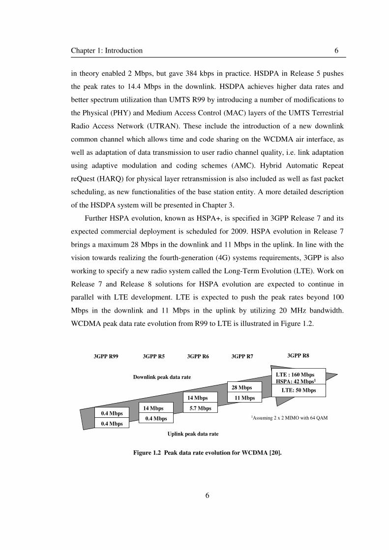
in theory enabled 2 Mbps, but gave 384 kbps in practice. HSDPA in Release 5 pushes
the peak rates to 14.4 Mbps in the downlink. HSDPA achieves higher data rates and
better spectrum utilization than UMTS R99 by introducing a number of modifications to
the Physical (PHY) and Medium Access Control (MAC) layers of the UMTS Terrestrial
Radio Access Network (UTRAN). These include the introduction of a new downlink
common channel which allows time and code sharing on the WCDMA air interface, as
well as adaptation of data transmission to user radio channel quality, i.e. link adaptation
using adaptive modulation and coding schemes (AMC). Hybrid Automatic Repeat
reQuest (HARQ) for physical layer retransmission is also included as well as fast packet
scheduling, as new functionalities of the base station entity. A more detailed description
of the HSDPA system will be presented in Chapter 3.
Further HSPA evolution, known as HSPA+, is specified in 3GPP Release 7 and its
expected commercial deployment is scheduled for 2009. HSPA evolution in Release 7
brings a maximum 28 Mbps in the downlink and 11 Mbps in the uplink. In line with the
vision towards realizing the fourth-generation (4G) systems requirements, 3GPP is also
working to specify a new radio system called the Long-Term Evolution (LTE). Work on
Release 7 and Release 8 solutions for HSPA evolution are expected to continue in
parallel with LTE development. LTE is expected to push the peak rates beyond 100
Mbps in the downlink and 11 Mbps in the uplink by utilizing 20 MHz bandwidth.
WCDMA peak data rate evolution from R99 to LTE is illustrated in Figure 1.2.
0.4 Mbps
0.4 Mbps
14 Mbps
0.4 Mbps
14 Mbps
5.7 Mbps
28 Mbps
11 Mbps
LTE : 160 Mbps
HSPA: 42 Mbps1
LTE: 50 Mbps
3GPP R99 3GPP R5 3GPP R6 3GPP R7
Downlink peak data rate
Uplink peak data rate
1Assuming 2 x 2 MIMO with 64 QAM
3GPP R8
Figure 1.2 Peak data rate evolution for WCDMA [20].
Chapter 1: Introduction 7
7
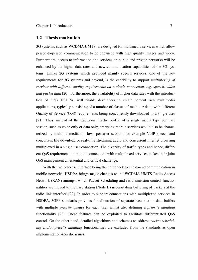
1.2 Thesis motivation
3G systems, such as WCDMA UMTS, are designed for multimedia services which allow
person-to-person communication to be enhanced with high quality images and video.
Furthermore, access to information and services on public and private networks will be
enhanced by the higher data rates and new communication capabilities of the 3G sys-
tems. Unlike 2G systems which provided mainly speech services, one of the key
requirements for 3G systems and beyond, is the capability to support multiplexing of
services with different quality requirements on a single connection, e.g. speech, video
and packet data [20]. Furthermore, the availability of higher data rates with the introduc-
tion of 3.5G HSDPA, will enable developers to create content rich multimedia
applications, typically consisting of a number of classes of media or data, with different
Quality of Service (QoS) requirements being concurrently downloaded to a single user
[21]. Thus, instead of the traditional traffic profile of a single media type per user
session, such as voice only or data only, emerging mobile services would also be charac-
terized by multiple media or flows per user session; for example VoIP speech and
concurrent file download or real-time streaming audio and concurrent Internet browsing
multiplexed in a single user connection. The diversity of traffic types and hence, differ-
ent QoS requirements in mobile connections with multiplexed services makes their joint
QoS management an essential and critical challenge.
With the radio access interface being the bottleneck to end-to-end communication in
mobile networks, HSDPA brings major changes to the WCDMA UMTS Radio Access
Network (RAN) amongst which Packet Scheduling and retransmission control functio-
nalities are moved to the base station (Node B) necessitating buffering of packets at the
radio link interface [22]. In order to support connections with multiplexed services in
HSDPA, 3GPP standards provides for allocation of separate base station data buffers
with multiple priority queues for each user whilst also defining a priority handling
functionality [23]. These features can be exploited to facilitate differentiated QoS
control. On the other hand, detailed algorithms and schemes to address packet schedul-
ing and/or priority handling functionalities are excluded from the standards as open
implementation-specific issues.
Chapter 1: Introduction 8
8
From the subscriber perspective, end-to-end QoS provisioning is a critical factor for
high-quality multiplexed services on mobile systems. From the mobile operator perspec-
tive, efficient network resource and radio link utilization while providing the end-user
multiplexed services are crucial to enhancing capacity and increased revenue. These
objectives can be met through control, management and QoS optimization of the various
flows comprising the multiplexed services connection; and a very effective and viable
solution which can readily employ existing 3GPP standardized mechanisms, is to
incorporate buffer management strategies at the bottleneck radio link interface.
Hence, in a nutshell, the work in this thesis is motivated by the need for solutions to
address the problem of differentiated control and Quality of Service optimization of
mobile multimedia traffic with multiplexed services in 3.5G networks in order to en-
hance end-user communications whist allowing efficient utilization of radio link and
network resources. The thesis proposes novel buffer management schemes for the
control, management and performance optimization of the differentiated multiplexed
flows in the same multimedia session of a HSDPA mobile user.
1.3 Aim and objectives
The main aim of the project is to propose solutions that address the problem of opti-
mized Quality of Service support for improved end-to-end performance of multimedia
traffic within a user session and efficient resource utilization in 3.5G mobile systems
using radio link buffer management.
Thus the objectives of the thesis are as follows:
1. To survey, study and understand existing queuing and buffer management
solutions in order to analyze their applicability to QoS optimization of mul-
timedia traffic with diverse classes of flows.
2. To develop and investigate multi-class (priority) queuing systems that can
fulfill the requirement for joint QoS control of concurrent diverse flows
within an end-user multimedia session in 3.5G mobile systems.
3. To evaluate the performance of the viable queuing systems using analytical
and simulation models in order to gain further insight through in-depth ana-
lyses.
Chapter 1: Introduction 9
9
4. To research, study and explore the options from 3GPP (UMTS/HSDPA)
standard specifications which can be employed in the design of novel solu-
tions for QoS optimization of the emerging multimedia services.
5. To develop new buffer management algorithms based on the viable queuing
models and compatible with 3GPP standards to address the problem of mul-
timedia traffic QoS support with efficient resource utilization at the
‘bottleneck’ radio interface of the 3.5G network.
6. To evaluate the impact of the new buffer management algorithms on end-to-
end communication and system performance using dynamic system-level
HSDPA simulation.
1.4 Thesis contribution
The main contributions of this thesis are as follows:
1. A novel queuing system known as Time-Space Priority (TSP) queuing is
proposed as the core concept for the buffer management-based multimedia
QoS control schemes for multiplexed flows in a downlink mobile connec-
tion. With TSP, the multiplexed flows are classed into real-time (RT) and
non-real-time (NRT) where RT packets enjoy time (transmission) priority
but with a restricted buffer access to control the delay and jitter, while delay-
tolerant NRT packets are given unrestricted buffer access i.e. space priority
to minimize loss. Thus, unlike most existing priority queuing schemes where
only a single priority criteria is used for differentiated flows i.e. space priori-
ty or time priority, TSP combines both time and space priorities in a single
queue discipline to suit the diverse QoS requirements of RT and NRT
classes.
2. Stochastic-Analytic models are developed for Time-Space Priority queuing,
providing an effective tool for studying the TSP performance under a range
of traffic and system configurations, as well comparison of TSP with con-
ventional priority queuing schemes. (Chapter 4).
Chapter 1: Introduction 10
10
3. A TSP-based QoS optimization function to allow semi real-time optimiza-
tion of the radio link buffer is formulated and a conceptual framework for
integrating the function into mobile networks is presented. (Chapter 4).
4. A new buffer management scheme termed Enhanced Time-Space priority
(E-TSP) is proposed for HSDPA radio link buffer management of end-user
multimedia traffic with concurrent RT and NRT flows. In addition to basic
TSP queuing, E-TSP incorporates a novel credit-based flow control algo-
rithm designed to optimize radio link buffer queuing in response to the time-
varying radio link quality and downlink channel load. The flow control algo-
rithm mitigates buffer overflow thereby improving higher layer protocol
performance resulting in end-to-end QoS enhancement of the NRT flow in
the multiplexed traffic. E-TSP performance is evaluated via extensive sys-
tem-level HSDPA simulations. (Chapter 6).
5. The concept of dynamic time priority switching (between the multiplexed
flows) is introduced to time-space priority queuing. The idea is to exploit
any residual QoS (i.e. delay) tolerance of the RT packets in order to switch
time/transmission priority to NRT flow. This improves the fairness proper-
ties of TSP queuing resulting in enhanced end-to-end NRT throughput
without compromising the RT QoS requirements. Based on this idea, a new
Dynamic Time-Space priority (D-TSP) buffer management scheme is pro-
posed for HSDPA multimedia traffic QoS optimization in the base station
buffer. D-TSP performance is evaluated via extensive system-level HSDPA
simulations. (Chapter 7).
1.5 Thesis outline
The outline of the thesis organization is as follows:
Chapter 1: gives a brief introduction to mobile communications evolution, explains the
thesis motivation, the research aim and objectives and also outlines the main contribu-
tions of the thesis. A list of selected author’s publications in the literature through which
various aspects of the work in this thesis have been disseminated is also included.
Chapter 1: Introduction 11
11
Chapter 2: discusses buffer management and QoS control, providing a review of the
existing priority queuing/buffer management schemes and other relevant related works
in the open literature.
Chapter 3: provides description of the 3.5G HSDPA system in order to establish the
technological background to put the solutions proposed in this thesis into context.
Chapter 4: introduces the Time-Space priority (TSP) queuing concept together with
analytical model development using Markov chains. Performance analyses of TSP
queuing are presented here, and also comparative performance analyses of TSP queuing
with conventional priority queuing schemes are presented. A framework for TSP-based
buffer optimization to facilitate semi real-time adaptive QoS control of the multiplexed
flows in the HSDPA multimedia session also presented in this chapter.
Chapter 5: presents the TSP buffer management algorithm in HSDPA. TSP based
buffer management is also compared to conventional schemes via discrete event simula-
tion of HSDPA system.
Chapter 6: presents the E-TSP algorithm together with the performance evaluation of
E-TSP to investigate its impact on multimedia traffic end-to-end performance using
dynamic system-level HSDPA simulations.
Chapter 7: presents the D-TSP algorithm together with the performance evaluation of
D-TSP to investigate its impact on multimedia traffic end-to-end performance by means
of dynamic system-level HSDPA simulations.
Chapter 8: draws the main conclusions of the thesis work and discusses areas for
possible future investigation.
1.6 Author’s selected publications
Journal Papers
1. A. I. Zreikat, S.Y. Yerima, K. Al-Begain “Performance Evaluation and Re-
source Management of Hierarchical MACRO-/MICRO Cellular Networks
Using MOSEL-2” Wireless Personal Communications. Volume 44, Issue 2,
January 2008) Pages: 153 - 179 ISSN: 0929-6212.
2. K. Al-Begain, A. Dudin, A. Karzimirsky, S. Y. Yerima “ Investigation of
the M2/G2/1/ ∞, N Queue with Restricted Admission of Priority Customers
Chapter 1: Introduction 12
12
and its Application to HSDPA Mobile Systems” Computer Networks Jour-
nal (in press).
3. S. Y. Yerima and K. Al-Begain “Novel Radio Link Buffer Management
Schemes for End-user Multimedia Traffic in High Speed Downlink Packet
Access Networks” (Submitted to Wireless Personal Communications).
Book chapter Contributions
4. K. Al-Begain, S.Y. Yerima, A. Dudin, V. Mushko “Novel buffer Manage-
ment Scheme for Multimedia Traffic in HSDPA” Section in Packet
Scheduling and Congestion Control chapter of the COST 290 Action book.
(To be published as Springer Lecture Notes in Computer Science).
5. K. Al-Begain, S. Y. Yerima, B. AbuHaija “Packet Scheduling and Buffer
Management” contributed chapter in Handbook of HSDPA/HSUPA Tech-
nology. (To be published by CRC group Taylor and Francis, fall 2009).
Conference proceedings
6. S. Y. Yerima, K. Al-Begain, “Analysis of M2/M2/1/R, N Queuing model for
Multimedia over 3.5G Wireless Network Downlink” Proceedings of the Eu-
ropean Modeling Symposium (EMS 2006), London, U.K. pp 79-83, ISBN:
0-9516509—9/978-0-9516509-3-6, September 2006.
7. S. Y. Yerima, K. Al-Begain, “Buffer Management for Multimedia QoS
control over HSDPA Downlink” 21st IEEE International Conference on Ad-
vanced Information Networking and Applications (AINA 2007), Niagara
Falls, Ontario Canada. Volume 1, pp 912-917, ISBN: 0-7695-2647-3, May
2007.
8. S. Y. Yerima, K. Al-Begain, “An Enhanced Buffer Management Scheme
for Multimedia Traffic in HSDPA”. 1st IEEE International Conference on
Next Generation Mobile Applications, Services and Technologies
(NGMAST 2007) Cardiff, Wales. pp 292-297, ISBN- 0-7695-2878-3 Sep-
tember 12-14, 2007.
9. S. Y. Yerima, K. Al-Begain, “A Dynamic Buffer Management Scheme for
End-to-End QoS Enhancement of Multi-flow Services in HSDPA” 2nd
IEEE International Conference on Next Generation Mobile Applications,
Chapter 1: Introduction 13
13
Services and Technologies (NGMAST 2008) Cardiff, Wales, 15-17 Septem-
ber, 2008.
10. S. Y. Yerima, K. Al-Begain, “End-to-End QoS Enhancement of HSDPA
End-User Multi-flow Traffic Using RAN Buffer Management” 2nd
IFIP/IEEE International Conference on New Technologies, Mobility and Se-
curity, (NTMS 2008) Tangier, Morocco, 5-7 November, 2008.
11. S. Y. Yerima, K. Al-Begain, “Dynamic Buffer Management for Multime-
dia Services in 3.5G Wireless Networks” International Conference of
Wireless Networks, IAENG World Congress on Engineering 2009, 1-3 July
2009. (Accepted with nomination for best paper competition)
Workshop/Symposia proceedings
12. S. Y. Yerima, K. Al-Begain,“ Performance Modeling of a Novel Queuing
Model for Multimedia over 3.5G Downlink Using MOSEL-2” Proceedings
of the 7th
Annual Postgraduate Symposium on The Convergence of Tele-
communications, Networking & Broadcasting (PG Net 2006), Liverpool,
U.K. pp 254-259, ISBN 1-9025-6013-9, June 2006.
13. S. Y. Yerima, K. Al-Begain “Buffer Management for Downlink Multime-
dia QoS Control in HSDPA Radio Access Networks” Proceedings of the 1st
Faculty of Advanced Tech. Workshop, University of Glamorgan, U.K. pp70-
74, ISBN: 978-1-84054-156-4 May 2007.
14. S. Y. Yerima, K. Al-Begain, “Performance Modeling of a Queue Man-
agement Scheme with Rate Control for HSDPA” Proceedings of the 8th
Annual Postgraduate Symposium on the Convergence of Telecommunica-
tions, Networking & Broadcasting (PG Net 2007), Liverpool, U.K., June
2007.
15. S. Y. Yerima, “Evaluating Active Buffer Management for HSDPA Multi-
flow Services Using OPNET” Proceedings of the 3rd Faculty of Advanced
Tech. Workshop, University of Glamorgan, U.K. pp 6-11, ISBN: 978-1-
84054-179-3 May 2008. (Won Faculty prize for best paper and the out-
standing presentation in the workshop).
14
Chapter 2
Buffer Management and Quality of
Service
2.1 Introduction
This chapter presents buffer management fundamentals from the viewpoint of Quality of
Service control. A review of the literature related to buffer management in both wireline
and wireless networks is presented. Most existing proposals fall either into space priority
or time priority buffer management, employing mechanisms to provide differentiated
loss treatment to multiple flows in the former, or differentiated delay treatment in the
latter.
The chapter also provides discussion on service differentiation and QoS mechan-
isms with respect to mobile networks, particularly UMTS/HSDPA, since the buffer
management schemes proposed in the thesis necessarily interact with these mechanisms.
Chapter 2: Buffer management and Quality of Service 15
2.2 Buffer management fundamentals
Buffer management is a fundamental technology to provide Quality of Service (QoS)
control mechanisms, by controlling the assignment of buffer resources among different
flows or flow aggregation according to certain policies [24]. Traditionally, buffer
management has been used in the Internet to allocate memory space and link resources
to various flows arriving at switches and routers; and because of its significant impact on
traffic end-to-end performance, several buffer management schemes have been proposed
in the literature. With the rapid growth of wireless Internet access and wireless packet-
switched multimedia services, buffer management is increasingly becoming an impor-
tant tool for QoS control in wireless access networks as well.
There are various ways of classifying buffer management schemes that can be found
in the literature but the most common ones include:
a) Classification by resource management i.e. how the buffer space as a resource
itself is shared amongst the different flows or services.
b) Classification by service differentiation i.e. according to way the different flows
are handled or prioritized, usually with preferential treatment depending on ser-
vice class in order to control a specific QoS parameter e.g. loss or delay.
c) Classification by granularity of priority handling i.e. implicit
(call/session/connection level priority handling) or explicit (flow level priority
handling).
2.2.1 Classification by resource management
From resource management viewpoint, buffer management schemes can be categorized
into three classes namely, complete partitioning policy based (CBP), complete sharing
policy based (CBS) and partial buffer sharing (PBS) policy based [25, 26].
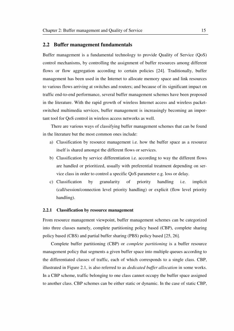
Complete buffer partitioning (CBP) or complete partitioning is a buffer resource
management policy that segments a given buffer space into multiple queues according to
the differentiated classes of traffic, each of which corresponds to a single class. CBP,
illustrated in Figure 2.1, is also referred to as dedicated buffer allocation in some works.
In a CBP scheme, traffic belonging to one class cannot occupy the buffer space assigned
to another class. CBP schemes can be either static or dynamic. In the case of static CBP,
Chapter 2: Buffer management and Quality of Service 16
the assigned buffer space is not adjusted with traffic load variation. On the other hand,
dynamic CBP extends the static CBP by allowing buffer allocation adjustment according
to changing traffic load. Because of the capability to adjust buffer allocation to traffic
load, dynamic CBP schemes generally improve buffer utilization and reduce overall
packet loss rate compared to static CBP.
CBP
Figure 2.1 The Complete Buffer Partitioning scheme for two traffic classes
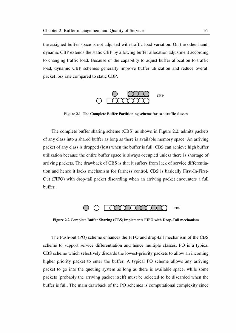
The complete buffer sharing scheme (CBS) as shown in Figure 2.2, admits packets
of any class into a shared buffer as long as there is available memory space. An arriving
packet of any class is dropped (lost) when the buffer is full. CBS can achieve high buffer
utilization because the entire buffer space is always occupied unless there is shortage of
arriving packets. The drawback of CBS is that it suffers from lack of service differentia-
tion and hence it lacks mechanism for fairness control. CBS is basically First-In-First-
Out (FIFO) with drop-tail packet discarding when an arriving packet encounters a full
buffer.
CBS
Figure 2.2 Complete Buffer Sharing (CBS) implements FIFO with Drop-Tail mechanism
The Push-out (PO) scheme enhances the FIFO and drop-tail mechanism of the CBS
scheme to support service differentiation and hence multiple classes. PO is a typical
CBS scheme which selectively discards the lowest-priority packets to allow an incoming
higher priority packet to enter the buffer. A typical PO scheme allows any arriving
packet to go into the queuing system as long as there is available space, while some
packets (probably the arriving packet itself) must be selected to be discarded when the
buffer is full. The main drawback of the PO schemes is computational complexity since

Chapter 2: Buffer management and Quality of Service 17
the lowest priority packet has to be ‘found’ before being overwritten by the higher
priority packet. The simplest PO mechanism is to remove the tail packet of the lowest
class when a packet needs to be discarded. This replacement strategy, which can be seen
in Figure 2.3, is known as the Last in First Drop (LIFD). Other PO replacement strate-
gies include the First in First Drop (FIFD) where the head packet of the lowest class is
discarded to make room for the arriving packet; and the Random replacement strategy
where a random packet of the lowest class is discarded in favour of the arriving packet.
Pushout
Pushout
Pushout
LIFD
FIFD
RANDOM
Figure 2.3 Pushout replacement mechanisms: LIFD, FIFD and random.
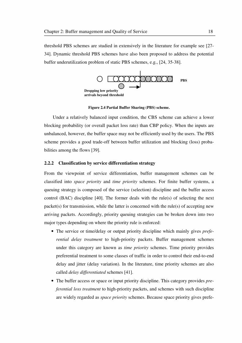
Partial buffer sharing (PBS), as illustrated in Figure 2.4, controls packet loss rates of
incoming traffic from different priority classes based on a threshold in the buffer. When
the buffer level is below a predetermined threshold, PBS accepts both high priority and
low priority packets but when the buffer level is over the threshold, low priority packets
cannot access the buffer and are discarded. High priority packets continue to access the
buffer until it is full. When the buffer is full, high priority packets will also be discarded
despite the presence of low priority packets in the buffer. Because of its simplicity of
implementation and high performance, PBS scheme has attracted much attention.
Classical PBS schemes utilize a static threshold and optimal threshold selection can be a
challenging problem. Moreover, a static threshold may lead to low buffer utilization and
higher overall packet loss rates under changing network traffic. This is because arriving
packets may still be discarded even when there is still some available buffer space. Static
Chapter 2: Buffer management and Quality of Service 18
threshold PBS schemes are studied in extensively in the literature for example see [27-
34]. Dynamic threshold PBS schemes have also been proposed to address the potential
buffer underutilization problem of static PBS schemes, e.g., [24, 35-38].
Dropping low priority
arrivals beyond threshold
PBS
Figure 2.4 Partial Buffer Sharing (PBS) scheme.
Under a relatively balanced input condition, the CBS scheme can achieve a lower
blocking probability (or overall packet loss rate) than CBP policy. When the inputs are
unbalanced, however, the buffer space may not be efficiently used by the users. The PBS
scheme provides a good trade-off between buffer utilization and blocking (loss) proba-
bilities among the flows [39].
2.2.2 Classification by service differentiation strategy
From the viewpoint of service differentiation, buffer management schemes can be
classified into space priority and time priority schemes. For finite buffer systems, a
queuing strategy is composed of the service (selection) discipline and the buffer access
control (BAC) discipline [40]. The former deals with the rule(s) of selecting the next
packet(s) for transmission, while the latter is concerned with the rule(s) of accepting new
arriving packets. Accordingly, priority queuing strategies can be broken down into two
major types depending on where the priority rule is enforced:
• The service or time/delay or output priority discipline which mainly gives prefe-
rential delay treatment to high-priority packets. Buffer management schemes
under this category are known as time priority schemes. Time priority provides
preferential treatment to some classes of traffic in order to control their end-to-end
delay and jitter (delay variation). In the literature, time priority schemes are also
called delay differentiated schemes [41].
• The buffer access or space or input priority discipline. This category provides pre-
ferential loss treatment to high-priority packets, and schemes with such discipline
are widely regarded as space priority schemes. Because space priority gives prefe-
Chapter 2: Buffer management and Quality of Service 19
rential access to buffer space to some classes of traffic in order to control the
packet loss, they are also often known as loss priority mechanisms in the literature
[41].
Generally speaking, in priority queuing systems, preferential treatment given to one
service/traffic class is always achieved at the expense of other classes. In other words, a
priority queuing strategy can decrease the loss probability and/or average delay for one
class (compared with some alternatives) only by increasing the loss probability and/or
average delay for another class (there is no free lunch) [40]. Nevertheless, introducing
priority queuing mechanisms provide a flexible approach to provision QoS which results
in better network resource utilization than dimensioning the network to satisfy the most
stringent QoS requirements [42].
PBS is a typical space priority buffer management scheme because it provides pre-
ferential access to the buffer space to high priority packets at the expense of lower
priority packets using a threshold. Similarly, the PO scheme is regarded as a space
priority scheme because it allows a packet of a high priority class to replace a lower
priority class packet in the buffer thereby giving preferential loss treatment to one (high
priority) flow at the expense of the other (low priority) flow. Thus, space priority me-
chanisms fall into two major categories: threshold mechanisms and pushout mechanisms
[42]. In threshold mechanisms (such as PBS), arriving low priority packets are admitted
only if some current queue length is smaller than a corresponding threshold. Pushout
mechanisms on the other hand, allow the entire buffer space to be shared among the
priority classes. As long as the buffer is not completely full, arriving priority packets of
either priority are admitted. When the buffer is full, an arriving packet may be able to
make room for itself by overwriting (pushing out) another packet that is already in the
buffer.
Time priority schemes [43-47] provide the ability to control the process that outputs
data from the buffers- the buffer scheduling mechanism. This provides a means to
differentiate between delay as well as bit-rate requirements: just as some traffic are more
time-sensitive, so also do some need greater transmission capacity. Examples of the
most commonly referenced time priority mechanisms are Precedence Queuing,
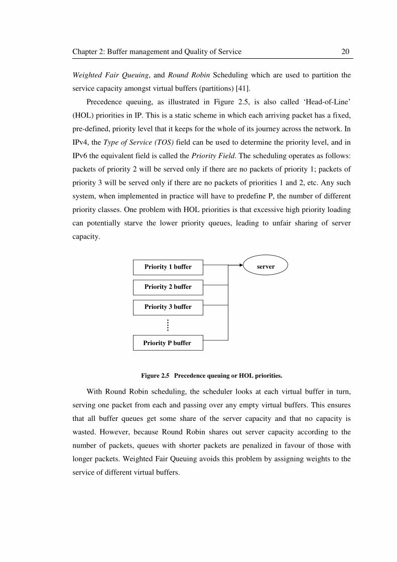
Chapter 2: Buffer management and Quality of Service 20
Weighted Fair Queuing, and Round Robin Scheduling which are used to partition the
service capacity amongst virtual buffers (partitions) [41].
Precedence queuing, as illustrated in Figure 2.5, is also called ‘Head-of-Line’
(HOL) priorities in IP. This is a static scheme in which each arriving packet has a fixed,
pre-defined, priority level that it keeps for the whole of its journey across the network. In
IPv4, the Type of Service (TOS) field can be used to determine the priority level, and in
IPv6 the equivalent field is called the Priority Field. The scheduling operates as follows:
packets of priority 2 will be served only if there are no packets of priority 1; packets of
priority 3 will be served only if there are no packets of priorities 1 and 2, etc. Any such
system, when implemented in practice will have to predefine P, the number of different
priority classes. One problem with HOL priorities is that excessive high priority loading
can potentially starve the lower priority queues, leading to unfair sharing of server
capacity.
Priority 1 buffer
Priority 2 buffer
Priority 3 buffer
Priority P buffer
server
Figure 2.5 Precedence queuing or HOL priorities.
With Round Robin scheduling, the scheduler looks at each virtual buffer in turn,
serving one packet from each and passing over any empty virtual buffers. This ensures
that all buffer queues get some share of the server capacity and that no capacity is
wasted. However, because Round Robin shares out server capacity according to the
number of packets, queues with shorter packets are penalized in favour of those with
longer packets. Weighted Fair Queuing avoids this problem by assigning weights to the
service of different virtual buffers.
Chapter 2: Buffer management and Quality of Service 21
2.2.3 Classification by granularity of priority assignment
For priority queuing schemes, priority assignment/handling can be either implicit or
explicit [30]. Priority can be specified at call level, at cell/packet level by the user or at
cell/packet level by the network [42]. Implicit policy assigns the same priority class to all
cells/packets of a service within a call. The choice of priority is done once and for all in
the network design and is kept fixed. For example in the case of Asynchronous Transfer
Mode (ATM) networks, the recognition of priority class of a given cell can be done
through the priority bit in the cell header itself or through the ATM virtual circuit
indicator (VCI) as specified at the set up of a call. In the case of (Internet Protocol) IP
networks, recognition of priority class can be done through the type of service (ToS)
field in IPv4 or the priority field in IPv6.
In the explicit policy alternative, the choice of the priority class of each cell/packet
of each call is performed by the source. This provides means to distinguish within a call
of a given service, the cells considered essential and requiring a better QoS with respect
to the others. This may be the case in video telephony, for instance, for the cells contain-
ing frame synchronization information whose loss can seriously degrade the service
quality. When explicit assignment policy is used, the recognition of the priority at the
network node level is obtained only via the information carried in the cell header. For
explicit loss priority assignment in ATM, the source marks the cells by setting the (cell
loss priority) CLP bit in the ATM cell header; while in an IP network the ToS field or
priority field is used to mark the packets.
2.3 Review of related work
2.3.1 Buffer Management in wireline networks
Some of the earlier work on buffer management such as [48] and [49] study strategies
for sharing a finite storage space between finite queues under the assumption of a single
traffic priority (i.e. without service class differentiation). Irland [48], investigates the
problem of sharing a finite number of packet buffers between several output queues in a
single packet switch, where buffer management policies restricting the sharing of
buffers are proposed and compared with unrestricted sharing policy (i.e. complete
sharing of total buffer space) and no sharing policy (i.e. complete partitioning of total

Chapter 2: Buffer management and Quality of Service 22
buffer space). In the paper, it is assumed that the switch has three output links of equal
transmission capacity and two kinds of traffic patterns were investigated. The first is a
balanced-load situation in which the variable traffic rate is split evenly between the three
output links, while the second is the unbalanced-load situation where the traffic rate for
only one link is varied while the other two links remained constant. His findings indi-
cated that while no sharing policy was simple to implement, it results in unnecessarily
large loss probability. Hence, throughput for no sharing policy is lowered compared to
the restricted sharing policies under balanced-load situation. Another crucial finding is
the behavior of the policies under the unbalanced-load situation. The unrestricted
sharing policy suffers sharp throughput degradation and remarkable increase in mean
delay, as the traffic increased beyond a point in the unbalanced-load situation unlike
with the other policies where the performance remained stable. This is indicative of a
major disadvantage of unrestricted buffer sharing i.e. the inability to effectively protect
other traffic from the saturation of one link. The study concluded that restricted sharing
of buffer space certainly improves the packet switch performance.
In [49], Kamoun and Kleinrock examine and analyze several schemes for sharing a
pool of buffers among a set of communication channels emanating from a given node in
a network environment so as to make effective use of storage in a variety of applications.
They consider a store-and-forward (S/F) computer network where the outgoing channels
of a node share a certain number of common buffers. The S/F function is modelled as a
set of M/M/1 queuing systems (one for each channel) sharing a common finite waiting
room. In the paper, they analyze the complete partitioning (CP) scheme (the simplest
scheme) where no sharing is provided, but the entire finite storage is permanently
partitioned among the servers (outgoing channels). The second scheme analyzed with
the model is the complete sharing (CS) scheme which accepts customers independent of
the server to which it is directed as long as there is available space.
Kamoun and Kleinrock found that complete sharing achieves a better performance
(i.e. lower probability of blocking) than complete partitioning under normal traffic
conditions and for fairly balanced input systems. However, they also found that for
highly asymmetrical message input rates and equal service rates, CS tends to favour
servers with the higher input rates even though they may be close to saturation (input
Chapter 2: Buffer management and Quality of Service 23
rate close to service rate). Furthermore, even with fairly balanced arrival rates under
overload conditions, CS fails (while CP succeeds) in securing a full utilization of the
servers. These observations suggests that contention for space must be limited in some
way; and in order to avoid the possible utilization of the entire space by any particular
output channel, they propose schemes that imposed a limit on the number of buffers to
be allocated at any time to any server namely: sharing with maximum queue lengths
(SMXQ), sharing with a minimum allocation (SMA) and sharing with a maximum queue
and minimum allocation (SMQMA). By comparing the blocking, delay and utilization
of the limited buffer sharing schemes with CS and CP they showed that in general,
sharing with some restriction on the contention for space is more advantageous than non-
sharing especially when little storage is available. While the approaches and proposed
buffer sharing schemes in [48] and [49] differ, their overall findings were essentially
similar.
Most of the works that followed tried to apply the same principles of buffer space
sharing to achieve loss priority management for different classes of services (with
different target cell loss probabilities) in ATM networks. In ATM, more emphasis was
laid on cell loss minimization due to absence of flow control and error recovery mechan-
isms. Without effective loss control mechanisms in ATM, higher layer protocols are
burdened with loss recovery/retransmissions thereby degrading performance and limit-
ing network resource utilization. Also, since transmission speed of a broadband (wired)
network is very high, the queuing delay and the delay jitter are small compared to the
propagation delay; hence, time priorities, usually termed as priorities were of limited
usefulness in the context of ATM [29], [50]. Because of these reasons, space priority
mechanisms for loss control to minimize end-to-end cell losses were studied much more
extensively compared to time priorities in ATM.
In [29], Kroner studies space priority mechanisms for buffer access in connection
with ATM networks. He describes different space priority mechanisms and compares
their performance. In the paper, a system with partial buffer sharing, another with
separate route (i.e. complete partitioning) for each traffic class, and a third system using
a push-out scheme and a common buffer as introduced in [51] and [52] are compared. In
the push-out scheme the selection of the cell to be discarded, as mentioned earlier, is
Chapter 2: Buffer management and Quality of Service 24
controlled by the replacement strategy which can be random, LIFO (last-in-first-out) or
FIFO (first-in-first-out). LIFO substantially minimizes the buffer management com-
plexity and is considered by Kroner in the studies, but using another replacement
strategy, e.g. random, results in slightly different loss probabilities according to results
presented in [52]. Kroner models the system as an M/G/1/N queuing system with two
classes of traffic with Poisson arrivals and exponential service times. The two traffic
classes represented two bearer services with different cell loss probability requirements
such that a medium quality transfer and high quality transfer where defined. In the
comparison of the different access schemes, the reported results confirmed the perfor-
mance gains that accrue from the use of priorities in ATM networks for various load
situations. The partial buffer sharing system was seen to perform reasonably well
compared to the push-out system, but partial buffer sharing with adaptive threshold was
shown to give better performance than with fixed threshold in the same evaluation.
However, the paper did not detail the specific algorithm to implement partial buffer
sharing with adaptive threshold.
In [34], Kroner, Hebuterne and Boyer also extended the work in [29] to evaluate the
performance of the buffer access schemes for bursty input traffic. The main conclusion
drawn from their studies is that while the push-out mechanism achieved the highest load
improvement, the relatively simpler partial buffer sharing mechanism provides for very
close performances and should be preferred for its ease of implementation. Furthermore,
they argue that the basic advantage of selective discarding mechanisms (i.e. partial
buffer sharing and push-out) is that it makes the network able to cope with bursty traffic,
a property which cannot be achieved by any practical over dimensioning.
In [50], Rothermel observes that loss priority mechanisms implies an increase in the
maximum admissible load in ATM pipes or a decrease of the necessary size of buffers in
ATM switches. Thus, in his work he attempts to determine the increase in admissible
load gained by the use of priorities at given buffer sizes, and, also the reduction in buffer
size caused by the use of priorities at a given admissible load. The priority mechanisms
assumed is the ‘threshold scheme’ i.e. partial buffer sharing in which a threshold T
provides the upper limit for accepting low priority packets into the shared buffer of a
fixed size S. The model used assumes Poisson arrivals from two classes with uniform
Chapter 2: Buffer management and Quality of Service 25
distribution of class 1 and class 2 cells over N outlets. His findings suggest that the use
of priorities increase the admissible load slightly in the case of Poisson arrivals. Howev-
er, buffer space savings of 15-20 % were obtainable even with highly unbalanced traffic
mix (i.e. larger portion of high priority traffic). The results also affirm that a fixed
threshold cannot be optimal all the time as total load and load ratio are prone to fluctua-
tion in practice, therefore necessitating ‘adaptive’ threshold for optimum performance.
In [28], Kang and Tan present a theoretical analysis of the cell loss probability per-
formance of an explicit priority assignment partial buffer sharing scheme for ATM
networks. Their work too was motivated by the incorporation of two bearer services with
different levels of cell loss probability QoS requirements in ATM networks, with low
priority service having a weaker cell loss probability constraint than the higher priority
service. They propose explicit priority assignment in which each individual cell is
marked at the source as being either essential or ordinary, with the essential cells being
of higher priority with more stringent cell loss probability constraint. They considered a
two service class traffic model in which each traffic class consists of bursty traffic
generated by a multiple number of Markov sources. Each Markov source is modelled by
a three-state Discrete-Time-Markov-Chain (DTMC) with a high priority state, low
priority state and an idle (off) state. Kang and Tan noted in their work that besides the
added advantage of flexibility, the explicit priority assignment yielded similar advantag-
es for partial buffer sharing control compared to the implicit policies analyzed in [33] by
Bae, Suda and Simha, and in [53] by Hou and Wong.
In [25], Causey and Kim present a comparison of buffer allocation schemes in ATM
switches where they compare complete sharing, partial sharing and dedicated allocation
by simulation. They argue that although complete buffer sharing is superior to dedicated
allocation under non-bursty traffic due to the statistical gains that derive from sharing
buffers, this generalization is not valid for some bursty traffic patterns. The reason given
for this is because completely shared buffers may be plagued by congestion arising from
a few bursty calls unfairly occupying the entire buffer space to the exclusion of other
calls. Thus under bursty traffic conditions two competing forces exist in a completely
shared system: gains due to sharing and losses due to unfairness. Dedicated queues are
intrinsically fair but do not enjoy the statistical gains of sharing. The magnitude of these
Chapter 2: Buffer management and Quality of Service 26
two competing factors (sharing and fairness) varies with the average burst length of the
incoming traffic. Thus, shared queues may be the best in one traffic environment, while
dedicated queues may perform better in another environment. Hence, Causey and Kim
state that partial buffer sharing offers a compromise between complete sharing and
dedicated allocation by obtaining some gains from sharing while maintaining a degree of
fairness.
In [40], Lin and Silvester also evaluate priority bandwidth and buffer management
in ATM communication nodes. They consider different loss priority queuing strategies,
differing in the degrees of resource sharing, namely complete sharing with pushout and
head-of-the-line (CS+PO+HOL), partial buffer sharing, complete buffer partitioning but
complete bandwidth sharing (CBP+CBWS) , and complete partitioning (CP). They
consider a discrete-time multichannel queuing system with finite buffer capacity,
D{A1,A2}/D/c/B queue for performance evaluation of the schemes. The CS+PO+HOL
scheme is a modification of the CS+PO scheme in which the service discipline is the
head-of-the-line where class 1 cells join the queue as well as transmission registers
ahead of all class 2 cells and cells within the same priority class are transmitted on a
FCFS basis. Note that with HOL service discipline, the CS+PO+HOL scheme attaches
both space and time priorities to the high priority (class 1) cells, unlike in the CS+PO
scheme with FCFS discipline which gives only space priority (to class 1 cells). In the
CBP+CBWS scheme, since the bandwidth is shared, the buffer partition for a given total
buffer size B is adjusted to satisfy various loss QoS requirements; i.e. the so-called
adaptive CBP.
Lin and Silvester also refer to CS+PO+HOL scheme as absolute priority queuing,
because it provides the most preferential treatment in term of both loss probability as
well as delay to the higher-priority traffic class. They point out that this characteristic
may not be desirable because many loss-sensitive services such as distributed computing
impose almost little or no delay requirements, whereas many time-constrained services
such as voice or interactive video can tolerate a relatively higher loss rate (on the order
of 10-2
). Another potential problem is that the implementation complexity could be
prohibitive. Nevertheless, their results suggest that (space) priority systems can provide
substantial improvement to high priority class at little cost to the low priority class.
Chapter 2: Buffer management and Quality of Service 27
Another paper that considers space priority management in shared memory ATM
switch is the one by Choudhury and Hahne [42]. They present a simulation study of
several ways to manage space priorities in a shared memory ATM switch in which the
queues for the switch output ports share space flexibly in a common buffer. Their
findings support a “Selective Pushout” strategy over the other schemes. In their work
they focus on providing different loss QoS to different classes of variable bit rate (VBR)
traffic. Thus the high priority traffic and low priority traffic considered are both very
bursty. Similar to the aforementioned works, delay priority is disregarded since constant
bit rate traffic (CBR) which typically requires delay priority is not incorporated in their
study. The buffer management schemes analyzed include threshold mechanisms, pu-
shout mechanisms and various hybrids of threshold and pushout mechanisms.
The first threshold-based option imposed a Global Threshold on the total number of
cells in the shared memory. The alternative option places Individual Thresholds on the
queue length associated with each output queue. For the pushout mechanism, two kinds
are considered: Selective Pushout and Non-Selective Pushout. In Selective Pushout, a
high priority cell that arrives to find the buffer full is allowed to enter by pushing out a
low priority cell, but does not take over its position in its logical FIFO queue. Instead,
the high priority cell joins the tail of the logical FIFO queue for its own output. In
addition, the high priority cell pushes out from the longest output queue containing any
low priority cells. This allows smaller queues to increase in length at the expense of
longer queues thereby creating a degree of fairness in the sharing of buffer space
amongst the output queues. It also tends to keep more memory outputs busy which
increases the efficiency of the system.
Selective Pushout incurs high implementation overhead because it requires keeping
track of the priority of each cell in the shared memory. The system must also maintain
enough pointers to be able to mend an output’s logical FIFO queue whenever a low
priority cell is pushed out from the middle of that FIFO. With Non-Selective Pushout, an
arriving high priority cell that finds the buffer full pushes out the cell at the head of the
longest queue regardless of priority. This means that a high priority cell may be pushing
out another high priority cell even when there are low priority cells present in the buffer.
A low priority cell that arrives to a full buffer is simply blocked. While not as sophisti-
Chapter 2: Buffer management and Quality of Service 28
cated as Selective Pushout, Non-Selective Pushout still offers some advantage to high
priority traffic, equalizes the output queues, and only needs to keep track of output queue
lengths.
Hybrid schemes combine Selective or Non-Selective Pushout with Global or Indi-
vidual Thresholds. Choudhury and Hahne found that Selective Pushout was a more
effective mechanism for space priorities than Non-Selective Pushout. For threshold
schemes they conclude that Global Thresholds were more effective for space priories
than Individual thresholds. Also, systems with only pushout schemes were seen to have
lower overall total loss than systems with no priority mechanisms at all; these systems in
turn had lower total cell loss than systems with only thresholds. The pure pushout
schemes were more efficient than the hybrids, which were in turn more efficient than the
pure threshold schemes as far as overall cell loss was concerned. For various load
patterns studied, Selective Pushout showed better overall performance with low overall
cell loss rate and very low losses for high priority cells.
In [54], A proposal by Chao and Uzan that attempts to provide both delay and loss
priorities in ATM can be found. It utilizes a pushout policy with multiple delay and loss
priorities. During a call set up each service is assigned to a service class determined by a
delay and a loss priority. A queue manager in the ATM network nodes then schedules
the cell discarding and departing sequence based on their delay and loss priorities. The
buffer is completely shared by all service classes and a pushout discarding mechanisms
is used. In their proposal assignment of delay and loss priorities can be completely
independent, unlike with the CS+PO+HOL scheme proposed in [42] which assigns the
so-called absolute priority to the high priority services to receive the most preferential
treatment of both delay and loss rates. The queue manager at each output port of an
ATM output buffered switch is responsible for scheduling higher-delay-priority cells to
be transmitted sooner, and higher-loss-priority cells to be discarded last when the buffer
is full. Pushout scheme is adopted because it does not require threshold setting thereby
eliminating the need to know any traffic information.
Their proposed scheme utilizes a priority matrix as shown in Table 2.1, with four
different service classes, I, II, III, and IV. The cell departing sequence among the classes
is assumed to be I → II → III → IV (class I preceding class II, class II preceding class
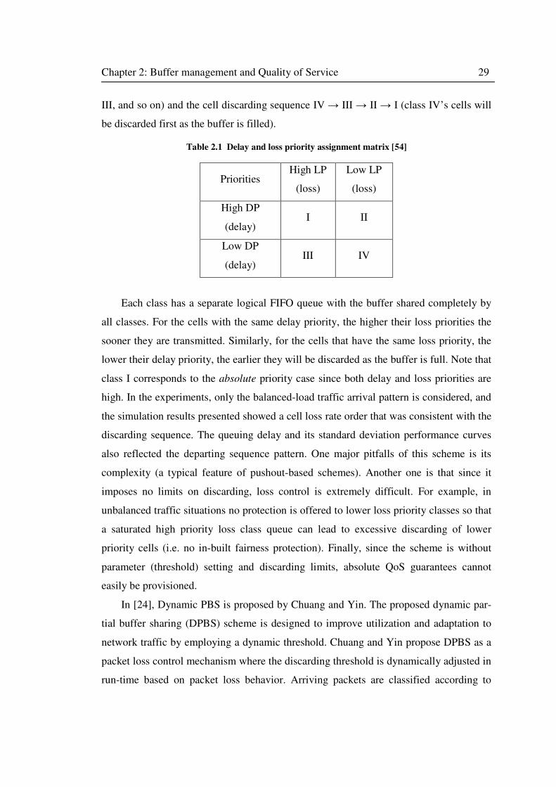
Chapter 2: Buffer management and Quality of Service 29
III, and so on) and the cell discarding sequence IV → III → II → I (class IV’s cells will
be discarded first as the buffer is filled).
Table 2.1 Delay and loss priority assignment matrix [54]
Priorities High LP
(loss)
Low LP
(loss)
High DP
(delay) I II
Low DP
(delay) III IV
Each class has a separate logical FIFO queue with the buffer shared completely by
all classes. For the cells with the same delay priority, the higher their loss priorities the
sooner they are transmitted. Similarly, for the cells that have the same loss priority, the
lower their delay priority, the earlier they will be discarded as the buffer is full. Note that
class I corresponds to the absolute priority case since both delay and loss priorities are
high. In the experiments, only the balanced-load traffic arrival pattern is considered, and
the simulation results presented showed a cell loss rate order that was consistent with the
discarding sequence. The queuing delay and its standard deviation performance curves
also reflected the departing sequence pattern. One major pitfalls of this scheme is its
complexity (a typical feature of pushout-based schemes). Another one is that since it
imposes no limits on discarding, loss control is extremely difficult. For example, in
unbalanced traffic situations no protection is offered to lower loss priority classes so that
a saturated high priority loss class queue can lead to excessive discarding of lower
priority cells (i.e. no in-built fairness protection). Finally, since the scheme is without
parameter (threshold) setting and discarding limits, absolute QoS guarantees cannot
easily be provisioned.
In [24], Dynamic PBS is proposed by Chuang and Yin. The proposed dynamic par-
tial buffer sharing (DPBS) scheme is designed to improve utilization and adaptation to
network traffic by employing a dynamic threshold. Chuang and Yin propose DPBS as a
packet loss control mechanism where the discarding threshold is dynamically adjusted in
run-time based on packet loss behavior. Arriving packets are classified according to
Chapter 2: Buffer management and Quality of Service 30
multiple discarding priorities, and multiple discarding thresholds are deployed during
run time. Being a PBS scheme, arriving packets are admitted into the queue of the DPBS
only if its current occupancy is less than its discarding threshold; otherwise only high
priority packets are admitted until the queue is full. A packet loss counter is used for
each discarding priority to record the number of discarded packets and each increment of
the loss counter for high priority packets pushes the discarding threshold to decrease,
whereas each increment of the loss counter for low priority packets pushes the discard-
ing threshold to increase. In the experiments, both exponential traffic and Pareto traffic
are considered. Simulation results are presented showing that DPBS outperforms Static
Partial Buffer Sharing (SPBS) schemes such as the one in [28] under the same traffic
conditions, thus achieving higher buffer utilization due to its adaptation to network
conditions.
In a recent paper [55], Kausha and Sharma present the analysis of an Adaptive Par-
tial Buffer Sharing Scheme (APBS) similar to the DPBS scheme proposed by Chuang
and Yin but with emphasis on consecutive packet loss reduction. APBS performance is
compared with complete buffer sharing (FIFO) and SPBS schemes. Their algorithm is
designed to dynamically vary the PBS threshold in run-time based on the packet loss
behavior of the priority classes in order to reduce consecutive packet losses. The main
observation from their work is that an adaptive threshold (in APBS scheme) performs
better for the kind of traffic that has a higher proportion in the input traffic mix. For
example, when the input traffic mix has major content of high priority packets, the
consecutive packet loss of high priority packets significantly decreases as compared to
low priority packets and vice-versa. This characteristic of ADPBS illustrates its efficient
control and adaptive nature. Overall, ADPBS manages to reduce consecutive packet loss
as compared to SPBS and FIFO queues due to its adaptive threshold nature.
In [56], Awan and Al-Begain, investigate an enhanced PBS scheme where two
classes of flows, one of which is delay sensitive (high priority) and the other, loss
sensitive (low priority), arrive at the finite buffer. In their proposed PBS scheme, the
high priority (delay sensitive) packets are only allowed access to the buffer when the
total number of packets is below the pre-determined threshold; otherwise, only the low
priority (loss sensitive) packets can access the buffer until it becomes full. The scheme
Chapter 2: Buffer management and Quality of Service 31
only differs from classical PBS schemes in the sense that the low loss priority is attached
to the delay sensitive flow, but no (logical) precedence queuing is employed as the
packet ordering is in FCFS basis regardless of priority. Hence, it lacks time/transmission
or service prioritization, which will not only compromise the jitter performance of the
delay sensitive class, but also limit the achievable delay performance since the loss
sensitive packets have access to transmission even when delay sensitive packets are
present in the buffer.
2.3.2 Buffer management in wireless networks
As a means to provide effective sharing of bottleneck resources for enhanced QoS
support, some researchers have studied buffer management in wireless environments. In
a recent paper by Orlov and Necker [57], an investigation of how buffer management
strategies within the Radio Access Network (RAN) of a HSDPA network can alleviate
the impact of an unreliable and time-varying link on the quality of non-interactive video
streaming services is presented. They discuss the pros and cons of proactive and reactive
approaches, whilst proposing proactive buffer management schemes with data differen-
tiation to improve the MPEG-4 video quality.
In reactive approach, the scheme becomes active when a congestion situation has
already occurred i.e. when the buffer queue is full. In the paper, buffer management
without data differentiation is considered the reactive approach. The first reactive
approach discussed is the frame-based drop-tail FIFO buffer management which drops
all IP packets belonging to the same video frame if one of its IP packets was lost or
dropped. Note that this approach is basically the Complete Buffer Sharing (CBS) scheme
described earlier but with a frame-based drop-tail discard. The other reactive approach is
the drop-head (frame discard) strategy where those data units that reside the longest in
the queue are dropped. With this approach, the transmission of video data that may
arrive too late at the client is suppressed in favour of newly arriving data. Note that this
drop-head strategy is equivalent to the Pushout with FIFD replacement strategy de-
scribed and illustrated earlier in section 2.2.1
The buffer management with data differentiation discussed by Orlov and Necker in
the paper are variations of the Partial Buffer Sharing (PBS) mechanism, which also
Chapter 2: Buffer management and Quality of Service 32
makes them space priority buffer management schemes. In their schemes, prioritization
is based on the ‘importance’ of the arriving video frame. In an MPEG encoded frame,
the loss of a ‘B-frame’ has less impact on quality than the loss of an ‘I- or P-frame’; thus
from the buffer management viewpoint, the latter has lower loss priority while the
former have higher loss priority. Thus in the proactive approach, the buffer will proac-
tively drop packets containing data of B-frames if the buffer occupancy exceeds a given
threshold δ (i.e. a typical PBS scheme). This can be done either on a packet basis or a
frame basis, thus resulting in two different proposed proactive approaches namely:
Packet-based proactive B-dropping and Frame-based proactive B-dropping. In a
nutshell, Orlov and Necker’s work demonstrated that the objective video quality of a
streamed non-interactive video-on-demand-content in a wireless environment can
significantly be improved by means of application-aware buffer management, which
takes into account video frame priorities and video frame dependencies. In related
works, a simple video frame discard scheduling algorithm with data differentiation in a
Wireless LAN environment is presented in [58], while the proactive mechanism FDDT
(Frame-Level Packet Discard With Dynamic Thresholds) is proposed and evaluated in a
fixed-network one-link scenario in [59].
Another related work [60] considers several space priority schemes under various
acronyms, for the Radio Link Control (RLC) layer buffer management for video stream-
ing over a HSDPA shared channel. The schemes are referred to as: Drop New Arrivals
(DNA) which is equivalent to drop-tail CBS; Drop Random Packet (DRP), which is
equivalent to Pushout with Random replacement strategy discussed in section 2.2.1;
Drop HOL Packet (DHP), which is basically the same as Pushout with FIFD replace-
ment. Liebl et. al. concluded in the study, that for the video streaming application, the
optimal dropping strategy for incoming IP packets at the radio link buffer is to drop the
packet with the longest waiting time in the buffer (i.e. DHP policy), since it is most
likely packet to have an expired arrival deadline.
In [61], Awan and Al-Begain propose and evaluate a buffer management scheme for
3G UMTS networks. The scheme is based on multi-level priority and Complete Buffer
Sharing (CBS) policy for all buffers at the border and inside the wireless network. They
employ an analytical model based on the G/G/1/N queue with single server and R (R ≥
Chapter 2: Buffer management and Quality of Service 33
2) priority classes under the Head of Line (HOL) service rule for the CBS scheme. Their
findings showed that the buffer management scheme provided higher QoS for the higher
priority classes.
Other works in the literature related to application of buffer management for QoS
enhancement in wireless networks can be found in [62-65]. Thus, there is growing
interest in employing buffer management-based solutions to enhance traffic QoS per-
formance in wireless networks. However, the issue of QoS management of multimedia
sessions with multiplexed services comprising concurrent diverse flows in a single user
session is not fully addressed by the existing buffer management schemes proposed for
wireless environments in the literature.
2.4 Service differentiation for QoS support in mobile networks
Since the main focus of this thesis is on buffer management based QoS control of
multimedia services in UMTS High Speed Downlink Packet Access, discussions here
are limited to the UMTS mobile systems. In order to facilitate QoS management in
incumbent mobile networks expected to support a wide range of applications that have
different QoS characteristics, service class differentiation is an essential requirement.
According to [66], an application is defined as a task that requires communication of one
or more information streams, between two or more parties that are geographically
separated, while a set of applications with similar characteristics can be classified as a
service. QoS mechanisms utilize service classes to provision different levels of service
quality. In mobile networks, a possible way to maintain end-to-end QoS is to over-
dimension/over-provision the radio link resources since this is where the main bottleneck
to end-to-end communication exists. However, this is a very inefficient approach be-
cause of the variable and unpredictable nature of the radio link. Moreover, the technical
requirements for UMTS QoS specified by 3GPP states amongst other things, that [67]:
“QoS shall support efficient resource utilization”. In order to allow different levels of
QoS provisioning, 3GPP defines four distinct service classes for the UMTS system
which are described below.
Chapter 2: Buffer management and Quality of Service 34
2.4.1 UMTS QoS classes
According to [67], the QoS mechanisms provided in the cellular network have to be
robust and capable of providing reasonable QoS resolution. Table 2.2 illustrates the QoS
classes for UMTS. There are four different QoS classes:
- conversational class;
- streaming class;
- interactive class; and
- background class.
Conversational class is meant for traffic that is very delay sensitive while Back-
ground class is the most delay insensitive traffic class. Conversational and Streaming
classes are mainly intended to be used to carry real-time traffic flows. The main distin-
guishing factor between them is the delay sensitivity of the traffic. Conversational real-
time services, like video telephony, are the most delay sensitive applications and their
data streams should be carried in the Conversational class. Conversational class applica-
tions are transmitted as real-time connections, with communications always performed
between live end-users. Furthermore, this is the only type where the required characteris-
tics are strictly imposed by human perception. The end-to-end delay requirement is low
(typically 200ms or less) and the traffic is nearly symmetric. Speech service, VoIP,
video telephony are some examples of conversational class applications.
Streaming is a technique for transferring data such that it can be processed as a
steady continuous stream (e.g. viewing and listening to media in real-time). The client
browser can start displaying the data before the entire file has been transmitted. Thus,
the term ‘streaming’ refers to an application playing unidirectional, synchronized (if
several media streams are involved) and continuous media stream(s), while those
streams are being transmitted over the data network [68]. Streaming applications can
also be further divided into ‘on-demand’ and ‘live’ information delivery. Examples of
the first type are music and news-on-demand applications; the latter category can include
live delivery of radio and television programmes.
Interactive class is applied when the end-user (human or machine) is requesting da-
ta from the remote equipment. It is characterized by the request-response pattern of the
end-user and the contents of the packets must be transparently transferred (i.e. low bit
Chapter 2: Buffer management and Quality of Service 35
error rate). Hence, one of the key properties of this class is the service response time.
The service response time can be defined as the period elapsed between the time of the
data request and the end of the message reception, which determines the degree of
satisfaction perceived by the end user. Web browsing, server access and database
retrieval, location-based services and computer games are examples of human interac-
tion, while automatic database enquiries (tele-machines) and polling for measurement
records are examples of machine interaction with remote equipment.
Background class comprise of applications that are more or less insensitive to deli-
very time. This is because the destination is not expecting the data within a certain time,
so the delay can range from seconds up to minutes. Interactive and Background classes
are mainly meant to carry non-real time (NRT) traffic e.g. traditional Internet applica-
tions like WWW, Email, Telnet, FTP and News. Due to less stringent delay
requirements, compared to conversational and streaming classes, both Interactive and
Background provide better error rate by means of channel coding and retransmission.
The main difference between Interactive and Background class is that Interactive class is
mainly used by interactive applications, e.g. interactive Web browsing, while Back-
ground class is meant for background traffic, e.g. background download of Emails or
background file downloading, SMS, reception of measurement records etc, which do not
require immediate action. Responsiveness of the interactive applications is ensured by
separating interactive and background applications. Traffic in the Interactive class has
higher priority in scheduling than Background class traffic, so background applications
use transmission resources only when interactive applications do not need them. This is
very important in wireless environment where the bandwidth is low compared to fixed
networks.
These are only typical examples of usage of the traffic classes. There is no particular
strict one-to-one mapping between classes of service and the traffic classes. For instance,
a service interactive by nature can very well use the Conversational traffic class if the
application or the user has tight requirements on delay.
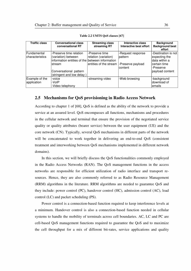
Chapter 2: Buffer management and Quality of Service 36
Table 2.2 UMTS QoS classes [67]
Traffic class Conversational class conversational RT
Streaming class streaming RT
Interactive class Interactive best effort
Background Background best
effort
Fundamental characteristics
-Preserve time relation (variation) between information entities of the stream Conversational pattern (stringent and low delay )
-Preserve time relation (variation) between information entities of the stream
-Request response pattern -Preserve payload content
-Destination is not expecting the data within a certain time -Preserve payload content
Example of the application
-voice -VoIP -Video telephony
-streaming video -Web browsing -background download of emails
2.5 Mechanisms for QoS provisioning in Radio Access Network
According to chapter 1 of [68], QoS is defined as the ability of the network to provide a
service at an assured level. QoS encompasses all functions, mechanisms and procedures
in the cellular network and terminal that ensure the provision of the negotiated service
quality or quality attributes (bearer service) between the user equipment (UE) and the
core network (CN). Typically, several QoS mechanisms in different parts of the network
will be concatenated to work together in delivering an end-to-end QoS (consistent
treatment and interworking between QoS mechanisms implemented in different network
domains).
In this section, we will briefly discuss the QoS functionalities commonly employed
in the Radio Access Networks (RAN). The QoS management functions in the access
networks are responsible for efficient utilization of radio interface and transport re-
sources. Hence, they are also commonly referred to as Radio Resource Management
(RRM) algorithms in the literature. RRM algorithms are needed to guarantee QoS and
they include: power control (PC), handover control (HC), admission control (AC), load
control (LC) and packet scheduling (PS).
Power control is a connection-based function required to keep interference levels at
a minimum. Handover control is also a connection-based function needed in cellular
systems to handle the mobility of terminals across cell boundaries. AC, LC and PC are
cell-based QoS management functions required to guarantee the QoS and to maximize
the cell throughput for a mix of different bit-rates, service applications and quality
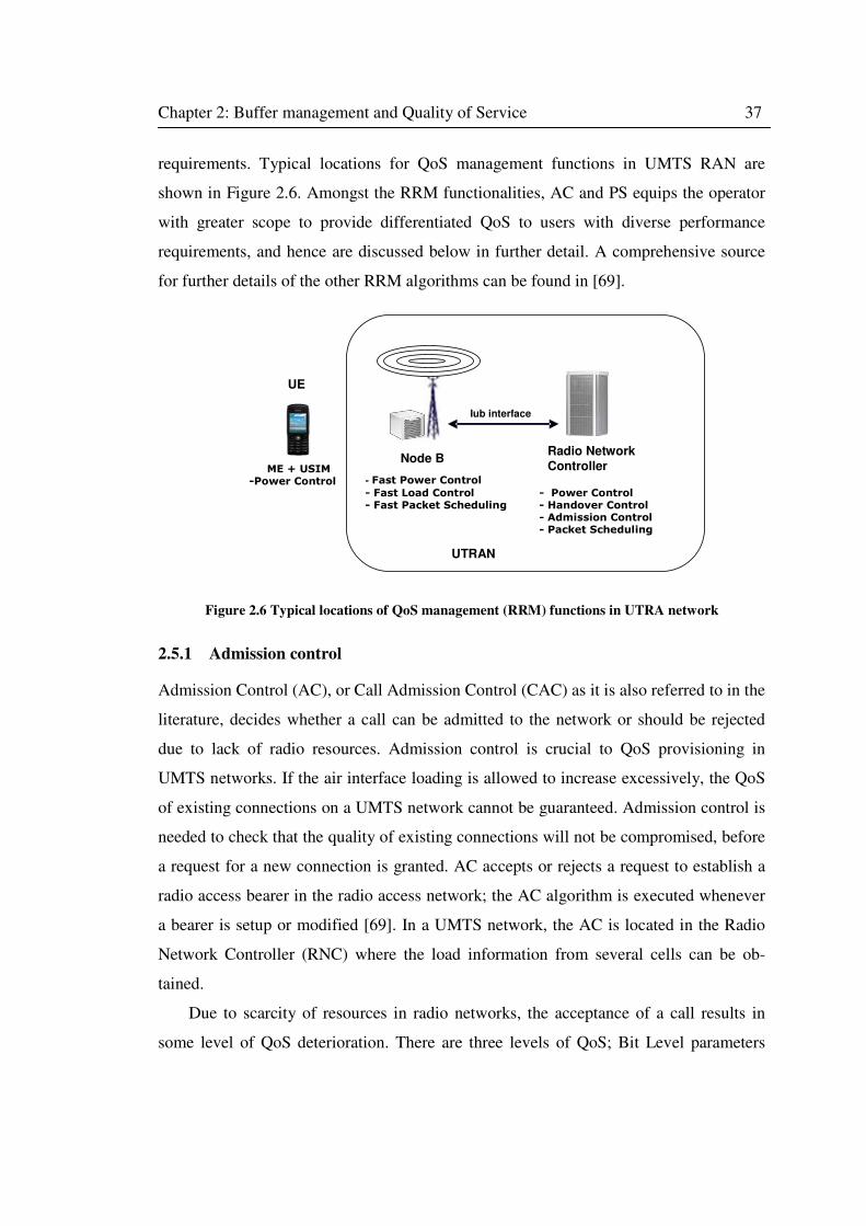
Chapter 2: Buffer management and Quality of Service 37
requirements. Typical locations for QoS management functions in UMTS RAN are
shown in Figure 2.6. Amongst the RRM functionalities, AC and PS equips the operator
with greater scope to provide differentiated QoS to users with diverse performance
requirements, and hence are discussed below in further detail. A comprehensive source
for further details of the other RRM algorithms can be found in [69].
ME + USIM-Power Control
Radio Network Controller
Iub interface
Node B
UE
- Fast Power Control
- Fast Load Control- Fast Packet Scheduling
- Power Control- Handover Control- Admission Control- Packet Scheduling
UTRAN
Figure 2.6 Typical locations of QoS management (RRM) functions in UTRA network
2.5.1 Admission control
Admission Control (AC), or Call Admission Control (CAC) as it is also referred to in the
literature, decides whether a call can be admitted to the network or should be rejected
due to lack of radio resources. Admission control is crucial to QoS provisioning in
UMTS networks. If the air interface loading is allowed to increase excessively, the QoS
of existing connections on a UMTS network cannot be guaranteed. Admission control is
needed to check that the quality of existing connections will not be compromised, before
a request for a new connection is granted. AC accepts or rejects a request to establish a
radio access bearer in the radio access network; the AC algorithm is executed whenever
a bearer is setup or modified [69]. In a UMTS network, the AC is located in the Radio
Network Controller (RNC) where the load information from several cells can be ob-
tained.
Due to scarcity of resources in radio networks, the acceptance of a call results in
some level of QoS deterioration. There are three levels of QoS; Bit Level parameters
Chapter 2: Buffer management and Quality of Service 38
such as energy-to-noise ratio [70]. The second level is Packet Level parameters such as
packet loss, while the third level is the Call Level with blocking and dropping probabili-
ties as the main QoS parameters. The decision to accept or reject a call is dependent
upon the capacity measurement descriptors, which differ for the different level of QoS,
as discussed above. For instance, interference, bit rate, and number of calls in a connec-
tion. The major goals of AC schemes are to [71]:
• maximize channel utilization in a fair manner to all flows,
• minimize the dropping probability of handover calls,
• minimize the reduction of service of connected calls,
• minimize the blocking probability of new calls.
In UMTS networks with High Speed Downlink Packet Access (HSDPA), the ad-
mission control decision is taken by the RNC (see Figure 2.6). For packet-switched
services, the AC algorithm in the RNC needs to consider the QoS parameters provided
by the core network as well as the general resource situation in the network. If only best
effort traffic (interactive and background) with no strict QoS requirements are transmit-
ted on HSDPA , then the AC algorithm can be made fairly simple by only checking the
availability of radio access network (RAN) resources to serve a new HSDPA user (or
handover an existing one from one cell to another). If more services with stricter QoS
requirements such as conversational or streaming class services are considered for
HSDPA, then a more advanced admission control algorithm is needed to ensure that the
QoS requirements of existing HSDPA users in the cell as well as those of the new user
can be fulfilled after potential admission. Examples of quality-based HSDPA access
control algorithms are studied in [72] and [73], where QoS attributes of new HSDPA
users are taken into account in admission control decisions. Hence, using this type of
algorithm, high-priority users tend to experience a lower blocking probability than low-
priority users.
2.5.2 Packet scheduling
While AC algorithms admit calls based on availability of resources and QoS require-
ments at call level, Packet Scheduling algorithms are responsible for packet-level
allocation of shared resources to already admitted users/flows. The major goal of the
Chapter 2: Buffer management and Quality of Service 39
Packet can be stated as maximizing the network throughput (capacity) while satisfying
the QoS of the admitted users. In the earlier Release 99 UMTS, the RNC was responsi-
ble for packet scheduling while the Node B merely transmitted the packets over the air
interface. With Release 5 (i.e. HSDPA) however, the UMTS architecture is modified by
moving the packet scheduler from the centralized RNC to the Node B where it is em-
bedded in a new medium access control (MAC) entity called the MAC high speed
(MAC-hs) [74]. This was illustrated in Figure 2.6 as Node B fast packet scheduling.
Packet scheduling plays a crucial role in HSDPA. With the purpose of enhancing
the cell throughput (capacity), the HSDPA scheduling algorithm can take advantage of
the instantaneous channel variations and temporarily raise the priority of the favourable
users. Since the users’ channel quality vary asynchronously, the time-shared nature of
HS-DSCH introduces a form of selection diversity with important benefits for the
spectral efficiency [75]. However, this could mean those users more distant from the
Node B (at cell edge) and therefore requesting lower data rates could be starved for
service. Consequently, the scheduling algorithms must balance the conflicting goals of
maximizing the throughput, while at the same time ensuring some degree of fairness to
all users requesting a service [76].
Several packet scheduling algorithms have been proposed for HSDPA in the open
literature. Gutierrez [75] classifies the well known HSDPA packet scheduling algorithms
into two groups according to the pace of the scheduling process:
• Fast Scheduling methods: i.e. PS methods that base the scheduling decision
on the recent UE channel quality measurements (i.e. executed on a TTI ba-
sis) to allow tracking of the instantaneous variations of the user’s supported
data rate. These include Maximum C/I, Proportional fair, and Fast Fair
Throughput.
• Slow Scheduling methods: These are PS methods that base their scheduling
decisions on the average user’s signal quality such as Average C/I, or those
that do not use any user’s performance metrics at all such as Round Robin.
Note that the aforementioned basic scheduling algorithms do not take into account
queuing or the amount of user buffered data, nor are they designed to take packet delay
requirements into consideration. It is also pertinent to note that these algorithms offer
Chapter 2: Buffer management and Quality of Service 40
scheduling on a per user basis (under the assumption of a single flow per user), as such,
they would not adequately support the QoS of users with multiple flows or multip-
lexed/multimedia services.
In order to support delay differentiation, some researchers propose modifications of
the existing basic PS algorithms to include queuing delay. For example, the Modified
Largest Weighted Delay First (M-LWDF) algorithm [77], which not only takes advan-
tage of the multiuser diversity available in the shared channel available through the
Proportional Fair algorithm, but also increases the priority of flows with head of line
packets close to their deadline violation. Other similar modifications/extensions of the
proportional fair algorithm to support delay differentiation include the Earliest Due
Deadline (EDD) [78], and the Exponential Rule (ER) [79].
These algorithms while being able to provide delay differentiation also have metrics
for per user scheduling decisions only; the scheduling metrics do not include provisions
for class differentiation between flows belonging to the same user. In order to address
this problem, Golaup et. al modify the M-LWDF algorithm to allow for inter-class
prioritization in addition to inter-user prioritization thus supporting class differentiation
between flows of the same user. They term their algorithm, the Largest Average
Weighted Delay First (L-AWDF) [80]. The basic idea behind L-AWDF is that it main-
tains a Proportional Fair (PF) factor for fairness in respect of channel conditions, while
giving transmission priority to those users whose scheduled packets are nearing the
maximum allowable delays for their class through a relative delay factor; this is con-
structed in such a way as to allow traffic class performances to be influenced by different
weighting factors. Note that in this algorithm, the priority of each class of traffic/flow is
expressed through the specification of a maximum allowable delay and a selected
weighting factor.
While this type of packet scheduling approach does provide class differentiation to
support users that are running several applications simultaneously, it does not take buffer
or queue management into account. Whereas, because the packet scheduling functionali-
ty necessitates data buffering at the edge of the radio access network, where the
bottleneck to end-to-end communication exists, buffer management techniques are vital
to enhancing network and radio resource utilization as well as improving traffic perfor-
Chapter 2: Buffer management and Quality of Service 41
mance. Most importantly, buffer management will allow for QoS control to cater for the
diverse performance requirements of multiple flows simultaneously transmitted to the
same user on HSDPA shared channel.
2.5.3 Benefits of RAN buffer management
The benefits of employing buffer management schemes at the bottleneck edge node
(base station), rather than relying on packet scheduling algorithms and admission control
alone for QoS provisioning, are manifold. Some of the major benefits include:
• Queue-based service differentiation: Most of the existing HSDPA packet
scheduling algorithms are designed for inter-user/multi-user scheduling un-
der assumption of single flow or class per user. Buffer management schemes
can be designed to allow such algorithms cope with multiple classes of traf-
fic per user, by enabling differentiated queuing mechanisms. For example, a
buffer management scheme could be used for priority handling of the head-
of-line packets of different classes of flows (with separate queues) for the
same user, to co-ordinate prioritized packet transmissions during the user’s
transmission opportunity scheduled by the inter-user/multi-user scheduling
algorithm.
• Enhanced QoS control: Buffer management schemes can allow not only
(relative) delay differentiation, but also loss differentiation through effective
buffer access control mechanisms. This multi-dimensional differentia-
tion/prioritization property of buffer management allows various
combinations of different types of priorities to be attached to multiple flows
thereby enabling a more powerful QoS control capability. This is a feature
which even (inter-user/multi-user) packet scheduling algorithms that allow
inter-class prioritization between flows of the same user cannot very easily
provide.
• Efficient buffer utilization: The efficient utilization of buffer space can
lead to improved traffic performance. Buffer management schemes in the
bottleneck node could be designed to discard or pushout ‘useless’ packets
Chapter 2: Buffer management and Quality of Service 42
(depending on the scheme) to create more room; or employ any other tech-
nique that ensures the efficient utilization of the buffer capacity.
• Flexibility: Buffer management allows inter-class priority handling to be
separated from the inter-user packet scheduling functionality; thus allowing
efficient buffer management schemes to be designed for priority handling
and QoS control while re-using existing packet scheduling (and admission
control schemes). This scheduler-independent approach to buffer manage-
ment at the cellular network bottleneck (radio link) allows for greater
flexibility in deploying different combination of solutions.
2.6 Chapter summary
Buffer management has been discussed in this chapter as a fundamental QoS control
mechanism that uses certain policies to assign buffer resources amongst different flows
or aggregation of flows. Buffer management schemes can be classified into complete
partitioning policy based (CPB), partial buffer sharing (PBS) policy based or complete
buffer sharing (CBS) policy based, from resource management viewpoint. When consi-
dered from service differentiation perspective, most buffer management schemes fall
under either time or space priority according to whether delay differentiation or loss
differentiation is provided to the different flows or aggregation of flows. In this thesis we
propose a new buffer management paradigm (in chapter 4) which combines time and
space priorities to provide preferential loss and delay treatments to suit the different QoS
requirements of real-time and non real-time classes of flows. Based upon the time-space
priority concept, customized buffer management schemes for end-to-end QoS support of
multimedia sessions -with real-time and non real-time components- in UMTS HSDPA
system are developed. Hence, the next chapter presents a description of the key UMTS
HSDPA system features, in order to provide technological background necessary to
understand the context of the solutions proposed and evaluated in this thesis.
43
Chapter 3
The UMTS HSDPA System
3.1 Introduction
With the proliferation of mobile communication systems worldwide, demand for higher
data rates and larger system capacity has continued to increase. As mentioned in section
1.1 of chapter 1, 3GPP has responded to the demand by standardizing the High Speed
Downlink Packet Access (HSDPA) in Release 5 specifications as an evolution of the
Release 99 (R99) WCDMA UMTS radio interface. HSDPA is specified as an umbrella
of features whose combination improves network capacity and increases the peak data
rates up to a theoretical 14.4 Mbps for downlink packet traffic. These technological
enhancements can enable operators to provide higher data rate services and improve the
Quality of Service (QoS) of the already existing services. As a result, HSDPA is ex-
pected to support a range of new packet switched services including multimedia services
comprising heterogeneous flows such as simultaneous speech (VoIP) and data [20].
One of the key technological enhancements to WCDMA UMTS with the introduc-
tion of HSDPA lies in the inclusion of a new transport channel, the High Speed
Downlink Shared Channel (HS-DSCH). With HS-DSCH, a large amount of power and
code resources are assigned to a single user at a certain transmission time interval (TTI)
in a time and/or code shared manner which provides significant trunking benefits over
dedicated channel (DCH) for bursty high data rate traffic. Additionally, HSDPA utilizes
Chapter 3: The UMTS HSDPA system 44
Adaptive Modulation and Coding (AMC), fast physical layer retransmission (HARQ),
and fast (Node B) Packet Scheduling, all with a per-TTI adaptation of the transmission
parameters to the instantaneous variation of the radio channel quality. The 3GPP Tech-
nical Specification 25.308 [81] provides the overall description of HSDPA.
This chapter presents a general overview of the UMTS High Speed Downlink Pack-
et Access (HSDPA) system required to enable full comprehension of the main
contributions in this thesis; i.e. the proposed time space priority queuing system and its
application in novel buffer management schemes for QoS support of differentiated
services multiplexed in the same end-user multimedia session over the HSDPA shared
downlink channel. The information presented in this chapter will be referred to often in
the later chapters where the proposed buffer management schemes are discussed and
investigated in simulated HSDPA communication scenarios. The subsequent section
introduces the UMTS HSDPA system architecture followed by radio interface protocol
description. Further discussion of HSDPA-specific features including MAC and PHY
layers follow. Finally, a description of typical data flow mechanism in HSDPA is given
before concluding the chapter with a summary.
3.2 UMTS/HSDPA system architecture
This section briefly describes the logical network elements and interfaces that can be
found in a HSDPA-enhanced UMTS network. In Release 5 HSDPA, the same well-
known architecture used by R99 UMTS is utilized with the key technological enhance-
ments incorporated into the Node B. A number of logical network elements that each has
a defined functionality make up a HSDPA-enhanced UMTS network. Functionally, the
network elements are grouped into the UMTS Radio Access Network (UTRAN), and the
Core Network (CN). To complete the system, the User Equipment (UE) that interfaces
with the user and the radio interface is defined. The high-level system architecture
depicting the network elements is shown in Figure 3.1.
The UE consists of the mobile equipment (ME), which is the radio terminal for ra-
dio communication over the Uu interface; and the UMTS subscriber Identity Module
(USIM), a smart card that holds subscriber identity, performs authentication algorithms,
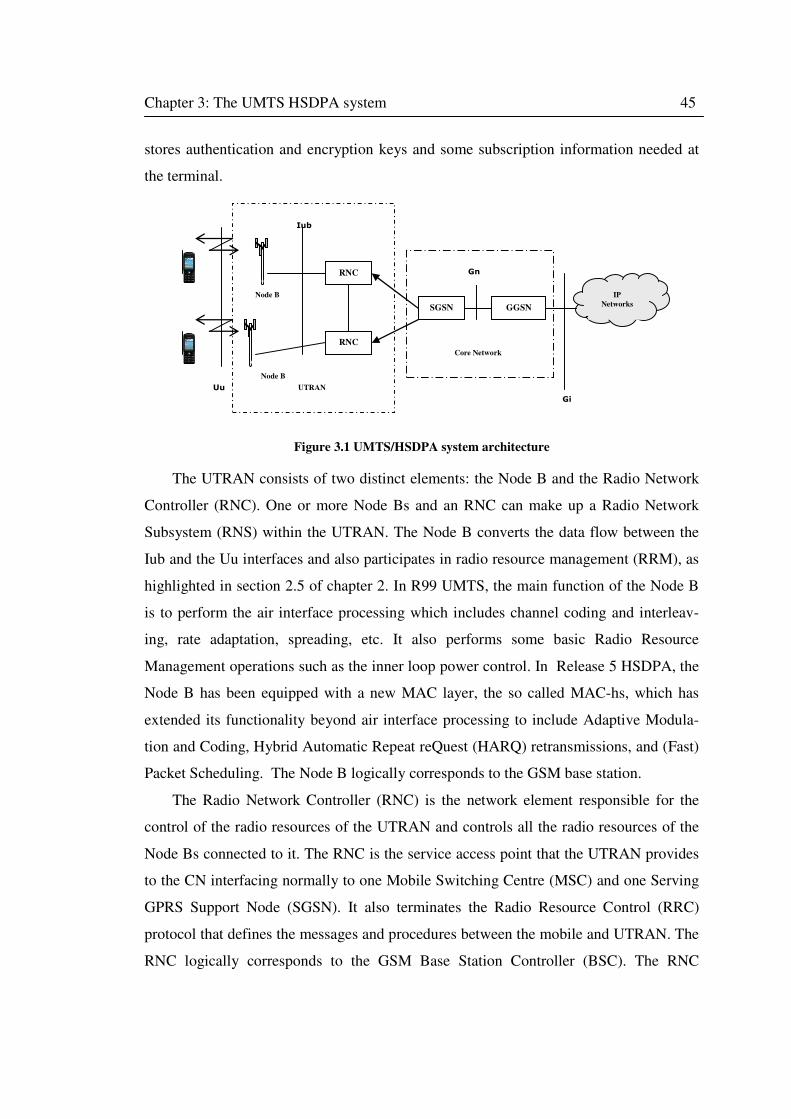
Chapter 3: The UMTS HSDPA system 45
stores authentication and encryption keys and some subscription information needed at
the terminal.
Uu
Node B
RNC
RNC
SGSN
Node B
UTRAN
Core Network
Gn
Iub
Node B
GGSN
Gi
IP
Networks
Figure 3.1 UMTS/HSDPA system architecture
The UTRAN consists of two distinct elements: the Node B and the Radio Network
Controller (RNC). One or more Node Bs and an RNC can make up a Radio Network
Subsystem (RNS) within the UTRAN. The Node B converts the data flow between the
Iub and the Uu interfaces and also participates in radio resource management (RRM), as
highlighted in section 2.5 of chapter 2. In R99 UMTS, the main function of the Node B
is to perform the air interface processing which includes channel coding and interleav-
ing, rate adaptation, spreading, etc. It also performs some basic Radio Resource
Management operations such as the inner loop power control. In Release 5 HSDPA, the
Node B has been equipped with a new MAC layer, the so called MAC-hs, which has
extended its functionality beyond air interface processing to include Adaptive Modula-
tion and Coding, Hybrid Automatic Repeat reQuest (HARQ) retransmissions, and (Fast)
Packet Scheduling. The Node B logically corresponds to the GSM base station.
The Radio Network Controller (RNC) is the network element responsible for the
control of the radio resources of the UTRAN and controls all the radio resources of the
Node Bs connected to it. The RNC is the service access point that the UTRAN provides
to the CN interfacing normally to one Mobile Switching Centre (MSC) and one Serving
GPRS Support Node (SGSN). It also terminates the Radio Resource Control (RRC)
protocol that defines the messages and procedures between the mobile and UTRAN. The
RNC logically corresponds to the GSM Base Station Controller (BSC). The RNC
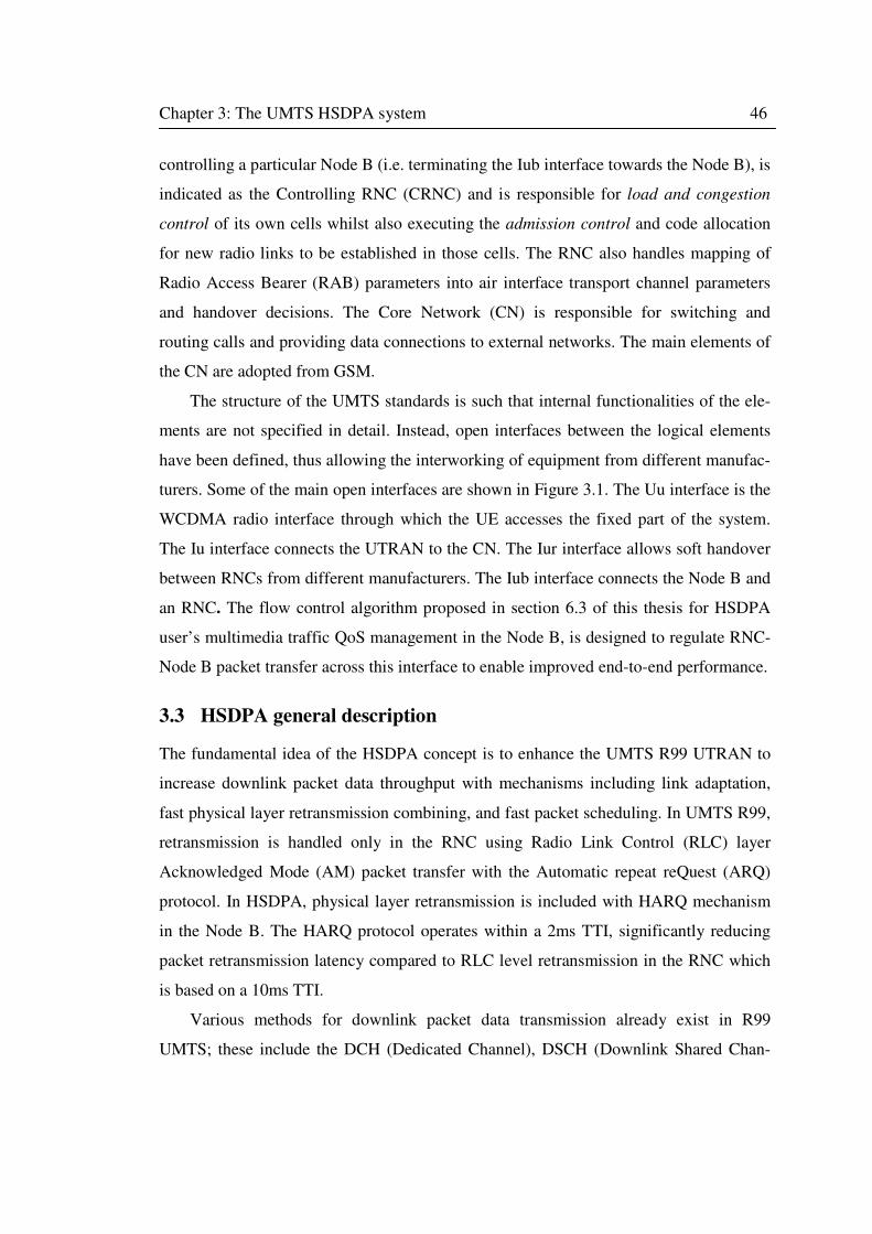
Chapter 3: The UMTS HSDPA system 46
controlling a particular Node B (i.e. terminating the Iub interface towards the Node B), is
indicated as the Controlling RNC (CRNC) and is responsible for load and congestion
control of its own cells whilst also executing the admission control and code allocation
for new radio links to be established in those cells. The RNC also handles mapping of
Radio Access Bearer (RAB) parameters into air interface transport channel parameters
and handover decisions. The Core Network (CN) is responsible for switching and
routing calls and providing data connections to external networks. The main elements of
the CN are adopted from GSM.
The structure of the UMTS standards is such that internal functionalities of the ele-
ments are not specified in detail. Instead, open interfaces between the logical elements
have been defined, thus allowing the interworking of equipment from different manufac-
turers. Some of the main open interfaces are shown in Figure 3.1. The Uu interface is the
WCDMA radio interface through which the UE accesses the fixed part of the system.
The Iu interface connects the UTRAN to the CN. The Iur interface allows soft handover
between RNCs from different manufacturers. The Iub interface connects the Node B and
an RNC. The flow control algorithm proposed in section 6.3 of this thesis for HSDPA
user’s multimedia traffic QoS management in the Node B, is designed to regulate RNC-
Node B packet transfer across this interface to enable improved end-to-end performance.
3.3 HSDPA general description
The fundamental idea of the HSDPA concept is to enhance the UMTS R99 UTRAN to
increase downlink packet data throughput with mechanisms including link adaptation,
fast physical layer retransmission combining, and fast packet scheduling. In UMTS R99,
retransmission is handled only in the RNC using Radio Link Control (RLC) layer
Acknowledged Mode (AM) packet transfer with the Automatic repeat reQuest (ARQ)
protocol. In HSDPA, physical layer retransmission is included with HARQ mechanism
in the Node B. The HARQ protocol operates within a 2ms TTI, significantly reducing
packet retransmission latency compared to RLC level retransmission in the RNC which
is based on a 10ms TTI.
Various methods for downlink packet data transmission already exist in R99
UMTS; these include the DCH (Dedicated Channel), DSCH (Downlink Shared Chan-
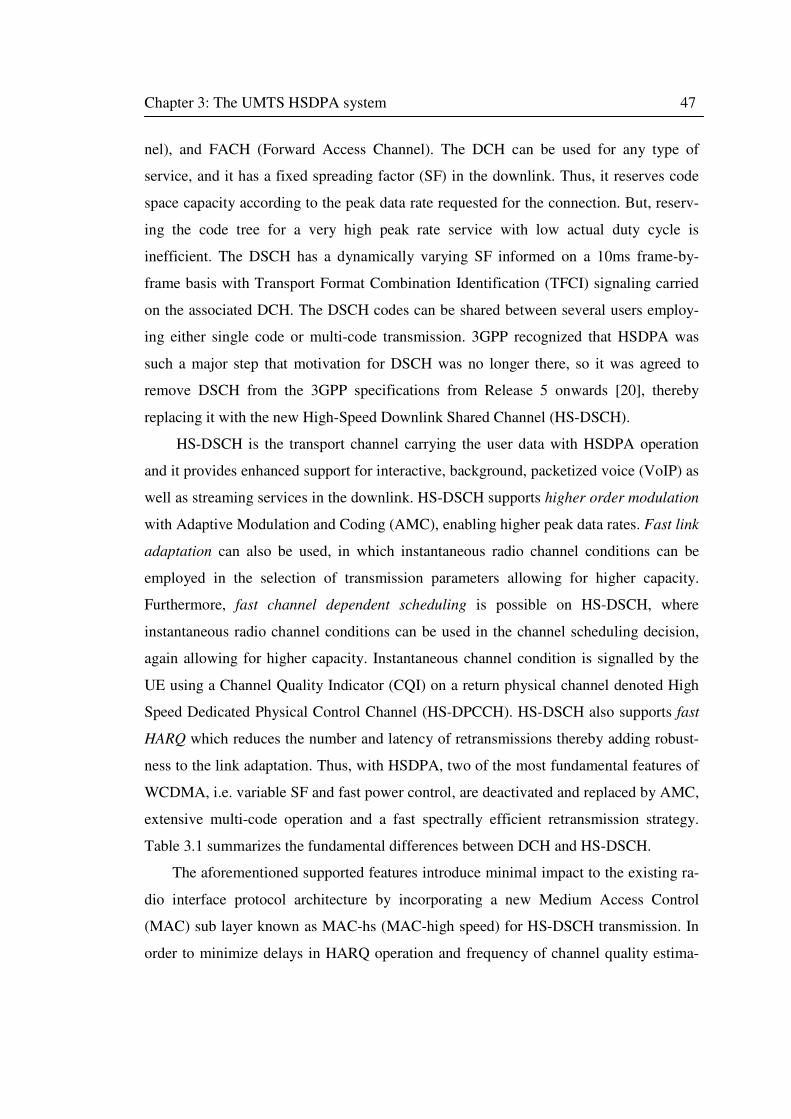
Chapter 3: The UMTS HSDPA system 47
nel), and FACH (Forward Access Channel). The DCH can be used for any type of
service, and it has a fixed spreading factor (SF) in the downlink. Thus, it reserves code
space capacity according to the peak data rate requested for the connection. But, reserv-
ing the code tree for a very high peak rate service with low actual duty cycle is
inefficient. The DSCH has a dynamically varying SF informed on a 10ms frame-by-
frame basis with Transport Format Combination Identification (TFCI) signaling carried
on the associated DCH. The DSCH codes can be shared between several users employ-
ing either single code or multi-code transmission. 3GPP recognized that HSDPA was
such a major step that motivation for DSCH was no longer there, so it was agreed to
remove DSCH from the 3GPP specifications from Release 5 onwards [20], thereby
replacing it with the new High-Speed Downlink Shared Channel (HS-DSCH).
HS-DSCH is the transport channel carrying the user data with HSDPA operation
and it provides enhanced support for interactive, background, packetized voice (VoIP) as
well as streaming services in the downlink. HS-DSCH supports higher order modulation
with Adaptive Modulation and Coding (AMC), enabling higher peak data rates. Fast link
adaptation can also be used, in which instantaneous radio channel conditions can be
employed in the selection of transmission parameters allowing for higher capacity.
Furthermore, fast channel dependent scheduling is possible on HS-DSCH, where
instantaneous radio channel conditions can be used in the channel scheduling decision,
again allowing for higher capacity. Instantaneous channel condition is signalled by the
UE using a Channel Quality Indicator (CQI) on a return physical channel denoted High
Speed Dedicated Physical Control Channel (HS-DPCCH). HS-DSCH also supports fast
HARQ which reduces the number and latency of retransmissions thereby adding robust-
ness to the link adaptation. Thus, with HSDPA, two of the most fundamental features of
WCDMA, i.e. variable SF and fast power control, are deactivated and replaced by AMC,
extensive multi-code operation and a fast spectrally efficient retransmission strategy.
Table 3.1 summarizes the fundamental differences between DCH and HS-DSCH.
The aforementioned supported features introduce minimal impact to the existing ra-
dio interface protocol architecture by incorporating a new Medium Access Control
(MAC) sub layer known as MAC-hs (MAC-high speed) for HS-DSCH transmission. In
order to minimize delays in HARQ operation and frequency of channel quality estima-
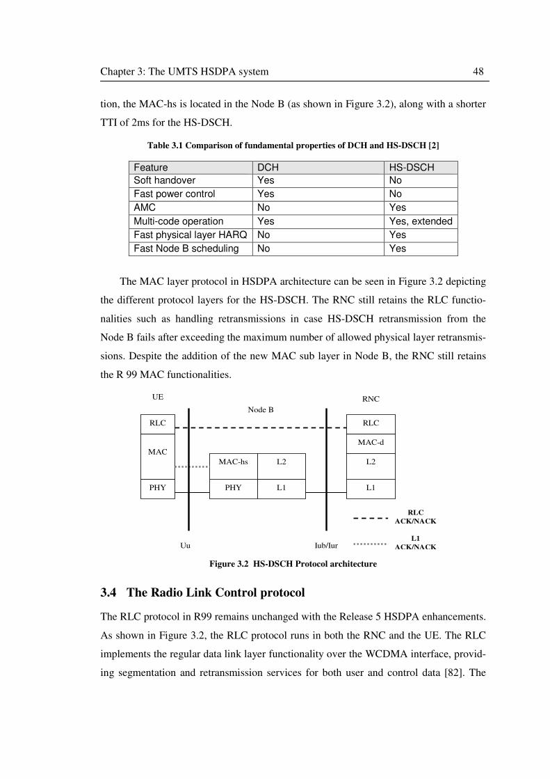
Chapter 3: The UMTS HSDPA system 48
tion, the MAC-hs is located in the Node B (as shown in Figure 3.2), along with a shorter
TTI of 2ms for the HS-DSCH.
Table 3.1 Comparison of fundamental properties of DCH and HS-DSCH [2]
Feature DCH HS-DSCH
Soft handover Yes No
Fast power control Yes No
AMC No Yes
Multi-code operation Yes Yes, extended
Fast physical layer HARQ No Yes
Fast Node B scheduling No Yes
The MAC layer protocol in HSDPA architecture can be seen in Figure 3.2 depicting
the different protocol layers for the HS-DSCH. The RNC still retains the RLC functio-
nalities such as handling retransmissions in case HS-DSCH retransmission from the
Node B fails after exceeding the maximum number of allowed physical layer retransmis-
sions. Despite the addition of the new MAC sub layer in Node B, the RNC still retains
the R 99 MAC functionalities.
RLC RLC
MAC
PHY PHY
MAC-hs L2
L1 L1
L2
MAC-d
Uu Iub/Iur
RLC
ACK/NACK
L1
ACK/NACK
UE
Node B
RNC
Figure 3.2 HS-DSCH Protocol architecture
3.4 The Radio Link Control protocol
The RLC protocol in R99 remains unchanged with the Release 5 HSDPA enhancements.
As shown in Figure 3.2, the RLC protocol runs in both the RNC and the UE. The RLC
implements the regular data link layer functionality over the WCDMA interface, provid-
ing segmentation and retransmission services for both user and control data [82]. The
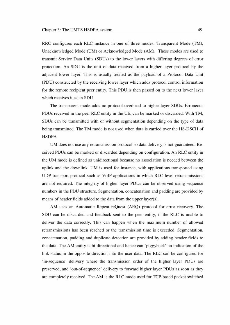
Chapter 3: The UMTS HSDPA system 49
RRC configures each RLC instance in one of three modes: Transparent Mode (TM),
Unacknowledged Mode (UM) or Acknowledged Mode (AM). These modes are used to
transmit Service Data Units (SDUs) to the lower layers with differing degrees of error
protection. An SDU is the unit of data received from a higher layer protocol by the
adjacent lower layer. This is usually treated as the payload of a Protocol Data Unit
(PDU) constructed by the receiving lower layer which adds protocol control information
for the remote recipient peer entity. This PDU is then passed on to the next lower layer
which receives it as an SDU.
The transparent mode adds no protocol overhead to higher layer SDUs. Erroneous
PDUs received in the peer RLC entity in the UE, can be marked or discarded. With TM,
SDUs can be transmitted with or without segmentation depending on the type of data
being transmitted. The TM mode is not used when data is carried over the HS-DSCH of
HSDPA.
UM does not use any retransmission protocol so data delivery is not guaranteed. Re-
ceived PDUs can be marked or discarded depending on configuration. An RLC entity in
the UM mode is defined as unidirectional because no association is needed between the
uplink and the downlink. UM is used for instance, with applications transported using
UDP transport protocol such as VoIP applications in which RLC level retransmissions
are not required. The integrity of higher layer PDUs can be observed using sequence
numbers in the PDU structure. Segmentation, concatenation and padding are provided by
means of header fields added to the data from the upper layer(s).
AM uses an Automatic Repeat reQuest (ARQ) protocol for error recovery. The
SDU can be discarded and feedback sent to the peer entity, if the RLC is unable to
deliver the data correctly. This can happen when the maximum number of allowed
retransmissions has been reached or the transmission time is exceeded. Segmentation,
concatenation, padding and duplicate detection are provided by adding header fields to
the data. The AM entity is bi-directional and hence can ‘piggyback’ an indication of the
link status in the opposite direction into the user data. The RLC can be configured for
‘in-sequence’ delivery where the transmission order of the higher layer PDUs are
preserved, and ‘out-of-sequence’ delivery to forward higher layer PDUs as soon as they
are completely received. The AM is the RLC mode used for TCP-based packet switched
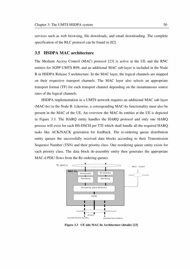
Chapter 3: The UMTS HSDPA system 50
services such as web browsing, file downloads, and email downloading. The complete
specification of the RLC protocol can be found in [82].
3.5 HSDPA MAC architecture
The Medium Access Control (MAC) protocol [23] is active at the UE and the RNC
entities for 3GPP UMTS R99, and an additional MAC sub-layer is included in the Node
B in HSDPA Release 5 architecture. In the MAC layer, the logical channels are mapped
on their respective transport channels. The MAC layer also selects an appropriate
transport format (TF) for each transport channel depending on the instantaneous source
rates of the logical channels.
HSDPA implementation in a UMTS network requires an additional MAC sub layer
(MAC-hs) in the Node B. Likewise, a corresponding MAC-hs functionality must also be
present in the MAC of the UE. An overview the MAC-hs entities at the UE is depicted
in Figure 3.3. The HARQ entity handles the HARQ protocol and only one HARQ
process will exist for each HS-DSCH per TTI which shall handle all the required HARQ
tasks like ACK/NACK generation for feedback. The re-ordering queue distribution
entity queues the successfully received data blocks according to their Transmission
Sequence Number (TSN) and their priority class. One reordering queue entity exists for
each priority class. The data block de-assembly entity then generates the appropriate
MAC-d PDU flows from the Re-ordering queues.
Figure 3.3 UE side MAC-hs Architecture (details) [23]
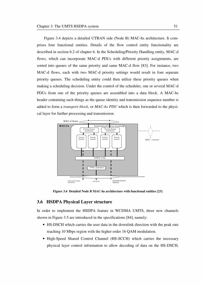
Chapter 3: The UMTS HSDPA system 51
Figure 3.4 depicts a detailed UTRAN side (Node B) MAC-hs architecture. It com-
prises four functional entities. Details of the flow control entity functionality are
described in section 6.2 of chapter 6. In the Scheduling/Priority Handling entity, MAC-d
flows, which can incorporate MAC-d PDUs with different priority assignments, are
sorted into queues of the same priority and same MAC-d flow [83]. For instance, two
MAC-d flows, each with two MAC-d priority settings would result in four separate
priority queues. The scheduling entity could then utilize these priority queues when
making a scheduling decision. Under the control of the scheduler, one or several MAC-d
PDUs from one of the priority queues are assembled into a data block. A MAC-hs
header containing such things as the queue identity and transmission sequence number is
added to form a transport block, or MAC-hs PDU which is then forwarded to the physi-
cal layer for further processing and transmission.
M AC -hs
M AC – C ontro l
HS-D SCH
TFRC selection
P riority Q ueued istribu tion
Associated DownlinkSignalling
Associated Up linkSignalling
M AC-d flows
HAR Q entity
P riority Q ueuedistribution
P rio rityQueue
PriorityQueue
P riorityQue ue
PriorityQueue
Scheduling/P riority handling
Associated Downlink
Signalling
Figure 3.4 Detailed Node B MAC-hs architecture with functional entities [23]
3.6 HSDPA Physical Layer structure
In order to implement the HSDPA feature in WCDMA UMTS, three new channels
shown in Figure 3.5 are introduced in the specifications [84], namely:
• HS-DSCH which carries the user data in the downlink direction with the peak rate
reaching 10 Mbps region with the higher order 16 QAM modulation.
• High-Speed Shared Control Channel (HS-SCCH) which carries the necessary
physical layer control information to allow decoding of data on the HS-DSCH,
Chapter 3: The UMTS HSDPA system 52
and enables possible physical layer combining of data sent on the HS-DSCH in
case of erroneous packet retransmission.
• Uplink High-Speed Dedicated Physical Control Channel (HS-DPCCH) which is
responsible for carrying the necessary control information on the uplink, namely
ACK/NACK information and downlink quality feedback information via the
Channel Quality Indicator (CQI) parameter.
UE
Node B
HS-SCCH
HS-DSCH
HS-DPCCH
Figure 3.5 The new channels introduced in release 5 for HSDPA operation
3.6.1 High-Speed Downlink Shared Channel
The HS-DSCH is characterized by a Transmission Time Interval (TTI) or interleaving
period of 2ms (three slots) to achieve a short round-trip delay for the operation between
the UE and the Node B, for retransmissions and channel quality feedback reporting. The
2ms TTI is short in comparison to the 10, 20, 40 or 80ms TTI sizes supported in R99.
Furthermore, adding a higher-order modulation scheme, 16 (Quadrature Amplitude
Modulation) QAM, and lower channel encoding redundancy enables increased instanta-
neous peak data rates. A fixed spreading factor (SF) of 16 is utilized, while multi-code
transmission with possible code multiplexing of different users is supported on the HS-
DSCH. The maximum number of codes that can be allocated with an SF of 16 is indeed
16, but due to the need for reserving code space for common channels, HS-SCCHs and
for the associated DCH, the maximum usable number of codes is set at 15. individual
terminals may receive a maximum of 5, 10, or 15 codes depending on their capability.
An example scenario where two users share the HS-DSCH is shown in Figure 3.6. Both
users check the information from the HS-SCCHs to determine which HS-DSCH codes to
despread as well as other parameters necessary for correct detection.
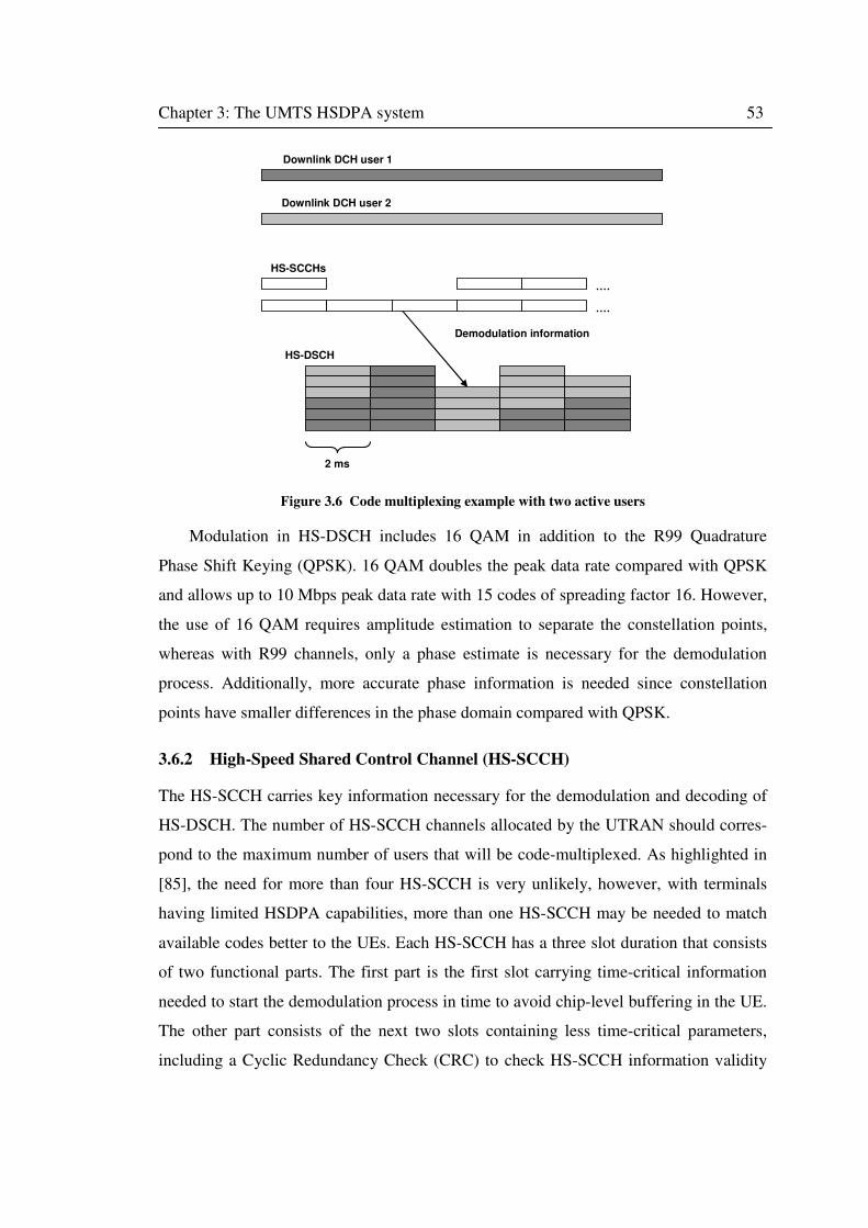
Chapter 3: The UMTS HSDPA system 53
Downlink DCH user 1
2 ms
HS-DSCH
HS-SCCHs
Downlink DCH user 2
Demodulation information
Figure 3.6 Code multiplexing example with two active users
Modulation in HS-DSCH includes 16 QAM in addition to the R99 Quadrature
Phase Shift Keying (QPSK). 16 QAM doubles the peak data rate compared with QPSK
and allows up to 10 Mbps peak data rate with 15 codes of spreading factor 16. However,
the use of 16 QAM requires amplitude estimation to separate the constellation points,
whereas with R99 channels, only a phase estimate is necessary for the demodulation
process. Additionally, more accurate phase information is needed since constellation
points have smaller differences in the phase domain compared with QPSK.
3.6.2 High-Speed Shared Control Channel (HS-SCCH)
The HS-SCCH carries key information necessary for the demodulation and decoding of
HS-DSCH. The number of HS-SCCH channels allocated by the UTRAN should corres-
pond to the maximum number of users that will be code-multiplexed. As highlighted in
[85], the need for more than four HS-SCCH is very unlikely, however, with terminals
having limited HSDPA capabilities, more than one HS-SCCH may be needed to match
available codes better to the UEs. Each HS-SCCH has a three slot duration that consists
of two functional parts. The first part is the first slot carrying time-critical information
needed to start the demodulation process in time to avoid chip-level buffering in the UE.
The other part consists of the next two slots containing less time-critical parameters,
including a Cyclic Redundancy Check (CRC) to check HS-SCCH information validity
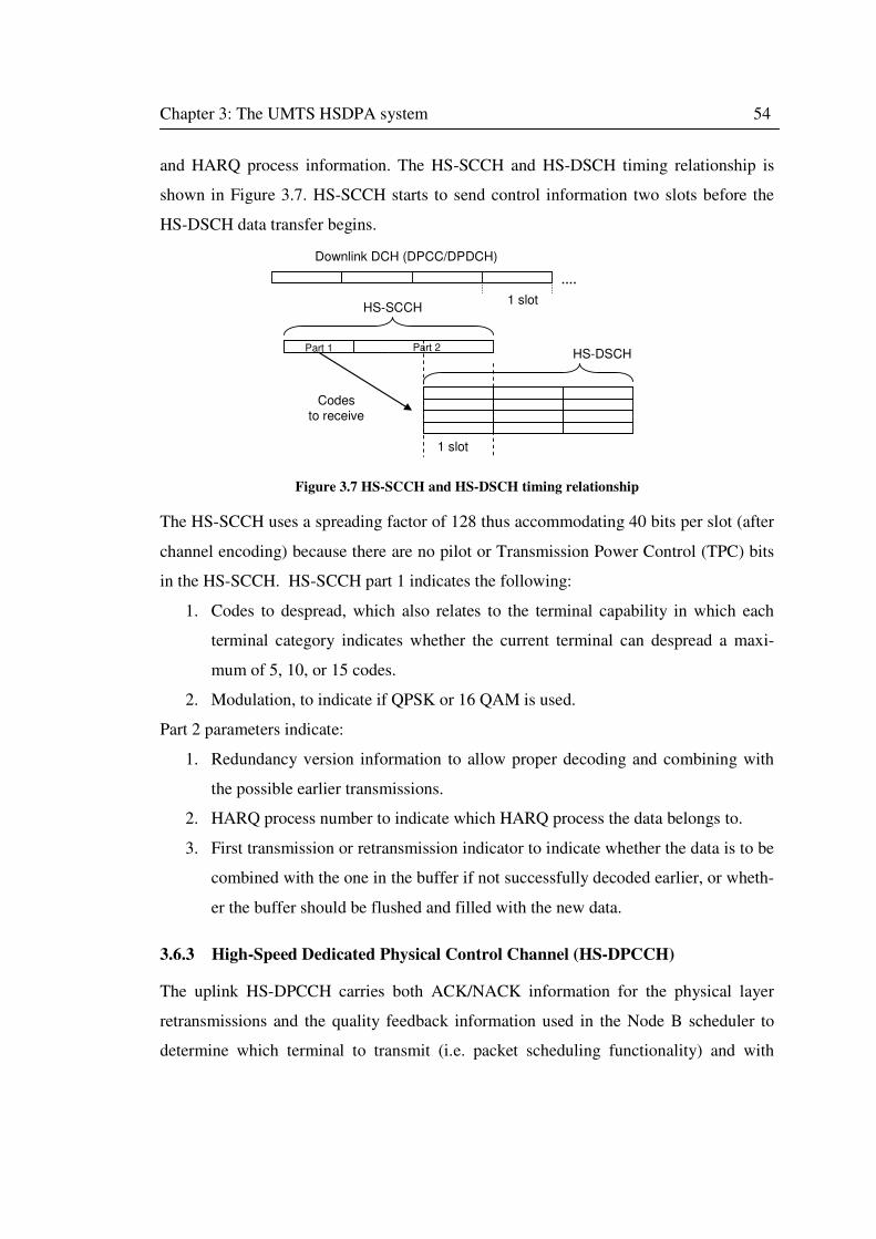
Chapter 3: The UMTS HSDPA system 54
and HARQ process information. The HS-SCCH and HS-DSCH timing relationship is
shown in Figure 3.7. HS-SCCH starts to send control information two slots before the
HS-DSCH data transfer begins.
Downlink DCH (DPCC/DPDCH)
1 slot
1 slot
HS-SCCH
HS-DSCH
Codesto receive
Part 1 Part 2
Figure 3.7 HS-SCCH and HS-DSCH timing relationship
The HS-SCCH uses a spreading factor of 128 thus accommodating 40 bits per slot (after
channel encoding) because there are no pilot or Transmission Power Control (TPC) bits
in the HS-SCCH. HS-SCCH part 1 indicates the following:
1. Codes to despread, which also relates to the terminal capability in which each
terminal category indicates whether the current terminal can despread a maxi-
mum of 5, 10, or 15 codes.
2. Modulation, to indicate if QPSK or 16 QAM is used.
Part 2 parameters indicate:
1. Redundancy version information to allow proper decoding and combining with
the possible earlier transmissions.
2. HARQ process number to indicate which HARQ process the data belongs to.
3. First transmission or retransmission indicator to indicate whether the data is to be
combined with the one in the buffer if not successfully decoded earlier, or wheth-
er the buffer should be flushed and filled with the new data.
3.6.3 High-Speed Dedicated Physical Control Channel (HS-DPCCH)
The uplink HS-DPCCH carries both ACK/NACK information for the physical layer
retransmissions and the quality feedback information used in the Node B scheduler to
determine which terminal to transmit (i.e. packet scheduling functionality) and with
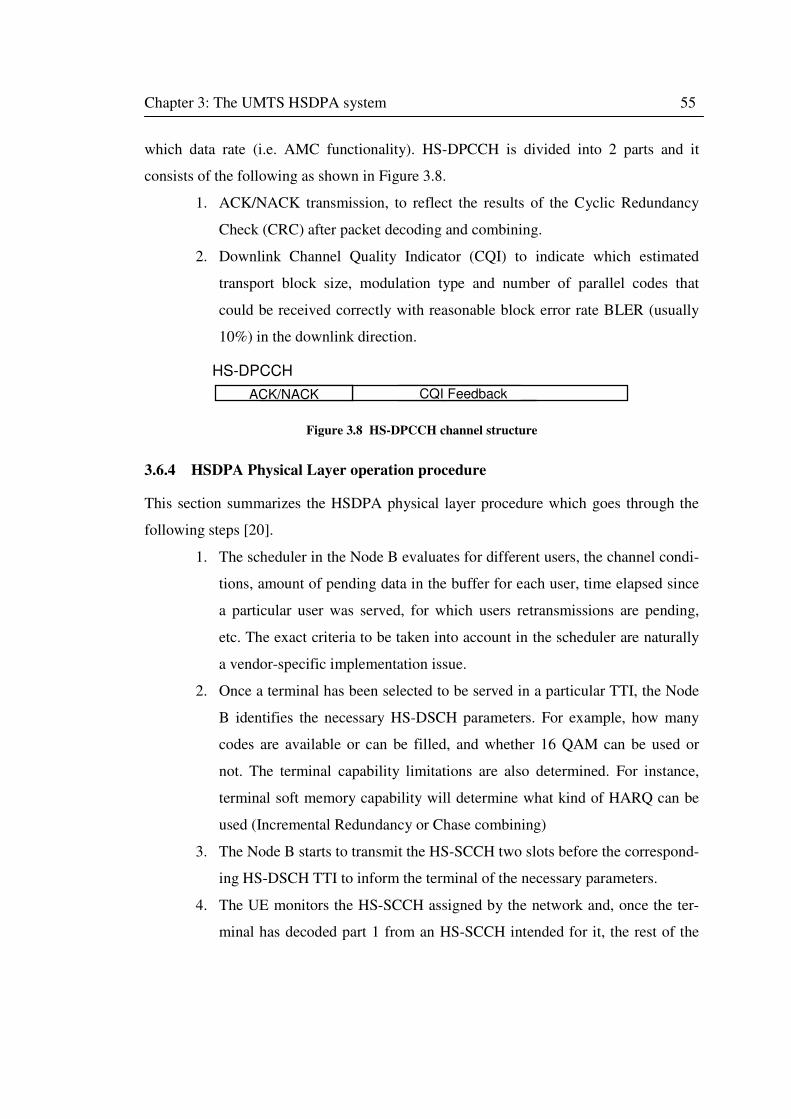
Chapter 3: The UMTS HSDPA system 55
which data rate (i.e. AMC functionality). HS-DPCCH is divided into 2 parts and it
consists of the following as shown in Figure 3.8.
1. ACK/NACK transmission, to reflect the results of the Cyclic Redundancy
Check (CRC) after packet decoding and combining.
2. Downlink Channel Quality Indicator (CQI) to indicate which estimated
transport block size, modulation type and number of parallel codes that
could be received correctly with reasonable block error rate BLER (usually
10%) in the downlink direction.
HS-DPCCH
ACK/NACK CQI Feedback
Figure 3.8 HS-DPCCH channel structure
3.6.4 HSDPA Physical Layer operation procedure
This section summarizes the HSDPA physical layer procedure which goes through the
following steps [20].
1. The scheduler in the Node B evaluates for different users, the channel condi-
tions, amount of pending data in the buffer for each user, time elapsed since
a particular user was served, for which users retransmissions are pending,
etc. The exact criteria to be taken into account in the scheduler are naturally
a vendor-specific implementation issue.
2. Once a terminal has been selected to be served in a particular TTI, the Node
B identifies the necessary HS-DSCH parameters. For example, how many
codes are available or can be filled, and whether 16 QAM can be used or
not. The terminal capability limitations are also determined. For instance,
terminal soft memory capability will determine what kind of HARQ can be
used (Incremental Redundancy or Chase combining)
3. The Node B starts to transmit the HS-SCCH two slots before the correspond-
ing HS-DSCH TTI to inform the terminal of the necessary parameters.
4. The UE monitors the HS-SCCH assigned by the network and, once the ter-
minal has decoded part 1 from an HS-SCCH intended for it, the rest of the
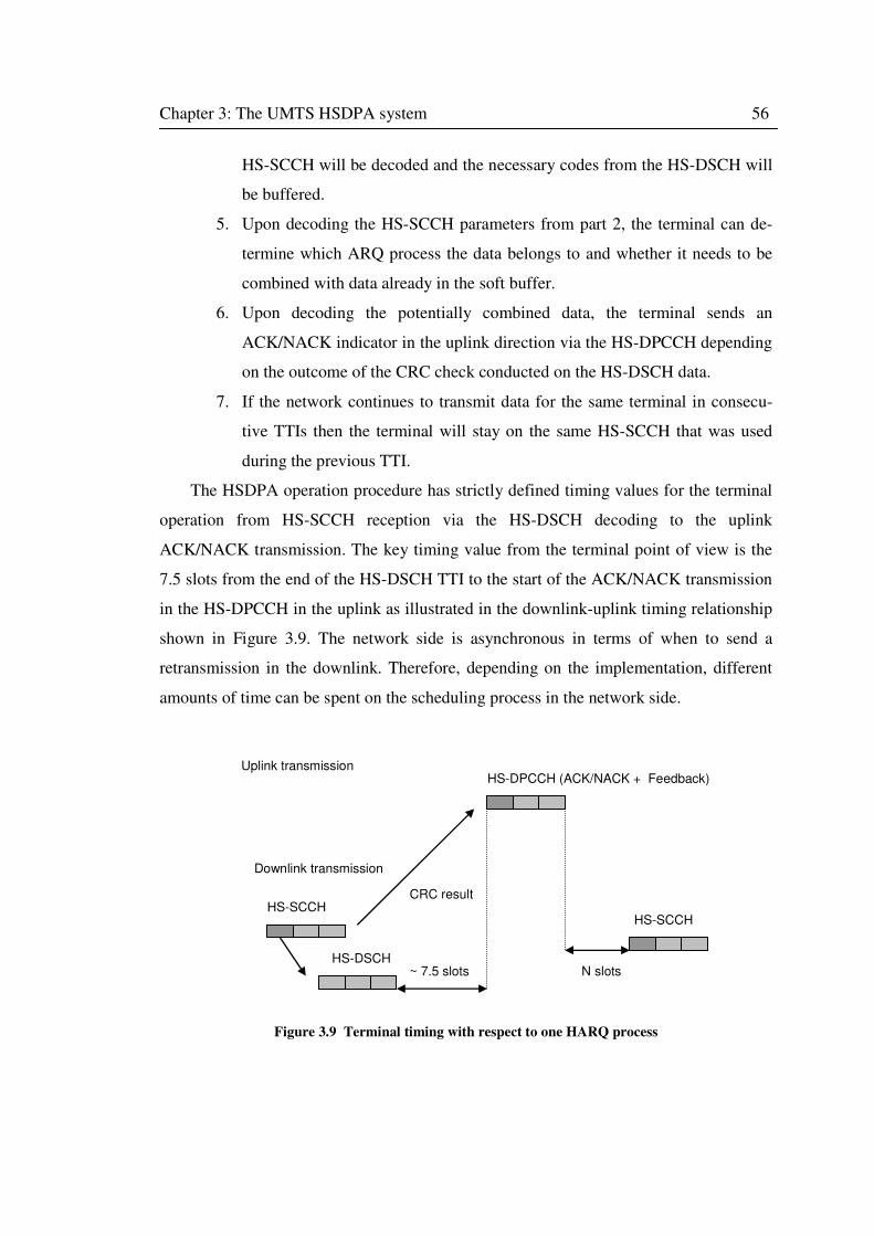
Chapter 3: The UMTS HSDPA system 56
HS-SCCH will be decoded and the necessary codes from the HS-DSCH will
be buffered.
5. Upon decoding the HS-SCCH parameters from part 2, the terminal can de-
termine which ARQ process the data belongs to and whether it needs to be
combined with data already in the soft buffer.
6. Upon decoding the potentially combined data, the terminal sends an
ACK/NACK indicator in the uplink direction via the HS-DPCCH depending
on the outcome of the CRC check conducted on the HS-DSCH data.
7. If the network continues to transmit data for the same terminal in consecu-
tive TTIs then the terminal will stay on the same HS-SCCH that was used
during the previous TTI.
The HSDPA operation procedure has strictly defined timing values for the terminal
operation from HS-SCCH reception via the HS-DSCH decoding to the uplink
ACK/NACK transmission. The key timing value from the terminal point of view is the
7.5 slots from the end of the HS-DSCH TTI to the start of the ACK/NACK transmission
in the HS-DPCCH in the uplink as illustrated in the downlink-uplink timing relationship
shown in Figure 3.9. The network side is asynchronous in terms of when to send a
retransmission in the downlink. Therefore, depending on the implementation, different
amounts of time can be spent on the scheduling process in the network side.
HS-DSCH
HS-SCCH
N slots
HS-DPCCH (ACK/NACK + Feedback)
~ 7.5 slots
CRC result
Uplink transmission
Downlink transmission
HS-SCCH
Figure 3.9 Terminal timing with respect to one HARQ process
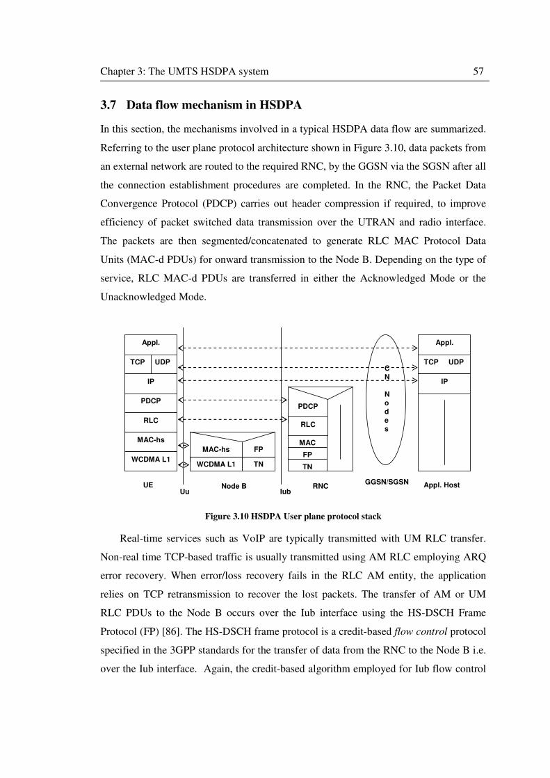
Chapter 3: The UMTS HSDPA system 57
3.7 Data flow mechanism in HSDPA
In this section, the mechanisms involved in a typical HSDPA data flow are summarized.
Referring to the user plane protocol architecture shown in Figure 3.10, data packets from
an external network are routed to the required RNC, by the GGSN via the SGSN after all
the connection establishment procedures are completed. In the RNC, the Packet Data
Convergence Protocol (PDCP) carries out header compression if required, to improve
efficiency of packet switched data transmission over the UTRAN and radio interface.
The packets are then segmented/concatenated to generate RLC MAC Protocol Data
Units (MAC-d PDUs) for onward transmission to the Node B. Depending on the type of
service, RLC MAC-d PDUs are transferred in either the Acknowledged Mode or the
Unacknowledged Mode.
Appl.
TCP UDP
IP
PDCP
RLC
MAC-hs
WCDMA L1WCDMA L1
MAC-hs
TN
FP
RLC
PDCP
TN
FP
MAC
Appl.
TCP UDP
IP
GGSN/SGSN
Uu IubUE RNC Appl. HostNode B
C
N
N
o
d
e
s
Figure 3.10 HSDPA User plane protocol stack
Real-time services such as VoIP are typically transmitted with UM RLC transfer.
Non-real time TCP-based traffic is usually transmitted using AM RLC employing ARQ
error recovery. When error/loss recovery fails in the RLC AM entity, the application
relies on TCP retransmission to recover the lost packets. The transfer of AM or UM
RLC PDUs to the Node B occurs over the Iub interface using the HS-DSCH Frame
Protocol (FP) [86]. The HS-DSCH frame protocol is a credit-based flow control protocol
specified in the 3GPP standards for the transfer of data from the RNC to the Node B i.e.
over the Iub interface. Again, the credit-based algorithm employed for Iub flow control
Chapter 3: The UMTS HSDPA system 58
in practice is a vendor-specific issue. However, the flow control mechanism is aimed at
controlling the amount of user data buffered in the MAC-hs (of the Node B ready for
scheduling on the HS-DSCH) to prevent buffer overflow. In the Iub flow control, the
Node B issues credits to the RNC through the CAPACITY ALLOCATION FP control
frame on receipt of a CAPACITY REQUEST FP control frame from the RNC. The
number of credits issued corresponds to the number of RLC MAC-d PDUs belonging to
a particular flow of a given user to be transferred; thus, the RNC packs the MAC-d
PDUs into 10ms HS-DSCH frames to be transmitted to the Node B. The enhanced buffer
management schemes proposed in this thesis are designed to exploit these Iub mecha-
nisms in their incorporated credit-based flow control algorithm.
On arrival of the HS-DSCH frames carrying the RLC PDUs to the Node B MAC-hs,
the RLC MAC-d PDUs are retrieved and queued in the MAC-hs buffer to await trans-
mission. When the packet scheduler assigns a transmission slot to the UE, one or several
MAC-d PDUs from its queue(s) are assembled into a data block or MAC-hs PDU. A
MAC-hs header containing the queue identity, and transmission sequence number etc., is
added to form a MAC-hs PDU or Transport Block which is then forwarded to the
physical layer for further processing. Recall that the Transport Block Size and hence
number of MAC-d PDUs transmitted will depend on the selected AMC schemes and the
number of channelization codes, which will be chosen according to the CQI that ex-
presses the last known UE channel conditions. A HARQ process is assigned for the
transmission of a transport block to the UE in the allocated TTI, and the Transmission
Sequence Number (TSN) in the frame is used to preserve the integrity and the order of
the data.
On arrival at the UE, a peer HARQ entity receives the data frame and sends an ACK
if decoding was successful or a NACK otherwise. The reverse feedback channel, HS-
DPCCH is used to carry the HARQ ACK/NACK as well as the CQI that is used in AMC
scheme selection. Correctly received frames are de-assembled into MAC-hs PDUs and
reordered in the MAC-hs reordering queues (c.f. Figure 3.3). The MAC-d PDUs are
extracted and sent to the RLC layer for further processing. A peer RLC AM entity will
send a STATUS PDU in the return direction if a POLL bit has been set in the header of
the received PDUs. The packets are reconstructed from the RLC PDUs and passed to the
Chapter 3: The UMTS HSDPA system 59
higher layer transport protocol for further processing and onward transfer to the applica-
tion layer.
All the above described mechanisms are either explicitly or implicitly modelled in
our system-level HSDPA simulator used to evaluate the end-to-end performance of E-
TSP and D-TSP buffer management schemes in chapters 6 and 7 respectively.
3.8 Chapter summary
This chapter provided background coverage of the UMTS system, with emphasis on the
downlink enhancement to the UTRAN, the so-called High Speed Downlink Packet
Access (HSDPA) introduced in 3GPP Release 5. The information presented here pre-
cedes the modelling and analyses of the HSDPA buffer management schemes presented
in this thesis, in order to put the proposed schemes into proper context. The
UMTS/HSDPA system architecture and the interacting entities, as well as protocol
architecture and the various layers and services provided have been described. The
supporting technologies of HSDPA that enable higher data rates, higher capacity, and
improved spectrum efficiency in UMTS systems; such as Adaptive Modulation and
Coding, fast HARQ, fast Packet Scheduling and their key mechanisms have also been
discussed. Finally, typical data flow procedures in a HSDPA system, which are implicit-
ly or explicitly replicated in the model designed and developed for simulation and
performance evaluation of the proposed HSDPA buffer management schemes in chap-
ters 6 and 7, are described.
The next chapter will discuss the novel Time Space Priority (TSP) queuing system,
and evaluate its performance using analytical methods with validation by discrete event
simulation. The chapter also presents a comparative analysis with the conventional
priority queuing disciplines discussed in chapter 2.
60
Chapter 4
The Time Space Priority Queuing
System
4.1 Introduction
Buffer allocation to provide an efficient and fair use of available resources is critically
important for multiplexed services comprising flows with diverse QoS requirements.
Current and future mobile networks will be able to support a broad spectrum of services,
including voice, video, image, data, etc. and multiplexed services or multimedia sessions
consisting of combinations of these. To make efficient use of network resources, it is
necessary that different types of services statistically share the network resources, such
as, the transmission capacity and buffer spaces. Different traffic types may have differ-
ent quality of service (QoS) requirements. Satisfaction of the different QoS requirements
is a resource allocation problem [87-89]. Hence, the work in this thesis is concerned with
buffer allocation problem for multiplexed services at the wireless interface of high speed
downlink packet access mobile networks.
This chapter introduces a novel Time-Space Priority queuing system for packet-
switched downlink heterogeneous multimedia traffic in mobile cellular radio access
networks (RAN), and presents analytical models for its performance evaluation.
In this chapter, TSP queuing is introduced and discussed first, followed by devel-
opment of Markov modelling of a (RAN base station) node with a single common
shared channel employing TSP queuing for downlink multimedia traffic composed of
real-time (RT) and non-real-time (NRT) flows, being transmitted concurrently to a user
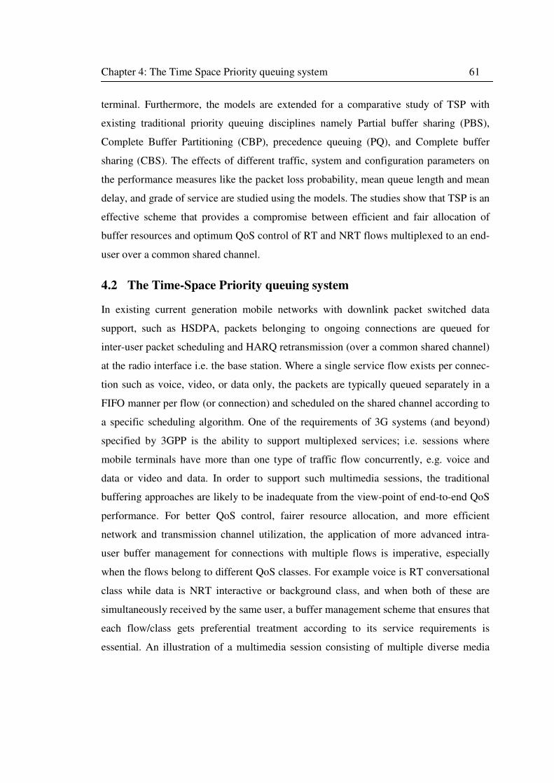
Chapter 4: The Time Space Priority queuing system 61
terminal. Furthermore, the models are extended for a comparative study of TSP with
existing traditional priority queuing disciplines namely Partial buffer sharing (PBS),
Complete Buffer Partitioning (CBP), precedence queuing (PQ), and Complete buffer
sharing (CBS). The effects of different traffic, system and configuration parameters on
the performance measures like the packet loss probability, mean queue length and mean
delay, and grade of service are studied using the models. The studies show that TSP is an
effective scheme that provides a compromise between efficient and fair allocation of
buffer resources and optimum QoS control of RT and NRT flows multiplexed to an end-
user over a common shared channel.
4.2 The Time-Space Priority queuing system
In existing current generation mobile networks with downlink packet switched data
support, such as HSDPA, packets belonging to ongoing connections are queued for
inter-user packet scheduling and HARQ retransmission (over a common shared channel)
at the radio interface i.e. the base station. Where a single service flow exists per connec-
tion such as voice, video, or data only, the packets are typically queued separately in a
FIFO manner per flow (or connection) and scheduled on the shared channel according to
a specific scheduling algorithm. One of the requirements of 3G systems (and beyond)
specified by 3GPP is the ability to support multiplexed services; i.e. sessions where
mobile terminals have more than one type of traffic flow concurrently, e.g. voice and
data or video and data. In order to support such multimedia sessions, the traditional
buffering approaches are likely to be inadequate from the view-point of end-to-end QoS
performance. For better QoS control, fairer resource allocation, and more efficient
network and transmission channel utilization, the application of more advanced intra-
user buffer management for connections with multiple flows is imperative, especially
when the flows belong to different QoS classes. For example voice is RT conversational
class while data is NRT interactive or background class, and when both of these are
simultaneously received by the same user, a buffer management scheme that ensures that
each flow/class gets preferential treatment according to its service requirements is
essential. An illustration of a multimedia session consisting of multiple diverse media
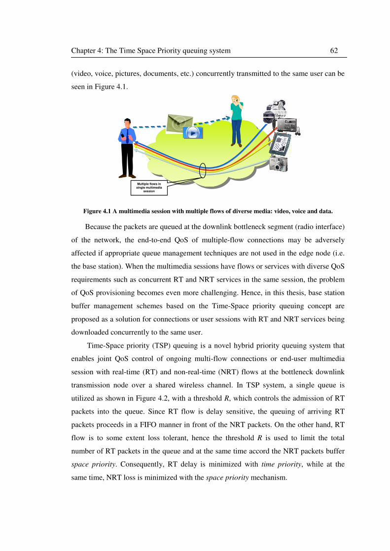
Chapter 4: The Time Space Priority queuing system 62
(video, voice, pictures, documents, etc.) concurrently transmitted to the same user can be
seen in Figure 4.1.
Multiple flows in single multimedia
session
Figure 4.1 A multimedia session with multiple flows of diverse media: video, voice and data.
Because the packets are queued at the downlink bottleneck segment (radio interface)
of the network, the end-to-end QoS of multiple-flow connections may be adversely
affected if appropriate queue management techniques are not used in the edge node (i.e.
the base station). When the multimedia sessions have flows or services with diverse QoS
requirements such as concurrent RT and NRT services in the same session, the problem
of QoS provisioning becomes even more challenging. Hence, in this thesis, base station
buffer management schemes based on the Time-Space priority queuing concept are
proposed as a solution for connections or user sessions with RT and NRT services being
downloaded concurrently to the same user.
Time-Space priority (TSP) queuing is a novel hybrid priority queuing system that
enables joint QoS control of ongoing multi-flow connections or end-user multimedia
session with real-time (RT) and non-real-time (NRT) flows at the bottleneck downlink
transmission node over a shared wireless channel. In TSP system, a single queue is
utilized as shown in Figure 4.2, with a threshold R, which controls the admission of RT
packets into the queue. Since RT flow is delay sensitive, the queuing of arriving RT
packets proceeds in a FIFO manner in front of the NRT packets. On the other hand, RT
flow is to some extent loss tolerant, hence the threshold R is used to limit the total
number of RT packets in the queue and at the same time accord the NRT packets buffer
space priority. Consequently, RT delay is minimized with time priority, while at the
same time, NRT loss is minimized with the space priority mechanism.

Chapter 4: The Time Space Priority queuing system 63
Note that with TSP queuing, the entire allocated buffer space is completely shared
by RT and NRT packets in spite of the threshold R. Hence, the total number of NRT
packets allowed in the buffer can range from N, the total queue capacity, to N-R, which
further minimizes loss of NRT packets. The complete sharing of the buffer space by both
classes also ensures high buffer utilization and results in lower overall packet loss
probability compared to non-sharing (i.e. complete partitioning policy). Furthermore,
NRT packet loss minimization in the base station buffer results in better network re-
source utilization and improves the performance of higher layer protocols, because lost
NRT packets typically must be retransmitted by means of (higher layer protocol) error
control mechanisms with consequent degradation in end-to-end throughput and waste of
transmission resources.
NBuffer capacity
Transmission to user terminal
RTime-Space
priority threshold
RT flow(Time priority)
NRT flow
(Space Priority)Service process
Figure 4.2 The Time-Space Priority queuing mechanism
Another important feature of the TSP queuing strategy is that RT packets assume a
limited ‘higher space priority’ up to the threshold limit R, at instances when a full buffer
is encountered by an arriving RT packet. This is achieved by implementing a Last in
First Drop (LIFD) policy where the packet at the tail of the (NRT) queue is dropped to
admit the arriving RT packet that meets a full buffer, as long as the total number of RT
packets in the TSP buffer is less than the threshold R. Note that the effect of this ‘LIFD
displacement’ policy is expected to give only a slight increase in overall NRT loss if the
threshold R is small in comparison to the total TSP buffer size N.
The effect of time priorities in TSP is to decrease the delay of the RT traffic at the
expense of the delay of the NRT traffic, and conversely, the effect of the space priorities
is to decrease the loss of NRT packets at the expense of the potential loss of RT packets
within acceptable limits (bounded by the threshold, R). The diverse QoS characteristics
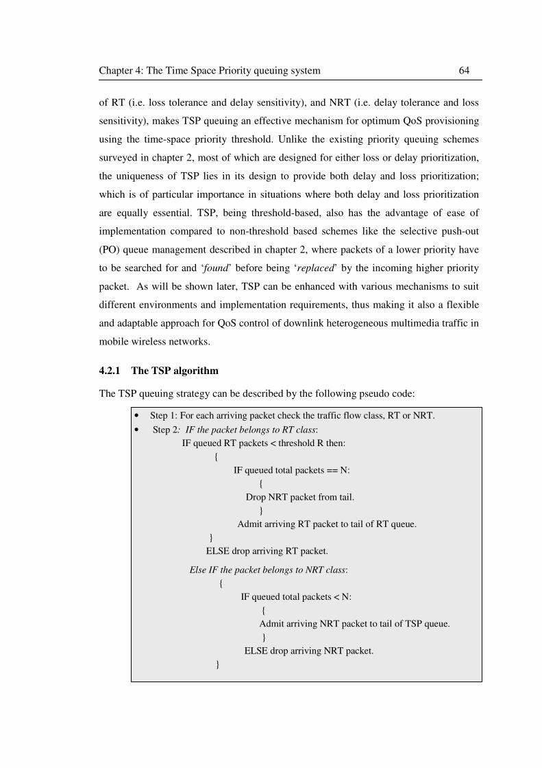
Chapter 4: The Time Space Priority queuing system 64
of RT (i.e. loss tolerance and delay sensitivity), and NRT (i.e. delay tolerance and loss
sensitivity), makes TSP queuing an effective mechanism for optimum QoS provisioning
using the time-space priority threshold. Unlike the existing priority queuing schemes
surveyed in chapter 2, most of which are designed for either loss or delay prioritization,
the uniqueness of TSP lies in its design to provide both delay and loss prioritization;
which is of particular importance in situations where both delay and loss prioritization
are equally essential. TSP, being threshold-based, also has the advantage of ease of
implementation compared to non-threshold based schemes like the selective push-out
(PO) queue management described in chapter 2, where packets of a lower priority have
to be searched for and ‘found’ before being ‘replaced’ by the incoming higher priority
packet. As will be shown later, TSP can be enhanced with various mechanisms to suit
different environments and implementation requirements, thus making it also a flexible
and adaptable approach for QoS control of downlink heterogeneous multimedia traffic in
mobile wireless networks.
4.2.1 The TSP algorithm
The TSP queuing strategy can be described by the following pseudo code:
• Step 1: For each arriving packet check the traffic flow class, RT or NRT.
• Step 2: IF the packet belongs to RT class:
IF queued RT packets < threshold R then:
{
IF queued total packets == N:
{
Drop NRT packet from tail.
}
Admit arriving RT packet to tail of RT queue.
}
ELSE drop arriving RT packet.
Else IF the packet belongs to NRT class:
{
IF queued total packets < N:
{
Admit arriving NRT packet to tail of TSP queue.
}
ELSE drop arriving NRT packet.
}
Chapter 4: The Time Space Priority queuing system 65
4.3 Formulation of TSP analytical model
This section presents the formulation of analytical models for investigating TSP perfor-
mance. The primary goal is to undertake initial analysis in this chapter to gain insight
into the impact of various system, traffic and configuration parameters on TSP perfor-
mance; and also, to perform comparative analysis with conventional types of priority
queuing schemes. Hence, in order to derive analytically tractable models, simplified
system and traffic assumptions sufficient to allow initial in-depth analyses of TSP are
employed in order to comprehend the behaviour of the TSP mechanism under various
conditions.
The results in this chapter have been generated using MOSEL-2 [90], the revised
version of MOSEL [91] (Modelling, Specification and Evaluation Language), an analyt-
ical modelling tool which incorporates a textual computer language for the description of
stochastic dynamic models and performance measures that result from such models.
With MOSEL-2, complex systems such as communication networks, computer systems,
production lines and many more can be modelled and analyzed. MOSEL translates
system description written in MOSEL language into the modelling languages of the tool
SPNP [92], a Stochastic Petri Net Package, and MOSES [93], a Markov analyzer. The
revised version, MOSEL-2, also provides translation into the TimeNET’s [94] modelling
language. The modelling environment MOSEL, not only translates the MOSEL descrip-
tions into the languages appropriate for the different tools, but also starts the tool
automatically, captures the computed results, and presents them in graphical form using
the Intermediate Graphical Language (IGL) described in [91]. Several papers can be
found where MOSEL is applied in performance and reliability modelling such as [95].
Some examples of MOSEL application in performance modelling and analysis of
communication systems can be found in [96], [97],[98], and [99].
4.3.1 Basic system modelling assumptions
Assuming that a network node, say a downlink base station buffer employing the TSP
queuing mechanism illustrated Figure 4.1, is modelled as an M2/M2/1/R, N queue. The
following features and assumptions characterize the system model:
Chapter 4: The Time Space Priority queuing system 66
� A receiver end user terminal maintains a session or connection comprising two
classes of flows; a real-time (RT) flow and a non-real-time (NRT) flow with in-
dependent packet arrivals to the base station buffer.
• The packets are queued according to the described TSP mechanism in a single
(logical) queue of limited capacity N for the connection.
� Packets are transmitted on a common downlink shared channel in a non-
preemptive manner. Thus, an arriving RT packet for example, cannot pre-empt
an NRT packet being transmitted.
� The times between packet arrivals are independent and exponentially distributed
with mean inter-arrival times 1/λrt and 1/λnrt for RT and NRT flows respectively.
� Packet transmission times are assumed to be independent and exponentially dis-
tributed with mean 1/µ rt and 1/µnrt and priority transmission on the next
transmission opportunity given to RT packets whenever both types are present in
the buffer.
4.3.2 Analytical model
In order to develop a Markov model for the system, we assume that the state of the
network at any given instant in time t is jointly described by the following:
� Number of RT packets in the base station single-user multimedia buffer queue.
� Number of NRT packets in the base station single-user multimedia buffer queue.
� Head-of-line packet waiting for transmission on the downlink channel from the
buffer at time t being RT.
� Head-of-line packet waiting for transmission on the downlink from the buffer
channel at time t being NRT.
Hence we define the state of the queuing system by a vector:
X = (r, n, p, q),
Where r is the number of RT packets present in the queue, n is the number of NRT
packets present in the queue, p is equal to 1 when the head-of-line (HOL) packet is RT
and 0 otherwise. Similarly, q denotes head-of-line status for NRT and is equal to 1 when
NRT is at the head and 0 otherwise, as depicted in Figure 4.3. Note the necessity to have
both p and q denoting the two head-of-line states, since instances when the queue is
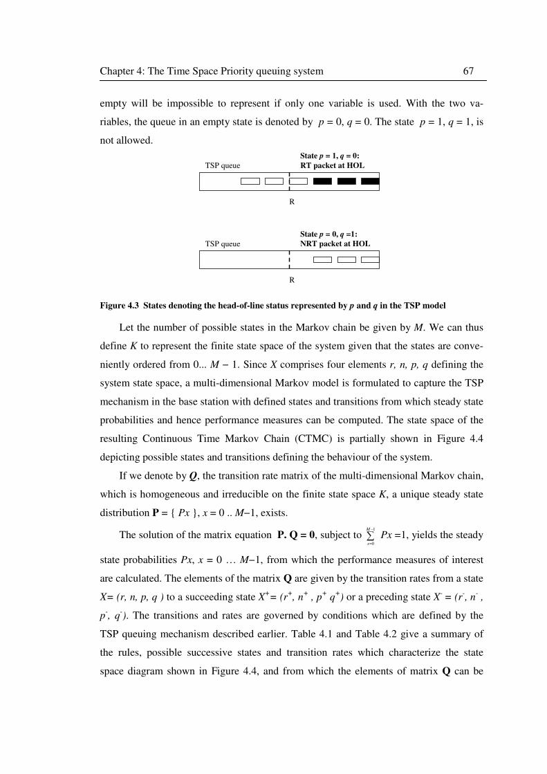
Chapter 4: The Time Space Priority queuing system 67
empty will be impossible to represent if only one variable is used. With the two va-
riables, the queue in an empty state is denoted by p = 0, q = 0. The state p = 1, q = 1, is
not allowed.
State p = 0, q =1:
NRT packet at HOL
State p = 1, q = 0:
RT packet at HOL
TSP queue
TSP queue
R
R
Figure 4.3 States denoting the head-of-line status represented by p and q in the TSP model
Let the number of possible states in the Markov chain be given by M. We can thus
define K to represent the finite state space of the system given that the states are conve-
niently ordered from 0... M − 1. Since X comprises four elements r, n, p, q defining the
system state space, a multi-dimensional Markov model is formulated to capture the TSP
mechanism in the base station with defined states and transitions from which steady state
probabilities and hence performance measures can be computed. The state space of the
resulting Continuous Time Markov Chain (CTMC) is partially shown in Figure 4.4
depicting possible states and transitions defining the behaviour of the system.
If we denote by Q, the transition rate matrix of the multi-dimensional Markov chain,
which is homogeneous and irreducible on the finite state space K, a unique steady state
distribution P = { Px }, x = 0 .. M−1, exists.
The solution of the matrix equation P. Q = 0, subject to 1
0
M
x
−
=
∑ Px =1, yields the steady
state probabilities Px, x = 0 … M−1, from which the performance measures of interest
are calculated. The elements of the matrix Q are given by the transition rates from a state
X= (r, n, p, q ) to a succeeding state X+= (r
+, n
+ , p
+ q
+) or a preceding state X
- = (r
-, n
- ,
p-, q
-). The transitions and rates are governed by conditions which are defined by the
TSP queuing mechanism described earlier. Table 4.1 and Table 4.2 give a summary of
the rules, possible successive states and transition rates which characterize the state
space diagram shown in Figure 4.4, and from which the elements of matrix Q can be
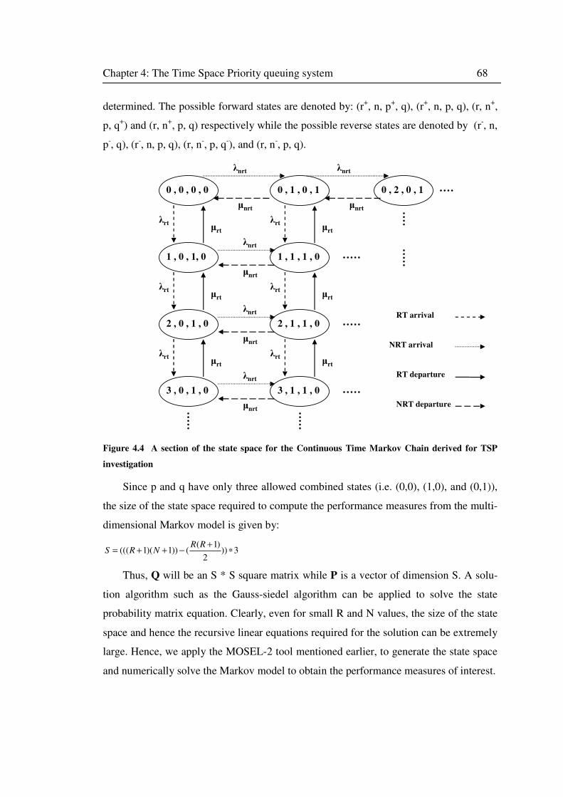
Chapter 4: The Time Space Priority queuing system 68
determined. The possible forward states are denoted by: (r+, n, p
+, q), (r
+, n, p, q), (r, n
+,
p, q+) and (r, n
+, p, q) respectively while the possible reverse states are denoted by (r
-, n,
p-, q), (r-, n, p, q), (r, n-, p, q-), and (r, n-, p, q).
NRT departure
λrt
λrt
λrtλrt
λrt
λrt
0 , 0 , 0 , 0 0 , 1 , 0 , 1
1 , 0 , 1, 0
2 , 0 , 1 , 0
3 , 0 , 1 , 0
1 , 1 , 1 , 0
2 , 1 , 1 , 0
3 , 1 , 1 , 0
0 , 2 , 0 , 1
µrt
µrt
µrt
µrt
µrt
µrt
λnrt
λnrt
λnrt
λnrt
λnrt
µnrt
µnrt
µnrt
µnrt µnrt
RT arrival
NRT arrival
RT departure
Figure 4.4 A section of the state space for the Continuous Time Markov Chain derived for TSP
investigation
Since p and q have only three allowed combined states (i.e. (0,0), (1,0), and (0,1)),
the size of the state space required to compute the performance measures from the multi-
dimensional Markov model is given by:
( 1)((( 1)( 1)) ( )) 3
2
R RS R N
+= + + − ∗
Thus, Q will be an S * S square matrix while P is a vector of dimension S. A solu-
tion algorithm such as the Gauss-siedel algorithm can be applied to solve the state
probability matrix equation. Clearly, even for small R and N values, the size of the state
space and hence the recursive linear equations required for the solution can be extremely
large. Hence, we apply the MOSEL-2 tool mentioned earlier, to generate the state space
and numerically solve the Markov model to obtain the performance measures of interest.
Chapter 4: The Time Space Priority queuing system 69
Let the following notations define the mathematical model parameters used in the
Markov model:
• λrt : mean RT packet arrival rate.
• λnrt : mean NRT packet arrival rate.
• µrt : mean RT packet service rate.
• µnrt: mean NRT packet service rate.
• R: Maximum number of admissible RT packets into the TSP queue.
• N: Maximum number of admissible packets (RT and NRT) into the TSP queue.
• p and q are HOL state indicators for the RT and NRT flows respectively.
The events, rules and rates for the possible transitions are:
• RT packet arrivals: An RT packet is admitted into the queue if the number of RT
packets is less than R i.e. r < R. If r < R and r + n = N (full buffer), then an NRT
packet is dropped from the queue tail to accommodate the arriving RT packet.
The first part of Table 4.1 shows the conditions, the successor states and the tran-
sition rates for this event.
• NRT packet arrivals: In accordance to the TSP buffer admission mechanism, an
NRT packet is admitted into the queue if the total number of RT and NRT packets
is less than N i.e. n + r < N. The bottom part of Table 4.1 shows the conditions, the
successor states and the transition rates for the NRT packet arrival event.
• RT packet transmission: Whenever the packet at the HOL is an RT packet, it is
transmitted on the common channel. It is assumed that only one packet can be
transmitted at a time. Thus while an RT packet is being transmitted p=1 and q=0,
as shown in the top half of Table 4.2.
• NRT packet transmission: NRT packets only get to the HOL of the (logical) queue
when no RT packets are present. This is indicated by p=0 and q=1. The bottom
half of Table 4.2 shows the rates, conditions and successor states for NRT trans-
mission event.
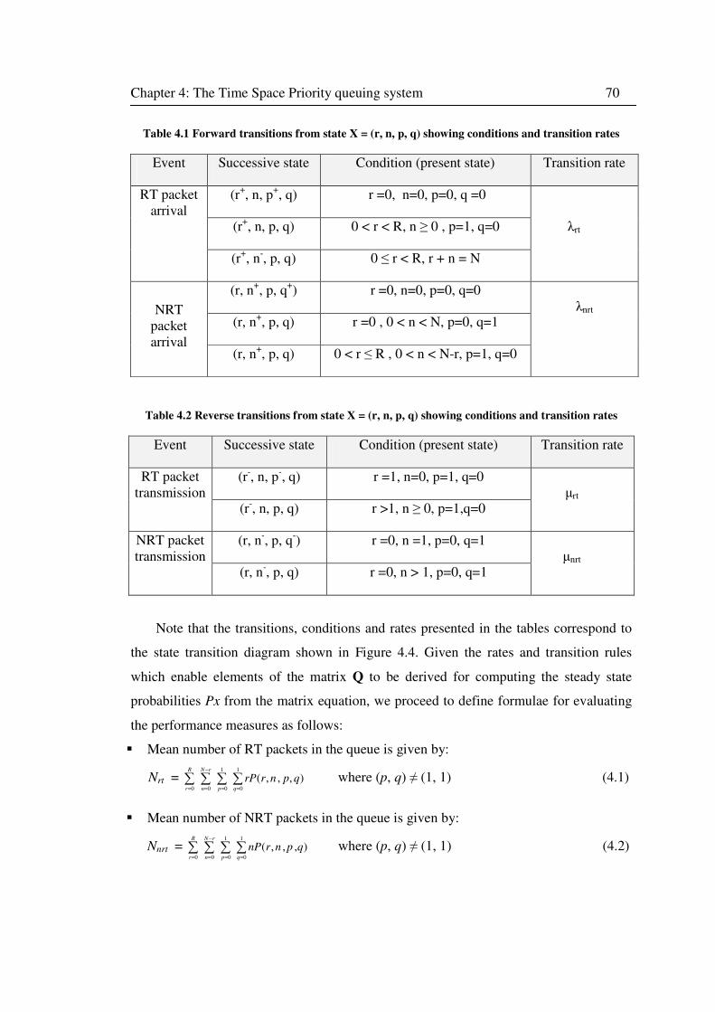
Chapter 4: The Time Space Priority queuing system 70
Table 4.1 Forward transitions from state X = (r, n, p, q) showing conditions and transition rates
Event Successive state Condition (present state) Transition rate
RT packet
arrival
(r+, n, p
+, q) r =0, n=0, p=0, q =0
λrt (r+, n, p, q) 0 < r < R, n ≥ 0 , p=1, q=0
(r+, n
-, p, q) 0 ≤ r < R, r + n = N
NRT
packet
arrival
(r, n+, p, q
+) r =0, n=0, p=0, q=0
λnrt
(r, n
+, p, q) r =0 , 0 < n < N, p=0, q=1
(r, n+, p, q) 0 < r ≤ R , 0 < n < N-r, p=1, q=0
Table 4.2 Reverse transitions from state X = (r, n, p, q) showing conditions and transition rates
Event Successive state Condition (present state) Transition rate
RT packet
transmission
(r-, n, p
-, q) r =1, n=0, p=1, q=0
µrt (r
-, n, p, q) r >1, n ≥ 0, p=1,q=0
NRT packet
transmission
(r, n-, p, q
-) r =0, n =1, p=0, q=1
µnrt (r, n
-, p, q) r =0, n > 1, p=0, q=1
Note that the transitions, conditions and rates presented in the tables correspond to
the state transition diagram shown in Figure 4.4. Given the rates and transition rules
which enable elements of the matrix Q to be derived for computing the steady state
probabilities Px from the matrix equation, we proceed to define formulae for evaluating
the performance measures as follows:
� Mean number of RT packets in the queue is given by:
Nrt = 1 1
0 0 0 0
( , , , )R N r
r n p q
rP r n p q−
= = = =
∑ ∑ ∑ ∑ where (p, q) ≠ (1, 1) (4.1)
� Mean number of NRT packets in the queue is given by:
Nnrt = 1 1
0 0 0 0
( , , , )R N r
r n p q
nP r n p q−
= = = =
∑ ∑ ∑ ∑ where (p, q) ≠ (1, 1) (4.2)
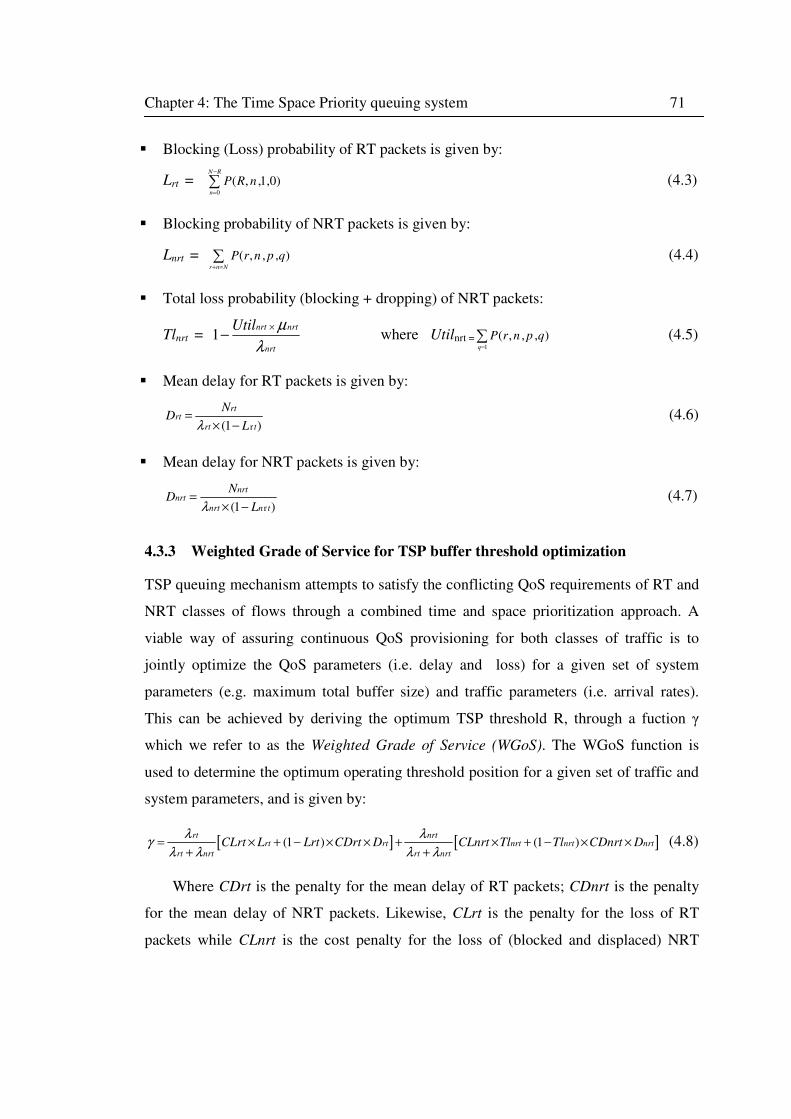
Chapter 4: The Time Space Priority queuing system 71
� Blocking (Loss) probability of RT packets is given by:
Lrt = 0
( , ,1,0)N R
n
P R n−
=
∑ (4.3)
� Blocking probability of NRT packets is given by:
Lnrt = ( , , , )r n N
P r n p q+ =
∑ (4.4)
� Total loss probability (blocking + dropping) of NRT packets:
Tlnrt = 1nrt nrt
nrt
Util µ
λ
×− where Utilnrt =
1
( , , , )q
P r n p q=
∑ (4.5)
� Mean delay for RT packets is given by:
r(1 )
rtrt
rt t
ND
Lλ=
× − (4.6)
� Mean delay for NRT packets is given by:
r(1 )
nrtnrt
nrt n t
ND
Lλ=
× − (4.7)
4.3.3 Weighted Grade of Service for TSP buffer threshold optimization
TSP queuing mechanism attempts to satisfy the conflicting QoS requirements of RT and
NRT classes of flows through a combined time and space prioritization approach. A
viable way of assuring continuous QoS provisioning for both classes of traffic is to
jointly optimize the QoS parameters (i.e. delay and loss) for a given set of system
parameters (e.g. maximum total buffer size) and traffic parameters (i.e. arrival rates).
This can be achieved by deriving the optimum TSP threshold R, through a fuction γ
which we refer to as the Weighted Grade of Service (WGoS). The WGoS function is
used to determine the optimum operating threshold position for a given set of traffic and
system parameters, and is given by:
[ ] [ ](1 ) (1 )rt nrt
rt rt nrt nrt nrt
rt nrt rt nrt
CLrt L Lrt CDrt D CLnrt Tl Tl CDnrt Dλ λ
γλ λ λ λ
= × + − × × + × + − × ×+ +
(4.8)
Where CDrt is the penalty for the mean delay of RT packets; CDnrt is the penalty
for the mean delay of NRT packets. Likewise, CLrt is the penalty for the loss of RT
packets while CLnrt is the cost penalty for the loss of (blocked and displaced) NRT
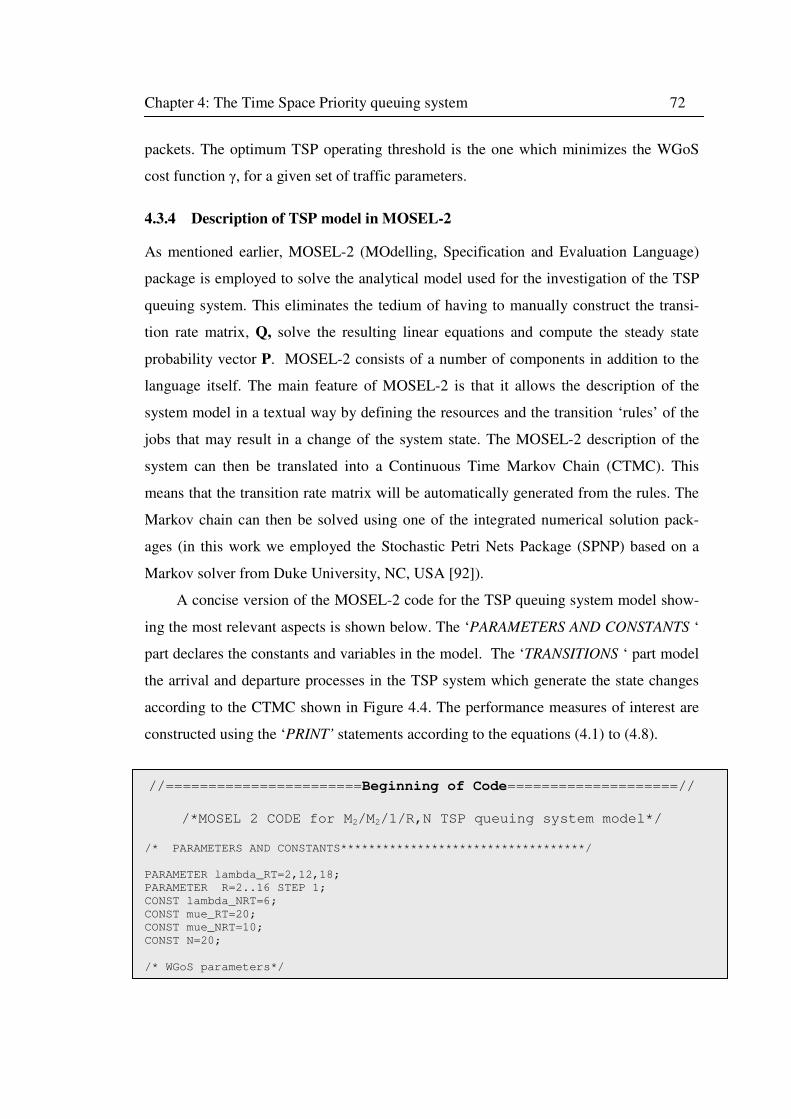
Chapter 4: The Time Space Priority queuing system 72
packets. The optimum TSP operating threshold is the one which minimizes the WGoS
cost function γ, for a given set of traffic parameters.
4.3.4 Description of TSP model in MOSEL-2
As mentioned earlier, MOSEL-2 (MOdelling, Specification and Evaluation Language)
package is employed to solve the analytical model used for the investigation of the TSP
queuing system. This eliminates the tedium of having to manually construct the transi-
tion rate matrix, Q, solve the resulting linear equations and compute the steady state
probability vector P. MOSEL-2 consists of a number of components in addition to the
language itself. The main feature of MOSEL-2 is that it allows the description of the
system model in a textual way by defining the resources and the transition ‘rules’ of the
jobs that may result in a change of the system state. The MOSEL-2 description of the
system can then be translated into a Continuous Time Markov Chain (CTMC). This
means that the transition rate matrix will be automatically generated from the rules. The
Markov chain can then be solved using one of the integrated numerical solution pack-
ages (in this work we employed the Stochastic Petri Nets Package (SPNP) based on a
Markov solver from Duke University, NC, USA [92]).
A concise version of the MOSEL-2 code for the TSP queuing system model show-
ing the most relevant aspects is shown below. The ‘PARAMETERS AND CONSTANTS ‘
part declares the constants and variables in the model. The ‘TRANSITIONS ‘ part model
the arrival and departure processes in the TSP system which generate the state changes
according to the CTMC shown in Figure 4.4. The performance measures of interest are
constructed using the ‘PRINT’ statements according to the equations (4.1) to (4.8).
//=======================Beginning of Code====================//
/*MOSEL 2 CODE for M2/M2/1/R,N TSP queuing system model*/
/* PARAMETERS AND CONSTANTS***********************************/
PARAMETER lambda_RT=2,12,18;
PARAMETER R=2..16 STEP 1;
CONST lambda_NRT=6;
CONST mue_RT=20;
CONST mue_NRT=10;
CONST N=20;
/* WGoS parameters*/
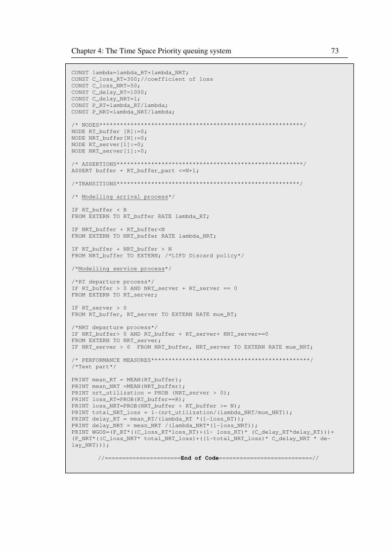
Chapter 4: The Time Space Priority queuing system 73
CONST lambda=lambda_RT+lambda_NRT;
CONST C_loss_RT=300;//coefficient of loss
CONST C_loss_NRT=50;
CONST C_delay_RT=1000;
CONST C_delay_NRT=1;
CONST P_RT=lambda_RT/lambda;
CONST P_NRT=lambda_NRT/lambda;
/* NODES***********************************************************/
NODE RT_buffer [R]:=0;
NODE NRT_buffer[N]:=0;
NODE RT_server[1]:=0;
NODE NRT_server[1]:=0;
/* ASSERTIONS******************************************************/
ASSERT buffer + RT_buffer_part <=N+1;
/*TRANSITIONS*****************************************************/
/* Modelling arrival process*/
IF RT_buffer < R
FROM EXTERN TO RT_buffer RATE lambda_RT;
IF NRT_buffer + RT_buffer<N
FROM EXTERN TO NRT_buffer RATE lambda_NRT;
IF RT_buffer + NRT_buffer > N
FROM NRT_buffer TO EXTERN; /*LIFD Discard policy*/
/*Modelling service process*/
/*RT departure process*/
IF RT_buffer > 0 AND NRT_server + RT_server == 0
FROM EXTERN TO RT_server;
IF RT_server > 0
FROM RT_buffer, RT_server TO EXTERN RATE mue_RT;
/*NRT departure process*/
IF NRT_buffer> 0 AND RT_buffer + RT_server+ NRT_server==0
FROM EXTERN TO NRT_server;
IF NRT_server > 0 FROM NRT_buffer, NRT_server TO EXTERN RATE mue_NRT;
/* PERFORMANCE MEASURES**********************************************/
/*Text part*/
PRINT mean_RT = MEAN(RT_buffer);
PRINT mean_NRT =MEAN(NRT_buffer);
PRINT nrt_utilization = PROB (NRT_server > 0);
PRINT loss_RT=PROB(RT_buffer==R);
PRINT loss_NRT=PROB(NRT_buffer + RT_buffer >= N);
PRINT total_NRT_loss = 1-(nrt_utilization/(lambda_NRT/mue_NRT));
PRINT delay_RT = mean_RT/(lambda_RT *(1-loss_RT));
PRINT delay_NRT = mean_NRT /(lambda_NRT*(1-loss_NRT));
PRINT WGOS=(P_RT*((C_loss_RT*loss_RT)+(1- loss_RT)* (C_delay_RT*delay_RT)))+
(P_NRT*((C_loss_NRT* total_NRT_loss)+((1-total_NRT_loss)* C_delay_NRT * de-
lay_NRT)));
//======================End of Code===========================//
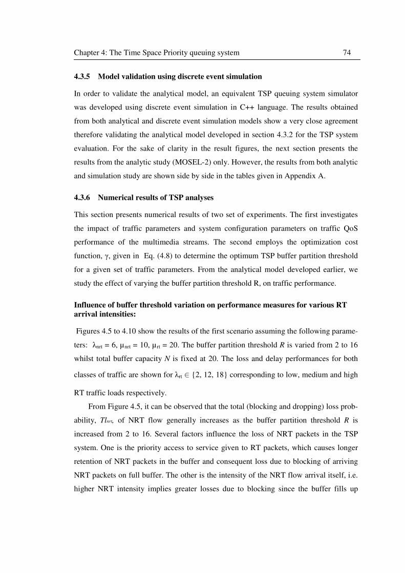
Chapter 4: The Time Space Priority queuing system 74
4.3.5 Model validation using discrete event simulation
In order to validate the analytical model, an equivalent TSP queuing system simulator
was developed using discrete event simulation in C++ language. The results obtained
from both analytical and discrete event simulation models show a very close agreement
therefore validating the analytical model developed in section 4.3.2 for the TSP system
evaluation. For the sake of clarity in the result figures, the next section presents the
results from the analytic study (MOSEL-2) only. However, the results from both analytic
and simulation study are shown side by side in the tables given in Appendix A.
4.3.6 Numerical results of TSP analyses
This section presents numerical results of two set of experiments. The first investigates
the impact of traffic parameters and system configuration parameters on traffic QoS
performance of the multimedia streams. The second employs the optimization cost
function, γ, given in Eq. (4.8) to determine the optimum TSP buffer partition threshold
for a given set of traffic parameters. From the analytical model developed earlier, we
study the effect of varying the buffer partition threshold R, on traffic performance.
Influence of buffer threshold variation on performance measures for various RT
arrival intensities:
Figures 4.5 to 4.10 show the results of the first scenario assuming the following parame-
ters: λnrt = 6, µnrt = 10, µ rt = 20. The buffer partition threshold R is varied from 2 to 16
whilst total buffer capacity N is fixed at 20. The loss and delay performances for both
classes of traffic are shown for λrt ∈ {2, 12, 18} corresponding to low, medium and high
RT traffic loads respectively.
From Figure 4.5, it can be observed that the total (blocking and dropping) loss prob-
ability, Tlnrt, of NRT flow generally increases as the buffer partition threshold R is
increased from 2 to 16. Several factors influence the loss of NRT packets in the TSP
system. One is the priority access to service given to RT packets, which causes longer
retention of NRT packets in the buffer and consequent loss due to blocking of arriving
NRT packets on full buffer. The other is the intensity of the NRT flow arrival itself, i.e.
higher NRT intensity implies greater losses due to blocking since the buffer fills up
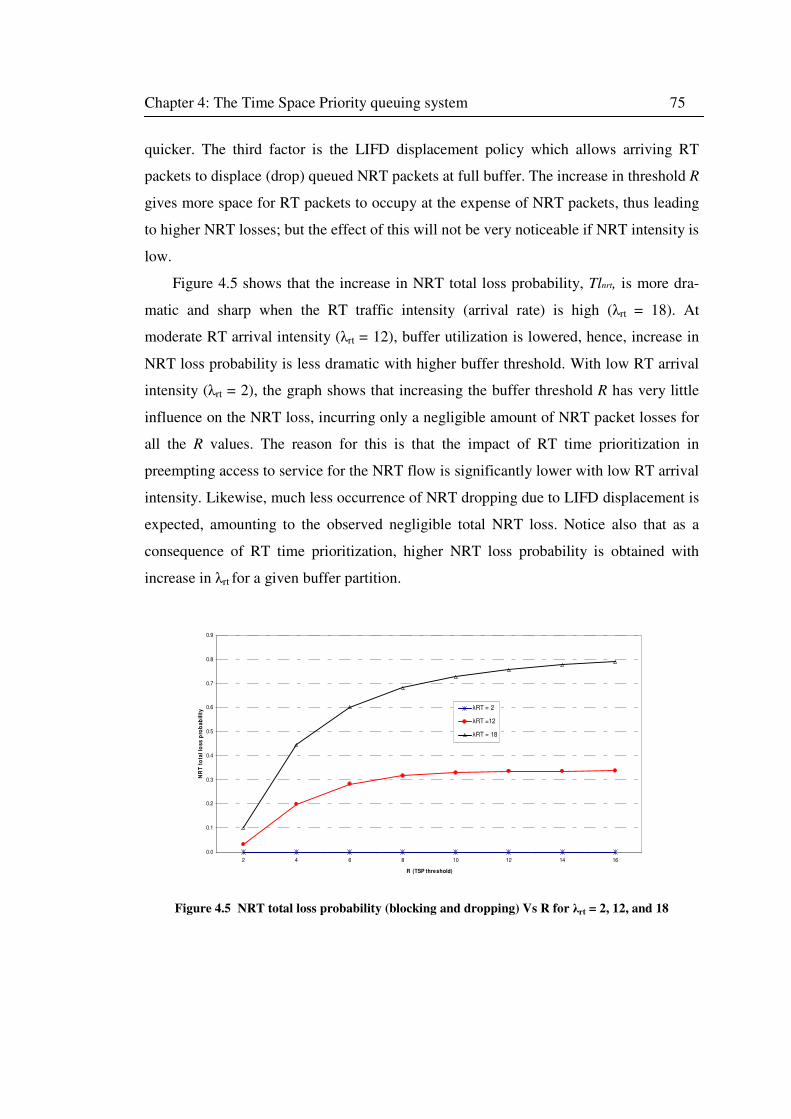
Chapter 4: The Time Space Priority queuing system 75
quicker. The third factor is the LIFD displacement policy which allows arriving RT
packets to displace (drop) queued NRT packets at full buffer. The increase in threshold R
gives more space for RT packets to occupy at the expense of NRT packets, thus leading
to higher NRT losses; but the effect of this will not be very noticeable if NRT intensity is
low.
Figure 4.5 shows that the increase in NRT total loss probability, Tlnrt, is more dra-
matic and sharp when the RT traffic intensity (arrival rate) is high (λrt = 18). At
moderate RT arrival intensity (λrt = 12), buffer utilization is lowered, hence, increase in
NRT loss probability is less dramatic with higher buffer threshold. With low RT arrival
intensity (λrt = 2), the graph shows that increasing the buffer threshold R has very little
influence on the NRT loss, incurring only a negligible amount of NRT packet losses for
all the R values. The reason for this is that the impact of RT time prioritization in
preempting access to service for the NRT flow is significantly lower with low RT arrival
intensity. Likewise, much less occurrence of NRT dropping due to LIFD displacement is
expected, amounting to the observed negligible total NRT loss. Notice also that as a
consequence of RT time prioritization, higher NRT loss probability is obtained with
increase in λrt for a given buffer partition.
0.0
0.1
0.2
0.3
0.4
0.5
0.6
0.7
0.8
0.9
2 4 6 8 10 12 14 16
R (TSP threshold)
NR
T t
ota
l lo
ss
pro
ba
bil
ity λRT = 2
λRT =12
λRT = 18
Figure 4.5 NRT total loss probability (blocking and dropping) Vs R for λrt = 2, 12, and 18
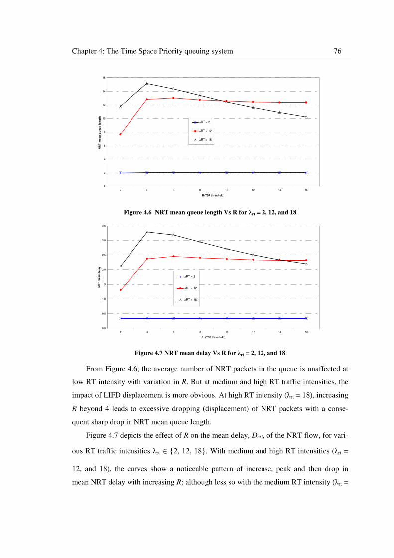
Chapter 4: The Time Space Priority queuing system 76
0
2
4
6
8
10
12
14
16
2 4 6 8 10 12 14 16
R (TSP threshold)
NR
T m
ea
n q
ue
ue
le
ng
th
λRT = 2
λRT = 12
λRT = 18
Figure 4.6 NRT mean queue length Vs R for λrt = 2, 12, and 18
0.0
0.5
1.0
1.5
2.0
2.5
3.0
3.5
2 4 6 8 10 12 14 16
R (TSP threshold)
NR
T m
ea
n d
ela
y
λRT = 2
λRT = 12
λRT = 18
Figure 4.7 NRT mean delay Vs R for λrt = 2, 12, and 18
From Figure 4.6, the average number of NRT packets in the queue is unaffected at
low RT intensity with variation in R. But at medium and high RT traffic intensities, the
impact of LIFD displacement is more obvious. At high RT intensity (λrt = 18), increasing
R beyond 4 leads to excessive dropping (displacement) of NRT packets with a conse-
quent sharp drop in NRT mean queue length.
Figure 4.7 depicts the effect of R on the mean delay, Dnrt, of the NRT flow, for vari-
ous RT traffic intensities λrt ∈ {2, 12, 18}. With medium and high RT intensities (λrt =
12, and 18), the curves show a noticeable pattern of increase, peak and then drop in
mean NRT delay with increasing R; although less so with the medium RT intensity (λrt =
Chapter 4: The Time Space Priority queuing system 77
12). Since more RT traffic is retained as buffer threshold R is increased, the effect of
priority access to service has a larger influence in delaying the access to service for NRT
flow; which explains the initial rise in NRT mean delay with higher R. On the other
hand, more NRT packets are likely be lost due to LIFD displacement as R is increased.
Thus, beyond the peak delay, the drop corresponds to less retention of NRT packets in
the buffer as a result of LIFD displacement. Consequently, a lower mean delay is
experienced by the (retained) NRT packets that eventually get access to service. Also, as
with the NRT total loss, mean delay for NRT flow also increases with increase in RT
traffic intensity, λrt.
Figure 4.8 shows the influence of R on the RT loss probability, Lrt, of the RT flow,
for various RT traffic intensities λrt ∈ {2, 12, 18}. As expected, RT loss probability
decreases when R is increased. Similarly, RT loss probability drops as the intensity of
RT arrival is decreased.
Figure 4.10 presents the results of mean RT delay, Drt, for different RT intensities λrt
∈ {2, 12, 18} as R is varied from 2 to 16. Mean RT delay is seen to increase with R for
medium (λrt = 12) and high (λrt = 18) traffic intensities, but more dramatically rising for
the high RT arrival intensity. At low RT arrival rate (λrt = 2), mean RT delay is hardly
influenced by the threshold value R, because of the combined effect of high RT service
rate (compared to the RT arrival rate) and priority access to service. The curves in Figure
4.9 showing the average number of RT packets in the queue depict a similar pattern to
the corresponding RT delay curves (in Figure 4.10) as expected from equation (4.6).
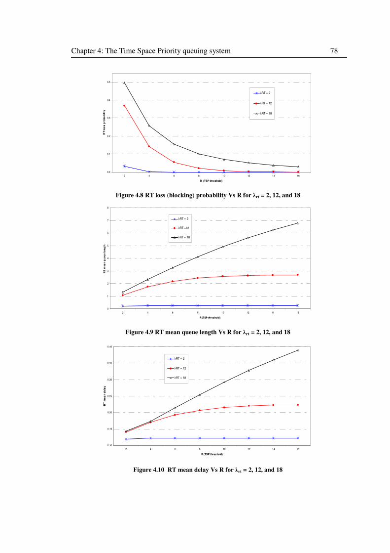
Chapter 4: The Time Space Priority queuing system 78
0.0
0.1
0.2
0.3
0.4
0.5
2 4 6 8 10 12 14 16
R (TSP threshold)
RT
los
s p
rob
ab
ilit
y
λRT = 2
λRT = 12
λRT = 18
Figure 4.8 RT loss (blocking) probability Vs R for λrt = 2, 12, and 18
0
1
2
3
4
5
6
7
8
2 4 6 8 10 12 14 16
R (TSP threshold)
RT
me
an
qu
eu
e l
en
gth
λRT = 2
λRT =12
λRT = 18
Figure 4.9 RT mean queue length Vs R for λrt = 2, 12, and 18
0.10
0.15
0.20
0.25
0.30
0.35
0.40
2 4 6 8 10 12 14 16
R (TSP threshold)
RT
me
an
de
lay
λRT = 2
λRT = 12
λRT = 18
Figure 4.10 RT mean delay Vs R for λrt = 2, 12, and 18
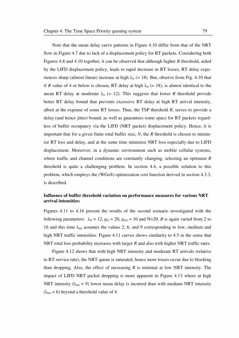
Chapter 4: The Time Space Priority queuing system 79
Note that the mean delay curve patterns in Figure 4.10 differ from that of the NRT
flow in Figure 4.7 due to lack of a displacement policy for RT packets. Considering both
Figures 4.8 and 4.10 together, it can be observed that although higher R threshold, aided
by the LIFD displacement policy, leads to rapid decrease in RT losses, RT delay expe-
riences sharp (almost linear) increase at high λrt (= 18). But, observe from Fig. 4.10 that
if R value of 4 or below is chosen, RT delay at high λrt (= 18), is almost identical to the
mean RT delay at moderate λrt (= 12). This suggests that lower R threshold provide
better RT delay bound that prevents excessive RT delay at high RT arrival intensity,
albeit at the expense of some RT losses. Thus, the TSP threshold R, serves to provide a
delay (and hence jitter) bound, as well as guarantees some space for RT packets regard-
less of buffer occupancy via the LIFD (NRT packet) displacement policy. Hence, it is
important that for a given finite total buffer size, N, the R threshold is chosen to minim-
ize RT loss and delay, and at the same time minimize NRT loss especially due to LIFD
displacement. Moreover, in a dynamic environment such as mobile cellular systems,
where traffic and channel conditions are constantly changing, selecting an optimum R
threshold is quite a challenging problem. In section 4.4, a possible solution to this
problem, which employs the (WGoS) optimization cost function derived in section 4.3.3,
is described.
Influence of buffer threshold variation on performance measures for various NRT
arrival intensities:
Figures 4.11 to 4.16 present the results of the second scenario investigated with the
following parameters: λrt = 12, µ rt = 20, µnrt = 10 and N=20. R is again varied from 2 to
16 and this time λnrt assumes the values 2, 6, and 9 corresponding to low, medium and
high NRT traffic intensities. Figure 4.11 curves shows similarity to 4.5 in the sense that
NRT total loss probability increases with larger R and also with higher NRT traffic rates.
Figure 4.12 shows that with high NRT intensity and moderate RT arrivals (relative
to RT service rate), the NRT queue is saturated, hence more losses occur due to blocking
than dropping. Also, the effect of increasing R is minimal at low NRT intensity. The
impact of LIFD NRT packet dropping is more apparent in Figure 4.13 where at high
NRT intensity (λnrt = 9) lower mean delay is incurred than with medium NRT intensity
(λnrt = 6) beyond a threshold value of 4.
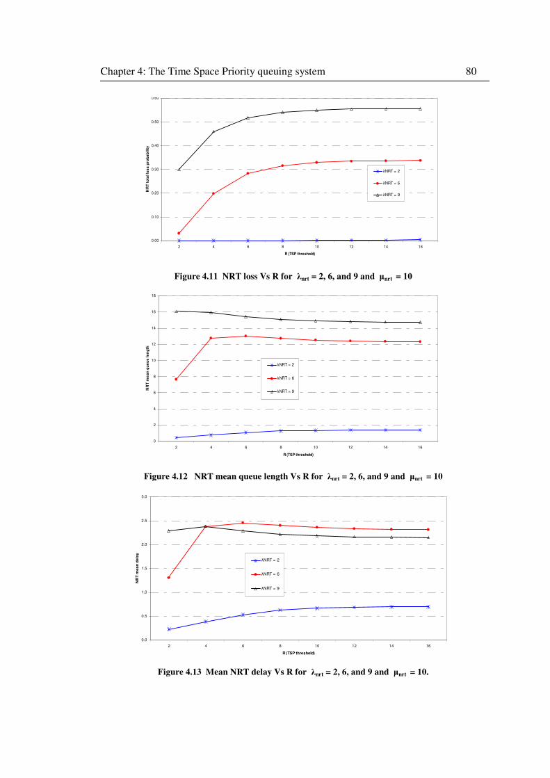
Chapter 4: The Time Space Priority queuing system 80
0.00
0.10
0.20
0.30
0.40
0.50
0.60
2 4 6 8 10 12 14 16
R (TSP threshold)
NR
T t
ota
l lo
ss
pro
ba
bilit
y
λNRT = 2
λNRT = 6
λNRT = 9
Figure 4.11 NRT loss Vs R for λnrt = 2, 6, and 9 and µnrt = 10
0
2
4
6
8
10
12
14
16
18
2 4 6 8 10 12 14 16
R (TSP threshold)
NR
T m
ea
n q
ue
ue
le
ng
th
λNRT = 2
λNRT = 6
λNRT = 9
Figure 4.12 NRT mean queue length Vs R for λnrt = 2, 6, and 9 and µnrt = 10
0.0
0.5
1.0
1.5
2.0
2.5
3.0
2 4 6 8 10 12 14 16
R (TSP threshold)
NR
T m
ea
n d
ela
y
λNRT = 2
λNRT = 6
λNRT = 9
Figure 4.13 Mean NRT delay Vs R for λnrt = 2, 6, and 9 and µnrt = 10.
Chapter 4: The Time Space Priority queuing system 81
Finally, the RT traffic performance curves for the second scenario are depicted in
Figures 4.14 to 4.16. RT loss probability is seen to decrease with R as expected (c.f.
Figure 4.14), but, increasing NRT intensity from medium to high loads seem to have
very little effect on RT loss. This could also be attributed to the prioritized access to
service accorded to RT traffic and also the LIFD displacement policy, which to some
extent shields RT performance from the effects of λnrt variation. From Figures 4.15 and
4.16 we also see that as R increases so does mean RT queue length and mean RT delay
respectively, while again showing a similar pattern as expected from equation (4.6).
Again, due to RT service priority access and LIFD displacement, an increase in NRT
traffic intensity from moderate to high rates (λnrt = 6 to λnrt = 9) have only marginal
effect on the mean RT queue occupancy and hence the mean delay.
The results of the experiments suggest that varying the buffer TSP partition thre-
shold affect the QoS performance metrics of the multimedia traffic differently. Thus, an
optimum threshold can be found by trading off one QoS performance metric against its
conflicting counterpart. The WGoS function γ, presented in section 4.3.3 provides an
effective method using the RT and NRT flows’ QoS performance trade-offs in finding
the optimum threshold.
0.00
0.05
0.10
0.15
0.20
0.25
0.30
0.35
0.40
2 4 6 8 10 12 14 16
R (TSP threshold)
RT
lo
ss
pro
ba
bilit
y
λNRT = 2
λNRT = 6
λNRT = 9
Figure 4.14 RT loss Vs R for λnrt = 2, 6, and 9 and µnrt = 10
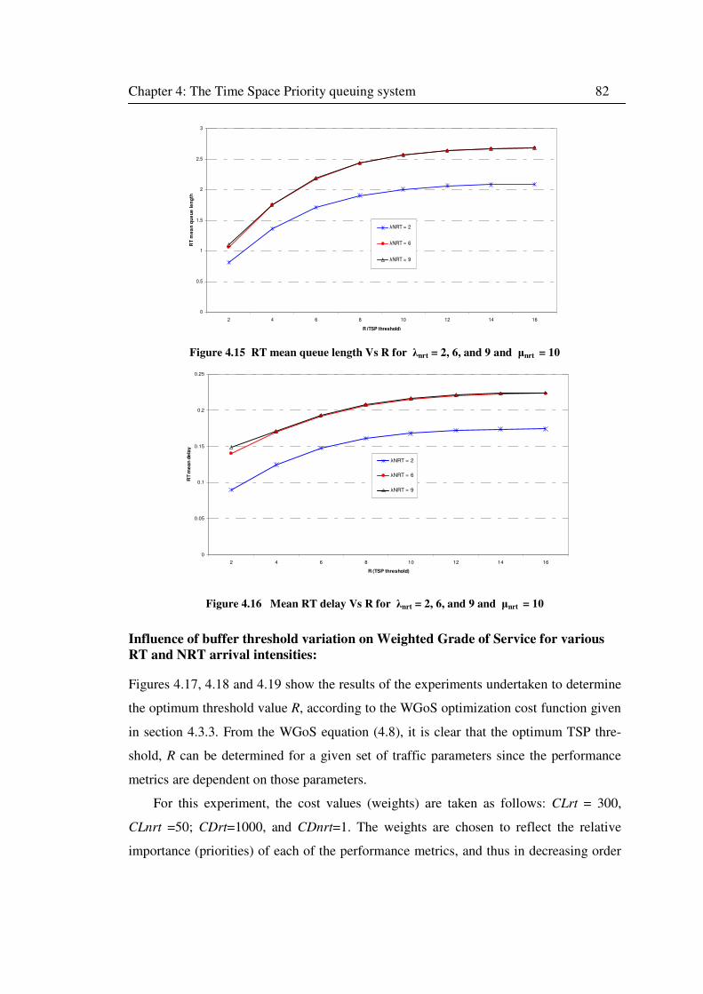
Chapter 4: The Time Space Priority queuing system 82
0
0.5
1
1.5
2
2.5
3
2 4 6 8 10 12 14 16
R (TSP threshold)
RT
me
an
qu
eu
e le
ng
th
λNRT = 2
λNRT = 6
λNRT = 9
Figure 4.15 RT mean queue length Vs R for λnrt = 2, 6, and 9 and µnrt = 10
0
0.05
0.1
0.15
0.2
0.25
2 4 6 8 10 12 14 16
R (TSP threshold)
RT
me
an
de
lay
λNRT = 2
λNRT = 6
λNRT = 9
Figure 4.16 Mean RT delay Vs R for λnrt = 2, 6, and 9 and µnrt = 10
Influence of buffer threshold variation on Weighted Grade of Service for various
RT and NRT arrival intensities:
Figures 4.17, 4.18 and 4.19 show the results of the experiments undertaken to determine
the optimum threshold value R, according to the WGoS optimization cost function given
in section 4.3.3. From the WGoS equation (4.8), it is clear that the optimum TSP thre-
shold, R can be determined for a given set of traffic parameters since the performance
metrics are dependent on those parameters.
For this experiment, the cost values (weights) are taken as follows: CLrt = 300,
CLnrt =50; CDrt=1000, and CDnrt=1. The weights are chosen to reflect the relative
importance (priorities) of each of the performance metrics, and thus in decreasing order
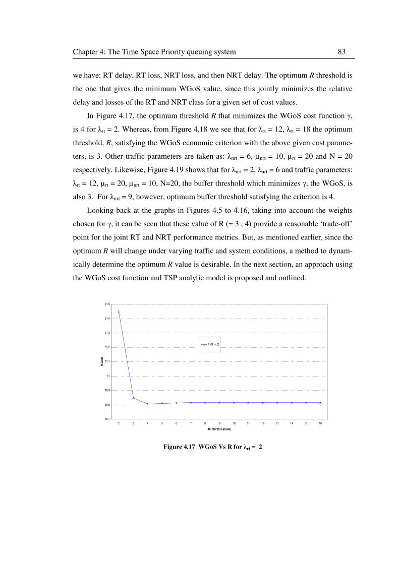
Chapter 4: The Time Space Priority queuing system 83
we have: RT delay, RT loss, NRT loss, and then NRT delay. The optimum R threshold is
the one that gives the minimum WGoS value, since this jointly minimizes the relative
delay and losses of the RT and NRT class for a given set of cost values.
In Figure 4.17, the optimum threshold R that minimizes the WGoS cost function γ,
is 4 for λrt = 2. Whereas, from Figure 4.18 we see that for λrt = 12, λrt = 18 the optimum
threshold, R, satisfying the WGoS economic criterion with the above given cost parame-
ters, is 3. Other traffic parameters are taken as: λnrt = 6, µnrt = 10, µ rt = 20 and N = 20
respectively. Likewise, Figure 4.19 shows that for λnrt = 2, λnrt = 6 and traffic parameters:
λrt = 12, µrt = 20, µnrt = 10, N=20, the buffer threshold which minimizes γ, the WGoS, is
also 3. For λnrt = 9, however, optimum buffer threshold satisfying the criterion is 4.
Looking back at the graphs in Figures 4.5 to 4.16, taking into account the weights
chosen for γ, it can be seen that these value of R (= 3 , 4) provide a reasonable ‘trade-off’
point for the joint RT and NRT performance metrics. But, as mentioned earlier, since the
optimum R will change under varying traffic and system conditions, a method to dynam-
ically determine the optimum R value is desirable. In the next section, an approach using
the WGoS cost function and TSP analytic model is proposed and outlined.
30.7
30.8
30.9
31
31.1
31.2
31.3
31.4
31.5
2 3 4 5 6 7 8 9 10 11 12 13 14 15 16
R (TSP threshold)
WG
oS
λRT = 2
Figure 4.17 WGoS Vs R for λrt = 2
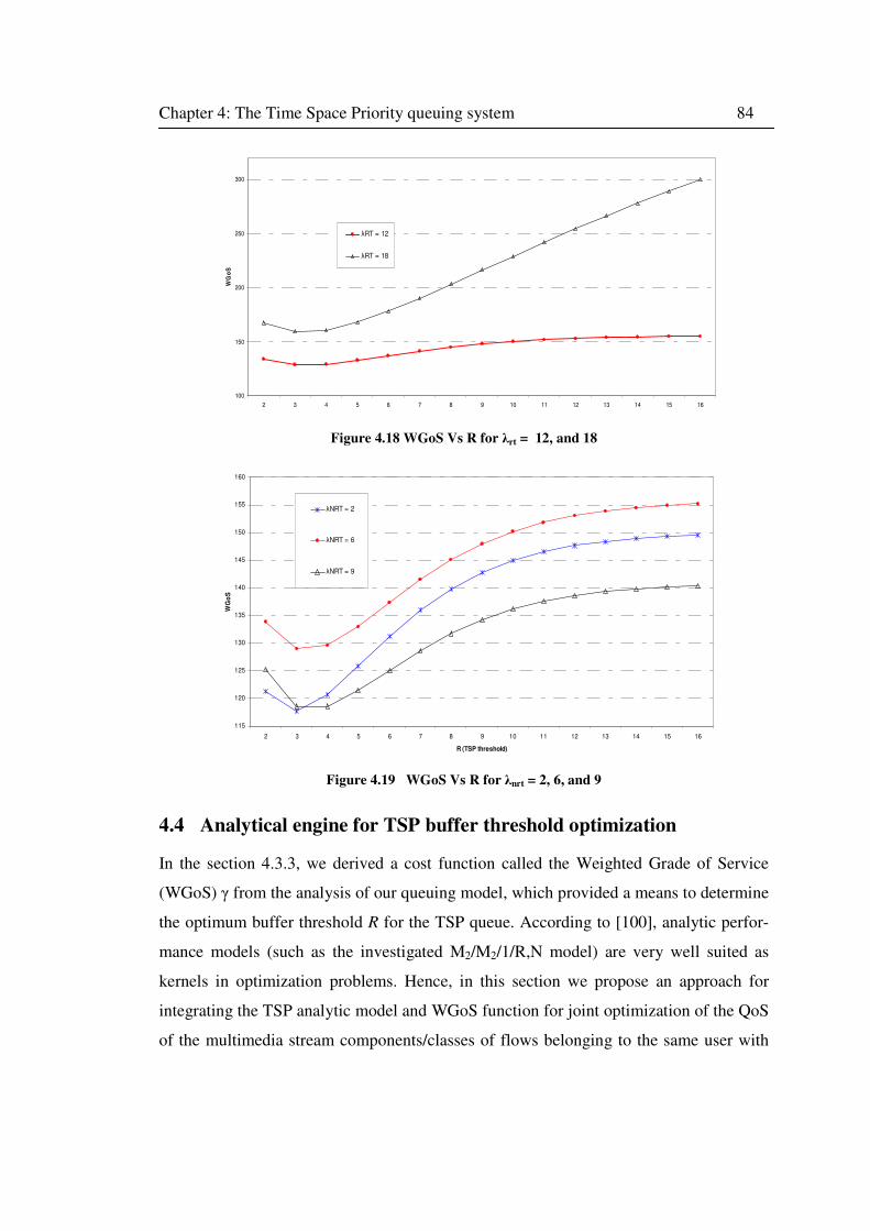
Chapter 4: The Time Space Priority queuing system 84
100
150
200
250
300
2 3 4 5 6 7 8 9 10 11 12 13 14 15 16
WG
oS
λRT = 12
λRT = 18
Figure 4.18 WGoS Vs R for λrt = 12, and 18
115
120
125
130
135
140
145
150
155
160
2 3 4 5 6 7 8 9 10 11 12 13 14 15 16
R (TSP threshold)
WG
oS
λNRT = 2
λNRT = 6
λNRT = 9
Figure 4.19 WGoS Vs R for λnrt = 2, 6, and 9
4.4 Analytical engine for TSP buffer threshold optimization
In the section 4.3.3, we derived a cost function called the Weighted Grade of Service
(WGoS) γ from the analysis of our queuing model, which provided a means to determine
the optimum buffer threshold R for the TSP queue. According to [100], analytic perfor-
mance models (such as the investigated M2/M2/1/R,N model) are very well suited as
kernels in optimization problems. Hence, in this section we propose an approach for
integrating the TSP analytic model and WGoS function for joint optimization of the QoS
of the multimedia stream components/classes of flows belonging to the same user with
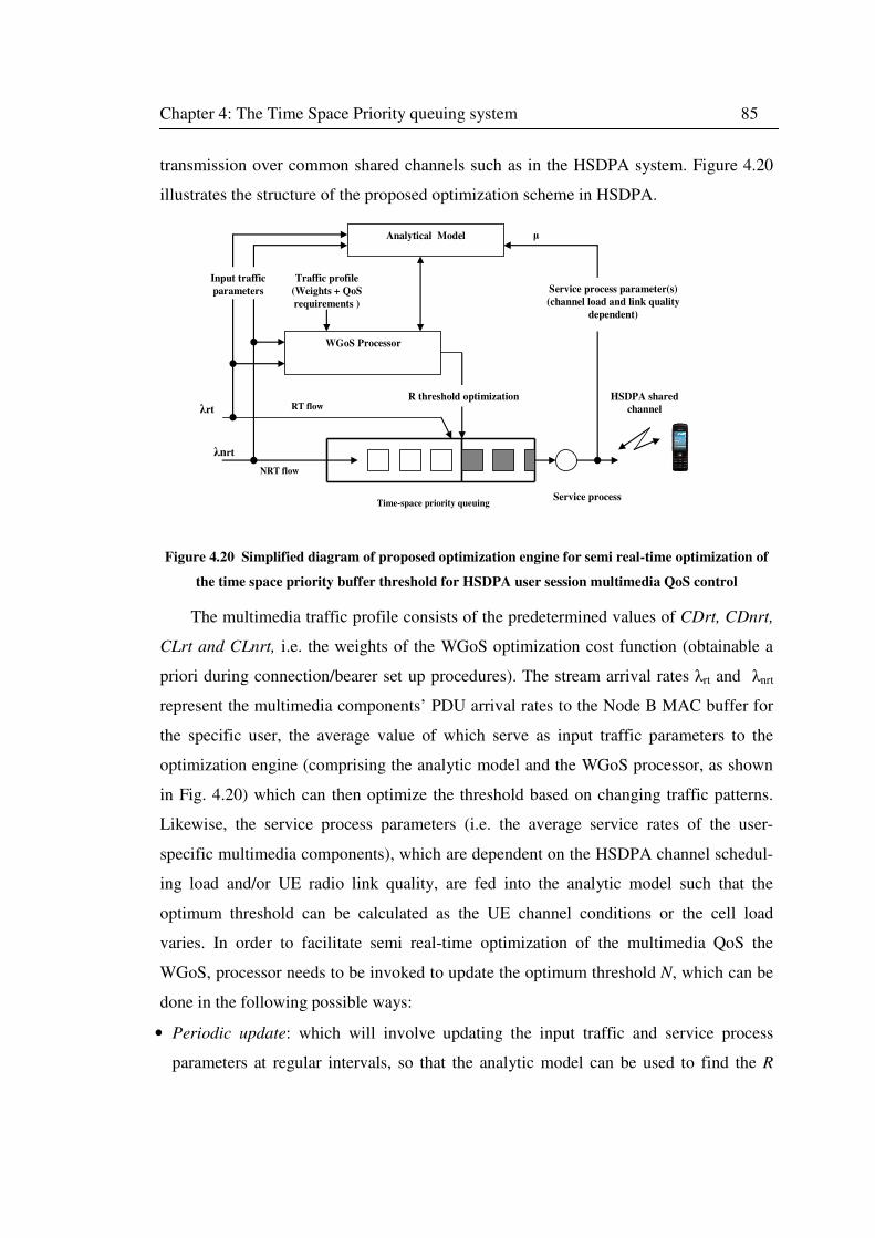
Chapter 4: The Time Space Priority queuing system 85
transmission over common shared channels such as in the HSDPA system. Figure 4.20
illustrates the structure of the proposed optimization scheme in HSDPA.
HSDPA shared
channel
NRT flow
λnrt
λrt
µ
RT flow
Analytical Model
WGoS Processor
Service process
R threshold optimization
Time-space priority queuing
Traffic profile
(Weights + QoS
requirements )
Input traffic
parameters Service process parameter(s)
(channel load and link quality
dependent)
Figure 4.20 Simplified diagram of proposed optimization engine for semi real-time optimization of
the time space priority buffer threshold for HSDPA user session multimedia QoS control
The multimedia traffic profile consists of the predetermined values of CDrt, CDnrt,
CLrt and CLnrt, i.e. the weights of the WGoS optimization cost function (obtainable a
priori during connection/bearer set up procedures). The stream arrival rates λrt and λnrt
represent the multimedia components’ PDU arrival rates to the Node B MAC buffer for
the specific user, the average value of which serve as input traffic parameters to the
optimization engine (comprising the analytic model and the WGoS processor, as shown
in Fig. 4.20) which can then optimize the threshold based on changing traffic patterns.
Likewise, the service process parameters (i.e. the average service rates of the user-
specific multimedia components), which are dependent on the HSDPA channel schedul-
ing load and/or UE radio link quality, are fed into the analytic model such that the
optimum threshold can be calculated as the UE channel conditions or the cell load
varies. In order to facilitate semi real-time optimization of the multimedia QoS the
WGoS, processor needs to be invoked to update the optimum threshold N, which can be
done in the following possible ways:
• Periodic update: which will involve updating the input traffic and service process
parameters at regular intervals, so that the analytic model can be used to find the R
Chapter 4: The Time Space Priority queuing system 86
value that minimizes the WGoS criterion, which will then be used as the threshold
value in the time space priority buffer management algorithm until the next update.
• Performance driven update: Given that an initial value for R is determined using the
QoS requirements given in the traffic profile, the system is then invoked to update the
threshold R whenever a given QoS performance measure (loss or delay) exceeds a
given allowable value. For example if Voice packet loss rate exceed 1% or the delay
exceeds a stated maximum value, then a threshold update can be triggered.
• Traffic triggered update: Changes in the traffic arrival pattern can also be used to
invoke the system to calculate a new optimum value R for the buffer optimization. For
example, when variation in arrival rates λrt and λnrt, to the base station is detected, a
new optimum value for R can be recalculated.
4.5 TSP vs. conventional priority queuing schemes
In this section, existing traditional queue management schemes commonly encountered
in the literature are used as reference for comparative analysis to the TSP queue man-
agement. This investigation is designed to give further insight into the merits and
constraints of TSP and to assess its capability to enable joint RT and NRT QoS control
compared to conventional queuing disciplines.
From the literature survey presented in chapter 2, we saw that most existing priority
queuing can be classed into complete buffer sharing (CBS), partial buffer sharing (PBS),
or complete buffer partitioning (CPB), from buffer resource management viewpoint;
while in terms of service differentiation strategy priority queuing can be based on time
priorities or space priorities.
Recall that the CBS queuing discipline ensures the highest possible overall buffer
utilization when applied to multiple-class traffic. Hence, CBS provides a baseline to
assess the buffer utilization properties of TSP. PBS, on the other hand, is the most
widely studied space priority scheme and provides a good baseline space priority
scheme for comparative study. CBP is well known for its fairness properties (in buffer
space allocation) especially under unbalanced/asymmetric traffic conditions. CBP
queuing is considered in the study, with Precedence Queuing (PQ) time prioritization
which always gives service priority to RT traffic over NRT traffic when both types are
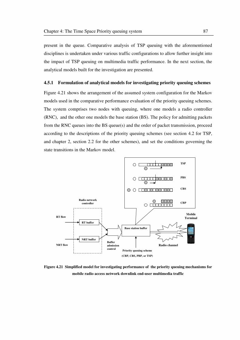
Chapter 4: The Time Space Priority queuing system 87
present in the queue. Comparative analysis of TSP queuing with the aforementioned
disciplines is undertaken under various traffic configurations to allow further insight into
the impact of TSP queuing on multimedia traffic performance. In the next section, the
analytical models built for the investigation are presented.
4.5.1 Formulation of analytical models for investigating priority queuing schemes
Figure 4.21 shows the arrangement of the assumed system configuration for the Markov
models used in the comparative performance evaluation of the priority queuing schemes.
The system comprises two nodes with queuing, where one models a radio controller
(RNC), and the other one models the base station (BS). The policy for admitting packets
from the RNC queues into the BS queue(s) and the order of packet transmission, proceed
according to the descriptions of the priority queuing schemes (see section 4.2 for TSP,
and chapter 2, section 2.2 for the other schemes), and set the conditions governing the
state transitions in the Markov model.
Buffer
admission
control
Mobile
Terminal
Base station buffer
Radio channel
Priority queuing scheme
(CBP, CBS, PBP, or TSP)
NRT buffer
RT flow
RT buffer
NRT flow
Radio network
controller
TSP
CBS
PBS
CBP
Figure 4.21 Simplified model for investigating performance of the priority queuing mechanisms for
mobile radio access network downlink end-user multimedia traffic
Chapter 4: The Time Space Priority queuing system 88
4.5.2 Basic system assumptions and notations
• Two classes of traffic, RT and NRT exist within a connection or session with ar-
rival to separate RNC queues according to independent Poisson process with
arrival rates λrt and λnrt respectively. The RNC queues are of limited capacity
hence arriving packets that encounter a full queue are discarded (as shown in Fig-
ure 4.21).
• We assume that packets are transmitted between the RNC and BS buffers without
any transmission loss or delay and proceed only when BS buffer admission control
policy -which differs with applied BS queuing scheme- permits.
• Let the radio link state ch assume either a ‘good’ state or ‘bad’ state corresponding
to favourable and unfavourable channel conditions respectively. Assuming the
time spent in each state is exponentially distributed, ch transits from ‘good’ to
‘bad’ (ch = 1 to ch =0 ) at an average rate of 1/(1- Pg) and from ‘bad’ to ‘good’ (ch
= 0 to ch =1 ) on average at the rate of 1/(1-Pb) = 1/Pg. Where Pg denotes probabili-
ty that ch is in ‘good’ state and Pb = 1-Pg denotes the probability of ch remaining
in ‘bad’ state. State ch, allows modelling an error-prone radio channel in the Mar-
kov chain to capture the effect of packet loss and retransmission on the air
interface due to unfavourable radio channel conditions. Thus, packet transmission
proceeds on the radio link, only when the channel state ch is ‘good’.
• Packet transmission times at the radio interface are assumed to be independent and
exponentially distributed with mean 1/µ, with the order of packet transmission de-
pending on the applied BS queuing scheme.
• Let R represent the total RNC RT queue capacity while N represents the total
RNC NRT queue capacity. Let r be the number of RT packets in the RNC RT
queue, and n the number of NRT packets in the NRT RNC queue at any given
time.
• Let T represent the total BS queue capacity. Also denote t = rb + nb as the total
number of packets present in the base station at any given time, where rb and nb
are the number of RT and NRT packets present respectively.
• Denote Rb as the TSP threshold in the BS queue i.e. maximum number of allowa-
ble RT packets according to TSP policy. Thus, with TSP queuing, RT packets are
Chapter 4: The Time Space Priority queuing system 89
moved from RNC RT queue to BS only when rb < Rb, while NRT packets move
from RNC NRT queue to BS whenever t < T.
• Denote Rc as the CBP partition which divides the BS queue such that the maxi-
mum allowable number of RT packets in the BS queue is given by Rc for CBP.
• Let th denote the PBS threshold in the BS queue, when PBS queuing is applied.
• Finally, denote by p = 1 the state when the head-of-the-line BS queue packet wait-
ing for transmission is an RT packet and p = 0 otherwise; and by q = 1, when the
head-of-the-line packet awaiting transmission is an NRT packet and q = 0 other-
wise. Empty state of the BS queue is given by p = 0, q = 0.
4.5.3 The Markov models
Let the state of the system be defined by a vector X = J’ where J’ = ( r, n, t, p, q, ch)
when TSP or CBP is applied in the BS queue, and J’ = ( r, n, t, ch) when either PBS or
CBS policy is applied in the BS queue. Let the number of possible states in the Markov
chain be given by M. We can thus define K to represent the finite state space of the
system(s) given that the states are conveniently ordered from 0... M−1. Since X compris-
es several elements defining the system state space with each of the applied queuing
schemes, a multi-dimensional Markov model is formulated to capture the applied
scheme’s mechanism in the system with defined states and transitions from which steady
state probabilities and hence performance measures can be computed. If we denote by Q,
the generator matrix of each of the multi-dimensional Markov models, which are homo-
geneous and irreducible on the finite state space K, a unique steady state distribution
P = {Px }, x = 0 .. M−1, exists.
The solution of the matrix equation P. Q = 0, subject to 1
0
M
x
−
=
∑ Px = 1, yields the
steady state probabilities Px, x = 0 … M−1, from which the performance measures of
interest are calculated. The elements of the matrix Q are given by the transition rates
from a state X = J’ to a succeeding state X+= J’
+ or a preceding state X
- = J’
-, where J’
+
denotes a discrete increment in a vector element by one and J’- denotes a decrement in a
vector element by one, given an initial state X0= J’0. The transitions and rates are
governed by conditions which are defined by the chosen BS queuing mechanism under
the assumptions described in section 4.5.2.
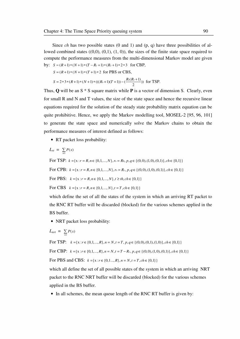
Chapter 4: The Time Space Priority queuing system 90
Since ch has two possible states (0 and 1) and (p, q) have three possibilities of al-
lowed combined states ((0,0), (0,1), (1, 0)), the sizes of the finite state space required to
compute the performance measures from the multi-dimensional Markov model are given
by: ( 1) ( 1) ( 1) ( 1) 2 3c cS R N T R R= + ∗ + ∗ − + ∗ + ∗ ∗ for CBP,
( 1) ( 1) ( 1) 2S R N T= + ∗ + ∗ + ∗ for PBS or CBS,
( 1)2 3 ( 1) ( 1) ((( 1)( 1)) ( ))
2
b b
b
R RS R N R T
+= ∗ ∗ + ∗ + ∗ + + − for TSP.
Thus, Q will be an S * S square matrix while P is a vector of dimension S. Clearly, even
for small R and N and T values, the size of the state space and hence the recursive linear
equations required for the solution of the steady state probability matrix equation can be
quite prohibitive. Hence, we apply the Markov modelling tool, MOSEL-2 [95, 96, 101]
to generate the state space and numerically solve the Markov chains to obtain the
performance measures of interest defined as follows:
• RT packet loss probability:
Lrt = ( )x k
P x∈
∑
For TSP: {x : , {0,1,..., }, , , {(0,0), (1,0), (0,1)}, {0,1}}b bk r R n N r R p q ch= = ∈ = ∈ ∈
For CPB: {x : , {0,1,..., }, , , {(0,0), (1,0), (0,1)}, {0,1}}b ck r R n N r R p q ch= = ∈ = ∈ ∈
For PBS: {x : , {0,1,..., }, , {0,1}}k r R n N t th ch= = ∈ ≥ ∈
For CBS {x : , {0,1,..., }, , {0,1}}k r R n N t T ch= = ∈ = ∈
which define the set of all the states of the system in which an arriving RT packet to
the RNC RT buffer will be discarded (blocked) for the various schemes applied in the
BS buffer.
• NRT packet loss probability:
Lnrt = ( )x k
P x∈
∑
For TSP: {x : {0,1,..., }, , , , {(0,0), (0,1), (1,0)}, {0,1}}k r R n N t T p q ch= ∈ = = ∈ ∈
For CBP: {x : {0,1,..., }, , , , {(0,0), (1,0), (0,1)}, {0,1}}ck r R n N t T R p q ch= ∈ = = − ∈ ∈
For PBS and CBS: {x : {0,1..., }, , , {0,1}}k r R n N t T ch= ∈ = = ∈
which all define the set of all possible states of the system in which an arriving NRT
packet to the RNC NRT buffer will be discarded (blocked) for the various schemes
applied in the BS buffer.
• In all schemes, the mean queue length of the RNC RT buffer is given by:
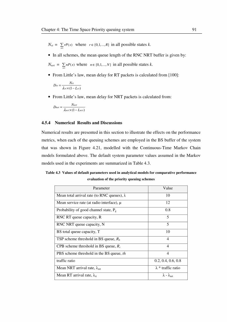
Chapter 4: The Time Space Priority queuing system 91
Nrt = ( )x k
rP x∈
∑ where {0,1,..., }r R∈ in all possible states k.
• In all schemes, the mean queue length of the RNC NRT buffer is given by:
Nnrt = ( )x k
nP x∈
∑ where {0,1,..., }n N∈ in all possible states k.
• From Little’s law, mean delay for RT packets is calculated from [100]:
r(1 )
rtrt
rt t
ND
Lλ=
× −
• From Little’s law, mean delay for NRT packets is calculated from:
r(1 )
nrtnrt
nrt n t
ND
Lλ=
× −
4.5.4 Numerical Results and Discussions
Numerical results are presented in this section to illustrate the effects on the performance
metrics, when each of the queuing schemes are employed in the BS buffer of the system
that was shown in Figure 4.21, modelled with the Continuous-Time Markov Chain
models formulated above. The default system parameter values assumed in the Markov
models used in the experiments are summarized in Table 4.3.
Table 4.3 Values of default parameters used in analytical models for comparative performance
evaluation of the priority queuing schemes
Parameter Value
Mean total arrival rate (to RNC queues), λ 10
Mean service rate (at radio interface), µ 12
Probability of good channel state, Pg 0.8
RNC RT queue capacity, R 5
RNC NRT queue capacity, N 5
BS total queue capacity, T 10
TSP scheme threshold in BS queue, Rb 4
CPB scheme threshold in BS queue, Rc 4
PBS scheme threshold in the BS queue, th 4
traffic ratio 0.2, 0.4, 0.6, 0.8
Mean NRT arrival rate, λnrt λ * traffic ratio
Mean RT arrival rate, λrt λ - λnrt
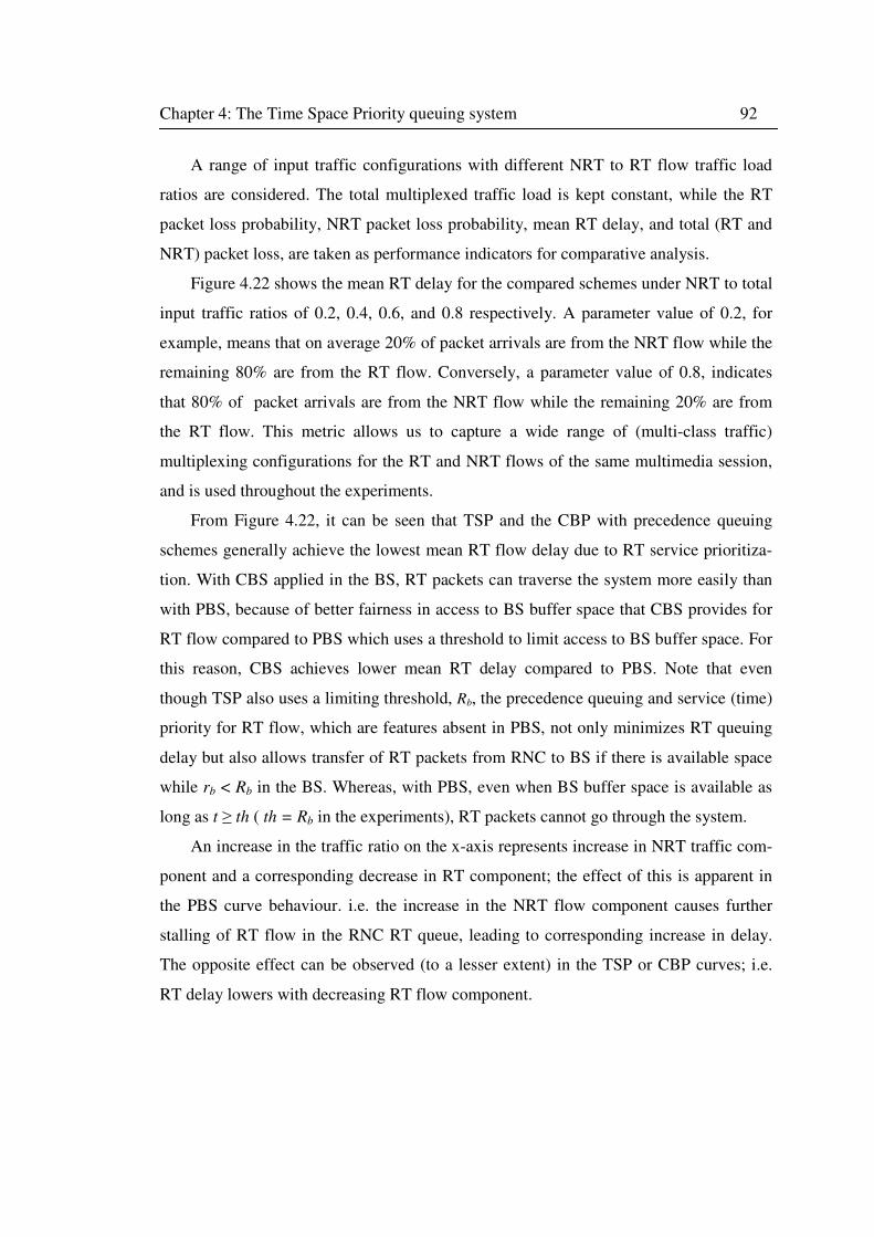
Chapter 4: The Time Space Priority queuing system 92
A range of input traffic configurations with different NRT to RT flow traffic load
ratios are considered. The total multiplexed traffic load is kept constant, while the RT
packet loss probability, NRT packet loss probability, mean RT delay, and total (RT and
NRT) packet loss, are taken as performance indicators for comparative analysis.
Figure 4.22 shows the mean RT delay for the compared schemes under NRT to total
input traffic ratios of 0.2, 0.4, 0.6, and 0.8 respectively. A parameter value of 0.2, for
example, means that on average 20% of packet arrivals are from the NRT flow while the
remaining 80% are from the RT flow. Conversely, a parameter value of 0.8, indicates
that 80% of packet arrivals are from the NRT flow while the remaining 20% are from
the RT flow. This metric allows us to capture a wide range of (multi-class traffic)
multiplexing configurations for the RT and NRT flows of the same multimedia session,
and is used throughout the experiments.
From Figure 4.22, it can be seen that TSP and the CBP with precedence queuing
schemes generally achieve the lowest mean RT flow delay due to RT service prioritiza-
tion. With CBS applied in the BS, RT packets can traverse the system more easily than
with PBS, because of better fairness in access to BS buffer space that CBS provides for
RT flow compared to PBS which uses a threshold to limit access to BS buffer space. For
this reason, CBS achieves lower mean RT delay compared to PBS. Note that even
though TSP also uses a limiting threshold, Rb, the precedence queuing and service (time)
priority for RT flow, which are features absent in PBS, not only minimizes RT queuing
delay but also allows transfer of RT packets from RNC to BS if there is available space
while rb < Rb in the BS. Whereas, with PBS, even when BS buffer space is available as
long as t ≥ th ( th = Rb in the experiments), RT packets cannot go through the system.
An increase in the traffic ratio on the x-axis represents increase in NRT traffic com-
ponent and a corresponding decrease in RT component; the effect of this is apparent in
the PBS curve behaviour. i.e. the increase in the NRT flow component causes further
stalling of RT flow in the RNC RT queue, leading to corresponding increase in delay.
The opposite effect can be observed (to a lesser extent) in the TSP or CBP curves; i.e.
RT delay lowers with decreasing RT flow component.
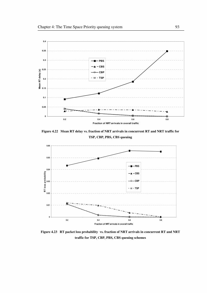
Chapter 4: The Time Space Priority queuing system 93
0
0.05
0.1
0.15
0.2
0.25
0.3
0.35
0.4
0.2 0.4 0.6 0.8
Fraction of NRT arrivals in overall traffic
Me
an
RT
de
lay
(s
)
PBS
CBS
CBP
TSP
Figure 4.22 Mean RT delay vs. fraction of NRT arrivals in concurrent RT and NRT traffic for
TSP, CBP, PBS, CBS queuing
0
0.01
0.02
0.03
0.04
0.05
0.06
0.2 0.4 0.6 0.8
Fraction of NRT arrivals in overall traffic
RT
lo
ss
pro
ba
bil
ity
PBS
CBS
CBP
TSP
Figure 4.23 RT packet loss probability vs. fraction of NRT arrivals in concurrent RT and NRT
traffic for TSP, CBP, PBS, CBS queuing schemes
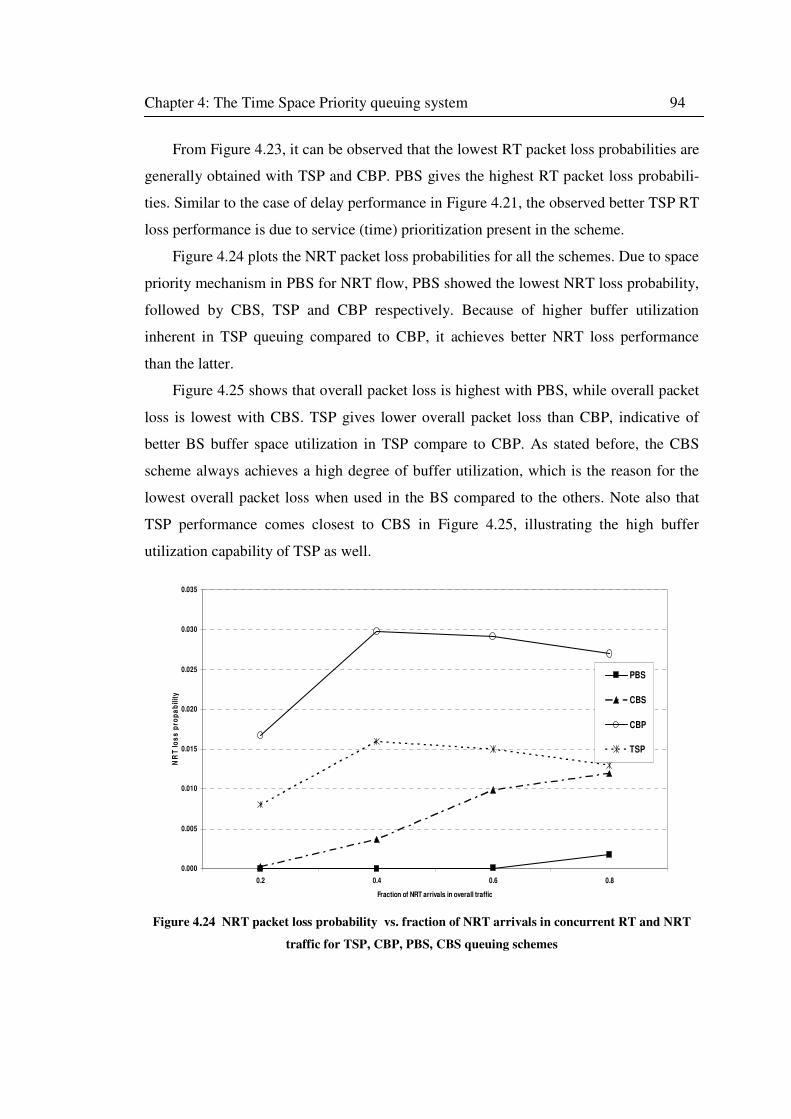
Chapter 4: The Time Space Priority queuing system 94
From Figure 4.23, it can be observed that the lowest RT packet loss probabilities are
generally obtained with TSP and CBP. PBS gives the highest RT packet loss probabili-
ties. Similar to the case of delay performance in Figure 4.21, the observed better TSP RT
loss performance is due to service (time) prioritization present in the scheme.
Figure 4.24 plots the NRT packet loss probabilities for all the schemes. Due to space
priority mechanism in PBS for NRT flow, PBS showed the lowest NRT loss probability,
followed by CBS, TSP and CBP respectively. Because of higher buffer utilization
inherent in TSP queuing compared to CBP, it achieves better NRT loss performance
than the latter.
Figure 4.25 shows that overall packet loss is highest with PBS, while overall packet
loss is lowest with CBS. TSP gives lower overall packet loss than CBP, indicative of
better BS buffer space utilization in TSP compare to CBP. As stated before, the CBS
scheme always achieves a high degree of buffer utilization, which is the reason for the
lowest overall packet loss when used in the BS compared to the others. Note also that
TSP performance comes closest to CBS in Figure 4.25, illustrating the high buffer
utilization capability of TSP as well.
0.000
0.005
0.010
0.015
0.020
0.025
0.030
0.035
0.2 0.4 0.6 0.8
Fraction of NRT arrivals in overall traffic
NR
T l
os
s p
rop
ab
ilit
y
PBS
CBS
CBP
TSP
Figure 4.24 NRT packet loss probability vs. fraction of NRT arrivals in concurrent RT and NRT
traffic for TSP, CBP, PBS, CBS queuing schemes
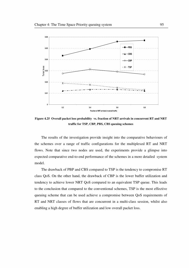
Chapter 4: The Time Space Priority queuing system 95
0
0.01
0.02
0.03
0.04
0.05
0.06
0.2 0.4 0.6 0.8
Fraction of NRT arrivals in overall traffic
To
tal
los
s
PBS
CBS
CBP
TSP
Figure 4.25 Overall packet loss probability vs. fraction of NRT arrivals in concurrent RT and NRT
traffic for TSP, CBP, PBS, CBS queuing schemes
The results of the investigation provide insight into the comparative behaviours of
the schemes over a range of traffic configurations for the multiplexed RT and NRT
flows. Note that since two nodes are used, the experiments provide a glimpse into
expected comparative end-to-end performance of the schemes in a more detailed system
model.
The drawback of PBP and CBS compared to TSP is the tendency to compromise RT
class QoS. On the other hand, the drawback of CBP is the lower buffer utilization and
tendency to achieve lower NRT QoS compared to an equivalent TSP queue. This leads
to the conclusion that compared to the conventional schemes, TSP is the most effective
queuing scheme that can be used achieve a compromise between QoS requirements of
RT and NRT classes of flows that are concurrent in a multi-class session, whilst also
enabling a high degree of buffer utilization and low overall packet loss.
Chapter 4: The Time Space Priority queuing system 96
4.6 Chapter summary
This chapter presented the novel Time Space Priority (TSP) queuing system for buffer
allocation and QoS management of multimedia traffic consisting of multiplexed real-
time (RT) and non-real-time (NRT) classes of flows. The TSP queue is modeled using
M2/M2/1/R, N queue, and a Continuous Time Markov Chain (CTMC) is used to
represent the system behavior from which the impact of traffic and configuration para-
meters on the QoS performance of both flows is studied. The CTMC is generated and
solved using the analytical modelling tool MOSEL-2, and the results are cross-validated
with a discrete event simulation of the M2/M2/1/R, N queuing system using the C
language. The results’ validation are given in Appendix A. The results of the experi-
ments highlight the importance of optimum TSP threshold selection, suggesting that a
small TSP threshold, R, compared to the total buffer capacity, N is preferable from the
viewpoint of joint RT and NRT QoS control. A function known as the WGoS criterion γ,
is derived for calculating an optimum buffer threshold for joint RT and NRT QoS
performance trade-off for a given total buffer capacity and traffic configuration using the
TSP queuing model. Furthermore, in this chapter, an approach for dynamic buffer
threshold optimization using an analytic engine comprising the TSP analytic model and
WGoS function, is suggested.
The chapter also presented a comparative performance evaluation of TSP with exist-
ing conventional queuing disciplines designed to give further insight into the merits and
constraints of TSP and to assess its capability to enable joint RT and NRT QoS control
compared to the conventional queuing disciplines. From the investigation, TSP achieves
high buffer utilization, while proving to be the most effective queuing scheme that can
allow customized preferential treatment to both RT and NRT components of the same
multimedia session, allowing a reasonable compromise between their conflicting QoS
requirements. In the subsequent chapters, TSP-based buffer management algorithms for
user-specific multimedia traffic control in HSDPA system are proposed and evaluated.
97
Chapter 5
Buffer Management for HSDPA
Multimedia Traffic
5.1 Introduction
In the previous chapter, Time-Space Priority (TSP) queuing was introduced and ana-
lyzed. Comparative analytical studies with conventional priority queuing schemes
showed the viability of TSP for joint QoS control and optimization through delay and
loss differentiation for multiplexed real-time (RT) and non-real-time (NRT) services
transmitted over a common channel to an end-user. Furthermore, TSP proved to be
efficient as a queuing strategy in allocation and utilization of the shared buffer resources
between the concurrent RT and NRT flows.
This chapter presents a buffer management scheme based on TSP queuing for mul-
timedia traffic in HSDPA networks. In order to assess the potential performance gain of
the TSP based buffer management scheme in HSDPA, a dynamic network level HSDPA
system simulation model was built and used for the investigation. Comparative perfor-
mance analyses with reference multi-class buffer management schemes demonstrates the
effectiveness of TSP based buffer management for joint QoS control of the real-time and
non-real-time components of the multimedia session in HSDPA. The chapter is orga-
nized as follows. The next section highlights the HSDPA QoS framework that can be
utilized to support Node B buffer management, while section 5.3 discusses the incorpo-
ration of buffer management algorithms into existing HSDPA system. Section 5.4
Chapter 5 Buffer management for HSDPA multimedia traffic 98
presents the HSDPA simulation modelling for the TSP buffer management performance
study, while the results are presented and discussed in section 5.5.
5.2 HSDPA QoS framework
The 3GPP HSDPA specifications do not include specific buffer management algorithms
for Node B operation therefore allowing for network performance optimization through
any implementation the operator may see fit. However, as mentioned earlier in chapter 3,
the Node B utilizes a single shared channel called the High Speed Downlink Shared
Channel (HS-DSCH) for HSDPA users, with buffering of user data in the MAC-hs
protocol sub-layer which allows for inter-user scheduling of data and priority handling
of multiple flows belonging to the same user (see Figure 3.4 of chapter 3).
Data buffering in the Node B MAC-hs layer necessitates buffer management espe-
cially where multiplexed RT and NRT flows are queued for the same user in the same
multimedia session. This is because of the potential impact on end-to-end QoS perfor-
mance of both flows due to the queuing at the radio interface, which presents a
bandwidth bottleneck and time varying UE channel quality. Furthermore, due to the fact
that queuing delays at the air interface nodes typically exceed the transmission delays to
the mobile nodes, (especially when the cell is highly loaded or the UE channel quality
deteriorates), application of buffer management techniques at the radio interface is
particularly crucial to QoS performance enhancement. Additionally, employing buffer
management techniques at the air interface can improve both network and radio resource
utilization efficiency leading to an increase in system capacity.
In order to implement buffer management schemes for multiplexed services, me-
chanisms for QoS differentiation are necessary. In chapter 2, the different traffic classes
(Conversational, Streaming, Interactive and Background) for QoS differentiation were
discussed. HSDPA specifications (3GPP Release 5) defines a flexible framework that
allows the use of these classes and other bearer attributes in implementing QoS control
mechanisms at the air interface (i.e. in the Node B). The HSDPA QoS framework
defines a new QoS interface between the RNC and the Node B to facilitate parameter
mapping, measurement feedback and information exchange for operating the QoS
control mechanisms [74]. The main parameters sent across the QoS interface which are
Chapter 5 Buffer management for HSDPA multimedia traffic 99
set based on the traffic class and other bearer QoS attributes, to be used for MAC-hs
based QoS mechanisms include:
• Guaranteed bit rate (GBR)
• Service priority indicator (SPI)
• Discard timer (DT)
The GBR parameter can be used to guide the MAC-hs to schedule users according
to a target average user bit rate. The SPI parameter indicates the priority of the data flow
and can take integer values in the range 0-15, where a high number indicates high
priority and vice versa. The DT specifies the maximum time a packet is allowed to be
buffered in the Node B’s MAC-hs before it is discarded. It is recommended to set GBR,
SPI, and DT as a function of the Traffic Class (TC) and Traffic Handling Priority (THP)
for each packet flow. For example, suppose SGSN in the core network maps VoIP
services to the conversational TC with THP =1, RNC can set GBR= 16kb/s and use a
high SPI value to indicate relative high priority of VoIP services. For streaming TC, the
HSDPA GBR parameter can be set according to the bit rate requirement specified in the
UMTS bearer attribute for this TC [102]. Similarly, web browsing applications on the
background TC could be assigned GBR = X and a lower SPI to indicate the requirement
to be served with at least X average bit rate but with a relatively lower priority than other
services.
The above examples relate to the use of the parameters for QoS-enabled MAC-hs
scheduling where a single service exists per UE. But while these parameters are availa-
ble for use in the MAC-hs scheduler, they could also be employed in implementing
buffer management algorithms. For example the Guaranteed Bit rate (GBR) and Discard
Timer (DT) parameters are utilized in the enhanced and dynamic buffer management
schemes presented in chapters 6 and 7 respectively.
5.3 Buffer management algorithms in HSDPA MAC-hs
5.3.1 Functions of the MAC-hs buffer management algorithm
According to 3GPP TS 25.321 (MAC specification), the scheduler’s function is to
schedule all UEs within the cell as well as to service priority queues i.e. priority han-
dling. The scheduler schedules MAC-hs SDUs (generated from one or more queued
Chapter 5 Buffer management for HSDPA multimedia traffic 100
MAC-d PDUs) based on information from upper layers. One UE may be associated with
one or more MAC-d flows. Each MAC-d flow contains HS-DSCH MAC-d PDUs for
one or more priority queues. Hence, in our approach, the buffer management algorithm
(BMA) can be considered a sub-function of the MAC-hs scheduler which oversees the
responsibility of handling priorities for multiple flows (priority queues) associated with
the same UE in the MAC-hs. With this approach, classical packets scheduling algo-
rithms such as Max throughput, Max-C/I, proportional fair, M-LWDF, etc. can be
applied for inter-user transmission scheduling while the BMA handles inter-class
transmission prioritization between the RT and NRT flows (through its time priority
policy).
The BMA performs buffer admission control (BAC) on arriving MAC-d PDUs ac-
cording to the priority scheme’s BAC mechanism. The BMA also determines the MAC-
d flow (identifies the UE priority Queue ID) from which the MAC-d PDUs will be
assembled into MAC-hs SDUs for transmission to the UE on a given HARQ entity. If
priority switching is enabled (in the case of a dynamic buffer management scheme like
D-TSP discussed in chapter 7), the priority switching algorithm is consulted to identify
the correct MAC-d flow (Queue ID) for next transmission. The scheduler then schedules
the MAC-d flow on a selected HARQ process, if the scheduling algorithm has allocated
the next transmission opportunity to the UE associated with the MAC-d flow. Thus, the
buffer management algorithm as a sub-entity of the MAC-hs scheduler, is executed on
each of the UE’s MAC-d flows i.e. the priority handling for UE‘s with multiple flows
per session (i.e. multiplexed RT and NRT flows concurrent in the multimedia connec-
tion). The MAC-hs scheduling and priority queuing functionalities are illustrated in
Figure 3.4 of chapter 3. The entire scheduling process for multimedia sessions therefore,
can be viewed as occurring in a logical hierarchy with the BMA performing buffer
admission control and inter-class (inter-flow) scheduling, while the MAC-hs scheduling
performs the inter-UE scheduling according to any of the well known scheduling discip-
lines like Max-C/I, Proportional Fair, etc. This logical scheduling hierarchy is show in
Figure 5.1.
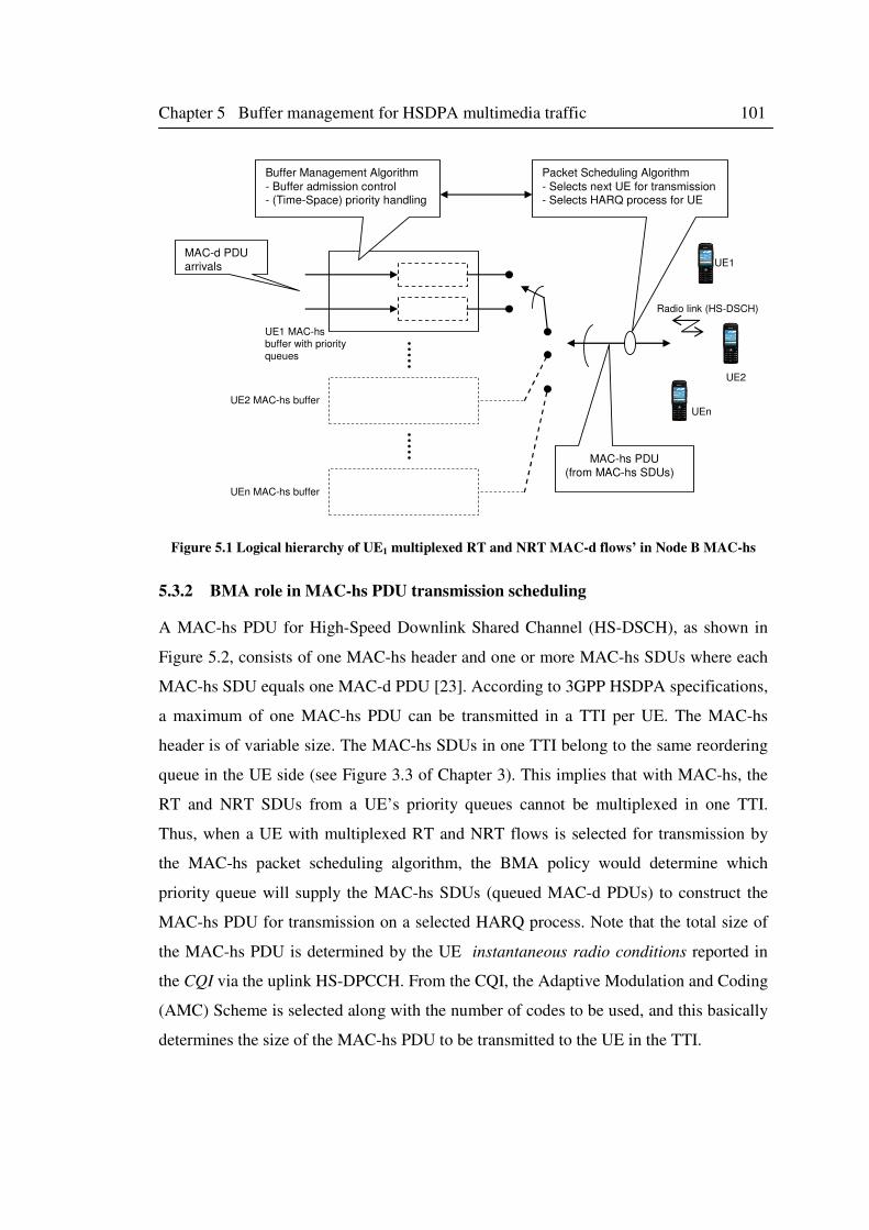
Chapter 5 Buffer management for HSDPA multimedia traffic 101
Radio link (HS-DSCH)
UEn MAC-hs buffer
UE2 MAC-hs buffer
UE1 MAC-hsbuffer with priority
queues
UEn
UE2
UE1MAC-d PDUarrivals
Buffer Management Algorithm
- Buffer admission control- (Time-Space) priority handling
Packet Scheduling Algorithm
- Selects next UE for transmission- Selects HARQ process for UE
MAC-hs PDU(from MAC-hs SDUs)
Figure 5.1 Logical hierarchy of UE1 multiplexed RT and NRT MAC-d flows’ in Node B MAC-hs
5.3.2 BMA role in MAC-hs PDU transmission scheduling
A MAC-hs PDU for High-Speed Downlink Shared Channel (HS-DSCH), as shown in
Figure 5.2, consists of one MAC-hs header and one or more MAC-hs SDUs where each
MAC-hs SDU equals one MAC-d PDU [23]. According to 3GPP HSDPA specifications,
a maximum of one MAC-hs PDU can be transmitted in a TTI per UE. The MAC-hs
header is of variable size. The MAC-hs SDUs in one TTI belong to the same reordering
queue in the UE side (see Figure 3.3 of Chapter 3). This implies that with MAC-hs, the
RT and NRT SDUs from a UE’s priority queues cannot be multiplexed in one TTI.
Thus, when a UE with multiplexed RT and NRT flows is selected for transmission by
the MAC-hs packet scheduling algorithm, the BMA policy would determine which
priority queue will supply the MAC-hs SDUs (queued MAC-d PDUs) to construct the
MAC-hs PDU for transmission on a selected HARQ process. Note that the total size of
the MAC-hs PDU is determined by the UE instantaneous radio conditions reported in
the CQI via the uplink HS-DPCCH. From the CQI, the Adaptive Modulation and Coding
(AMC) Scheme is selected along with the number of codes to be used, and this basically
determines the size of the MAC-hs PDU to be transmitted to the UE in the TTI.
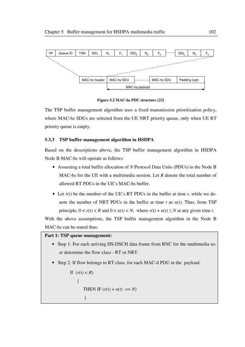
Chapter 5 Buffer management for HSDPA multimedia traffic 102
MAC-hs header MAC-hs SDU MAC-hs SDU Padding (opt)
MAC-hs payload
VF Queue ID TSN SID1 N1 F1 SID2 N2 F2 SIDk Nk Fk
Figure 5.2 MAC-hs PDU structure [23]
The TSP buffer management algorithm uses a fixed transmission prioritization policy,
where MAC-hs SDUs are selected from the UE NRT priority queue, only when UE RT
priority queue is empty.
5.3.3 TSP buffer management algorithm in HSDPA
Based on the descriptions above, the TSP buffer management algorithm in HSDPA
Node B MAC-hs will operate as follows:
• Assuming a total buffer allocation of N Protocol Data Units (PDUs) in the Node B
MAC-hs for the UE with a multimedia session. Let R denote the total number of
allowed RT PDUs in the UE’s MAC-hs buffer.
• Let r(t) be the number of the UE’s RT PDUs in the buffer at time t, while we de-
note the number of NRT PDUs in the buffer at time t as n(t). Thus, from TSP
principle, 0 < r(t) < R and 0 < n(t) < N, where r(t) + n(t) ≤ N at any given time t.
With the above assumptions, the TSP buffer management algorithm in the Node B
MAC-hs can be stated thus:
Part 1: TSP queue management:
• Step 1: For each arriving HS-DSCH data frame from RNC for the multimedia us-
er determine the flow class - RT or NRT.
• Step 2: If flow belongs to RT class, for each MAC-d PDU in the payload:
If (r(t) < R)
{
THEN IF (r(t) + n(t) == N)
{
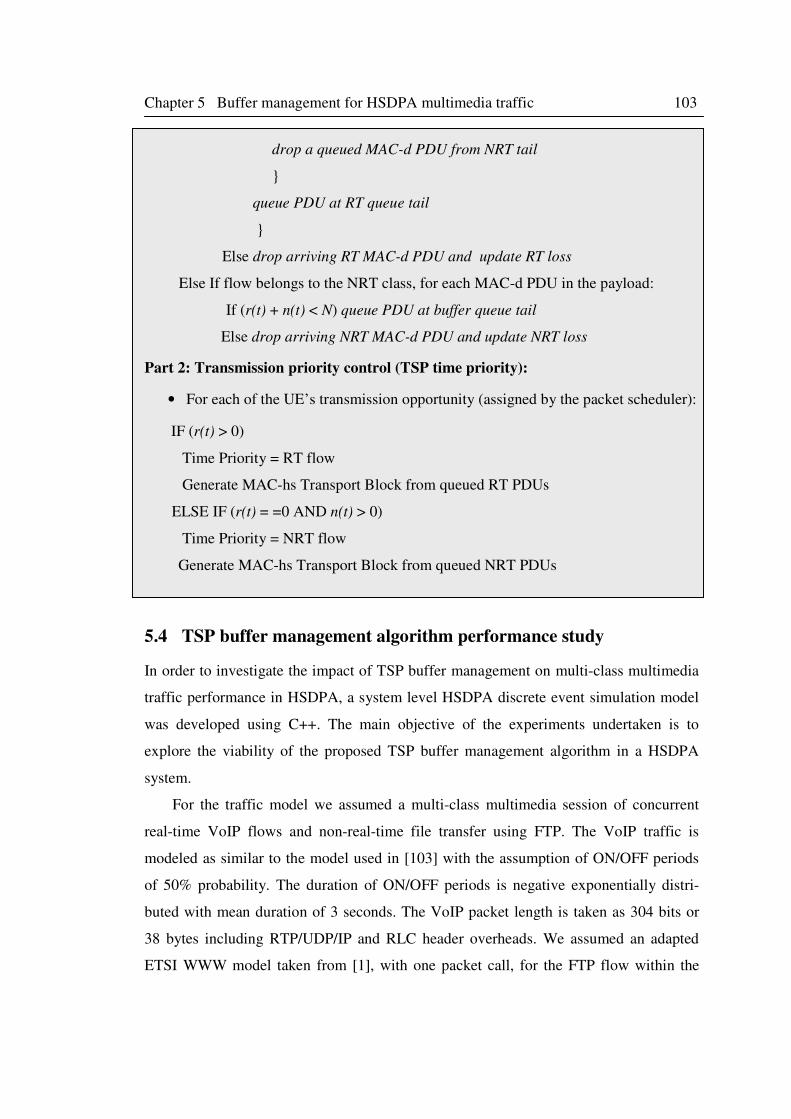
Chapter 5 Buffer management for HSDPA multimedia traffic 103
drop a queued MAC-d PDU from NRT tail
}
queue PDU at RT queue tail
}
Else drop arriving RT MAC-d PDU and update RT loss
Else If flow belongs to the NRT class, for each MAC-d PDU in the payload:
If (r(t) + n(t) < N) queue PDU at buffer queue tail
Else drop arriving NRT MAC-d PDU and update NRT loss
Part 2: Transmission priority control (TSP time priority):
• For each of the UE’s transmission opportunity (assigned by the packet scheduler):
IF (r(t) > 0)
Time Priority = RT flow
Generate MAC-hs Transport Block from queued RT PDUs
ELSE IF (r(t) = =0 AND n(t) > 0)
Time Priority = NRT flow
Generate MAC-hs Transport Block from queued NRT PDUs
5.4 TSP buffer management algorithm performance study
In order to investigate the impact of TSP buffer management on multi-class multimedia
traffic performance in HSDPA, a system level HSDPA discrete event simulation model
was developed using C++. The main objective of the experiments undertaken is to
explore the viability of the proposed TSP buffer management algorithm in a HSDPA
system.
For the traffic model we assumed a multi-class multimedia session of concurrent
real-time VoIP flows and non-real-time file transfer using FTP. The VoIP traffic is
modeled as similar to the model used in [103] with the assumption of ON/OFF periods
of 50% probability. The duration of ON/OFF periods is negative exponentially distri-
buted with mean duration of 3 seconds. The VoIP packet length is taken as 304 bits or
38 bytes including RTP/UDP/IP and RLC header overheads. We assumed an adapted
ETSI WWW model taken from [1], with one packet call, for the FTP flow within the

Chapter 5 Buffer management for HSDPA multimedia traffic 104
concurrent multi-class multimedia traffic. Thus FTP average packet size is assumed to
be 480 bytes with exponentially distribute packet sizes. The inter-arrival times are
geometrically distributed, corresponding to the download bit rate allocated and main-
tained throughout the multimedia session.
Packets are assumed to arrive from the core network to the radio access network
without any loss. For the Radio Access Network, a single HSDPA cell served by a Node
B under the control of an RNC with the concurrent VoIP and FTP downlink traffic
towards an end user (UE) was modelled.
Radio propagation was modeled using ITU R path loss model and lognormal sha-
dowing with std. deviation σ = 8 dB. The path loss model used is taken from [104]:
L = 40 log10 R + 30 log10 f + 39 (5.1)
where f is the WCDMA carrier frequency i.e. 2GHz, and R is the distance of the mobile
from the base station in kilometers.
The lognormal shadowing in logarithmic scale is characterized by a Gaussian distribu-
tion N (0, σ) with Gaussian random variable of mean 0 and σ = 8 [105]. The shadowing
value is updated every 2ms. Due to the slow fading process versus distance, adjacent
shadow fading values are correlated [106]. Thus the following correlation model is
considered for shadow fading [104]:
C(d) = 2-d/dcor
(5.2)
where C(d) is a normalized autocorrelation function of shadowing when decorrelation
length is given by dcor and the moving distance of the mobile after the last calculation
of shadowing is d. Basically, the shadowing effect is represented by [104]:
S = C(d) * S' + 1- [C(d)]2 * N (0, σ) (5.3)
S is the shadowing value in dB updated with the last calculated value S'. In the simula-
tion dcor is set to 5 meters [106].
Total Node B transmission power is assumed to be 15 W, while the allocated HS-
PDSCH power was 7W. The terminal is assumed to be at 0.6 km from the base station
and moving away linearly at 3km/h. The instantaneous throughput towards the UE is
determined by transport block size (TBS) which is governed by the Adaptive modulation
and coding (AMC) functionality. We assumed that six AMC schemes are available and
selected based on the reported channel quality (the instantaneous Signal-to-Interference
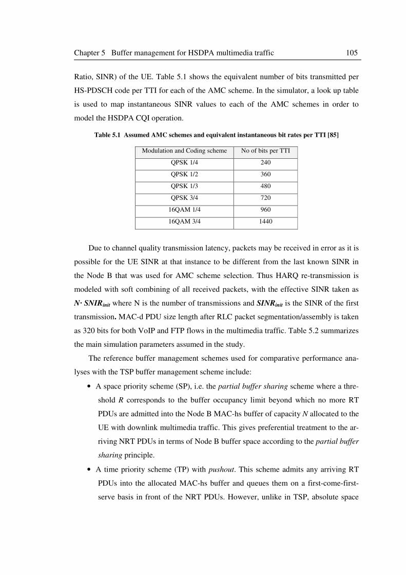
Chapter 5 Buffer management for HSDPA multimedia traffic 105
Ratio, SINR) of the UE. Table 5.1 shows the equivalent number of bits transmitted per
HS-PDSCH code per TTI for each of the AMC scheme. In the simulator, a look up table
is used to map instantaneous SINR values to each of the AMC schemes in order to
model the HSDPA CQI operation.
Table 5.1 Assumed AMC schemes and equivalent instantaneous bit rates per TTI [85]
Modulation and Coding scheme No of bits per TTI
QPSK 1/4 240
QPSK 1/2 360
QPSK 1/3 480
QPSK 3/4 720
16QAM 1/4 960
16QAM 3/4 1440
Due to channel quality transmission latency, packets may be received in error as it is
possible for the UE SINR at that instance to be different from the last known SINR in
the Node B that was used for AMC scheme selection. Thus HARQ re-transmission is
modeled with soft combining of all received packets, with the effective SINR taken as
N· SNIRinit where N is the number of transmissions and SINRinit is the SINR of the first
transmission. MAC-d PDU size length after RLC packet segmentation/assembly is taken
as 320 bits for both VoIP and FTP flows in the multimedia traffic. Table 5.2 summarizes
the main simulation parameters assumed in the study.
The reference buffer management schemes used for comparative performance ana-
lyses with the TSP buffer management scheme include:
• A space priority scheme (SP), i.e. the partial buffer sharing scheme where a thre-
shold R corresponds to the buffer occupancy limit beyond which no more RT
PDUs are admitted into the Node B MAC-hs buffer of capacity N allocated to the
UE with downlink multimedia traffic. This gives preferential treatment to the ar-
riving NRT PDUs in terms of Node B buffer space according to the partial buffer
sharing principle.
• A time priority scheme (TP) with pushout. This scheme admits any arriving RT
PDUs into the allocated MAC-hs buffer and queues them on a first-come-first-
serve basis in front of the NRT PDUs. However, unlike in TSP, absolute space
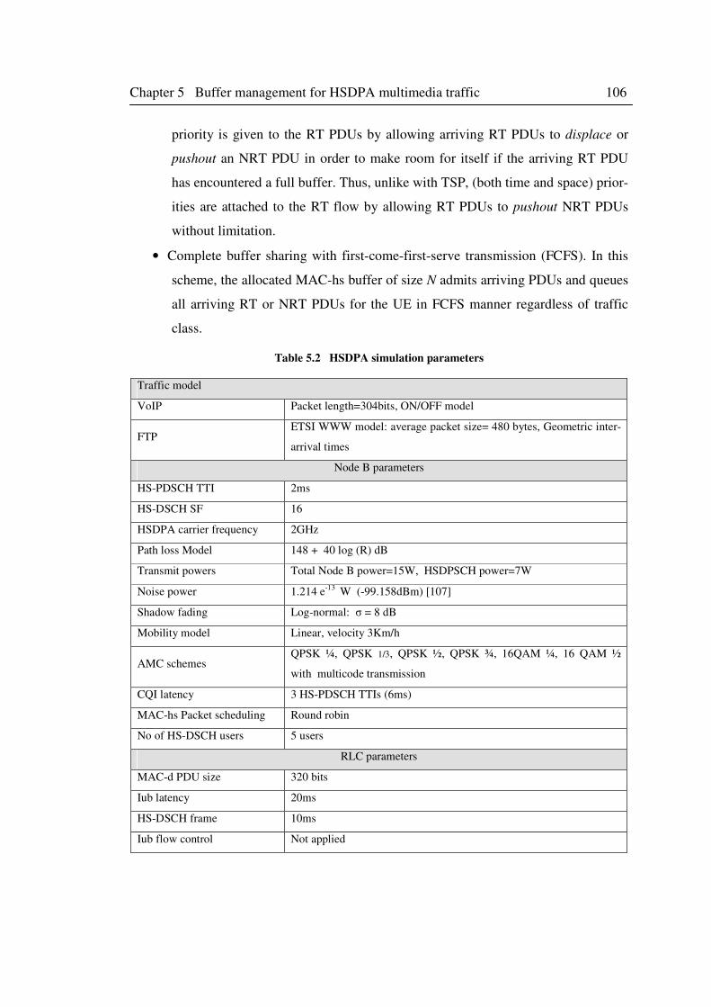
Chapter 5 Buffer management for HSDPA multimedia traffic 106
priority is given to the RT PDUs by allowing arriving RT PDUs to displace or
pushout an NRT PDU in order to make room for itself if the arriving RT PDU
has encountered a full buffer. Thus, unlike with TSP, (both time and space) prior-
ities are attached to the RT flow by allowing RT PDUs to pushout NRT PDUs
without limitation.
• Complete buffer sharing with first-come-first-serve transmission (FCFS). In this
scheme, the allocated MAC-hs buffer of size N admits arriving PDUs and queues
all arriving RT or NRT PDUs for the UE in FCFS manner regardless of traffic
class.
Table 5.2 HSDPA simulation parameters
Traffic model
VoIP Packet length=304bits, ON/OFF model
FTP ETSI WWW model: average packet size= 480 bytes, Geometric inter-
arrival times
Node B parameters
HS-PDSCH TTI 2ms
HS-DSCH SF 16
HSDPA carrier frequency 2GHz
Path loss Model 148 + 40 log (R) dB
Transmit powers Total Node B power=15W, HSDPSCH power=7W
Noise power 1.214 e-13
W (-99.158dBm) [107]
Shadow fading Log-normal: σ = 8 dB
Mobility model Linear, velocity 3Km/h
AMC schemes QPSK ¼, QPSK 1/3, QPSK ½, QPSK ¾, 16QAM ¼, 16 QAM ½
with multicode transmission
CQI latency 3 HS-PDSCH TTIs (6ms)
MAC-hs Packet scheduling Round robin
No of HS-DSCH users 5 users
RLC parameters
MAC-d PDU size 320 bits
Iub latency 20ms
HS-DSCH frame 10ms
Iub flow control Not applied
Chapter 5 Buffer management for HSDPA multimedia traffic 107
5.5 Results and discussions
This section presents the results of experiments conducted using the HSDPA simulation
model. A multimedia session consisting of conversational and background traffic is
simulated. Thus, the scenarios models a UE assumed to be having a ‘live’ VoIP conver-
sation with an external source whilst simultaneously downloading a file via FTP during
the same multimedia session. We investigate the loss and delay performance of the real-
time (VoIP) and non real-time (FTP) flows by varying the data arrival rate of the FTP
flows in the mixed multimedia traffic scenario. Four scenarios are examined, each with
different FTP source rates, in order to observe the impact of NRT traffic load variation
on the performance measures for both VoIP and FTP flows in the UE’s multimedia
session. Performance measures are taken at FTP data rates of 16, 32, 44, 56 and 64 kbps
respectively. The results presented are for the multimedia user under consideration. A
total of 5 users are assumed to be scheduled by the MAC-hs packet scheduler on the HS-
DSCH using round robin scheduling so as to enable fairness in transmission time alloca-
tion between the users. The buffer parameters used in the simulation are given in Table
5.2.
Table 5.3 Multimedia UE MAC-hs buffer parameters for simulation study
Scheme MAC-hs buffer parameters
FCFS Total buffer capacity=20
SP Total buffer capacity=20
Partial buffer sharing threshold=4
TP Total buffer capacity=20
TSP Total buffer capacity=20
Time-Space priority threshold=4
5.5.1 VoIP performance in the mixed traffic
The impact of the NRT traffic load variation (represented as various FTP download
rates) on VoIP performance is shown in Figures 5.3 and 5.4. Results are presented for
FCFS, TP, SP and TSP buffer management schemes for comparative analysis. The
buffer parameters used in the simulation are as given in Table 5.3.
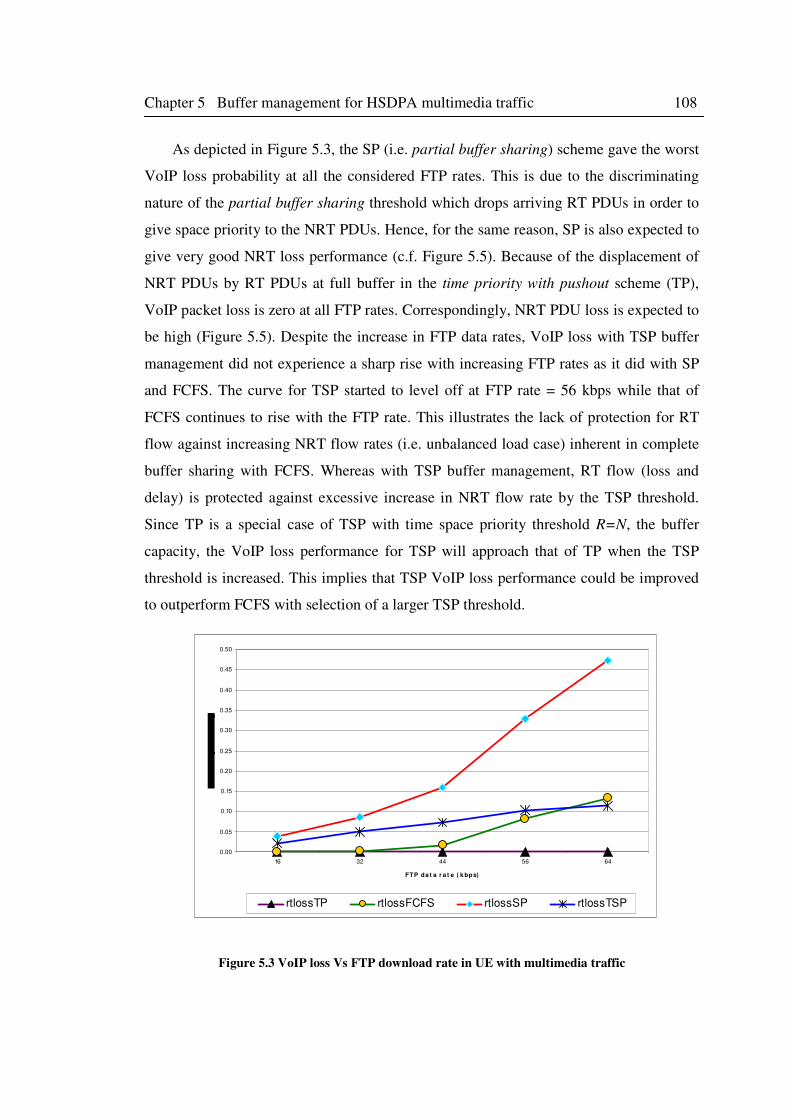
Chapter 5 Buffer management for HSDPA multimedia traffic 108
As depicted in Figure 5.3, the SP (i.e. partial buffer sharing) scheme gave the worst
VoIP loss probability at all the considered FTP rates. This is due to the discriminating
nature of the partial buffer sharing threshold which drops arriving RT PDUs in order to
give space priority to the NRT PDUs. Hence, for the same reason, SP is also expected to
give very good NRT loss performance (c.f. Figure 5.5). Because of the displacement of
NRT PDUs by RT PDUs at full buffer in the time priority with pushout scheme (TP),
VoIP packet loss is zero at all FTP rates. Correspondingly, NRT PDU loss is expected to
be high (Figure 5.5). Despite the increase in FTP data rates, VoIP loss with TSP buffer
management did not experience a sharp rise with increasing FTP rates as it did with SP
and FCFS. The curve for TSP started to level off at FTP rate = 56 kbps while that of
FCFS continues to rise with the FTP rate. This illustrates the lack of protection for RT
flow against increasing NRT flow rates (i.e. unbalanced load case) inherent in complete
buffer sharing with FCFS. Whereas with TSP buffer management, RT flow (loss and
delay) is protected against excessive increase in NRT flow rate by the TSP threshold.
Since TP is a special case of TSP with time space priority threshold R=N, the buffer
capacity, the VoIP loss performance for TSP will approach that of TP when the TSP
threshold is increased. This implies that TSP VoIP loss performance could be improved
to outperform FCFS with selection of a larger TSP threshold.
0.00
0.05
0.10
0.15
0.20
0.25
0.30
0.35
0.40
0.45
0.50
16 32 44 56 64
FTP da t a r a t e ( k bps)
rtlossTP rtlossFCFS rtlossSP rtlossTSP
Figure 5.3 VoIP loss Vs FTP download rate in UE with multimedia traffic
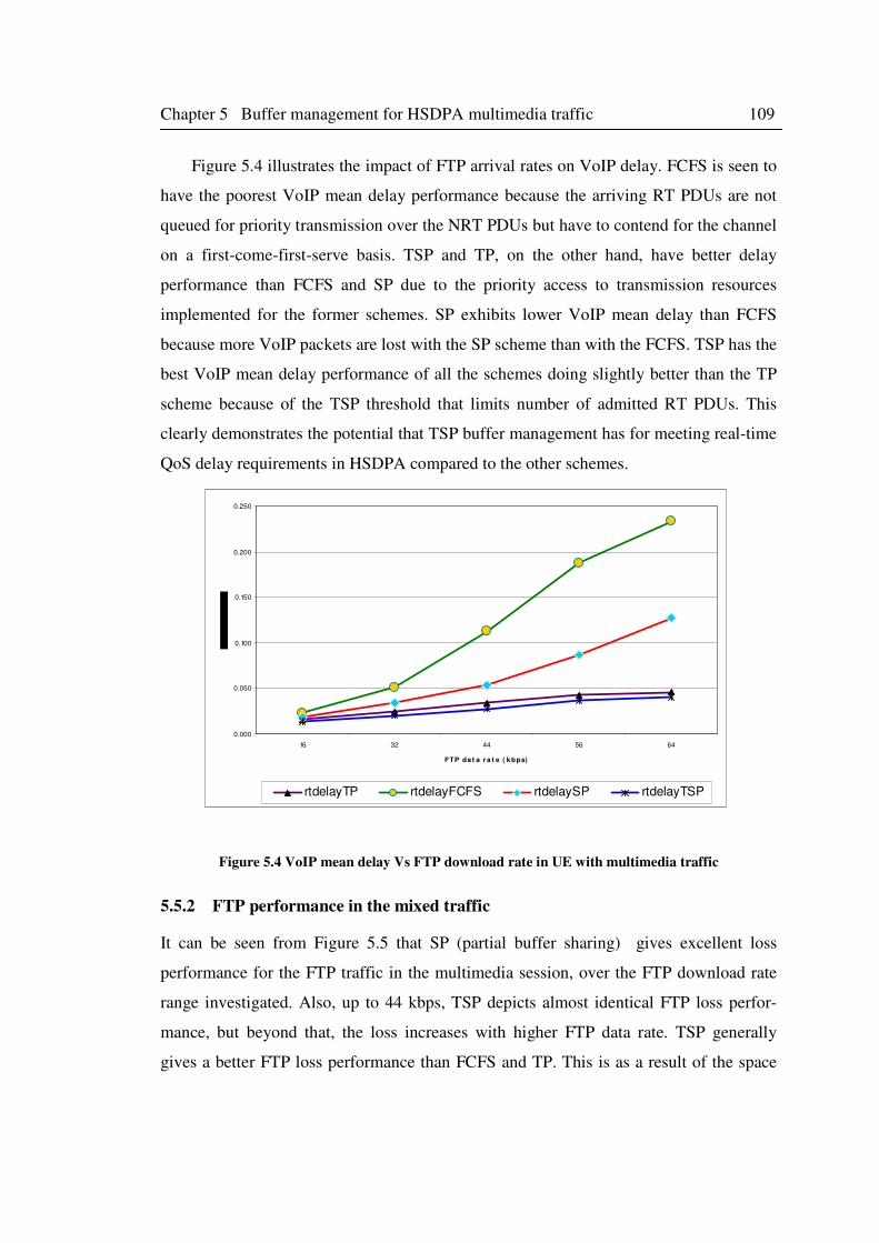
Chapter 5 Buffer management for HSDPA multimedia traffic 109
Figure 5.4 illustrates the impact of FTP arrival rates on VoIP delay. FCFS is seen to
have the poorest VoIP mean delay performance because the arriving RT PDUs are not
queued for priority transmission over the NRT PDUs but have to contend for the channel
on a first-come-first-serve basis. TSP and TP, on the other hand, have better delay
performance than FCFS and SP due to the priority access to transmission resources
implemented for the former schemes. SP exhibits lower VoIP mean delay than FCFS
because more VoIP packets are lost with the SP scheme than with the FCFS. TSP has the
best VoIP mean delay performance of all the schemes doing slightly better than the TP
scheme because of the TSP threshold that limits number of admitted RT PDUs. This
clearly demonstrates the potential that TSP buffer management has for meeting real-time
QoS delay requirements in HSDPA compared to the other schemes.
0.000
0.050
0.100
0.150
0.200
0.250
16 32 44 56 64
FTP da t a r a t e ( k bps)
rtdelayTP rtdelayFCFS rtdelaySP rtdelayTSP
Figure 5.4 VoIP mean delay Vs FTP download rate in UE with multimedia traffic
5.5.2 FTP performance in the mixed traffic
It can be seen from Figure 5.5 that SP (partial buffer sharing) gives excellent loss
performance for the FTP traffic in the multimedia session, over the FTP download rate
range investigated. Also, up to 44 kbps, TSP depicts almost identical FTP loss perfor-
mance, but beyond that, the loss increases with higher FTP data rate. TSP generally
gives a better FTP loss performance than FCFS and TP. This is as a result of the space
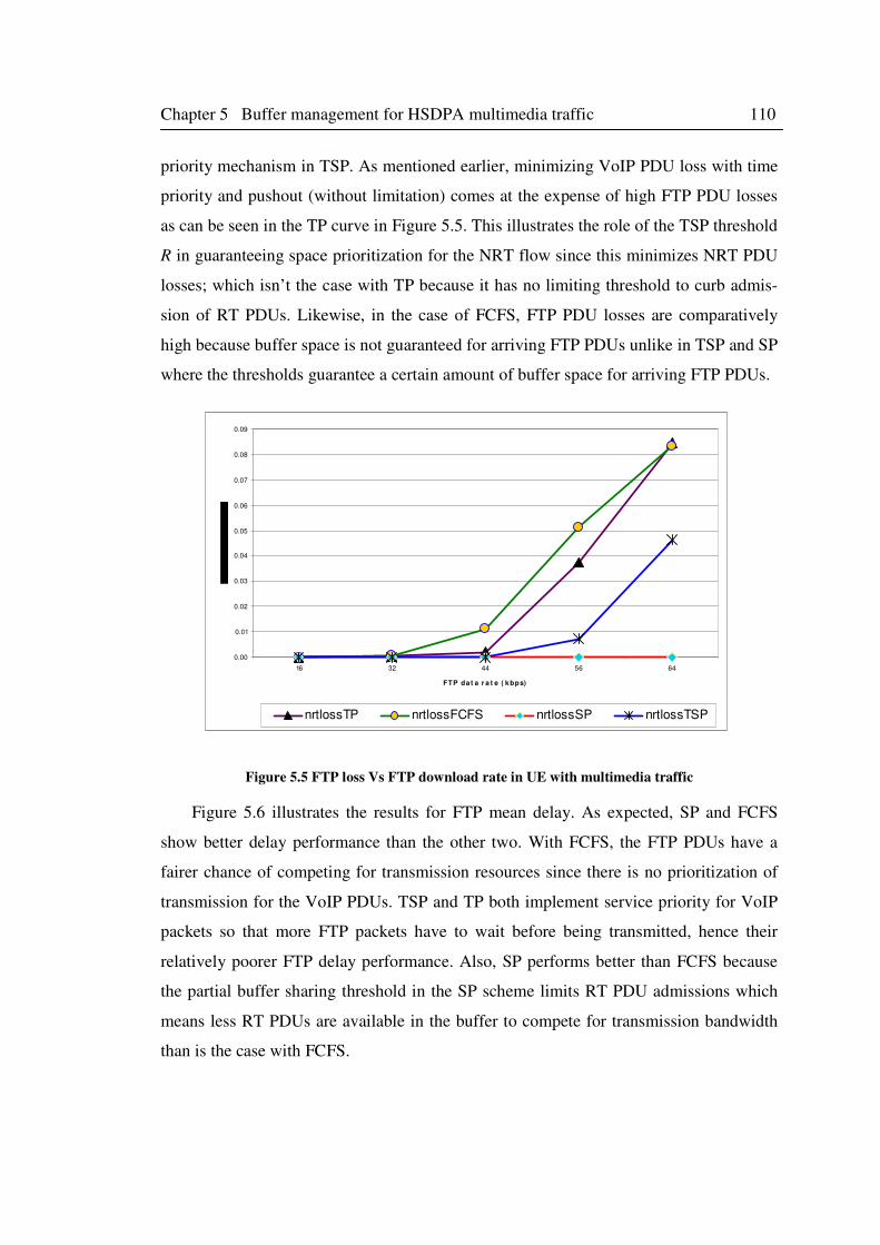
Chapter 5 Buffer management for HSDPA multimedia traffic 110
priority mechanism in TSP. As mentioned earlier, minimizing VoIP PDU loss with time
priority and pushout (without limitation) comes at the expense of high FTP PDU losses
as can be seen in the TP curve in Figure 5.5. This illustrates the role of the TSP threshold
R in guaranteeing space prioritization for the NRT flow since this minimizes NRT PDU
losses; which isn’t the case with TP because it has no limiting threshold to curb admis-
sion of RT PDUs. Likewise, in the case of FCFS, FTP PDU losses are comparatively
high because buffer space is not guaranteed for arriving FTP PDUs unlike in TSP and SP
where the thresholds guarantee a certain amount of buffer space for arriving FTP PDUs.
0.00
0.01
0.02
0.03
0.04
0.05
0.06
0.07
0.08
0.09
16 32 44 56 64
FTP da t a r a t e ( k bps)
nrtlossTP nrtlossFCFS nrtlossSP nrtlossTSP
Figure 5.5 FTP loss Vs FTP download rate in UE with multimedia traffic
Figure 5.6 illustrates the results for FTP mean delay. As expected, SP and FCFS
show better delay performance than the other two. With FCFS, the FTP PDUs have a
fairer chance of competing for transmission resources since there is no prioritization of
transmission for the VoIP PDUs. TSP and TP both implement service priority for VoIP
packets so that more FTP packets have to wait before being transmitted, hence their
relatively poorer FTP delay performance. Also, SP performs better than FCFS because
the partial buffer sharing threshold in the SP scheme limits RT PDU admissions which
means less RT PDUs are available in the buffer to compete for transmission bandwidth
than is the case with FCFS.
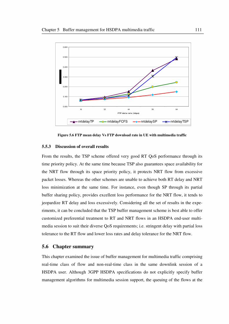
Chapter 5 Buffer management for HSDPA multimedia traffic 111
0.000
0.100
0.200
0.300
0.400
0.500
0.600
16 32 44 56 64
FTP da t a r a t e ( k bps)
nrtdelayTP nrtdelayFCFS nrtdelaySP nrtdelayTSP
Figure 5.6 FTP mean delay Vs FTP download rate in UE with multimedia traffic
5.5.3 Discussion of overall results
From the results, the TSP scheme offered very good RT QoS performance through its
time priority policy. At the same time because TSP also guarantees space availability for
the NRT flow through its space priority policy, it protects NRT flow from excessive
packet losses. Whereas the other schemes are unable to achieve both RT delay and NRT
loss minimization at the same time. For instance, even though SP through its partial
buffer sharing policy, provides excellent loss performance for the NRT flow, it tends to
jeopardize RT delay and loss excessively. Considering all the set of results in the expe-
riments, it can be concluded that the TSP buffer management scheme is best able to offer
customized preferential treatment to RT and NRT flows in an HSDPA end-user multi-
media session to suit their diverse QoS requirements; i.e. stringent delay with partial loss
tolerance to the RT flow and lower loss rates and delay tolerance for the NRT flow.
5.6 Chapter summary
This chapter examined the issue of buffer management for multimedia traffic comprising
real-time class of flow and non-real-time class in the same downlink session of a
HSDPA user. Although 3GPP HSDPA specifications do not explicitly specify buffer
management algorithms for multimedia session support, the queuing of the flows at the
Chapter 5 Buffer management for HSDPA multimedia traffic 112
air interface, makes buffer management an essential QoS enhancing technique. The
solution proposed in this chapter does not require modification to the HSDPA protocol
architecture. Instead, existing HSDPA mechanisms are used to provide per-user buffer
management as a sub-function of the MAC-hs packet scheduling functionality. The
packet scheduler selects the eligible user for transmission allocation according to a
specified packet scheduling discipline, while the (time and space) priority handling for
arriving flows of the user is performed by the buffer management algorithm.
The Time Space Priority buffer management algorithm, which is based on the Time
Space Priority queuing system analyzed in chapter 4, was presented and investigated in
the chapter. A simplified HSDPA discrete event simulation model with VoIP and FTP
flows characterizing an assumed multimedia session is used to compare the performance
of TSP buffer management with other schemes. The results show that applying TSP
based buffer management for QoS control in a HSDPA Node buffer allocated to a
multimedia user with concurrent real-time and non-real-time flows, is effective in
minimizing real-time queuing delay while also minimizing the non-real-time flow losses
through space prioritization. Thus, TSP based buffer management is an effective scheme
for joint QoS control of real-time and non-real-time flows concurrent in a HSDPA
multimedia session. The next chapter explores the extension of the TSP buffer manage-
ment scheme with flow control mechanisms within the HSDPA Radio Access Network
(RAN) in order to alleviate MAC-hs buffer overflow for enhanced end-to-end traffic
performance gains during the multimedia session.
113
Chapter 6
Enhanced Buffer Management for
HSDPA Multimedia Traffic
6.1 Introduction
In chapters 4 and 5, performance evaluation of Time-Space Priority (TSP) queuing
system and buffer management were undertaken. The studies have demonstrated the
viability of TSP for joint QoS control and optimization through delay and loss differen-
tiation for multiplexed RT and NRT services transmitted over a common channel to an
end-user. Furthermore, TSP proved to be efficient in allocation and utilization of the
shared buffer resources between the concurrent RT and NRT flows.
This chapter presents an enhanced buffer management scheme based on the TSP
queuing for multimedia traffic in HSDPA networks. The scheme, termed E-TSP (En-
hanced Time Space Priority) buffer management, incorporates mechanisms for flow
control to mitigate potential buffer overflow in order to further minimize packet losses in
the radio access network as well as curb excessive buffer queuing delays. Consequently,
enhancement of the performance of higher layer protocols, most especially TCP is
envisaged. Thus, E-TSP flow control mechanism in the HSDPA radio access network, is
designed to improve end-to-end throughput performance for the multimedia traffic,
whilst enabling efficient utilization of radio link resources. E-TSP is an enhancement of
the TSP buffer management algorithm for HSDPA studied in chapter 5.
Chapter 6: Enhanced buffer management for HSDPA multimedia traffic 114
In order to assess the potential end-to-end performance gain of E-TSP, a dynamic
system-level HSDPA system simulation model was built using OPNET modeler and
used to investigate E-TSP under various HSDPA channel loads and multiplexed service
scenario of a mixed VoIP and TCP-based FTP user session.
The chapter is organized as follows. The next section explains the Iub flow control
protocol in HSDPA, while section 6.3 presents the proposed E-TSP buffer management
algorithm that employs the Iub flow control protocol. An experiment via system level
HSDPA simulations to study the potential end-to-end performance gains achievable with
E-TSP is presented in section 6.4. Finally, the chapter is concluded with a summary in
section 6.5.
6.2 HSDPA Iub flow control
An important functionality specified in 3GPP standards for the Node B MAC-hs opera-
tion is the flow control mechanism, which uses a credit-based system to regulate data
flow over the Iub interface between the RNC and Node B. The Iub interface between
Node B and RNC in HSDPA, requires the flow control mechanisms to ensure that Node
B buffers are used properly and there is no data loss due to Node B buffer overflow [20].
The HS-DSCH flow control mechanism is described in the 3GPP specifications [86] and
is known as a credit-based flow control system.
Some studies on HSDPA performance e.g. [108], [109], [110], [111], indicate that
HSDPA Iub flow control impacts significantly on MAC-hs packet scheduler perfor-
mance, radio link utilization, and the resulting application end-to-end throughput. These
studies however, did not address Iub credit-allocation for flow control of UE traffic
where MAC-hs multiple classes of flows exist. Hence, the Enhanced Time Space
Priority (E-TSP) buffer management scheme proposed in this chapter incorporates a
credit-based flow control algorithm designed for flow control of multiplexed RT and
NRT flows (PDUs) arriving at the Node B MAC-hs queues associated with the multime-
dia UE. The proposed credit allocation algorithm is designed to account for HS-DSCH
load, the specific UE’s radio channel quality and buffer occupancy. Recall that for
reliable transmission, NRT class PDUs are transmitted with Acknowledged Mode (AM)
configuration of the RLC protocol in the RNC, and usually with TCP transport protocol
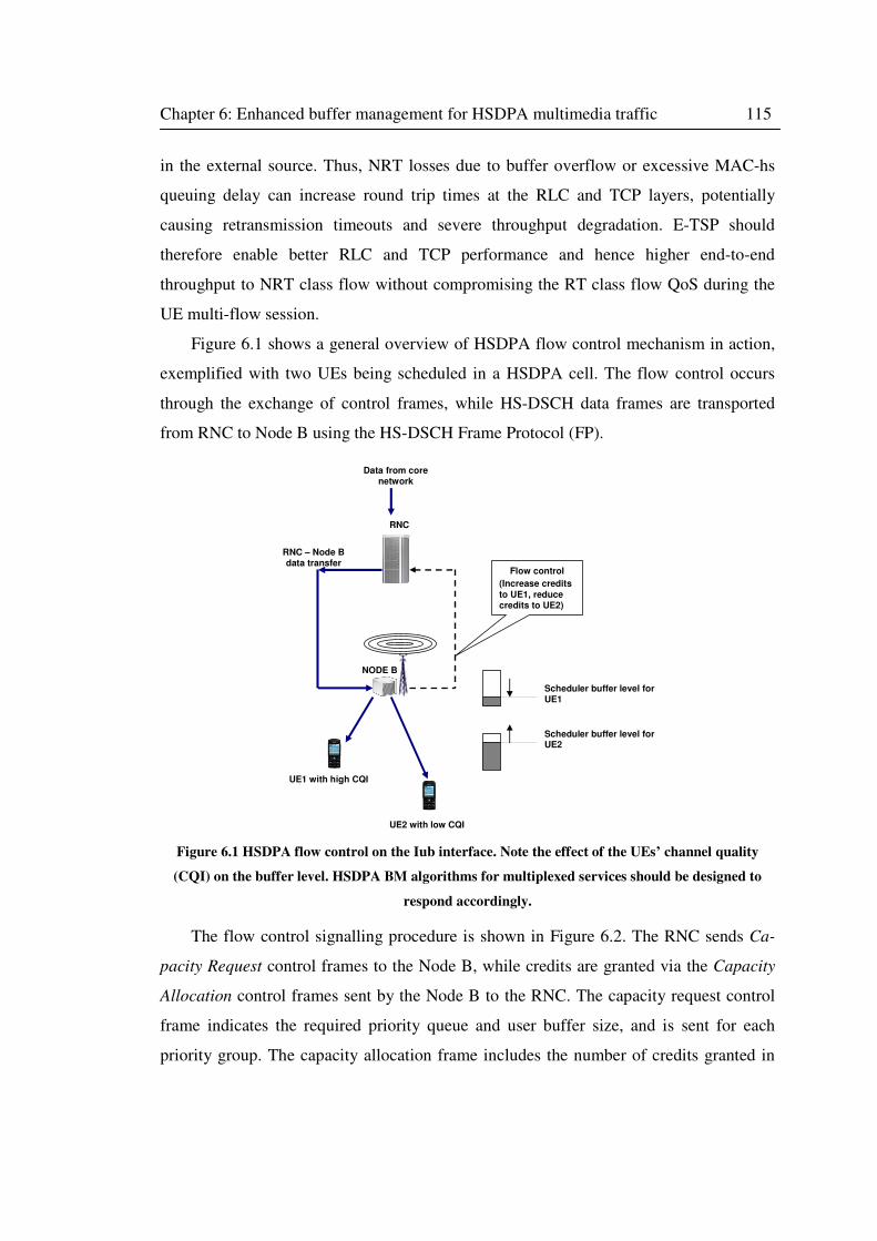
Chapter 6: Enhanced buffer management for HSDPA multimedia traffic 115
in the external source. Thus, NRT losses due to buffer overflow or excessive MAC-hs
queuing delay can increase round trip times at the RLC and TCP layers, potentially
causing retransmission timeouts and severe throughput degradation. E-TSP should
therefore enable better RLC and TCP performance and hence higher end-to-end
throughput to NRT class flow without compromising the RT class flow QoS during the
UE multi-flow session.
Figure 6.1 shows a general overview of HSDPA flow control mechanism in action,
exemplified with two UEs being scheduled in a HSDPA cell. The flow control occurs
through the exchange of control frames, while HS-DSCH data frames are transported
from RNC to Node B using the HS-DSCH Frame Protocol (FP).
NODE B
RNC – Node B data transfer
Scheduler buffer level for UE1
Scheduler buffer level for UE2
Flow control
(Increase credits
to UE1, reduce credits to UE2)
UE1 with high CQI
UE2 with low CQI
RNC
Data from core network
Figure 6.1 HSDPA flow control on the Iub interface. Note the effect of the UEs’ channel quality
(CQI) on the buffer level. HSDPA BM algorithms for multiplexed services should be designed to
respond accordingly.
The flow control signalling procedure is shown in Figure 6.2. The RNC sends Ca-
pacity Request control frames to the Node B, while credits are granted via the Capacity
Allocation control frames sent by the Node B to the RNC. The capacity request control
frame indicates the required priority queue and user buffer size, and is sent for each
priority group. The capacity allocation frame includes the number of credits granted in
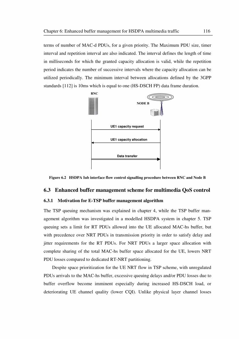
Chapter 6: Enhanced buffer management for HSDPA multimedia traffic 116
terms of number of MAC-d PDUs, for a given priority. The Maximum PDU size, timer
interval and repetition interval are also indicated. The interval defines the length of time
in milliseconds for which the granted capacity allocation is valid, while the repetition
period indicates the number of successive intervals where the capacity allocation can be
utilized periodically. The minimum interval between allocations defined by the 3GPP
standards [112] is 10ms which is equal to one (HS-DSCH FP) data frame duration.
UE1 capacity request
RNC
NODE B
UE1 capacity allocation
Data transfer
Figure 6.2 HSDPA Iub interface flow control signalling procedure between RNC and Node B
6.3 Enhanced buffer management scheme for multimedia QoS control
6.3.1 Motivation for E-TSP buffer management algorithm
The TSP queuing mechanism was explained in chapter 4, while the TSP buffer man-
agement algorithm was investigated in a modelled HSDPA system in chapter 5. TSP
queuing sets a limit for RT PDUs allowed into the UE allocated MAC-hs buffer, but
with precedence over NRT PDUs in transmission priority in order to satisfy delay and
jitter requirements for the RT PDUs. For NRT PDUs a larger space allocation with
complete sharing of the total MAC-hs buffer space allocated for the UE, lowers NRT
PDU losses compared to dedicated RT-NRT partitioning.
Despite space prioritization for the UE NRT flow in TSP scheme, with unregulated
PDUs arrivals to the MAC-hs buffer, excessive queuing delays and/or PDU losses due to
buffer overflow become imminent especially during increased HS-DSCH load, or
deteriorating UE channel quality (lower CQI). Unlike physical layer channel losses
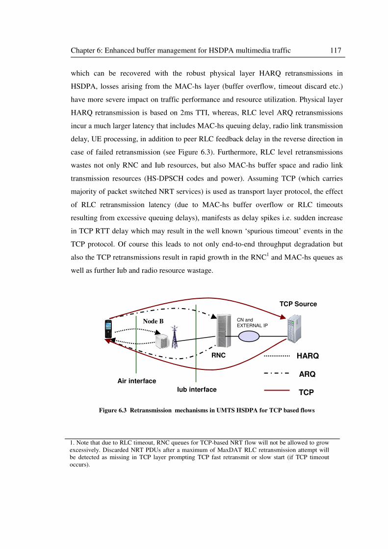
Chapter 6: Enhanced buffer management for HSDPA multimedia traffic 117
which can be recovered with the robust physical layer HARQ retransmissions in
HSDPA, losses arising from the MAC-hs layer (buffer overflow, timeout discard etc.)
have more severe impact on traffic performance and resource utilization. Physical layer
HARQ retransmission is based on 2ms TTI, whereas, RLC level ARQ retransmissions
incur a much larger latency that includes MAC-hs queuing delay, radio link transmission
delay, UE processing, in addition to peer RLC feedback delay in the reverse direction in
case of failed retransmission (see Figure 6.3). Furthermore, RLC level retransmissions
wastes not only RNC and Iub resources, but also MAC-hs buffer space and radio link
transmission resources (HS-DPSCH codes and power). Assuming TCP (which carries
majority of packet switched NRT services) is used as transport layer protocol, the effect
of RLC retransmission latency (due to MAC-hs buffer overflow or RLC timeouts
resulting from excessive queuing delays), manifests as delay spikes i.e. sudden increase
in TCP RTT delay which may result in the well known ‘spurious timeout’ events in the
TCP protocol. Of course this leads to not only end-to-end throughput degradation but
also the TCP retransmissions result in rapid growth in the RNC1 and MAC-hs queues as
well as further Iub and radio resource wastage.
HARQ
ARQ
TCPIub interface
Air interface
CN and EXTERNAL IP
TCP Source
RNC
Node B
Figure 6.3 Retransmission mechanisms in UMTS HSDPA for TCP based flows
1. Note that due to RLC timeout, RNC queues for TCP-based NRT flow will not be allowed to grow
excessively. Discarded NRT PDUs after a maximum of MaxDAT RLC retransmission attempt will
be detected as missing in TCP layer prompting TCP fast retransmit or slow start (if TCP timeout
occurs).
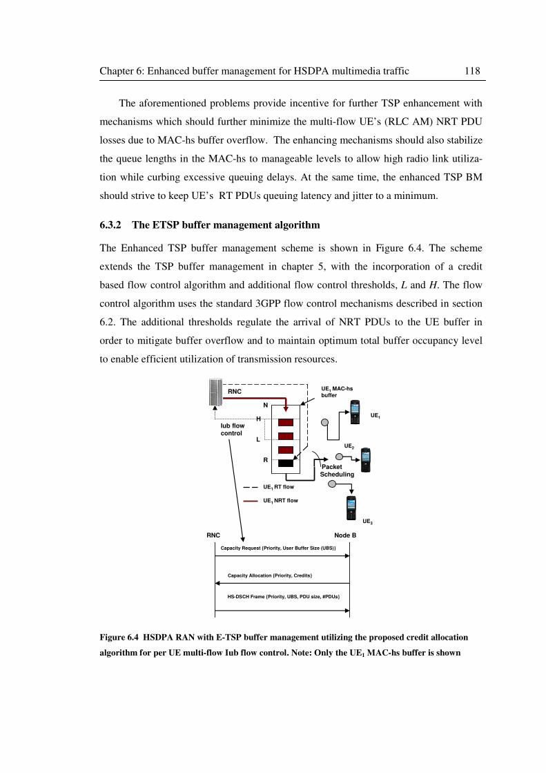
Chapter 6: Enhanced buffer management for HSDPA multimedia traffic 118
The aforementioned problems provide incentive for further TSP enhancement with
mechanisms which should further minimize the multi-flow UE’s (RLC AM) NRT PDU
losses due to MAC-hs buffer overflow. The enhancing mechanisms should also stabilize
the queue lengths in the MAC-hs to manageable levels to allow high radio link utiliza-
tion while curbing excessive queuing delays. At the same time, the enhanced TSP BM
should strive to keep UE’s RT PDUs queuing latency and jitter to a minimum.
6.3.2 The ETSP buffer management algorithm
The Enhanced TSP buffer management scheme is shown in Figure 6.4. The scheme
extends the TSP buffer management in chapter 5, with the incorporation of a credit
based flow control algorithm and additional flow control thresholds, L and H. The flow
control algorithm uses the standard 3GPP flow control mechanisms described in section
6.2. The additional thresholds regulate the arrival of NRT PDUs to the UE buffer in
order to mitigate buffer overflow and to maintain optimum total buffer occupancy level
to enable efficient utilization of transmission resources.
UE3
UE2
UE1 RT flow
UE1
UE1 MAC-hs
buffer
Capacity Request {Priority, User Buffer Size (UBS)}
RNC
UE1 NRT flow
R
H
L
N
Iub flow control
Packet Scheduling
Capacity Allocation {Priority, Credits}
HS-DSCH Frame {Priority, UBS, PDU size, #PDUs}
RNC Node B
Figure 6.4 HSDPA RAN with E-TSP buffer management utilizing the proposed credit allocation
algorithm for per UE multi-flow Iub flow control. Note: Only the UE1 MAC-hs buffer is shown
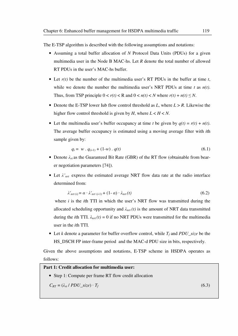
Chapter 6: Enhanced buffer management for HSDPA multimedia traffic 119
The E-TSP algorithm is described with the following assumptions and notations:
• Assuming a total buffer allocation of N Protocol Data Units (PDUs) for a given
multimedia user in the Node B MAC-hs. Let R denote the total number of allowed
RT PDUs in the user’s MAC-hs buffer.
• Let r(t) be the number of the multimedia user’s RT PDUs in the buffer at time t,
while we denote the number the multimedia user’s NRT PDUs at time t as n(t).
Thus, from TSP principle 0 < r(t) < R and 0 < n(t) < N where r(t) + n(t) ≤ N.
• Denote the E-TSP lower Iub flow control threshold as L, where L > R. Likewise the
higher flow control threshold is given by H, where L < H < N.
• Let the multimedia user’s buffer occupancy at time t be given by q(t) = r(t) + n(t).
The average buffer occupancy is estimated using a moving average filter with ith
sample given by:
qi = w . q(i-1) + (1-w) . q(t) (6.1)
• Denote λrt as the Guaranteed Bit Rate (GBR) of the RT flow (obtainable from bear-
er negotiation parameters [74]).
• Let λ’nrt express the estimated average NRT flow data rate at the radio interface
determined from:
λ'nrt (i) = α · λ'nrt (i-1) + (1- α) · λnrt (t) (6.2)
where i is the ith TTI in which the user’s NRT flow was transmitted during the
allocated scheduling opportunity and λnrt (t) is the amount of NRT data transmitted
during the ith TTI. λnrt (t) = 0 if no NRT PDUs were transmitted for the multimedia
user in the ith TTI.
• Let k denote a parameter for buffer overflow control, while Tf and PDU_size be the
HS_DSCH FP inter-frame period and the MAC-d PDU size in bits, respectively.
Given the above assumptions and notations, E-TSP scheme in HSDPA operates as
follows:
Part 1: Credit allocation for multimedia user:
• Step 1: Compute per frame RT flow credit allocation
CRT = (λrt / PDU_size) · Tf (6.3)
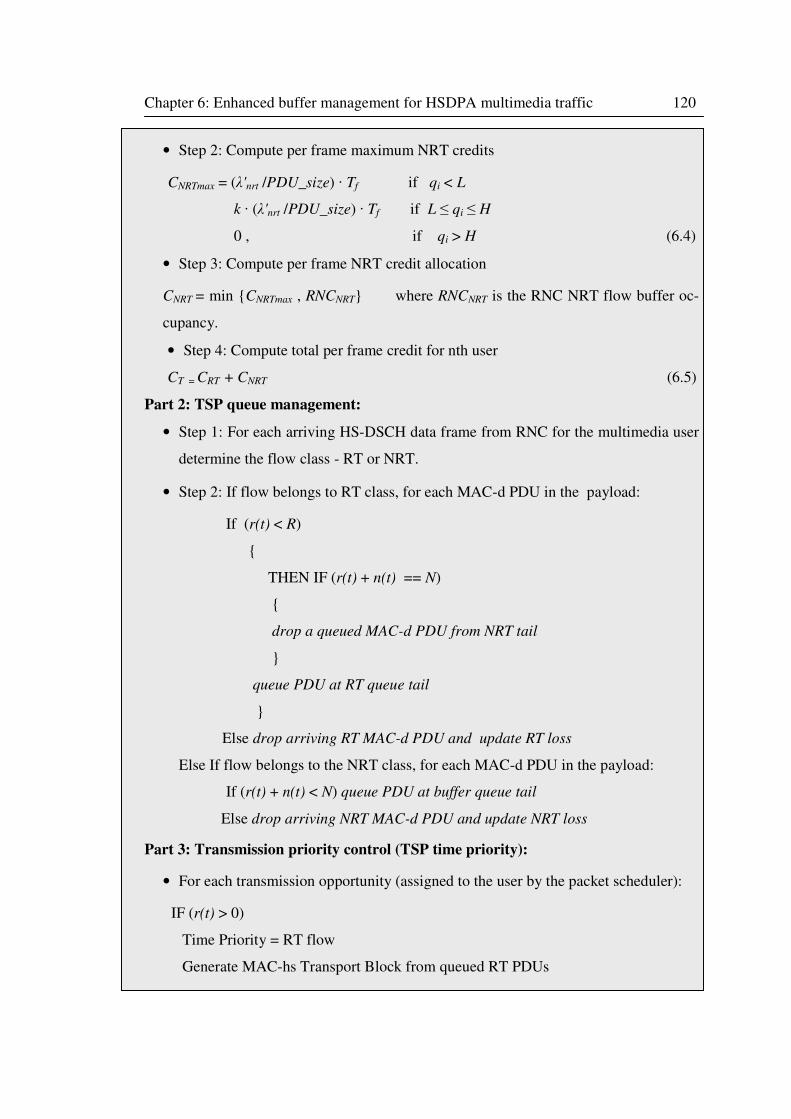
Chapter 6: Enhanced buffer management for HSDPA multimedia traffic 120
• Step 2: Compute per frame maximum NRT credits
CNRTmax = (λ'nrt /PDU_size) · Tf if qi < L
k · (λ'nrt /PDU_size) · Tf if L ≤ qi ≤ H
0 , if qi > H (6.4)
• Step 3: Compute per frame NRT credit allocation
CNRT = min {CNRTmax , RNCNRT} where RNCNRT is the RNC NRT flow buffer oc-
cupancy.
• Step 4: Compute total per frame credit for nth user
CT = CRT + CNRT (6.5)
Part 2: TSP queue management:
• Step 1: For each arriving HS-DSCH data frame from RNC for the multimedia user
determine the flow class - RT or NRT.
• Step 2: If flow belongs to RT class, for each MAC-d PDU in the payload:
If (r(t) < R)
{
THEN IF (r(t) + n(t) == N)
{
drop a queued MAC-d PDU from NRT tail
}
queue PDU at RT queue tail
}
Else drop arriving RT MAC-d PDU and update RT loss
Else If flow belongs to the NRT class, for each MAC-d PDU in the payload:
If (r(t) + n(t) < N) queue PDU at buffer queue tail
Else drop arriving NRT MAC-d PDU and update NRT loss
Part 3: Transmission priority control (TSP time priority):
• For each transmission opportunity (assigned to the user by the packet scheduler):
IF (r(t) > 0)
Time Priority = RT flow
Generate MAC-hs Transport Block from queued RT PDUs
Chapter 6: Enhanced buffer management for HSDPA multimedia traffic 121
ELSE IF (r(t) = =0 AND n(t) > 0)
Time Priority = NRT flow
Generate MAC-hs Transport Block from queued NRT PDUs
With the use of expression (6.2) in the credit allocation computation, NRT credit alloca-
tion and hence the NRT flow arrival rate for the multi-flow user, is made reactive to
channel load (via the inter-user packet scheduling algorithm), the user’s channel quality,
which is suited to the elastic nature of the NRT flow. Generally, better channel quality
(higher CQI) results in larger λ’nrt estimates, and hence, more credit allocation. The
opposite is true for poorer channel quality (low CQI). Similarly, with (6.4) the multi-
flow UE credit allocation is reactive to the UE MAC-hs total buffer occupancy level.
Since averages are used in the grant calculation, and because of possible time-lag
between issued credit and RNC reaction, the space between H and N absorbs instantane-
ous burst arrivals that could occur when CNRTmax = 0.
When the RT traffic being received in the UE multiple flow session is from a CBR
source (such as speech without silence suppression), expression (6.3) can be used to
grant a fixed credit allocation corresponding to the GBR metric in conjunction with a
large value of HS-DSCH Repetition Period in the Capacity Allocation frame. The same
technique can be employed when the RT flow in the UE session is VBR traffic, if it is
desired to introduce some form of traffic shaping; otherwise credit allocation for the
VBR RT flow should be computed thus:
CRT = max { (λrt / PDU_size) · Tf , UBSRT }
Where UBSRT is the number of RT PDUs in the RNC RLC queue, waiting for trans-
fer to the Node B MAC-hs over the Iub interface.
6.4 End-to-end simulation model and performance evaluation
This section is devoted to the performance evaluation of the proposed E-TSP BM
scheme described above. The main aim of the study is to investigate the potential end-to-
end QoS performance gains of the E-TSP buffer management scheme. Hence, simulation
was selected for the end-to-end performance evaluation rather than analytical modelling,
in order to include as much system detail as possible. The design of the simulator models
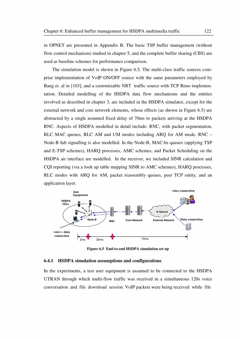
Chapter 6: Enhanced buffer management for HSDPA multimedia traffic 122
in OPNET are presented in Appendix B. The basic TSP buffer management (without
flow control mechanism) studied in chapter 5, and the complete buffer sharing (CBS) are
used as baseline schemes for performance comparison.
The simulation model is shown in Figure 6.5. The multi-class traffic sources com-
prise implementation of VoIP ON/OFF source with the same parameters employed by
Bang et. al in [103], and a customizable NRT traffic source with TCP Reno implemen-
tation. Detailed modelling of the HSDPA data flow mechanisms and the entities
involved as described in chapter 3, are included in the HSDPA simulator, except for the
external network and core network elements, whose effects (as shown in Figure 6.5) are
abstracted by a single assumed fixed delay of 70ms to packets arriving at the HSDPA
RNC. Aspects of HSDPA modelled in detail include: RNC, with packet segmentation,
RLC MAC queues, RLC AM and UM modes including ARQ for AM mode. RNC –
Node-B Iub signalling is also modelled. In the Node-B, MAC-hs queues (applying TSP
and E-TSP schemes), HARQ processes, AMC schemes, and Packet Scheduling on the
HSDPA air interface are modelled. In the receiver, we included SINR calculation and
CQI reporting (via a look up table mapping SINR to AMC schemes), HARQ processes,
RLC modes with ARQ for AM, packet reassembly queues, peer TCP entity, and an
application layer.
IP Network
User
Equipments
HSDPA
CELL
Node BRNC Core Network
voice connection
External Network
voice + data
connection
Data connection
70ms20ms2ms
Figure 6.5 End-to-end HSDPA simulation set up
6.4.1 HSDPA simulation assumptions and configurations
In the experiments, a test user equipment is assumed to be connected to the HSDPA
UTRAN through which multi-flow traffic was received in a simultaneous 120s voice
conversation and file download session. VoIP packets were being received while file
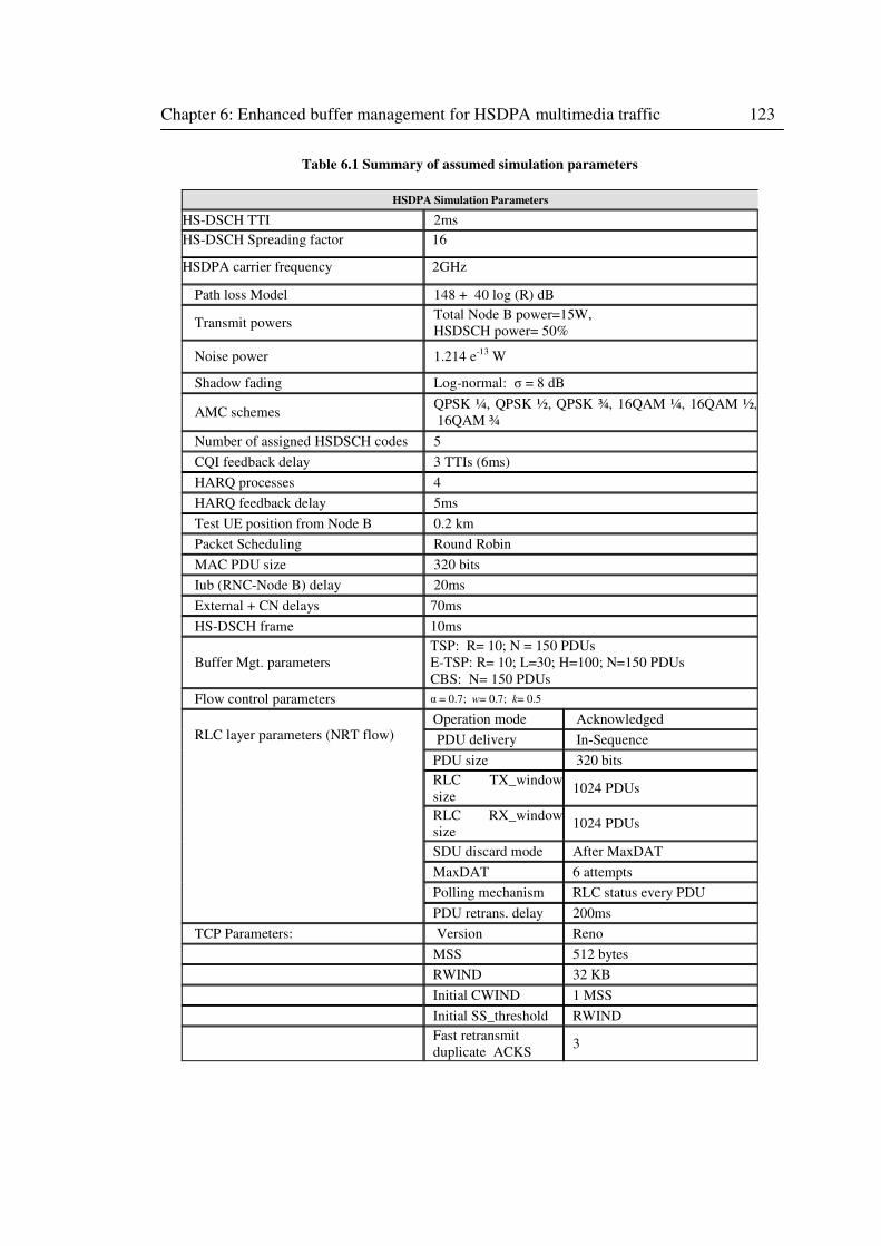
Chapter 6: Enhanced buffer management for HSDPA multimedia traffic 123
Table 6.1 Summary of assumed simulation parameters
HSDPA Simulation Parameters
HS-DSCH TTI 2ms
HS-DSCH Spreading factor 16
HSDPA carrier frequency 2GHz
Path loss Model 148 + 40 log (R) dB
Transmit powers Total Node B power=15W,
HSDSCH power= 50%
Noise power 1.214 e-13
W
Shadow fading Log-normal: σ = 8 dB
AMC schemes QPSK ¼, QPSK ½, QPSK ¾, 16QAM ¼, 16QAM ½,
16QAM ¾
Number of assigned HSDSCH codes 5
CQI feedback delay 3 TTIs (6ms)
HARQ processes 4
HARQ feedback delay 5ms
Test UE position from Node B 0.2 km
Packet Scheduling Round Robin
MAC PDU size 320 bits
Iub (RNC-Node B) delay 20ms
External + CN delays 70ms
HS-DSCH frame 10ms
Buffer Mgt. parameters
TSP: R= 10; N = 150 PDUs
E-TSP: R= 10; L=30; H=100; N=150 PDUs
CBS: N= 150 PDUs
Flow control parameters α = 0.7; w= 0.7; k= 0.5
RLC layer parameters (NRT flow) Operation mode Acknowledged
PDU delivery In-Sequence
PDU size 320 bits
RLC TX_window
size 1024 PDUs
RLC RX_window
size 1024 PDUs
SDU discard mode After MaxDAT
MaxDAT 6 attempts
Polling mechanism RLC status every PDU
PDU retrans. delay 200ms
TCP Parameters: Version Reno
MSS 512 bytes
RWIND 32 KB
Initial CWIND 1 MSS
Initial SS_threshold RWIND
Fast retransmit
duplicate ACKS 3
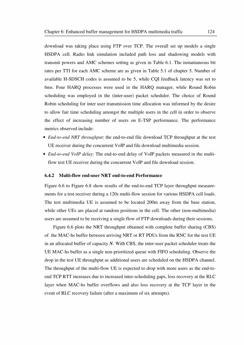
Chapter 6: Enhanced buffer management for HSDPA multimedia traffic 124
download was taking place using FTP over TCP. The overall set up models a single
HSDPA cell. Radio link simulation included path loss and shadowing models with
transmit powers and AMC schemes setting as given in Table 6.1. The instantaneous bit
rates per TTI for each AMC scheme are as given in Table 5.1 of chapter 5. Number of
available H-SDSCH codes is assumed to be 5, while CQI feedback latency was set to
6ms. Four HARQ processes were used in the HARQ manager, while Round Robin
scheduling was employed in the (inter-user) packet scheduler. The choice of Round
Robin scheduling for inter user transmission time allocation was informed by the desire
to allow fair time scheduling amongst the multiple users in the cell in order to observe
the effect of increasing number of users on E-TSP performance. The performance
metrics observed include:
• End-to-end NRT throughput: the end-to-end file download TCP throughput at the test
UE receiver during the concurrent VoIP and file download multimedia session.
• End-to-end VoIP delay: The end-to-end delay of VoIP packets measured in the multi-
flow test UE receiver during the concurrent VoIP and file download session.
6.4.2 Multi-flow end-user NRT end-to-end Performance
Figure 6.6 to Figure 6.8 show results of the end-to-end TCP layer throughput measure-
ments for a test receiver during a 120s multi-flow session for various HSDPA cell loads.
The test multimedia UE is assumed to be located 200m away from the base station,
while other UEs are placed at random positions in the cell. The other (non-multimedia)
users are assumed to be receiving a single flow of FTP downloads during their sessions.
Figure 6.6 plots the NRT throughput obtained with complete buffer sharing (CBS)
of the MAC-hs buffer between arriving NRT or RT PDUs from the RNC for the test UE
in an allocated buffer of capacity N. With CBS, the inter-user packet scheduler treats the
UE MAC-hs buffer as a single non-prioritized queue with FIFO scheduling. Observe the
drop in the test UE throughput as additional users are scheduled on the HSDPA channel.
The throughput of the multi-flow UE is expected to drop with more users as the end-to-
end TCP RTT increases due to increased inter-scheduling gaps, loss recovery at the RLC
layer when MAC-hs buffer overflows and also loss recovery at the TCP layer in the
event of RLC recovery failure (after a maximum of six attempts).
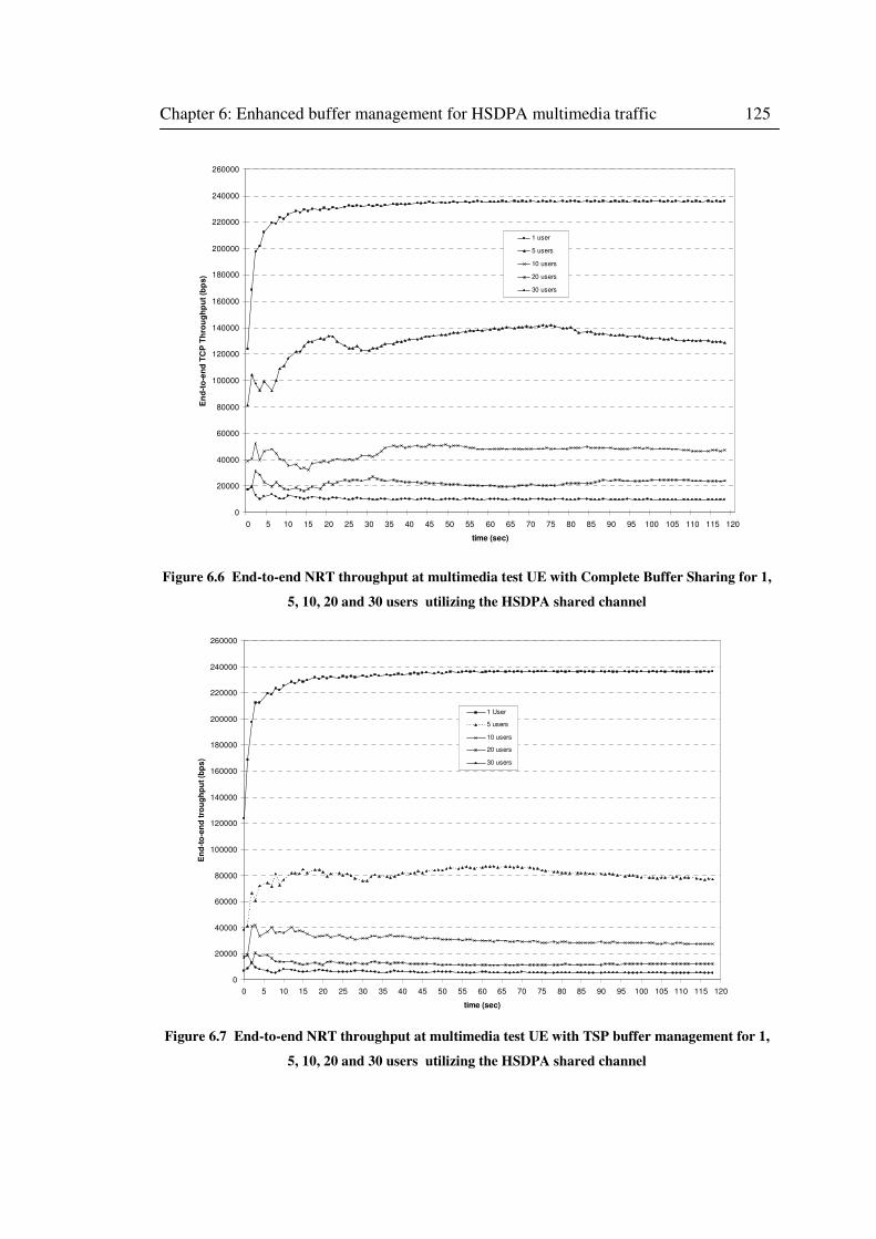
Chapter 6: Enhanced buffer management for HSDPA multimedia traffic 125
0
20000
40000
60000
80000
100000
120000
140000
160000
180000
200000
220000
240000
260000
0 5 10 15 20 25 30 35 40 45 50 55 60 65 70 75 80 85 90 95 100 105 110 115 120
time (sec)
En
d-t
o-e
nd
TC
P T
hro
ug
hp
ut
(bp
s)
1 user
5 users
10 users
20 users
30 users
Figure 6.6 End-to-end NRT throughput at multimedia test UE with Complete Buffer Sharing for 1,
5, 10, 20 and 30 users utilizing the HSDPA shared channel
0
20000
40000
60000
80000
100000
120000
140000
160000
180000
200000
220000
240000
260000
0 5 10 15 20 25 30 35 40 45 50 55 60 65 70 75 80 85 90 95 100 105 110 115 120
time (sec)
En
d-t
o-e
nd
tro
ug
hp
ut (b
ps
)
1 User
5 users
10 users
20 users
30 users
Figure 6.7 End-to-end NRT throughput at multimedia test UE with TSP buffer management for 1,
5, 10, 20 and 30 users utilizing the HSDPA shared channel
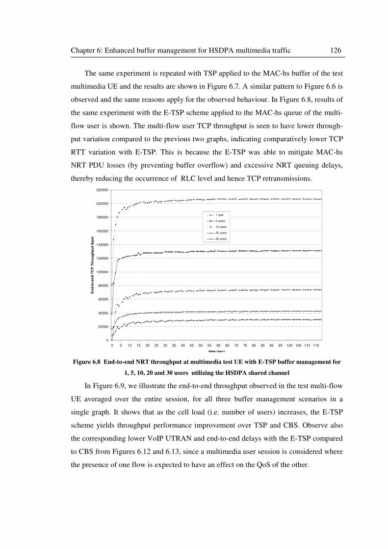
Chapter 6: Enhanced buffer management for HSDPA multimedia traffic 126
The same experiment is repeated with TSP applied to the MAC-hs buffer of the test
multimedia UE and the results are shown in Figure 6.7. A similar pattern to Figure 6.6 is
observed and the same reasons apply for the observed behaviour. In Figure 6.8, results of
the same experiment with the E-TSP scheme applied to the MAC-hs queue of the multi-
flow user is shown. The multi-flow user TCP throughput is seen to have lower through-
put variation compared to the previous two graphs, indicating comparatively lower TCP
RTT variation with E-TSP. This is because the E-TSP was able to mitigate MAC-hs
NRT PDU losses (by preventing buffer overflow) and excessive NRT queuing delays,
thereby reducing the occurrence of RLC level and hence TCP retransmissions.
0
20000
40000
60000
80000
100000
120000
140000
160000
180000
200000
220000
0 5 10 15 20 25 30 35 40 45 50 55 60 65 70 75 80 85 90 95 100 105 110 115
time (sec)
En
d-t
o-e
nd
TC
P T
hro
ug
hp
ut (b
ps)
1 user
5 users
10 users
20 users
30 users
Figure 6.8 End-to-end NRT throughput at multimedia test UE with E-TSP buffer management for
1, 5, 10, 20 and 30 users utilizing the HSDPA shared channel
In Figure 6.9, we illustrate the end-to-end throughput observed in the test multi-flow
UE averaged over the entire session, for all three buffer management scenarios in a
single graph. It shows that as the cell load (i.e. number of users) increases, the E-TSP
scheme yields throughput performance improvement over TSP and CBS. Observe also
the corresponding lower VoIP UTRAN and end-to-end delays with the E-TSP compared
to CBS from Figures 6.12 and 6.13, since a multimedia user session is considered where
the presence of one flow is expected to have an effect on the QoS of the other.
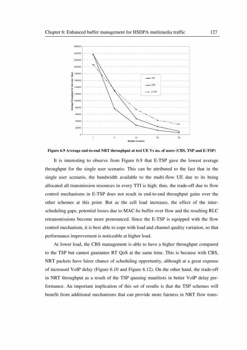
Chapter 6: Enhanced buffer management for HSDPA multimedia traffic 127
0
20000
40000
60000
80000
100000
120000
140000
160000
180000
200000
220000
240000
260000
1 5 10 20 30
Number of users
Av
era
ge
th
rou
gh
pu
t fo
r te
st
use
r (
bp
s)
TSP
CBS
E-TSP
Figure 6.9 Average end-to-end NRT throughput at test UE Vs no. of users (CBS, TSP and E-TSP)
It is interesting to observe from Figure 6.9 that E-TSP gave the lowest average
throughput for the single user scenario. This can be attributed to the fact that in the
single user scenario, the bandwidth available to the multi-flow UE due to its being
allocated all transmission resources in every TTI is high; thus, the trade-off due to flow
control mechanisms in E-TSP does not result in end-to-end throughput gains over the
other schemes at this point. But as the cell load increases, the effect of the inter-
scheduling gaps, potential losses due to MAC-hs buffer over flow and the resulting RLC
retransmissions become more pronounced. Since the E-TSP is equipped with the flow
control mechanism, it is best able to cope with load and channel quality variation, so that
performance improvement is noticeable at higher load.
At lower load, the CBS management is able to have a higher throughput compared
to the TSP but cannot guarantee RT QoS at the same time. This is because with CBS,
NRT packets have fairer chance of scheduling opportunity, although at a great expense
of increased VoIP delay (Figure 6.10 and Figure 6.12). On the other hand, the trade-off
in NRT throughput as a result of the TSP queuing manifests in better VoIP delay per-
formance. An important implication of this set of results is that the TSP schemes will
benefit from additional mechanisms that can provide more fairness in NRT flow trans-
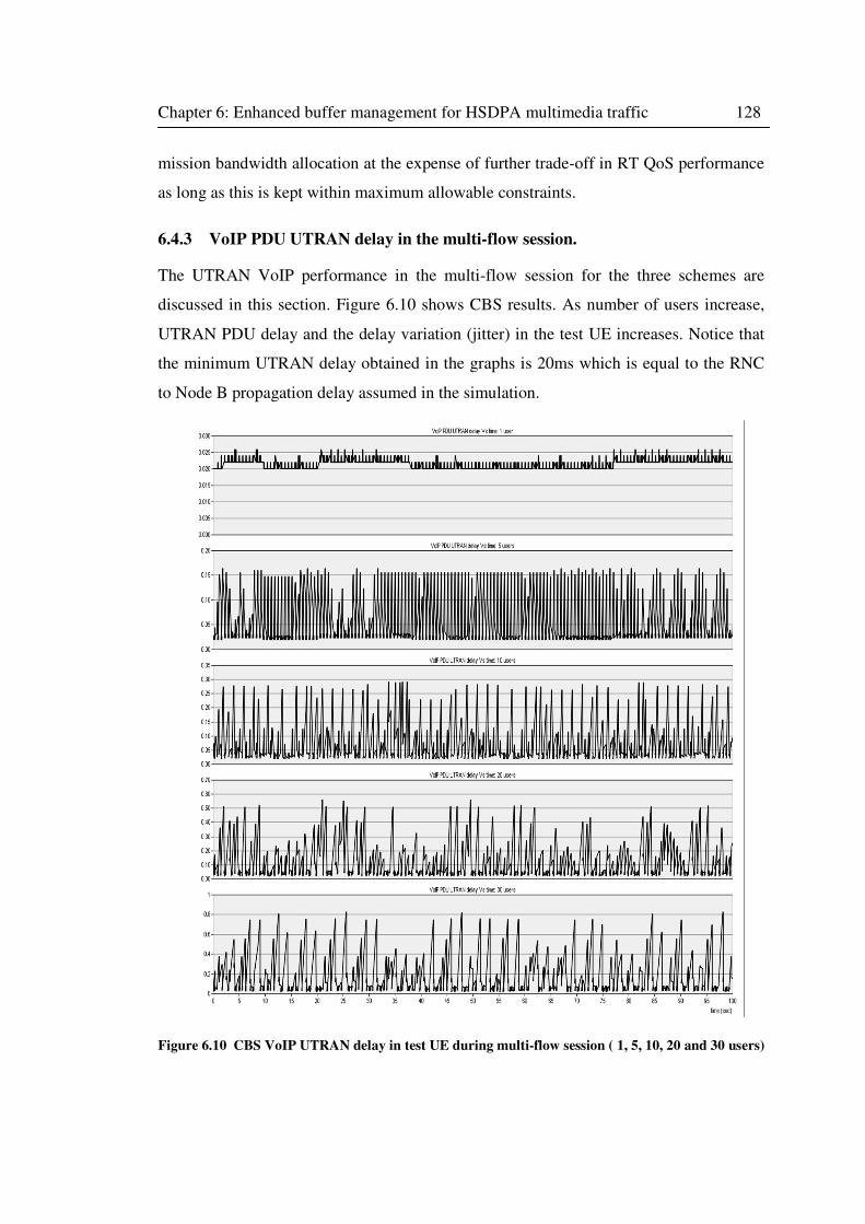
Chapter 6: Enhanced buffer management for HSDPA multimedia traffic 128
mission bandwidth allocation at the expense of further trade-off in RT QoS performance
as long as this is kept within maximum allowable constraints.
6.4.3 VoIP PDU UTRAN delay in the multi-flow session.
The UTRAN VoIP performance in the multi-flow session for the three schemes are
discussed in this section. Figure 6.10 shows CBS results. As number of users increase,
UTRAN PDU delay and the delay variation (jitter) in the test UE increases. Notice that
the minimum UTRAN delay obtained in the graphs is 20ms which is equal to the RNC
to Node B propagation delay assumed in the simulation.
Figure 6.10 CBS VoIP UTRAN delay in test UE during multi-flow session ( 1, 5, 10, 20 and 30 users)
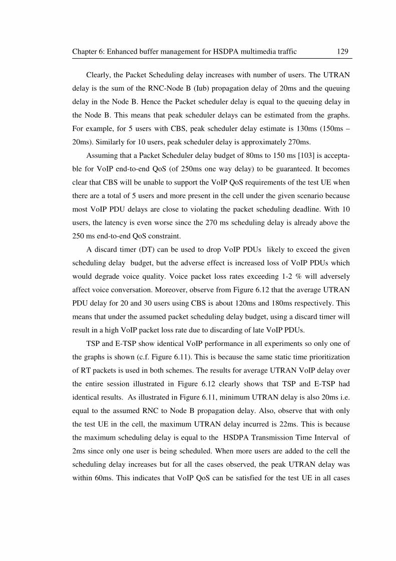
Chapter 6: Enhanced buffer management for HSDPA multimedia traffic 129
Clearly, the Packet Scheduling delay increases with number of users. The UTRAN
delay is the sum of the RNC-Node B (Iub) propagation delay of 20ms and the queuing
delay in the Node B. Hence the Packet scheduler delay is equal to the queuing delay in
the Node B. This means that peak scheduler delays can be estimated from the graphs.
For example, for 5 users with CBS, peak scheduler delay estimate is 130ms (150ms –
20ms). Similarly for 10 users, peak scheduler delay is approximately 270ms.
Assuming that a Packet Scheduler delay budget of 80ms to 150 ms [103] is accepta-
ble for VoIP end-to-end QoS (of 250ms one way delay) to be guaranteed. It becomes
clear that CBS will be unable to support the VoIP QoS requirements of the test UE when
there are a total of 5 users and more present in the cell under the given scenario because
most VoIP PDU delays are close to violating the packet scheduling deadline. With 10
users, the latency is even worse since the 270 ms scheduling delay is already above the
250 ms end-to-end QoS constraint.
A discard timer (DT) can be used to drop VoIP PDUs likely to exceed the given
scheduling delay budget, but the adverse effect is increased loss of VoIP PDUs which
would degrade voice quality. Voice packet loss rates exceeding 1-2 % will adversely
affect voice conversation. Moreover, observe from Figure 6.12 that the average UTRAN
PDU delay for 20 and 30 users using CBS is about 120ms and 180ms respectively. This
means that under the assumed packet scheduling delay budget, using a discard timer will
result in a high VoIP packet loss rate due to discarding of late VoIP PDUs.
TSP and E-TSP show identical VoIP performance in all experiments so only one of
the graphs is shown (c.f. Figure 6.11). This is because the same static time prioritization
of RT packets is used in both schemes. The results for average UTRAN VoIP delay over
the entire session illustrated in Figure 6.12 clearly shows that TSP and E-TSP had
identical results. As illustrated in Figure 6.11, minimum UTRAN delay is also 20ms i.e.
equal to the assumed RNC to Node B propagation delay. Also, observe that with only
the test UE in the cell, the maximum UTRAN delay incurred is 22ms. This is because
the maximum scheduling delay is equal to the HSDPA Transmission Time Interval of
2ms since only one user is being scheduled. When more users are added to the cell the
scheduling delay increases but for all the cases observed, the peak UTRAN delay was
within 60ms. This indicates that VoIP QoS can be satisfied for the test UE in all cases
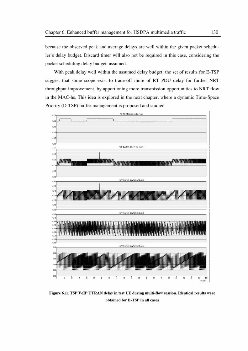
Chapter 6: Enhanced buffer management for HSDPA multimedia traffic 130
because the observed peak and average delays are well within the given packet schedu-
ler’s delay budget. Discard timer will also not be required in this case, considering the
packet scheduling delay budget assumed.
With peak delay well within the assumed delay budget, the set of results for E-TSP
suggest that some scope exist to trade-off more of RT PDU delay for further NRT
throughput improvement, by apportioning more transmission opportunities to NRT flow
in the MAC-hs. This idea is explored in the next chapter, where a dynamic Time-Space
Priority (D-TSP) buffer management is proposed and studied.
Figure 6.11 TSP VoIP UTRAN delay in test UE during multi-flow session. Identical results were
obtained for E-TSP in all cases
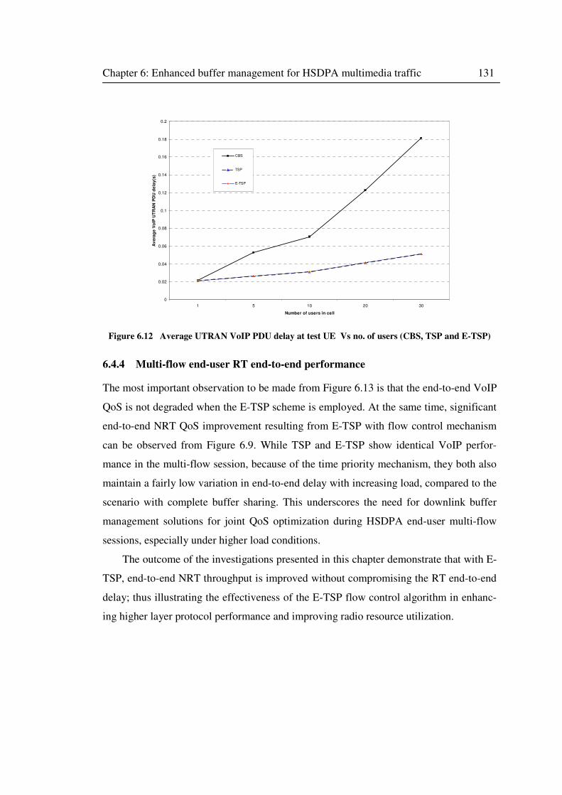
Chapter 6: Enhanced buffer management for HSDPA multimedia traffic 131
0
0.02
0.04
0.06
0.08
0.1
0.12
0.14
0.16
0.18
0.2
1 5 10 20 30
Number of users in cell
Av
era
ge
Vo
IP U
TR
AN
PD
U d
ela
y(s
)CBS
TSP
E-TSP
Figure 6.12 Average UTRAN VoIP PDU delay at test UE Vs no. of users (CBS, TSP and E-TSP)
6.4.4 Multi-flow end-user RT end-to-end performance
The most important observation to be made from Figure 6.13 is that the end-to-end VoIP
QoS is not degraded when the E-TSP scheme is employed. At the same time, significant
end-to-end NRT QoS improvement resulting from E-TSP with flow control mechanism
can be observed from Figure 6.9. While TSP and E-TSP show identical VoIP perfor-
mance in the multi-flow session, because of the time priority mechanism, they both also
maintain a fairly low variation in end-to-end delay with increasing load, compared to the
scenario with complete buffer sharing. This underscores the need for downlink buffer
management solutions for joint QoS optimization during HSDPA end-user multi-flow
sessions, especially under higher load conditions.
The outcome of the investigations presented in this chapter demonstrate that with E-
TSP, end-to-end NRT throughput is improved without compromising the RT end-to-end
delay; thus illustrating the effectiveness of the E-TSP flow control algorithm in enhanc-
ing higher layer protocol performance and improving radio resource utilization.
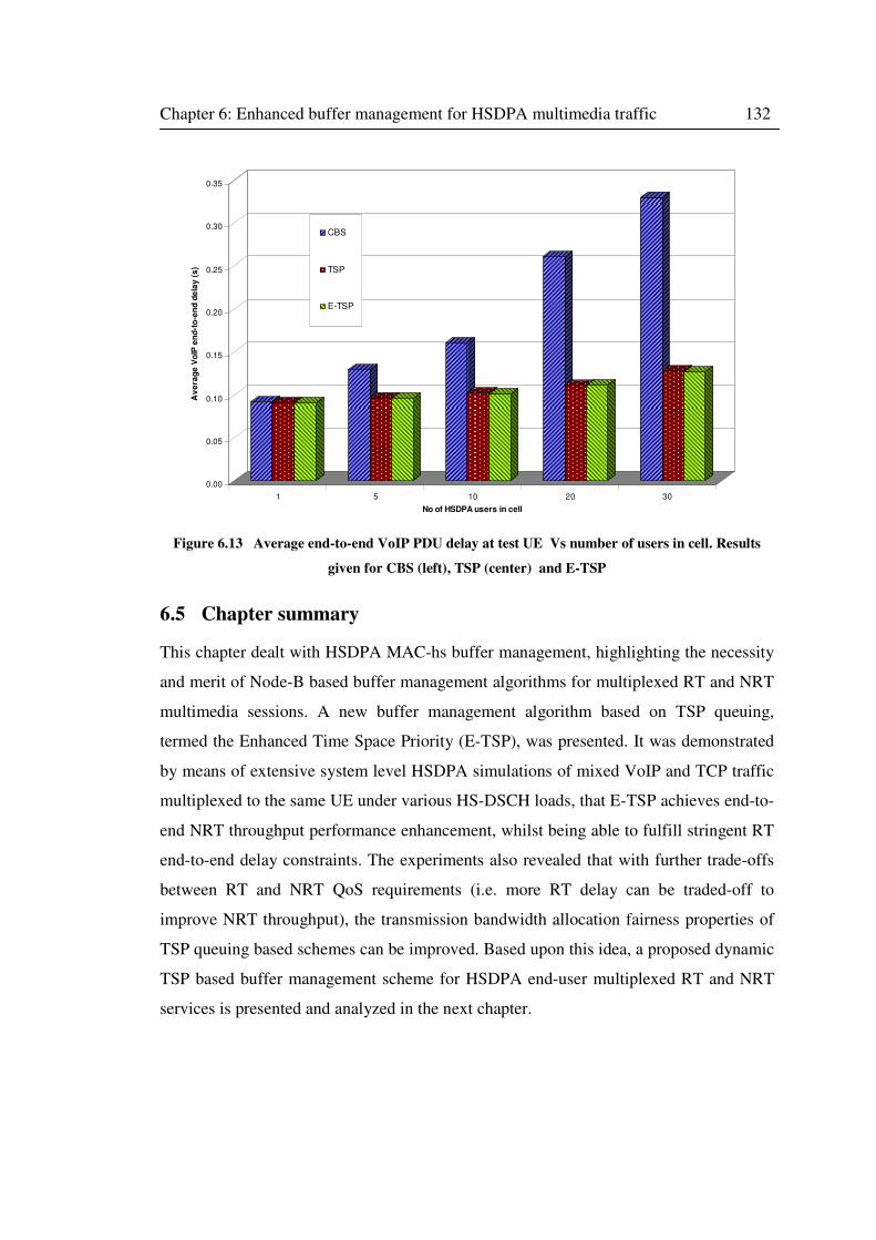
Chapter 6: Enhanced buffer management for HSDPA multimedia traffic 132
0.00
0.05
0.10
0.15
0.20
0.25
0.30
0.35
Av
era
ge
Vo
IP e
nd
-to
-en
d d
ela
y (
s)
1 5 10 20 30
No of HSDPA users in cell
CBS
TSP
E-TSP
Figure 6.13 Average end-to-end VoIP PDU delay at test UE Vs number of users in cell. Results
given for CBS (left), TSP (center) and E-TSP
6.5 Chapter summary
This chapter dealt with HSDPA MAC-hs buffer management, highlighting the necessity
and merit of Node-B based buffer management algorithms for multiplexed RT and NRT
multimedia sessions. A new buffer management algorithm based on TSP queuing,
termed the Enhanced Time Space Priority (E-TSP), was presented. It was demonstrated
by means of extensive system level HSDPA simulations of mixed VoIP and TCP traffic
multiplexed to the same UE under various HS-DSCH loads, that E-TSP achieves end-to-
end NRT throughput performance enhancement, whilst being able to fulfill stringent RT
end-to-end delay constraints. The experiments also revealed that with further trade-offs
between RT and NRT QoS requirements (i.e. more RT delay can be traded-off to
improve NRT throughput), the transmission bandwidth allocation fairness properties of
TSP queuing based schemes can be improved. Based upon this idea, a proposed dynamic
TSP based buffer management scheme for HSDPA end-user multiplexed RT and NRT
services is presented and analyzed in the next chapter.
133
Chapter 7
Dynamic Buffer Management for
HSDPA Multimedia Traffic
7.1 Introduction
As the demand for mobile multimedia and high speed data services continues to escalate,
end user multiplexed services support becomes even more crucial to current and next
generation mobile networks. In the previous chapter, E-TSP buffer management scheme
was proposed for HSDPA Node B as an end-to-end QoS enhancing solution for end user
multimedia traffic with diverse RT and NRT flows.
So far, TSP-based buffer management has been shown to be an effective and viable
solution for addressing MAC-hs priority handling of diverse flows scheduled/transmitted
to UEs with multiplexed services in the same session. Additionally, the studies underta-
ken in the previous chapter revealed further potential for enhancing (E-TSP) end-to-end
NRT throughput in the multi-flow session, by trading-off more of RT QoS for additional
NRT transmission bandwidth allocation. Thus, the concept of time (transmission)
priority switching is introduced to TSP/E-TSP to yield a dynamic time-space priority
buffer management scheme, D-TSP. D-TSP incorporates dynamic transmission priority
switching between the concurrent RT and NRT flows. This not only improves NRT
throughput, but also further alleviates potential NRT bandwidth starvation in the bottle-
neck air interface of the HSDPA system.
The main aim of this chapter is to present and analyze the proposed HSDPA D-TSP
buffer management algorithm. This chapter presents results of two sets of investigations.
Chapter 7: Dynamic buffer management for HSDPA multimedia traffic 134
The first, studies end-to-end performance of D-TSP on a simulated HSDPA system
under various cell loads, with a multiplexed session of simultaneous VoIP and TCP-
based FTP traffic. The second, investigates D-TSP end-to-end performance with con-
current real-time Constant Bit Rate (CBR) streaming and TCP-based FTP flows in the
multiplexed session, also under various HSDPA cell loads.
The rest of the chapter is organized as follows. Section 7.2 highlights motivations
for D-TSP and presents the algorithm. Section 7.3 presents the end-to-end evaluation
with multiplexed VoIP and TCP-based NRT traffic; while 7.4 studies D-TSP perfor-
mance with multiplexed RT CBR streaming and TCP-based NRT traffic. Concluding
remarks are given in the chapter summary in section 7.5.
7.2 Optimized QoS control of UE RT and NRT flows in HSDPA
This section examines some issues concerning the optimization of QoS performance of
concurrent RT and NRT flows in the multimedia session of the same HSDPA end user.
As mentioned before, RT and NRT classes of flows transmitted to the user, impose
conflicting QoS requirements which presents quite challenging buffer management
problem in terms of priority handling and joint QoS control. The previously proposed
BM schemes in this thesis, have been proven to provide effective solutions to these
problems. The main goal of the BM schemes is to guarantee RT class QoS by minimiz-
ing latency and jitter whilst also provisioning NRT class with minimized loss and
maximized throughput. However, the BM schemes can further optimize the QoS control
to increase the end-to-end NRT throughput at the expense of slightly reduced RT QoS
provisioning bounded by the minimum RT flow QoS requirements. Additional mechan-
isms are required in the BM schemes to achieve this, but the benefits for a system like
HSDPA, which are outlined below, far outweighs any potential drawbacks.
7.2.1 Incentives for optimized QoS control mechanisms in the TSP-based BM
schemes
By including QoS optimization mechanisms in the TSP BM schemes to further improve
NRT class throughput at the expense of slightly reduced RT class QoS, the following
benefits are foreseen in HSDPA:
Chapter 7: Dynamic buffer management for HSDPA multimedia traffic 135
• Since NRT class uses RLC Acknowledged Mode for MAC-d PDU transfer, RLC layer
performance improves dramatically due to reduced RLC round trip times and fewer
RLC retransmissions. Even a small percentage loss of NRT PDUs is detrimental. In
contrast, RT class uses RLC Unacknowledged Mode transfer where RT MAC PDU
losses have no effect on RLC RTT.
• Improved TCP performance and application response times: Unlike the RT flow which
will typically use UDP, the NRT flow in the HSDPA multimedia session utilizes TCP
as the transport layer protocol. TCP offers reliability and flow control for NRT services
and accounts for majority of data traffic in the Internet. TCP was originally designed
for wired networks, but extensive research efforts have concentrated on optimizing
TCP performance over wireless networks, including UMTS/HSDPA. Previous work
such as [113], [114], [115], [116], have shown that starvation of TCP-based NRT
flows in the lower layers have severe adverse effects on higher layer (RLC and TCP)
protocol performance. Boosting the TSP based BM with optimized QoS control me-
chanisms will alleviate potential starvation of the NRT class with consequent TCP
performance gains.
• Increased resource utilization efficiency: Loss of RT PDUs in the MAC-hs buffers
incur no additional RAN or radio resources. On the other hand, NRT PDUs lost due to
MAC-hs buffer overflow are retransmitted across all layers, thereby wasting network
and transmission resources from end to end.
• Reuse of existing QoS parameters and metrics: Existing 3GPP QoS parameters that are
known in the RNC and Node B (MAC-hs) and already used for other functionalities
such as Admission control, RAB allocation, packet scheduling etc. can be used as
input for QoS optimization mechanisms. Hence computational overhead will be mi-
nimal and architectural changes to 3GPP standards are not needed. Some already
existing 3GPP QoS parameters accessible to the MAC-hs include:
o GBR: Guaranteed bit rate
o DT: Discard timer
o SPI: Scheduling Priority Indicator
The proposed D-TSP buffer management algorithm can be considered an effective
mechanism for optimized RT and NRT QoS control in the UE multimedia session
Chapter 7: Dynamic buffer management for HSDPA multimedia traffic 136
because it allows for trade-off which ensures RT delay requirements are met whilst
maximizing NRT bandwidth allocation. Note that D-TSP can be used in conjunction
with the WGoS buffer optimization scheme proposed in Chapter 4, with WGoS provid-
ing a coarse optimization of the buffer threshold R, while D-TSP provides a finer
optimization of the QoS via transmission priority switching. Next, the D-TSP buffer
management algorithm is presented.
7.2.2 The Dynamic Time-Space Priority (D-TSP) buffer management scheme
The dynamic TSP buffer management scheme (D-TSP) extends the TSP and E-TSP
buffer management schemes by incorporating dynamic switching of transmission (time)
priority between the UE RT and NRT flows in the MAC-hs buffer. With TSP and E-TSP
BM, RT PDU transmission is always prioritized (static time prioritization). A possible
D-TSP priority switching mechanism is one based on (MAC-hs queuing) delay budget
(DB) estimates for the RT flow. Delay budget estimates are applied for example in [103]
to enable VoIP PDU bundling to improve HS-DSCH code utilization efficiency. DB can
be defined as a configurable parameter which could be set to a conservative value to
tighten the delay budget, or a higher value to relax the delay budget. For RT class flow
belonging to the conversational service such as VoIP flow, the maximum MAC-hs delay
budget can be estimated as:
DBmax =Y – (external network delays + CN delays + RNC delay + Iub delay) (7.1)
Where Y is the maximum allowable one way delay, assumed to be 250ms for voice
traffic [103]. If the RT flow class belongs to streaming service, then Y can be set to the
playout buffer size (in seconds) calculated from:
Y = Streaming buffer size (bits)/ playout rate (bits/sec) (7.2)
DBmax determines the Discard Timer (DT) setting. Recall that the discard timer is used to
discard MAC-d PDUs whose queuing delay in the MAC-hs has exceeded a given time.
The operating principle of the DTSP priority switching is that, for a given transmission
opportunity assigned by the MAC-hs Packet Scheduler, when the head-of-the-line RT
PDU queuing delay is unlikely to exceed the given delay budget, DB, transmission
priority is switched to the NRT flow. If the RT PDU head-of the-line delay is greater
than or equal to the delay budget or no NRT PDUs are present in the UE’s MAC-hs
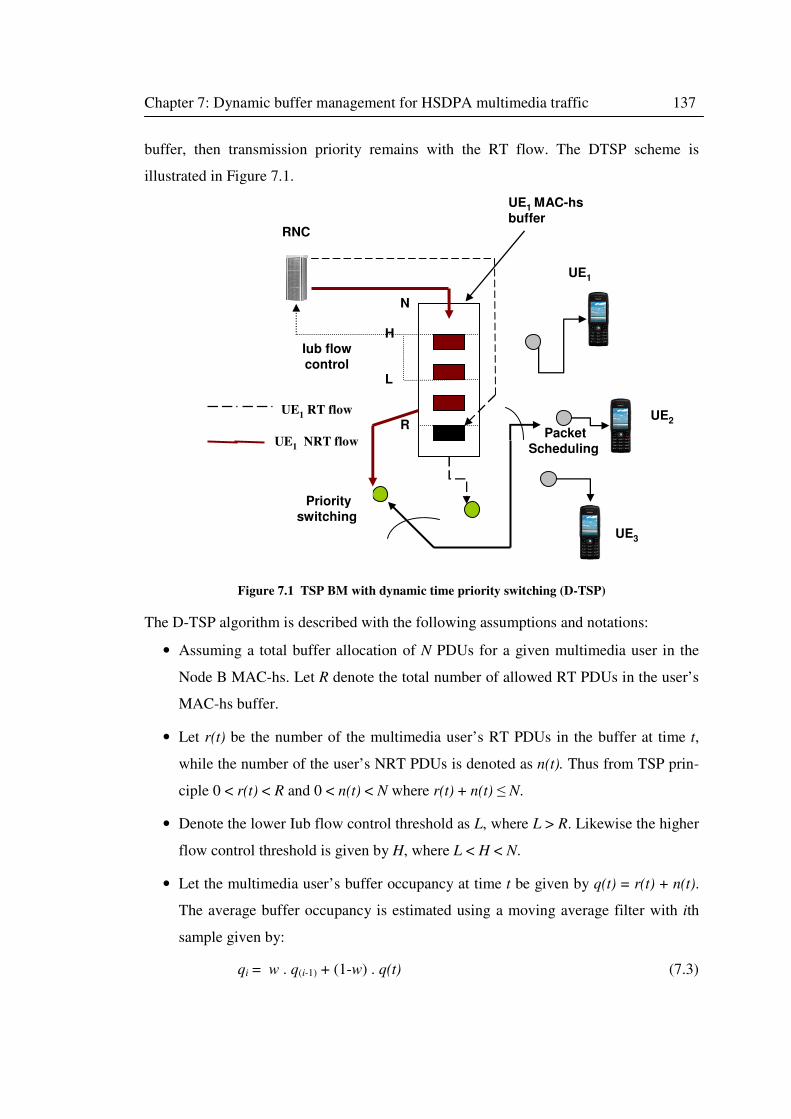
Chapter 7: Dynamic buffer management for HSDPA multimedia traffic 137
buffer, then transmission priority remains with the RT flow. The DTSP scheme is
illustrated in Figure 7.1.
RNC
UE1 NRT flow
R
H
L
N
Iub flow
control
Packet
Scheduling
Priority
switching
UE1 RT flow
UE1
UE1 MAC-hs
buffer
UE2
UE3
Figure 7.1 TSP BM with dynamic time priority switching (D-TSP)
The D-TSP algorithm is described with the following assumptions and notations:
• Assuming a total buffer allocation of N PDUs for a given multimedia user in the
Node B MAC-hs. Let R denote the total number of allowed RT PDUs in the user’s
MAC-hs buffer.
• Let r(t) be the number of the multimedia user’s RT PDUs in the buffer at time t,
while the number of the user’s NRT PDUs is denoted as n(t). Thus from TSP prin-
ciple 0 < r(t) < R and 0 < n(t) < N where r(t) + n(t) ≤ N.
• Denote the lower Iub flow control threshold as L, where L > R. Likewise the higher
flow control threshold is given by H, where L < H < N.
• Let the multimedia user’s buffer occupancy at time t be given by q(t) = r(t) + n(t).
The average buffer occupancy is estimated using a moving average filter with ith
sample given by:
qi = w . q(i-1) + (1-w) . q(t) (7.3)
Chapter 7: Dynamic buffer management for HSDPA multimedia traffic 138
• Denote λrt as the Guaranteed Bit Rate (GBR) of the RT flow (obtainable from bear-
er negotiation parameters [74]).
• Let λ’nrt express the estimated average NRT flow data rate at the radio interface
determined from:
λ'nrt (i) = α · λ'nrt (i-1) + (1- α) · λnrt (t) (7.4)
where i is the ith TTI in which the user’s NRT flow was transmitted during the
allocated scheduling opportunity and λnrt (t) is the amount of NRT data transmitted
during the ith TTI. λnrt (t) = 0 if no NRT PDUs were transmitted for the user in the
ith TTI.
• Let k denote a parameter for buffer overflow control, while Tf and PDU_size be the
HS_DSCH FP inter-frame period and the MAC-d PDU size in bits, respectively.
• A given delay budget, DB, for the UE RT flow PDU queuing in the Node B MAC-
hs is assumed. DB is used to determine the priority switching control parameter.
RT flow PDU inter-arrival time, i can be estimated from the already known GBR
thus:
i = PDU_size (bits)/ λrt (bits/sec) (7.5)
• Define a priority switching control parameter δ given by1:
δ = DB/ i (7.6)
• Assuming a discard timer (DT) [74] is used to discard MAC-d PDUs of the RT
flow with Node B MAC-hs queuing delay exceeding a given maximum delay
budget DBmax. If Y is the maximum allowable downlink delay then DBmax can be
estimated from equation (7.1).
• For each arriving RT MAC-d PDU for the multimedia user, DT is set to DBmax.
Thus any queued RT PDU is discarded (from the front of the queue), if it has been
in the MAC-hs buffer for up to DBmax time interval.
1. δ is expressed in PDU units. Equation (7.5) can be used to estimate RT interarrival times for a
CBR RT flow. For a VBR type flow, if the fixed credit allocation method in expression (7.7) is used
(providing some form of traffic shaping) then equation (7.5) can also be utilized with GBR =
GBRmin. Where GBRmin is the minimum guaranteed bit rate of the VBR flow.
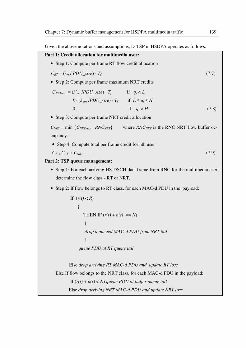
Chapter 7: Dynamic buffer management for HSDPA multimedia traffic 139
Given the above notations and assumptions, D-TSP in HSDPA operates as follows:
Part 1: Credit allocation for multimedia user:
• Step 1: Compute per frame RT flow credit allocation
CRT = (λrt / PDU_size) · Tf (7.7)
• Step 2: Compute per frame maximum NRT credits
CNRTmax = (λ'nrt /PDU_size) · Tf if qi < L
k · (λ'nrt /PDU_size) · Tf if L ≤ qi ≤ H
0 , if qi > H (7.8)
• Step 3: Compute per frame NRT credit allocation
CNRT = min {CNRTmax , RNCNRT} where RNCNRT is the RNC NRT flow buffer oc-
cupancy.
• Step 4: Compute total per frame credit for nth user
CT = CRT + CNRT (7.9)
Part 2: TSP queue management:
• Step 1: For each arriving HS-DSCH data frame from RNC for the multimedia user
determine the flow class - RT or NRT.
• Step 2: If flow belongs to RT class, for each MAC-d PDU in the payload:
If (r(t) < R)
{
THEN IF (r(t) + n(t) == N)
{
drop a queued MAC-d PDU from NRT tail
}
queue PDU at RT queue tail
}
Else drop arriving RT MAC-d PDU and update RT loss
Else If flow belongs to the NRT class, for each MAC-d PDU in the payload:
If (r(t) + n(t) < N) queue PDU at buffer queue tail
Else drop arriving NRT MAC-d PDU and update NRT loss
Chapter 7: Dynamic buffer management for HSDPA multimedia traffic 140
Part 3: Dynamic Transmission priority control:
• For each transmission opportunity (assigned to the user by the packet scheduler):
IF (r(t) < δ AND RT HOL delay < DBmax AND n(t) > 0)
Time Priority = NRT flow
Generate MAC-hs Transport Block from NRT PDUs
ELSE
Time Priority = RT flow
IF r(t)>0
Generate MAC-hs Transport Block from RT PDUs
Note that parts 1 and 2 of the DTSP buffer management algorithm are identical to
that of E-TSP. The difference lies in part 3, where D-TSP has dynamic time priority
switching in contrast to the static RT time prioritization policy of E-TSP (and TSP as
well).
7.3 D-TSP end-to-end performance evaluation I
In this section, the potential end-to-end QoS performance gains of the D-TSP BM
scheme are investigated using end-to-end HSDPA network simulations from the same
simulator developed for E-TSP investigation in the previous chapter. The design of the
simulator models are presented in Appendix B.
7.3.1 Simulation configuration and performance metrics
The experiments undertaken were designed to study the impact of dynamic priority
switching (using the proposed D-TSP BM strategy) on the UE RT and NRT flows’
performance. Hence, D-TSP BM was compared with E-TSP BM under the same traffic,
system and configuration parameters. The simulation set up consisted of a test multime-
dia user (UE1), assumed to be receiving simultaneous VoIP and FTP traffic over the HS-
DSCH during a 180s simulated voice conversation and file download session. VoIP
packets were being received while the file download was taking place using FTP over
TCP. The overall set up models a single HSDPA cell with Round Robin packet schedul-
ing to m users (as shown in the simulation set up in Figure 6.5 of chapter 6). A summary
of the HSDPA parameters used are given in Table 7.1.
Chapter 7: Dynamic buffer management for HSDPA multimedia traffic 141
The maximum allowable VoIP one way delay was taken as 250ms. Hence using eq-
uation (7.1), with Y = 250ms, assuming 70ms CN and external network delays, and 20ms
Iub delay, maximum MAC-hs delay budget DBmax = 160ms. This means that the discard
timer (DT) is also set to 160ms. The delay budget DB settings assumed in the experi-
ments were, 40ms, 80ms, 120ms and 160ms. The VoIP PDU inter-arrival time i is
computed from equation (7.5) assuming GBR is specified as 16kbps [74] and MAC
PDU size of 320 bits, yielding i = 20ms. Hence, the DTSP parameter δ corresponding to
the given delay budget DB settings were: 2, 4, 6, and 8 respectively as calculated from
equation (7.6).
The performance metrics observed during the experiments include:
• End-to-end NRT throughput: the end-to-end TCP throughput at the test multimedia
UE 1 during file download in the multi-flow session.
• RT PDU Discard Probability: defined as the number of late head-of-line RT PDUs
discarded from the (D-TSP or E-TSP) MAC-hs queue as a result of DT timeout.
• Percentage air interface utilization: calculated from Transport Block Size transmitted
divided by maximum Transport Block Size allowable by the selected AMC scheme,
measured at every transmission opportunity allocated to the UE.
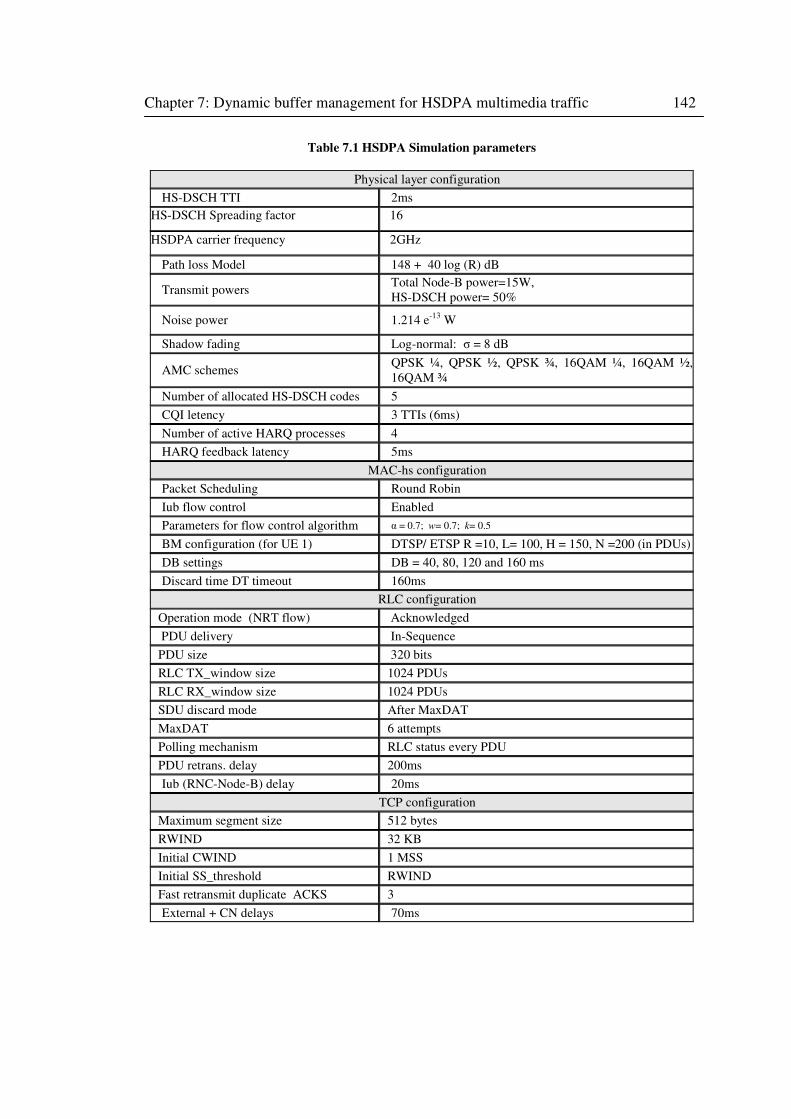
Chapter 7: Dynamic buffer management for HSDPA multimedia traffic 142
Table 7.1 HSDPA Simulation parameters
Physical layer configuration
HS-DSCH TTI 2ms
HS-DSCH Spreading factor 16
HSDPA carrier frequency 2GHz
Path loss Model 148 + 40 log (R) dB
Transmit powers Total Node-B power=15W,
HS-DSCH power= 50%
Noise power 1.214 e-13
W
Shadow fading Log-normal: σ = 8 dB
AMC schemes QPSK ¼, QPSK ½, QPSK ¾, 16QAM ¼, 16QAM ½,
16QAM ¾
Number of allocated HS-DSCH codes 5
CQI letency 3 TTIs (6ms)
Number of active HARQ processes 4
HARQ feedback latency 5ms
MAC-hs configuration
Packet Scheduling Round Robin
Iub flow control Enabled
Parameters for flow control algorithm α = 0.7; w= 0.7; k= 0.5
BM configuration (for UE 1) DTSP/ ETSP R =10, L= 100, H = 150, N =200 (in PDUs)
DB settings DB = 40, 80, 120 and 160 ms
Discard time DT timeout 160ms
RLC configuration
Operation mode (NRT flow) Acknowledged
PDU delivery In-Sequence
PDU size 320 bits
RLC TX_window size 1024 PDUs
RLC RX_window size 1024 PDUs
SDU discard mode After MaxDAT
MaxDAT 6 attempts
Polling mechanism RLC status every PDU
PDU retrans. delay 200ms
Iub (RNC-Node-B) delay 20ms
TCP configuration
Maximum segment size 512 bytes
RWIND 32 KB
Initial CWIND 1 MSS
Initial SS_threshold RWIND
Fast retransmit duplicate ACKS 3
External + CN delays 70ms
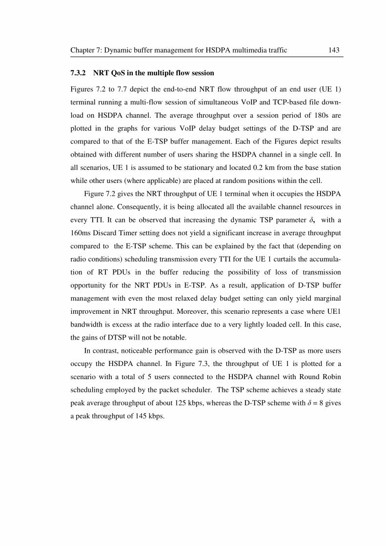
Chapter 7: Dynamic buffer management for HSDPA multimedia traffic 143
7.3.2 NRT QoS in the multiple flow session
Figures 7.2 to 7.7 depict the end-to-end NRT flow throughput of an end user (UE 1)
terminal running a multi-flow session of simultaneous VoIP and TCP-based file down-
load on HSDPA channel. The average throughput over a session period of 180s are
plotted in the graphs for various VoIP delay budget settings of the D-TSP and are
compared to that of the E-TSP buffer management. Each of the Figures depict results
obtained with different number of users sharing the HSDPA channel in a single cell. In
all scenarios, UE 1 is assumed to be stationary and located 0.2 km from the base station
while other users (where applicable) are placed at random positions within the cell.
Figure 7.2 gives the NRT throughput of UE 1 terminal when it occupies the HSDPA
channel alone. Consequently, it is being allocated all the available channel resources in
every TTI. It can be observed that increasing the dynamic TSP parameter δ, with a
160ms Discard Timer setting does not yield a significant increase in average throughput
compared to the E-TSP scheme. This can be explained by the fact that (depending on
radio conditions) scheduling transmission every TTI for the UE 1 curtails the accumula-
tion of RT PDUs in the buffer reducing the possibility of loss of transmission
opportunity for the NRT PDUs in E-TSP. As a result, application of D-TSP buffer
management with even the most relaxed delay budget setting can only yield marginal
improvement in NRT throughput. Moreover, this scenario represents a case where UE1
bandwidth is excess at the radio interface due to a very lightly loaded cell. In this case,
the gains of DTSP will not be notable.
In contrast, noticeable performance gain is observed with the D-TSP as more users
occupy the HSDPA channel. In Figure 7.3, the throughput of UE 1 is plotted for a
scenario with a total of 5 users connected to the HSDPA channel with Round Robin
scheduling employed by the packet scheduler. The TSP scheme achieves a steady state
peak average throughput of about 125 kbps, whereas the D-TSP scheme with δ = 8 gives
a peak throughput of 145 kbps.
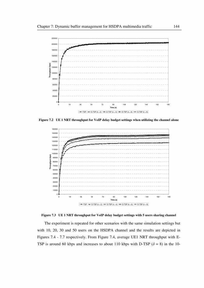
Chapter 7: Dynamic buffer management for HSDPA multimedia traffic 144
0
20000
40000
60000
80000
100000
120000
140000
160000
180000
200000
220000
0 18 36 54 72 90 108 126 144 162 180
Time (s)
Th
rou
gh
pu
t (b
ps
)
TSP D-TSP (k = 2) D-TSP (k = 4) D-TSP (k = 6) D-TSP (k = 8)
Figure 7.2 UE 1 NRT throughput for VoIP delay budget settings when utilizing the channel alone
0
10000
20000
30000
40000
50000
60000
70000
80000
90000
100000
110000
120000
130000
140000
150000
160000
0 18 36 54 72 90 108 126 144 162 180
Time (s)
Th
rou
gh
pu
t (b
ps
)
TSP D-TSP (k = 2) D-TSP (k = 4) D-TSP (k = 6) D-TSP (k = 8)
Figure 7.3 UE 1 NRT throughput for VoIP delay budget settings with 5 users sharing channel
The experiment is repeated for other scenarios with the same simulation settings but
with 10, 20, 30 and 50 users on the HSDPA channel and the results are depicted in
Figures 7.4 - 7.7 respectively. From Figure 7.4, average UE1 NRT throughput with E-
TSP is around 60 kbps and increases to about 110 kbps with D-TSP (δ = 8) in the 10-
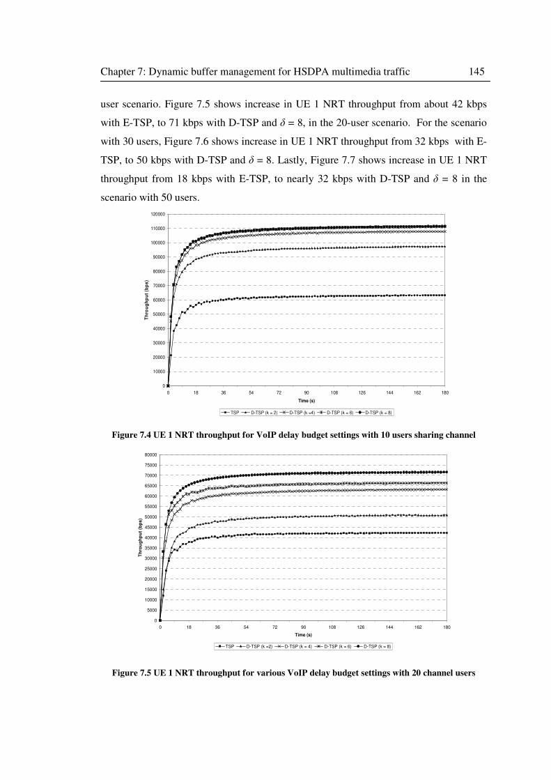
Chapter 7: Dynamic buffer management for HSDPA multimedia traffic 145
user scenario. Figure 7.5 shows increase in UE 1 NRT throughput from about 42 kbps
with E-TSP, to 71 kbps with D-TSP and δ = 8, in the 20-user scenario. For the scenario
with 30 users, Figure 7.6 shows increase in UE 1 NRT throughput from 32 kbps with E-
TSP, to 50 kbps with D-TSP and δ = 8. Lastly, Figure 7.7 shows increase in UE 1 NRT
throughput from 18 kbps with E-TSP, to nearly 32 kbps with D-TSP and δ = 8 in the
scenario with 50 users.
0
10000
20000
30000
40000
50000
60000
70000
80000
90000
100000
110000
120000
0 18 36 54 72 90 108 126 144 162 180
Time (s)
Th
rou
gh
pu
t (b
ps
)
TSP D-TSP (k = 2) D-TSP (k =4) D-TSP (k = 6) D-TSP (k = 8)
Figure 7.4 UE 1 NRT throughput for VoIP delay budget settings with 10 users sharing channel
0
5000
10000
15000
20000
25000
30000
35000
40000
45000
50000
55000
60000
65000
70000
75000
80000
0 18 36 54 72 90 108 126 144 162 180
Time (s)
Th
rou
gh
pu
t (b
ps
)
TSP D-TSP (k =2) D-TSP (k = 4) D-TSP (k = 6) D-TSP (k = 8)
Figure 7.5 UE 1 NRT throughput for various VoIP delay budget settings with 20 channel users
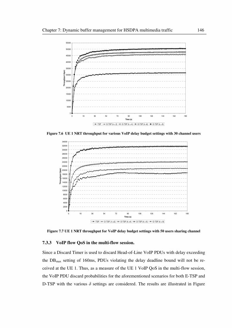
Chapter 7: Dynamic buffer management for HSDPA multimedia traffic 146
0
5000
10000
15000
20000
25000
30000
35000
40000
45000
50000
55000
0 18 36 54 72 90 108 126 144 162 180
Time (s)
Th
rou
gh
pu
t (b
ps
)
TSP D-TSP (k = 2) D-TSP (k = 4) D-TSP (k =6) D-TSP (k = 8)
Figure 7.6 UE 1 NRT throughput for various VoIP delay budget settings with 30 channel users
0
2000
4000
6000
8000
10000
12000
14000
16000
18000
20000
22000
24000
26000
28000
30000
32000
34000
0 18 36 54 72 90 108 126 144 162 180
Time (s)
Th
rou
gh
pu
t (b
ps
)
TSP D-TSP ( k =2) D-TSP (k =4) D-TSP (k = 6) D-TSP (k = 8)
Figure 7.7 UE 1 NRT throughput for VoIP delay budget settings with 50 users sharing channel
7.3.3 VoIP flow QoS in the multi-flow session.
Since a Discard Timer is used to discard Head-of-Line VoIP PDUs with delay exceeding
the DBmax setting of 160ms, PDUs violating the delay deadline bound will not be re-
ceived at the UE 1. Thus, as a measure of the UE 1 VoIP QoS in the multi-flow session,
the VoIP PDU discard probabilities for the aforementioned scenarios for both E-TSP and
D-TSP with the various δ settings are considered. The results are illustrated in Figure
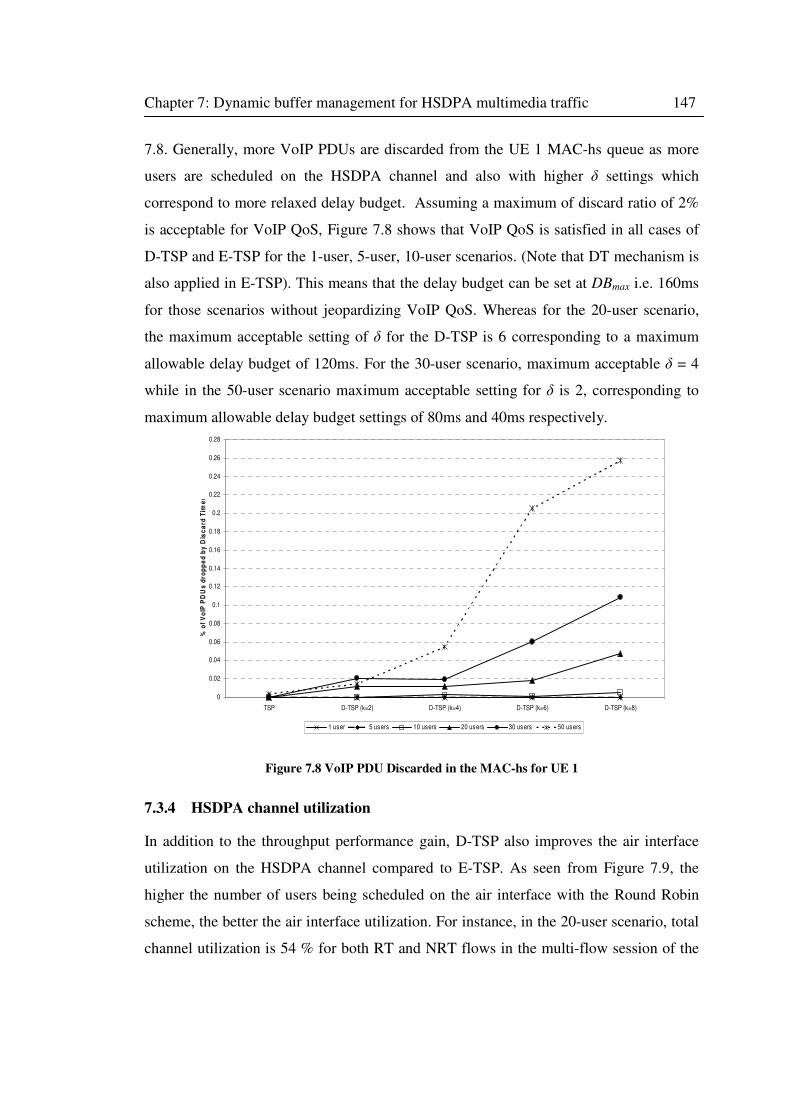
Chapter 7: Dynamic buffer management for HSDPA multimedia traffic 147
7.8. Generally, more VoIP PDUs are discarded from the UE 1 MAC-hs queue as more
users are scheduled on the HSDPA channel and also with higher δ settings which
correspond to more relaxed delay budget. Assuming a maximum of discard ratio of 2%
is acceptable for VoIP QoS, Figure 7.8 shows that VoIP QoS is satisfied in all cases of
D-TSP and E-TSP for the 1-user, 5-user, 10-user scenarios. (Note that DT mechanism is
also applied in E-TSP). This means that the delay budget can be set at DBmax i.e. 160ms
for those scenarios without jeopardizing VoIP QoS. Whereas for the 20-user scenario,
the maximum acceptable setting of δ for the D-TSP is 6 corresponding to a maximum
allowable delay budget of 120ms. For the 30-user scenario, maximum acceptable δ = 4
while in the 50-user scenario maximum acceptable setting for δ is 2, corresponding to
maximum allowable delay budget settings of 80ms and 40ms respectively.
0
0.02
0.04
0.06
0.08
0.1
0.12
0.14
0.16
0.18
0.2
0.22
0.24
0.26
0.28
TSP D-TSP (k=2) D-TSP (k=4) D-TSP (k=6) D-TSP (k=8)
% o
f V
oIP
PD
Us
dro
pp
ed
by
Dis
ca
rd T
ime
r
1 user 5 users 10 users 20 users 30 users 50 users
Figure 7.8 VoIP PDU Discarded in the MAC-hs for UE 1
7.3.4 HSDPA channel utilization
In addition to the throughput performance gain, D-TSP also improves the air interface
utilization on the HSDPA channel compared to E-TSP. As seen from Figure 7.9, the
higher the number of users being scheduled on the air interface with the Round Robin
scheme, the better the air interface utilization. For instance, in the 20-user scenario, total
channel utilization is 54 % for both RT and NRT flows in the multi-flow session of the
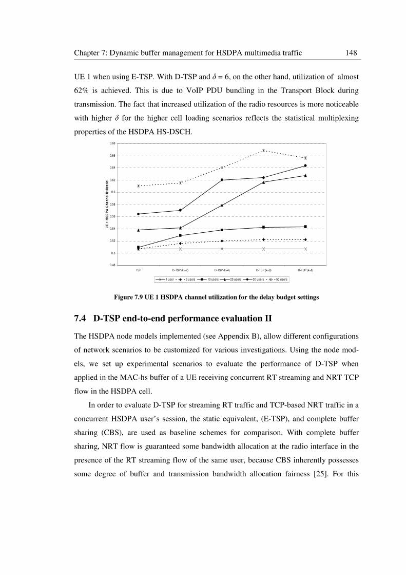
Chapter 7: Dynamic buffer management for HSDPA multimedia traffic 148
UE 1 when using E-TSP. With D-TSP and δ = 6, on the other hand, utilization of almost
62% is achieved. This is due to VoIP PDU bundling in the Transport Block during
transmission. The fact that increased utilization of the radio resources is more noticeable
with higher δ for the higher cell loading scenarios reflects the statistical multiplexing
properties of the HSDPA HS-DSCH.
0.48
0.5
0.52
0.54
0.56
0.58
0.6
0.62
0.64
0.66
0.68
TSP D-TSP (k =2) D-TSP (k=4) D-TSP (k=6) D-TSP (k=8)
UE
1 H
SD
PA
Ch
an
ne
l U
tili
za
tio
n
1 user 5 users 10 users 20 users 30 users 50 users
Figure 7.9 UE 1 HSDPA channel utilization for the delay budget settings
7.4 D-TSP end-to-end performance evaluation II
The HSDPA node models implemented (see Appendix B), allow different configurations
of network scenarios to be customized for various investigations. Using the node mod-
els, we set up experimental scenarios to evaluate the performance of D-TSP when
applied in the MAC-hs buffer of a UE receiving concurrent RT streaming and NRT TCP
flow in the HSDPA cell.
In order to evaluate D-TSP for streaming RT traffic and TCP-based NRT traffic in a
concurrent HSDPA user’s session, the static equivalent, (E-TSP), and complete buffer
sharing (CBS), are used as baseline schemes for comparison. With complete buffer
sharing, NRT flow is guaranteed some bandwidth allocation at the radio interface in the
presence of the RT streaming flow of the same user, because CBS inherently possesses
some degree of buffer and transmission bandwidth allocation fairness [25]. For this
Chapter 7: Dynamic buffer management for HSDPA multimedia traffic 149
reason, CBS provides a comparative baseline scheme to evaluate the NRT flow starva-
tion mitigation capabilities of D-TSP.
Recall that D-TSP adds dynamic priority switching to TSP/E-TSP in order to pri-
oritize NRT transmission while RT flow delay is kept within a given delay budget.
Hence, with D-TSP, NRT flow performance is expected to improve, but RT streaming
being a ‘greedy source’ traffic has the potential to cause NRT bandwidth starvation. So
the study is aimed at investigating the impact of RT streaming flow on the concurrent
NRT TCP flow and the effectiveness of D-TSP in mitigating NRT flow starvation while
still ensuring RT streaming QoS requirements are not violated.
In the experiments, a test user equipment (UE1) is connected to the UTRAN and
configured to receive multi-flow traffic of simultaneous RT streaming and NRT file
download. The RT stream is 64 kbps Constant Bit Rate (CBR) encoded video, while the
NRT stream is from a TCP based file download. The overall set up models a single
HSDPA cell with Round Robin scheduling to m users. A summary of the simulation
parameters are as given in Table 6.1 but with D-TSP/E-TSP parameters replaced by the
following values: R = 32, L= 72, H = 144, N =192. Where applicable as a comparative
scheme, the complete buffer sharing parameter used is N=192, i.e. total buffer capacity.
7.4.1 Buffer dimensioning
Assuming a downlink maximum transfer delay of 250ms, the maximum MAC-hs delay
budget DBmax can be calculated from equation (7.1), given that assumed CN + external
delay + Iub delay sum up to 90ms (see Table 6.1). It is reasonable to assume that RNC
queuing contributes very little delay comparatively because the D-TSP (and E-TSP) flow
control algorithm design ensures that RT PDUs are not held back in the RNC queues.
Moreover, this was confirmed during the simulations. Thus, from equation (7.1) DBmax
= 160ms, and, therefore RT discard timer DT is set to 160ms.
For the 64 kbps CBR RT stream, λrt = 64 kbps hence:
R = (λrt * DBmax) /PDU_size = 32 PDUs
Likewise, assuming a maximum bit rate of 256 kbps for NRT flow and maximum
average MAC-hs delay budget of 200ms:
Buffer size = (256 000 * 0.2)/PDU_size = 160.
Chapter 7: Dynamic buffer management for HSDPA multimedia traffic 150
Hence, a total buffer size N = 32 +160 = 192 PDUs in the MAC-hs is taken for the UE.
For the flow control thresholds, H= 0.75* N = 144, and L =0.5 * H = 72, are assumed.
7.4.2 Performance metrics
In the experiments, we consider MAC-hs queuing delay budgets, DB, of 40, 80, 120 and
160 ms which from equation (7.6), correspond to δ = 8, 16, 24 and 32 respectively. Note
that the discard timer, DT discards RT streaming packets whose MAC-hs queuing delay
≥ 160ms from the head of the D-TSP queue. The performance metrics observed are:
• Average end-to-end NRT throughput: The time average of the throughput of the
TCP-based flow measured in the test of the UE..
• RT PDU discard ratio: The ratio of late RT streaming PDUs discarded in the
MAC-hs as a result of DT timeout.
• RT inter-packet playout delay: The playout delay between successive packets of
the RT streaming flow queued in the UE playout buffer after the first initial buffer-
ing delay of DBmax.
Several scenarios with different HSDPA cell loads were considered i.e. m = 1, 5, 10, 20
and 30 users simultaneously active during the test UE’s concurrent streaming and file
download session of 120s duration.
7.4.3 End-to-end NRT throughput evaluation
Figure 7.10 plots the average end-to-end NRT flow throughput of an HSDPA end user
(UE1) terminal running a session of simultaneous CBR 64 Kbps RT video streaming and
TCP-based file download. The average throughput is plotted against the number of users
sharing the HSDPA channel in a single cell with Round Robin packet scheduling. The
time average of the obtained throughput measured in the UE over a session period of
120s for δ = 8, 16, 24 and 32 delay budget settings are compared to that of E-TSP and
the CBS buffer management. In all the scenarios UE1 is assumed to be located at 0.2 km
from the base station and moving away at 3 km/h, while other users are placed at random
positions in the cell. From Figure 7.10, it can be seen that in the single user scenario i.e.
when UE1 occupies the channel alone, the D-TSP scheme in all DB settings give only
slightly better throughput than TSP or CBS. This represents a lightly loaded HSDPA
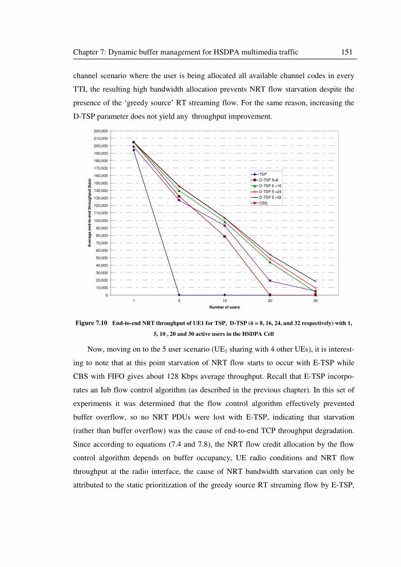
Chapter 7: Dynamic buffer management for HSDPA multimedia traffic 151
channel scenario where the user is being allocated all available channel codes in every
TTI, the resulting high bandwidth allocation prevents NRT flow starvation despite the
presence of the ‘greedy source’ RT streaming flow. For the same reason, increasing the
D-TSP parameter does not yield any throughput improvement.
0
10,000
20,000
30,000
40,000
50,000
60,000
70,000
80,000
90,000
100,000
110,000
120,000
130,000
140,000
150,000
160,000
170,000
180,000
190,000
200,000
210,000
220,000
1 5 10 20 30
Number of users
Ave
rag
e e
nd
-to
-en
d t
hro
ug
hp
ut (b
ps)
TSP
D-TSP δ=8
D-TSP δ =16
D-TSP δ =24
D-TSP δ =32
CBS
Figure 7.10 End-to-end NRT throughput of UE1 for TSP, D-TSP (δ = 8, 16, 24, and 32 respectively) with 1,
5, 10 , 20 and 30 active users in the HSDPA Cell
Now, moving on to the 5 user scenario (UE1 sharing with 4 other UEs), it is interest-
ing to note that at this point starvation of NRT flow starts to occur with E-TSP while
CBS with FIFO gives about 128 Kbps average throughput. Recall that E-TSP incorpo-
rates an Iub flow control algorithm (as described in the previous chapter). In this set of
experiments it was determined that the flow control algorithm effectively prevented
buffer overflow, so no NRT PDUs were lost with E-TSP, indicating that starvation
(rather than buffer overflow) was the cause of end-to-end TCP throughput degradation.
Since according to equations (7.4 and 7.8), the NRT flow credit allocation by the flow
control algorithm depends on buffer occupancy, UE radio conditions and NRT flow
throughput at the radio interface, the cause of NRT bandwidth starvation can only be
attributed to the static prioritization of the greedy source RT streaming flow by E-TSP,
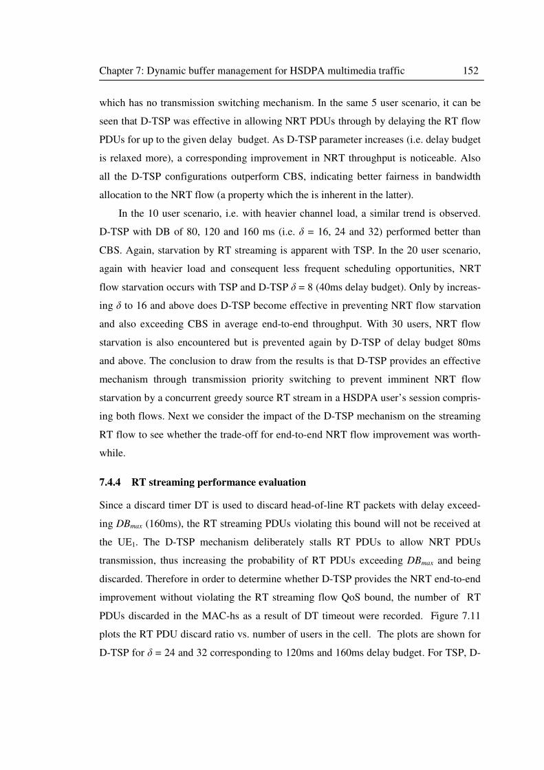
Chapter 7: Dynamic buffer management for HSDPA multimedia traffic 152
which has no transmission switching mechanism. In the same 5 user scenario, it can be
seen that D-TSP was effective in allowing NRT PDUs through by delaying the RT flow
PDUs for up to the given delay budget. As D-TSP parameter increases (i.e. delay budget
is relaxed more), a corresponding improvement in NRT throughput is noticeable. Also
all the D-TSP configurations outperform CBS, indicating better fairness in bandwidth
allocation to the NRT flow (a property which the is inherent in the latter).
In the 10 user scenario, i.e. with heavier channel load, a similar trend is observed.
D-TSP with DB of 80, 120 and 160 ms (i.e. δ = 16, 24 and 32) performed better than
CBS. Again, starvation by RT streaming is apparent with TSP. In the 20 user scenario,
again with heavier load and consequent less frequent scheduling opportunities, NRT
flow starvation occurs with TSP and D-TSP δ = 8 (40ms delay budget). Only by increas-
ing δ to 16 and above does D-TSP become effective in preventing NRT flow starvation
and also exceeding CBS in average end-to-end throughput. With 30 users, NRT flow
starvation is also encountered but is prevented again by D-TSP of delay budget 80ms
and above. The conclusion to draw from the results is that D-TSP provides an effective
mechanism through transmission priority switching to prevent imminent NRT flow
starvation by a concurrent greedy source RT stream in a HSDPA user’s session compris-
ing both flows. Next we consider the impact of the D-TSP mechanism on the streaming
RT flow to see whether the trade-off for end-to-end NRT flow improvement was worth-
while.
7.4.4 RT streaming performance evaluation
Since a discard timer DT is used to discard head-of-line RT packets with delay exceed-
ing DBmax (160ms), the RT streaming PDUs violating this bound will not be received at
the UE1. The D-TSP mechanism deliberately stalls RT PDUs to allow NRT PDUs
transmission, thus increasing the probability of RT PDUs exceeding DBmax and being
discarded. Therefore in order to determine whether D-TSP provides the NRT end-to-end
improvement without violating the RT streaming flow QoS bound, the number of RT
PDUs discarded in the MAC-hs as a result of DT timeout were recorded. Figure 7.11
plots the RT PDU discard ratio vs. number of users in the cell. The plots are shown for
D-TSP for δ = 24 and 32 corresponding to 120ms and 160ms delay budget. For TSP, D-
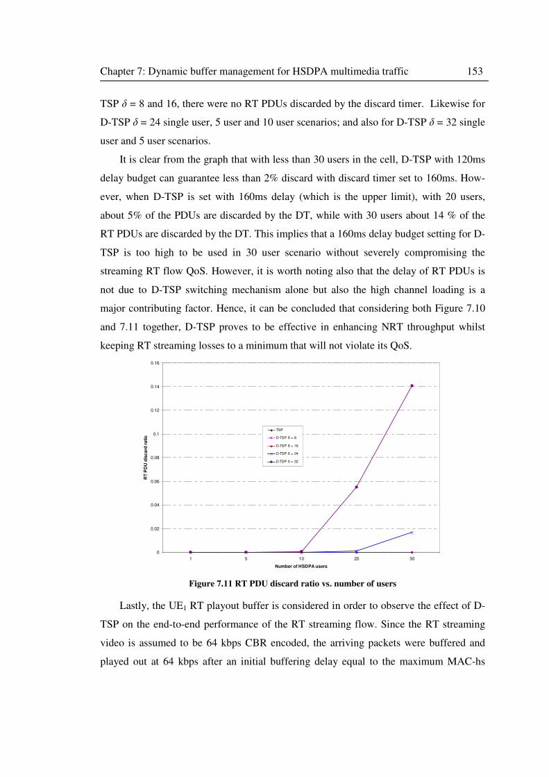
Chapter 7: Dynamic buffer management for HSDPA multimedia traffic 153
TSP δ = 8 and 16, there were no RT PDUs discarded by the discard timer. Likewise for
D-TSP δ = 24 single user, 5 user and 10 user scenarios; and also for D-TSP δ = 32 single
user and 5 user scenarios.
It is clear from the graph that with less than 30 users in the cell, D-TSP with 120ms
delay budget can guarantee less than 2% discard with discard timer set to 160ms. How-
ever, when D-TSP is set with 160ms delay (which is the upper limit), with 20 users,
about 5% of the PDUs are discarded by the DT, while with 30 users about 14 % of the
RT PDUs are discarded by the DT. This implies that a 160ms delay budget setting for D-
TSP is too high to be used in 30 user scenario without severely compromising the
streaming RT flow QoS. However, it is worth noting also that the delay of RT PDUs is
not due to D-TSP switching mechanism alone but also the high channel loading is a
major contributing factor. Hence, it can be concluded that considering both Figure 7.10
and 7.11 together, D-TSP proves to be effective in enhancing NRT throughput whilst
keeping RT streaming losses to a minimum that will not violate its QoS.
0
0.02
0.04
0.06
0.08
0.1
0.12
0.14
0.16
1 5 10 20 30
Number of HSDPA users
RT
PD
U d
isc
ard
ra
tio
TSP
D-TSP δ = 8
D-TSP δ = 16
D-TSP δ = 24
D-TSP δ = 32
Figure 7.11 RT PDU discard ratio vs. number of users
Lastly, the UE1 RT playout buffer is considered in order to observe the effect of D-
TSP on the end-to-end performance of the RT streaming flow. Since the RT streaming
video is assumed to be 64 kbps CBR encoded, the arriving packets were buffered and
played out at 64 kbps after an initial buffering delay equal to the maximum MAC-hs
Chapter 7: Dynamic buffer management for HSDPA multimedia traffic 154
delay budget DBmax of 160ms. The inter-packet playout delay i.e. the delay between each
successive packet played out from the buffer was measured. A constant delay is ex-
pected if the buffer always contains a packet for playout, otherwise if the buffer empties
at certain times, delay spikes will occur. Figure 7.12 shows the observed delays between
successive played out streaming packets for TSP over the 120s session with simultane-
ous NRT and RT streaming flows for all the channel load scenarios. The inter packet
delay is observed to be constant at 0.005s (corresponding to 64 kbps playout rate of 320
bit long packets) indicating no playout jitter. Hence the de-jittering buffer was effective
in eliminating any jitter in the arriving packets. The same result was obtained for D-TSP
δ = 8 and 16 therefore the results are not repeated here.
Figure 7.12 RT inter-packet playout delay for all E-TSP scenarios. The same constant playout rate
was obtained for all user scenarios of D-TSP δ= 8 and D-TSP δ= 16
Figure 7.13 shows the results for D-TSP 120ms delay budget (δ = 24) for 20 user
and 30 user scenario, while Figure 7.14 shows that of D-TSP 160 ms delay budget (δ=
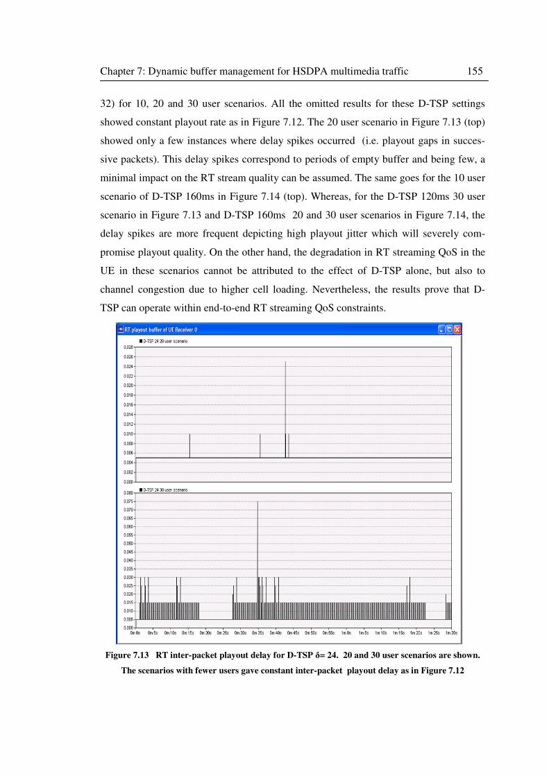
Chapter 7: Dynamic buffer management for HSDPA multimedia traffic 155
32) for 10, 20 and 30 user scenarios. All the omitted results for these D-TSP settings
showed constant playout rate as in Figure 7.12. The 20 user scenario in Figure 7.13 (top)
showed only a few instances where delay spikes occurred (i.e. playout gaps in succes-
sive packets). This delay spikes correspond to periods of empty buffer and being few, a
minimal impact on the RT stream quality can be assumed. The same goes for the 10 user
scenario of D-TSP 160ms in Figure 7.14 (top). Whereas, for the D-TSP 120ms 30 user
scenario in Figure 7.13 and D-TSP 160ms 20 and 30 user scenarios in Figure 7.14, the
delay spikes are more frequent depicting high playout jitter which will severely com-
promise playout quality. On the other hand, the degradation in RT streaming QoS in the
UE in these scenarios cannot be attributed to the effect of D-TSP alone, but also to
channel congestion due to higher cell loading. Nevertheless, the results prove that D-
TSP can operate within end-to-end RT streaming QoS constraints.
Figure 7.13 RT inter-packet playout delay for D-TSP δ= 24. 20 and 30 user scenarios are shown.
The scenarios with fewer users gave constant inter-packet playout delay as in Figure 7.12
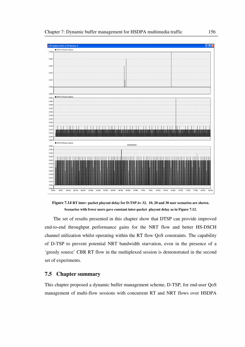
Chapter 7: Dynamic buffer management for HSDPA multimedia traffic 156
Figure 7.14 RT inter- packet playout delay for D-TSP δ= 32. 10, 20 and 30 user scenarios are shown.
Scenarios with fewer users gave constant inter-packet playout delay as in Figure 7.12.
The set of results presented in this chapter show that DTSP can provide improved
end-to-end throughput performance gains for the NRT flow and better HS-DSCH
channel utilization whilst operating within the RT flow QoS constraints. The capability
of D-TSP to prevent potential NRT bandwidth starvation, even in the presence of a
‘greedy source’ CBR RT flow in the multiplexed session is demonstrated in the second
set of experiments.
7.5 Chapter summary
This chapter proposed a dynamic buffer management scheme, D-TSP, for end-user QoS
management of multi-flow sessions with concurrent RT and NRT flows over HSDPA
Chapter 7: Dynamic buffer management for HSDPA multimedia traffic 157
downlink. D-TSP incorporates dynamic time priority switching to E-TSP, a time-space
priority queue management with Iub flow control mechanisms. The priority switching is
controlled via a parameter δ related to the RT flow delay budget, while a discard timer
drops RT packets likely to violate the end-to-end maximum QoS delay constraint.
Comparative performance study between D-TSP and E-TSP were undertaken via
extensive system-level HSDPA simulations. End-to-end TCP-based NRT throughput
was observed in a test multimedia receiver, including cases where multiple users share
the HSDPA channel. The experiments reveal that throughput gain is achieved (with
higher HSDPA channel load) with D-TSP compared to E-TSP, and, depending on the
setting of δ, VoIP packet discard can be kept within QoS bounds. D-TSP not only
increases UTRAN resource utilization by averting potential stalling of the NRT flow, but
also improves HSDPA channel utilization. Finally, D-TSP provides real-time QoS
optimization of the various flow components of the multimedia session of the same UE
at the air interface. Hence, D-TSP can complement the semi-real-time buffer optimiza-
tion strategy proposed in chapter 4, with the latter providing coarse QoS optimization
fine-tuned by the former.
158
Chapter 8
Conclusions and Future Work
8.1 Summary of the thesis
The aim of the Ph.D. project presented in this thesis, was to propose and analyze a set of
solutions to address the problem of quality of service provisioning and management of
multimedia sessions composed of diverse multiple flows with different quality of service
requirements in incumbent mobile wireless networks. The solutions proposed were
based on a novel queuing system that provides customized preferential treatment to the
classes of flows according to their different quality of service requirements. The novel
queuing system provided a base for development of buffer management schemes for
quality of service control and optimization at the air interface bottleneck of the state-of-
the-art High-Speed Downlink Packet Access System (HSDPA), a 3.5G mobile system
standardized by 3GPP as an enhancement to the widely deployed 3G Universal Mobile
Telecommunications Systems (UMTS). The main findings and contributions of the
research project can be summarized as follows.
8.1.1 Definition of a novel Time-Space Priority queuing system (TSP)
In most multi-flow queuing situations, the diverse flows possess different characteristics
and can usually be classed into real-time class for delay sensitive traffic with partial loss
tolerance, and non-real-time class for traffic that is loss sensitive and delay tolerant. In
order to jointly optimize both requirements, a priority queuing mechanism that can
provide delay prioritization for the real-time class, whilst allowing the non-real-time
class to have loss prioritization is essential. In the literature survey (chapter 2), it was
Chapter 8: Conclusions 159
found that most existing priority queuing solutions were based on single priority; i.e.
either loss prioritization, in which the queue capacity is dimensioned to allow a higher
loss priority class to gain preferential access in order to minimize the loss rate at the
expense of the other class(es), or delay prioritization, where the service discipline in the
queue allows preferential transmission of one class to minimize its delay/jitter of the
priority class at the expense of that of other class(es). Investigation of these priority
queuing disciplines in previous research were driven by the needs of the systems at the
time; for example in ATM, most priority queuing focused on loss prioritization schemes
such as partial buffer sharing (PBS) or pushout schemes because the low transmission
delay (relative to queuing delay) eliminated the need for delay prioritization in the
queuing.
The proposed Time-Space Priority (TSP) queuing incorporates delay prioritization
by attaching time (service) priority to the real-time class; but it also restricts real-time
class admission into the queue in order to provide loss prioritization to the non-real-time
class which is allowed unlimited access to the queue (i.e. space priority). The real-time
class packets are queued ahead of the non-real-time packets, but the threshold restricting
their admission enables the loss tolerance of the real-time flow to be exploited to further
minimize non-real-time loss and acts also to some extent as a (non-real-time class)
starvation mitigation mechanism. Furthermore, the TSP queuing minimizes jitter in the
real-time class. In a saturated (full) queue, a displacement policy can allow real-time
packets to drop non-real-time packets (up to the real-time class admission threshold
limit) from the TSP queue in order to curb excessive real-time packet losses.
In chapter 4, TSP is presented and analyzed by stochastic-analytic models along
with validation of the models using discrete event simulation. The analyses provided
insight into TSP behaviour under a range of multi-class traffic and queue configurations
indicating that through careful selection of the queue configuration (real-time flow
admission threshold), TSP queuing can provide optimized joint QoS control of the
loss/delay requirements of both classes of flows. Further comparative analyses with the
conventional priority queuing schemes showed that TSP queuing combined the advan-
tages of high buffer utilization, effectiveness in achieving optimum trade-off between
Chapter 8: Conclusions 160
the real-time and non-real-time flow QoS requirement, as well as simplicity of imple-
mentation.
8.1.2 Definition of adaptive QoS control strategy based on buffer threshold
optimization engine
The analyses of TSP in chapter 4 allowed a cost function to be derived in such a way
that a combined quality of service optimization is achievable to enable QoS control of
the classes in a multimedia session. The Weighted Grade of Service (WGoS) cost
function derived, takes into account traffic intensities of the real-time and non-real-time
class as well as the performance metrics that characterize the QoS of both traffic classes.
In the cost function, each of the considered performance metrics are weighted according
to their relative importance allowing for service class differentiation. Results of experi-
ments provided in chapter 4, showed that for different real-time and non-real-time traffic
mixes, the WGoS cost function enabled us to determine the optimum buffer threshold
i.e. the value of the TSP threshold that minimizes the WGoS for the given traffic confi-
guration.
Based upon the analyses, a strategy for adaptive configuration of the buffer thre-
shold by utilizing the TSP model as analytic engine for optimizing the threshold via the
WGoS cost function is proposed. This is motivated by the fact that analytical models are
well suited as kernels in optimization systems because they allow for fast processing;
and also because in a system like HSDPA where the strategy is applicable, changes in
traffic arrival rates and highly variable service (transmission) rates will necessitate
adaptive configuration of the TSP buffer threshold. The scheme involves measuring the
input traffic rates and service rates at the air interface which are then fed into an analytic
engine which utilizes the analytic model of the TSP buffer to determine the optimum
threshold that minimizes the cost function. Thus, at periodic intervals, or triggered by
other criteria, the parameters can be sampled again and a new optimum buffer value is
calculated. This allows for a coarse or semi-real-time adaptation of the buffer configura-
tion to changing QoS requirements to provide adaptive QoS control.
Chapter 8: Conclusions 161
8.1.3 Definition of flow control algorithm for HSDPA multimedia traffic
From the literature survey presented in chapter 2, it is clear that there is a growing trend
towards utilizing buffer management in mobile wireless networks as a means to facilitate
effective sharing of bottleneck air interface resources for enhanced end-to-end QoS
support. However, existing proposals have not addressed QoS support of multimedia
sessions with concurrent real-time and non-real-time classes/flows; whereas one of the
specified objectives of 3G systems and beyond is the requirement to support not only
traditional voice only or data only services but also multimedia services comprising
multiplexed flows in a single user session.
This thesis proposed a buffer management scheme based on TSP queuing system in
chapter 6 (Enhanced Time-Space priority, E-TSP buffer management), for HSDPA
multimedia sessions with real-time and non-real-time flows. The E-TSP buffer manage-
ment scheme incorporates additional flow control mechanism that employs a novel
credit-based flow control algorithm. The credit-based flow control algorithm is designed
to optimize the queuing at the air interface buffer (Node B) in response to time-varying
radio link quality of the mobile station receiving the multimedia traffic, as well as the
shared downlink channel load variation. Chapter 6 presented a performance evaluation
of E-TSP which showed that the flow control algorithm meets its objectives of efficient
utilization of buffer and radio link transmission resources resulting in improved higher
layer protocol performance and consequent end-to-end QoS enhancement. Thus, it can
be concluded from the investigation in chapter 6 that effective per session buffer man-
agement at the air interface of shared channels in a mobile system, can significantly
improve end-to-end traffic performance during multimedia sessions.
8.1.4 Definition of dynamic QoS optimization scheme for HSDPA multimedia
traffic
In chapter 7, a dynamic buffer management scheme (D-TSP) for HSDPA multimedia
session is proposed. D-TSP is based on the idea that the allocation of transmission
resources at the air interface can be optimized in real-time by dynamically switching the
time (transmission) priority between the real-time and non-real-time flows in the Time-
Chapter 8: Conclusions 162
Space Priority buffer. Given a transmission opportunity allocated to the mobile station
with multiplexed real-time and non-real-time flows, D-TSP can ensure that the real-time
flow gets just as much bandwidth as it requires to guarantee its QoS requirements, while
any unused spare capacity is automatically accorded to the non-real-time flow. That
way, the transmission resources allocated to the mobile station is optimized between the
two flows whilst also alleviating potential starvation of the non-real-time flow. D-TSP
relies on the estimation of the real-time flow delay budget in the base station buffer,
which is then used to control the transmission priority switching. Note that due to
statistical multiplexing in the HSDPA shared channel and stochastic nature of the service
process, the high variability necessitates a real-time optimization of the QoS control
between the real-time and non-real-time flows. As such, the adaptive buffer configura-
tion provided by the semi-real-time WGoS optimization engine can enable a coarse QoS
control which will be fine-tuned by the real-time dynamic scheme, D-TSP. Furthermore,
the dynamic priority switching of D-TSP will optimize the performance of the inter-user
packet scheduling algorithm employed in allocating the transmission time to the existing
mobile stations in the HSDPA cell.
In chapter 7, D-TSP is evaluated via extensive HSDPA simulations and the results
demonstrate the effectiveness of the system even when a greedy source constant bit-rate
real-time streaming flow is multiplexed with non-real-time data in an end-user multime-
dia session.
8.2 Suggestions for further research
Despite meeting the research objectives of proposing and evaluating solutions for
multimedia traffic QoS control and optimization in mobile networks, there still remain
areas of possible further investigations. One thing that is immediately apparent is that the
ideas presented in this thesis are not limited to HSDPA systems only but could find
applicability in other similar systems as well (especially at bottleneck points in a com-
munication system). The work in this thesis could be extended in several directions
including:
• Investigating the performance of the proposed WGoS optimization strategy on a
prototype and/or simulated mobile system. This aspect was outside the scope of
Chapter 8: Conclusions 163
the current research; but it would be desirable to assess the performance-
complexity trade-off for such a system with analytic optimization engine.
• Explore the utilization of WGoS based functions in other threshold-based priority
queuing systems such as partial buffer sharing.
• Development of analytical models for investigating Time-Space priority queuing
with flow control thresholds (E-TSP), and explore possible incorporation of the
analytical models in a WGoS based optimization system.
• Development of analytical models for investigating TSP with dynamic priority
switching, particularly as this concept will be useful for optimizing QoS control
in other types of priority queuing systems as well.
• Investigating the impact of Node B (air interface) buffer management on
(HSDPA) system capacity i.e. impact on performance of admission control algo-
rithms.
• Extending TSP to provide explicit priority control to enable layered prioritization
of real-time traffic such as video frames when multiplexed with non-real-time da-
ta in a multimedia session.
• Investigating the impact of TSP-based buffer management schemes on quality of
experience (QoE) to explore means for cross-layer optimization.
• Explore the adaptation of D-TSP time priority switching control parameter to en-
able D-TSP to cope with changing user channel quality and load
conditions/congestion on the HSDPA shared channel.
References 164
References [1] J. P. Castro, All IP in 3G CDMA Networks. Chichester, UK: John Wiley & Sons
Ltd., 2004.
[2] United Nations, "The Millennium Development Goals Report 2008," UN DESA,
2008 [Online]. http://mdgs.un.org/unsd/mdg/Resources/Static/Products/
Progress2008/MDG_Report_2008_En.pdf, [Accessed 6th Dec. 2008].
[3] J. F. DeRose, The Wireless Data Handbook, Fourth Edition. New York: John
Wiley & Sons, 1999.
[4] K. Pahlavan and A. Levesque, Wireless Information Networks. New York: John
Wiley & Sons, 1995.
[5] G. Peersman, S. Cvetkovic, P. Griffiths, and H. Spear, "The Global System for
Mobile Communications Short Messaging Service," IEEE Personal Communica-
tions, vol. 7(3), pp. 15-23, Jun. 2000.
[6] B. Walke, P. Seidenberg, and M. P. Althoff, UMTS, The Fundamentals. Chiche-
ster: John Wiley & Sons, 2003.
[7] GSM Association "GSM association home page" [Online] Available:
http://www.gsmworld.com/index [Accessed, 4 December 2008].
[8] G. Heine, GSM Networks: Protocols, Terminology, and Implementation. Nor-
wood, MA: Artech House, 1999.
[9] European Telecommunications Standards Institute, "Digital Cellular Telecom-
munications System (Phase 2+); High Speed Circuit Switched Data (HSCSD) –
Stage 2 (GSM 03.34)," ETSI TS 101 038 Version 5.0.1, Apr.1997.
[10] M. Hakaste, E. Nikula, and S. Hamiti, "GSM/EDGE Standards Evolution (up to
Rel’4)," in GSM, GPRS and EDGE Performance, T. Halonen, J. Romero, and J.
Melero, Eds., Second ed. Chichester, UK: John Wiley & Sons, Ltd, 2003.
[11] European Telecommunications Standards Institute, " Digital Cellular Telecom-
munications System (Phase 2+); General Packet Radio Service (GPRS); Overall
Description of the GPRS Radio Interface – Stage 2 (GSM 03.64)." ETSI TS 03
64 Version 5.1.0, Nov. 1997.
[12] R. J. Bates, GPRS – General Packet Radio Service. New York: McGraw-Hill,
2002.
[13] J. Cai and D. J. Goodman, "General Packet Radio Service in GSM," IEEE
Communications Magazine, pp. 122-131, Oct. 1997.
[14] G. Brasche and B. Walke, "Concepts, Services, and Protocols of the New GSM
Phase 2+ General Packet Radio Service," IEEE Communications Magazine vol.
35(8), pp. 94-104, Aug. 1997.
[15] A. Furuskar, S. Mazur, F. Muller, and H. Olofsson, "EDGE: enhanced data rates
for GSM and TDMA/136 evolution," IEEE Personal Communications, vol. 6,
pp. 56-66, Jun. 1999.
References 165
[16] T. Halonen, J. Romero, and J. Melero, GSM, GPRS and EDGE Performance
Chichester, UK: John Wiley & Sons, Ltd, 2003.
[17] E. Seurre, P. Savelli, and P.-J. Pietri, EDGE for Mobile Internet. Norwood, MA:
Artech House, 2003.
[18] R. E. Sherrif and Y. F. Hu, Mobile Satellite Communication Networks. Chiche-
ster, UK: John Wiley & Sons, Ltd., 2001.
[19] European Telecommunications Standards Institute, "Universal Mobile Telecom-
munications Systems (UMTS), Requirements for the UMTS Terrestrial Radio
Access Systems (UTRA)," ETSI Technical Report, UMTS 21.01 version 3.0.1
Nov. 1997.
[20] H. Holma and A. Toskala, WCDMA for UMTS-HSPA Evolution and LTE: John
Wiley & Sons Ltd, 2007.
[21] A. Golaup, O. Holland, and A. H. Aghvami, "Concept and Optimization of an
effective Packet Scheduling Algorithm for Multimedia Traffic over HSDPA," in
Proc. IEEE International Symposium on Personal, Indoor and Mobile Radio
Communications. Berlin, Germany, 2005.
[22] 3GPP, "High Speed Downlink Packet Access; Overall Description," 3GPP TR
25.308 version 5.7.0, Dec. 2004.
[23] 3GPP, "Medium Access Control (MAC) protocol specification," 3GPP TS
25.321 version 7.5.0, Jun. 2007.
[24] L. Chuang and L. Yin., "Dynamic partial buffer sharing scheme: Proportional
packet loss rate," in Proc. ICCT2003, 2003, pp. 259-262.
[25] J. W. Causey and H. S. Kim, "Comparison of buffer allocation schemes in ATM
switches: Complete sharing, partial sharing, and dedicated allocation," in Proc.
International Conference on Communications, vol. 2, May 1994, pp. 1164-1168.
[26] M. G. Hluchyj and M. J. Karol, "Queueing in high performance packet switch-
ing," IEEE J. Selected Areas in Commun., vol. SAC-6. no. 9, Dec. 1988.
[27] T. Czachovski and F. Peregrine, "A Queuing Model for Optimal Control of
Partial Buffer Sharing," ATM Computer Operation Research, vol. 25(2), pp. 113-
126., Feb. 1998.
[28] C. G. Kang and H. H. Tan, "Queuing analysis of explicit priority assignment
partial buffers sharing schemes for ATM networks" in Proc. IEEE/ACM
INFOCOM, Mar. 1993, pp. 810-819.
[29] H. Kroner, "Comparative Performance Study of Space Priority Mechanisms for
ATM Networks " in Proc. IEEE INFOCOM ’90, June 1990, pp. 1136-1143.
[30] G. Gallassi, G. Rigolio, and L. Fratta, " Bandwidth Assignment in Prioritized
ATM Networks," in Proc. IEEE GLOBECOM ’90, Dec. 1990 pp. 852-856.
[31] K. Bala, I. Cidon, and K. Sohraby, "Congestion Control for High Speed Packet
Switched Network," in Proc. IEEE INFOCOM ’90, Jun. 1990, pp. 520-526.
References 166
[32] G. Hetbuterne and A. Gravey, "A Space Priority Queueing Mechanism for
Multiplexing ATM Channels," Computer Networks and systems, pp. 37-43,
1990.
[33] J. J. Bae, T. Suda, and R. Simha, "Analysis of a Finite Buffer Queue with Hete-
rogeneous Markov Modulated Poisson Arrival Processes: A Study of Traffic
Burstiness and Priority Packet Discarding," in Proc. IEEE INFOCOM ’92, Aug.
1992.
[34] H. Kroner, G. Herbuterne, P. Boye, and A. Gravey, "Priority Management in
ATM Switching Nodes," IEEE Journal on Selected Areas in Communications,
vol. 9, pp. 418-427, Apr. 1991
[35] J.-w. Cho and D.-h. Cho, "Dynamic buffer management scheme based on rate
estimation in packet-switched networks," Computer Networks, vol. 39, Issue 6,
pp. 769-787, 21 Aug. 2002.
[36] D. Mitra and I. Ziedins, "Virtual partitioning by dynamic priorities: Fair and
efficient resource-sharing by several services," in Broadband Communications:
Network Services, Applications, Future Directions, Lecture Notes in Computer
Science: Spinger Verlag, 1996, pp. 173-185.
[37] L. Georgiadis, I. Cidon, R. Guerin, and A. Khamisy, "Optimal Buffer Sharing,"
IEEE J. Select. Areas Commun., vol. 13, pp. 1229-1240, Sep. 1995.
[38] H. Yousefi'zadeh and E. A. Jonckheere, "Dynamic neural-based buffer manage-
ment for queuing systems with self-similar characteristics," IEEE Transactions
on Neural Networks vol. 16, no.5, pp. 1163-1173, Sept. 2005.
[39] G.-L. Wu and J. W. Mark, "A Buffer Allocation Scheme for ATM Networks:
Complete Sharing Based on Virtual Partition," IEEE/ACM Transactions on Net-
working, vol. 3, no. 6, Dec. 1995.
[40] A. Y. M. Lin and J. Silvester, "Priority Queuing Strategies and Buffer Allocation
Protocols for Traffic Control at an ATM Integrated Broadband Switching Sys-
tem" IEEE Journal on Selected Areas in Communications, vol. SAC-9, no. 9, pp.
1524- 1536, Dec. 199l.
[41] J. M. Pitts and J. A. Schormans, Introduction to IP and ATM Design and Perfor-
mance, Second ed. Chichester, UK: John Wiley & Sons, 2000.
[42] A. K. Choudhury and E. L. Hahne, "Space priority management in a shared
memory ATM switch " in Proc. IEEE GLOBECOM 93, vol. 3, 1993, pp. 1375-
1383.
[43] A. Demers, S. Keshavt, and S. Shenkar, "Analysis and Simulation of a Fair
Queuing algorithm," in Proc. ACM SIGCOMM’89, Austin, TX, Sep. 1989, pp. 1-
12.
[44] L. Zhang, "VirtualClock: a new traffic control algorithm for packet-switched
networks," ACM Transactions on Computer Systems vol. 9 (2), pp. 101-124, May
1991.
[45] A. Gulati, A. Merchant, and P. J. Varman, "pClock: an arrival curve based
approach for QoS guarantees in shared storage systems.," in Proc. 2007 ACM
References 167
SIGMETRICS international Conference on Measurement and Modeling of Com-
puter Systems (ACM SIGMETRICS '07). San Diego, California, USA, June 12 -
16, 2007, pp. 13-24.
[46] D. Stiliadis and A. Varma, "Efficient fair queueing algorithms for packet-
switched networks," IEEE/ACM Transactions on Networking, vol. 6 (2), pp. 175-
185, Apr. 1998.
[47] P. Goyal, H. M. Vin, and H. Cheng, "Start-time fair queueing: a scheduling
algorithm for integrated services packet switching networks," IEEE/ACM Trans-
actions on Networking vol. 5 (5), pp. 690-704, Oct. 1997.
[48] M. Irland, "Buffer Management in a Packet Switch," IEEE Transactions on
Communications, vol. 26, no. 3, pp. 328-337, Mar. 1978.
[49] F. Kamoun and L. Kleinrock, "Analysis of Shared Finite Storage in a Computer
Network Node Environment Under General Traffic Conditions," IEEE Transac-
tions on Communications vol. 28, no.7, pp. 992-1003, Jul. 1980.
[50] K. Rothermel, "Priority mechanisms in ATM networks," in Proc. IEEE
GLOBECOM '90, vol. 2, Dec. 1990, pp. 847-851
[51] S. Sumita and T. Ozawa, "Achievability of Performance Objectives in ATM
Switching Nodes," in Proc. International Seminar on Performance of Distributed
and Parallel Systems. Kyoto, Japan, Dec. 7-9, 1988, pp. 45-56.
[52] H. Kroner, "Buffer Access Mechanisms for Multiplexing of Different Traffic
Classes in an ATM Network," Race Document. UST-123-008-CD-CC, Apr. 25,
1989.
[53] T. C. Hou and A. K. Wong, "Queueing Analysis for ATM Switching of Mixed
Continuous-Bit-Rate and Bursty Traffic," in Proc. IEEE INFOCOM '90, Jun.
1990, pp. 660-667.
[54] H. J. Chao and N. Uzun, "An ATM queue manager with multiple delay and loss
priorities," in Proc. IEEE GLOBECOM '92, vol. 1, 6-9 Dec 1992, pp. 308-313
[55] S. Kausha and R. K. Sharma, "Modelling and analysis of adaptive buffer sharing
scheme for consecutive packet loss reduction in broadband networks," Interna-
tional Journal of Computer Systems Science and Engineering, vol. 4, no. 1,
Winter 2008.
[56] I. Awan and K. Al-Begain, "An Analytical Study of Quality of Service Provi-
sioning for Multi-service Mobile IP Networks Using Adaptive Buffer
Management," in Proc. 11th International Conference on Analytical and Sto-
chastic Modelling Techniques and Applications (ASMTA04). Magdeburg,
Germany, Jun. 2004, pp. 166-172.
[57] Z. Orlov and M. C. Necker, "Enhancement of Video Streaming QoS with Active
Buffer Management in Wireless Environments," in Proc. 13th European Wire-
less 2007 (EW 2007). Paris, 2007.
[58] S. Kozlov, P. v. d. Stok, and J. Lukkien, "Adaptive Scheduling of MPEG Video
Frames During Real-time Wireless Video Streaming," in Proc. 6th Int. Sympo-
sium on a World of Wireless Mobile and Multimedia Networks, 2005.
References 168
[59] Y. Bai and M. R. Ito, "Application-Aware Buffer Management: New Metrics and
Techniques," IEEE Transactions on Broadcasting, vol. 51 no. 1, pp. 114-121,
Mar. 2005.
[60] G. Liebl, H. Jenkac, T. Stockhammer, C. Buchner, and A. Klein, "Radio Link
Buffer Management and Scheduling for Video Streaming over Wireless Shared
Channels " in Proc. 14th International Packet Video Workshop (PVW 2004). Ir-
vine, CA, USA, Dec. 2004.
[61] I. Awan and K. Al-Begain, "Maintaining QoS Through Preferential Treatment to
UMTS Services," International Journal of Simulation, vol. 4 No. 5-6, pp. 59-65,
Dec. 2003.
[62] J. Tang, G. Feng, C.-K. Siew, and L. Zhang, "Providing Differentiated Services
Over Shared Wireless Downlink Through Buffer Management," IEEE Transac-
tions on Vehicular Technology, vol. 57, no.1, pp. 548-555, Jan. 2008.
[63] H.-C. Yang and S. Sasankan, "Analysis of Channel-Adaptive Packet Transmis-
sion Over Fading Channels With Transmit Buffer Management," IEEE
Transactions on Vehicular Technology, vol. 57, no.1, pp. 404-413, Jan. 2008.
[64] S. Jain and E. Modiano, "Buffer management schemes for enhanced TCP per-
formance over satellite links," in Proc. IEEE Military Communications
Conference, 2005. MILCOM 2005 vol. 3, 17-20 Oct. 2005, pp. 1672-1678.
[65] M. S. Obaidat, C. B. Ahmed, and N. Boudriga, "DRA: a new buffer management
scheme for wireless atm networks using aggregative large deviation principle,"
Computer Communications, vol. 26 (2003), pp. 708-717, 2003.
[66] E. Reguera and F. J. Velez, "Enhanced UMTS Services and Applications: A
Perspective Beyond 3G," in Proc. IEE 5th European Personal Mobile Communi-
cations Conference, Apr. 2003.
[67] 3GPP, "Quality of Service (QoS) concept and architecture," TS 23.107 version
8.0.0, Dec. 2008.
[68] D. Soldani, M. Li, and R. Cuny, QoS and QoE Management in UMTS Cellular
Systems: John Wiley and Sons Ltd., 2006.
[69] H. Holma and A. Toskala, WCDMA for UMTS: Radio Access for Third Genera-
tion Mobile Communications: Jonh Wiley & Sons Ltd., 2001.
[70] M. Ghanderi and R. Boutaba, "Call Admission Control in Mobile Cellular
Networks: A Comprehensive Survey," Wireless Communications and Mobile
Computing, vol. 6 (1), 2006.
[71] W. Ahmad and I. Awan, "Performance evaluation of CAC Schemes for Multi-
service Traffic Environment in 3G Networks," Simulation, vol. 83(3), Mar. 2007.
[72] K. I. Pedersen, "Quality Based HSDPA Access Algorithms," in Proc. IEEE
Vehicular Technology Conference (VTC Fall 2005), Sept. 2005.
[73] K. I. Pedersen, A. Toskala, and P. E. Mogensen, "Mobility Management and
Capacity Analysis for High Speed Downlink Packet Access in WCDMA," in
Proc. IEEE Vehicular Technology Conference (VTC Fall 2004), 2004.
References 169
[74] K. I. Pedersen, P. E. Mogensen, and T. E. Kolding, "Overview of QoS Options
for HSDPA," IEEE Communications Magazine, pp. 100-105, Jul. 2006.
[75] P. A. Gutierrez, "Packet Scheduling and Quality of Service in HSDPA," PhD
Thesis, Institute of Electronic Systems, Aalborg University, Denmark, Oct. 2003.
[76] R. C. Elliott and W. A. Krzymien, "Scheduling algorithms for the cdma2000
packet data evolution," in Proc. IEEE 56th Vehicular Technology Conference
(VTC 2002-Fall), vol. 1, 2002, pp. 304-310.
[77] M. Andrews et al., "Providing Quality of Service over a shared wireless link,"
IEEE Communications Magazine, Feb. 2001.
[78] A. K. F. Khattab and K. M. F. Elsayed, "Channel-quality dependent earliest due
fair scheduling schemes for wireless multimedia networks," in Proc. MSWiM
2004. Venice, Italy, Oct. 2004.
[79] G. Barriac and J. Holtzman, "Introducing Delay Sensitivity into the Proportional
Fair Algorithm for CDMA Downlink Scheduling," in Proc. IEEE International
Symposium on Spread Spectrum Techniques and Applications, September 2002,
pp. 652-656.
[80] O. Holland, A. Golaup, and H. Aghvami, "Efficient Packet Scheduling for
HSDPA Allowing Inter-class Prioritization," IET Electronics Letters, vol. 42. no.
18, Aug. 2006.
[81] 3GPP, "High Speed Downlink Packet Access; Overall Description," 3GPP TR
25.308 version 5.7.0, Dec. 2004.
[82] 3GPP, "Radio Link Control (RLC) protocol specification," TS 25.322 version
5.13.0, Dec. 2005.
[83] SEACORN, "End-to-End Network Model for Enhanced UMTS," Deliverable
D3.2v2, Oct. 2003.
[84] 3GPP, "Physical channels and mapping of transport channels onto physical
channels (FDD)," 3GPP TS 25.211 Version 5.0.0, Mar. 2002.
[85] H. Holma and A. Toskala, HSDPA/HSUPA for UMTS: John Wiley & Sons Ltd,
2006.
[86] 3GPP, "High Speed Downlink Packet Access : Iub/Iur protocol aspects," 3GPP
TS 25.877 Version 5.4.0, Release 5, Jun. 2002.
[87] Y. Takagi, S. Hino, and T. Takabashi, "Priority assignment control of ATM line
buffers with multiple QOS Classes," IEEE J. Select. Areas in communications,
pp. 1078-1092, Sep. 1991.
[88] G. M. Woodruff and R. Kositpaiboon, "Multimedia traffic management prin-
ciples for guaranteed ATM network performance," IEEE J. Selected Areas in
communications. , vol. 8, pp. 437-446, Apr. 1990.
[89] A. A. Lazer, A. Temple, and R. Gidron, "An architecture for integrated networks
that guarantees quality of service," International Digital Analog Communications
systems journal, vol. 3, no. 2, pp. 229–238, Apr.–Jun. 1990.
References 170
[90] B. Beutel, "Integration of the Petri Net tool TimeNet into the MOSEL environ-
ment," Masters Thesis DA-14-2002-17, Department of Computer Science,
University of Erlangen, Germany, 2003.
[91] K. Al-Begain, G. Bolch, and H. Herold, Practical performance modeling-
Application of the MOSEL language: Kluwer Academic publishers, 2001.
[92] G. Ciardo, R. M. Fricks, J. Muppala, and K. S. Trivedi, "SPNP Users Manual
Version 4.0," Duke University, Department of Electrical Engineering, Durham,
NC. Mar. 1994.
[93] G. Bolch, S. Greiner, H. Jung, and R. Zimmer, "The Markov Analyzer MOSES,"
Technical Report TR-i4-10-94, IMMD IV, Univ. of Erlangen-Nuremberg, 1994.
[94] R. German, C. Kelling, A. Zimmermann, and G. Hommel, "TimeNeT- a toolkit
for evaluating non-markovian stochastic petri nets," Technical report, Technical
University of Berlin, Berlin, 1994.
[95] K. Al-Begain, J. Barner, G. Bolch, and A. I. Zriekat online, "The performance
and Reliability Modelling Language MOSEL and its Application," International
Journal of Simulation: Systems, Science and Technology vol. 3, no. 3-4, pp. 66-
80, 2002.
[96] A. I. Zriekat, S. Y. Yerima, and K. Al-Begain, " Performance Evaluation and
Resource Management of Hierarchical MACRO-/MICRO Cellular Networks Us-
ing MOSEL-2," Wireless Personal Communications, vol. 44 , Issue 2 pp. 153 -
179, Jan. 2008.
[97] P. Wüchner, K. Al-Begain, J. Barner, and G. Bolch, "Modelling a single
GSM/GPRS cell with delay tolerant voice calls using MOSEL-2," in Proc. UK
Simulation Conference (UKSIM '04). Oxford, UK, May 2004, pp. 88-94.
[98] J. Roszik, C. S. Kim, and J. Sztrik, "Modelling Cellular Networks Using Mosel,"
Technical Report No. 2003/14, Institute of Informatics, University of Debrecen,
Hungary 2003.
[99] Y. Li, K. Al-Begain, and I. Awan, "Performance modelling of GSM/GPRS
mobile system with MOSEL," in Proc. 4th PGNet. Liverpool, Jun. 2003, pp.
245-250.
[100] G. Bolch, S. Greiner, H. D. Meer, and K. S. Trivedi, Queueing Networks and
Markov Chains: John Wiley & Sons Ltd., 1998.
[101] P. Wüchner, H. D. Meer, J. Barner, and G. Bolch, "A brief Introduction to
MOSEL-2," in Proceedings of 13th GI/ITG Conference: Measuring Modeling
and Evaluation of Computer and Communication Systems. Nürnberg, Germany,
2006, pp. 473-476.
[102] S. Dixit, Y. Guo, and Z. Antoniou, "Resource Management and Quality of
Service in Third-Generation Wireless Networks," IEEE Commun. Mag, vol. 39,
pp. 125–133, Feb. 2001.
[103] W. Bang, K. I. Pedersen, T. E. Kolding, and P. E. Mogensen, "Performance of
VoIP on HSDPA," in Proc. IEEE VTC. Stockholm, Jun. 2005.
References 171
[104] ITU, "Guidelines for Evaluation of Radio Transmission Technologies for IMT-
2000," Recommendation ITU-R M.1225, 1997.
[105] 3GPP, "Physical Layer Aspects of UTRA High Speed Downlink Packet Access
(Release 4)," TR 25.848 version 5.13.0, Mar. 2001.
[106] W. S. Jeong, D. G. Jeong, and B. Kim, "Packet Scheduler for Mobile Internet
Services Using High Speed Downlink Packet Access," IEEE Transactions on
Wireless Communications, vol. 3, no.5, Sep. 2004.
[107] H. van den Berg, R. Litjens, and J. Laverman, "HSDPA flow level performance:
the impact of key system and traffic aspects," in Proc. 7th ACM international
symposium on Modeling, analysis and simulation of wireless and mobile systems,
2004, pp. 283 - 292.
[108] M. C. Necker and A. Weber, "Impact of Iub flow control on HSDPA System
Performance," in Proc. Personal Indoor and Mobile Radio Communications
(PIMRC 2005). Berlin, Germany, Sep. 2005.
[109] P. J. Legg, "Optimised Iub flow control for UMTS HSDPA," in Proc. IEEE
Vehicular Technology Conference (VTC 2005 Spring). Stockholm, Sweden, Jun.
2005.
[110] T. L. Weerawardane, A. Timm-Giel, C. Gorg, and T. Reim, "Impact of the
Transport Network Layer Flow Control for HSDPA performance," in Proc. IEE
2006 Conference. Colombo Sri Lanka, Sep. 2006.
[111] T. Weerawardane, "Preventive and Reactive based TNL Congestion Control
Impact on the HSDPA performance," in Proc. IEEE Vehicular Technology Con-
ference. May 2008, Singapore.
[112] 3GPP, "UTRAN Iur interface user plane protocols for Common Transport
Channel data streams," 3GPP TS 25.425 Version 5.2.0, Release 5, Sep. 2002.
[113] H. Balakrishnan, V. N. Padmanabhan, S. Seshan, and Y. H. Katz, "A Compari-
son of Mechanisms for Improving TCP Performance over Wireless Links," in
Proc. ACM SIGCOMM, Aug. 1996.
[114] G. Xylomenos, G. C. Polyzos, P. Mahonen, and M. Saaranen, "TCP Performance
Issues over Wireless Links," IEEE Communications Magazine, Apr. 2001.
[115] A. Alexiou, C. Bouras, and V. Igglesis, "Performance Evaluation of TCP over
UMTS Transport Channels," in Proc. 7th International Symposium on Commu-
nications Interworking, INTERWORKING 2004. Ottawa, Canada, Dec. 2004.
[116] M. Assaad and D. Zeghlache, "Cross-Layer Design in HSDPA System to Reduce
the TCP Effect," IEEE Journal on Selected Areas in Communications, vol. 24,
no. 3, Mar. 2006.
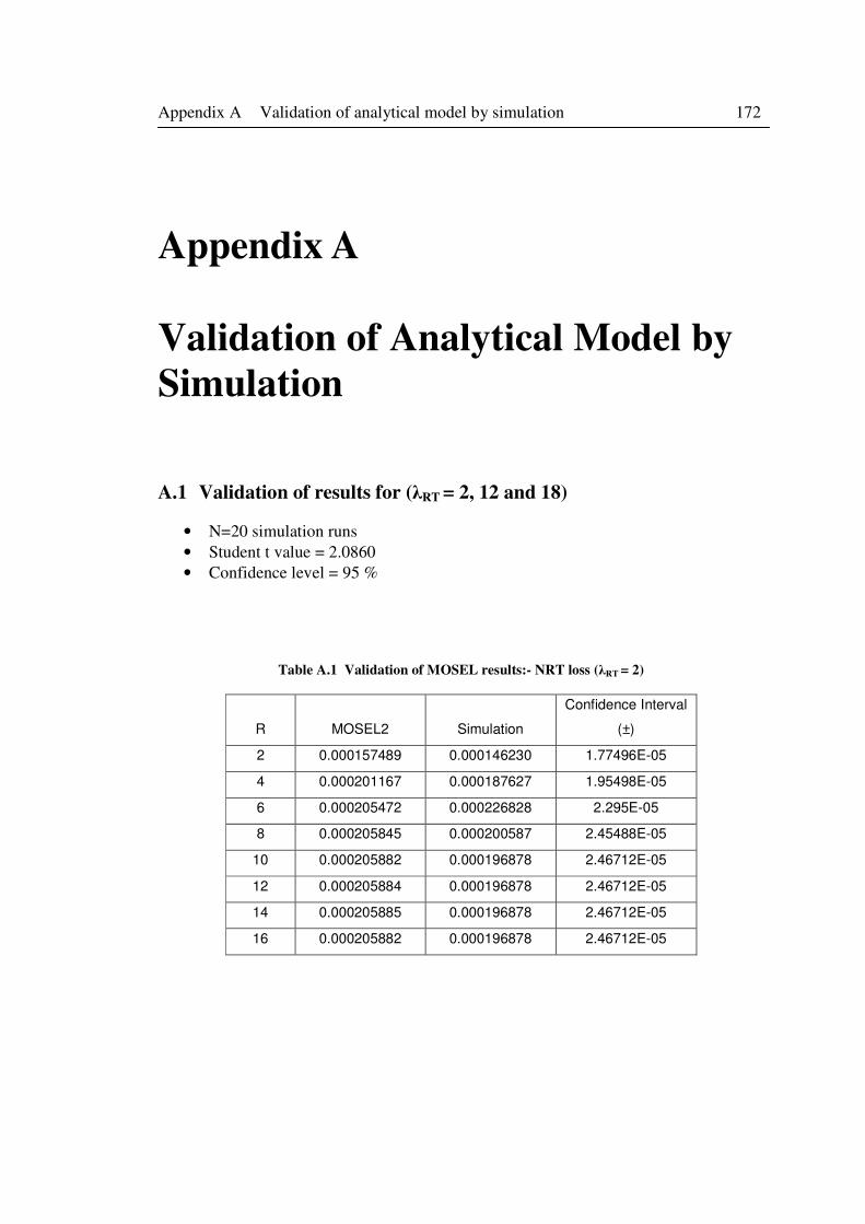
Appendix A Validation of analytical model by simulation 172
Appendix A
Validation of Analytical Model by
Simulation
A.1 Validation of results for (λRT = 2, 12 and 18)
• N=20 simulation runs
• Student t value = 2.0860
• Confidence level = 95 %
Table A.1 Validation of MOSEL results:- NRT loss (λRT = 2)
R MOSEL2 Simulation
Confidence Interval
(±)
2 0.000157489 0.000146230 1.77496E-05
4 0.000201167 0.000187627 1.95498E-05
6 0.000205472 0.000226828 2.295E-05
8 0.000205845 0.000200587 2.45488E-05
10 0.000205882 0.000196878 2.46712E-05
12 0.000205884 0.000196878 2.46712E-05
14 0.000205885 0.000196878 2.46712E-05
16 0.000205882 0.000196878 2.46712E-05
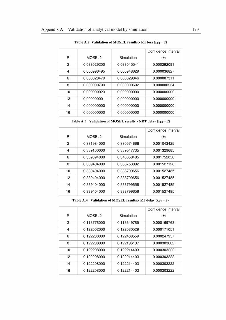
Appendix A Validation of analytical model by simulation 173
Table A.2 Validation of MOSEL results:- RT loss (λRT = 2)
R MOSEL2 Simulation
Confidence Interval
(±)
2 0.033029200 0.033045541 0.000292091
4 0.000996495 0.000948629 0.000036827
6 0.000028479 0.000029846 0.000007311
8 0.000000799 0.000000692 0.000000234
10 0.000000023 0.000000000 0.000000000
12 0.000000001 0.000000000 0.000000000
14 0.000000000 0.000000000 0.000000000
16 0.000000000 0.000000000 0.000000000
Table A.3 Validation of MOSEL results:- NRT delay (λRT = 2)
R MOSEL2 Simulation
Confidence Interval
(±)
2 0.331984000 0.330574666 0.001043425
4 0.339100000 0.339547735 0.001329685
6 0.339394000 0.340058485 0.001752056
8 0.339404000 0.338753092 0.001527128
10 0.339404000 0.338799656 0.001527485
12 0.339404000 0.338799656 0.001527485
14 0.339404000 0.338799656 0.001527485
16 0.339404000 0.338799656 0.001527485
Table A.4 Validation of MOSEL results:- RT delay (λRT = 2)
R MOSEL2 Simulation
Confidence Interval
(±)
2 0.118778000 0.118649785 0.000169763
4 0.122002000 0.122080529 0.000171051
6 0.122200000 0.122468559 0.000247957
8 0.122208000 0.122196137 0.000303602
10 0.122208000 0.122214403 0.000303222
12 0.122208000 0.122214403 0.000303222
14 0.122208000 0.122214403 0.000303222
16 0.122208000 0.122214403 0.000303222
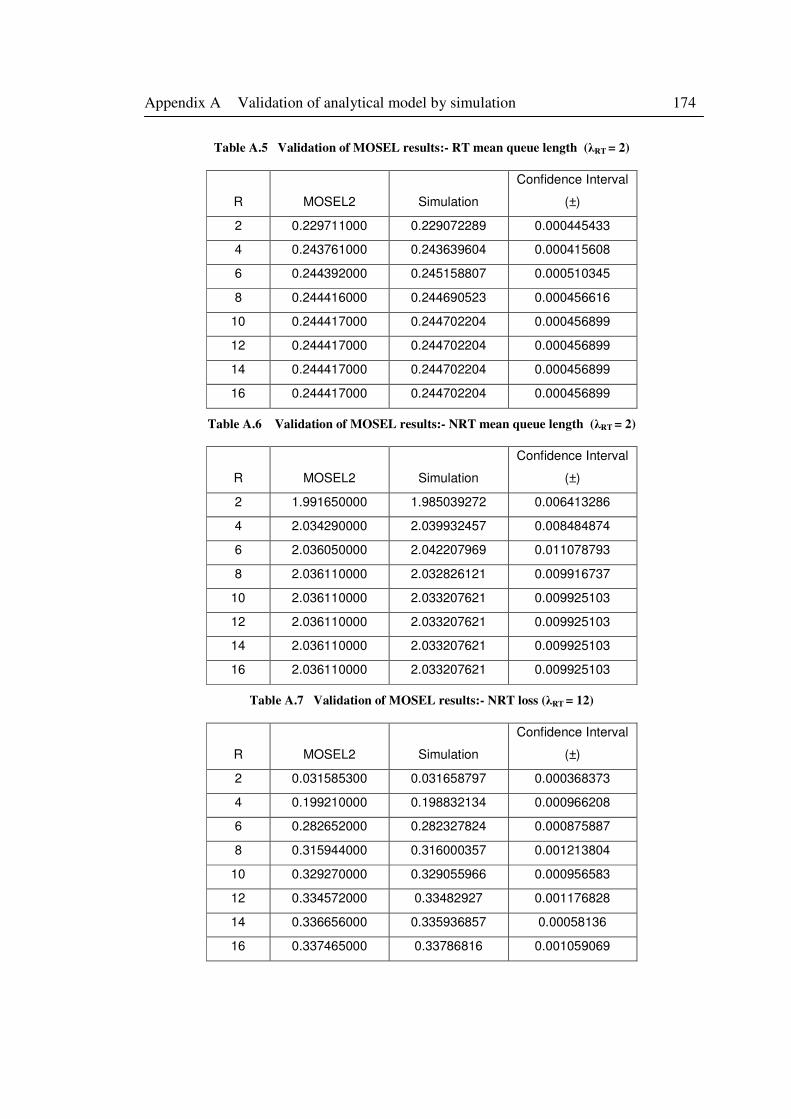
Appendix A Validation of analytical model by simulation 174
Table A.5 Validation of MOSEL results:- RT mean queue length (λRT = 2)
R MOSEL2 Simulation
Confidence Interval
(±)
2 0.229711000 0.229072289 0.000445433
4 0.243761000 0.243639604 0.000415608
6 0.244392000 0.245158807 0.000510345
8 0.244416000 0.244690523 0.000456616
10 0.244417000 0.244702204 0.000456899
12 0.244417000 0.244702204 0.000456899
14 0.244417000 0.244702204 0.000456899
16 0.244417000 0.244702204 0.000456899
Table A.6 Validation of MOSEL results:- NRT mean queue length (λRT = 2)
R MOSEL2 Simulation
Confidence Interval
(±)
2 1.991650000 1.985039272 0.006413286
4 2.034290000 2.039932457 0.008484874
6 2.036050000 2.042207969 0.011078793
8 2.036110000 2.032826121 0.009916737
10 2.036110000 2.033207621 0.009925103
12 2.036110000 2.033207621 0.009925103
14 2.036110000 2.033207621 0.009925103
16 2.036110000 2.033207621 0.009925103
Table A.7 Validation of MOSEL results:- NRT loss (λRT = 12)
R MOSEL2 Simulation
Confidence Interval
(±)
2 0.031585300 0.031658797 0.000368373
4 0.199210000 0.198832134 0.000966208
6 0.282652000 0.282327824 0.000875887
8 0.315944000 0.316000357 0.001213804
10 0.329270000 0.329055966 0.000956583
12 0.334572000 0.33482927 0.001176828
14 0.336656000 0.335936857 0.00058136
16 0.337465000 0.33786816 0.001059069
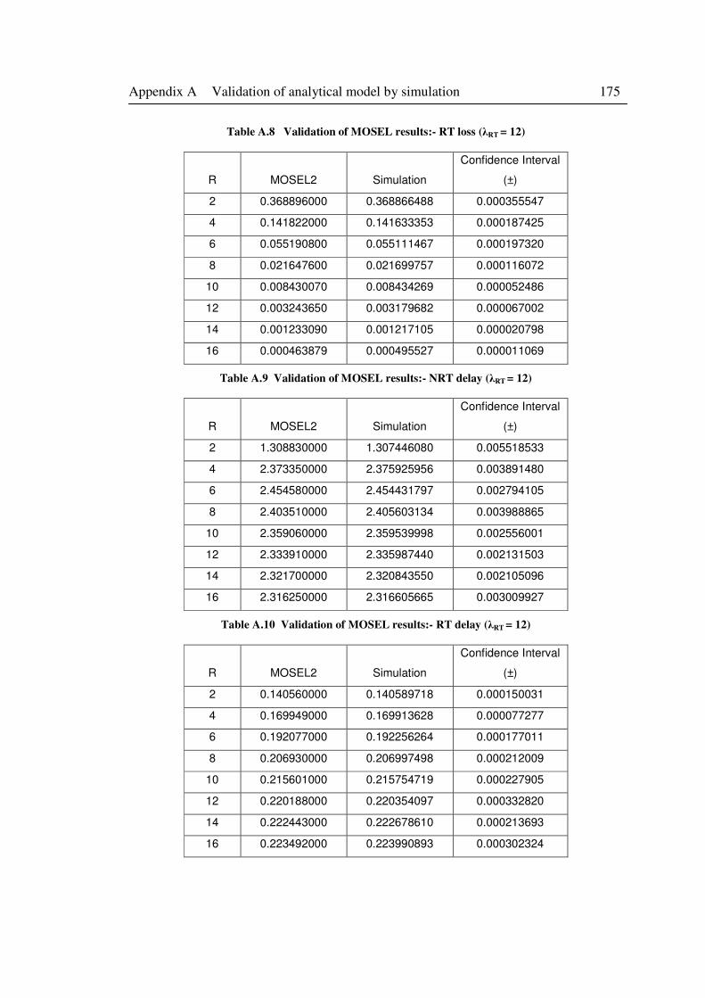
Appendix A Validation of analytical model by simulation 175
Table A.8 Validation of MOSEL results:- RT loss (λRT = 12)
R MOSEL2 Simulation
Confidence Interval
(±)
2 0.368896000 0.368866488 0.000355547
4 0.141822000 0.141633353 0.000187425
6 0.055190800 0.055111467 0.000197320
8 0.021647600 0.021699757 0.000116072
10 0.008430070 0.008434269 0.000052486
12 0.003243650 0.003179682 0.000067002
14 0.001233090 0.001217105 0.000020798
16 0.000463879 0.000495527 0.000011069
Table A.9 Validation of MOSEL results:- NRT delay (λRT = 12)
R MOSEL2 Simulation
Confidence Interval
(±)
2 1.308830000 1.307446080 0.005518533
4 2.373350000 2.375925956 0.003891480
6 2.454580000 2.454431797 0.002794105
8 2.403510000 2.405603134 0.003988865
10 2.359060000 2.359539998 0.002556001
12 2.333910000 2.335987440 0.002131503
14 2.321700000 2.320843550 0.002105096
16 2.316250000 2.316605665 0.003009927
Table A.10 Validation of MOSEL results:- RT delay (λRT = 12)
R MOSEL2 Simulation
Confidence Interval
(±)
2 0.140560000 0.140589718 0.000150031
4 0.169949000 0.169913628 0.000077277
6 0.192077000 0.192256264 0.000177011
8 0.206930000 0.206997498 0.000212009
10 0.215601000 0.215754719 0.000227905
12 0.220188000 0.220354097 0.000332820
14 0.222443000 0.222678610 0.000213693
16 0.223492000 0.223990893 0.000302324
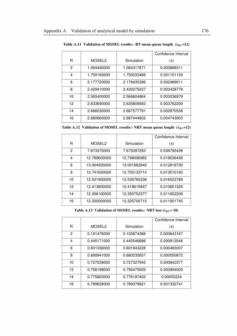
Appendix A Validation of analytical model by simulation 176
Table A.11 Validation of MOSEL results:- RT mean queue length (λRT =12)
R MOSEL2 Simulation
Confidence Interval
(±)
2 1.064490000 1.064317671 0.000888311
4 1.750160000 1.750033488 0.001151120
6 2.177720000 2.178435396 0.002489011
8 2.429410000 2.430275227 0.003428778
10 2.565400000 2.566604864 0.003036979
12 2.633690000 2.635809583 0.003762200
14 2.666030000 2.667577791 0.002870538
16 2.680660000 2.687444602 0.004743903
Table A.12 Validation of MOSEL results:- NRT mean queue length (λRT =12)
R MOSEL2 Simulation
Confidence Interval
(±)
2 7.673370000 7.670097250 0.036795436
4 12.789600000 12.798096982 0.018536436
6 13.004500000 13.001682840 0.012818730
8 12.741600000 12.750133714 0.013510193
10 12.531900000 12.530765336 0.016523785
12 12.413800000 12.418615847 0.010651325
14 12.356100000 12.350752377 0.011602208
16 12.330000000 12.325700715 0.011921745
Table A.13 Validation of MOSEL results:- NRT loss (λRT = 18)
R MOSEL2 Simulation
Confidence Interval
(±)
2 0.101476000 0.100874386 0.000643167
4 0.445171000 0.445546686 0.000813546
6 0.601336000 0.601943228 0.000483007
8 0.680941000 0.680235857 0.000550872
10 0.727039000 0.727327945 0.000842377
12 0.756198000 0.756475505 0.000994003
14 0.775820000 0.776197402 0.00055224
16 0.789628000 0.789379921 0.001332741
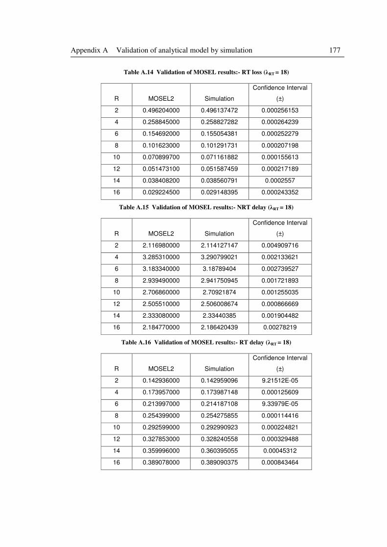
Appendix A Validation of analytical model by simulation 177
Table A.14 Validation of MOSEL results:- RT loss (λRT = 18)
R MOSEL2 Simulation
Confidence Interval
(±)
2 0.496204000 0.496137472 0.000256153
4 0.258845000 0.258827282 0.000264239
6 0.154692000 0.155054381 0.000252279
8 0.101623000 0.101291731 0.000207198
10 0.070899700 0.071161882 0.000155613
12 0.051473100 0.051587459 0.000217189
14 0.038408200 0.038560791 0.0002557
16 0.029224500 0.029148395 0.000243352
Table A.15 Validation of MOSEL results:- NRT delay (λRT = 18)
R MOSEL2 Simulation
Confidence Interval
(±)
2 2.116980000 2.114127147 0.004909716
4 3.285310000 3.290799021 0.002133621
6 3.183340000 3.18789404 0.002739527
8 2.939490000 2.941750945 0.001721893
10 2.706860000 2.70921874 0.001255035
12 2.505510000 2.506008674 0.000866669
14 2.333080000 2.33440385 0.001904482
16 2.184770000 2.186420439 0.00278219
Table A.16 Validation of MOSEL results:- RT delay (λRT = 18)
R MOSEL2 Simulation
Confidence Interval
(±)
2 0.142936000 0.142959096 9.21512E-05
4 0.173957000 0.173987148 0.000125609
6 0.213997000 0.214187108 9.33979E-05
8 0.254399000 0.254275855 0.000114416
10 0.292599000 0.292990923 0.000224821
12 0.327853000 0.328240558 0.000329488
14 0.359996000 0.360395055 0.00045312
16 0.389078000 0.389090375 0.000843464
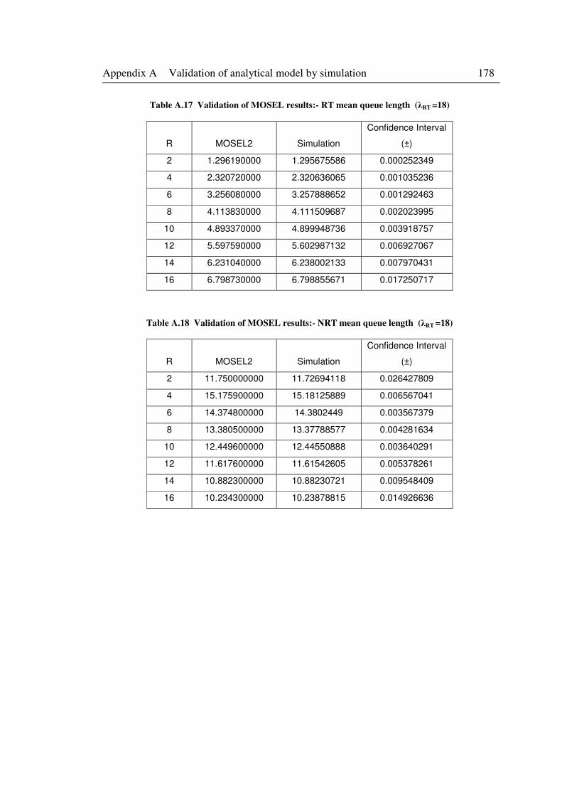
Appendix A Validation of analytical model by simulation 178
Table A.17 Validation of MOSEL results:- RT mean queue length (λRT =18)
R MOSEL2 Simulation
Confidence Interval
(±)
2 1.296190000 1.295675586 0.000252349
4 2.320720000 2.320636065 0.001035236
6 3.256080000 3.257888652 0.001292463
8 4.113830000 4.111509687 0.002023995
10 4.893370000 4.899948736 0.003918757
12 5.597590000 5.602987132 0.006927067
14 6.231040000 6.238002133 0.007970431
16 6.798730000 6.798855671 0.017250717
Table A.18 Validation of MOSEL results:- NRT mean queue length (λRT =18)
R MOSEL2 Simulation
Confidence Interval
(±)
2 11.750000000 11.72694118 0.026427809
4 15.175900000 15.18125889 0.006567041
6 14.374800000 14.3802449 0.003567379
8 13.380500000 13.37788577 0.004281634
10 12.449600000 12.44550888 0.003640291
12 11.617600000 11.61542605 0.005378261
14 10.882300000 10.88230721 0.009548409
16 10.234300000 10.23878815 0.014926636
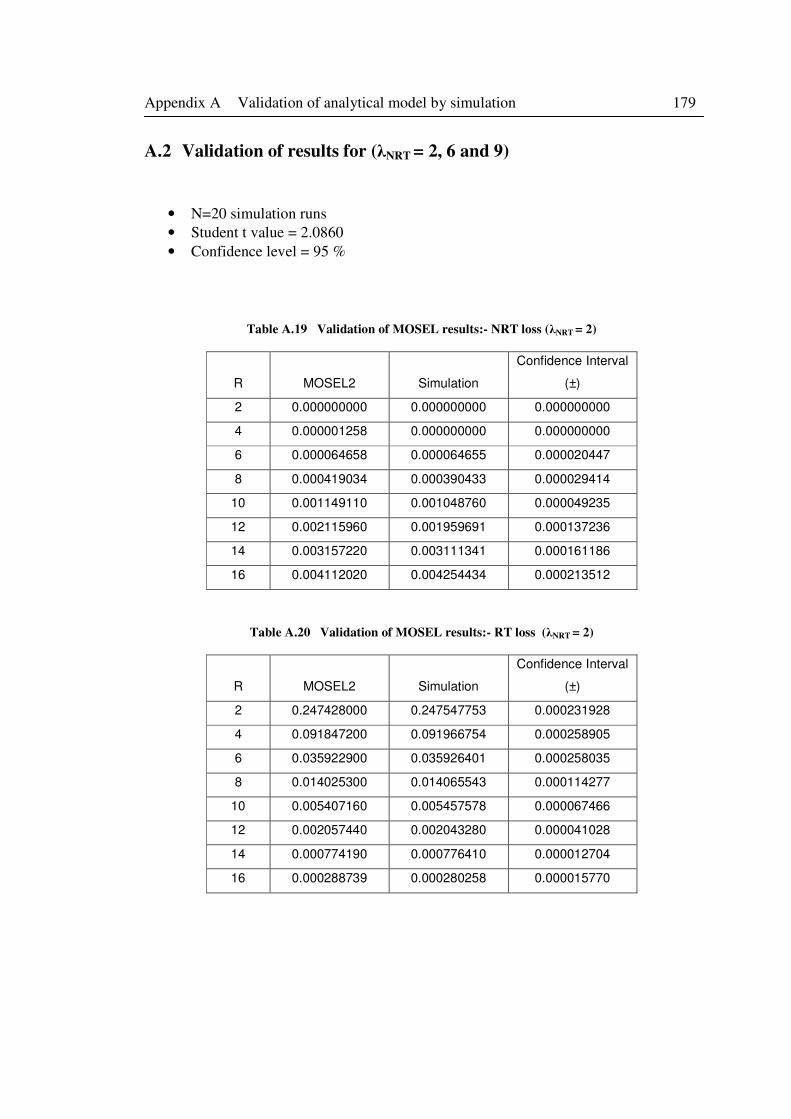
Appendix A Validation of analytical model by simulation 179
A.2 Validation of results for (λNRT = 2, 6 and 9)
• N=20 simulation runs
• Student t value = 2.0860
• Confidence level = 95 %
Table A.19 Validation of MOSEL results:- NRT loss (λNRT = 2)
R MOSEL2 Simulation
Confidence Interval
(±)
2 0.000000000 0.000000000 0.000000000
4 0.000001258 0.000000000 0.000000000
6 0.000064658 0.000064655 0.000020447
8 0.000419034 0.000390433 0.000029414
10 0.001149110 0.001048760 0.000049235
12 0.002115960 0.001959691 0.000137236
14 0.003157220 0.003111341 0.000161186
16 0.004112020 0.004254434 0.000213512
Table A.20 Validation of MOSEL results:- RT loss (λNRT = 2)
R MOSEL2 Simulation
Confidence Interval
(±)
2 0.247428000 0.247547753 0.000231928
4 0.091847200 0.091966754 0.000258905
6 0.035922900 0.035926401 0.000258035
8 0.014025300 0.014065543 0.000114277
10 0.005407160 0.005457578 0.000067466
12 0.002057440 0.002043280 0.000041028
14 0.000774190 0.000776410 0.000012704
16 0.000288739 0.000280258 0.000015770
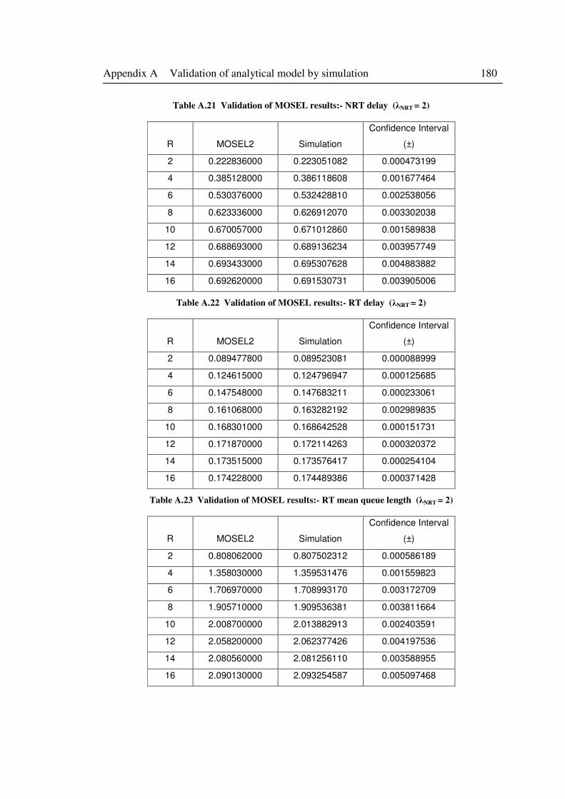
Appendix A Validation of analytical model by simulation 180
Table A.21 Validation of MOSEL results:- NRT delay (λNRT = 2)
R MOSEL2 Simulation
Confidence Interval
(±)
2 0.222836000 0.223051082 0.000473199
4 0.385128000 0.386118608 0.001677464
6 0.530376000 0.532428810 0.002538056
8 0.623336000 0.626912070 0.003302038
10 0.670057000 0.671012860 0.001589838
12 0.688693000 0.689136234 0.003957749
14 0.693433000 0.695307628 0.004883882
16 0.692620000 0.691530731 0.003905006
Table A.22 Validation of MOSEL results:- RT delay (λNRT = 2)
R MOSEL2 Simulation
Confidence Interval
(±)
2 0.089477800 0.089523081 0.000088999
4 0.124615000 0.124796947 0.000125685
6 0.147548000 0.147683211 0.000233061
8 0.161068000 0.163282192 0.002989835
10 0.168301000 0.168642528 0.000151731
12 0.171870000 0.172114263 0.000320372
14 0.173515000 0.173576417 0.000254104
16 0.174228000 0.174489386 0.000371428
Table A.23 Validation of MOSEL results:- RT mean queue length (λNRT = 2)
R MOSEL2 Simulation
Confidence Interval
(±)
2 0.808062000 0.807502312 0.000586189
4 1.358030000 1.359531476 0.001559823
6 1.706970000 1.708993170 0.003172709
8 1.905710000 1.909536381 0.003811664
10 2.008700000 2.013882913 0.002403591
12 2.058200000 2.062377426 0.004197536
14 2.080560000 2.081256110 0.003588955
16 2.090130000 2.093254587 0.005097468
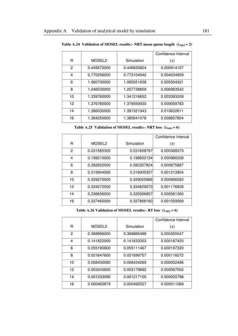
Appendix A Validation of analytical model by simulation 181
Table A.24 Validation of MOSEL results:- NRT mean queue length (λNRT = 2)
R MOSEL2 Simulation
Confidence Interval
(±)
2 0.445672000 0.446635824 0.000914157
4 0.770256000 0.773104942 0.004034859
6 1.060730000 1.065551838 0.005504321
8 1.246530000 1.257738859 0.006983542
10 1.339760000 1.341216652 0.003393209
12 1.376780000 1.379550930 0.009059783
14 1.386030000 1.391521943 0.010632611
16 1.384250000 1.385641078 0.008857804
Table A.25 Validation of MOSEL results:- NRT loss (λNRT = 6)
R MOSEL2 Simulation
Confidence Interval
(±)
2 0.031585300 0.031658797 0.000368373
4 0.199210000 0.198832134 0.000966208
6 0.282652000 0.282327824 0.000875887
8 0.315944000 0.316000357 0.001213804
10 0.329270000 0.329055966 0.000956583
12 0.334572000 0.334829270 0.001176828
14 0.336656000 0.335936857 0.000581360
16 0.337465000 0.337868160 0.001059069
Table A.26 Validation of MOSEL results:- RT loss (λNRT = 6)
R MOSEL2 Simulation
Confidence Interval
(±)
2 0.368896000 0.368866488 0.000355547
4 0.141822000 0.141633353 0.000187425
6 0.055190800 0.055111467 0.000197320
8 0.021647600 0.021699757 0.000116072
10 0.008430080 0.008434269 0.000052486
12 0.003243650 0.003179682 0.000067002
14 0.001233090 0.001217105 0.000020798
16 0.000463879 0.000495527 0.000011069
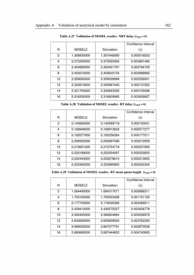
Appendix A Validation of analytical model by simulation 182
Table A.27 Validation of MOSEL results:- NRT delay (λNRT = 6)
R MOSEL2 Simulation
Confidence Interval
(±)
2 1.308830000 1.307446080 0.005518533
4 2.373350000 2.375925956 0.003891480
6 2.454580000 2.454431797 0.002794105
8 2.403510000 2.405603134 0.003988865
10 2.359060000 2.359539998 0.002556001
12 2.333910000 2.335987440 0.002131503
14 2.321700000 2.320843550 0.002105096
16 2.316250000 2.316605665 0.003009927
Table A.28 Validation of MOSEL results:- RT delay (λNRT = 6)
R MOSEL2 Simulation
Confidence Interval
(±)
2 0.140560000 0.140589718 0.000150031
4 0.169949000 0.169913628 0.000077277
6 0.192077000 0.192256264 0.000177011
8 0.206930000 0.206997498 0.000212009
10 0.215601000 0.215754719 0.000227905
12 0.220188000 0.220354097 0.000332820
14 0.222443000 0.222678610 0.000213693
16 0.223492000 0.223990893 0.000302324
Table A.29 Validation of MOSEL results:- RT mean queue length (λNRT = 6)
R MOSEL2 Simulation
Confidence Interval
(±)
2 1.064490000 1.064317671 0.000888311
4 1.750160000 1.750033488 0.001151120
6 2.177720000 2.178435396 0.002489011
8 2.429410000 2.430275227 0.003428778
10 2.565400000 2.566604864 0.003036979
12 2.633690000 2.635809583 0.003762200
14 2.666030000 2.667577791 0.002870538
16 2.680660000 2.687444602 0.004743903
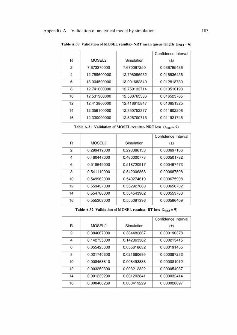
Appendix A Validation of analytical model by simulation 183
Table A.30 Validation of MOSEL results:- NRT mean queue length (λNRT = 6)
R MOSEL2 Simulation
Confidence Interval
(±)
2 7.673370000 7.670097250 0.036795436
4 12.789600000 12.798096982 0.018536436
6 13.004500000 13.001682840 0.012818730
8 12.741600000 12.750133714 0.013510193
10 12.531900000 12.530765336 0.016523785
12 12.413800000 12.418615847 0.010651325
14 12.356100000 12.350752377 0.011602208
16 12.330000000 12.325700715 0.011921745
Table A.31 Validation of MOSEL results:- NRT loss (λNRT = 9)
R MOSEL2 Simulation
Confidence Interval
(±)
2 0.299419000 0.298386133 0.000697106
4 0.460447000 0.460000773 0.000501782
6 0.518649000 0.518720917 0.000497473
8 0.541110000 0.542006868 0.000687508
10 0.549962000 0.549274619 0.000675998
12 0.553437000 0.552927660 0.000656702
14 0.554786000 0.554543902 0.000553783
16 0.555303000 0.555091396 0.000586409
Table A.32 Validation of MOSEL results:- RT loss (λNRT = 9)
R MOSEL2 Simulation
Confidence Interval
(±)
2 0.384667000 0.384482867 0.000190378
4 0.142735000 0.142363362 0.000215415
6 0.055425600 0.055618632 0.000191455
8 0.021740600 0.021660695 0.000087232
10 0.008468810 0.008493836 0.000081912
12 0.003259390 0.003212322 0.000054937
14 0.001239290 0.001203841 0.000032414
16 0.000466269 0.000419229 0.000028697
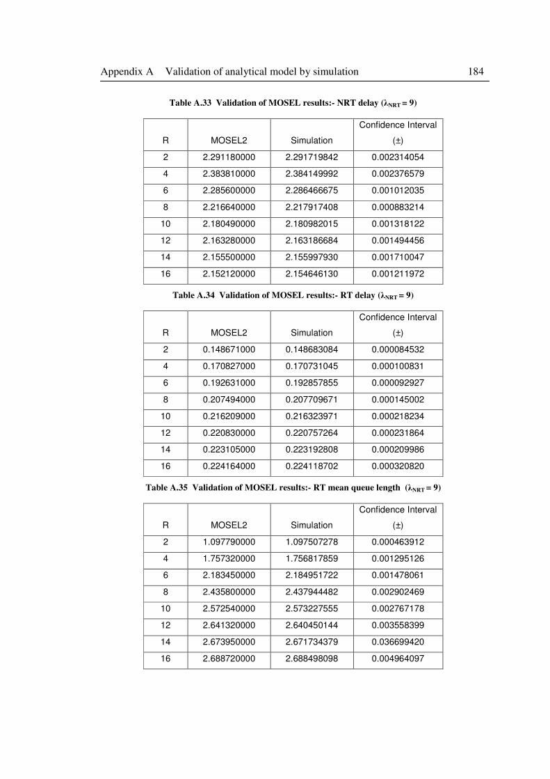
Appendix A Validation of analytical model by simulation 184
Table A.33 Validation of MOSEL results:- NRT delay (λNRT = 9)
R MOSEL2 Simulation
Confidence Interval
(±)
2 2.291180000 2.291719842 0.002314054
4 2.383810000 2.384149992 0.002376579
6 2.285600000 2.286466675 0.001012035
8 2.216640000 2.217917408 0.000883214
10 2.180490000 2.180982015 0.001318122
12 2.163280000 2.163186684 0.001494456
14 2.155500000 2.155997930 0.001710047
16 2.152120000 2.154646130 0.001211972
Table A.34 Validation of MOSEL results:- RT delay (λNRT = 9)
R MOSEL2 Simulation
Confidence Interval
(±)
2 0.148671000 0.148683084 0.000084532
4 0.170827000 0.170731045 0.000100831
6 0.192631000 0.192857855 0.000092927
8 0.207494000 0.207709671 0.000145002
10 0.216209000 0.216323971 0.000218234
12 0.220830000 0.220757264 0.000231864
14 0.223105000 0.223192808 0.000209986
16 0.224164000 0.224118702 0.000320820
Table A.35 Validation of MOSEL results:- RT mean queue length (λNRT = 9)
R MOSEL2 Simulation
Confidence Interval
(±)
2 1.097790000 1.097507278 0.000463912
4 1.757320000 1.756817859 0.001295126
6 2.183450000 2.184951722 0.001478061
8 2.435800000 2.437944482 0.002902469
10 2.572540000 2.573227555 0.002767178
12 2.641320000 2.640450144 0.003558399
14 2.673950000 2.671734379 0.036699420
16 2.688720000 2.688498098 0.004964097
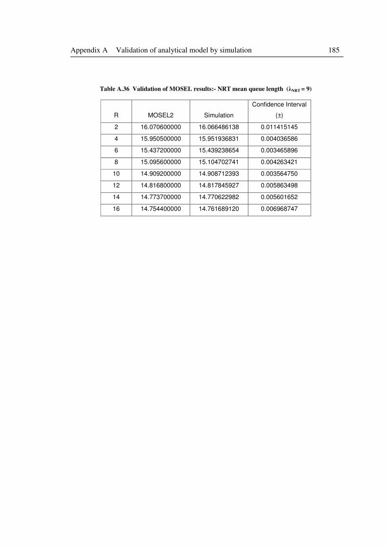
Appendix A Validation of analytical model by simulation 185
Table A.36 Validation of MOSEL results:- NRT mean queue length (λNRT = 9)
R MOSEL2 Simulation
Confidence Interval
(±)
2 16.070600000 16.066486138 0.011415145
4 15.950500000 15.951936831 0.004036586
6 15.437200000 15.439238654 0.003465896
8 15.095600000 15.104702741 0.004263421
10 14.909200000 14.908712393 0.003564750
12 14.816800000 14.817845927 0.005863498
14 14.773700000 14.770622982 0.005601652
16 14.754400000 14.761689120 0.006968747

Appendix B HSDPA model development in OPNET 186
Appendix B
HSDPA Model Development in
OPNET
For the purpose of end-to-end evaluation of our proposed buffer management schemes, a
custom system level HSDPA simulator was developed using the network modelling
simulation tool, OPNET modeler. OPNET has a clear and simple hierarchical network
modelling paradigm where behaviour of individual objects can be modelled at process
level and then interconnected to form devices at the node level. Node level devices can
be interconnected using links to form networks at the network level. Multiple network
scenarios can be organized into a project to compare designs or configurations. Proto-
cols and other processes are modelled using finite state machines (FSM). Any required
behaviour can be simulated with C/C++ logic in the FSM states and transitions, and the
user has control over the level of detail that can be represented. Our simulator is built to
realistically model the HSDPA data flow mechanisms described in section 3.7 of
chapter 3 with as much detail as possible in order to facilitate end-to-end evaluation.
Although built for buffer management evaluation, the simulator can be customized for
other HSDPA network level performance studies as well.
B.1 Design approach
The OPNET hierarchical network modelling paradigm was employed in developing the
HSDPA simulator. Thus, a set of node objects, which provide the building blocks for
various HSDPA network configurations for the end-to-end study were designed and
developed. These were organized into a collection of HSDPA simulation model library
consisting of:
Appendix B HSDPA model development in OPNET 187
• Traffic source nodes generating multiple flows.
• UTRAN node with detailed RNC and Node B models.
• UE receiver node models.
• Unidirectional and bi-directional links.
• Packet formats as per the various protocols implemented.
Another design approach employed in our simulator involves embedding a central
synchronous event controller which periodically generates timed control signals to
remotely trigger modules that are required to update their states or execute a task at
regular intervals. This central controller is known as the TTI manager and is imple-
mented in the UTRAN node model. The TTI manager operates with granularity of
HSDPA TTI of 2ms, sending remote triggers every TTI to each UE to update its location
and SINR. It also sends triggers to the Node B module to enable credit allocation update
and inter-TTI packet scheduling; and to the RNC module to provide HS-DSCH Frame
Protocol inter-frame alignment. The asynchronous aspect allows for modelling non-
periodic or irregular events such as source traffic generation or response to packet
arrivals at the node entities, which are generally independent of the HSDPA TTI timing.
The control of asynchronous events are of course distributed amongst the individual
modules rather than centralized like the synchronous ones governed by the TTI manager.
B.2 Traffic source node implementation
The traffic source node is designed to generate and transmit independent RT and NRT
traffic flows to an individual receiver in the HSDPA cell. It consists of two modules with
their process models depicted in Figure B.1. RT_source can be configured to generate
ON/OFF VoIP packets or other RT traffic patterns with different packet sizes and
various packet inter-arrival distributions e.g. exponential, deterministic, etc. The
ss_packet_generate() function, which is invoked by the PACKET_GENERATE inter-
rupt is adapted from the standard OPNET simple_source process model with additional
code segments implemented to enable a wider range of RT traffic generation patterns.
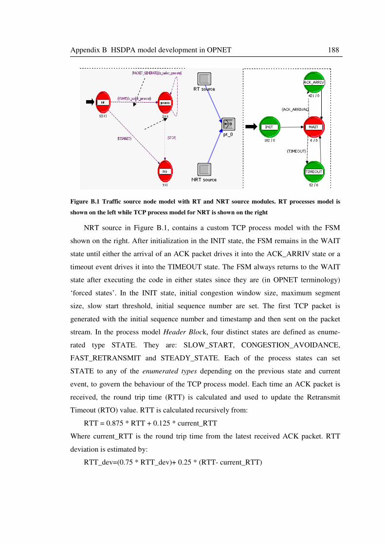
Appendix B HSDPA model development in OPNET 188
Figure B.1 Traffic source node model with RT and NRT source modules. RT processes model is
shown on the left while TCP process model for NRT is shown on the right
NRT source in Figure B.1, contains a custom TCP process model with the FSM
shown on the right. After initialization in the INIT state, the FSM remains in the WAIT
state until either the arrival of an ACK packet drives it into the ACK_ARRIV state or a
timeout event drives it into the TIMEOUT state. The FSM always returns to the WAIT
state after executing the code in either states since they are (in OPNET terminology)
‘forced states’. In the INIT state, initial congestion window size, maximum segment
size, slow start threshold, initial sequence number are set. The first TCP packet is
generated with the initial sequence number and timestamp and then sent on the packet
stream. In the process model Header Block, four distinct states are defined as enume-
rated type STATE. They are: SLOW_START, CONGESTION_AVOIDANCE,
FAST_RETRANSMIT and STEADY_STATE. Each of the process states can set
STATE to any of the enumerated types depending on the previous state and current
event, to govern the behaviour of the TCP process model. Each time an ACK packet is
received, the round trip time (RTT) is calculated and used to update the Retransmit
Timeout (RTO) value. RTT is calculated recursively from:
RTT = 0.875 * RTT + 0.125 * current_RTT
Where current_RTT is the round trip time from the latest received ACK packet. RTT
deviation is estimated by:
RTT_dev=(0.75 * RTT_dev)+ 0.25 * (RTT- current_RTT)
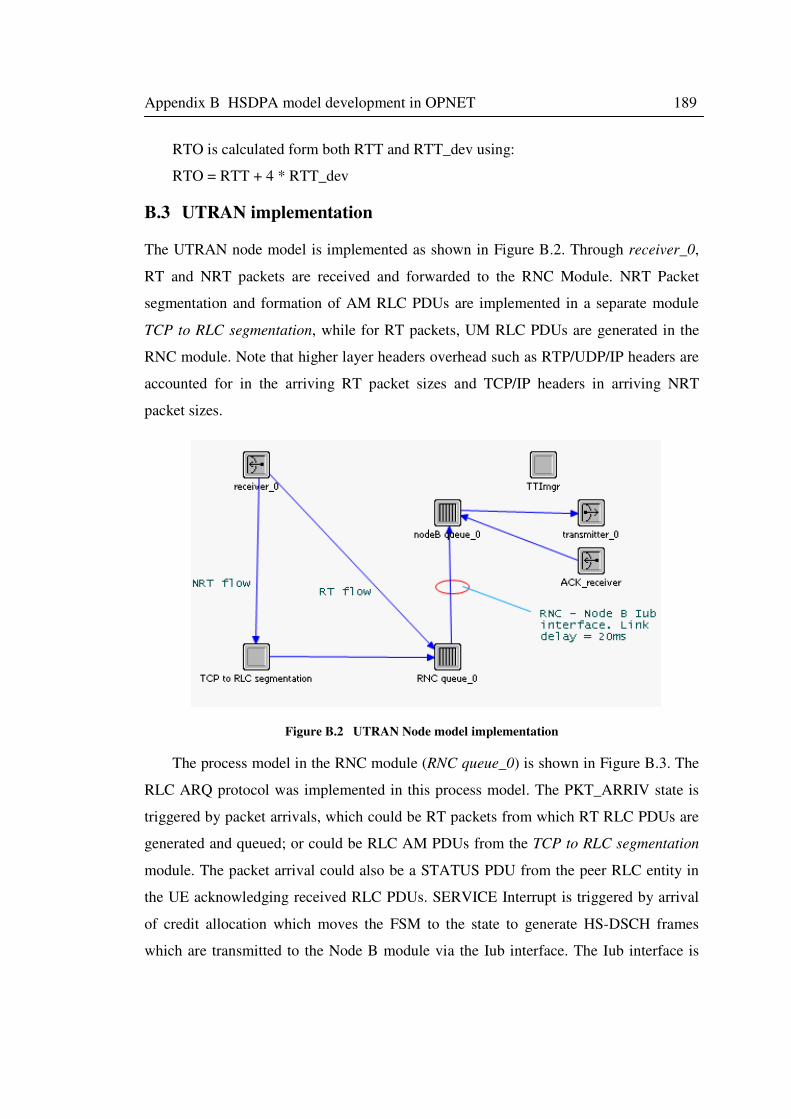
Appendix B HSDPA model development in OPNET 189
RTO is calculated form both RTT and RTT_dev using:
RTO = RTT + 4 * RTT_dev
B.3 UTRAN implementation
The UTRAN node model is implemented as shown in Figure B.2. Through receiver_0,
RT and NRT packets are received and forwarded to the RNC Module. NRT Packet
segmentation and formation of AM RLC PDUs are implemented in a separate module
TCP to RLC segmentation, while for RT packets, UM RLC PDUs are generated in the
RNC module. Note that higher layer headers overhead such as RTP/UDP/IP headers are
accounted for in the arriving RT packet sizes and TCP/IP headers in arriving NRT
packet sizes.
Figure B.2 UTRAN Node model implementation
The process model in the RNC module (RNC queue_0) is shown in Figure B.3. The
RLC ARQ protocol was implemented in this process model. The PKT_ARRIV state is
triggered by packet arrivals, which could be RT packets from which RT RLC PDUs are
generated and queued; or could be RLC AM PDUs from the TCP to RLC segmentation
module. The packet arrival could also be a STATUS PDU from the peer RLC entity in
the UE acknowledging received RLC PDUs. SERVICE Interrupt is triggered by arrival
of credit allocation which moves the FSM to the state to generate HS-DSCH frames
which are transmitted to the Node B module via the Iub interface. The Iub interface is
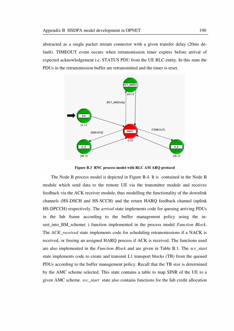
Appendix B HSDPA model development in OPNET 190
abstracted as a single packet stream connector with a given transfer delay (20ms de-
fault). TIMEOUT event occurs when retransmission timer expires before arrival of
expected acknowledgement i.e. STATUS PDU from the UE RLC entity. In this state the
PDUs in the retransmission buffer are retransmitted and the timer is reset.
Figure B.3 RNC process model with RLC AM ARQ protocol
The Node B process model is depicted in Figure B.4. It is contained in the Node B
module which send data to the remote UE via the transmitter module and receives
feedback via the ACK receiver module, thus modelling the functionality of the downlink
channels (HS-DSCH and HS-SCCH) and the return HARQ feedback channel (uplink
HS-DPCCH) respectively. The arrival state implements code for queuing arriving PDUs
in the Iub frame according to the buffer management policy using the in-
sert_into_BM_scheme( ) function implemented in the process model Function Block.
The ACK_received state implements code for scheduling retransmissions if a NACK is
received, or freeing an assigned HARQ process if ACK is received. The functions used
are also implemented in the Function Block and are given in Table B.1. The scv_start
state implements code to create and transmit L1 transport blocks (TB) from the queued
PDUs according to the buffer management policy. Recall that the TB size is determined
by the AMC scheme selected. This state contains a table to map SINR of the UE to a
given AMC scheme. svc_start state also contains functions for the Iub credit allocation
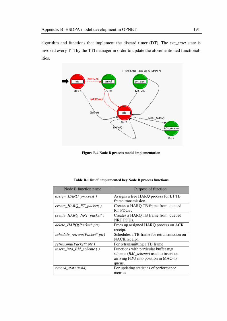
Appendix B HSDPA model development in OPNET 191
algorithm and functions that implement the discard timer (DT). The svc_start state is
invoked every TTI by the TTI manager in order to update the aforementioned functional-
ities.
Figure B.4 Node B process model implementation
Table B.1 list of implemented key Node B process functions
Node B function name Purpose of function
assign_HARQ_process( ) Assigns a free HARQ process for L1 TB
frame transmission.
create_HARQ_RT_packet( ) Creates a HARQ TB frame from queued
RT PDUs .
create_HARQ_NRT_packet( ) Creates a HARQ TB frame from queued
NRT PDUs.
delete_HARQ(Packet* ptr) Frees up assigned HARQ process on ACK
receipt.
schedule_retrans(Packet* ptr) Schedules a TB frame for retransmission on
NACK receipt.
retransmit(Packet* ptr ) For retransmitting a TB frame
insert_into_BM_scheme ( ) Functions with particular buffer mgt.
scheme (BM_scheme) used to insert an
arriving PDU into position in MAC-hs
queue.
record_stats (void) For updating statistics of performance
metrics
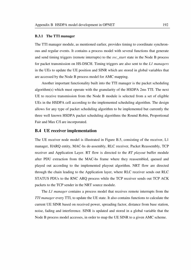
Appendix B HSDPA model development in OPNET 192
B.3.1 The TTI manager
The TTI manager module, as mentioned earlier, provides timing to coordinate synchron-
ous and regular events. It contains a process model with several functions that generate
and send timing triggers (remote interrupts) to the svc_start state in the Node B process
for packet transmission on HS-DSCH. Timing triggers are also sent to the L1 managers
in the UEs to update the UE position and SINR which are stored in global variables that
are accessed by the Node B process model for AMC mapping.
Another important functionality built into the TTI manager is the packet scheduling
algorithm(s) which must operate with the granularity of the HSDPA 2ms TTI. The next
UE to receive transmission from the Node B module is selected from a set of eligible
UEs in the HSDPA cell according to the implemented scheduling algorithm. The design
allows for any type of packet scheduling algorithm to be implemented but currently the
three well known HSDPA packet scheduling algorithms the Round Robin, Proportional
Fair and Max C/I are incorporated.
B.4 UE receiver implementation
The UE receiver node model is illustrated in Figure B.5, consisting of the receiver, L1
manager, HARQ entity, MAC-hs de-assembly, RLC receiver, Packet Reassembly, TCP
receiver and Application Layer. RT flow is directed to the RT playout buffer module
after PDU extraction from the MAC-hs frame where they reassembled, queued and
played out according to the implemented playout algorithm. NRT flow are directed
through the chain leading to the Application layer, where RLC receiver sends out RLC
STATUS PDUs to the RNC ARQ process while the TCP receiver sends out TCP ACK
packets to the TCP sender in the NRT source module.
The L1 manager contains a process model that receives remote interrupts from the
TTI manager every TTI, to update the UE state. It also contains functions to calculate the
current UE SINR based on received power, spreading factor, distance from base station,
noise, fading and interference. SINR is updated and stored in a global variable that the
Node B process model accesses, in order to map the UE SINR to a given AMC scheme.
Appendix B HSDPA model development in OPNET 193
Figure B.5 UE receiver node model implementation