Embed Size (px)
Citation preview
Quantified Boolean Formula (QBF) Reasoning
Bart Selman, Carla Gomes, Ashish Sabharwal
Cornell University
Feb 13, 2007
Tutorial forDr. Charles Holland and Dr. Tom Wagner
2
Tutorial Roadmap
1. Automated reasoning– The complexity challenge– State of the art in Boolean reasoning
2. SAT-based reasoning– Boolean logic– Search space, worst-case complexity– Hardness profiles, scaling in practice– Modeling problems as SAT
• Example domain: planning
3. QBF reasoning (extends SAT)– A new range of applications– Two motivating examples
• network planning, logistics planning
– Quantified Boolean logic– Modeling problems as QBF– Search space, worst-case complexity– Scaling in practice
4. High-Performance QBF reasoning– Key research advances– The technology behind QBF– A. New modeling techniques– B. Learning while reasoning– C. Structure discovery– Experimental Results
5. Summary
3
Tutorial Roadmap
1. Automated reasoning The complexity challenge– State of the art in Boolean reasoning
2. SAT-based reasoning– Boolean logic– Search space, worst-case complexity– Hardness profiles, scaling in practice– Modeling problems as SAT
• Example domain: planning
3. QBF reasoning (extends SAT)– A new range of applications– Two motivating examples
• network planning, logistics planning
– Quantified Boolean logic– Modeling problems as QBF– Search space, worst-case complexity– Scaling in practice
4. High-Performance QBF reasoning– Key research advances– The technology behind QBF– A. New modeling techniques– B. Learning while reasoning– C. Structure discovery– Experimental Results
5. Summary
4
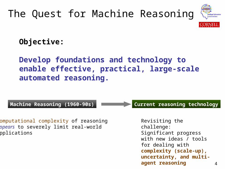
The Quest for Machine Reasoning
Objective:
Develop foundations and technology to enable effective, practical, large-scale automated reasoning.
Computational complexity of reasoning appears to severely limit real-world applications
Current reasoning technology
Revisiting the challenge:Significant progress with new ideas / tools for dealing with complexity (scale-up), uncertainty, and multi-agent reasoning
Machine Reasoning (1960-90s)
5
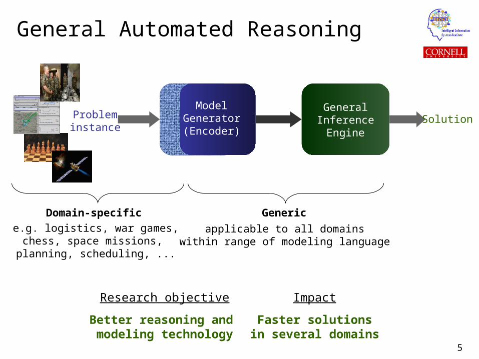
General Automated Reasoning
GeneralInferenceEngine
Solution
Domain-specific
Probleminstance
applicable to all domainswithin range of modeling language
ModelGenerator(Encoder)
Research objective
Better reasoning and modeling technology
Impact
Faster solutionsin several domains
e.g. logistics, war games,chess, space missions, planning, scheduling, ...
Generic
6
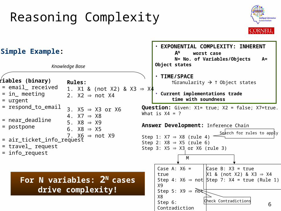
• EXPONENTIAL COMPLEXITY: INHERENT AN worst case N= No. of Variables/Objects A= Object states
• TIME/SPACE Granularity Object states
• Current implementations trade time with soundness
Question: Given: X1= true; X2 = false; X7=true. What is X4 = ?
Answer Development: Inference Chain
Step 1: X7 X8 (rule 4)Step 2: X8 X5 (rule 6)Step 3: X5 X3 or X6 (rule 3)
Case A: X6 = trueStep 4: X6 not X9Step 5: X9 not X8Step 6: Contradiction Backtrack to M
Case B: X3 = trueX1 & (not X2) & X3 X4Step 7: X4 = true (Rule 1)
M
Search for rules to apply
Check Contradictions
For N variables: 2N cases drive complexity!
Simple Example:
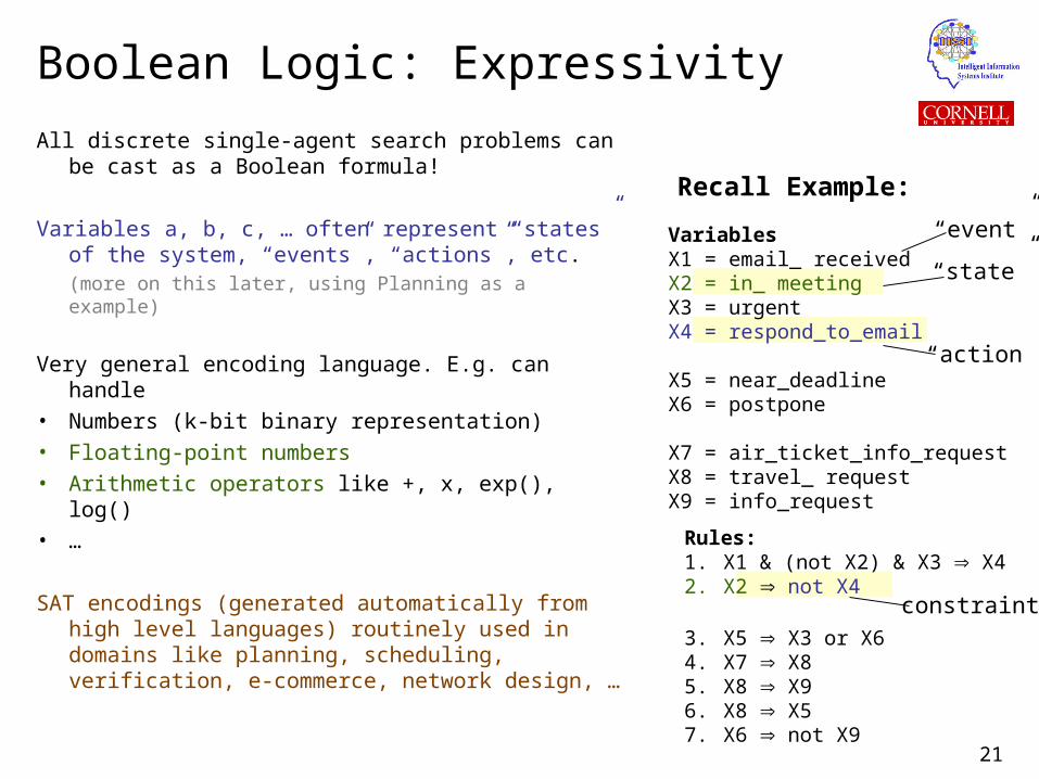
Variables (binary)X1 = email_ receivedX2 = in_ meetingX3 = urgentX4 = respond_to_email
X5 = near_deadlineX6 = postpone
X7 = air_ticket_info_requestX8 = travel_ requestX9 = info_request
Rules:1. X1 & (not X2) & X3 X42. X2 not X4
3. X5 X3 or X64. X7 X85. X8 X96. X8 X57. X6 not X9
Knowledge Base
Reasoning Complexity
7
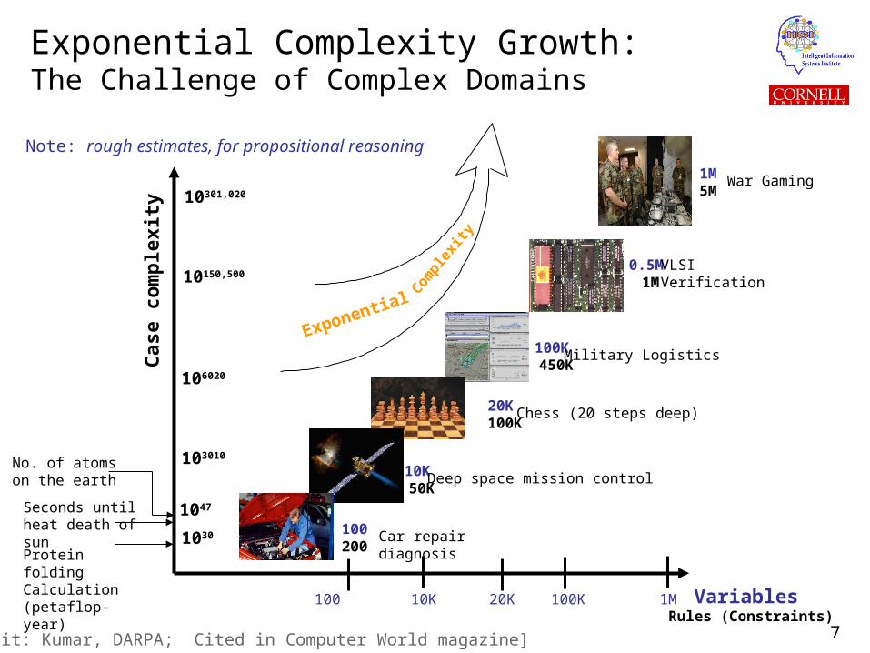
Exponential Complexity Growth: The Challenge of Complex Domains
100 200
10K 50K
20K 100K
0.5M 1M
1M5M
Variables
1030
10301,020
10150,500
106020
103010
Cas
e co
mp
lexi
ty
Car repair diagnosis
Deep space mission control
Chess (20 steps deep)
VLSIVerification
War Gaming
100K 450K
Military Logistics
Seconds until heat death of sun
Protein foldingCalculation (petaflop-year)
No. of atomson the earth
1047
100 10K 20K 100K 1MRules (Constraints)
Exponential
Compl
exity
Note: rough estimates, for propositional reasoning
[Credit: Kumar, DARPA; Cited in Computer World magazine]
8
Tutorial Roadmap
1. Automated reasoning The complexity challenge State of the art in Boolean reasoning
2. SAT-based reasoning– Boolean logic– Search space, worst-case complexity– Hardness profiles, scaling in practice– Modeling problems as SAT
• Example domain: planning
3. QBF reasoning (extends SAT)– A new range of applications– Two motivating examples
• network planning, logistics planning
– Quantified Boolean logic– Modeling problems as QBF– Search space, worst-case complexity– Scaling in practice
4. High-Performance QBF reasoning– Key research advances– The technology behind QBF– A. New modeling techniques– B. Learning while reasoning– C. Structure discovery– Experimental Results
5. Summary
9
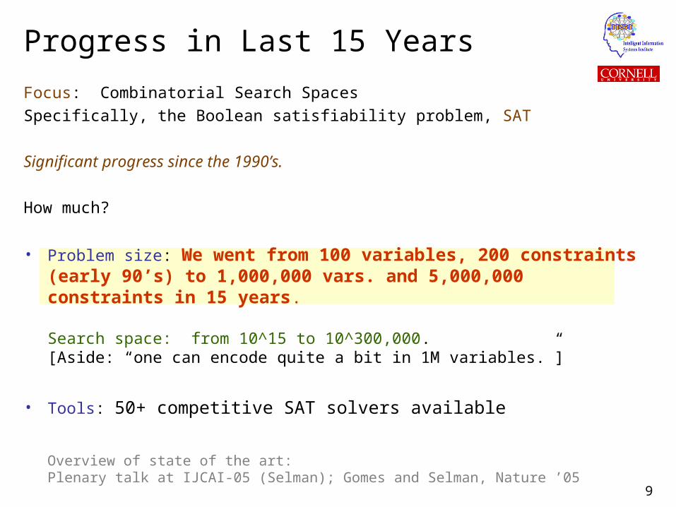
Focus: Combinatorial Search Spaces
Specifically, the Boolean satisfiability problem, SAT
Significant progress since the 1990’s.
How much?
• Problem size: We went from 100 variables, 200 constraints (early 90’s) to 1,000,000 vars. and 5,000,000 constraints in 15 years.
Search space: from 10^15 to 10^300,000.[Aside: “one can encode quite a bit in 1M variables.”]
• Tools: 50+ competitive SAT solvers available
Overview of state of the art: Plenary talk at IJCAI-05 (Selman); Gomes and Selman, Nature ’05
Progress in Last 15 Years
10
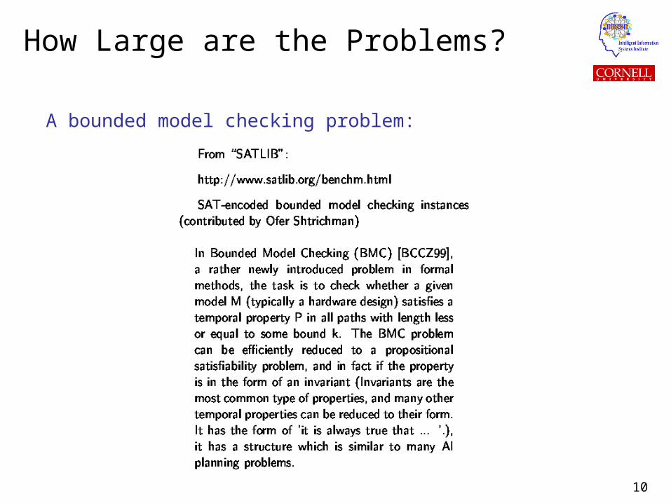
How Large are the Problems?
A bounded model checking problem:
11
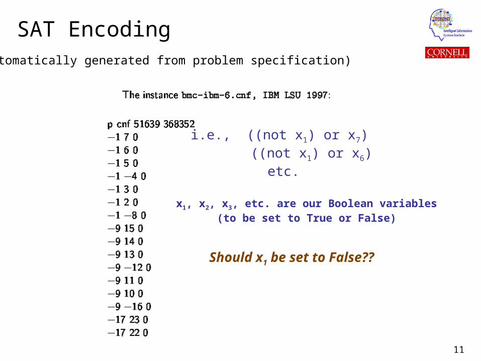
i.e., ((not x1) or x7) ((not x1) or x6)
etc.
x1, x2, x3, etc. are our Boolean variables(to be set to True or False)
Should x1 be set to False??
SAT Encoding(automatically generated from problem specification)
12
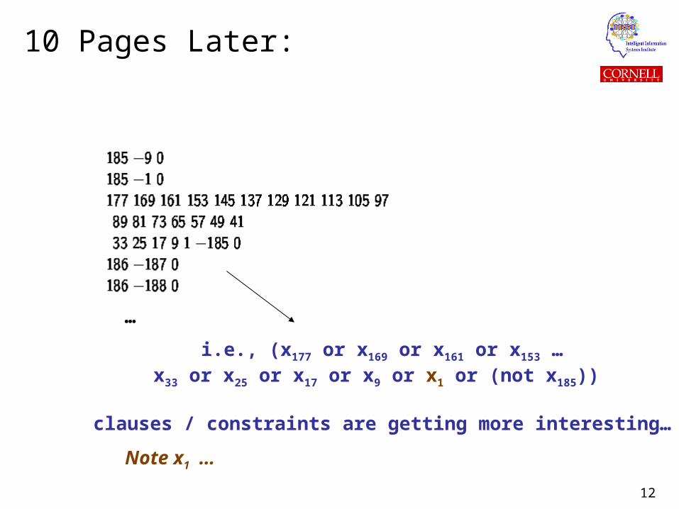
i.e., (x177 or x169 or x161 or x153 …x33 or x25 or x17 or x9 or x1 or (not x185))
clauses / constraints are getting more interesting…
…
Note x1 …
10 Pages Later:
13
…
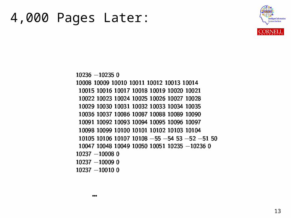
4,000 Pages Later:
14
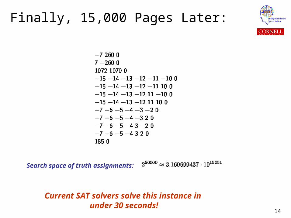
Current SAT solvers solve this instance in under 30 seconds!
Search space of truth assignments:
Finally, 15,000 Pages Later:
15
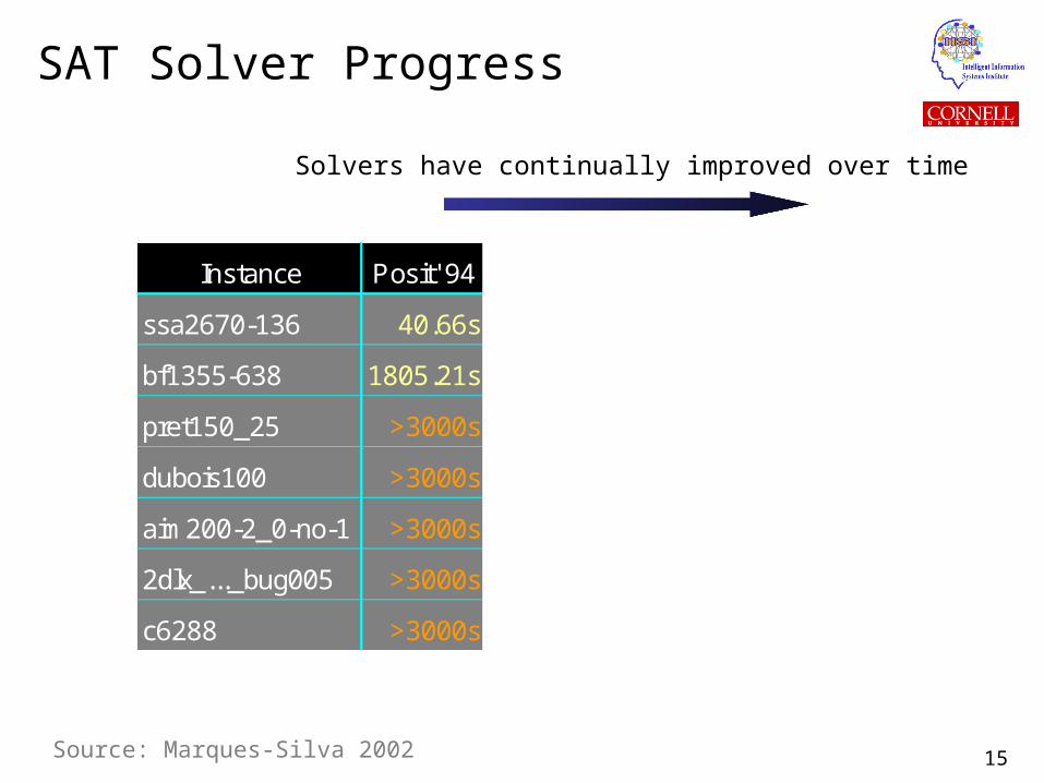
SAT Solver Progress
Instance Posit' 94 Grasp' 96 Sato' 98 Chaff' 01
ssa2670-136 40.66s 1.20s 0.95s 0.02s
bf1355-638 1805.21s 0.11s 0.04s 0.01s
pret150_25 >3000s 0.21s 0.09s 0.01s
dubois100 >3000s 11.85s 0.08s 0.01s
aim200-2_0-no-1 >3000s 0.01s < 0.01s < 0.01s
2dlx_..._bug005 >3000s >3000s >3000s 2.90s
c6288 >3000s >3000s >3000s >3000s
Source: Marques-Silva 2002
Solvers have continually improved over time
16
How do SAT Solvers Keep Improving?
From academically interesting to practically relevant.
We now have regular SAT solver competitions.
(Germany ’89, Dimacs ’93, China ’96, SAT-02, SAT-03, SAT-04, SAT-05, SAT-06)
E.g. at SAT-2006 (Seattle, Aug ’06):
• 35+ solvers submitted, most of them open source
• 500+ industrial benchmarks
• 50,000+ benchmark instances available on the www
This constant improvement in SAT solvers is the key to making, e.g.,SAT-based planning very successful.
17
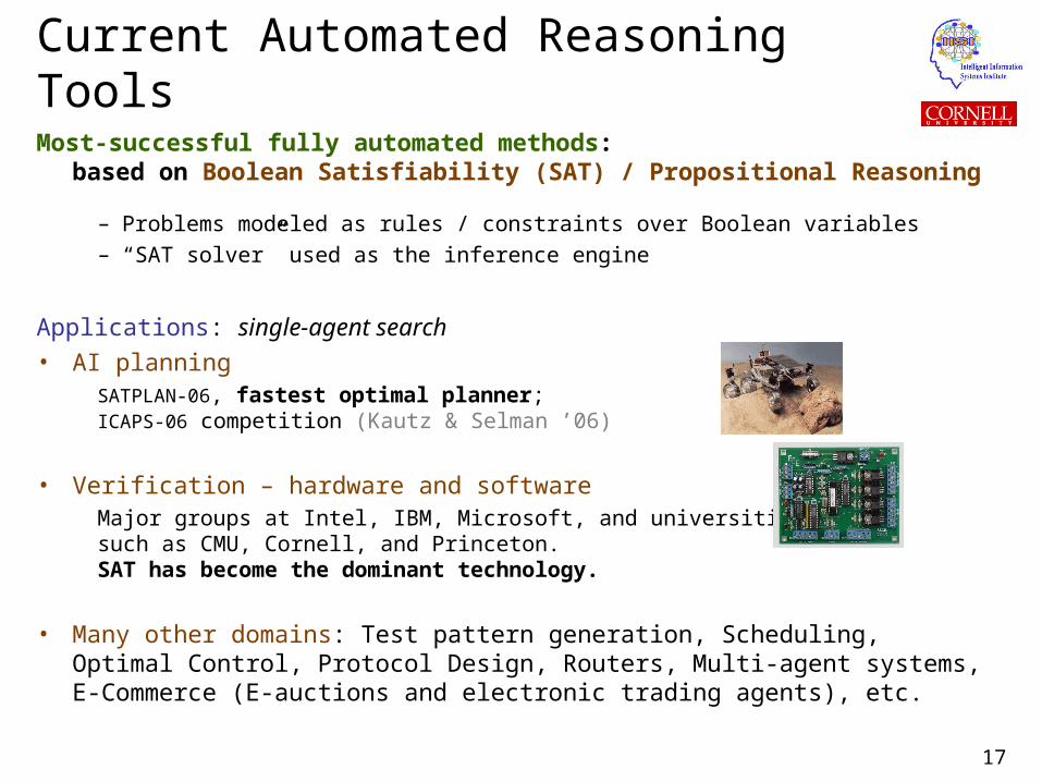
Current Automated Reasoning Tools
Most-successful fully automated methods: based on Boolean Satisfiability (SAT) / Propositional Reasoning
– Problems modeled as rules / constraints over Boolean variables– “SAT solver” used as the inference engine
Applications: single-agent search
• AI planning SATPLAN-06, fastest optimal planner; ICAPS-06 competition (Kautz & Selman ’06)
• Verification – hardware and softwareMajor groups at Intel, IBM, Microsoft, and universitiessuch as CMU, Cornell, and Princeton.SAT has become the dominant technology.
• Many other domains: Test pattern generation, Scheduling,Optimal Control, Protocol Design, Routers, Multi-agent systems,E-Commerce (E-auctions and electronic trading agents), etc.
18
Tutorial Roadmap
Automated reasoning The complexity challenge State of the art in Boolean reasoning
2. SAT-based reasoning Boolean logic– Search space, worst-case complexity– Hardness profiles, scaling in practice– Modeling problems as SAT
• Example domain: planning
3. QBF reasoning (extends SAT)– A new range of applications– Two motivating examples
• network planning, logistics planning
– Quantified Boolean logic– Modeling problems as QBF– Search space, worst-case complexity– Scaling in practice
4. High-Performance QBF reasoning– Key research advances– The technology behind QBF– A. New modeling techniques– B. Learning while reasoning– C. Structure discovery– Experimental Results
5. Summary
19
Boolean Logic
Defined over Boolean (binary) variables a, b, c, …
Each of these can be True (1) or False (0)
Variables connected together with logic operators: and, or, not (denoted )
E.g. (a or b) is True iff at least one of a and b is True
((c and d)) or f) is True iff either c is True and d is False, or f is True
Fact: All other Boolean logic operators can be expressed with and, or, not E.g. (a b) same as (a or b)
Boolean formula, e.g. F = (a or b) and (a and (b or c))
(Truth) Assignment: any setting of the variables to True or False
Satisfying assignment: assignment where the formula evaluates to True
20
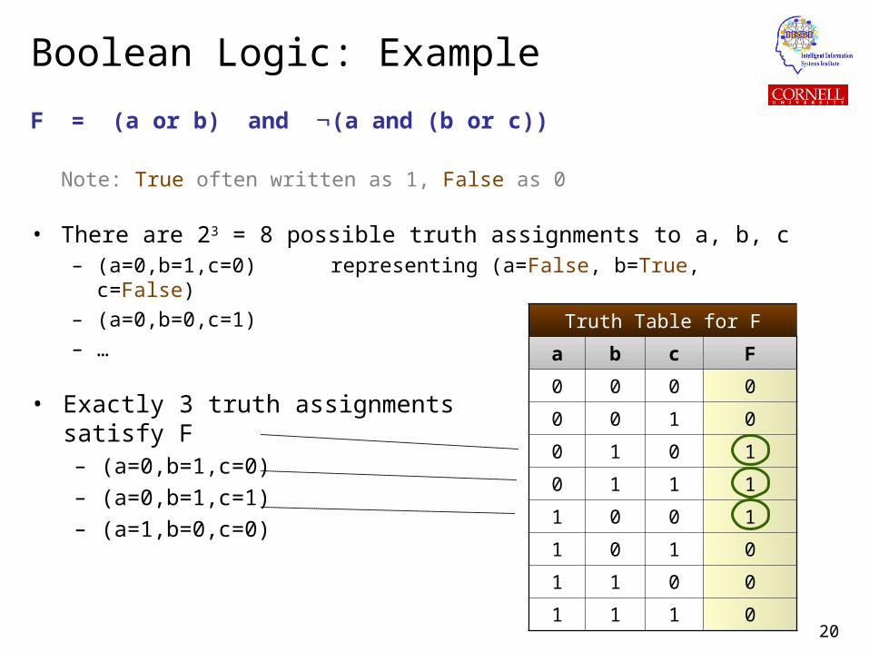
Boolean Logic: Example
F = (a or b) and (a and (b or c))
Note: True often written as 1, False as 0
• There are 23 = 8 possible truth assignments to a, b, c– (a=0,b=1,c=0) representing (a=False, b=True, c=False)
– (a=0,b=0,c=1)
– …Truth Table for F
a b c F
0 0 0 0
0 0 1 0
0 1 0 1
0 1 1 1
1 0 0 1
1 0 1 0
1 1 0 0
1 1 1 0
• Exactly 3 truth assignments satisfy F– (a=0,b=1,c=0)
– (a=0,b=1,c=1)
– (a=1,b=0,c=0)
21
Rules:1. X1 & (not X2) & X3 X42. X2 not X4
3. X5 X3 or X64. X7 X85. X8 X96. X8 X57. X6 not X9
VariablesX1 = email_ receivedX2 = in_ meetingX3 = urgentX4 = respond_to_email
X5 = near_deadlineX6 = postpone
X7 = air_ticket_info_requestX8 = travel_ requestX9 = info_request
Boolean Logic: Expressivity
All discrete single-agent search problems can be cast as a Boolean formula!
Variables a, b, c, … often represent “states” of the system, “events”, “actions”, etc.(more on this later, using Planning as a example)
Very general encoding language. E.g. can handle
• Numbers (k-bit binary representation)
• Floating-point numbers
• Arithmetic operators like +, x, exp(), log()
• …
SAT encodings (generated automatically from high level languages) routinely used in domains like planning, scheduling, verification, e-commerce, network design, …
Recall Example:
“state”
“action”
constraint
“event”
22
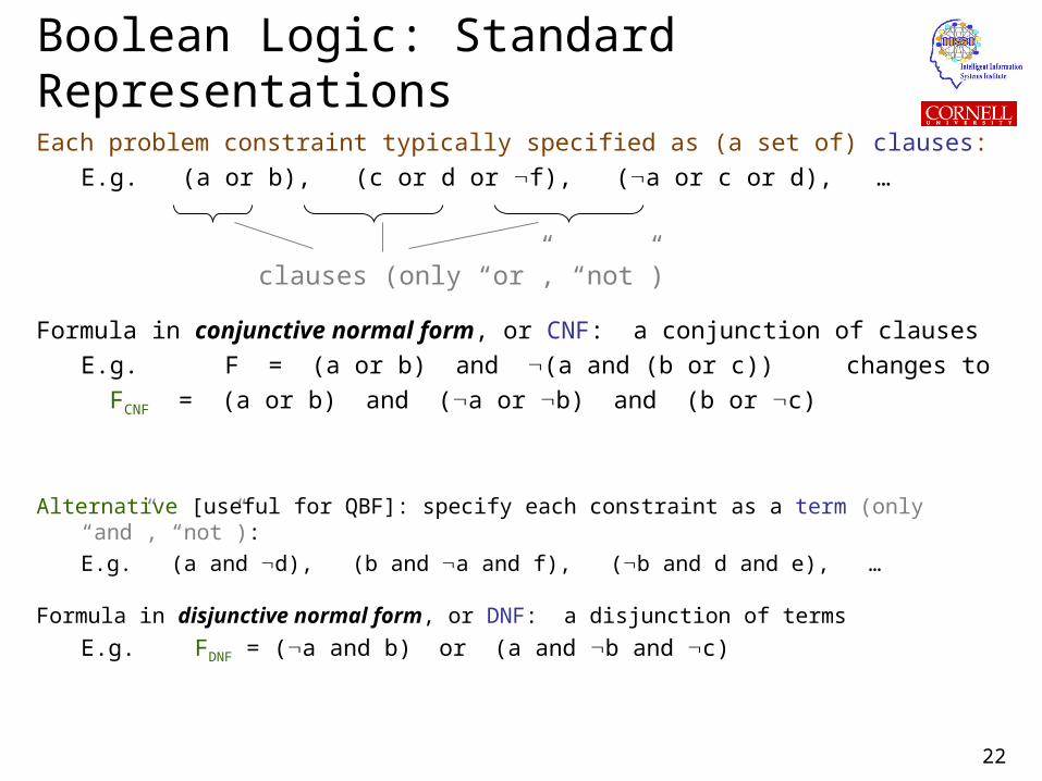
Boolean Logic: Standard Representations
Each problem constraint typically specified as (a set of) clauses:
E.g. (a or b), (c or d or f), (a or c or d), …
Formula in conjunctive normal form, or CNF: a conjunction of clauses
E.g. F = (a or b) and (a and (b or c)) changes to
FCNF = (a or b) and (a or b) and (b or c)
Alternative [useful for QBF]: specify each constraint as a term (only “and”, “not”):
E.g. (a and d), (b and a and f), (b and d and e), …
Formula in disjunctive normal form, or DNF: a disjunction of terms
E.g. FDNF = (a and b) or (a and b and c)
clauses (only “or”, “not”)
23
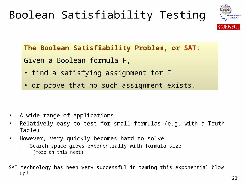
Boolean Satisfiability Testing
• A wide range of applications• Relatively easy to test for small formulas (e.g. with a Truth Table)• However, very quickly becomes hard to solve
– Search space grows exponentially with formula size (more on this next)
SAT technology has been very successful in taming this exponential blow up!
The Boolean Satisfiability Problem, or SAT:
Given a Boolean formula F,
• find a satisfying assignment for F
• or prove that no such assignment exists.

24
Tutorial Roadmap
Automated reasoning The complexity challenge State of the art in Boolean reasoning
2. SAT-based reasoning Boolean logic Search space, worst-case complexity– Hardness profiles, scaling in practice– Modeling problems as SAT
• Example domain: planning
3. QBF reasoning (extends SAT)– A new range of applications– Two motivating examples
• network planning, logistics planning
– Quantified Boolean logic– Modeling problems as QBF– Search space, worst-case complexity– Scaling in practice
4. High-Performance QBF reasoning– Key research advances– The technology behind QBF– A. New modeling techniques– B. Learning while reasoning– C. Structure discovery– Experimental Results
5. Summary
25
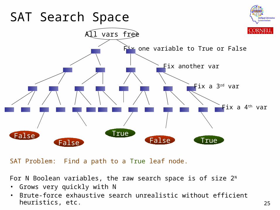
SAT Search Space
SAT Problem: Find a path to a True leaf node.
For N Boolean variables, the raw search space is of size 2N
• Grows very quickly with N• Brute-force exhaustive search unrealistic without efficient heuristics, etc.
All vars free
Fix one variable to True or False
Fix another var
Fix a 3rd var
TrueTrueFalse False
False
Fix a 4th var
27
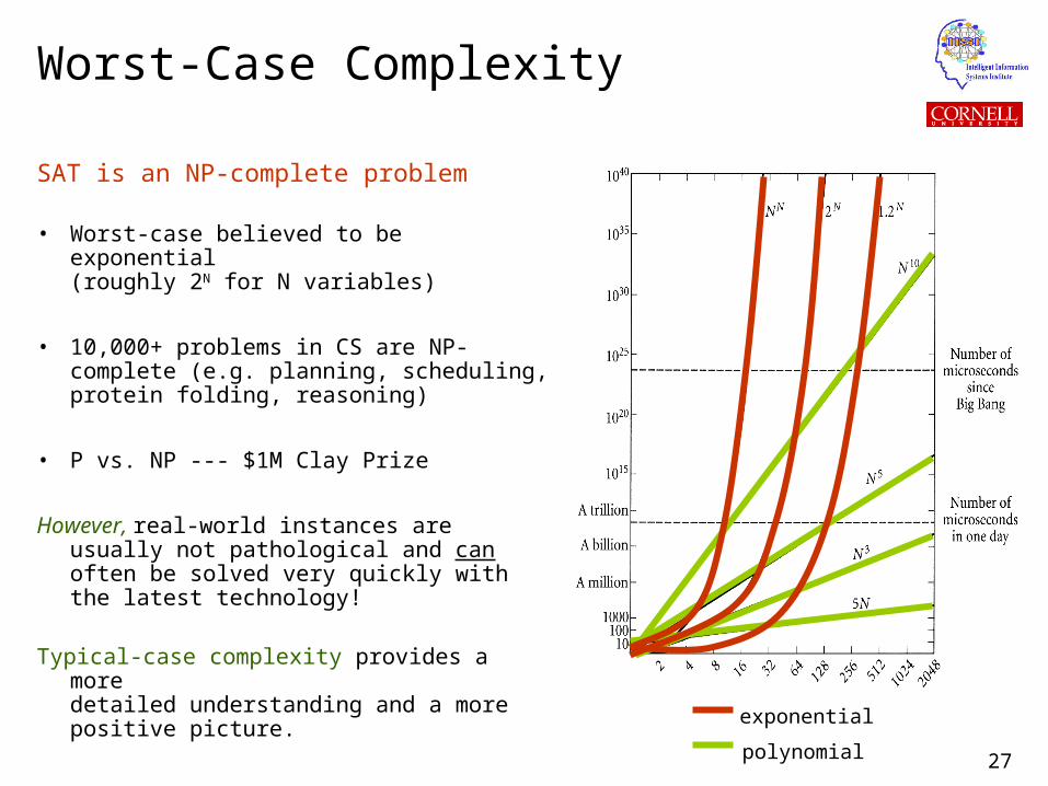
Worst-Case Complexity
SAT is an NP-complete problem
• Worst-case believed to be exponential(roughly 2N for N variables)
• 10,000+ problems in CS are NP-complete (e.g. planning, scheduling, protein folding, reasoning)
• P vs. NP --- $1M Clay Prize
However, real-world instances are usually not pathological and can often be solved very quickly with the latest technology!
Typical-case complexity provides a moredetailed understanding and a more positive picture.
exponential
polynomial
28
Tutorial Roadmap
Automated reasoning The complexity challenge State of the art in Boolean reasoning
2. SAT-based reasoning Boolean logic Search space, worst-case complexity Hardness profiles, scaling in practice– Modeling problems as SAT
• Example domain: planning
3. QBF reasoning (extends SAT)– A new range of applications– Two motivating examples
• network planning, logistics planning
– Quantified Boolean logic– Modeling problems as QBF– Search space, worst-case complexity– Scaling in practice
4. High-Performance QBF reasoning– Key research advances– The technology behind QBF– A. New modeling techniques– B. Learning while reasoning– C. Structure discovery– Experimental Results
5. Summary
29
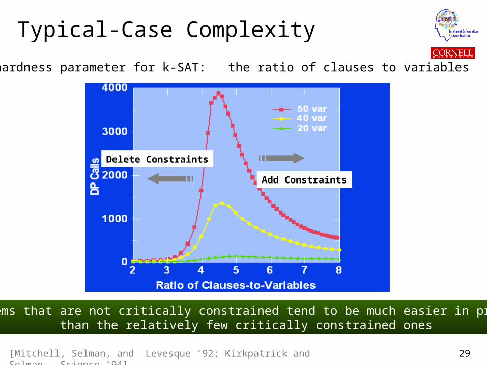
Typical-Case Complexity
A key hardness parameter for k-SAT: the ratio of clauses to variables
Add Constraints
Delete Constraints
Problems that are not critically constrained tend to be much easier in practicethan the relatively few critically constrained ones
[Mitchell, Selman, and Levesque ’92; Kirkpatrick and Selman – Science ’94]
30
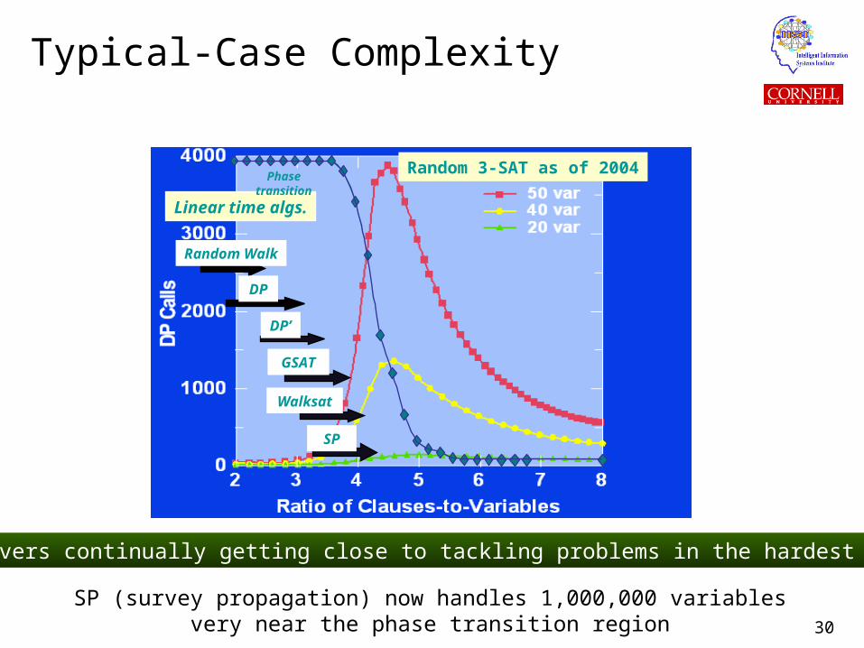
Typical-Case Complexity
Random 3-SAT as of 2004
Random Walk
DP
DP’
Walksat
SP
Linear time algs.
GSAT
Phase transition
SAT solvers continually getting close to tackling problems in the hardest region!
SP (survey propagation) now handles 1,000,000 variablesvery near the phase transition region
31
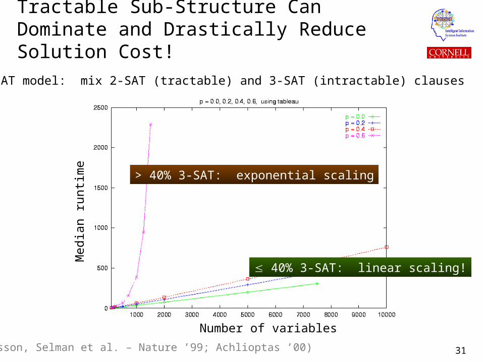
Tractable Sub-Structure Can Dominate and Drastically Reduce Solution Cost!
2+p-SAT model: mix 2-SAT (tractable) and 3-SAT (intractable) clauses
> 40% 3-SAT: exponential scaling
40% 3-SAT: linear scaling!
(Monasson, Selman et al. – Nature ’99; Achlioptas ’00)
Number of variables
Med
ian
runt
ime
32
Tutorial Roadmap
Automated reasoning The complexity challenge State of the art in Boolean reasoning
2. SAT-based reasoning Boolean logic Search space, worst-case complexity Hardness profiles, scaling in practice Modeling problems as SAT
• Example domain: planning
3. QBF reasoning (extends SAT)– A new range of applications– Two motivating examples
• network planning, logistics planning
– Quantified Boolean logic– Modeling problems as QBF– Search space, worst-case complexity– Scaling in practice
4. High-Performance QBF reasoning– Key research advances– The technology behind QBF– A. New modeling techniques– B. Learning while reasoning– C. Structure discovery– Experimental Results
5. Summary
33
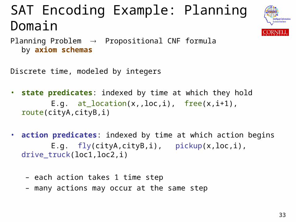
SAT Encoding Example: Planning Domain
Planning Problem Propositional CNF formulaby axiom schemas
Discrete time, modeled by integers
• state predicates: indexed by time at which they hold
E.g. at_location(x,,loc,i), free(x,i+1), route(cityA,cityB,i)
• action predicates: indexed by time at which action begins
E.g. fly(cityA,cityB,i), pickup(x,loc,i), drive_truck(loc1,loc2,i)
– each action takes 1 time step
– many actions may occur at the same step
34
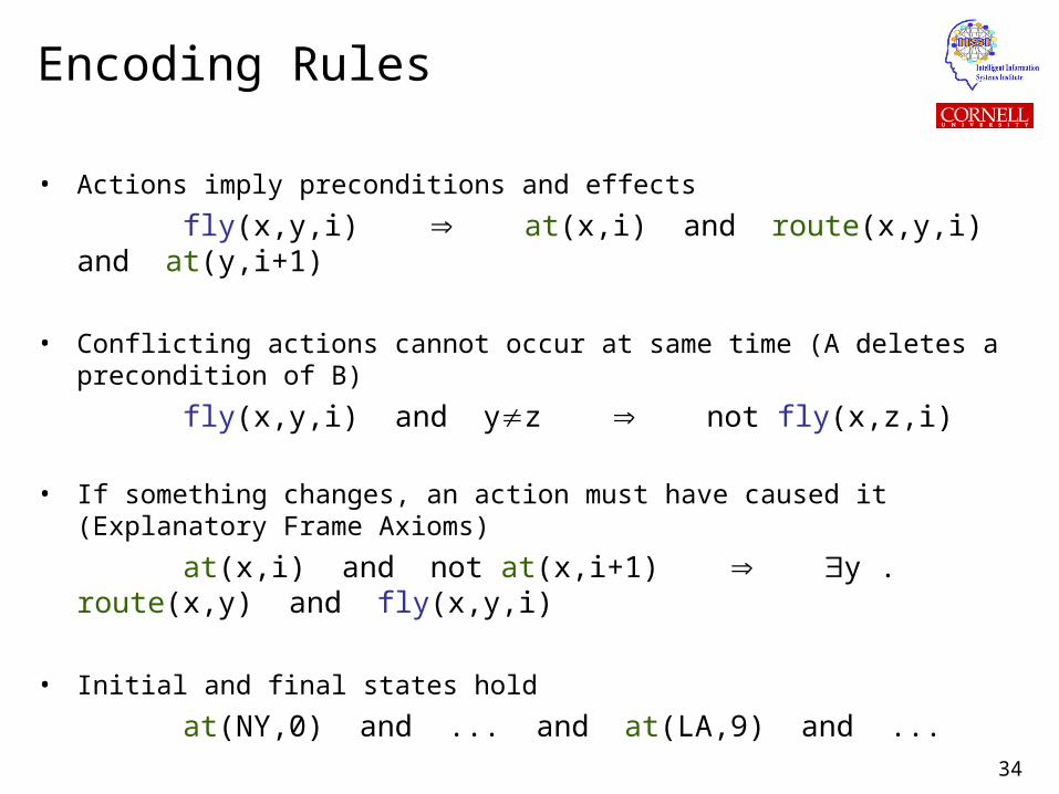
Encoding Rules
• Actions imply preconditions and effects
fly(x,y,i) at(x,i) and route(x,y,i) and at(y,i+1)
• Conflicting actions cannot occur at same time (A deletes a precondition of B)
fly(x,y,i) and yz not fly(x,z,i)
• If something changes, an action must have caused it(Explanatory Frame Axioms)
at(x,i) and not at(x,i+1) y . route(x,y) and fly(x,y,i)
• Initial and final states hold
at(NY,0) and ... and at(LA,9) and ...
36
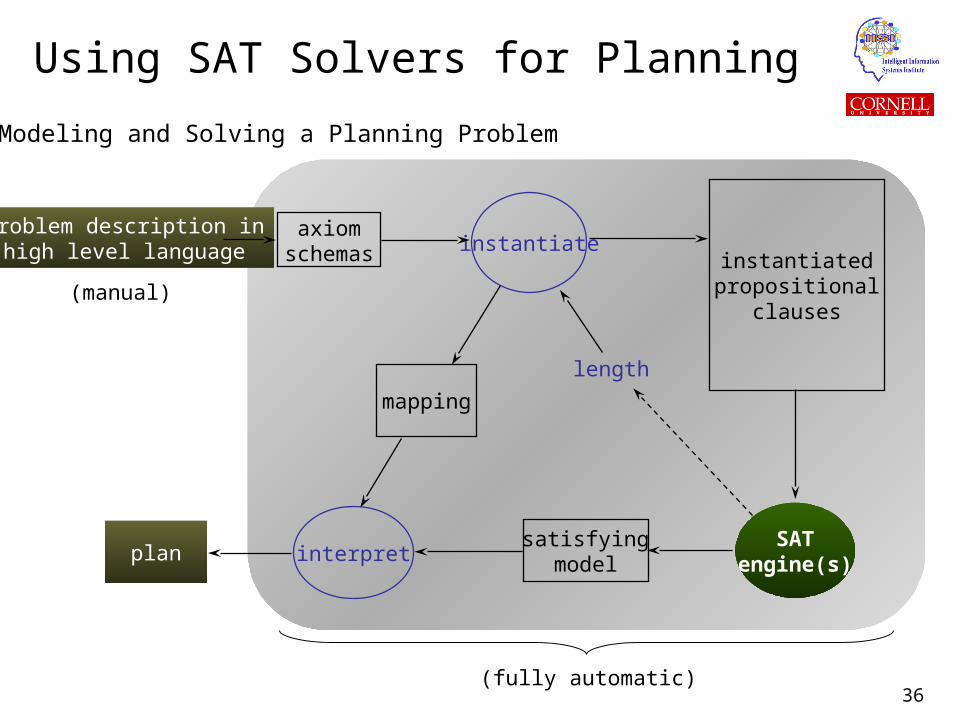
Using SAT Solvers for Planning
axiomschemas instantiated
propositionalclauses
satisfyingmodelplan
mapping
length
Problem description inhigh level language
SATengine(s)
instantiate
interpret
Modeling and Solving a Planning Problem
(fully automatic)
(manual)
39
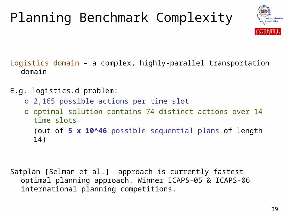
Planning Benchmark Complexity
Logistics domain – a complex, highly-parallel transportation domain
E.g. logistics.d problem:
o 2,165 possible actions per time slot
o optimal solution contains 74 distinct actions over 14 time slots
(out of 5 x 10^46 possible sequential plans of length 14)
Satplan [Selman et al.] approach is currently fastest optimal planning approach. Winner ICAPS-05 & ICAPS-06 international planning competitions.
40
Tutorial Roadmap
Automated reasoning The complexity challenge State of the art in Boolean reasoning
SAT-based reasoning Boolean logic Search space, worst-case complexity Hardness profiles, scaling in practice Modeling problems as SAT
Example domain: planning
3. QBF reasoning (extends SAT) A new range of applications– Two motivating examples
• network planning, logistics planning
– Quantified Boolean logic– Modeling problems as QBF– Search space, worst-case complexity– Scaling in practice
4. High-Performance QBF reasoning– Key research advances– The technology behind QBF– A. New modeling techniques– B. Learning while reasoning– C. Structure discovery– Experimental Results
5. Summary
41
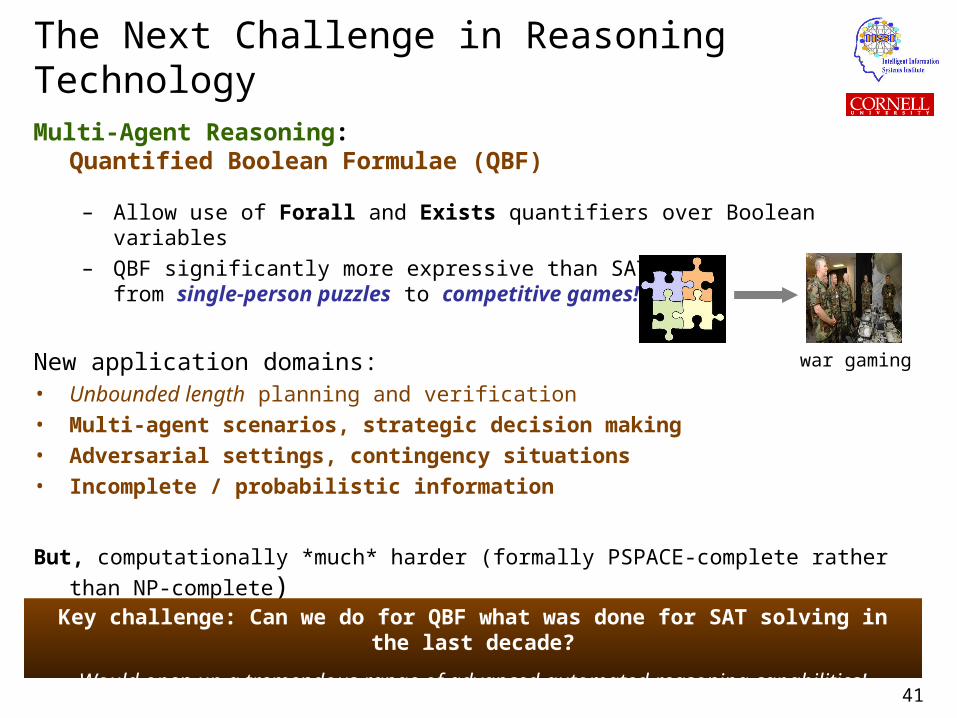
The Next Challenge in Reasoning Technology
Multi-Agent Reasoning:Quantified Boolean Formulae (QBF)
– Allow use of Forall and Exists quantifiers over Boolean variables– QBF significantly more expressive than SAT:
from single-person puzzles to competitive games!
New application domains:• Unbounded length planning and verification• Multi-agent scenarios, strategic decision making• Adversarial settings, contingency situations• Incomplete / probabilistic information
But, computationally *much* harder (formally PSPACE-complete rather than NP-complete)
Key challenge: Can we do for QBF what was done for SAT solving in the last decade?
Would open up a tremendous range of advanced automated reasoning capabilities!
war gaming
42
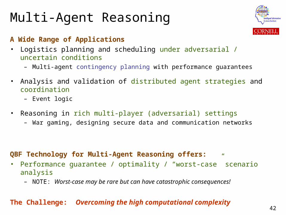
Multi-Agent Reasoning
A Wide Range of Applications
• Logistics planning and scheduling under adversarial / uncertain conditions– Multi-agent contingency planning with performance guarantees
• Analysis and validation of distributed agent strategies and coordination – Event logic
• Reasoning in rich multi-player (adversarial) settings– War gaming, designing secure data and communication networks
QBF Technology for Multi-Agent Reasoning offers:
• Performance guarantee / optimality / “worst-case” scenario analysis– NOTE: Worst-case may be rare but can have catastrophic consequences!
The Challenge: Overcoming the high computational complexity
43
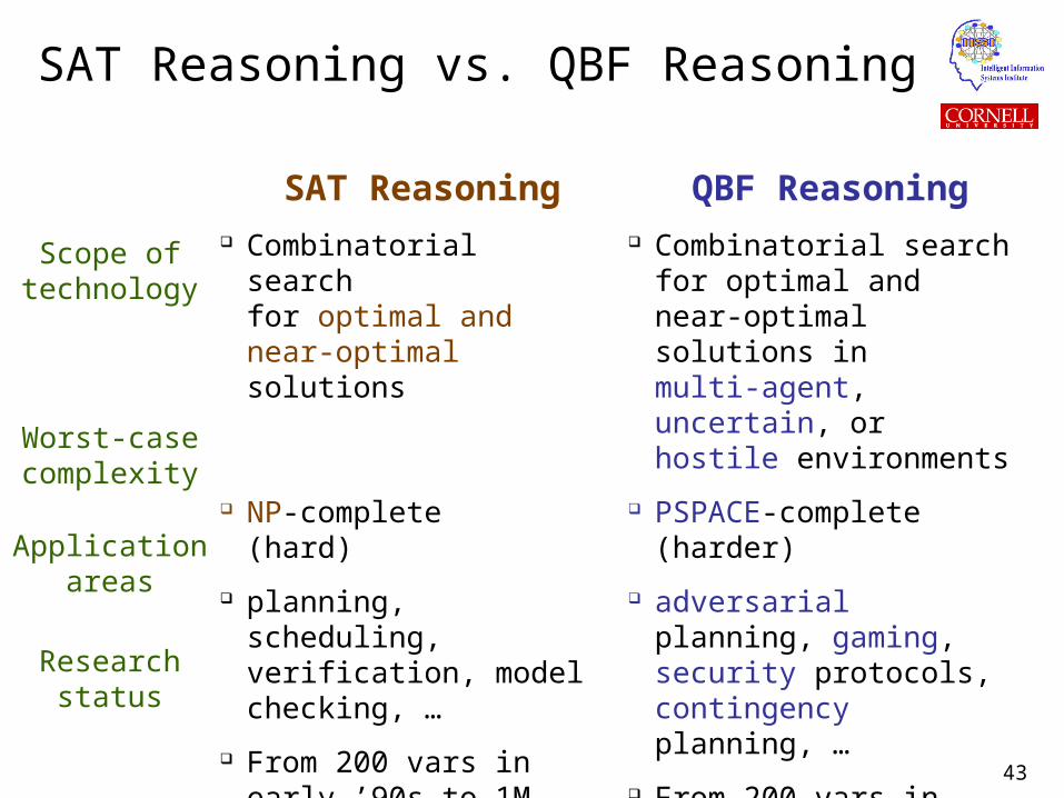
SAT Reasoning vs. QBF Reasoning
SAT Reasoning Combinatorial search
for optimal and near-optimal solutions
NP-complete(hard)
planning, scheduling, verification, model checking, …
From 200 vars in early ’90s to 1M vars. Now a commercially viable technology.
QBF Reasoning Combinatorial search
for optimal and near-optimal solutions in multi-agent, uncertain, orhostile environments
PSPACE-complete(harder)
adversarial planning, gaming, security protocols, contingency planning, …
From 200 vars in late 90’s to 100K vars currently. Still rapidly moving.
Scope oftechnology
Worst-casecomplexity
Applicationareas
Researchstatus
44
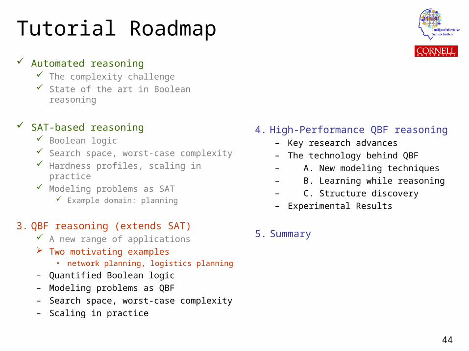
Tutorial Roadmap
Automated reasoning The complexity challenge State of the art in Boolean reasoning
SAT-based reasoning Boolean logic Search space, worst-case complexity Hardness profiles, scaling in practice Modeling problems as SAT
Example domain: planning
3. QBF reasoning (extends SAT) A new range of applications Two motivating examples
• network planning, logistics planning
– Quantified Boolean logic– Modeling problems as QBF– Search space, worst-case complexity– Scaling in practice
4. High-Performance QBF reasoning– Key research advances– The technology behind QBF– A. New modeling techniques– B. Learning while reasoning– C. Structure discovery– Experimental Results
5. Summary
45
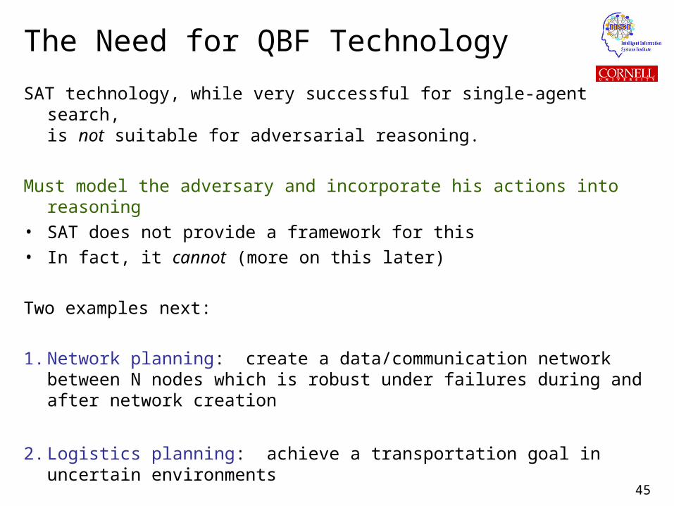
The Need for QBF Technology
SAT technology, while very successful for single-agent search, is not suitable for adversarial reasoning.
Must model the adversary and incorporate his actions into reasoning• SAT does not provide a framework for this• In fact, it cannot (more on this later)
Two examples next:
1. Network planning: create a data/communication network between N nodes which is robust under failures during and after network creation
2. Logistics planning: achieve a transportation goal in uncertain environments
46
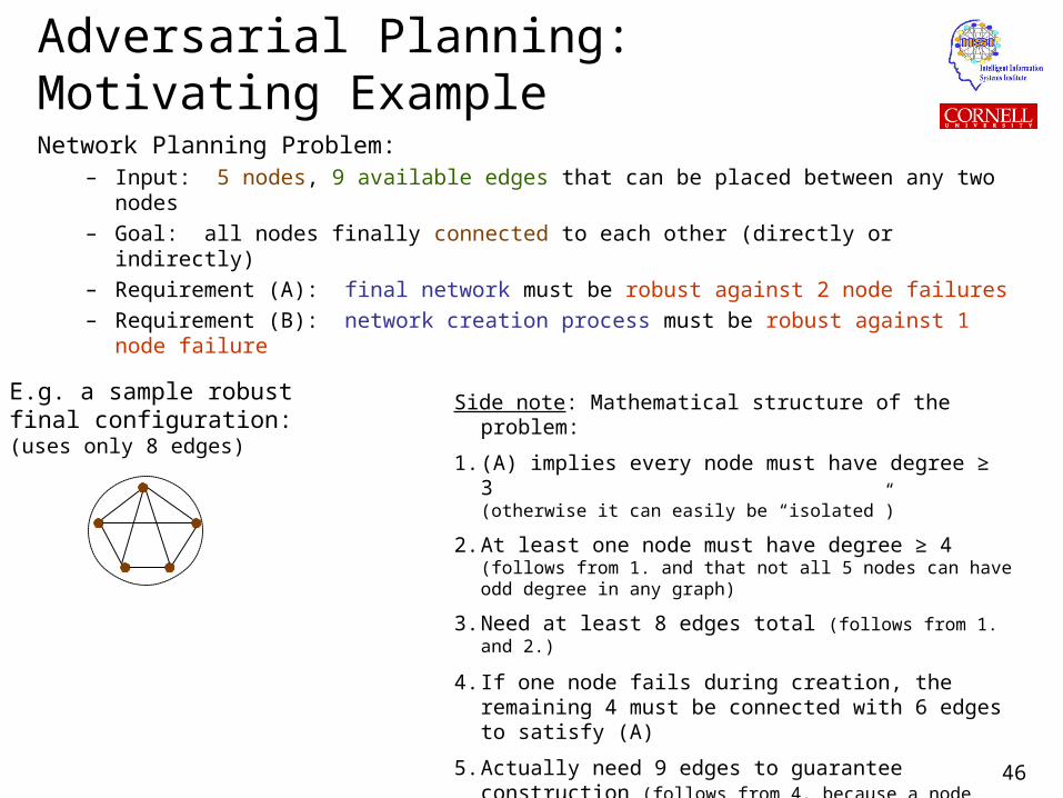
Adversarial Planning: Motivating Example
Network Planning Problem:– Input: 5 nodes, 9 available edges that can be placed between any two nodes– Goal: all nodes finally connected to each other (directly or indirectly)– Requirement (A): final network must be robust against 2 node failures– Requirement (B): network creation process must be robust against 1 node failure
E.g. a sample robust final configuration:(uses only 8 edges)
Side note: Mathematical structure of the problem:
1. (A) implies every node must have degree ≥ 3(otherwise it can easily be “isolated”)
2. At least one node must have degree ≥ 4(follows from 1. and that not all 5 nodes can have odd degree in any graph)
3. Need at least 8 edges total (follows from 1. and 2.)
4. If one node fails during creation, the remaining 4 must be connected with 6 edges to satisfy (A)
5. Actually need 9 edges to guarantee construction (follows from 4. because a node may fail as soon as its degree becomes 3)
47
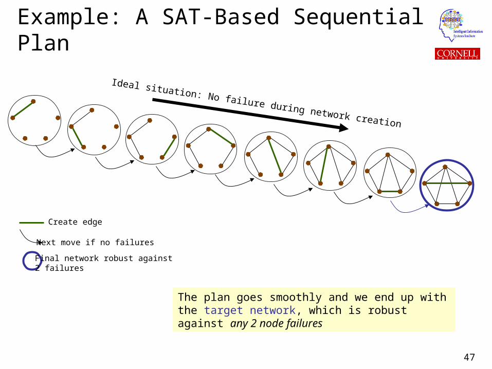
Example: A SAT-Based Sequential Plan
Ideal situation: No failure during network creation
The plan goes smoothly and we end up with the target network, which is robust against any 2 node failures
Create edge
Next move if no failures
Final network robust against2 failures
48
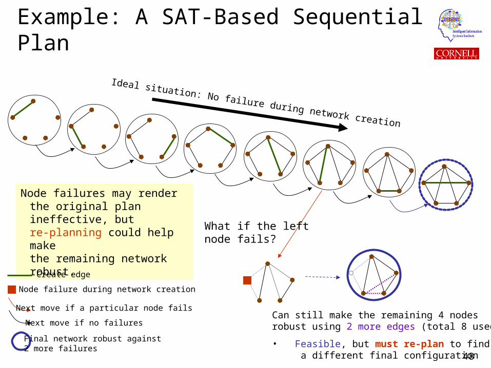
Example: A SAT-Based Sequential Plan
What if the leftnode fails?
Can still make the remaining 4 nodesrobust using 2 more edges (total 8 used)
• Feasible, but must re-plan to find a different final configuration
Ideal situation: No failure during network creation
Node failures may render the original plan ineffective, but re-planning could help makethe remaining network robust.
Create edge
Node failure during network creation
Next move if a particular node fails
Next move if no failures
Final network robust against2 more failures
49
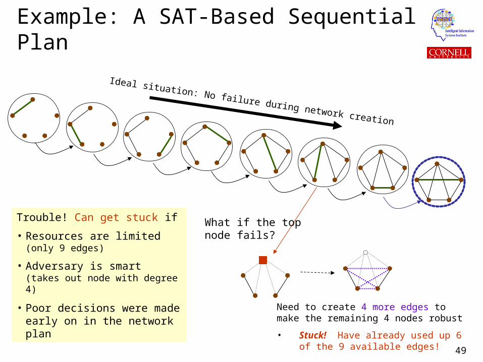
Example: A SAT-Based Sequential Plan
What if the topnode fails?
Need to create 4 more edges tomake the remaining 4 nodes robust
• Stuck! Have already used up 6 of the 9 available edges!
Ideal situation: No failure during network creation
Trouble! Can get stuck if
• Resources are limited(only 9 edges)
• Adversary is smart(takes out node with degree 4)
• Poor decisions were made early on in the network plan
50
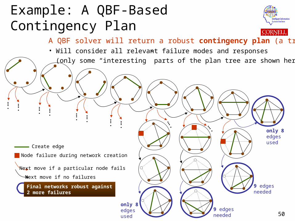
Example: A QBF-Based Contingency Plan
A QBF solver will return a robust contingency plan (a tree)• Will consider all relevant failure modes and responses
(only some “interesting” parts of the plan tree are shown here)
9 edgesneeded
only 8edgesused
9 edgesneeded
only 8edgesused
Create edge
Node failure during network creation
Next move if a particular node fails
Next move if no failures…
.
….
….
Final networks robust against2 more failures
….
….
….
….
….
….
….
51
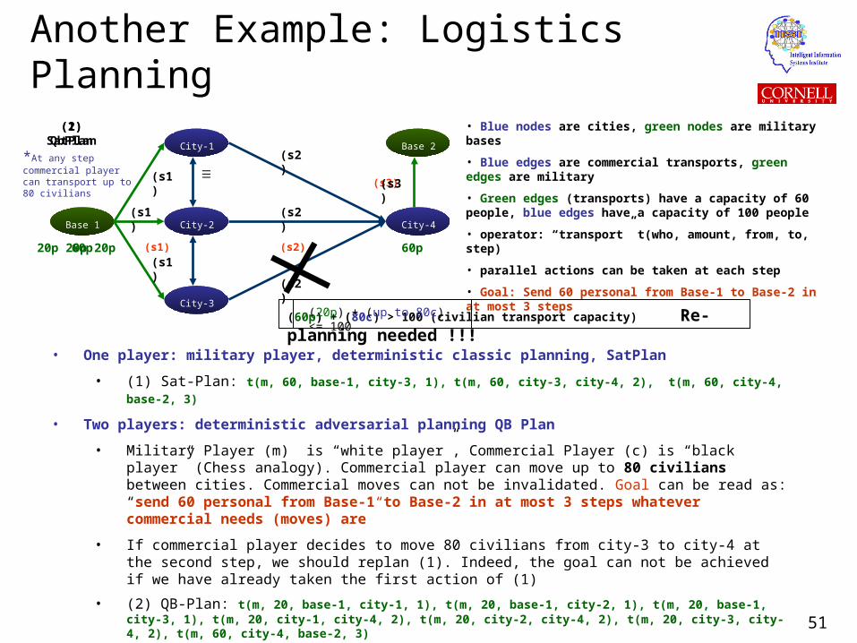
Another Example: Logistics Planning
Base 1
City-1
City-2 City-4
Base 2
City-3
• Blue nodes are cities, green nodes are military bases
• Blue edges are commercial transports, green edges are military
• Green edges (transports) have a capacity of 60 people, blue edges have a capacity of 100 people
• operator: “transport” t(who, amount, from, to, step)
• parallel actions can be taken at each step
• Goal: Send 60 personal from Base-1 to Base-2 in at most 3 steps
60p
• One player: military player, deterministic classic planning, SatPlan
• (1) Sat-Plan: t(m, 60, base-1, city-3, 1), t(m, 60, city-3, city-4, 2), t(m, 60, city-4, base-2, 3)
• Two players: deterministic adversarial planning QB Plan
• Military Player (m) is “white player”, Commercial Player (c) is “black player” (Chess analogy). Commercial player can move up to 80 civilians between cities. Commercial moves can not be invalidated. Goal can be read as: “send 60 personal from Base-1 to Base-2 in at most 3 steps whatever commercial needs (moves) are”
• If commercial player decides to move 80 civilians from city-3 to city-4 at the second step, we should replan (1). Indeed, the goal can not be achieved if we have already taken the first action of (1)
• (2) QB-Plan: t(m, 20, base-1, city-1, 1), t(m, 20, base-1, city-2, 1), t(m, 20, base-1, city-3, 1), t(m, 20, city-1, city-4, 2), t(m, 20, city-2, city-4, 2), t(m, 20, city-3, city-4, 2), t(m, 60, city-4, base-2, 3)
(1) SatPlan
(s1) (s2)
(s3)
*At any step commercial player can transport up to 80 civilians
(60p) + (80c) > 100 (civilian transport capacity) Re-planning needed !!!
(2) QbPlan
20p20p 20p
(s1)
(s1)
(s1)
(s2)
(s2)
(s2)
60p
(s3)
(20p) + (up to 80c) <= 100
52
Tutorial Roadmap
Automated reasoning The complexity challenge State of the art in Boolean reasoning
SAT-based reasoning Boolean logic Search space, worst-case complexity Hardness profiles, scaling in practice Modeling problems as SAT
Example domain: planning
3. QBF reasoning (extends SAT) A new range of applications Two motivating examples
network planning, logistics planning
Quantified Boolean logic– Modeling problems as QBF– Search space, worst-case complexity– Scaling in practice
4. High-Performance QBF reasoning– Key research advances– The technology behind QBF– A. New modeling techniques– B. Learning while reasoning– C. Structure discovery– Experimental Results
5. Summary
53
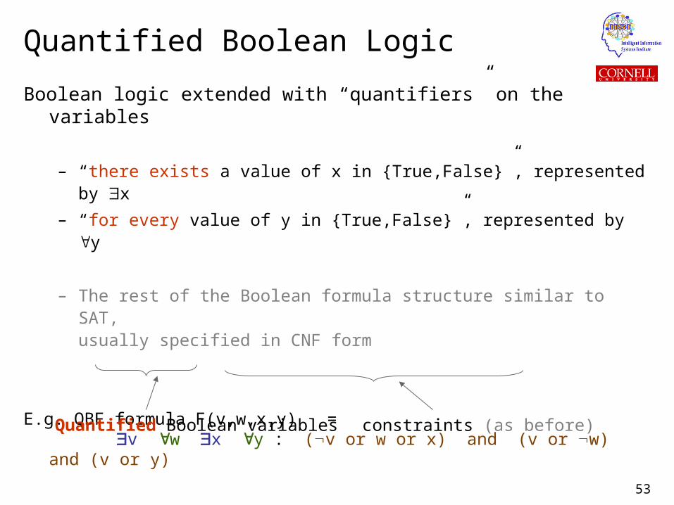
Boolean logic extended with “quantifiers” on the variables
– “there exists a value of x in {True,False}”, represented by x
– “for every value of y in {True,False}”, represented by y
– The rest of the Boolean formula structure similar to SAT,usually specified in CNF form
E.g. QBF formula F(v,w,x,y) = v w x y : (v or w or x) and (v or w) and (v or y)
Quantified Boolean Logic
Quantified Boolean variables constraints (as before)
54
Quantified Boolean Logic: Semantics
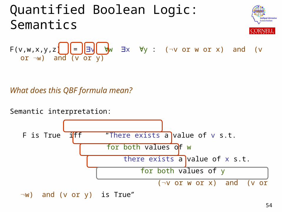
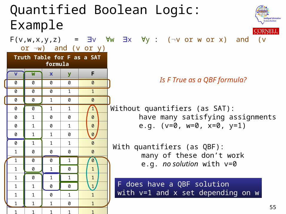
F(v,w,x,y,z) = v w x y : (v or w or x) and (v or w) and (v or y)
What does this QBF formula mean?
Semantic interpretation:
F is True iff “There exists a value of v s.t.
for both values of w
there exists a value of x s.t.
for both values of y
(v or w or x) and (v or w) and (v or y) is
True”
55
Quantified Boolean Logic: Example
F(v,w,x,y,z) = v w x y : (v or w or x) and (v or w) and (v or y)
Truth Table for F as a SAT formula
v w x y F
0 0 0 0 0
0 0 0 1 1
0 0 1 0 0
0 0 1 1 1
0 1 0 0 0
0 1 0 1 0
0 1 1 0 0
0 1 1 1 0
1 0 0 0 0
1 0 0 1 0
1 0 1 0 1
1 0 1 1 1
1 1 0 0 1
1 1 0 1 1
1 1 1 0 1
1 1 1 1 1
Is F True as a QBF formula?
Without quantifiers (as SAT):have many satisfying assignmentse.g. (v=0, w=0, x=0, y=1)
With quantifiers (as QBF):many of these don’t worke.g. no solution with v=0
F does have a QBF solutionwith v=1 and x set depending on w
56
Tutorial Roadmap
Automated reasoning The complexity challenge State of the art in Boolean reasoning
SAT-based reasoning Boolean logic Search space, worst-case complexity Hardness profiles, scaling in practice Modeling problems as SAT
Example domain: planning
3. QBF reasoning (extends SAT) A new range of applications Two motivating examples
network planning, logistics planning
Quantified Boolean logic Modeling problems as QBF– Search space, worst-case complexity– Scaling in practice
4. High-Performance QBF reasoning– Key research advances– The technology behind QBF– A. New modeling techniques– B. Learning while reasoning– C. Structure discovery– Experimental Results
5. Summary
57
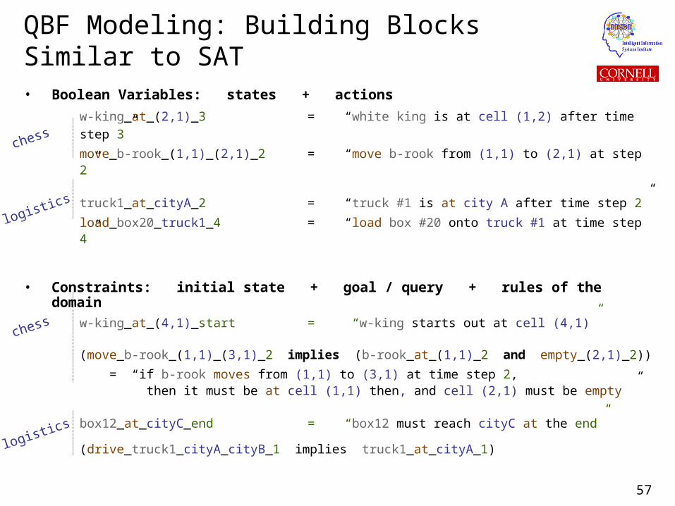
QBF Modeling: Building Blocks Similar to SAT
• Boolean Variables: states + actions
w-king_at_(2,1)_3 = “white king is at cell (1,2) after time step 3”
move_b-rook_(1,1)_(2,1)_2 = “move b-rook from (1,1) to (2,1) at step 2”
truck1_at_cityA_2 = “truck #1 is at city A after time step 2”
load_box20_truck1_4 = “load box #20 onto truck #1 at time step 4”
• Constraints: initial state + goal / query + rules of the domain
w-king_at_(4,1)_start = “w-king starts out at cell (4,1)”
(move_b-rook_(1,1)_(3,1)_2 implies (b-rook_at_(1,1)_2 and empty_(2,1)_2))
= “if b-rook moves from (1,1) to (3,1) at time step 2, then it must be at cell (1,1) then, and cell (2,1) must be empty ”
box12_at_cityC_end = “box12 must reach cityC at the end”
(drive_truck1_cityA_cityB_1 implies truck1_at_cityA_1)
chess
chess
logistics
logistics
58
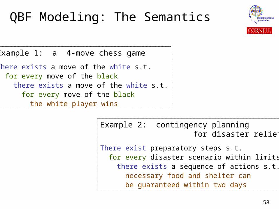
QBF Modeling: The Semantics
Example 1: a 4-move chess game
There exists a move of the white s.t. for every move of the black there exists a move of the white s.t. for every move of the black the white player wins
Example 2: contingency planning for disaster relief
There exist preparatory steps s.t. for every disaster scenario within limits there exists a sequence of actions s.t. necessary food and shelter can be guaranteed within two days
59
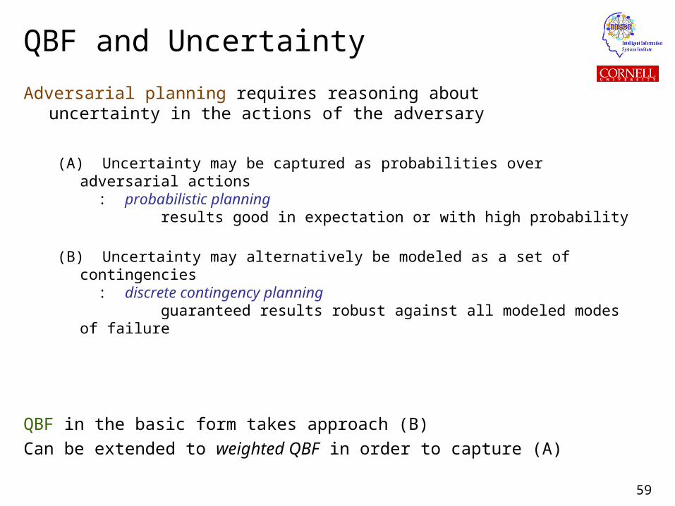
QBF and Uncertainty
Adversarial planning requires reasoning about uncertainty in the actions of the adversary
(A) Uncertainty may be captured as probabilities over adversarial actions : probabilistic planning results good in expectation or with high probability
(B) Uncertainty may alternatively be modeled as a set of contingencies : discrete contingency planning guaranteed results robust against all modeled modes of failure
QBF in the basic form takes approach (B)
Can be extended to weighted QBF in order to capture (A)
60
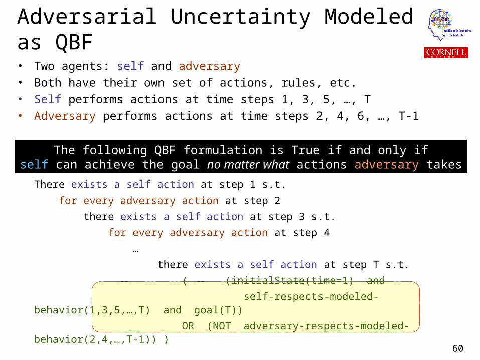
Adversarial Uncertainty Modeled as QBF
• Two agents: self and adversary
• Both have their own set of actions, rules, etc.
• Self performs actions at time steps 1, 3, 5, …, T
• Adversary performs actions at time steps 2, 4, 6, …, T-1
There exists a self action at step 1 s.t.
for every adversary action at step 2
there exists a self action at step 3 s.t.
for every adversary action at step 4
…
there exists a self action at step T s.t.
( (initialState(time=1) and
self-respects-modeled-behavior(1,3,5,…,T) and goal(T))
OR (NOT adversary-respects-modeled-behavior(2,4,…,T-1)) )
The following QBF formulation is True if and only ifself can achieve the goal no matter what actions adversary takes
61
Tutorial Roadmap
Automated reasoning The complexity challenge State of the art in Boolean reasoning
SAT-based reasoning Boolean logic Search space, worst-case complexity Hardness profiles, scaling in practice Modeling problems as SAT
Example domain: planning
3. QBF reasoning (extends SAT) A new range of applications Two motivating examples
network planning, logistics planning
Quantified Boolean logic Modeling problems as QBF Search space, worst-case complexity– Scaling in practice
4. High-Performance QBF reasoning– Key research advances– The technology behind QBF– A. New modeling techniques– B. Learning while reasoning– C. Structure discovery– Experimental Results
5. Summary
62
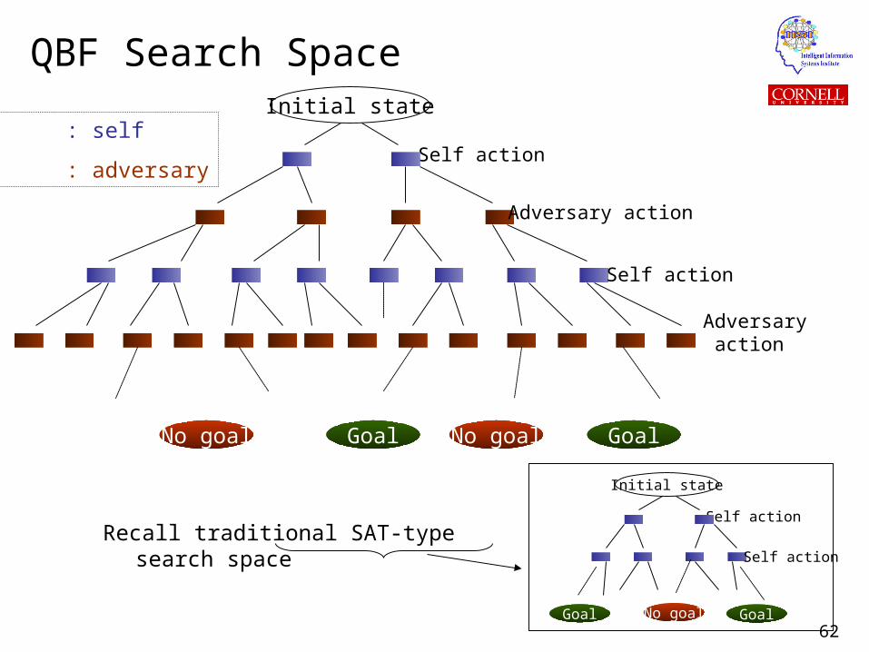
QBF Search Space
Recall traditional SAT-type search space
Adversary action
Self action
Adversary action
Initial state
Self action
Goal GoalNo goal No goal
Self action
Self action
Initial state
Goal GoalNo goal
: self
: adversary
63
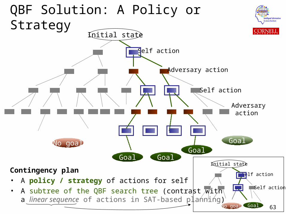
QBF Solution: A Policy or Strategy
Contingency plan
• A policy / strategy of actions for self
• A subtree of the QBF search tree (contrast with a linear sequence of actions in SAT-based planning)
Adversary action
Adversary action
Initial state
Self action
Self action
Self action
Self action
Initial state
GoalNo goal
Goal GoalGoal
No goal Goal
64
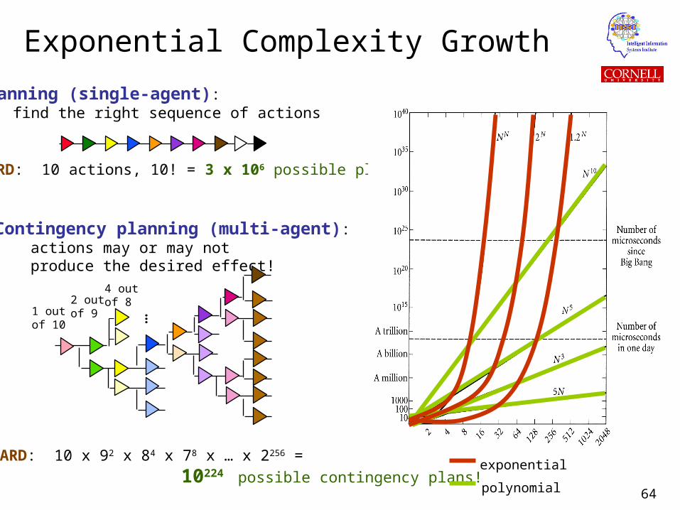
Exponential Complexity Growth
Planning (single-agent): find the right sequence of actions
HARD: 10 actions, 10! = 3 x 10⁶ possible plans
REALLY HARD: 10 x 92 x 84 x 78 x … x 2256 =
10224 possible contingency plans!
Contingency planning (multi-agent): actions may or may not produce the desired effect!
exponential
polynomial
…1 outof 10
2 outof 9
4 outof 8
65
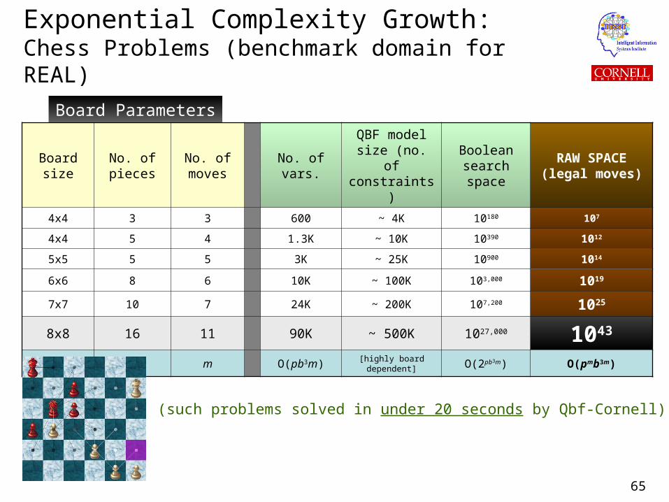
Exponential Complexity Growth:Chess Problems (benchmark domain for REAL)
Board size
No. of pieces
No. of moves
No. of vars.QBF model size (no. of constraints)
Boolean search space
RAW SPACE (legal moves)
4x4 3 3 600 ~ 4K 10180 107
4x4 5 4 1.3K ~ 10K 10390 1012
5x5 5 5 3K ~ 25K 10900 1014
6x6 8 6 10K ~ 100K 103,000 1019
7x7 10 7 24K ~ 200K 107,200 1025
8x8 16 11 90K ~ 500K 1027,000 1043
bxb p m O(pb3m) [highly board dependent] O(2pb3m) O(pmb3m)
(such problems solved in under 20 seconds by Qbf-Cornell)
Board Parameters
66
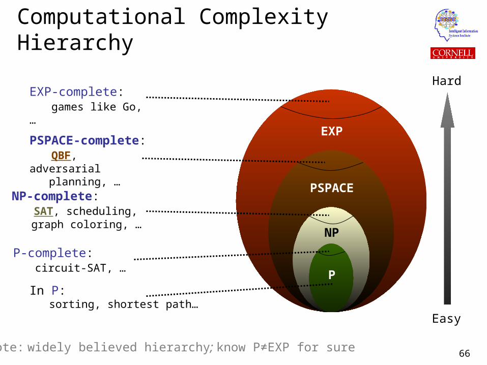
P
NP
PSPACE
EXP
NP-complete: SAT, scheduling, graph coloring, …
PSPACE-complete: QBF, adversarial planning, …
EXP-complete: games like Go, …
P-complete: circuit-SAT, …
Note: widely believed hierarchy; know P≠EXP for sure
In P: sorting, shortest path…
Computational Complexity Hierarchy
Easy
Hard
67
Tutorial Roadmap
Automated reasoning The complexity challenge State of the art in Boolean reasoning
SAT-based reasoning Boolean logic Search space, worst-case complexity Hardness profiles, scaling in practice Modeling problems as SAT
Example domain: planning
3. QBF reasoning (extends SAT) A new range of applications Two motivating examples
network planning, logistics planning
Quantified Boolean logic Modeling problems as QBF Search space, worst-case complexity Scaling in practice
4. High-Performance QBF reasoning– Key research advances– The technology behind QBF– A. New modeling techniques– B. Learning while reasoning– C. Structure discovery– Experimental Results
5. Summary
68
QBF Scaling Behavior in Practice
Although hard in the worst-case, QBF technology can scale well in practice.
• Real-world problems often have built-in structure and contain hidden tractable sub-problems that make QBF solvers much faster in practice.
(Note: This has helped make SAT-based single-agent reasoning scale to large problems with 1,000,000+ variables. We are pushing QBF toward this goal.)
• Qbf-Cornell and Qbf-CornellD can automatically exploit many hidden tractable sub-structures and regularities in the problem (scaling plots on the next few slides)
On many chess instances, we observe– either low-polynomial (or even near-linear) scaling– or exponential scaling but with a much lower exponent than raw search
69
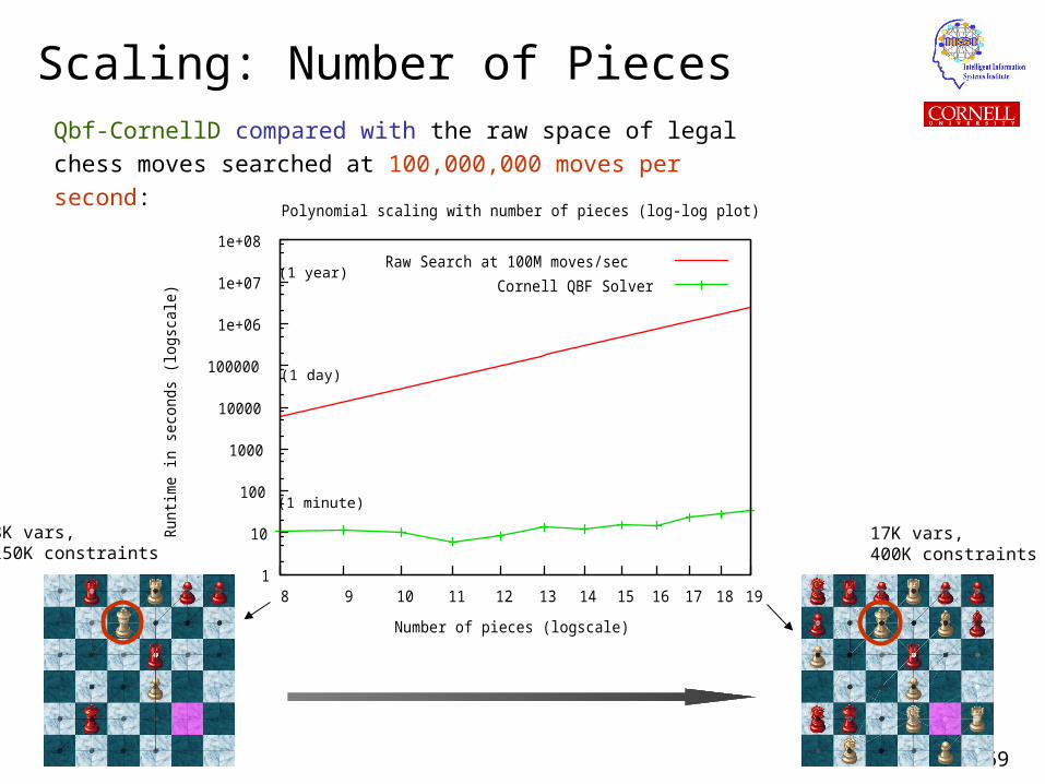
Scaling: Number of PiecesQbf-CornellD compared with the raw space of legal chess moves
searched at 100,000,000 moves per second:
8K vars,150K constraints
17K vars,400K constraints
1
10
100
1000
10000
100000
1e+06
1e+07
1e+08
19 18 17 16 15 14 13 12 11 10 9 8
Run
time
in s
econ
ds (l
ogsc
ale)
Number of pieces (logscale)
Polynomial scaling with number of pieces (log-log plot)
Raw Search at 100M moves/secCornell QBF Solver
(1 day)
(1 year)
(1 minute)
70
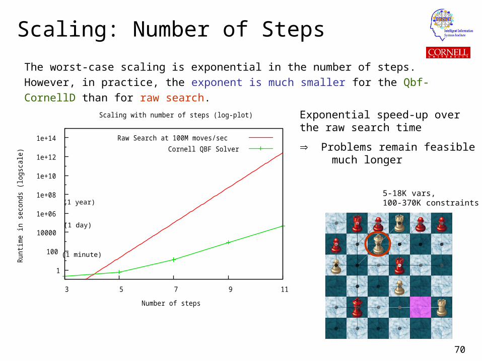
Scaling: Number of Steps
The worst-case scaling is exponential in the number of steps. However, in practice,
the exponent is much smaller for the Qbf-CornellD than for raw search.
Exponential speed-up overthe raw search time
Problems remain feasible much longer
1
100
10000
1e+06
1e+08
1e+10
1e+12
1e+14
3 5 7 9 11
Run
time
in s
econ
ds (l
ogsc
ale)
Number of steps
Scaling with number of steps (log-plot)
Raw Search at 100M moves/secCornell QBF Solver
(1 day)
(1 year)
(1 minute)
5-18K vars,100-370K constraints
71
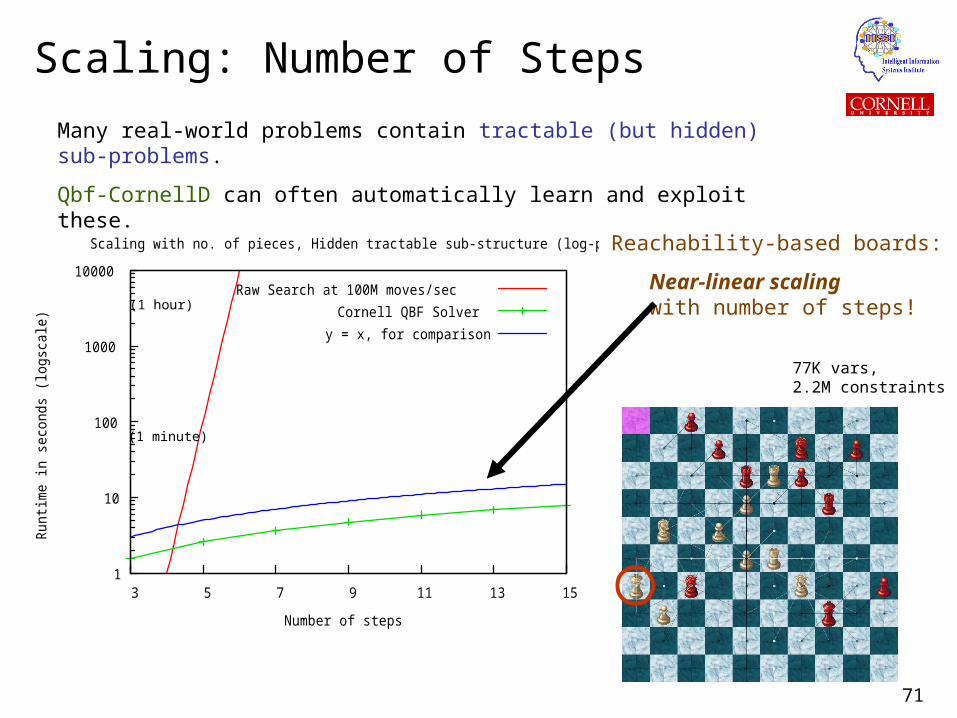
Scaling: Number of Steps
Many real-world problems contain tractable (but hidden) sub-problems.
Qbf-CornellD can often automatically learn and exploit these.
Reachability-based boards:
Near-linear scaling with number of steps!
1
10
100
1000
10000
3 5 7 9 11 13 15
Run
time
in s
econ
ds (l
ogsc
ale)
Number of steps
Scaling with no. of pieces, Hidden tractable sub-structure (log-plot)
Raw Search at 100M moves/secCornell QBF Solver
y = x, for comparison
(1 hour)
(1 minute)
77K vars,2.2M constraints
72
Tutorial Roadmap
Automated reasoning The complexity challenge State of the art in Boolean reasoning
SAT-based reasoning Boolean logic Search space, worst-case complexity Hardness profiles, scaling in practice Modeling problems as SAT
Example domain: planning
QBF reasoning (extends SAT) A new range of applications Two motivating examples
network planning, logistics planning
Quantified Boolean logic Modeling problems as QBF Search space, worst-case complexity Scaling in practice
4. High-Performance QBF reasoning Key research advances– The technology behind QBF– A. New modeling techniques– B. Learning while reasoning– C. Structure discovery– Experimental Results
5. Summary
73
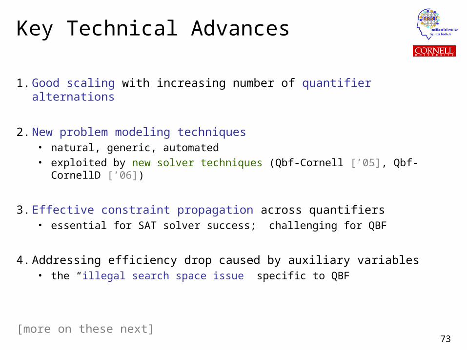
Key Technical Advances
1. Good scaling with increasing number of quantifier alternations
2. New problem modeling techniques• natural, generic, automated
• exploited by new solver techniques (Qbf-Cornell [’05], Qbf-CornellD [’06])
3. Effective constraint propagation across quantifiers• essential for SAT solver success; challenging for QBF
4. Addressing efficiency drop caused by auxiliary variables• the “illegal search space issue” specific to QBF
[more on these next]
74
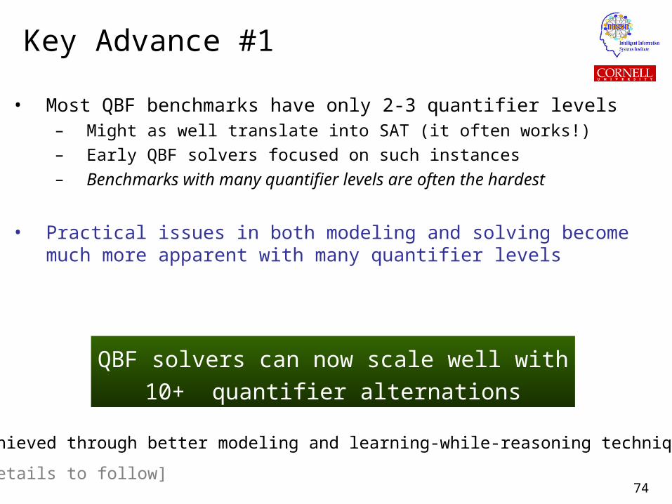
Key Advance #1
• Most QBF benchmarks have only 2-3 quantifier levels– Might as well translate into SAT (it often works!)
– Early QBF solvers focused on such instances
– Benchmarks with many quantifier levels are often the hardest
• Practical issues in both modeling and solving become much more apparent with many quantifier levels
QBF solvers can now scale well with
10+ quantifier alternations
Achieved through better modeling and learning-while-reasoning techniques.
[details to follow]
75
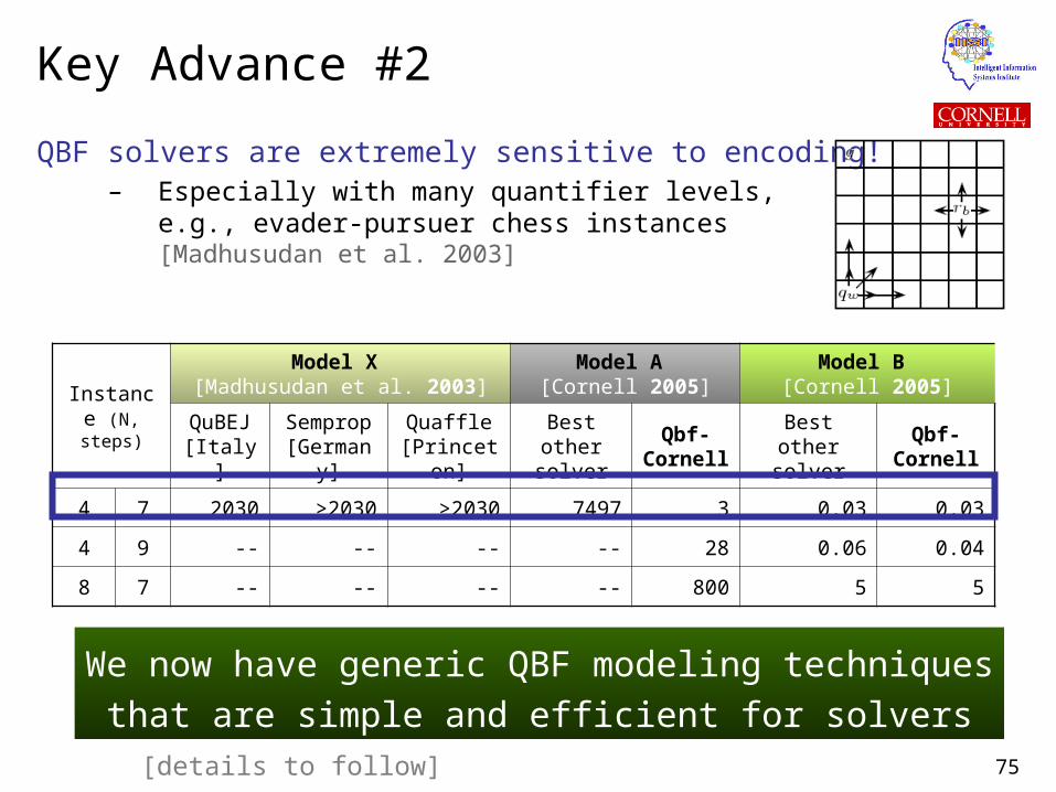
Key Advance #2
QBF solvers are extremely sensitive to encoding!– Especially with many quantifier levels,
e.g., evader-pursuer chess instances [Madhusudan et al. 2003]
Instance (N, steps)
Model X [Madhusudan et al. 2003]
Model A [Cornell 2005]
Model B [Cornell 2005]
QuBEJ [Italy]
Semprop [Germany]
Quaffle [Princeton]
Best other solver
Qbf-Cornell
Best other solver
Qbf-Cornell
4 7 2030 >2030 >2030 7497 3 0.03 0.03
4 9 -- -- -- -- 28 0.06 0.04
8 7 -- -- -- -- 800 5 5
We now have generic QBF modeling techniques
that are simple and efficient for solvers[details to follow]
76
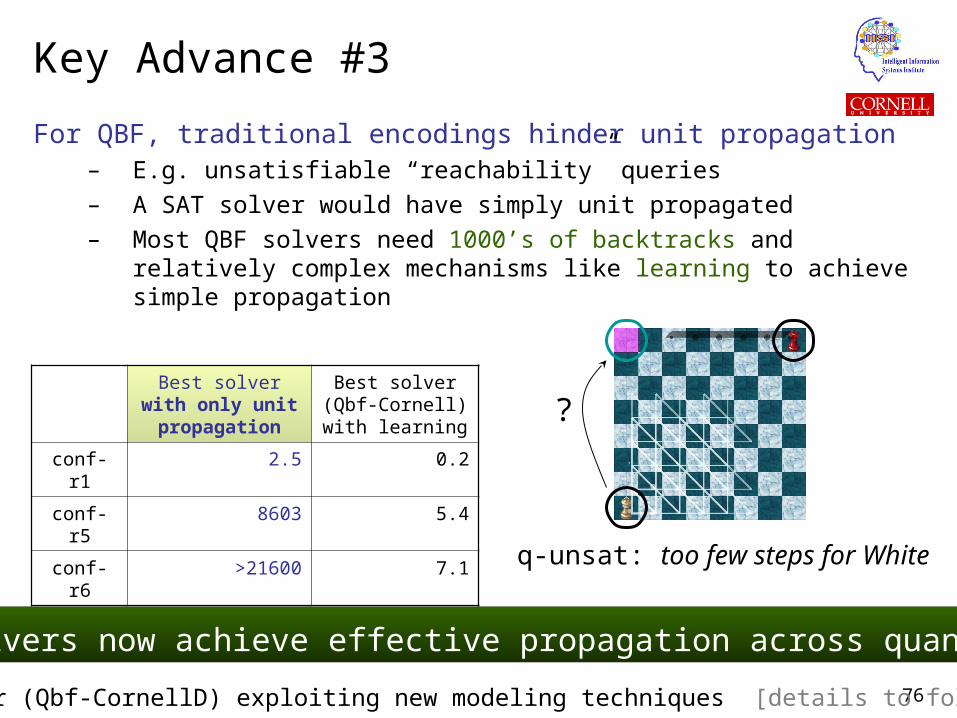
Key Advance #3
For QBF, traditional encodings hinder unit propagation– E.g. unsatisfiable “reachability” queries
– A SAT solver would have simply unit propagated
– Most QBF solvers need 1000’s of backtracks and relatively complex mechanisms like learning to achieve simple propagation
Best solverwith only unit propagation
Best solver(Qbf-Cornell)with learning
conf-r1 2.5 0.2
conf-r5 8603 5.4
conf-r6 >21600 7.1
q-unsat: too few steps for White
?
QBF solvers now achieve effective propagation across quantifiers
New solver (Qbf-CornellD) exploiting new modeling techniques [details to follow]
77
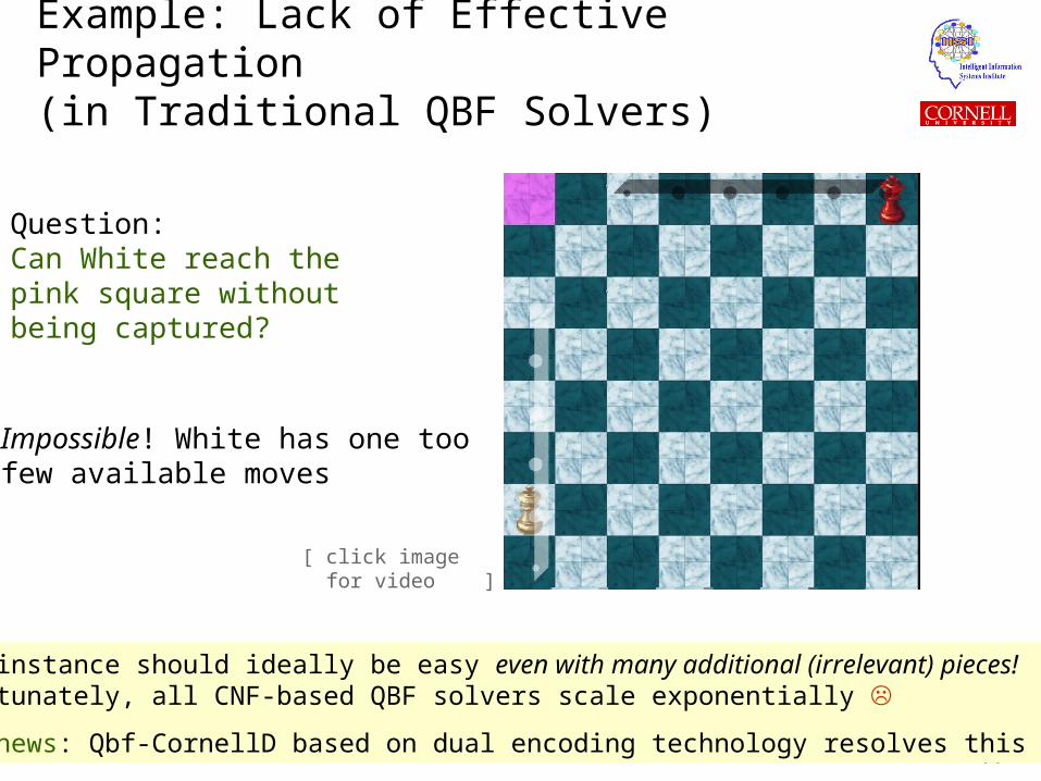
Example: Lack of Effective Propagation(in Traditional QBF Solvers)
Impossible! White has one toofew available moves
Question:Can White reach thepink square withoutbeing captured?
This instance should ideally be easy even with many additional (irrelevant) pieces!Unfortunately, all CNF-based QBF solvers scale exponentially
Good news: Qbf-CornellD based on dual encoding technology resolves this issue!
[ click image for video ]
78
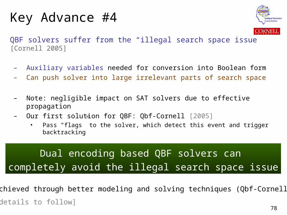
Key Advance #4
QBF solvers suffer from the “illegal search space issue”[Cornell 2005]
– Auxiliary variables needed for conversion into Boolean form
– Can push solver into large irrelevant parts of search space
– Note: negligible impact on SAT solvers due to effective propagation
– Our first solution for QBF: Qbf-Cornell [2005]• Pass “flags” to the solver, which detect this event and trigger backtracking
Dual encoding based QBF solvers can
completely avoid the illegal search space issue
Achieved through better modeling and solving techniques (Qbf-CornellD).
[details to follow]
79
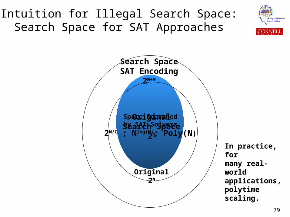
OriginalSearch Space
2N
Search SpaceSAT Encoding
2N+M
Space Searchedby SAT Solvers
2N/C ; Nlog(N); Poly(N)
Original2N
Intuition for Illegal Search Space:Search Space for SAT Approaches
In practice, formany real-worldapplications, polytime scaling.
80
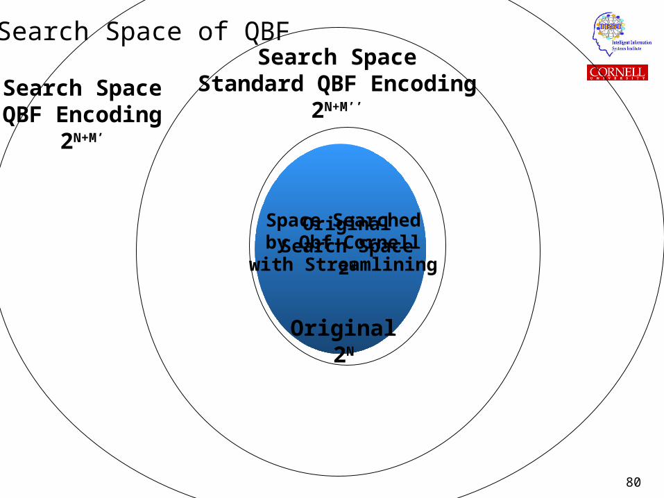
OriginalSearch Space
2N
Search SpaceQBF Encoding
2N+M’
Space Searchedby Qbf-Cornell
with Streamlining
Search Space of QBFSearch Space
Standard QBF Encoding2N+M’’
Original2N
81
Tutorial Roadmap
Automated reasoning The complexity challenge State of the art in Boolean reasoning
SAT-based reasoning Boolean logic Search space, worst-case complexity Hardness profiles, scaling in practice Modeling problems as SAT
Example domain: planning
QBF reasoning (extends SAT) A new range of applications Two motivating examples
network planning, logistics planning
Quantified Boolean logic Modeling problems as QBF Search space, worst-case complexity Scaling in practice
4. High-Performance QBF reasoning Key research advances The technology behind QBF– A. New modeling techniques– B. Learning while reasoning– C. Structure discovery– Experimental Results
5. Summary
82
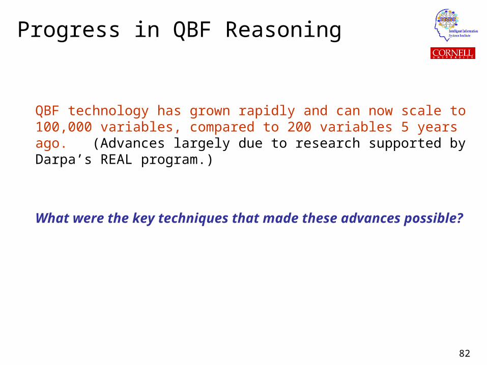
Progress in QBF Reasoning
QBF technology has grown rapidly and can now scale to 100,000 variables, compared to 200 variables 5 years ago. (Advances largely due to research supported by Darpa’s REAL program.)
What were the key techniques that made these advances possible?
83
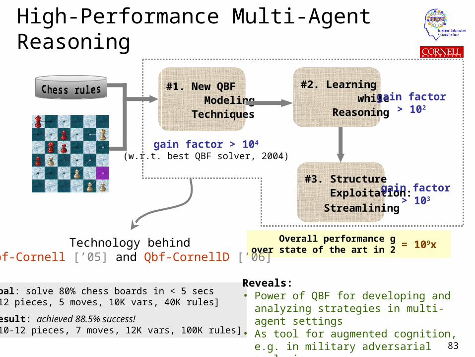
#1. New QBF Modeling Techniques
#2. Learning while Reasoning
#3. Structure Exploitation:
Streamlining
gain factor > 104
(w.r.t. best QBF solver, 2004)
gain factor> 102
gain factor> 103
Overall performance gainover state of the art in 2004 = 109x
Goal: solve 80% chess boards in < 5 secs [12 pieces, 5 moves, 10K vars, 40K rules]
Result: achieved 88.5% success![10-12 pieces, 7 moves, 12K vars, 100K rules]
Reveals:• Power of QBF for developing and analyzing
strategies in multi-agent settings• As tool for augmented cognition, e.g. in
military adversarial analysis
High-Performance Multi-Agent Reasoning
Technology behindQbf-Cornell [’05] and Qbf-CornellD [’06]
84
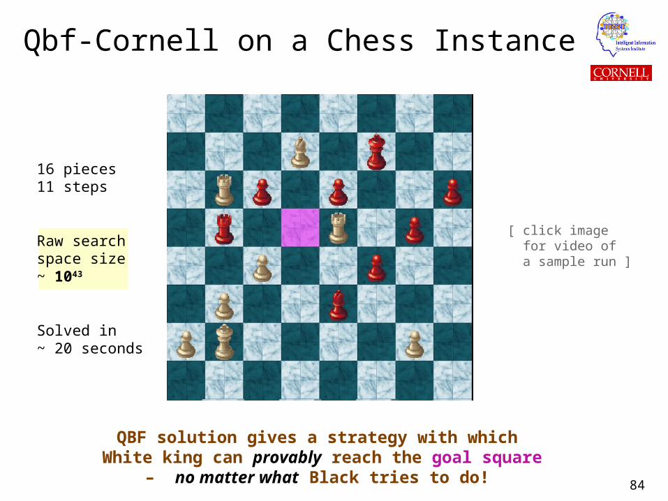
Qbf-Cornell on a Chess Instance
16 pieces11 steps
Raw searchspace size~ 1043
Solved in~ 20 seconds
QBF solution gives a strategy with which White king can provably reach the goal square
– no matter what Black tries to do!
[ click image for video of a sample run ]
85
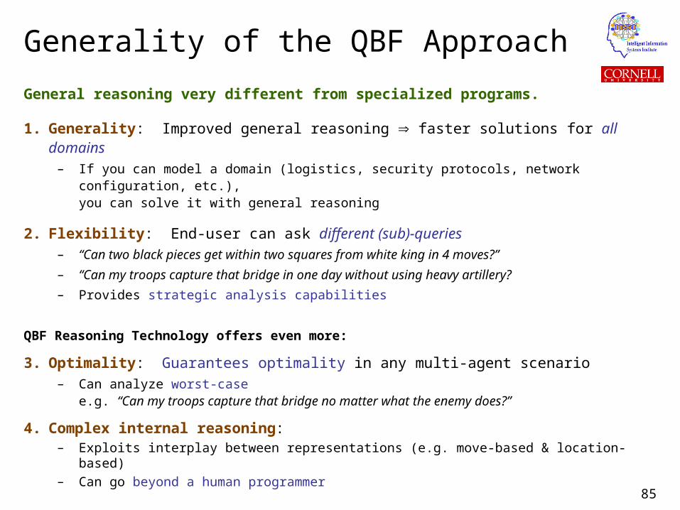
Generality of the QBF Approach
General reasoning very different from specialized programs.
1. Generality: Improved general reasoning faster solutions for all domains– If you can model a domain (logistics, security protocols, network configuration, etc.),
you can solve it with general reasoning
2. Flexibility: End-user can ask different (sub)-queries– “Can two black pieces get within two squares from white king in 4 moves?”
– “Can my troops capture that bridge in one day without using heavy artillery?
– Provides strategic analysis capabilities
QBF Reasoning Technology offers even more:
3. Optimality: Guarantees optimality in any multi-agent scenario– Can analyze worst-case
e.g. “Can my troops capture that bridge no matter what the enemy does?”
4. Complex internal reasoning: – Exploits interplay between representations (e.g. move-based & location-based)
– Can go beyond a human programmer
86
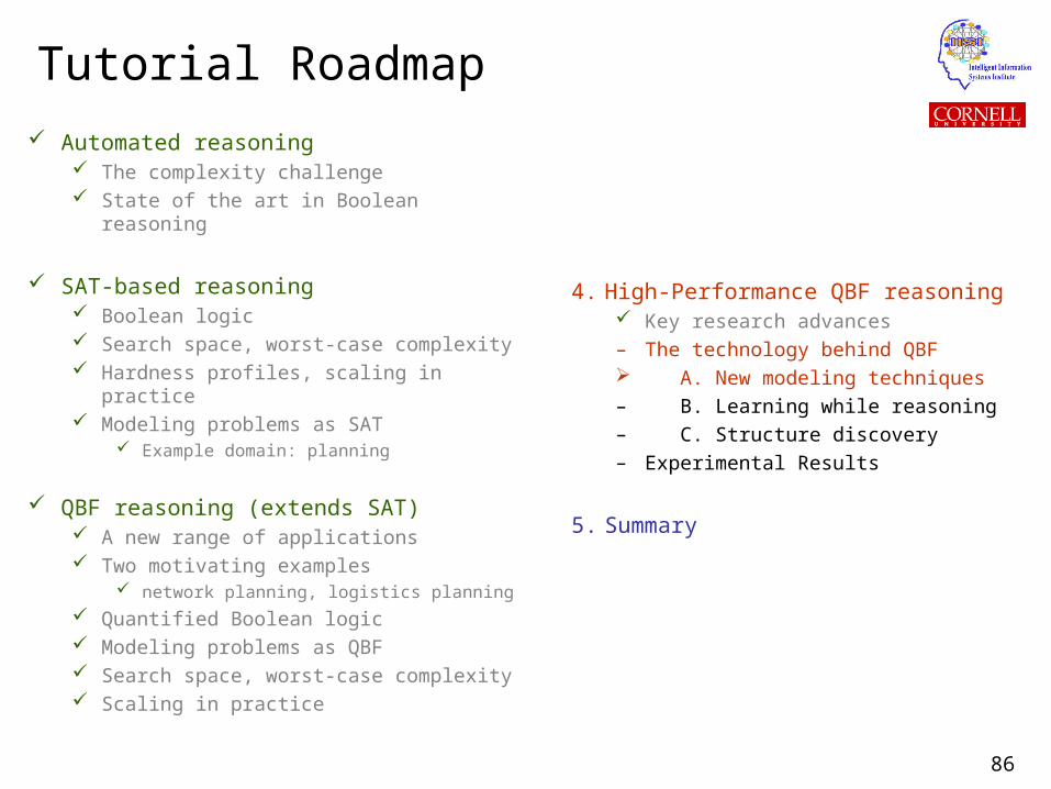
Tutorial Roadmap
Automated reasoning The complexity challenge State of the art in Boolean reasoning
SAT-based reasoning Boolean logic Search space, worst-case complexity Hardness profiles, scaling in practice Modeling problems as SAT
Example domain: planning
QBF reasoning (extends SAT) A new range of applications Two motivating examples
network planning, logistics planning
Quantified Boolean logic Modeling problems as QBF Search space, worst-case complexity Scaling in practice
4. High-Performance QBF reasoning Key research advances– The technology behind QBF A. New modeling techniques– B. Learning while reasoning– C. Structure discovery– Experimental Results
5. Summary
87
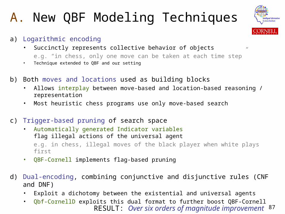
A. New QBF Modeling Techniques
a) Logarithmic encoding• Succinctly represents collective behavior of objects
e.g. “in chess, only one move can be taken at each time step”• Technique extended to QBF and our setting
b) Both moves and locations used as building blocks• Allows interplay between move-based and location-based reasoning / representation• Most heuristic chess programs use only move-based search
c) Trigger-based pruning of search space• Automatically generated Indicator variables
flag illegal actions of the universal agent
e.g. in chess, illegal moves of the black player when white plays first• QBF-Cornell implements flag-based pruning
d) Dual-encoding, combining conjunctive and disjunctive rules (CNF and DNF)• Exploit a dichotomy between the existential and universal agents• Qbf-CornellD exploits this dual format to further boost QBF-Cornell
RESULT: Over six orders of magnitude improvement
88
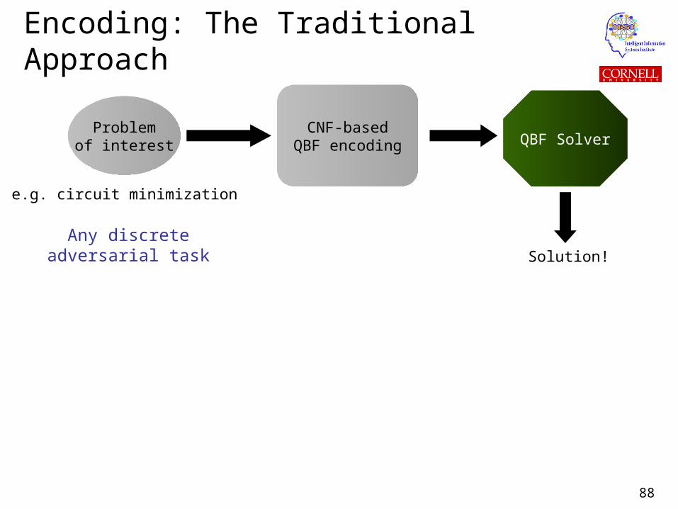
Encoding: The Traditional Approach
Problemof interest
e.g. circuit minimization
CNF-basedQBF encoding QBF Solver
Solution!Any discrete
adversarial task
89
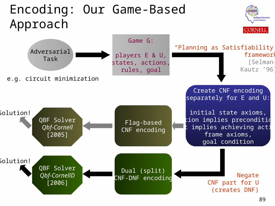
Encoding: Our Game-Based Approach
AdversarialTask
e.g. circuit minimization
Game G:
players E & U,states, actions,
rules, goal
“Planning as Satisfiability”framework
[Selman-Kautz ’96]
Create CNF encodingseparately for E and U:
initial state axioms,action implies precondition,
fact implies achieving action,frame axioms,goal condition
Dual (split)CNF-DNF encoding
QBF SolverQbf-CornellD
[2006]Negate
CNF part for U(creates DNF)
Solution!
Flag-basedCNF encoding
QBF SolverQbf-Cornell
[2005]
Solution!
96
Tutorial Roadmap
Automated reasoning The complexity challenge State of the art in Boolean reasoning
SAT-based reasoning Boolean logic Search space, worst-case complexity Hardness profiles, scaling in practice Modeling problems as SAT
Example domain: planning
QBF reasoning (extends SAT) A new range of applications Two motivating examples
network planning, logistics planning
Quantified Boolean logic Modeling problems as QBF Search space, worst-case complexity Scaling in practice
4. High-Performance QBF reasoning Key research advances– The technology behind QBF A. New modeling techniques B. Learning while reasoning– C. Structure discovery– Experimental Results
5. Summary
97
B. Learning while Reasoning
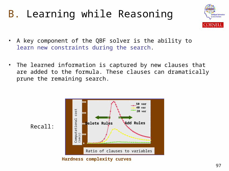
• A key component of the QBF solver is the ability to learn new constraints during the search.
• The learned information is captured by new clauses that are added to the formula. These clauses can dramatically prune the remaining search.
Com
pu
tati
onal
Cos
t
50 var
40 var
20 var
0
1000
3000
2000
4000
Ratio of clauses to variables
Computational cost
(secs)
Hardness complexity curves
Add RulesDelete RulesRecall:
98
Encoding: Before Learning
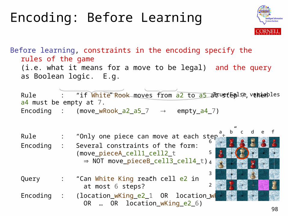
Before learning, constraints in the encoding specify the rules of the game(i.e. what it means for a move to be legal) and the query as Boolean logic. E.g.
Rule : “if White Rook moves from a2 to a5 at step 7, then a4 must be empty at 7.”Encoding : (move_wRook_a2_a5_7 empty_a4_7)
Rule : “Only one piece can move at each step t.”
Encoding : Several constraints of the form: (move_pieceA_cell1_cell2_t NOT move_pieceB_cell3_cell4_t)
Query : “Can White King reach cell e2 in at most 6 steps?”
Encoding : (location_wKing_e2_1 OR location_wKing_e2_2 OR … OR location_wKing_e2_6)
1
2
3
4
5
6
a b c d e f
True/False variables
99
Encoding: After Learning
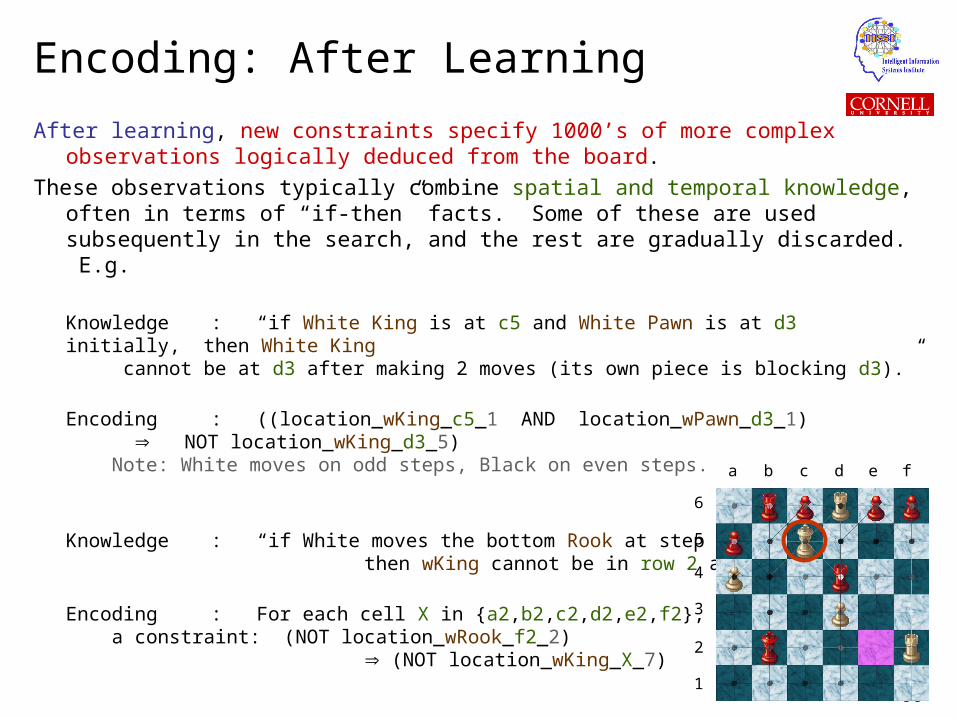
After learning, new constraints specify 1000’s of more complex observations logically deduced from the board.
These observations typically combine spatial and temporal knowledge, often in terms of “if-then” facts. Some of these are used subsequently in the search, and the rest are gradually discarded. E.g.
Knowledge : “if White King is at c5 and White Pawn is at d3 initially, then White King
cannot be at d3 after making 2 moves (its own piece is blocking d3).”
Encoding : ((location_wKing_c5_1 AND location_wPawn_d3_1) NOT location_wKing_d3_5) Note: White moves on odd steps, Black on even steps.
Knowledge : “if White moves the bottom Rook at step 1, then wKing cannot be in row 2 at step 7.”
Encoding : For each cell X in {a2,b2,c2,d2,e2,f2}, a constraint: (NOT location_wRook_f2_2) (NOT location_wKing_X_7) 1
2
3
4
5
6
a b c d e f
100
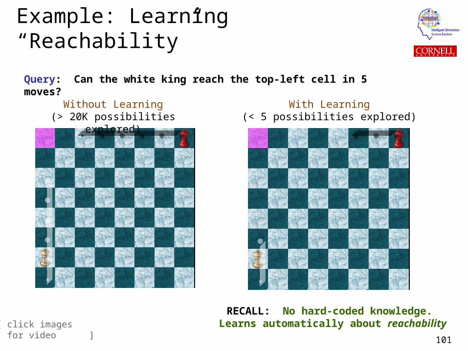
Learning while Reasoning
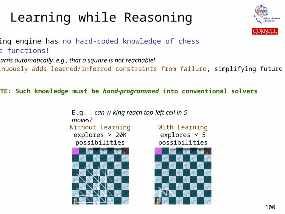
E.g. can w-king reach top-left cell in 5 moves?
Without Learningexplores > 20K
possibilities
With Learningexplores < 5possibilities
QBF reasoning engine has no hard-coded knowledge of chessor distance functions! – still learns automatically, e.g., that a square is not reachable! – continuously adds learned/inferred constraints from failure, simplifying future search
NOTE: Such knowledge must be hand-programmed into conventional solvers
101
[ click images for video ]
Query: Can the white king reach the top-left cell in 5 moves?
Without Learning(> 20K possibilities explored)
With Learning(< 5 possibilities explored)
RECALL: No hard-coded knowledge. Learns automatically about reachability
Example: Learning “Reachability”
102
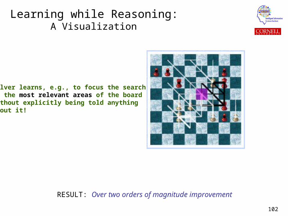
Learning while Reasoning: A Visualization
RESULT: Over two orders of magnitude improvement
Solver learns, e.g., to focus the searchto the most relevant areas of the boardwithout explicitly being told anythingabout it!
103
Tutorial Roadmap
Automated reasoning The complexity challenge State of the art in Boolean reasoning
SAT-based reasoning Boolean logic Search space, worst-case complexity Hardness profiles, scaling in practice Modeling problems as SAT
Example domain: planning
QBF reasoning (extends SAT) A new range of applications Two motivating examples
network planning, logistics planning
Quantified Boolean logic Modeling problems as QBF Search space, worst-case complexity Scaling in practice
4. High-Performance QBF reasoning Key research advances– The technology behind QBF A. New modeling techniques B. Learning while reasoning C. Structure discovery– Experimental Results
5. Summary
104
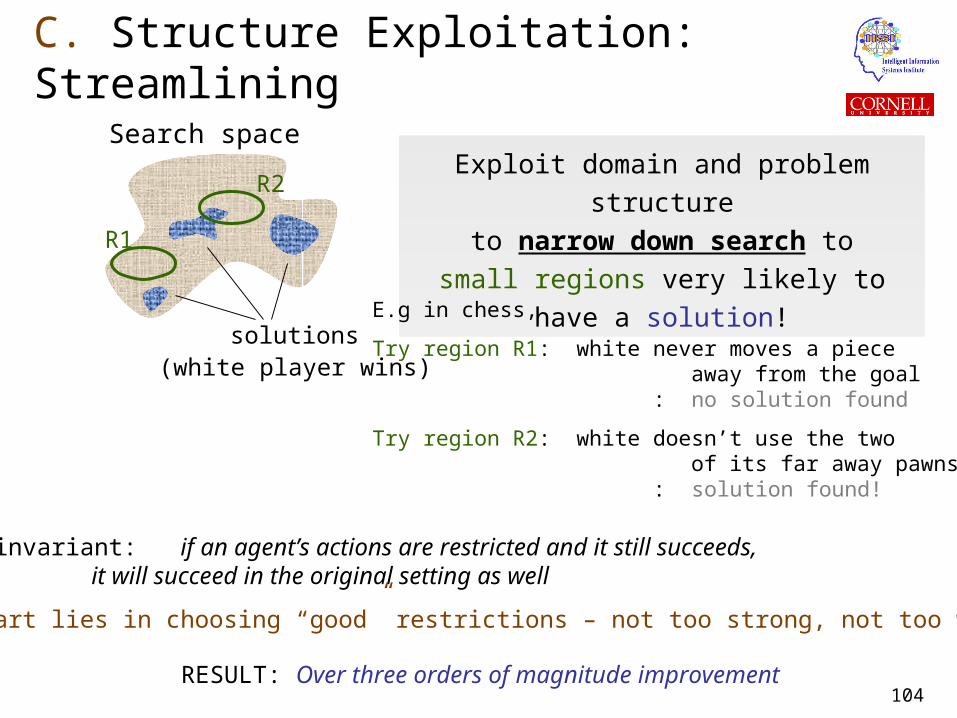
C. Structure Exploitation: Streamlining
Search space
solutions
Exploit domain and problem structure
to narrow down search to
small regions very likely to have a solution!
E.g in chess,
Try region R1: white never moves a piece away from the goal : no solution found
Try region R2: white doesn’t use the two of its far away pawns : solution found!
R1
R2
Key invariant: if an agent’s actions are restricted and it still succeeds, it will succeed in the original setting as well
The art lies in choosing “good” restrictions – not too strong, not too weak!
(white player wins)
RESULT: Over three orders of magnitude improvement
105
Structure Exploitation: Structure Discovery
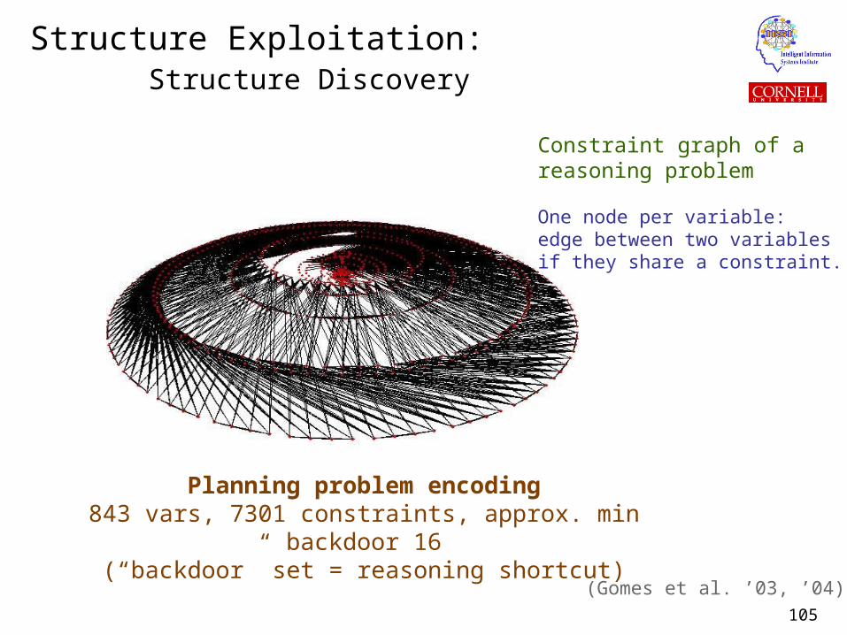
Planning problem encoding843 vars, 7301 constraints, approx. min backdoor 16
(“backdoor” set = reasoning shortcut)
Constraint graph of areasoning problem
One node per variable:edge between two variablesif they share a constraint.
(Gomes et al. ’03, ’04)
106
Structure Exploitation: Structure Discovery
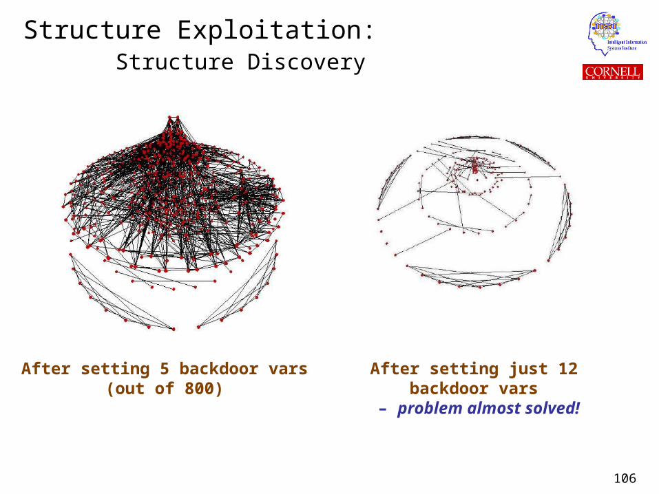
After setting 5 backdoor vars(out of 800)
After setting just 12 backdoor vars – problem almost solved!
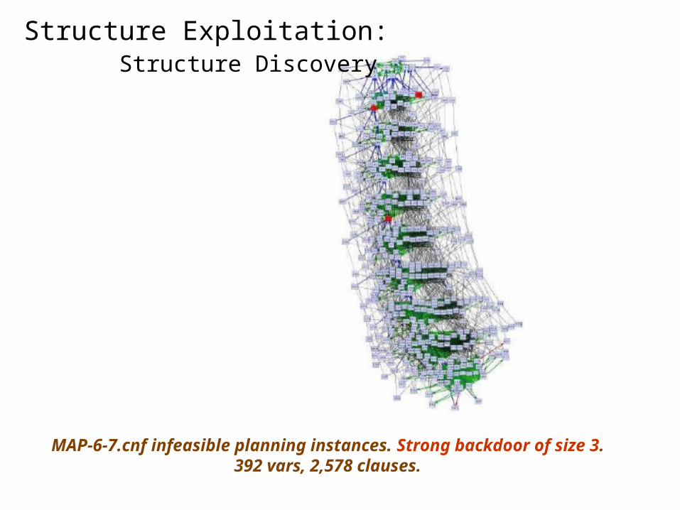
MAP-6-7.cnf infeasible planning instances. Strong backdoor of size 3.392 vars, 2,578 clauses.
Structure Exploitation: Structure Discovery
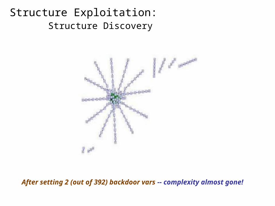
After setting 2 (out of 392) backdoor vars -- complexity almost gone!
Structure Exploitation: Structure Discovery
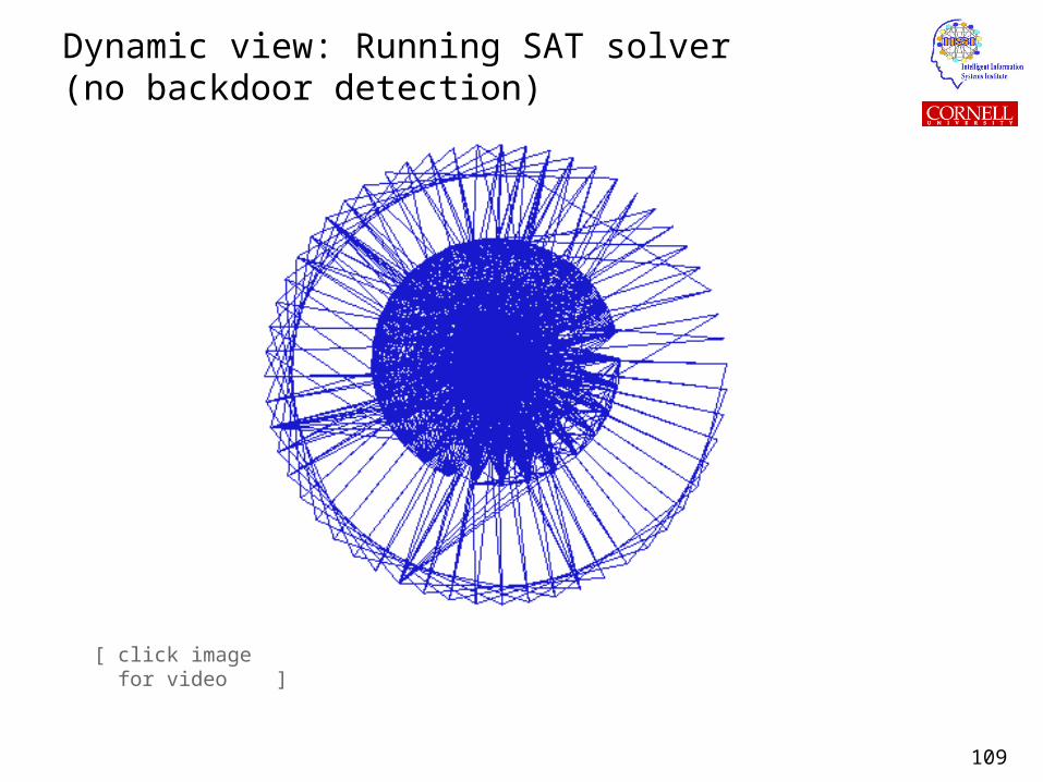
109
Dynamic view: Running SAT solver(no backdoor detection)
[ click image for video ]
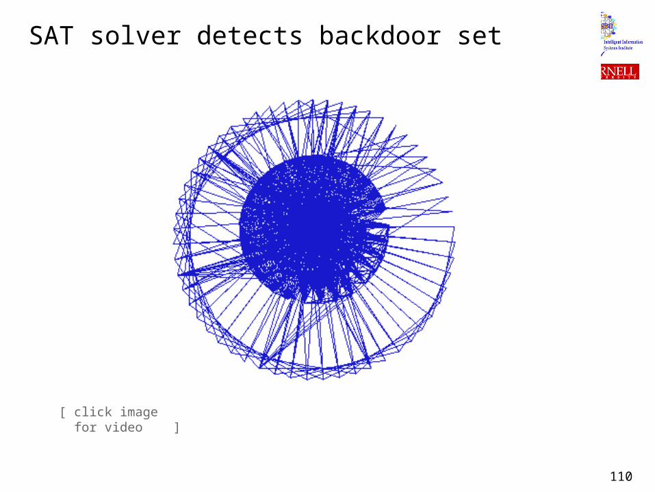
110
SAT solver detects backdoor set
[ click image for video ]
111
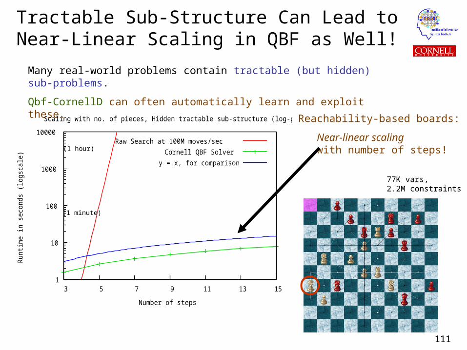
Tractable Sub-Structure Can Lead toNear-Linear Scaling in QBF as Well!
Many real-world problems contain tractable (but hidden) sub-problems.
Qbf-CornellD can often automatically learn and exploit these.
Reachability-based boards:
Near-linear scaling with number of steps!
1
10
100
1000
10000
3 5 7 9 11 13 15
Run
time
in s
econ
ds (l
ogsc
ale)
Number of steps
Scaling with no. of pieces, Hidden tractable sub-structure (log-plot)
Raw Search at 100M moves/secCornell QBF Solver
y = x, for comparison
(1 hour)
(1 minute)
77K vars,2.2M constraints
112
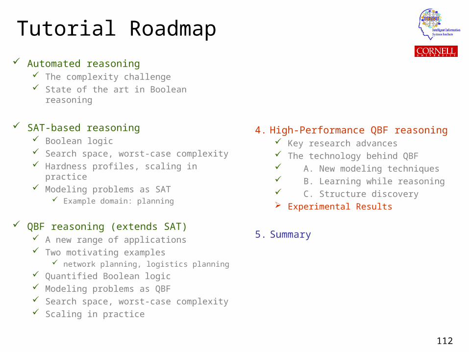
Tutorial Roadmap
Automated reasoning The complexity challenge State of the art in Boolean reasoning
SAT-based reasoning Boolean logic Search space, worst-case complexity Hardness profiles, scaling in practice Modeling problems as SAT
Example domain: planning
QBF reasoning (extends SAT) A new range of applications Two motivating examples
network planning, logistics planning
Quantified Boolean logic Modeling problems as QBF Search space, worst-case complexity Scaling in practice
4. High-Performance QBF reasoning Key research advances The technology behind QBF A. New modeling techniques B. Learning while reasoning C. Structure discovery Experimental Results
5. Summary
113
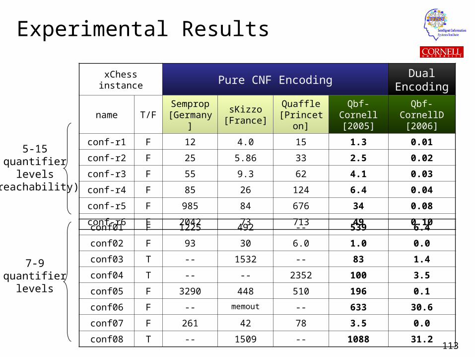
Experimental Results
xChess instance Pure CNF EncodingDual
Encoding
name T/FSemprop
[Germany]sKizzo
[France]Quaffle
[Princeton]Qbf-Cornell
[2005]Qbf-CornellD
[2006]
conf-r1 F 12 4.0 15 1.3 0.01
conf-r2 F 25 5.86 33 2.5 0.02
conf-r3 F 55 9.3 62 4.1 0.03
conf-r4 F 85 26 124 6.4 0.04
conf-r5 F 985 84 676 34 0.08
conf-r6 F 2042 73 713 49 0.10
conf01 F 1225 492 -- 539 6.4
conf02 F 93 30 6.0 1.0 0.0
conf03 T -- 1532 -- 83 1.4
conf04 T -- -- 2352 100 3.5
conf05 F 3290 448 510 196 0.1
conf06 F -- memout -- 633 30.6
conf07 F 261 42 78 3.5 0.0
conf08 T -- 1509 -- 1088 31.2
5-15quantifier
levels(reachability)
7-9quantifier
levels
114
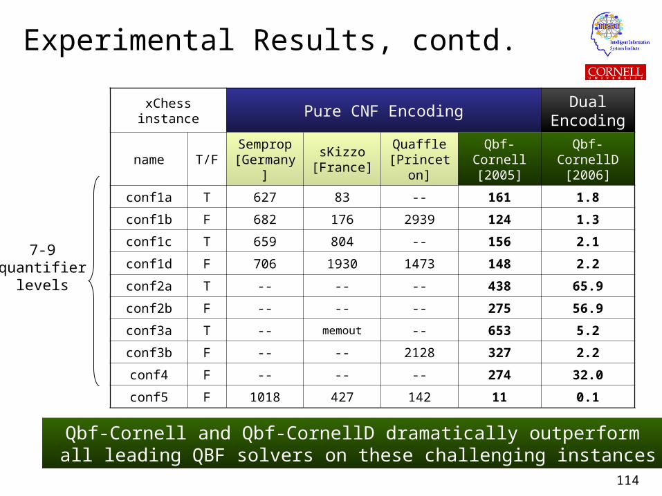
Experimental Results, contd.
xChess instance Pure CNF EncodingDual
Encoding
name T/FSemprop
[Germany]sKizzo
[France]Quaffle
[Princeton]Qbf-Cornell
[2005]Qbf-CornellD
[2006]
conf1a T 627 83 -- 161 1.8
conf1b F 682 176 2939 124 1.3
conf1c T 659 804 -- 156 2.1
conf1d F 706 1930 1473 148 2.2
conf2a T -- -- -- 438 65.9
conf2b F -- -- -- 275 56.9
conf3a T -- memout -- 653 5.2
conf3b F -- -- 2128 327 2.2
conf4 F -- -- -- 274 32.0
conf5 F 1018 427 142 11 0.1
7-9quantifier
levels
Qbf-Cornell and Qbf-CornellD dramatically outperform all leading QBF solvers on these challenging instances
115
Tutorial Roadmap
Automated reasoning The complexity challenge State of the art in Boolean reasoning
SAT-based reasoning Boolean logic Search space, worst-case complexity Hardness profiles, scaling in practice Modeling problems as SAT
Example domain: planning
QBF reasoning (extends SAT) A new range of applications Two motivating examples
network planning, logistics planning
Quantified Boolean logic Modeling problems as QBF Search space, worst-case complexity Scaling in practice
High-Performance QBF reasoning Key research advances The technology behind QBF A. New modeling techniques B. Learning while reasoning C. Structure discovery Experimental results
5. Summary
116
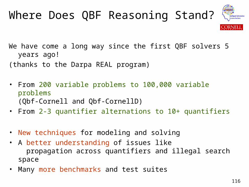
Where Does QBF Reasoning Stand?
We have come a long way since the first QBF solvers 5 years ago!
(thanks to the Darpa REAL program)
• From 200 variable problems to 100,000 variable problems(Qbf-Cornell and Qbf-CornellD)
• From 2-3 quantifier alternations to 10+ quantifiers
• New techniques for modeling and solving• A better understanding of issues like
propagation across quantifiers and illegal search space• Many more benchmarks and test suites
117
Summary
QBF Reasoning: a promising new automated reasoning technology!
On the road to a whole new range of applications:
• Strategic decision making
• Performance guarantees in complex multi-agent scenarios
• Secure communication and data networks in hostile environments
• Robust logistics planning in adversarial settings
• Large scale contingency planning
• Provably robust and secure software and hardware
118
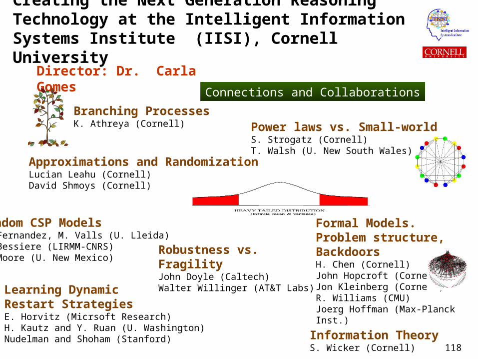
Formal Models. Problem structure, BackdoorsH. Chen (Cornell)John Hopcroft (Cornell)Jon Kleinberg (Cornell)R. Williams (CMU)Joerg Hoffman (Max-Planck Inst.)
Creating the Next Generation ReasoningTechnology at the Intelligent Information Systems Institute (IISI), Cornell University
Information TheoryS. Wicker (Cornell)
Branching ProcessesK. Athreya (Cornell)
Robustness vs.FragilityJohn Doyle (Caltech)Walter Willinger (AT&T Labs)
Power laws vs. Small-world S. Strogatz (Cornell)T. Walsh (U. New South Wales)
Director: Dr. Carla Gomes
Learning Dynamic Restart StrategiesE. Horvitz (Micrsoft Research)H. Kautz and Y. Ruan (U. Washington)Nudelman and Shoham (Stanford)
Random CSP ModelsC. Fernandez, M. Valls (U. Lleida)C. Bessiere (LIRMM-CNRS)C. Moore (U. New Mexico)
Connections and Collaborations
Approximations and RandomizationLucian Leahu (Cornell)David Shmoys (Cornell)
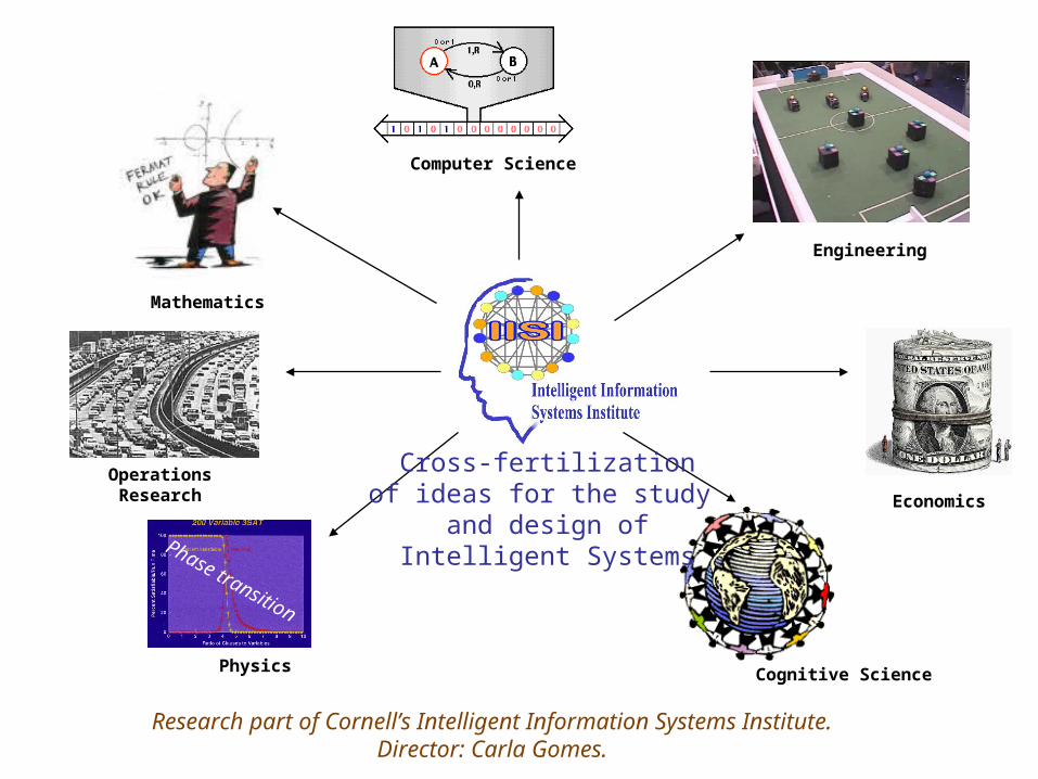
Computer Science
Mathematics
Operations Research
Physics Cognitive Science
Economics
Cross-fertilizationof ideas for the study
and design ofIntelligent SystemsPhase transition
Engineering
Research part of Cornell’s Intelligent Information Systems Institute.Director: Carla Gomes.

Additional Material
121
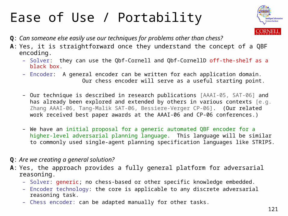
Ease of Use / Portability
Q: Can someone else easily use our techniques for problems other than chess?A: Yes, it is straightforward once they understand the concept of a QBF encoding.
– Solver: they can use the Qbf-Cornell and Qbf-CornellD off-the-shelf as a black box.
– Encoder: A general encoder can be written for each application domain. Our chess encoder will serve as a useful starting point.
– Our technique is described in research publications [AAAI-05, SAT-06] and has already been explored and extended by others in various contexts [e.g. Zhang AAAI-06, Tang-Malik SAT-06, Bessiere-Verger CP-06]. (Our related work received best paper awards at the AAAI-06 and CP-06 conferences.)
– We have an initial proposal for a generic automated QBF encoder for a higher-level adversarial planning language. This language will be similar to commonly used single-agent planning specification languages like STRIPS.
Q: Are we creating a general solution?A: Yes, the approach provides a fully general platform for adversarial reasoning.
– Solver: generic; no chess-based or other specific knowledge embedded.– Encoder technology: the core is applicable to any discrete adversarial reasoning task.– Chess encoder: can be adapted manually for other tasks.
122
Encoding: Generation
• The encoding process is automatic and very efficient.– The “encoding” is a re-statement of the problem in the language of the solver.– We use a fully automated chess-to-QBF encoder.– Each of the 600 go/no-go boards required < 0.3 sec to encode.– The hardest instances we have tried required < 2 sec to encode.– For chess and most future applications of interest, encoder time will be polynomial in
the problem parameters. The challenge is always the solver time.
The encoding process takes a fraction of the time compared to the solver.
123
Encoding: Effect of Number of Steps
The number of steps is simply a parameter to the encoder.
If a different number of steps is desired, the new encoding can be generated within seconds by re-running the encoder.
Additional information:– Decreasing the number of steps (and possibly also changing the query itself) :
Requires changing only the few constraints that encode the new query (< 1% of the encoding). The rest of the encoding (> 99%) remains
untouched.
– Increasing the number of steps in the query: Requires additional variables and constraints for the extra steps,
which are simply appended to the original encoding.
– Transfer learning technology can be exploited to re-use knowledge gained from the original encoding when the query is changed; we are exploring this.
124
From Adversarial Tasks To Games
Example #2:
The Chromatic Number Problem: Given a graph G and a positive number k, does G have chromatic number k?– Chromatic number: minimum number of colors needed to color G so
that every two adjacent vertices get different colors
– A game with 2 turns• Moves : First, E produces a coloring S of G; second, U
produces a coloring T of G
• Rules : S must be a legal k-coloring of G; T must be a legal
(k-1)-coloring of G
• Goal : E wins if S is valid and T is not
– “E wins” iff graph G has chromatic number k