AUTHORS

Creties Jenkins � DeGolyer and MacNaughton,Dallas, Texas; cjenkins@demac.com

Creties Jenkins is a senior staff geologist for De-Golyer and MacNaughton where he specializesin reservoir characterization, geocellular modeling,and resource estimation in clastic reservoirs, in-

Quantifying and predictingnaturally fractured reservoirbehavior with continuousfracture models

cluding coalbed methane and shale gas accumu-lations. He received an M.S. degree in geology anda B.S. degree in geological engineering from the

Creties Jenkins, Ahmed Ouenes, Abdel Zellou, and South Dakota School of Mines and Technology. Jeff Wingard

Ahmed Ouenes � Prism Seismic, GreenwoodVillage, Colorado; ouenes@prismseismic.com

Ahmed Ouenes is the president of Prism Seismic.Previously, he was the chief reservoir engineer at(RC)2 where he developed the first commercialsoftware for the CFM technology. Ahmed’s maininterest is the development of improved reservoircharacterization technologies especially for frac-tured reservoirs. Ahmed graduated from EcoleCentrale de Paris and holds a Ph.D. in petroleumengineering from New Mexico Tech.

Abdel Zellou � Prism Seismic, Centennial,Colorado; abdel@prismseismic.com

Abdel M. Zellou is director of consulting at PrismSeismic. He has worked as a consultant on nu-merous fractured reservoirs all over the worldand contributed to the drilling of many successfulwells. He codeveloped ReFract, a leading frac-tured reservoir software using patented technology.Abdel graduated from New Mexico Tech with anM.Sc. degree in petroleum engineering.

Jeff Wingard � DeGolyer and MacNaughton,Dallas, Texas; jwingard@demac.com

ABSTRACT

This article describes the workflow used in continuous fracturemodeling (CFM) and its successful application to several projects.Our CFM workflow consists of four basic steps: (1) interpreting keyseismic horizons and generating prestack and poststack seismic attri-butes; (2) using these attributes along with log and core data to buildseismically constrained geocellularmodels of lithology, porosity, watersaturation, etc.; (3) combining the derived geocellular models withprestack and poststack seismic attributes and additional geomechan-ical models to derive high-resolution three-dimensional (3-D) fracturemodels; and (4) validating the 3-D fracture models in a dynamic res-ervoir simulator by testing their ability to match well performance.

Our CFMworkflow uses a neural network approach to integrateall of the available static and dynamic data. This results in a modelthat is better able to identify fractured areas and quantify their im-pact on well and reservoir flow behavior. This technique has beensuccessfully applied in numerous sandstone and carbonate reservoirsto both understand reservoir behavior and determine where to drilladditional wells. Three field case studies are used to illustrate thecapabilities of the CFM approach.

Jeff Wingard is a senior staff reservoir engineer atDeGolyer and MacNaughton where he has devel-oped and evaluated geocellular and simulationmodels for waterflood, miscible gas, and thermalEnhanced Oil Recovery projects. He earned a B.S.degree in chemical engineering from the Massa-chusetts Institute of Technology in 1980 and a Ph.D.in petroleum engineering from Stanford Universityin 1988.

INTRODUCTION

The characterization of naturally fractured reservoirs is a recurringchallenge for oil and gas companies. Reservoir models built to assistwith field development planning and depletion optimization need toaccurately incorporate the effects of natural fractures in the near-wellbore regions and to also predict their distribution in interwellareas.

ACKNOWLEDGEMENTS

The AAPG Editor thanks the following reviewersfor their work on this paper: Soren Christensen,Stuart D. Harker, Tony Morland, Ronald A. Nelson,and an anonymous reviewer.

Copyright ©2009. The American Association of Petroleum Geologists. All rights reserved.

Manuscript received February 10, 2009; provisional acceptance April 16, 2009; revised manuscriptreceived May 31, 2009; final acceptance July 13, 2009.DOI:10.1306/07130909016

AAPG Bulletin, v. 93, no. 11 (November 2009), pp. 1597– 1608 1597

Many attempts have beenmade in the past to achievethis, but most of them have proven to be inaccurate andunreliable. For example, many companies are still usingsimple methods such as reservoir curvature to identifyareas that are likely to be fractured. Such a simplified ap-proach ignores lithology, bed thickness, and other factorsthat are generally known to influence fracture develop-ment. Similarly, geostatistical techniques such as krigingand sequential Gaussian simulation (SGS) are commonlyinadequate for distributing fracture properties in inter-well areas because these properties do not change in aregular manner away from well control.

Geomechanical models attempt to construct a frac-ture description and mechanical property distributionfrom the tectonic history, but these models commonlyfail to capture the complex heterogeneity and anisotro-py of the fracture system (Mace et al., 2004). Discretefracture modeling (Dershowitz et al., 1998; Sabathieret al., 1998), which has become very popular in recentyears, is constrained by the assumption that a limitednumber of macroscale fractures, as observed in coresand image logs, control fluid flow. A review of discretefracture modeling methods and their characteristics canbe found in the works of Dershowitz et al. (2004) andBourbiaux et al. (2005).

To capture fracture effects at multiple scales andsimultaneously integrate all of the available information,including core, log, seismic, and well test data, an alter-native technique (Ouenes et al., 1995; Ouenes, 2000)called continuous fracture modeling (CFM) can be used.

This article provides a review of the CFM approachby describing its key characteristics and illustrating thesewith three case studies. In each of these studies, objec-tive criteria are used to evaluate the predictive capabil-ity of the generated model, which is critical to ensure itsreliability. This can be done by comparing the modelproperties to the actual properties found in new wellsor in existing wells that were not used to construct themodel (also known as blind wells). Another method ofcomparison is to test the validity of themodel in a numer-ical simulator to see if well performance can be reason-ably matched without significant model adjustments.

CONTINUOUS FRACTURE MODELING APPROACH

The CFM approach does not focus on the fracturesthemselves but instead on the factors that control wherefracturing occurs. Lithology, structure, proximity to faults,

1598 Continuous Fracture Modeling (CFM)

and other geological factors are commonly known tocontrol the location and intensity of fracturing. Thesefactors, known as fracture drivers, can be identifiednot just from wellbore data but also from seismic data,which is the key to predicting fracture occurrencethroughout the reservoir. Through the CFM approach,these fracture drivers are related to fracture indicators,which include the interpretation of fractures from coredescriptions, image logs, and production logs that dem-onstrate the existence of a fracture at a specific location.Once this relationship is established, the fracture driv-ers can be used to predict the location of fractures else-where in the reservoir.

Common geological fracture drivers include faciestypes, porosity, and reservoir zonation. Geomechanicalfracture drivers include deformation, slopes and curva-tures of structural surfaces in multiple directions, andproximity to faults. Seismic fracture drivers include elas-tic properties, acoustic impedance, and spectral imagingattributes. In combination, these fracture drivers are amuchmore powerful tool for characterizing the fracturesystem than if used alone.

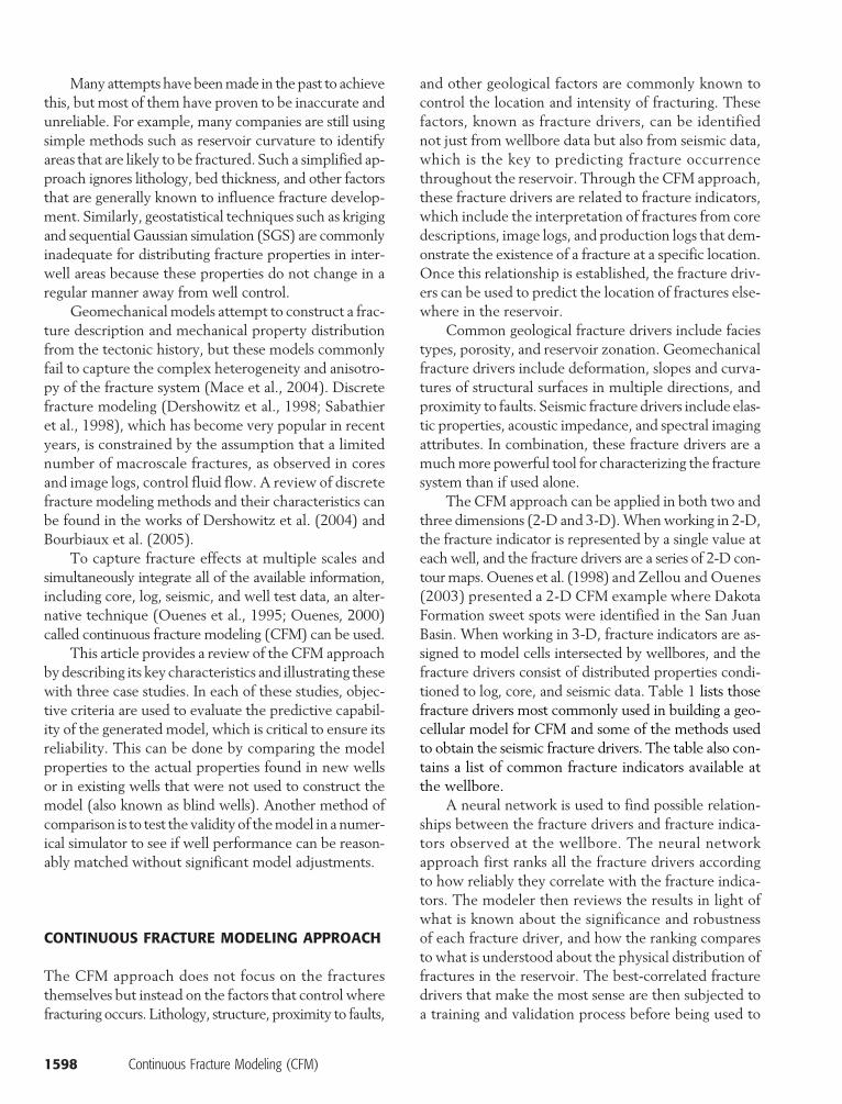
The CFM approach can be applied in both two andthree dimensions (2-D and 3-D).Whenworking in 2-D,the fracture indicator is represented by a single value ateach well, and the fracture drivers are a series of 2-D con-tourmaps.Ouenes et al. (1998) and Zellou and Ouenes(2003) presented a 2-D CFM example where DakotaFormation sweet spots were identified in the San JuanBasin. When working in 3-D, fracture indicators are as-signed to model cells intersected by wellbores, and thefracture drivers consist of distributed properties condi-tioned to log, core, and seismic data. Table 1 lists thosefracture drivers most commonly used in building a geo-cellular model for CFM and some of the methods usedto obtain the seismic fracture drivers. The table also con-tains a list of common fracture indicators available atthe wellbore.

A neural network is used to find possible relation-ships between the fracture drivers and fracture indica-tors observed at the wellbore. The neural networkapproach first ranks all the fracture drivers accordingto how reliably they correlate with the fracture indica-tors. The modeler then reviews the results in light ofwhat is known about the significance and robustnessof each fracture driver, and how the ranking comparesto what is understood about the physical distribution offractures in the reservoir. The best-correlated fracturedrivers that make the most sense are then subjected toa training and validation process before being used to

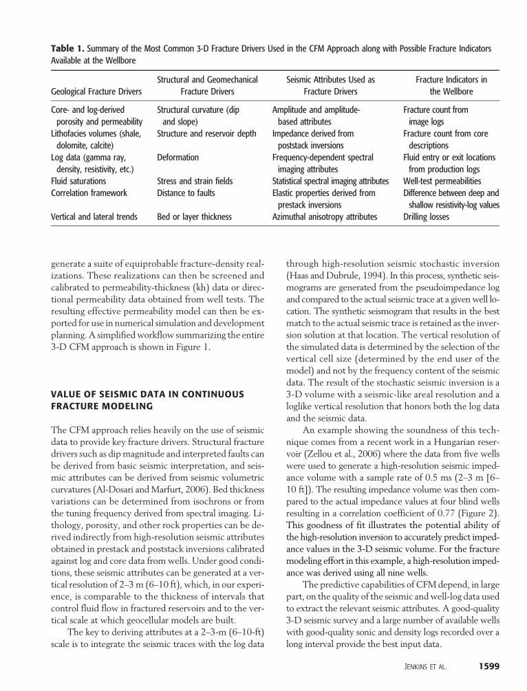
generate a suite of equiprobable fracture-density real-izations. These realizations can then be screened andcalibrated to permeability-thickness (kh) data or direc-tional permeability data obtained from well tests. Theresulting effective permeability model can then be ex-ported for use in numerical simulation and developmentplanning. A simplifiedworkflow summarizing the entire3-D CFM approach is shown in Figure 1.

VALUE OF SEISMIC DATA IN CONTINUOUSFRACTURE MODELING

The CFM approach relies heavily on the use of seismicdata to provide key fracture drivers. Structural fracturedrivers such as dipmagnitude and interpreted faults canbe derived from basic seismic interpretation, and seis-mic attributes can be derived from seismic volumetriccurvatures (Al-Dosari andMarfurt, 2006). Bed thicknessvariations can be determined from isochrons or fromthe tuning frequency derived from spectral imaging. Li-thology, porosity, and other rock properties can be de-rived indirectly from high-resolution seismic attributesobtained in prestack and poststack inversions calibratedagainst log and core data from wells. Under good condi-tions, these seismic attributes can be generated at a ver-tical resolution of 2–3m (6–10 ft), which, in our experi-ence, is comparable to the thickness of intervals thatcontrol fluid flow in fractured reservoirs and to the ver-tical scale at which geocellular models are built.

The key to deriving attributes at a 2–3-m (6–10-ft)scale is to integrate the seismic traces with the log data

through high-resolution seismic stochastic inversion(Haas and Dubrule, 1994). In this process, synthetic seis-mograms are generated from the pseudoimpedance logand compared to the actual seismic trace at a givenwell lo-cation. The synthetic seismogram that results in the bestmatch to the actual seismic trace is retained as the inver-sion solution at that location. The vertical resolution ofthe simulated data is determined by the selection of thevertical cell size (determined by the end user of themodel) and not by the frequency content of the seismicdata. The result of the stochastic seismic inversion is a3-D volume with a seismic-like areal resolution and aloglike vertical resolution that honors both the log dataand the seismic data.

An example showing the soundness of this tech-nique comes from a recent work in a Hungarian reser-voir (Zellou et al., 2006) where the data from five wellswere used to generate a high-resolution seismic imped-ance volume with a sample rate of 0.5 ms (2–3 m [6–10 ft]). The resulting impedance volume was then com-pared to the actual impedance values at four blind wellsresulting in a correlation coefficient of 0.77 (Figure 2).This goodness of fit illustrates the potential ability ofthe high-resolution inversion to accurately predict imped-ance values in the 3-D seismic volume. For the fracturemodeling effort in this example, a high-resolution imped-ance was derived using all nine wells.

The predictive capabilities of CFMdepend, in largepart, on the quality of the seismic andwell-log data usedto extract the relevant seismic attributes. A good-quality3-D seismic survey and a large number of available wellswith good-quality sonic and density logs recorded over along interval provide the best input data.

Table 1. Summary of the Most Common 3-D Fracture Drivers Used in the CFM Approach along with Possible Fracture Indicators

Available at the Wellbore

Geological Fracture Drivers

Structural and Geomechanical

Fracture Drivers

Seismic Attributes Used as

Fracture Drivers

Fracture Indicators in

the Wellbore

Core- and log-derivedporosity and permeability

Structural curvature (dipand slope)

Amplitude and amplitude-based attributes

Fracture count fromimage logs

Lithofacies volumes (shale,dolomite, calcite)

Structure and reservoir depth

Impedance derived frompoststack inversions

Fracture count from coredescriptions

Log data (gamma ray,density, resistivity, etc.)

Deformation

Frequency-dependent spectralimaging attributes

Fluid entry or exit locationsfrom production logs

Fluid saturations

Stress and strain fields Statistical spectral imaging attributes Well-test permeabilities Correlation framework Distance to faults Elastic properties derived from

prestack inversions

Difference between deep andshallow resistivity-log values

Vertical and lateral trends

Bed or layer thickness Azimuthal anisotropy attributes Drilling losses

Jenkins et al. 1599

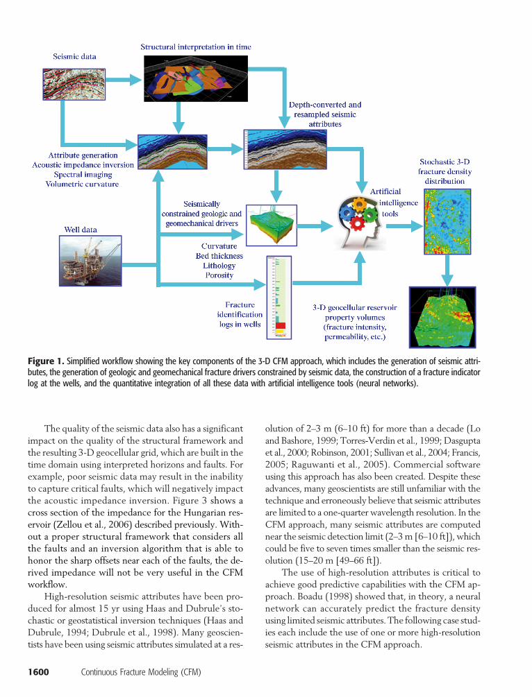
The quality of the seismic data also has a significantimpact on the quality of the structural framework andthe resulting 3-D geocellular grid, which are built in thetime domain using interpreted horizons and faults. Forexample, poor seismic data may result in the inabilityto capture critical faults, which will negatively impactthe acoustic impedance inversion. Figure 3 shows across section of the impedance for the Hungarian res-ervoir (Zellou et al., 2006) described previously. With-out a proper structural framework that considers allthe faults and an inversion algorithm that is able tohonor the sharp offsets near each of the faults, the de-rived impedance will not be very useful in the CFMworkflow.

High-resolution seismic attributes have been pro-duced for almost 15 yr using Haas and Dubrule’s sto-chastic or geostatistical inversion techniques (Haas andDubrule, 1994; Dubrule et al., 1998). Many geoscien-tists have been using seismic attributes simulated at a res-

1600 Continuous Fracture Modeling (CFM)

olution of 2–3 m (6–10 ft) for more than a decade (Loand Bashore, 1999; Torres-Verdin et al., 1999; Dasguptaet al., 2000; Robinson, 2001; Sullivan et al., 2004; Francis,2005; Raguwanti et al., 2005). Commercial softwareusing this approach has also been created. Despite theseadvances, many geoscientists are still unfamiliar with thetechnique and erroneously believe that seismic attributesare limited to a one-quarter wavelength resolution. In theCFM approach, many seismic attributes are computednear the seismic detection limit (2–3m [6–10 ft]), whichcould be five to seven times smaller than the seismic res-olution (15–20 m [49–66 ft]).

The use of high-resolution attributes is critical toachieve good predictive capabilities with the CFM ap-proach. Boadu (1998) showed that, in theory, a neuralnetwork can accurately predict the fracture densityusing limited seismic attributes. The following case stud-ies each include the use of one or more high-resolutionseismic attributes in the CFM approach.

Figure 1. Simplified workflow showing the key components of the 3-D CFM approach, which includes the generation of seismic attri-butes, the generation of geologic and geomechanical fracture drivers constrained by seismic data, the construction of a fracture indicatorlog at the wells, and the quantitative integration of all these data with artificial intelligence tools (neural networks).

FIELD CASE STUDIES OF CONTINUOUSFRACTURE MODELING

South Arne Chalk Field, Danish North Sea

In this project (Christensen et al., 2006), the CFM ap-proach was used to predict the 3-D distribution of frac-

ture density and to create reservoir simulation modelsin the South Arne field, a complex chalk reservoir. Nu-merous fracture drivers, including a high-resolutionacoustic impedance inversion and several spectral imag-ing attributes, were combined with porosity log valuesat 15 wells to construct a porosity model. The result-ing model compared very favorably with three blind

Figure 2. Predicted(x axis) versus actual (y axis)impedance at four blindwells not used in a seismicinversion. The predictedimpedance at the wellswas extracted from an im-pedance cube computedwith a resolution of 0.5 msor 2–3 m (6–10 ft) andcompared to the actuallogs averaged at 2 m (fromZellou et al., 2006; re-printed by permission ofthe Society of PetroleumEngineers).

Je

Figure 3. Cross sectionalong an inline showingthe derived impedance ata resolution of 0.5 ms. Be-cause the structural in-terpretation captures theexisting faults and theirsharp offsets, the derivedseismic attributes are morerepresentative and there-fore will be more usefulin the CFM workflow (fromZellou et al., 2006; re-printed by permission ofthe Society of PetroleumEngineers).

nkins et al. 1601

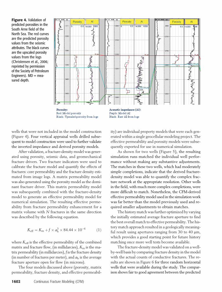
wells that were not included in the model construction(Figure 4). Four vertical appraisal wells drilled subse-quent to model construction were used to further validatethe inverted impedance and derived porosity models.

After validation, a fracture-densitymodel was gener-ated using porosity, seismic data, and geomechanicalfracture drivers. Two fracture indicators were used tocalibrate the fracture model and quantify the effects offractures: core permeability and the fracture density esti-mated from image logs. A matrix permeability modelwas also generated using the porosity model as the domi-nant fracture driver. This matrix permeability modelwas subsequently combined with the fracture-densitymodel to generate an effective permeability model fornumerical simulation. The resulting effective perme-ability from fracture permeability enhancement for amatrix volume with N fractures in the same directionwas described by the following equation.

Keff ¼ Km þ f � a3h � 84:44� 10�6 ð1Þ

where Keff is the effective permeability of the combinedmatrix and fracture flow, (in millidarcies), Km is the ma-trix permeability (inmillidarcies), f is the fracture density(in number of fractures per meter), and ah is the averagefracture aperture open for flow (in microns).

The four models discussed above (porosity, matrixpermeability, fracture density, and effective permeabil-

1602 Continuous Fracture Modeling (CFM)

ity) are individual property models that were each gen-erated within a single geocellular modeling project. Theeffective permeability and porosity models were subse-quently exported for use in numerical simulation.

As shown for two wells (Figure 5), the resultingsimulation runs matched the individual well perfor-mance without making any substantive adjustments.The matches in these two wells, which had moderatelysimple completions, indicate that the derived fracture-density model was able to quantify the complex frac-ture network at the appropriate resolution. Other wellsin the field, withmuchmore complex completions, weremore difficult to match. Nonetheless, the CFM-derivedeffective permeabilitymodel used in the simulationworkwas far better than the model previously used and re-quired smaller adjustments to obtain matches.

Thehistorymatchwas further optimized by varyingthe initially estimated average fracture aperture to findthe best overallmatch to effective permeability. The his-torymatch approach resulted in a geologically meaning-ful result using apertures ranging from 30 to 40 mm,which provides a good starting point for future historymatching once more well tests become available.

The fracture-density model was validated on a well-by-well basis by comparing fracture density in themodelwith the actual counts of conductive fractures. The re-sults are shown in Figure 6 for three random horizontalwells that were available during the study. The compar-ison shows fair to good agreement between the predicted

Figure 4. Validation ofpredicted porosities in theSouth Arne field of theNorth Sea. The red curvesare the predicted porosityvalues from the seismicattributes. The black curvesare the upscaled porosityvalues from the logs(Christensen et al., 2006;reprinted by permissionof the Society of PetroleumEngineers). MD = mea-sured depth.

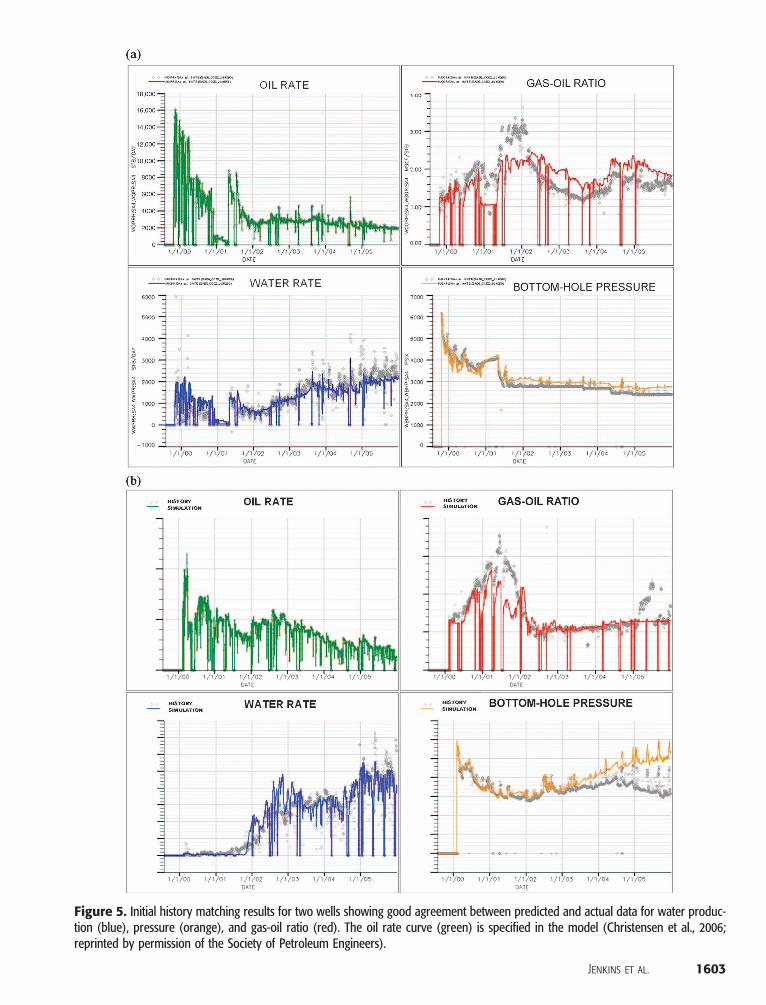
Figure 5. Initial history matching results for two wells showing good agreement between predicted and actual data for water produc-tion (blue), pressure (orange), and gas-oil ratio (red). The oil rate curve (green) is specified in the model (Christensen et al., 2006;reprinted by permission of the Society of Petroleum Engineers).

Jenkins et al. 1603

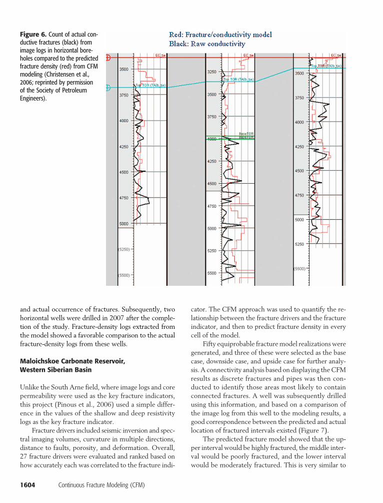
and actual occurrence of fractures. Subsequently, twohorizontal wells were drilled in 2007 after the comple-tion of the study. Fracture-density logs extracted fromthe model showed a favorable comparison to the actualfracture-density logs from these wells.

Maloichskoe Carbonate Reservoir,Western Siberian Basin

Unlike the South Arne field, where image logs and corepermeability were used as the key fracture indicators,this project (Pinous et al., 2006) used a simple differ-ence in the values of the shallow and deep resistivitylogs as the key fracture indicator.

Fracture drivers included seismic inversion and spec-tral imaging volumes, curvature in multiple directions,distance to faults, porosity, and deformation. Overall,27 fracture drivers were evaluated and ranked based onhow accurately each was correlated to the fracture indi-

1604 Continuous Fracture Modeling (CFM)

cator. The CFM approach was used to quantify the re-lationship between the fracture drivers and the fractureindicator, and then to predict fracture density in everycell of the model.

Fifty equiprobable fracturemodel realizations weregenerated, and three of these were selected as the basecase, downside case, and upside case for further analy-sis. A connectivity analysis based on displaying theCFMresults as discrete fractures and pipes was then con-ducted to identify those areas most likely to containconnected fractures. A well was subsequently drilledusing this information, and based on a comparison ofthe image log from this well to the modeling results, agood correspondence between the predicted and actuallocation of fractured intervals existed (Figure 7).

The predicted fracture model showed that the up-per interval would be highly fractured, themiddle inter-val would be poorly fractured, and the lower intervalwould be moderately fractured. This is very similar to

Figure 6. Count of actual con-ductive fractures (black) fromimage logs in horizontal bore-holes compared to the predictedfracture density (red) from CFMmodeling (Christensen et al.,2006; reprinted by permissionof the Society of PetroleumEngineers).

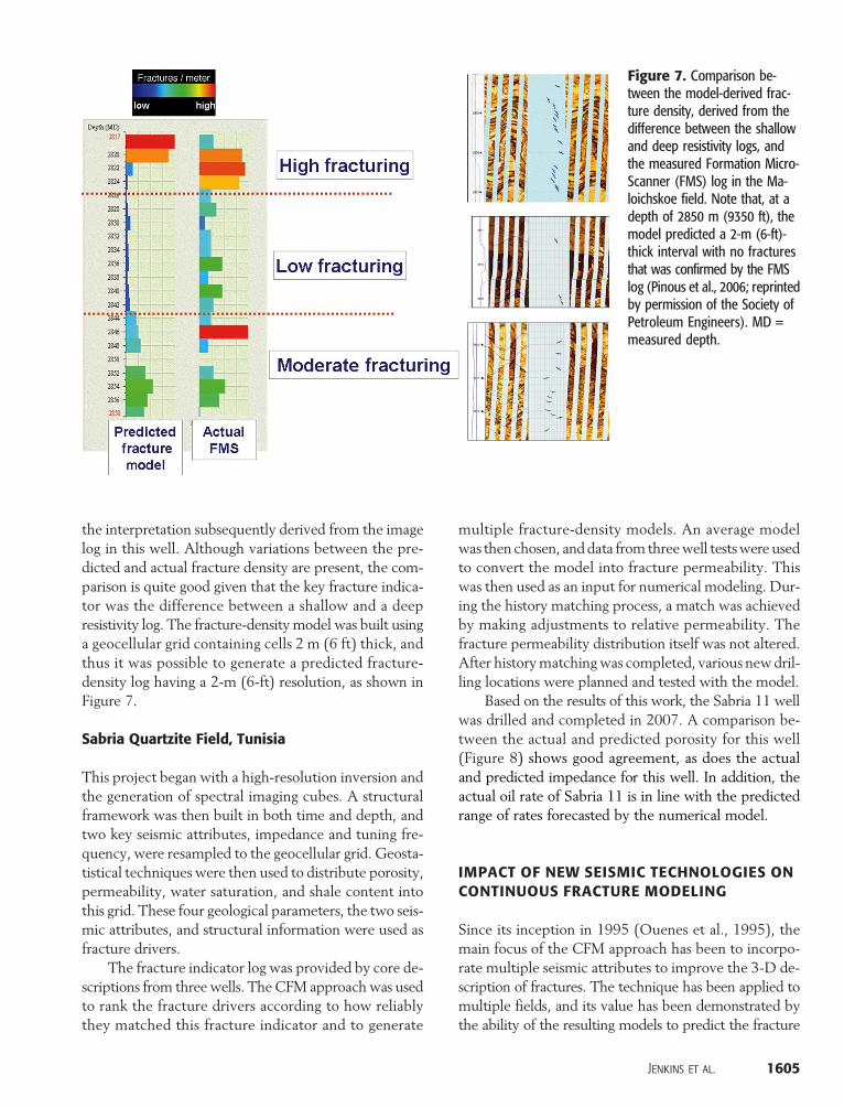
the interpretation subsequently derived from the imagelog in this well. Although variations between the pre-dicted and actual fracture density are present, the com-parison is quite good given that the key fracture indica-tor was the difference between a shallow and a deepresistivity log. The fracture-density model was built usinga geocellular grid containing cells 2 m (6 ft) thick, andthus it was possible to generate a predicted fracture-density log having a 2-m (6-ft) resolution, as shown inFigure 7.

Sabria Quartzite Field, Tunisia

This project began with a high-resolution inversion andthe generation of spectral imaging cubes. A structuralframework was then built in both time and depth, andtwo key seismic attributes, impedance and tuning fre-quency, were resampled to the geocellular grid. Geosta-tistical techniques were then used to distribute porosity,permeability, water saturation, and shale content intothis grid. These four geological parameters, the two seis-mic attributes, and structural information were used asfracture drivers.

The fracture indicator log was provided by core de-scriptions from three wells. TheCFM approachwas usedto rank the fracture drivers according to how reliablythey matched this fracture indicator and to generate

multiple fracture-density models. An average modelwas then chosen, anddata from threewell testswere usedto convert the model into fracture permeability. Thiswas then used as an input for numerical modeling. Dur-ing the history matching process, a match was achievedby making adjustments to relative permeability. Thefracture permeability distribution itself was not altered.After historymatchingwas completed, various newdril-ling locations were planned and tested with the model.

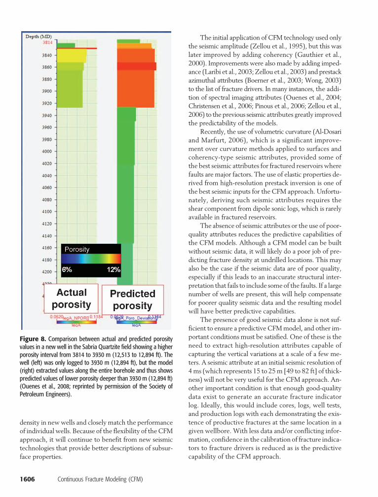
Based on the results of this work, the Sabria 11 wellwas drilled and completed in 2007. A comparison be-tween the actual and predicted porosity for this well(Figure 8) shows good agreement, as does the actualand predicted impedance for this well. In addition, theactual oil rate of Sabria 11 is in line with the predictedrange of rates forecasted by the numerical model.

IMPACT OF NEW SEISMIC TECHNOLOGIES ONCONTINUOUS FRACTURE MODELING

Since its inception in 1995 (Ouenes et al., 1995), themain focus of the CFM approach has been to incorpo-rate multiple seismic attributes to improve the 3-D de-scription of fractures. The technique has been applied tomultiple fields, and its value has been demonstrated bythe ability of the resulting models to predict the fracture

Figure 7. Comparison be-tween the model-derived frac-ture density, derived from thedifference between the shallowand deep resistivity logs, andthe measured Formation Micro-Scanner (FMS) log in the Ma-loichskoe field. Note that, at adepth of 2850 m (9350 ft), themodel predicted a 2-m (6-ft)-thick interval with no fracturesthat was confirmed by the FMSlog (Pinous et al., 2006; reprintedby permission of the Society ofPetroleum Engineers). MD =measured depth.

Jenkins et al. 1605

density in newwells and closely match the performanceof individual wells. Because of the flexibility of the CFMapproach, it will continue to benefit from new seismictechnologies that provide better descriptions of subsur-face properties.

1606 Continuous Fracture Modeling (CFM)

The initial application of CFM technology used onlythe seismic amplitude (Zellou et al., 1995), but this waslater improved by adding coherency (Gauthier et al.,2000). Improvements were also made by adding imped-ance (Laribi et al., 2003; Zellou et al., 2003) and prestackazimuthal attributes (Boerner et al., 2003; Wong, 2003)to the list of fracture drivers. In many instances, the addi-tion of spectral imaging attributes (Ouenes et al., 2004;Christensen et al., 2006; Pinous et al., 2006; Zellou et al.,2006) to the previous seismic attributes greatly improvedthe predictability of the models.

Recently, the use of volumetric curvature (Al-Dosariand Marfurt, 2006), which is a significant improve-ment over curvature methods applied to surfaces andcoherency-type seismic attributes, provided some ofthe best seismic attributes for fractured reservoirs wherefaults are major factors. The use of elastic properties de-rived from high-resolution prestack inversion is one ofthe best seismic inputs for the CFM approach. Unfortu-nately, deriving such seismic attributes requires theshear component from dipole sonic logs, which is rarelyavailable in fractured reservoirs.

The absence of seismic attributes or the use of poor-quality attributes reduces the predictive capabilities ofthe CFM models. Although a CFM model can be builtwithout seismic data, it will likely do a poor job of pre-dicting fracture density at undrilled locations. This mayalso be the case if the seismic data are of poor quality,especially if this leads to an inaccurate structural inter-pretation that fails to include some of the faults. If a largenumber of wells are present, this will help compensatefor poorer quality seismic data and the resulting modelwill have better predictive capabilities.

The presence of good seismic data alone is not suf-ficient to ensure a predictive CFMmodel, and other im-portant conditions must be satisfied. One of these is theneed to extract high-resolution attributes capable ofcapturing the vertical variations at a scale of a few me-ters. A seismic attribute at an initial seismic resolution of4ms (which represents 15 to 25m [49 to 82 ft] of thick-ness) will not be very useful for the CFM approach. An-other important condition is that enough good-qualitydata exist to generate an accurate fracture indicatorlog. Ideally, this would include cores, logs, well tests,and production logs with each demonstrating the exis-tence of productive fractures at the same location in agiven wellbore. With less data and/or conflicting infor-mation, confidence in the calibration of fracture indica-tors to fracture drivers is reduced as is the predictivecapability of the CFM approach.

Figure 8. Comparison between actual and predicted porosityvalues in a new well in the Sabria Quartzite field showing a higherporosity interval from 3814 to 3930 m (12,513 to 12,894 ft). Thewell (left) was only logged to 3930 m (12,894 ft), but the model(right) extracted values along the entire borehole and thus showspredicted values of lower porosity deeper than 3930 m (12,894 ft)(Ouenes et al., 2008; reprinted by permission of the Society ofPetroleum Engineers).

SUMMARY

A successful modeling approach for naturally fracturedreservoirs needs to predict where naturally fracturedintervals will be encountered in undrilled wells anddo so at a scale (2–3 m [6–10 ft]) that is comparableto core, log, and well-test data. A successful approachmust also be able to provide an effective permeabilitymodel for numerical simulation that will match the per-formance of individual wells.

The CFM approach meets these criteria based onthe results of multiple case studies. The approach pro-vides a method for geoscientists to quantitatively inte-grate all of the available data by simultaneously relatingmultiple fracture drivers to any type of fracture indica-tor. This integration is achieved by the quantitative andsimultaneous use of multiple 3-D property volumes,especially seismic attributes, to predict the interwelloccurrence of fractures and build effective permeabil-ity models that incorporate them.

As new seismic processing and interpretation tech-nologies continue to evolve, the resulting seismic attri-butes will be used to further improve the ability of theCFM approach to quantify the location and effects offractures on well performance.

REFERENCES CITED

Al-Dosari, S., and K. Marfurt, 2006, 3D volumetric multispectral es-timates of reflector curvature and rotation: Geophysics, v. 71,no. 5, p. 41–51, doi:10.1190/1.2242449.

Boadu, F. K., 1998, Inversion of fracture density from field seismicvelocities using artificial neural networks: Geophysics, v. 63,no. 2, p. 534–545, doi:10.1190/1.1444354.

Boerner, S., D. Gray, D. Todorovic-Marinic, A. Zellou, and G.Schnerck, 2003, Employing neural networks to integrate seis-mic and other data for the prediction of fracture intensity: So-ciety of Petroleum Engineers Paper No. 84453, 13 p.

Bourbiaux, B., R. Basquet, J. M. Daniel, L. Y. Hu, S. Jenni, A. Lange,and P. Rasolofosaon, 2005, Fractured reservoirs modeling: A re-view of the challenges and some recent solutions: First Break,v. 23, no. 9, p. 33–40.

Christensen, S. A., T. E. Dalgaard, A. Rosendal, J. W. Christensen,G. Robinson, A. Zellou, and T. Royer, 2006, Seismically drivenreservoir characterization using an innovative integrated ap-proach: Syd Arne field: Society of Petroleum Engineers PaperNo. 103282, 11 p.

Dasgupta, S., M. Hong, P. La Croix, L. Al-Mana, and G. Robinson,2000, Prediction of reservoir properties by integration of seismicstochastic inversion and coherency attributes in super giantGhawar field (abs.): Society of Exploration Geophysicists Ex-panded Abstracts, v. 19, p. 1501–05, doi:10.1190/1.1815691.

Dershowitz, B., P. Lapointe, T. Eiben, and L. Wei, 1998, Integration ofdiscrete feature network methods with conventional simulatorapproaches: Society of Petroleum Engineers Paper No. 49069,9 p.

Dershowitz, W., P. La Pointe, and T. Doe, 2004, Advances in dis-crete fracture network modeling: Proceedings of the U.S. Envi-ronmental Protection Agency/National Groundwater Associa-tion Fractured Rock Conference, p. 882–894.

Dubrule, O., M. Thibaut, P. Lamy, and A. Haas, 1998, Geostatisticalreservoir characterization constrained by 3D seismic data: Pe-troleum Geoscience, v. 4, no. 2, p. 121–128.

Francis, A., 2005, Limitations of deterministic and advantages of sto-chastic seismic inversion: Canadian Society of Exploration Geo-physicists Recorder, v. 30, no. 2, p. 5–11.

Gauthier, B. D. M., A. M. Zellou, A. Toublanc, M. Garcia, and J. M.Daniel, 2000, Integrated fractured reservoir characterization: Acase study in a North Africa field: Society of Petroleum Engi-neers Paper No. 65118, 11 p.

Haas, A., and O. Dubrule, 1994, Geostatistical inversion: A sequen-tial method of stochastic reservoir modeling constrained by seis-mic data: First Break, v. 12, no. 11, p. 561–569.

Laribi, M., et al., 2003, Integrated fractured reservoir characteriza-tion and simulation: Application to Sidi El Kilani field, Tunisia.:Society of Petroleum Engineers Paper No. 84455, 13 p.

Lo, T.-W., and W. Bashore, 1999, Seismic constrained facies model-ing using stochastic seismic inversion and indicator simulation:A North Sea example (abs.): Society of Exploration Geophysi-cists Expanded Abstracts, v. 18, p. 923–926.

Mace, L., L. Souche, and J.-L. Mallet, 2004, 3D fracture characteriza-tion based on geomechanics and geologic data uncertainties: 9thEuropean Conference on the Mathematics of Oil Recovery:Houten, Netherlands, European Association of Geoscientistsand Engineers, 8 p.

Ouenes, A., 2000, Practical application of fuzzy logic and neural net-works to fractured reservoir characterization: Computers andGeosciences, v. 26, no. 9, p. 953–962.

Ouenes, A., S. Richardson, and W. Weiss, 1995, Fractured reservoircharacterization and performance forecasting using geomechan-ics and artificial intelligence: Society of Petroleum EngineersPaper No. 30572, 12 p.

Ouenes, A., A. M. Zellou, P. M. Basinski, and C. F. Head, 1998,Practical use of neural networks in tight gas fractured reservoirs:Application to the San Juan Basin: Society of Petroleum Engi-neers Paper No. 39965, 8 p.

Ouenes, A., G. Robinson, and A. Zellou, 2004, Impact of pre-stackand post-stack seismic on integrated naturally fractured reser-voir characterization: Society of Petroleum Engineers PaperNo. 87007, 11 p.

Ouenes, A., G. Robinson, D. Balogh, A. Zellou, D. Umbsaar, H.Jarraya, T. Boufares, L. Ayadi, and R. Kacem, 2008, Seismicallydriven characterization, simulation and underbalanced drillingof multiple horizontal boreholes in a tight fractured quartzitereservoir: Application to Sabria field, Tunisia: Society of Petro-leum Engineers Paper No. 112853, 12 p.

Pinous,O., E. P. Sokolov, S. Y. Bahir, A. Zellou, G. Robinson, T. Royer,N. Svikhnushin, D. Borisenok, and A. Blank, 2006, Applica-tion of an integrated approach for the characterization of a natu-rally fractured reservoir in the West Siberian basement (ex-ample of Maloichskoe field): Society of Petroleum EngineersPaper No. 102562, 7 p.

Raguwanti, R., A. Sukotjo, B. Wikan, and H. Adibrata, 2005, Inno-vative approach using geostatistical inversion for carbonate res-ervoir characterization in Sopa field, south Sumatra, Indonesia(abs.): 2005 AAPG International Conference and Exhibition,Paris, France, http://www.searchanddiscovery.net/documents/abstracts/2005intl_paris/raguwanti.htm.

Robinson, G. C., 2001, Stochastic seismic inversion applied to reser-voir characterization: Canadian Society of Exploration Geo-physicists Recorder, v. 26, no. 1, p. 36–40.

Sabathier, J. C., B. J. Bourbiaux, M. C. Cacas, and S. Sarda, 1998, A

Jenkins et al. 1607

new approach of fractured reservoirs: Society of Petroleum En-gineers Paper No. 39825, 11 p.

Sullivan, C., E. Ekstrand, T. Byrd, D. Bruce, M. Bogaards, R. Boese,and P. Mesdag, 2004, Quantifying uncertainty in reservoirproperties using geostatistical inversion at the Holstein field,deepwater Gulf of Mexico (abs.): Society of Exploration Geo-physicists Expanded Abstracts, v. 23, p. 1491–1494, doi:10.1190/1.1851128.

Torres-Verdín,C.,M.Victoria,G.Merletti, and J. Pendrel, 1999, Trace-based and geostatistical inversion of 3-D seismic data for thin-sanddelineation, an application in San Jorge Basin, Argentina: TheLeading Edge, v. 18, no. 9, p. 1070–1076, doi:10.1190/1.1438434.

Wong, P. M., 2003, A novel technique for modeling fracture intensity:A case study from the Pinedale anticline inWyoming: AAPGBul-letin, v. 87, no. 11, p. 1717–1727, doi:10.1306/07020303005.

Zellou, A., and A. Ouenes, 2003, Integrated fractured reservoir char-

1608 Continuous Fracture Modeling (CFM)

acterization using neural networks and fuzzy logic: Three casestudies, in M. Nikravesh, L. A. Zadeh, and F. Aminzadeh, eds.,Soft computing and intelligent data analysis in oil exploration:Developments in Petroleum Geoscience 51, p. 583–602.

Zellou, A., L. Hartley, E. Hoogerduijn-Strating, S. Al Dhahab, W.Boom, and F. Hadrami, 2003, Integrated workflow applied tothe characterization of a carbonate fractured reservoir: Qarn Alamfield: Society of Petroleum Engineers Paper No. 81579, 8 p.

Zellou, A., G. Robinson, T. Royer, P. Zahuczki, and A. Kiraly, 2006,Fractured reservoir characterization using post-stack seismic at-tributes: Application to a Hungarian reservoir (abs.): EuropeanAssociation of Geoscientists and Engineers Annual Conference,Vienna, Austria, 4 p.

Zellou, A.M., A. Ouenes, and A. K. Banik, 1995, Improved fracturedreservoir characterization using neural networks, geomechan-ics, and 3-D seismic: Society of Petroleum Engineers PaperNo. 30722, 11 p.