Vol.:(0123456789)1 3

Trees https://doi.org/10.1007/s00468-018-1704-1

ORIGINAL ARTICLE

Quantifying branch architecture of tropical trees using terrestrial LiDAR and 3D modelling

Alvaro Lau1,2  · Lisa Patrick Bentley3 · Christopher Martius2 · Alexander Shenkin4  · Harm Bartholomeus1 · Pasi Raumonen5 · Yadvinder Malhi4 · Tobias Jackson4  · Martin Herold1

Received: 13 February 2018 / Accepted: 2 May 2018 © The Author(s) 2018

Key message A method using terrestrial laser scanning and 3D quantitative structure models opens up new pos-sibilities to reconstruct tree architecture from tropical rainforest trees.Abstract Tree architecture is the three-dimensional arrangement of above ground parts of a tree. Ecologists hypothesize that the topology of tree branches represents optimized adaptations to tree’s environment. Thus, an accurate description of tree architecture leads to a better understanding of how form is driven by function. Terrestrial laser scanning (TLS) has demonstrated its potential to characterize woody tree structure. However, most current TLS methods do not describe tree architecture. Here, we examined nine trees from a Guyanese tropical rainforest to evaluate the utility of TLS for measuring tree architecture. First, we scanned the trees and extracted individual tree point clouds. TreeQSM was used to reconstruct woody structure through 3D quantitative structure models (QSMs). From these QSMs, we calculated: (1) length and diameter of branches > 10 cm diameter, (2) branching order and (3) tree volume. To validate our method, we destructively harvested the trees and manually measured all branches over 10 cm (279). TreeQSM found and reconstructed 95% of the branches thicker than 30 cm. Comparing field and QSM data, QSM overestimated branch lengths thicker than 50 cm by 1% and underestimated diameter of branches between 20 and 60 cm by 8%. TreeQSM assigned the correct branching order in 99% of all cases and reconstructed 87% of branch lengths and 97% of tree volume. Although these results are based on nine trees, they validate a method that is an important step forward towards using tree architectural traits based on TLS and open up new possibilities to use QSMs for tree architecture.

Keywords Terrestrial LiDAR · Tree architecture · Quantitative structure models · Destructive harvesting · Tree metrics

Introduction

Tree architecture can be defined as the three-dimensional arrangement of the organs of a tree. This arrangement includes the size and spatial arrangement of branches, leaves and flowers (Reinhardt and Kuhlemeier 2002) and can be defined by specific morphological traits (Rosati et al. 2013). Tree architecture is a consequence of genetics and chance. Genetics encode an adaptation of tree form and function to

Communicated by E. van der Maaten.

AL was supported by the donors to the CGIAR Fund, SilvaCarbon research project (14-IG-11132762-350) and ERA-GAS NWO-3DforMod project 5160957540. LPB, AS and YM were supported by an ERC Advanced Investigator Award to YM (GEM-TRAITS, 321131) and NERC Grant NE/P012337/1.

Electronic supplementary material The online version of this article (https ://doi.org/10.1007/s0046 8-018-1704-1) contains supplementary material, which is available to authorized users.

* Alvaro Lau alvaro.lausarmiento@wur.nl

1 Laboratory of Geo-Information Science and Remote Sensing, Wageningen University and Research, Droevendaalsesteeg 3, 6708 PB Wageningen, The Netherlands

2 Center for International Forestry Research (CIFOR), Jalan CIFOR, Situ Gede, Bogor Barat 16115, Indonesia

3 Department of Biology, Sonoma State University, 1801 East Cotati Avenue, Rohnert Park, CA 94928, USA

4 Environmental Change Institute, School of Geography and the Environment, South Parks Road University of Oxford, Oxford OX1 3QY, UK

5 Laboratory of Mathematics, Tampere University of Technology, Korkeakoulunkatu 10, 33720 Tampere, Finland

Trees

1 3

its surroundings with respect to both biotic and abiotic fac-tors such as competition for space, differential resource dis-tribution (e.g., light), and support and safety against mechan-ical forces (e.g., gravity or wind) (Chéné et al. 2012; Dassot et al. 2010). Chance includes stochastic processes such as wind damage and damage to neighbours. Tree architecture directly influences biophysical processes, such as photosyn-thesis and evapotranspiration (Rosell et al. 2009; Van der Zande et al. 2006), ultimately leading to changes in carbon and water storage. The West, Brown and Enquist (WBE) model (West et al. 1997; West 1999a) uses the fractal-like architecture of branching networks as a building block to predict how metabolism scales with body size and structure in a simplified and generalized way (West et al. 1997; West 1999a). Within the context of the WBE theory, tree archi-tectural traits can be used to understand and explore specific links among, for example, tree height, biomass, diameter, growth and mortality (Bentley et al. 2013; Kempes et al. 2011; West 1999b; West et al. 2009). Thus, an accurate description of the architecture of trees can play a key role in understanding tree-level and plot-level processes (Kempes et al. 2011; Rosati et al. 2013).

Previous studies have described the architecture of tropi-cal trees (Hallé et al. 1978; Hallé and Oldeman 1970) with the goal of qualitatively classifying tree forms. Standardized structural assessment of forest canopies or individual trees have been developed, but these assessments are based on subjective methods that do not allow a quantitative com-parison (Van der Zande et al. 2006) and generate a limited number of attributes that can be readily obtained with non-destructive methods (Henning and Radtke 2006. Studies have quantitatively described tree architectural traits, but are limited due to the intensity of manual labour needed to sample large numbers of trees with enough detail (Bentley et al. 2013; Dassot et al. 2010). In light of these limitations, here we propose another way forward to characterize tree architecture: terrestrial LiDAR (light detection and ranging) (Dassot et al. 2012) combined with a 3D quantitative struc-ture model (TreeQSM) (Raumonen et al. 2013).

Terrestrial LiDAR, also known as terrestrial laser scanning (TLS), is a valuable tool to assess the woody structure of trees (Holopainen et al. 2011; Calders et al. 2015; Gonzalez de Tanago et al. 2017). In the field, a for-est plot is scanned from multiple locations, which are later co-registered into a point cloud to which 3D tree models can be fitted (Raumonen et al. 2013; Hackenberg et al. 2014) and from which structural parameters can then be extracted in an objective and consistent way (Calders et al. 2015; Pueschel et al. 2013). A tree point cloud is an uninterpreted collection of data and the actual struc-tural information cannot be directly extracted (Bremer et al. 2013). To derive the structural parameters from tree point clouds, several approaches have been developed

(Pfeifer et al. 2004; Thies et al. 2004; Dassot et al. 2012; Raumonen et al. 2013; Hackenberg et al. 2014). Among these, TreeQSM—a 3D quantitative structure model (QSM) reconstruction method—has been recognized as a promising tool for topological and structural assessment of individual trees (Raumonen et al. 2013; Calders et al. 2015; Gonzalez de Tanago et al. 2017). TreeQSM splits the tree point cloud into segments and then reconstructs the whole tree topological structure by fitting cylinders to each segment (Raumonen et al. 2013; Gonzalez de Tanago et al. 2017). From each segment, we are able to calculate surface and volume (Gonzalez de Tanago et al. 2017) and reconstruct topology. The output, a QSM, is a hierarchi-cal collection of cylinder which closely resemble the tree point cloud in shape. More details regarding the mechanics of TreeQSM can be found in Åkerblom (2017); Calders et al. (2015) and Gonzalez de Tanago et al. (2017).

TLS, in combination with TreeQSM, has proven to be an accurate method to estimate direct tree parameters such as tree height (Burt et al. 2013; Krooks et al. 2014), diameter at breast height (DBH), trunk and branch volumes (Burt et al. 2013); and even indirect and complex parameters such as biomass (Calders et al. 2015) and changes in tree biomass (Kaasalainen et al. 2014). Tree structure model-ling with TreeQSM was also successfully employed for automatic species recognition as in Åkerblom et al. (2017). However, most studies so far have focused on measuring total tree volume as the only validation method for this approach (Burt et al. 2013; Calders et al. 2015; Gonzalez de Tanago et al. 2017). Moreover, previous studies using TLS have mostly focused on temperate trees in their leaf-less condition and with a comparatively low canopy height (Burt et al. 2013; Dassot et al. 2010; Hackenberg et al. 2014; Holopainen et al. 2011; Kaasalainen et al. 2014; Krooks et al. 2014; Pueschel et al. 2013; Seidel et al. 2012) (but see Wilkes et al. 2017; Gonzalez de Tanago et al. 2017; Momo Takoudjou et al. 2017 for tropical forests). Scanning tropical trees is more difficult due to the com-plex forest layers with evergreen species which lead to occlusion in the under story, frequently changing weather conditions and logistical challenges (such as scanner set-tings, hardware requirements, distance to plot, plot area) (Wilkes et al. 2017).

Because quantitative measurements of tree architecture in the tropics are needed, this paper assessed whether tree architecture can be reconstructed using TLS and TreeQSM. Specifically, we aimed to: (i) reconstruct tree architecture scanned with TLS using TreeQSM, (ii) validate individual branch lengths, branch diameters and branching orders with field reference measurements taken manually, and (iii) provide guidelines for future studies endeavouring to reconstruct tree architecture using TLS and QSMs.

Trees

1 3

Materials and methods

Study area and plot design

Field data were collected in Vaitarna Holding’s forest conces-sion in the tropical forest of central Guyana during November 2014. Nine plots were established in a lowland tropical moist forest located between 6 ◦ 2 ′2.4′′ N 58◦ 41′ 56.4′′ W and 6 ◦ 2 ′ 20.4′′ N 58◦ 41′ 38.4′′ W. The field study had a mean elevation of 117 m above sea level and mean precipitation of 2195 mm year−1 (Muñoz and Grieser 2006). Tree selection was based on its harvestable diameter and its suitability for harvesting. We located nine suitable trees for harvesting. A local experienced taxonomist identified the trees, and the local names were later matched with scientific names (Miller and Détienne 2001). A total of seven Eperua grandiflora, one Ormosia coutinhoi and one Eperua falcata were harvested.

In each plot, the selected tree was located and a 30 × 40 m grid subplot (Online Resource 1 and Figure OR1.1) was estab-lished around it. The origin of the local coordinate system was located at bottom left corner of the plot (bottom left red sun cross in Figure OR1.1). The selected tree was located at 15 m East and 5 m North from the origin and a total of thirteen scan locations were set up in the plot (sun crosses in Figure OR1.1), whereas the y-axis was parallel to the expected felling direc-tion. Each plot was scanned with TLS and then the focal tree was felled and detailed measurements were taken.

TLS data acquisition

TLS data were acquired using a RIEGL VZ-400 V-Line 3D terrestrial laser scanner [RIEGL Laser Measurement Sys-tems GmbH, Horn, Austria, < www.riegl .com>]. The Riegl VZ-400 is a discretized multiple-return LiDAR with a 1550 nm wavelength and a beam divergence of 0.35 mrad (Wilkes et al. 2017; Gonzalez de Tanago et al. 2017). The beam scan range is 360◦ in the azimuth and 100◦ in the zenith direction. In this study an angular resolution of 0.06◦ was used. To co-register each scan, 5-cm cylindrical reflecting targets (tie-points) were distributed throughout the plot, in such a way that they were scanned from several positions. In total, thirteen scan locations were set up in each plot using 60 reflectors. The average distance between scan locations was 17.5 m. These tie-points were later used to register multiple individual point clouds into one unified point cloud (Gonzalez de Tanago et al. 2017; Wilkes et al. 2017).

Manual measurements from harvested trees

After each tree was harvested, the geometrical structure of the main stem and branches with a diameter of > 10 cm was manually measured with a 1 cm precision forestry tape.

Buttresses were assumed to be cylindrical in order to enable comparison with 3D models. To homogenize the measure-ment process on the harvested trees (Fig. 1), we defined a “branch node” as the furcation point over a tree segment where another tree segment originates. From an ecological point of view, a “branch” is referred to the lateral axis from the axillary meristems which begin in the axils of the leaves (Reinhardt and Kuhlemeier 2002). In this study, we referred to “branch” as the tree segment which originates from a furcation point and terminates either:

• when the tree segment begins to widen into another fur-cation point (specially noticed on the main stem),

• when the tree segment reaches 10 cm diameter, or• when the tree segment ends or is broken.

For each branch, we measured two parameters: length and diameter. We defined “branch length” as the distance between the base furcation point and the termination point of the branch, and “branch diameter” as the average of the diameter taken over the base furcation point and the diam-eter taken below the termination point of the branch. In addition, a unique BranchID was labelled to each measured branch for identification. For “branching order”, we adapted a similar coding strategy as used in Gaaliche et al. (2016). We determined the relative branching order centrifugally as shown in Fig. 1, beginning from the tree main stem. The main stem was considered as “first branching order”, then the branches originated from the first furcation were considered as “second branching order”, then the branches originated from this second furcation were considered as “third branching order” and continuing by adding another branching order on each furcation as in Fig. 1. More details on how we determined branching order for this study can be found in Online Resource 2. Finally, the “parent branch” was defined as the tree segment on which another tree segment was originated and shared the same branch node as shown in Fig. 1. We recorded the branch length, branch diameter, branching order, and parent branch relative to each branch until they reached 10 cm diameter.

Tree architecture reconstruction

Our reconstruction procedure had three components: (a) manual tree extraction from the registered point cloud, (b) 3D reconstruction of individual tree point clouds using TreeQSM, and (c) individual analysis of QSM branches via manual branch-by-branch pairing. First, to manually extract an individual tree from the point cloud of the entire plot, a framework was designed:

1. Individual point cloud scans were co-registered into a plot point cloud using RiScan Pro software [RIEGL

Trees

1 3

Laser Measurement Systems GmbH, Horn, Austria, <www.riegl .com>, version 2.0]. The achieved accuracy of our co-registration process was below an average of 1 cm per plot.

2. The main stem and canopy of each harvested tree were located in the registered point cloud.

3. From a top view, a bounding box which enclosed the harvested tree was created. The bounding box limits were defined by the area of the canopy.

4. The point cloud containing the harvested tree inside the bounding box was extracted.

5. Features that were not related to the harvested tree, such as lianas, stems and canopies from other trees were man-ually removed.

6. In addition, visual inspection was performed to ensure that no branches or canopy parts were missing in the subset. Missing parts were manually copied from the entire plot point cloud and merged with the individual tree point cloud.

Once the individual tree point clouds were extracted, cylindrical models were fitted to those point clouds using TreeQSM (Raumonen et al. 2013; Calders et al. 2015; Gon-zalez de Tanago et al. 2017). In this paper, TreeQSM version 2.2.1 was used (a later version is available and functions in a similar way). Reconstructing trees using TreeQSM is

semi-automatic and requires the input of a few parameters. TreeQSM partitions the point cloud into small connected surface patches and then uses them to reconstruct each seg-ment of the tree. Then, cylinders are fitted to the segments and geometric and topological features are obtained (Rau-monen et al. 2013). The most important input parameter is the diameter (d) that defines the size of the surface patches. Furthermore, the partition into patches is random and thus repeating the reconstruction always results slightly different QSMs, even if all inputs are the same. To assess the robust-ness of the d parameter, previous works (Calders et al. 2015; Gonzalez de Tanago et al. 2017) have focused on optimizing total volume and not the detailed structure of tree branches. They produced several models for each case and calculate the mean and standard deviation from these repetitions. To choose the most robust value of d we:

1. Fitted 10 QSMs of three random trees using values for the d parameter ranging from 0.05 to 0.5 at a 0.05 incre-ment.

2. Visually inspected each QSM for each d value, as described in Calders et al. (2015). The best d value was heuristically determined based on the visual inspection.

Based on the visual inspection, TreeQSM produced the most visually accurate models for tree architecture when

Fig. 1 Diagram of manual measurements from a harvested tree. A “branch node” is the furcation point over a tree segment where another tree segment originates (0′ , 1 ′ , 2 ′ ). Then, we defined a “branch” as the tree segment which originates from a furcation point and terminates either: when the tree segment begins to widen into another furcation point (1′ ), when the tree segment reaches 10cm diameter (8′ ), or when the tree segment ends or is broken (4′ , 10′ , 14′ ). “Branch length” was defined as the distance between the base furcation point and the termination point of the branch (c and c′ ) and

“branch diameter” as the average of the diameter taken over the base furcation point (a and a′ ) and the diameter taken below the termina-tion point of the branch (b and b′ ). In addition, a unique BranchID was labelled to each branch for identification. We labelled each par-ent branch, i.e., BranchID 2 and BranchID 4 had the same parent branch (BranchID 1), while BranchID 8, BranchID 10 and BranchID 14 shared the same parent branch (BranchID 2). The branching order was determined relative to the main stem and given centrifugally by the furcations originated on each branch

Trees

1 3

d was set to 0.1. Nevertheless, we decided that quantitative measures of fit were necessary. Once the point clouds had been transformed into cylindrical models, we continued to the final step of analysing individual QSM branches as follows:

1. Each TLS tree point cloud was reconstructed 20 times using d set to 0.1.

2. The TreeQSM simplification algorithm was performed to obtain simplified QSMs outputs (Tobias Jackson, per-sonal communication, May 17, 2017). This simplifica-tion method is also available with the latest version of TreeQSM. This simplification algorithm specifies that:

• QSMs cylinders with a diameter < 10 cm are removed to be comparable with our manual meas-urements dataset and to minimize the possibility of including lianas.

• QSMs cylinders with a radius less than or equal to 1/3 of its parent radius are removed to eliminate very small artefact cylinders.

3. Each QSM branch was split at each branch node, since the original TreeQSM did not split QSM branches at each branch node (See Online Resource 2 and Figure OR2.1).

4. The branching order of the QSMs was arranged to add a level at every branch node (See Online Resource 2 and Figure OR2.1).

5. All 20 repetitions were ranked using a quantitative scale based on visual inspection (Online Resource 3) and the seven most accurate models were saved for further anal-yses.

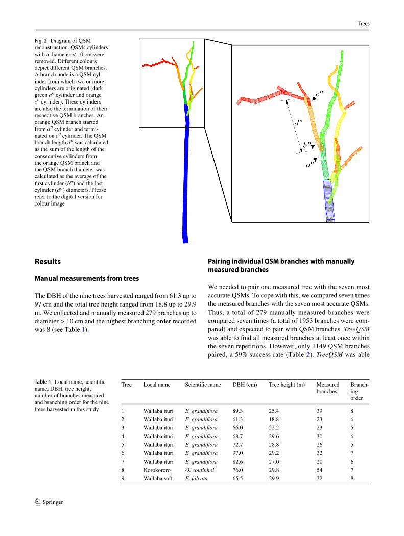
Finally, the geometrical structure and branching order from the QSMs were reconstructed following the meas-urements from the harvested trees (Fig. 2). A QSM branch node was defined as a QSM cylinder from which two or more cylinders are originated. This cylinder defined the termination of a QSM branch and the following cylinders are the origin of new QSM branches. Then, we defined a QSM branch as a collection of consecutive QSM cylinders which originate from a QSM branch node and terminates either:

• on another QSM branch node,• when a QSM cylinder reaches 10 cm diameter, or• when the QSM branch ends

The QSM branch length was estimated as the sum of the length of all cylinders belonging to the QSM branch and the QSM branch diameter was estimated as the average of the first and last cylinder belonging to the QSM branch.

Visual branch‑by‑branch pairing

The manually measured tree and QSM tree were visually paired branch-by-branch. The architecture of the manually measured tree was followed and each individual manually measured branch was located and identified. Then, we visually paired the measured branch with a QSM branch following the architecture of the QSM tree. Manually measured branches which did not have a QSM pair at all were excluded for further analysis. In the case that a manually measured branch was a suitable pair to two or more QSM branches, the similarity of each QSM branch with their manually measured counterpart was analysed. The length and diameter of each QSM branch were the parameters used to analyse quantitatively the similarity of branches. Because length and diameter had different orders of magnitude (one order of magnitude difference in length parameter is a hundred order of magnitude dif-ference in branch diameter), we could not compare them using Euclidian distance. To overcome this, a special type of Euclidian distance, the Diagonal-norm approach (Bezdek 1981) was applied. The diagonal-norm approach computed standardized values for both parameters and allowed us to compare them quantitatively in the same order of magnitude. Then, the QSM branch most similar to the manually measured branch in standardized length and standardized diameter was chosen as the best fitted pair.

Tree metrics assessment

We examined the absolute and relative error to evaluate branch length and diameter accuracy per individual paired branch. A confusion matrix was used to validate the accu-racy of our branching order method when compared to our manual measured dataset. Finally, the relative error was used to compare the cumulative length and the cumulative branch volume of total branches (as the aggregation of all paired branches) and separated by diameter classes. The cumulative branch length was calculated as the sum of branches’ length per cumulated diameter class. Likewise, the cumulative branch volume was calculated as the total sum of branches’ volume per cumulated diameter class. The length and mean diameter values of each branch were used to calculate branch volume.

Trees

1 3

Results

Manual measurements from trees

The DBH of the nine trees harvested ranged from 61.3 up to 97 cm and the total tree height ranged from 18.8 up to 29.9 m. We collected and manually measured 279 branches up to diameter > 10 cm and the highest branching order recorded was 8 (see Table 1).

Pairing individual QSM branches with manually measured branches

We needed to pair one measured tree with the seven most accurate QSMs. To cope with this, we compared seven times the measured branches with the seven most accurate QSMs. Thus, a total of 279 manually measured branches were compared seven times (a total of 1953 branches were com-pared) and expected to pair with QSM branches. TreeQSM was able to find all measured branches at least once within the seven repetitions. However, only 1149 QSM branches paired, a 59% success rate (Table 2). TreeQSM was able

Fig. 2 Diagram of QSM reconstruction. QSMs cylinders with a diameter < 10 cm were removed. Different colours depict different QSM branches. A branch node is a QSM cyl-inder from which two or more cylinders are originated (dark green a′′ cylinder and orange c′′ cylinder). These cylinders

are also the termination of their respective QSM branches. An orange QSM branch started from d′′ cylinder and termi-nated on c′′ cylinder. The QSM branch length d′′ was calculated as the sum of the length of the consecutive cylinders from the orange QSM branch and the QSM branch diameter was calculated as the average of the first cylinder ( b′′ ) and the last cylinder ( d′′ ) diameters. Please refer to the digital version for colour image

Table 1 Local name, scientific name, DBH, tree height, number of branches measured and branching order for the nine trees harvested in this study

Tree Local name Scientific name DBH (cm) Tree height (m) Measured branches

Branch-ing order

1 Wallaba ituri E. grandiflora 89.3 25.4 39 82 Wallaba ituri E. grandiflora 61.3 18.8 23 63 Wallaba ituri E. grandiflora 66.0 22.2 23 54 Wallaba ituri E. grandiflora 68.7 29.6 30 65 Wallaba ituri E. grandiflora 72.7 28.8 26 56 Wallaba ituri E. grandiflora 97.0 29.2 32 77 Wallaba ituri E. grandiflora 82.6 27.0 20 68 Korokororo O. coutinhoi 76.0 29.8 54 79 Wallaba soft E. falcata 65.5 29.9 32 8

Trees

1 3

to reconstruct more than 95% of the branches thicker than 30 cm. These branches were mostly the main stem and big branches. However, the reconstruction accuracy decreased for thinner branches (which usually have also lower point cloud density). TreeQSM reconstructed less than 56% of the branches with diameter measured between 10 and 30 cm.

Branch length from QSMs

We analysed the performance of TreeQSM by comparing the length of QSMs branches against the length of our manu-ally measured branches and calculating the absolute error difference between diameter classes (Table 3 and Fig. 3a). For average length values per classes, refer to Table OR4.1

in Online Resource 4. For branches greater than 50 cm diameter, the length of QSMs branches was overestimated by 1% (0.21 m larger on average than the manually meas-ured branches). TreeQSM had lower accuracy reconstruct-ing length for branches smaller than 50 cm diameter. The length of QSM branches was underestimated by 20% (0.58 m shorter on average) when compared to its measured counterpart.

Branch diameter from QSMs

For branches greater than 60 cm in diameter, the diameter of QSMs branches was underestimated by 6% (3.44 cm thinner on average than that of the measured branches) as seen in Table 3 and Fig. 3b. For average diameter values per classes, refer to Table OR4.1 in Online Resource 4. For branches with a diameter between 20 and 60 cm, TreeQSM underesti-mated the diameter by 8% ( 3.46 cm thinner on average than measured branches). Also TreeQSM did not perform well for branches between 10 and 20 cm. For these branches, QSMs diameters were overestimated by 40% (5.14 cm thicker on average).

Branching order from paired QSMs

The confusion matrix revealed that our method was very accurate in assigning the correct branching order when compared to the branching order of our manually measured paired dataset (Table OR5.1 in Online Resource 5). Our method correctly assigned 1143 QSM paired branches with an overall accuracy of 99% and an overall kappa coefficient of 0.99. Only 6 QSM branches were assigned incorrectly, and all of these were assigned to higher branching orders.

Absolute and cumulative branch length and branch volume from QSMs

The absolute length and absolute volume of TreeQSM matched branches were compared with the absolute length and absolute volume of manually measured matched branches by diameter classes (Table 4). When analysing by diameter classes, for branches between 10 and 20 cm, TreeQSM underestimated the absolute branch length by 30%. For thicker branches, with diameter between 20 and 50 cm, absolute branch length is underestimated by 17% and for branches thicker than 50 cm, is slightly overestimated by 1%. On the other hand, TreeQSM greatly overestimated the absolute branch volume for branches between 10 and 20cm (40%). However, for the branches with diameter between 20 and 50 cm, TreeQSM underestimated the absolute branch volume by 29%. For thicker branches (> 50 cm), the abso-lute volume is slightly underestimated by 0.4% (Table 4).

Table 2 Manually measured branches and the average and standard deviation of the most accurate QSM branches with TreeQSM (7 rep-etitions) by diameter classes

Accuracy shows the percentage of manually measured branches suc-cessfully reconstructed by TreeQSM. Our analysis was based only using QSM branches that could be paired with a manually measured branch

Diameter class (cm)

Measured branches

Average of QSM branches Accuracy (%)

10–20 160 72.29 ± 13.03 4520–30 67 44.86 ± 7.27 6730–40 26 21.86 ± 9.14 8440–50 11 10.14 ± 3.93 9250–60 7 7 ± 0.0 10060–70 5 5 ± 0.0 100≥ 70 3 3 ± 0.0 100

Table 3 Average absolute error and average relative error for QSM branches by diameter classes

Our analysis was based on the QSM branches which paired a manu-ally measured branch. Negative values indicated a model underesti-mation while positive values indicate a model overestimation com-pared to the manually measured branches

Diameter class (cm)

Absolute error ± SD Relative error

Length (m) Diameter (cm)

Length (%) Diameter (%)

10–20 – 1.03 ± 1.81

5.14 ± 5.5 12 40

20–30 – 0.67 ± 1.5 – 0.65 ± 4.76 10 – 230–40 – 0.42 ±

2.19– 5.33 ± 5.26 37 – 15

40–50 – 0.21 ± 1.37

– 4.23 ± 7.83 19 – 9

50–60 – 0.1 ± 0.76 – 3.61 ± 8.98 – 1 – 760–70 0.34 ± 0.4 – 5.33 ± 5.68 3 – 9≥ 70 0.39 ± 0.3 – 1.54 ± 0.8 2 – 2

Trees

1 3

The cumulative branch length and cumulative branch volume of each TreeQSM tree were compared to the same parameters of each manually measured tree (Table 5). When analysing all measured branches, TreeQSM under-estimated the length by 13%. TreeQSM only slightly overestimated below 1% the length of branches thicker than 40 cm compared to the manual measurements. When summing branches up to 20 cm diameter, the accuracy decreased and the cumulative length was underesti-mated by 6%. Similarly, TreeQSM tended to underesti-mate the cumulative volume when compared to manual

measurements (Table 5). When analysing all measured branches, TreeQSM underestimated the volume by 3%. For branches thicker than 50 cm, the volume of QSM branches was overestimated by 1% and the cumulative accuracy decreased when summing thinner branches. For branches thicker than 30 cm, TreeQSM underestimated volume by 3%.

Fig. 3 Absolute error for length for each unique QSM branch (a) and diameter (b). The solid black horizontal line depicts a perfect match (absolute error of 0 m). Vertical lines depict the range of values of

the seven reconstructions of the QSM per tree and the dot depicts the average value from the seven repetitions. Coefficient a denotes each tree main stem

Table 4 Absolute values for manually measured branches and absolute values and relative error for QSM branches for the absolute branch length and absolute branch volume separated by 10 cm diameter classes

Values shown are the average values and standard deviation from the seven models

Diameter class (cm)

Absolute branch length (m) Absolute branch volume (m3)

Measured branches QSM branches Relative error (%)

Measured branches QSM branches Relative error (%)

10–20 25.50 ± 8.21 17.82 ± 6.49 − 30 0.44 ± 0.15 0.61 ± 0.34 4020–30 13.51 ± 4.86 9.78 ± 4.62 − 28 0.66 ± 0.23 0.47 ± 0.24 − 2930–40 6.61 ± 5.49 5.61 ± 3.53 − 15 0.6 ± 0.45 0.42 ± 0.28 − 3040–50 4.16 ± 2.16 3.80 ± 1.6 − 8 0.66 ± 0.38 0.49 ± 0.22 − 2650–60 14.88 ± 6.77 14.88 ± 6.85 − 1 3.39 ± 1.74 3.62 ± 2.05 760–70 11.22 ± 7.65 11.56 ± 7.94 3 3.47 ± 2.38 3.28 ± 2.42 − 5≥ 70 21.23 ± 4.57 21.62 ± 4.79 2 9.51 ± 2.19 9.25 ± 2.02 − 3

Trees

1 3

Discussion

Our TLS and the TreeQSM method correctly identified and reconstructed 95% of the measured branches thicker than 30 cm diameter, 67% of the measured branches with diameter between 20 and 30 cm and 45% of the measured branches thinner than 20 cm diameter. Our method was exceptionally accurate assigning branching order (Fig. 4). However, we identified limitations with this method for reconstructing the length of measured branches less than 50 cm and the diameter of measured branches thinner than 20 cm. In a similar study on non-tropical trees, (Hack-enberg et al. 2015b) found that branches with diameter thicker than 10 cm were reconstructed accurately, but with smaller branches, especially twigs with diameter thinner than 4 cm, models overestimated branch volume. In a study by Kaasalainen et al. (2014) branches with diameter thinner than 5 cm were hardly visible in the point cloud and therefore were mostly left out of the model.

Our method underestimated absolute measured branch cumulative length on average by 13%. When analysing by cumulative diameter classes, our method slightly overes-timated less than 1% the length of cumulative measured branches thicker than 40 cm. When including thinner measured branches (up to 20 cm), the absolute measured length was underestimated by 6%. Dassot et al. (2012) found that reconstructed stem length agreed well with destructive measurements while reconstructed length of thinner branches did not.

Moreover, our method tended to slightly overestimate the length of thicker branches and underestimate the length of thinner branches (Table 4). This pattern was also observed in the relative error of the cumulated branches (Table 5). The relative error of the absolute branch length was greater as branches got thinner (Table 4). However, the cumulative branch length did not reflect this pattern, due to the small influence of the length of smaller branches

when compared to the absolute length of our measured branches.

Similarly, our method underestimated the absolute branch volume by 3%. When analysing by cumulated diameter classes, our method slightly underestimated the estimated volume of branches thicker than 50 cm by 1%. When including thinner branches (below 20 cm), cumula-tive branch volume underestimation increased up to 4%. This systematic underestimation of tree volume regard-less of species or absolute volume was also reported by Dassot et al. (2012); Gonzalez de Tanago et al. (2017); Calders et al. (2015). Similar studies also described sim-ilar accuracy values, Gonzalez de Tanago et al. (2017) showed an overall underestimation of 4% and Hackenberg et al. (2015a) described a absolute relative error of 8% compared to volume reference data. Although our method greatly underestimated the volume of thinner measured branches (Table 4), these did not contribute significantly to the cumulative branch volume, as seen in Table 5.

A conceptual difference where the main stem terminated was found between the manual measurements and the tree reconstruction. In the manual measurements, the length of the main stem stopped where the stem began to widen, before the point of furcation (Fig. 1); while in our method (Fig. 2), the length of the main stem terminated where the actual furcation was. The point of the manual measurement was up to several meters below where the measured branch split occurred and where the TreeQSM reconstructed a new branch. Thus, we took new measurements using the tree point cloud. The new measurements lowered the absolute error from 4.6 to 0.7 m. Based on our results, we recommend for future research to explicitly define a measured branch starting from the base of a branch. An ambiguous branch definition might lead to higher uncertainty in the length of the QSM branch. In addition, we observed that some big branches were destroyed during tree felling and could not be manually measured afterwards. Luckily, these branches

Table 5 Cumulative values and relative error (%) for cumulative branch length and branch volume for manual measurements and TreeQSM models

Negative values show underestimation while positive values show overestimation. Values are average val-ues from the seven models

Cumulative branch length (m) Cumulative branch volume (m3)

Cum. branch diameter (cm)

Measured branches

QSM branches Relative error (%)

Measured branches

QSM branches Relative error (%)

≥ 70 21.23 21.62 2 9.51 9.25 − 3≥ 60 32.45 33.18 2 12.98 12.52 − 3≥ 50 47.33 47.92 1 16.36 16.15 − 1≥ 40 51.49 51.71 0.4 17.02 16.64 − 2≥ 30 58.10 57.33 – 1 17.63 17.05 − 3≥ 20 71.61 67.11 −6 18.29 17.52 − 4Measured tree 97.11 84.93 – 13 18.73 18.14 − 3

Trees

1 3

had been scanned before felling, and thus appeared in the point cloud and were reconstructed by TreeQSM. As such, in the future, we suggest that the destroyed branches should be taken into account during the reconstruction process, because a missing branch might confuse the branching order and misclassify the QSM branch.

While our tree reconstruction method helped us to under-stand the architecture of the branches, it also constrained representing the architectural complexity. In this study, we enforced a simple cylinder-fractal structure of trees and lost details of the complex nature of the architecture of trees. Figure 1 shows that branch daughters exactly originated from a single branch node. However, two branches might originate from different branches nodes which are very close to each other and they might be confused as one branch node. While in this study we did not find this case, future studies should take into account the exact point of furcation as the origin of the branches. Enforcing a cylindrical struc-ture also impacted the buttresses modelling. In this study, the presence of buttresses did not impact our branches analy-sis. Moreover, the TreeQSM version used for this analysis was not able to render buttresses, thus we assumed them as cylinders. Recent work done by Gonzalez de Tanago et al. (2017) suggested that the modelling of buttresses has an impact on decreasing uncertainty on total tree volume and encouraged further studies to analyse buttresses in depth. In addition, we applied a simplification algorithm to reduce the number of output cylinders. This step reduced the number of cylinders by, either removing specific cylinders (based on our threshold), or merging two or three cylinders into a larger one. Nevertheless, this simplification indirectly added uncertainty in the reconstruction. Figure 2 shows three cyl-inders originating from the blue branch. While two cylin-ders originated from a very close furcation point, the first cylinder originated below this furcation point. However, the simplification process of our method created a single cylin-der and simplified the output model.

The quality of any TreeQSM output is a reflection of the quality of the point cloud on which it was based and the accuracy assessed for reconstruction. Several studies proved that TreeQSM was able to reconstruct smaller branches with

high accuracy when these branches had sufficient point den-sity for an proper reconstruction (Raumonen et al. 2013; Calders et al. 2015; Åkerblom et al. 2017). In our study, we scanned the trees in dense tropical environments, which made it difficult to scan properly the smaller branches inside the crown. The quality of the point cloud is directly influ-enced by several factors such as: the distance between the TLS scanner and the scanned tree, the scanning parameters and the environment surrounding the tree. The distance from the instrument to the tree canopy was especially noticed, which is the farthest path from the TLS scanner, surrounded by under story and (very often) lianas. The presence of lia-nas did not help us in the reconstruction process; however, in this study we are not modelling tree volume, and so the effects were not considered important. Even though our results showed that TreeQSM could not reconstruct thinner branches (it found 56% of branches between 10 and 30 cm diameter), the deviations of the TreeQSM matched branches from the real data measured in the field are relatively small. Moreover, we scanned with an angular resolution of 0.06◦ , which had proven to be a good trade-off between accuracy and time requirements for estimating other tree parameters (Calders et al. 2015; Gonzalez de Tanago et al. 2017; Wilkes et al. 2017), but might not be the most adequate parameter for inside canopy measurements. Wilkes et al. (2017) sug-gested that an angular resolution of 0.01◦ might be a better choice when scanning branches in high detail. By decreasing the angular resolution to 0.01◦ , we would be increasing the point density at larger distances, capturing more details of branches at higher heights. However, by increasing the angu-lar resolution, we are also exponentially increasing the time scanning. Moreover, we are also increasing the chance that we capture the branches being swayed by the wind, creating a ghosting effect in the point cloud (Wilkes et al. 2017).

Occlusion (the hiding of some structural elements by others) is a big issue for scanning in the tropics, thus to avoid occlusion and capture branches in detail within the canopy, the scanner should be located within a gap in the understory or in flexible positions. Implementing a radial sampling design with flexible locations around the tree could potentially produce a more evenly distributed point density

Fig. 4 (a) E. grandiflora tree point cloud, (b) TreeQSM with branches > 10cm diameter reconstructed from the tree point cloud. (c) QSM branches classified by length, (d) by branch diameter, and (e) by branching order. (f) QSM branches which were paired with manually measured branches. Please refer to the digital version for colour image

Trees

1 3

along the tree (Wilkes et al. 2017) and avoid occlusion by the surroundings. Our study employed 9 fixed position and only 4 flexible positions (set up arbitrarily within canopy gaps to capture the tree canopy) for TLS scanning per plot (Online Resource 1). We suggest that further studies should increase the number of flexible scan positions. The inclusion of more flexible scan positions might increase the point density at plot level. Moreover, when scanning, one should take into account wind, which swayed the medium to small branches and introduced noise in the point cloud. Seidel et al. (2012) have recommended to avoid wind with speed greater than 5 m/s.

Although our sample size is small and dominated by one tree species, our methodology can be applied to most tree species. We suggest that future research can apply our meth-odology on trees with different architecture and compare the accuracy. Equally important, one should be aware of the presence of non-hardwood components (leaves), branches from other trees and lianas. Tree architecture relies mostly on hardwood measurements and the presence of leaves, for-eign branches and lianas introduces uncertainty in the branch reconstruction at canopy level. Lianas are very difficult to distinguish within the canopy and manually removing them creates extra work. In this paper, we systematically deleted all cylinders with diameter less than 10 cm to remove lia-nas. Future research on branch architecture in the tropics should aim to incorporate new algorithms for leaves and lianas removal.

The branching order is a very sensitive parameter. TreeQSM will reconstruct foreign cylinders from a point cloud which has not been properly cleaned (with lianas or branches from other trees). The presence of these foreign branches will add several levels to the branching order, espe-cially if those foreign branches are attached to the main stem, changing the order drastically. Even though the branching order was highly accurate with our paired branches, some branches were misclassified in higher branching orders.

We excluded branches thinner than 10 cm from our analy-sis. The low point density (due to the scanner angular resolu-tion used in this paper), the plot design (Online Resource 1) and the high occlusion (due to lianas and the same branches) inside the crown made the reconstruction of branches within the crown unreliable. Moreover, our field data collected only measurements of branches > 10 cm. While removal of branches below 10 cm facilitated branch reconstruction in this study, it also reduces the applicability of this method for further studies. Despite that, it does not complete discard it; future research could adopt this methodology for smaller branches and still have comparable results.

Our paper relied on visual inspection in several steps of this paper (Sects. "Tree architecture reconstruction" and "Visual branch-by-branch pairing"). Even though visual inspection is subjective, it was done heuristically based on

the expertise of the authors. Other studies relied on other parameters to optimize TreeQSM, e.g., Gonzalez de Tanago et al. (2017) used the absolute volume to estimate an optimal d. We could not apply the same optimization method as in Gonzalez de Tanago et al. (2017), since their method was optimized upon estimating biomass and their sample size was bigger than ours. Future research should focus on an automated TreeQSM optimization method, as proposed by Calders et al. (2015).

Conclusions

Our study assessed the accuracy of using TLS and TreeQSM to reconstruct tree architecture parameters (branch length, branch diameter, branching order, absolute, and cumulative measured tree length and absolute and cumulative estimated tree volume) from tropical tree point clouds. Our method is able to reconstruct accurately big branches (> 40 cm diam-eter), while for smaller branches the accuracy decreased. A series of limitations were discussed which could improve the constraints encountered in this study and improved the modelling of smaller branches. We encourage future studies to optimize the plot and sampling design to obtain a more optimal point cloud density for branches inside the canopy and to take other factors into account while scanning, such as wind and disturbance from sampling activities (Wilkes et al. 2017). Even though our results perform worse at the tree level, our approach still represents a significant step forward into studies of tree architecture based on TLS and TreeQSM which could accelerate and improve our under-standing of tree architecture and how it may influence eco-logical (Kempes et al. 2011; Rosati et al. 2013) and meta-bolic processes (West 1999b; Bentley et al. 2013) or, in turn, be shaped by those processes.

Author contribution statement AL coordinated the entire study; AL, LPB, HB and MH conceived the idea and designed the methodology; AL collected the data; AL, LPB and HB analysed the data; AL, and LPB led the writing of the manuscript. HB, CM, AS, MH, PR, TJ and YM contrib-uted critically to the drafts. All authors gave final approval for publication.

Acknowledgements This research is part of CIFOR’s Global Com-parative Study on REDD+. The funding partners whose support is greatly appreciated include the Norwegian Agency for Development Cooperation (Norad), the Australian Department of Foreign Affairs and Trade (DFAT), the European Union (EU), the International Cli-mate Initiative (IKI) of the German Federal Ministry for the Environ-ment, Nature Conservation, Building and Nuclear Safety (BMUB), the CGIAR Research Program on Forests, Trees and Agroforestry (CRP-FTA) with financial support from the donors to the CGIAR Fund and

Trees

1 3

ERA-GAS NWO-3DforMod project 5160957540. LPB, AS and YM were supported by an ERC Advanced Investigator Award to YM (GEM-TRAITS, 321131) and NERC grant NE/P012337/1. We acknowledge the collaboration of Guyana Forestry Commission for their support: Pradeepa Bholanath, Carey Bhojedat, Hans Sukhdeo and their team who assisted us for logistics and during the tree harvesting in Guyana. The author thanks Cornelis Valk for his aid in the QSM visualization.

Compliance with ethical standards

Conflict of interest The authors declare that they have no conflict of interest.

Open Access This article is distributed under the terms of the Crea-tive Commons Attribution 4.0 International License (http://creat iveco mmons .org/licen ses/by/4.0/), which permits unrestricted use, distribu-tion, and reproduction in any medium, provided you give appropriate credit to the original author(s) and the source, provide a link to the Creative Commons license, and indicate if changes were made.

References

Åkerblom M (2017) Inversetampere/Treeqsm: Initial Release. 10.5281/zenodo.844626, URL: https ://zenod o.org/recor d/84462 6

Åkerblom M, Raumonen P, Mäkipää R, Kaasalainen M (2017) Automatic tree species recognition with quantitative structure models. Remote Sensing of Environment 191:1–12. https ://doi.org/10.1016/j.rse.2016.12.002

Bentley LP, Stegen JC, Savage VM, Smith DD, von Allmen EI, Sperry JS, Reich PB, Enquist BJ (2013) An empirical assessment of tree branching networks and implications for plant allometric scaling models. Ecology Letters 16(8):1069–1078. https ://doi.org/10.1111/ele.12127

Bezdek JC (1981) Pattern Recognition with Fuzzy Objective Func-tion Algorithms, vol 25. Springer, US, Boston, MA, https ://doi.org/10.1007/978-1-4757-0450-1

Bremer M, Rutzinger M, Wichmann V (2013) Derivation of tree skeletons and error assessment using LiDAR point cloud data of varying quality. ISPRS Journal of Photogrammetry and Remote Sensing 80:39–50. https ://doi.org/10.1016/j.isprs jprs.2013.03.003

Burt A, Disney M, Raumonen P, Armston J, Calders K, Lewis P (2013) Rapid characterisation of forest structure from TLS and 3D modelling. In: International Geoscience and Remote Sensing Symposium (IGARSS 2013), IEEE, 128.197.168.195[PDF], pp 3387–3390, 10.1109/IGARSS.2013.6723555

Calders K, Newnham GG, Burt A, Murphy S, Raumonen P, Herold M, Culvenor D, Avitabile V, Disney M, Armston J, Kaasalainen M (2015) Nondestructive estimates of above-ground biomass using terrestrial laser scanning. Methods in Ecology and Evolution 6(2):198–208. https ://doi.org/10.1111/2041-210X.12301

Chéné Y, Rousseau D, Lucidarme P, Bertheloot J, Caffier V, Morel P, Belin É, Chapeau-Blondeau F (2012) On the use of depth camera for 3D phenotyping of entire plants. Computers and Electron-ics in Agriculture 82:122–127. https ://doi.org/10.1016/j.compa g.2011.12.007

Dassot M, Barbacci A, Colin A, Fournier M, Constant T (2010) Tree architecture and biomass assessment from terrestrial LiDAR measurements: a case study for some Beech trees (Fagus Syl-vatica). Silvilaser, Full proceedings

Dassot M, Colin A, Santenoise P, Fournier M, Constant T (2012) Terrestrial laser scanning for measuring the solid wood vol-ume, including branches, of adult standing trees in the forest

environment. Computers and Electronics in Agriculture 89:86–93. https ://doi.org/10.1016/j.compa g.2012.08.005

Gaaliche B, Aachi-Mezghani M, Trad M, Costes E, Lauri PE, Mars M (2016) Shoot Architecture and Morphology of Different Branch Orders in Fig Tree ( Ficus carica L.). International Journal of Fruit Science 16(4):378–394. https ://doi.org/10.1080/15538 362.2015.11266 99

Gonzalez de Tanago J, Lau A, Bartholomeus H, Herold M, Avitabile V, Raumonen P, Martius C, Goodman RC, Disney M, Manuri S, Burt A, Calders K (2017) Estimation of above-ground bio-mass of large tropical trees with terrestrial LiDAR. Meth-ods in Ecology and Evolution 2017(July):1–12. https ://doi.org/10.1111/2041-210X.12904

Hackenberg J, Morhart C, Sheppard J, Spiecker H, Disney M (2014) Highly Accurate Tree Models Derived from Terrestrial Laser Scan Data: A Method Description. Forests 5(5):1069–1105. https ://doi.org/10.3390/f5051 069

Hackenberg J, Spiecker H, Calders K, Disney M, Raumonen P (2015a) SimpleTree An Efficient Open Source Tool to Build Tree Mod-els from TLS Clouds. Forests 6(12):4245–4294. https ://doi.org/10.3390/f6114 245

Hackenberg J, Wassenberg M, Spiecker H, Sun D (2015b) Non Destructive Method for Biomass Prediction Combining TLS Derived Tree Volume and Wood Density. Forests 6(4):1274–1300. https ://doi.org/10.3390/f6041 274

Hallé F, Oldeman R (1970) Essai sur l’architecture et la dynamique de croissance des arbres tropicaux. Monographie de Botanique et de Biologie Végétale, {M}asson

Hallé F, Oldeman RAA, Tomlinson PB (1978) Tropical Trees and For-ests. Springer, Berlin Heidelberg, Berlin, Heidelberg, https ://doi.org/10.1007/978-3-642-81190 -6

Henning JG, Radtke PJ (2006) Detailed stem measurements of stand-ing trees from ground-based scanning lidar. Forest Science 52(1):67–80

Holopainen M, Vastaranta M, Kankare V (2011) Biomass estimation of individual trees using stem and crown diameter TLS measure-ments. International Archives of Photogrammetry, Remote Sens-ing and Spatial Information Sciences XXXVIII(August):29–31

Kaasalainen S, Krooks A, Liski J, Raumonen P, Kaartinen H, Kaasalainen M, Puttonen E, Anttila K, Mäkipää R (2014) Change detection of tree biomass with terrestrial laser scanning and quan-titative structure modelling. Remote Sensing 6:3906–3922. https ://doi.org/10.3390/rs605 3906

Kempes CP, West GB, Crowell K, Girvan M (2011) Predicting maxi-mum tree heights and other traits from allometric scaling and resource limitations. PLoS ONE 6(6): https ://doi.org/10.1371/journ al.pone.00205 51

Krooks A, Kaasalainen S, Kankare V, Joensuu M, Raumonen P, Kaasalainen M (2014) Tree structure vs. height from terrestrial laser scanning and quantitative structure models. Silva Fennica 48(2):1–11, 10.14214/sf.1125

Miller RB, Détienne P (2001) Major Timber Trees of Guyana. Wood Anatomy, volume 20 edn. Tropenbos series, Tropenbos Interna-tional, Wageningen, the Netherlands

Momo Takoudjou S, Ploton P, Sonké B, Hackenberg J, Griffon S, de Coligny F, Kamdem NG, Libalah M, Mofack GI, Le Moguédec G, Pélissier R, Barbier N (2017) Using terrestrial laser scanning data to estimate large tropical trees biomass and calibrate allomet-ric models: A comparison with traditional destructive approach. Methods in Ecology and Evolution 38(1):42–49. URL https://doi.org/10.1111/2041-210X.12933, 0608246v3

Muñoz G, Grieser J (2006) Climwat 2.0 for CROPWAT Pfeifer N, Gorte BH, Winterhalder D (2004) Automatic reconstruction

of single trees from terrestrial laser scanner data. International Archives of Photogrammetry, Remote Sensing and Spatial Infor-mation Sciences, p 35

Trees

1 3

Pueschel P, Newnham GG, Rock G, Udelhoven T, Werner W, Hill J (2013) The influence of scan mode and circle fitting on tree stem detection, stem diameter and volume extraction from terrestrial laser scans. ISPRS Journal of Photogrammetry and Remote Sens-ing 77:44–56. https ://doi.org/10.1016/j.isprs jprs.2012.12.001

Raumonen P, Kaasalainen M, Åkerblom M, Kaasalainen S, Kaartinen H, Vastaranta M, Holopainen M, Disney M, Lewis P (2013) Fast Automatic Precision Tree Models from Terrestrial Laser Scan-ner Data. Remote Sensing 5(2):491–520. https ://doi.org/10.3390/rs502 0491

Reinhardt D, Kuhlemeier C (2002) Plant architecture. EMBO reports 3(9):846–51. https ://doi.org/10.1093/embo-repor ts/kvf17 7

Rosati A, Paoletti A, Caporali S, Perri E (2013) The role of tree archi-tecture in super high density olive orchards. Scientia Horticulturae 161:24–29. https ://doi.org/10.1016/j.scien ta.2013.06.044

Rosell J, Lloyd J, Sanz R, Arnó J, Ribes-Dasi M, Masip J, Escolà A, Camp F, Solanelles F, Gràcia F, Gil E, Val L, Planas S, Palacín J (2009) Obtaining the three-dimensional structure of tree orchards from remote 2D terrestrial LIDAR scanning. Agricultural and For-est Meteorology 149(9):1505–1515. https ://doi.org/10.1016/j.agrfo rmet.2009.04.008

Seidel D, Fleck S, Leuschner C (2012) Analyzing forest canopies with ground-based laser scanning: A comparison with hemispherical photography. Agricultural and Forest Meteorology 154–155:1–8. https ://doi.org/10.1016/j.agrfo rmet.2011.10.006

Thies M, Pfeifer N, Winterhalder D, Gorte BH (2004) Three-dimen-sional reconstruction of stems for assessment of taper, sweep

and lean based on laser scanning of standing trees. Scandina-vian Journal of Forest Research 19(6):571–581. https ://doi.org/10.1080/02827 58041 00195 62

Van der Zande D, Hoet W, Jonckheere I, van Aardt J, Coppin P (2006) Influence of measurement set-up of ground-based LiDAR for derivation of tree structure. Agricultural and Forest Mete-orology 141(2–4):147–160. https ://doi.org/10.1016/j.agrfo rmet.2006.09.007

West GB (1999a) The Fourth Dimension of Life: Fractal Geometry and Allometric Scaling of Organisms. Science 284(5420):1677–1679. https ://doi.org/10.1126/scien ce.284.5420.1677

West GB (1999b) The origin of universal scaling laws in biology. Phys-ica A: Statistical Mechanics and its Applications 263(1–4):104–113. https ://doi.org/10.1016/S0378 -4371(98)00639 -6

West GB, Brown JH, Enquist BJ (1997) A General Model for the Origin of Allometric Scaling Laws in Biology. Science 276(5309):122–126. https ://doi.org/10.1126/scien ce.276.5309.122

West GB, Enquist BJ, Brown JH (2009) A general quantitative theory of forest structure and dynamics. Proceedings of the National Academy of Sciences of the United States of America 106:7040–7045. https ://doi.org/10.1073/pnas.08122 94106

Wilkes P, Lau A, Disney M, Calders K, Burt A, Gonzalez de Tanago J, Bartholomeus H, Brede B, Herold M (2017) Data acquisition con-siderations for Terrestrial Laser Scanning of forest plots. Remote Sensing of Environment 196:140–153. https ://doi.org/10.1016/j.rse.2017.04.030