Quantifying ecological memory in plant and …...IDEA AND PERSPECTIVE Quantifying ecological memory in plant and ecosystem processes Kiona Ogle,1* Jarrett J. Barber,2 Greg A. Barron-Gafford,3

IDEA AND

PERSPECT IVE Quantifying ecological memory in plant and ecosystem

processes

Kiona Ogle,1* Jarrett J. Barber,2

Greg A. Barron-Gafford,3

Lisa Patrick Bentley,4

Jessica M. Young,5

Travis E. Huxman,6

Michael E. Loik7 and

David T. Tissue8

Abstract

The role of time in ecology has a long history of investigation, but ecologists have largelyrestricted their attention to the influence of concurrent abiotic conditions on rates and magnitudesof important ecological processes. Recently, however, ecologists have improved their understand-ing of ecological processes by explicitly considering the effects of antecedent conditions. Tobroadly help in studying the role of time, we evaluate the length, temporal pattern, and strengthof memory with respect to the influence of antecedent conditions on current ecological dynamics.We developed the stochastic antecedent modelling (SAM) framework as a flexible analyticapproach for evaluating exogenous and endogenous process components of memory in a systemof interest. We designed SAM to be useful in revealing novel insights promoting further study,illustrated in four examples with different degrees of complexity and varying time scales: stomatalconductance, soil respiration, ecosystem productivity, and tree growth. Models with antecedenteffects explained an additional 18–28% of response variation compared to models without ante-cedent effects. Moreover, SAM also enabled identification of potential mechanisms that underliecomponents of memory, thus revealing temporal properties that are not apparent from traditionaltreatments of ecological time-series data and facilitating new hypothesis generation and additionalresearch.

Keywords

Antecedent conditions, hierarchical Bayesian model, lag effects, legacy effects, net primary pro-duction, soil respiration, stomatal conductance, time-series, tree growth, tree rings.

Ecology Letters (2015) 18: 221–235

INTRODUCTION

Temporal phenomena are fundamental to ecology. Thegrowth patterns encoded in tree rings, the timing of floweringand production within a season, and the scheduling of repro-duction within an organism’s lifespan are examples from earlyattempts to understand the role of time in ecology. Studies ofecological succession in the early 1900s provide a process-based interpretation of mechanisms underlying some ecologi-cal patterns over time and of the importance of antecedentevents (Johnson & Miyanishi 2008). More recently, the timingof migration, flowering, and pollination has taken on criticalimportance given the potential for differences in activitybetween mutualistic partners within a rapidly changing cli-mate (Visser & Both 2005; Elzinga et al. 2007). Assumingconsistent relationships between space and time for evaluatingecological phenomena has been useful for tackling scientific

challenges in ecology (Levin 1992), but ecological patternsand processes are rarely static (Chave 2013), thus challengingour approaches for addressing the importance of time in ourscience.Despite the long history of studying the role of time in ecol-

ogy, we still lack a solid understanding of the temporal link-ages between abiotic events and biotic responses, theirinteractions, and feedbacks to the environment (e.g. Bardgettet al. 2005; Crooks 2005; Resco et al. 2009). For example,how do different abiotic events interact over time to drive eco-logical phenomena? How do ecological patterns and processesrespond to perturbations at different time scales? Abioticresources (e.g. water, nutrients) often are available to organ-isms in ephemeral pulses, and changes in their timing, dura-tion, and magnitude can lead to significant changes inecological structure and function (Schwinning & Sala 2004).For example, the effects of multiple precipitation events may

1School of Life Sciences, Arizona State University, Tempe, AZ, USA2School of Mathematical and Statistical Sciences, Arizona State University,

Tempe, AZ, USA3School of Geography and Development & B2 Earthscience, University of

Arizona, Tucson, AZ, USA4Environmental Change Institute, Oxford University Centre for the Environ-

ment, University of Oxford, Oxford, UK5International Arctic Research Center, University of Alaska, Fairbanks, AK,

USA

6Ecology and Evolutionary Biology & Center for Environmental Biology,

University of California, Irvine, CA, USA7Department of Environmental Studies, University of California, Santa Cruz,

CA, USA8Hawkesbury Institute for the Environment, University of Western Sydney,

Richmond, NSW, Australia

*Correspondence: E-mail: [email protected]

© 2014 John Wiley & Sons Ltd/CNRS

Ecology Letters, (2015) 18: 221–235 doi: 10.1111/ele.12399

be additive when the interval between pulses is short, but thiseffect decreases as the number of between-event dry daysincreases (Loik et al. 2004). In addition, after an extended dryperiod, the impact of a first pulse may or may not have conse-quences for the impact of subsequent events; however, werequire better knowledge about the mechanisms relatingecological responses to rainfall timing to generate generalprinciples.Although precipitation, temperature, and other factors

affect plant and ecosystem processes at multiple time scales,many analyses tend to assume, at least implicitly, that envi-ronmental conditions impact biological processes concur-rently. Ecological disturbances, however, are frequentlydescribed in terms of time-since-disturbance (e.g. fire, flood,frost, or storm damage). Presumably, we could gain a greaterunderstanding of the timing of many abiotic–biotic relation-ships with careful consideration of how past perturbations(resource pulses, disturbance, or environmental events) at dif-ferent scales modify the response of biological processes to arecent event. For example, in semi-arid systems, antecedenttemperature and water availability, averaged over several daysor weeks, may be more important than current conditions forplant, soil, and ecosystem carbon exchange (Ogle & Reynolds2002; Cable et al. 2008; Shim et al. 2009). Precipitation andtemperature patterns of past months, seasons, or years canalso impact soil respiration (Janssens et al. 2001; Fierer et al.2006; Vargas et al. 2011), leaf-level gas exchange (Patricket al. 2009), annual tree growth (i.e. ring widths, Fritts 1966;Graumlich 1991; Gagen et al. 2004), and ecosystem productiv-ity (Leuning et al. 2005; Coops et al. 2007; Sala et al. 2012;Reichmann et al. 2013).Despite their importance, we lack analytical frameworks for

quantifying antecedent conditions and their effects on currentprocesses, thus lending insight into ecological memory. Tradi-tional schemes to evaluate ecological time-series data for driv-ers of current phenomena are often constrained by short-termexperimentation, space-for-time substitutions, or arbitrary des-ignations of the relative importance of past conditions thatcan introduce researcher bias. Here, we improve our capacityto evaluate the role of the past by developing an analyticalframework for simultaneously quantifying the length, tempo-ral patterns, and strength of ecological memory. Such aframework is expected to elicit new experiments to test under-lying mechanisms and to improve forecasts of ecologicalresponses to future environmental change by better contextu-alising the role of time.

ECOLOGICAL MEMORY

Ecological memory has been defined as ‘the capacity of paststates or experiences to influence present or future responsesof the community’ (Padisak 1992), and as ‘the degree to whichan ecological process is shaped by its past modifications of alandscape’ (Peterson 2002). Our definition of memory alignswith these definitions, but we explicitly consider three primarycomponents: (1) the length of the memory, which quantifiesthe time period(s) over which antecedent conditions or statesaffect current processes or states, (2) the temporal pattern ofthe memory, which is characterised by variation in the relative

importance of conditions occurring at different times into thepast, including potentially important time lags and (3) thestrength of the memory, which describes the degree to whichantecedent conditions affect the process of interest.Furthermore, we find it convenient to distinguish between

exogenous and endogenous memory (Bengtsson et al. 2003;Lundberg & Moberg 2003; Golinski et al. 2008; Schaefer 2009;Barron-Gafford et al. 2014). Here, we use exogenous memoryto refer to the effects of past external factors (typically environ-mental or abiotic) on the state of the system, as illustrated byimpacts of winter freeze–thaw dynamics on subsequent ecosys-tem production (Kreyling et al. 2010). We use endogenousmemory to refer to how past states of the system of interestinfluence current states of the same system, as in density depen-dent population growth where the current population growthrate and/or size depends are past population size (Golinskiet al. 2008). For ecosystem-level processes (e.g. soil organicmatter decomposition), the endogenous effects could reflect theinfluence of past decomposition patterns or other, often biolog-ically mediated, ecosystem feedbacks (e.g. past litter fall rates,or past microbial biomass or activity). Endogenous effects,however, are infrequently explored in plant physiological andecosystem ecology, which tend to emphasise exogenous factors,but quantification of endogenous memory may lend insightinto potentially important biological feedbacks.Our goal was to evaluate the length, temporal patterns, and

strength of memory in plant and ecosystem processes, and todesign a flexible quantitative framework that will enable us todo so with different conceptualisations of important biologicaldynamics. The framework should provide results that areeasily interpretable to ecologists while retaining general appli-

(a) (b)

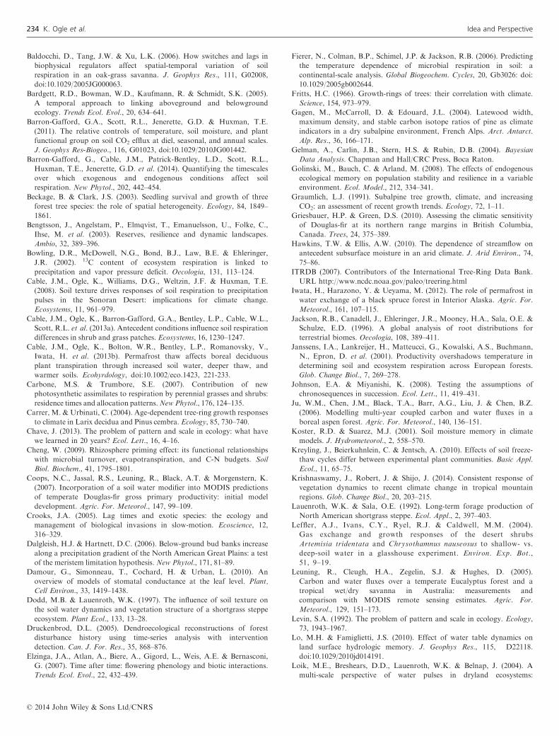
Figure 1 (a) Four hypothetical weight functions for continuous time. The

weight function indicated by w1 has a short memory length (L) such that

conditions beyond L = ta units into the past do not affect the current

process. Moreover, w1 takes on its highest value at j = 0, thus, current

conditions are most important. The weight function given by w2 has a

long memory (L ≤ te), and current conditions are still most important.

The weight function given by w3 has a medium-length memory (L ≤ td)

and a lag (conditions experienced at j = tb are most important). And w4

indicates that current conditions are most important, but a minor lag

occurs around j = tc. (b) Discretised weights associated with weight

function w3 (red bars); the discretised weights w3(j) multiply X(t�j) to

determine Xant as illustrated in Box 1.


222 K. Ogle et al. Idea and Perspective

cability. Here, we present a stochastic antecedent modelling(SAM) framework and apply it to four different case studiesto illustrate how the framework can be used to reveal memorycharacteristics for processes spanning a range of time scalesand system complexities: stomatal conductance, soil respira-tion, ecosystem annual net primary production, and annualtree growth. We use these examples to highlight issues sur-rounding five primary questions: (1) Does memory matter? (2)What are the temporal characteristics of memory? (3) Whattime scales are important for quantifying memory? (4) What

features underlie memory? (5) What mechanisms govern mem-ory? We end with a discussion about potential considerationsand extensions of the SAM framework beyond the illustrativeexamples provided in the current treatment.

THE STOCHASTIC ANTECEDENT MODELLING

FRAMEWORK

Let Y(t) represent an observed value of an ecological responseof interest (e.g. population size, photosynthetic rate, plant bio-

Box 1 Description of the general SAM approach

Each node indicates a quantity in the model, and the directed edges connecting nodes indicate conditional relationships (e.g.Xant depends on X and wX). The quantities can generally be classified as (1) stochastic data (e.g. the response of interest, Y), (2)fixed data (e.g. the observed covariates, X, Z and E), (3) latent or unknown processes such as the predicted response (l) andthe antecedent exogenous (Xant) and endogenous (Eant) covariates, (4) data parameters (e.g. r) describing observation uncer-tainty and (5) process parameters (e.g. a) giving rise to the latent processes.

Example data model: For observation or time t, and for some potential transformation of Y, g(Y), including g(Y) = Y, we mightassume:

g YðtÞð Þ�Normal lðtÞ; rð ÞNote that we are not restricted to the normal distribution.

Example process model for l: The model for l has the general form:

lðtÞ ¼ f XantðtÞ;EantðtÞ;ZðtÞ; að Þ þ et

Where f is a function to be determined on a case-by-case basis, and e represents additional sources of uncertainty (e.g. randomeffects that may be indexed by t or some other indexing variable, such as location, individual, etc.); for simplicity, we did notinclude e in the above graphical model. A vector of parameters (a) describes the effects of Xant, Eant and Z on the response ofinterest (Y or l).

Example process model for Xant and Eant: For time period j into the past (j = 0 = current time):

XantðtÞ ¼XTlag

j¼0

Xðt� jÞ � wXðjÞ EantðtÞ ¼XTlag

j¼0

Eðt� jÞ � wEðjÞ

Example priors: For the weight vectors (w) and element k in the a vector:

wXð1 : ðTlagþ 1ÞÞ;wEð1 : ðTlagþ 1ÞÞ�Dirichletð1; 1; . . .; 1Þ;ak �Normalð0;SÞ; r�Uniformð0;AÞ

Values of S and A are typically chosen to achieve relatively non-informative priors, and the normal and uniform priors couldbe exchanged for other distributions that may be more appropriate in particular cases.


Idea and Perspective Quantifying ecological memory 223

mass) measured at time t. We characterise the variability ofY(t) about its mean (or latent process), l(t), with a probabilitydistribution, which we refer to as the ‘data model’ (see Box 1).Next, we specify a model for l(t) (Box 1) that incorporatesthe effects of antecedent exogenous (Xant; e.g. antecedent soilwater, temperature, precipitation), antecedent endogenous[Eant; e.g. past values of Y or its latent value (l)] and currentconditions (Z). The effects of these variables on the currentprocess are captured by the process parameters (e.g. a, avector of effects parameters), and the magnitude and signifi-cance of the antecedent effects (components of a) characterisethe overall strength of memory.We define a stochastic model for each antecedent variable. A

simple model for Xant or Eant sums over past conditions,weighted by their relative importance (w) (Fig. 1; Box 1).Unlike previous approaches (e.g. Ogle & Reynolds 2002; Leu-ning et al. 2005; Fierer et al. 2006; Cable et al. 2008), we do notarbitrarily compute Xant or Eant by assuming fixed values for w(e.g. such as computing the average of the past values over anarbitrarily chosen time period). For each time step j into thepast, SAM allows data on Y to inform the unknown relativeimportance, w(j)’s, of past exogenous, X(t�j), or endogenous, E(t�j), variables for predicting the response at time t (Box 1). Animportant aspect of the model(s) for Xant and Eant is the specifi-cation of the time scales associated with computing the w(j)’s,including determining the number of past time periods to sumover (Tlag, Box 1), and the size of the time step j (e.g. every 6 h,daily, weekly, etc.). We describe potential strategies to address-ing these issues in Appendix S1.The temporal pattern of the memory is revealed by variation in

the w(j)’s, and comparably high values for particular w(j)’s indi-cate potential lag times (e.g. for daily time steps, a high value ofw(4) would indicate a 4-day lag). The length of the memorydescribes the length of time over which past conditions signifi-cantly influence the current process. For example, the memorylength (L) may be defined as the past time for which the cumula-tive weights achieve some specified threshold (c) that is ‘close’ toone, such that the solution for L satisfies

PLj¼0 wðjÞ ¼ c. For

example, for daily time steps, if L = 10 (say, for c = 0.90), thenthis indicates a memory of length 10 days such that conditionsoccurring more than 10 days ago do not appreciably (< 10%chance) affect the current process of interest.We implement SAM in a Bayesian framework because of its

ability to accommodate the stochastic data model, the stochas-tic antecedent model, the non-linear model for l that emergesby making Xant and/or Eant stochastic and required constraintson the w’s; we refer readers to Gelman et al. (2004) and Ogle& Barber (2008) for a more thorough description of the Bayes-ian approach. Our interpretation of the w’s as the relativeimportance of past conditions requires that each be between 0and 1 and that all sum to 1. Thus, in the Bayesian context, wechose an appropriate prior (e.g. Dirichlet distribution, Gelmanet al. 2004) that obeys these constraints (Box 1).

EVALUATING ECOLOGICAL MEMORY WITH THE SAM

FRAMEWORK

We present four case studies to illustrate our SAM frame-work. The first is based on annual aboveground net primary

productivity (ANPP, g m�2 year�1) of a shortgrass steppeecosystem in northern Colorado; ANPP data summaries (sam-ple means) were extracted from the literature (Lauenroth &Sala 1992). The second involves tree-ring widths (r, mm/year),an index of annual tree productivity, of Pinus edulis (pinyonpine) growing near Montrose, Colorado. The original r datawere downloaded from the International Tree-Ring DataBank (ITRDB 2007), and were contributed by Woodhouseet al. (2006). The third uses original data on soil respirationrates (Rs, lmol CO2 m�2 s�1) in two microhabitats (undershrubs vs. bunchgrasses) occurring in the Sonoran Desert nearTucson, Arizona (see Barron-Gafford et al. 2011, 2014). Thefourth focuses on leaf-level stomatal conductance (gs,mol H2O m�2 s�1) of a common desert shrub (Larrea triden-tata, creosotebush) growing in the Chihuahuan Desert insouthern New Mexico (see Ogle & Reynolds 2002).These case studies were chosen because they represent pro-

cesses operating at different biological, temporal, and/or spa-tial scales, as well as different complexities of endogenousand exogenous processes. The ANPP and r examples repre-sent relatively long time scales (yearly) and the Rs and gsexamples represent short time scales (instantaneous, sub-dailyrates). We use the ANPP case study to illustrate a simpleapplication of the SAM framework, and the associatedmodel code is provided in Appendix S2. The ANPP and rcase studies are used to demonstrate nested memory timescales, and the r example also allows us to evaluate memoryproperties at different levels of organisation (e.g. individualsvs. populations). The gs example illustrates how differentmemory components may operate at different, non-nestedtime scales (e.g. sub-daily to weekly). The Rs and r casestudies both provide an evaluation of endogenous and exoge-nous memory, and the Rs example also explicitly evaluatesthe effects of current and antecedent factors, and their inter-actions.Descriptions of the data and processes associated with each

case study and the associated components comprising theBayesian SAM framework are highlighted in Box 2. For theantecedent importance weights (w), it seems natural to us tochoose monthly and annual time steps for the annual produc-tivity variables (r and ANPP), and sub-hourly, hourly, and/ordaily time steps for the fast (sub-daily) time-scale variables (gsand Rs). The basic structure of the process model for l in thegs example is motivated by the model described in Ogle &Reynolds (2002), but we made significant modifications toinclude the antecedent variables and their effects. The modelfor Rs is described in detail in Barron-Gafford et al. (2014).The models developed for the ANPP and r case studies havenot been previously described, but were motivated by empiri-cal descriptions of the potential importance of past climateconditions (Fritts 1966; Graumlich 1991; Lauenroth & Sala1992; Druckenbrod 2005; Sherry et al. 2008). In each casestudy, we opted for relatively simple models that are easy tointerpret, motivated by the original publications, and thatcaptured a significant amount of variation in the response var-iable (e.g. Table 1). Other, potentially better models could beapplied, but a comprehensive examination of different modelsis beyond the scope of this study. Importantly, each casestudy and its associated SAM formulation offer unique attri-



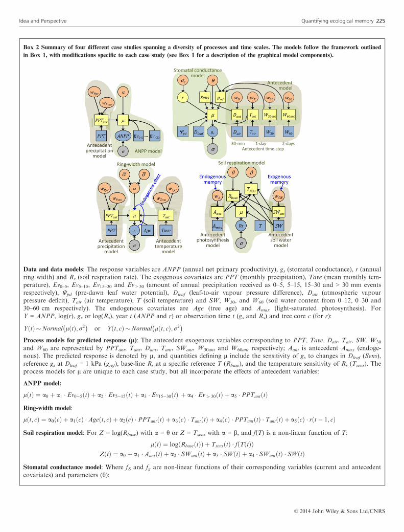
Box 2 Summary of four different case studies spanning a diversity of processes and time scales. The models follow the framework outlined

in Box 1, with modifications specific to each case study (see Box 1 for a description of the graphical model components).

Data and data models: The response variables are ANPP (annual net primary productivity), gs (stomatal conductance), r (annualring width) and Rs (soil respiration rate). The exogenous covariates are PPT (monthly precipitation), Tave (mean monthly tem-perature), Ev0–5, Ev5–15, Ev15–30 and Ev>30 (amount of annual precipitation received as 0–5, 5–15, 15–30 and > 30 mm eventsrespectively), Ψpd (pre-dawn leaf water potential), Dleaf (leaf-to-air vapour pressure difference), Dair (atmospheric vapourpressure deficit), Tair (air temperature), T (soil temperature) and SW, W30, and W60 (soil water content from 0–12, 0–30 and30–60 cm respectively). The endogenous covariates are Age (tree age) and Amax (light-saturated photosynthesis). ForY = ANPP, log(r), gs or log(Rs), year t (ANPP and r) or observation time t (gs and Rs) and tree core c (for r):

YðtÞ�Normal lðtÞ; r2� �or Yðt; cÞ�Normal lðt; cÞ; r2� �

Process models for predicted response (l): The antecedent exogenous variables corresponding to PPT, Tave, Dair, Tair, SW, W30

and W60 are represented by PPTant, Tant, Dant, Tant, SWant, W30ant and W60ant respectively; Aant is antecedent Amax (endoge-nous). The predicted response is denoted by l, and quantities defining l include the sensitivity of gs to changes in Dleaf (Sens),reference gs at Dleaf = 1 kPa (gref), base-line Rs at a specific reference T (Rbase), and the temperature sensitivity of Rs (Tsens). Theprocess models for l are unique to each case study, but all incorporate the effects of antecedent variables:

ANPP model:

lðtÞ ¼ a0 þ a1 � Ev0�5ðtÞ þ a2 � Ev5�15ðtÞ þ a3 � Ev15�30ðtÞ þ a4 � Ev[ 30ðtÞ þ a5 � PPTantðtÞRing-width model:

lðt; cÞ ¼ a0ðcÞ þ a1ðcÞ � Ageðt; cÞ þ a2ðcÞ � PPTantðtÞ þ a3ðcÞ � TantðtÞ þ a4ðcÞ � PPTantðtÞ � TantðtÞ þ a5ðcÞ � rðt� 1; cÞSoil respiration model: For Z = log(Rbase) with a = h or Z = Tsens with a = b, and f(T) is a non-linear function of T:

lðtÞ ¼ log RbaseðtÞð Þ þ TsensðtÞ � fðTðtÞÞZðtÞ ¼ a0 þ a1 � AantðtÞ þ a2 � SWantðtÞ þ a3 � SWðtÞ þ a4 � SWantðtÞ � SWðtÞ

Stomatal conductance model: Where fS and fg are non-linear functions of their corresponding variables (current and antecedentcovariates) and parameters (h):



butes that allow us to address the five aforementioned ques-tions about ecological memory (see Ecological Memory sec-tion).

Does memory matter?

If memory matters, then SAM’s stochastic antecedent effectswill improve our ability to predict the response variable ofinterest. We compared a model with antecedent effects (SAMapproach) to a reduced model without antecedent effects;both models retain current exogenous or endogenous vari-ables. In each case study, the SAM approach resulted in supe-rior model fit (Table 1). The reduced model explained 46–47% (for gs, ANPP, and r) to 70% (for Rs) of the variation inthe observed data, whereas the SAM explained 70–75% (forgs, ANPP, and r) to 88% (for Rs) of the variation. In addi-tion, we computed the deviance information criterion (DIC,Spiegelhalter et al. 2002), a model comparison index thataccounts for model fit while penalising model complexity.Although SAM led to greater model complexity (with the

exception of Rs), in all four case studies, it notably improvedfit relative to the simple models as indicated by lower DICvalues (Table 1). This aligns with others studies that have alsoshown improvement in model fits when including antecedentvariables (e.g. Oesterheld et al. 2001; Leuning et al. 2005;Hawkins & Ellis 2010; Sala et al. 2012; Cable et al. 2013a;Barron-Gafford et al. 2014). The improved model perfor-mance yielded by SAM, however, is also accompanied bydetails on the characteristics of memory (i.e. length, temporalpatterns and strength).The strength of the memory response is quantified by the

magnitude and significance of the Xant and Eant effects param-eters (i.e. subcomponents of a in Box 1 and Box 2). In allfour case studies, at least one or more of the antecedent driv-ers was statistically significant such that the 95% credibleinterval (CI) for its corresponding a term did not contain zero(Table S1). For example, PPTant had a significant positiveeffect on ANPP (Table S1 or Fig. 2). In the original study,Lauenroth & Sala (1992) did not directly evaluate the impor-tance of antecedent precipitation, but they hypothesised that

lðtÞ ¼ grefðtÞ þ SensðtÞ �DleafðtÞSensðtÞ ¼ fS WpdðtÞ;DantðtÞ;TantðtÞ; h

� �grefðtÞ ¼ fg WpdðtÞ;TantðtÞ;W30antðtÞ;W60antðtÞ; h

� �

Process models for antecedent variables: The antecedent variables are defined similarly in all four examples, though, the timescale over which each is computed may differ:

Climate variables (for ANPP and r): For X = PPT or Tave (P or T subscript on w), Xant = PPTant or Tant, year y into the past,and month m:

XantðtÞ ¼X4

y¼0

X12

m¼1

Xðt� y;mÞ � wX;moðmjyÞ � wX;yrðyÞ

wX,mo(m|y) is the relative importance of X occurring in month m conditional on year y.

Other variables (for gs and Rs): For X = Amax, Dair, Tair, SW, W30 or W60 (with related subscripting for w), Xant = Aant, Dant,Tant, SWant, W30ant or W60ant, and time period j into the past:

XantðtÞ ¼XTlag

j¼s

Xðt� jÞ � wXðjÞ

s = 1 for SW for Rs such that current SW is not included in SWant since it explicitly occurs in the l model for Rs; s = 0 for allother variables. Tlag=5 days for Aant and SWant, 7 days for Tant and W30ant, 7 two-day blocks for W60ant and 6 half-hour blocksfor Dant.

Parameters and prior models: Variability in the observation errors is described by r; a is a vector of coefficients describing theeffects of the exogenous and endogenous covariates on l, where the core-level a’s in the r example vary around overall (mean)effects (�a), and �r describes variability among cores. Similarly, h and b are vectors describing the effects of the covariates on thelatent components giving rise to l. The w’s are the weights describing the relative importance of the different antecedent covari-ates occurring at different times into the past. The prior models are similar across all four examples. Let k denote an element ofeach a, �a , �r, h, and b vector, then:

wmo 1 : 12jyð Þ;wyr 1 : 5ð Þ;wX 1 : ðTlagþ 1� sÞð Þ�Dirichletð1Þ; akðcÞ�Normal �ak; �rkð Þðfor r modelÞor ak �Normalð0;SÞ; �ak; hk; bk �Normalð0;SÞ; and r; �rk �Uð0;AÞ

Where 1 is a vector of ones whose length (12, 5 or Tlag+1- s) is consistent with its corresponding w. ‘Large’ values of S and Awere chosen for fairly non-informative priors; semi-informative priors were used for a subset of h’s and b’s in the Rs model (seeBarron-Gafford et al. 2014 for details).

Box 2 (Continued)



ANPP exhibited time lags of several years in response to pastprecipitation patterns, and reanalysis of this data found thatthe current and previous year’s precipitation explained a sig-nificant amount of variation in ANPP (Oesterheld et al.2001). In the tree-ring example, r was significantly correlatedwith PPTant, Tant, and the previous year’s ring width, r(t–1, c)(Table S1). Higher precipitation in the past is expected to leadto greater growth in the current time period. The positive cor-relation between r(t,c) and r(t�1,c) is consistent with an auto-regressive, AR(1), process, which is commonly used in

dendrochronological analyses (Monserud & Marshall 2001;Griesbauer & Green 2010; Tingley et al. 2012), but whichlacks the memory interpretations of the SAM approach.

What are the temporal characteristics of memory?

Having determined that antecedent effects are significant, weproceed to evaluate the length and temporal patterns of thememory response. If an antecedent effect is not significantlydifferent from zero (i.e. it has weak memory or no memory),then its corresponding w’s are meaningless. In all four casestudies, the posteriors for the w’s differed from the priors inmeaningful ways. In the ANPP case study, the posterior forwP,yr (annual precipitation weights) was tighter than the prior,as reflected by comparatively narrow posterior 95% CIs(Fig. 2), and unlike the ‘flat’ prior, the posterior exhibitednotable temporal patterns. For example, precipitation received1–2 years ago was significantly more important than thatreceived during the year of production or 4 years ago (i.e. the95% CIs for wP,yr(1) and wP,yr(2) do not contain the posteriormeans for wP,yr(0) and wP,yr(4), and vice versa). The moder-ately low value for the current year’s precipitation weight wasnot surprising since it sums over a subset of months thatoccurred after the ANPP harvests (i.e. wP,mo = 0 for thesemonths). Differences between the prior and posterior w’s wereeven more obvious for gs (Fig. 3) and r (Fig. 4); the posteriorCI widths were notably narrower than the prior CI widths,and a subset of w’s – e.g. the importance of deep soil water(W60) experienced 7–8 weeks ago (w60, j = 5; Fig. 3), and sev-eral wP,mo’s associated with PPTant weights in the r model(Fig. 4) – are associated with posterior estimates that are sig-nificantly different from the prior.Temporal patterns in the weights also revealed important

time lags. For example, gs exhibited a short lag with respectto shallow soil water (W30), temperature (Tair) and vapourpressure deficit (Dair) such that conditions occurring the dayprior to, the day of, or half-an-hour prior to the observed gs,respectively, were most important for predicting gs (Fig. 3b–d). Yesterday’s soil water conditions were also most important

Table 1 Summary of model comparison indices for the four case studies

in Box 2: stomatal conductance (gs), annual aboveground net primary

productivity (ANPP), soil respiration (Rs) and tree-ring widths (r)

Example Model R2 DIC Dbar pD

gs Reduced 0.46 �4735.0 �4764.0 28.7

SAM 0.72 �5240.0 �5334.0 93.9

Difference 0.26 �505.0 �570.0 65.2

ANPP Reduced 0.47 454.1 446.6 7.6

SAM 0.75 435.4 420.2 15.2

Difference 0.28 �18.7 �26.4 7.6

Rs Reduced 0.70 323.5 297.2 26.3

SAM 0.88 187.5 164.5 22.9

Difference 0.18 �136.0 �132.7 �3.4

r Reduced 0.47 �2422.0 �2488.0 65.6

SAM 0.70 �3413.0 �3518.0 105.1

Difference 0.23 �991.0 �1030.0 39.5

Model fit is evaluated via the R2 value obtained by regressing the pre-

dicted values (i.e. posterior means for l, Boxes 2 and 3) on the observed

data. The deviance information criterion (DIC) is the sum of two terms: a

‘model fit’ term (Dbar, lower values indicate better fit) and a ‘penalty’

term that represents the effective number of parameters in a model (pD,

higher values reflect a more complex or parameter-rich model). A differ-

ence in DIC > 10 between two models provides strong support for the

model with the lowest DIC (Spiegelhalter et al. 2002). For each example,

we compared a model that incorporated antecedent effects (via SAM) to

a reduced model that lacked antecedent effects. The difference between

each model comparison statistic (R2 or DIC) is provided as the SAM

minus the reduced model value. Comparisons of DIC and Dbar are only

relevant among models sharing the same data.

Year into past ( j)0 1 2 3 4

Year

ly w

eigh

ts ( w

P,yr

( j))

(pos

terio

r mea

n an

d 95

% C

I)

0.0

0.2

0.4

0.6

0.8

1.0

Covariate

Covariate effect (α )

(posterior mean and 95%

CI)

—0.4

—0.2

0.0

0.2

0.4

0.6

1.02.03.04.05.0

PPTant Ev0-5 Ev5-15 Ev15-30 Ev>30

(a) (b)

Figure 2 Example results from the shortgrass steppe aboveground net primary production (ANPP) model. The posterior means and 95% credible intervals

(CIs) for (a) the yearly importance weights (wP,yr) associated with antecedent precipitation (PPTant), and (b) the covariate effects (a’s) in the ANPP mean

model (Box 2). In (A), the grey region and the solid line denote the 95% CI prior region and prior mean for each wP,yr. In (B), effects whose 95% CI does

not contain zero are significantly different from zero (horizontal dashed line), as illustrated for the positive effects of PPTant and large precipitation events

(i.e. Ev15–30 and Ev>30).



for Rs (Fig. 5b). In other situations, recent conditions con-veyed relatively low importance compared to conditionsoccurring further in the past. For example, Rs exhibited anc. 3-day lag response to photosynthesis (Amax, an endogenousfactor) in the shrub microsites (Fig. 5a and Barron-Gaffordet al. 2014), and gs exhibited a ≥ 7-week lag response to ‘deep’soil water (W60) (Fig. 3a). Longer lags were apparent for bothannual productivity indices such that precipitation received 1–2 years (or 12–30 months) prior to production was mostimportant for predicting r and ANPP (Figs 2 and 4).Variation in the cumulative w’s provides insight into the

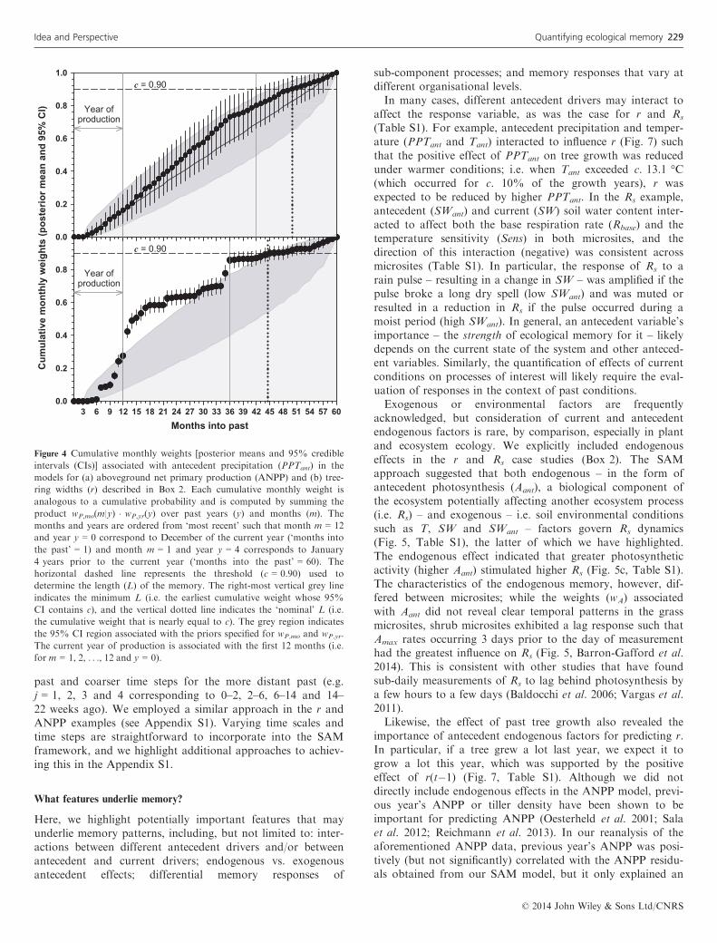
length of the memory. For example, the length of the ANPPprecipitation memory was c. 50 months, potentially spanning42–57 months (Fig. 4). That is, precipitation occurring morethan c. 50 months ago – or more than 38 months(c. 3.2 years) prior to the year of production – had little influ-ence on the current year’s ANPP. In the r example, the lengthof the memory varied depending on the driving variable (pre-cipitation vs. temperature). The precipitation memory for rwas c. 45 months, spanning 36–54 months (Fig. 4), and wasslightly shorter than that of ANPP, but the temperature mem-ory of r was comparatively long, c. 57 months, spanning anarrower range of possible values (50–57 months) (results notshown).

What time scales are important for quantifying memory?

Important to understanding the temporal features of memoryis the time scales specified for modelling the weights. Notethat we used nested weights in both the ANPP and r examples– yearly weights and monthly weights within each year – toaccount for memory patterns that reflect multiscale processes.In the ANPP example, the yearly w’s are well resolved(Fig. 2), while the monthly w’s are more uncertain (Fig. 4).Conversely, in the r example, each scale’s patterns are wellresolved (e.g. Fig. 4), and the monthly w’s suggest temporalmemory variability linked to seasonal climate variability. For

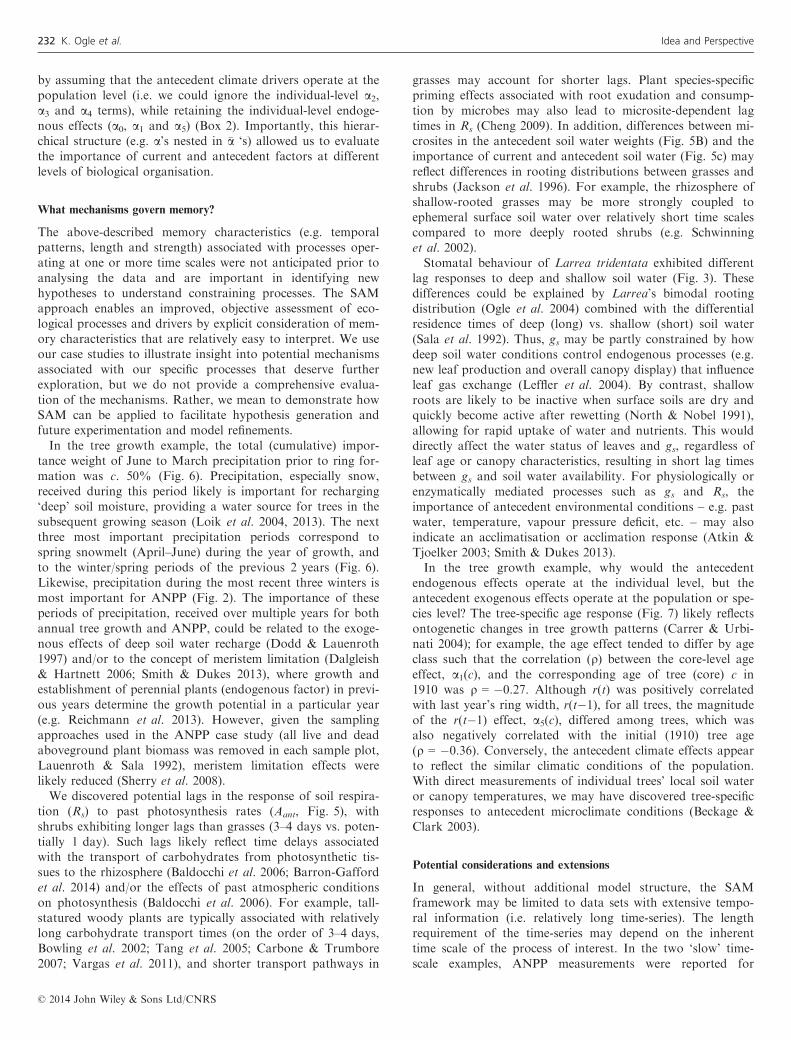
example, precipitation received during the winter prior to ringformation appears to be most important for understandingvariation in r for Pinus edulis at this site (Fig. 6). The monthlyw’s for temperature (wT,mo) are also fairly well resolved, but,unlike precipitation, they indicate that temperatures experi-enced during the previous summer are most important forpredicting r (Fig. 6). Thus, the nested weight model allows usto identify coarse time-scale memory patterns (e.g. the impor-tance of precipitation received during different years), and topartition these into memory effects that operate at finer timescales (e.g. the importance of precipitation received during dif-ferent seasonal periods).In the gs example, we took a different approach to accom-

modate varying time scales, which depends on the exogenousdriver of interest. For example, a ‘slow’ time scale wasassumed in computing antecedent deep soil water (W60ant)because the amount of deep soil water is expected to changerelatively slowly, and the response of gs to W60ant is likelymediated through ‘slow’ physiological and hormonal feed-backs (Ju et al. 2006; Saha et al. 2008). Conversely, a ‘fast’time scale is assumed for computing antecedent vapour pres-sure deficit (Dant) because stomata are directly exposed toatmospheric conditions, which vary at minute to hourlyscales, and they likely respond quickly to changes in vapourpressure deficit (Damour et al. 2010). Following Barron-Gafford et al. (2014), we only considered one time scale(daily) for Rs, and lags of similar time scales have been esti-mated for Rs in forest ecosystems (Vargas et al. 2011). Wehave found it useful, however, to employ varying, driver-dependent time scales, similar to the gs example, in otheranalyses of temporally extensive soil and ecosystem respira-tion data (e.g. Cable et al. 2013a), and for Rs data spanningmultiple years, longer (e.g. seasonal or yearly) memory effectsmay emerge from interactions with annual plant productivitydynamics (Janssens et al. 2001). In another study (Sondereg-ger et al. 2013), we allowed the time steps to vary such thatwe used relatively high resolution time steps for the recent

Days into the pastDays into the past

Impo

rtan

ce w

eigh

t (w

)

0.0

0.2

0.4

0.6

0.8

1.0

Hours into pastDays into the past1 2 3 4 5 6 7 0.5 1.0 1.5 2.0 2.5 3.00 1 2 3 4 5 61-2 3-4 5-6 6-7 7-8

w60 w30 wT wD(a) (b) (c) (d)

Figure 3 Importance weights (w) associated with stomatal conductance (gs) (Box 2). Posterior means (filled symbols) and 95% credible intervals (CIs) for

w’s associated with (a) antecedent deep (30–60 cm) soil water content (W60ant), where the antecedent time scale associated with the weights (w60) is defined

as blocks of multiple (2) days, (b) the daily weights (w30) associated with antecedent shallow (0–30 cm) soil water (W30ant), (c) the daily weights (wT)

associated with antecedent air temperature (Tant), and (d) the half-hourly weights (wD) associated with antecedent vapour pressure deficit (Dant). The prior

means and 95% CI are indicated by the horizontal black lines and the shaded grey regions, respectively.



past and coarser time steps for the more distant past (e.g.j = 1, 2, 3 and 4 corresponding to 0–2, 2–6, 6–14 and 14–22 weeks ago). We employed a similar approach in the r andANPP examples (see Appendix S1). Varying time scales andtime steps are straightforward to incorporate into the SAMframework, and we highlight additional approaches to achiev-ing this in the Appendix S1.

What features underlie memory?

Here, we highlight potentially important features that mayunderlie memory patterns, including, but not limited to: inter-actions between different antecedent drivers and/or betweenantecedent and current drivers; endogenous vs. exogenousantecedent effects; differential memory responses of

sub-component processes; and memory responses that vary atdifferent organisational levels.In many cases, different antecedent drivers may interact to

affect the response variable, as was the case for r and Rs

(Table S1). For example, antecedent precipitation and temper-ature (PPTant and Tant) interacted to influence r (Fig. 7) suchthat the positive effect of PPTant on tree growth was reducedunder warmer conditions; i.e. when Tant exceeded c. 13.1 °C(which occurred for c. 10% of the growth years), r wasexpected to be reduced by higher PPTant. In the Rs example,antecedent (SWant) and current (SW) soil water content inter-acted to affect both the base respiration rate (Rbase) and thetemperature sensitivity (Sens) in both microsites, and thedirection of this interaction (negative) was consistent acrossmicrosites (Table S1). In particular, the response of Rs to arain pulse – resulting in a change in SW – was amplified if thepulse broke a long dry spell (low SWant) and was muted orresulted in a reduction in Rs if the pulse occurred during amoist period (high SWant). In general, an antecedent variable’simportance – the strength of ecological memory for it – likelydepends on the current state of the system and other anteced-ent variables. Similarly, the quantification of effects of currentconditions on processes of interest will likely require the eval-uation of responses in the context of past conditions.Exogenous or environmental factors are frequently

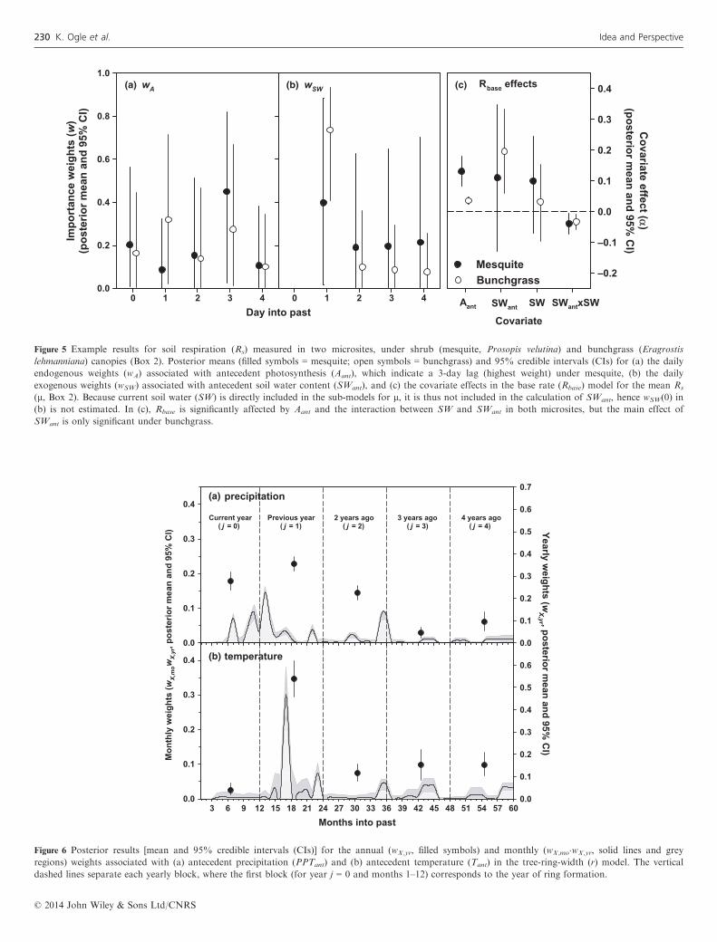
acknowledged, but consideration of current and antecedentendogenous factors is rare, by comparison, especially in plantand ecosystem ecology. We explicitly included endogenouseffects in the r and Rs case studies (Box 2). The SAMapproach suggested that both endogenous – in the form ofantecedent photosynthesis (Aant), a biological component ofthe ecosystem potentially affecting another ecosystem process(i.e. Rs) – and exogenous – i.e. soil environmental conditionssuch as T, SW and SWant – factors govern Rs dynamics(Fig. 5, Table S1), the latter of which we have highlighted.The endogenous effect indicated that greater photosyntheticactivity (higher Aant) stimulated higher Rs (Fig. 5c, Table S1).The characteristics of the endogenous memory, however, dif-fered between microsites; while the weights (wA) associatedwith Aant did not reveal clear temporal patterns in the grassmicrosites, shrub microsites exhibited a lag response such thatAmax rates occurring 3 days prior to the day of measurementhad the greatest influence on Rs (Fig. 5, Barron-Gafford et al.2014). This is consistent with other studies that have foundsub-daily measurements of Rs to lag behind photosynthesis bya few hours to a few days (Baldocchi et al. 2006; Vargas et al.2011).Likewise, the effect of past tree growth also revealed the

importance of antecedent endogenous factors for predicting r.In particular, if a tree grew a lot last year, we expect it togrow a lot this year, which was supported by the positiveeffect of r(t�1) (Fig. 7, Table S1). Although we did notdirectly include endogenous effects in the ANPP model, previ-ous year’s ANPP or tiller density have been shown to beimportant for predicting ANPP (Oesterheld et al. 2001; Salaet al. 2012; Reichmann et al. 2013). In our reanalysis of theaforementioned ANPP data, previous year’s ANPP was posi-tively (but not significantly) correlated with the ANPP residu-als obtained from our SAM model, but it only explained an

Months into past3 6 9 12 15 18 21 24 27 30 33 36 39 42 45 48 51 54 57 60

Cum

ulat

ive

mon

thly

wei

ghts

(pos

terio

r mea

n an

d 95

% C

I)

0.0

0.2

0.4

0.6

0.8

0.0

0.2

0.4

0.6

0.8

1.0c = 0.90

Year ofproduction

c = 0.90

Year ofproduction

Figure 4 Cumulative monthly weights [posterior means and 95% credible

intervals (CIs)] associated with antecedent precipitation (PPTant) in the

models for (a) aboveground net primary production (ANPP) and (b) tree-

ring widths (r) described in Box 2. Each cumulative monthly weight is

analogous to a cumulative probability and is computed by summing the

product wP,mo(m|y) � wP,yr(y) over past years (y) and months (m). The

months and years are ordered from ‘most recent’ such that month m = 12

and year y = 0 correspond to December of the current year (‘months into

the past’ = 1) and month m = 1 and year y = 4 corresponds to January

4 years prior to the current year (‘months into the past’ = 60). The

horizontal dashed line represents the threshold (c = 0.90) used to

determine the length (L) of the memory. The right-most vertical grey line

indicates the minimum L (i.e. the earliest cumulative weight whose 95%

CI contains c), and the vertical dotted line indicates the ‘nominal’ L (i.e.

the cumulative weight that is nearly equal to c). The grey region indicates

the 95% CI region associated with the priors specified for wP,mo and wP,yr.

The current year of production is associated with the first 12 months (i.e.

for m = 1, 2, . . ., 12 and y = 0).



Covariate

Covariate effect (α )

(posterior mean and 95%

CI)

—0.2

—0.1

0.0

0.1

0.2

0.3

0.4

Day into past

Impo

rtan

ce w

eigh

ts ( w

)(p

oste

rior m

ean

and

95%

CI)

0.0

0.2

0.4

0.6

0.8

1.0

0 1 2 3 4 0 1 2 3 4 Aant SWant SW SWantxSW

wSWwA Rbase effects

MesquiteBunchgrass

(a) (b) (c)

Figure 5 Example results for soil respiration (Rs) measured in two microsites, under shrub (mesquite, Prosopis velutina) and bunchgrass (Eragrostis

lehmanniana) canopies (Box 2). Posterior means (filled symbols = mesquite; open symbols = bunchgrass) and 95% credible intervals (CIs) for (a) the daily

endogenous weights (wA) associated with antecedent photosynthesis (Aant), which indicate a 3-day lag (highest weight) under mesquite, (b) the daily

exogenous weights (wSW) associated with antecedent soil water content (SWant), and (c) the covariate effects in the base rate (Rbase) model for the mean Rs

(l, Box 2). Because current soil water (SW) is directly included in the sub-models for l, it is thus not included in the calculation of SWant, hence wSW(0) in

(b) is not estimated. In (c), Rbase is significantly affected by Aant and the interaction between SW and SWant in both microsites, but the main effect of

SWant is only significant under bunchgrass.

Mon

thly

wei

ghts

( wX,mow

X,yr

, pos

terio

r mea

n an

d 95

% C

I)

0.0

0.1

0.2

0.3

0.4

Yearly weights (w

X,yr , posterior mean and 95%

CI)

0.0

0.1

0.2

0.3

0.4

0.5

0.6

0.7

Current year Previous year 2 years ago 3 years ago 4 years ago( j = 4)( j = 3)( j = 2)( j = 1)( j = 0)

3 6 9 12 15 18 21 24 27 30 33 36 39 42 45 48 51 54 57 600.0

0.1

0.2

0.3

0.4

Months into past

0.0

0.1

0.2

0.3

0.4

0.5

0.6temperature

precipitation(a)

(b)

Figure 6 Posterior results [mean and 95% credible intervals (CIs)] for the annual (wX,yr, filled symbols) and monthly (wX,mo�wX,yr, solid lines and grey

regions) weights associated with (a) antecedent precipitation (PPTant) and (b) antecedent temperature (Tant) in the tree-ring-width (r) model. The vertical

dashed lines separate each yearly block, where the first block (for year j = 0 and months 1–12) corresponds to the year of ring formation.



additional 2% of the variation in ANPP. This is in contrastto previous studies that found a stronger effect of previousyear’s ANPP (Oesterheld et al. 2001; Sala et al. 2012; Reich-mann et al. 2013), but unlike our flexible SAM approach,these studies assumed that only current and/or previous year’sprecipitation affected ANPP, and precipitation during eachmonth was treated as being equally important. Regardless, asillustrated in the Rs and r case studies, the SAM approachhighlighted the potentially critical role of endogenous factorsfor predicting the ecological processes of interest.In most ecological situations, the response of interest

reflects multiple, coupled sub-processes, each of which maypossess their own memory characteristics. In the gs and Rs

case studies, we expressed these responses as functions of twosub-components: a base-line response (e.g. gref or Rbase) andan environmental sensitivity term (e.g. Sens or Tsens) (Box 2).In both cases, each sub-component was significantly affectedby antecedent exogenous (gs and Rs) and endogenous (onlyapplicable to Rs) factors (Table S1). However, the directionand magnitude of the antecedent response varied betweensub-components. For example, antecedent temperature (Tant)significantly affected stomatal behaviour by influencing bothgref and Sens, but Tant had opposing effects on Sens and gref(Table S1). In addition, we assumed that antecedent vapourpressure deficit (Dant) only had the potential to influence Sens

(but not gref), reflecting a potential acclimation response ofstomata to the prevailing vapour pressure conditions. In theseexamples, we specified the antecedent drivers to share thesame temporal characteristics. For example, gref and Sensshared the same weights (wT) for antecedent temperature(Tant), and Rbase and Tsens shared the same weights (wA) forantecedent photosynthesis (Aant). Of course, the explicit char-acterisation of memory patterns in the form of the weights(w’s) makes the specification of different w’s easy, in principle,within the SAM framework.Different levels of organisation may also vary in their mem-

ory characteristics and responses to exogenous and endoge-nous drivers. The r case study nicely illustrates this because itincluded both individual-tree responses (via the a’s, Box 2)and associated population-level responses (via the �a‘s, Box 2).Interestingly, the direction and magnitude of the exogenouseffects of the antecedent climate variables (PPTant, Tant andPPTant 9 Tant) were consistent across trees (Fig. 7), indicatingthat the response to these antecedent variables may be anintrinsic property of the population or, more generally, thespecies. Conversely, the effects of tree age and previous ringwidths differed notably across trees (Fig. 7), implying thatsuch endogenous effects may be an inherent property of indi-vidual trees, which likely reflects an ontogenetic or genotypicsignal. This suggests that the model for r could be simplified

Inte

rcep

t0.0

0.2

0.4

0.6

0.8Core-level effectsPopulation-level

Age effect

—0.002

—0.001

0.000

0.001

0.002

0.003

PPT an

t effe

ct

0.00

0.01

0.02

0.03

0.04

Tant effect

0.00

0.02

0.04

0.06

0.08

0.10

0.12

Tree core (ordered from lowest to highest effect)

PPT an

txT an

t effe

ct

—0.04

—0.03

—0.02

—0.01 r(t-1) effect

0.0

0.2

0.4

0.6

0.8

Figure 7 Posterior means and 95% credible intervals (CIs) for the core- or tree-level (open symbols) and population-level (filled symbols) covariate effects

in the tree-ring width (r) model (Box 2). The horizontal dashed lines represent the zero line, and 95% CIs that overlap the zero line indicate non-significant

effects. The endogenous effects of tree age (Age) and the previous year’s ring width (r(t�1)) vary among trees (cores), whereas the exogenous effects of

antecedent precipitation (PPTant), antecedent temperature (Tant) and their interaction (PPTant 9 Tant) do not vary among trees.



by assuming that the antecedent climate drivers operate at thepopulation level (i.e. we could ignore the individual-level a2,a3 and a4 terms), while retaining the individual-level endoge-nous effects (a0, a1 and a5) (Box 2). Importantly, this hierar-chical structure (e.g. a’s nested in �a ‘s) allowed us to evaluatethe importance of current and antecedent factors at differentlevels of biological organisation.

What mechanisms govern memory?

The above-described memory characteristics (e.g. temporalpatterns, length and strength) associated with processes oper-ating at one or more time scales were not anticipated prior toanalysing the data and are important in identifying newhypotheses to understand constraining processes. The SAMapproach enables an improved, objective assessment of eco-logical processes and drivers by explicit consideration of mem-ory characteristics that are relatively easy to interpret. We useour case studies to illustrate insight into potential mechanismsassociated with our specific processes that deserve furtherexploration, but we do not provide a comprehensive evalua-tion of the mechanisms. Rather, we mean to demonstrate howSAM can be applied to facilitate hypothesis generation andfuture experimentation and model refinements.In the tree growth example, the total (cumulative) impor-

tance weight of June to March precipitation prior to ring for-mation was c. 50% (Fig. 6). Precipitation, especially snow,received during this period likely is important for recharging‘deep’ soil moisture, providing a water source for trees in thesubsequent growing season (Loik et al. 2004, 2013). The nextthree most important precipitation periods correspond tospring snowmelt (April–June) during the year of growth, andto the winter/spring periods of the previous 2 years (Fig. 6).Likewise, precipitation during the most recent three winters ismost important for ANPP (Fig. 2). The importance of theseperiods of precipitation, received over multiple years for bothannual tree growth and ANPP, could be related to the exoge-nous effects of deep soil water recharge (Dodd & Lauenroth1997) and/or to the concept of meristem limitation (Dalgleish& Hartnett 2006; Smith & Dukes 2013), where growth andestablishment of perennial plants (endogenous factor) in previ-ous years determine the growth potential in a particular year(e.g. Reichmann et al. 2013). However, given the samplingapproaches used in the ANPP case study (all live and deadaboveground plant biomass was removed in each sample plot,Lauenroth & Sala 1992), meristem limitation effects werelikely reduced (Sherry et al. 2008).We discovered potential lags in the response of soil respira-

tion (Rs) to past photosynthesis rates (Aant, Fig. 5), withshrubs exhibiting longer lags than grasses (3–4 days vs. poten-tially 1 day). Such lags likely reflect time delays associatedwith the transport of carbohydrates from photosynthetic tis-sues to the rhizosphere (Baldocchi et al. 2006; Barron-Gaffordet al. 2014) and/or the effects of past atmospheric conditionson photosynthesis (Baldocchi et al. 2006). For example, tall-statured woody plants are typically associated with relativelylong carbohydrate transport times (on the order of 3–4 days,Bowling et al. 2002; Tang et al. 2005; Carbone & Trumbore2007; Vargas et al. 2011), and shorter transport pathways in

grasses may account for shorter lags. Plant species-specificpriming effects associated with root exudation and consump-tion by microbes may also lead to microsite-dependent lagtimes in Rs (Cheng 2009). In addition, differences between mi-crosites in the antecedent soil water weights (Fig. 5B) and theimportance of current and antecedent soil water (Fig. 5c) mayreflect differences in rooting distributions between grasses andshrubs (Jackson et al. 1996). For example, the rhizosphere ofshallow-rooted grasses may be more strongly coupled toephemeral surface soil water over relatively short time scalescompared to more deeply rooted shrubs (e.g. Schwinninget al. 2002).Stomatal behaviour of Larrea tridentata exhibited different

lag responses to deep and shallow soil water (Fig. 3). Thesedifferences could be explained by Larrea’s bimodal rootingdistribution (Ogle et al. 2004) combined with the differentialresidence times of deep (long) vs. shallow (short) soil water(Sala et al. 1992). Thus, gs may be partly constrained by howdeep soil water conditions control endogenous processes (e.g.new leaf production and overall canopy display) that influenceleaf gas exchange (Leffler et al. 2004). By contrast, shallowroots are likely to be inactive when surface soils are dry andquickly become active after rewetting (North & Nobel 1991),allowing for rapid uptake of water and nutrients. This woulddirectly affect the water status of leaves and gs, regardless ofleaf age or canopy characteristics, resulting in short lag timesbetween gs and soil water availability. For physiologically orenzymatically mediated processes such as gs and Rs, theimportance of antecedent environmental conditions – e.g. pastwater, temperature, vapour pressure deficit, etc. – may alsoindicate an acclimatisation or acclimation response (Atkin &Tjoelker 2003; Smith & Dukes 2013).In the tree growth example, why would the antecedent

endogenous effects operate at the individual level, but theantecedent exogenous effects operate at the population or spe-cies level? The tree-specific age response (Fig. 7) likely reflectsontogenetic changes in tree growth patterns (Carrer & Urbi-nati 2004); for example, the age effect tended to differ by ageclass such that the correlation (q) between the core-level ageeffect, a1(c), and the corresponding age of tree (core) c in1910 was q = �0.27. Although r(t) was positively correlatedwith last year’s ring width, r(t�1), for all trees, the magnitudeof the r(t�1) effect, a5(c), differed among trees, which wasalso negatively correlated with the initial (1910) tree age(q = �0.36). Conversely, the antecedent climate effects appearto reflect the similar climatic conditions of the population.With direct measurements of individual trees’ local soil wateror canopy temperatures, we may have discovered tree-specificresponses to antecedent microclimate conditions (Beckage &Clark 2003).

Potential considerations and extensions

In general, without additional model structure, the SAMframework may be limited to data sets with extensive tempo-ral information (i.e. relatively long time-series). The lengthrequirement of the time-series may depend on the inherenttime scale of the process of interest. In the two ‘slow’ time-scale examples, ANPP measurements were reported for



50 years, and 91 growth rings were used for each tree. In thetwo ‘fast’ time-scale examples, gs and Rs were measured over16 and 27 non-consecutive days, respectively. While the gsand Rs time-series were discontinuous in time and may seemrelatively short, the sampling strategies resulted in data thatspanned a wide range of exogenous and/or endogenous condi-tions. However, significant efforts in developing large datasets associated with ecological structure and function (e.g.FLUXNET, TERN and NEON) will yield more long-termdata that will be available for rigorously quantifying ecologi-cal memory.We chose case studies from arid and semi-arid ecosystems

partly because these systems are likely to exhibit strong exoge-nous, and potentially endogenous, memory or legacy effects(e.g. Sala et al. 2012) given that they are often characterisedby highly variable ecological responses and environmentaldrivers (e.g. water and temperature). Our SAM approach,however, could be extended to understand the length, tempo-ral patterns, and strength of the memory in other extreme,more mesic, or potentially less variable systems. For example,SAM could be applied to boreal and arctic systems with stor-age-based hydrological dynamics, where the time scale forwhich soil moisture impacts plant and ecosystem carbon andwater fluxes is drawn out over multiple years such that cur-rent flux dynamics are likely controlled by prior freeze-thawcycles and permafrost degradation status (e.g. Iwata et al.2012; Cable et al. 2013b). SAM could also be used to evaluatethe antecedent exogenous and endogenous controls on thetiming and magnitude of green-up and flowering in tropicalforests, two globally important dynamic phenomena that arenot well understood (e.g. Pau et al. 2013; Krishnaswamy et al.2014; Morton et al. 2014). More generally, phenological pro-cesses are inherently temporal, and the rate and/or timing ofleaf-out or flowering may depend on past phonological sched-ules. Long-term data sets – such as the 700 + year cherryblossom record from Japan (Aono & Kazui 2008) or from theNational Phenology Network – could be used within theSAM framework to provide predictive ability of how ecologi-cal memory affects phenological processes, particularly in theface of changing climate. Moreover, we hypothesise that sys-tems characterised by little temporal variation in climate driv-ers are likely to be more strongly controlled by endogenousmemory (e.g. associated with effects of organismal size, pastproductivity, etc.) or exogenous disturbances (e.g. land-use orfire history), which could be tested with the SAM approach.

CONCLUSIONS

This study demonstrates that memory is important for under-standing contemporary ecological processes, and the length,temporal patterns, and strength of the memory can varygreatly among processes spanning a range of temporal andspatial scales. Importantly, the stochastic antecedent model-ling (SAM) framework provides an objective method for iden-tifying these latent memory properties by explicitlyquantifying antecedent exogenous and/or endogenous condi-tions and their effects on a diversity of ecological responses.We illustrated the utility of the SAM approach and the typesof unique insights it provides by applying it to four distinctly

different data sets that represent processes operating at sub-daily to interannual time scales. In all four examples, theSAM approach greatly improved our ability to predict theresponse of interest, revealing important lag periods and ante-cedent drivers. Although our examples were obtained fromarid and semi-arid systems, the SAM approach is expected tobe applicable to a diversity of systems characterised by tempo-ral variation in the response(s) of interest and associatedendogenous and/or exogenous drivers.Our SAM framework may also be broadly applicable within

and outside the field of ecology to understand the importanceof time, and memory in particular. Different ecological sub-disciplines use alternative descriptors to describe ecologicalmemory, such as ‘biological legacies’ (e.g. landscape ecology)and ‘antecedent effects’ (e.g. ecosystem ecology). The ecologi-cal memory concept is captured in notions of lag effects, timedelays, historical effects and buffering capacity (e.g. Bengtssonet al. 2003; Ogle & Reynolds 2004; Golinski et al. 2008;Schaefer 2009). The SAM approach provides a rigorous quan-titative approach for exploring these different aspects of mem-ory. Outside of ecology, memory has been used to describethe lag between atmospheric forcing and land surface hydrol-ogy (Koster & Suarez 2001; Lo & Famiglietti 2010), persis-tence of atmospheric chemical constituents (e.g. Varotsos &Kirk-Davidoff 2006) and changes in the physical structure ofbiological macromolecules (Yashima et al. 1999). Thus, thegeneral SAM formulation is expected to be applicable forquantifying memory of a diversity of dynamic processes repre-senting spatial and temporal scales spanning several orders ofmagnitude.

ACKNOWLEDGEMENTS

This work was supported by two DOE-NICCR grants (oneawarded to KO, TH, ML and DT, and another awarded toKO), two NSF grants (NSF-DEB 0415977 and NSF-IOS0418134 awarded to TH), a US National Park Service grant(DT, ML), and the Philecology Foundation of Fort WorthTexas (TH and GBG), and the Irvine Company (TH). Wealso thank Rich Lucas and Stan Smith for discussions contri-buting to our SAM approach.

AUTHORSHIP STATEMENT

K.O. led all aspects of the study; K.O., J.J.B., G.A.B-G.,L.P.B. and J.M.Y contributed to testing and applying theSAM framework with real data; G.A.B.-G., T.E.H and K.O.contributed data; all co-authors contributed to the develop-ment of the conceptual ideas and to writing the manuscript.

REFERENCES

Aono, Y. & Kazui, K. (2008). Phenological data series of cherry tree

flowering in Kyoto, Japan, and its application to reconstruction of

springtime temperatures since the 9th century. Int. J. Climatol., 28,

905–914.Atkin, O.K. & Tjoelker, M.G. (2003). Thermal acclimation and the

dynamic response of plant respiration to temperature. Trends Plant

Sci., 8, 343–351.



Baldocchi, D., Tang, J.W. & Xu, L.K. (2006). How switches and lags in

biophysical regulators affect spatial-temporal variation of soil

respiration in an oak-grass savanna. J. Geophys Res., 111, G02008,

doi:10.1029/2005JG000063.

Bardgett, R.D., Bowman, W.D., Kaufmann, R. & Schmidt, S.K. (2005).

A temporal approach to linking aboveground and belowground

ecology. Trends Ecol. Evol., 20, 634–641.Barron-Gafford, G.A., Scott, R.L., Jenerette, G.D. & Huxman, T.E.

(2011). The relative controls of temperature, soil moisture, and plant

functional group on soil CO2 efflux at diel, seasonal, and annual scales.

J. Geophys Res-Biogeo., 116, G01023, doi:10.1029/2010JG001442.

Barron-Gafford, G., Cable, J.M., Patrick-Bentley, L.D., Scott, R.L.,

Huxman, T.E., Jenerette, G.D. et al. (2014). Quantifying the timescales

over which exogenous and endogenous conditions affect soil

respiration. New Phytol., 202, 442–454.Beckage, B. & Clark, J.S. (2003). Seedling survival and growth of three

forest tree species: the role of spatial heterogeneity. Ecology, 84, 1849–1861.

Bengtsson, J., Angelstam, P., Elmqvist, T., Emanuelsson, U., Folke, C.,

Ihse, M. et al. (2003). Reserves, resilience and dynamic landscapes.

Ambio, 32, 389–396.Bowling, D.R., McDowell, N.G., Bond, B.J., Law, B.E. & Ehleringer,

J.R. (2002). 13C content of ecosystem respiration is linked to

precipitation and vapor pressure deficit. Oecologia, 131, 113–124.Cable, J.M., Ogle, K., Williams, D.G., Weltzin, J.F. & Huxman, T.E.

(2008). Soil texture drives responses of soil respiration to precipitation

pulses in the Sonoran Desert: implications for climate change.

Ecosystems, 11, 961–979.Cable, J.M., Ogle, K., Barron-Gafford, G.A., Bentley, L.P., Cable, W.L.,

Scott, R.L. et al. (2013a). Antecedent conditions influence soil respiration

differences in shrub and grass patches. Ecosystems, 16, 1230–1247.Cable, J.M., Ogle, K., Bolton, W.R., Bentley, L.P., Romanovsky, V.,

Iwata, H. et al. (2013b). Permafrost thaw affects boreal deciduous

plant transpiration through increased soil water, deeper thaw, and

warmer soils. Ecohyrdology, doi:10.1002/eco.1423, 221-233.

Carbone, M.S. & Trumbore, S.E. (2007). Contribution of new

photosynthetic assimilates to respiration by perennial grasses and shrubs:

residence times and allocation patterns.New Phytol., 176, 124–135.Carrer, M. & Urbinati, C. (2004). Age-dependent tree-ring growth responses

to climate in Larix decidua and Pinus cembra. Ecology, 85, 730–740.Chave, J. (2013). The problem of pattern and scale in ecology: what have

we learned in 20 years? Ecol. Lett., 16, 4–16.Cheng, W. (2009). Rhizosphere priming effect: its functional relationships

with microbial turnover, evapotranspiration, and C-N budgets. Soil

Biol. Biochem., 41, 1795–1801.Coops, N.C., Jassal, R.S., Leuning, R., Black, A.T. & Morgenstern, K.

(2007). Incorporation of a soil water modifier into MODIS predictions

of temperate Douglas-fir gross primary productivity: initial model

development. Agric. For. Meteorol., 147, 99–109.Crooks, J.A. (2005). Lag times and exotic species: the ecology and

management of biological invasions in slow-motion. Ecoscience, 12,

316–329.Dalgleish, H.J. & Hartnett, D.C. (2006). Below-ground bud banks increase

along a precipitation gradient of the North American Great Plains: a test

of the meristem limitation hypothesis. New Phytol., 171, 81–89.Damour, G., Simonneau, T., Cochard, H. & Urban, L. (2010). An

overview of models of stomatal conductance at the leaf level. Plant,

Cell Environ., 33, 1419–1438.Dodd, M.B. & Lauenroth, W.K. (1997). The influence of soil texture on

the soil water dynamics and vegetation structure of a shortgrass steppe

ecosystem. Plant Ecol., 133, 13–28.Druckenbrod, D.L. (2005). Dendroecological reconstructions of forest

disturbance history using time-series analysis with intervention

detection. Can. J. For. Res., 35, 868–876.Elzinga, J.A., Atlan, A., Biere, A., Gigord, L., Weis, A.E. & Bernasconi,

G. (2007). Time after time: flowering phenology and biotic interactions.

Trends Ecol. Evol., 22, 432–439.

Fierer, N., Colman, B.P., Schimel, J.P. & Jackson, R.B. (2006). Predicting

the temperature dependence of microbial respiration in soil: a

continental-scale analysis. Global Biogeochem. Cycles, 20, Gb3026: doi:

10.1029/2005gb002644.

Fritts, H.C. (1966). Growth-rings of trees: their correlation with climate.

Science, 154, 973–979.Gagen, M., McCarroll, D. & Edouard, J.L. (2004). Latewood width,

maximum density, and stable carbon isotope ratios of pine as climate

indicators in a dry subalpine environment, French Alps. Arct. Antarct.

Alp. Res., 36, 166–171.Gelman, A., Carlin, J.B., Stern, H.S. & Rubin, D.B. (2004). Bayesian

Data Analysis. Chapman and Hall/CRC Press, Boca Raton.

Golinski, M., Bauch, C. & Arland, M. (2008). The effects of endogenous

ecological memory on population stability and resilience in a variable

environment. Ecol. Model., 212, 334–341.Graumlich, L.J. (1991). Subalpine tree growth, climate, and increasing

CO2: an assessment of recent growth trends. Ecology, 72, 1–11.Griesbauer, H.P. & Green, D.S. (2010). Assessing the climatic sensitivity

of Douglas-fir at its northern range margins in British Columbia,

Canada. Trees, 24, 375–389.Hawkins, T.W. & Ellis, A.W. (2010). The dependence of streamflow on

antecedent subsurface moisture in an arid climate. J. Arid Environ., 74,

75–86.ITRDB (2007). Contributors of the International Tree-Ring Data Bank.

URL http://www.ncdc.noaa.gov/paleo/treering.html

Iwata, H., Harazono, Y. & Ueyama, M. (2012). The role of permafrost in

water exchange of a black spruce forest in Interior Alaska. Agric. For.

Meteorol., 161, 107–115.Jackson, R.B., Canadell, J., Ehleringer, J.R., Mooney, H.A., Sala, O.E. &

Schulze, E.D. (1996). A global analysis of root distributions for

terrestrial biomes. Oecologia, 108, 389–411.Janssens, I.A., Lankreijer, H., Matteucci, G., Kowalski, A.S., Buchmann,

N., Epron, D. et al. (2001). Productivity overshadows temperature in

determining soil and ecosystem respiration across European forests.

Glob. Change Biol., 7, 269–278.Johnson, E.A. & Miyanishi, K. (2008). Testing the assumptions of

chronosequences in succession. Ecol. Lett., 11, 419–431.Ju, W.M., Chen, J.M., Black, T.A., Barr, A.G., Liu, J. & Chen, B.Z.

(2006). Modelling multi-year coupled carbon and water fluxes in a

boreal aspen forest. Agric. For. Meteorol., 140, 136–151.Koster, R.D. & Suarez, M.J. (2001). Soil moisture memory in climate

models. J. Hydrometeorol., 2, 558–570.Kreyling, J., Beierkuhnlein, C. & Jentsch, A. (2010). Effects of soil freeze-

thaw cycles differ between experimental plant communities. Basic Appl.

Ecol., 11, 65–75.Krishnaswamy, J., Robert, J. & Shijo, J. (2014). Consistent response of

vegetation dynamics to recent climate change in tropical mountain

regions. Glob. Change Biol., 20, 203–215.Lauenroth, W.K. & Sala, O.E. (1992). Long-term forage production of

North American shortgrass steppe. Ecol. Appl., 2, 397–403.Leffler, A.J., Ivans, C.Y., Ryel, R.J. & Caldwell, M.M. (2004).

Gas exchange and growth responses of the desert shrubs

Artemisia tridentata and Chrysothamnus nauseosus to shallow- vs.

deep-soil water in a glasshouse experiment. Environ. Exp. Bot.,

51, 9–19.Leuning, R., Cleugh, H.A., Zegelin, S.J. & Hughes, D. (2005).

Carbon and water fluxes over a temperate Eucalyptus forest and a

tropical wet/dry savanna in Australia: measurements and

comparison with MODIS remote sensing estimates. Agric. For.

Meteorol., 129, 151–173.Levin, S.A. (1992). The problem of pattern and scale in ecology. Ecology,

73, 1943–1967.Lo, M.H. & Famiglietti, J.S. (2010). Effect of water table dynamics on

land surface hydrologic memory. J. Geophys Res., 115, D22118.

doi:10.1029/2010jd014191.

Loik, M.E., Breshears, D.D., Lauenroth, W.K. & Belnap, J. (2004). A

multi-scale perspective of water pulses in dryland ecosystems:



climatology and ecohydrology of the western USA. Oecologia, 141,

269–281.Loik, M.E., Griffith, A.B. & Alpert, H. (2013). Impacts of long-term

snow climate change on a high-elevation cold desert shrubland,

California, USA. Plant Ecol., 214, 255–266.Lundberg, J. & Moberg, F. (2003). Mobile link organisms and ecosystem

functioning: implications for ecosystem resilience and management.

Ecosystems, 6, 87–98.Monserud, R.A. & Marshall, J.D. (2001). Time-series analysis of d13C

from tree rings. I. Time trends and autocorrelation. Tree Physiol., 21,

1087–1102.Morton, D.C., Nagol, J., Carabajal, C.C., Rosette, J., Palace, M., Cook,

B.D. et al. (2014). Amazon forests maintain consistent canopy structure

and greenness during the dry season. Nature, 506, 221–224.North, G.B. & Nobel, P.S. (1991). Changes in hydraulic conductivity and

anatomy caused by drying and rewetting roots of Agave deserti

(Agavaceae). Am. J. Bot., 78, 906–915.Oesterheld, M., Loreti, J., Semmartin, M. & Sala, O.E. (2001). Inter-

annual variation in primary production of a semi-arid grassland related

to previous-year production. J. Veg. Sci., 12, 137–142.Ogle, K. & Barber, J.J. (2008). Bayesian data-model integration in plant

physiological and ecosystem ecology. Prog. Botany, 69, 281–311.Ogle, K. & Reynolds, J.F. (2002). Desert dogma revisited: coupling of

stomatal conductance and photosynthesis in the desert shrub, Larrea

tridentata. Plant, Cell Environ., 25, 909–921.Ogle, K. & Reynolds, J.F. (2004). Plant responses to precipitation in

desert ecosystems: integrating functional types, pulses, thresholds, and

delays. Oecologia, 141, 282–294.Ogle, K., Wolpert, R.L. & Reynolds, J.F. (2004). Reconstructing plant

root area and water uptake profiles. Ecology, 85, 1967–1978.Padisak, J. (1992). Seasonal auccession of phytoplankton in a large

shallow lake (Balaton, Hungary) - a dynamic approach to ecological

memory, its possible role and mechanisms. J. Ecol., 80, 217–230.Patrick, L.D., Ogle, K., Bell, C.W., Zak, J. & Tissue, D. (2009).

Physiological responses of two contrasting desert plant species to

precipitation variability are differentially regulated by soil moisture and

nitrogen dynamics. Glob. Change Biol., 15, 1214–1229.Pau, S., Wolkovich, E.M., Cook, B.I., Nytch, C.J., Regetz, J.,

Zimmerman, J.K. et al. (2013). Clouds and temperature drive dynamic

changes in tropical flower production. Nat. Clim. Change, 3, 838–842.Peterson, G.D. (2002). Contagious disturbance, ecological memory, and

the emergence of landscape pattern. Ecosystems, 5, 329–338.Reichmann, L.G., Sala, O.E. & Peters, D.P.C. (2013). Precipitation

legacies in desert grassland primary production occur through previous-

year tiller density. Ecology, 94, 435–443.Resco, V., Hartwell, J. & Hall, A. (2009). Ecological implications of

plants’ ability to tell the time. Ecol. Lett., 12, 583–592.Saha, S., Strazisar, T.M., Menges, E.S., Ellsworth, P. & Sternberg, L.

(2008). Linking the patterns in soil moisture to leaf water potential,

stomatal conductance, growth, and mortality of dominant shrubs in the

Florida scrub ecosystem. Plant Soil, 313, 113–127.Sala, O.E., Lauenroth, W.K. & Parton, W.J. (1992). Long-term soil water

dynamics in the shortgrass steppe. Ecology, 73, 1175–1181.Sala, O.E., Gherardi, L.A., Reichmann, L., Jobbagy, E. & Peters, D.

(2012). Legacies of precipitation fluctuations on primary production:

theory and data synthesis. Philos. Trans. R. Soc. B, 367, 3135–3144.Schaefer, V. (2009). Alien invasions, ecological restoration in cities and

the loss of ecological memory. Restor. Ecol., 17, 171–176.

Schwinning, S. & Sala, O.E. (2004). Hierarchy of responses to resource

pulses in and semi-arid ecosystems. Oecologia, 141, 211–220.Schwinning, S., Davis, K., Richardson, L. & Ehleringer, J.R. (2002).

Deuterium enriched irrigation indicates different forms of rain use

in shrub/grass species of the Colorado Plateau. Oecologia, 130, 345–355.

Sherry, R.A., Weng, E.S., Arnone, J.A., Johnson, D.W., Schimel, D.S.,

Verburg, P.S. et al. (2008). Lagged effects of experimental warming

and doubled precipitation on annual and seasonal aboveground

biomass production in a tallgrass prairie. Glob. Change Biol., 14, 2923–2936.

Shim, J.H., Pendall, E., Morgan, J.A. & Ojima, D.S. (2009). Wetting and

drying cycles drive variations in the stable carbon isotope ratio of

respired carbon dioxide in semi-arid grassland. Oecologia, 160, 321–333.Smith, N.G. & Dukes, J.S. (2013). Plant respiration and photosynthesis in

global-scale models: incorporating acclimation to temperature and

CO2. Glob. Change Biol., 19, 45–63.Sonderegger, D., Ogle, K., Evans, R.D., Nowak, R.S. & Ferguson, S.

(2013). Temporal dynamics of root growth under long-term exposure to

elevated CO2 in the Mojave Desert. New Phytol., 138, 127–138.Spiegelhalter, D.J., Best, N.G., Carlin, B.R. & van der Linde, A. (2002).

Bayesian measures of model complexity and fit. J. Roy. Stat. Soc. B,

64, 583–616.Tang, J.W., Baldocchi, D.D. & Xu, L. (2005). Tree photosynthesis

modulates soil respiration on a diurnal time scale. Glob. Change Biol.,

11, 1298–1304.Tingley, M.P., Craigmile, P.F., Haran, M., Li, B., Mannshardt, E. &

Rajaratnam, B. (2012). Piecing together the past: statistical insights into

paleoclimatic reconstructions. Quatern. Sci. Rev., 35, 1–22.Vargas, R., Baldocchi, D.D., Bahn, M., Hanson, P.J., Hosman, K.P.,

Kulmala, L. et al. (2011). On the multi-temporal correlation between

photosynthesis and soil CO2 efflux: reconciling lags and observations.

New Phytol., 191, 1006–1017.Varotsos, C. & Kirk-Davidoff, D. (2006). Long-memory processes in

ozone and temperature variations at the region 60o S-60o N. Atmos.

Chem. Phys., 6, 4093–4100.Visser, M.E. & Both, C. (2005). Shifts in phenology due to global climate

change: the need for a yardstick. Proc. Biol. Sci., 272, 2561–2569.Woodhouse, C.A., Gray, S.T. & Meko, D.M. (2006). Updated streamflow

reconstructions for the Upper Colorado River Basin. Water Resour.

Res., 42, W05415.

Yashima, E., Maeda, K. & Okamoto, Y. (1999). Memory of

macromolecular helicity assisted by interaction with achiral small

molecules. Nature, 399, 449–451.

SUPPORTING INFORMATION

Additional Supporting Information may be downloaded viathe online version of this article at Wiley Online Library(www.ecologyletters.com).

Editor, Elsa ClelandManuscript received 5 June 2014First decision made 18 July 2014Manuscript accepted 7 November 2014



Documents

Quantifying ecological memory in plant and …...IDEA AND PERSPECTIVE Quantifying ecological memory in plant and ecosystem processes Kiona Ogle,1* Jarrett J. Barber,2 Greg A. Barron-Gafford,3