Quantifying Marine Microbes: A Simulation to …cmore.soest.hawaii.edu/downloads/2010_quantifying_random...Marine microbes are extremely abundant organisms; a single liter of sea water

American Society for Microbiology Education Department 1752 N Street, NW Washington, DC 20036 [email protected]

Microbial Discovery Activity Quantifying Marine Microbes: A Simulation to Introduce Random Sampling

Authors Barbara Bruno1, Kimberly Tice1, Kate Achilles1 & Joan Matsuzaki2 1Center for Microbial Oceanography: Research and Education, Honolulu, HI 2President Theodore Roosevelt High School, Honolulu, HI [email protected]

Intended Audience K-4 5-8 X 9-12 X

Activity Characteristics

Class room setting X Requires special equipment Uses hands-on manipulatives X Requires mathematical skills X Can be performed individually Requires group work X Requires more than (45 min) class period Appropriate for special needs student X

barb

Text Box

http://www.asm.org/asm/images/MDA-PDF/2010%20marine%20microbes.pdf

ASM Microbial Discovery Activity Quantifying Marine Microbes: A Simulation to Introduce Random Sampling

Page 2

Introduction Description In this activity, students learn about the abundance and diversity of marine microbes, and then randomly sample simulated “marine microbes” to understand how scientists quantify the abundance of these organisms.

Abstract This lesson introduces random sampling, one of the key concepts employed by scientists to study the natural environment, including microbial communities. Students first learn about the abundance and diversity of marine microbes. Colored beads in a bag are then used to represent different types of microbes, with the bag itself representing the ocean. Working in groups, each student randomly samples ten “microbes” from the “ocean”, and records the data. To learn about the inherent variability of random sampling, the students then compare the composition of their individual samples, their group’s pooled sample data, and that of the entire population.

Core Themes Addressed General Microscopy Concepts Microbial Cell Biology Microbial Genetics Microorganisms and Humans Microorganisms and the Environment Microbial Evolution and Diversity X Other –Environmental Sampling X

Keywords Diversity, statistics, counting, microbial abundance

Learning Objectives At the completion of this activity, the learner will:

1. Gain an appreciation of the vast abundance and diversity of marine microbes. 2. Understand how and why scientists obtain random samples. 3. Understand that large samples tend to more closely approximate population parameters.


Page 3

National Science Education Standards Addressed Standard A: Science as Inquiry – Students will conduct a guided scientific investigation to quantify the composition of a simulated marine microbial community. Standard C: Life Sciences – Students will learn about the diversity of marine microbes, including the environments they inhabit, and the diverse adaptations and functions that allow them to survive in these environments. Standard F: Science in Personal and Social Perspectives – Students will learn about random sampling, a technique commonly used to quantify and monitor changes in population size, an important measure of environmental health.


Page 4

TTTeeeaaaccchhheeerrr HHHaaannndddooouuuttt QQQuuuaaannntttiiifffyyyiiinnnggg MMMaaarrriiinnneee MMMiiicccrrrooobbbeeesss::: AAA SSSiiimmmuuulllaaatttiiiooonnn tttooo IIInnntttrrroooddduuuccceee

RRRaaannndddooommm SSSaaammmpppllliiinnnggg

Student Prior Knowledge This activity requires that students be comfortable with arithmetic, including the calculation of percentages.

Teacher Background Information Marine microbes are extremely abundant organisms; a single liter of sea water can contain more than a billion of these amazing creatures. Because they are so abundant, it is impossible to learn about the size of marine microbe populations by counting the organisms individually. Instead, scientists quantify marine microbes using a process called sampling. In fact, sampling is used to estimate the population sizes of all kinds of organisms that are too numerous to count, such as snails in the rocky intertidal zone or spiders in the forest. Sampling is the process by which a subset of a population is quantified, and that subset is used to make inferences about the total population. For example, to quantify the abundance of a type of microbe called diatoms, a scientist might take 10 seawater samples of 1 ml each, and quantify the number of diatoms in each sample. The scientist could then calculate the average number of diatoms per milliliter of seawater, and multiply by 1000 to get an estimate of the number in a liter of seawater. Similar procedures can be used, for example, in the rocky intertidal zone. There, scientists may quantify the number of snails in 10 plots each of size 1 m2. The average number of snails in all of the plots could then be used to estimate the total number of snails within that entire intertidal site. Because the numbers of organisms in a single sample can vary widely, the accuracy of the estimate tends to increase as you increase the number and/or size of samples taken. However, at some point, a small increase in accuracy is not worth the extra work required. Thus, scientists must weigh this trade-off and decide what their sample size should be to get an acceptable population estimate. When taking samples, it is important not to introduce bias, for example by choosing to take samples in only the shallowest part of the intertidal zone. For this reason, scientists often use what are called random samples. Random samples are chosen by a method involving an unpredictable component, so that all members of the population have an equal chance of being selected as part of the sample. In this activity, students will take random samples of simulated marine microbes to make inferences about their abundance in the total population.

Class Time This lesson will require a minimum of one 45 minute class period.

1. Students will be provided with the Student Reading called “An Introduction to Marine Microbes.” This reading can be assigned the previous evening as homework, or can be read during the first 5-10 minutes of class.


Page 5

2. The next 5-10 minutes will be spent briefly discussing the reading and introducing students to the concept of random sampling.

3. Students will then be provided with the Student Handout and Student Datasheet. They will spend 20-30 minutes randomly sampling their microbe population, and filling in the data tables on the Student Datasheet.

4. The questions at the end of the Student Datasheet, which should take approximately 15 minutes to complete, may be finished as homework if there is not sufficient class time.

Teacher Preparation Time This lesson will require approximately 30 minutes of preparation time.

1. Make one copy of the Student Reading, Student Handout and Student Datasheet for each student.

2. Determine how many groups of students you will have. We recommend that students work in groups of 4.

3. Decide what objects you would like to use to represent marine microbes. Any small object that comes in different colors will do, such as colored beads.

4. You will need one Ziploc bag for each group of students. Fill each bag with 300 beads, using the color distribution listed below under Materials.

Materials and Equipment For each group of students, the following materials are needed:

1. One Ziploc bag 2. 300 beads (or other small objects), with the following color distribution:

White – 105 Red – 75 Green – 45 Pink – 45 Blue – 24 Purple – 6 3. Sorting tray (any tray or plate that will prevent the beads from rolling away) 4. 6 small storage containers

Methods Introduction

1. Pass out the Student Reading. This reading introduces students to marine microbes, and will help them appreciate the sheer abundance and diversity of these microorganisms.

2. After students complete the reading, begin a class discussion. Given that microbes are so abundant, ask your students how they would study marine microbe populations if they were microbial oceanographers. Could they count all of the microbes in the ocean? What about in a single bay? Since there are more than a billion microbes in just one liter of water, there is no way to count all of the microbes in a given population.

3. Explain briefly that scientists use a technique called random sampling to quantify the population sizes of species within an ecosystem when it is not possible or practical to count all the individuals.

4. Explain to the students that they are going to become microbial oceanographers. They will use random sampling to determine the relative abundance of different types of “microbes” in the “ocean”.


Page 6

5. Hold up one Ziploc bag of beads. Explain that the bag represents the ocean, and the beads it contains represent the population of all microbes in the ocean. Each plastic bead represents an individual microbe, and each color is meant to represent a different type of microbe. Each group of students will be studying microbe populations just like this one.

6. Remind students that the numbers of microbes in our imaginary ocean are fabricated to illustrate the concept of random sampling, and are not intended to reflect the actual abundances of these microbes in the Earth’s oceans. The data do, however, generally reflect the relative ranking of abundances of these different types of microbes.

7. Pass out the Student Handout and Student Datasheet (one per student). On the datasheet, have students look at Table 1 and note which type of microbe is represented by each color of bead.

8. Divide the class into groups and assign each group to a table. 9. Distribute one set of materials (1 bag of beads, 1 sorting tray, and 6 storage containers) to

each group. 10. Have each student complete the hypothesis at the top of the datasheet, based on their

observation of their Ziploc bag of “microbes”. For example, “The most abundant type of microbe (bead) in the ocean (bag) is bacteria (red).”

Data Collection: Table 1 (Sample Data)

1. Have students follow the directions on the handout under Data Collection: Table 1. You can either walk your students through each step, or have them work independently in their groups.

2. When students are finished, bring the class together to ensure that they completed Table 1 correctly before proceeding. Note that answers will vary, but each group should have:

a. Row totals equal to 10 for each student (e.g., H2=10, H3=10, H4=10, etc.). b. In line 11, the sum of the group totals for each microbe (e.g., B11, C11, D11, etc.)

should equal the grand total (H11). c. Grand total (H11) equal to 40 (or 10 times the number of students in each group). d. In line 12, the sum of all group percentages (H12) should add up to 100% (within

rounding error). 3. An example is given in the Answer Key to Student Datasheet. 4. Explain that scientists are constantly revising their methods and hypotheses based on new

data. Ask the students if they feel they should revise their initial hypothesis based on Table 1 results. If so, have them write their revised hypothesis on the datasheet. If not, have students explain why they chose to retain their hypothesis.

Data Collection: Table 2 (Population Data)

1. Now the students will count the entire population of all microbes in the ocean (that is, take a census) by following the instructions on their handout under Data Collection: Table 2. Again, you can either walk your students through each step, or have them work independently in their groups.

2. Note that, unlike Table 1, answers will not vary for Table 2. The entire population for each group should total 300 and have the same color distribution as listed in the Answer Key to the Student Datasheet. Review each group’s totals. If any of their answers differ, have the group recount their beads and/or search the area for missing beads.

Questions

1. Have students answer questions 1-7 on the Student Datasheet. This may need to be completed as homework.


Page 7

Delivery This exercise can be run as a teacher-led activity or student-teamed activity. We recommend students work in groups of four.

Technology Utilization If desired, students may use calculators in this activity.

Microorganisms No microorganisms are used in this activity.

Safety Issues Students will be working with small objects, such as plastic beads. These can pose a choking hazard, so it is important that students do not place these objects in their mouths.

Assessment and Evaluation of Activity The included Student Datasheet can be used to formally assess student learning.

Possible Modifications The colors of the objects used in this activity can be changed to those of objects you have on hand. If objects of different colors are used, make sure to modify the colors on Tables 1 and 2.

References The random sampling lesson is based on a non-microbial lesson developed by Our Project in Hawaii’s Intertidal (http://www.hawaii.edu/gk-12/opihi/classroom_home.shtml). The microbial information is based on Key Concepts in Microbial Oceanography (http://cmore.soest.hawaii.edu/downloads/MO_key_concepts_hi-res.pdf). References for the student reading are cited in the text.


Page 8

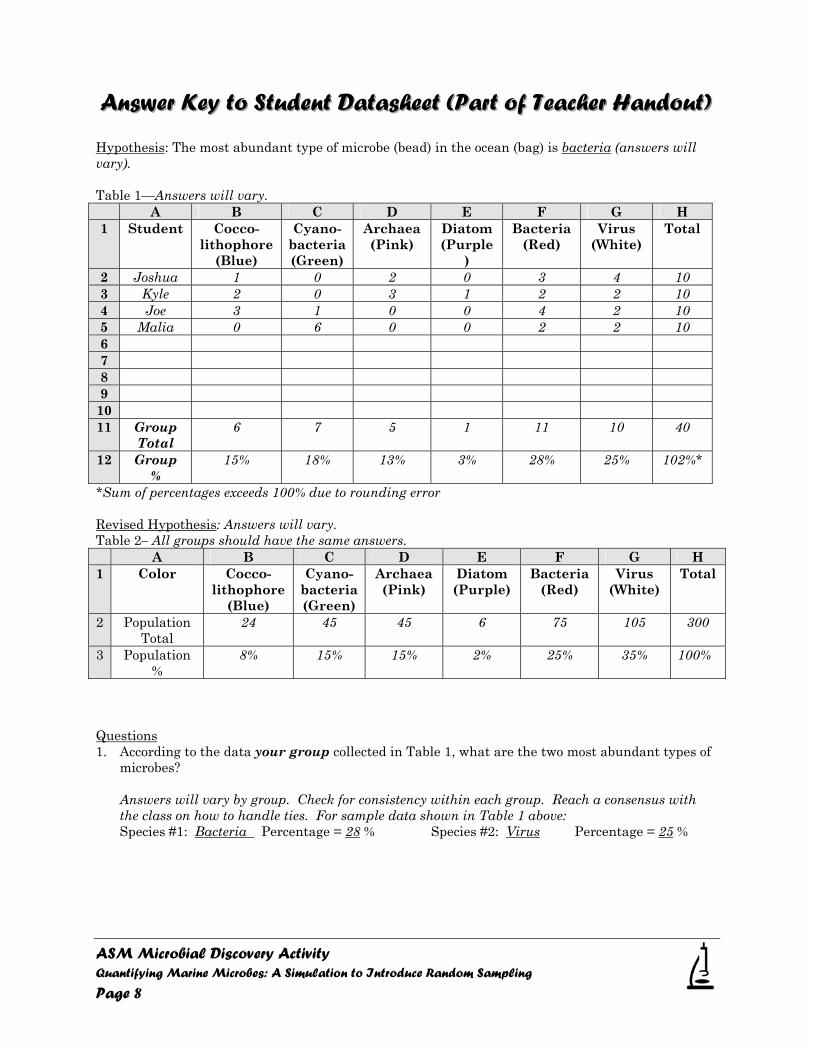
AAAnnnssswwweeerrr KKKeeeyyy tttooo SSStttuuudddeeennnttt DDDaaatttaaassshhheeeeeettt (((PPPaaarrrttt ooofff TTTeeeaaaccchhheeerrr HHHaaannndddooouuuttt))) Hypothesis: The most abundant type of microbe (bead) in the ocean (bag) is bacteria (answers will vary). Table 1—Answers will vary.

A B C D E F G H 1 Student Cocco-

lithophore (Blue)

Cyano-bacteria (Green)

Archaea (Pink)

Diatom (Purple

)

Bacteria (Red)

Virus (White)

Total

2 Joshua 1 0 2 0 3 4 10 3 Kyle 2 0 3 1 2 2 10 4 Joe 3 1 0 0 4 2 10 5 Malia 0 6 0 0 2 2 10 6 7 8 9

10 11 Group

Total 6 7 5 1 11 10 40

12 Group %

15% 18% 13% 3% 28% 25% 102%*

*Sum of percentages exceeds 100% due to rounding error Revised Hypothesis: Answers will vary. Table 2– All groups should have the same answers. A B C D E F G H

1 Color Cocco-lithophore

(Blue)


Archaea (Pink)

Diatom (Purple)

Bacteria (Red)

Virus (White)

Total

2 Population Total

24 45 45 6 75 105 300

3 Population %

8% 15% 15% 2% 25% 35% 100%

Questions 1. According to the data your group collected in Table 1, what are the two most abundant types of

microbes? Answers will vary by group. Check for consistency within each group. Reach a consensus with the class on how to handle ties. For sample data shown in Table 1 above: Species #1: Bacteria Percentage = 28 % Species #2: Virus Percentage = 25 %


Page 9

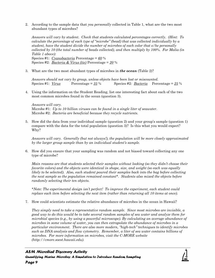
2. According to the sample data that you personally collected in Table 1, what are the two most abundant types of microbes?

Answers will vary by student. Check that students calculated percentages correctly. (Hint: To calculate the percentage of each type of “microbe” (bead) that was collected individually by a student, have the student divide the number of microbes of each color that s/he personally collected by 10 (the total number of beads collected), and then multiply by 100%. For Malia (in Table 1 above): Species #1: Cyanobacteria Percentage = 60 % Species #2: Bacteria & Virus (tie) Percentage = 20 %

3. What are the two most abundant types of microbes in the ocean (Table 2)?

Answers should not vary by group, unless objects have been lost or miscounted. Species #1: Virus Percentage = 35 % Species #2: Bacteria Percentage = 25 %

4. Using the information on the Student Reading, list one interesting fact about each of the two

most common microbes found in the ocean (question 3).

Answers will vary. Microbe #1: Up to 10 billion viruses can be found in a single liter of seawater. Microbe #2: Bacteria are beneficial because they recycle nutrients.

5. How did the data from your individual sample (question 2) and your group’s sample (question 1)

compare with the data for the total population (question 3)? Is this what you would expect? Why? Answers will vary. Generally (but not always!), the population will be more closely approximated by the larger group sample than by an individual student’s sample.

6. How did you ensure that your sampling was random and not biased toward collecting any one

type of microbe? Main reasons are that students selected their samples without looking (so they didn’t choose their favorite colors) and the objects were identical in shape, size, and weight (so each was equally likely to be selected). Also, each student poured their samples back into the bag before collecting the next sample so the population remained constant*. Students also mixed the objects before randomly selecting their ten objects. *Note: The experimental design isn’t perfect! To improve the experiment, each student could replace each item before selecting the next item (rather than returning all 10 items at once).

7. How could scientists estimate the relative abundance of microbes in the ocean in Hawaii?

They simply need to take a representative random sample. Since most microbes are invisible, a good way to do this would be to take several random samples of sea water and analyze them for microbial species (e.g., by using a powerful microscope). By calculating an average abundance of microbes in some volume of water, you can then extrapolate the abundance of microbes in a particular environment. There are also more modern, “high-tech” techniques to identify microbes such as DNA analysis and flow cytometry. Remember, a liter of sea water contains billions of microbes. For more information on microbes, visit the C-MORE website (http://cmore.soest.hawaii.edu).


Page 10

SSStttuuudddeeennnttt HHHaaannndddooouuuttt QQQuuuaaannntttiiifffyyyiiinnnggg MMMaaarrriiinnneee MMMiiicccrrrooobbbeeesss::: AAA SSSiiimmmuuulllaaatttiiiooonnn tttooo IIInnntttrrroooddduuuccceee


Introduction Marine microbes are extremely common. Some cyanobacteria blooms can be seen from space and up to 10 billion viruses can be found in a liter of seawater. If they are so common, how can scientists determine the abundances of different types of microbes? They can’t possibly count all of the microbes present in our oceans! Instead, they use a process called random sampling to estimate the size of different microbe populations. Sampling is the process by which a small portion of a population is studied, and that subset is used to make inferences about the total population. When taking samples, it is important not to introduce bias. For this reason, scientists often use what are called random samples. Random samples are samples that are chosen by a method involving an unpredictable component, so that all members of the population have an equal chance of being selected as part of the sample. For example, to quantify the abundance of a type of microbe called diatoms, a scientist might take 10 seawater samples of 1 ml each, and quantify the number of diatoms in each sample. The scientist could then calculate the average number of diatoms per milliliter of seawater, and multiply by 1000 to get an estimate of the number in a liter of seawater. Because the numbers of organisms in a single sample can vary widely, the accuracy of our estimates increases as we increase the number or size of samples taken. However, at some point, a small increase in accuracy is not worth the extra work required. Thus, scientists must evaluate this trade-off and decide what their sample size should be to get an accurate population estimate. Today, you’re going to use random sampling to study an imaginary ocean and estimate the abundances of the different types of microbes it contains. The numbers of microbes in the imaginary ocean are fabricated to illustrate the concept of random sampling, and are not intended to reflect the actual abundances of these microbes in the Earth’s oceans (that would involve way too much counting!) The data do, however, generally reflect the relative ranking of abundances of these different types of microbes.

Student Background Knowledge To prepare for this activity, read the Student Reading provided by your teacher.

Vocabulary Biased: a tendency or preference towards a particular perspective or portion of a population. Ecosystem: a complex of living organisms, their physical environment, and all their interrelationships in a particular area of the natural environment.


Page 11

Hypothesis: an educated guess or prediction to answer an experimental question before an experiment. Microbe: an organism that is too small to be seen without a microscope. Examples of microbes include bacteria (which are made of a single cell) and viruses (which are even smaller than a cell). Statistics: a branch of mathematics that deals with the collection, organization, and analysis, and interpretation of numeric data. Sample: a subset of a population chosen for investigation Random sample: a sample in which all members of the population have an equal chance of being included. Random samples are chosen using a method that involves an unpredictable component.

Safety Considerations Be careful when working with small objects, and do not place them in your mouth.

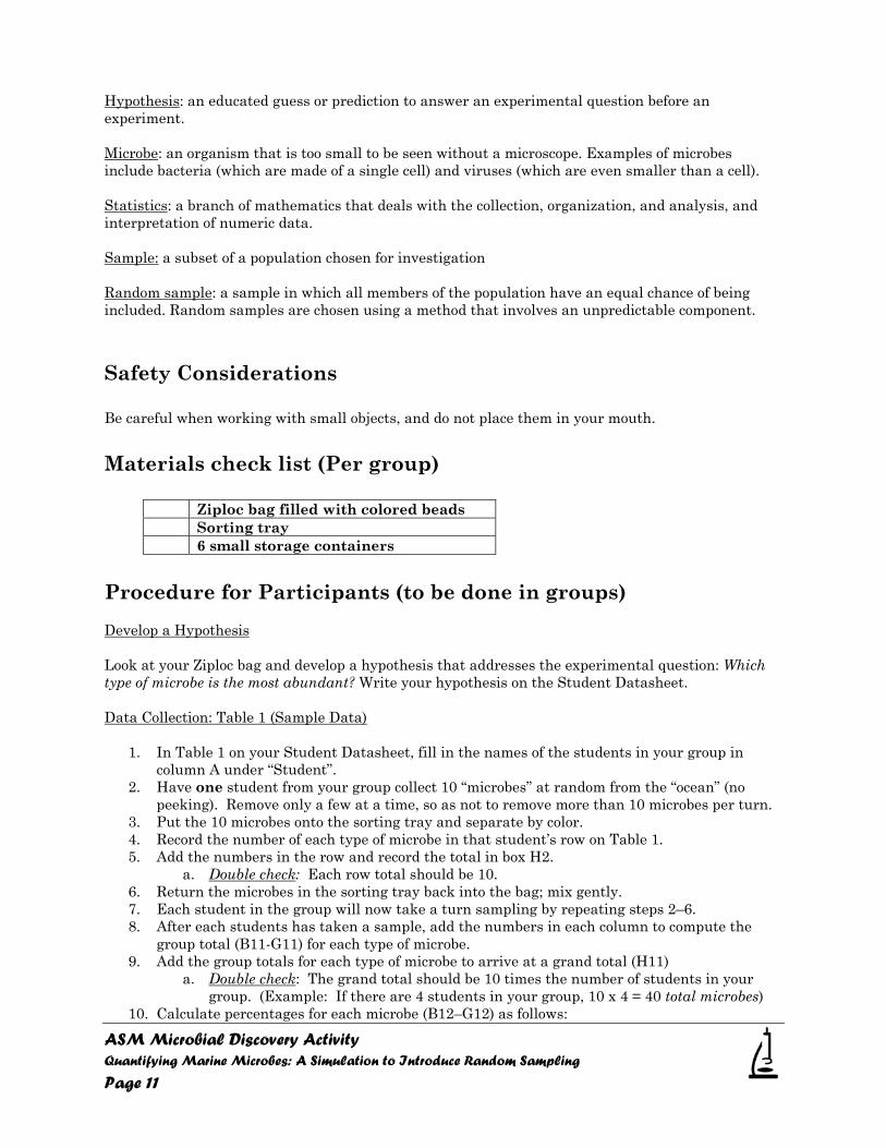
Materials check list (Per group)

Ziploc bag filled with colored beads Sorting tray 6 small storage containers

Procedure for Participants (to be done in groups) Develop a Hypothesis Look at your Ziploc bag and develop a hypothesis that addresses the experimental question: Which type of microbe is the most abundant? Write your hypothesis on the Student Datasheet. Data Collection: Table 1 (Sample Data)

1. In Table 1 on your Student Datasheet, fill in the names of the students in your group in column A under “Student”.

2. Have one student from your group collect 10 “microbes” at random from the “ocean” (no peeking). Remove only a few at a time, so as not to remove more than 10 microbes per turn.

3. Put the 10 microbes onto the sorting tray and separate by color. 4. Record the number of each type of microbe in that student’s row on Table 1. 5. Add the numbers in the row and record the total in box H2.

a. Double check: Each row total should be 10. 6. Return the microbes in the sorting tray back into the bag; mix gently. 7. Each student in the group will now take a turn sampling by repeating steps 2–6. 8. After each students has taken a sample, add the numbers in each column to compute the

group total (B11-G11) for each type of microbe. 9. Add the group totals for each type of microbe to arrive at a grand total (H11)

a. Double check: The grand total should be 10 times the number of students in your group. (Example: If there are 4 students in your group, 10 x 4 = 40 total microbes)

10. Calculate percentages for each microbe (B12–G12) as follows:


Page 12

a. Divide each group total (B11, C11, etc.) by the total number of microbes collected (H11).

b. Multiply by 100% to get percentages. Round to the nearest whole number. Example: If B11 is 4 and H11 is 40, then B12 is 4/40 x 100 = 10%.

c. Double check: Add percentages across row 12 to check that they add up to 100% (within rounding error)

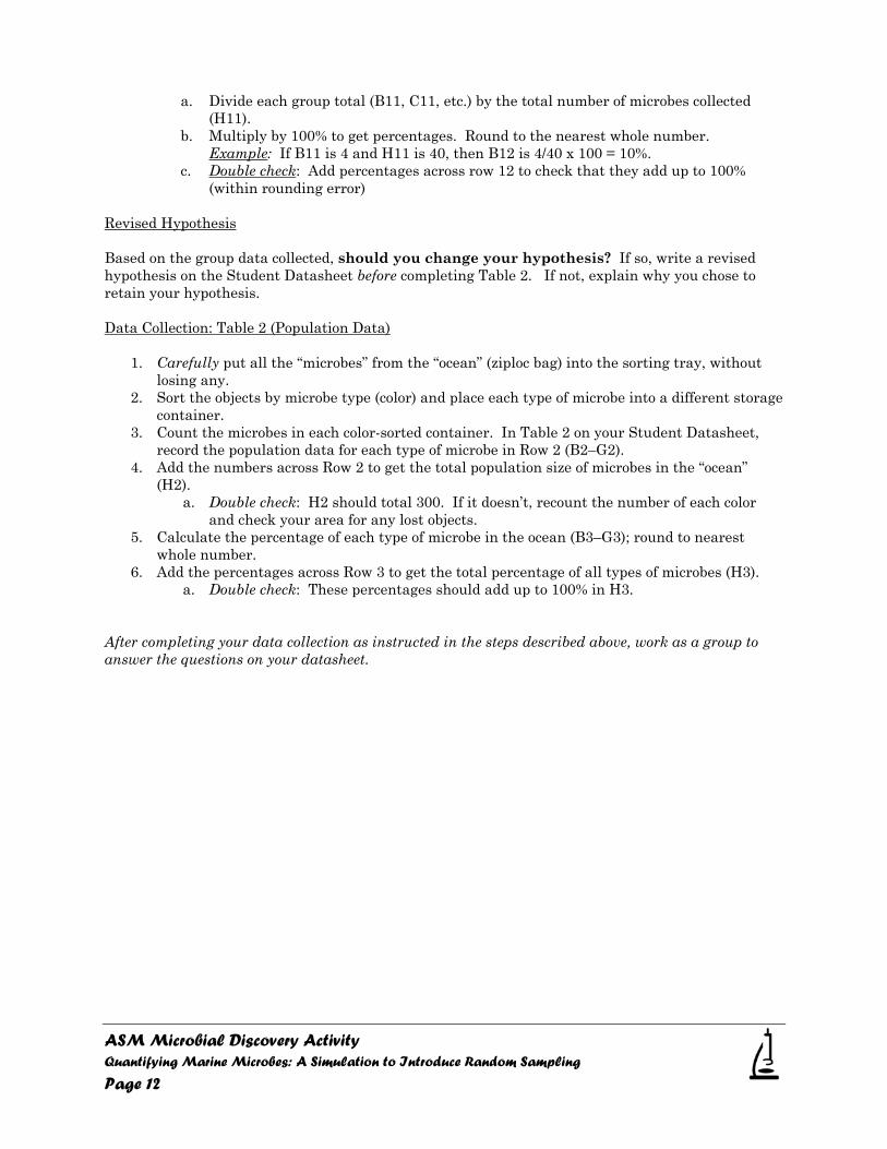
Revised Hypothesis Based on the group data collected, should you change your hypothesis? If so, write a revised hypothesis on the Student Datasheet before completing Table 2. If not, explain why you chose to retain your hypothesis. Data Collection: Table 2 (Population Data)

1. Carefully put all the “microbes” from the “ocean” (ziploc bag) into the sorting tray, without losing any.

2. Sort the objects by microbe type (color) and place each type of microbe into a different storage container.

3. Count the microbes in each color-sorted container. In Table 2 on your Student Datasheet, record the population data for each type of microbe in Row 2 (B2–G2).

4. Add the numbers across Row 2 to get the total population size of microbes in the “ocean” (H2).

a. Double check: H2 should total 300. If it doesn’t, recount the number of each color and check your area for any lost objects.

5. Calculate the percentage of each type of microbe in the ocean (B3–G3); round to nearest whole number.

6. Add the percentages across Row 3 to get the total percentage of all types of microbes (H3). a. Double check: These percentages should add up to 100% in H3.

After completing your data collection as instructed in the steps described above, work as a group to answer the questions on your datasheet.


Page 13

SSStttuuudddeeennnttt WWWooorrrkkkssshhheeeeeettt QQQuuuaaannntttiiifffyyyiiinnnggg MMMaaarrriiinnneee MMMiiicccrrrooobbbeeesss::: AAA SSSiiimmmuuulllaaatttiiiooonnn tttooo IIInnntttrrroooddduuuccceee


Student’s Name __________________________________ Date______________

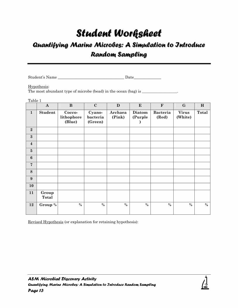
Hypothesis: The most abundant type of microbe (bead) in the ocean (bag) is __________________. Table 1

A B C D E F G H

1 Student Cocco-lithophore

(Blue)


Archaea (Pink)

Diatom (Purple

)

Bacteria (Red)

Virus (White)

Total

2

3

4

5

6

7

8

9

10

11 Group Total

12 Group % % % % % % % %

Revised Hypothesis (or explanation for retaining hypothesis):


Page 14

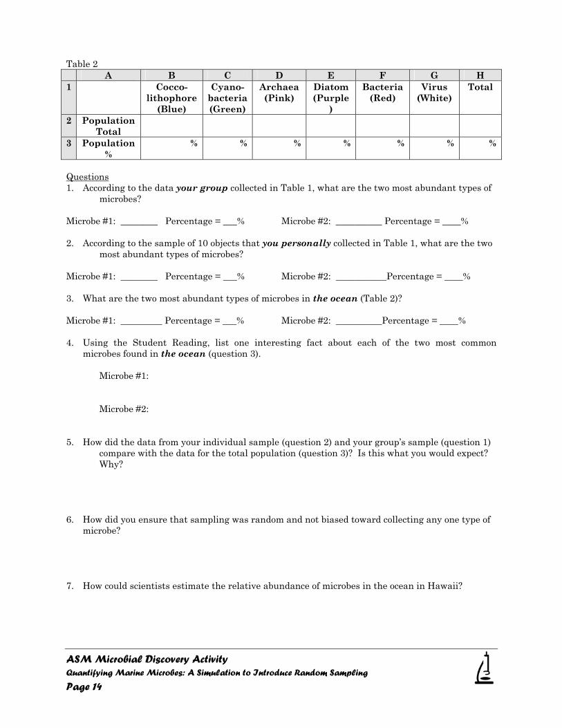
Table 2 A B C D E F G H 1 Cocco-

lithophore (Blue)


Archaea (Pink)

Diatom (Purple

)

Bacteria (Red)

Virus (White)

Total

2 Population Total

3 Population %

% % % % % % %

Questions 1. According to the data your group collected in Table 1, what are the two most abundant types of

microbes?

Microbe #1: ________ Percentage = ___% Microbe #2: __________ Percentage = ____% 2. According to the sample of 10 objects that you personally collected in Table 1, what are the two

most abundant types of microbes?

Microbe #1: ________ Percentage = ___% Microbe #2: ___________Percentage = ____% 3. What are the two most abundant types of microbes in the ocean (Table 2)?

Microbe #1: _________ Percentage = ___% Microbe #2: __________Percentage = ____% 4. Using the Student Reading, list one interesting fact about each of the two most common

microbes found in the ocean (question 3).

Microbe #1: Microbe #2:

5. How did the data from your individual sample (question 2) and your group’s sample (question 1)

compare with the data for the total population (question 3)? Is this what you would expect? Why?

6. How did you ensure that sampling was random and not biased toward collecting any one type of

microbe? 7. How could scientists estimate the relative abundance of microbes in the ocean in Hawaii?


Page 15

SSStttuuudddeeennnttt RRReeeaaadddiiinnnggg::: AAAnnn IIInnntttrrroooddduuuccctttiiiooonnn tttooo MMMaaarrriiinnneee MMMiiicccrrrooobbbeeesss

(((bbbaaassseeeddd ooonnn CCC---MMMOOORRREEE,,, 222000000888 [[[111]]]))) Microbes dominate our planet, especially our oceans. The distinguishing feature of microorganisms is their small size, usually defined as less than 100 micrometers (µm); they are invisible to the naked eye. The similarity among microbes may end there. As a group, marine microbes are extremely diverse. Microbes are found in every ocean environment imaginable. For example, some microbes live near hydrothermal vents[2]; others live inside the tissues of other animals (such as corals and clams); still others live in the ice of Antarctica[3]. Microbes are the most abundant and diverse organisms in the ocean[4]. Just imagine – there are more microbes in the ocean than stars in the known universe! Even more surprising, microbes represent approximately 98% of the ocean’s biomass[5]. This means that if you were to add up the weights of all the whales, sharks, other fish, crustaceans, and all other visible marine life, their combined weight would be only 2% of the total weight of all marine life. This is a good thing because we cannot live without microbes. They form the base of the food web, they are our planet’s principal decomposers, and they produce much of the oxygen that we need to live. Marine microbes were the first life forms, and they enable all other organisms to survive[6]. Thousands of different species of microbes have been identified, and the total keeps growing as new species are continually being discovered[7]. Currently, we recognize three major groups of life on Earth: Archaea, Bacteria, and Eukaryotes. Archaea and bacteria are single-celled organisms that come in a variety of shapes and sizes. They are prokaryotes – that is, they lack a nucleus[8]. All remaining unicellular organisms and all visible forms of life are called Eukaryotes—that is, organisms with nuclei[8]. Viruses are also microbes. However, because they can’t reproduce and grow independently, they are not considered to be alive [9]. The following examples illustrate some of the amazing marine microbes found in each of these groups.

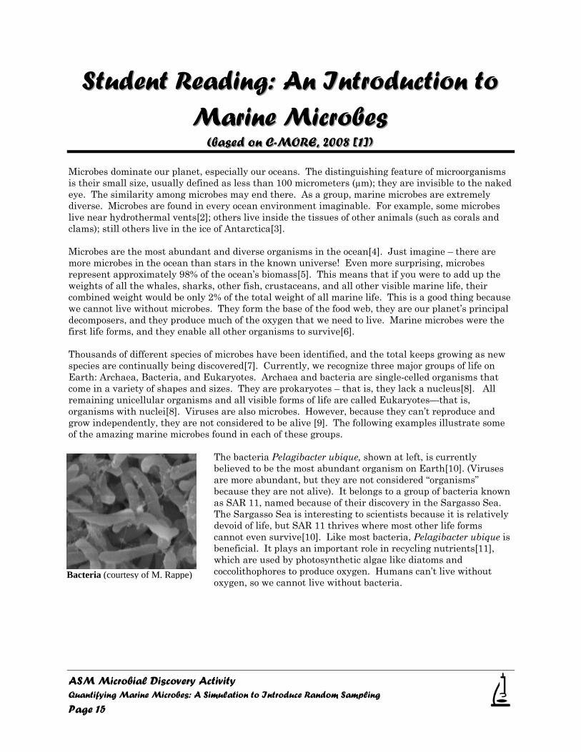
The bacteria Pelagibacter ubique, shown at left, is currently believed to be the most abundant organism on Earth[10]. (Viruses are more abundant, but they are not considered “organisms” because they are not alive). It belongs to a group of bacteria known as SAR 11, named because of their discovery in the Sargasso Sea. The Sargasso Sea is interesting to scientists because it is relatively devoid of life, but SAR 11 thrives where most other life forms cannot even survive[10]. Like most bacteria, Pelagibacter ubique is beneficial. It plays an important role in recycling nutrients[11], which are used by photosynthetic algae like diatoms and coccolithophores to produce oxygen. Humans can’t live without oxygen, so we cannot live without bacteria.

Bacteria (courtesy of M. Rappe)


Page 16

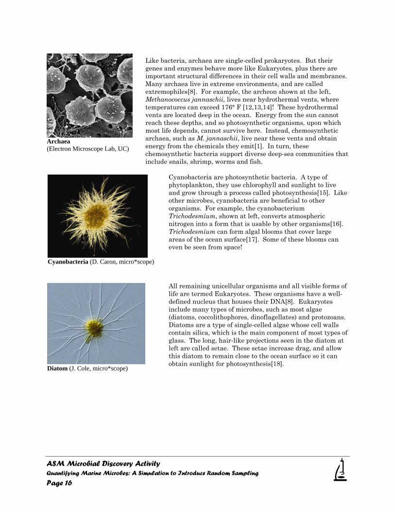
Like bacteria, archaea are single-celled prokaryotes. But their genes and enzymes behave more like Eukaryotes, plus there are important structural differences in their cell walls and membranes. Many archaea live in extreme environments, and are called extremophiles[8]. For example, the archeon shown at the left, Methanococcus jannaschii, lives near hydrothermal vents, where temperatures can exceed 176° F [12,13,14]! These hydrothermal vents are located deep in the ocean. Energy from the sun cannot reach these depths, and so photosynthetic organisms, upon which most life depends, cannot survive here. Instead, chemosynthetic archaea, such as M. jannaschii, live near these vents and obtain energy from the chemicals they emit[1]. In turn, these chemosynthetic bacteria support diverse deep-sea communities that include snails, shrimp, worms and fish.

Cyanobacteria are photosynthetic bacteria. A type of phytoplankton, they use chlorophyll and sunlight to live and grow through a process called photosynthesis[15]. Like other microbes, cyanobacteria are beneficial to other organisms. For example, the cyanobacterium Trichodesmium, shown at left, converts atmospheric nitrogen into a form that is usable by other organisms[16]. Trichodesmium can form algal blooms that cover large areas of the ocean surface[17]. Some of these blooms can even be seen from space! All remaining unicellular organisms and all visible forms of life are termed Eukaryotes. These organisms have a well-defined nucleus that houses their DNA[8]. Eukaryotes include many types of microbes, such as most algae (diatoms, coccolithophores, dinoflagellates) and protozoans. Diatoms are a type of single-celled algae whose cell walls contain silica, which is the main component of most types of glass. The long, hair-like projections seen in the diatom at left are called setae. These setae increase drag, and allow this diatom to remain close to the ocean surface so it can obtain sunlight for photosynthesis[18].

Archaea (Electron Microscope Lab, UC)

Cyanobacteria (D. Caron, micro*scope)

Diatom (J. Cole, micro*scope)


Page 17

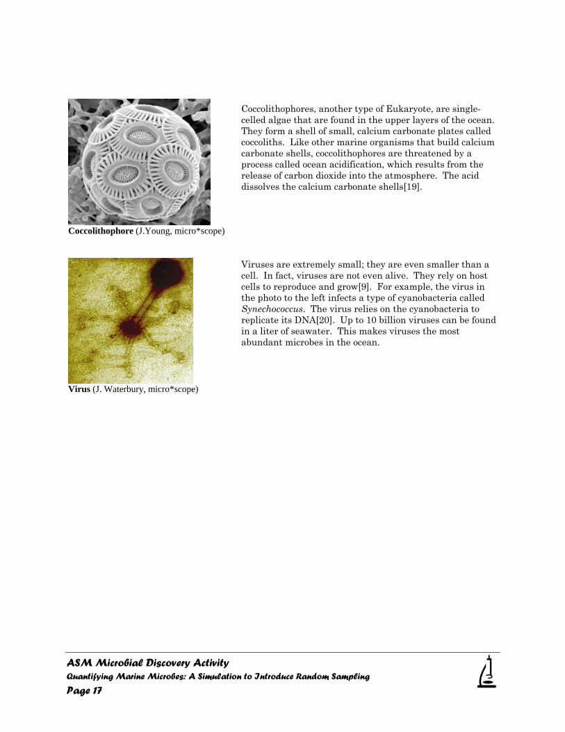
Coccolithophores, another type of Eukaryote, are single-celled algae that are found in the upper layers of the ocean. They form a shell of small, calcium carbonate plates called coccoliths. Like other marine organisms that build calcium carbonate shells, coccolithophores are threatened by a process called ocean acidification, which results from the release of carbon dioxide into the atmosphere. The acid dissolves the calcium carbonate shells[19]. Viruses are extremely small; they are even smaller than a cell. In fact, viruses are not even alive. They rely on host cells to reproduce and grow[9]. For example, the virus in the photo to the left infects a type of cyanobacteria called Synechococcus. The virus relies on the cyanobacteria to replicate its DNA[20]. Up to 10 billion viruses can be found in a liter of seawater. This makes viruses the most abundant microbes in the ocean.

Coccolithophore (J.Young, micro*scope)

Virus (J. Waterbury, micro*scope)


Page 18

Acknowledgements This project was funded by C-MORE (NSF-OIA Award #EF-0424599, D. Karl, PI). Field-testing occurred through C-MORE and Ocean FEST (NSF/OEDG grant #091431, B. Bruno, PI) in partnership with numerous teachers in the Hawaii Department of Education. Many, many educators both within and outside C-MORE contributed to the development, evaluation and field-testing of this activity, particularly K. Weersing, B. Mayer, and S. Sherman. M. Hsia assisted with manuscript preparation. Images were provided by Micro*scope, the Electron Microscope Lab at UC Berkeley, J. Cole, D. Caron, M. Rappe, J. Waterbury, and J. Young. K. Picardo and one anonymous reviewer provided constructive reviews which resulted in a greatly improved manuscript.

References Cited

1. Center for Microbial Oceanography: Research and Education (2008) Key Concepts in Microbial Oceanography. http://cmore.soest.hawaii.edu/downloads/MO_key_concepts_hi-res.pdf

2. Miller, J.F., N.N. Shah, C.M. Nelson, J.M. Ludlow, and D.S. Clark (1988) Pressure and

temperature effects on growth and methane production of the extreme thermophile Methanococcus jannaschii. Applied and Environmental Microbiology 54(12):3039-3042.

3. Price, P.B. (1999) A habitat for psychrophiles in deep Antarctic ice. Proceedings of the National Academy of Sciences 97(3):1247-1251.

4. Sogin, M.L., H.G. Morrison, J.A. Huber, D.M. Welch, S.M. Huse, P.R. Neal, J.M. Arrieta, and G.J. Herndl (2006) Microbial diversity in the deep sea and the underexplored “rare biosphere”. Proceedings of the National Academy of Sciences 103(32):12115-12120.

5. Whitman, W.B., D.C. Coleman, and W.J. Wiebe (1998) Prokaryotes: The unseen majority. Proceedings of the National Academy of Sciences 95:6578-6583.

6. Dolan, John (Lead Author); Jean-Pierre Gattuso (Topic Editor). 2009. "Marine microbes." In: Encyclopedia of Earth. Eds. Cutler J. Cleveland (Washington, D.C.: Environmental Information Coalition, National Council for Science and the Environment). [First published in the Encyclopedia of Earth October 30, 2006; Last revised June 30, 2009; Retrieved March 4, 2010]. <http://www.eoearth.org/article/Marine_microbes>

7. Pomeroy, L.R., P.J.I. Williams, F. Azam, and J.E. Hobbie (2007) The microbial loop. Oceanography 20(2):28-33.

8. "archaea." Encyclopædia Britannica. 2010. Encyclopædia Britannica Online. 04 Mar. 2010

<http://www.britannica.com/EBchecked/topic/32547/archaea>.

9. "virus." Encyclopædia Britannica. 2010. Encyclopædia Britannica Online. 04 Mar. 2010 <http://www.britannica.com/EBchecked/topic/630244/virus>.


Page 19

10. Morris, R. M., M.S. Rappé, S.A. Connon, K.L. Vergin, W.A. Siebold, C.A. Carlson, and S.J. Giovannoni (2002) SAR11 clade dominates ocean surface bacterioplankton communities. Nature 420:806-810.

11. Sowell, S.M., A.D. Norbeck, M.S. Lipton, C.D. Nicora, S.J. Callister, R.D. Smith, D.F. Barofsky, and S.J. Giovannoni (2008) Proteomic analysis of stationary phase in the marine bacterium “Candidatus Pelagibacter ubique”. Applied and Environmental Microbiology 13:4091-4100.

12. Jones, W.J., J.A. Leigh, F. Mayer, C.R. Woese, R.S. Wolfe (1983) Methanococcus jannaschii sp. nov., an extremely thermophilic methanogen from a submarine hydrothermal vent. Archives of Microbiology 136:254-261.

13. Brock, T.D. (1985) Life at high temperatures. Science 230:132-138.

14. Jannasch, H.W. and M.J. Mottl (1985) Geomicrobiology of deep-sea hydrothermal vents. Science 229:717-725.

15. "blue-green algae." Encyclopædia Britannica. 2010. Encyclopædia Britannica Online. 04 Mar. 2010 <http://www.britannica.com/EBchecked/topic/70231/blue-green-algae>.

16. Capone, D.G., J.P. Zehr, H.W. Paerl, B. Bergman, E.J. Carpenter (1997) Trichodesmium, a globally significant marine cyanobacterium. Science 276:1221-1229.

17. Sieburth, J.M. and J.T. Conover (1965) Slicks associated with Trichodesmium Blooms in the Sargasso Sea. Nature 205:830-831.

18. Gebeshuber, I.C. and R.M. Crawford (2006) Micromechanics in biogenic hydrated silica: hinges and interlocking devices in diatoms. Proceedings of the Institution of Mechanical Engineers 220(J):787-796.

19. Doney, S.C., W.M. Balch, V.J. Fabry, and R.A. Feely (2009) Ocean acidification: A critical emerging problem for the ocean sciences. Oceanography 22(4):16-25.

20. Benson, R. and E. Martin (1981) Effects of photosynthetic inhibitors and light-dark regimes on the replication of cyanophage SM-2. Archives of Microbiology 129:165-167.

Documents

Quantifying Marine Microbes: A Simulation to …cmore.soest.hawaii.edu/downloads/2010_quantifying_random...Marine microbes are extremely abundant organisms; a single liter of sea water