Quantifying Poetic Style: A Machine Learning-Based Approach to Poem/Poet Identification

Abstract

Writers are often viewed as having a particular style, unique to their writing. Much work

has been done historically within the field of stylometry in attempting to quantify this literary style. This paper, focusing specifically on the realm of poetry, explores new quantitative features that one might use for this task, specifically in extending existing approaches to include not only the “unconscious” characteristics of literary works, but “conscious” aspects as well. The paper proposes a novel mechanism by which thematic content might be quantified, combining the Word2vec infrastructure with the K-Means Clustering algorithm. The paper explores machine learning classification techniques that might then be used on extracted features to create classifiers that identify the author of poems, and discusses the results of these classification techniques in light of literary understandings of the poets and their poems.

1

1: Introduction

It is generally accepted that authors have unique, inherent, and often recognizable styles of writing. Such an assumption is the foundation of practically every act of literary analysis, which is fundamentally predicated on a belief in authorial style as a distinct and important—and hence, analyzable—characteristic of written work. Because style, under this assumption, serves as a “fingerprint” or “signature” of the author, one should in principle be able to determine the authorship of a written work by simply analyzing the style of the text—and indeed, such a task of authorial identification is prevalent in undergraduate English curricula everywhere (see, for example, the GRE Subject Test in English Literature, required for application to most graduate programs in English and heavily focused upon this precise task). In practice, the difficulty of the task lies primarily in determining precisely what characterizes the style of a particular author—that is, determining which features of the text most accurately summarize an author’s style. When one views this task more specifically in quantitative or statistical terms, the problem is then finding adequate numerical representations of an author’s style.

There has been much work done historically in this field, known as “stylometry”: the statistical analysis of literary style. For a comprehensive review, see Holmes (1985). Early attempts to quantify style relied primarily on word frequency counts or word length counts. The most significant early example is that of Mendenhall, who described the word length distributions of Shakespeare and Bacon and, from a consideration of the differing shapes of these so-called “characteristic curves” (namely, from the fact that the most frequent word length of Shakespeare was four, while that of Bacon was three), concluded that it was unlikely that Bacon wrote any of Shakespeare’s disputed works (1901). Brinegar similarly constructed a characteristic curve for Mark Twain to determine whether he had written the Quintus Curtius Snodgrass letters; taking a more rigorous statistical approach than Mendenhall, Brinegar then employed a Chi-Squared goodness of fit test and a two-sample t-tests on the counts of two-, three-, and four-letter words to conclude that the letters were not written by Twain (1963).

Fucks, in a work on various English and German authors, calculated the average number of syllables per word as well as the relative frequencies of i-syllabled words and their distribution in the text (1952); in a later study with Lauter, he discovered that frequency distributions of syllables per word discriminated different languages more effectively than specific authors (1965).

Yule took a higher-level approach, zooming out from syllables and words and instead using sentence length to determine authorship for The Imitation of Christ, though he ultimately concluded that sentence-length statistics were not a wholly reliable indicator (1938). Williams repeated this sentence-length approach on works written by Chesterton, Wells, and Shaw; he discovered that the frequency distribution of the logarithm of the number of words per sentence was approximately Normal (1940). Such an approach was similarly implemented by Morton, who analyzed ancient Greek texts (1965).

Mosteller and Wallace, initially following two of the above methods, considered criteria such as word length and sentence length in their analysis of the Federalist Papers. They found, however, little difference between Madison and Hamilton with respect to these features (1963). They then turned their focus to counts of function words: words with little contextual meaning that are used almost unconsciously (examples include of, the, that, and, or) (1964). Through a

2

consideration of the frequency distributions of a few function words, modeled by the negative binomial distribution (which they determined to be a better fit for the data than the Poisson distribution because of its heavier tail), they successfully assigned authorship to the unsigned Federalist Papers in what is widely considered the first convincing demonstration of the power of quantitatively analysis in determining textual authorship.

Antosch turned instead to consider the distribution of different parts of speech (that is, the different percentages of nouns, verbs, adjectives, adverbs, and other parts of speech in a text); he focused specifically on the verb-adjective ratio for various literary genres and showed that the ratio was highly dependent on the theme of the work, with folk tales having high values and scientific works low (1969). Brainerd built upon this work, considering the usage of articles and pronouns in particular in novels and romances; he concluded that novels tend to give higher pronoun counts and smaller article counts than romances do (1973).

Research within the realm of quantifying authorial style, as such, has largely focused upon the use of stylistic features that are considered “unconscious” on the part of the author (length of words used, number of syllables per word, use of function words, distribution of parts of speech), demonstrating a significant bias against more “conscious” aspects of style. This bias is stated most explicitly by Bailey, who wrote that features considered as candidates for quantitatively summarizing authorial style should “be salient, structural, frequent and relatively immune from conscious control” (1979). Underlying this approach is a narrow definition of style as that which is simply an innate—not consciously chosen—attribute of the author’s writing. As a result, little work has been done on the aspects of style that might be considered more consciously chosen on part of the author: the sentimental valence of meaningful word choice, the overall thematic content of the work. But such aspects, one might argue, are indeed significant—if not the most significant—components of style if one correctly broadens its definition. That which the author has actual control over and chooses consciously is, in a sense, that which the author himself determines to be his style, or how the author himself wishes to characterize his own work. The bulk of the task of the writer stems from authorial choice. The conscious aspects of style are hence not a factor to be avoided, but a factor to be considered: an essential component of what makes the author himself. This lack of work on the conscious aspects of style is not the only deficiency that plagues the field of stylometry: work within the field has historically used rather rudimentary methods of statistical analysis such a simple hypothesis testing, as mentioned above. With the modernization of computational abilities, more recent work on this problem of quantifying authorial style has turned to considering each text as a collection of multivariate observations and hence, employed more sophisticated multivariate statistical methods. As examples: Holmes used hierarchical cluster analysis on measures of richness of vocabulary to detect changes in authorship of The Book of Mormon (1992); Peng and Hengartner more recently used canonical discrimination analysis and principal component analysis on function word counts to determine authorship among a set of novelists including Jane Austen, Arthur Conan Doyle, Charles Dickens, Rudyard Kipling, and Jack London (2002); Binongo similarly used principal component analysis on function word counts to determine authorship of The Fifteenth Book of Oz (2003), an approach that was again used by Dabagh in discriminating between different Persian authors (2007). Nevertheless, work in stylometry has failed to take advantage of more complex machine learning techniques now available at our disposal. This paper, then, aspires to remedy these two apparent gaps in our understanding of quantitative representations of authorial style: firstly, by extracting not only the unconscious

3

features of style, but the conscious as well; and secondly, by implementing more sophisticated machine learning algorithms in developing models of style based on these extracted features. The approach taken, furthermore, will consider poems rather than works written in prose, another historical gap in the field of stylometry, and hence examine features relevant to poetry that do not arise in prose (number of words per poetic line, for example, a feature that becomes particularly emblematic of conscious authorial style in free verse, where the poet must decide where a line break occurs). The paper considers the body of work of eight poets (Shakespeare, John Milton, William Wordsworth, John Keats, Robert Browning, William Butler Yeats, Walt Whitman, Emily Dickinson) that span a variety of time periods (from Elizabethan to Modern) and geographic locations (England and the United States). It employs the use of multiple machine learning techniques, including Support Vector Machines (with linear, polynomial, and radial kernels), multinomial logistic regression (both with and without the shrinkage methods of LASSO and ridge), K-Nearest Neighbors, and random forests; all of these techniques are commonly employed in classification tasks, and most have the advantage of determining features of importance or delineating how each feature contributes to the classification (as opposed to neural networks, for instance, which are more of a “black box” method). This is significant, because the project—to create a classifier that successfully learns the characteristics of certain poets and applies what it has learned to correctly pair poems with their appropriate poet—aims not at determining authorship in a case where authorship is unclear/disputed, but at revealing something fundamental about what features of an individual poem most characterizes the style of its poet, attempting to replicate that which goes through the mind of an undergraduate English major who is given a poem and asked to identify its author. It aims, furthermore, at an examination of how stylistic difference reveals a historical chain of poetic influence. The project, then, addresses the following questions: What are the most important features that differentiate the style of one poet from another? Which poems are most often misidentified? Which poet is most often misidentified? For whom are they most often confused? Why?

2: Methodology

2.1: Data

I summarize the implementation of the task as essentially a two-step process: first, extracting a set of features that we have deemed important from the set of poems by the poets under consideration; second, feeding these extracted features into various classifiers to test their viability as predictors through their performances in the identification task. I will call the first step “feature extraction,” and the second “model building.”

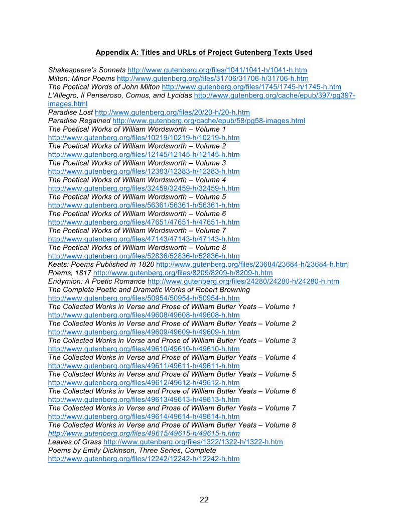
The raw data for this project was obtained from Project Gutenberg, where multiple books of poems by each author were downloaded in text format and processed to separate individual poems and remove editorial characteristics such as word glosses or editor’s footnotes. The titles and URLs for these texts are listed in Appendix A. The raw data includes 983 poems, with over 100 poems by each of eight poets (excepting Keats, for whom I have 91 poems); this is found in the file master.csv. I randomize the ordering of these poems, and separate them into a training set (80 percent of the poems) and a test set (20 percent of the poems). With this training set of raw data (that is, poems) in hand, I proceed to the feature extraction step. 2.2: Feature Extraction

The features extracted for each of the 983 poems can be separated into two broad categories: the technical (that is, the features that describe formal characteristics of the poem); and the thematic (that is, the features that describe the content of the poem). I detail first the technical

4

features and the methods by which they were extracted. Tokenization of the poems for these features is done by the word_tokenize function, and part-of-speech tagging is performed by the pos_tag function using the universal tagset. Both functions are a part of the Python package nltk. The extracted technical features are: num_lines: the number of poetic lines in the poem, where each new line is denoted by a line break in the poem avg_words_per_line: the average number of words per line in the poem, calculated by dividing the number of words in the poem by the number of lines in the poem num_words: the number of words in the poem, where each new word is denoted by a white space in the poem verb: the percentage of tokens in the poem that are tagged as verbs noun: the percentage of tokens in the poem that are tagged as nouns pron: the percentage of tokens in the poem that are tagged as pronouns adj: the percentage of tokens in the poem that are tagged as adjectives adv: the percentage of tokens in the poem that are tagged as adverbs adp: the percentage of tokens in the poem that are tagged as adpositions conj: the percentage of tokens in the poem that are tagged as conjunctions det: the percentage of tokens in the poem that are tagged as determiners prt: the percentage of tokens in the poem that are tagged as participles punctuation: the percentage of tokens in the poem that are tagged as punctuation marks Note also that the pos_tag function output includes a category for words that it does not recognize, so that verb + noun + pron + adj + adv + adp + conj + det + prt + punctuation for a given poem may not precisely equal 1; I choose to leave out this additional category so that the chosen part-of-speech features remain linearly independent. I now proceed with the thematic features, which present a more difficult problem. I first use the established method of sentiment analysis, as implemented by the SentimentIntensityAnalyzer of the nltk.sentiment.vader package. This gives me the following two features: positive: the average positive polarity score for the words in the poem (the “percentage” of words in the poem that are positive, where each word is weighted by the intensity of its valence) negative: the average negative polarity score for the words in the poem (the “percentage” of words in the poem that are negative, where each word is weighted by the intensity of its valence) Note that the SentimentIntensityAnalyzer output includes also a category for a neutral polarity score, so that positive + negative for a given poem may not precisely equal 1; I choose to leave out this additional category so that the chosen sentiment features remain linearly independent. I want, however, something more complicated than simply measures of overall positivity or negativity of the words used within a poem: I want themes. I consider simply extracting frequency counts for numerous words, but decide against this approach to avoid inducing subjectivity in the choice of what I see to be themes amongst the poems, and to avoid the problem of sparse data. Rather, I implement two more complex methodologies: firstly, the Word2vec/K-Means Clustering Approach, a method newly described in this paper; secondly, the Latent Dirichlet Allocation Approach, an already-established method of topic modeling.

5

2.2.1: Word2vec/K-Means Clustering Approach

The Word2vec/K-Means Clustering approach, as the name suggests, combines the strengths of two already-existing concepts. I will describe each in turn: Word2vec is a class of models that are used to produce word embeddings; it was created by a team of researchers at Google, led by Tomas Mikolov (2013). The models themselves are shallow, two-layer neural networks that are trained to reconstruct the semantic meanings of words. Each model takes as its input a large corpus of text and produces a vector space, where each unique word in the corpus is assigned a corresponding vector in the space. Word vectors are positioned in the vector space such that words that share common contexts (and hence, likely common semantic meanings) are located in close proximity to one another in the space. The canonical example of this is that the following equation, where each word is transformed into a vector in the vector space, roughly holds for a properly trained Word2vec model: king – man + woman = queen. In this project, I use a model made available through the gensim

package, which is trained on GoogleNews articles with a vector space of 300 dimensions. K-Means Clustering is a method of cluster analysis used in data mining. It aims to partition n observations into k clusters S = {S1, S2, …, Sk}, where each observation belongs to the cluster with the nearest mean. It aims to do so by minimizing the within-cluster sum of squares. Formally, the objective function is:

argmin'

( − *+,

-∈'0

1

+23

where *+ is the mean of the points in the cluster Si. The most common algorithm used to solve this objective function is an iterative refinement technique, known as the K-Means Algorithm. It begins with a randomly assigned initial set of k means m1

(1), m2

(1), …, mk

(1), which, under the Forgy method, are k randomly chosen observations from the data set. The algorithm then alternates between two steps: Assignment step: Each observation is assigned to the cluster with the “nearest” mean—that is, the mean with the least squared Euclidean distance from the observation. Update step: The means are “updated” to be the centroids of the observations in the new clusters. The algorithm converges when the k clusters have stabilized – that is, when the observation assignments no longer change. In this project, I use the implementation of the KMeans function from the package sklearn.cluster. The Word2vec/K-Means Clustering Approach combines these two methods. It first gathers all the words that a certain poet uses in his/her poems that are in the training set, excluding any stopwords (as identified by the English stopwords set in the package nltk.corpus) as we are primarily interested in words with semantic meaning/significance; doing so for all eight poets creates eight lists of words, one for each poet. Next, it applies the Word2vec embedding on each of the eight lists, so that each list is transformed from a list of words into a list of 300-dimensional vectors in our Word2vec vector space. It then uses K-Means Clustering on each of these eight vector lists to find k means for each poet—k centroids of meaning that should be semantically close to something like the thematic centers of each poet’s poems. Finally, for

6

each poem in the training and test set, it takes the average Euclidean distance between each word of the poem and each of the 8*k centroids, yielding 8*k extracted features for the poem. Each of these features denotes the “closeness” of that poem to each of the poet’s k centroids and hence, theoretically is a measure of how “similar” the thematic content of the particular poem is to each of the poet’s overall bodies of work. Using this approach, I generate two extracted feature data sets: one with k = 1 centroid per poet, and the other with k = 2 centroids per poet. I choose not to go above k = 2 because I find in the model building step that models with k = 3 and above do not perform with higher accuracy, perhaps as a result of overfitting with too many centroids of meaning per poet (interestingly, this perhaps can be extrapolated to mean that each poet only writes about one or two different “topics” throughout his/her poetic career). 2.2.2: Latent Dirichlet Allocation Approach

Latent Dirichlet Allocation is a statistical model used for topic modeling, as presented by Blei, Ng, and Jordan (2003). It takes as input a set of documents (called the corpus), and processes these documents so as to come up with a list of topics for them. Under the approach, documents are then represented as random mixtures over topics, and each topic is characterized by a distribution over all words. It assumes a sparse Dirichlet prior for the topic distribution, encoding the intuition that documents cover only a small set of topics and that topics use only a small set of words frequently. The generative process for the approach, more formally, is as follows for a corpus D consisting of M documents each of length Ni where K topics are desired: 1. Choose 4+~678 9 , where 7 ∈ 1, … ,= and 678 9 is a Dirichlet distribution with a sparse

symmetric parameter 9 (9 < 1). 2. Choose A1~678(C), where D ∈ 1, … , E and C is sparse 3. For each of the word positions i, j where 7 ∈ 1, … ,= and F ∈ 1, … , G :

a. Choose a topic I+,J~KLMNOP87QLR(4+)

b. Choose a word S+,J~KLMNOP87QLR AT0,U

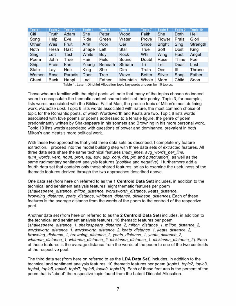
In the specific case of this project, the observations (or documents) are poems. The poems of the training set are placed together into a corpus, which goes through a number of pre-processing steps (including: removing punctuation, stripping digits, removing stopwords, stripping whitespace, stemming to ensure that different verb forms of the same word aren’t duplicated, transforming to lower case, and removing outlying words that are too rare or outlying documents that have no popular words). Our corpus then generates a list of K topics for the poems, which are used to characterize each poem as a mixture of these topics. This approach yields K extracted for each poem, where each of the K features is a “percentage” of how much of the poem is “about” that topic. I use the implementation of the tm, topicmodels, and SnowballC packages. With this approach, I generate an additional extracted feature data set. I use K = 10. I choose K = 10 on the basis of viewing lists of topic keywords generated by different values of K, where I believe K = 10 to be the maximum number of topics where each topic is still distinct and coherent. With K = 10 on one randomly selected training set, the Latent Dirichlet Allocation approach generates 10 topics with the following keywords:

7

Topic 1 Topic 2 Topic 3 Topic 4 Topic 5 Topic 6 Topic 7 Topic 8 Topic 9 Topic 10

Citi Truth Adam She Peter Wood Faith She Doth Hell Song Help Eve Ride Green Water Prove Flower Prais Glori Other Was Fruit Arm Poor Oer Since Bright Sing Strength Noth Flesh Hast Shape Left Star True Soft Dost King Sing Left Tast White Boy Rock Whi Wing Hast Angel Poem John Tree Hair Field Sound Doubt Rose Thine Foe Ship Prais Farr Young Beneath Stream Tri Tell Dear Lost State Lay Hee King She Dim Truth Oer Ill Throne Women Rose Paradis Door Tree Wave Better Silver Song Father Chant Back Happi Ladi Father Mountain Whole Morn Child Soon

Table 1: Latent Dirichlet Allocation topic keywords chosen for 10 topics.

Those who are familiar with the eight poets will note that many of the topics chosen do indeed seem to encapsulate the thematic content characteristic of their poetry. Topic 3, for example, lists words associated with the Biblical Fall of Man, the precise topic of Milton’s most defining work, Paradise Lost. Topic 6 lists words associated with nature, the most common choice of topic for the Romantic poets, of which Wordsworth and Keats are two. Topic 8 lists words associated with love poems or poems addressed to a female figure, the genre of poem predominantly written by Shakespeare in his sonnets and Browning in his more personal work. Topic 10 lists words associated with questions of power and dominance, prevalent in both Milton’s and Yeats’s more political work.

With these two approaches that yield three data sets as described, I complete my feature extraction. I proceed into the model building step with three data sets of extracted features. All three data sets share the same technical features (num_lines, avg_words_per_line, num_words, verb, noun, pron, adj, adv, adp, conj, det, prt, and punctuation), as well as the same rudimentary sentiment analysis features (positive and negative). I furthermore add a fourth data set that contains only these shared features, so as to examine the usefulness of the thematic features derived through the two approaches described above.

One data set (from here on referred to as the 1 Centroid Data Set) includes, in addition to the technical and sentiment analysis features, eight thematic features per poem (shakespeare_distance, milton_distance, wordsworth_distance, keats_distance, browning_distance, yeats_distance, whitman_distance, dickinson_distance). Each of these features is the average distance from the words of the poem to the centroid of the respective poet.

Another data set (from here on referred to as the 2 Centroid Data Set) includes, in addition to the technical and sentiment analysis features, 16 thematic features per poem (shakespeare_distance_1, shakespeare_distance_2, milton_distance_1, milton_distance_2, wordsworth_distance_1, wordsworth_distance_2, keats_distance_1, keats_distance_2, browning_distance_1, browning_distance_2, yeats_distance_1, yeats_distance_2, whitman_distance_1, whitman_distance_2, dickinson_distance_1, dickinson_distance_2). Each of these features is the average distance from the words of the poem to one of the two centroids of the respective poet.

The third data set (from here on referred to as the LDA Data Set) includes, in addition to the technical and sentiment analysis features, 10 thematic features per poem (topic1, topic2, topic3, topic4, topic5, topic6, topic7, topic8, topic9, topic10). Each of these features is the percent of the poem that is “about” the respective topic found from the Latent Dirichlet Allocation.

8

The last data set (from here on referred to as the Non-Thematic Data Set) includes only the technical and sentiment analysis features. 2.3: Model Building

The model building step of my method takes in the extracted features (in all four data sets), feeding them into various classifiers to test their viability as predictors. This is done by measuring their performance in an identification task with the test set of poems. The same models are used for each of the four data sets so that direct comparison may follow. I now detail the classifiers used and their respective implementations. I choose not to go into tremendous theoretical detail, as the methods here used are well-established and well-understood within the field of machine learning. 2.3.1: Support Vector Machines

Support vector machines (SVMs) are supervised learning models. I will here describe an SVM model where there are only two classes of the response variable for mathematical clarity, noting that my model requires an extension of this (as there are eight classes of the response variable, the poets). In the case of my multiclass model, the one-versus-one approach is implemented: V, SVMs are trained (one for each possible pairing of the eight classes), and labels on the test

set are determined by “vote” (which label is most frequently classified in all of the SVM models). With a linear kernel and two response variable classes, the SVM is a binary linear classifier. It takes in each data point of the training set as a p-dimensional vector and constructs a single hyperplane in the p-dimensional space to separate these data points based on the response variable (in this case, the poet). This hyperplane is a flat affine subspace of dimension p-1, of the form:

CW +C3Y3 + ⋯+C[Y[ = 0

A separating hyperplane is that which can perfectly divide the classes we are predicting—that is, a hyperplane where for each response ^+ ∈ −1, 1 , ∃CW, … , C[such that

^+ CW + C3(+3 + ⋯+C[(+[ > 0 If a single separating hyperplane exists, infinite separating hyperplanes exist. The best separation, then, is determined by the hyperplane that has the largest functional margin—that is, the largest distance to the nearest training-data point of any class; this best separating hyperplane is known as the maximal margin hyperplane. Support vectors are the vectors drawn from the training observations closest to the maximal margin hyperplane to the hyperplane itself. Because the maximal margin hyperplane is hence dependent on a calculation of Euclidean distance, it is important that the data be scaled. A larger functional margin generally results in higher certainty in predicted class and hence lower generalization error for the classifier. The maximal margin hyperplane, then, solves the following maximization problem:

maxbc,…,bd

= such that CJ, = 1[

J23 , where ^+(CW + C3(+3 + ⋯+C[(+[) ≥ = for all i = 1, …,n

In many cases, however, no perfect separating hyperplane exists, such that for any choice of CW, … , C[, there exists at least one observation i such that ^+ CW + C3(+3 + ⋯+C[(+[ < 0. In

9

this case, we seek a soft margin that performs the best at almost separating the classes. The new maximization problem in this case is to maximize M with by choosing CJ and f+ such that

^+(CW + C3(+3 + ⋯+C[(+[) ≥ =(1 − f+)

where CJ, = 1[

J23 , f+ ≥ 0, f+g+23 ≤ K. The f+ are slack variables that indicate which side of the

margin or hyperplane the observation is on, and C is a cost variable that determines by how much the margin can be violated (it constrains the model to having no more than C observations on the wrong side of the hyperplane). In this case, observations directly on the margin or on the wrong side of the margin are the support vectors. Hence, a larger C yields more support vectors, but also a more robust classifier. In addition to the linear classification described above, SVM can also efficiently perform non-linear classification by using the kernel trick. The algorithm is formally similar, except that every dot product is replaced by a nonlinear kernel function, which allows the maximum-margin hyperplane to be fit in a transformed, usually high-dimensional feature space. Rather than the traditional dot product kernel function used in linear classification (E (+, (

i+ =< (+, (′+ >), SVM

can employ nonlinear kernel functions such as the polynomial kernel of degree d > 1 (note that a polynomial kernel of degree 1 is equivalent to a translated linear kernel):

E (+, (i+ = (1+< (+, (

i+ >)

k

and the radial kernel with l > 0, where l determines the variance of the Gaussian:

E (+, (i+ = exp(−l ((+J − (

i+J)

,)

[

J23

Because all four of my data sets are high-dimensional, it is difficult to tell a priori which kernel function is best suited to the data. Hence, I choose to try each in turn. I implement a linear kernel, polynomial kernel, and radial kernel SVM. These are all done using the e1071 package, where scaling of the data is built in. Linear Kernel: I use the tune function to choose an appropriate value of cost C from 0.001, 0.01, 0.1, 1, 10, 20, and 30 by cross-validation on my training set. This results in the following four models: 1 Centroid Data Set: Cost = 20, 350 support vectors 2 Centroid Data Set: Cost = 20, 372 support vectors LDA Data Set: Cost = 10, 328 support vectors Non-Thematic Data Set: Cost = 30, 506 support vectors Polynomial Kernel: I use the tune function to choose an appropriate value of cost C from 0.001, 0.01, 0.1, 1, 10, 20, and 30, as well as an appropriate value of degree d from 2, 3, 4, and 5 by cross-validation on my training set. This results in the following four models: 1 Centroid Data Set: Cost = 30, Degree = 3, 574 support vectors 2 Centroid Data Set: Cost = 20, Degree = 3, 576 support vectors LDA Data Set: Cost = 20, Degree = 3, 516 support vectors Non-Thematic Data Set: Cost = 30, Degree = 3, 636 support vectors

10

Radial Kernel: I use the tune function to choose an appropriate value of cost C from 0.001, 0.01, 0.1, 1, 10, 20, and 30, as well as an appropriate value of gamma from 0.01, 0.1, 0.5, 1, 2, 3, and 4 by cross-validation on my training set. This results in the following four models: 1 Centroid Data Set: Cost = 30, Gamma = 0.01, 566 support vectors 2 Centroid Data Set: Cost = 30, Gamma = 0.01, 558 support vectors LDA Data Set: Cost = 1, Gamma = 0.01, 567 support vectors Non-Thematic Data Set: Cost = 20, Gamma = 0.01, 635 support vectors 2.3.2: Multinomial Logistic Regression

Multinomial logistic regression is a classification method that generalizes logistic regression to multiclass problems (that is, cases where the response variable has more than two possible discrete outcomes). In our case, where we have eight possible outcomes, the multinomial logistic regression can be thought of as seven independent binary logistic regression models, where one outcome is chosen as a “pivot” and the other seven outcomes are separately regressed against the pivot outcome. Suppose without loss of generality that this pivot outcome is “shakespeare.” Then, the model considers the following set of equations:

ln(p(q021)

p(q02irst1ur[utvuw)) = C1 ∗ Y+

where D ∈ y ={ ‘milton’, ‘wordsworth’, ‘keats’, ‘browning’, ‘yeats’, ‘whitman’, ‘dickinson’}. Hence, we now have a separate set of regression coefficients for each possible outcome. Exponentiating both sides and solving for probabilitie gives us:

z {+ = D = z {+ =i |ℎLDN|~NL8Ni Nb�∗Ä0 where D ∈ y

Since all 8 of the probabilities must sum to 1,

z {+ =i |ℎLDN|~NL8Ni = 1 − z {+ = ′|ℎLDN|~NL8N′ Nb�∗Ä0

1∈'

so

z {+ =i |ℎLDN|~NL8Ni =

1

1 + Nb�∗Ä01∈'

From this, we can solve for all of the other probabilities:

z {+ = D = uÅ�∗Ç0

3É uÅ�∗Ç0�∈Ñ where D ∈ y

The unknown parameters in each vector C1 are estimated by maximum likelihood estimation. For each of my data sets, I run a multinomial logistic regression on all predictors. All predictors are found to be significant at an 9 = 0.05 level except for num_words: this makes sense, as it is a redundant variable (since num_words = num_lines * avg_words_per_line). The multinomial logistic regression is implemented by using the multinom function from the nnet package. I choose here to omit the coefficients for these four models, as each model has a large number of coefficients due to the eight classes of the response variable.

11

2.3.3: K-Nearest Neighbors

The K-Nearest Neighbors algorithm (KNN) is a non-parametric method used for classification. It is a type of instance-based learning, where the function is approximated only locally; the algorithm is hence sensitive to the local structure of the data. The input consists of the k closest (by Euclidean distance) training observations in the feature space. Because the method is hence dependent on calculations of Euclidean distance, it is important to scale data for this approach. For a given observation (+ to be classified, the algorithm takes the k nearest neighbors of that observation and gives it the majority label of these k nearest neighbors. More formally, with G+ as the set of k observations closest to (+ in the feature space,

Ü = argmax1∈'

á g = Dg∈à0

where y ={‘shakespeare’, ‘milton’, ‘wordsworth’, ‘keats’, ‘browning’, ‘yeats’, ‘whitman’, ‘dickinson’}.

For each of my four data sets, I implement KNN using the knn function from the FNN package. I split my training set into a training_temp set (80% of the training data) and a validation set (20% of the training data), then scale both of these subsets. I use cross-validation on this training_temp and validation set to choose an appropriate value of k from 1 through 20. This results in the following values of k for each of my data sets: 1 Centroid Data Set: k = 11, k = 17 2 Centroid Data Set: k = 14, k = 19, k = 20 LDA Data Set: k = 16, k = 19 Non-Thematic Data Set: k = 7 2.3.4: Random Forest

Random forests are an ensemble learning method for classification that operate by constructing a multitude of decision trees during training and labeling test data by the class that gathers the most “votes” from these individual trees. Random forests inherently average multiple decision trees, trained on different parts of the same training set, with the goal of correcting the primary weakness of decision trees: overfitting to the training set. This comes at the expense of a small increase in bias and some loss of interpretability, but generally boosts performance in the final model. The training algorithm for random forests applies the technique of bagging (or bootstrap aggregating) to tree learners. Given a training set of observations with their respective responses, bagging repeatedly (B times) selects a random sample with replacement from the

training set and grows a trees using each of these samples, giving us B trees (M(3), … , M â ). After training, the prediction for a given observation (+ can be made by taking the majority vote across the B trees, so that

Ü = M ätã (+ = argmax1∈'

á{M ä (+ = D}

â

ä23

where y ={‘shakespeare’, ‘milton’, ‘wordsworth’, ‘keats’, ‘browning’, ‘yeats’, ‘whitman’, ‘dickinson’}.

12

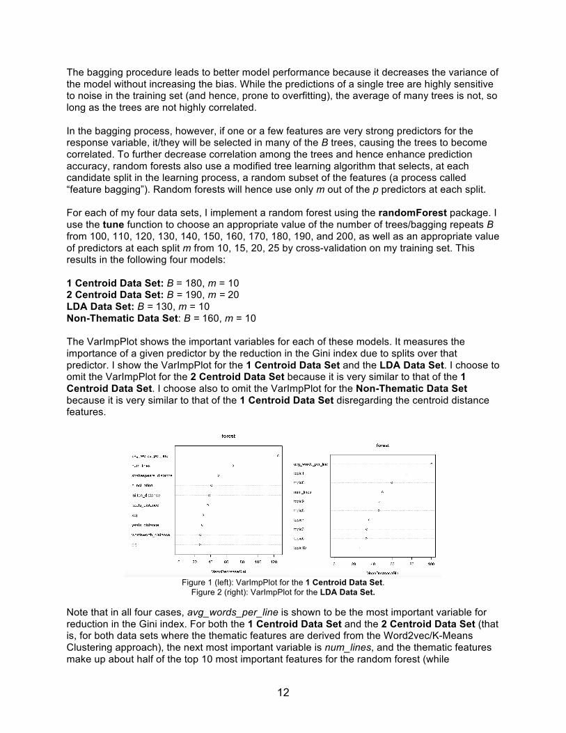
The bagging procedure leads to better model performance because it decreases the variance of the model without increasing the bias. While the predictions of a single tree are highly sensitive to noise in the training set (and hence, prone to overfitting), the average of many trees is not, so long as the trees are not highly correlated. In the bagging process, however, if one or a few features are very strong predictors for the response variable, it/they will be selected in many of the B trees, causing the trees to become correlated. To further decrease correlation among the trees and hence enhance prediction accuracy, random forests also use a modified tree learning algorithm that selects, at each candidate split in the learning process, a random subset of the features (a process called “feature bagging”). Random forests will hence use only m out of the p predictors at each split. For each of my four data sets, I implement a random forest using the randomForest package. I use the tune function to choose an appropriate value of the number of trees/bagging repeats B from 100, 110, 120, 130, 140, 150, 160, 170, 180, 190, and 200, as well as an appropriate value of predictors at each split m from 10, 15, 20, 25 by cross-validation on my training set. This results in the following four models: 1 Centroid Data Set: B = 180, m = 10 2 Centroid Data Set: B = 190, m = 20 LDA Data Set: B = 130, m = 10 Non-Thematic Data Set: B = 160, m = 10 The VarImpPlot shows the important variables for each of these models. It measures the importance of a given predictor by the reduction in the Gini index due to splits over that predictor. I show the VarImpPlot for the 1 Centroid Data Set and the LDA Data Set. I choose to omit the VarImpPlot for the 2 Centroid Data Set because it is very similar to that of the 1

Centroid Data Set. I choose also to omit the VarImpPlot for the Non-Thematic Data Set

because it is very similar to that of the 1 Centroid Data Set disregarding the centroid distance features.

Figure 1 (left): VarImpPlot for the 1 Centroid Data Set.

Figure 2 (right): VarImpPlot for the LDA Data Set.

Note that in all four cases, avg_words_per_line is shown to be the most important variable for reduction in the Gini index. For both the 1 Centroid Data Set and the 2 Centroid Data Set (that is, for both data sets where the thematic features are derived from the Word2vec/K-Means Clustering approach), the next most important variable is num_lines, and the thematic features make up about half of the top 10 most important features for the random forest (while

13

avg_words_per_line, num_lines, and various percentage of part of speech features make up the other half). For the LDA Data Set, on the other hand, num_lines comes after both topic1 and topic8, and the large majority of the top 10 most important features are thematic features. This perhaps suggests that the Latent Dirichlet Allocation approach for thematic feature extraction is more successful at deriving features that are deemed important (at least, by this particular criterion of “importance”). 2.3.5: Shrinkage Methods on Multinomial Logistic Regression

Shrinkage methods are a general alternative to variable selection that uses all predictors but imposes a penalty on the magnitude of the coefficients. This penalty results in coefficients getting shrunken towards 0, with much lower standard errors for these coefficients. Because the shrinkage penalties depend on the magnitude of the coefficients, scales do matter; hence, it is imperative that we standardize predictors before proceeding. Two accepted shrinkage methods for regression are the LASSO and ridge regressions. The two differ in their choice of penalty term: for LASSO, the penalty term takes the ℓ3 norm, while for ridge, the penalty term takes the ℓ, norm. This results, in LASSO, in some coefficients shrinking all the way to 0 (essentially removing features from the model). In ridge, however, coefficients shrink towards zero but never reach it. Ridge regression hence produces a model with a number of coefficients that is always greater than or equal to the number of coefficients in the LASSO model. For logistic regression, the imposition of a penalty term modifies the maximum likelihood problem to the following, with a general ℓ1 regularization criterion (where k would equal 1 or 2, depending on whether ridge or LASSO was used):

è C = N-0

êb

1 + N-0êb

ë0

∗1

1 + N-0êb

3íë0

− ì CJ1

[

J23

g

+23

where ì is the shrinkage factor. The generalization from logistic to multinomial logistic (as required in this case) was discussed in the previous section on the multinomial logistic regression. For each of my four data sets, I implement both LASSO and ridge shrinkage methods on the multinomial logistic regression. For LASSO, I implement the ungrouped approach. These are all done using the glmnet package. Ungrouped LASSO: I use the cv.glmnet function to run 10-fold cross-validation on my training set to determine an appropriatelambda. This yields two potential lambdas: lambda_min, the lambda that minimizes the error rate in the validation set; and lambda_1se, the lambda that yields the most regularized model whose error is still within one standard error of the minimal error. This results in the following eight models: 1 Centroid Data Set:

lambda_min = 0.002751, all predictors used. lambda_1se = 0.003313, all predictors used. 2 Centroid Data Set:

lambda_min = 0.002235, all predictors used. lambda_1se = 0.002954, all predictors used.

14

LDA Data Set:

lambda_min = 0.001364, all predictors used. lambda_1se = 0.006041, all predictors used. Non-Thematic Data Set:

lambda_min = 0.0002141, all predictors used. lambda_1se = 0.003489, all predictors used. Ridge: I use the cv.glmnet function to run 10-fold cross-validation on my training set to determine an appropriatelambda. This yields two potential lambdas: lambda_min, the lambda that minimizes the error rate in the validation set; and lambda_1se, the lambda that yields the most regularized model whose error is still within one standard error of the minimal error. Since ridge does not shrink coefficients all the way to zero, all models use all predictors. This results in the following eight models: 1 Centroid Data Set:

lambda_min = 0.02626 lambda_1se = 0.07306 2 Centroid Data Set:

lambda_min = 0.02570 lambda_1se = 0.03095 LDA Data Set:

lambda_min = 0.02740 lambda_1se = 0.10078 Non-Thematic Data Set: lambda_min = 0.02519 lambda_1se = 0.07011

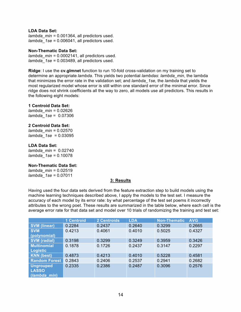
3: Results

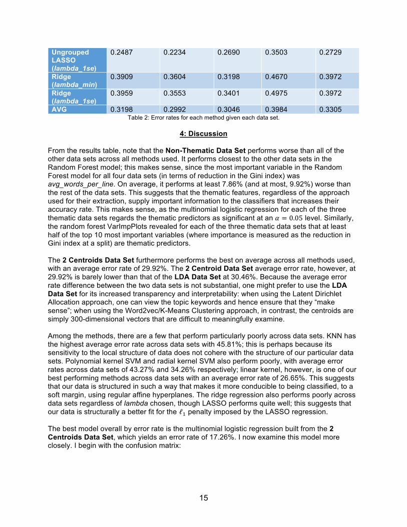
Having used the four data sets derived from the feature extraction step to build models using the machine learning techniques described above, I apply the models to the test set. I measure the accuracy of each model by its error rate: by what percentage of the test set poems it incorrectly attributes to the wrong poet. These results are summarized in the table below, where each cell is the average error rate for that data set and model over 10 trials of randomizing the training and test set: 1 Centroid 2 Centroids LDA Non-Thematic AVG

SVM (linear) 0.2284 0.2437 0.2640 0.3299 0.2665 SVM

(polynomial) 0.4213 0.4061 0.4010 0.5025 0.4327

SVM (radial) 0.3198 0.3299 0.3249 0.3959 0.3426 Multinomial

Logistic 0.1878 0.1726 0.2437 0.3147 0.2297

KNN (best) 0.4873 0.4213 0.4010 0.5228 0.4581 Random Forest 0.2843 0.2406 0.2537 0.2941 0.2682 Ungrouped

LASSO

(lambda_min)

0.2335 0.2386 0.2487 0.3096 0.2576

15

Ungrouped

LASSO

(lambda_1se)

0.2487 0.2234 0.2690 0.3503 0.2729

Ridge

(lambda_min) 0.3909 0.3604 0.3198 0.4670 0.3972

Ridge

(lambda_1se) 0.3959 0.3553 0.3401 0.4975 0.3972

AVG 0.3198 0.2992 0.3046 0.3984 0.3305 Table 2: Error rates for each method given each data set.

4: Discussion

From the results table, note that the Non-Thematic Data Set performs worse than all of the other data sets across all methods used. It performs closest to the other data sets in the Random Forest model; this makes sense, since the most important variable in the Random Forest model for all four data sets (in terms of reduction in the Gini index) was avg_words_per_line. On average, it performs at least 7.86% (and at most, 9.92%) worse than the rest of the data sets. This suggests that the thematic features, regardless of the approach used for their extraction, supply important information to the classifiers that increases their accuracy rate. This makes sense, as the multinomial logistic regression for each of the three thematic data sets regards the thematic predictors as significant at an 9 = 0.05 level. Similarly, the random forest VarImpPlots revealed for each of the three thematic data sets that at least half of the top 10 most important variables (where importance is measured as the reduction in Gini index at a split) are thematic predictors. The 2 Centroids Data Set furthermore performs the best on average across all methods used, with an average error rate of 29.92%. The 2 Centroid Data Set average error rate, however, at 29.92% is barely lower than that of the LDA Data Set at 30.46%. Because the average error rate difference between the two data sets is not substantial, one might prefer to use the LDA

Data Set for its increased transparency and interpretability: when using the Latent Dirichlet Allocation approach, one can view the topic keywords and hence ensure that they “make sense”; when using the Word2vec/K-Means Clustering approach, in contrast, the centroids are simply 300-dimensional vectors that are difficult to meaningfully examine. Among the methods, there are a few that perform particularly poorly across data sets. KNN has the highest average error rate across data sets with 45.81%; this is perhaps because its sensitivity to the local structure of data does not cohere with the structure of our particular data sets. Polynomial kernel SVM and radial kernel SVM also perform poorly, with average error rates across data sets of 43.27% and 34.26% respectively; linear kernel, however, is one of our best performing methods across data sets with an average error rate of 26.65%. This suggests that our data is structured in such a way that makes it more conducible to being classified, to a soft margin, using regular affine hyperplanes. The ridge regression also performs poorly across data sets regardless of lambda chosen, though LASSO performs quite well; this suggests that our data is structurally a better fit for the ℓ3 penalty imposed by the LASSO regression. The best model overall by error rate is the multinomial logistic regression built from the 2

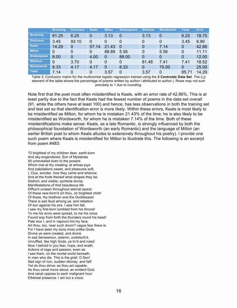
Centroids Data Set, which yields an error rate of 17.26%. I now examine this model more closely. I begin with the confusion matrix:

16

Browning Dickinson Keats Milton Shakespeare Whitman Wordsworth Yeats Error

Browning 81.25 6.25 0 3.13 0 3.13 0 6.25 18.75 Dickinson 3.45 93.10 0 0 0 0 0 3.45 6.90 Keats 14.29 0 57.14 21.43 0 0 7.14 0 42.86 Milton 0 0 0 88.89 5.56 0 5.56 0 11.11 Shakespeare 8.00 0 4.00 0 88.00 0 0 0 12.00 Whitman 0 3.70 0 0 0 81.48 7.41 7.41 18.52 Wordsworth 8.33 4.17 4.17 0 8.33 0 75.00 0 25.00 Yeats 7.14 0 0 3.57 0 3.57 0 85.71 14.29 Table 3: Confusion matrix for the multinomial logistic regression trained using the 2 Centroids Data Set. The (i,j) element of the table shows the percentage of poems written by author i attributed to author j. Rows may not sum

precisely to 1 due to rounding.

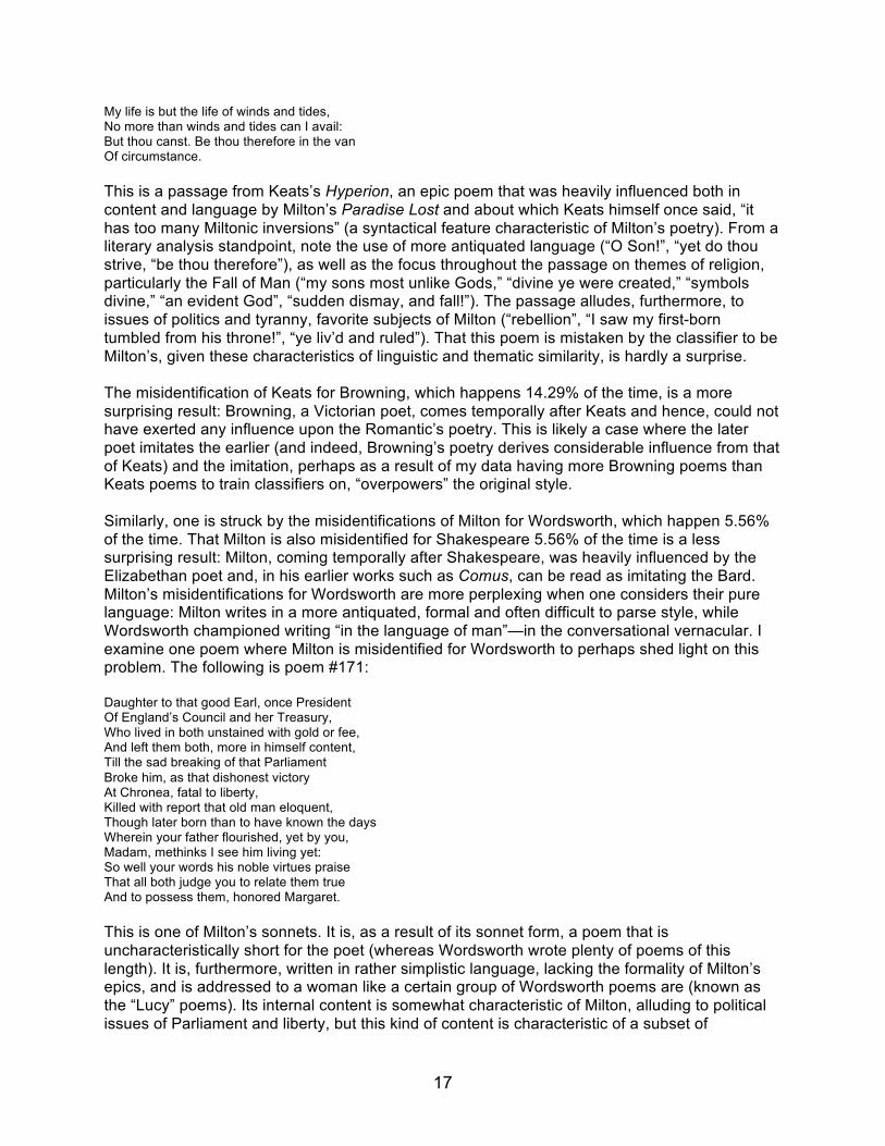
Note first that the poet most often misidentified is Keats, with an error rate of 42.86%. This is at least partly due to the fact that Keats had the fewest number of poems in the data set overall (91, while the others have at least 100) and hence, has less observations in both the training set and test set so that identification error is more likely. Within these errors, Keats is most likely to be misidentified as Milton, for whom he is mistaken 21.43% of the time; he is also likely to be misidentified as Wordsworth, for whom he is mistaken 7.14% of the time. Both of these misidentifications make sense: Keats, as a late Romantic, is strongly influenced by both the philosophical foundation of Wordsworth (an early Romantic) and the language of Milton (an earlier British poet to whom Keats alludes to extensively throughout his poetry). I provide one such poem where Keats is misidentified for Milton to illustrate this. The following is an excerpt from poem #483: "O brightest of my children dear, earth-born And sky-engendered, Son of Mysteries All unrevealed even to the powers Which met at thy creating; at whose joys And palpitations sweet, and pleasures soft, I, Clus, wonder, how they came and whence; And at the fruits thereof what shapes they be, Distinct, and visible; symbols divine, Manifestations of that beauteous life Diffus'd unseen throughout eternal space: Of these new-form'd art thou, oh brightest child! Of these, thy brethren and the Goddesses! There is sad feud among ye, and rebellion Of son against his sire. I saw him fall, I saw my first-born tumbled from his throne! To me his arms were spread, to me his voice Found way from forth the thunders round his head! Pale wox I, and in vapours hid my face. Art thou, too, near such doom? vague fear there is: For I have seen my sons most unlike Gods. Divine ye were created, and divine In sad demeanour, solemn, undisturb'd, Unruffled, like high Gods, ye liv'd and ruled: Now I behold in you fear, hope, and wrath; Actions of rage and passion; even as I see them, on the mortal world beneath, In men who die. This is the grief, O Son! Sad sign of ruin, sudden dismay, and fall! Yet do thou strive; as thou art capable, As thou canst move about, an evident God; And canst oppose to each malignant hour Ethereal presence: I am but a voice;

17

My life is but the life of winds and tides, No more than winds and tides can I avail: But thou canst. Be thou therefore in the van Of circumstance.

This is a passage from Keats’s Hyperion, an epic poem that was heavily influenced both in content and language by Milton’s Paradise Lost and about which Keats himself once said, “it has too many Miltonic inversions” (a syntactical feature characteristic of Milton’s poetry). From a literary analysis standpoint, note the use of more antiquated language (“O Son!”, “yet do thou strive, “be thou therefore”), as well as the focus throughout the passage on themes of religion, particularly the Fall of Man (“my sons most unlike Gods,” “divine ye were created,” “symbols divine,” “an evident God”, “sudden dismay, and fall!”). The passage alludes, furthermore, to issues of politics and tyranny, favorite subjects of Milton (“rebellion”, “I saw my first-born tumbled from his throne!”, “ye liv’d and ruled”). That this poem is mistaken by the classifier to be Milton’s, given these characteristics of linguistic and thematic similarity, is hardly a surprise. The misidentification of Keats for Browning, which happens 14.29% of the time, is a more surprising result: Browning, a Victorian poet, comes temporally after Keats and hence, could not have exerted any influence upon the Romantic’s poetry. This is likely a case where the later poet imitates the earlier (and indeed, Browning’s poetry derives considerable influence from that of Keats) and the imitation, perhaps as a result of my data having more Browning poems than Keats poems to train classifiers on, “overpowers” the original style. Similarly, one is struck by the misidentifications of Milton for Wordsworth, which happen 5.56% of the time. That Milton is also misidentified for Shakespeare 5.56% of the time is a less surprising result: Milton, coming temporally after Shakespeare, was heavily influenced by the Elizabethan poet and, in his earlier works such as Comus, can be read as imitating the Bard. Milton’s misidentifications for Wordsworth are more perplexing when one considers their pure language: Milton writes in a more antiquated, formal and often difficult to parse style, while Wordsworth championed writing “in the language of man”—in the conversational vernacular. I examine one poem where Milton is misidentified for Wordsworth to perhaps shed light on this problem. The following is poem #171: Daughter to that good Earl, once President Of England’s Council and her Treasury, Who lived in both unstained with gold or fee, And left them both, more in himself content, Till the sad breaking of that Parliament Broke him, as that dishonest victory At Chronea, fatal to liberty, Killed with report that old man eloquent, Though later born than to have known the days Wherein your father flourished, yet by you, Madam, methinks I see him living yet: So well your words his noble virtues praise That all both judge you to relate them true And to possess them, honored Margaret.

This is one of Milton’s sonnets. It is, as a result of its sonnet form, a poem that is uncharacteristically short for the poet (whereas Wordsworth wrote plenty of poems of this length). It is, furthermore, written in rather simplistic language, lacking the formality of Milton’s epics, and is addressed to a woman like a certain group of Wordsworth poems are (known as the “Lucy” poems). Its internal content is somewhat characteristic of Milton, alluding to political issues of Parliament and liberty, but this kind of content is characteristic of a subset of

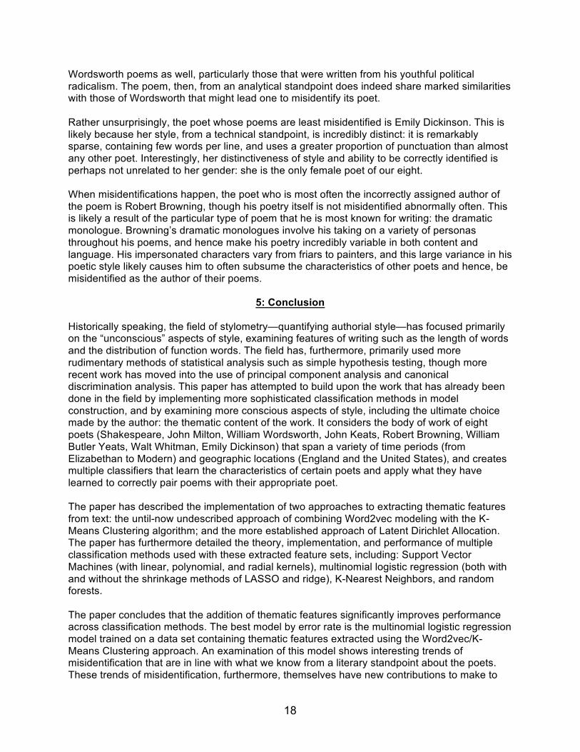
18

Wordsworth poems as well, particularly those that were written from his youthful political radicalism. The poem, then, from an analytical standpoint does indeed share marked similarities with those of Wordsworth that might lead one to misidentify its poet. Rather unsurprisingly, the poet whose poems are least misidentified is Emily Dickinson. This is likely because her style, from a technical standpoint, is incredibly distinct: it is remarkably sparse, containing few words per line, and uses a greater proportion of punctuation than almost any other poet. Interestingly, her distinctiveness of style and ability to be correctly identified is perhaps not unrelated to her gender: she is the only female poet of our eight. When misidentifications happen, the poet who is most often the incorrectly assigned author of the poem is Robert Browning, though his poetry itself is not misidentified abnormally often. This is likely a result of the particular type of poem that he is most known for writing: the dramatic monologue. Browning’s dramatic monologues involve his taking on a variety of personas throughout his poems, and hence make his poetry incredibly variable in both content and language. His impersonated characters vary from friars to painters, and this large variance in his poetic style likely causes him to often subsume the characteristics of other poets and hence, be misidentified as the author of their poems.

5: Conclusion

Historically speaking, the field of stylometry—quantifying authorial style—has focused primarily on the “unconscious” aspects of style, examining features of writing such as the length of words and the distribution of function words. The field has, furthermore, primarily used more rudimentary methods of statistical analysis such as simple hypothesis testing, though more recent work has moved into the use of principal component analysis and canonical discrimination analysis. This paper has attempted to build upon the work that has already been done in the field by implementing more sophisticated classification methods in model construction, and by examining more conscious aspects of style, including the ultimate choice made by the author: the thematic content of the work. It considers the body of work of eight poets (Shakespeare, John Milton, William Wordsworth, John Keats, Robert Browning, William Butler Yeats, Walt Whitman, Emily Dickinson) that span a variety of time periods (from Elizabethan to Modern) and geographic locations (England and the United States), and creates multiple classifiers that learn the characteristics of certain poets and apply what they have learned to correctly pair poems with their appropriate poet. The paper has described the implementation of two approaches to extracting thematic features from text: the until-now undescribed approach of combining Word2vec modeling with the K-Means Clustering algorithm; and the more established approach of Latent Dirichlet Allocation. The paper has furthermore detailed the theory, implementation, and performance of multiple classification methods used with these extracted feature sets, including: Support Vector Machines (with linear, polynomial, and radial kernels), multinomial logistic regression (both with and without the shrinkage methods of LASSO and ridge), K-Nearest Neighbors, and random forests. The paper concludes that the addition of thematic features significantly improves performance across classification methods. The best model by error rate is the multinomial logistic regression model trained on a data set containing thematic features extracted using the Word2vec/K-Means Clustering approach. An examination of this model shows interesting trends of misidentification that are in line with what we know from a literary standpoint about the poets. These trends of misidentification, furthermore, themselves have new contributions to make to

19

the literary understanding of each poet’s style. The fields of stylometry and literary analysis have much to learn from each other, and this paper hopes to have illustrated a small piece of this potential.

20

References

Antosch, F. "The Diagnosis of Literary Style with the Verb-Adjective Ratio." In Statistics and Style, Eds. L. Dolezet and R.W. Bailey. New York: American Elsevier, 1969.

Bailey, R.W. "Authorship Attribution in a Forensic Setting." Advances in Computer-aided Literary and Linguistic Research. Eds. D.E. Ager, F.E. Knowles and J. Smith. Birmingham: AMLC, 1979.

Binongo, J.N.G. “Who wrote the 15th book of Oz? An application of multivariate analysis to authorship attribution.” Chance, 16 (2003), 9-17.

Blei, D. M., A. Ng, and M. Jordan. “Latent Dirichlet Allocation.” Journal of Machine Learning Research, 3 (2003), 993-1022.

Brainerd, B. "On the Distinction Between a Novel and a Romance: A Discriminant Analysis.” Computers and Humanities, 7 (1973), 259-270.

Brinegar, C.S. "Mark Twain and the Quintus Curtius Snodgrass Letters: A Statistical Test of Authorship." Journal of the American Statistical Association, 58 (1963), 85-96.

Dabagh, R.H. “Authorship Attribution and Statistical Text Analysis.” Metodološki zveski, 4, 2 (2007), 149-163.

Fucks, W. "On the Mathematical Analysis of Style." Biometrika, 39 (1952), 122-129.

Fucks, W. and J. Lauter. "Mathematische Analyse des Literarischen Stils." In Mathematik und Dichtung. Eds. H. Kreuzer and R. Gunzenhausers. Munich: Nymphenburger Verlagsbucldaandlung, 1965.

Holmes, D.I. "A Stylometric Analysis of Mormon Scripture and Related Texts." Journal of the Royal Statistical Society (A), 155, 1 (1992), 91-120.

Mendenhall, T.C. "The Characteristic Curves of Composition." Science, IX (1887), 237-249.

Mikolov, M., K. Chen, G. Corrado, and J. Dean. “Efficient Estimation of Word Representations in Vector Space.” 2013.

Morton, A.Q. "The Authorship of Greek Prose." Journal of the Royal Statistical Society (A), 128 (1965), 169-233.

Mosteller, F. and D. L. Wallace. "Inference in an Authorship Problem." Journal of the American Statistical Association 58, no. 302 (1963): 275-309.

Mosteller, F. and D. L. Wallace. "Inference and Disputed Authorship: The Federalist." Reading, MA: Addison- Wesley, 1964.

Peng, R.D. and Hengartner, N.W. “Quantitative analysis of literary styles.” The American Statistician, 56 (2002), 175-185.

21

Williams, C.B. "A Note on the Statistical Analysis of Sentence-Length as a Criterion of Literary Style." Biometrika, 31 (1940), 356-361.

Yule, G.U. "On Sentence-Length as a Statistical Characteristic of Style in Prose, with Application to Two Cases of Disputed Authorship." Biometrika, 30 (1938), 363-390.

22

Appendix A: Titles and URLs of Project Gutenberg Texts Used

Shakespeare’s Sonnets http://www.gutenberg.org/files/1041/1041-h/1041-h.htm Milton: Minor Poems http://www.gutenberg.org/files/31706/31706-h/31706-h.htm The Poetical Words of John Milton http://www.gutenberg.org/files/1745/1745-h/1745-h.htm L’Allegro, Il Penseroso, Comus, and Lycidas http://www.gutenberg.org/cache/epub/397/pg397-images.html Paradise Lost http://www.gutenberg.org/files/20/20-h/20-h.htm Paradise Regained http://www.gutenberg.org/cache/epub/58/pg58-images.html The Poetical Works of William Wordsworth – Volume 1 http://www.gutenberg.org/files/10219/10219-h/10219-h.htm The Poetical Works of William Wordsworth – Volume 2 http://www.gutenberg.org/files/12145/12145-h/12145-h.htm The Poetical Works of William Wordsworth – Volume 3 http://www.gutenberg.org/files/12383/12383-h/12383-h.htm The Poetical Works of William Wordsworth – Volume 4 http://www.gutenberg.org/files/32459/32459-h/32459-h.htm The Poetical Works of William Wordsworth – Volume 5 http://www.gutenberg.org/files/56361/56361-h/56361-h.htm The Poetical Works of William Wordsworth – Volume 6 http://www.gutenberg.org/files/47651/47651-h/47651-h.htm The Poetical Works of William Wordsworth – Volume 7 http://www.gutenberg.org/files/47143/47143-h/47143-h.htm The Poetical Works of William Wordsworth – Volume 8 http://www.gutenberg.org/files/52836/52836-h/52836-h.htm Keats: Poems Published in 1820 http://www.gutenberg.org/files/23684/23684-h/23684-h.htm Poems, 1817 http://www.gutenberg.org/files/8209/8209-h/8209-h.htm Endymion: A Poetic Romance http://www.gutenberg.org/files/24280/24280-h/24280-h.htm The Complete Poetic and Dramatic Works of Robert Browning http://www.gutenberg.org/files/50954/50954-h/50954-h.htm The Collected Works in Verse and Prose of William Butler Yeats – Volume 1 http://www.gutenberg.org/files/49608/49608-h/49608-h.htm The Collected Works in Verse and Prose of William Butler Yeats – Volume 2 http://www.gutenberg.org/files/49609/49609-h/49609-h.htm The Collected Works in Verse and Prose of William Butler Yeats – Volume 3 http://www.gutenberg.org/files/49610/49610-h/49610-h.htm The Collected Works in Verse and Prose of William Butler Yeats – Volume 4 http://www.gutenberg.org/files/49611/49611-h/49611-h.htm The Collected Works in Verse and Prose of William Butler Yeats – Volume 5 http://www.gutenberg.org/files/49612/49612-h/49612-h.htm The Collected Works in Verse and Prose of William Butler Yeats – Volume 6 http://www.gutenberg.org/files/49613/49613-h/49613-h.htm The Collected Works in Verse and Prose of William Butler Yeats – Volume 7 http://www.gutenberg.org/files/49614/49614-h/49614-h.htm The Collected Works in Verse and Prose of William Butler Yeats – Volume 8 http://www.gutenberg.org/files/49615/49615-h/49615-h.htm Leaves of Grass http://www.gutenberg.org/files/1322/1322-h/1322-h.htm Poems by Emily Dickinson, Three Series, Complete http://www.gutenberg.org/files/12242/12242-h/12242-h.htm