Quantifying the Amount and Economic Impacts of …sustainableferc.org/wp-content/uploads/2014/09/Brattle...Quantifying the Amount and Economic Impacts of Missing Energy Efficiency

Quantifying the Amount and Economic Impacts of Missing Energy Efficiency in PJM’s Load Forecast

PREPARED FOR

The Sustainable FERC Project

PREPARED BY

Ahmad Faruqui, Ph.D.

Sanem Sergici, Ph.D.

Kathleen Spees, Ph.D.

September 2014

This report was prepared for The Sustainable FERC Project, a coalition of national and regional

clean energy advocates and other public interest organizations focused on breaking down federal

regulatory barriers to the grid integration of renewable energy demand-side resources. All results

and any errors are the responsibility of the authors alone and do not represent the opinion of The

Brattle Group, Inc. or its clients.

We acknowledge the valuable contributions of Allison Clements and John Moore of The

Sustainable FERC Project to this report. We would like to thank Ioanna Karkatsouli of The

Brattle Group for excellent research assistance.

Copyright © 2014 The Brattle Group, Inc.

i | brattle.com

Table of Contents

I. Introduction ................................................................................................................................. 1

II. Projecting EE Missing from the Load Forecast .......................................................................... 2

III. Market Modeling Approach ........................................................................................................ 4

A. Capacity Price Impacts ....................................................................................................... 5

B. Energy Price Impacts ......................................................................................................... 6

IV. Results .......................................................................................................................................... 7

V. Study Caveats ............................................................................................................................... 8

APPENDIX A—PowerPoint Presentation of the Study Assumptions, Methodology and Approach

1 | brattle.com

I. Introduction

In ISO New England (ISO-NE) and the New York ISO (NYISO), targeted efforts have been

undertaken to capture the effects of existing and planned energy efficiency programs that may be

unaccounted for in the forecasting process. Such targeted efforts do not exist for the PJM

Interconnection (PJM). This project was undertaken to examine whether there is any “missing

energy efficiency” in PJM since it might represent an opportunity for reducing environmental

impacts and customer costs.

PJM’s load forecast currently accounts for energy efficiency (EE) in two ways: (1) historical

efficiency embedded in econometric forecasts, and (2) supply-side EE that clears in the

Reliability Pricing Model (RPM). However, this approach does not capture the existing EE that

did not bid into/clear in the RPM, or any new/incremental EE programs predicted beyond the

three year forward capacity market window. As noted above, both ISO-NE and NYISO have

addressed these issues in their load forecasting processes to account for the full effects of the EE

investments and produce a more accurate load forecast.

In this study, we undertake an analysis to: (1) determine whether a significant amount of EE is

unaccounted for in PJM’s regional forecasts; (2) determine the impact of the unaccounted EE on

load growth; and (3) quantify the level of customer cost impacts that would result from

incorporating the unaccounted EE in the forecast, by affecting energy and capacity prices and

avoiding some capacity procurements. In this study, we do not quantify the potential benefits of

avoided transmission and distribution investments that would emerge from a more complete

treatment of the EE impacts in the load forecasting process.

Our study is an effort to gauge the magnitude of the EE missing from the load forecasts based on

publicly available data and reasonable assumptions. It is important to note that our study is not

intended to substitute for a coordinated effort that might be led by PJM to project EE savings in

the forecast period and account for them in their load forecasting effort. It is also not intended as

a comprehensive review or commentary on PJM’s overall load forecasting method (since energy

efficiency is only a small component thereof), or be a substitute for a more rigorous and in-depth

analysis that would account for the effect that all existing and planned energy efficiency savings

may have on PJM market and transmission planning outcomes. Such a comprehensive effort

2 | brattle.com

would require significant stakeholder involvement and PJM effort, which may be undertaken in

the future.

This executive summary report is organized as follows. Section II describes the methodology used

for projecting the EE missing from PJM’s load forecasting framework. Section III provides a brief

overview of the approach used for modeling the capacity and energy cost impacts after properly

accounting for the missing EE. Section IV summarizes the findings of our study. We have also

included an Appendix to this report, a PowerPoint presentation, which provides the details of

our assumption, methodology, and findings.

II. Projecting EE Missing from the Load Forecast

The biggest implications of PJM’s forecast are in the capacity market and in long-term

transmission planning. Peak demand forecasts in each location are the primary determinant of

quantity procured in the capacity market. Some new EE offers into the capacity market as

supply-side resources and so are already counted, but if any “missing EE” does not participate,

overall capacity requirements will be overstated and over procurement of capacity will occur.

For long-term planning, PJM’s energy load forecast assumes that the historical data already

embeds the historical EE impacts. It assumes that future forecasts reflect similar trends in EE and

thus no EE adjustments are made for any missing EE. PJM’s peak demand forecasts account for

the impact of approved EE programs that cleared in the RPM. The amount cleared in the last

auction is held constant for the remainder of the forecast. However, there still might be some

“missing EE” that does not offer into RPM or that is projected for years beyond the RPM

timeframe.

This treatment of EE in PJM’s load forecasting process is likely to understate the full benefits of

EE investments. As indicated earlier, both ISO-NE and NYISO incorporate into their forecasts

the amount of EE that is forecasted beyond the three-year forward capacity planning period and

is incremental to the EE that cleared in the capacity auctions.

We had originally planned to follow an approach similar to the one used by the NYISO and ISO-

NE to project the EE savings by zone. However, this approach required information that would

only be obtained through a coordinated stakeholder process as employed by the ISO-NE and

NYISO. Therefore, we adopted an alternative approach that is based on compiling EE

projections using publicly available filings for each of the 20 utility zones in PJM. We relied on

3 | brattle.com

three major data sources to compile the EE projections for each of the zones: (1) utility/state

integrated resource plans (IRP); (2) utility/state demand side management (DSM) filings; and

(3) EIA Form 861.

We used one of two approaches to generate “incremental EE projections” for the 2014–2022 time

period, for all but two very small zones in the PJM footprint1: (1) for some zones that included

utility EE projections for 2014–2016, we used the most recent forecast value for each of the

remaining years in the forecast period (four zones included projections for longer time periods);

and (ii) for the several zones that did not have the EE projections, we used the 2012 actual EE

savings reported in the EIA 861 data for each year of the forecast period.

We also made an effort to avoid double-counting of EE that is already included in PJM’s load

forecasts. PJM load forecasts reflect some amount of EE following a trend similar to the

historical trend. To account for this embedded EE and avoid double-counting, we:

Take the average EE achieved in each zone between 2000–2012, and assume that

this captures the historical trend and reflects the embedded EE;

Subtract this embedded EE amount from each year of the projected “incremental

EE” series starting with 2014;

Calculate “cumulative EE” projections starting with 2014 after obtaining the

incremental EE net off historical trend EE;

Calculate the “peak value (MW)” of the cumulative EE projections (GWh) by

using zone specific historical MW/GWh ratios.

As a result of this effort, we project that the cumulative GWh savings from new EE (relative to

2013) will reach 11,213 GWh (1.3% of load) in 2017 and 27,245 GWh (3% of load) in 2022.

PJM’s current energy forecasting framework does not account for this additive EE that is

projected to come online during the forecast period in excess of the new EE that is already

embedded in PJM’s energy forecasts.

Similarly, the cumulative MW savings from new EE (relative to 2013) will reach 1,817 MW

(1.1% of peak demand) in 2017 and 4,391 MW (2.5% of load) in 2022. PJM’s current peak

demand framework only accounts for the impact of approved EE programs that cleared in the

1 We were not able to find reliable data for these two very small zones.

4 | brattle.com

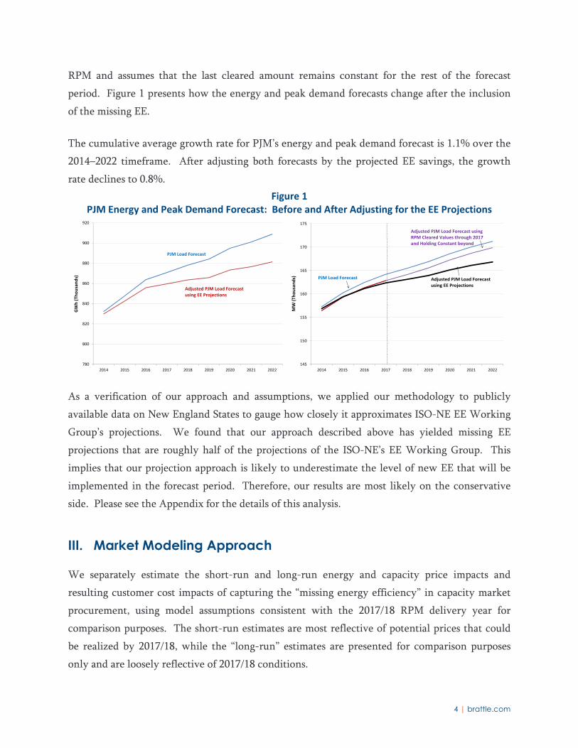
RPM and assumes that the last cleared amount remains constant for the rest of the forecast

period. Figure 1 presents how the energy and peak demand forecasts change after the inclusion

of the missing EE.

The cumulative average growth rate for PJM’s energy and peak demand forecast is 1.1% over the

2014–2022 timeframe. After adjusting both forecasts by the projected EE savings, the growth

rate declines to 0.8%.

Figure 1 PJM Energy and Peak Demand Forecast: Before and After Adjusting for the EE Projections

As a verification of our approach and assumptions, we applied our methodology to publicly

available data on New England States to gauge how closely it approximates ISO-NE EE Working

Group’s projections. We found that our approach described above has yielded missing EE

projections that are roughly half of the projections of the ISO-NE’s EE Working Group. This

implies that our projection approach is likely to underestimate the level of new EE that will be

implemented in the forecast period. Therefore, our results are most likely on the conservative

side. Please see the Appendix for the details of this analysis.

III. Market Modeling Approach

We separately estimate the short-run and long-run energy and capacity price impacts and

resulting customer cost impacts of capturing the “missing energy efficiency” in capacity market

procurement, using model assumptions consistent with the 2017/18 RPM delivery year for

comparison purposes. The short-run estimates are most reflective of potential prices that could

be realized by 2017/18, while the “long-run” estimates are presented for comparison purposes

only and are loosely reflective of 2017/18 conditions.

780

800

820

840

860

880

900

920

2014 2015 2016 2017 2018 2019 2020 2021 2022

GWh (Th

ousands)

PJM Load Forecast

Adjusted PJM Load Forecastusing EE Projections

145

150

155

160

165

170

175

2014 2015 2016 2017 2018 2019 2020 2021 2022

MW (Th

ousands) PJM Load Forecast

Adjusted PJM Load Forecast usingRPM Cleared Values through 2017 and Holding Constant beyond


5 | brattle.com

The total cost impact has two components: capacity and energy cost impacts. After accounting

for the missing EE in the forecasts, total capacity costs go down, which represents the largest of

the two impacts, whereas the total energy impacts go up, which represents the smaller of the two

impacts. The net impact is a reduction in the total customer costs, as we present in Section IV—

Results. It is important to note that this study focuses on the impacts of accounting for the

projected EE only, which changes the procured capacity using a more accurate load forecast,

leaving the realized load unchanged. This is different from implementing new EE, which would

reduce both procured capacity and energy, resulting in cost savings in both markets. We provide

the details of this distinction in the Appendix.

Below, we provide a brief overview of the modeling approach. For details, please see the

Appendix.

A. Capacity Price Impacts

In the short-run, we replicate the 2017/18 Base Residual Auction (BRA) clearing results as our

business as usual (BAU) scenario. We reflect PJM’s administrative demand curve and

transmission parameters for 2017/18 using a simulation tool that replicates PJM’s locational

auction clearing mechanics.2 Supply in each location reflects a generic supply curve shape, as

calibrated to match each location’s offered quantity, cleared price, and cleared quantity. In our

scenario cases, we adjust PJM’s load forecast and demand curve quantity points downward

appropriately in each location consistent with the projected level of energy efficiency. These

downward adjustments to demand result in substantial reductions in customer costs because:

(a) capacity prices drop substantially due to the relatively steep supply curve, and (b) the quantity

of capacity procured at those prices also drops.

In the long-run, customer capacity cost impacts will decline because prices must converge to the

long-run marginal cost of building generation supply, or the Net Cost of New Entry (Net CONE).

In our BAU scenario, we assume that: (i) prices in all regions will converge to the administrative

Net CONE estimate of the Mid-Atlantic Area Council (MAAC) Locational Deliverability Area

(LDA), and that (ii) quantities will converge to the demand curve quantity at point “b” where the

demand curve price equals Net CONE. In scenario cases, we adjust this procured quantity

2 The tool does not account for the effects of sub-annual resource constraints or maximum import

constraints.

6 | brattle.com

downward, consistent with the projected level of energy efficiency adjustment. Capacity prices

also drop somewhat in these scenario cases, accounting for the fact that the lower cleared

capacity reserve margin will correspond to higher energy prices, higher supplier energy margins,

and a lower Net CONE. Therefore in the long run, capacity costs will also drop based on a

decline in both capacity prices and quantities, but the capacity price impact is much smaller in

the long run than in the short run (while the quantity impact is of a similar size).

A true long-run capacity or energy price estimate would necessarily reflect a more distant

delivery year, and so the prices we present must be interpreted as having an illustrative

magnitude compared to 2017/18 without reflecting all other changes that may occur between

then and a true long-term equilibrium year. Acknowledging this nuance, we present this long-

run estimate to illustrate the fact that the relatively larger capacity price impacts that we

estimate using a short-run approach must be interpreted as temporary. Such reductions in

capacity prices cannot be sustained into perpetuity, because low prices would result in fewer

supply developments and more retirements until prices would ultimately rise back to sustainable

long-run levels. In the long term, net customer costs still decline with a downward adjustment

to load forecast, but the magnitude of the impact is much smaller.

B. Energy Price Impacts

We similarly calculate short-run and long-run energy price impacts consistent with year

2017/18. We estimate BAU energy prices in each location based on monthly forward curves at

PJM West Hub. We then apply locational adjustments based on long-term Financial

Transmission Rights (FTR) auction results, to develop monthly energy price estimates in each

PJM zone. We assume the same BAU energy prices in both the short-run and long-run cases.

Again, we make this long-run assumption for illustrative purposes, although we acknowledge

that a true long-run energy price estimate would have lower reserve margins and therefore

higher energy prices than in the short run, if all other factors remained constant.

We then estimate the energy price increase that would result from a reduction in PJM’s load

forecast. Energy prices would increase with a reduction in load forecast because: (1) the quantity

of capacity procured in the capacity market would decrease as above; (2) true peak load realized

in the delivery year will stay the same, because the PJM forecast has no impact on the actual

peak load that will ultimately be realized; and (3) the decline in realized supply relative to

realized demand corresponds to a lower reserve margin and higher energy prices.

7 | brattle.com

To estimate the magnitude of this energy price increase, we develop a relationship between

monthly realized energy prices and monthly realized reserve margins on a zonal basis, separately

for on-peak and off-peak hours3. Using this relationship, we estimate the percentage increase

that we would expect in on- and off-peak energy prices, corresponding to the same reduction in

procured capacity as estimated above. This increase in energy prices offsets the cost savings from

reductions in capacity prices and quantities.

Finally, we note that we believe that this energy price impact reflects a high-end estimate of the

potential energy price impacts from such a downward adjustment to load forecast (in both short-

and long-term scenarios). One could argue that the realized reserve margins would not change

even if forward procured capacity quantity does change. This is because PJM procures 97.5% of

its reliability requirement in the 3-year forward BRA, and procures the remaining 2.5% in the

shorter-term Incremental Auctions (IAs). It is plausible that shorter-term forecasts would

recognize a reduced load associated with EE, thereby avoiding some of that quantity

procurement. We do not account for these or other potential short-term effects from the IAs in

our analysis.

IV. Results

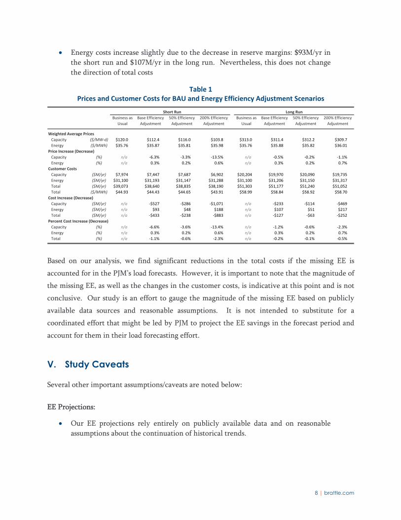
Table 1 summarizes the resulting capacity prices, energy prices, and customer costs under short-

run and long-run situations. We report results under our BAU case, and after adjusting the load

forecast downward by 50%, 100% (Base Efficiency Adjustment), and 200% of our projected

energy efficiency. As explained above, realized customer costs go down in both cases, with the

largest impacts being reductions in capacity procurement costs in the short run. More

specifically:

Total customer costs drop by $433M/yr in the short run and by $127M/yr in the

long run.

The largest cost reduction comes from reduction in capacity procurement costs:

$527M/yr in the short run and $233M/yr in the long run.

3 BAU energy prices reflect forward curves as of January 2014, while more recent forward curves would

reflect higher energy prices.

8 | brattle.com

Energy costs increase slightly due to the decrease in reserve margins: $93M/yr in

the short run and $107M/yr in the long run. Nevertheless, this does not change

the direction of total costs

Table 1 Prices and Customer Costs for BAU and Energy Efficiency Adjustment Scenarios

Based on our analysis, we find significant reductions in the total costs if the missing EE is

accounted for in the PJM’s load forecasts. However, it is important to note that the magnitude of

the missing EE, as well as the changes in the customer costs, is indicative at this point and is not

conclusive. Our study is an effort to gauge the magnitude of the missing EE based on publicly

available data sources and reasonable assumptions. It is not intended to substitute for a

coordinated effort that might be led by PJM to project the EE savings in the forecast period and

account for them in their load forecasting effort.

V. Study Caveats

Several other important assumptions/caveats are noted below:

EE Projections:

Our EE projections rely entirely on publicly available data and on reasonable

assumptions about the continuation of historical trends.

Short Run Long Run

Business as

Usual

Base Efficiency

Adjustment

50% Efficiency

Adjustment

200% Efficiency

Adjustment

Business as

Usual

Base Efficiency

Adjustment

50% Efficiency

Adjustment

200% Efficiency

Adjustment

Weighted Average Prices

Capacity ($/MW‐d) $120.0 $112.4 $116.0 $103.8 $313.0 $311.4 $312.2 $309.7

Energy ($/MWh) $35.76 $35.87 $35.81 $35.98 $35.76 $35.88 $35.82 $36.01

Price Increase (Decrease)

Capacity (%) n/a ‐6.3% ‐3.3% ‐13.5% n/a ‐0.5% ‐0.2% ‐1.1%

Energy (%) n/a 0.3% 0.2% 0.6% n/a 0.3% 0.2% 0.7%

Customer Costs

Capacity ($M/yr) $7,974 $7,447 $7,687 $6,902 $20,204 $19,970 $20,090 $19,735

Energy ($M/yr) $31,100 $31,193 $31,147 $31,288 $31,100 $31,206 $31,150 $31,317

Total ($M/yr) $39,073 $38,640 $38,835 $38,190 $51,303 $51,177 $51,240 $51,052

Total ($/MWh) $44.93 $44.43 $44.65 $43.91 $58.99 $58.84 $58.92 $58.70

Cost Increase (Decrease)

Capacity ($M/yr) n/a ‐$527 ‐$286 ‐$1,071 n/a ‐$233 ‐$114 ‐$469

Energy ($M/yr) n/a $93 $48 $188 n/a $107 $51 $217

Total ($M/yr) n/a ‐$433 ‐$238 ‐$883 n/a ‐$127 ‐$63 ‐$252

Percent Cost Increase (Decrease)

Capacity (%) n/a ‐6.6% ‐3.6% ‐13.4% n/a ‐1.2% ‐0.6% ‐2.3%

Energy (%) n/a 0.3% 0.2% 0.6% n/a 0.3% 0.2% 0.7%

Total (%) n/a ‐1.1% ‐0.6% ‐2.3% n/a ‐0.2% ‐0.1% ‐0.5%

9 | brattle.com

Capacity Related:

Our capacity model assumes short-term supply offers would be totally unaffected

by changes to administrative demand.

Short- and long-term effects do not account for the effects of the 2.5% holdback

(capacity procured at the incremental auctions), sub-annual resource constraints,

or maximum import constraints.

Long-term effects assume all locations converge to the same Net CONE, and

reflect a rough, approximate relationship between energy prices and energy

margins.

Energy Related:

BAU energy prices reflect forward curves current as of January 2014; forward

curves have increased since that time, which implies that the total customer cost

reduction estimated in our analysis would be slightly lower.

“Long-term” case for both energy and capacity is illustrative in magnitude relative

to the 2017/18 delivery year, but does not consider other factors that would

change between then and a true long-term equilibrium, including other changes

to supply, demand, and fuel prices among others.

Other:

This study does not constitute a comprehensive review of PJM’s load forecast, but

only focuses on a small component dealing with the effects of energy efficiency.

This study does not account for the potential benefits of avoided transmission and

distribution investments that might emerge from a more complete treatment of

the EE impacts in the load forecasting process.

This study was completed before the issuance of proposed regulations pursuant to

Section 111(d) of the Clean Air Act and therefore relied on the historical trends

for projecting future EE. With the renewed emphasis on EE with Section 111(d),

the future EE trends might be significantly different from that observed during

the historical period and may yield larger amounts of EE than is projected in this

analysis.

| brattle.com

APPENDIX A

PowerPoint Presentation of the

Study Assumptions, Methodology and Approach

Copyright © 2014 The Brattle Group, Inc.

Measuring the Presence and Effect of Energy Efficiency in the PJM’s Planning and Market Functions

Sustainable FERC

Ahmad Faruqui, Ph.D.Sanem Sergici, Ph.D.Kathleen Spees, Ph.D.

September 2014

Prepared by

Prepared fo r

Preliminary Draft Not for Citation or Distribution| brattle.com1

Outline  Background

 Objectives of the Study

  Projecting EE “Missing” from the Load Forecast

 Modeling Energy and Capacity Price Impacts after Accounting for the Missing EE

  Results

  Study Caveats

  Appendices


Study Rationale — A Statement from NRDC  The Sustainable FERC Project and clean energy advocates in PJM havewitnessed the impact of targeted efforts to capture existing andplanned energy efficiency in resource adequacy and long‐termplanning load forecasts in ISO‐NE and NYISO. We commissioned astudy to examine whether any “missing energy efficiency” also existsin the PJM load forecasting process that might involve opportunity forreduced environmental impacts and customer cost savings.

  The Brattle analysis described herein contributes to that examination.It is not intended as a comprehensive review or commentary on PJM’soverall load forecasting method (only a small component thereof), oras a substitute for a more rigorous and in‐depth analysis of thepotential impact that accounting for all existing and planned energyefficiency savings may have on PJM market and transmission planningoutcomes. Such a comprehensive effort would require significantstakeholder involvement and PJM effort.


Background

  PJM’s load forecast current accounts for energy efficiency (EE) intwo ways: (1) historical efficiency embedded in econometricforecasts, and (2) supply‐side EE that clears in the ReliabilityPricing Model (RPM)

  However, this approach does not capture:

▀ existing EE that did not bid into or clear in the RPM

▀ new/incremental EE programs predicted beyond the three yearforward capacity market window

  Both ISO‐NE and NYISO have addressed this issue in their loadforecasting process, in order to account for the full effects ofthe EE investments and produce a more accurate load forecast


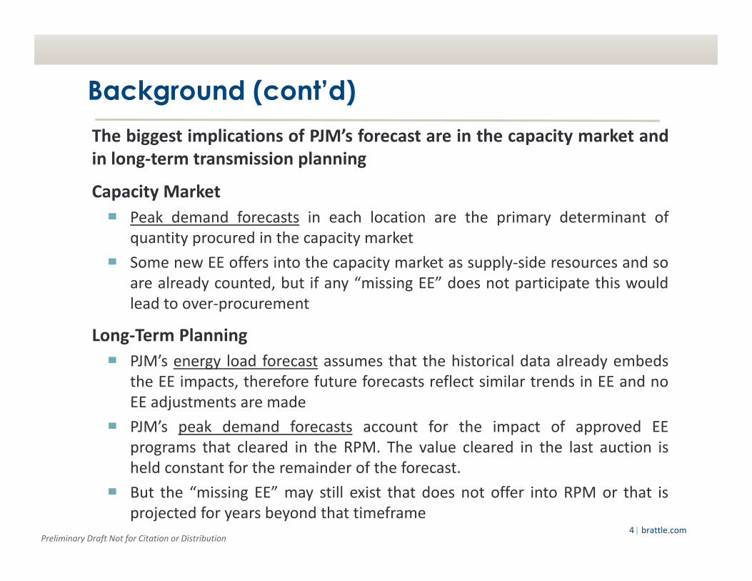
Background (cont’d)The biggest implications of PJM’s forecast are in the capacity market andin long‐term transmission planning

Capacity Market

▀ Peak demand forecasts in each location are the primary determinant ofquantity procured in the capacity market

▀ Some new EE offers into the capacity market as supply‐side resources and soare already counted, but if any “missing EE” does not participate this wouldlead to over‐procurement

Long‐Term Planning

▀ PJM’s energy load forecast assumes that the historical data already embedsthe EE impacts, therefore future forecasts reflect similar trends in EE and noEE adjustments are made

▀ PJM’s peak demand forecasts account for the impact of approved EEprograms that cleared in the RPM. The value cleared in the last auction isheld constant for the remainder of the forecast.

▀ But the “missing EE” may still exist that does not offer into RPM or that isprojected for years beyond that timeframe


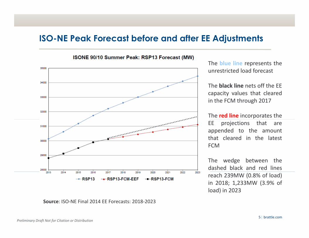
ISO-NE Peak Forecast before and after EE Adjustments

  Source: ISO‐NE Final 2014 EE Forecasts: 2018‐2023

The blue line represents theunrestricted load forecast

The black line nets off the EEcapacity values that clearedin the FCM through 2017

The red line incorporates theEE projections that areappended to the amountthat cleared in the latestFCM

The wedge between thedashed black and red linesreach 239MW (0.8% of load)in 2018; 1,233MW (3.9% ofload) in 2023


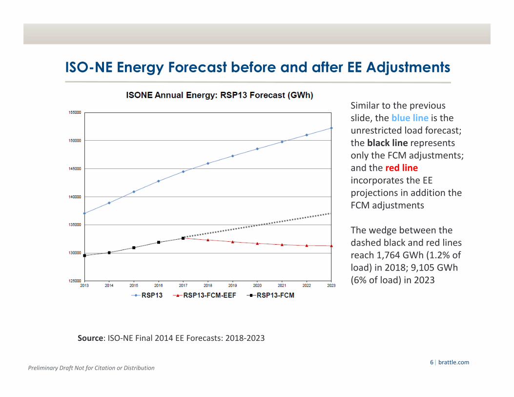
ISO-NE Energy Forecast before and after EE Adjustments

  Source: ISO‐NE Final 2014 EE Forecasts: 2018‐2023

Similar to the previous slide, the blue line is the unrestricted load forecast; the black line represents only the FCM adjustments; and the red line incorporates the EE projections in addition the FCM adjustments

The wedge between the dashed black and red lines reach 1,764 GWh (1.2% of load) in 2018; 9,105 GWh(6% of load) in 2023


Objectives of the Study

 We have three main objectives with this study:

(1) Determine whether significant amount of EE is unaccounted forin PJM’s regional forecasts;

(2) Determine the impact of the unaccounted EE on load growth;

(3) Quantify the level of customer benefits that would result fromincorporating the unaccounted EE in the forecast, in the form ofavoided capacity and energy payments


Projecting EE “Missing” from the Load Forecast We originally planned to build a budget/cost based model (similarto those used by the NYISO and ISO‐NE) to project the EE savingsby zone

▀ This model takes the projected DSM budget for a given utility anddivide it by the production cost rate, i.e., cost of achieving 1 MWh ofenergy savings, to back out the projected savings

  It quickly became clear that these budget estimates are notreadily available and would not be possible to obtain without aStakeholder process, as employed by the ISO‐NE

  Therefore, we adopted an alternative approach which is based oncompiling EE projections using publicly available data for each ofthe PJM zones


Projecting Missing EE We relied on three major data sources to compile the EE projections foreach of the zones:

▀ Utility or State Integrated Resource Plans (IRP)

▀ Utility or State Demand Side Management (DSM) filings

▀ EIA Form 861

We used one of two approaches for each of the zones to project the EEsavings for the 2014 – 2022 time frame:

(1) Some zones included EE projections for 2014‐2016, we used the lastavailable forecast value for each of the remaining years in the forecast period(four zones included projections for longer time periods)

(2) Several zones did not have the EE projections, for those we used the 2012actual EE savings reported in the EIA 861 data for each year of the forecastperiod


Projecting Missing EE  Using the approach introduced in the previous slide, we generate“incremental EE projections” for all but two very small zones in thePJM footprint

  PJM’s load forecasts already include some “embedded” EE. Thisimplies that the load forecasts already reflect some amount of EEfollowing a trend similar to the historical trend. To account for this

embedded EE and avoid double counting, we:

▀ Take the average EE achieved in each zone between 2000‐2012, andassume that this captures the historical trend and reflects the embeddedEE

▀ Subtract this embedded EE amount from each year of the projected“incremental EE” series starting with 2014

▀ Calculate “cumulative EE” projections starting with 2014 after obtainingthe incremental EE net off historical trend EE

▀ Calculate the “peak value (MW)” of the cumulative EE projections (GWh)by using zone specific historical MW/GWh ratios


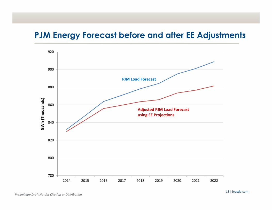
We find that significant amount of EE may be unaccounted for in PJM’s energy forecasts We project that the cumulative GWh savings from new EE(relative to 2013) will reach 11,213 GWh (1.3% of load) in 2017and 27,245 GWh (3% of load) in 2022

▀ PJM’s current energy forecasting framework does not account fornew EE that is projected to come online during the forecast periodin excess of the new EE that is already implied by the embeddedEE in the historical period

  The cumulative average growth rate for PJM’s energy forecast is1.1% over the 2014‐2022 timeframe. After adjusting the energyforecasts by the projected EE savings, the growth rate declinesto 0.8%


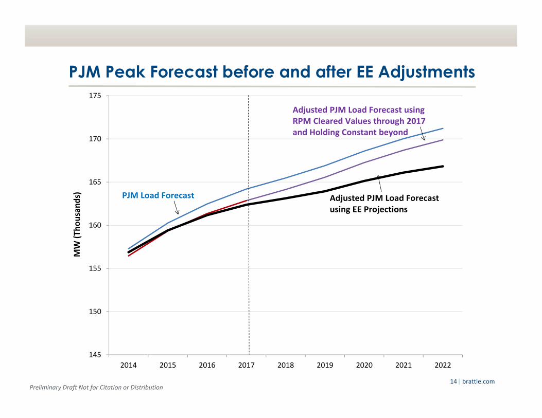
We find that significant amount of EE may be unaccounted for in PJM’s peak forecasts

 We project that the cumulative MW savings from new EE(relative to 2013) will reach 1,817 MW (1.1% of peak demand)in 2017 and 4,391 MW (2.5% of load) in 2022

▀ PJM’s current peak demand framework account for the impact ofapproved EE programs that cleared in the RPM. It does notaccount for the new EE beyond the RPM delivery years

  The cumulative average growth rate for PJM’s peak forecast is 1.1% over the 2014‐2022 timeframe. After adjusting the peak forecasts by the projected EE savings, the growth rate declines to 0.8%


PJM Energy Forecast before and after EE Adjustments

780

800

820

840

860

880

900

920

2014 2015 2016 2017 2018 2019 2020 2021 2022

GWh (Th

ousands)

PJM Load Forecast



PJM Peak Forecast before and after EE Adjustments

145

150

155

160

165

170

175

2014 2015 2016 2017 2018 2019 2020 2021 2022

MW (Th

ousands) PJM Load Forecast

Adjusted PJM Load Forecast usingRPM Cleared Values through 2017 and Holding Constant beyond



Modeling Energy and Capacity Price Impacts of Accounting for the Missing EE▀ We estimate both short‐run and long‐run impacts on capacity and energy prices, and associated customer costs if the PJM load forecast were adjusted downward to account for the “missing EE”

▀ Use 2017/18 delivery year as the basis for comparison

▀ Capacity: Costs go down (biggest effect)− Short‐run prices and costs are both down due to reduced demand

− Long‐run price will revert to the Net Cost of New Entry (CONE) with or without the EE adjustment (Net CONE also varies slightly with the change in energy price), but costs are still reduced because of the lower quantity of procurement

▀ Energy: Costs go up (smaller effect)− True load stays the same regardless of how PJM forecasts load and EE

− But prices would go up if PJM buys less supply through the capacity market, resulting in lower realized reserve margins

− Arguably, this effect could be small or zero if short‐term supply adjustments would correct for the over‐forecast before delivery even without this proposed adjustment to EE


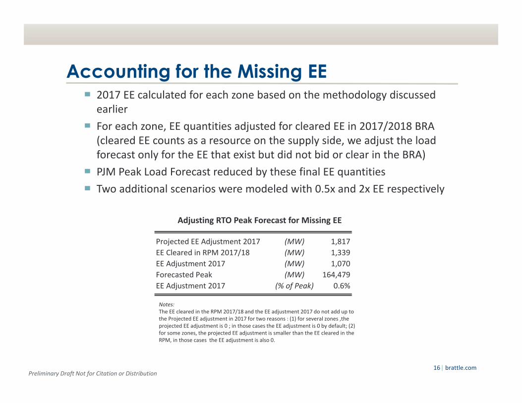
Accounting for the Missing EE▀ 2017 EE calculated for each zone based on the methodology discussed earlier

▀ For each zone, EE quantities adjusted for cleared EE in 2017/2018 BRA (cleared EE counts as a resource on the supply side, we adjust the load forecast only for the EE that exist but did not bid or clear in the BRA)

▀ PJM Peak Load Forecast reduced by these final EE quantities

▀ Two additional scenarios were modeled with 0.5x and 2x EE respectively

Adjusting RTO Peak Forecast for Missing EE

Notes:The EE cleared in the RPM 2017/18 and the EE adjustment 2017 do not add up to the Projected EE adjustment in 2017 for two reasons : (1) for several zones ,the projected EE adjustment is 0 ; in those cases the EE adjustment is 0 by default; (2) for some zones, the projected EE adjustment is smaller than the EE cleared in the RPM, in those cases the EE adjustment is also 0.

Projected EE Adjustment 2017 (MW) 1,817

EE Cleared in RPM 2017/18 (MW) 1,339

EE Adjustment 2017 (MW) 1,070

Forecasted Peak (MW) 164,479

EE Adjustment 2017 (% of Peak) 0.6%


$0

$100

$200

$300

$400

$500

$600

140,000 150,000 160,000 170,000 180,000

Price ($/M

W‐d)

Quantity (MW)

PJM 2017/18 Demand Curve Demand After Efficiency

Adjustment

Approximate Supply CurveCalibrated to Reflect

Locational Clearing Results

Clearing Price and Quantity

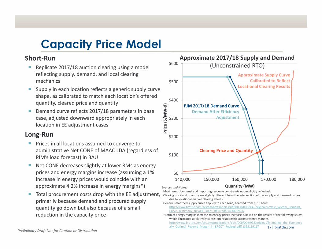
Capacity Price Model  Short‐Run

▀ Replicate 2017/18 auction clearing using a model reflecting supply, demand, and local clearing mechanics

▀ Supply in each location reflects a generic supply curve shape, as calibrated to match each location’s offered quantity, cleared price and quantity

▀ Demand curve reflects 2017/18 parameters in base case, adjusted downward appropriately in each location in EE adjustment cases

  Long‐Run▀ Prices in all locations assumed to converge to

administrative Net CONE of MAAC LDA (regardless of PJM’s load forecast) in BAU

▀ Net CONE decreases slightly at lower RMs as energy prices and energy margins increase (assuming a 1% increase in energy prices would coincide with an approximate 4.2% increase in energy margins*)

▀ Total procurement costs drop with the EE adjustment, primarily because demand and procured supply quantity go down but also because of a small reduction in the capacity price

Sources and Notes:Maximum sub‐annual and importing resource constraints not explicitly reflected.Clearing price and quantity are slightly different from the intersection of the supply and demand curves

due to locational market clearing effects.Generic smoothed supply curve applied to each zone, adapted from p. 15 here:

http://www.brattle.com/system/testimonies/pdfs/000/000/939/original/Brattle_System_Demand_Curve_Testimony_Newell_Spees_0414.pdf?1400682856

*Ratio of energy margins increase to energy prices increase is based on the results of the following study which illustrated a relatively consistent relationship across reserve margins: http://www.brattle.com/system/publications/pdfs/000/004/978/original/Estimating_the_Economically_Optimal_Reserve_Margin_in_ERCOT_Revised.pdf?1395159117

Approximate 2017/18 Supply and Demand(Unconstrained RTO)


$0

$20

$40

$60

$80

$100

$120

$140

$160

$180

0.8 1.0 1.2 1.4 1.6 1.8

Energy Price ($/M

Wh)

Local Reserve Margin

On‐Peak

Off‐ Peak

$0

$50

$100

$150

$200

$250

0.4 0.6 0.8 1.0 1.2 1.4

Energy Price ($/M

Wh)

Local Reserve Margin

On‐Peak

Off‐ Peak

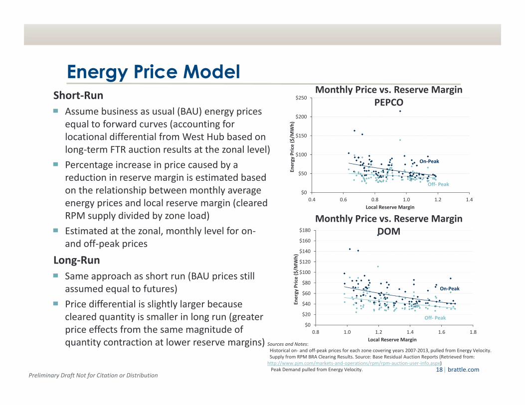
Energy Price Model  Short‐Run

▀ Assume business as usual (BAU) energy prices equal to forward curves (accounting for locational differential from West Hub based on long‐term FTR auction results at the zonal level)

▀ Percentage increase in price caused by a reduction in reserve margin is estimated based on the relationship between monthly average energy prices and local reserve margin (cleared RPM supply divided by zone load)

▀ Estimated at the zonal, monthly level for on‐and off‐peak prices

  Long‐Run

▀ Same approach as short run (BAU prices still assumed equal to futures)

▀ Price differential is slightly larger because cleared quantity is smaller in long run (greater price effects from the same magnitude of quantity contraction at lower reserve margins) Sources and Notes:

Historical on‐ and off‐peak prices for each zone covering years 2007‐2013, pulled from Energy Velocity.Supply from RPM BRA Clearing Results. Source: Base Residual Auction Reports (Retrieved from: http://www.pjm.com/markets‐and‐operations/rpm/rpm‐auction‐user‐info.aspx) Peak Demand pulled from Energy Velocity.

Monthly Price vs. Reserve Margin PEPCO

Monthly Price vs. Reserve Margin DOM


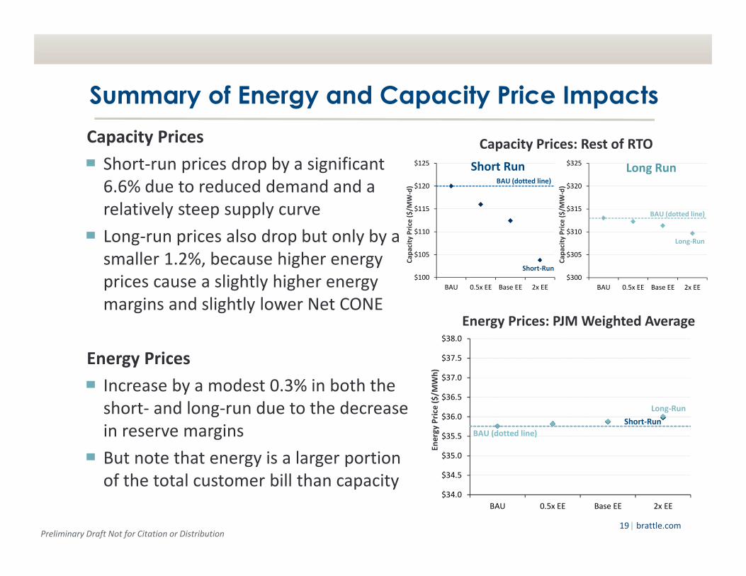
Summary of Energy and Capacity Price ImpactsCapacity Prices

▀ Short‐run prices drop by a significant 6.6% due to reduced demand and a relatively steep supply curve

▀ Long‐run prices also drop but only by a smaller 1.2%, because higher energy prices cause a slightly higher energy margins and slightly lower Net CONE

Energy Prices

▀ Increase by a modest 0.3% in both the short‐ and long‐run due to the decrease in reserve margins

▀ But note that energy is a larger portion of the total customer bill than capacity

Energy Prices: PJM Weighted Average

Capacity Prices: Rest of RTO

$34.0

$34.5

$35.0

$35.5

$36.0

$36.5

$37.0

$37.5

$38.0

BAU 0.5x EE Base EE 2x EE

Energy Price ($/M

Wh)

Long‐Run

Short‐Run

BAU (dotted line)

$100

$105

$110

$115

$120

$125


Cap

acity Price ($/M

W‐d)

Short‐Run

BAU (dotted line)

$300

$305

$310

$315

$320

$325


Cap

acity Price ($/M

W‐d)

Long‐Run

BAU (dotted line)

Short Run Long Run


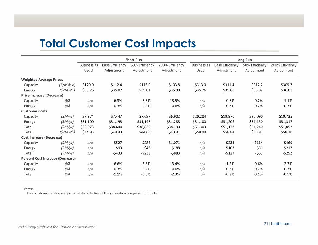
Summary of Total Customer Cost ImpactsBase Efficiency Adjustment

  Total customer costs are lower relative to the BAU, both in theshort and in the long run

▀ Total customer costs drop by $433M/yr in the short run and by$127M/yr in the long run

  The largest cost reduction comes from reduction in capacityprocurement costs

▀ $527M/yr in the short run and $233M/yr in the long run

  Energy costs increase slightly due to the decrease in reservemargins, but this does not change the direction of total costs

▀ $93M/yr in the short run and $107M/yr in the long run


Total Customer Cost Impacts

Notes:Total customer costs are approximately reflective of the generation component of the bill.

Short Run Long Run

Business as

Usual

Base Efficiency

Adjustment

50% Efficiency

Adjustment

200% Efficiency

Adjustment

Business as

Usual

Base Efficiency

Adjustment

50% Efficiency

Adjustment

200% Efficiency

Adjustment


Capacity ($/MW‐d) $120.0 $112.4 $116.0 $103.8 $313.0 $311.4 $312.2 $309.7

Energy ($/MWh) $35.76 $35.87 $35.81 $35.98 $35.76 $35.88 $35.82 $36.01


Capacity (%) n/a ‐6.3% ‐3.3% ‐13.5% n/a ‐0.5% ‐0.2% ‐1.1%

Energy (%) n/a 0.3% 0.2% 0.6% n/a 0.3% 0.2% 0.7%

Customer Costs

Capacity ($M/yr) $7,974 $7,447 $7,687 $6,902 $20,204 $19,970 $20,090 $19,735

Energy ($M/yr) $31,100 $31,193 $31,147 $31,288 $31,100 $31,206 $31,150 $31,317

Total ($M/yr) $39,073 $38,640 $38,835 $38,190 $51,303 $51,177 $51,240 $51,052

Total ($/MWh) $44.93 $44.43 $44.65 $43.91 $58.99 $58.84 $58.92 $58.70


Capacity ($M/yr) n/a ‐$527 ‐$286 ‐$1,071 n/a ‐$233 ‐$114 ‐$469

Energy ($M/yr) n/a $93 $48 $188 n/a $107 $51 $217

Total ($M/yr) n/a ‐$433 ‐$238 ‐$883 n/a ‐$127 ‐$63 ‐$252


Capacity (%) n/a ‐6.6% ‐3.6% ‐13.4% n/a ‐1.2% ‐0.6% ‐2.3%

Energy (%) n/a 0.3% 0.2% 0.6% n/a 0.3% 0.2% 0.7%

Total (%) n/a ‐1.1% ‐0.6% ‐2.3% n/a ‐0.2% ‐0.1% ‐0.5%


Study Caveats  EE Projections:

▀ Our study is not intended to substitute for a coordinated effort that might be led by PJM to project EE savings in the forecast period and account for them in the load forecasting effort. This study is an effort to gauge the magnitude of the EE missing from the load forecasts based on publicly available data sources and reasonable assumptions based on these data sources

  Capacity:

▀ Assumes short‐term supply would be totally unaffected by changes to administrative demand

▀ Short and long‐term effects do not account for effects of the 2.5% holdback, sub‐annual resource constraints, or maximum import constraints

▀ Long‐term effects assume all locations converge to the same Net CONE, and reflect a rough, approximate relationship between energy prices and energy margins but that was estimated for a different system


Study Caveats  Energy:

▀ BAU energy prices reflect forward curves current as of January 2014; forward curves have increased since that time

▀ “Long‐term” case for both energy and capacity is illustrative in magnitude relative to the 2017/18 delivery year but does not consider other factors that would change between then and a true long‐term equilibrium including other changes to supply, demand, fuel prices, etc.

  Other:

▀ This study does not account for the potential benefits of avoided transmission and distribution investments that would emerge from a more complete treatment of the EE impacts in the load forecasting process

▀ This study was completed before the issuance of proposed regulations pursuant to Section 111(d) of the Clean Air Act and therefore relied on the historical trends for projecting future EE. With the renewed emphasis on EE with Section 111(d), the future EE trends might be different from that of the historical period and yield larger amounts of EE than assumed in our analysis


Appendix 1Distinction between

Accounting for Projected EE vs.Implementing New EE


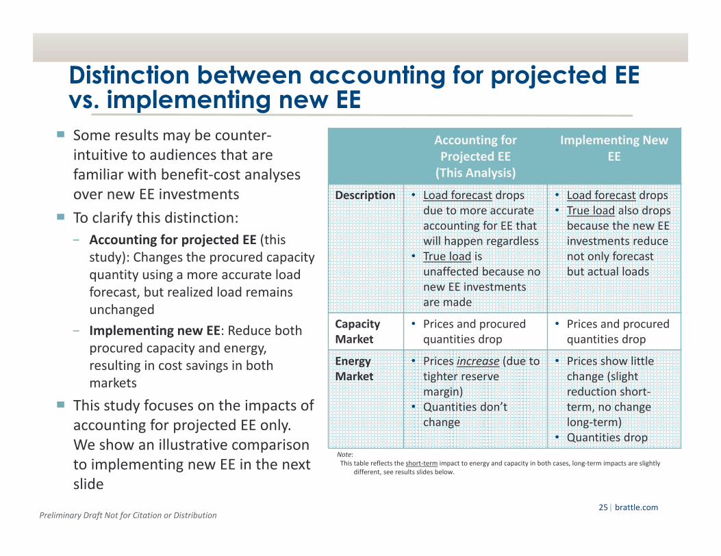
Distinction between accounting for projected EE vs. implementing new EE

▀ Some results may be counter‐intuitive to audiences that are familiar with benefit‐cost analyses over new EE investments

▀ To clarify this distinction:

− Accounting for projected EE (this study): Changes the procured capacity quantity using a more accurate load forecast, but realized load remains unchanged

− Implementing new EE: Reduce both procured capacity and energy, resulting in cost savings in both markets

▀ This study focuses on the impacts of accounting for projected EE only. We show an illustrative comparison to implementing new EE in the next slide

Accounting for Projected EE(This Analysis)

Implementing New EE

Description • Load forecast drops due to more accurate accounting for EE that will happen regardless

• True load is unaffected because no new EE investments are made

• Load forecast drops • True load also drops because the new EE investments reduce not only forecast but actual loads

Capacity Market

• Prices and procured quantities drop

• Prices and procured quantities drop

Energy Market

• Prices increase (due to tighter reserve margin)

• Quantities don’t change

• Prices show little change (slight reduction short‐term, no change long‐term)

• Quantities dropNote: This table reflects the short‐term impact to energy and capacity in both cases, long‐term impacts are slightly

different, see results slides below.


Cost Impacts: Accounting for Projected EE vs. Implementing New EE

Notes:Total customer costs are approximately reflective of the generation component of the bill.For the New EE Investments case: short‐run energy price decrease from BAU would be smaller if the EE adjustments were not concentrated in the highest priced zones. Long‐run energy price is slightly lower than in BAU, again because higher EE is observed in higher priced zones.

  For purposes of clarification, we compare here the price and cost impacts between the two cases: accounting for projected EE and implementing new EE Investments

Short Run Long Run

Business as

Usual

Forecast EE

Adjustment

New EE

Investments

Business as

Usual

Forecast EE

Adjustment

New EE

Investments


Capacity ($/MW‐d) $120.0 $112.4 $112.4 $313.0 $311.4 $313.0

Energy ($/MWh) $35.76 $35.87 $35.68 $35.76 $35.88 $35.75


Capacity (%) n/a ‐6.3% ‐6.3% n/a ‐0.5% 0.0%

Energy (%) n/a 0.3% ‐0.2% n/a 0.3% 0.0%

Customer Costs

Capacity ($M/yr) $7,974 $7,447 $7,447 $20,204 $19,970 $20,075

Energy ($M/yr) $31,100 $31,193 $30,829 $31,100 $31,206 $30,891

Total ($M/yr) $39,073 $38,640 $38,276 $51,303 $51,177 $50,966

Total ($/MWh) $44.93 $44.43 $44.29 $58.99 $58.84 $58.98


Capacity ($M/yr) n/a ‐$527 ‐$527 n/a ‐$233 ‐$129

Energy ($M/yr) n/a $93 ‐$271 n/a $107 ‐$208

Total ($M/yr) n/a ‐$433 ‐$797 n/a ‐$127 ‐$338


Capacity (%) n/a ‐6.6% ‐6.6% n/a ‐1.2% ‐0.6%

Energy (%) n/a 0.3% ‐0.9% n/a 0.3% ‐0.7%

Total (%) n/a ‐1.1% ‐2.0% n/a ‐0.2% ‐0.7%


Appendix 2Verification of the Study Approach

using the ISO-NE data


We applied our methodology to the ISO-NE data to gauge how closely it approximates ISO-NE EE Working Group’s projections

 We found that our approach has yielded missing EE projectionsthat are roughly half of the projections of the ISO‐NE’s EEWorking Group

  This implies that our projection approach is likely tounderestimate the level of new EE that will be implemented inthe forecast period. Therefore, our results are most likely to beon the conservative side


ISO-NE accounts for the projected EE in its load forecasts beyond the FCM time frame  Here, we apply our study methodology to the ISO‐NE data and compare the resulting load forecasts to those resulting from the ISO‐NE’s Energy Efficiency Working Group process

  ISO‐NE’s historical data is grossed up for historical energy efficiency savings, therefore there is only negligible amount of “embedded EE” in the forecasts

▀ No adjustment for double counting is needed

 We downloaded the EIA‐861 data on annual incremental EE savings for 2009‐2012 for each of the six New England states

 We assumed that new programs that would yield the same amount of “incremental “EE savings will be introduced each year through 2023


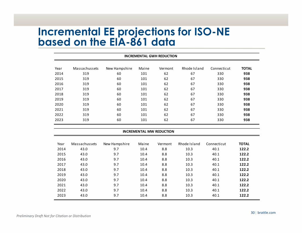
Incremental EE projections for ISO-NE based on the EIA-861 data

Year Massachussets New Hampshire Maine Vermont Rhode Island Connecticut TOTAL

2014 319 60 101 62 67 330 938

2015 319 60 101 62 67 330 938

2016 319 60 101 62 67 330 938

2017 319 60 101 62 67 330 938

2018 319 60 101 62 67 330 938

2019 319 60 101 62 67 330 938

2020 319 60 101 62 67 330 938

2021 319 60 101 62 67 330 938

2022 319 60 101 62 67 330 938

2023 319 60 101 62 67 330 938

INCREMENTAL GWH REDUCTION

Year Massachussets New Hampshire Maine Vermont Rhode Island Connecticut TOTAL

2014 43.0 9.7 10.4 8.8 10.3 40.1 122.2

2015 43.0 9.7 10.4 8.8 10.3 40.1 122.2

2016 43.0 9.7 10.4 8.8 10.3 40.1 122.2

2017 43.0 9.7 10.4 8.8 10.3 40.1 122.2

2018 43.0 9.7 10.4 8.8 10.3 40.1 122.2

2019 43.0 9.7 10.4 8.8 10.3 40.1 122.2

2020 43.0 9.7 10.4 8.8 10.3 40.1 122.2

2021 43.0 9.7 10.4 8.8 10.3 40.1 122.2

2022 43.0 9.7 10.4 8.8 10.3 40.1 122.2

2023 43.0 9.7 10.4 8.8 10.3 40.1 122.2

INCREMENTAL MW REDUCTION


Comparison Approach We first take ISO‐NE’s unrestricted load forecasts and create two restricted load forecasts:

▀ One using the EE that cleared in the FCM through 2017 and keeping it constant at the 2017 level for the remainder of the forecast period 2018‐2023

▀ Other using the EE cleared in the FCM through 2017 and using the ISO‐NE projected EE values for the remainder of the forecast period 2018‐2023

  Delta between the two restricted load forecasts yields the amount of EE that would go unaccounted for in the absence of ISO‐NE’s efforts to project EE beyond FCM

 Next, we repeat the same exercise, this time replacing the ISO‐NE projected EE values with the Brattle projected EE values using the EIA‐861 data


Using the ISO-NE EE projections, the delta between the two restricted forecasts is 1.2% for energy and 0.8% for peak in 2018

Year Unresricted Energy FCM Add'l EE FCM + EE Load-FCM-EE Load-FCM DeltaDelta (% of

unrestricted energy)

2014 138,390 8848 0 8,848 129,542 129,542 - 2015 140,430 9955 0 9,955 130,475 130,475 - 2016 142,335 10909 0 10,909 131,426 131,426 - 2017 143,985 11862 0 11,862 132,123 132,123 -

2018 145,385 11862 1764 13,626 131,759 133,523 1,764 1.2%2019 146,620 11862 1659 15,285 131,335 134,758 3,423 2020 147,830 11862 1559 16,844 130,986 135,968 4,982 2021 149,055 11862 1462 18,306 130,749 137,193 6,444 2022 150,295 11862 1373 19,679 130,616 138,433 7,817

2023 151,525 11862 1288 20,967 130,558 139,663 9,105 6.0%

Year Unresricted Peak FCM Add'l EE FCM + EE Peak-FCM-EE Peak-FCM DeltaDelta (% of


2014 28,165 1507 0 1,507 26,658 26,658 - 2015 28,615 1685 0 1,685 26,930 26,930 - 2016 29,130 1839 0 1,839 27,291 27,291 - 2017 29,610 2089 0 2,089 27,521 27,521 -

2018 30,005 2089 239 2,328 27,677 27,916 239 0.8%2019 30,335 2089 225 2,553 27,782 28,246 464 2020 30,675 2089 211 2,764 27,911 28,586 675 2021 30,990 2089 198 2,962 28,028 28,901 873 2022 31,315 2089 186 3,148 28,167 29,226 1,059

2023 31,620 2089 174 3,322 28,298 29,531 1,233 3.9%


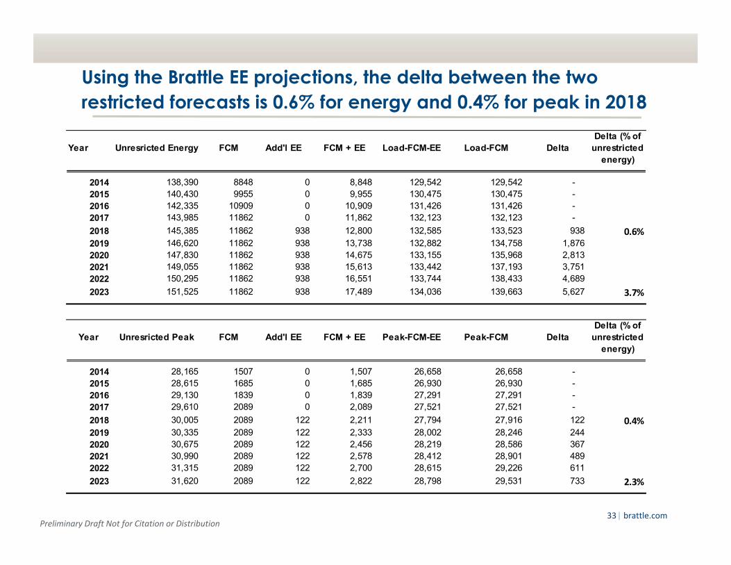
Using the Brattle EE projections, the delta between the two restricted forecasts is 0.6% for energy and 0.4% for peak in 2018

Year Unresricted Energy FCM Add'l EE FCM + EE Load-FCM-EE Load-FCM DeltaDelta (% of


2014 138,390 8848 0 8,848 129,542 129,542 - 2015 140,430 9955 0 9,955 130,475 130,475 - 2016 142,335 10909 0 10,909 131,426 131,426 - 2017 143,985 11862 0 11,862 132,123 132,123 -

2018 145,385 11862 938 12,800 132,585 133,523 938 0.6%2019 146,620 11862 938 13,738 132,882 134,758 1,876 2020 147,830 11862 938 14,675 133,155 135,968 2,813 2021 149,055 11862 938 15,613 133,442 137,193 3,751 2022 150,295 11862 938 16,551 133,744 138,433 4,689

2023 151,525 11862 938 17,489 134,036 139,663 5,627 3.7%

Year Unresricted Peak FCM Add'l EE FCM + EE Peak-FCM-EE Peak-FCM DeltaDelta (% of


2014 28,165 1507 0 1,507 26,658 26,658 - 2015 28,615 1685 0 1,685 26,930 26,930 - 2016 29,130 1839 0 1,839 27,291 27,291 - 2017 29,610 2089 0 2,089 27,521 27,521 -

2018 30,005 2089 122 2,211 27,794 27,916 122 0.4%2019 30,335 2089 122 2,333 28,002 28,246 244 2020 30,675 2089 122 2,456 28,219 28,586 367 2021 30,990 2089 122 2,578 28,412 28,901 489 2022 31,315 2089 122 2,700 28,615 29,226 611

2023 31,620 2089 122 2,822 28,798 29,531 733 2.3%


Findings of the Methodology Verification Using the ISO‐NE EE projections, the delta between the tworestricted forecasts is 1.2% (6%) for energy and 0.8% (3.9%) forpeak in 2018 (2023)

 Using the Brattle EE projections, the delta between the tworestricted forecasts is 0.6% (3.7%) for energy and 0.4% (2.3%)for peak in 2018 (2023)

  These results imply that our projection approach is likely tounderestimate the new EE that will be implemented in theforecast period. Therefore, our results are most likely to be onthe conservative side

Documents

Quantifying the Amount and Economic Impacts of …sustainableferc.org/wp-content/uploads/2014/09/Brattle...Quantifying the Amount and Economic Impacts of Missing Energy Efficiency