Embed Size (px)
Citation preview

Research Division Federal Reserve Bank of St. Louis Working Paper Series
Quantifying the Impact of Financial Development on Economic Development
Jeremy Greenwood Juan M. Sánchez
and Cheng Wang
Working Paper 2010-023C
http://research.stlouisfed.org/wp/2010/2010-023.pdf
August 2010 Revised April 2012
FEDERAL RESERVE BANK OF ST. LOUIS Research Division
P.O. Box 442 St. Louis, MO 63166
______________________________________________________________________________________
The views expressed are those of the individual authors and do not necessarily reflect official positions of the Federal Reserve Bank of St. Louis, the Federal Reserve System, or the Board of Governors.
Federal Reserve Bank of St. Louis Working Papers are preliminary materials circulated to stimulate discussion and critical comment. References in publications to Federal Reserve Bank of St. Louis Working Papers (other than an acknowledgment that the writer has had access to unpublished material) should be cleared with the author or authors.

Version: April 2012
Quantifying the Impact of Financial Development on Economic
Development
Jeremy Greenwood a, Juan M. Sanchez b;�, and Cheng Wang c; d
Abstract
How important is �nancial development for economic development? A costly state veri�cationmodel of �nancial intermediation is presented to address this question. The model is calibratedto match facts about the U.S. economy, such as the intermediation spreads and the �rm-sizedistributions for 1974 and 2004. It is then used to study the international data using cross-countryinterest-rate spreads and per-capita GDPs. The analysis suggests a country like Uganda couldincrease its output by 116 percent if it could adopt the world�s best practice in the �nancial sector.Still, this amounts to only 29 percent of the gap between Uganda�s potential and actual output.
Review of Economic Dynamics, forthcoming, special issue on �Misallocation and Productivity,�edited by Diego Restuccia and Richard Rogerson.
Keywords: costly state veri�cation, economic development, �nancial intermediation, �rm-size dis-tribution, interest-rate spreads, cross-country output di¤erences, cross-country di¤erences in �nan-cial sector productivity, cross-country TFP di¤erences
JEL Nos: E13, O11, O16
A iations:
a Department of Economics, University of Pennsylvania, McNeil Bldg. Rm 160, Philadelphia, PA19104-6927, USAb Research Division, Federal Reserve Bank of St. Louis, P.O. Box 442, St. Louis, MO 63166-0442,USAc School of Economics, Fudan University, Shanghai, China 200433d Department of Economics, Iowa State University, 260 Heady Hall, Ames, IA 50011-1070, USA
�Corresponding author at: Research Division, Federal Reserve Bank of St. Louis, P.O. Box 442, St.Louis, MO 63166-0442, USA. Email address: [email protected] (Juan M Sanchez). Phone:(314) 444-8564. Fax: (314) 444-8731.

1 Introduction
How important is �nancial development for economic development? Ever since the publi-
cation of Raymond W. Goldsmith�s (1969) classic book Financial Structure and Economic
Development, economists have been developing theories and searching for empirical evi-
dence connecting economic and �nancial development. Goldsmith emphasized the role that
intermediaries play in steering funds to the highest-valued users in the economy. First, in-
termediaries collect and analyze information before they invest in businesses. Based on this
information, they determine whether to commit savers�funds. If they proceed, then they
must decide how much to invest and on what terms. Second, after allocating funds inter-
mediaries must monitor �rms to ensure that savers�best interests are protected. Increases
in the e¢ ciency of �nancial intermediation, due to improved information production, are
likely to reduce the spreads between the internal rates of return on investments in �rms and
the rate of return on savings received by savers. The spreads between these returns re�ect
the costs of intermediation. These intermediation wedges include the costs of gathering ex
ante information about investment projects, the ex post information costs of policing invest-
ments, and the costs of misappropriation of savers�funds by management, unions, and so on
that arise in a world with imperfect information. An improvement in �nancial intermedia-
tion does not necessarily a¤ect the rate of return earned by savers. Aggregate savings may
adjust in equilibrium so that this return always equals savers�rate of time preference.
The left panel of Figure 1 plots the intermediation wedge for the U.S. economy over
time. (All data de�nitions are presented in the appendix.) The United States is a developed
economy with a sophisticated �nancial system. The wedge falls only slightly. At the same
time, it is di¢ cult to detect an upward trend in the capital-to-output ratio. Contrast this
with Taiwan (shown in the right panel): There is a dramatic drop in the interest-rate spread.
As the cost of capital falls, one would expect to see a rise in investment. Indeed, the capital-
to-output ratio for Taiwan shows a signi�cant increase. The observation that there is only a
small drop in the U.S. interest-rate spread does not imply that there has been no technological
advance in the U.S. �nancial sector. Rather, it may re�ect the fact that e¢ ciency in the
1
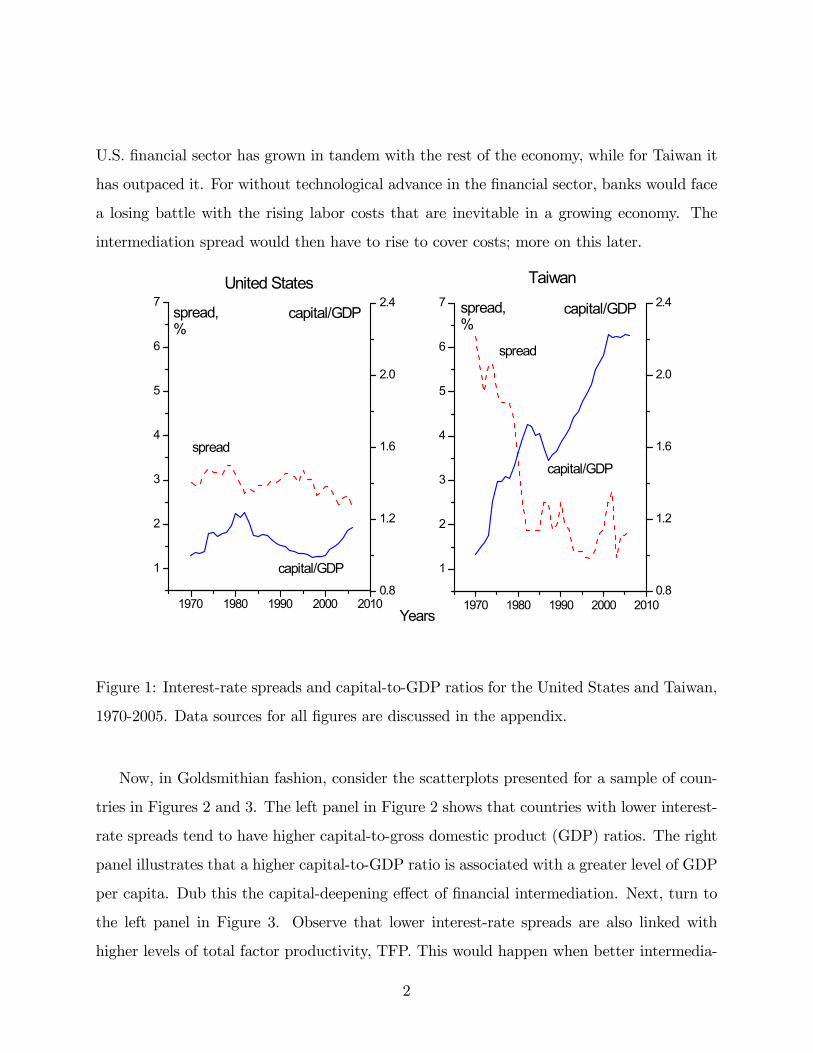
U.S. �nancial sector has grown in tandem with the rest of the economy, while for Taiwan it
has outpaced it. For without technological advance in the �nancial sector, banks would face
a losing battle with the rising labor costs that are inevitable in a growing economy. The
intermediation spread would then have to rise to cover costs; more on this later.
1970 1980 1990 2000 2010
1
2
3
4
5
6
7
0.8
1.2
1.6
2.0
2.4
1970 1980 1990 2000 2010
1
2
3
4
5
6
7
0.8
1.2
1.6
2.0
2.4
capital/GDP
spread
Taiwan
Years
spread,%
capital/GDP
capital/GDP
spread
United States
spread,%
capital/GDP
Figure 1: Interest-rate spreads and capital-to-GDP ratios for the United States and Taiwan,
1970-2005. Data sources for all �gures are discussed in the appendix.
Now, in Goldsmithian fashion, consider the scatterplots presented for a sample of coun-
tries in Figures 2 and 3. The left panel in Figure 2 shows that countries with lower interest-
rate spreads tend to have higher capital-to-gross domestic product (GDP) ratios. The right
panel illustrates that a higher capital-to-GDP ratio is associated with a greater level of GDP
per capita. Dub this the capital-deepening e¤ect of �nancial intermediation. Next, turn to
the left panel in Figure 3. Observe that lower interest-rate spreads are also linked with
higher levels of total factor productivity, TFP. This would happen when better intermedia-
2

tion tends to redirect funds to the more e¢ cient �rms. The right panel displays how higher
levels of TFP are connected with larger per-capita GDP. Call this the reallocation e¤ect
arising from �nancial intermediation. The capital deepening and reallocation e¤ects from
improved intermediation play an important role in what follows. While the above facts are
stylized, to be sure, empirical researchers have used increasingly sophisticated methods to
tease out the relationship between �nancial intermediation and growth. This literature is
surveyed masterfully by Levine (2005). An early example of the empirical research examin-
ing the link between �nancial intermediation and growth is the well-known paper by King
and Levine (1993). The upshot is that �nancial development has a causal e¤ect on economic
development; speci�cally, �nancial development leads to higher rates of growth in income
and productivity.
The impact of �nancial development on economic development is investigated here, quan-
titatively, using a costly state veri�cation model that was developed by Greenwood et al.
(2010). The source of inspiration for the framework is the classic work by Townsend (1979)
and Williamson (1986). It has two novel twists, however. First, �rms monitor cash �ows
as in Townsend (1979) and Williamson (1986); however, here the e¢ ciency of this activity
depends on both the amount of resources devoted to it and the productivity of the moni-
toring technology used in the �nancial sector. Second, �rms have ex ante di¤erences in the
structure of returns that they o¤er. A �nancial theory of �rm size emerges. At any point
in time, �rms o¤ering high expected returns are underfunded (relative to a world without
informational frictions), whereas others yielding low expected returns are overfunded. This
results from diminishing returns in information production. As the e¢ ciency of the �nancial
sector rises (relative to the rest of the economy), funds are redirected away from less produc-
tive �rms in the economy toward more productive ones. Furthermore, as the interest-rate
spread declines and the cost of borrowing falls, capital deepening occurs in the economy.
The model is calibrated to match some stylized facts for the U.S. economy, speci�cally
the �rm-size distributions and interest-rate spreads for the years 1974 and 2004. It replicates
these facts very well. The improvement in �nancial sector productivity required to duplicate
3

LUX
IRL
AUS
FIN
JPNCHE
NLDBEL
THA
PRT
NORAUT
ISRSWE
MUS
FRA
ETH
INDPAN
ITAESPDNK
MARBOL
PHLCOL
MEXURY
PER
NICKEN
HND
GTMNGA
UGA
BRA
TUR
ZAF
GBR
LKA
CRISLV
USA
NZLLUX
IRL
AUS
FIN
JPNCHE
NLDBEL
THA
PRT
NORAUT
ISRSWE
MUS
FRA
ETH
INDPAN
ITAESP DNK
MARBOL
PHLCOL
MEXURY
PER
NICKEN
HND
GTMNGA
UGA
BRA
TUR
ZAF
GBR
LKA
CRISLV
USA
NZL
0.00 0.05 0.10 0.150
1
2
3
4
Interestrate spread
Capit
al/GD
P ra
tio
0 10 20 30 40 500
1
2
3
4
Capit
al/GD
P ra
tio
GDP per capita, $ thousands
Figure 2: The cross-country relationship among interest-rate spreads, capital-to-GDP ratios
and GDPs per capita. The three letter country codes are taken from the International
Organization for Standardization, ISPO 3166-1 alpha-3.
these facts also appears to be reasonable; it does this with little change in the capital-to-
output ratio. In the model, improvements in �nancial intermediation account for 29 percent
of U.S. growth. The framework also is capable of mimicking the striking decline in the
Taiwanese interest-rate spread. At the same time, it predicts a signi�cant rise in the capital-
to-output ratio. It is estimated that dramatic improvements in Taiwan�s �nancial sector
accounted for 45 percent of the country�s economic growth.
The calibrated model is then applied to the cross-country data. It performs reasonably
well in predicting the di¤erences in cross-country capital-to-output ratios. Similarly, it does
a good job of matching the empirical relationship between �nancial development and average
4

ETHUGANGA
KEN
HNDPAKIND BOL NICPHL
GTM
MARLKA PER
EGYSLV
TURCOL
THA
BRAVENMEXPAN
CRIZAFURY
ARGTTO
MUS
PRT
ESPNZL
ISR
FIN
ITA
JPN
BEL
IRL
GBRFRASWE
NLDAUSCANAUT
DNKCHE
NOR
USA
LUX
ETHUGANGAKEN
HNDPAKINDBOLNICPHL
GTM
MARLKAPER
EGYSLVTURCOL
THA
BRAVENMEXPAN
CRIZAFURYARGTTO
MUS
PRT
ESPNZL
ISR
FIN
ITA
JPN
BEL
IRL
GBRFRASWE
NLDAUSCANAUTDNKCHE
NOR
USA
LUX
0.00 0.05 0.10 0.150
500
1000
1500
Interestrate spread
TFP
0 10 20 30 40 500
500
1000
1500
TFP
TFP
GDP per capita, $ thousands
Figure 3: The cross-country relationship among interest-rate spreads, TFPs and GDPs per
capita.
5

�rm size. Financial intermediation turns out to be important quantitatively. For example,
in the baseline model Uganda would increase its per-capita GDP by 116 percent if it could
somehow adopt Luxembourg�s �nancial system. World output would rise by 53 percent if
all countries adopted Luxembourg�s �nancial practice. Still, the bulk (or 69 percent) of
cross-country variation in per-capita GDP cannot be accounted for by variation in �nancial
systems.
Other researchers have recently investigated the relationship between �nance and devel-
opment that use quantitative models. The frameworks used, and the questions addressed,
di¤er from the current analysis. For example, Townsend and Ueda (2010) estimate a ver-
sion of the Greenwood and Jovanovic (1990) model to examine Thai �nancial reform. Their
analysis stresses the role of �nancial intermediaries in producing ex ante information about
the state of the economy at the aggregate level. Financial intermediaries o¤er savers higher
and safer returns. Townsend and Ueda (2010) �nd that Thai welfare increased about 15
percent due to �nancial liberalization.
Limited investor protection is emphasized by Castro et al. (2009). They build a two-
sector model to explain the positive cross-country correlation between investment and GDP.
They note that the capital-goods sector is risky. This risk makes capital goods expensive
to produce in poor countries with limited investor protection because of high �nance costs.
An implication of their framework is that the correlation between investment and GDP is
weaker when measured at domestic vis-à-vis international prices. This is true in the data. A
close cousin to the notion of limited investor protection is the idea of limited enforceability of
contracts. Buera et al. (2011) focus on the importance of limited enforceability of contracts
in distorting the allocation of entrepreneurial talent in the economy. This helps explain TFP
di¤erentials across nations. The interplay between the enforceability of contracts and the
allocation of managerial talent for explaining cross-country productivity di¤erences is also
investigated by Erosa and Cabrillana (2008) in a similar framework, albeit with more of a
theoretical emphasis. Finally, Midrigan and Xu (2010) challenge the view that the borrowing
constraints induced by limited enforceability of contracts create large reallocation e¤ects via
6
the distortion of factor inputs across �rms. They argue that �rms can quickly grow out of
the implied borrowing constraints.1
2 The economy
The analysis focuses on two types of agents: �rms and �nancial intermediaries. Firms pro-
duce output using capital and labor. Their production processes are subject to idiosyncratic
productivity shocks. The realized value of the productivity shock is a �rm�s private informa-
tion. All funding for capital must be raised from �nancial intermediaries. This is done before
the technology shock is observed. After seeing its shock, a �rm hires labor on a spot market.
When �nancing its capital a �rm enters into a �nancial contract with an intermediary. This
contract speci�es the state-contingent payment that a �rm must make to an intermediary
on completing production. Hidden in the background are consumers/workers, who supply a
�xed amount of labor to the economy. They also deposit funds with an intermediary that
earn a �xed rate of return. Given the focus here on comparative steady states, an analysis
of consumers/workers can be safely suppressed. The behavior of �rms and intermediaries is
described below in more detail.
2.1 Firms
Firms hire capital, k, and labor, l, to produce output, o, in line with the constant-returns-
to-scale production function
o = x�k�l1��:
The productivity level of a �rm�s production process is represented by x�. It is the product
of two components: an aggregate one, x, and an idiosyncratic one, �. The idiosyncratic level
of productivity is a random variable. Speci�cally, the realized value of � is drawn from the
two-point set � = f�1; �2g, with �1 < �2. The set � di¤ers across �rms. Call this the �rm�s
1 Additionally, dynamic contracts can potentially be used to mitigate such �nancial frictions. See Coleet al. (2012) for an analysis of technological adoption across countries using a framework with dynamiccontracts for �rm �nance.
7

type. Let Pr(� = �1) = �1 and Pr(� = �2) = �2 = 1� �1. The probabilities for the low and
high states (1 and 2, respectively) are the same across �rms. The realized value of � 2 � is
a �rm�s private information. For now take the aggregate level of productivity, x, to be some
known constant.
Suppose that a type-� �rm has raised k units of capital. It then draws the productivity
shock �i. It must now decide how much labor, li, to hire at the wage rate w. In other words,
the �rm solves the maximization problem shown below.
R(�i; w)k � maxlifx�ik�l1��i � wlig: P(1)
Denote the optimal amount of labor that a type-� �rm will hire in state i by li(�) = li(�1; �2).
Substituting the implied solution for li into the maximand and solving yields the unit return
function, R(�i; w), or
ri(�) � R(�i; w) = �(1� �)(1��)=�w�(1��)=�(x�i)1=� > 0: (1)
Think about ri(�) = R(�i; w) as giving the gross rate of return on a unit of capital invested
in a type-� �rm, given that state �i occurs. Finally, represent the amount of output that a
type-� �rm will produce in state i by
oi(�) = oi(�1; �2) = x�ik(�1; �2)�li(�1; �2)
1��;
where k(�) = k(�1; �2) is the size of the loan that will be received by this �rm. The next
section discusses how this loan is determined.
2.2 Financial intermediaries
Intermediation is competitive. Intermediaries raise funds from consumers and lend them to
�rms. Even though an intermediary knows a �rm�s type, � , it cannot observe the state of
a �rm�s business either costlessly or perfectly. That is, the intermediary cannot costlessly
observe �, o, and l. Suppose a �rm�s true productivity in a period is �i. It reports to
the intermediary that its productivity is �j, which may di¤er from �i. The intermediary
8

can audit this report. It seems reasonable to presume that the odds of detecting fraud are
increasing in the amount of labor devoted to verifying the claim, lmj, decreasing in the size
of the loan, k (because there will be more activity to monitor), and rising in the productivity
of the monitoring technology, z.
Let Pij(lmj; k; z) denote the probability that the �rm is caught cheating conditional on
the following: (1) the true realization of productivity is �i; (2) the �rm makes a report of
�j; (3) the intermediary allocates lmj units of labor to monitor the claim; (4) the size of
the loan is k (which represents the scale of the project); (5) the level of productivity in the
monitoring activity is z. The function Pij(lmj; k; z) is increasing in lmj and z and decreasing
in k. Additionally, let Pij(lmj; k; z) = 0 if the �rm truthfully reports that its type is �i (i.e.,
when j = i). A convenient formulation for Pij(lmj; k; z) is2
Pij(lmj; k; z) =
8>>><>>>:1� 1
�(z=k) (lmj) < 1; with 0 < < < 1;
for a report �j 6= �i;
0; for a report �j = �i:
(2)
Suppose that loan size, k, increases. Let the intermediary raise the amount of labor, lmj,
that it will use to monitor a claim of state j by the same proportion. Observe that the odds
of detecting malfeasance, Pij(lmj; k; z), will fall (for a report of �j 6= �i) because < . In
this sense, there are diminishing returns to scale in monitoring.
The intermediary gives a �rm a loan of size k. In exchange for providing the loan the
intermediary collects some speci�ed state-contingent payments from the �rm. The rents
that accrue to a �rm depend on the true state of its technology, �i, the state that it reports,
�j, plus the outcome of any monitoring that is done. Clearly, a �rm will have no incentive
to misreport when the bad state, �1, occurs. Similarly, the intermediary will never monitor
a good report, �j = �2; it will audit only bad ones, �j = �1. If it �nds malfeasance, then
2 To guarantee that Pij(lmj ; k; z) � 0 this speci�cation requires, when �j 6= �i, that some minimal levelof labor must be devoted to monitoring; that is, lmj > ��1= (k=z)
� == . Note that this minimal labor
requirement for monitoring can be made arbitrarily small by picking a large enough value for ". The choiceof " can be thought of as normalization relative to the level of productivity in the production of monitoringservices; see Greenwood et al. (2010) for more detail.
9

the intermediary should exert maximal punishment, which amounts to seizing everything or
r2k. If it does not, then it should take all of the bad state returns, or r1k. These latter two
features help to create, in a least-cost manner, an incentive for the �rm to tell the truth. The
above features are embedded in the contracting problem presented below. A more formal,
step-by-step analysis is presented in Greenwood et al. (2010).
Turn now to the contracting problem. Intermediation is competitive. Therefore, an
intermediary must choose the details of the �nancial contract to maximize the expected
rents for a �rm. Otherwise, the �rm will take out a loan elsewhere. Competition implies
that all intermediaries earn zero pro�ts on their lending activity. Suppose that intermediaries
can raise funds from savers at the interest rate br. If the depreciation rate on physical capitalis �, then the cost of supplying capital is er = br+�. The intermediary�s optimization problemcan be expressed as3
v � maxk;lm1
f�2[1� P21(lm1; k; z)][r2(�)� r1(�)]kg; P(2)
subject to
[�1r1(�) + �2r2(�)]k � �2[1� P21(lm1; k; z)][r2(�)� r1(�)]k � �1wlm1 � erk = 0: (3)
The objective function P(2) gives the expected rents for a �rm. These rents accrue from
the fact that the �rm has private information about its state. Suppose that the �rm lies
about being in the good state. When it does not get caught, it can pocket the amount
[r2(�)� r1(�)]k. The odds of not getting caught are 1�P21(lm1; k; z). The good state occurs
with probability �2. An incentive-compatible contract o¤ers the �rm the same amount
for telling the truth that it can get by lying.4 Equation (3) is the intermediary�s zero-
pro�t condition. The expected return from the project is [�1r1(�) + �2r2(�)]k. Out of
3 This is the dual of the problem presented in Greenwood et al. (2010).
4 Let p2 represent the payment that a �rm makes to the intermediary in the good state. The incentiveconstraint for the contract will read
[1� P21(lm1 ; k; z)][r2(�)� r1(�)]k � r2(�)k � p2:
The left-hand side of this equation represents what the �rm will obtain by lying, while the right-hand sideshows what it will receive when it tells the truth. The latter must dominate, in a weak sense, the former.
10

this amount the intermediary must give the �rm �2[1 � P21(lm1; k; z)][r2(�) � r1(�)]k. The
expected cost of monitoring low-state returns is �1wlm1. The cost of supplying the capital
is erk. Represent the optimal amount of labor required to monitor a type-� �rm in state
1 by lm1(�) = lm1(�1; �2). The contract presumes that the intermediary is committed to
monitoring all reports of a bad state. Likewise, denote the quantity of capital that is lent
to a type-� �rm by k(�) = k(�1; �2). Finally, for some types of �rms a loan may entail a
loss; the intermediary will not lend to these �rms.
2.3 Stationary equilibrium
The focus of the analysis is solely on stationary equilibria. Firms di¤er by type, � = (�1; �2)
with �1 < �2. Denote the space of types by T � R2+. Suppose that �rms are distributed
over productivities in accordance with the distribution function
F (x; y) = Pr(�1 � x; �2 � y).
For all �rms �x the odds of drawing state i at Pr(� = �1) = �i. This distribution F can then
be thought of as specifying the mean, �1�1 + �2�2, and variance, �1�2(�1 � �2)2, of project
returns across �rms. So, which �rms will receive funding in equilibrium?
To answer this question, focus on the zero-pro�t condition for intermediaries (3). Now
consider a �rm of type � . Clearly, if �1r1(�)k + �2r2(�)k � erk < 0, then the intermediary
will incur a loss on any loan of size k > 0. Likewise, if �1r1k+�2r2k�erk > 0, then it will bepossible to make non-negative pro�ts, albeit the loan may have to be very small. Therefore,
a necessary and su¢ cient condition to obtain funding is that � lies in the set A(w) � T
de�ned by
A(w) � f� : �1r1(�) + �2r2(�)� er > 0g: (4)
(Recall that upon the declaration of a bad state, the �rm must turn over r1(�)k to the intermediary. So, itwill make nothing when it truthfully reports a bad state. If the �rm gets caught cheating, then it must makethe payment r2(�)k, so it will also earn zero rents here.) The incentive constraint will bind. Thus, P(2)maximizes the �rm�s expected rents, �2[r2(�)k � p2], subject to the zero-pro�t constraint. As in Townsend(1979), it can be shown that the revelation principle holds, so the focus here on incentive-compatible contractsis without loss of generality.
11
This set shrinks with the wage, w, because ri(�) is decreasing in w; as wages rise, a �rm
becomes less pro�table.
Firms with � 2 A(w) will demand li(�1; �2) units of labor in state i. Should one of these
�rms declare that it is in state 1, then the intermediary will send lm1(�1; �2) units of labor
to audit it. Recall that labor is in �xed supply. Suppose there is one unit in aggregate. The
labor-market-clearing condition will then appear asZA(w)
[�1l1(�1; �2) + �2l2(�1; �2) + �1lm1(�1; �2)]dF (�1; �2) = 1. (5)
It is now time to take stock of the situation thus far by presenting a de�nition of the
equilibrium under study.
De�nition 1 Set the steady-state cost of capital at er. A stationary competitive equilibriumis described by a set of labor allocations, li and lm1, a loan size, k, and a value, v, for each�rm, a set of active �rms, A(w), and a wage rate, w, such that:
1. The loan, k, o¤ered by the intermediary maximizes the value of a �rm, v, in line withP(2), given the prices er and w. The intermediary hires labor for monitoring in theamount lm1, as also speci�ed by P(2).
2. A �rm is o¤ered a loan if and only if it lies in the active set, A(w), as de�ned byequation (4).
3. A �rm hires labor, li, to maximize its pro�ts in accordance with P(1), given wages, w,and the size of the loan, k, o¤ered by the intermediary.
4. The wage rate, w, is determined so that the labor market clears, in accordance with(5).
3 Discussion
The analysis focuses on the role that intermediaries play in producing information. Before
an investment opportunity is funded, intermediaries assess its risk and return. In the current
setting, this amounts to knowing a project�s type, � . This can be costlessly discovered in
the model here. It would be easy to add a variable cost for a loan that is a function of z.5
Doing so would have little bene�t in the current context, however.
5 One could think about � as representing the activity, industry, or sector within which a �rm operates.For instance, Castro et al. (2009, Figure 3) present data suggesting that the capital-goods sector is riskier
12

Intermediaries need to have systems in place to monitor cash �ows or face the prospect
of lower-than-promised returns. This is true regardless of whether investment funds are
internally or externally generated. In times past, banks required borrowers to keep their
funds in an account with them so that transactions could be monitored. Even a privately
funded �rm needs to be monitored, unless the scale is so small that the owner can operate
it himself. Family-owned �rms may mitigate the monitoring problem and are prevalent
in poorer countries; see Caselli and Gennaioli (forthcoming) for a model of family-owned
enterprises.
Managers and workers tend to siphon funds from the providers of capital, regardless of
whether they are banks, bondholders, private owners, shareholders, or venture capitalists.
At the micro level, this is what a shirking worker in a fast-food restaurant does. Computer
surveillance software, called HyperActive Bob, designed to catch such a person is available
from HyperActive Technologies for $200 a month.6 In a dynamic contracting setting, with
monitoring, it may appear at some points in time that the �rm is relying heavily on internally
generated funds to �nance investments. This is especially true for older �rms. Yet starting
the �rm may have required funding from outside investors. Without the ability to monitor
cash �ows, investors may �nd that projects that require large upfront funds for payo¤s that
occur far in the future may deliver very disappointing returns. In fact, starting such a
venture may not be feasible if investors cannot monitor the cash �ows during the critical
stages of the enterprise�s developmen; see Cole et al. (2012) for an example. Measures of
external �nancing also survey �rms relatively late in their growth cycle. They do not capture
the fact that start-ups use capital from private investors, such as venture capitalists.
The e¢ ciency of monitoring, z, is likely to depend on the state of technology in the �-
nancial sector, both in terms of human and physical capital. Better information technologies
than the consumption-goods one. As just discussed, it would be possible to have a screening stage wherethe intermediary veri�es the initial type of a �rm. It may not be possible to detect perfectly a �rm�s type.Even so, it may be feasible to design a contract that will reveal it. The ability to screen, albeit imperfectly,may play an important role in designing such a contract. See the classic paper by Boyd and Prescott (1986)for such an approach.
6 �Machines that can see.�The Economist, March 5, 2009.
13

allow for larger quantities of �nancial information to be collected, exchanged, processed, and
analyzed. Indeed, the most information technology intensive industry in the United States
is Depository and Nondepository Financial Institutions. Computer equipment and software
services accounted for 10 percent of value added over the period 1995 to 2000, as opposed
to 5 percent in Industrial Machinery and Equipment, or 2.6 percent in Radio and Television
Broadcasting. Berger (2003) discusses the importance of IT in accounting for productivity
gains in the U.S. banking sector. This is re�ected in the growth of automated teller ma-
chines, Internet banking, electronic payment technologies, and information exchanges that
permit the use of economic models to undertake credit scoring for small businesses, develop
investment strategies, create new exotic �nancial products, etc. Similarly, a more talented
workforce allows for higher-quality information workers: accountants, �nancial analysts, and
lawyers. Last, the e¢ ciency of monitoring depends on the legal environment, which speci�es
what information can, must, or must not be produced. This factor is separate from regu-
lating the terms of payments, especially in bankruptcy as analyzed in Castro et al. (2009).
That is, in the current setting, a �rm must pay the amount r1k in the low state, but one
could imagine that limited investor protection might reduce this to some smaller amount.
Before proceeding to the quantitative analysis, some mechanics of the above framework
are inspected in a heuristic manner; for a more formal analysis, see Greenwood et al. (2010).
The presence of diminishing returns to information production leads to a �nancial theory of
�rm size, as will be discussed. In fact, the diminishing returns to information production can
be thought of as providing a microfoundation for the Lucas (1978) span of control model.
The framework also speci�es a link between the state of �nancial development and the state
of economic development. Some of the mechanics are detailed now.
1. A �rm�s production is governed by constant returns to scale. In the absence of �nancial
market frictions, no rents would be earned on production. Additionally, in a frictionless
world only �rms o¤ering the highest expected return would be funded. In this situation,
max�2T [�1r1(�)+�2r2(�)] = er� cf (4). With �nancial market frictions, �1r1(�)+�2r2(�) > erfor all funded projects � 2 A(w), a fact easily gleaned from equation (3). Thus, deserving
14

projects� those � 2 B(w) � fx : maxx2T [�1r1(x) + �2r2(x)]g� will be underfunded, while
undeserving projects� � =2 B(w)� are simultaneously overfunded. Funded �rms will earn
rents, v, as given by P(2).
2. What determines the size of a �rm�s loan? By glancing at the left-hand side of
equation (3), which details the intermediary�s pro�ts, it looks likely that the �rm�s loan will
be increasing in the project�s expected return, �1r1(�)+�2r2(�), ceteris paribus. This is true:
Recall that the odds of detecting fraud, P21(lm1; k; z), decrease in loan size, k. Therefore,
more labor must be allocated to monitor the project in response to an increase in loan size.
Similarly, a �rm�s loan will decrease in the project�s risk, as measured by r2(�) � r1(�);
note that the variance in returns for a type-� �rm is given by �1�2[r2(�) � r1(�)]2. When
the spread between the high and low states widens, the incentive is stronger for the �rm to
misreport its returns. Recall that the gain from lying is given by the objective function in
P(2). To counter this the intermediary must devote more labor to monitoring. Diminishing
returns to information production imply that loan size, k, is uniquely speci�ed as a function
of expected return, �1r1(�) + �2r2(�), and risk, r2(�)� r1(�).
3. Imagine that aggregate productivity, x, grows over time at the constant rate g1=�
and let �nancial sector productivity, z, improve at the �xed rate g. Will there be balanced
growth? Conjecture that along a balanced growth path the k�s, o�s, and w will all grow
at rate g. Also guess that A(w) and the li�s, lm1�s, and ri(�)�s will remain constant. This
conjectured solution is veri�ed in a heuristic manner. It is easy to see from the isoelastic
forms of problem P(1) and equation (1) that the conjectured solution for balanced growth
path will be satis�ed for the li�s and ri(�)�s. Since the ri(�)�s remain constant so does the
active set, A(w), which is spelled out in (4). What about the k�s and the lm1�s? The solution
guessed for k and lm1 is consistent with P(2), if P21 does not change along a balanced growth
path. From equation (2) it is clear that the odds of getting caught cheating, P21, will change
over time, however, unless z grows at precisely the rate g. This is assumed, though. Since
the li�s and lm1�s remain �xed, if the labor-market clearing condition (5) holds at one point
along the balanced path it will hold at all others. Thus, the hypothesized solution for w is
15

consistent with labor-market clearing. Thus, the conjectured solution for balanced growth
occurs.
4. Consider the case where x grows at a di¤erent rate than z. Speci�cally, for illustrative
purposes, take the extreme situation where z rises while x remains �xed. Thus, there is only
�nancial innovation in the economy. According to (2) the odds of detecting fraud will rise,
other things equal. The rents that �rms accrue will drop, a fact that is evident from the
objective function in P(2). This makes it feasible for �nancial intermediaries to o¤er �rms
larger loans, ceteris paribus, as can be gleaned from equation (3). The implied increase in the
economy�s aggregate capital stock will then drive up wages. Thus, ine¢ cient �rms will have
their funding cut, as (4) makes clear. The active set of �rms, A(w), thus shrinks. Therefore,
�nancial innovation operates to cull unproductive �rms. Average �rm size in the economy is
the total stock of labor (1) divided by the number of �rms (or the measure of the active set).
Therefore, average �rm size increases. (The last two statements ignore the small amount of
labor used in monitoring.) If z increases without bound, then the economy will enter into
a frictionless world where only �rms o¤ering the highest expected return, max� [�1r1(�) +
�2r2(�)], are funded. These �rms will earn no rents; that is, max�2T [�1r1(�) + �2r2(�)] = er.4 The United States and Taiwan
The quantitative analysis will now begin. To simulate the model, values must be assigned to
its parameters. In a nutshell, these parameter values are based solely on information about
the U.S. economy, with two exceptions. The U.S. information is from either the literature or
stylized facts about the U.S. establishment-size distribution. The exceptions are the country-
speci�c levels of productivity in the production and �nancial sectors, or x and z. These two
variables are chosen so that the model matches a country�s income and its spread between
borrowing and lending rates. It is obvious that the level of TFP in a country, x, is tightly
linked with its income. The spread between borrowing and lending rates re�ects the costs of
intermediation, at least in worlds where intermediation services are competitively provided.
Thus, the interest-rate spread is connected to the level of e¢ ciency in the �nancial sector,
16

or z. So, the simulations will use a common set of parameter values for all countries, but
for x and z. The U.S., Taiwan, and later, 45 other countries each have their own levels of
productivity for the production and �nancial sectors, or their own x�s and z�s.
4.1 Fitting the model to the U.S. economy
Some parameters are standard and thus can be chosen on the basis of a priori information.
They are given conventional values. Capital�s share of income, �, is chosen to be 0:35, a very
standard number.7 Similarly, the depreciation rate, �, is set to 0:06, another very common
�gure.8 The chosen value for the return on savings through an intermediary is er = 0:03.9The rest of the parameters are chosen to minimize the distance between a set of stylized
facts characterizing the U.S. establishment-size distribution for the years 1974 and 2004 and
the model�s predictions for these facts. This is done subject to a constraint that requires that
the selected values for x and z must generate the observed level of incomes and the interest-
rate spreads for these two years. As will be seen, the minimum distance estimation procedure
amounts to selecting 11 parameters on the basis of 18 data targets. The literature provides
no guidance on the appropriate choice of parameters governing the intermediary�s monitoring
technology and . Consequently, these parameters must be estimated. Similarly, little
is known about the distribution of returns facing �rms. Let ��1 be the mean across �rms
for the logarithm of low shock, �1; that is, ��1 �Rln(�1)dF (�1; �2). Analogously, ��2 �R
ln(�2)dF (�1; �2). Likewise, �2�i denotes the variance over �rms for the shocks; that is,
�2�i �R[ln(�i)���i ]2dF (�1; �2), for i = 1; 2. In a similar vein, � will represent the correlation
between the low and high shocks, ln(�1) and ln(�2), in the type distribution for �rms. Assume
7 The value selected here lies in the middle of range used in the literature. Gomme and Rupert (2007)estimate a capital share toward the low end of the values used in literature for the United States, 0.283. Intheir analysis of the role of capital for economic development, King and Levine (1994) use an upper boundon the values found in the literature, 0.40.
8 Examples are Cooley and Prescott (1995) and Li and Sarte (2004).
9 For the period 1800 to 1990, Siegel (1992) estimates the real return on bonds, with a maturity rangingfrom 2 to 20 years, to be between 3.36 percent (geometric mean) and 3.71 percent (arithmetic mean). Healso estimates the real return on 90-day commercial paper to be between 2.95 percent (geometric mean) and3.13 percent (arithmetic mean).
17

that these means and variances of �rm-level ln(TFP) are distributed according to a bivariate
truncated normal, N(��1 ; ��2 ; �2�1; �2�2 ; �).
10 Normalize ��1 to be 1. Of course, values for the
parameters determining the productivities of the technologies used in the production and
�nancial sectors, x and z, are also needed.
Let Targets represent an n-vector of observations that the model should match. Simi-
larly,M(param) denotes the model�s prediction for this vector, where param� (x; z; �; ; ; ��2 ; �2�1 ; �2�2; �).
The calibration procedure minimizes the distance between the vectorsTargets andM (param) :
The key, then, is to choose targets that are tightly connected to the model�s parameters. Two
important targets in the analysis are the aggregate level of output, o, and the interest-rate
spread, s. For the model, de�ne these quantities by11
o �ZA(w)
[�1o1(�1; �2) + �2o2(�1; �2)]dF (�1; �2);
and
s �wRA(w) �1lm1(�1; �2)dF (�1; �2)RA(w) k(�1; �2)dF (�1; �2)
:
The interest-rate spread, s, represents the di¤erence between what the intermediary earns
on its loans and what it must pay its depositors. Because the intermediary earns zero pro�ts
this di¤erence is solely accounted for by the cost of monitoring.
The technological parameters, x and z, represent the e¢ ciencies of the production and
�nancial sectors. Think about the steady state for the model, which is de�ned formally in
de�nition 1, as providing a mapping between the aggregate level of output (per person), o,
10 This is not true in a strict sense. First, the distribution is truncated. Speci�cally, draws for ln(�1)and ln(�2) are truncated to lie within two standard deviations from the mean. Second, the draw for ln(�2)is further restricted to lie above the one for ln(�1). Thus, the lower bound for ln(�2) is set to maxf��1 +2��1 ; ��2 � 2��2g. These quali�cations do not change the normal nature of the distribution by much.11 Note that the value of the labor used in the �nancial sector has been left out this measure of aggregate
output; that is, output could have been measured as
o �ZA(w)
f�1[o1(�1; �2) + wlm1(�1; �2)] + �2o2(�1; �2)gdF (�1; �2):
This omission is of second-order importance. For the United States, the model predicts that �nancial sectoroutput is about 6 percent of GDP. The maximum value obtained in the analysis is 7 percent for Turkey Theaverage value is 5.5 percent, with a standard deviation of 1.13 percentage points. So, this omission is smallbeer.
18

and the interest-rate spread, s, on the one hand, and the state of technology in its production
and �nancial sectors, x and z, on the other. Represent this mapping for the model�s steady
state by
(o; s) = O(x; z; p);
where p � (�; ; ; ��2 ; �2�1; �2�2 ; �) represents the remaining seven parameters in param
(where ��1 is normalized to one and hence is omitted). While the states of the technologies
in these sectors are unobservable directly, this steady-state mapping can be used to make
an inference about (x; z), given an observation on (o; s), by using the relationship
(x; z) = O�1(o; s;p): (6)
Given the importance of these two parameters, this condition is used as a constraint in the
minimization of the distance between Targets and M (param). Equation (6) also plays
an important role in the cross-country analysis.
The distribution of returns across �rms is integrally related to the distribution of em-
ployment across them. Firms with high returns will have high employment, other things
equal. Figure 4 illustrates a �rm�s employment, li, as a function of its capital stock, k, and
the realized value of the technological shock, �i. A �rm that receives a bigger loan, k, will
hire more labor, li, other things equal. Recall that the size of the loan is determined before
the technology shock is realized. Given the size of its loan, a �rm will hire more labor the
higher is the realized state of its technology shock. Given this relationship, the size distri-
butions of �rms for 1974 and 2004 are chosen as data targets to determine the remaining
seven parameters.
Seven points on the distribution are picked for each year. As is well known, the size
distribution of �rms is highly skewed to the right; that is, there are many small �rms,
employing a relatively small amount of labor in total, and a few large ones, hiring many
more workers. For instance, in 1974, the smallest 60 percent of establishments employed
only 7.5 percent of the total number of workers, while the largest 5 percent of establishments
hired about 60 percent of workers. Using only one target for the size distribution would be
19

Labor, li
Capital, k Productivity, θi
Figure 4: Employment, li, as a function of capital, k, and the realized value of the techno-logical shock, �i�the model.
insu¢ cient to capture this fact. It is important that the largest 12 percent of establishments
employs 75 percent of the workers, but it is equally important that the truncated distribution
inside the largest 12 percent of establishments is also very skewed� remember that the largest
5 percent of establishments employs about 60 percent of workers. Therefore, it is useful to
consider the share of employment in the smallest 60, 75, 87, 95, 98, 99.3, and 99.7 percent
of establishments. Thus, there are seven targets for each of the two years. Denote the j-th
percentile target for the year t by eUSj;t and let Mj
�xUSt ; zUSt ; p
�give the model�s prediction
for this statistic (all for j = 60; 75; 87; 95; 98; 99:3; 99:7 and t = 1974; 2004).
The mathematical transliteration of the above calibration procedure is
minp
(7Xj=1
wj2[eUSj;74 �Mj
�xUS74 ; z
US74 ; p
�]2 +
7Xj=1
wj2[eUSj;04 �Mj
�xUS04 ; z
US04 ; p
�]2
); P(3)
subject to
(xUS74 ; zUS74 ) = O�1(oUS74 ; s
US74 ;p); (7)
20

and
(xUS04 ; zUS04 ) = O�1(oUS04 ; s
US04 ;p): (8)
Thus, following this strategy, 18 targets (including the oUS�s and sUS�s) are used to calibrate
11 parameters (including the xUS�s and zUS�s).
The upshot of the above �tting procedure is now discussed. First, there exists a set
of technology parameters for the production and �nancial sectors, (xUS74 ; zUS74 ; x
US04 ; z
US04 ), so
that the model can match exactly the interest-rate spreads and per-capita GDPs for the
years 1974 and 2004. Second, the model matches very well the 1974 and 2004 �rm-size
distributions (see the upper two panels). Across time the size distribution shifts slightly to
the left, as the lower-right panel of Figure 5 shows. The largest �rms account for slightly
less of employment. Last, the parameters obtained from the �tting procedure are presented
in Table 1.
Table 1: Parameter Values
Parameter De�nition Basis
� = 0:35 Capital�s share of income Standard
� = 0:06 Depreciation rate Standarder = 0:03 Return to savers Siegel (1992)
� = 32:57 Pr of detection, constant Normalization
= 0:96 Pr of detection, exp on capital Calibrated to �t targets
= 0:57 Pr of detection, exp on labor Calibrated to �t targets
��1 = 1:0 Mean of ln(�1) Normalization
��2 = 2:26 Mean of ln(�2) Calibrated to �t targets
�2�1 = 0:70 Variance of ln(�1) Calibrated to �t targets
�2�2 = 0:27 Variance of ln(�2) Calibrated to �t targets
� = �0:80 Correlation ln(�1) and ln(�2) Calibrated to �t targets
x1974 = 0:54; z1974 = 10:76 TFP�s, 1974 Calibrated to �t targets
x2004 = 0:77; z2004 = 26:44 TFP�s, 2004 Calibrated to �t targets
21

0.0 0.2 0.4 0.6 0.8 1.0
0.0
0.2
0.4
0.6
0.8
1.0Data 1974Model 1974
0.0 0.2 0.4 0.6 0.8 1.0
0.0
0.2
0.4
0.6
0.8
1.0 Data 2004Model 2004
0.0 0.2 0.4 0.6 0.8 1.0
0.0
0.2
0.4
0.6
0.8
1.0
Em
ploym
ent,
Cum
ulativ
e Sh
are
Model 1974Model 2004Counterfactual
0.0 0.2 0.4 0.6 0.8 1.0
0.0
0.2
0.4
0.6
0.8
1.0Data 1974Data 2004
Establishments, Percentile
Figure 5: Firm-size distributions, 1974 and 2004�U.S. data and model.
22

4.2 The United States, balanced growth
It would be reasonable to argue, for the purposes of the current analysis, that the U.S.
economy is characterized by a situation of balanced growth. First, there is only a small
shift in the U.S. �rm-size distribution between 1974 and 2004 (see the bottom-right panel
in Figure 5). Second, the economy�s interest-rate spread shows only a modest decline (recall
Figure 1). Third, the capital-to-output ratio displays a small increase (again, Figure 1).
Finance is important in the model. This can be gauged by asking the following coun-
terfactual question: By how much would GDP have increased between 1974 and 2004 if
there had been no technological progress in the �nancial sector? As the third panel of Table
2 shows output would have risen from $22,352 to $34,530 or by about 1.5 percent a year
(when continuously compounded). This compares with the increase of 2.0 percent ($22,352
to $41,208) that occurs when z reaches its 2004 level. Thus, about 29 percent of growth is
due to innovation in the �nancial sector. Likewise, the model predicts that about 10 percent
of TFP growth is due to improvement in �nancial intermediation. The �nancial system
actually becomes a drag on development when z is not allowed to increase. Wages rise as
the rest of the economy develops. This makes monitoring more expensive; therefore, less
monitoring will be done. As a consequence, interest rates rise and the economy�s capital-to-
output ratio drops. With no improvement in the �nancial system, the �rm-size distribution
actually moves over time in a direction (rightward) that is opposite to that shown in the
data (leftward); this can be seen by comparing the lower two panels of Figure 5. When there
is no technological progress in the �nancial sector, there are more small ine¢ cient �rms.
These small ine¢ cient �rms employ low amounts of capital and labor. The smallest �rms
in the economy (or the left tail) now account for a smaller fraction of the workforce (see the
lower-left panel of Figure 5).
Monitoring and the provision of �nancial services are abstract goods, so it is di¢ cult to
know what a reasonable change in z should be. One could think about measuring produc-
tivity in the �nancial sector, as is often done, by k=lm, where k is the aggregate amount of
credit extended by the �nancial sector and lm is the aggregate labor that it employs. By
23

this traditional measure, productivity in the �nancial sector rose by 2.6 percent annually
between 1974 and 2004. Berger (2003, Table 5) estimates that productivity in the commer-
cial banking sector increased by 2.2 percent a year over this same period (which includes the
troublesome productivity slowdown) and by 3.2 percent from 1982 to 2000.
Table 2: The U.S. Economy
Data Model
1974
Spread, s 3.07% 3.07%
GDP (per capita), o $22,352 $22,352
Capital-to-output ratio (indexed), k=o 1.00 1.00
TFP 6.17
2004
Spread, s 2.62% 2.62%
GDP (per capita), o $41,208 $41,208
Capital-to-output ratio (indexed), k=o 1.02 1.09
TFP 8.92
2004 Counterfactual, zUS2004 = zUS1974
Spread, s 2.62 3.93
GDP (per capita), o $41,208 $34,530
Capital-to-output ratio (indexed), k=o 1.02 0.87
TFP 8.59
Yearly growth in �nancial productivity 2.58%
4.3 Taiwan, unbalanced growth
Return now to the Taiwanese scenario shown in Figure 1. Taiwan experienced a large drop
in the interest-rate spread between 1974 and 2004 that was accompanied by a signi�cant
increase in the economy�s capital-to-GDP ratio. This is clearly a situation of unbalanced
24

growth. Recall that the steady state for the model provides a mapping between produc-
tivity in the production and �nancial sectors on the one hand, x and z, and output and
interest-rate spreads, o and s, on the other. This mapping can be inverted to infer x
and z using observations on o and s using equation (6), given a vector of parameter val-
ues, p. Take the parameter vector p that was calibrated/estimated for the U.S. economy
and use the Taiwanese data on per-capita GDPs and interest-rate spreads for the years
1974 and 2004, (oT1974; sT1974;o
T2004; s
T2004), to obtain the imputed Taiwanese technology vector
(xT1974; zT1974; x
T2004; z
T2004). The results of the �tting exercise for Taiwan are shown Table 3.
How important was �nancial development for Taiwan�s economic development? To an-
swer this question, compute the model�s solution for 2004 assuming there had been no
�nancial development; that is, set zT2004 = zT1974. Almost 45 percent of Taiwan�s 6.3 percent
annual rate of growth between 1974 and 2004 can be attributed to �nancial development; it
also accounts for 16 percent of the growth in Taiwanese TFP. Taiwan had almost a 10 percent
annual increase in the productivity of its �nancial sector, as conventionally measured.
25
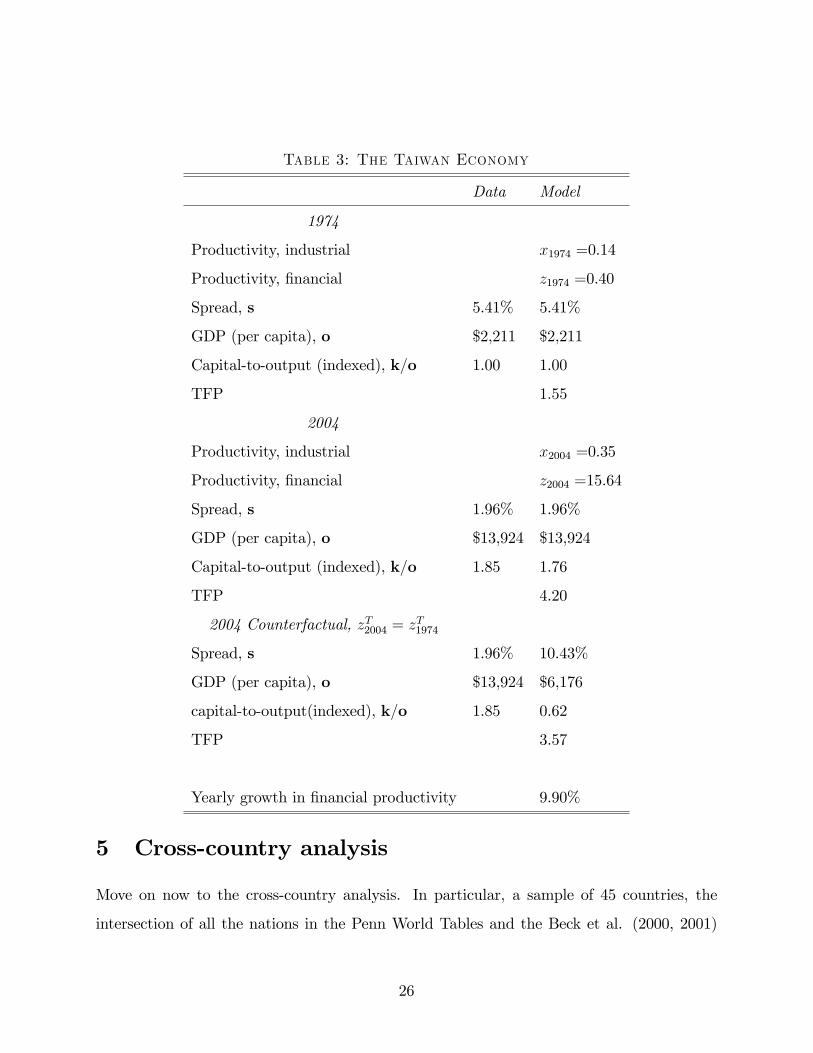
Table 3: The Taiwan Economy
Data Model
1974
Productivity, industrial x1974 =0.14
Productivity, �nancial z1974 =0.40
Spread, s 5.41% 5.41%
GDP (per capita), o $2,211 $2,211
Capital-to-output (indexed), k=o 1.00 1.00
TFP 1.55
2004
Productivity, industrial x2004 =0.35
Productivity, �nancial z2004 =15.64
Spread, s 1.96% 1.96%
GDP (per capita), o $13,924 $13,924
Capital-to-output (indexed), k=o 1.85 1.76
TFP 4.20
2004 Counterfactual, zT2004 = zT1974
Spread, s 1.96% 10.43%
GDP (per capita), o $13,924 $6,176
capital-to-output(indexed), k=o 1.85 0.62
TFP 3.57
Yearly growth in �nancial productivity 9.90%
5 Cross-country analysis
Move on now to the cross-country analysis. In particular, a sample of 45 countries, the
intersection of all the nations in the Penn World Tables and the Beck et al. (2000, 2001)
26

dataset, will be studied. For each country j, a technology vector (xj; zj) is backed out
using data on per-capita GDP and interest-rate spreads (oj; sj), given the procedure implied
by equation (6) while setting p to the estimated parameter vector for the U.S. economy.
Erosa (2001) uses interest-rate spreads to quantify the e¤ects of �nancial intermediation on
occupational choice. It is not a forgone conclusion that this can always be done; that is, that
a set of technology parameters can be found such that (6) always holds.12 (The cross-country
results are reported in Table 10 in the appendix.) By construction the model explains all the
variation in output and interest-rate spreads across countries.13 Still, one could ask how
well the measure for the state of technology in the �nancial sector that is backed out using
the model correlates with independent measures of �nancial intermediation. Here, take the
ratio of private credit by deposit banks and other �nancial institutions to GDP as a measure
of �nancial intermediation as reported by Beck et al. (2000, 2001). (Other measures produce
similar results but reduce the sample size too much.) Additionally, one could examine how
well the model explains cross-country di¤erences in capital-to-GDP ratios.
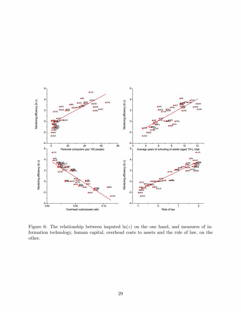
Table 4 reports the �ndings. The correlation between the imputed state of technology
in the �nancial sector and the independent Beck et al. (2000, 2001) measure of �nancial
intermediation is quite high (see Table 4 and Figure 6). Thus, it appears reasonable to
12 Theoretically speaking, there is a maximum interest-rate spread that the model can match. When the�nancial sector becomes too ine¢ cient, it no longer pays to monitor loans. When z falls (relative to x) theaggregate volume of lending declines. The wage rate will decline along with the economy�s capital stock. Asthis happens, the r1�s rise [see (1)]. Take the �rms with the highest value of r1 and denote this by r1. Byde�nition, r1 = r1(�), where � = argmax�2T fr1(�)g. Eventually, r1 will hit er. At this point, a Williamson(1986)-style credit-rationing equilibrium emerges. In the credit-rationing equilibrium, r1 = er. Here type-��rms will pay the �xed interest rate r1 and they will not be monitored. Because r2 > er for these �rms, theywould demand as big a loan as possible. Thus, their credit must be rationed. The interest-rate spread onthese loans will be zero. Note that r1 can never exceed er, because in�nite pro�t opportunities would thenemerge in the economy. Thus, the interest-rate spread is a \-shaped function of z. (The interest-rate spreadalso approaches zero as z !1, or when the economy asymptotes to the frictionless competitive equilibrium.As z ! 0 the fraction of loans that are not monitored eventually approaches 1, implying that the interest-rate spread will drop to zero.) The peak of the \ function is the maximum permissible interest-rate spreadallowed by the model.
13 The model predicts a positive association between a country�s rate of investment and its GDP; Castroet al. (2009, Figure 1) show that this is true. As mentioned, it is stronger when investment spending ismeasured at international prices as opposed to domestic ones. This puzzle could be resolved here by adoptingaspects of Castro et al.�s (2009) two-sector analysis.
27

use the constructed values of z to investigate the relationship between output and �nancial
development. Now the backed-out measure for the e¢ ciency of the �nancial sector correlates
well with a country�s adoption of information technologies (see the upper-left panel in Figure
6). It also is strongly associated with a country�s human capital (upper-right panel) and the
maturity of its legal system (lower-right panel). These three factors should make intermedi-
ation more e¢ cient for the reasons discussed in Section 3. Indeed, Figure 6 (lower-left panel)
also illustrates how the ratio of overhead cost to assets, a measure of e¢ ciency, declines with
the constructed ln(z). Another measure of �nancial e¢ ciency for the model is k=lm; this
was discussed earlier. This too correlates well with the independent Beck et al. (2000, 2001)
measure of �nancial intermediation.
As can be seen, the capital-to-output ratios predicted by the model are positively associ-
ated with those in the data. The correlation is reasonably large. That these two correlations
are not perfect should be expected. Other factors, such as the big di¤erences in public poli-
cies discussed in Parente and Prescott (2000), may explain a large part of the cross-country
di¤erences in capital-to-output ratios. Di¤erences in monetary policies across nations may
in�uence cross-country interest-rate spreads. Additionally, there is noise in these numbers
given the manner of their construction (see the appendix).
Table 4: Cross-Country Evidence
k=o z with Beck et al. (2000, 2001) k=lm with Beck et al. (2000, 2001)
Corr(model, data) 0.62 0.80 0.82
Interestingly, Sri Lanka and the United States both have an interest-rate spread of about
4.2 percent. The model predicts the U.S. z is about 215 percent higher (when ln di¤erenced or
continuously compounded) than Sri Lanka�s� the former�s ln(z) is 2.22 compared with 0.07
for the latter (see Table 10 in the appendix). Recall that the units for ln(z) are meaningless
since monitoring is abstract good. If one measures productivity in the �nancial sector by the
amount of credit extended relative to the amount of labor employed in the �nancial sector,
as discussed earlier, then the analysis suggests that intermediation in the United States is
28
UGA
KENHND
TURGTMNICBRAPERBOLPHLSLVCOLPANMEXLKAIND CRIURY
ZAF
THA DNKESPMUS ITA USAISR FRA SWEPRT GBRAUTBEL NORNLDJPN CHEFIN
AUSIRL
LUX
UGA
KENHND
TURGTM NICBRA PERBOL PHLSLVCOL PANMEXLKAIND CRI URY
ZAF
THA DNKESPMUS ITA USAISRFRA SWEPRT GBRAUT BEL NORNLDJPN CHEFIN
AUSIRL
UGA
KENHNDTURGTMNIC BRAPERBOLPHL SLV
COLPAN MEXLKAIND CRIURYZAF
THA DNKESPMUS ITAUSAISR FRASWEPRT GBRAUTBELNOR NLDJPNCHEFIN
AUSIRL
LUX
UGA
KENHND
TURGTMNIC BRAPER BOLPHLSLVCOL PANMEX LKA IND CRIURY
ZAF
THA DNKESPMUSITA USAISR FRA SWEPRT GBRAUTBEL NORNLDJPN CHEFIN
AUSIRL
LUX
0 20 40 60 804
2
0
2
4
6
Personal computers (per 100 people)
Mon
itorin
g ef
ficien
cy (l
n z)
2 4 6 8 10 124
2
0
2
4
6
Average years of schooling of adults (aged 15+), total
Mon
itorin
g ef
ficien
cy (l
n z)
0.00 0.05 0.104
2
0
2
4
6
Overhead costs/assets ratio
Mon
itorin
g ef
ficien
cy (l
n z)
1 0 1 24
2
0
2
4
6
Rule of law
Mon
itorin
g ef
ficien
cy (l
n z)
Figure 6: The relationship between imputed ln(z) on the one hand, and measures of in-formation technology, human capital, overhead costs to assets and the rule of law, on theother.
29
about 220 percent (continuously compounded) more e¢ cient than in Sri Lanka. Why? The
United States has a much higher level of income per worker and hence TFP than does Sri
Lanka ($33,524 versus $3,967). Therefore, given the higher wages, monitoring will be more
expensive in the United States. For both countries to have the same interest-rate spread,
e¢ ciency in the U.S. �nancial sector must be higher. Before proceeding on to a discussion
of the importance of �nancial development for economic development, note that the �ndings
do not change much if the model is matched up with capital-to-output ratios or overhead
costs (see Figure 6) instead of the Beck et al. (2000, 2001) interest-rate spreads. This is
discussed in Section 6.
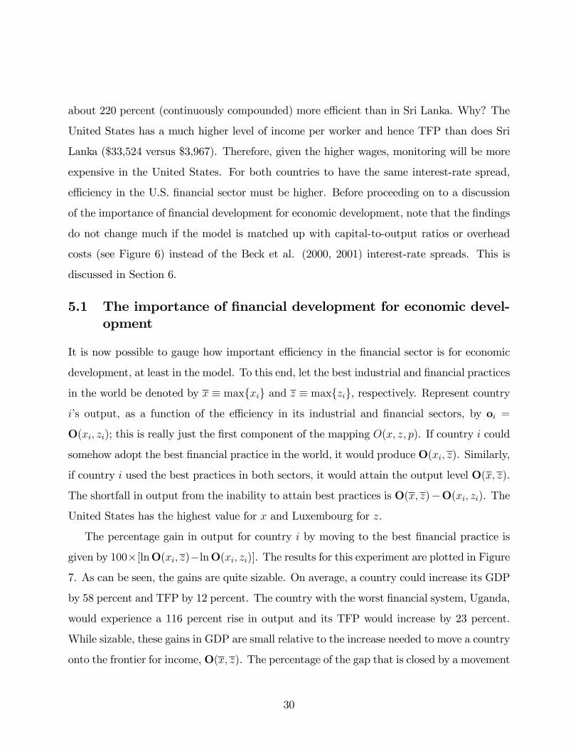
5.1 The importance of �nancial development for economic devel-opment
It is now possible to gauge how important e¢ ciency in the �nancial sector is for economic
development, at least in the model. To this end, let the best industrial and �nancial practices
in the world be denoted by x � maxfxig and z � maxfzig, respectively. Represent country
i�s output, as a function of the e¢ ciency in its industrial and �nancial sectors, by oi =
O(xi; zi); this is really just the �rst component of the mapping O(x; z; p). If country i could
somehow adopt the best �nancial practice in the world, it would produce O(xi; z). Similarly,
if country i used the best practices in both sectors, it would attain the output level O(x; z).
The shortfall in output from the inability to attain best practices is O(x; z)�O(xi; zi). The
United States has the highest value for x and Luxembourg for z.
The percentage gain in output for country i by moving to the best �nancial practice is
given by 100�[lnO(xi; z)�lnO(xi; zi)]. The results for this experiment are plotted in Figure
7. As can be seen, the gains are quite sizable. On average, a country could increase its GDP
by 58 percent and TFP by 12 percent. The country with the worst �nancial system, Uganda,
would experience a 116 percent rise in output and its TFP would increase by 23 percent.
While sizable, these gains in GDP are small relative to the increase needed to move a country
onto the frontier for income, O(x; z). The percentage of the gap that is closed by a movement
30

to best �nancial practice is measured by 100 � [O(xi; z) � O(xi; zi)]=[O(x; z) � O(xi; zi)].
Figure 7 plots the reduction in this gap for the countries in the sample. The average reduction
in this gap is only 33 percent. For most countries the shortfall in output is accounted for by a
low level of TFP in the non�nancial sector. A more detailed breakdown of the cross-country
results is presented in Table 10 in the appendix.
Therefore, the importance of �nancial intermediation for economic development depends
on one�s outlook. World output would rise by 53 percent by moving all countries to the
best �nancial practice (see Table 5). This is a sizable gain. Still, it would close only 31
percent of the gap between actual and potential world output. Dispersion in cross-country
output would fall by about 15 percentage points from 77 percent to 62 percent. Financial
development explains about 23 percent of cross-country dispersion in output by this metric.
Table 5: Worldwide Move to Best Financial Practice, z
Increase in world output (per worker), % 53.3
Reduction in gap between actual and potential world output, % 30.8
Increase in world TFP, % 13.5
Fall in dispersion of ln(output) across countries,% 22.8
Fall in (pop-wghtd) mean of (cap-wghtd) distortion,% 14.7
Fall in (pop-wghtd) mean dispersion of (cap-wghtd) distortion, % 9.5
Restuccia and Rogerson (2008) started a strand in the literature about the importance of
idiosyncratic distortions that create heterogeneity in the prices faced by individual producers.
Although they do not identify the sources of those distortions, they do show they can generate
di¤erences in TFP in the range of 30 to 50 percent. Guner et al. (2008) analyze the possible
impact of size-dependent policies, such as the restrictions on retailing in Japan favoring small
stores, on an economy. Here, the presence of informational frictions causes the expected
marginal product of capital, �1r1 + �2r2, to deviate from its user cost, er. The distortion ismodeled endogenously. De�ne the induced distortion in investment by d = �1r1 + �2r2 � er.For a country such as Uganda these deviations are fairly large. Figure 8 plots the distribution
of the distortion across plants for Luxembourg and Uganda. As can be seen, both the mean
31

020406080
100120
GDP per worker, % change
0
20
40
60
80
100Reduction in the gap to the frontier, %
Turk
eyBr
azil
Ugan
daNi
geria
Guat
emala
Hond
uras
Keny
aNi
cara
gua
Peru
El S
alvad
orUr
ugua
yM
exico
Colom
biaPh
ilippin
esCo
sta R
icaBo
livia
Mor
occo
Sout
h Af
rica
Sri L
anka
Ethio
piaPa
nam
aIn
dia
Denm
ark
Unite
d St
ates
Spai
nIta
lyM
aurit
iusIce
land
Fran
ceIsr
ael
Thail
and
Swed
enUn
ited
King
dom
Portu
gal
Aust
riaNo
rway
Belgi
umNe
ther
lands
Japa
nSw
itzer
land
New
Zeala
ndFi
nland
Aust
ralia
Irelan
dLu
xem
bour
g
0
5
10
15
20
25TFP, % change
Figure 7: Cross-country results showing the impact of a move to �nancial best practice onGDP per worker, the output gap, and TFP�the model.
32

0.0 0.2 0.4 0.6 0.8
0
5
10
15
20
25
Distortion, d
Dens
ityLuxembourg
Uganda
Figure 8: The distribution of distortions, d = �1r1 + �2r2 � er, across establishments forLuxembourg and Uganda�the model.
level of the distortion and its dispersion are much larger in Uganda than in Luxembourg.
The (capital-weighted) mean level of this distortion is 21 percent (2 percent) for Uganda
(Luxembourg). It varies greatly across plants, as indicated by a standard deviation of 18
percent (1.2 percent). If Uganda adopted Luxembourgian �nancial practice, the average size
of this distortion would drop to 0.4 percent. Its standard deviation across plants collapses
from 18 percent to just 0.3 percent. The elimination of this distortion results in capital
deepening among the active plants. Average TFP would rise by 23 percent in the model as
ine¢ cient plants are culled. For the world at large, the average size of the distortion is 16.4
percent with an average coe¢ cient of variation of 62 percent. The mean distortion drops
to 1.7 percent with a worldwide movement to best �nancial practice. The average standard
deviation across plants falls from 10.3 percent to a mere 0.8 percent.
Finally, the model predicts that larger �rms should be found in countries with more
developed �nancial systems. There does not appear to be a dataset that measures �rm size
in a consistent manner across countries. Beck et al. (2006) argue that the best available
33

strategy is to use the size of the largest 100 companies in a country. They �nd a positive
relationship exists between the development of a country�s �nancial system and �rm size,
after controlling for the size of the economy, income per capita, and several �rm and industry
characteristics. As an example, their estimation implies that if Turkey had the same level
of development in the �nancial sector as Korea (a country with a more developed �nancial
system), the average size of the largest �rms in Turkey would more than double.
On this point, imagine running a regression of the following form for both the data and
the model:
ln(size) = constant + � � spread + �� controls:
Firm size in the data is measured by average annual sales per �rm (in U.S. dollars) for the
top 100 �rms, as taken from Beck et al. (2006). For the analogue in the model, simply use
a country�s GDP divided by the measure of active set A to obtain output per �rm. [Once
again the data for interest-rate spreads are obtained from Beck et al. (2000, 2001).] Controls
are added for a country�s GDP and population in the regression for the data, while for the
model they are added just for GDP.14 The same list of countries is used for both the data
and model.
The upshot of the analysis is shown in Table 6. A negative relationship is found in the
cross-country data between the interest-rate spread and average �rm size. The model also
produces a negative relationship between these variables. The similarity between the size
of the interest-rate spread coe¢ cient, �, for the data and model is reassuring. Additionally,
the data estimate of � = �22 implies that if a country with an interest-rate spread of
10 percentage points (which is among the worst 5 percent of nations in terms of �nancial
development) could reduce its spread to just 3 percentage points (which would place it in
the upper 5 percent of countries), then the average size of its top 100 �rms would increase
14 The idea here is that larger countries, as measured by income or population, would tend to have larger�rms. In a frictionless world �rms could locate anywhere, so there would be no need for such a connection tohold. Nontraded goods, productivity di¤erences across countries, restrictions on trade, transportation costs,and so on would all lead to a positive association between average �rm size, on the one hand, and incomeor population, on the other.
34

by 154 percent. This is roughly in accord with Beck et al.�s (2006) �nding discussed above,
given that Turkey had one of the worst �nancial systems while Korea had one of the best.
Table 6: Cross-Country Firm-Size Regressions
Data Model
Interest-rate spread coe¢ cient, � -22.4 -16.6
Standard error for � 2.35 6.55
Number of country observations 27 27
R2 0.80 0.53
6 Robustness analysis: Two alternative matching strate-gies
Two alternative strategies for matching the model with international data will now be in-
vestigated. The story developed here has abstracted away from the importance of �rm-level
�nancing constraints studied by others. The importance of internal �nance in the developed
framework may not be as simple as it may �rst appear. While it may be tempting to draw
on the familiar intuition developed elsewhere on the importance of internal �nance�say in
the debt default literature�it is questionable whether this carries over to the current setting.
The central idea presented here is that unless the owners of a �rm operate it themselves,
they will always have to monitor cash �ows. Otherwise, they run the risk that these �ows
will be expropriated by managers and workers. For example, imagine a publicly listed �rm
that raises all of the funds for its current investment from its cash �ow. Does this mean that
the �rm�s owners (the stockholders) do not need to monitor the company�s cash �ows�of
course not. The point is that they own the sources of all revenue �ows, including those used
for internal �nance, and need a mechanism to verify them. The assumption here is that
the cost of monitoring capital raised from banks and other intermediaries (as measured by
interest-rate spreads) is a good proxy for the cost of monitoring capital more generally, raised
either externally or internally. Suppose, to the contrary, that internal funds do not need to
35

be monitored. Then the importance of the mechanism outlined here would be exaggerated.
Is there evidence of this in the analysis?
If internal funds do not require monitoring, then the model should overstate the impact
of interest-rate spreads on capital-to-output ratios. If so, the model would then display
a steeper relationship between capital-to-output ratios and interest-rate spreads than is
observed in the data. There does not seem to be any evidence of this (see the right-panel of
Figure 9). Indeed, the model does quite well mimicking the relationship between capital-to-
output ratios and interest-rate spreads. Suppose the model is matched up with the observed
capital-to-output ratios, k=o, instead of the observed interest-rate spreads, s. If internal
�nance can be used to reduce the monitoring costs associated with external �nance, then
the backed-out values for the z�s (the productivities of the monitoring technologies) should
now be higher than under the baseline matching scheme for countries with high interest-rate
spreads. In e¤ect, the computed z�s will re�ect a mixture of low-cost internal �nance and
the high-cost external option. The estimated gains from moving to best �nancial practice
should be much smaller. Table 7 reports the results. As can be seen, a worldwide move to
best �nancial practice still leads to a sizable gain in world output and TFP and a large drop
in the dispersion of output across countries. (A listing of the �ndings for each country is
presented in Table 11 in the appendix.)
Table 7: Worldwide Move to Best Financial Practice, z
Matching Methodology
s k=o �
Increase in world output (per worker), % 53.25 48.26 52.12
Reduction in gap between actual and potential world output, % 30.80 25.60 37.01
Increase in world TFP, % 13.47 14.28 13.10
Fall in dispersion of ln(output) across countries,% 22.83 32.82 13.82
Note that in a standard �rm-dynamics model the steady-state capital-to-output ratio
is barely a¤ected by the presence of �nancing constraints. Productive �rms can quickly
accumulate their desired capital stocks in such a setting. Reversing this would require high
36

0.00 0.05 0.10 0.150.00
0.05
0.10
0.15
Interestrate spread
Ove
rhea
d co
sts
0.00 0.05 0.10 0.150
1
2
3
4
k/o, modelk/o, data
Interestrate spread
Capi
talt
oG
DP ra
tio, d
ata
and
mod
el
Figure 9: The right panel shows the relationship between interest-rate spreads and capital-to-output ratios for the data and model. The left panel plots the relationship betweeninterest-rate spreads and overhead costs for the data.
37
death rates for �rms or technology shocks that lack persistence. Indeed, a �rm-dynamics
model with �nancial constraints may have di¢ culty accounting for the observed pattern
of capital-output ratios and interest-rate spreads (Figure 9). Such models often emphasize
a di¤erent mechanism: the impact that �nancing constraints have on TFP, through the
selection of entrepreneurs, as opposed to the impact on the aggregate capital-to-output
ratio.
One could also argue that the �nancial sector is not competitive in less-developed coun-
tries and that this accounts for their high interest-rate spreads. Suppose that the �nancial
sector is monopolized in some countries. Intuitively, one may expect that monopolies might
charge borrowers higher interest rates on loans and o¤er depositors lower rates on their sav-
ings (relative to the situation of perfect competition). Therefore, such monopolistic practices
would be re�ected in interest-rate spreads. These monopolies should still try to minimize
the costs of doing business. In other words, unless there are technological di¤erences across
countries, there should be no correlation between overhead costs and interest-rate spreads.
Yet there is a strong one as Figure 9 (left panel) displays. Furthermore, the �ndings are
similar if these overhead costs, �, are used as a proxy for the e¢ ciency of the �nancial sec-
tor instead of interest-rate spreads, s (shown in Table 7). (Table 12 in the appendix gives
the results for each country.) Thus, the model also works for a direct measure of �nancial
e¢ ciency. (Of course, one could make some type of x-e¢ ciency argument, but developing
this would require a quite di¤erent framework.) Overall the results appear to be remarkably
robust to a variety of matching strategies.
7 Conclusions
Again, how important is �nancial development for economic development? To address this
question, a costly state veri�cation model is applied to both U.S. and cross-country data.
The model has two unique features: First, �nancial intermediaries choose how much la-
bor to devote to monitoring their loan activity. The odds of detecting malfeasance are a
function of this choice. They also depend on the technology used in the �nancial sector.
38

Second, each �rm faces a distribution of returns. Furthermore, there is an economy-wide
distribution across �rms over these �rm-speci�c distributions. These two features lead to a
�nancial theory of �rm size. This occurs because there are diminishing returns to scale in
the monitoring activity. The framework is calibrated to �t the U.S. �rm-size distributions
for 1974 and 2004, as well as the observed intermediation spreads on loans.
The analysis suggests that �nancial intermediation is important for economic develop-
ment. In particular, about 29 percent of U.S. growth can be attributed to technological
improvement in �nancial intermediation. Since there was little change in the U.S. interest-
rate spread, it appears that technological progress in the �nancial sector was in balance with
technological advance in the rest of the economy. Roughly 45 percent of Taiwanese growth
could be attributed to �nancial innovation. Given the dramatic decline in the Taiwanese
interest-rate spread, technological progress in the �nancial sector may have outpaced that
elsewhere.
The model�s predictions for the e¢ ciency of �nancial intermediation in a cross-section
of 45 countries match up well with independent measures. It performs reasonably well in
mimicking cross-country capital-output ratios. The average measured distortion in the world
between the expected marginal product of capital and its user cost is 14.7 percentage points.
The average coe¢ cient of variation in the distortion within a country is 62 percent. World
output could increase by 53 percent if all countries adopted the best �nancial practice in
the world. Adopting this leading-edge practice leads to funds being redirected away from
ine¢ cient �rms toward more productive ones. This reallocation e¤ect is re�ected by a rise in
world TFP by 13.5 percent. Still, this accounts only for 31 percent of the gap between actual
and potential world output because the bulk of the di¤erences in cross-country per-capita
GDP are explained by the huge di¤erences in the productivity of the non�nancial sector.
The results are robust to changes in the matching strategy for backing out the cross-country
productivities in the �nancial and non�nancial sectors.
39

8 Acknowledgments
Olga Itenberg, Diego Restuccia, Cezar Santos, and Stephen Williamson are thanked for
helpful comments. The authors also thank Thorsten Beck for supplying the cross-country
�rm-size data used in Table 6. Feng Dong and Constanza Liborio provided exceptional
research assistance and Judith Ahlers did an excellent job editing the manuscript. This
research was supported by the NSF (award no. 0647766). The views expressed in this paper
are those of the authors and do not necessarily re�ect those of the Federal Reserve Bank of
St. Louis or the Federal Reserve System.
9 Data appendix
� Figure 1: For the United States the spread is computed along the lines of Mehra et
al. (2009). Speci�cally, the spread is de�ned to be �Intermediation services associated
with household borrowing and lending�divided by the �Total amount intermediated�
(see de�nitions of these below). The �Intermediation services associated with house-
hold borrowing and lending�is computed as �Financial Monetary interest paid�minus
�Financial Monetary interest received�minus �Financial services furnished without
payment.�These numbers used are from the National Income and Product Accounts
[NIPA, Tables 7.11 (lines 4 and 28) and 2.4.5 (lines 88)]. The �Total amount interme-
diated�is from the U.S. Flow of Funds Accounts (2000, Table B.100.e). This number is
Assets (line 1) minus Tangible Assets (line 2) minus equity of unincorporated business
(line 29 in Table B.100). For Taiwan, the spread is obtained from Lu (2008). The
initial capital-to-GDP ratio in each country is normalized to 1 (to control for di¤erent
de�nitions of the capital stock).
� Figure 2, Figure 3, and Section 5: The cross-country data for the interest-rate spreads
are from the Financial Structure Dataset assembled by Beck et al. (2000, 2001) and
revised in January 2009. It is de�ned as the accounting value of banks�net interest
as a share of their interest-bearing (total earning) assets averaged over 1997 to 2003.
40

The numbers for the �nancial development measure are from the same dataset. They
represent demand, time, and saving deposits in deposit money banks as a share of GDP
and are also averaged over 1997 to 2003. The other numbers derive from the Penn
World Tables (PWT), version 6.2 [see Heston et al. (2002)]. The aggregate capital
stock for a country, k, is computed for the 1955-2003 sample period. The starting
value is calculated using the formula k = i=(g + �), where i is gross real investment
in purchasing power parity terms (rgdpl*pop*ki in the PWT�s notation or real income
per capita � population � investment�s share in total income), g is the growth rate
in investment, and � is the rate of depreciation. The depreciation rate is taken to be
0.06. For the starting value, i and g are the average over the �rst �ve years available
for each country (in general, 1950 to 1954). Thereafter, a time series is constructed
for each country using the standard formula k0 = k(1 � �) + i: Again, the numbers
used correspond to the average over 1997 to 2003. A country�s TFP is computed using
TFP = (o=l)=(k=l)�, where o is GDP, l is aggregate labor, and � is capital�s share of
income. A value of 0.35 is chosen for �. All three letter country codes in the paper
are taken from the International Organization for Standardization, to wit ISPO 3166-1
alpha-3.
� Figure 5 (�rm size): The data are for establishments and are from County Business
Patterns (CBP), which is released annually by the U.S. Census Bureau. Due to a
signi�cant shift in the methodology employed by the Census beginning in 1974, data
are used only for 1974 and 2004. The horizontal axis orders establishments (from the
smallest to highest) by the percentile in which they lie for employment. The vertical
axis shows the cumulative contribution of this size of establishment to employment in
the U.S. economy. Some data are shown below.
41

Table 9: U.S. Establishment-Size Distribution Data, 1974 & 2004
Establishments with number of workers between:
Series 1-4 5-9 10-19 20-49 50-99 100-249 250-499 500-999 1,000 +
Year 1974
Establishments (in 1,000s) 2,411 739 463 309 103 55.9 17.5 7.61 4.39
Employees (in 1,000s) 4,591 5,222 6,582 9,714 7,223 8,615 6,112 5,286 10,153
Establishments 59% 18% 11% 7.5% 2.5% 1.4% 0.5% 0.2% 0.1%
Employees 7.2% 8.2% 10% 15% 11% 14% 9.6% 8.3% 16%
Year 2004
Establishments (in 1,000s) 4,019 1,406 933 637 218 122 31.3 11.5 6.83
Employees (in 1,000s) 6,791 9,311 12,598 19,251 15,037 18,314 10,662 7,815 15,295
Establishments 54% 19% 13% 8.6% 3.0% 1.7% 0.4% 0.2% 0.1%
Employees 5.9% 8.1% 11% 17% 13% 16% 9.3% 6.8% 13%
Source: U.S. Census Bureau County Business Patterns.
� Figure 6 (relationship between ln z and some other variables): Data for the �rule of
law�are from the World Bank�s �Aggregate Governance Indicators, 1996-2008� [see
Kaufmann et al. (2009)]. Data on personal computers are contained in the World
Bank publication Information and Communications for Development 2009: Extending
Reach and Increasing Impact. The numbers for the �nancial development measure and
the ratio of overhead costs to assets are available in the revised version of the Beck
et al. (2000) dataset mentioned above. In general, overhead costs are the indirect
costs necessary to make a product or provide a service. Examples of such costs are
depreciation, heat, light, indirect materials, indirect labor, insurance, and rent. Finally,
average years of education is based on Barro and Lee (2001).
� Table 6 : The cross-country data on the size of the largest 100 companies in a nation
are derived from Beck et al. (2006); see that source for further details. The data were
kindly supplied by Thorsten Beck.
42
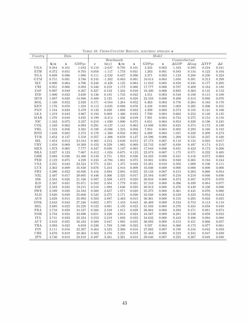
Table 10: Cross-Country Results, matching spreads�s
Country Data ModelBenchmark Counterfactual
k=o s GDPpc x ln(z) k=o s GDPpc s �GDP �Gap �TFP �dUGA 0.284 0.101 1.043 0.110 -2.647 0.795 0.101 3.334 0.002 1.163 0.293 0.234 0.341ETH 0.372 0.031 0.705 0.058 -1.117 1.753 0.031 1.263 0.001 0.583 0.134 0.122 0.104NGA 0.609 0.096 1.086 0.111 -2.532 0.827 0.096 3.371 0.002 1.133 0.288 0.230 0.324GTM 0.751 0.091 3.786 0.245 -1.202 0.863 0.091 10.814 0.004 1.050 0.391 0.213 0.299SLV 0.900 0.064 4.706 0.248 -0.428 1.125 0.064 11.010 0.005 0.850 0.345 0.177 0.205CRI 0.951 0.060 8.093 0.346 0.210 1.172 0.060 17.777 0.006 0.787 0.409 0.164 0.188ZAF 0.997 0.049 8.207 0.327 0.543 1.334 0.049 16.400 0.006 0.692 0.363 0.145 0.153IND 1.006 0.032 2.630 0.136 0.185 1.745 0.032 4.551 0.003 0.548 0.180 0.115 0.100MUS 1.087 0.028 14.986 0.408 2.125 1.851 0.028 22.558 0.006 0.409 0.313 0.086 0.076BOL 1.160 0.052 2.929 0.171 -0.584 1.284 0.052 6.363 0.003 0.776 0.264 0.163 0.170KEN 1.176 0.076 1.258 0.112 -2.035 0.986 0.076 3.428 0.002 1.003 0.265 0.206 0.255PAN 1.184 0.033 2.479 0.133 0.029 1.693 0.033 4.399 0.003 0.574 0.185 0.121 0.106LKA 1.219 0.043 3.967 0.194 0.069 1.466 0.043 7.700 0.004 0.663 0.252 0.140 0.135MAR 1.276 0.049 3.835 0.199 -0.214 1.336 0.049 7.991 0.004 0.734 0.275 0.154 0.158NIC 1.342 0.075 3.337 0.210 -1.030 1.000 0.075 8.651 0.004 0.953 0.339 0.196 0.245COL 1.349 0.062 6.093 0.291 -0.137 1.141 0.062 13.898 0.005 0.825 0.374 0.172 0.199PHL 1.524 0.056 3.565 0.198 -0.506 1.224 0.056 7.954 0.004 0.802 0.293 0.168 0.182HND 1.649 0.082 2.273 0.170 -1.560 0.932 0.082 6.309 0.003 1.021 0.320 0.209 0.273TUR 1.652 0.127 5.559 0.357 -1.306 0.659 0.127 18.596 0.006 1.208 0.525 0.237 0.420IRL 1.854 0.012 24.344 0.465 4.212 2.640 0.012 27.173 0.007 0.110 0.134 0.023 0.017URY 1.858 0.069 10.269 0.423 0.229 1.065 0.069 23.742 0.007 0.838 0.497 0.174 0.215MEX 1.973 0.065 7.777 0.347 0.038 1.107 0.065 17.843 0.006 0.831 0.423 0.173 0.206BRA 2.027 0.123 7.067 0.412 -1.024 0.675 0.123 22.873 0.007 1.175 0.571 0.232 0.405GBR 2.088 0.026 24.400 0.549 2.751 1.924 0.026 34.322 0.008 0.341 0.416 0.072 0.063PER 2.122 0.075 4.220 0.245 -0.794 1.001 0.075 10.801 0.004 0.940 0.365 0.194 0.244USA 2.231 0.042 33.524 0.775 2.221 1.475 0.042 55.381 0.010 0.502 1.000 0.106 0.111LUX 2.362 0.009 45.830 0.676 5.344 2.844 0.009 45.830 0.009 0.000 0.000 0.000 0.000PRT 2.396 0.022 16.936 0.416 2.694 2.085 0.022 23.133 0.007 0.312 0.263 0.066 0.054NZL 2.487 0.017 20.605 0.446 3.366 2.325 0.017 25.584 0.007 0.216 0.219 0.046 0.036ISR 2.504 0.028 21.106 0.507 2.509 1.873 0.028 30.658 0.008 0.373 0.387 0.079 0.070ILD 2.567 0.031 25.071 0.582 2.504 1.779 0.031 37.243 0.008 0.396 0.499 0.084 0.077ESP 2.583 0.035 19.215 0.510 1.988 1.646 0.035 30.913 0.008 0.476 0.449 0.100 0.096SWE 2.599 0.028 24.582 0.560 2.657 1.871 0.028 35.275 0.008 0.361 0.445 0.076 0.068NLD 2.620 0.020 25.600 0.532 3.275 2.171 0.020 32.838 0.008 0.249 0.323 0.053 0.043AUS 2.628 0.015 25.993 0.503 3.887 2.463 0.015 30.361 0.008 0.155 0.205 0.033 0.025DNK 2.642 0.043 27.246 0.682 1.971 1.453 0.043 46.469 0.009 0.534 0.753 0.113 0.118BEL 2.695 0.022 24.228 0.522 3.091 2.105 0.022 31.933 0.008 0.276 0.334 0.058 0.049FRA 2.710 0.029 24.537 0.568 2.549 1.815 0.029 36.004 0.008 0.383 0.471 0.081 0.074NOR 2.734 0.024 32.896 0.651 3.220 2.014 0.024 43.567 0.009 0.281 0.539 0.059 0.052ITA 2.741 0.033 22.234 0.553 2.219 1.692 0.033 34.632 0.008 0.443 0.486 0.094 0.088AUT 2.842 0.025 26.433 0.569 2.947 1.985 0.025 36.093 0.008 0.312 0.421 0.066 0.057THA 3.093 0.022 6.659 0.226 1.789 2.100 0.022 9.597 0.004 0.366 0.173 0.077 0.061FIN 3.111 0.016 22.207 0.464 3.525 2.366 0.016 27.062 0.007 0.198 0.216 0.042 0.033CHE 3.670 0.019 28.363 0.562 3.476 2.221 0.019 35.463 0.008 0.223 0.334 0.047 0.039JPN 3.740 0.018 23.818 0.497 3.381 2.261 0.018 29.840 0.007 0.225 0.267 0.048 0.038
43
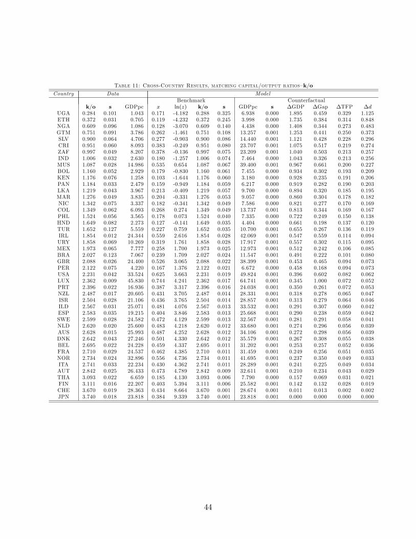
Table 11: Cross-Country Results, matching capital/output ratios�k=o
Country Data ModelBenchmark Counterfactual
k=o s GDPpc x ln(z) k=o s GDPpc s �GDP �Gap �TFP �dUGA 0.284 0.101 1.043 0.171 -4.182 0.288 0.325 6.938 0.000 1.895 0.459 0.329 1.125ETH 0.372 0.031 0.705 0.119 -4.232 0.372 0.245 3.998 0.000 1.735 0.384 0.314 0.848NGA 0.609 0.096 1.086 0.128 -3.070 0.609 0.140 4.438 0.000 1.408 0.344 0.273 0.483GTM 0.751 0.091 3.786 0.262 -1.461 0.751 0.108 13.257 0.001 1.253 0.441 0.250 0.373SLV 0.900 0.064 4.706 0.277 -0.903 0.900 0.086 14.440 0.001 1.121 0.428 0.228 0.296CRI 0.951 0.060 8.093 0.383 -0.249 0.951 0.080 23.707 0.001 1.075 0.517 0.219 0.274ZAF 0.997 0.049 8.207 0.378 -0.136 0.997 0.075 23.209 0.001 1.040 0.503 0.213 0.257IND 1.006 0.032 2.630 0.180 -1.257 1.006 0.074 7.464 0.000 1.043 0.326 0.213 0.256MUS 1.087 0.028 14.986 0.535 0.654 1.087 0.067 39.400 0.001 0.967 0.661 0.200 0.227BOL 1.160 0.052 2.929 0.179 -0.830 1.160 0.061 7.455 0.000 0.934 0.302 0.193 0.209KEN 1.176 0.076 1.258 0.103 -1.644 1.176 0.060 3.180 0.000 0.928 0.235 0.191 0.206PAN 1.184 0.033 2.479 0.159 -0.949 1.184 0.059 6.217 0.000 0.919 0.282 0.190 0.203LKA 1.219 0.043 3.967 0.213 -0.409 1.219 0.057 9.700 0.000 0.894 0.320 0.185 0.195MAR 1.276 0.049 3.835 0.204 -0.331 1.276 0.053 9.057 0.000 0.860 0.304 0.178 0.182NIC 1.342 0.075 3.337 0.182 -0.341 1.342 0.049 7.586 0.000 0.821 0.277 0.170 0.169COL 1.349 0.062 6.093 0.268 0.274 1.349 0.049 13.737 0.001 0.813 0.344 0.169 0.167PHL 1.524 0.056 3.565 0.178 0.073 1.524 0.040 7.335 0.000 0.722 0.249 0.150 0.138HND 1.649 0.082 2.273 0.127 -0.141 1.649 0.035 4.404 0.000 0.661 0.198 0.137 0.120TUR 1.652 0.127 5.559 0.227 0.759 1.652 0.035 10.700 0.001 0.655 0.267 0.136 0.119IRL 1.854 0.012 24.344 0.559 2.616 1.854 0.028 42.069 0.001 0.547 0.559 0.114 0.094URY 1.858 0.069 10.269 0.319 1.761 1.858 0.028 17.917 0.001 0.557 0.302 0.115 0.095MEX 1.973 0.065 7.777 0.258 1.700 1.973 0.025 12.973 0.001 0.512 0.242 0.106 0.085BRA 2.027 0.123 7.067 0.239 1.709 2.027 0.024 11.547 0.001 0.491 0.222 0.101 0.080GBR 2.088 0.026 24.400 0.526 3.065 2.088 0.022 38.399 0.001 0.453 0.465 0.094 0.073PER 2.122 0.075 4.220 0.167 1.376 2.122 0.021 6.672 0.000 0.458 0.168 0.094 0.073USA 2.231 0.042 33.524 0.625 3.663 2.231 0.019 49.824 0.001 0.396 0.602 0.082 0.062LUX 2.362 0.009 45.830 0.744 4.241 2.362 0.017 64.741 0.001 0.345 1.000 0.072 0.052PRT 2.396 0.022 16.936 0.387 3.317 2.396 0.016 24.038 0.001 0.350 0.261 0.072 0.053NZL 2.487 0.017 20.605 0.431 3.705 2.487 0.014 28.331 0.001 0.318 0.278 0.065 0.047ISR 2.504 0.028 21.106 0.436 3.765 2.504 0.014 28.857 0.001 0.313 0.279 0.064 0.046ILD 2.567 0.031 25.071 0.481 4.076 2.567 0.013 33.532 0.001 0.291 0.307 0.060 0.042ESP 2.583 0.035 19.215 0.404 3.846 2.583 0.013 25.668 0.001 0.290 0.238 0.059 0.042SWE 2.599 0.028 24.582 0.472 4.129 2.599 0.013 32.567 0.001 0.281 0.291 0.058 0.041NLD 2.620 0.020 25.600 0.483 4.218 2.620 0.012 33.680 0.001 0.274 0.296 0.056 0.039AUS 2.628 0.015 25.993 0.487 4.252 2.628 0.012 34.106 0.001 0.272 0.298 0.056 0.039DNK 2.642 0.043 27.246 0.501 4.330 2.642 0.012 35.579 0.001 0.267 0.308 0.055 0.038BEL 2.695 0.022 24.228 0.459 4.337 2.695 0.011 31.202 0.001 0.253 0.257 0.052 0.036FRA 2.710 0.029 24.537 0.462 4.385 2.710 0.011 31.459 0.001 0.249 0.256 0.051 0.035NOR 2.734 0.024 32.896 0.556 4.736 2.734 0.011 41.695 0.001 0.237 0.350 0.049 0.033ITA 2.741 0.033 22.234 0.430 4.362 2.741 0.011 28.289 0.001 0.241 0.225 0.049 0.034AUT 2.842 0.025 26.433 0.473 4.789 2.842 0.009 32.611 0.001 0.210 0.234 0.043 0.029THA 3.093 0.022 6.659 0.185 4.130 3.093 0.006 7.790 0.000 0.157 0.069 0.031 0.021FIN 3.111 0.016 22.207 0.403 5.394 3.111 0.006 25.582 0.001 0.142 0.132 0.028 0.019CHE 3.670 0.019 28.363 0.434 8.664 3.670 0.001 28.674 0.001 0.011 0.013 0.002 0.002JPN 3.740 0.018 23.818 0.384 9.339 3.740 0.001 23.818 0.001 0.000 0.000 0.000 0.000
44

Table 12: Cross-Country Results, matching overhead costs��
Country Data ModelBenchmark Counterfactual
k=o � GDPpc x ln(z) k=o � GDPpc s �GDP �Gap �TFP �dUGA 0.284 0.072 1.043 0.097 -2.136 1.027 0.072 2.707 0.003 0.954 0.250 0.197 0.239ETH 0.372 0.024 0.705 0.053 -0.591 2.030 0.024 1.107 0.002 0.451 0.107 0.095 0.075NGA 0.609 0.076 1.086 0.102 -2.184 0.986 0.076 2.899 0.003 0.982 0.260 0.202 0.253EGY 0.638 0.018 4.481 0.167 1.751 2.281 0.018 5.966 0.005 0.286 0.121 0.060 0.046GTM 0.751 0.072 3.786 0.225 -0.838 1.032 0.072 9.144 0.006 0.882 0.349 0.182 0.228SLV 0.900 0.040 4.706 0.212 0.374 1.536 0.040 8.397 0.006 0.579 0.251 0.122 0.118CRI 0.951 0.055 8.093 0.336 0.350 1.242 0.055 16.167 0.008 0.692 0.391 0.145 0.164ZAF 0.997 0.054 8.207 0.337 0.388 1.255 0.054 16.262 0.008 0.684 0.390 0.143 0.161IND 1.006 0.023 2.630 0.125 0.736 2.036 0.023 3.926 0.004 0.401 0.139 0.084 0.068MUS 1.087 0.027 14.986 0.403 2.207 1.895 0.027 20.913 0.009 0.333 0.289 0.071 0.063BOL 1.160 0.043 2.929 0.160 -0.259 1.453 0.043 5.606 0.005 0.649 0.233 0.137 0.134KEN 1.176 0.054 1.258 0.099 -1.479 1.259 0.054 2.790 0.003 0.797 0.220 0.167 0.176PAK 1.184 0.027 2.479 0.126 0.385 1.883 0.027 3.939 0.004 0.463 0.157 0.098 0.082LKA 1.219 0.040 3.967 0.191 0.165 1.516 0.040 7.226 0.005 0.600 0.242 0.126 0.122MAR 1.276 0.023 3.835 0.159 1.150 2.055 0.023 5.573 0.005 0.374 0.149 0.079 0.064NIC 1.342 0.076 3.337 0.212 -1.057 0.987 0.076 8.383 0.006 0.921 0.347 0.190 0.244COL 1.349 0.085 6.093 0.326 -0.631 0.906 0.085 15.522 0.008 0.935 0.456 0.191 0.269PHL 1.524 0.044 3.565 0.182 -0.072 1.448 0.044 6.765 0.005 0.641 0.248 0.135 0.134HND 1.649 0.048 2.273 0.140 -0.678 1.367 0.048 4.617 0.004 0.709 0.233 0.149 0.151TUR 1.652 0.065 5.559 0.278 -0.291 1.110 0.065 12.398 0.007 0.802 0.374 0.167 0.201PAN 1.807 0.028 7.847 0.266 1.532 1.879 0.028 11.634 0.007 0.394 0.219 0.083 0.073IRL 1.854 0.011 24.344 0.457 4.440 2.736 0.011 24.865 0.010 0.021 0.032 0.005 0.003URY 1.858 0.087 10.269 0.461 -0.142 0.891 0.087 25.210 0.010 0.898 0.587 0.183 0.268ARG 1.934 0.086 10.983 0.479 -0.051 0.902 0.086 26.572 0.010 0.884 0.604 0.180 0.262VEN 1.946 0.082 7.216 0.359 -0.402 0.934 0.082 17.756 0.008 0.900 0.478 0.184 0.256MEX 1.973 0.071 7.777 0.358 -0.114 1.034 0.071 17.730 0.008 0.824 0.456 0.170 0.219BRA 2.027 0.077 7.067 0.346 -0.329 0.977 0.077 16.893 0.008 0.871 0.458 0.179 0.240GBR 2.088 0.036 24.400 0.600 2.179 1.621 0.036 36.183 0.012 0.394 0.593 0.083 0.084PER 2.122 0.062 4.220 0.228 -0.485 1.151 0.062 9.363 0.006 0.797 0.330 0.166 0.193USA 2.231 0.035 33.524 0.733 2.538 1.642 0.035 47.412 0.014 0.347 1.000 0.073 0.075TTO 2.283 0.036 13.600 0.410 1.597 1.622 0.036 21.425 0.009 0.455 0.364 0.096 0.094LUX 2.362 0.013 45.830 0.715 4.644 2.551 0.013 45.830 0.013 0.000 0.000 0.000 0.000PRT 2.396 0.021 16.936 0.410 2.793 2.136 0.021 21.419 0.009 0.235 0.228 0.050 0.042NZL 2.487 0.026 20.605 0.491 2.605 1.936 0.026 27.431 0.010 0.286 0.343 0.061 0.054ISR 2.504 0.025 21.106 0.494 2.687 1.967 0.025 27.716 0.010 0.273 0.337 0.058 0.052ESP 2.583 0.031 19.215 0.494 2.190 1.753 0.031 27.659 0.010 0.364 0.403 0.077 0.073SWE 2.599 0.032 24.582 0.583 2.394 1.731 0.032 34.770 0.012 0.347 0.528 0.073 0.071CAN 2.609 0.037 26.138 0.633 2.204 1.597 0.037 38.844 0.012 0.396 0.665 0.084 0.086NLD 2.620 0.025 25.600 0.562 2.855 1.954 0.025 33.080 0.011 0.256 0.416 0.054 0.049AUS 2.628 0.048 25.993 0.686 1.736 1.355 0.048 43.339 0.013 0.511 0.851 0.107 0.122DNK 2.642 0.040 27.246 0.668 2.090 1.515 0.040 41.804 0.013 0.428 0.773 0.090 0.096BEL 2.695 0.026 24.228 0.546 2.755 1.930 0.026 31.776 0.011 0.271 0.404 0.057 0.052FRA 2.710 0.034 24.537 0.594 2.272 1.667 0.034 35.645 0.012 0.373 0.567 0.079 0.078NOR 2.734 0.028 32.896 0.681 2.910 1.850 0.028 42.907 0.013 0.266 0.727 0.056 0.054ITA 2.741 0.045 22.234 0.606 1.700 1.417 0.045 36.602 0.012 0.499 0.658 0.105 0.115AUT 2.842 0.043 26.433 0.668 1.952 1.459 0.043 41.799 0.013 0.458 0.784 0.097 0.105THA 3.093 0.023 6.659 0.229 1.687 2.047 0.023 9.377 0.006 0.342 0.174 0.072 0.060FIN 3.111 0.016 22.207 0.462 3.576 2.391 0.016 25.219 0.010 0.127 0.168 0.027 0.022CHE 3.670 0.048 28.363 0.724 1.839 1.363 0.048 46.597 0.014 0.497 0.966 0.104 0.119JPN 3.740 0.017 23.818 0.489 3.527 2.333 0.017 27.333 0.010 0.138 0.200 0.029 0.024
References
Barro, R.J., Lee, J.-W., 2001.International data on educational attainment: Updatesand implications. Oxford Economic Papers 53, 541-563.
45

Beck, T., Demirgürç-Kunt, A., Levine, R., 2000. A new database on �nancial develop-ment and structure. World Bank Economic Review 14, 597-605.
Beck, T., Demirgürç-Kunt, A., Levine, R., 2001. The �nancial structure database. In:Demirgürç-Kunt, A., Levine, R. (Eds.), Financial Structure and Economic Growth:A Cross-Country Comparison of Banks Markets, and Development. MIT Press, Cam-bridge, pp. 17-80.
Beck, T., Demirgürç-Kunt, A., Maksimovic, V., 2006. The in�uence of �nanical andlegal institutions on �rm size. Journal of Banking and Finance 30, 2995-3015.
Berger, A.N., 2003. The economic e¤ects of technological progress: Evidence from thebanking industry. Journal of Money, Credit, and Banking 35, 141-176.
Boyd, J.H., Prescott, E.C., 1986. Financial intermediary-coalitions. Journal of Eco-nomic Theory 38, 211-232.
Buera, F.J., Kaboski, J.P., Shin, Y., 2011. Finance and development: A tale of twosectors. American Economic Review 101, 1964�2002.
Caselli, F., Gennaioli, N., Forthcoming. Dynastic management. Economic Inquiry.
Castro, R., Clementi, G. L., MacDonald, G.M., 2009. Legal institutions, sectoral het-erogeneity, and economic development. Review of Economics Studies 76, 529-561.
Cole, H.L., Greenwood, J., Sanchez, J.M., 2012. Why doesn�t technology �ow from richto poor countries? Manuscript. Department of Economics, University of Pennsylvania.
Cooley, T.F., Prescott, E.C., 1995. Economic growth and business cycles. In: Cooley,T.F. (Ed.), Frontiers of Business Cycle Research. Princeton University Press, Prince-ton, pp. 1�38.
Corrado, C.A., Hulten, C.R., Sichel, D.E., 2006. Intangible capital and economicgrowth. Working Paper No. 11948, National Bureau of Economic Research.
Erosa, A., 2001. Financial intermediation and occupational choice in development.Review of Economic Dynamics 4, 303-334.
Erosa, A., Hidalgo Cabrillana, A., 2008. On capital market imperfections as a sourceof low TFP and economic rents. International Economic Review 49, 437-473.
Goldsmith, R.W., 1969. Financial Structure and Development. Yale University Press,New Haven.
Gomme, P., Rupert, R., 2007. �Theory, measurement and calibration of macroeco-nomic models.�Journal of Monetary Economics 54, 460-497.
46
Greenwood, J., Jovanovic, B., 1990. Financial development, growth, and the distribu-tion of income. Journal of Political Economy 98, 1076-1107.
Greenwood, J, Wang, C., Sanchez, J.M., 2010. Financing development: The role ofinformation costs. American Economic Review 100, 1875-1891.
Guner, N., Ventura, G., Xu, D., 2008. Macroeconomic implications of size-dependentpolicies. Review of Economic Dynamics 11, 721-744.
Heston, A., Summers, R., Aten, A., 2002. Penn World Tables, Version 6.1, Center forInternational Comparisons at the University of Pennsylvania (CICUP).
Kaufmann, D., Kraay, A., Mastruzzi, M., 2009. Governance matters VIII: aggregateand individual governance indicators, 1996-2008. Policy Research Working Paper No.4978, The World Bank.
King, R.G., Levine, R., 1993. �Finance and growth: Schumpeter might be right.�Quarterly Journal of Economics 108, 717-736.
King, R.G., Levine, R., 1994. Capital fundamentalism, economic development, andeconomic growth. Carnegie-Rochester Conference Series on Public Policy 40, 259-292.
Levine, R., 2005. Finance and growth: theory and evidence. In: Aghion, P., Durlauf,S.N. (Eds.) Handbook of Economic Growth. Volume 1A. Elsevier B.V., Amsterdam,pp. 865-934.
Li, W., Sarte, P.-D., 2004. Progressive taxation and long-run growth. American Eco-nomic Review 94, 1705�1716.
Lu, S., 2008. The role of capital market e¢ ciency in long-term growth: A quantitativeexploration. Working Paper, Department of Economics, National Tsing Hua University.
Lucas, R.J., Jr., 1978. On the size distribution of business �rms. Bell Journal of Eco-nomics 9, 508-23.
Mehra, R., Piguillem, F., Prescott, E.C., 2009. �Intermediated quantities and returns.�Working Paper No. 14351, National Bureau of Economic Research.
Midrigan, V., Xu, D., 2010. Finance and misallocation: Evidence from plant-level data.Manuscript. Department of Economics, New York University.
Parente, S.L., Prescott, E.C., 2000. Barriers to Riches. The MIT Press, Cambridge,MA.
Restuccia, D., Rogerson, R., 2008. Policy distortions and aggregate productivity withheterogeneous plants. Review of Economic Dynamics 11, 707-720.
47

Siegel, J.J., 1992. The real rate of interest from 1800-1990: A study of the U.S. andthe U.K. Journal of Monetary Economics 29, 227-252.
Townsend, R.M., 1979. Optimal contracts and competitive markets with costly stateveri�cation. Journal of Economic Theory 21, 256-293.
Townsend, R.M., Ueda, K., 2010. Welfare gains from �nancial liberalization. Interna-tional Economic Review 51, 553-597.
Williamson, S.D., 1986. Costly monitoring, �nancial intermediation, and equilibriumcredit rationing. Journal of Monetary Economics 18, 159-79.
48