QUANTIFYING WETLAND TYPE AND ECOSYSTEM SERVICES WITH HYPERSPATIAL UAS IMAGERY

Whitney P. Broussard III

GEOG 596ACapstone Proposal

Fall 2016

Visser 2012

Robert P. Brooks Jenneke M. VisserTom Cousté

• 4,870 sq. km of land lost since the 1930s (area of NJ)

• Potential to lose an additional 4,500 sq. km

• 18% of US oil and 24% of US gas production totaling $16B USD per year• 1st in the nation in total shipping tonnage - 20% of the nation's waterborne commerce• $2.8B USD fisheries industry in Louisiana - 16% of US fisheries come from Louisiana coast

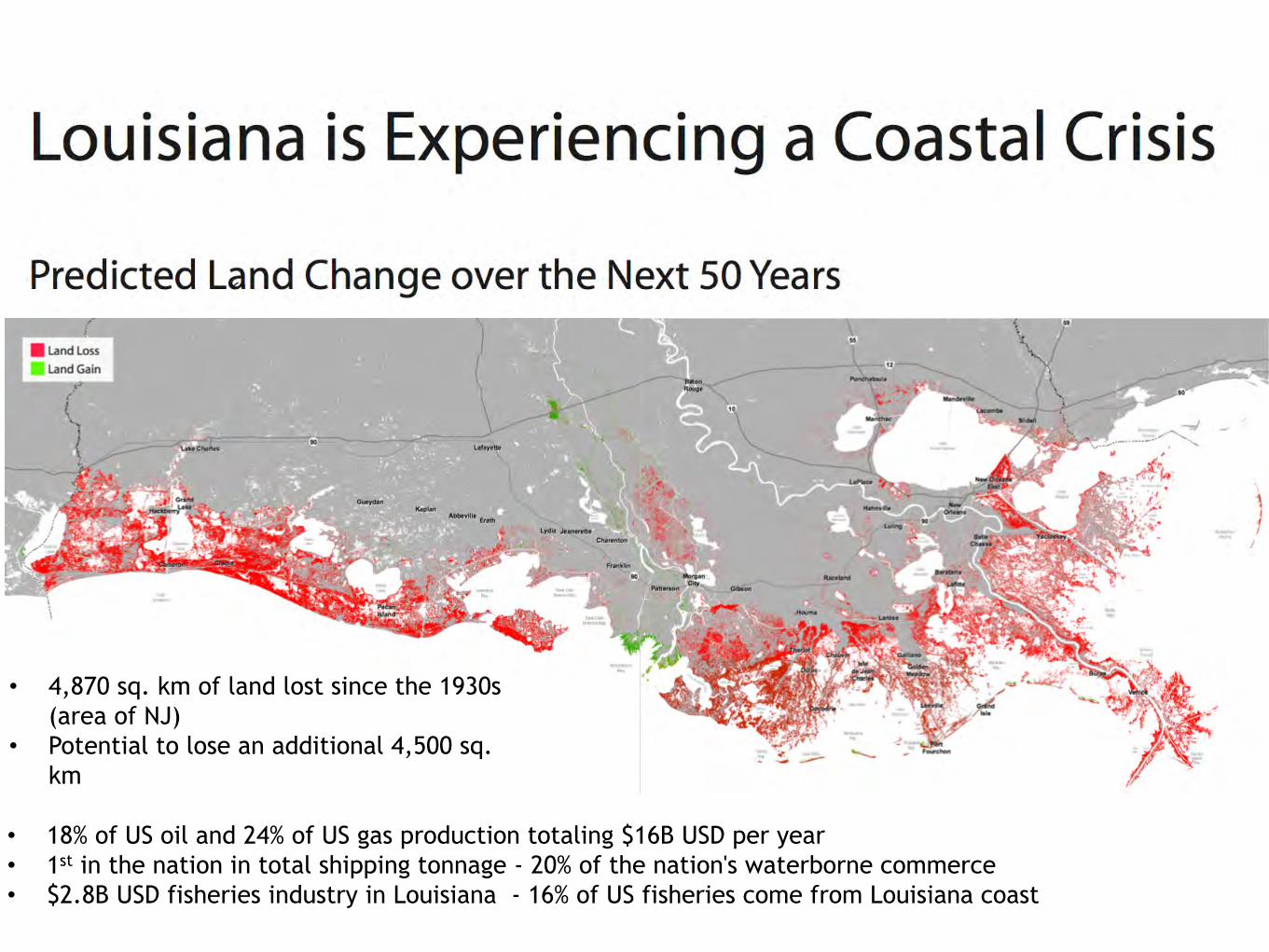
Coastal Louisiana - Master Plan – The Problem and Laboratory

US $50B – 50 year plan

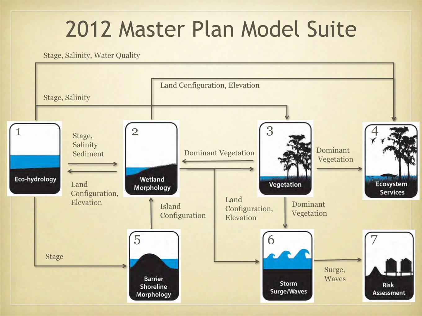
Surge

Upper Trophic

Stage,Salinity Sediment

Stage, Salinity

Stage, Salinity, Water Quality

Dominant Vegetation

DominantVegetation

Land Configuration, Elevation

Land Configuration, Elevation

Stage

Island Configuration

Land Configuration, Elevation

Surge, Waves

Dominant Vegetation

1 3

5 7

2 4

6

2012 Master Plan Model Suite

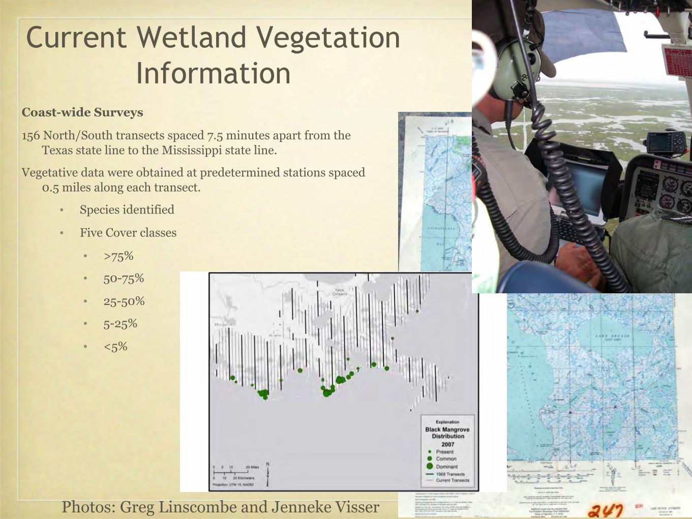
Current Wetland Vegetation Information

Coast-wide Surveys

156 North/South transects spaced 7.5 minutes apart from the Texas state line to the Mississippi state line.

Vegetative data were obtained at predetermined stations spaced 0.5 miles along each transect.

• Species identified

• Five Cover classes

• >75%

• 50-75%

• 25-50%

• 5-25%

• <5%

Photos: Greg Linscombe and Jenneke Visser

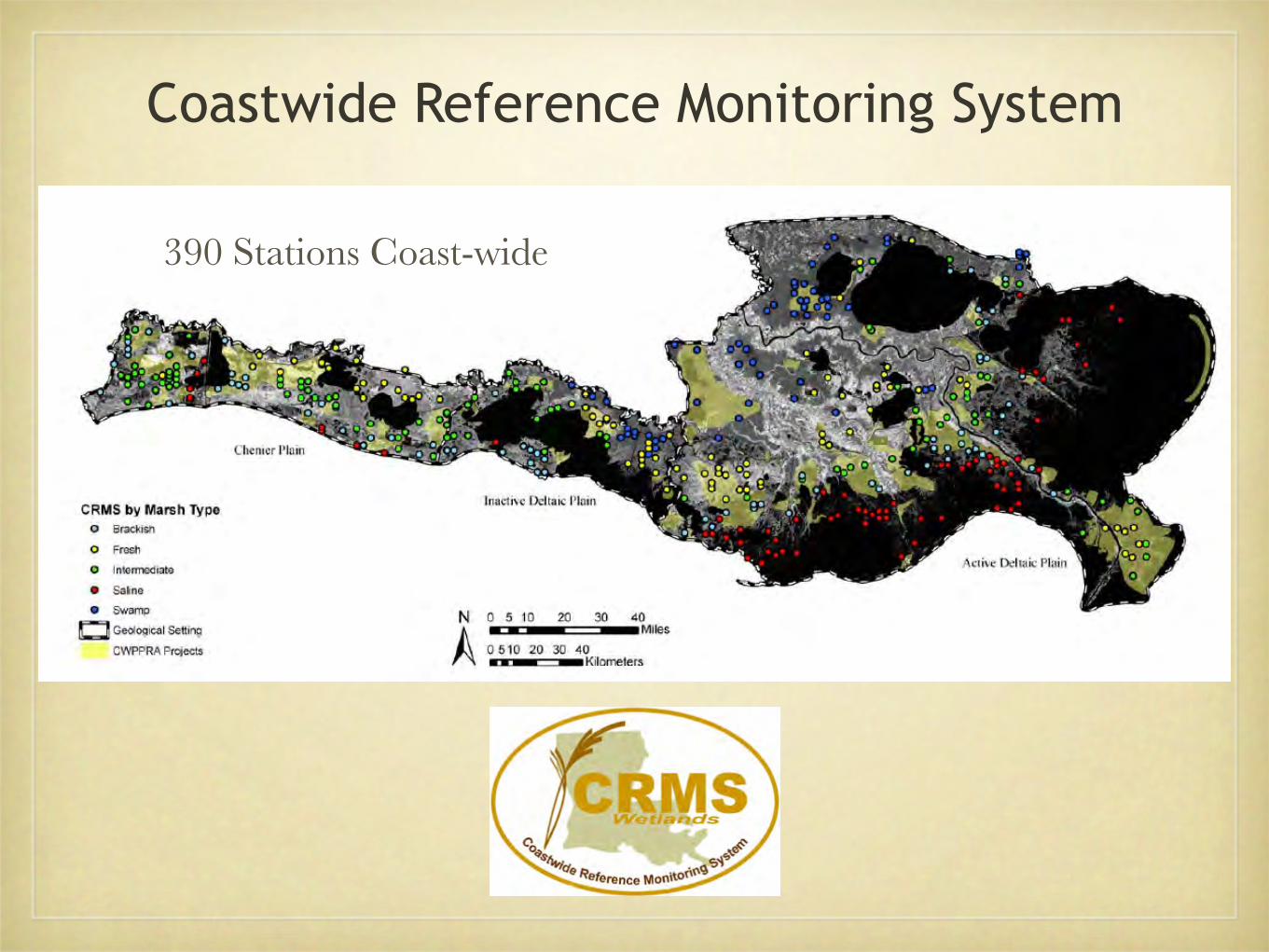
Coastwide Reference Monitoring System

390 Stations Coast-wide

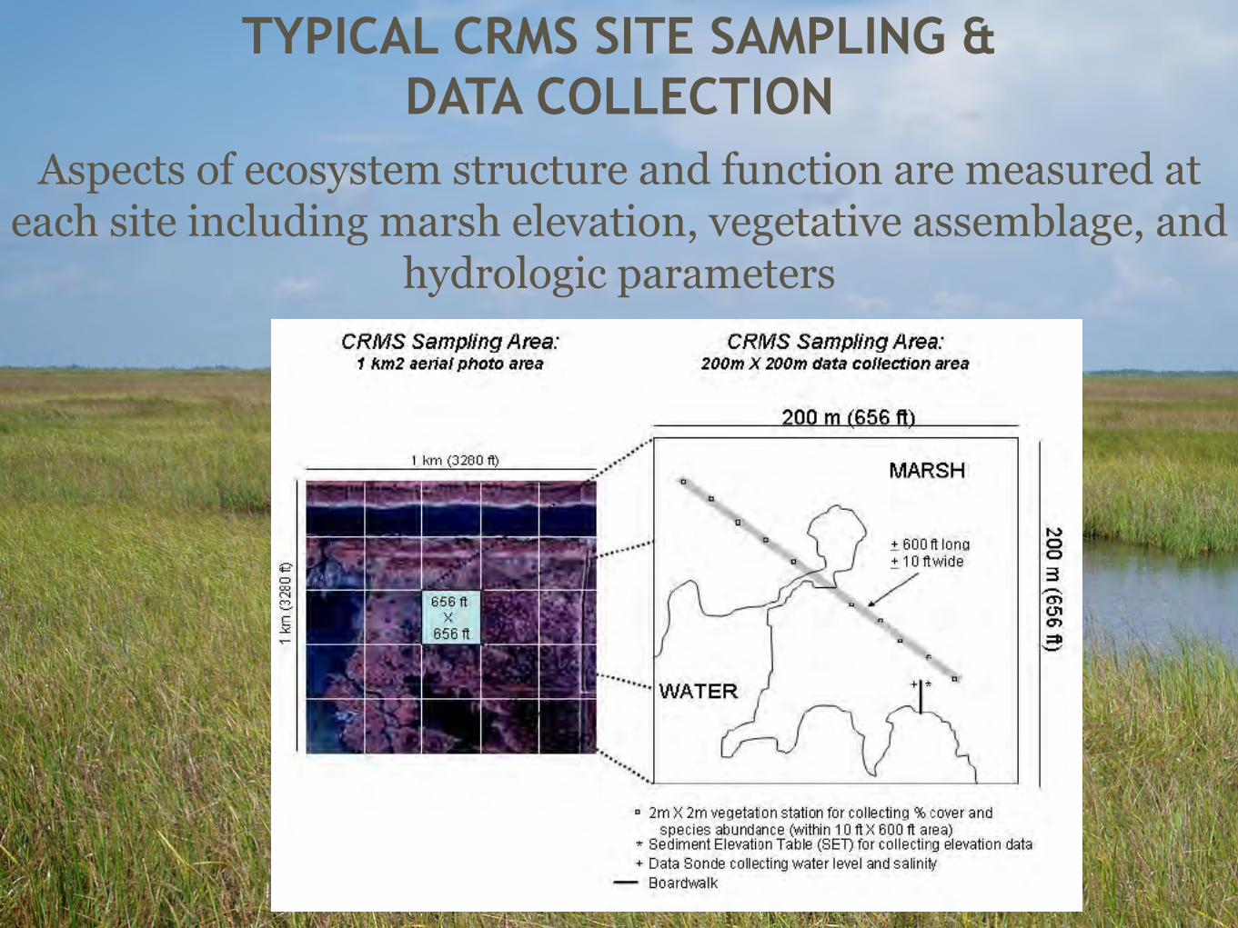
TYPICAL CRMS SITE SAMPLING &DATA COLLECTION

Aspects of ecosystem structure and function are measured at each site including marsh elevation, vegetative assemblage, and

hydrologic parameters

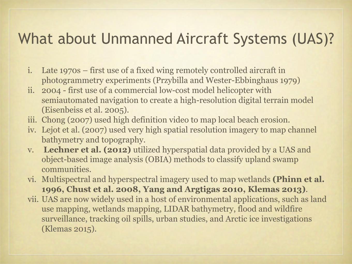
i. Late 1970s – first use of a fixed wing remotely controlled aircraft in photogrammetry experiments (Przybilla and Wester-Ebbinghaus 1979)

ii. 2004 - first use of a commercial low-cost model helicopter with semiautomated navigation to create a high-resolution digital terrain model (Eisenbeiss et al. 2005).

iii. Chong (2007) used high definition video to map local beach erosion.iv. Lejot et al. (2007) used very high spatial resolution imagery to map channel

bathymetry and topography.v. Lechner et al. (2012) utilized hyperspatial data provided by a UAS and

object-based image analysis (OBIA) methods to classify upland swamp communities.

vi. Multispectral and hyperspectral imagery used to map wetlands (Phinn et al. 1996, Chust et al. 2008, Yang and Argtigas 2010, Klemas 2013).

vii. UAS are now widely used in a host of environmental applications, such as land use mapping, wetlands mapping, LIDAR bathymetry, flood and wildfire surveillance, tracking oil spills, urban studies, and Arctic ice investigations (Klemas 2015).

What about Unmanned Aircraft Systems (UAS)?

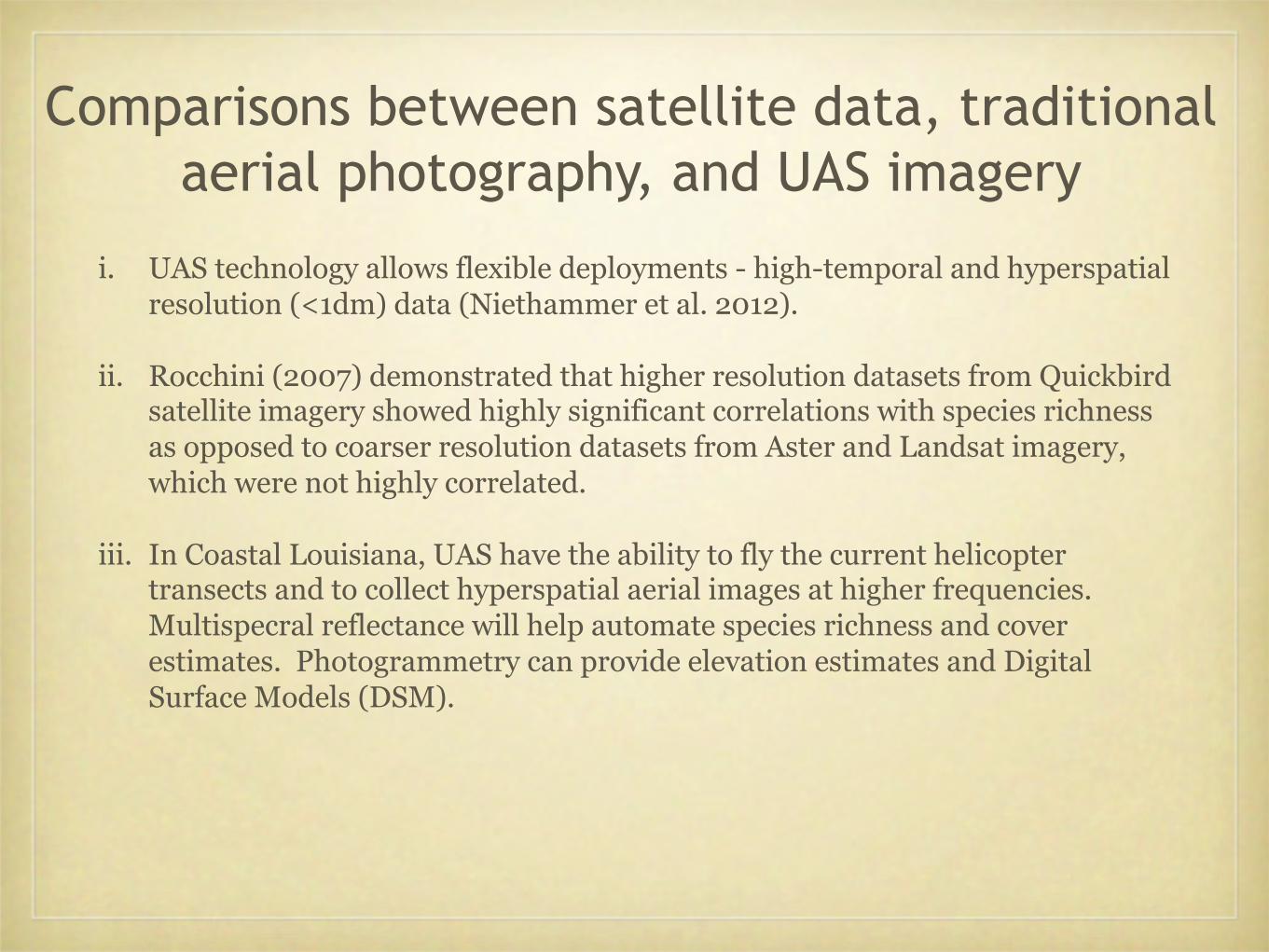
Comparisons between satellite data, traditional aerial photography, and UAS imagery

i. UAS technology allows flexible deployments - high-temporal and hyperspatial resolution (<1dm) data (Niethammer et al. 2012).

ii. Rocchini (2007) demonstrated that higher resolution datasets from Quickbirdsatellite imagery showed highly significant correlations with species richness as opposed to coarser resolution datasets from Aster and Landsat imagery, which were not highly correlated.

iii. In Coastal Louisiana, UAS have the ability to fly the current helicopter transects and to collect hyperspatial aerial images at higher frequencies. Multispecral reflectance will help automate species richness and cover estimates. Photogrammetry can provide elevation estimates and Digital Surface Models (DSM).

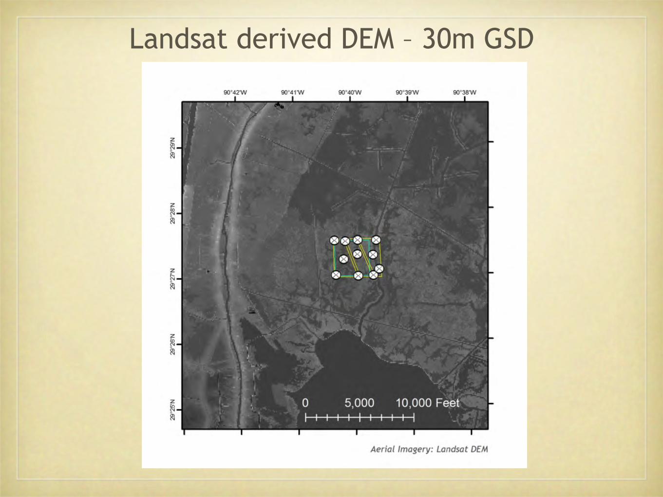
Landsat derived DEM – 30m GSD

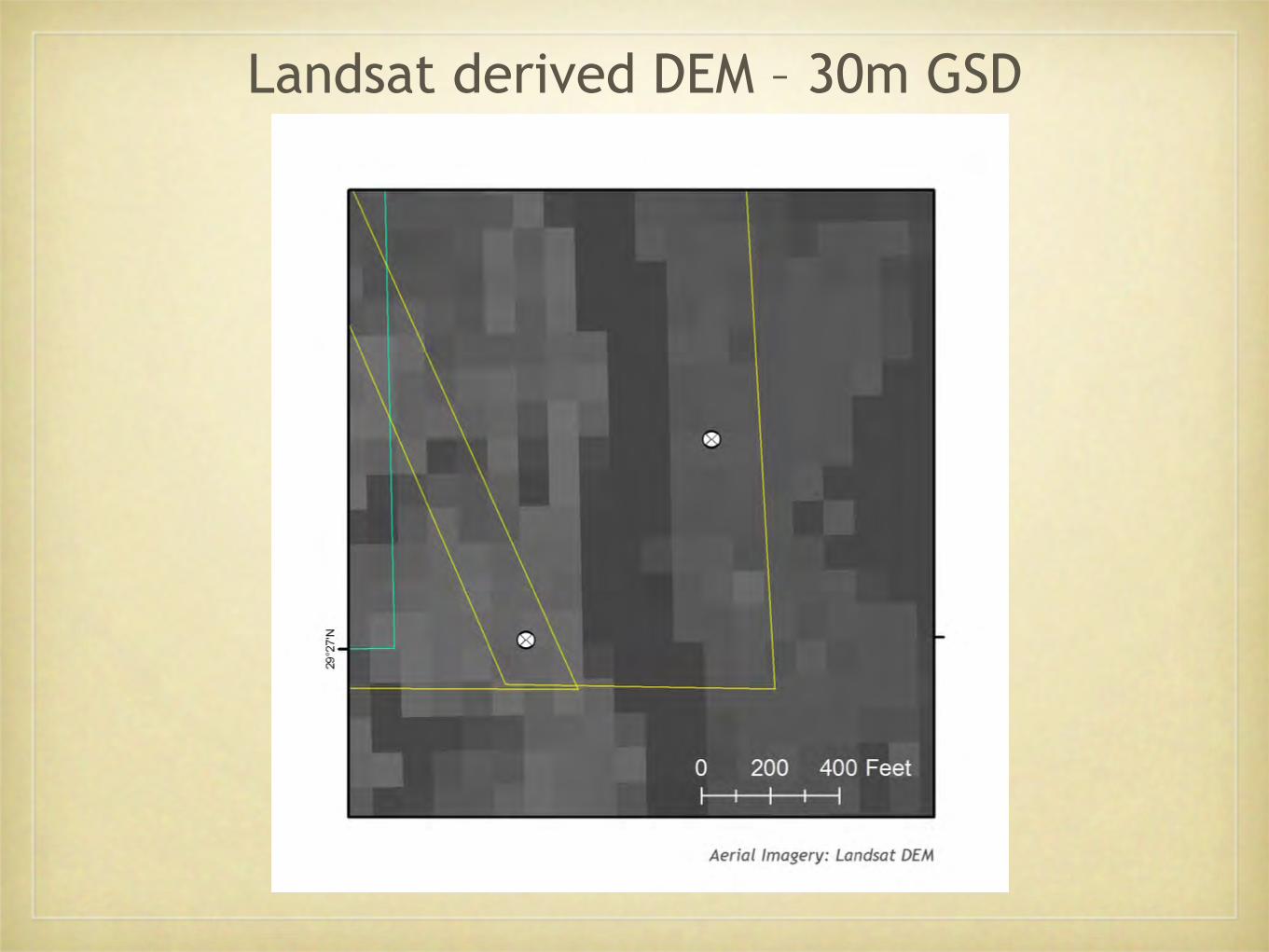
Landsat derived DEM – 30m GSD

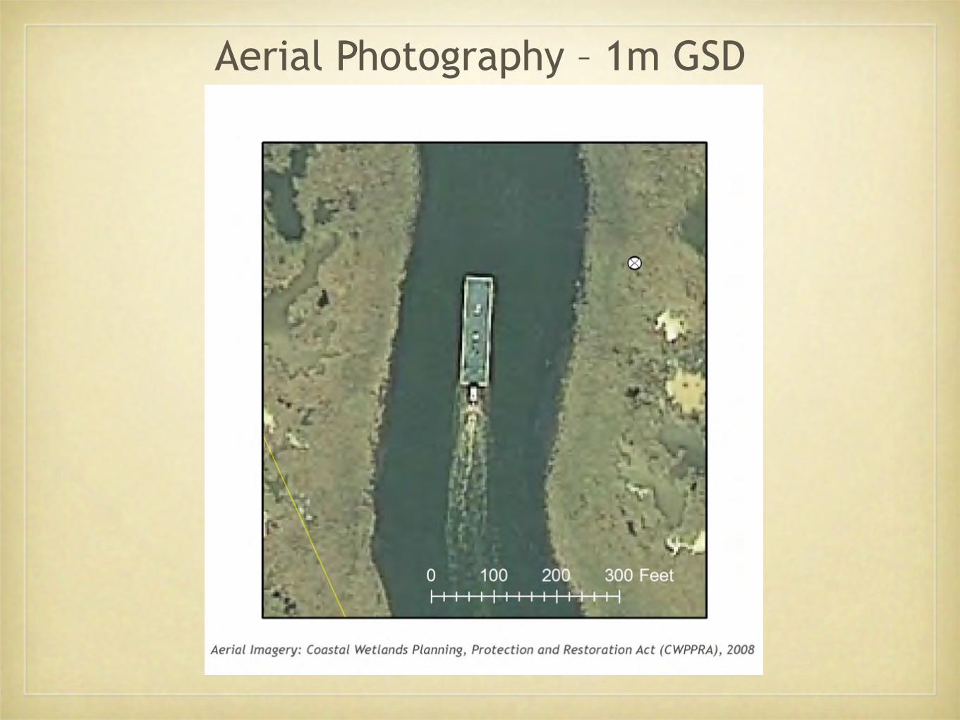
Aerial Photography – 1m GSD

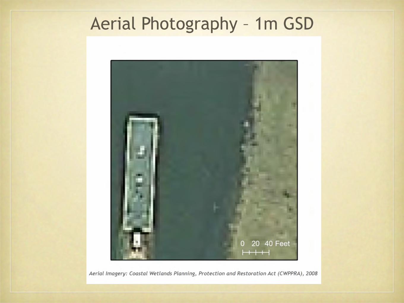
Aerial Photography – 1m GSD

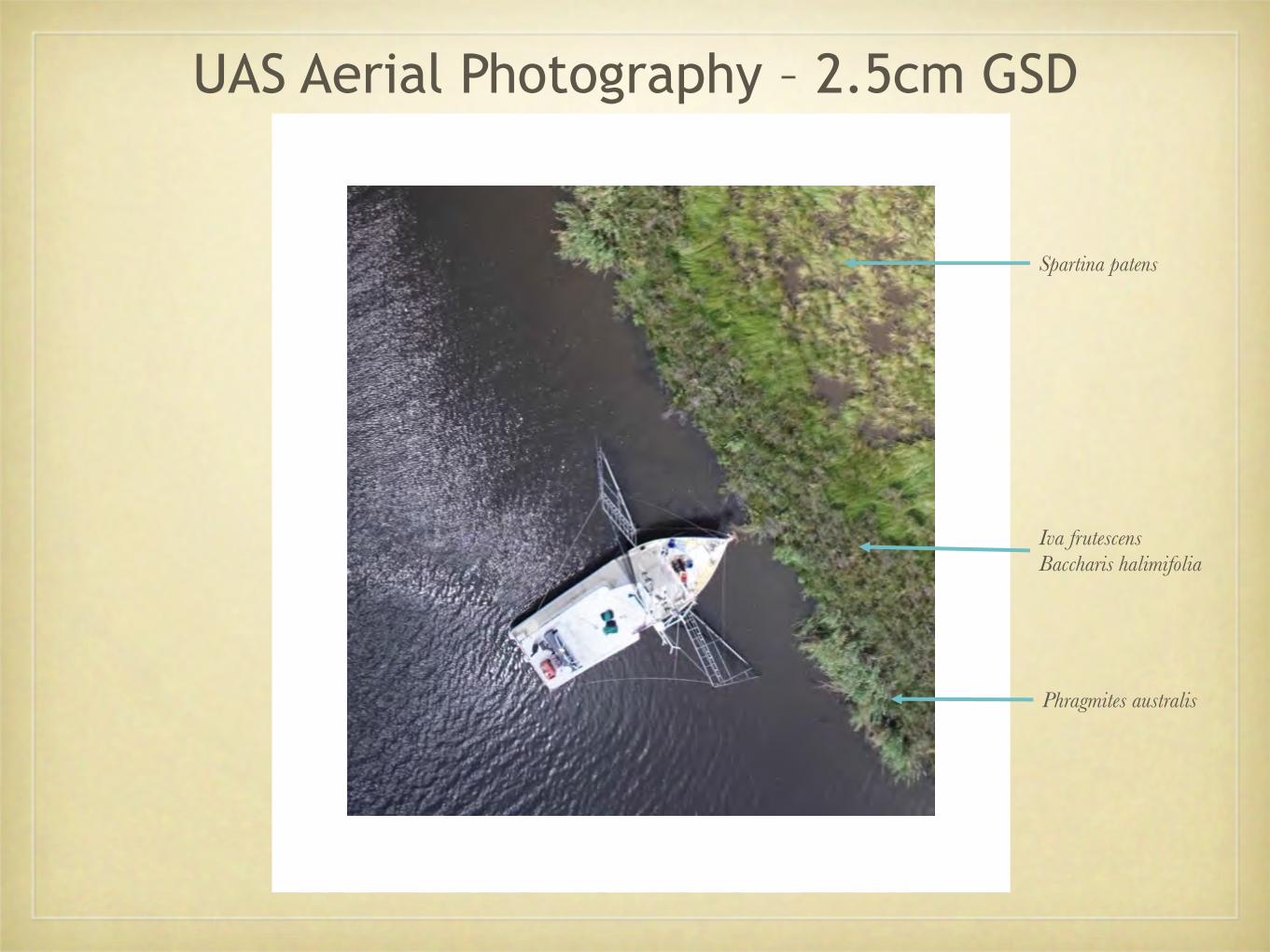
UAS Aerial Photography – 2.5cm GSD

Spartina patens

Phragmites australis

Iva frutescensBaccharis halimifolia

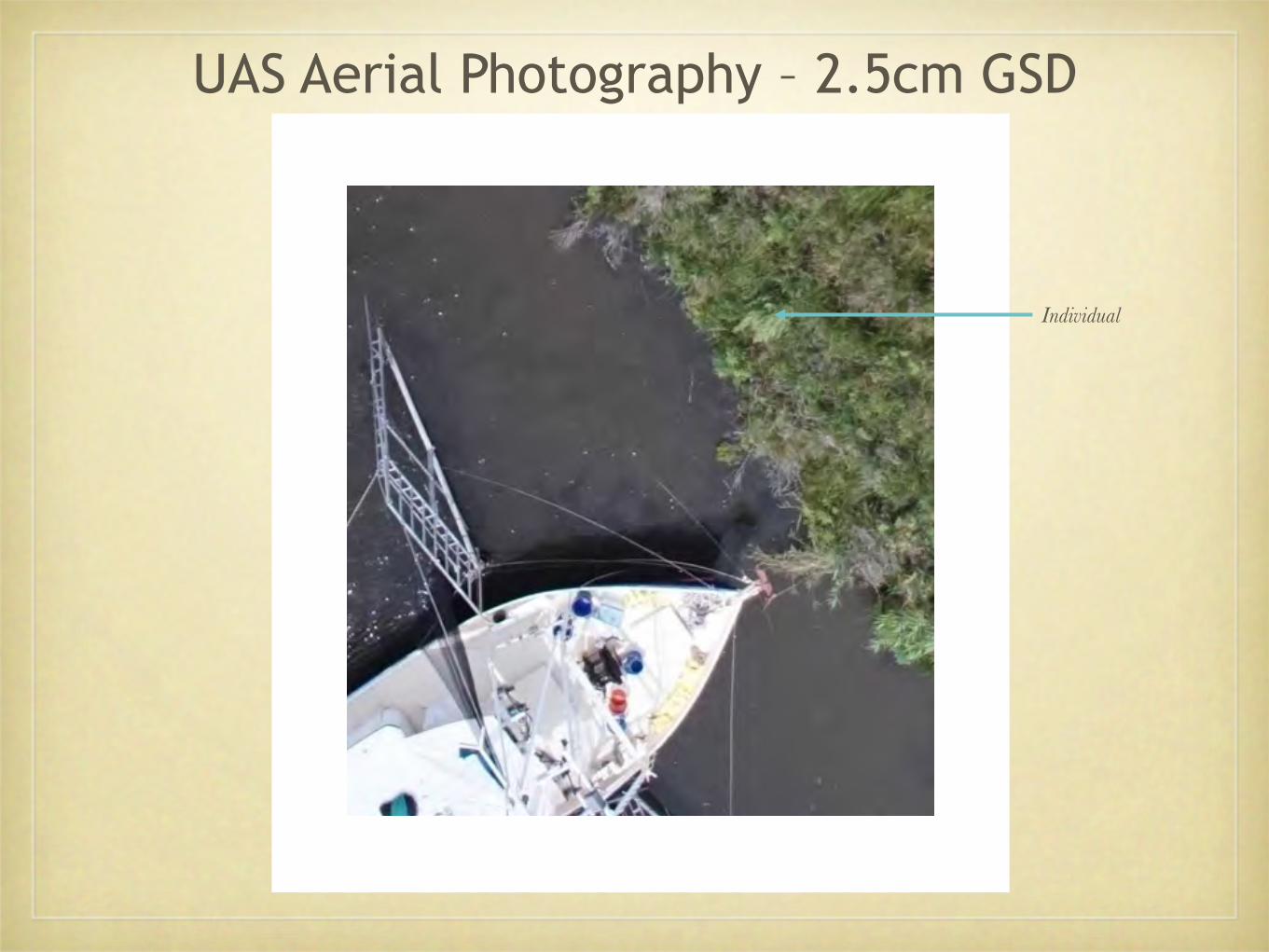
UAS Aerial Photography – 2.5cm GSD

Individual

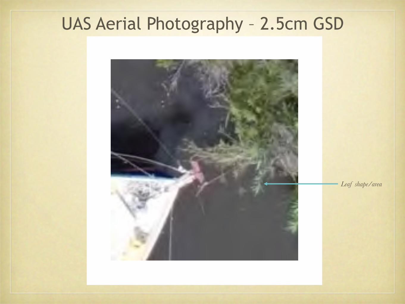
UAS Aerial Photography – 2.5cm GSD

Leaf shape/area

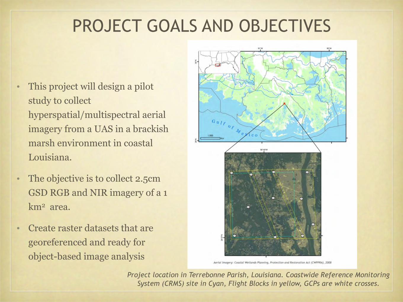
• This project will design a pilot study to collect hyperspatial/multispectral aerial imagery from a UAS in a brackish marsh environment in coastal Louisiana.

• The objective is to collect 2.5cm GSD RGB and NIR imagery of a 1 km2 area.

• Create raster datasets that are georeferenced and ready for object-based image analysis

PROJECT GOALS AND OBJECTIVES

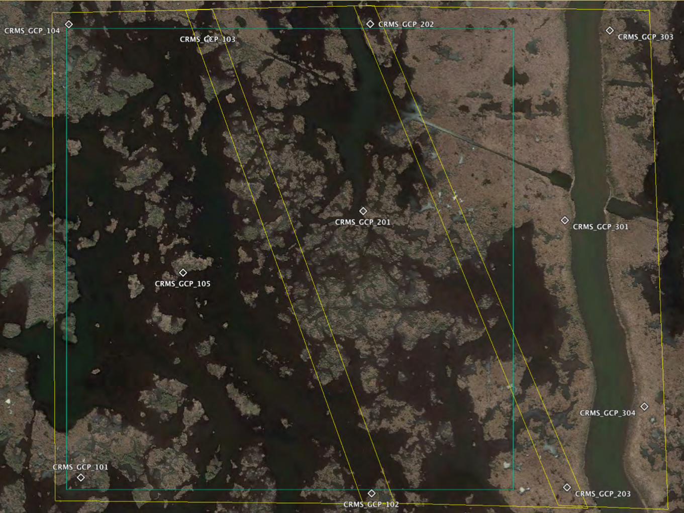
Project location in Terrebonne Parish, Louisiana. Coastwide Reference Monitoring System (CRMS) site in Cyan, Flight Blocks in yellow, GCPs are white crosses.

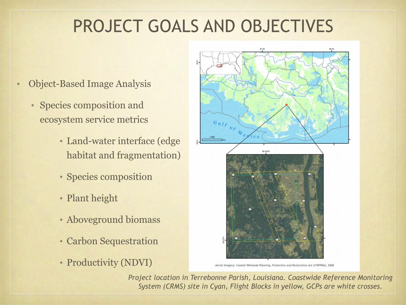
• Object-Based Image Analysis

• Species composition and ecosystem service metrics

• Land-water interface (edge habitat and fragmentation)

• Species composition

• Plant height

• Aboveground biomass

• Carbon Sequestration

• Productivity (NDVI)

PROJECT GOALS AND OBJECTIVES

Project location in Terrebonne Parish, Louisiana. Coastwide Reference Monitoring System (CRMS) site in Cyan, Flight Blocks in yellow, GCPs are white crosses.

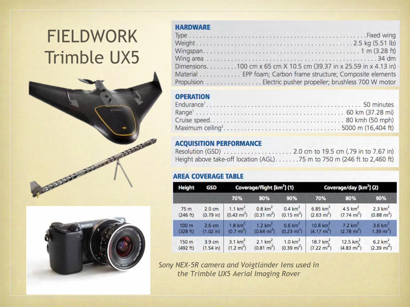
FIELDWORKTrimble UX5

Sony NEX-5R camera and Voigtlander lens used in the Trimble UX5 Aerial Imaging Rover

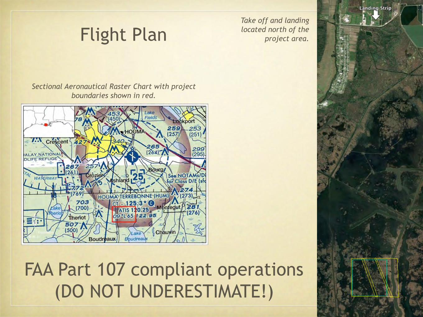
Flight Plan

Sectional Aeronautical Raster Chart with project boundaries shown in red.

Take off and landing located north of the

project area.

FAA Part 107 compliant operations(DO NOT UNDERESTIMATE!)

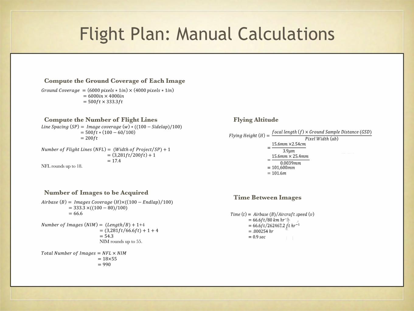
Flight Plan: Manual Calculations

!"#$%&' ) = +,%-'&./0'#%-' 1 ×( 100 − 789:%; 100) = 333.3×((100 − 80)/100) = 66.6

BC,$'#/D+,%-'& B+E = (F'8-Gℎ )) + 1+4

= (3,281DG 66.6DG) + 1 + 4 = 54.3 NIM rounds up to 55.

N/G%:BC,$'#/D+,%-'& = BOF×B+E

= 18×55 = 990

Compute the Ground Coverage of Each Image

Compute the Number of Flight Lines!"#$&'()"#* &+ = -.(*$)/0$1(*$ 2 ∗ ((100 − &"8$9(')/100)

= 500=> ∗ 100 − 60 100 = 200=>

AB.C$1/=D9"*ℎ>!"#$F AD! = (G"8>ℎ/=+1/H$)> &+) + 1 = 3,281=> 200=> + 1 = 17.4

NFL rounds up to 18.

Number of Images to be Acquired

Flying Altitude

Time Between Images

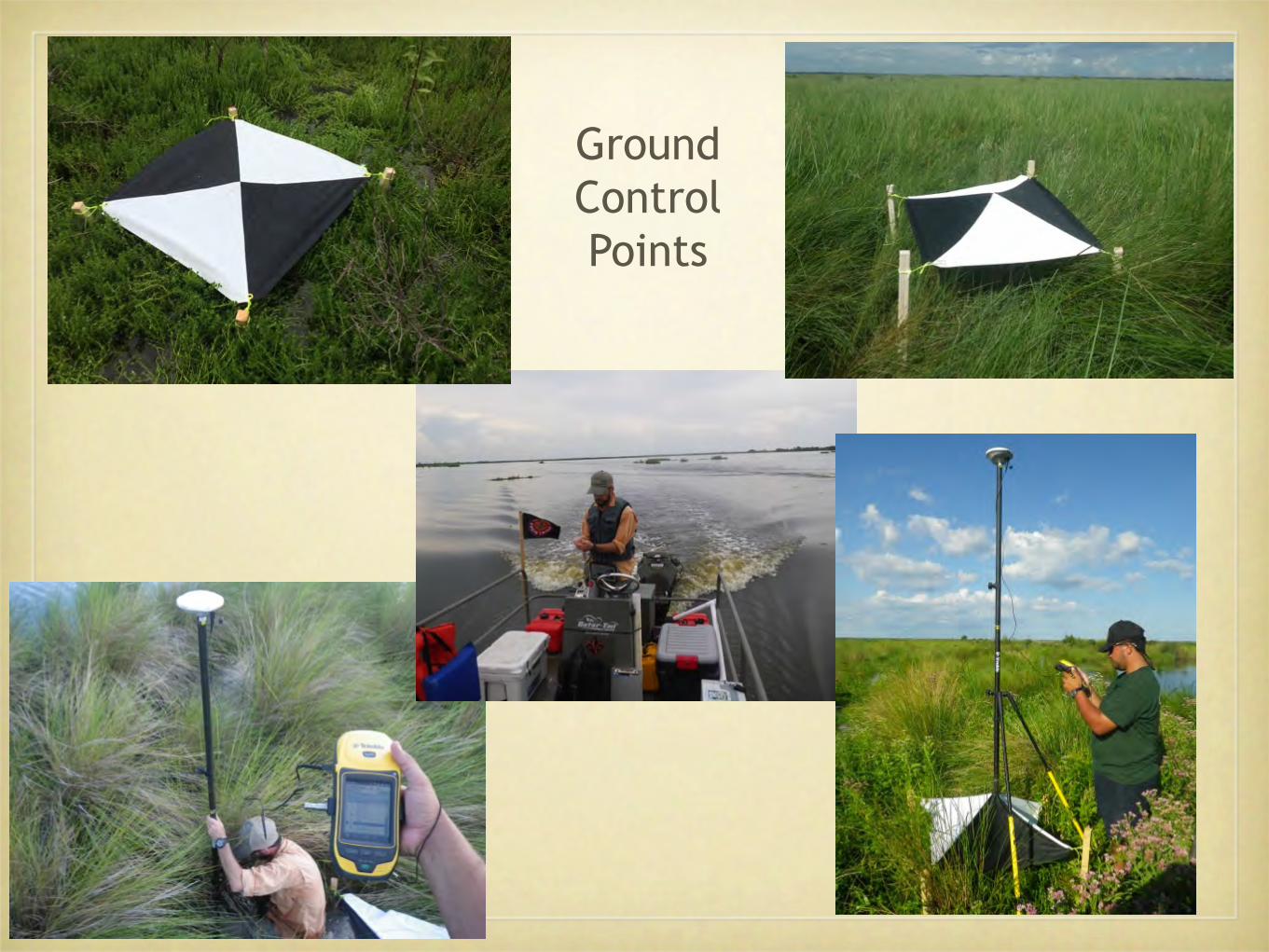
GroundControlPoints

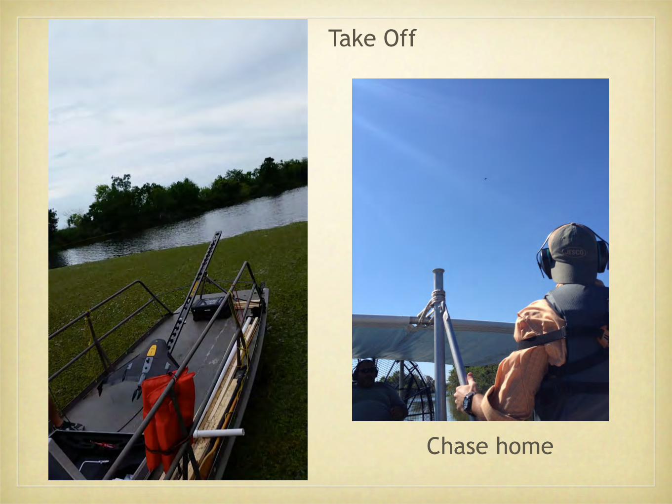
Take Off

Chase home

Belly land

Control Station

Post-Processing: Trimble UAS Master

A screenshot of the Basic Editor and the GCP/Manual Tie Point Table showing the location of a ground control point 20000 in image DSC01165_geotag.JPG.

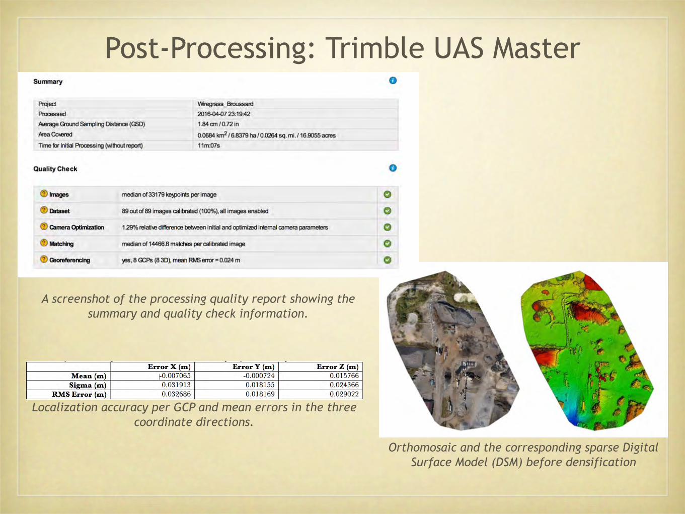
A screenshot of the processing quality report showing the summary and quality check information.

Orthomosaic and the corresponding sparse Digital Surface Model (DSM) before densification

Localization accuracy per GCP and mean errors in the three coordinate directions.

Post-Processing: Trimble UAS Master

Object Based Image Analysisi. Hyperspatial sub-decimeter imagery acquired using UAV platforms is

commonly analyzed using OBIA classification methods (e.g. Laliberte and Rango 2009, Laliberte and Rango 2011).

ii. For medium and low spatial resolution imagery acquired by satellites, such as Landsat or MODIS, the target is usually smaller than the pixel size. Pixel-based remote sensing classification schemes, like maximum likelihood classifiers that use spectral information, are often unsuitable for classifying hyperspatial data resulting in a lower overall classification accuracy (Blaschke 2010).

iii. As spatial resolution increases, variance in observed spectral values within target classes increases, making spectral separation between the classes more difficult to specify and classify (Marceau and Hay 1999, Blaschke 2010).

iv. OBIA methods address these scaling issues by segmenting the finer pixels into image objects that are made up of multiple neighboring pixels sharing similar spectral values (Blaschke, 2009)

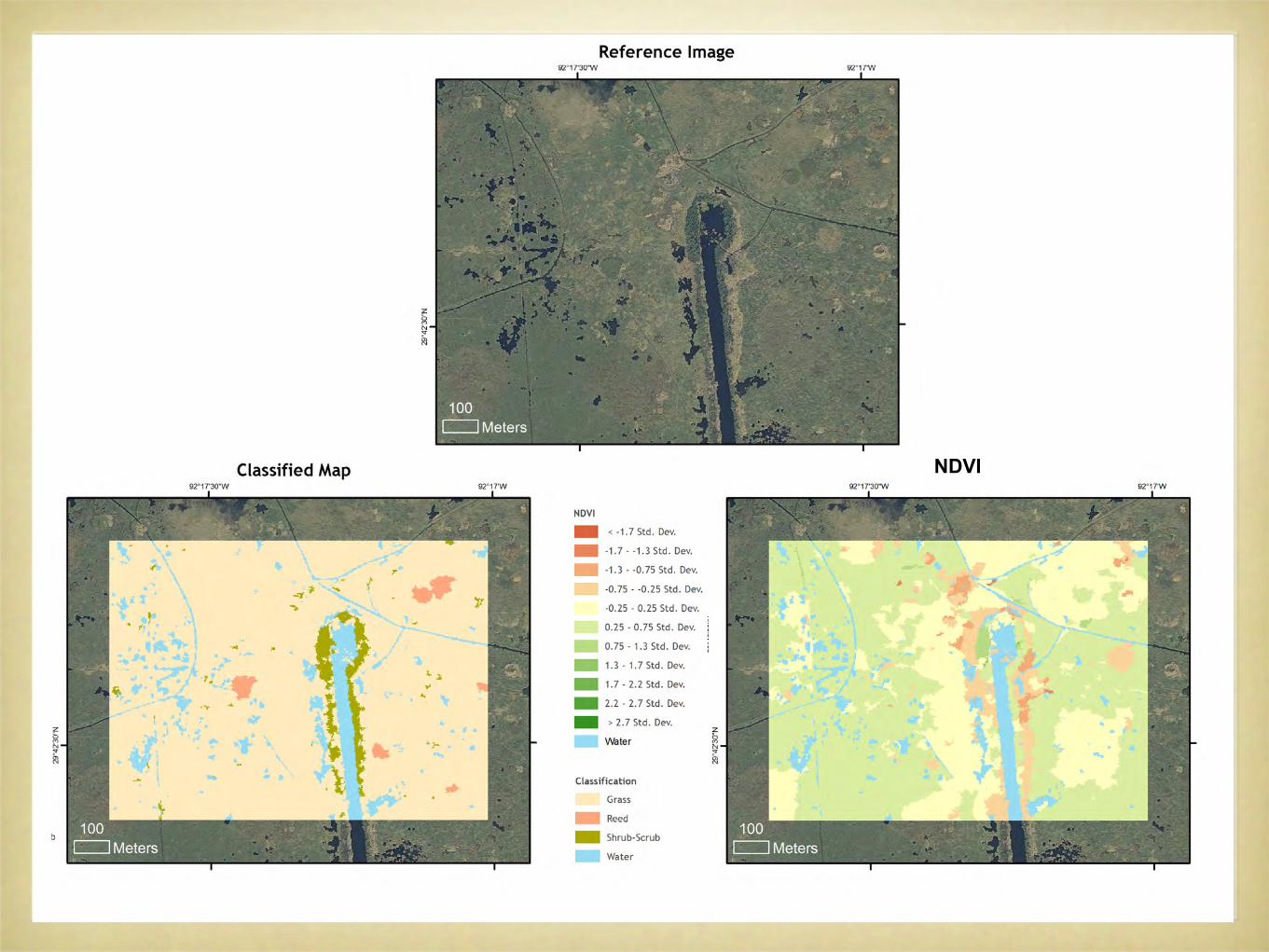
NDVI

NDVI

Workflow

OBIA

Land-water, species classes

with NDVI values and plant heights

Land-Water Classification

Explanation

Source data is Purple. Derived data is Green

Vector

Raster

Process

Table

UAS data collection

Dominant Species

Accuracy Assessment

NDVIPlant height

CRMS survey data

Biomass, C sequestration,

productivity

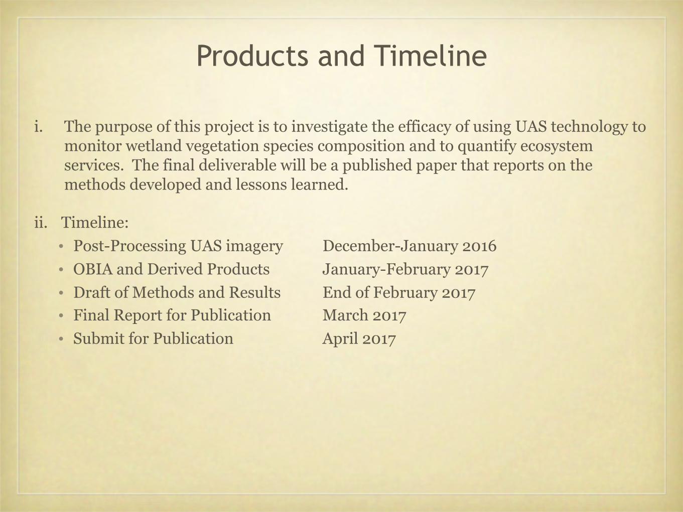
Products and Timeline

i. The purpose of this project is to investigate the efficacy of using UAS technology to monitor wetland vegetation species composition and to quantify ecosystem services. The final deliverable will be a published paper that reports on the methods developed and lessons learned.

ii. Timeline:• Post-Processing UAS imagery December-January 2016• OBIA and Derived Products January-February 2017• Draft of Methods and Results End of February 2017• Final Report for Publication March 2017• Submit for Publication April 2017

Blaschke, T. (2010). Object based image analysis for remote sensing. ISPRS Journal of Photogrammetry and Remote Sensing, 65(1), 2–16. Chong, A.K. (2007) HD aerial video for coastal zone ecological mapping. The 19th Annual Colloquium of the Spatial Information Research

Centre.Chust, G., et al. (2008). Coastal and estuarine habitat mapping, using LIDAR height and intensity and multi-spectral imagery. Estuarine, Coastal

and Shelf Science, 78(4), 633–643.Eisenbeiss, H., Lambers, K., & Sauerbier, M. (2005). Photogrammetric recording of the archaeological site of Pinchango Alto (Palpa, Peru) using a

mini helicopter (UAV). Annual Conference on Computer Applications and Quantitative Methods in Archaeology CAA, (March 2005), 21–24. Klemas, V. (2013). Airborne Remote Sensing of Coastal Features and Processes: An Overview. Journal of Coastal Research, 29(2), 239–255.Klemas, V. (2015). Coastal and Environmental Remote Sensing from Unmanned Aerial Vehicles: An Overview. Journal of Coastal Research,

315(5), 1260–1267. Laliberte, A. S., & Rango, A. (2009). Texture and scale in object-based analysis of subdecimeter resolution unmanned aerial vehicle (UAV)

imagery. IEEE Transactions on Geoscience and Remote Sensing, 47(3), 1–10. Laliberte, A. S., & Rango, A. (2011). Image Processing and Classification Procedures for Analysis of Sub-decimeter Imagery Acquired with an

Unmanned Aircraft over Arid Rangelands. GIScience & Remote Sensing, 48(1), 4–23.Laliberte, A. S., et al.. (2011). Multispectral remote sensing from unmanned aircraft: Image processing workflows and applications for rangeland

environments. Remote Sensing, 3(11), 2529–2551.Lechner, A. M., et al. (2012). Characterising Upland Swamps Using Object-Based Classification Methods and Hyper-Spatial Resolution Imagery

Derived From an Unmanned Aerial Vehicle. ISPRS Annals of Photogrammetry, Remote Sensing and Spatial Information Sciences, I-4(September), 101–106.

Marceau, D., and Hay, G. J (1999). Contributions of remote sensing to the scale issue. Canadian Journal of Remote Sensing, 25(4), 357–366.Niethammer, U., et al. (2012). UAV-based remote sensing of the Super-Sauze landslide: Evaluation and results. Engineering Geology, 128, 2–11. Phinn, S. R., et al. (1996). Monitoring Wetland Habitat Restoration in Southern California Using Airborne Multi spectral Video Data. Restoration

Ecology, 4(4), 412–422. Przybilla, H.-J., & Wester-Ebbinghaus, W. (1979). Bildflug mit ferngelenktem Kleinflug- zeug. Bildmessung Und Luftbildwesen Zeitschrift Fuer

Photogrammetrie Ferner- Kundung, 47(5), 137–142.Rocchini, D. (2007). Effects of spatial and spectral resolution in estimating ecosystem  diversity by satellite imagery. Remote Sensing of

Environment, 111(4), 423–434. Yang J., Artigas F. J., (2010) Mapping salt marsh vegetation by integrating hyperspectral and LiDAR remote sensing. In: Wang, J. (ed.). Remote

Sensing of Coastal Environments. Boca Raton, FL: CRC, pp. 173–190.

References

Whitney Broussardwbroussardiii@gmail.com