QUANTILE AND PROBABILITY CURVES WITHOUT CROSSING

QUANTILE AND PROBABILITY CURVES WITHOUT CROSSING

VICTOR CHERNOZHUKOV IVAN FERNANDEZ-VAL ALFRED GALICHON

Abstract. The commonly used approach in estimating conditional quantile curves is to

fit typically a linear curve pointwise for each quantile. This is done for a number of reasons:

linear models enjoy good approximation properties as well as have excellent computational

properties. The resulting fits may not respect a logical monotonicity requirement – that the

quantile curve, as a function of probability, should be monotone in that probability. This

paper studies the natural monotonization of these empirical curves induced by sampling

from the estimated non-monotone model, and then taking the resulting conditional quantile

curves, that by construction do not cross. This construction of monotone quantile curves

may be seen as a semi-parametric bootstrap and also as a monotonic rearrangement of

the original non-monotone function. These conditional quantile curves are monotone in

the probability and we show that, under correct specification, these curves have the same

asymptotic distribution as the original non-monotone curves. Thus, the empirical non-

monotone curves can be rearranged to be monotone without changing their (first order)

asymptotic distribution. However, this property does not hold under misspecification and

the asymptotics of these curves partially differs from the asymptotics of the original non-

monotone curves. Towards establishing the result, we establish the compact (Hadamard)

differentiability of the monotonized quantile and probability curves with respect to the

original curves. In doing so, we establish the results on the compact differentiability of

functions related to rearrangement operators. These results therefore generalize earlier

results on the compact differentiability of the inverse (quantile) operators.

Date: September 18, 2006.

1

CURVES WITHOUT CROSSING 1

1. Introduction

We can best describe the problem studied in this paper using linear quantile regression

models as the prime example. Suppose that x′β(u) is a linear approximation to the u-

quantile of real response variable Y given a vector of repressors X = x, for a given index

u. The typical approximations as well as estimation algorithms fit the conditional curve

x′β(u) pointwise in u ∈ (0, 1), producing an estimate β̂(u). The linear functional forms as

well as pointwise fitting are used for a number of reasons, including parsimony of resulting

approximation coupled with good computational properties. However, a problem that might

occur is that the map

u 7→ x′β̂(u)

may not be monotone in u, which violates the obvious logical requirement. In fact, the

non-monotonicity can occur due to either of the following reasons:

(1) (Monotonically correct case). The population curve u 7→ x′β(u) is increasing in

u, and thus satisfies the monotonicity requirement. However, the empirical curve

u 7→ x′β̂(u) is not monotone due to an estimation error.

(2) (Monotonically incorrect case). The population curve u 7→ x′β(u) is not monotone

due to imperfect approximation, and thus does not satisfy the monotonicity require-

ment. Therefore, the resulting empirical curve u 7→ x′β̂(u) is also not monotone due

to both estimation error and the non-monotonicity of the population curve.

Consider the function

F̂ (y|x) =∫ 1

01{x′β̂(u) ≤ y}du.

This function is monotone in y. Moreover, this is a proper distribution function of the

random variable

Yx := x′β̂(U) where U ∼ U(0, 1).

Hence

F̂−1(u|x) = inf{y : F̂ (y|x) ≥ u}

is monotone in u, hence this “rearranged” quantile curve is monotone in u, for each x. Thus,

starting with an original non-monotone curve u 7→ x′β̂(u), the rearrangement produces a

2 VICTOR CHERNOZHUKOV IVAN FERNANDEZ-VAL ALFRED GALICHON

monotone quantile curve F̂−1(u|x). This rearrangement mechanism has a direct relation

to the bootstrap, since the ”rearranged” quantile curve is produced by sampling from the

estimated original quantile model (cf. Koenker, 1994). This mechanism (and the name we

adopt for it) also has the direct relation to the “rearrangement mappings” in variational

analysis and operations research (e.g. Hardy et. al. (1953) and Villani (2003)).

The purpose of this paper is to establish the empirical properties of the corrected quantile

curve and its distribution curve:

u 7→ F̂−1(u|x) and u 7→ F̂ (u|x)

under scenarios (1) and (2). We will also look closely at the analytical properties of the

population curves: u 7→ F−1(u|x) and u 7→ F (u|x).

Towards describing the essence of the result, let us fix an x, and suppose that an estimate

of β̂(u) of β(u) is available that converges weakly to a Gaussian process:

√nx′(β̂(u)− β(u)) ⇒ x′G(u) (1.1)

in the metric space of bounded functions `∞(0, 1), e.g. under the conditions of Jureckova

(1992). Let F (y|x) :=∫ 10 1{x′β(u) ≤ y}du. The main result is that in the monotonically

correct case,√

n(F̂ (y|x)− F (y|x)) ⇒ F ′(y|x)[x′G(F (y|x))],

in metric space `∞(Y), where Y is the support of (Yx), and

F ′(y|x) =1

x′β′(u)

∣∣∣u=F (y|x)

.

This result follows by finding the Hadamard derivative, which is the main effort of the

paper, and then appealing to a delta method. Further, we show that

√n(F̂−1(u|x)− F−1(u|x)) ⇒ x′[G(u)]

in `∞((0, 1) × X ), which, remarkably, coincides with the asymptotics of the original curve

u 7→ x′β(u). This has a convenient practical implication: if the population curve is mono-

tone, then the empirical non-monotone curve can be re-arranged to be monotonic without

affecting its (first order) asymptotic properties. This result follows by finding the Hadamard

derivative, which is again the main effort of the paper, and then appealing to a delta method.


Further, the second result is that in the monotonically incorrect case,

√n(F̂ (y|x)− F (y|x)) ⇒

K(x,y)∑

k=1

x′G(uk(x, y))|x′β′(uk)|

where u1(x, y) < ... < uK(x, y) are solutions of equation y = x′β(u), assuming there is only

a finite number of them. This holds uniformly in (y, x) over appropriate sets defined in the

forthcoming section. Further,

√n(F̂−1(u|x)− F−1(u|x)) ⇒

( K(x,y)∑

k=1

1|x′β′(uk)|

)−1K(x,y)∑

k=1

x′G(uk(x, y))|x′β′(uk)| .

This result holds also holds uniformly in (u, x) over appropriate sets defined in the forth-

coming section.

Note that the same method also applies, with adaptation, to rearranging probability

distributions curves which are not monotonic. As discussed in detail in Section 3, the

monotone rearrangement on the quantile curve can also be done on a probability curve (by

exchanging the roles played by the quantile and the probability spaces). Suppose P̂ (y|x) is

a candidate estimate of a probability distribution curve which is not monotone. Consider a

rearranged monotone quantile curve associated with P̂ (y|x):

Q̂ (y|x) =∫ ∞

01{P̂ (y|x) < t}dy −

∫ 0

−∞1{P̂ (y|x) > t}dy

Then take the inverse of this quantile curve as the rearranged probability curve:

F (t|x) = inf {t : Q (t|x) ≥ y} ,

which is monotone. As it will be argued with more detail, a similar asymptotic distribution

theory goes through for Q̂ and F̂ . These results are useful in a variety of applications where

conditional distribution curves are estimated, but monotonicity does not hold due to the

pointwise nature of the approximations used, see for example Hall et. al. (1999).

Our results can be viewed as a general functional delta method for rearrangement op-

erators that include the inverse (quantile) operators as the special case. In this way our

results extend the previous results on compact differentiability of the quantile operators

by Gill and Johansen (1990) and Doss and Gill (1992) (see also the book by Dudley and

Norvaisa (1999) for an excellent treatment). Since the results on quantile operators have


seen numerous applications, we expect as many applications of the results on rearrangement

operators, especially in the regression context. There are many more potential applications

to the objects that are not probability or quantile curves, for example, demand curves and

production curves in economics, or growth curves in biometrics. In these applications, the

pointwise nature of fitting often introduces an error, which can be removed by the operation

of the rearrangement.

It can also be emphasized that since the results are given in terms of the differentiability

of the operator with respect to the basic estimated process, our results do not rely on

particular sampling properties or on a particular estimator being used. We also do not rely

on functional forms being linear (the previous discussion used them only as an example).

The only condition required is that a central limit theorem like (1.1) applies to the estimate

of a curve and that the population curves have some smoothness properties. Further, the

results do not rely on the exact nature of the population curve, for example, the results

do not depend on whether the underlying model is an ordinary or a structural quantile

regression model. Our results apply in either case without modification.

2. Quantile Curves without Crossing: Analytical and Empirical Properties

In this section, the treatment of the problem is somewhat more general than in the

introduction; namely, we replace the linear functional form x′β(u) by q(u, x). Define Yx =

Q(x,U) where U ∼ Uniform(U), where U = (0, 1), and let F (y|x) =∫ 10 1{Q(x, u) ≤ y}du

be the distribution function of Yx, and F−1(u|x) be the quantile function of Yx.

2.1. Basic Analytical Properties. In this section, we develop the basic properties of the

population objects F (y|x), its density f(y|x), and its inverse F−1(u|x).

We first recall the following basic definitions from Millnor (1965): Let g : U ⊂ R → R

a continuously differentiable function. A point x ∈ U is called a regular point of g if the

derivative of g at this point does not vanish, ie. g′ (x) 6= 0. A point x which is not a regular

point is called a critical point. A value y ∈ g (U) is called a regular value of g if g−1 ({y})contains only regular points, ie. if ∀x ∈ g−1 ({y}), g′ (x) 6= 0. A value y which is not a

regular value is called a critical value.


Denote Yx the support of Yx, and Y∗x be the subset of regular values of u 7→ Q(u, x)

in Yx. Denote XY = {(x, y) : x ∈ X , y ∈ Yx}, and XY∗ = {(x, y) : x ∈ X , y ∈ Y∗x}. We

assume throughout that Yx ⊂ Y, which is compact subset of R, and that x ∈ X , a compact

subset of Rd.

Introduce the following assumptions:

(a) Q(u, x) : U × X → R is a continuously differentiable function in both arguments,

(b) Q′(x, u) := ∂Q(u, x)/∂u does not vanish almost everywhere on U , for each x ∈ X ,

(c) the number of times ∂Q(u, x)/∂u changes its sign is bounded, uniformly in x ∈ X .

In some applications, the curves of interest are not functions of x, or we might be interested

in a particular value x. In this case, the set X is taken to be a singleton X = {x}.

Proposition 1 (Basic Properties of F (y|x), f(y|x), and F−1(y|x)). Under assumpions (a)

and (b), Let Y∗x be the subset of regular values of Q(u, x) in Yx, the support of Yx. The

basic properties of function F (y|x) are the following,

1. The set of non-regular values, Yx \ Y∗x, is finite, and∫Yx\Y∗x dF (y|x) = 0.

2. For any y ∈ Y∗x

F (y|x) =∫

Q(u,x)≤ydu =

K(y,x)∑

k=1

sign{Q′(uk(y, x), x)}uk(y, x) + 1{Q′(uK(y,x), x) < 0},

where {uk(y, x), for k = 1, ..., K(y, x) < ∞} are the roots of Q(u, x) = y in increasing

order.

3. For any y ∈ Y∗, the ordinary derivative f(y|x) = ∂F (y|x)/∂y exists, and its value is

f(y|x) =K(y,x)∑

k=1

1|Q′(uk(y, x), x)| ,

and it is continuous at each y ∈ Y∗x. F (y|x) is absolutely continuous in y ∈ Y and is strictly

increasing in y ∈ Y. Moreover, f(y|x) is a Radon-Nikodym derivative of F (y|x) with respect

to the Lebesgue measure.


4. The quantile function F−1(u|x) partially coincides with Q(u, x) on regions where the

latter function is increasing, namely

F−1(u|x) = Q(u, x),

provided u∗ = u is the unique solution of the equation F−1(u|x) = Q(u∗, x).

5. The quantile function F−1(u|x) is equivariant to location and scale transformations

of Q(x, u).

6. The quantile function F−1(u|x) has the ordinary derivative

1/f(F−1(u|x)|x),

when F−1(u|x) ∈ Y∗x, and 0 when F−1(u|x) ∈ Yx \ Y∗x, and the derivative is continuous.

This is also a Radon-Nikodym derivative with respect to the the Lebesgue measure.

7. The map (y, x) 7→ F (y|x) is continuous on YX and the map (u, x) 7→ F−1(u|x) is

continuous on UX .

The following synthetic simple example illustrates some of these basic properties in a

situation where the original quantile curve is chosen to be highly non monotone. Consider

the following hypothetical quantile function:

Q(u) = (4u− 2)3 − (4u− 2). (2.1)

Figure 1 shows that this function is non monotone. In particular, the slope of Q(u)

changes sign twice at .36 and .64 approximately. Figures 1 and 2 illustrate the second and

fourth results of the proposition by plotting together the original and rearranged quantile

and distribution curves. Here we can see that the rearranged functions are monotonically

increasing and coincide with the original ones for points where the initial distribution is

uniquely defined. For the rest of the points y, the rearranged distribution is a linear combi-

nation of the solutions to the equation Q(u) = y. The coefficients in this linear combination

alternate between 1 and -1 depending on whether the original quantile curve is increasing

or decreasing at the corresponding solution point.


Figures 2 illustrates the third and sixth results of the proposition by plotting the rear-

ranged density and sparsity curves. The density function is continuous at the regular values

of Q(u), and grows asymptotically to infinity at the critical values. Similarly, the sparsity

function is continuous at the regular points of Q(u), and takes the value zero at the critical

points.

2.2. Functional Derivatives. In this section, establish the Hadamard differentiability

of F (y|x) and F−1(y|x) with respect to Q(u, x), tangentially to the space of continuous

functions on U ×X . This differentiability property is important for statistical applications.

In what follows, `∞(U × X ) denotes the set of bounded and measurable functions h :

U × X → R, C(U × X ) denotes the set of continuous functions mapping h : U × X →R, and `1(U × X ) denotes the set of measurable functions h : U × X → R such that∫U

∫X |h(u, x)|dudx < ∞, where du and dx denote the integration with respect to the

Lebesgue measure on U and X , respectively.

Proposition 2. (Hadamard Derivative of F (y|x) with respect to Q(u, x)) Define F (y|x, ht) :=∫ 10 {Q(x, u) + tht(u, x) ≤ y}du. Under assumptions (a)-(c), as t → 0,

Dht(y, x, t) =F (y|x, ht)− F (y|x)

t→ Dh(y, x), (2.2)

Dh(y, x) := −K(y,x)∑

k=1

h(uk (y, x) , x)|Q′(uk(y, x), x)| . (2.3)

The convergence holds uniformly in any compact subset of YX ∗ := {(y, x) : y ∈ Yx, x ∈ X},for every |ht − h|∞ → 0, where ht ∈ `∞[U × X ], and h ∈ C(U × X ).

Proposition 3 (Hadamard Derivative of F−1(u|x) with respect to Q(u, x)). Under as-

sumptions (a) and (b) of Lemma 1, as t → 0,

D̃ht(u, x, t) :=F−1(u|x, ht)− F−1(u|x)

t→ D̃h(u, x), (2.4)

D̃h(u, x) := − 1f(F−1(u|x)|x)

·Dh(F−1(u|x), x), (2.5)

The convergence holds uniformly in any compact subsets of UX ∗ = {(u, x) : (F−1(u|x), x) ∈YX ∗}, for every |ht − h|∞ → 0, where ht ∈ `∞[U × X ], and h ∈ C(U × X ).


0 0.1 0.2 0.3 0.4 0.5 0.6 0.7 0.8 0.9 1−6

−4

−2

0

2

4

6

u

q(u)

F−1(u)

−6 −4 −2 0 2 4 60

0.1

0.2

0.3

0.4

0.5

0.6

0.7

0.8

0.9

1

y

q−1(y)F(y)

Figure 1. Left: “Approximate” quantile function Q(u) and the rearranged

quantile function. Right: “Approximate” distribution function Q−1(y) and

the rearranged distribution function F (y).

−6 −4 −2 0 2 4 60

0.5

1

1.5

y

f(y)

0 0.1 0.2 0.3 0.4 0.5 0.6 0.7 0.8 0.9 10

5

10

15

20

25

30

35

40

45

u

1/f(F−1(u))

Figure 2. Left: Density function f(y) of rearranged distribution function

F (y). Right: Density (sparsity) function the rearranged quantile function

F−1(u)).


The convergence holds uniformly on the regions that exclude the critical values of the

mapping u 7→ Q(u, x). At the critical values Q(u, x) possibly changes from increasing

to decreasing. Moreover, in the monotonically correct case, the following result is worth

emphasizing:

Corollary 1 (Monotonically correct case). Suppose u 7→ Q(u, x) has Q′(u, x) > 0 for each

x ∈ X then

Dht(y, x, t) → Dh(x, y)

uniformly in (y, x) ∈ YX , and

D̃ht(u, x, t) → D̃h(u, x)

uniformly in (u, x) ∈ UX .

Thus, the convergence is uniform over the entire domain in the monotonically correct

case. Regarding the monotonically incorrect case, a natural question that arises next is

whether by some operation of smoothing – namely integrating in y or x – we can achieve

the uniform convergence over the entire space. The answer appears positive in the case of

integrating in y, while some exclusions are needed in the case of integrating F (y|x) in x.

The following proposition calculates the Hadamard derivative of the following four func-

tionals obtained by integration:

(y′, x) 7→∫

Y1{y ≤ y′}g(y, x)F (y|x)dy, (y, x′) 7→

∫

X0

1{x ≤ x′}g(y, x)F (y|x)dx,

(u′, x) 7→∫

U1{u ≤ u′}g(u, x)F−1(u|x)du, (u, x) 7→

∫

X1{x ≤ x′}g(u, x)F−1(u|x)dx,

with restrictions on g and the set and the set X0 specified below in the statement of the

theorem. These elementary functionals are useful building blocks for various statistics, such

as Lorentz curves, means and other moments, as well as smoothed versions of curves F (y|x)

and F−1(y|x). For example, the conditional Lorentz curve is

L(u|x) =(∫

U1{u ≤ u′}F−1(u|x)du

)/( ∫

UF−1(u|x)du

),


which is a ratio of a partial mean to the mean. Hadamard differentiability of this statistic

with respect to the underlying Q(u, x) immediately follows from the Hadamard differentia-

bility of the elementary statistics above.

We need the following definitions for some of the results presented below. Let X o be a

region such that when X ′ ∼ Uniform(X0), Q(X ′, u) has a density denoted m(q|x) bounded

above uniformly in u. Note that this is not an assumption on the sampling behavior of

regressors, it is merely a definition of the region X0. In typical linear applications, X o

coincides with X if regressors are not redundant.1 Further let Y0 be a subset of Y such that∫X0

f(y|x)dx is bounded above for all y ∈ Y. It should be noted that the integral is finite

for almost every value of y, and thus Y0 may be smaller than Y.

Proposition 4. The following results are true with the limits being continuous on the

specified domains:

1.

∫

Y1{y ≤ y′}g(y, x)Dht(y, x, t)dy →

∫

Y1{y ≤ y′}g(y, x)Dh(y, x)dy

uniformly in (x, y′) ∈ X × Y, for any g ∈ `∞(YX ) such that x 7→ g(y, x) is continuous for

a.e. y.

2.

∫

X0

1{x ≤ x′}g(y, x)Dht(y, x, t)dx →∫

X0

1{x ≤ x′}g(y, x)Dh(y, x)dx

uniformly in (x′, y) ∈ X0 × Y0, for any g ∈ `∞(YX ) such that such that y 7→ g(y, x) is

continuous for a.e. x.

3.

∫

U1{u ≤ u′}g(u, x)D̃ht(u, x, t)du →

∫

U1{u ≤ u′}g(u, x)D̃h(u, x)dy

uniformly in (x, u′) ∈ X × U , for any g ∈ `1(UX ) such that x 7→ g(u, x) is continuous for

a.e. u.

4.

∫

X1{x ≤ x′}g(u, x)D̃ht(u, x, t)dx →

∫

X1{x ≤ x′}g(u, x)D̃h(u, x)dx

uniformly in (x′, u) ∈ X × U , for any g ∈ `1(UX ), such that u 7→ g(u, x) is continuous for

a.e. x.

1In the linear case ∂Q(u, x)/∂x = β−1(u).


This proposition essentially is a corollary of Proposition 4. Indeed, results (1)-(4) follow

from the fact that pointwise convergence of Proposition 3 coupled with uniform integrabil-

ity, shown in the proof of Proposition 4, allows to exchange limits and integration. Another

way of proving result (3) but not any other result in the paper can be based on exploiting

the convexity of the functional in (3) with respect to the underlying curve, following the

approach of Massino and Temam (1982) and Alvino et. al. (1990). Due to this limitation,

we did not follow this approach in this paper. However, details of this approach are de-

scribed in Chernozhukov, Fernandez-Val, and Galichon (2006) with an application to some

nonparametric estimation problems.

It is worthwhile emphasizing also the properties of the following functionals obtained by

applying a smoothing operator, denoted by S:

SF (y|x) =∫

kδ(y − y′)F (y′|x)dy′, kδ(v) = 1{|v| ≤ δ}/2δ,

SF−1(u|x) =∫

kδ(u− u′)F (u′|x)du′, kδ(v) = 1{|v| ≤ δ}/2δ.

Since these curves are merely formed as differences of the elementary functionals in Propo-

sition 4, parts (1) and (3), followed by a division by δ, the following corollary is immediate.

Corollary 2. We have that

SDht(y, x, t) → SDh(x, y)

uniformly in (y, x) ∈ YX , and

SD̃ht(u, x, t) → SD̃h(u, x)

uniformly in (u, x) ∈ UX .

Note that smoothing accomplishes uniform convergence over the entire domain, which is

a good property to have from the prospective of data analysis.

2.3. Empirical Properties of F̂ (y|x) and F̂−1(u, x). We are now ready to state the main

result for this section:


Proposition 5 (Empirical Properties of (y, x) 7→ F̂ (y|x) and (y, x) 7→ F̂−1(u, x)). Suppose

an estimate available such that Q̂(·, ·) takes its values in the space of bounded measurable

functions defined on U × X , and that in `∞(U × X )

√n(Q̂(x, u)−Q(x, u)) ⇒ G(u, x),

where G(x, u) is a Gaussian process with continuous paths. Suppose also that Q(x, u) sat-

isfies basic conditions (a),(b) and (c). Then in `∞(K), where K is any subset of YX ∗ that

is compact,√

n(F̂ (y|x)− F (y|x)) ⇒ DG(·,x)(y, x)

and in `∞(UXK) = {u : F−1(u|x) ∈ K, x ∈ X},

√n(F̂−1(u|x)− F−1(u|x)) ⇒ f(F−1(u|x)|x) ·DG(·,x)(F

−1(u|x), x).

Proposition 6 (Empirical Properties of Integrated Curves). Under the hypotheses of Propo-

sition 5, the following results are true with the limits being continuous on the specified

domains:

1.√

n

∫

Y1{y ≤ y′}g(y, x)(F̂ (y|x)− F (y|x))dy ⇒

∫

Y1{y ≤ y′}g(y, x)DG(y, x)dy

as stochastic processes indexed by (x, y′), in `∞(X × Y)

2.√

n

∫

X0

1{x ≤ x′}g(y, x)(F̂ (y|x)− F (y|x))dx ⇒∫

X0

1{x ≤ x′}g(y, x)DG(y, x)dx

as stochastic processes indexed by (x′, y), in `∞(X0 × Y0)

3.√

n

∫

U1{u ≤ u′}g(u, x)(F̂−1(u|x)− F−1(u|x))du ⇒

∫

U1{u ≤ u′}g(u, x)D̃G(u, x)dy

as stochastic processes indexed by (x, u′), in `∞(X × U)

4.√

n

∫

X1{x ≤ x′}g(u, x)(F̂−1(u|x)− F−1(u|x))dx ⇒

∫

X1{x ≤ x′}g(u, x)D̃G(u, x)dx

as stochastic processes indexed by (x′, u) in `∞(X × U). The restriction on function g are

as those specified in Proposition 4.


Corollary 3 (Large Sample Properties of Smoothed Curves). Under the hypotheses of

Proposition 5, in `∞(YX ),

√n(SF̂ (y|x)− SF (y|x)) ⇒ S[DG(·,x)(y, x)]

and in `∞(UX ),

√n(SF̂−1(u|x)− SF−1(u|x)) ⇒ S[f(F−1(u|x)|x) ·DG(·,x)(F

−1(u|x), x)],

3. Theory of Probability Curves without Crossing

The same method used here to monotonically rearrange quantile curves also applies

symmetrically to monotonically rearrange probability distribution curves, by a permutation

of the roles of the quantile and probability spaces.

There are several situations where one might be faced with the problem of non-increasing

probability curves. In an option pricing context, one could face situations similar to those

considered in Ait-Sahalia and Duarte (2003) where a ”risk-neutral distribution” is inferred

from some market data and due to some noise it is not completely monotonic. In some

situation, the probability distribution curve may have been obtained by some inverse trans-

formation and local non-monotonicity came as an artefact of the regularization technique.

In other situations, the particular smoothing technique may not respect monotonicity (see

Hall et. al. (1999) for a statement of this problem and various proposed solutions). Here we

propose to use the same method to rearrange the probability curves as we did for quantile

curves.

Suppose we have y 7→ P̂ (y) as a candidate empirical probability distribution curve, which

does not necessarily satisfy monotonicity. For the notational convenience we do not expose

the conditional case, which however goes through with an exact parallel as above. Define

the following quantile curve

Q̂(u) =∫ ∞

01{P̂ (y) < u}dy −

∫ 0

−∞1{P̂ (y) > u}dy

In what follows further assume support of P (y) is on Y ⊂ [0, +∞), so that the second term

drops down (otherwise it can be treated exactly in parallel to the first).


Consider also the inverse of the quantile curve is the rearranged probability curve

F̂ (y) = inf{

y : Q̂ (u) ≥ y}

.

which is monotone. It should be clear that the quantities Q̂ and F̂ play a role which is

exactly symmetric as the role played respectively by F̂ and Q̂ in the quantile case.

Therefore, if distribution curve (non necessarily monotonic) P (y) can be estimated using

an estimator P̂ such that√

n(P̂ (y)− P (y)

)⇒ G(y)

in `∞(Y), where G is a Gaussian process, one has in the monotonically correct case, that is

when P ′ (Q(u)) > 0 for all u ∈ [0, 1], that

√n

(Q̂(u)−Q(u)

)⇒

(1

P ′(Q(u))

)G (Q(u)) (3.1)

in `∞([0, 1]), and√

n(F̂ (y)− F (y)

)⇒ G (y) (3.2)

in `∞(Y).

Results paralleling those of the previous section are also obtainable for the monotonically

incorrect case:√

n(Q̂(u)−Q(u)

)⇒

K(u)∑

k=1

G (yk (u))|P ′(yk(u))| (3.3)

in `∞([0, 1]), and

√n

(F̂ (y)− F (y)

)⇒

K(u)∑

k=1

1|P ′(yk (u))|

−1

K(u)∑

k=1

G (yk (t))|P ′(yk (u))|

∣∣∣u=P (y)

(3.4)

in `∞(Y).

4. Illustrative Example: Engel Curves

To illustrate the application of our approach, we consider the estimation of expenditure

curves. We use the original Engel (1857) data to estimate the relationship between food

expenditure and annual household income. This is a classical data set in economics and is

based on 235 budget surveys of 19th century working-class Belgium households (see also


Koenker, 2005). The data were originally presented by Ernst Engel to support his hypothesis

that food expenditure constitutes a declining share of household income (Engel’s Law).

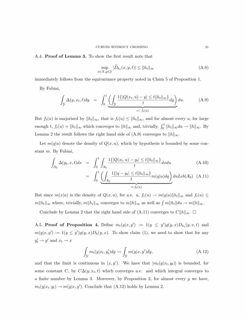
Figure 3 reproduces Figure A.1 in Koenker (2005). It shows a scatterplot of the En-

gel data on food expenditure vs. household income. Superimposed on the plot are the

{0.05, 0.1, 0.25, 0.75, 0.90, 0.95} quantile regression curves as dashed lines, together with the

median fit as a solid line. Here we can see that the quantile regression lines become closer as

we approach to the origin of the graph, indicating a potential problem of quantile crossing

for low values of income. This crossing problem of the Engel curves is more evident in

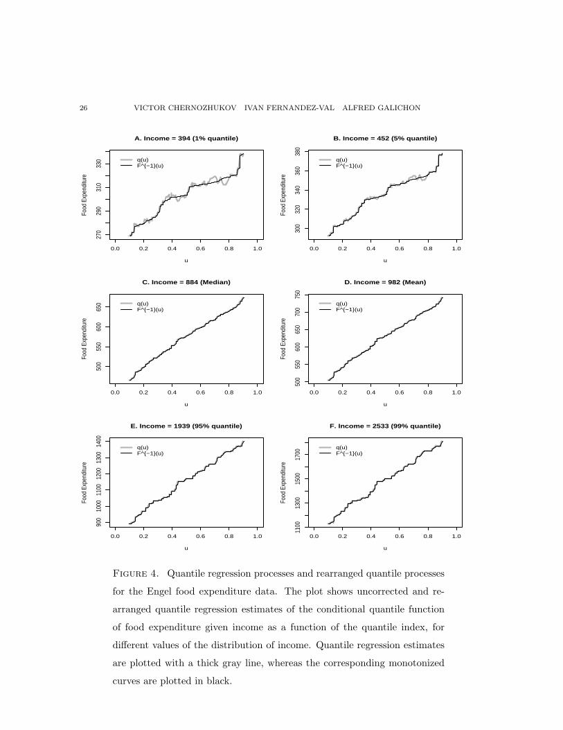
Figure 4, which plots the quantile regression process of food expenditure as a function of

the quantile index, instead of against the regressor. For low and very high quantiles of the

income, the quantile regression process, plotted as a thick gray line, is clearly non monotone.

Our rearrangement procedure fixes this undesirable feature of the quantile regression esti-

mates producing monotonically increasing quantile functions, which are plotted with black

lines in the figure. Moreover, the rearranged curves coincide with their quantile regression

counterparts for the middle and upper values of income where there is no quantile-crossing

problem.

Figure 5 illustrates how to perform quantile-uniform inference using the rearranged quan-

tile curves. It plots simultaneous 90% confidence intervals for the conditional quantile pro-

cess of food expenditure for two different values of income, the sample mean and the 1

percent sample percentile. The bands are constructed from both quantile regression, plot-

ted in light gray, and rearranged quantile curves, plotted in dark gray. A grid of quantiles

{0.10, 0.11, ..., 0.90} and 500 bootstrap repetitions are used to obtain the quantile regression

bands. For the rearranged curves, we assume that the estimand of the quantile regression

process is monotone and derive the bands using Lemma 1. As a result of this lemma,

bootstrap critical values for quantile regression are also valid for the rearranged curves,

what greatly reduces the computation time since we do not need to rearrange the curves in

each bootstrap iteration. The figure shows that even for the lower value of income there is

important overlapping between the bands for all the quantiles considered. This observation

points towards the maintained assumption that in this case the lack of monotonicity of the

quantile regression process is caused by sampling error due to the small sample size.


Appendix A. Proofs

A.1. Proof of Proposition 1. At first note that the distribution of Yx has no atoms.

Pr[Yx = y] = Pr[Q(U, x) = y] = Pr[U ∈ { roots of Q(u, x) = y}] = 0,

since the number of roots of Q(u, x) = y is finite under (a) and (b). Further, by assumptions

(a) and (b) the number of critical values of Q(x, u) is clearly finite, hence the claim (1)

follows.

For any regular y, letting u0(y, x) := 0

∫ 1

01(Q(u, x) ≤ y)du =

K(y,x)−1∑

k=0

∫ uk+1(y,x)

uk(y,x)1(Q(u, x) ≤ y)du +

∫ 1

uK(y,x)(y,x)1(Q(u, x) ≤ y)du.

Note that the signs of of Q′(u, x) alternate over consecutive uk(y, x)’s, determining whether

1{Q(y, x) ≤ y} = 1 on the interval [uk−1(y, x), uk(y, x)] (with u0(y, x) := 0), thus the

first term in the expression above simplifies to∑K(y,x)−1

k=0 1(Q′(uk+1, x) ≥ 0)(uk+1(y, x) −uk(y, x)); while the last term simplifies to 1(Q′(uK(y,x), x) ≤ 0)(1 − uK(y,x)). A further

simplification yields the expression given in the proposition.

The proof of (3) follows by taking the derivative of expression in (2), noting that at any

regular value y, the number of solutions K(y, x) is locally constant, and so are sign(u′k(y, x)),

moreover,

u′k(y, x) =sign(u′k(y, x))|Q′(uk(y, x), x)| .

Combining this fact with claim (2), we get the value of the derivative as in claim (3).

To show absolute continuity of F (y|x) with f(y|x) being the Radon-Nykodym derivative,

it suffices to show that for each y′,∫ y′∞ f(y|x)dx =

∫ y′−∞ dF (y|x), cf. Theorem 31.8 in (?).

Let V xt be the union of closed balls of radius t centered on the critical points Yx \ Y∗x, and

define Ytx = Yx\V x

t . Then,∫ y′−∞ 1{y ∈ Yt

x}f(y|x)dx =∫ y′−∞ 1{y ∈ Yt

x}dF (y|x). As t → 0,∫ y′−∞ 1{y ∈ Yt

x}dF (y|x) ↑ ∫ y′−∞ dF (y|x) by the set of critical critical points Yx\Y∗x being finite

and having mass zero under F (y|x). Therefore,∫ y′−∞ 1{y ∈ Yt

x}f(y|x)dx ↑ ∫ y′−∞ f(y|x)dx =

∫ y′−∞ dF (y|x).


Claim (4) follows by noting that at the regions where s → Q(s, x) is increasing and

one-to-one, and one has F (y|x) =∫Q(s,x)≤y ds =

∫s≤Q−1(y,x) ds = Q−1(y, x). Inverting the

equation u = F (F−1(u|x)|x) = Q−1(F−1(u|x), x) yields F−1(u|x) = Q(u, x).

Claim (5). We have Yx = Q(U, x) has quantile function F−1(u|x). The quantile function

of α + βQ(U, x) = α + βYx, for β > 0, is therefore inf{y : P (α + βYx ≤ y) ≥ u} =

α + βF−1(u|x).

Claim (6) is immediate from claim (3).

Claim (7). The proof of continuity of F (y|x) is subsumed in the proof of Proposition 3.

So we have that F (y|xt) → F (y|x) uniformly in y, and F (y|x) is continuous. Let ut → u

and xt → x. Since F (y|x) = u has a unique root y = F−1(u|x), the root of F (y|xt) = ut,

i.e. yt = F−1(yt|xt), converges to y, by the standard argument. ¤

A.2. Proof of Propositions 2-5. In the proofs that follow we will repeatedly use the

equivalence of the continuous convergence and the uniform convergence:

Lemma 1. Let D and D′ be complete separable metric spaces, and D is compact. Suppose

f : D → D′ is continuous. Then a sequence of functions fn : D → D′ converges to f

uniformly on D if and only if for any convergent sequence xn → x in D we have that

fn(xn) → f0(x).

Proof of Lemma 1: See, for example, Resnick, 1987, page 2.

Proof of Proposition 2. We have that for any δ > 0, there exists ε > 0 such that for

u ∈ Bε(uk(y, x)) for all small enough t ≥ 0

1{Q(x, u) + tht(u, x) ≤ y} ≤ 1{Q(x, u) + t(h(uk(y, x), x) + δ) ≤ y},

for all k ∈ 1, ..., K(y, x), and for all u 6∈ ∪kBε(uk(y, x))

1{Q(x, u) + tht(u, x) ≤ y} = 1{Q(x, u) ≤ y}.


Therefore,∫ 10 1{Q(x, u) + tht(u, x) ≤ y}du− ∫ 1

0 1{Q(x, u) ≤ y}du

t(A.1)

≤K(y,x)∑

k=1

∫

Bε(uk(y,x))

1{Q(x, u) + t(h(uk(y, x), x) + δ) ≤ y} − 1{Q(x, u) ≤ y}t

du

but by the change of variables this is equal to

K(y,x)∑

k=1

∫

Jk∩[y−t[h(uk(y,x),x)+δ],y]

1|Q′(Q−1(y′|x)|x)|dy,

where Jk is the image of Bε(uk(y, x)) under u 7→ Q(·, x). The change of variables is possible

because for ε small enough, Q(·, x) is one-to-one between Bε(uk(y, x)) and Jk.

For t small enough, we have that

Jk ∩ [y − t[h(uk(y, x), x) + δ], y] = [y − t[h(uk(y, x), x) + δ], y],

and

|Q′(Q−1(y′, x), x)| → |Q′(uk(y, x), x)|

as Q−1(y′, x) → uk(y, x). Therefore, the right hand term in (A.1) is less than

K(y,x)∑

k=1

−h(uk(y, x), x) + δ

|Q′(uk(y, x), x)| + o (1) .

Similarly∑K(y,x)

k=1−h(uk(y,x),x)−δ|Q′(uk(y,x),x)| + o (1) bounds (A.1) from below. Since δ > 0 can be made

arbitrarily small, the result follows.

It follows similarly that the result holds uniformly in (x, y) ∈ K, a compact subset of

YX ∗, as on such a set the functions (x, y) → |Q′(uk(y, x), x)| is uniformly continuous and

so is (x, y) 7→ K(y, x). To see the latter, note since K excludes a neighborhood of critical

points (Y \Y∗x, x ∈ X ), K is the union of a finite number of compact sets (K1, ...,KM ) over

any of which the function K(y, x) is constant: that is, K(y, x) = kj for some integer kj > 0,

for all (x, y) ∈ Kj , for all j ≤ M . ¤

Proof of Proposition 3. For a fixed x, Proposition 2, Step 1 of the proof below and an

application of the Hadamard differentiability of the quantile operator shown by [References]

give the result. The proof below, particularly Step 2, accommodates uniformity over x ∈ X .


Step 1. Let K be the subset of the set YX ∗. Let (yt, xt) be a convergent sequence

in this set, to a point, say (y, x). Then for every (yt, xt) → (y, x) we have for εt :=

‖ht‖∞ + ‖Q(xt, ·)−Q(x, ·)‖∞ + |yt − y| → 0 that

|F (yt|xt, ht)− F (y|x)| ≤∣∣∣∫ 1

01{Q(u, xt) + tht(u, x) ≤ yt}du− 1{Q(u, x) ≤ y}du

∣∣∣

≤∣∣∣∫ 1

01{|Q(x, u)− y| ≤ εt}du

∣∣∣ → 0, (A.2)

where the last step follows from the absolute continuity of F (y|x), the distribution function

of Q(U, x). This also verfies that F (y|x) is continuous in (y, x). This implies uniform con-

vergence of F (y|x, ht) to F (y, x) by Lemma 3. This in turn implies the uniform convergence

of quantiles F−1(u|x, ht) → F−1(u|x) uniformly over K, where K is any compact subset of

UX ∗.

Step 2. We have that uniformly over K,

(F (F−1(u|x, ht)|x, ht)− F (F−1(u|x, ht)|x))/t = Dh(F−1(u|x, ht), x) + o(1),

= Dh(F−1(u|x), x) + o(1),(A.3)

using Step 1 and Proposition 2, and using the continuity properties of Dh(y, x). Further,

uniformly over K, by Taylor expansion

F (F−1(u|x, ht)|x)− F (F−1(u|x)|x)t

∼ f(F−1(u|x)|x)F−1(u|x, ht)− F−1(u|x)

t(A.4)

and, as shown below,

F (F−1(u|x, ht)|x, ht)− F (F−1(u|x)|x)t

= o(1). (A.5)

Observe that the left hand side of (A.5) equals that of (A.4) plus that of (A.3). The result

follows.

It only remains to show equation (A.5) holds uniformly in K. Note that for any right-

continuous cdf F , we have that u ≤ F (F−1(u)) ≤ u + F (F−1(u)) − F (F−1(u)−), and for


any continuous, strictly increasing cdf F , we have that F (F−1(u)) = u. Therefore, write

0 ≤ F (F−1(u|x, ht)|x, ht)− F (F−1(u|x)|x)t

≤ u + (F (F−1(u|x, ht)|x, ht)− F (F−1(u|x, ht)− |x, ht)− u

t

≤ (F (F−1(u|x, ht)|x, ht)− F (F−1(u|x, ht)− |x, ht)t

(1)=

[F (F−1(u|x, ht)|x, ht)− F (F−1(u|x, ht)|x)]t

− [F (F−1(u|x, ht)− |x, ht)− F (F−1(u|x, ht)− |x)]t

(2)= (Dh(F−1(u|x, ht), x)−Dh(F−1(u|x, ht)−, x) + o(1) = o(1),

where in (1) we used that F (F−1(u|x, ht)|x) = F (F−1(u|x, ht)−|x) due to F (y|x) continuous

and strictly increasing in y, and in (2) we used Proposition 2. ¤

The following lemma due to Pratt (1960) will be useful.

Lemma 2. Let |fn| ≤ Gn and suppose that fn → f and Gn → G almost everywhere, then

if∫

Gn →∫

G finite, then∫

fn →∫

f .

A.3. Proof of Lemma 2. This lemma was proven by Pratt (1960). ¤

Lemma 3 (Boundedness and Integrability Properties). We have that for all x and y:

|D̃ht(u, x, t)| ≤ ‖ht‖∞ (A.6)

and

|Dht(y, x, t)| ≤ ∆(y, x, t) =∫ 1

0

1{|Q(x, u)− y| ≤ t‖ht‖∞}t

du, (A.7)

where for any xt → x ∈ X ,

∆(y, xt) → 2‖h‖∞f(y|x) for a.e y and∫

Y∆(y, xt, t)dy → ‖h‖∞

and for some constant C, for any yt → y ∈ Y0,

∆(yt, x) → 2‖h‖∞f(y|x) for a.e x in X0 and∫

X0

∆(yt, x, t)dx → ‖h∞‖C.

A simple consequence of the uniform integrability and of Propositions 2 and 3 is the

following result:


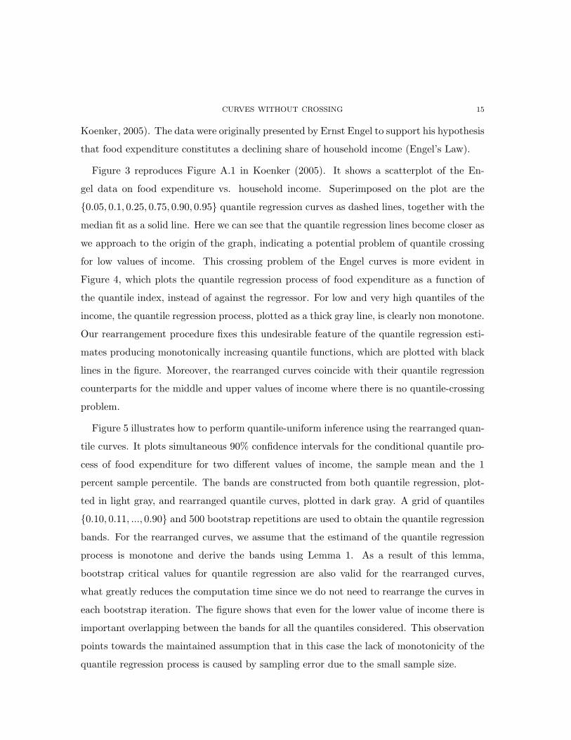
A.4. Proof of Lemma 3. To show the first result note that

supx∈X ,y∈Y

|D̃ht(x, y, t)| ≤ ‖ht‖∞ (A.8)

immediately follows from the equivariance property noted in Claim 5 of Proposition 1.

By Fubini,∫

Y∆(y, xt, t)dy =

∫ 1

0

(∫

Y

1{|Q(xt, u)− y| ≤ t‖ht‖∞}t

dy

)

︸︷︷︸=: ft(u)

du. (A.9)

But ft(u) is majorized by ‖ht‖∞, that is ft(u) ≤ ‖ht‖∞, and for almost every u, for large

enough t, ft(u) = ‖ht‖∞ which converges to ‖h‖∞ and, trivially,∫ 10 ‖ht‖∞du → ‖h‖∞. By

Lemma 2 the result follows the right hand side of (A.9) converges to ‖h‖∞.

Let m(q|u) denote the density of Q(x, u), which by hypothesis is bounded by some con-

stant m. By Fubini,∫

X0

∆(yt, x, t)dx =∫ 1

0

∫

X0

1{|Q(xt, u)− yt| ≤ t‖ht‖∞}t

dxdu (A.10)

=∫ 1

0

(∫

X0

1{|q − yt| ≤ t‖ht‖∞}t

m(q|u)dq

)

︸︷︷︸=:ft(u)

duLeb(X0) (A.11)

But since m(x|u) is the density of Q(x, u), for a.e. u, ft(u) → m(y|u)‖ht‖∞ and ft(u) ≤m‖ht‖∞ where, trivially, m‖ht‖∞ converges to m‖h‖∞ as well as

∫m‖ht‖du → m‖h‖∞.

Conclude by Lemma 2 that the right hand side of (A.11) converges to C‖h‖∞. ¤

A.5. Proof of Proposition 4. Define mt(y|x, y′) := 1(y ≤ y′)g(y, x)Dht(y, x, t) and

m(y|x, y′) := 1(y ≤ y′)g(y, x)Dh(y, x). To show claim (1), we need to show that for any

y′t → y′ and xt → x∫

Ymt(y|xt, y

′t)dy →

∫

Ym(y|x, y′)dy, (A.12)

and that the limit is continuous in (x, y′). We have that |mt(y|xt, yt)| is bounded, for

some constant C, by C∆(y, xt, t) which converges a.e. and which integral converges to

a finite number by Lemma 3. Moreover, by Proposition 2, for almost every y we have,

mt(y|xt, yt) → m(y|x, y′). Conclude that (A.12) holds by Lemma 2.


In order to check continuity, we need to show that for any y′t → y′ and xt → x

∫

Ym(y|x, y′)dy →

∫

Ym(y|x, y′)dy, (A.13)

We have that m(y|xt, y′t) → m(y|x, y′) for almost every y. Moreover, m(y|xt, yt) is domi-

nated by ‖g‖∞‖h‖∞f(y|xt), which converges to ‖g‖∞‖h‖∞f(y|x) for almost every y, and,

moreover,∫Y ‖g‖∞‖h‖∞f(y|x)dy converges to ‖g‖∞‖h‖∞. Conclude that (A.13) holds by

Lemma 2.

The proof of claim (2) follows similarly to the proof of claim (1).

[The part that follows can be omitted because it is also similar.]

To show claim (3), define mt(u|x, u′) = 1{u ≤ u′}g(u, x)D̃ht(u, x) and m(u|x, u′) = 1{u ≤u′}g(u, x)D̃h(u, x). To show claim (1), we need to show that for any u′t → u′ and xt → x

∫

Umt(u|xt, u

′t)dy →

∫

Um(u|x, u′)du, (A.14)

and that the limit is continuous in (x, u′). We have that mt(u|xt, u′t) is bounded by

g(u, xt)‖ht‖∞, which converges to g(u, x)‖h‖∞ for a.e. u, and which integral converges

to that of g(u, x)‖h‖∞ by the dominated convergence theorem. Moreover by Proposition

2, for almost every u we have mt(u|xt, u′t) → m(u|x, u′). Conclude that (A.14) holds by

Lemma 2.

In order to check continuity, we need to show that for any u′t → u′ and xt → x

∫

Um(u|x, u′t)du →

∫

Um(u|x, u′)du, (A.15)

We have that m(u|xt, u′t) → m(u|x, u′) for almost every u. Moreover, for small enough t,

m(u|xt, u′t) is dominated by |g(u, xt)|‖h‖∞, which converges for almost every value of u and

which integral converges by dominated convergence theorem. Conclude that (A.15) holds

by Lemma 2.

The proof of claim (4) follows similarly to the proof of claim (3). ¤

A.6. Proof of Proposition 5. This simply follows by the delta method (Van der Vaart,

1998). Here we remind ourselves what it is. To show the first part, consider the map

gn(h) = n−1/2(F (y|x, n−1/2h)−F (y|x). The sequence of maps satisfies gn′(hn′) → Dh(x, y)


for every subsequence hn′ → h in `∞(UX ∗), where h is continuous. It follows by the extended

continuous mapping theorem that gn(√

n(q̂(u, x)−Q(u, x))) ⇒ DG(·,x)(y, x). Conclude sim-

ilarly for the second part. ¤

A.7. Proof of Proposition 6. This follows by the delta method. ¤

References

[1] Ait-Sahalia, Y. and Duarte, J., ”Nonparametric option pricing under shape. restrictions,” Journal of

Econometrics 116, pp. 9–47, 2003.

[2] Alvino, A., Lions, P. L. and Trombetti, G., ”On Optimization Problems with Prescribed Rearrange-

ments,” Nonlinear Analysis 13 (2), pp. 185–220, 1989.

[3] Doss, Hani; Gill, Richard D. An elementary approach to weak convergence for quantile processes, with

applications to censored survival data. J. Amer. Statist. Assoc. 87 (1992), no. 419, 869–877.

[4] Dudley, Richard M.; Norvaisa, Rimas Differentiability of six operators on nonsmooth functions and p-

variation. With the collaboration of Jinghua Qian. Lecture Notes in Mathematics, 1703. Springer-Verlag,

Berlin, 1999. viii+277 pp.

[5] Fan, J., Yao, Q., and Tong, H., “Estimation of conditional densities and sensitivity measures in. non-

linear dynamical systems,” Biometrika, 83, pp. 189–206, 1996.

[6] Gill, Richard D.; Johansen, Soren. A survey of product-integration with a view toward application in

survival analysis. Ann. Statist. 18 (1990), no. 4, 1501–1555.

[7] Hall, P., Wolff, R., and Yao, Q., ”Methods for estimating a conditional distribution function,” Journal

of the American Statistical Association 94, pp. 154–163, 1999.

[8] Hardy, G., Littlewood, J., and Polya, G., Inequalities, Cambridge: Cambridge University Press, 1952.

[9] Koenker, Roger Confidence intervals for regression quantiles. Asymptotic statistics (Prague, 1993),

349–359, Contrib. Statist., Physica, Heidelberg, 1994

[10] Koenker, R. (2005) Quantile Regression, Econometric Society Monograph Series, Cambridge University

Press.

[11] Milnor, J., Topology from the differential viewpoint, Princeton University Press, 1965.

[12] Mossino J. and Temam, R. , ”Directional derivative of the increasing rearrangement mapping and

application to a queer differential equation in plasma physics,” Duke Math. J. 48 (3), 475–495, 1981.

[13] Pratt, J.W.: On interchanging limits and integrals. Ann. Math. Stat. 31, 74 (1960)

[14] Rudin, W., Functional Analysis, 2nd edition, New York: McGraw-Hill, Inc., 1991.

[15] Vaart, A. van der, Wellner, J., Weak convergence and empirical processes: with applications to statistics,

New York: Springer, 1996.

[16] Villani, C., Topics in Optimal Transportation, Providence: American Mathematical Society, 2003.


[17] van der Vaart, A. W. Asymptotic statistics. Cambridge Series in Statistical and Probabilistic Mathe-

matics, 3. Cambridge University Press, Cambridge, 1998. xvi+443 pp


1000 2000 3000 4000 5000

500

1000

1500

2000

Income

Food

Exp

endi

ture

Figure 3. Scatterplot and quantile regression fit of the Engel food ex-

penditure data. The plot shows a scatterplot of the Engel data on

food expenditure vs. household income for a sample of 235 19th cen-

tury working-class Belgium households. Superimposed on the plot are the

{0.05, 0.10, 0.25, 0.75, 0.90, 0.95} quantile regression curves as dashed lines,

and the median fit as a solid line.


0.0 0.2 0.4 0.6 0.8 1.0

270

290

310

330

u

Food

Exp

endi

ture

A. Income = 394 (1% quantile)

q(u)F^{−1}(u)

0.0 0.2 0.4 0.6 0.8 1.0

300

320

340

360

380

u

Food

Exp

endi

ture

B. Income = 452 (5% quantile)

q(u)F^{−1}(u)

0.0 0.2 0.4 0.6 0.8 1.0

500

550

600

650

u

Food

Exp

endi

ture

C. Income = 884 (Median)

q(u)F^{−1}(u)

0.0 0.2 0.4 0.6 0.8 1.0

500

550

600

650

700

750

u

Food

Exp

endi

ture

D. Income = 982 (Mean)

q(u)F^{−1}(u)

0.0 0.2 0.4 0.6 0.8 1.0

900

1000

1100

1200

1300

1400

u

Food

Exp

endi

ture

E. Income = 1939 (95% quantile)

q(u)F^{−1}(u)

0.0 0.2 0.4 0.6 0.8 1.0

1100

1300

1500

1700

u

Food

Exp

endi

ture

F. Income = 2533 (99% quantile)

q(u)F^{−1}(u)

Figure 4. Quantile regression processes and rearranged quantile processes

for the Engel food expenditure data. The plot shows uncorrected and re-

arranged quantile regression estimates of the conditional quantile function

of food expenditure given income as a function of the quantile index, for

different values of the distribution of income. Quantile regression estimates

are plotted with a thick gray line, whereas the corresponding monotonized

curves are plotted in black.


0.0 0.2 0.4 0.6 0.8 1.0

200

250

300

350

400

u

Food

Exp

endi

ture

A. Income = 394 (1% quantile)

q(u)F^{−1}(u)q(u)F^{−1}(u)

0.0 0.2 0.4 0.6 0.8 1.0

400

500

600

700

800

u

Food

Exp

endi

ture

B. Income = 982 (Mean)

q(u)F^{−1}(u)q(u)F^{−1}(u)

Figure 5. Simultaneous 90% confidence bands for quantile regression pro-

cesses and rearranged quantile processes for the Engel food expenditure data.

The figure shows quantile-uniform bands for uncorrected and rearranged

quantile regression estimates of the conditional quantile function of food ex-

penditure given income as a function of the quantile index, for two different

values of the distribution of income. Quantile regression bands are plotted

in light gray, whereas the corresponding monotonized bands are in dark gray.

Documents

QUANTILE AND PROBABILITY CURVES WITHOUT CROSSING