Munich Personal RePEc Archive

Quantile-Based Nonparametric Inference

for First-Price Auctions

Marmer, Vadim and Shneyerov, Artyom

University of British Columbia

October 2006

Online at https://mpra.ub.uni-muenchen.de/5899/

MPRA Paper No. 5899, posted 23 Nov 2007 06:12 UTC

Quantile-Based Nonparametric Inference for

First-Price Auctions�

Vadim Marmer

University of British Columbia

Artyom Shneyerov

Concordia University

September 7, 2007

Abstract

We propose a quantile-based nonparametric approach to inference on the

probability density function (PDF) of the private values in �rst-price sealed-

bid auctions with independent private values. Our method of inference is based

on a fully nonparametric kernel-based estimator of the quantiles and PDF of

observable bids. Our estimator attains the optimal rate of Guerre, Perrigne, and

Vuong (2000), and is also asymptotically normal with the appropriate choice

of the bandwidth. As an application, we consider the problem of inference on

the optimal reserve price.

Keywords: First-price auctions, independent private values, nonparametric

estimation, kernel estimation, quantiles, optimal reserve price.

1 Introduction

Following the seminal article of Guerre, Perrigne, and Vuong (2000), GPV hereafter,

there has been an enormous interest in nonparametric approaches to auctions.1 By

removing the need to impose tight functional form assumptions, the nonparametric

approach provides a more �exible framework for estimation and inference. Moreover,

�We thank Don Andrews for helpful comments. Pai Xu provided excellent research assistance.The �rst author gratefully acknowledges the research support of the Social Sciences and HumanitiesResearch Council of Canada under grant number 410-2007-1998.

1See a recent survey by Athey and Haile (2005).

1

the sample sizes available for auction data can be su¢ciently large to make the non-

parametric approach empirically feasible.2 This paper contributes to this literature

by providing a fully nonparametric framework for making inferences on the density

of bidders� valuations f (v). The need to estimate the density of valuations arises

in a number of economic applications, as for example the problem of estimating a

revenue-maximizing reserve price.3

As a starting point, we brie�y discuss the estimator proposed in GPV. For the

purpose of introduction, we adopt a simpli�ed framework. Consider a random, i.i.d.

sample bil of bids in �rst-price auctions each of which has n bidders; l indexes auctions

and i = 1; : : : ; n indexes bids in a given auction. GPV assume independent private

values (IPV). In equilibrium, the bids are related to the valuations via the equilibrium

bidding strategy B: bil = B (vil). GPV show that the inverse bidding strategy is

identi�ed directly from the observed distribution of bids:

v = � (b) � b+1

n� 1

G (b)

g (b); (1)

where G (b) is the cumulative distribution function (CDF) of bids in an auction with

n bidders, and g (b) is the corresponding density. GPV propose to use nonparametric

estimators G and g. When b = bil, the left-hand side of (1) will then give what GPV

call the pseudo-values vil = � (bil). The CDF F (v) is estimated as the empirical

CDF, and the PDF f (v) is estimated by the method of kernels, both using vil as

observations. GPV show that, with the appropriate choice of the bandwidth, their

estimator converges to the true value at the optimal rate (in the minimax sense;

Khasminskii (1978)). However, the asymptotic distribution of this estimator is as

yet unknown, possibly because both steps of the GPV method are nonparametric

with estimated values vil entering the second stage, and because the GPV estimator

2For example, List, Daniel, and Michael (2004) study bidder collusion in timber auctions usingthousands of auctions conducted in the Province of British Columbia, Canada. Samples of similarsize are also available for highway procurement auctions in the United States (e.g., Krasnokutskaya(2003)).

3This is an important real-world problem that arises in the administration of timber auctions, forexample. The actual objectives of the agencies that auction timber may vary from country to country.In the United States, obtaining a fair price is the main objective of the Forest Service. As observed inHaile and Tamer (2003), this is a vague objective, and determining the revenue maximizing reserveprice should be part of the cost-bene�ts analysis of the Forest Service�s policy. In other countries,maximizing the expected revenue from each and every auction is a stated objective, as is for examplethe case for BC Timber Sales (Roise, 2005).

2

requires trimming.

The estimator f (v) proposed in this paper avoids the use of pseudo-values and

does not involve trimming; it builds instead on the insight of Haile, Hong, and Shum

(2003).4 They show that the quantiles of the distribution of valuations can be ex-

pressed in terms of the quantiles, PDF, and CDF of bids. We show below that this

relation can be used for estimation of f (v). Consider the � -th quantile of valuations

Q (�) and the � -th quantile of bids q (�). The latter can be easily estimated from

the sample by a variety of methods available in the literature. As for the quantile of

valuations, since the inverse bidding strategy � (b) is monotone, equation (1) implies

that Q (�) is related to q (�) as follows:

Q (�) = q (�) +�

(n� 1) g (q (�)); (2)

providing a way to estimate Q (�) by a plug-in method. The CDF F (v) can then be

recovered simply by inverting the quantile function, F (v) = Q�1 (v).

Our estimator f (v) is based on a simple idea that by di¤erentiating the quantile

function we can recover the density: Q0 (�) = 1=f (Q (�)), and therefore f (v) =

1=Q0 (F (v)). Taking the derivative in (2) and using the fact that q0 (�) = 1=g (q (�)),

we obtain, after some algebra, our basic formula:

f (v) =

�n

n� 1

1

g (q (F (v)))�

1

n� 1

F (v) g0 (q (F (v)))

g3 (q (F (v)))

��1: (3)

Note that all the quantities on the right-hand side, i.e. g (b), g0 (b), q (�), F (v) =

Q�1 (v) can be estimated nonparametrically, for example, using kernel-based methods.

Once this is done, we can plug them in (3) to obtain our nonparametric estimator.

The expression in (3) can be also derived the relationship between the CDF of

values and the CDF of bids:

F (v) = G (B (v)) :

Applying the change of variable argument to the above identity, one obtains

f (v) = g (B (v))B0 (v)

4The focus of Haile, Hong, and Shum (2003) is a test of common values. Their model is thereforedi¤erent from the IPV model, and requires an estimator that is di¤erent from the one in GPV. Seealso Li, Perrigne, and Vuong (2002).

3

= g (B (v)) =�0 (B (v))

=

�n

n� 1

1

g (B (v))�

1

n� 1

F (v) g0 (B (v))

g3 (B (v))

��1:

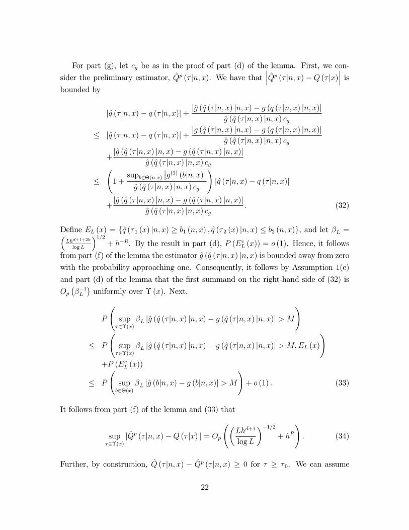
Note however, that, from the estimation perspective, the quantile-based formula ap-

pears to be more convenient, since the bidding strategy functionB involves integration

of F (see GPV). Furthermore, as we show below, quantile-based approach eliminates

trimming, which is likely to be one of the factors preventing one from establishing

asymptotic normality of the GPV estimator.

Our framework results in the estimator of f (v) that is both consistent and asymp-

totically normal, with an asymptotic variance that can be easily estimated. Moreover,

we show that, with an appropriate choice of the bandwidth sequence, the proposed

estimator attains the minimax rate of GPV.

As an application, we consider the problem of inference on the optimal reserve

price. Several previous articles have considered the problem of estimating the optimal

reserve price. Paarsch (1997) develops a parametric approach and applies his esti-

mator to timber auctions in British Columbia. Haile and Tamer (2003) consider the

problem of inference in an incomplete model of English auction, derive nonparamet-

ric bounds on the reserve price and apply them to the reserve price policy in the US

Forest Service auctions. Closer to the subject of our paper, Li, Perrigne, and Vuong

(2003) develop a semiparametric method to estimate the optimal reserve price. At

a simpli�ed level, their method essentially amounts to re-formulating the problem

as a maximum estimator of the seller�s expected pro�t. Strong consistency of the

estimator is shown, but its asymptotic distribution is as yet unknown.

In this paper, we propose asymptotic con�dence intervals (CIs) for the optimal

reserve price. Our CIs are formed by inverting a collection of asymptotic tests of

Riley and Samuelson�s (1981) equation determining the optimal reserve price. This

equation involves the density f (v), and a test statistic with an asymptotically normal

distribution under the null can be constructed using our estimator.

The paper is organized as follows. Section 2 introduces the basic setup. Similarly

to GPV, we allow the number of bidders to vary from auctions to auction, and also

allow auction-speci�c covariates. Section 3 presents our main results. Section 4

discusses inference on the optimal reserve price. We report Monte Carlo results in

Section 5. Section 6 concludes. All proofs are contained in the Appendix.

4

2 De�nitions

Suppose that the econometrician observes the random sample

f(bil; xl; nl) : l = 1; : : : ; L; i = 1; : : : nlg, where bil is an equilibrium bid of bidder i sub-

mitted in auction l with nl bidders, and xl is the vector of auction-speci�c covariates

for auction l. The corresponding unobservable valuations of the object are given by

fvil : l = 1; : : : ; L; i = 1; : : : nlg. We make the following assumption about the data

generating process.

Assumption 1 (a) f(nl; xl) : l = 1; : : : ; Lg are i.i.d.

(b) The marginal PDF of xl, ', is strictly positive and continuous on its compact

support X � Rd, and admits at least R � 2 continuous derivatives on its

interior.

(c) The distribution of nl conditional on xl is denoted by � (njx) and has support

N = fn; : : : ; �ng for all x 2 X , n � 2.

(d) fvil : i = 1; : : : n; l = 1; : : : ; Lg are i.i.d. conditional on xl with the PDF f (vjx)

and CDF F (vjx).

(e) f (�j�) is strictly positive and bounded away from zero on its support, a compact

interval [v (x) ; v (x)] � R+, and admits at least R continuous partial derivatives

on f(v; x) : v 2 (v (x) ; v (x)) ; x 2 Interior (X )g.

(f) For all n 2 N , � (nj�) admits at least R continuous derivatives on the interior of

X .

In the equilibrium and under Assumption 1(c), the equilibrium bids are deter-

mined by

bil = vil �1

(F (viljxl))n�1

Z vil

v

(F (ujxl))n�1 du;

(see, for example, GPV). Let g (bjn; x) and G (bjn; x) be the PDF and CDF of bil,

conditional on both xl = x and the number of bidders nl = n. Since bil is a function

of vil, xl and F (�jxl), the bids fbilg are also i.i.d. conditional on (nl; xl). Furthermore,

by Proposition 1(i) and (iv) of GPV, for all n = n; : : : ; n and x 2 X , g (bjn; x) has

the compact support�b (n; x) ; b (n; x)

�for some b (n; x) < b (n; x) and admits at least

R + 1 continuous bounded partial derivatives.

5

The � -th quantile of F (vjx) is de�ned as

Q (� jx) = F�1 (� jx)

� infvfv : F (vjx) � �g :

The � -th quantile of G, q (� jn; x) = G�1 (� jn; x), is de�ned similarly. The quantiles of

the distributions F (vjx) and G (bjn; x) are related through the following conditional

version of equation (2):

Q (� jx) = q (� jn; x) +�

(n� 1) g (q (� jn; x) jn; x): (4)

Note that the expression on the left-hand side does not depend on n, since, as it is

assumed in the literature, the distribution of valuations is the same regardless of the

number of bidders.

The true distribution of the valuations is unknown to the econometrician. Our

objective is to construct a valid asymptotic inference procedure for the unknown f

using the data on observable bids. Di¤erentiating (4) with respect to � , we obtain the

following equation relating the PDF of valuations with functionals of the distribution

of the bids:

@Q (� jx)

@�=

1

f (Q (� jx) jx)

=n

n� 1

1

g (q (� jn; x) jn; x)�

�g(1) (q (� jn; x) jn; x)

(n� 1) g3 (q (� jn; x) jn; x); (5)

where g(k) (bjn; x) = @kg (bjn; x) =@bk. Substituting � = F (vjx) in equation (5) and

using the identity Q (F (vjx) jx) = v, we obtain the following equation that represents

the PDF of valuations in terms of the quantiles, PDF and derivative of PDF of bids:

1

f (vjx)=

n

n� 1

1

g (q (F (vjx) jn; x) jn; x)

�1

n� 1

F (vjx) g(1) (q (F (vjx) jn; x) jn; x)

g3 (q (F (vjx) jn; x) jn; x): (6)

Note that the overidentifying restriction of the model is that f (vjx) is the same for

all n.

6

In this paper, we suggest a nonparametric estimator for the PDF of valuations

based on equations (4) and (6). Such an estimator requires nonparametric estimation

of the conditional CDF and quantile functions, PDF and its derivative.5 Let K be a

kernel function. We assume that the kernel is compactly supported and of order R.

Assumption 2 K is compactly supported on [�1; 1], has at least R derivatives on

R, the derivatives are Lipschitz, andRK (u) du = 1,

RukK (u) du = 0 for k =

1; : : : ; R� 1.

To save on notation, denote

Kh (z) =1

hK�zh

�,

and for x = (x1; : : : ; xd)0, de�ne

K�h (x) =1

hdKd

�xh

�=1

hdQdk=1K

�xkh

�:

Consider the following estimators:

' (x) =1

L

LX

l=1

K�h (xl � x) ; (7)

� (njx) =1

' (x)L

LX

l=1

1 (nl = n)K�h (xl � x) ;

G (bjn; x) =1

� (njx) ' (x)nL

LX

l=1

nlX

i=1

1 (nl = n) 1 (bil � b)K�h (xl � x) ;

q (� jn; x) = G�1 (� jn; x) � infb

nb : G (bjn; x) � �

o;

g (bjn; x) =1

� (njx) ' (x)nL

�LX

l=1

nlX

i=1

1 (nl = n)Kh (bil � b)K�h (xl � x) ; (8)

5Nonparametric estimation of conditional CDFs and quantile functions received much attentionin the recent econometrics literature (see, for example, Matzkin (2003), and Li and Racine (2005)).

7

where 1 (S) is an indicator function of a set S � R.6 The derivatives of the density

g (bjn; x) are estimated simply by the derivatives of g (bjn; x):

g(k) (bjn; x) =1

� (njx) ' (x)nL

�LX

l=1

nlX

i=1

1 (nl = n)K(k)h (bil � b)K�h (xl � x) ; (9)

where K(k)h (u) = 1

h1+kK(k) (u=h), k = 0; : : : ; R, and K(0) (u) = K (u).

Our approach also requires nonparametric estimation of Q, the conditional quan-

tile function of valuations. An estimator for Q can be constructed using the relation-

ship between Q, q and g given in (4). A similar estimator was proposed by Haile,

Hong, and Shum (2003) in a related context. In our case, the estimator of Q will be

used to construct F , an estimator of the conditional CDF of valuations. Since F is

related to Q through

F (vjx) = Q�1 (vjx) = sup�2[0;1]

f� : Q (� jx) � vg ; (10)

F can be obtained by inverting the estimator of the conditional quantile function.

However, since an estimator of Q based on (4) involves kernel estimation of the

PDF g, it will be inconsistent for the values of � that are close to zero and one. In

particular, such an estimator can exhibit large oscillations for � near one taking on

very small values, which, due to supremum in (10), might proliferate and bring an

upward bias into the estimator of F . A possible solution to this problem that we

pursue in this paper is to use a monotone version of the estimator of Q. First, we

de�ne a preliminary estimator, Qp:

Qp (� jn; x) = q (� jn; x) +�

(n� 1) g (q (� jn; x) jn; x): (11)

6The quantile estimator q is constructed by inverting the estimator of the conditional CDF ofbids. This approach is similar to that of Matzkin (2003).

8

Next, pick � 0 su¢ciently far from 0 and 1, for example, � 0 = 1=2. We de�ne a

monotone version of the estimator of Q as follows.

Q (� jn; x) =

(supt2[�0;� ] Q

p (tjn; x) ; � 0 � � < 1;

inft2[�;�0] Qp (tjn; x) ; 0 � � < � 0:

(12)

The estimator of the conditional CDF of the valuations based on Q (� jn; x) is given

by

F (vjn; x) = sup�2[0;1]

n� : Q (� jn; x) � v

o: (13)

Since Q (�jn; x) is monotone, F is not a¤ected by Qp (� jn; x) taking on small values

near � = 1. Furthermore, in our framework, inconsistency of Q (� jn; x) near the

boundaries does not pose a problem, since we are interested in estimating F only on

a compact inner subset of its support.

Using (6), we propose to estimate f (vjx) by the following nonparametric empirical

quantiles-based estimator:

f (vjx) =�nX

n=n

� (njx) f (vjn; x) ; (14)

where f (vjn; x) is estimated by the plug-in method, i.e. by replacing g (bjn; x),

q (� jn; x) and F (vjx) in (6) with g (bjn; x), q (� jn; x) and F (vjn; x). That is f (vjn; x)

is given by the reciprocal of

n

n� 1

1

g�q�F (vjn; x) jn; x

�jn; x

�

�1

n� 1

F (vjn; x) g(1)�q�F (vjn; x) jn; x

�jn; x

�

g3�q�F (vjn; x) jn; x

�jn; x

� : (15)

We also suggest to estimate the conditional CDF of v using the average of F (vjn; x),

n = n; : : : ; n:

F (vjx) =�nX

n=n

� (njx) F (vjn; x) : (16)

9

3 Asymptotic properties

In this section, we discuss uniform consistency and asymptotic normality of the esti-

mator of f proposed in the previous section. The consistency of the estimator of f

follows from uniform consistency of its components. The following lemma establishes

uniform convergence rates for the components of f .

Lemma 1 Let � (x) = [v1 (x) ; v2 (x)] � [v (x) ; �v (x)], �(x) = [� 1 (x) ; � 2 (x)], where

� i (x) = F (vi (x) jx) for i = 1; 2, and �(n; x) = [b1 (n; x) ; b2 (n; x)], where bi (n; x) =

q (� i (x) jn; x), i = 1; 2. Then, under Assumptions 1 and 2, for all x 2 Interior (X )

and n 2 N ,

(a) � (njx)� � (njx) = Op

��Lhd

logL

��1=2+ hR

�.

(b) ' (x)� ' (x) = Op

��Lhd

logL

��1=2+ hR

�.

(c) supb2[b(n;x);�b(n;x)] jG (bjn; x)�G (bjn; x) j = Op

��Lhd

logL

��1=2+ hR

�.

(d) sup�2�(x) jq (� jn; x)� q (� jn; x) j = Op

��Lhd

logL

��1=2+ hR

�.

(e) sup�2�(x)(limt#� q (tjn; x)� q (� jn; x)) = Op

��Lhd

log(Lhd)

��1�.

(f) supb2�(n;x) jg(k) (bjn; x)�g(k) (bjn; x) j = Op

��Lhd+1+2k

logL

��1=2+ hR

�, k = 0; : : : ; R.

(g) sup�2�(x) jQ (� jn; x)�Q (� jx) j = Op

��Lhd+1

logL

��1=2+ hR

�.

(h) supv2�(x) jF (vjn; x)� F (vjx) j = Op

��Lhd+1

logL

��1=2+ hR

�.

As it follows from Lemma 1, the estimator of the derivative of g (�jn; x) has the

slowest rate of convergence among all components of f . Consequently, it determines

the uniform convergence rate of f .

Theorem 1 Let � (x) be as in Lemma 1. Then, under Assumptions 1 and 2, for all

x 2 Interior (X ), supv2�(x)

���f (vjx)� f (vjx)��� = Op

��Lhd+3

logL

��1=2+ hR

�.

10

Remark. One of the implications of Theorem 1 is that our estimator achieves the

optimal rate of GPV. Consider the following choice of the bandwidth parameter:

h = c (L= logL)��. By choosing � so that�Lhd+3= logL

��1=2and hR are of the same

order, one obtains � = 1= (d+ 3 + 2R) and the rate (L= logL)�R=(d+3+2R), which is

the same as the optimal rate established in Theorem 2 of GPV.

Next, we discuss asymptotic normality of the proposed estimator. We make fol-

lowing assumption.

Assumption 3 Lhd+1 !1, and�Lhd+1+2k

�1=2hR ! 0.

The rate of convergence and asymptotic variance of the estimator of f are deter-

mined by g(1) (bjn; x), the component with the slowest rate of convergence. Hence,

Assumption 3 will be imposed with k = 1 which limits the possible choices of the

bandwidth for kernel estimation. For example, if one follows the rule h = cL��, then

� has to be in the interval (1= (d+ 3 + 2R) ; 1= (d+ 1)). As usual for asymptotic

normality, there must be under smoothing relative to the optimal rate.

Lemma 2 Let �(n; x) be as in Lemma 1. Then, under Assumptions 1-3,

(a)�Lhd+1+2k

�1=2 �g(k) (bjn; x)� g(k) (bjn; x)

�!d N (0; Vg;k (b; n; x)) for b 2 �(n; x),

x 2 Interior (X ), and n 2 N , where

Vg;k (b; n; x) = Kkg (bjn; x) = (n� (njx)' (x)) ;

and Kk =�RK2 (u) du

�d R �K(k) (u)

�2du.

(b) g(k) (bjn1; x) and g(k) (bjn2; x) are asymptotically independent for all n1 6= n2,

n1;n2 2 N .

Now, we present the main result of the paper. By (48) in the Appendix, one

obtains the following decomposition:

f (vjn; x)� f (vjx)

=F (vjx) f 2 (vjx)

(n� 1) g3 (q (F (vjx) jn; x) jn; x)

��g(1) (q (F (vjx) jn; x) jn; x)� g(1) (q (F (vjx) jn; x) jn; x)

�

+op

��Lhd+3

��1=2�: (17)

11

Lemma 2, de�nition of f (vjx), and the decomposition in (17) lead to the following

theorem.

Theorem 2 Let � (x) be as in Lemma 1. Then, under Assumptions 1, 2 and 3 with

k = 1, and for v 2 � (x), x 2 Interior (X ),

�Lhd+3

�1=2 �f (vjx)� f (vjx)

�!d N (0; Vf (v; x)) ;

where Vf (v; x) is given by

F 2 (vjx) f 4 (vjx)nX

n=n

�2 (njx)Vg;1 (q (F (vjx) jn; x) ; n; x)

(n� 1)2 g6 (q (F (vjx) jn; x) jn; x);

and Vg;1 (b; n; x) is de�ned in Lemma 2.

By Lemma 1, the asymptotic variance of f (vjx) can be consistently estimated by

the plug-in estimator which replaces the unknown F; f; '; �; g and q in the expression

for Vf (v; x) with their consistent estimators. In small samples, however, accuracy of

the normal approximation can be improved by taking into the account the variance

of the second-order term multiplied by h2. To make the notation simple, consider

the case of a single n. We can expand the decomposition in (17) to obtain that�Lhd+3

�1=2 �f (vjx; n)� f (vjx)

�is given by

Ff 2

(n� 1) g3�Lhd+3

�1=2 �g(1) � g(1)

�+ h

�3f

g�

2nf 2

(n� 1) g2

��Lhd

�1=2(g � g) + op (1) ;

where, F is the conditional CDF evaluated at v, and g, g(1), g, g(1) are the con-

ditional density (given x and n), its derivative, and their estimators evaluated at

q (F (vjx) jn; x). With this decomposition, in practice, one can improve accuracy of

asymptotic approximation by using the following expression for the estimated vari-

ance instead of Vf alone7:

~Vf = Vf + h2

3f

g�

2nf 2

(n� 1) g2

!2Vg;0:

7This is given thatRK (u)K(1) (u) du = 0.

12

Note that the second summand in the expression for ~Vf is Op (h2) and negligible in

large samples.

4 Inference on the optimal reserve price

In this section, we discuss inference on the optimal reserve price given x, r� (x). Riley

and Samuelson (1981) show that under certain assumptions, r� (x) is given by the

unique solution to the equation:

r� (x)�1� F (r� (x) jx)

f (r� (x) jx)� c = 0; (18)

where c is the seller�s own valuation. One approach to the inference on r� (x) is to

estimate it as a solution r� (x) to (18) using consistent estimators for f and F in place

of the true unknown functions. However, a di¢culty arises because, even though our

estimator f (vjx) is asymptotically normal, it is not guaranteed to be a continuous

function of v.

We instead take a direct approach to constructing CIs. We construct CIs for

the optimal reserve price by inverting a collection of tests of the null hypotheses

r� (x) = v. The CIs are formed using all values v for which a test fails to rejects the

null hypothesis that (18) holds at r� (x) = v.8

Consider H0 : r� (x) = v; and a test statistic

T (vjx) =�Lhd+3

�1=2 v �

1� F (vjx)

f (vjx)� c

!=

vuuut�1� F (vjx)

�2

f 4 (vjx)Vf (v; x);

where F is de�ned in (16), and Vf (v; x) is a consistent estimator of Vf (v; x). By

Theorem 2 and Lemma 1(h), T (r� (x) jx) !d N (0; 1). Furthermore, due to unique-

ness of the solution to (18), for any t > 0, P (jT (vjx)j > tjr� (x) 6= v)! 1. A CI for

r� with the asymptotic coverage probability 1�� is formed by collecting all v�s such

8Such CIs have been discussed in the econometrics literature, for example, in the presence ofweak instruments (Andrews and Stock, 2005), for constructing CIs for the date of a structural break(Elliott and Müller, 2007), and inference on set identi�ed parameters (Chernozhukov, Hong, andTamer, 2004).

13

that a test based on T (vjx) fails to reject the null at the signi�cance level �:

CI1�� (x) =�v : jT (vjx)j � z1��=2

;

where z� is the � quantile of the standard normal distribution. Note that such a CI

asymptotically has correct coverage probability since by construction we have that

P (r� (x) 2 CI1�� (x)) = P�jT (r� (x) jx)j � z1��=2

�! 1� �.

5 Monte Carlo results

In this section, we evaluate small-sample accuracy of the asymptotic normal approx-

imation for our estimator f (v) established in Theorem 2. We also compare small-

sample properties of our estimator and the GPV estimator. We consider the case

without covariates (d = 0). The number of bidders, n, and the number of auctions,

L, are chosen as follows: n = 5, L = 500, 5000, and 10000. The true distribution

of valuations is chosen to be uniform over the interval [0; 3]. We estimate f at the

following points: v = 0:8, 1, 1:2, 1:4, 1:6, 1:8 and 2. Each Monte Carlo experiment

has 1000 replications.

For each replication, we generate randomly nL valuations, fvi : i = 1; : : : ; nLg,

and then compute the corresponding bids according to the equilibrium bidding strat-

egy bi = vi (n� 1) =n. Computation of the quantile-based estimator f (v) involves

several steps. First, we estimate q (�), the quantile function of bids. Let b(1); : : : ; b(nL)

denote the ordered sample of bids. We set q�inL

�= b(i). Second, we estimate g (b), the

PDF of bids using (8). Similarly to GPV, we use the triweight kernel with the band-

width h = 1:06�b (nL)�1=5, where �b is the estimated standard deviation of bids. To

construct our estimator, g needs to be estimated at all points�q�inL

�: i = 1; : : : ; nL

.

In order to save on computation time, we estimate g at 120 equally spaced points on

the interval�q�1nL

�; q (1)

�and then interpolate to

�q�inL

�: i = 1; : : : ; nL

using the

Matlab interpolation function interp1. Next, we computenQp�inL

�: i = 1; : : : ; nL

o

using (11), its monotone version according to (12), and F (v) according to (13). Let

dxe denote the nearest integer greater than or equal to x; we compute q�F (v)

�as

q

�dnLF (v)e

nL

�. Next, we compute g

�q�F (v)

��and g(1)

�q�F (v)

��using (8) and

(9) respectively, and f (v) as the reciprocal of (15). Lastly, we compute the estimated

14

asymptotic variance of f (v),

Vf (v) =K1F

2 (v) f 4 (v)

n (n� 1)2 g5�q�F (v)

�� ;

and the estimator of Vf that includes the variance of the second-order term:

~Vf (v) = Vf (v) + h2

0@ 3f (v)

g�q�F (v)

�� � 2nf 2 (v)

(n� 1) g2�q�F (v)

��

1A2

Vg;0

�q�F (v)

��:

A CI with the asymptotic con�dence level 1� � is formed as

f (v)� z1��=2

qVf (v) = (Lh3) or f (v)� z1��=2

q~Vf (v) = (Lh3);

where z� is the � quantile of the standard normal distribution.

Table 1 reports simulated coverage probabilities for 99%, 95% and 90% asymp-

totic CIs constructed using the �rst-order variance approximation Vf . The results

indicate that the �rst-order CIs tend to under cover, and the coverage probability er-

ror increases with v. This situation is observed in small (L = 500) and large samples

(L = 5000; 10000) as well, and can be explained by the fact that Vf does not take

into account variability associated with estimation of the higher-order terms. Table 2

reports coverage probabilities of the asymptotic CIs constructed using the corrected

estimator of the variance, ~Vf . As the results indicate, the correction increased the

estimated variance and brought the simulated coverage probabilities close to their

nominal levels. The approximation appears to be more accurate for small values of v

than for large. We conclude that the normal approximation using the corrected for

second-order terms variance estimator provides a reasonably accurate description of

the behavior of our estimator in �nite samples.

Next, we compare the performance of our estimator with that of GPV. To compute

the GPV estimator of f (v), in the �rst step we compute nonparametric estimators

of G and g, and obtain the pseudo-valuations vil according to equation (1), with

G and g replaced by their estimators. In the second step, we estimate f (v) by

the kernel method from the sample fvilg obtained in the �rst-step. To avoid the

boundary bias e¤ect, GPV suggest trimming the observations that are too close to

the estimated boundary of the support. Note that no explicit trimming is necessary

15

for our estimator, since implicit trimming occurs from our use of quantiles instead of

pseudo-valuations.

Our estimator can be expected to have worse small sample properties than GPV�s,

since it is a nonlinear function of the estimated PDF and its derivative, while the GPV

estimator is obtained by kernel smoothing of the data on pseudo-valuations. Table 3

reports bias, mean-squared error (MSE), and median absolute deviation of the two

estimators. The results show that except for a number of cases, the GPV estimator

has smaller bias than the quantile-based estimator; however note that in very large

samples (L = 10000) there are more cases in which the quantile-based estimator has a

smaller bias. In all cases, the GPV�s MSE and median absolute deviation are smaller

than those of the quantile-based estimator. Furthermore, in the majority of cases,

the ratio of the quantile-based MSE to the GPV MSE is remarkably close to 2.

Table 3 also reports the average (across replications) standard error of our es-

timator. As our theoretical results suggest, the variance of the estimator increases

with v, since it depends on F (v). This fact is also re�ected in the MSE values that

increase with v. Interestingly, one can see the same pattern for the MSE of the GPV

estimator, which suggests that the GPV variance must be an increasing function of

v as well.

6 Concluding remarks

In this note, we have developed a novel quantile-based estimator of the latent density

of bidders� valuations f (v) for �rst-price auctions. The estimator is shown to be

consistent and asymptotically normal, and capable of converging at the optimal rate of

GPV.We have compared the performance of both estimators in a limited Monte-Carlo

study. We have found that the GPV estimator has smaller MSE and median absolute

deviations than our estimator; however, in some cases our estimator has a smaller

�nite-sample bias. The emerging conclusion is that our approach is complementary

to GPV. If one is interested in a relatively precise point estimate of f (v), then the

GPV estimator may be preferred, and especially so if the sample size is small. If,

on the other hand, one is primarily interested in inferences about f (v) rather than

a point estimate, then our approach can provides a viable alternative, and especially

so in moderately large samples.

16

Appendix of proofs

Proof of Lemma 1. Parts (a) and (b) of the lemma follow from Lemma B.3 of

Newey (1994).

For part (c), de�ne a function

G0 (b; n; x) = n� (njx)G (bjn; x)' (x) ;

and its estimator as

G0 (b; n; x) =1

L

LX

l=1

nlX

i=1

1 (nl = n) 1 (bil � b)K�h (xl � x) : (19)

Next,

EG0 (b; n; x) = E

1 (nl = n)K�h (xl � x)

nlX

i=1

1 (bil � b)

!

= nE (1 (nl = n) 1 (bil � b)K�h (xl � x))

= nE (� (njxl)G (bjn; xl)K�h (xl � x))

= n

Z� (nju)G (bjn; u)K�h (u� x)' (u) du

=

ZG0 (b; n; x+ hu)Kd (u) du:

By Assumption 1(e) and Proposition 1(iii) of GPV, G (bjn; �) admits at least R + 1

continuous bounded derivatives. Then, as in the proof of Lemma B.2 of Newey (1994),

there exists a constant c > 0 such that

���G0 (b; n; x)� EG0 (b; n; x)���

� chR�Z

jKd (u)j kukR du

� vec�DRxG

0 (b; n; x)� ;

where k�k denotes the Euclidean norm, and DRxG

0 denotes the R-th partial derivative

of G0 with respect to x. It follows then that

supb2[b(n;x);�b(n;x)]

���G0 (b; n; x)� EG0 (b; n; x)��� = O

�hR�: (20)

17

Now, we show that

supb2[b(n;x);�b(n;x)]

jG0 (b; n; x)� EG0 (b; n; x) j = Op

�Lhd

logL

��1=2!: (21)

We follow the approach of Pollard (1984). Fix n 2 N and x 2 Interior (X ), and

consider a class of functions Z indexed by h and b, with a representative function

zl (b; n; x) =

nlX

i=1

1 (nl = n) 1 (bil � b)hdK�h (xl � x) :

By the result in Pollard (1984) (Problem 28), the class Z has polynomial discrim-

ination. Theorem 37 in Pollard (1984) (see also Example 38) implies that for any

sequences �L, �L such that L�2L�

2L= logL!1, Ez2l (b; n; x) � �

2L,

��1L ��2L sup

b2[b(n;x);�b(n;x)]j1

L

LX

l=1

zl (b; n; x)� Ezl (b; n; x) j ! 0 (22)

almost surely. We claim that this implies that

supb2[b(n;x);�b(n;x)]

jG0 (b; n; x)� EG0 (b; n; x) j = Op

�Lhd

logL

��1=2!:

The proof is by contradiction. Suppose not. Then there exist a sequence L ! 1

and a subsequence of L such that along this subsequence,

supb2[b(n;x);�b(n;x)]

jG0 (b; n; x)� EG0 (b; n; x) j � L

�Lhd

logL

��1=2: (23)

on a set of events 0 � with a positive probability measure. Now if we let �2L = hd

and �L = (Lhd

logL)�1=2

1=2L , then the de�nition of z implies that, along the subsequence,

on a set of events 0,

��1L ��2L sup

b2[b(n;x);�b(n;x)]j1

L

LX

l=1

zl (b; n; x)� Ezl (b; n; x) j

18

=

�Lhd

logL

�1=2 �1=2L h�d sup

b2[b(n;x);�b(n;x)]j1

L

LX

l=1

zl (b; n; x)� Ezl (b; n; x) j

=

�Lhd

logL

�1=2 �1=2L sup

b2[b(n;x);�b(n;x)]jG0 (b; n; x)� EG0 (b; n; x) j

�

�Lhd

logL

�1=2 �1=2L L

�Lhd

logL

��1=2

= 1=2L !1;

where the inequality follows by (23), a contradiction to (22). This establishes (21),

so that (20), (21) and the triangle inequality together imply that

supb2[b(n;x);�b(n;x)]

jG0 (b; n; x)�G0 (b; n; x) j = Op

�Lhd

logL

��1=2+ hR

!: (24)

To complete the proof, recall that, from the de�nitions of G0 (b; n; x) and G0 (b; n; x),

G (bjn; x) =G0 (b; n; x)

� (njx)' (x); and G (bjn; x) =

G0 (b; n; x)

� (njx) ' (x);

so that by the mean-value theorem,���G (bjn; x)�G (bjn; x)

��� is bounded by

1

~� (n; x) ~' (x);~G0 (b; n; x)

~�2 (n; x) ~' (x);~G0 (b; n; x)

~� (n; x) ~'2 (x)

!

� �G0 (b; n; x)�G0 (b; n; x) ; � (njx)� � (njx) ; ' (x)� ' (x)

� ; (25)

where �~G0 �G0; ~� � �; ~'� '

� � �G0 �G0; � � �; '� '

� for all (b; n; x). Fur-ther, by Assumption 1(b) and (c) and the results in parts (a) and (b) of the lemma,

with the probability approaching one ~� and ~' are bounded away from zero. The

desired result follows from (24), (25) and parts (a) and (b) of the lemma.

For part (d) of the lemma, since G (�jn; x) is monotone by construction,

P (q (� 1 (x) jn; x) < b (n; x)) = P�infb

nb : G (bjn; x) � � 1 (x)

o< b (n; x)

�

= P�G (b (n; x) jn; x) > � 1 (x)

�

19

= o (1) ;

where the last equality is by the result in part (c). Similarly,

P�q (� 2 (x) jn; x) > b (n; x)

�= P

�G�b (n; x) jn; x

�< � 2 (x)

�

= o (1) :

Hence, for all x 2 Interior (X ) and n 2 N , with the probability approaching one,

b (n; x) � q (� 1 (x) jn; x) < q (� 2 (x) jn; x) � b (n; x). Since the distribution G (bjn; x)

is continuous in b,G (q (� jn; x) jn; x) = � , and, for � 2 �(x), we can write the identity

G (q (� jn; x) jn; x)�G (q (� jn; x) jn; x) = G (q (� jn; x) jn; x)� � : (26)

Using Lemma 21.1(ii) of van der Vaart (1998),

0 � G (q (� jn; x) jn; x)� � �1

� (njx) ' (x)nLhd;

and by the results in (a) and (b),

G (q (� jn; x) jn; x) = � +Op��Lhd

��1�(27)

uniformly over � . Combining (26) and (27), and applying the mean-value theorem to

the left-hand side of (26), we obtain

q (� jn; x)� q (� jn; x)

=G (q (� jn; x) jn; x)� G (q (� jn; x) jn; x)

g (eq (� jn; x) jn; x) +Op

��Lhd

��1�; (28)

where eq lies between q and q for all (� ; n; x). Now, according to Proposition 1(ii) ofGPV, there exists cg > 0 such that g (bjn; x) > cg for all b 2

�b (n; x) ;�b (n; x)

�, and

the result in part (d) follows from (28) and part (c) of the lemma.

Next, we prove part (e) of the lemma. Fix x 2 Interior (X ) and n 2 N . Let

N =

LX

l=1

nlX

i=1

1 (nl = n)Kd (xl) :

20

Consider the ordered sample of bids b (n; x) = b(0) � : : : � b(N+1) = �b (n; x) that

corresponds to nl = n and Kd (xl) 6= 0. Then,

0 � limt#�q (� jn; x)� q (� jn; x) � max

j=1;:::;N+1

�b(j) � b(j�1)

�:

By the results of Deheuvels (1984),

maxj=1;:::;N+1

�b(j) � b(j�1)

�= Op

�N

logN

��1!;

and part (e) follows, since N = Op�Lhd

�.

To prove part (f), note that by Assumption 1(f) and Proposition 1(iv) of GPV,

g (�jn; �) admits at least R + 1 continuous bounded partial derivatives. Let

g(k)0 (b; n; x) = � (njx) g(k) (bjn; x)' (x) ; (29)

and de�ne

g(k)0 (b; n; x) =

1

nL

LX

l=1

nlX

i=1

1 (nl = n)K(k)h (bil � b)K�h (xl � x) : (30)

We can write the estimator g (bjn; x) as

g (bjn; x) =g0 (b; n; x)

� (njx) ' (x);

so that

g(k) (bjn; x) =g(k)0 (b; n; x)

� (njx) ' (x);

By Lemma B.3 of Newey (1994), g(k)0 (b; n; x) is uniformly consistent over b 2 �(n; x):

supb2�(n;x)

jg(k)0 (b; n; x)� g(k)0 (b; n; x) j = Op

�Lhd+1+2k

logL

��1=2+ hR

!: (31)

By the results in parts (a) and (b), the estimators � (njx) and ' (x) converge at the

rate faster than that in (31). The desired result follows by the same argument as in

the proof of part (c), equation (25).

21

For part (g), let cg be as in the proof of part (d) of the lemma. First, we con-

sider the preliminary estimator, Qp (� jn; x). We have that���Qp (� jn; x)�Q (� jx)

��� isbounded by

jq (� jn; x)� q (� jn; x)j+jg (q (� jn; x) jn; x)� g (q (� jn; x) jn; x)j

g (q (� jn; x) jn; x) cg

� jq (� jn; x)� q (� jn; x)j+jg (q (� jn; x) jn; x)� g (q (� jn; x) jn; x)j

g (q (� jn; x) jn; x) cg

+jg (q (� jn; x) jn; x)� g (q (� jn; x) jn; x)j

g (q (� jn; x) jn; x) cg

�

1 +

supb2�(n;x)��g(1) (bjn; x)

��g (q (� jn; x) jn; x) cg

!jq (� jn; x)� q (� jn; x)j

+jg (q (� jn; x) jn; x)� g (q (� jn; x) jn; x)j

g (q (� jn; x) jn; x) cg: (32)

De�ne EL (x) = fq (� 1 (x) jn; x) � b1 (n; x) ; q (� 2 (x) jn; x) � b2 (n; x)g, and let �L =�Lhd+1+2k

logL

�1=2+ h�R. By the result in part (d), P (EcL (x)) = o (1). Hence, it follows

from part (f) of the lemma the estimator g (q (� jn; x) jn; x) is bounded away from zero

with the probability approaching one. Consequently, it follows by Assumption 1(e)

and part (d) of the lemma that the �rst summand on the right-hand side of (32) is

Op���1L�uniformly over �(x). Next,

P

sup�2�(x)

�L jg (q (� jn; x) jn; x)� g (q (� jn; x) jn; x)j > M

!

� P

sup�2�(x)

�L jg (q (� jn; x) jn; x)� g (q (� jn; x) jn; x)j > M;EL (x)

!

+P (EcL (x))

� P

supb2�(x)

�L jg (bjn; x)� g (bjn; x)j > M

!+ o (1) : (33)

It follows from part (f) of the lemma and (33) that

sup�2�(x)

jQp (� jn; x)�Q (� jx) j = Op

�Lhd+1

logL

��1=2+ hR

!: (34)

Further, by construction, Q (� jn; x) � Qp (� jn; x) � 0 for � � � 0. We can assume

22

that � 0 2 �(x). Since Qp (�jn; x) is left-continuous, there exists � 0 2 [� 0; � ] such that

Qp (� 0jn; x) = supt2[�0;� ] Qp (tjn; x). Since Q (�jx) is nondecreasing,

Q (� jn; x)� Qp (� jn; x)

= Qp (� 0jn; x)� Qp (� jn; x)

� Qp (� 0jn; x)�Q (� 0jx) +Q (� jx)� Qp (� jn; x)

� supt2[�0;� ]

�Qp (tjn; x)�Q (tjx)

�+Q (� jx)� Qp (� jn; x)

� 2 sup�2�(x)

���Qp (� jn; x)�Q (� jx)���

= Op

�Lhd+1

logL

��1=2+ hR

!;

where the last result follows from (34). Using a similar argument for � < � 0, we

conclude that

sup�2�(x)

���Q (� jn; x)� Qp (� jx)��� = Op

�Lhd+1

logL

��1=2+ hR

!: (35)

The result of part (g) follows from (34) and (35).

Lastly, we prove part (h). By construction F (�jn; x) is a nondecreasing function.

P�F (Q (� 1 (x) jx) jn; x) < � 1 (x)

�

= P

�supt

nt : Q (tjn; x) � Q (� 1 (x) jx)

o< � 1 (x)

�

� P�Q (� 1 (x) jn; x) > Q (� 1 (x) jx)

�

= o (1) ;

where the last equality follows from part (f) of the lemma. Further, due to monotonic-

ity of Q (�jn; x),

P�F (Q (� 1 (x) jx) jn; x) > � 2 (x)

�

= P

�supt

nt : Q (tjn; x) � Q (� 1 (x) jx)

o> � 2 (x)

�

� P�Q (� 2 (x) jn; x) < Q (� 1 (x) jx)

�

23

= o (1) :

By a similar argument one can establish that P�F (Q (� 2 (x) jx) jn; x) 2 �(x)

�con-

verges to one, and, therefore, for all v 2 � (x), F (vjn; x) 2 �(x) with the probability

approaching one. Next, by Assumption 1(f), F (�jx) is continuously di¤erentiable on

� (x) and, therefore, Q (�jx) is continuously di¤erentiable on�(x). By the mean-value

theorem we have that for all v 2 � (x) with the probability approaching one,

Q�F (vjn; x) jx

�� v = Q

�F (vjn; x) jx

��Q (F (vjx))

=1

f�eF (vjn; x) jx

��F (vjn; x)� F (vjx)

�: (36)

where eF (vjn; x) is in between F (vjn; x) and F (vjx).Similarly to Lemma 21.1(ii) of van der Vaart (1998), Q

�F (vjn; x) jn; x

�� v, and

equality can fail only at the points of discontinuity of Q. Hence,

supv2�(x)

�v � Q

�F (vjn; x) jn; x

��

� sup�2�(x)

�limt#�Q (tjn; x)� Q (� jn; x)

�

�

1 +

supb2�(n;x)��g(1) (bjn; x)

��g2 (q (� jn; x) jn; x)

!sup�2�(x)

(limt#�q (tjn; x)� q (� jn; x))

= Op

�Lhd

log(Lhd)

��1!; (37)

where the second inequality follows from the de�nition of Q and by continuity of

K, and the equality (37) follows from part (e) of the lemma. Combining (36) and

(37), and by Assumption 1(e) we obtain that there exists a constant c > 0 such that

supv2�(x)

���F (vjn; x)� F (vjx)��� is bounded by

c supv2�(x)

���Q�F (vjn; x) jx

�� Q

�F (vjn; x) jn; x

����+Op

�Lhd

log(Lhd)

��1!

� c sup�2�(x)

���Q (� jx)� Q (� jn; x)���+Op

�Lhd

log(Lhd)

��1!

24

= Op

�Lhd+1

logL

��1=2+ hR

!;

where the equality follows from part (g) of the lemma. �

Proof of Theorem 1. By Lemma 1(d),(f) and (h), q�F (vjn; x) jn; x

�2 �(n; x)

with the probability approaching one. Next,

���g(1)�q�F (vjn; x) jn; x

�jn; x

�� g(1) (q (F (vjx) jn; x) jn; x)

���

� supb2�(n;x)

��g(1) (bjn; x)� g(1) (bjn; x)��

+g(2) (eq (v; n; x))���q�F (vjn; x) jn; x

�� q (F (vjx) jn; x)

��� : (38)

where eq is the mean value between q and q. Further, g(2) is bounded by Assumption1(e) and Proposition 1(iv) of GPV, and

���q�F (vjn; x) jn; x

�� q (F (vjx) jn; x)

���

� sup�2�(x)

jq (� jn; x)� q (� jn; x) j+1

cgsupv2�(x)

jF (vjn; x)� F (vjx) j; (39)

where cg as in the proof of Lemma 1(d). By (38), (39) and Lemma 1(d),(f),(h),

supv2�(x)

���g(1)�q�F (vjn; x) jn; x

�jn; x

�� g(1) (q (F (vjx) jn; x) jn; x)

���

= Op

�Lhd+3

logL

��1=2+ hR

!: (40)

By a similar argument,

f (vjn; x)� f (vjn; x)

=F (vjx) ef 2 (vjn; x)

(n� 1) g3 (q (F (vjx) jn; x) jn; x)

����g(1)

�q�F (vjn; x) jn; x

�jn; x

�� g(1) (q (F (vjx) jn; x) jn; x)

���

+Op

�Lhd+1

logL

��1=2+ hR

!; (41)

uniformly in v 2 � (x), where ef (vjx) as in (15) but with some mean value eg(1) between

25

g(1) and its estimator g(1). The desired result follows from (14), (40) ; (41) and Lemma

1(a). �

Proof of Lemma 2. Consider g(k)0 (b; n; x) and g

(k)0 (b; n; x) de�ned in (29) and (30)

respectively. It follows from parts (a) and (b) of Lemma 1,

�Lhd+1+2k

�1=2 �g(k) (bjn; x)� g(k) (bjn; x)

�

=1

� (njx)' (x)

�Lhd+1+2k

�1=2 �g(k)0 (b; n; x)� g(k)0 (b; n; x)

�+ op(1): (42)

By the same argument as in the proof of part (f) of Lemma 1 and Lemma B2 of

Newey (1994), Eg(k)0 (b; n; x) � g(k)0 (b; n; x) = O

�hR�uniformly in b 2 �(n; x) for

all x 2 Interior (X ) and n 2 N . Then, by Assumption 3, it remains to establish

asymptotic normality of

�nLhd+1+2k

�1=2 �g(k)0 (b; n; x)� Eg(k)0 (b; n; x)

�:

De�ne

wil;n = h(d+1+2k)=21 (nl = n)K(k)h (bil � b)K�h (xl � x) ;

wL;n = (nL)�1LX

l=1

nlX

i=l

wil;n;

so that

�nLhd+1+2k

�1=2 �g(k)0 (b; n; x)� Eg(k)0 (b; n; x)

�

= (nL)1=2 (wL;n � EwL;n) : (43)

By the Liapunov CLT (see, for example, Corollary 11.2.1 on page 427 of Lehman and

Romano (2005)),

(nL)1=2 (wL;n � EwL;n) = (nLV ar (wL;n))1=2 !d N (0; 1) ; (44)

provided that Ew2il;n <1, and for some � > 0,

limL!1

1

L�=2E jwil;nj

2+� = 0: (45)

26

The condition in (45) follows from the Liapunov�s condition (equation (11.12) on page

427 of Lehman and Romano (2005)), cr inequality and because wil;n are i.i.d. Next,

Ewil;n is given by

h(d+1+2k)=2E

�� (njxl)

ZK(k)h (u� b) g (ujn; xl) duK�h (xl � x)

�

= h(d+1+2k)=2Z� (njy)K�h (y � x)' (y)

ZK(k)h (u� b) g (ujn; y) dudy

= h(d+1)=2Z� (njhy + x)Kd (y)' (hy + x)

�

ZK(k) (u) g (hu+ bjn; hy + x) dudy

! 0:

Further, Ew2il;n is given by

hd+1+2kZ� (njy)K2

�h (y � x)' (y)

Z �K(k)h (u� b)

�2g (ujn; y) dudy

=

Z� (njhy + x)K2

d (y)' (hy + x)

�

Z �K(k) (u)

�2g (hu+ bjn; hy + x) dudy:

Hence, nLV ar (wL;n) converges to

� (njx) g (bjn; x)' (x)

�ZK2 (u) du

�d Z �K(k) (u)

�2du: (46)

Lastly, E jwil;nj2+� is given by

h(d+1+2k)(1+�=2)

�

Z� (njy) jK�h (y � x)j

2+� ' (y)

Z ���K(k)h (u� b)

���2+�

g (ujn; y) dudy

= h�(d+1)�=2Z� (njhy + x) jKd (y)j

2+� ' (hy + x)

�

Z ��K(k) (u)��2+� g (hu+ bjn; hy + x) dudy

� h�(d+1)�=2

cg supu2[�1;1]

jK (u)jd(2+�) supx2X

' (x) supu2[�1;1]

��K(k) (u)��2+� ; (47)

27

where cg as in the proof of Lemma 1(d). The condition (45) is satis�ed by Assumptions

1(b) and 3, and (47). It follows now from (42)-(47),

�nLhd+3

�1=2 �g(k) (bjn; x)� g(k) (bjn; x)

�

!d N

0;

g (bjn; x)

� (njx)' (x)

�ZK2 (u) du

�d Z �K(k) (u)

�2du

!:

To prove part (b), note that the asymptotic covariance of wL;n1 and wL;n2 involves

the product of two indicator functions, 1 (nl = n1) 1 (nl = n2), which is zero for n1 6=

n2. The joint asymptotic normality and asymptotic independence of g(k) (bjn1; x) and

g(k) (bjn2; x) follows then by the Cramér-Wold device. �

Proof of Theorem 2. First,

g(1)�q�F (vjn; x) jn; x

�jn; x

�� g(1) (q (F (vjx) jn; x) jn; x)

= g(1) (q (F (vjx) jn; x) jn; x)� g(1) (q (F (vjx) jn; x) jn; x)

+g(2) (eq (v; n; x) jn; x)�q�F (vjn; x) jn; x

�� q (F (vjx) jn; x)

�; (48)

where eq is the mean value. It follows from Lemma 1(d) and (f) that the second

summand on the right-hand side of the above equation is op

��Lhd+3

��1=2�. One

arrives at (17), and the desired result follows immediately from (14), (17), Theorem

1, and Lemma 2. �

References

Andrews, D. W. K., and J. H. Stock (2005): �Inference withWeak Instruments,�

Cowles Foundation Discussion Paper 1530, Yale University.

Athey, S., and P. A. Haile (2005): �Nonparametric Approaches to Auctions,�

Handbook of Econometrics, 6.

Chernozhukov, V., H. Hong, and E. Tamer (2004): �Inference on Parameter

Sets in Econometric Models,� Working Paper.

Deheuvels, P. (1984): �Strong Limit Theorems for Maximal Spacings from a Gen-

eral Univariate Distribution,� Annals of Probability, 12, 1181�1193.

28

Elliott, G., and U. K. Müller (2007): �Con�dence Sets for the Date of a Single

Break in Linear Time Series Regressions,� Journal of Econometrics, forthcoming.

Guerre, E., I. Perrigne, and Q. Vuong (2000): �Optimal Nonparametric Esti-

mation of First-Price Auctions,� Econometrica, 68(3), 525�74.

Haile, P. A., H. Hong, and M. Shum (2003): �Nonparametric Tests for Common

Values in First-Price Sealed Bid Auctions,� NBER Working Paper 10105.

Haile, P. A., and E. Tamer (2003): �Inference with an Incomplete Model of

English Auctions,� Journal of Political Economy, 111(1), 1�51.

Khasminskii, R. Z. (1978): �On the Lower Bound for Risks of Nonparametric

Density Estimations in the Uniform Metric, Teor,� Veroyatn. Primen, 23(4), 824�

828.

Krasnokutskaya, E. (2003): �Identi�cation and Estimation in Highway Procure-

ment Auctions under Unobserved Auction Heterogeneity,� Working Paper, Univer-

sity of Pennsylvania.

Lehman, E. L., and J. P. Romano (2005): Testing Statistical Hypotheses. Springer,

New York.

Li, Q., and J. Racine (2005): �Nonparametric Estimation of Conditional CDF

and Quantile Functions with Mixed Categorical and Continuous Data,� Working

Paper.

Li, T., I. Perrigne, and Q. Vuong (2002): �Structural Estimation of the A¢liated

Private Value Auction Model,� The RAND Journal of Economics, 33(2), 171�193.

(2003): �Semiparametric Estimation of the Optimal Reserve Price in First-

Price Auctions,� Journal of Business & Economic Statistics, 21(1), 53�65.

List, J., M. Daniel, and P. Michael (2004): �Inferring Treatment Status when

Treatment Assignment is Unknown: with an Application to Collusive Bidding Be-

havior in Canadian Softwood Timber Auctions,� Working Paper, University of

Chicago.

Matzkin, R. L. (2003): �Nonparametric Estimation of Nonadditive Random Func-

tions,� Econometrica, 71(5), 1339�1375.

29

Newey, W. K. (1994): �Kernel Estimation of Partial Means and a General Variance

Estimator,� Econometric Theory, 10, 233�253.

Paarsch, H. J. (1997): �Deriving an estimate of the optimal reserve price: An

application to British Columbian timber sales,� Journal of Econometrics, 78(2),

333�357.

Pollard, D. (1984): Convergence of Stochastic Processes. Springer-Verlag, New

York.

Riley, J., and W. Samuelson (1981): �Optimal auctions,� The American Eco-

nomic Review, 71, 58�73.

Roise, J. P. (2005): �Beating Competition and Maximizing Expected Value in BC�s

Stumpage Market,� Working Paper, Simon Fraser University.

van der Vaart, A. W. (1998): Asymptotic Statistics. Cambridge University Press,

Cambridge.

30

Table 1: Simulated coverage probabilities of CIs (constructed using the �rst-orderapproximation of the variance) for di¤erent valuations (v), numbers of auctions (L),and the Uniform (0,3) distribution

vnominal con�dence level 0:8 1:0 1:2 1:4 1:6 1:8 2:0

L = 5000.99 0.964 0.952 0.942 0.947 0.944 0.926 0.9250.95 0.909 0.913 0.892 0.894 0.898 0.874 0.8690.90 0.847 0.864 0.848 0.848 0.854 0.842 0.827

L = 50000.99 0.980 0.977 0.977 0.971 0.974 0.965 0.9580.95 0.922 0.927 0.931 0.926 0.936 0.931 0.9160.90 0.879 0.885 0.877 0.890 0.894 0.894 0.882

L = 100000.99 0.975 0.978 0.973 0.977 0.979 0.977 0.9600.95 0.923 0.931 0.930 0.932 0.938 0.929 0.9230.90 0.866 0.886 0.884 0.894 0.907 0.890 0.887

31

Table 2: Simulated coverage probabilities of CIs (constructed using the second-orderapproximation of the variance) for di¤erent valuations (v), numbers of auctions (L),and the Uniform (0,3) distribution

vnominal con�dence level 0:8 1:0 1:2 1:4 1:6 1:8 2:0

L = 5000.99 0.985 0.985 0.980 0.975 0.972 0.964 0.9490.95 0.963 0.949 0.925 0.935 0.928 0.899 0.9000.90 0.916 0.911 0.892 0.891 0.888 0.865 0.857

L = 50000.99 0.989 0.987 0.987 0.974 0.980 0.970 0.9660.95 0.950 0.940 0.946 0.937 0.945 0.936 0.9230.90 0.899 0.895 0.892 0.900 0.900 0.901 0.890

L = 100000.99 0.985 0.982 0.982 0.985 0.980 0.979 0.9640.95 0.941 0.939 0.938 0.935 0.944 0.942 0.9300.90 0.893 0.896 0.893 0.902 0.913 0.898 0.893

32

Table 3: Bias, MSE and median absolute deviation of the quantile-based (QB) andGPV estimators, and the average standard error (corrected) of the QB estimator fordi¤erent valuations (v), numbers of auctions (L) and the Uniform (0,3) distribution

Bias MSE Med abs deviation Std errorv QB GPV QB GPV QB GPV QB

L = 5000.8 -0.0011 -0.0011 0.0020 0.0012 0.0305 0.0235 0.04631.0 0.0033 0.0018 0.0034 0.0019 0.0375 0.0306 0.05671.2 -0.0002 -0.0004 0.0043 0.0023 0.0439 0.0337 0.06571.4 0.0010 0.0005 0.0067 0.0029 0.0470 0.0358 0.07781.6 -0.0014 -0.0012 0.0072 0.0033 0.0493 0.0373 0.08641.8 -0.0046 0.0016 0.0107 0.0043 0.0575 0.0442 0.09812.0 0.0066 0.0009 0.0220 0.0052 0.0653 0.0494 0.1262

L = 50000.8 0.0002 0.0000 0.0007 0.0004 0.0177 0.0131 0.02661.0 -0.0006 -0.0006 0.0010 0.0005 0.0217 0.0166 0.03251.2 -0.0007 0.0001 0.0015 0.0008 0.0261 0.0198 0.03861.4 -0.0024 -0.0018 0.0019 0.0010 0.0290 0.0215 0.04461.6 0.0020 0.0016 0.0027 0.0013 0.0338 0.0247 0.05211.8 0.0013 0.0000 0.0035 0.0016 0.0357 0.0264 0.05872.0 0.0035 0.0028 0.0041 0.0019 0.0408 0.0290 0.0661

L = 100000.8 0.0018 0.0012 0.0006 0.0003 0.0156 0.0119 0.02301.0 0.0001 -0.0002 0.0008 0.0004 0.0195 0.0135 0.02801.2 0.0004 0.0005 0.0011 0.0005 0.0222 0.0160 0.03351.4 -0.0015 -0.0014 0.0013 0.0006 0.0250 0.0180 0.03851.6 0.0031 0.0024 0.0021 0.0010 0.0293 0.0211 0.04521.8 -0.0011 -0.0014 0.0024 0.0011 0.0321 0.0228 0.04972.0 0.0024 0.0018 0.0033 0.0014 0.0356 0.0245 0.0566

33