QUANTILE TOMOGRAPHY: USING QUANTILES WITH …mizera/Preprints/kongmize12.pdf · 1590 LINGLONG KONG AND IVAN MIZERA is adopted, then the set, Q(p), of all minimizing q may be called,

Statistica Sinica 22 (2012), 1589-1610

doi:http://dx.doi.org/10.5705/ss.2010.224

QUANTILE TOMOGRAPHY: USING QUANTILES WITH

MULTIVARIATE DATA

Linglong Kong and Ivan Mizera

University of Alberta

Abstract: The use of quantiles to obtain insights about multivariate data is ad-dressed. It is argued that incisive insights can be obtained by considering direc-tional quantiles, the quantiles of projections. Directional quantile envelopes areproposed as a way to condense this kind of information; it is demonstrated thatthey are essentially halfspace (Tukey) depth levels sets, coinciding for elliptic distri-butions (in particular multivariate normal) with density contours. Relevant ques-tions concerning their indexing, the possibility of the reverse retrieval of directionalquantile information, invariance with respect to affine transformations, and approx-imation/asymptotic properties are studied. It is argued that analysis in terms ofdirectional quantiles and their envelopes offers a straightforward probabilistic inter-pretation and thus conveys a concrete quantitative meaning; the directional defini-tion can be adapted to elaborate frameworks, like estimation of extreme quantilesand directional quantile regression, the regression of depth contours on covariates.The latter facilitates the construction of multivariate growth charts—the questionthat motivated this development.

Key words and phrases: Data depth, growth charts, quantile regression, quantiles.

1. Introduction

The concept of the quantile function is well rooted in the ordering of R. For0 < p < 1, the pth quantile (or percentile, if indexed by 100p) of a probabilitydistribution P is

Q(p) = inf{u : F (u) ≥ p},

where F (u) = P ((−∞, u]) is the cumulative distribution function of P ; see Eu-bank (1986) or Shorack (2000). Essentially, Q could be perceived as a functioninverse to F ; the more sophisticated definition is necessitated by a demand totreat formally cases when there is none, or more than one q satisfying F (q) = p.This is a well-known detail: if an alternative definition via the minimization ofthe integral

!p−1|x− q|pP (dx), where p−1|x|p = x(p− I(x < 0)),

http://dx.doi.org/10.5705/ss.2010.224

1590 LINGLONG KONG AND IVAN MIZERA

is adopted, then the set, Q(p), of all minimizing q may be called, with Shorack(2000), a pth quantile set of P ; a prescription that returns, for all p, a uniqueelement of this (always nonempty, convex, and closed) set then constitutes aquantile version. Hyndman and Fan (1996) review quantile versions used inpractice; these are implemented as options of the R function quantile by Frohneand Hyndman (2004). While the “inf” version, as defined above (not the defaultof quantile, but its option “type=1”), is preferred in theory and was used for allpictures and computations in this paper, practice often favors other choices—likethe “midpoint” version yielding the sample median for p = 1/2.

The potential of quantiles for blunt quantitative statements is well-known,and was noted already when the reflection of Quetelet was endorsed by Edgeworth(1886, 1893) and Galton (1889). The information, say, that 50 is the 0.9thquantile leads to unambiguous conclusion that about 10% of the results are to beexpected beyond, and about 90% below 50. Compared to other statistical uses—for which we refer to Parzen (2004) and the references there—this “descriptivegrip” is very palpable and hard to imagine in the multivariate setting.

Yet, a natural and legitimate step in the analysis of multivariate datasets is toapply quantiles to univariate functions of the original data, the most immediateof such functions being projections. In Section 2, we exemplify aspects of suchexploration: in particular, when projections in all directions are investigatedsimultaneously, we observe a need for some kind of a summary, and propose inSection 3 “directional quantile envelopes” to this end. The latter turn out to be(if the “inf” quantile version is adhered to) level sets (“contours”) of the halfspace(Tukey) depth—already a well-known concept whose directional interpretation isalso hardly surprising. The new name is thus feebly justified by the fact that theexact equality to depth contours does not hold true in general for other quantileversions (a fact of mathematical rather than data-analytic significance).

What we see as a potential contribution of this paper is the observation thatthe directional interpretation of depth contours not only gives them concreteprobabilistic interpretation (discussed in Sections 4 and 5) and thus quantitativemeaning, but that it enables to adapt them to more elaborate frameworks such asestimation of extreme quantiles and directional quantile regression. In particu-lar, directional interpretation makes it possible, in a simple way, to regress depthcontours on covariates (borrowing strength as is typical in regression) and sub-sequently the construction of bivariate growth charts—the methodology whosepursuit was the original motivation for this paper. The applications of the direc-tional approach are introduced in Section 7, after the discussion of some relevantproperties in Section 6.

QUANTILE TOMOGRAPHY 1591

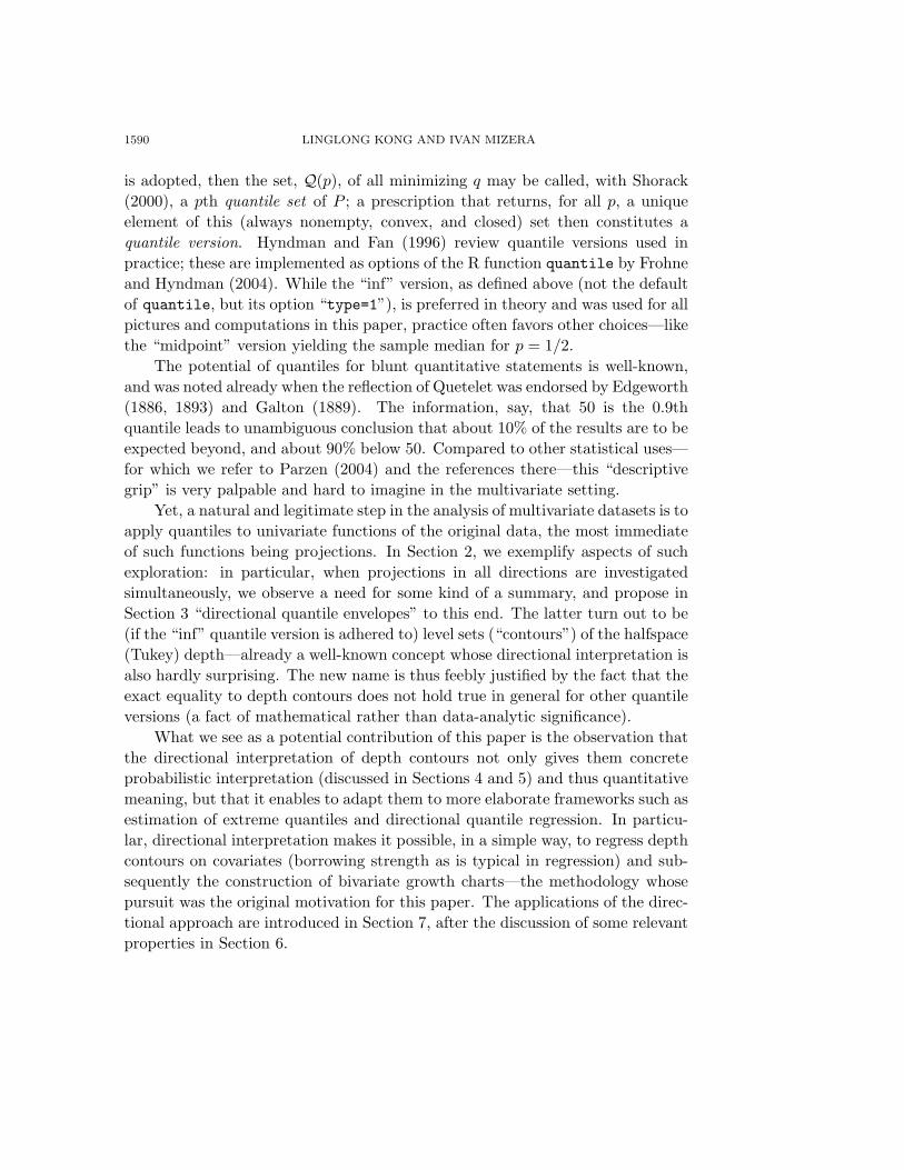
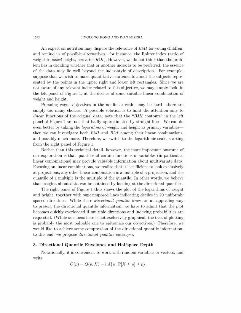
Figure 1. Left panel: multivariate data typically offer insights beyond themarginal view, often through the quantiles of univariate functions of primaryvariables. Right panel: the plot gets quickly overloaded if multiple directionsand indexing probabilities are requested.

2. Quantile Analysis of Projections, Illustrated on an Example

We illustrate the possible objectives of the analysis using quantiles in multi-variate setting with an example. The left panel of Figure 1 shows the scatterplotof the weight and height of 4291 Nepali children, aged between 3 and 60 months—the data constituting a part of the Nepal Nutrition Intervention Project-Sarlahi(NNIP-S, principal investigator Keith P. West, Jr., funded by the Agency of In-ternational Development). The horizontal and vertical lines show the deciles ofheight and weight, respectively, of the empirical distributions of the correspond-ing variables—indicating the simple conclusions that can be reached about thevariables. For instance, the points above the upper horizontal line correspond to10% of the subjects exceeding the others in height; similarly, the points right ofthe rightmost line correspond to 10% of those exceeding the others in weight.

It would be interesting to know what proportion of the data corresponds tothe upper right corner, but this information is not directly available (unless wecount the points manually). Regarding the subject labeled by 3, 110, for example,we can only say that its weight is somewhat higher than, but otherwise fairlyclose to the median; its height is about at the second decile, that is, exceedingabout 20% and exceeded by about 80% of its peers. Nevertheless, one couldargue that 3, 110 is in certain sense extremal, outstanding from the rest.

A possible way of substantiating this impression quantitatively is to invokeQuetelet’s body mass index (hereafter BMI ), defined as the ratio of weight tosquared height (in the metric system). The curved lines in the left panel ofFigure 1 show the deciles of the empirical distribution of the BMI. We can seethat in terms of BMI, the subject 3, 110 is indeed extreme, belonging to the groupof 10% of those with maximal BMI.


An expert on nutrition may dispute the relevance of BMI for young children,and remind us of possible alternatives—for instance, the Rohrer index (ratio ofweight to cubed height, hereafter ROI ). However, we do not think that the prob-lem lies in deciding whether that or another index is to be preferred; the essenceof the data may lie well beyond the index-style of description. For example,suppose that we wish to make quantitative statements about the subjects repre-sented by the points in the upper right and lower left rectangles. Since we arenot aware of any relevant index related to this objective, we may simply look, inthe left panel of Figure 1, at the deciles of some suitable linear combination ofweight and height.

Pursuing vague objectives in the nonlinear realm may be hard—there aresimply too many choices. A possible solution is to limit the attention only tolinear functions of the original data; note that the “BMI contours” in the leftpanel of Figure 1 are not that badly approximated by straight lines. We can doeven better by taking the logarithms of weight and height as primary variables—then we can investigate both BMI and ROI among their linear combinations,and possibly much more. Therefore, we switch to the logarithmic scale, startingfrom the right panel of Figure 1.

Rather than this technical detail, however, the more important outcome ofour exploration is that quantiles of certain functions of variables (in particular,linear combinations) may provide valuable information about multivariate data.Focusing on linear combinations, we realize that it is sufficient to look exclusivelyat projections; any other linear combination is a multiple of a projection, and thequantile of a multiple is the multiple of the quantile. In other words, we believethat insights about data can be obtained by looking at the directional quantiles.

The right panel of Figure 1 thus shows the plot of the logarithms of weightand height, together with superimposed lines indicating deciles in 20 uniformlyspaced directions. While these directional quantile lines are an appealing wayto present the directional quantile information, we have to admit that the plotbecomes quickly overloaded if multiple directions and indexing probabilities arerequested. (While our focus here is not exclusively graphical, the task of plottingis probably the most palpable one to epitomize our objectives.) Therefore, wewould like to achieve some compression of the directional quantile information;to this end, we propose directional quantile envelopes.

3. Directional Quantile Envelopes and Halfspace Depth

Notationally, it is convenient to work with random variables or vectors, andwrite

Q(p) = Q(p,X) = inf{u : P[X ≤ u] ≥ p},


despite that quantiles depend only on the distribution, P , of X. Hereafter, Xalways stands for a random vector with distribution P ; the apparent notationalconvention is to suppress the dependence on X when no confusion may arise. Wecall any vector with unit norm in Rd a normalized direction, and denote the setof all such vectors by Sd−1. Given a normalized direction s ∈ Sd−1 and 0 < p < 1,the pth directional quantile, in the direction s, is nothing but the pth quantile ofthe corresponding projection of the distribution of X,

Q(p, s) = Q(p, s,X) = Q(p, sTX).

A related notion is the pth directional quantile hyperplane, given by the equationsTx = Q(p, s). For d = 2, the hyperplanes amount to lines—which in our figuresindicate how directional quantiles divide the data.

The pth directional quantile in the direction s and the (1− p)-th directionalquantile in the direction −s are not necessarily equal—due to the inf conventionemployed in their definition. Nonetheless, they often coincide—for instance, it isnot possible to distinguish between any p-th and (1 − p)th directional quantilehyperplanes if for any projection of P , all quantile sets are singletons. A suffi-cient condition for this is that P has contiguous support : there is no intersectionof halfspaces with parallel boundaries that has nonempty interior but zero prob-ability P and divides the support of P to two parts. (Note that if the supportis not contiguous, it is not connected; however, it may be disconnected and stillcontiguous.) We believe that contiguous support is a fairly typical virtue of pop-ulation distributions, and consequently will limit most of our attention to p from(0, 1/2].

Contiguity of the support of X is also one of the things that implies con-tinuity, in s, of the directional quantiles. The following theorem is formulatedslightly more generally, to allow for alternative quantile versions and later asymp-totic considerations. Using the theorem with Xn = X shows that the directionalquantiles depend continuously on s for all empirical, and many population dis-tributions.

Theorem 1. If the support of X is bounded, then Q(p, s) is a continuous functionof s, for every p ∈ (0, 1). The same holds true when the support of X is contigu-ous; moreover, if a sequence of random vectors Xn converges almost surely to X,and sn → s, then Q(p, sn, Xn) converges to Q(p, s,X) in the Pompeiu-Hausdorffdistance, for every p ∈ (0, 1).

The terminology of “Pompeiu-Hausdorff” is that of Rockafellar and Wets(1998).

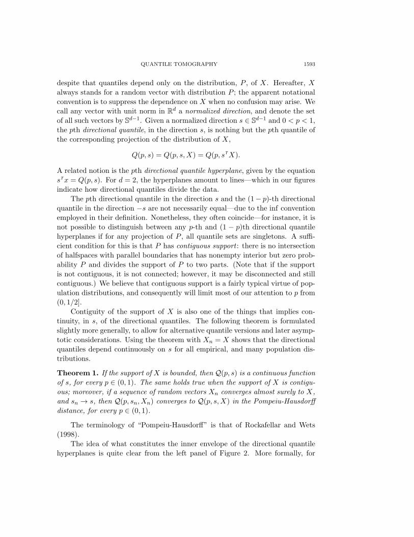
The idea of what constitutes the inner envelope of the directional quantilehyperplanes is quite clear from the left panel of Figure 2. More formally, for


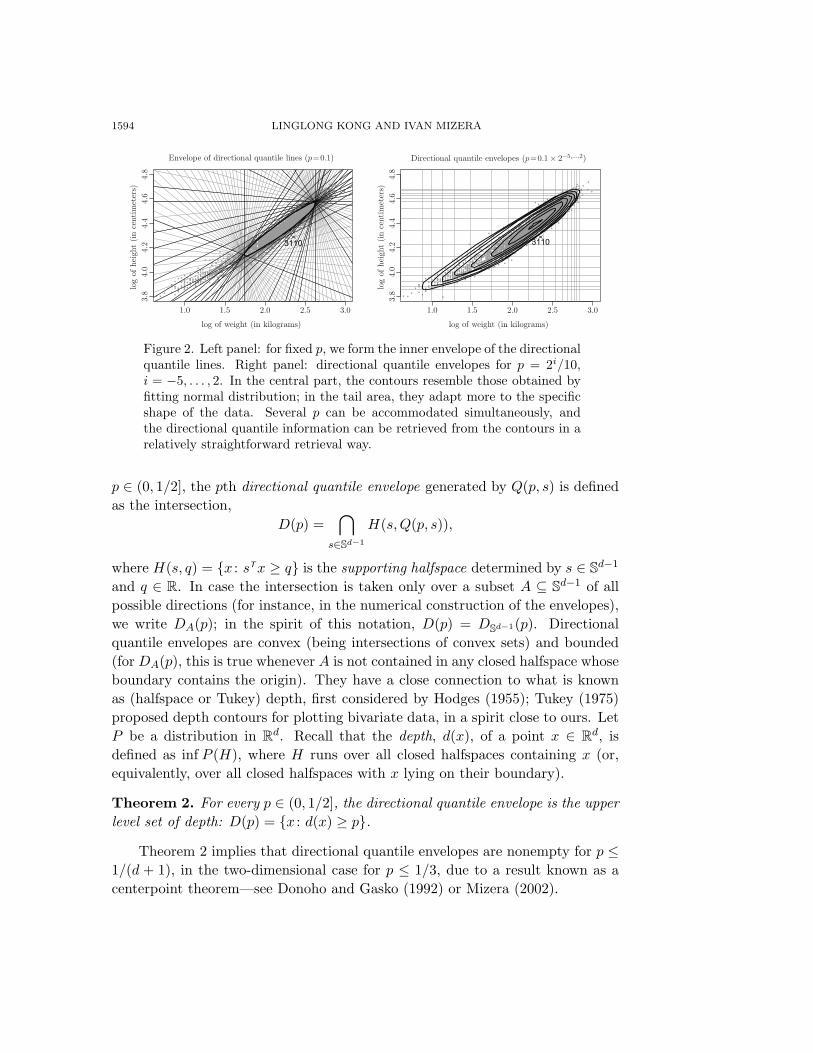
Figure 2. Left panel: for fixed p, we form the inner envelope of the directionalquantile lines. Right panel: directional quantile envelopes for p = 2i/10,i = −5, . . . , 2. In the central part, the contours resemble those obtained byfitting normal distribution; in the tail area, they adapt more to the specificshape of the data. Several p can be accommodated simultaneously, andthe directional quantile information can be retrieved from the contours in arelatively straightforward retrieval way.

p ∈ (0, 1/2], the pth directional quantile envelope generated by Q(p, s) is definedas the intersection,

D(p) ="

s∈Sd−1

H(s,Q(p, s)),

where H(s, q) = {x : sTx ≥ q} is the supporting halfspace determined by s ∈ Sd−1

and q ∈ R. In case the intersection is taken only over a subset A ⊆ Sd−1 of allpossible directions (for instance, in the numerical construction of the envelopes),we write DA(p); in the spirit of this notation, D(p) = DSd−1(p). Directionalquantile envelopes are convex (being intersections of convex sets) and bounded(for DA(p), this is true whenever A is not contained in any closed halfspace whoseboundary contains the origin). They have a close connection to what is knownas (halfspace or Tukey) depth, first considered by Hodges (1955); Tukey (1975)proposed depth contours for plotting bivariate data, in a spirit close to ours. LetP be a distribution in Rd. Recall that the depth, d(x), of a point x ∈ Rd, isdefined as inf P (H), where H runs over all closed halfspaces containing x (or,equivalently, over all closed halfspaces with x lying on their boundary).

Theorem 2. For every p ∈ (0, 1/2], the directional quantile envelope is the upperlevel set of depth: D(p) = {x : d(x) ≥ p}.

Theorem 2 implies that directional quantile envelopes are nonempty for p ≤1/(d + 1), in the two-dimensional case for p ≤ 1/3, due to a result known as acenterpoint theorem—see Donoho and Gasko (1992) or Mizera (2002).


We remark that Theorem 2 is rigorously true only for the “inf” version of thequantile definition. In practice, some other version may be preferred, for instance,to allow for constructing contours interpolating between various depth level sets.Most of our theorems hold true also for other versions, as can be seen in theAppendix; this fact gives some justification for calling what are essentially “depthcontours” by the new name “directional quantile envelopes”. All interpolatedversions of quantiles yield somewhat smaller envelopes; Rousseeuw and Ruts(1999) point out that this is also the case for the related notion of halfspacetrimmed contours of Masse and Theodorescu (1994). These subtle differencesvanish in regular situations—for instance, for absolutely continuous distributionswith positive densities.

4. Indexing, Illustrated on the Multivariate Normal Distribution

As can be seen on the right panel of Figure 2, suppressing the underlyingdirectional quantile lines (still shown in the left panel of Figure 2) allows foraccommodating several p simultaneously. In the central part, the contours haveelliptical shape, resembling the density contours of the multivariate normal dis-tribution. Indeed, Theorem 4 below implies that directional quantile envelopescoincide with the density contours for any elliptic distribution—in particular, forthe multivariate normal. In such a context, an intriguing question of practicalimportance is that of indexing: which particular contours of the fitted normaldistribution would correspond to which p?

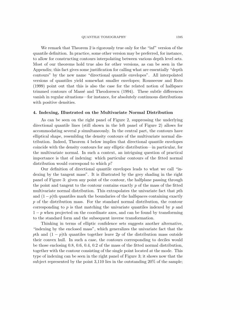
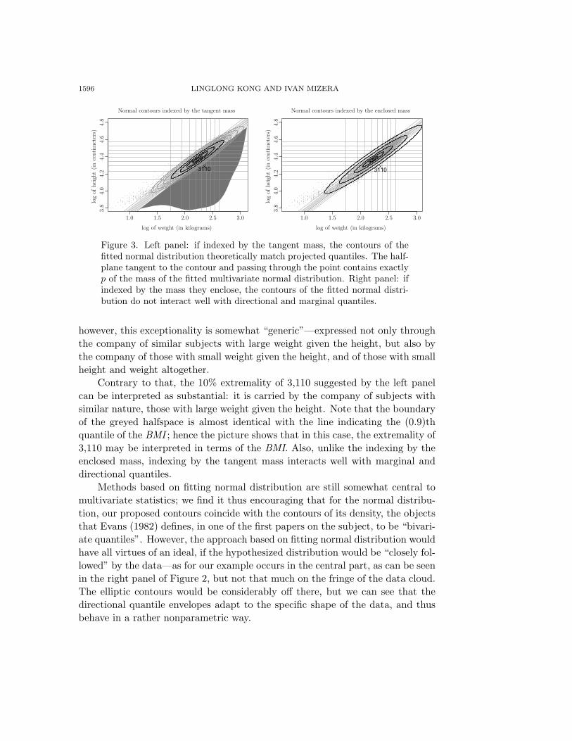
Our definition of directional quantile envelopes leads to what we call “in-dexing by the tangent mass”. It is illustrated by the grey shading in the rightpanel of Figure 3: given any point of the contour, the halfplane passing throughthe point and tangent to the contour contains exactly p of the mass of the fittedmultivariate normal distribution. This extrapolates the univariate fact that pthand (1− p)th quantiles mark the boundaries of the halfspaces containing exactlyp of the distribution mass. For the standard normal distribution, the contourcorresponding to p is that matching the univariate quantiles indexed by p and1− p when projected on the coordinate axes, and can be found by transformingto the standard form and the subsequent inverse transformation.

Thinking in terms of elliptic confidence sets suggests another alternative,“indexing by the enclosed mass”, which generalizes the univariate fact that thepth and (1 − p)th quantiles together leave 2p of the distribution mass outsidetheir convex hull. In such a case, the contours corresponding to deciles wouldbe those enclosing 0.8, 0.6, 0.4, 0.2 of the mass of the fitted normal distribution,together with the contour consisting of the single point located at the mode. Thistype of indexing can be seen in the right panel of Figure 3; it shows now that thesubject represented by the point 3,110 lies in the outstanding 20% of the sample;


Figure 3. Left panel: if indexed by the tangent mass, the contours of thefitted normal distribution theoretically match projected quantiles. The half-plane tangent to the contour and passing through the point contains exactlyp of the mass of the fitted multivariate normal distribution. Right panel: ifindexed by the mass they enclose, the contours of the fitted normal distri-bution do not interact well with directional and marginal quantiles.

however, this exceptionality is somewhat “generic”—expressed not only throughthe company of similar subjects with large weight given the height, but also bythe company of those with small weight given the height, and of those with smallheight and weight altogether.

Contrary to that, the 10% extremality of 3,110 suggested by the left panelcan be interpreted as substantial: it is carried by the company of subjects withsimilar nature, those with large weight given the height. Note that the boundaryof the greyed halfspace is almost identical with the line indicating the (0.9)thquantile of the BMI ; hence the picture shows that in this case, the extremality of3,110 may be interpreted in terms of the BMI. Also, unlike the indexing by theenclosed mass, indexing by the tangent mass interacts well with marginal anddirectional quantiles.

Methods based on fitting normal distribution are still somewhat central tomultivariate statistics; we find it thus encouraging that for the normal distribu-tion, our proposed contours coincide with the contours of its density, the objectsthat Evans (1982) defines, in one of the first papers on the subject, to be “bivari-ate quantiles”. However, the approach based on fitting normal distribution wouldhave all virtues of an ideal, if the hypothesized distribution would be “closely fol-lowed” by the data—as for our example occurs in the central part, as can be seenin the right panel of Figure 2, but not that much on the fringe of the data cloud.The elliptic contours would be considerably off there, but we can see that thedirectional quantile envelopes adapt to the specific shape of the data, and thusbehave in a rather nonparametric way.


5. Recovery of Directional Quantile Information

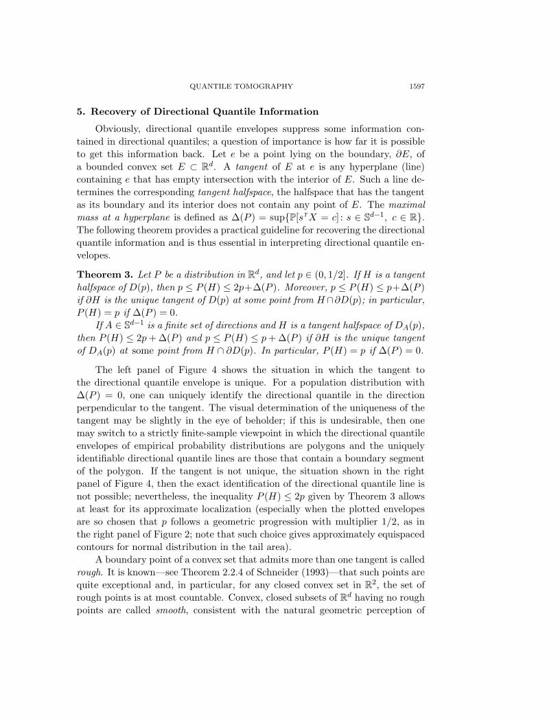
Obviously, directional quantile envelopes suppress some information con-tained in directional quantiles; a question of importance is how far it is possibleto get this information back. Let e be a point lying on the boundary, ∂E, ofa bounded convex set E ⊂ Rd. A tangent of E at e is any hyperplane (line)containing e that has empty intersection with the interior of E. Such a line de-termines the corresponding tangent halfspace, the halfspace that has the tangentas its boundary and its interior does not contain any point of E. The maximalmass at a hyperplane is defined as ∆(P ) = sup{P[sTX = c] : s ∈ Sd−1, c ∈ R}.The following theorem provides a practical guideline for recovering the directionalquantile information and is thus essential in interpreting directional quantile en-velopes.

Theorem 3. Let P be a distribution in Rd, and let p ∈ (0, 1/2]. If H is a tangenthalfspace of D(p), then p ≤ P (H) ≤ 2p+∆(P ). Moreover, p ≤ P (H) ≤ p+∆(P )if ∂H is the unique tangent of D(p) at some point from H∩∂D(p); in particular,P (H) = p if ∆(P ) = 0.

If A ∈ Sd−1 is a finite set of directions and H is a tangent halfspace of DA(p),then P (H) ≤ 2p+∆(P ) and p ≤ P (H) ≤ p+∆(P ) if ∂H is the unique tangentof DA(p) at some point from H ∩ ∂D(p). In particular, P (H) = p if ∆(P ) = 0.

The left panel of Figure 4 shows the situation in which the tangent tothe directional quantile envelope is unique. For a population distribution with∆(P ) = 0, one can uniquely identify the directional quantile in the directionperpendicular to the tangent. The visual determination of the uniqueness of thetangent may be slightly in the eye of beholder; if this is undesirable, then onemay switch to a strictly finite-sample viewpoint in which the directional quantileenvelopes of empirical probability distributions are polygons and the uniquelyidentifiable directional quantile lines are those that contain a boundary segmentof the polygon. If the tangent is not unique, the situation shown in the rightpanel of Figure 4, then the exact identification of the directional quantile line isnot possible; nevertheless, the inequality P (H) ≤ 2p given by Theorem 3 allowsat least for its approximate localization (especially when the plotted envelopesare so chosen that p follows a geometric progression with multiplier 1/2, as inthe right panel of Figure 2; note that such choice gives approximately equispacedcontours for normal distribution in the tail area).

A boundary point of a convex set that admits more than one tangent is calledrough. It is known—see Theorem 2.2.4 of Schneider (1993)—that such points arequite exceptional and, in particular, for any closed convex set in R2, the set ofrough points is at most countable. Convex, closed subsets of Rd having no roughpoints are called smooth, consistent with the natural geometric perception of


Figure 4. Left panel: if the tangent line to the pth directional quantileenvelope is unique, then the tangential halfspace is the pth directional quan-tile halfspace, in the given direction. Right panel: if the tangent line isnonunique, then this directional quantile halfspace lies between pth and(p/2)th directional quantile envelope.

the boundary in this case. If D(p) is smooth, then the collection of its tangenthalfspaces is in one-one correspondence with the collection of pth directionalquantile halfspaces, with the same boundaries, but in opposite directions.

Although the assumption of smoothness may sound optimistically mild, theexamples in Rousseeuw and Ruts (1999) show that distributions with depth con-tours having a few rough points are not that uncommon. However, it may beargued that all these examples have somewhat contrived flavor, especially whenthe support of the distribution is some regular geometric figure; it is not unlikelythat typical population distributions have smooth depth contours—but we werenot able to find a suitable formal condition reinforcing this belief, beyond thesomewhat restricted realm of elliptically-contoured distributions. Recall that adistribution is called elliptic if it can be transformed by an affine transformationto a circularly symmetric, rotationally-invariant distribution. The following the-orem, in particular, confirms the fact mentioned earlier: normal contours allowfor the retrieval of all directional quantile lines.

Theorem 4. The directional quantile envelopes of any elliptic distribution aresmooth.

Even if the tangent line at a boundary point of a directional quantile en-velope is nonunique, it does not necessarily mean that the information aboutcertain directional quantiles is lost. Although the directional quantile is notretrievable from the envelope directly, in a straightforward manner, it may bepossible to reconstruct it from the totality of all envelopes. Formally this meansthat the collection of directional quantile envelopes determines the distributionuniquely. Surprisingly, this plausible property has not yet been rigorously provedin full generality, positive answers have been established only for partial cases:


depth functions uniquely characterize empirical (Struyf and Rousseeuw (1999)),and more generally atomic (Koshevoy (2002)) distributions, and also absolutelycontinuous distributions with compact support (Koshevoy (2001)). A small stepin this direction is the following result of Kong and Zuo (2010) concerning dis-tributions with smooth depth contours.

Theorem 5. If the directional quantile envelopes D(p) of a probability dis-tribution P in Rd with contiguous support have smooth boundaries for everyp ∈ (0, 1/2), then there is no other probability distribution with the same di-rectional quantile envelopes.

6. Invariance, Approximation, and Estimation

Our considerations have been more probabilistic than statistical to this point;to advance the latter, the most straightforward way is to invoke the principlecalled “naıve statistics” by Hajek and Vorlıckova (1977), “analogy” by Gold-berger (1968) and Manski (1988), and “the plug-in principle” by Efron and Tib-shirani (1993): apply the general definition to empirical distributions.

From the general point of view, we are interested in the population quantileinformation, directional quantiles of some population distribution from which ourdata come, in some sampling manner,To facilitate theoretical analysis of typicalcases, it is often reasonable to posit some assumptions on this distribution; while amembership in a parametric family, or ellipticity may be considered too stringent,continuity assumptions are often acceptable. Our general strategy is to estimatethe result of the evaluation of a functional on the population distribution viathe application of the same functional to the empirical distribution supported bythe data. Specifically, we estimate, for fixed p, the directional quantiles Q(p, s)by Q(p, s), and then use these estimates to generate the estimated directionalquantile envelope.

Recall that an operator (we use this word to indicate that unlike a “func-tion”, an “operator” can be set-valued) assigning a point or a set T in Rd to acollection of datapoints xi ∈ Rd, is called affine equivariant, if its value is BT + bwhen evaluated from the datapoints Bxi + b, for any nonsingular matrix B andany b ∈ Rd. (If T is a set, then the transformations are performed elementwise.)By Theorem 2, the estimated and population directional quantile envelopes arethe level sets of depth applied to the empirical and population distributions, re-spectively; the properties of depth then imply their affine equivariance. Whendirectional quantiles are estimated by some other means, for instance as a re-sponse of a quantile regression, the affine equivariance of the resulting envelopesmay be not that clear. Nevertheless, the affine equivariance still holds undermild assumptions on the directional quantile estimators. Recall that an operator


that assigns a point, or set of points, T , in R, to a random variable X is calledtranslation equivariant, if its value for X+b coincides with T +b, and scale equiv-ariant, if its value for cX coincides with cT . It is a direct consequence of thedefinition that the directional quantile operator Q(p, ·) is translation and scaleequivariant for any 0 < p < 1 (and for the “inf” version; for every other version,the equivariance has to be checked individually—usually a straightforward task).

Theorem 6. Suppose that directional quantile estimators Q(p, s) are translationand scale equivariant for all s ∈ Sd−1 and fixed p. Then the directional quantileenvelope generated by these estimators is affine equivariant.

The next question we investigate is how quantile directional envelopes behavewhen not determined exactly, but only approximately. The numerical motiva-tion for this stems from the fact that in practice we are not able to take alldirections to construct the directional quantile envelope—what is constructed israther an approximate envelope DA(p), and we are interested in the quality ofthis approximation. Obviously, D(p) ⊆ DA(p); moreover, we believe that a de-cent collection, A, of directions that reasonably fill Sd−1 makes the approximationsatisfactory. While the experimental evidence does not contradict this belief—for the left panel of Figure 2 we used only 100 uniformly spaced directions, forthe right panel of Figure 2 we took 1009, and hardly any difference can be seenfor p = 0.1—some theoretical support would be desirable too. The statisticalmotivation for the investigation of the approximation effects comes from the factthat our directional quantiles are typically not the “true”, but “estimated” ones.If we believe that this estimation is consistent—we can show, in some custom-ary probabilistic framework, that estimates become more and more precise, say,with growing sample size—then we are again interested whether this consistentbehavior of individual directional quantiles translates into something analogousfor their envelopes.

Theorem 7. Suppose A1 ⊆ A2 ⊆ A3 ⊆ . . . is a sequence of closed sets with uniondense in a closed set A ⊆ Sd−1 that is not contained in any closed halfspace whoseboundary contains the origin. If, for every sequence sn ∈ An that converges to s ∈A, qn(sn) converges to q(s), then

#s∈An

H(s, qn(s)) converges to#

s∈AH(s, q(s))in the Pompeiu-Hausdorff distance—provided either the limit set is the closureof its interior, or is a singleton and the sets in the sequence are nonempty.

We illustrate the use of this theorem on two examples. In the first, we takeqn(s) = q(s) = Q(p, s); the successive approximations DA1(p) ⊇ DA2(p) ⊇ . . .then approachDA(p) in the Pompeiu-Hausdorff distance. Typically, An are finite,while A = Sd−1; the only requirements is that the directional quantiles Q(p, s)depend on s in a continuous way—for instance, P satisfies the assumptions of


Theorem 1. The second example leads to a proof of consistency, similar tothose given by He and Wang (1997), of Dn(p) to D(p), when the Dn(p) arise viaapplying the definition of directional quantile envelopes to empirical distributionsthat converge weakly almost surely to the sampled population distribution P ; therequired assumptions are those of Theorem 1, continuous or bounded support ofP , and the nondegeneracy of the limit D(p) (in general we cannot guarantee thatthe Dn(p) are nonempty). The Skorokhod representation then yields randomvariables Xn converging almost surely to random variables X, such that the lawsof Xn and X are the corresponding empirical distributions and P , respectively;Theorem 1 then implies the convergence assumption required by Theorem 7.

To obtain some idea of the magnitude of the approximation error, we proceedas follows (for simplicity, we limit our scope to the two-dimensional setting). Letd ∈ ∂D. The directions of all tangents of a convex set D at d generate a convexcone, TD(d). Let cD(d) be the maximal cosine between its two directions, thecosine of the maximal angle between two extremal normalized directions in TD(d),

c(d) = sup

$sT t

∥s∥∥t∥ : s, t ∈ TD(d)

%= sup

&sT t : s, t ∈ TD(d) ∩ Sd−1

'.

In fact, this cosine is the same as the maximal cosine of the directions in the nor-mal cone ND(d); see Rockafellar and Wets (1998), Chapter 6. We can see thatcD(d) ≤ 1, the equality holding if and only if TD(d) consists of single direction—when D has a unique tangent at d. Let κD = supd∈∂D

(2/(1 + c(d)), the re-

ciprocal of the cosine of the half of the maximal angle between directions in thetangent cone. Apparently, κD ≥ 1, the equality holding true for smooth D. Onthe other hand, κD can be +∞ for degenerate D, the sets with empty interior.

Theorem 8. Let A ⊆ S1 be a set of directions, and let q(s) and q(s) be two func-tions on A. If D =

#s∈AH(s, q(s)) and D =

#s∈AH(s, q(s)) are nondegenerate,

then κD and κD are finite and

d)D,D

*≤ max{κD,κD} sup

s∈A|q(s)− q(s)|,

where d denotes the Pompeiu-Hausdorff distance.

7. Directional Quantile Envelopes Beyond Simple Location Setting

So far, our methodology was demonstrated in the simple location setting,the situations in which there are no covariates and the estimation is performedvia the application of the quantile operators to empirical distributions. In thissection, we show how the directional definition can be used in more sophisticatedconstructions.


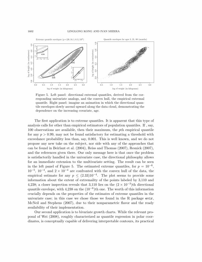
Figure 5. Left panel: directional extremal quantiles, derived from the cor-responding univariate analogs, and the convex hull, the empirical extremalquantile. Right panel: imagine an animation in which the directional quan-tile envelopes slowly ascend upward along the data cloud, demonstrating thedependence on the increasing covariate, age.

The first application is to extreme quantiles. It is apparent that this type ofanalysis calls for other than empirical estimators of population quantiles. If , say,100 observations are available, then their maximum, the pth empirical quantilefor any p > 0.99, may not be found satisfactory for estimating a threshold withexceedance probability less than, say, 0.001. This is well known, and we do notpropose any new take on the subject, nor side with any of the approaches thatcan be found in Beirlant et al. (2004), Reiss and Thomas (2007), Resnick (2007),and the references given there. Our only message here is that once the problemis satisfactorily handled in the univariate case, the directional philosophy allowsfor an immediate extension to the multivariate setting. The result can be seenin the left panel of Figure 5. The estimated extreme quantiles, for p = 10−6,10−5, 10−4, and 2 × 10−4 are confronted with the convex hull of the data, theempirical estimate for any p ≤ (2.33)10−4. The plot seems to provide someinformation about the extent of extremality of the points labeled by 3,110 and4,238; a closer inspection reveals that 3,110 lies on the (2 × 10−3)th directionalquantile envelope, with 4,238 on the (10−6)th one. The worth of this informationcrucially depends on the properties of the estimates of extreme quantiles in theunivariate case; in this case we chose those we found in the R package evir,McNeil and Stephens (2007), due to their nonparametric flavor and the readyavailability of their implementation.

Our second application is to bivariate growth charts. While the relevant pro-posal of Wei (2008), roughly characterized as quantile regression in polar coor-dinates, is conceptually capable of delivering interpretable contours, its practical


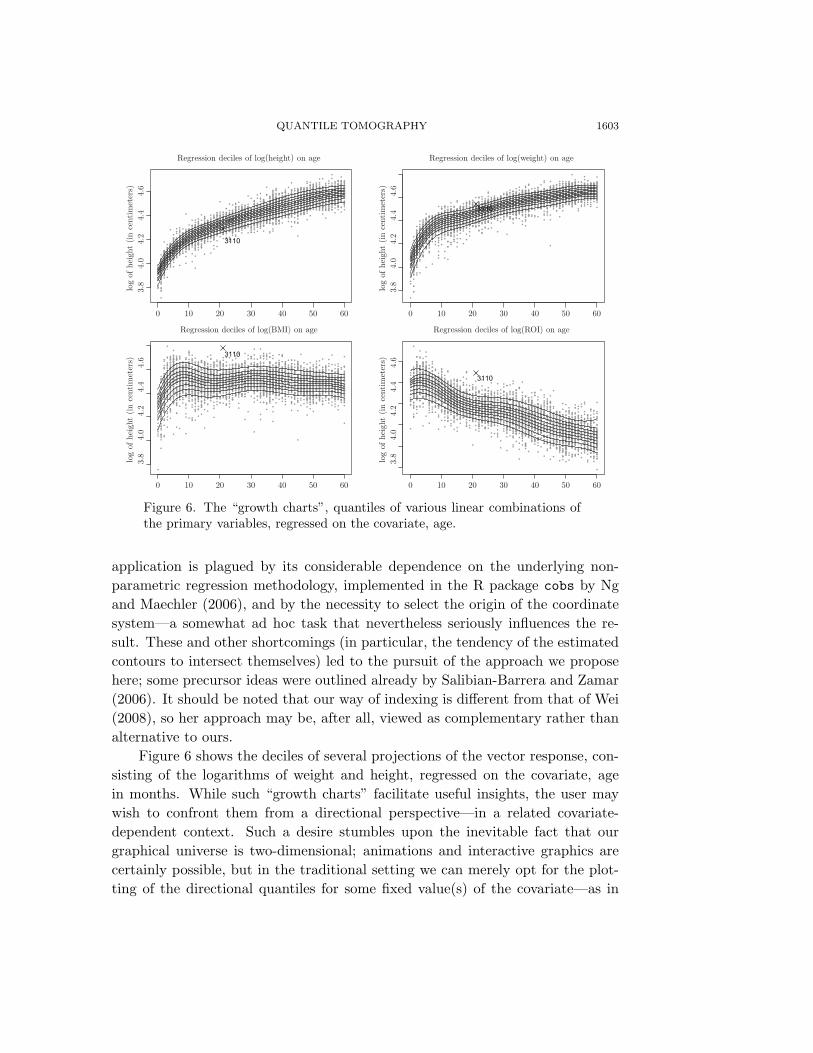
Figure 6. The “growth charts”, quantiles of various linear combinations ofthe primary variables, regressed on the covariate, age.

application is plagued by its considerable dependence on the underlying non-parametric regression methodology, implemented in the R package cobs by Ngand Maechler (2006), and by the necessity to select the origin of the coordinatesystem—a somewhat ad hoc task that nevertheless seriously influences the re-sult. These and other shortcomings (in particular, the tendency of the estimatedcontours to intersect themselves) led to the pursuit of the approach we proposehere; some precursor ideas were outlined already by Salibian-Barrera and Zamar(2006). It should be noted that our way of indexing is different from that of Wei(2008), so her approach may be, after all, viewed as complementary rather thanalternative to ours.

Figure 6 shows the deciles of several projections of the vector response, con-sisting of the logarithms of weight and height, regressed on the covariate, agein months. While such “growth charts” facilitate useful insights, the user maywish to confront them from a directional perspective—in a related covariate-dependent context. Such a desire stumbles upon the inevitable fact that ourgraphical universe is two-dimensional; animations and interactive graphics arecertainly possible, but in the traditional setting we can merely opt for the plot-ting of the directional quantiles for some fixed value(s) of the covariate—as in


the right panel of Figure 5 that shows the predicted envelopes for three valuesof age (selected so that the resulting envelopes do not overplot, rather than pur-suing any other objective). The highlighted datapoints represent the subjectsof the particular age. If we computed directional quantile envelopes from thesepoints separately, the resulting contours would be rougher, and would vary fromone value of age to another; the contours given in the right panel of Figure 5borrow strength from other ages, constructing quantile envelopes from a numberof quantile regressions, like those seen in Figure 6.

Once again, our focus is on how quantile regression blends into directionalquantile philosophy; from this perspective, our rendering of nonparametric quan-tile regression rather avoided than explored potential challenges, and we refer toKoenker (2005) and references there for the fine aspects of the methodology. Inview of Theorem 6, our main concern is whether the estimates are translation(regression) and scale equivariant, to yield affine equivariant envelopes—whichis true if the fits in Figure 6 and the right panel of Figure 5 are obtained viaregression splines, the methodology used by Wei et al. (2005) in their paperon growth charts. We used the automated knot selection furnished by the Rpackage splines, R Development Core Team (2007), and fitted quantile regres-sions by the R package quantreg, Koenker (2007). The smoothing parameterwas selected by eyeballing the plots included in Figure 6, and then adopting auniversal smoothing parameter for all directions in the right panel of Figure 5.We are aware of the possible shortcomings in certain engineering details—for in-stance that unlike in our situation, one can easily imagine data exhibiting moresignal-to-noise in certain directions than in others, the fact that would have tobe reflected in varying smoothing parameters; we hope to address these problemsin future research, as well as explore alternative possibilities for nonparametricquantile regression in the construction of growth charts.

8. Final Remarks

This paper is a shortened version of the preprint of Kong and Mizera (2008),dropping any mention of impasses like “quantile biplots” (so that they are notconfused with the concepts that we really champion); space considerations led usalso to omit the discussion of fine aspects of growth charts; finally, we do not dis-cuss any computational details, as those were rendered obsolete by developments—we hope to address computational aspects in a separate publication. We stillmaintain that our objective was not to propose any “multivariate quantile” gen-eralization of the univariate concept, akin to those reviewed in Serfling (2002).

We believe that directional quantile envelopes—which are, essentially, depthcontours—are a possible way to condense directional quantile information, theinformation carried by the quantiles of projections. In typical circumstances,


they allow for relatively faithful and straightforward retrieval of the directionalquantile information; the methodology offers straightforward probabilistic inter-pretations, and the estimated quantile envelopes are affine equivariant under mildequivariance assumptions on the estimators of directional quantiles. Most im-portantly, the directional interpretation can be adapted to elaborate frameworksrequiring more sophisticated quantile estimation methods than evaluating quan-tiles for empirical distributions, including estimation of extreme quantiles anddirectional quantile regression.

Acknowledgement

We are indebted to Ying Wei for turning our attention to multivariate growthcharts, as well as for many insights in Wei (2008), and to Roger Koenker for valu-able discussions. The directional approach to depth contours was pioneered inthe unpublished master thesis of Benoıt Laine, as reported by Koenker (2005)—in, however, quite significantly more complicated version fitting not directionalquantiles, but directional quantile regressions. Another important forerunner wasSalibian-Barrera and Zamar (2006). This research was supported by the Natu-ral Sciences and Engineering Research Council of Canada; some of the resultsoriginate from the doctoral dissertation of Kong (2009).

Appendix. Proofs

We define the pth directional quantile set to be the quantile set of the cor-responding projection:

Q(p, s) = Q(p, s,X) = Q(p, sTX).

Proof of Theorem 1. Since quantile sets are bounded intervals, it is sufficientto prove the convergence of their endpoints to inf Q(p, sTX) = inf{u : P[sTX ≤u] ≥ p} and supQ(p, sTX) = sup{u : P[sTX ≥ u] ≤ (1− p)}.

Suppose the support of X is bounded and let q = inf Q(p, sTX). We haveP[sTX ≤ q] ≥ p and P[sTX ≤ q − ε] < p. If the support of the distributionof X is bounded, we have ∥X∥ ≤ M almost surely; by the Schwarz inequality,|(s− sn)TX| ≤ M∥s− sn∥ and therefore

p ≤ P[sTX ≤ q] = P[sTnX ≤ q − (s− sn)

TX] ≤ P[sTnX ≤ q +M∥s− sn∥],

which means that inf Q(p, sTnX) ≤ q + M∥s − sn∥. In a similar fashion, weobtain that inf Q(p, sTnX) ≥ q − M∥s − sn∥ − ε, due to P[sT

nX ≤ q − M∥s −sn∥ − ε] ≤ P[sTX ≤ q − ε] < p. Letting ε → 0, we obtain q − M∥s − sn∥ ≤infQ(p, sT

nX) ≤ q + M∥s − sn∥, and therefore inf Q(p, sTnX) → infQ(p, sTX)


and thus also Q(p, sn, Xn) to Q(p, s,X). The convergence of supQ(p, sTnX) →

supQ(p, sTX) is proved analogously.If the support of the distribution of X is contiguous, then all directional

quantile sets in the limit are singletons. Pompeiu-Hausdorff convergence thenfollows from the “outer convergence” of quantile sets in the sense of Rockafellarand Wets (1998), see also Mizera and Volauf (2002): any limit point, x, of anysequence xn ∈ Q(p, sn, Xn) lies in Q(p, s,X). This can be easily seen in anelementary way, observing that xn ∈ Q(p, sn, Xn) entails

p ≤ lim supn→∞

P[sTnXn ≤ xn] ≤ P[sTX ≤ x],

1− p ≤ lim supn→∞

P[sTnXn ≥ xn] ≤ P[sTX ≥ x].

Since under the contiguous support assumption the quantiles are unique, thissecond part of the theorem holds true for every quantile version.Proof of Theorem 2. If y ∈ D(p), then y ∈ H(p, s) for every s ∈ Sd−1 andthus P ({x : sTx ≥ sTy}) ≥ p for all s ∈ Sd−1; therefore d(x) ≥ p. Conversely, ifd(y) ≥ p, then for every s ∈ Sd−1 we have P ({x : sTx ≥ sTy}) ≥ p. It followsthat sTy ≥ Q(p, s) and thus y ∈ H(p, s). Hence y ∈ D(p). As mentioned, thistheorem is true only for the “inf” definition, other quantile versions give smallerenvelopes.

Proof of Theorem 3. See Kong and Zuo (2010).

Proof of Theorem 4. By rotational invariance, the directional quantile en-velopes of any circularly symmetric distribution are circles; since elliptic distri-butions are those that can be transformed to the circular symmetric ones byan affine transformation, the theorem follows from their affine equivariance (andholds true for any quantile version).

Proof of Theorem 5. See Kong and Zuo (2010).

Proof of Theorem 6. Let B be a nonsingular matrix and b a vector. First,we verify the transformation rule for the supporting halfspace of the directionalquantile: for every s ∈ Sd−1 and every p ∈ (0, 1),

H(B∗s/∥B∗s∥, Q(p, s, BX + b)) = BH(s,Q(p, s,X)) + b, (A.1)

where B∗ = (B−1)T . If B is orthogonal, then B∗ = B, and if B is diagonal (moregenerally, symmetric), then B∗ = B−1. Indeed, the equation satisfied by x inBH(s, (Q, p, s,X)), sT

)B−1x

*≤ Q(p, s,X), is equivalent to ((B−1)Ts)Tx =

(B∗s)Tx ≤ Q(p, s,X). The norm of s is one, but not necessarily that of B∗s;therefore, we divide both sides by ∥B∗s∥, to write

(1/∥B∗s∥)(B∗s)Tx ≤ (1/∥B∗s∥)Q(p, s,X). (A.2)


By the scale equivariance of the quantile operator, and by the relationshipQ(p, s, AX) = Q(p,ATs,X) that follows directly from the definition, the right-hand side of (A.2) is Q(p, s,X/∥B∗s∥) = Q(p, s/∥B∗s∥, X) = Q(p,B∗s/∥B∗s∥,BX). Since the transformation BX + b is one-to-one, the transformed intersec-tion of halfspaces is the intersection of transformed halfspaces. Therefore, thetransformed directional quantile envelope is, by (A.1),

"

s∈Sd−1

(BH(p, s,X) + b) ="

s∈Sd−1

H(p,B∗s/∥B∗s∥, BX + b).

The proof is concluded by observing that s -→ B∗s/∥B∗s∥, where B∗ =(B−1)T , is a one-to-one transformation of Sd−1 onto itself—as can be seen by thedirect verification involving its inverse, t -→ BT t/∥BT t∥. The proof is the samefor any quantile version.

Proof of Theorem 7. To prove convergence with respect to Pompeiu-Hausdorffdistance, we exploit the following. The sequence

#s∈An

H(s, qn(s)), together withthe limit

#s∈AH(s, q(s)), is contained in a bounded set starting from some n,

since the sets An are approaching a dense set in A, and the latter is not containedin any halfspace whose boundary contains the origin; therefore this property isshared by An starting from some n, which means that

#s∈An

H(s, infk≥n qn(s))is the desired bounded set. For uniformly bounded sequences, the convergence inPompeiu-Hausdorff distance follows from the convergence in Painleve-Kuratowskisense; see Rockafellar and Wets (1998), 4.13. The latter means that a generalsequence of sets Kn converges to K if (i) every limit point of any sequencexn ∈ Kn lies in K, and (ii) every point from K is a limit of a sequence xn ∈ Kn;see also Mizera and Volauf (2002).

For sequences of closed sets with “solid” limits (sets that are closures oftheir interiors), the Painleve-Kuratowski convergence follows from the “rough”convergence, defined by Lucchetti, Salinetti, and Wets (1994) to require (i) and(ii)’ every limit point of every sequence yn ∈ (intKn)c is in (intK)c. The innerconvergence requirement of Painleve-Kuratowski definition is thus replaced bythe outer convergence for “closed complements”; see also Lucchetti, Torre, andWets (1993).

Suppose that y ∈ intK. Then y belongs to all but finitely many Kn; oth-erwise, there would be a subsequence ni such that y ∈ (intKni)

c and, by (ii)’,y ∈ (intK)c. Hence, every y from the relative interior of K is a limit of an(eventually constant) sequence yn ∈ Kn. To obtain (ii) for every x ∈ K, considera sequence yk of points from (nonempty) rintK such that yn → y; the desiredsequence xn is then obtained by a “diagonal selection”: for every yk, there is nk

such that yk ∈ Ki for every i ≥ k; set xn = yk for every nk ≤ n < nk+1.


Thus, it is sufficient to prove (i) and (ii)’. Suppose that x is a limit pointof a sequence xn ∈

#s∈An

H(s, qn(s)). Then there is a subsequence such thatsTnxn ≥ qn(sn) for every sn ∈ An; every s ∈ A is a limit of a sequence sn ∈ An,therefore the assumptions of the theorem imply that sTx ≥ q(s); hence x ∈#

s∈AH(s, q(s)). This proves (i) and the theorem for the singleton case, sincethen the Painleve-Kuratowski convergence is implied by (i) once the sets in thesequence are nonempty.

Suppose now that x is a limit point of a sequence xn∈(int#

s∈AnH(s, qn(s)))c,

that is, a limit of some subsequence of xn. Every such xn satisfies sTnxn ≤ qn(sn)

for some sn ∈ An. By the compactness of A, there is s ∈ A that is a limit of asubsequence of sn; passing to the limit along the appropriate subsequences, weobtain that sTx ≤ q(s), by the assumptions of the theorem. This means thatx ∈

)int

#s∈AH(s, q(s))

*c.

Proof of Theorem 8. As D and D are compact convex sets, we have d(D,D) =d(∂D, ∂D). Let ε = sups∈A |q(s) − q(s)|; we will show that for any x ∈ ∂D,d(x, ∂D) ≤ κDε. Let q(s) = q(s)− ε and D =

#s∈AH(s, q(s)).

For simplicity, we assume that D is also nondegenerate. We have that D ⊆D, and also D ⊆ D, the latter set being congruent to D. If κD(x) > 1, then x isa vertex of D. Since d(x, x) = κD(x)ε, where x is the corresponding congruentvertex in ∂D, it follows that d(x, ∂D) ≤ κDε. If κD(x) = 1, then by Theorem24.1 of Rockafellar (1996) there exists a sequence xn = x, xn ∈ ∂D, such thatxn → x and sn → s, κD(xn) = 1, where sn and s are the directions of the tangentlines passing through xn and x, respectively. There are two possibilities.

If there is N such that sn = s for any n > N , then there must be two points,denoted by y1 and y2, in ∂H(s, q(s))∩∂D such that κD(y1) > 1 and κD(y2) > 1.That is, y1 and y2 are two vertices of D and there is no other vertex between y1and y2 of D. Suppose that y1 and y2 are points congruent to them on D; theny1 and y2 are two vertices of D and there is no other vertex between y1 and y2of D as well. In other words, we have a trapezoid with vertices y1, y2, y1 andy2, and x lies on one of the bases. A simple geometric calculation then showsthe existence of a point, y, lying on the base constructed by y1 and y2, such thatd(x, y) ≤ max{κD(y1),κD(y2)}ε, that is, d(x, ∂D) ≤ κDε.

Suppose that there is an infinite subsequence of sn such that sn = s. Let∂D by xn and x be the congruent counterparts of xn and x, respectively; letsn and s be the corresponding directions. Let yn = ∂H(sn, q(sn)) ∩ ∂H(s, q(s))and yn = ∂H(sn, q(sn)) ∩ ∂H(s, q(s)). We have that yn → x, yn → x, andd(yn, yn) =

√2ε/

(1 + sTns. As d(yn, yn) → d(x, x) and

√2ε/

(1 + sTns → ε, we

have d(x, x) = ε, which means d(x, ∂D) ≤ κDε again.Taking into account that D ⊆ D, we obtain that d(x, ∂D) ≤ κDε for any

x ∈ ∂D. The theorem follows from this and the symmetric inequality, d(x, ∂D) ≤κDε for any x ∈ ∂D, which can established in an analogous way.


References

Beirlant, J., Goegebeur, Y., Teugels, J. and Segers, J. (2004). Statistics of Extremes: Theoryand Applications. Wiley, Chichester.

Donoho, D. L. and Gasko, M. (1992). Breakdown properties of location estimates based onhalfspace depth and projected outlyingness. Ann. Statist. 20, 1803-1827.

Edgeworth, F. Y. (1886). Problems in probabilities. London, Edinburgh, and Dublin Philosoph-ical Magazine and Journal of Science, 5th series 22, 371-384.

Edgeworth, F. Y. (1893). Exercises in the calculation of errors. London, Edinburgh, and DublinPhilosophical Magazine and Journal of Science, 5th series 36, 98-111.

Efron, B. and Tibshirani, R. J. (1993). An Introduction to Bootstrap. Chapman and Hall, NewYork.

Eubank, R. L. (1986). Quantiles. In Encyclopedia of Statistical Sciences, Volume 7 (Edited byS. Kotz, N. L. Johnson and C. B. Read), 424-432. Wiley, New York.

Evans, M. (1982). Confidence bands for bivariate quantiles. Commun. Statist.-Theor. Meth. 11,1465-1474.

Frohne, I. and Hyndman, R. J. (2004). quantile. A function in R starting from version 2.0.0,http://www.r-project.org.

Galton, F. (1888-1889). Co-relations and their measurement, chiefly from anthropometric data.Proc. Royal Soc. London 45, 135-145.

Goldberger, A. S. (1968). Topics in Regression Analysis. Macmillan, New York.

Hajek, J. and Vorlıckova, D. (1977). Mathematical Statistics. SPN, Praha. [in Czech].

He, X. and Wang, G. (1997). Convergence of depth contours for multivariate datasets. Ann.Statist. 25, 495-504.

Hodges, Jr, J. L. (1955). A bivariate sign test. Ann. Math. Statist. 26, 523-527.

Hyndman, R. J. and Fan, Y. (1996). Sample quantiles in statistical packages. Amer. Statist. 50,361-365.

Koenker, R. (2005). Quantile Regression. Cambridge University Press, Cambridge.

Koenker, R. (2007). quantreg: Quantile Regression. R package version 4.10, http://www.

r-project.org.

Kong, L. (2009). On multivariate quantile regression: Directional approach and application withgrowth charts. PhD thesis, University of Alberta.

Kong, L. and Mizera, I. (2008). Quantile tomography: using quantiles with multivariate data.ArXiv preprint arXiv:0805.0056v1.

Kong, L. and Zuo, Y. (2010). Smooth depth contours characterize underlying distribution. J.Multivariate Anal. 101, 2222-2226.

Koshevoy, G. A. (2001). Projections of lift zonoids, the Oja depth and Tukey depth. Preprint.

Koshevoy, G. A. (2002). The Tukey depth characterizes the atomic measure. J. MultivariateAnal. 83, 360-364.

Lucchetti, R., Salinetti, G. and Wets, R. J.-B. (1994). Uniform convergence of probabilitymeasures: topological criteria. J. Multivariate Anal. 51, 252-264.

Lucchetti, R., Torre, A. and Wets, R. J.-B. (1993). Uniform convergence of probability measures:topological criteria. Canad. Math. Bull. 36, 197-208.

Manski, C. F. (1988). Analog Estimation Methods in Econometrics. Chapman and Hall, NewYork.

http://www.r-project.org




Masse, J.-C. and Theodorescu, R. (1994). Halfplane trimming for bivariate distributions. J.Multivariate Anal. 48, 188-202.

McNeil, A. and Stephens, A. (2007). evir: Extreme Values in R. R package version 1.5, http://www.maths.lancs.ac.uk/~stephena/.

Mizera, I. (2002). On depth and deep points: A calculus. Ann. Statist. 30, 1681-1736.

Mizera, I. and Volauf, M. (2002). Continuity of halfspace depth contours and maximum depthestimators: diagnostics of depth-related methods. J. Multivariate Anal. 83, 365-388.

Ng, P. T. and Maechler, M. (2006). cobs: COBS - Constrained B-splines. R package version1.1-3.5, http://wiki.r-project.org/rwiki/doku.php?id=packages:cran:cobs.

Parzen, E. (2004). Quantile probability and statistical data modeling. Statist. Sci. 19, 652-662.

R Development Core Team (2007). R: A Language and Environment for Statistical Computing.R Foundation for Statistical Computing, Vienna. http://www.R-project.org.

Reiss, R.-D. and Thomas, M. (2007). Statistical Analysis of Extreme Values. Birkhauser Verlag,Basel.

Resnick, S. I. (2007). Heavy-Tail Phenomena: Probabilistic and Statistical Modeling. Springer,New York.

Rockafellar, R. T. (1996). Convex Analysis. Princeton University Press, Princeton.

Rockafellar, R. T. and Wets, R. J.-B. (1998). Variational analysis. Springer-Verlag, Berlin.

Rousseeuw, P. J. and Ruts, I. (1999). The depth function of a population distribution. Metrika49, 213-244.

Salibian-Barrera, M. and Zamar, R. (2006). Discussion of Conditional growth charts by Y. Weiand X. He. Ann. Statist. 34, 2113-2118.

Schneider, R. (1993). Convex bodies: The Brunn-Minkowski theory. Cambridge University Press,Cambridge.

Serfling, R. (2002). Quantile functions for multivariate analysis: approaches and applications.Statist. Neerlandica 56, 214-232.

Shorack, G. R. (2000). Probability for Statisticians. Springer-Verlag, New York.

Struyf, A. and Rousseeuw, P. J. (1999). Halfspace depth and regression depth characterize theempirical distribution. J. Multivariate Anal. 69, 135-153.

Tukey, J. W. (1975). Mathematics and the picturing of data. In Proceedings of the InternationalCongress of Mathematicians, Vol. 2, 523-531. Canad. Math. Congress, Quebec.

Wei, Y. (2008). An approach to multivariate covariate-dependent quantile contours with appli-cation to bivariate conditional growth charts. J. Amer. Statist. Assoc. 103, 397-409.

Wei, Y., Pere, A., Koenker, R. and He, X. (2005). Quantile regression methods for referencegrowth charts. Statist. in Medicine 25, 1369-1382.

Department of Mathematical and Statistical Sciences, University of Alberta, CAB 632, Edmon-ton, Alberta, T6G 2G1 Canada.

E-mail: [email protected]

Department of Mathematical and Statistical Sciences, University of Alberta, CAB 632, Edmon-ton, Alberta, T6G 2G1 Canada.

E-mail: [email protected]

(Received October 2010; accepted September 2011)

http://www.maths.lancs.ac.uk/~stephena/

http://www.maths.lancs.ac.uk/~stephena/

http://wiki.r-project.org/rwiki/doku.php?id=packages:cran:cobs

[email protected]

[email protected]

Documents

QUANTILE TOMOGRAPHY: USING QUANTILES WITH …mizera/Preprints/kongmize12.pdf · 1590 LINGLONG KONG AND IVAN MIZERA is adopted, then the set, Q(p), of all minimizing q may be called,