Embed Size (px)
Citation preview

Comptes Rendus
Mécanique
Salah Nissabouri, Mhammed El Allami and El Hassan Boutyour
Quantitative evaluation of semi-analytical finite element method formodeling Lamb waves in orthotropic platesVolume 348, issue 5 (2020), p. 335-350.
<https://doi.org/10.5802/crmeca.13>
© Académie des sciences, Paris and the authors, 2020.Some rights reserved.
This article is licensed under theCreative Commons Attribution 4.0 International License.http://creativecommons.org/licenses/by/4.0/
Les Comptes Rendus. Mécanique sont membres duCentre Mersenne pour l’édition scientifique ouverte
www.centre-mersenne.org
Comptes RendusMécanique2020, 348, n 5, p. 335-350https://doi.org/10.5802/crmeca.13
Quantitative evaluation of semi-analytical
finite element method for modeling Lamb
waves in orthotropic plates
Salah Nissabouri∗, a, Mhammed El Allamia, b and El Hassan Boutyourc
a Labo MISI, Department of Applied Physics, FST, Settat 26000, Morocco
b CRMEF, Settat, Morocco
c Labo MISI, FST, Settat 26000, Morocco
E-mails: [email protected] (S. Nissabouri), [email protected](M. El Allami), [email protected] (E. H. Boutyour)
Abstract. A semi-analytical finite element method algorithm was established to plot the dispersion curvesof isotropic aluminum and orthotropic plates. The curves obtained are compared with those plotted by theDISPERSE software and with previous experimental work. The results showed that the accuracy of the methoddepends on the number of elements for meshing. To ensure good precision and speed of the method, thenumber of elements per plate thickness must be optimized.
Keywords. SAFE, Dispersion curves, Isotropic, Orthotropic, Interpolation functions, Meshing.
Manuscript received 6th February 2020, revised 2nd April 2020 and 3rd May 2020, accepted 4th May 2020.
1. Introduction
Non-destructive testing (NDT) permits us to control the integrity of mechanical components inmany domains such as nuclear, medical, and aeronautic industries.
One of the most widely used ultrasonic methods is the control by Lamb waves. This kind ofwave is dispersive, and it is also sensitive to small defects. However, the presence of multiplemodes in a structure causes, in general, difficulties in terms of signal interpretation. For thisreason, it is important to choose an adequate frequency of Lamb mode excitation.
To choose an adequate frequency requires knowing precisely the dispersion curves of a testedstructure. These curves enable us to estimate the wavenumber, phase, and group velocities ofpropagating modes.
∗Corresponding author.
ISSN (electronic) : 1873-7234 https://comptes-rendus.academie-sciences.fr/mecanique/

336 Salah Nissabouri et al.
Figure 1. Dispersion curves plotted by the bisection method [1].
In previous research, the authors have discussed dispersion curves and their multiple applica-tions in NDT. They proposed several techniques to plot the dispersion curves. These methods in-clude the bisection method [1], the Newton–Raphson method [2], the transfer matrix method [3],the spectral method [4], and so on.
Moreover, the dispersion curves plotted by the iterative methods, even if they are very closeto analytical curves, present inaccuracy in determining the cutoff frequencies (Figure 1). For thisreason, we propose an alternative method, which allows a better estimation of the dispersioncurves.
The most robust methods of plotting dispersion curves for the case of isotropic and compositematerials are based on finite elements. However, they require significant storage capacities sincethey involve the meshing of the whole structure.
In this article, we use the semi-analytical finite element (SAFE) method. It is a method com-bining the semi-analytical and finite elements. The guided modes and their movements in thesection are calculated by the finite element method (FEM) and then supplemented by analyticaldisplacement in the propagation direction.
This method is optimal for predicting the propagating modes in a plate. This techniquerequires discretization only according to the thickness of the plate. Therefore, the calculationtimes are very short.
Moreover, this method adapts particularly well to the structures of complex geometries dis-cretized by finite elements. In addition, it allows us to characterize the properties of a wave prop-agating in an invariant section guide.
The SAFE method was first applied by Waas [5] for calculating the surface parameters of mul-tilayer soil. Afterward, it was used by many researchers for the study of Lamb wave propaga-tion in isotropic and composite structures. Ahmad et al. [6] applied the method for plottingthe dispersion curves of an aluminum plate and a composite-type structure [0/45/90/−45].Bartoli et al. [7] used the SAFE method to model the wave propagation of Lamb wavesin waveguides of an arbitrary section. The authors extended the use of the SAFE method
C. R. Mécanique, 2020, 348, n 5, 335-350

Salah Nissabouri et al. 337
Figure 2. Waveguide with a rectangular cross section.
to viscoelastic materials by considering damping. Takahiro et al. [8] simulated the propa-gation of Lamb waves in cylinders using the SAFE method. Takahiro et al. [9] calculateddispersion curves by the SAFE method. The curves obtained were compared with the ex-perimental curves calculated by two-dimensional (2D) fast Fourier transform. Mukdadi etal. [10] also studied the propagation of Lamb waves in multilayer composites. Predoi [11] pro-posed an extension of the SAFE method for periodic structures of infinite width. Recently,Wenbo et al. [12] have presented a formulation using the SAFE method and the perfectmatch layer technique for calculating pipeline dispersion curves immersed in a fluid. Xinget al. [13] proposed a defect localization method for rails and plotted rail dispersion curves bythe SAFE method. All the authors have studied the method, but no one has conducted a quanti-tative evaluation of dispersion curves plotted by the SAFE method.
The aims of this article are as follows:
• Establish an algorithm of the SAFE numerical method.• Calculate the dispersion curves of an isotropic plate and validate the results with the
DISPERSE software [14].• Calculate longitudinal and transverse displacements.• Calculate the dispersion curves of an orthotropic plate.
For this purpose, we start with a definition of the problem. Then we establish the equation ofmotion based on Hamilton’s principle. The relation obtained is discretized using interpolationfunctions. Subsequently, the relation is reformulated for the case of a plate in the form of aneigenvalue problem. Solving the equation makes it possible to find the propagating modesin isotropic and orthotropic plates. Finally, we evaluate the curves obtained by the DISPERSEsoftware and by previous experimental work. We observe that the accuracy of the methoddepends on the parameters that must be optimized.
2. Problem definition and equation of motion
2.1. Problem definition
We consider a waveguide with a rectangular cross section as presented in Figure 2.The wave propagates along the x-axis. Discretization is needed only in the cross section (2D
discretization). The wave propagates along the x-axis with a wavenumber k and an angularfrequency ω. The harmonic expression of the displacement is written in the form
u(x, y, z, t ) =U (y, z)exp−i(kx−ωt ). (1)
C. R. Mécanique, 2020, 348, n 5, 335-350

338 Salah Nissabouri et al.
2.2. Equation of motion
The equation for the eigenvalue problem is deduced from Hamilton’s relation [6]:
[K1 + ikK2 +k2K3 −ω2M ]U = 0. (2)
Here,
K1 =nel⋃e=1
k(e)1 ; K2 =
nel⋃e=1
k(e)2 ; K3 =
nel⋃e=1
k(e)3 ; M =
nel⋃e=1
m(e)
with
k(e)1 =
∫Ωe
[B T1 Ce B1]dΩe , (3)
k(e)2 = k(e)
21 −k(e)12 =
∫Ωe
[B T2 Ce B1]dΩe −
∫Ωe
[B T1 Ce B2]dΩe = (k(e)
21 )T −k(e)
12 , (4)
k(e)3 =
∫Ωe
[B T2 Ce B2]dΩe , (5)
m(e) =∫Ωe
[N Tρe N ]dΩe , (6)
where Ce is the elementary elastic matrix, ρe is the elementary mass density, nel is the number ofelements, and
B1 = Ly N,y +Lz N,z , (7)
B2 = Lx N . (8)
Here, N,y and N,z are the interpolation function derivatives with respect to variables y and z,respectively, and
Lx =
100000
000001
000010
; Ly =
000001
010000
000100
; Lz =
000010
000100
001000
.
N(y,z) is the matrix of interpolation functions expressed as
N (y, z) = N1 0
0 N1
0 0
0 N2
0 0N1 0
0 0N2 00 N2
· · ·Nn 0 00 Nn 00 0 Nn
.
3. SAFE formulation and solution of equation of motion for a plate
3.1. SAFE formulation
We consider the case of an infinite plate along the y-axis (Figure 3a). The displacement is thenindependent of y. Therefore, the plate can be modeled by one-dimensional (1D) elements. Theplane strain condition is considered here. Hence N,y = 0. Thus, Equations (7) and (8) becomeB1 = Lz N,z and B2 = Lx N , respectively.
The integrals given in (3)–(6) are computed numerically using the Gaussian quadraturemethod with three points. The integration limits need to be changed to −1 to 1. For this reason,the elements are discretized by isoparametric elements (Figure 3b).
The interpolation functions Ni with three nodes for the element are given by
N1(ξ) = ξ2 −ξ2
2; N2(ξ) = 1−ξ2; N3(ξ) = ξ2 +ξ2
2.
C. R. Mécanique, 2020, 348, n 5, 335-350
Salah Nissabouri et al. 339
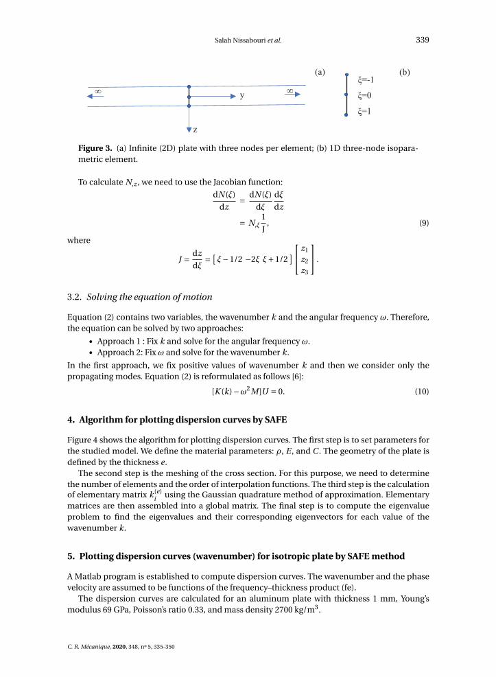
Figure 3. (a) Infinite (2D) plate with three nodes per element; (b) 1D three-node isopara-metric element.
To calculate N,z , we need to use the Jacobian function:
dN (ξ)
dz= dN (ξ)
dξ
dξ
dz
= N,ξ1
J, (9)
where
J = dz
dξ= [
ξ−1/2 −2ξ ξ+1/2] z1
z2
z3
.
3.2. Solving the equation of motion
Equation (2) contains two variables, the wavenumber k and the angular frequency ω. Therefore,the equation can be solved by two approaches:
• Approach 1 : Fix k and solve for the angular frequency ω.• Approach 2: Fix ω and solve for the wavenumber k.
In the first approach, we fix positive values of wavenumber k and then we consider only thepropagating modes. Equation (2) is reformulated as follows [6]:
[K (k)−ω2M ]U = 0. (10)
4. Algorithm for plotting dispersion curves by SAFE
Figure 4 shows the algorithm for plotting dispersion curves. The first step is to set parameters forthe studied model. We define the material parameters: ρ, E , and C . The geometry of the plate isdefined by the thickness e.
The second step is the meshing of the cross section. For this purpose, we need to determinethe number of elements and the order of interpolation functions. The third step is the calculationof elementary matrix k(e)
i using the Gaussian quadrature method of approximation. Elementarymatrices are then assembled into a global matrix. The final step is to compute the eigenvalueproblem to find the eigenvalues and their corresponding eigenvectors for each value of thewavenumber k.
5. Plotting dispersion curves (wavenumber) for isotropic plate by SAFE method
A Matlab program is established to compute dispersion curves. The wavenumber and the phasevelocity are assumed to be functions of the frequency–thickness product (fe).
The dispersion curves are calculated for an aluminum plate with thickness 1 mm, Young’smodulus 69 GPa, Poisson’s ratio 0.33, and mass density 2700 kg/m3.
C. R. Mécanique, 2020, 348, n 5, 335-350
340 Salah Nissabouri et al.
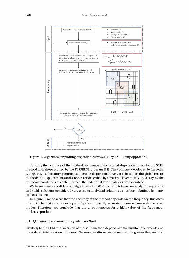
Figure 4. Algorithm for plotting dispersion curves ω (k) by SAFE using approach 1.
To verify the accuracy of the method, we compare the plotted dispersion curves by the SAFEmethod with those plotted by the DISPERSE program [14]. The software, developed by ImperialCollege NDT Laboratory, permits us to create dispersion curves. It is based on the global matrixmethod; the displacements and stresses are described by a material layer matrix. By satisfying theboundary conditions at each interface, the individual layer matrices are assembled.
We have chosen to validate our algorithm with DISPERSE as it is based on analytical equationsand yields solutions considered very close to analytical solutions as has been obtained by manyauthors [15–19].
In Figure 5, we observe that the accuracy of the method depends on the frequency–thicknessproduct. The first two modes A0 and S0 are sufficiently accurate in comparison with the othermodes. Therefore, we conclude that the error increases for a high value of the frequency–thickness product.
5.1. Quantitative evaluation of SAFE method
Similarly to the FEM, the precision of the SAFE method depends on the number of elements andthe order of interpolation functions. The more we discretize the section, the greater the precision
C. R. Mécanique, 2020, 348, n 5, 335-350

Salah Nissabouri et al. 341
Figure 5. Dispersion curves plotted by SAFE (continuous line) compared with dispersioncurves plotted by DISPERSE (dashed line).
Table 1. Relative errors for the calculation of mode A2 by SAFE as a function of n
Number of elements (n) Relative error4 1.46%5 0.8%6 0.46%
we obtain. In this case, as presented in Figure 5, we have meshed the section using two elementsin one dimension. We have used the quadratic interpolation function as we are interested in alow value of the frequency–thickness product.
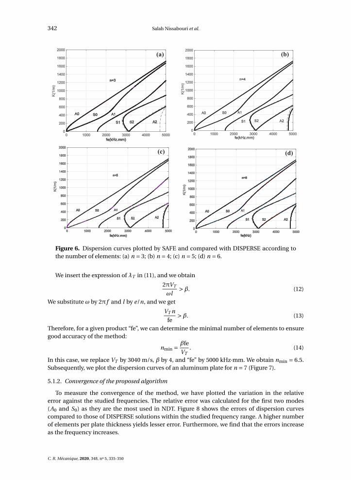
5.1.1. Effect of the number of elements on accuracy of SAFE method
Figure 6 shows that the accuracy of the method depends on the number of elements. Plotsfor meshing by three elements are shown in Figure 6a. The method permits us to calculate thefirst three modes A0, S0, and A1 with good precision. The modes S1 and S2 are calculated with anerror. To compute the A2 mode, we need to mesh the plate thickness by a number of elementsgreater than 4 (Table 1).
Table 1 shows that the error for the calculation of A2 by SAFE decreases for a number ofelements greater than 4.
Considering an isotropic plate with a thickness of 1 mm, if we are interested in frequencies upto 5000 kHz, then meshing by six elements is sufficient to compute the first six modes. However,if we are interested in frequencies greater than 5000 kHz, then we need to increase the number ofelements. This is proved by the author in [11]:
λT
l>β. (11)
Here, l is the length of the element, λT = 2πVT /ω is the wavelength of transverse waves propa-gating at velocity VT , and β= 4 in the case of quadratic interpolation functions [20].
C. R. Mécanique, 2020, 348, n 5, 335-350
342 Salah Nissabouri et al.
Figure 6. Dispersion curves plotted by SAFE and compared with DISPERSE according tothe number of elements: (a) n = 3; (b) n = 4; (c) n = 5; (d) n = 6.
We insert the expression of λT in (11), and we obtain
2πVT
ωl>β. (12)
We substitute ω by 2π f and l by e/n, and we get
VT n
fe>β. (13)
Therefore, for a given product “fe”, we can determine the minimal number of elements to ensuregood accuracy of the method:
nmin = βfe
VT. (14)
In this case, we replace VT by 3040 m/s, β by 4, and “fe” by 5000 kHz·mm. We obtain nmin = 6.5.Subsequently, we plot the dispersion curves of an aluminum plate for n = 7 (Figure 7).
5.1.2. Convergence of the proposed algorithm
To measure the convergence of the method, we have plotted the variation in the relativeerror against the studied frequencies. The relative error was calculated for the first two modes(A0 and S0) as they are the most used in NDT. Figure 8 shows the errors of dispersion curvescompared to those of DISPERSE solutions within the studied frequency range. A higher numberof elements per plate thickness yields lesser error. Furthermore, we find that the errors increaseas the frequency increases.
C. R. Mécanique, 2020, 348, n 5, 335-350
Salah Nissabouri et al. 343
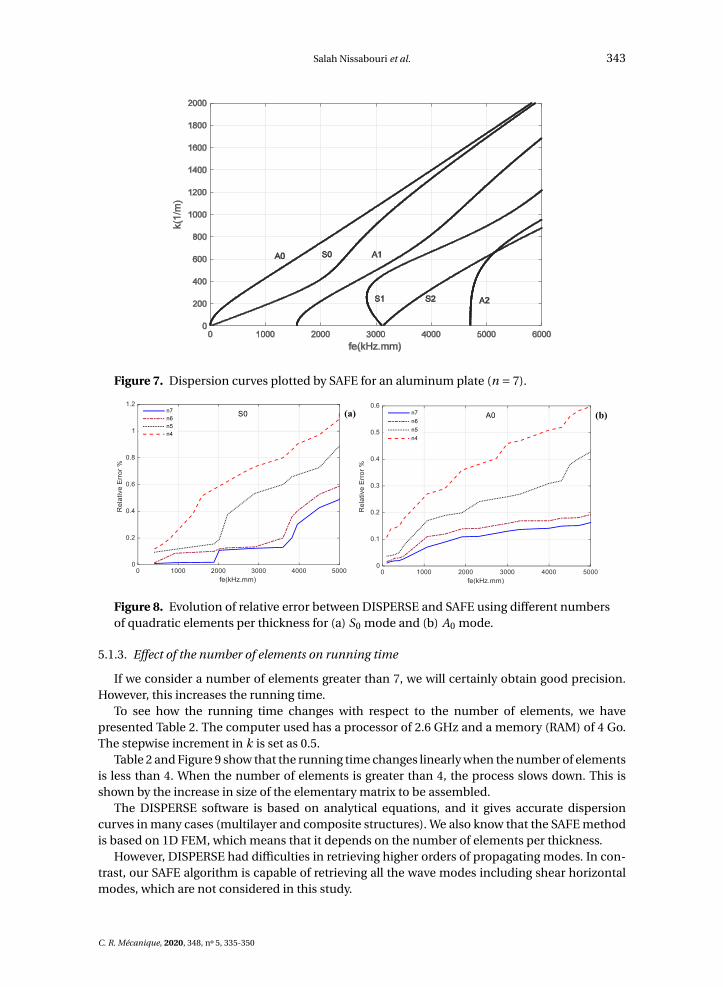
Figure 7. Dispersion curves plotted by SAFE for an aluminum plate (n = 7).
Figure 8. Evolution of relative error between DISPERSE and SAFE using different numbersof quadratic elements per thickness for (a) S0 mode and (b) A0 mode.
5.1.3. Effect of the number of elements on running time
If we consider a number of elements greater than 7, we will certainly obtain good precision.However, this increases the running time.
To see how the running time changes with respect to the number of elements, we havepresented Table 2. The computer used has a processor of 2.6 GHz and a memory (RAM) of 4 Go.The stepwise increment in k is set as 0.5.
Table 2 and Figure 9 show that the running time changes linearly when the number of elementsis less than 4. When the number of elements is greater than 4, the process slows down. This isshown by the increase in size of the elementary matrix to be assembled.
The DISPERSE software is based on analytical equations, and it gives accurate dispersioncurves in many cases (multilayer and composite structures). We also know that the SAFE methodis based on 1D FEM, which means that it depends on the number of elements per thickness.
However, DISPERSE had difficulties in retrieving higher orders of propagating modes. In con-trast, our SAFE algorithm is capable of retrieving all the wave modes including shear horizontalmodes, which are not considered in this study.
C. R. Mécanique, 2020, 348, n 5, 335-350

344 Salah Nissabouri et al.
Figure 9. Variation in running time with respect to the number of elements (n).
Table 2. Running time using SAFE as a function of the number of elements (n)
Number of elements Running time (s)1 20.282 43.043 64.774 89.0575 130.866 162.257 238.86
Figure 10 shows all the higher modes of dispersion curves plotted by SAFE and DISPERSE. Itillustrates that the SAFE method (even for n = 6 elements) permits us to compute more Lambmodes than does DISPERSE. Moreover, if we mesh the thickness of the studied plate with moreelements, the number of plotted modes increases. In addition, the DISPERSE software suffersfrom another limitation on materials and geometries with viscoelasticity, which is not the casefor the SAFE program [21].
5.2. Dispersion curves: phase velocity of an isotropic plate
The solution based on the SAFE method for the eigenvalue problem (10) helps in identifying theangular frequency ω for each increment in the wavenumber. Using the relation Vp =ω/k, we cancalculate the phase velocity for each value of the product “fe” (Figure 11).
5.3. Transverse and longitudinal displacements
The eigenvectors of (10) correspond to the longitudinal (ux ) and transverse (uz ) displacements.Figure 12 shows the displacement profiles through the plate thickness (1 mm) of an aluminum
plate at a frequency of 1000 kHz.
C. R. Mécanique, 2020, 348, n 5, 335-350

Salah Nissabouri et al. 345
Figure 10. Dispersion curves obtained by SAFE (continuous line) and by DISPERSE(dashed line) for an isotropic aluminum plate (n = 6).
Figure 11. Dispersion curves for an aluminum plate: phase velocity as a function of theproduct “fe” plotted by SAFE for n = 7.
6. Dispersion curves: phase velocity and wavenumber of an orthotropic plate
6.1. Wavenumber as a function of “fe”
We consider an orthotropic plate having the properties listed in Table 3. The dispersioncurves plotted by the iterative method of Newton–Raphson [2] were validated by experiments(Figure 13). We have chosen these curves as reference to validate the dispersion curves obtainedby SAFE.
C. R. Mécanique, 2020, 348, n 5, 335-350
346 Salah Nissabouri et al.
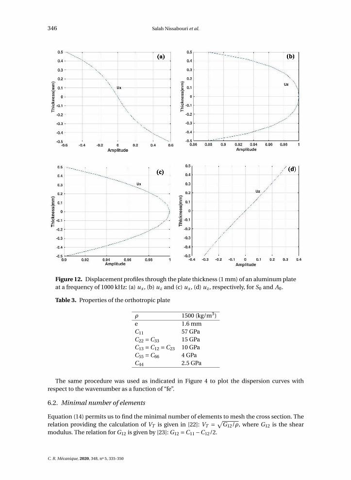
Figure 12. Displacement profiles through the plate thickness (1 mm) of an aluminum plateat a frequency of 1000 kHz: (a) ux , (b) uz and (c) ux , (d) uz , respectively, for S0 and A0.
Table 3. Properties of the orthotropic plate
ρ 1500 (kg/m3)e 1.6 mmC11 57 GPaC22 =C33 15 GPaC13 =C12 =C23 10 GPaC55 =C66 4 GPaC44 2.5 GPa
The same procedure was used as indicated in Figure 4 to plot the dispersion curves withrespect to the wavenumber as a function of “fe”.
6.2. Minimal number of elements
Equation (14) permits us to find the minimal number of elements to mesh the cross section. Therelation providing the calculation of VT is given in [22]: VT = √
G12/ρ, where G12 is the shearmodulus. The relation for G12 is given by [23]: G12 =C11 −C12/2.
C. R. Mécanique, 2020, 348, n 5, 335-350
Salah Nissabouri et al. 347
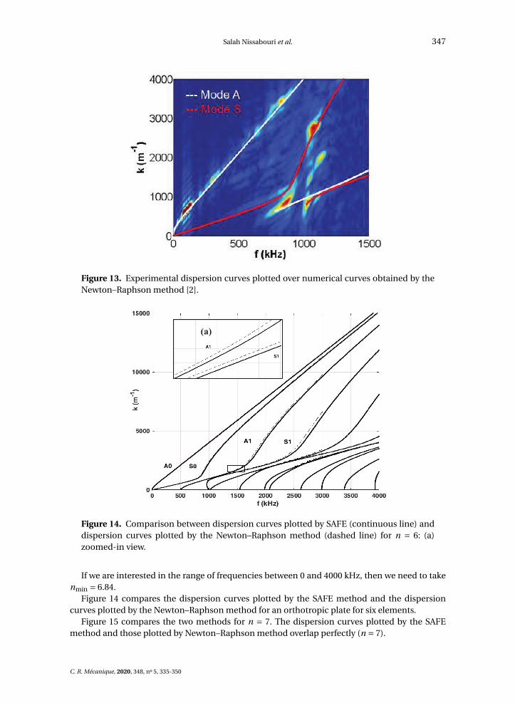
Figure 13. Experimental dispersion curves plotted over numerical curves obtained by theNewton–Raphson method [2].
Figure 14. Comparison between dispersion curves plotted by SAFE (continuous line) anddispersion curves plotted by the Newton–Raphson method (dashed line) for n = 6: (a)zoomed-in view.
If we are interested in the range of frequencies between 0 and 4000 kHz, then we need to takenmin = 6.84.
Figure 14 compares the dispersion curves plotted by the SAFE method and the dispersioncurves plotted by the Newton–Raphson method for an orthotropic plate for six elements.
Figure 15 compares the two methods for n = 7. The dispersion curves plotted by the SAFEmethod and those plotted by Newton–Raphson method overlap perfectly (n = 7).
C. R. Mécanique, 2020, 348, n 5, 335-350
348 Salah Nissabouri et al.
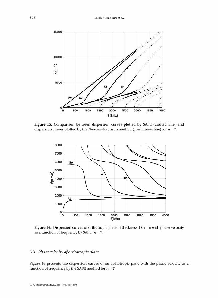
Figure 15. Comparison between dispersion curves plotted by SAFE (dashed line) anddispersion curves plotted by the Newton–Raphson method (continuous line) for n = 7.
Figure 16. Dispersion curves of orthotropic plate of thickness 1.6 mm with phase velocityas a function of frequency by SAFE (n = 7).
6.3. Phase velocity of orthotropic plate
Figure 16 presents the dispersion curves of an orthotropic plate with the phase velocity as afunction of frequency by the SAFE method for n = 7.
C. R. Mécanique, 2020, 348, n 5, 335-350
Salah Nissabouri et al. 349
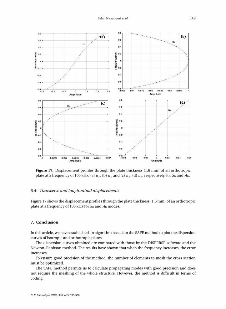
Figure 17. Displacement profiles through the plate thickness (1.6 mm) of an orthotropicplate at a frequency of 100 kHz: (a) ux , (b) uz and (c) ux , (d) uz , respectively, for S0 and A0.
6.4. Transverse and longitudinal displacements
Figure 17 shows the displacement profiles through the plate thickness (1.6 mm) of an orthotropicplate at a frequency of 100 kHz for S0 and A0 modes.
7. Conclusion
In this article, we have established an algorithm based on the SAFE method to plot the dispersioncurves of isotropic and orthotropic plates.
The dispersion curves obtained are compared with those by the DISPERSE software and theNewton–Raphson method. The results have shown that when the frequency increases, the errorincreases.
To ensure good precision of the method, the number of elements to mesh the cross sectionmust be optimized.
The SAFE method permits us to calculate propagating modes with good precision and doesnot require the meshing of the whole structure. However, the method is difficult in terms ofcoding.
C. R. Mécanique, 2020, 348, n 5, 335-350

350 Salah Nissabouri et al.
Acknowledgment
The authors would like to express their gratitude to Elhadji Barra Ndiaye, PhD, for his help.
References
[1] S. Nissabouri, M. El Allami, M. Bakhcha, “Lamb waves propagation plotting the dispersion curves”, in Conference:ICCWCS16Volume: PROCEEDINGSISSN, Morocco, 2016, p. 153-156.
[2] E. B. Ndiaye, H. Duflo, “Non destructive testing of sandwich composites: adhesion defects evaluation; experimentaland finite element method simulation comparison”, in Acoustics 2012 Nantes, Nantes, France, 2012, p. 2659-2664.
[3] A. Nayfeh, “The general problem of elastic wave propagation in multilayered anisotropic media”, J. Acoust. Soc. Am.(1991), p. 1521-1531.
[4] B. Sinha, H. P. Valero, F. Karpfinger, A. Bakulin, B. Gurevich, “Spectral-method algorithm for modeling dispersion ofacoustic modes in elastic cylindrical structures”, Geophysics 75 (2010), p. H19-H27.
[5] G. Waas, “Analysis report for footing vibrations through layered media”, PhD Thesis, University of California, 1972.[6] Z. A. B. Ahmad, J. M. Vivar-Perez, U. Gabbert, “Semi-analytical finite element method for modeling of lamb wave
propagation”, CEAS Aeronaut. J. 4 (2013), p. 21-33.[7] I. Bartoli, M. Alessandro, L. Francesco, V. Erasmo, “Modeling wave propagation in damped waveguides of arbitrary
cross-section”, J. Sound Vibrat. 295 (2006), p. 685-707.[8] H. Takahiro, K. Koichiro, S. Zongqi, L. Joseph, “Analysis of flexural mode focusing by a semi analytical finite element
method”, J. Acoust. Soc. Am. 113 (2003), p. 1241-1248.[9] H. Takahiro, S. Won-Joon, L. Joseph Rose, “Guided wave dispersion curves for a bar with an arbitrary cross-section,
a rod and rail example”, Ultrasonics 41 (2003), p. 175-183.[10] M. Osama, D. S. Mukdadi, “Transient ultrasonic guided waves in layered plates with rectangular cross section”,
J. Appl. Phys. 93 (2003), p. 9360-9363.[11] P. Mihai Valentin, “Guided waves dispersion equations for orthotropic multilayered pipes solved using standard
finite elements code”, Ultrasonics 54 (2014), p. 1825-1831.[12] D. Wenbo, K. Ray, “Guided wave propagation in buried and immersed fluid-filled pipes: Application of the semi
analytic finite element method”, Comput. Struct. 212 (2019), p. 236-247.[13] B. Xing, Y. Zujun, X. Xining, Z. Liqiang, S. Hongmei, “Research on a rail defect location method based on a single
mode extraction algorithm”, Appl. Sci. 9 (2019), p. 1-16.[14] B. Pavlakovic, M. Lowe, D. Alleyne, P. Cawley, “Disperse: A general purpose program for creating dispersion curves”,
in Review of Progress in Quantitative NDE, Springer, Boston, MA, 2013, p. 185-192.[15] R. Sanderson, “A closed form solution method for rapid calculation of guided wave dispersion curves for pipes”,
Wave Motion 53 (2015), p. 40-50.[16] L. Draudviliene, R. Raišutis, E. Žukauskas, A. Jankauskas, “Validation of dispersion curve reconstruction techniques
for the A0 and S0 modes of lamb waves”, Inti J. Struct. Stability Dyn. 14 (2014), p. 1-11.[17] B. Hernandez Crespo, C. R. P. Courtney, B. Engineer, “Calculation of guided wave dispersion characteristics using a
three-transducer measurement system”, Appl. Sci. 8 (2018), p. 1253.[18] B. Hernandez, B. Engineer, C. R. P. Courtney, “Empirical technique for dispersion curve creation for guided wave
applications”, in Conference: 8th European Workshop on Structural Health Monitoring, EWSHM, Spain, 2016.[19] S. Soua, S. Chan, T.-H. Gan, “Modelling of long range ultrasonic waves in complex structures”, in BINDT Annual
Conference, UK, 2008.[20] M. Jose, A. R. Galan, “Numerical simulation of Lamb wave scattering in semi-infinite plates”, Int. J. Numer. Meth.
Engng 53 (2002), p. 1145-1173.[21] F. Zhu, B. Wang, Z. Qian, E. Pan, I. E. Kuznetsova, “Accurate characterization of 3D dispersion curves and mode
shapes of waves propagating in generally anisotropic viscoelastic/elastic plates”, Intl J. Solids Struct. 150 (2018),p. 52-65.
[22] F. G. Lei Wang, “Yuan, Group velocity and characteristic wave curves of Lamb waves in composites: Modeling andexperiments”, Composit. Sci. Technol. 67 (2007), p. 1370-1384.
[23] K. A. Kaw, Mechanics of Composite Materials, 2nd ed., CRC Press, 2006.
C. R. Mécanique, 2020, 348, n 5, 335-350