Quantitative Methods in Economics Causality and treatment ...Treatment effects Sharp Regression Discontinuity Design I RDD is a fairly old idea (Thistlethwaite and Campbell, 1960)

Treatment effects

Quantitative Methods in EconomicsCausality and treatment effects

Maximilian Kasy

Harvard University, fall 2016

1 / 35

Treatment effects

8) The Regression Discontinuity Design

(cf. “Mostly Harmless Econometrics,” chapter 6)

2 / 35

Treatment effects

Sharp Regression Discontinuity DesignI Sometimes assignment for treatment D is determined based on

whether a unit exceeds some threshold c on a variable X (calledthe forcing variable or running variable):

Di = 1{Xi ≥ c} so Di =

{Di = 1 if Xi ≥ cDi = 0 if Xi < c

I Design arises often from administrative decisions, where theallocation of units to a program is partly limited for reasons ofresource constraints, and sharp rules rather than discretion byadministrators is used for allocation.

I Usually X is correlated with the outcomes Y so comparingtreated and untreated does not provide causal estimates.

I But we can use the discontinuity in E[Y |X ] at the cutoff valueX = c to estimate the effect of D on Y for units with X = c.

3 / 35

Treatment effects

Sharp Regression Discontinuity DesignI RDD is a fairly old idea (Thistlethwaite and Campbell, 1960) but

this design experienced a renaissance in recent years.I Thistlethwaite and Campbell (1960) study the effects of college

scholarships on later students’ achievements.I Scholarships are given on the basis of whether or not the

student’s test score is larger than some cutting value.I Treatment D is scholarshipI Forcing variable X is SAT score with cutoff cI Outcome Y is subsequent college gradesI Y0 denotes potential grades without the scholarshipI Y1 is potential grades with the scholarship

I Y1 and Y0 are correlated with X : on average, students with higherSAT scores obtain higher college grades.

I However, if E[Y1|X ] and E[Y0|X ] are continuous functions of X atX = c, then we can attribute any discontinuity in E[Y |X ] at X = cto the effect of the treatment.

4 / 35

Treatment effects

Sharp RDD: Graphical Interpretation

-

6

��

��

��

��

p p p p p p p p p p p p p p p p p p p p p p p pp p p p p p p p p p p

p p p p p p p p p p p p p p p pp p p p p p p p p p p p

c X

Y

(D = 1)(D = 0)

E[Y |X ,D]

E[Y0|X ]

E[Y1|X ]

6

?

E[Y1−Y0|X =c]

5 / 35

Treatment effects

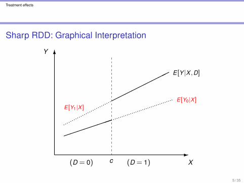
Sharp RDD: Graphical Interpretation

-

6

��

��

��

��



c X

Y

(D = 1)(D = 0)

E[Y |X ,D]

E[Y0|X ]

E[Y1|X ] 6

?

E[Y1−Y0|X =c]

5 / 35

Treatment effects

Sharp RDD: Identification

Identification Assumption

E[Y1|X ] and E[Y0|X ] are continuous at X = c

Identification Result

The treatment effect is identified at the threshold as:

E[Y1−Y0|X = c] = E[Y1|X = c]−E[Y0|X = c]

= limx↓c

E[Y |X = x]− limx↑c

E[Y |X = x]

6 / 35

Treatment effects

Continuity is a natural assumption but could be violated if:

I There are differences between the individuals who are just belowand above the cutoff that are not explained by the treatment (e.g.,the same cutoff is used to assign some other treatment)

I Subjects can manipulate the running variable in order to gainaccess to the treatment or to avoid it

7 / 35

Treatment effects

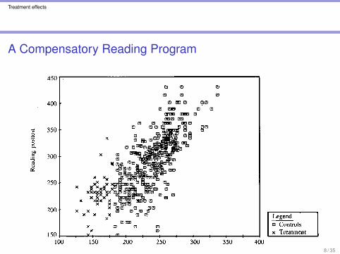
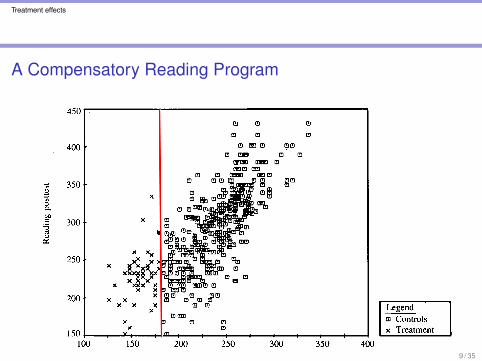
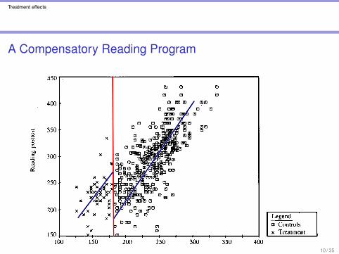
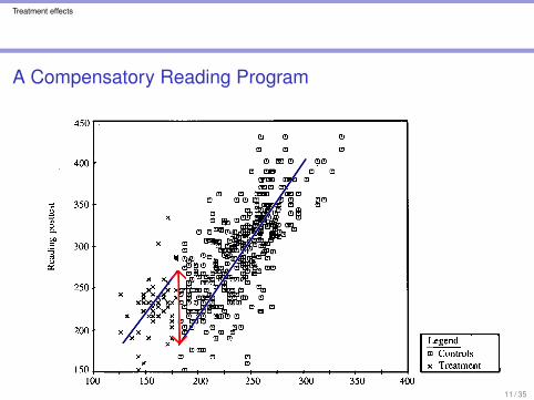
A Compensatory Reading Program

8 / 35

Treatment effects


9 / 35

Treatment effects


10 / 35

Treatment effects


11 / 35

Treatment effects

Sharp RDD Estimation: Linear Case

-

6

��

��

��

��



c X

Y

(D = 1)(D = 0)

E[Y |X ,D]

E[Y0|X ]

E[Y1|X ] 6

?

E[Y1−Y0|X =c]

12 / 35

Treatment effects

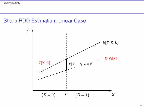
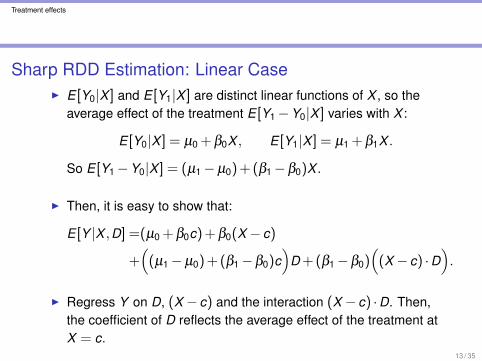
Sharp RDD Estimation: Linear CaseI E[Y0|X ] and E[Y1|X ] are distinct linear functions of X , so the

average effect of the treatment E[Y1−Y0|X ] varies with X :

E[Y0|X ] = µ0 +β0X , E[Y1|X ] = µ1 +β1X .

So E[Y1−Y0|X ] = (µ1−µ0)+(β1−β0)X .

I Then, it is easy to show that:

E[Y |X ,D] =(µ0 +β0c)+β0(X − c)

+((µ1−µ0)+(β1−β0)c

)D+(β1−β0)

((X − c) ·D

).

I Regress Y on D, (X − c) and the interaction (X − c) ·D. Then,the coefficient of D reflects the average effect of the treatment atX = c.

13 / 35

Treatment effects

Sharp RDD Estimation: Non-Linear Case

-

6

c X

Y

(D = 1)(D = 0)

E[Y |X ,D]

E[Y0|X ]

E[Y1|X ] 6

?

E[Y1−Y0|X =c]

14 / 35

Treatment effects

Sharp RDD Estimation: Non-Linear CaseI E[Y0|X ] and E[Y1|X ] are distinct non-linear functions of X and

the average effect of the treatment E[Y1−Y0|X ] varies with X .I Include quadratic and cubic terms in (X − c) and their

interactions with D in the equation.I The specification with quadratic terms is

E[Y |X ,D] =µ + γ1(X − c)+ γ2(X − c)2

+αD+δ1(X − c) ·D+δ2(X − c)2 ·D.

The specification with cubic terms is

E[Y |X ,D] =µ + γ1(X − c)+ γ2(X − c)2 + γ3(X − c)3 +αD

+δ1(X − c) ·D+δ2(X − c)2 ·D+δ3(X − c)3 ·D.

I In both cases α = E[Y1−Y0|X = c].15 / 35

Treatment effects

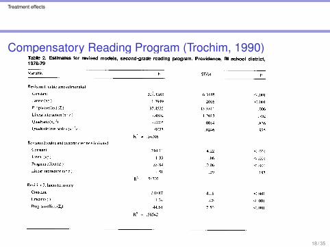
Compensatory Reading Program (Trochim, 1990)

I Evaluation of a compensatory reading program conducted amongsecond-graders in Providence (RI) in the late 70’s

I Comprehensive Test of Basic Skill was administered to studentsin 1978. Those who scored below certain cutoff (179) wereassigned to a compensatory reading program

I Y : a second test administered to the same students in 1979

I X : is the pre-test score

I D is assignment to the compensatory reading program

16 / 35

Treatment effects


17 / 35

Treatment effects


18 / 35

Treatment effects

Party Incumbency Advantage (Lee, 2008)

I Incumbent parties and candidates enjoy great electoral successin the U.S. and other countries

I Measuring incumbent advantage is difficult because “better”parties or candidates may be consistently favored by theelectorate

I Lee (2008) uses the Regression Discontinuity Design to studyparty incumbency advantage in the U.S.

I The data come from elections to the U.S. House ofRepresentatives (1946 to 1998)

19 / 35

Treatment effects

Party Incumbency Advantage (Lee, 2008)

20 / 35

Treatment effects

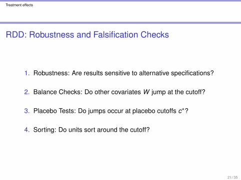
RDD: Robustness and Falsification Checks

1. Robustness: Are results sensitive to alternative specifications?

2. Balance Checks: Do other covariates W jump at the cutoff?

3. Placebo Tests: Do jumps occur at placebo cutoffs c??

4. Sorting: Do units sort around the cutoff?

21 / 35

Treatment effects

RDD: Robustness

6.1. SHARP RD 133

5

A. Linear E[Y0i| Xi]

.51

1.5

Out

com

e0

0 .2 .4 .6 .8 1X

B. Nonlinear E[Y0i| Xi]

.51

1.5

Out

com

e

[ 0i| i]

0O

0 .2 .4 .6 .8 1X

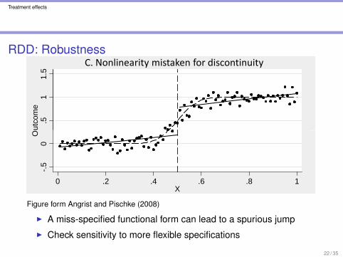
C Nonlinearity mistaken for discontinuity

.51

1.5

utco

me

C. Nonlinearity mistaken for discontinuity

-.50

O

0 .2 .4 .6 .8 1X

Figure 6.1.1: The sharp regression discontinuity design

Figure form Angrist and Pischke (2008)

I A miss-specified functional form can lead to a spurious jump

I Check sensitivity to more flexible specifications

22 / 35

Treatment effects

RDD: Balance Checks

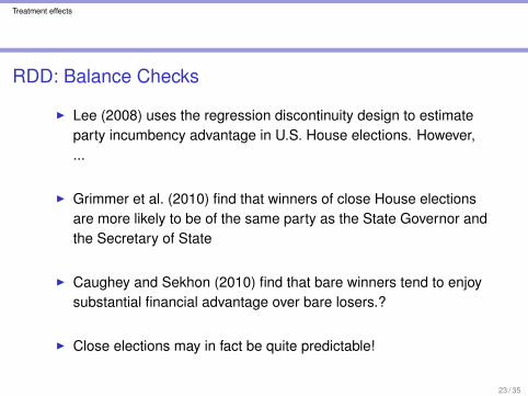
I Lee (2008) uses the regression discontinuity design to estimateparty incumbency advantage in U.S. House elections. However,...

I Grimmer et al. (2010) find that winners of close House electionsare more likely to be of the same party as the State Governor andthe Secretary of State

I Caughey and Sekhon (2010) find that bare winners tend to enjoysubstantial financial advantage over bare losers.?

I Close elections may in fact be quite predictable!

23 / 35

Treatment effects

RDD: Balance Checks (Grimmer et al., 2010)Figure 4: Gubernatorial and Electoral Administrative Control is Correlated with Winning CloseElections

0.0 0.2 0.4 0.6 0.8 1.0

0.0

0.2

0.4

0.6

0.8

Winners More Likely to Have Same Party as Governor

Share, Two Party Vote

Per

cent

Sam

e P

arty

Gov

erno

r

●

●

●

●

●

●

●●

●

●

●

●

●

●●

●

●

●

●

●

●

●

●●

●

●

●

●

●

●

●

●

●

●

●●

●

●

●

●

●

●

●

●

●

●●

●●

●

●●

●

●

●

●

●

●

●

●

●

●

●

●

●

●

●

●

●

●

●

●

●

●

●●

●

●

●

●

●

●

●

●

●●

●

●

●

●

●●

●

●

●

●

●

●

●

●●

●

●

●●●

●

●

●

●

●

●

●

●

●

●

●

●

●

●

●

●

●●

●●

●●

●

●

●

●●

●●

●

●

●●

●●

●

●

●●

●

●

●

●●

●●

●

●

●

●●

●●

●

●

●●

●

●

●

●

●

●●

●●

●

●●

●

●

●

●

●

●

●

●

●

●

●

●

●

●

●●

●

●●

●

●

●

●

0.0 0.2 0.4 0.6 0.8 1.0

0.0

0.2

0.4

0.6

0.8

Winners More Likely to Have Same Party as Election Adminstrator

Share, Two Party Vote

Per

cent

Sam

e P

arty

Ele

ctio

n A

dmin

istr

ator

This figure demonstrates that candidates who win very close elections are systematically more likely to belong tothe same party as the Governor and the election administrator (Secretary of State). The large gaps as the discontinuityin agreement betwene candidates and Governors (left-hand plot) and candidates and electoral administrators (right-hand plot) show that structural political advantages predict who win close elections. This is evidence that pre-electioncampaigning and post-election legal challenges are inducing differences in marginal elections.

6 percentage points more likely to belong to the same party as the Governor than candidates

who barely lost. Belonging to the same party as the election administrator also predicts who

wins extremely close elections. The right-hand plot of Figure 4 shows that candidates who win

extremely close elections are 5.5 percentage points more likely to belong to the same party than

candidates who barely lose. Bootstapped confidence intervals for both differences reveal that we

can confidently reject the null that the differences at the discontinuity are zero (p¡ 0.02).

The systematic political differences between candidates who win and lose very close elections

are robust to modeling choices and bandwidth selections. The left-hand plot in Figure 5 shows

that candidates who belong to the same party as the Governor are systematically more likely to

win marginal elections. We compare the proportion of candidates that win close elections in states

with a Governor who belongs to the same party to the proportion of candidates who win close

24

24 / 35

Treatment effects

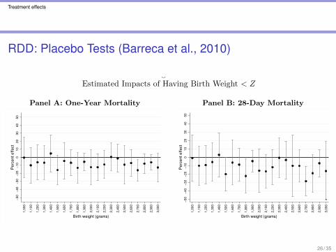
RDD: Placebo TestsI Almond et al. (2010) use a medical definition of “very low birth weight”<

1500 grams, to estimate the effect of additional medical care onnewborns

I They find that newborns just below the 1500 grams cutoff receiveadditional treatment and survive with higher probability than newbornsjust above the cutoff

I However, Barreca et al. (2010) find evidence of non-random rounding at100-gram multiples of birth weight

I Newborns of low socioeconomic status, who tend to be less healthy, aredisproportionately represented at 100-gram multiples (balance check)

I As a result, newborns with birth weights just below each 100-multiplehave more-favorable mortality outcomes than newborns with birthweights just above the cutoffs

25 / 35

Treatment effects

RDD: Placebo Tests (Barreca et al., 2010)

Figure 5Estimated Impacts of Having Birth Weight < Z

Panel A: One-Year Mortality Panel B: 28-Day Mortality

−50

−40

−30

−20

−10

010

20

30

40

50

Perc

ent effect

1,0

00

1,1

00

1,2

00

1,3

00

1,4

00

1,5

00

1,6

00

1,7

00

1,8

00

1,9

00

2,0

00

2,1

00

2,2

00

2,3

00

2,4

00

2,5

00

2,6

00

2,7

00

2,8

00

2,9

00

3,0

00

Birth weight (grams)

−50

−40

−30

−20

−10

010

20

30

40

50

Perc

ent effect

1,0

00

1,1

00

1,2

00

1,3

00

1,4

00

1,5

00

1,6

00

1,7

00

1,8

00

1,9

00

2,0

00

2,1

00

2,2

00

2,3

00

2,4

00

2,5

00

2,6

00

2,7

00

2,8

00

2,9

00

3,0

00

Birth weight (grams)

Note: Results are based on Vital Statistics Linked Birth and Infant Death Data,United States, 1983–2002 (not including 1992–1994). Following ADKW, esti-mates use a bandwidth of 85 grams and rectangular kernel weights, standarderrors are clustered at the gram-level, and all models include a linear trend inbirth weights that is flexible on either side of the cutoff.

30

26 / 35

Treatment effects

RDD: Sorting/Bunching

I Subjects or program administrators may invalidate the continuityassumption if they strategically manipulate X to be just above orbelow the cutoff

I This is a concern especially if the exact value of the cutoff isknown to the subjects in advance

I This type of behavior, if it exists, may create a discontinuity in thedistribution of X at the cutoff (i.e., “bunching” to the right or to theleft of the cutoff)

I A formal test is provided by McCrary (2008)

27 / 35

Treatment effects

RDD: Sorting/Bunching (Camacho and Conover, 2010)Example: Manipulation of a poverty index in Colombia. A poverty index isused to decide eligibility for social programs. The algorithm to create thepoverty index becomes public during the second half of 1997.

Figure 1: 1994-2003 Poverty Index Score Distribution

Note: Each figure corresponds to the interviews conducted in a given year, restricting the sample

to households living in strata levels below four. Using local linear regressions and an optimal

bandwidth algorithm we estimate the size of the discontinuity for each year as follows: 0.033

(1994); 0.080 (1995); 0.08 (1996); 0.024 (1997); 0.868***(1998); 1.209***(1999); 1.422***(2000);

1.683***(2001); 1.565***(2002); 1.547***(2003), where *** indicates significance at 1%.

28 / 35

Treatment effects

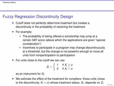
Fuzzy Regression Discontinuity DesignI Cutoff does not perfectly determine treatment but creates a

discontinuity in the probability of receiving the treatment

I For example:I The probability of being offered a scholarship may jump at a

certain SAT score (above which the applications are given “specialconsideration”)

I Incentives to participate in a program may change discontinuouslyat a threshold, but the change is not powerful enough to move allunits from nonparticipation to participation

I For units close to the cutoff we can use

Zi =

{1 if Xi ≥ c0 if Xi < c

as an instrument for Di .

I We estimate the effect of the treatment for compliers: those units (closeto the discontinuity, Xi ' c) whose treatment status, Di , depends on Zi .

29 / 35

Treatment effects

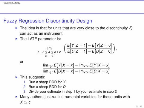
Fuzzy Regression Discontinuity DesignI The idea is that for units that are very close to the discontinuity Zi

can act as an instrumentI The LATE parameter is:

limc− ε ≤ X ≤ c+ ε

ε → 0

(E[Y |Z = 1]−E[Y |Z = 0]E[D|Z = 1]−E[D|Z = 0]

),

orlimx↓c E[Y |X = x]− limx↑c E[Y |X = x]limx↓c E[D|X = x]− limx↑c E[D|X = x]

I This suggests:1. Run a sharp RDD for Y2. Run a sharp RDD for D3. Divide your estimate in step 1 by your estimate in step 2

I Many authors just run instrumental variables for those units withX ' c

30 / 35

Treatment effects

Early Release Program (Marie, 2009)I Prison systems in many countries suffer from overcrowding and

high recidivism rates after release.

I Some countries use early discharge of prisoners on electronicmonitoring.

I Difficult to estimate impact of early release program on futurecriminal behavior: best behaved inmates are usually the ones tobe released early.

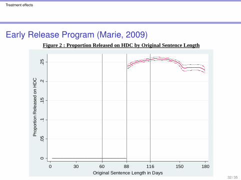
I Marie (2008) considers the Home Detention Curfew (HDC)program in England and Wales.

I This is a fuzzy RDD: Only offenders sentenced to more thanthree months (88 days) in prison are eligible for HDC, but not allof those are offered HDC.

31 / 35

Treatment effects

Early Release Program (Marie, 2009)

Figure 1: Distribution of Original Sentence Lengths in Days

05

7.5

1012

.52.

5P

erce

ntag

e R

elea

sed

0 88 180 365 730 1095 1460Original Sentence Length in Days

Non HDC Release HDC Release

Note: Line smoothed with 14 days local averages.

Figure 2 : Proportion Released on HDC by Original Sentence Length0

.05

.1.1

5.2

.25

Prop

ortio

n R

elea

sed

on H

DC


Note: Dotted lines show the confidence intervals. Line smoothed with 14 days local averages.32 / 35

Treatment effects

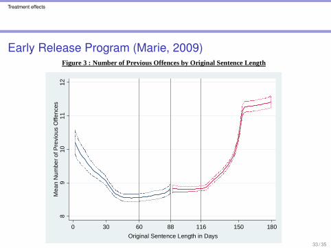
Early Release Program (Marie, 2009)Figure 3 : Number of Previous Offences by Original Sentence Length

89

1011

12M

ean

Num

ber o

f Pre

viou

s O

ffenc

es


Note: Dotted lines show the confidence intervals. Line smoothed with 14 days local averages.

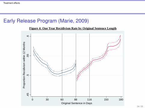
Figure 4: One Year Recidivism Rate by Original Sentence Length

.45

.5.5

5.6

Pro

porti

on R

ecid

ivis

m w

ithin

12

Mon

ths

0 30 60 88 116 150 180Original Sentence in Days


33 / 35

Treatment effects

Early Release Program (Marie, 2009)

Figure 3 : Number of Previous Offences by Original Sentence Length

89

1011

12M

ean

Num

ber o

f Pre

viou

s O

ffenc

es



Figure 4: One Year Recidivism Rate by Original Sentence Length.4

5.5

.55

.6P

ropo

rtion

Rec

idiv

ism

with

in 1

2 M

onth

s

0 30 60 88 116 150 180Original Sentence in Days

Note: Dotted lines show the confidence intervals. Line smoothed with 14 days local averages.34 / 35

Treatment effects

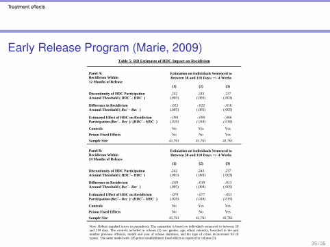
Early Release Program (Marie, 2009)Table 5: RD Estimates of HDC Impact on Recidivism

Panel A:Recidivism Within12 Months of Release

Estimation on Individuals Sentenced toBetween 58 and 118 Days: +/- 4 Weeks

(1) (2) (3)

Discontinuity of HDC ParticipationAround Threshold ( HDC+– HDC- )

.242(.003)

.243(.003)

.237(.003)

Difference in RecidivismAround Threshold ( Rec+– Rec- )

-.023(.005)

-.022(.005)

-.016(.005)

Estimated Effect of HDC on RecidivismParticipation (Rec+– Rec- )/ (HDC+– HDC- )

-.094(.020)

-.090(.018)

-.066(.018)

Controls No Yes YesPrison Fixed Effects No No Yes

Sample Size 41,761 41,761 41,761

Panel B:Recidivism Within24 Months of Release

Estimation on Individuals Sentenced toBetween 58 and 118 Days: +/- 4 Weeks

(1) (2) (3)

Discontinuity of HDC ParticipationAround Threshold ( HDC+– HDC- )

.242(.003)

.243(.003)

.237(.003)

Difference in RecidivismAround Threshold ( Rec+– Rec- )

-.019(.005)

-.019(.004)

-.013(.005)

Estimated Effect of HDC on RecidivismParticipation (Rec+– Rec- )/ (HDC+– HDC- )

-.079(.020)

-.077(.018)

-.053(.019)

Controls No Yes YesPrison Fixed Effects No No Yes

Sample Size 41,761 41,761 41,761

Note: Robust standard errors in parenthesis. The estimation is based on individuals sentenced to between 59and 118 days. The controls included in column (2) are: gender, age, ethnic minority, breached in the pastnumber previous offences, month and year of release dummies, and the type of crime incarcerated for (8types). The same model with 126 prison establishment fixed effects is reported in column (3).

35 / 35

Documents

Quantitative Methods in Economics Causality and treatment ...Treatment effects Sharp Regression Discontinuity Design I RDD is a fairly old idea (Thistlethwaite and Campbell, 1960)