Embed Size (px)
Citation preview

QUANTITATIVE TECHNIQUES FOR BUSINESS
(BBA4 C04)
STUDY MATERIAL
IV SEMESTER
BBA
(2019 Admission)
UNIVERSITY OF CALICUT
SCHOOL OF DISTANCE EDUCATION
CALICUT UNIVERSITY P.O
MALAPPURAM – 673 635, KERALA
19662
UNIVERSITY OF CALICUT
SCHOOL OF DISTANCE EDUCATION
BBA4C05 Quantitative Techniques for Business
Complementary Course – BBA 2019 Admission
Prepared by:
1. Dr.P Siddeeque
Assistant Professor
School of Distance Education,
University of Calicut
2. Sri. Vineethan T,
Assistant Professor, Department of Commerce,
Govt. College, Madappally
Scruitinized by:
Dr.Abbas Vattoli
Assistant Professor
Amal College of Advanced Studies
Nilambur

Module Contents Page
I Quantitative Techniques 2 – 11
2 Time Series and Index Number 12 – 32
3 Correlation and Regression Analysis 33 – 92
4 Probability 93 – 137
5 Theoretical Distribution 138 - 161

Syllabus
Complementary Course
BACHELOR OF BUSINESS ADMINISTRATION
BBA4C04 - QUANTITATIVE TECHNIQUES FOR BUSINESS
Time: 5 Hours per week Credits: 4
Internal 20: External 80
Objective: To familiarise student with the use quantitative techniques in
managerial decision making.
Learning Outcome : On completing the course students will be able to
Understand and develop insights and knowledge base of various concepts of
Quantitative Techniques.
Develop skills for effectively analyze and apply Quantitative Techniques in
decision making.
Module I : Quantitative Techniques: Introduction - Meaning and Definition –
Classification of QT -QT and other disciplines – Application of QT in business –
Limitations. 05 Hours
Module II : Time Series and Index Number: Meaning and Significance –
Utility, Components of Time Series- Measurement of Trend: Method of Least
Squares, Parabolic Trend and Logarithmic Trend- Index Numbers:Meaning and
Significance, Problems in Construction of Index Numbers, Methods of
Constructing Index Numbers – Weighted and Unweighted, Test of Adequacy of
Index Numbers, Chain Index Numbers.
20Hours
Module III : Correlation and Regression Analysis:Correlation:- Meaning,
significance and types; Methods of Simple correlation - Karl Pearson‟s
coefficient of correlation, Spearman‟s Rank correlation - Regression -Meaning
and significance; Regression vs. Correlation - Linear Regression, Regression lines
(X on Y, Y on X) and Standard error of estimate.
20 Hours
Module IV : Probability: –Concept of Probability—Meaning and Definition—
Approaches to Probability Theorems of Probability—Addition Theorem—

Multiplication Theorem—Conditional Probability—Inverse Probability—Bayes’
Theorem - Sets Theory:Meaning of Set - Set Operation – Venn Diagrams.
20 Hours
Module V : Theoretical Distribution:Binomial Distribution – Basic
Assumptions and Characteristics – Fitting of Binomial Distribution – Poisson
Distribution – Characteristics - Fitting of Poisson Distribution – Normal
Distribution – Features and Properties – Standard Normal Curve.
15 Hours
(Theory and problems may be in the ratio of 30% and 70% respectively)
Reference Books:
Richard I. Levin and David S. Rubin, Statistics for Management,
Prentice Hall ofIndia, latest edition.
S.P.Gupta, Statistical Methods, Sultan Chand.
Sanchetti and Kapoor, Statistics, Sultan Chand.
G.C.Beri, Statistics For Managemet,Tata McGraw Hill.
J.K. Sharma, Business Statstics:Pearson.
Anderson Sweeney Williams, Statistics for Business and Economics,
Thomson.
Levine Krebiel&Bevenson, Business Statistics, Pearson edition, Delhi.

2
Quantitative techniques may be defined as those techniques which
provide the decision makes a systematic and powerful means of
analysis, based on quantitative data. It is a scientific method
employed for problem solving and decision making by the
management. With the help of quantitative techniques, the
decision maker is able to explore policies for attaining the
predetermined objectives. In short, quantitative techniques are
inevitable in decision-making process.
Classification of Quantitative Techniques:
There are different types of quantitative techniques. We can
classify them into three categories. They are:
Mathematical Quantitative Techniques
Statistical Quantitative Techniques
Programming Quantitative Techniques
Mathematical Quantitative Techcniques:
A technique in which quantitative data are used along with the
principles of mathematics is known as mathematical quantitative
techniques. Mathematical quantitative techniques involve:
1.Permutations and Combinations:
Permutation means arrangement of objects in a definite order. The
number of arrangements depends upon the total number of objects
and the number of objects taken at a time for arrangement. The
Module I : Quantitative Techniques
3
number of permutations or arrangements is calculated by using the
following formula:-
nPr = 𝑛!
(𝑛−𝑟)!
Combination means selection or grouping objects without
considering their order. The number of combinations is calculated
by using the following formula:-
nCr = 𝑛!
(𝑛−𝑟)!
2. Set Theory:-
Set theory is a modern mathematical device which solves various
types of critical problems.
3. Matrix Algebra:
Matrix is an orderly arrangement of certain given numbers or
symbols in rows and columns. It is a mathematical device of
finding out the results of different types of algebraic operations on
the basis of the relevant matrices.
4. Determinants:
It is a powerful device developed over the matrix algebra. This
device is used for finding out values of different variables
connected with a number of simultaneous equations.
5. Differentiation:

4
It is a mathematical process of finding out changes in the
dependent variable with reference to a small change in the
independent variable.
6. Integration:
Integration is the reverse process of differentiation.
7. Differential Equation:
It is a mathematical equation which involves the differential
coefficients of the dependent variables.
Statistical Quantitative Techniques:
Statistical techniques are those techniques which are used in
conducting the statistical enquiry concerning to certain
Phenomenon. They include all the statistical methods beginning
from the collection of data till interpretation of those collected
data. Statistical techniques involve:
1. Collection of data:
One of the important statistical methods is collection of data.
There are different methods for collecting primary and secondary
data.
2. Measures of Central tendency, dispersion, skewness and
Kurtosis
Measures of Central tendency is a method used for finding he
average of a series while measures of dispersion used for finding

5
out the variability in a series. Measures of Skewness measures
asymmetry of a distribution while measures of Kurtosis measures
the flatness of peakedness in a distribution.
3. Correlation and Regression Analysis:
Correlation is used to study the degree of relationship among two
or more variables. On the other hand, regression technique is used
to estimate the value of one variable for a given value of another.
4. Index Numbers:
Index numbers measure the fluctuations in various Phenomena
like price, production etc over a period of time, They are described
as economic barometres.
5. Time series Analysis:
Analysis of time series helps us to know the effect of factors
which are responsible for changes:
6. Interpolation and Extrapolation:
Interpolation is the statistical technique of estimating under certain
assumptions, the missing figures which may fall within the range
of given figures. Extrapolation provides estimated figures outside
the range of given data.
7. Statistical Quality Control
Statistical quality control is used for ensuring the quality of items
manufactured. The variations in quality because of assignable
6
causes and chance causes can be known with the help of this tool.
Different control charts are used in controlling the quality of
products.
8. Ratio Analysis:
Ratio analysis is used for analyzing financial statements of any
business or industrial concerns which help to take appropriate
decisions.
9. Probability Theory:
Theory of probability provides numerical values of the likely hood
of the occurrence of events.
10. Testing of Hypothesis
Testing of hypothesis is an important statistical tool to judge the
reliability of inferences drawn on the basis of sample studies.
Programming Techniques:
Programming techniques are also called operations research
techniques. Programming techniques are model building
techniques used by decision makers in modern times.
Programming techniques involve:
1.Linear Programming:
Linear programming technique is used in finding a solution for
optimizing a given objective under certain constraints.
2. Queuing Theory:

7
Queuing theory deals with mathematical study of queues. It aims
at minimizing cost of both servicing and waiting.
3. Game Theory:
Game theory is used to determine the optimum strategy in a
competitive situation.
4. Decision Theory:
This is concerned with making sound decisions under conditions
of certainty, risk and uncertainty.
5. Inventory Theory:
Inventory theory helps for optimizing the inventory levels. It
focuses on minimizing cost associated with holding of inventories.
6. Net work programming:
It is a technique of planning, scheduling, controlling, monitoring
and co-ordinating large and complex projects comprising of a
number of activities and events. It serves as an instrument in
resource allocation and adjustment of time and cost up to the
optimum level. It includes CPM, PERT etc.
7. Simulation:
It is a technique of testing a model which resembles real life
situations
8. Replacement Theory:

8
It is concerned with the problems of replacement of machines,etc
due to their deteriorating efficiency or breakdown. It helps to
determine the most economic replacement policy.
9. Non Linear Programming:
It is a programming technique which involves finding an optimum
solution to a problem in which some or all variables are non-
linear.
10. Sequencing:
Sequencing tool is used to determine a sequence in which given
jobs should be performed by minimizing the total efforts.
11. Quadratic Programming:
Quadratic programming technique is designed to solve certain
problems, the objective function of which takes the form of a
quadratic equation.
12. Branch and Bound Technique
It is a recently developed technique. This is designed to solve the
combinational problems of decision making where there are large
numbers of feasible solutions. Problems of plant location,
problems of determining minimum cost of production etc. are
examples of combinational problems.
Functions of Quantitative Techniques:

9
The following are the important functions of quantitative
techniques:
1. To facilitate the decision-making process
2. To provide tools for scientific research
3. To help in choosing an optimal strategy
4. To enable in proper deployment of resources
5. To help in minimizing costs
6. To help in minimizing the total processing time required
for performing a set of jobs
Uses of Quantitate Techniques
Business and Industry
Quantitative techniques render valuable services in the field of
business and industry. Today, all decisions in business and
industry are made with the help of quantitative techniques.
Some important uses of quantitative techniques in the field of
business and industry are given below:
Quantitative techniques of linear programming is used for optimal
allocation of scarce resources in the problem of determining
product mix
Inventory control techniques are useful in dividing when and how
much items are to be purchase so as to maintain a balance between
the cost of holding and cost of ordering the inventory

10
Quantitative techniques of CPM, and PERT helps in determining
the earliest and the latest times for the events and activities of a
project. This helps the management in proper deployment of
resources.
Decision tree analysis and simulation technique help the
management in taking the best possible course of action under the
conditions of risks and uncertainty.
Queuing theory is used to minimize the cost of waiting and
servicing of the customers in queues.
Replacement theory helps the management in determining the
most economic replacement policy regarding replacement of
equipment.
Limitations of Quantitative Techniques:
Even though the quantitative techniques are inevitable in
decision-making process, they are not free from short comings.
The following are the important limitations of quantitative
techniques:
1. Quantitative techniques involves mathematical models,
equations and other mathematical expressions
2. Quantitative techniques are based on number of
assumptions. Therefore, due care must be ensured while
using quantitative techniques, otherwise it will lead to

11
wrong conclusions.
3. Quantitative techniques are very expensive.
4. Quantitative techniques do not take into consideration
intangible facts like skill, attitude etc.
5. Quantitative techniques are only tools for analysis and
decision-making. They are not decisions itself.

12
Time series is the arrangement of data according to the time of
occurrence. It helps to find our variations to the value of data
due to changes in time.
Importance
1. It helps for understanding past behavior
2. It facilitates for forecasting and Planning
3. It facilitates comparison
Components of Time Series
1. Secular trend
2. Seasonal Variations
3. Cyclic Variations
4. Irregular Variations
Secular Trend
Trend may be defined as the changes over a long period of
time. The significance of trend is greater when the period of
time is very longer.
Following are the important method of measuring trend.
1. Graphic Method
2. Semi Average Method
3. Moving Average Method
4. Method of Least Squares
Seasonal Variations
Module II: Time Series and Index Number

13
Seasonal Variations are measured for one calendar year. It is
the variations which occur some degree of regularity. For
example climate conditions, social customs etc.
Cyclical Variations
Cyclical variations are those variation which occur on account of
business cycle. They are Prosperity, Dectine, Depression and
Recovery.
Irregular fluctuations
One changes of variable could not be predicted due to irregular
movements. Irregular movements are like changes in
technology, war, famines, flood etc.
Methods of Measuring Trend
Graphic method
It is otherwise known as free hand method. This is the simplest
method of measuring trend. Under this method original data are
plotted on the graph paper. The plotted points should be joined,
we get a curve. A straight line should be drawn through the
middle area of the curve. Such line will describe tendency of
the data.
Semi Average Method
14
The whole data are divided in to two parts and average of these
are to be calculated. The two averages are to be plotted in the
graph. The two points plotted should be joined so as to get a
straight line. This line is called the ward live.
Method of Moving average
Under this method a series of successive average should be
calculated from a series of values moving average may be
calculated for 3,4,5,6 or 7 years periods.
The moving average can be calculated as follows:
For example 3 years moving average will be 𝑎+𝑏+𝑐,
3,
𝑏+𝑐+𝑑
3,
𝑐+𝑑+𝑒
3 and so on.
Five years moving average = 𝑎+𝑏+𝑐+𝑑+𝑒,
5,
𝑏+𝑐+𝑑+𝑒+𝑓
5 and so
on.
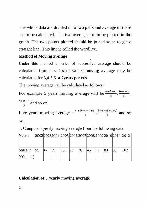
1. Compute 3 yearly moving average from the following data
Years: 2002 2003 2004 2005 2006 2007 2008 2009 2010 2011 2012
Sales(in
000 units)
55 47 59 151 79 36 45 72 83 89 102
Calculation of 3 yearly moving average

15
Year Sales (in 000 units) 3 yearly moving total 3 yearly moving average
2002 55 ‐‐‐‐‐‐‐‐‐‐ ‐‐‐‐‐‐‐‐‐‐‐
2003 47 ‐‐‐‐‐‐‐‐‐‐ ‐‐‐‐‐‐‐‐‐‐
2004 59 161 53.67
2005 151 257 85.67
2006 79 289 96.33
2007 36 216 58.67
2008 45 160 63.33
2009 72 153 51
2010 83 200 66.67
2011 89 244 81.33
2012 102 277 91.33
2. Calculate 5 yearly moving averages
Years: 2000 2001 2002 2003 2004 2005 2006 2007 2008 2009 2010
income
(in ‘000’)
161 127 152 143 144 167 182 179 152 163 159
Solution
Year Income (in 000)
Five yearly
moving total
Five yearly
moving average
2000 161 ‐‐‐‐‐‐‐‐‐‐ ‐‐‐‐‐‐‐‐‐‐‐

16
2001 127 ‐‐‐‐‐‐‐‐‐‐ ‐‐‐‐‐‐‐‐‐‐
2002 152 727 145.4
2003 143 733 146.6
2004 144 788 157.6
2005 167 815 163
2006 182 824 164.8
2007 179 843 168.6
2008 152 835 167
2009 163 ‐‐‐‐‐‐‐‐‐‐ ‐‐‐‐‐‐‐‐‐‐‐
2010 159 ‐‐‐‐‐‐‐‐‐‐ ‐‐‐‐‐‐‐‐‐‐
Calculation of moving average for every periods
1) Calculate the six year moving average
Years: 2000 2001 2002 2003 2004 2005 2006 2007 2008 2009 2010
Demand
(intones)
105 120 115 110 100 130 135 160 155 140 145
Solution

17
Year
Demand
6 years
moving total
6 years
moving
average
Centered
6 years
moving
total
Centered 6
year moving
average
2000 105 ‐‐‐‐‐‐‐ ‐‐‐‐‐‐‐ ‐‐‐‐‐‐‐ ‐‐‐‐‐‐‐
2001 120 ‐‐‐‐‐‐‐‐ ‐‐‐‐‐‐‐‐ ‐‐‐‐‐‐‐‐ ‐‐‐‐‐‐‐‐
2002 115 ‐‐‐‐‐‐‐‐‐ ‐‐‐‐‐‐‐‐‐ ‐‐‐‐‐‐‐‐‐ ‐‐‐‐‐‐‐‐‐
2003 110 680 113.3 231.6 115.8
2004 100 710 118.3 243.3 121.65
2005 130 750 125 256.67 128.34
2006 135 790 131.67 268.34 134.17
2007 160 820 136.67 280.84 140.42
2008 155 865 144.17
2009 140
2010 145
Method of Least Squares
This is a popular method of obtaining trend line. The trend line
obtained through this method is called line of best fit.

18
One trend line is represented as y = a + bx
The value of a and b can be ascertained by solving the following
two normal equations.
∑ y = Na + b∑ x
∑ xy = a∑ x + b∑ x2
Where x represents the time, y represents the value, a and b
are constant and N represent total number.
When the middle year is taken as the origin, then ∑ x = 0, then
normal equation would be
∑ xy = Na
∑ xy = b∑ x2
Hence a = ∑𝑥𝑦
∑𝑥2
1. Following are the data related with the output of a factory for
7 years
Years: 2006 2007 2008 2009 2010 2011 2012
Output (in
tones)
47 64 77 88 97 109 113
Calculate the trend values through the method of least squares
and also forecast the production 2013 and 2015.
Solution

19
Year t Production y x
(t – 2009)
xy
x2
2006 47 ‐3 ‐141 9
2007 64 ‐2 ‐128 4
2008 77 ‐1 ‐77 1
2009 88 0 0 0
2010 97 1 97 1
2011 109 2 218 4
2012 113 3 339 9
595 0 308 28
Here ∑x = 0
A = = ∑𝑦
𝑛
595
7 = 85
b = ∑𝑥𝑦
∑𝑥2 = 308
28 = 11
y = a + bx
2006 ‐ 85 + 11 x ‐3 = 52
20
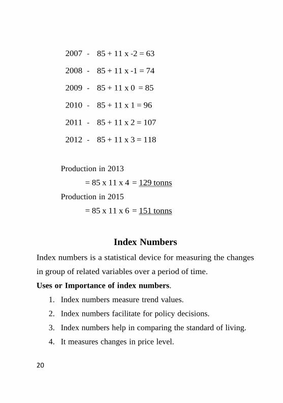
2007 ‐ 85 + 11 x ‐2 = 63
2008 ‐ 85 + 11 x ‐1 = 74
2009 ‐ 85 + 11 x 0 = 85
2010 ‐ 85 + 11 x 1 = 96
2011 ‐ 85 + 11 x 2 = 107
2012 ‐ 85 + 11 x 3 = 118
Production in 2013
= 85 x 11 x 4 = 129 tonns
Production in 2015
= 85 x 11 x 6 = 151 tonns
Index Numbers
Index numbers is a statistical device for measuring the changes
in group of related variables over a period of time.
Uses or Importance of index numbers.
1. Index numbers measure trend values.
2. Index numbers facilitate for policy decisions.
3. Index numbers help in comparing the standard of living.
4. It measures changes in price level.
21
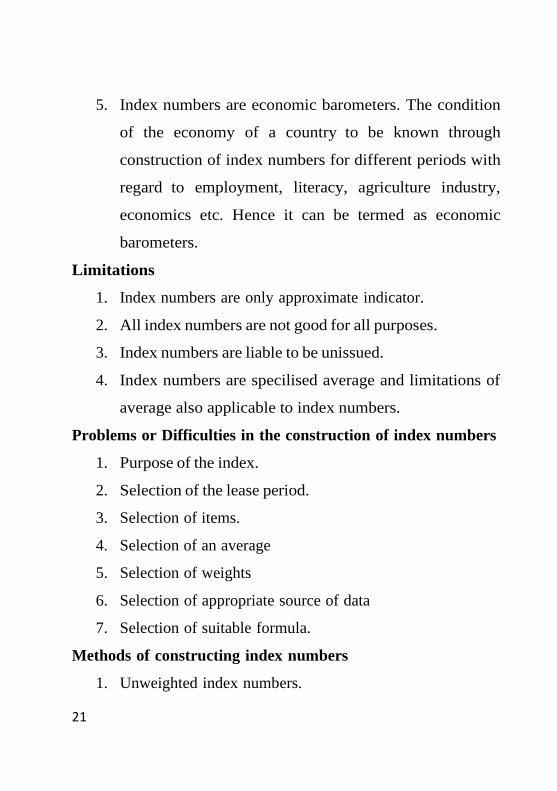
5. Index numbers are economic barometers. The condition
of the economy of a country to be known through
construction of index numbers for different periods with
regard to employment, literacy, agriculture industry,
economics etc. Hence it can be termed as economic
barometers.
Limitations
1. Index numbers are only approximate indicator.
2. All index numbers are not good for all purposes.
3. Index numbers are liable to be unissued.
4. Index numbers are specilised average and limitations of
average also applicable to index numbers.
Problems or Difficulties in the construction of index numbers
1. Purpose of the index.
2. Selection of the lease period.
3. Selection of items.
4. Selection of an average
5. Selection of weights
6. Selection of appropriate source of data
7. Selection of suitable formula.
Methods of constructing index numbers
1. Unweighted index numbers.

22
2. Weighted index numbers.
Unweighted or Simple index numbers
Simple index numbers are those index numbers in which all
items are treated as equally. Simple aggregate and simple
average price relatives are the unweighted index numbers.
1. Simple Aggregate method
P01 = ∑𝑝1
∑𝑝0× 100
P01 = index number
P1 = Price for the current year
P1 = Price for the base year.
2. Simple Average Price Relative Method
P01 = ∑𝐼
𝑛
𝐼 = 𝑝1
𝑝0× 100 , each items can be calculated
Weighted index numbers
In this method quantity consumed is also taken into account.
Such index are-
1. Weighted aggregate method
2. Weighted Average of price relatives
Weighted aggregate method

23
This method is based on the weight of the prices of the selected
commodities. Following are the commonly used methods:
1. Laspeyre’s Method
2. Paasche’s Method
3. Bowley‐Dorbish Method
4. Fishers ideal method
5. Kelly’s Methods
Laspeyre’s Method
P01 = ∑𝑝1𝑞0
∑𝑝0𝑞0× 100
p1 = Price of the current year
q0 = Quantity of the base year
p0 = Price of the base year
Paasche’s Method
P01 = ∑𝑝1𝑞1
∑𝑝0𝑞1× 100
q1 = Quantity of the current year
Fishers Ideal Method
P01 = √𝐿 × 𝑃 × 100
P01 = √∑𝑝1𝑞0
∑𝑝0𝑞1×
∑𝑝1𝑞1
∑𝑝0𝑞1× 100
L = Laspeyres method
P = Paasche’s Method

24
Bowley-Doribish Method
P01 = 𝐿+𝑃
2
Kelly’s Method
P01 = ∑𝑝1𝑞
∑𝑝0𝑞× 100
q = 𝑞0+𝑞1
2
Weighted Average Price Relative Method
Index number = ∑𝐼𝑉
∑𝑣
V = Weight
I = 𝑃1
𝑃0× 100
1. Construct index numbers for 2012 on the basis of the price of
2010
Commodities Price in 2010 Price in 2012
A 115 130
B 72 89
C 54 75
D 60 72
E 80 105
Solution

25
Commodities P0 P1
A 115 130
B 72 89
C 54 75
D 60 72
E 80 105
381 471
P01 = ∑𝑝1
∑𝑝0× 100
P01 = 471
381× 100 = 123.62
2. Calculate simple index number by average relative method.
Items Price of the base year Price of the current
year
A 5 7
B 10 12
C 15 25
D 20 18
E 8 9
Solution

26
Items P0 P1 ie 𝑝1
𝑝0× 100
A 5 7 140
B 10 12 120
C 15 25 166.7
D 20 18 90
E 8 9 112.5
629.2
Index number = ∑𝐼
𝑛 =
629.6
5= 125.84
3. Following are the data related with the prices and quantities
consumed for 2010 and 2012.
Commodity 2010 2012
Price Quantity Price Quantity
Rice 5 15 7 12
Wheat 4 5 6 4
Sugar 7 4 9 3
Tea 52 2 55 2

27
Construct price index numbers by
1. Laspeyre’s method
2. Paasche’s method
3. Bowly’s – Dorbish method
4. Fisher’s method
Solution
Commodity p0 q0 p1 q1 p1q0 p0q0 p1q1 p0q1
Rice 5 15 7 12 105 75 84 60
Wheat 4 5 6 4 30 20 24 16
Sugar 7 4 9 3 36 28 27 21
Tea 12 2 55 2 110 104 110 104
281 227 245 201
1. Laspeyre’s Method
P01 = ∑𝑝1𝑞0
∑𝑝0𝑞0× 100 =
281
227× 100
= 123.79
2. Paascne’s method
P01 = ∑𝑝1𝑞1
∑𝑝0𝑞1× 100 =
245
201× 100

28
= 121.89
3. Bowley – Dorbish Method
P01 = 𝐿+𝑃
2 =
123.79+121.89
2
= 122.84
4. Fisher’s Method
P01 = √𝐿 × 𝑃 = √123.79 × 121.89
= 122.84
4) Calculate index number of price for 2012 on the basis of
2010, from the data given below:
Commodities Weight Price 2010 Price 2012
A 40 16 20
B 25 40 60
C 5 2 2
D 20 5 6
E 10 2 1
Solution

29
𝑃𝑟𝑖𝑐𝑒 𝐼𝑛𝑑𝑒𝑥 𝑁𝑢𝑚𝑏𝑒𝑟 =∑𝐼𝑉
∑𝑣
Commodities V p0 p1 i.e. p1 x 100
p0 IV
A 40 16 20 125 5000
B 25 40 60 150 3750
C 5 2 2 100 500
D 20 5 6 120 2400
E 10 2 1 50 500
100 12150
𝐼𝑛𝑑𝑒𝑥 𝑁𝑢𝑚𝑏𝑒𝑟 =12150
100
5. Construct Price Index
Commodities Index Weight
A 350 5
B 200 2
C 240 3
D 150 1
E 250 2

30
Solution
Commodities V I IV
A 5 350 1750
B 2 200 400
C 3 240 720
D 1 150 150
E 2 250 500
13 3520
𝑃𝑟𝑖𝑐𝑒 𝐼𝑛𝑑𝑒𝑥 𝑁𝑢𝑚𝑏𝑒𝑟 =∑𝐼𝑉
∑𝑣 =
3520
13 = 270.77
Consumer Price index number of cost of Living index number
or Retail Price index number
Consumer Price index number is also known as copy of Living
Index number or Retails Price index number. It is the ration of
the monetary expenditures of an individual which secure him
the standard of living or total utility in two situations differing
only in respect of prices. It represents the average change in
prices over a period of time, paid by the consumer for goods and
services.
Steps in the construction of Consumer Price Index
1. Determination of the class people for whom the index
31
number is to construct.
2. Selection of Basic period
3. Conducting family budget enquiry
4. Obtaining price quotation
5. Selecting proper weights
6. Selection of suitable methods for constructing index.
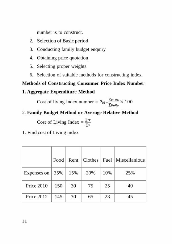
Methods of Constructing Consumer Price Index Number
1. Aggregate Expenditure Method
Cost of living Index number = P01 = ∑𝑝1𝑞0
∑𝑝0𝑞0× 100
2. Family Budget Method or Average Relative Method
Cost of Living Index = ∑𝐼𝑉
∑𝑣
1. Find cost of Living index
Food
Rent
Clothes
Fuel
Miscellanious
Expenses on 35% 15% 20% 10% 25%
Price 2010 150 30 75 25 40
Price 2012 145 30 65 23 45

32
What changes the cost of living of 2012 as compare to 2010?
Solution
Expenses V p0 p1 I IV
Food 35 150 145 96.67 3383.45
Rent 15 30 30 100 1500
Cloth 20 75 65 86.67 1733
Fuel 10 25 23 92 920
Misc. 20 40 45 112.50 2250
9786.85
Cost of Living Index = ∑𝐼𝑉
∑𝑣=
9786.85
100= 97.87
33
Module III: Correlation and Regression Analysis
In practice, we may come across with lot of situations which need
statistical analysis of either one or more variables. The data
concerned with one variable only is called univariate data. For
Example: Price, income, demand, production, weight, height
marks etc are concerned with one variable only. The analysis of
such data is called univariate analysis.
The data concerned with two variables are called bivariate data.
For example: rainfall and agriculture; income and consumption;
price and demand; height and weight etc. The analysis of these
two sets of data is called bivariate analysis.
The date concerned with three or more variables are called
multivariate date. For example: agricultural production is
influenced by rainfall, quality of soil, fertilizer etc.
The statistical technique which can be used to study the
relationship between two or more variables is called correlation
analysis.
Definition:
Two or more variables are said to be correlated if the change in
one variable results in a corresponding change in the other
variable.

34
According to Simpson and Kafka, “Correlation analysis deals
with the association between two or more variables”.
Lunchou defines, “Correlation analysis attempts to determine the
degree of relationship between variables”.
Boddington states that “Whenever some definite connection exists
between two or more groups or classes of series of data, there is
said to be correlation.”
In nut shell, correlation analysis is an analysis which helps to
determine the degree of relationship exists between two or more
variables.
Correlation Coefficient:
Correlation analysis is actually an attempt to find a numerical
value to express the extent of relationship exists between two or
more variables. The numerical measurement showing the degree
of correlation between two or more variables is called correlation
coefficient. Correlation coefficient ranges between -1 and +1.
Significance of Correlation Analysis
1. Correlation analysis is of immense use in practical life
because of the following reasons:
2. Correlation analysis helps us to find a single figure to
measure the degree of relationship exists between the
variables. Correlation analysis helps to understand the

35
economic behavior.
3. Correlation analysis enables the business executives to
estimate cost, price and other variables.
4. Correlation analysis can be used as a basis for the study of
regression. Once we know that two variables are closely
related, we can estimate the value of one variable if the
value of other is known.
5. Correlation analysis helps to reduce the range of
uncertainty associated with decision making. The
prediction based on correlation analysis is always near to
reality.
6. It helps to know whether the correlation is significant or
not. This is possible by comparing the correlation co-
efficient with 6PE. It ‘r’ is more than 6 PE, the correlation
is significant.
Classification of Correlation
Correlation can be classified in different ways. The following are
the most important classifications
1. Positive and Negative correlation
2. Simple, partial and multiple correlation
3. Linear and Non-linear correlation

36
Positive and Negative Correlation
Positive Correlation
When the variables are varying in the same direction, it is called
positive correlation. In other words, if an increase in the value of
one variable is accompanied by an increase in the value of other
variable or if a decrease in the value of one variable is
accompanied by a decree se in the value of other variable, it is
called positive correlation.
Eg: 1) A: 10 20 30 40 50
B: 80 100 150 170 200
2) X: 78 60 52 46 38
Y: 20 18 14 10 5
Negative Correlation:
When the variables are moving in opposite direction, it is called
negative correlation. In other words, if an increase in the value of
one variable is accompanied by a decrease in the value of other
variable or if a decrease in the value of one variable is
accompanied by an increase in the value of other variable, it is
called negative correlation.
Eg: 1) A: 5 10 15 20 25
B: 16 10 8 6 2
2) X: 40 32 25 20 10

37
Y: 2 3 5 8 12
Simple, Partial and Multiple correlation
Simple Correlation
In a correlation analysis, if only two variables are studied it is
called simple correlation. Eg. the study of the relationship
between price & demand, of a product or price and supply of a
product is a problem of simple correlation.
Multiple correlation
In a correlation analysis, if three or more variables are studied
simultaneously, it is called multiple correlation. For example,
when we study the relationship between the yield of rice with both
rainfall and fertilizer together, it is a problem of multiple
correlation.
Partial correlation
In a correlation analysis, we recognize more than two variable, but
consider one dependent variable and one independent variable and
keeping the other Independent variables as constant. For example
yield of rice is influenced b the amount of rainfall and the amount
of fertilizer used. But if we study the correlation between yield of
rice and the amount of rainfall by keeping the amount of fertilizers
used as constant, it is a problem of partial correlation.
Linear and Non-linear correlation

38
Linear Correlation
In a correlation analysis, if the ratio of change between the two
sets of variables is same, then it is called linear correlation.
For example when 10% increase in one variable is accompanied
by 10% increase in the other variable, it is the problem of linear
correlation.
X: 10 15 30 60
Y: 50 75 150 300
Here the ratio of change between X and Y is the same. When we
plot the data in graph paper, all the plotted points would fall on a
straight line.
Non-linear correlation
In a correlation analysis if the amount of change in one variable
does not bring the same ratio of change in the other variable, it is
called non linear correlation.
X: 2 4 6 10 15
Y: 8 10 18 22 26
Here the change in the value of X does not being the same
proportionate change in the value of Y.
This is the problem of non-linear correlation, when we plot the
data on a graph paper, the plotted points would not fall on a
straight line.

39
Degrees of correlation
Correlation exists in various degrees
Perfect positive correlation
If an increase in the value of one variable is followed by the same
proportion of increase in other related variable or if a decrease in
the value of one variable is followed by the same proportion of
decrease in other related variable, it is perfect positive correlation.
eg: if 10% rise in price of a commodity results in 10% rise in its
supply, the correlation is perfectly positive. Similarly, if 5% full
in price results in 5% fall in supply, the correlation is perfectly
positive.
Perfect Negative correlation
If an increase in the value of one variable is followed by the same
proportion of decrease in other related variable or if a decrease in
the value of one variable is followed by the same proportion of
increase in other related variably it is Perfect Negative Correlation.
For example if 10% rise in price results in 10% fall in its demand
the correlation is perfectly negative. Similarly if 5% fall in price
results in 5% increase in demand, the correlation is perfectly
negative.
Limited Degree of Positive correlation:

40
When an increase in the value of one variable is followed by a non
-proportional increase in other related variable, or when a decrease
in the value of one variable is followed by a nonproportional
decrease in other related variable, it is called limited degree of
positive correlation.
For example, if 10% rise in price of a commodity results in 5%
rise in its supply, it is limited degree of positive correlation.
Similarly if 10% fall in price of a commodity results in 5% fall in
its supply, it is limited degree of positive correlation.
Limited degree of Negative correlation
When an increase in the value of one variable is followed by a
non-proportional decrease in other related variable, or when a
decrease in the value of one variable is followed by
anonproportional increase in other related variable, it is called
limited degree of negative correlation.
For example, if 10% rise in price results in 5% fall in its demand,
it is limited degree of negative correlation. Similarly, if 5% fall in
price results in 10% increase in demand, it is limited degree of
negative correlation.
Zero Correlation (Zero Degree correlation)
If there is no correlation between variables it is called zero
correlation. In other words, if the values of one variable cannot be
41
associated with the values of the other variable, it is zero
correlation.
Methods of measuring correlation
Correlation between 2 variables can be measured by graphic
methods and algebraic methods.
I Graphic Methods
a. Scatter Diagram
b. Correlation graph
II Algebraic methods (Mathematical methods or statistical
methods or Co-efficient of correlationmethods):
a. Karl Pearson’s Co-efficient of correlation
b. Spear mans Rank correlation method
c. Concurrent deviation method
Scatter Diagram
This is the simplest method for ascertaining the correlation
between variables. Under this method all the values of the two
variable are plotted in a chart in the form of dots. Therefore, it is
also known as dot chart. By observing the scatter of the various
dots, we can form an idea that whether the variables are related or
not.

42
A scatter diagram indicates the direction of correlation and tells us
how closely the two variables under study are related. The greater
the scatter of the dots, the lower is the relationship.
Figure 1 :Perfect Positive Correlation
0
2
4
6
8
10
12
0 1 2 3 4 5 6

43
Figure 1 :Perfect Negative Correlation
Merits of Scatter Diagram method
1. It is a simple method of studying correlation between
variables.
2. It is a non-mathematical method of studying correlation
between the variables. It does not require any
mathematical calculations.
3. It is very easy to understand. It gives an idea about the
correlation between variables even to a layman.
-12
-10
-8
-6
-4
-2
0

44
4. It is not influenced by the size of extreme items.
5. Making a scatter diagram is, usually, the first step in
investigating the relationship between two variables.
Demerits of Scatter diagram method
It gives only a rough idea about the correlation between variables.
The numerical measurement of correlation co-efficient cannot be
calculated under this method.
It is not possible to establish the exact degree of relationship
between the variables.
Correlation graph Method
Under correlation graph method the individual values of the two
variables are plotted on a graph paper. Then dots relating to these
variables are joined separately so as to get two curves. By
examining the direction and closeness of the two curves, we can
infer whether the variables are related or not. If both the curves
are moving in the same direction( either upward or downward)
correlation is said to be positive. If the curves are moving in the
opposite directions, correlation is said to be negative.
Merits of Correlation Graph Method
1. This is a simple method of studying relationship between
the variable
2. This does not require mathematical calculations.

45
3. This method is very easy to understand
Demerits of correlation graph method:
1. A numerical value of correlation cannot be calculated.
2. It is only a pictorial presentation of the relationship
between variables.
3. It is not possible to establish the exact degree of
relationship between the variables.
Karl Pearson’s Co-efficient of Correlation
Karl Pearson’s Coefficient of Correlation is the most popular
method among the algebraic methods for measuring correlation.
This method was developed by Prof. Karl Pearson in 1896. It is
also called product moment correlation coefficient.
Pearson’s coefficient of correlation is defined as the ratio of the
covariance between X and Y to the product of their standard
deviations. This is denoted by ‘r’ or rxy
r = Covariance of X and Y
(SD of X) x (SD of Y)
Interpretation of Co-efficient of Correlation
Pearson’s Co-efficient of correlation always lies between +1 and -
The following general rules will help to interpret the Co-efficient
of correlation:
1. When r - +1, It means there is perfect positive relationship

46
between variables.
2. When r = -1, it means there is perfect negative relationship
between variables.
3. When r = 0, it means there is no relationship between the
variables.
4. When ‘r’ is closer to +1, it means there is high degree of
positive correlation between variables.
5. When ‘r’ is closer to – 1, it means there is high degree of
negative correlation between variables.
6. When ‘r’ is closer to ‘O’, it means there is less relationship
between variables.
Properties of Pearson’s Co-efficient of Correlation
1. If there is correlation between variables, the Co-efficient of
correlation lies between +1 and -1.
2. If there is no correlation, the coefficient of correlation is
denoted by zero (ie r=0)
3. It measures the degree and direction of change
4. If simply measures the correlation and does not help to
predict cansation.
5. It is the geometric mean of two regression co-efficients.
i.e r =√𝑏xy . 𝑏𝑦𝑥

47
Computation of Pearson’s Co-efficient of correlation:
Pearson’s correlation co-efficient can be computed in different
ways. They are:
1. Arithmetic mean method
2. Assumed mean method
3. Direct method
Arithmetic mean method:-
Under arithmetic mean method, co-efficient of correlation is
calculated by taking actual mean.
r = Σ(𝑥−𝑥)(𝑦−𝑦)
√Σ(𝑥−𝑥)2 Σ(𝑦−𝑦)2
or r =Σxy
√Σ𝑥2 Σy2
Calculate Pearson’s co-efficient of correlation between age and
playing habits of students:
Age: 20 21 22 23 24 25
No. of students 500 400 300 240 200 160
Regular players 400 300 180 96 60 24
Let X = Age and Y = Percentage of regular players
Percentage of regular players can be calculated as follows:-
400 x 100 = 80; 300 x 100 = 75; 180 x 100 = 60; 96 x 100 =
40 ,
500 400 300 240

48
60 x 100 = 30; and 24 x 100 = 15
20 160
Pearson’s Coefficient of Correlation (r) = Σ(𝑥−𝑥)(𝑦−𝑦)
√Σ(𝑥−𝑥)2 Σ(𝑦−𝑦)2
Computation of Pearson’s Coefficient of
correlation
Age
x
% of
Regular
Player
y
(x-
22.5)
(y-
50) (x-𝑥) (y-𝑦) (x-𝑥)2 (y-𝑦)2
20 80 -2.5 30 -75.0 6.25 900
21 75 -1.5 25 -37.5 2.25 625
22 60 -0.5 10 - 5.0 0.25 100
23 40 0.5 -10 - 5.0 0.25 100
24 30 1.5 -20 -30.0 2.25 400
25 15 2.5 -35 -87.5 6.25 1225
135 300 -240 17.50 3350
49
𝑥 = Σ𝑥
𝑁 =
135
6 = 22.5
𝑦 = Σy
𝑁 =
300
6 = 50
r = −240
√17.5×3350 =
−240
√58625 =
−240
√242.126 = −0.9912
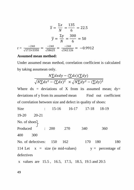
Assumed mean method:
Under assumed mean method, correlation coefficient is calculated
by taking assumean only.
𝑁∑𝑑𝑥𝑑𝑦 − (∑𝑑𝑥)(∑𝑑𝑦)
√𝑁∑𝑑𝑥2 − (∑𝑑𝑥)2 × √𝑁∑𝑑𝑦2 − (∑𝑑𝑦)2
Where dx = deviations of X from its assumed mean; dy=
deviations of y from its assumed mean Find out coefficient
of correlation between size and defect in quality of shoes:
Size : 15-16 16-17 17-18 18-19
19-20 20-21
No. of shoes
Produced : 200 270 340 360
400 300
No. of defectives: 150 162 170 180 180
114 Let x = size (ie mid-values) y = percentage of
defectives
x values are 15.5 , 16.5, 17.5, 18.5, 19.5 and 20.5
50
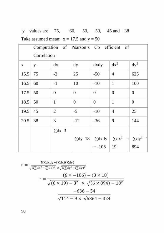
y values are 75, 60, 50, 50, 45 and 38
Take assumed mean: x = 17.5 and y = 50
Computation of Pearson’s Co efficient of
Correlation
x y dx dy dxdy dx2 dy2
15.5 75 -2 25 -50 4 625
16.5 60 -1 10 -10 1 100
17.5 50 0 0 0 0 0
18.5 50 1 0 0 1 0
19.5 45 2 -5 -10 4 25
20.5 38 3 -12 -36 9 144
∑dx 3
∑dy 18 ∑dxdy
= -106
∑dx2 =
19
∑dy2 =
894
r =N∑dxdy−(∑dx)(∑dy)
√N∑dx2−(∑dx)2 ×√N∑dy2−(∑dy)2
r =(6 × −106) − (3 × 18)
√(6 × 19) − 32 × √(6 × 894) − 182
−636 − 54
√114 − 9 × √5364 − 324

51
= −690
√105× √5040=
−690
727.46 = -0.9485
Direct Method:
Under direct method, coefficient of correlation is calculated
without taking actual mean or assumed mean
r =N∑xy − (∑x)(∑y)
√N∑x2 − (∑x)2 × √N∑y2 − (∑y)2
From the following data, compute Pearson’s correlation
coefficient:
Price : 10 12 14 15 19
Demand (Qty) 40 41 48 60 50
Let us take price = x and demand = y
Computation of Pearson’s Coefficient of Correlation
Price (x)
Demand
(y) xy x2 y2
10 40 400 100 1600
12 41 492 144 1681
14 48 672 196 2304
15 60 900 225 3600
19 50 950 361 2500

52
∑x = 70 ∑y = 239 ∑xy = 3414 ∑x2 1026 ∑y2=11685
r =N∑xy−(∑x)(∑y)
√N∑x2−(∑x)2 ×√N∑y2−(∑y)2 =
r =(5 × 3414) − (70 × 239)
√(5 × 1026) − 702 × √(5 × 11685) − 2392
r =17070−16730
√230 × √1304 = 0.621
Probable Error and Coefficient of Correlation
Probable error (PE) of the Co-efficient of correlation is a statistical
device which measures the reliability and dependability of the
value of co-efficient of correlation.
Probable Error = 2
3 standard error
= 0.6745 x standard error
Standard Error (SE) = 1−𝑟2
√𝑛
∴ 𝑃𝐸 = 0.6745 ×1 − 𝑟2
√𝑛
If the value of coefficient of correlation ( r) is less than the PE,
then there is no evidence of correlation.
If the value of ‘r’ is more than 6 times of PE, the correlation is
certain and significant.
53
By adding and submitting PE from coefficient of correlation, we
can find out the upper and lower limits within which the
population coefficient of correlation may be expected to lie.
Uses of PE:
1. PE is used to determine the limits within which the
population coefficient of correlation may be expected to
lie.
2. It can be used to test whether the value of correlation
coefficient of a sample is significant with that of the
population
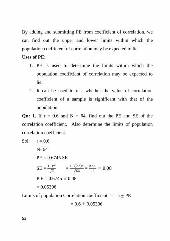
Qn: 1. If r = 0.6 and N = 64, find out the PE and SE of the
correlation coefficient. Also determine the limits of population
correlation coefficient.
Sol: r = 0.6
N=64
PE = 0.6745 SE
SE = 1−𝑟2
√𝑛 =
1−(0.6)2
√64 =
0.64
8= 0.08
P.E = 0.6745 × 0.08
= 0.05396
Limits of population Correlation coefficient = r± PE
= 0.6 ± 0.05396

54
= 0.54604 to 0.6540
Qn. 2 r and PE have values 0.9 and 0.04 for two series. Find n.
Sol: PE = 0.04
= 0.6745 1−𝑟2
√𝑛=0.04
1−092
√𝑛 =
0.04
0.6745
= 1−0.81
√𝑛= 0.0593
= 0.19
√𝑛= 0.0593
= 0.0593×√𝑛 = 0.19
= √𝑛 = 0.19
0.0593
= N = 3.22 = 10. 266
N = 10
Coefficient of Determination
One very convenient and useful way of interpreting the value of
coefficient of correlation is the use of the square of coefficient of
correlation. The square of coefficient of correlation is called
coefficient of determination.
Coefficient of determination = r2
Coefficient of determination is the ratio of the explained variance
to the total variance.
For example, suppose the value of r = 0.9, then r2 = 0.81=81%

55
This means that 81% of the variation in the dependent variable has
been explained by (determined by) the independent variable. Here
19% of the variation in the dependent variable has not been
explained by the independent variable. Therefore, this 19% is
called coefficient of non-determination.
Coefficient of non-determination (K2) = 1 – r2
K2 = 1- coefficient of determination
Qn: Calculate coefficient of determination and non-determination
if coefficient of correlation is 0.8
Sol:- r =0.8
Coefficient of determination = r2
= 0.82 =0.64 =
64%
Co efficient of non-determination = 1 – r2
= 1- 0.64
= 0.36
= 36%
Merits of Pearson’s Coefficient of Correlation:-
1. This is the most widely used algebraic method to measure
coefficient of correlation.
2. It gives a numerical value to express the relationship

56
between variables
3. It gives both direction and degree of relationship between
variables
4. It can be used for further algebraic treatment such as
coefficient of determination coefficient of non-
determination etc.
5. It gives a single figure to explain the accurate degree of
correlation between two variables
Demerits of Pearson’s Coefficient of correlation
1. It is very difficult to compute the value of coefficient of
correlation.
2. It is very difficult to understand
3. It requires complicated mathematical calculations
4. It takes more time
5. It is unduly affected by extreme items
6. It assumes a linear relationship between the variables. But
in real life situation, it may not be so.
Spearman’s Rank Correlation Method
Pearson’s coefficient of correlation method is applicable when
variables are measured in quantitative form. But there were many
cases where measurement is not possible because of the qualitative
nature of the variable. For example, we cannot measure the

57
beauty, morality, intelligence, honesty etc in quantitative terms.
However it is possible to rank these qualitative characteristics in
some order.
The correlation coefficient obtained from ranks of the variables
instead of their quantitative measurement is called rank
correlation. This was developed by Charles Edward Spearman in
1904. Spearman’s coefficient correlation (R) = 1 −6∑𝐷2
𝑁3− 𝑁
Where D = difference of ranks between the two variables
N = number of pairs
Qn: Find the rank correlation coefficient between poverty and
overcrowding from the information given below:
Town: A B C D E F G H I
J
Poverty: 17 13 15 16 6 11 14 9
7 12
Over crowing:36 46 35 24 12 18 27 22 2
8
Sol: Here ranks are not given. Hence we have to assign ranks
R = 1 −6∑𝐷2
𝑁3− 𝑁
N = 10

58
Computation of rank correlation Co-efficient
Town Poverty Over
crowding R1 R2 D D2
A 17 36 1 2 1 1
B 13 46 5 1 4 16
C 15 35 3 3 0 0
D 16 24 2 5 3 9
E 6 12 10 8 2 4
F 11 18 7 7 0 0
G 14 27 4 4 0 0
H 9 22 8 6 2 4
I 7 2 9 10 1 1
J 12 8 6 9 3 9
∑𝐷2 44

59
R = 1 −6×44
103− 10 = 1 −
264
990 = 1- 0.2667
=0.7333
Qn:- Following were the ranks given by three judges in a beauty
context. Determine which pair of judges has the nearest approach
to Common tastes in beauty.
Judge I: 1 6 5 10 3 2 4 9 7 8
Judge I: 3 5 8 4 7 10 2 1 6 9
Judge I: 6 4 9 8 1 2 3 10 5 7
R = 1 −6∑𝐷2
𝑁3− 𝑁 N= 10
Computation of Spearman’s Rank Correlation
Coefficient
Judge
I
(R1)
Judge
II
(R2)
Jud
ge
III
(R3)
R1-
R2
(D1
)
R2-
R3
(D2)
R1-
R3
(D3)
D12
D22
D32
1 3 6 2 3 5 4 9 25
6 5 4 1 1 2 1 1 4
5 8 9 3 1 4 9 1 16
10 4 8 6 4 2 36 16 4

60
3 7 1 4 6 2 16 36 4
2 10 2 8 8 0 64 64 0
4 2 3 2 1 1 4 1 1
9 1 10 8 9 1 64 81 1
7 6 5 1 1 2 1 1 4
8 9 7 1 2 1 1 4 1
∑D2 200 214 60
R = 1 −6∑𝐷2
𝑁3− 𝑁
Rank correlation coefficient between I & II =1 - 6×200
103− 10
= 1 − 1200
990
= 1- 1.2121
= - 0.2121
Rank correlation Coefficient between II & III judges= 1 −6×214
103− 10
= 1 − 1284
990
=-0.297
Rank correlation coefficient between I& II judges = 1 −6×60
103− 10
= 1 −360
990

61
= 1- 0.364
= 0.636
The rank correlation coefficient in case of I& III judges is greater
than the other two pairs. Therefore, judges I & III have highest
similarity of thought and have the nearest approach to common
taste in beauty.
Qn: The Co-efficient of rank correlation of the marks obtained by
10 students in statistics & English was 0.2. It was later
discovered that the difference in ranks of one of the students was
wrongly takes as 7 instead of 9 find the correct result.
R = 0.2
= 1 −6∑𝐷2
𝑁3− 𝑁 = 0.2
= 1−0.2
1 =
6∑𝐷2
103− 10
= 0.8
1 =
6∑𝐷2
990
= 6∑𝐷2 = 990 ×0.8 = 792
Correct ∑𝐷2 = 792
6 =132- 72 +92 = 164
Correct R = 1 −6∑𝐷2
𝑁3− 𝑁 = 1 −
6×164
103− 10
= 1 − 984
990 = 1 - 0.9939
= 0.0061

62
Qn: The coefficient of rank correlation between marks in English
and maths obtained by a group students is 0.8. If the sum of the
squares of the difference in ranks is given to be 33, find the
number of students in the group.
Sol: R = 1 −6∑𝐷2
𝑁3− 𝑁 = 0.8
ie, = 1 −6×33
𝑁3− 𝑁 = 0.8
= 1 − 0.8 =6×33
𝑁3− 𝑁
= 0.2× (N3 -N) = 198
= N3 -N = 198
0.2 = 990
N = 10
Computation of Rank Correlation Coefficient when Ranks are
Equal
There may be chances of obtaining same rank for two or more
items. In such a situation, it is required to give average rank for
all. Such items. For example, if two observations got 4th rank,
each of those observations should be given the rank 4.5
(i.e4+5
2=4.5)
Suppose 4 observations got 6th rank, here we have to assign the
rank, 7.5 (ie.6+7+8+9
4 ) to each of the 4 observations.

63
When there is an equal rank, we have to apply the following
formula to compute rank correlation coefficient:-
𝑅 = 1 −6 [Σ𝐷2 +
112 (𝑚3 − 𝑚) +
112 (𝑚3 − 𝑚)+. . . … ]
𝑁3 − 𝑁
Where D – Difference of rank in the two series
N - Total number of pairs
m - Number of times each rank repeats
Qn:- Obtain rank correlation co-efficient for the data:-
X : 68 64 75 50 64 80 75 40
55 64
Y: 62 58 68 45 81 60 68 48
50 70
Here, ranks are not given we have to assign ranks Further; this is
the case of equal ranks.
∴ 𝑅 = 1 −6 [Σ𝐷2 +
112 (𝑚3 − 𝑚) +
112 (𝑚3 − 𝑚)+. . . … ]
𝑁3 − 𝑁
Computation of rank correlation coefficient
x y R1 R2 D(R1-R2) D2
68 62 4 5 1 1

64
64 58 6 7 1 1
75 68 2.5 3.5 1 1
50 45 9 10 1 1
54 81 6 1 5 25
80 60 1 6 5 25
75 68 2.5 3.5 1 1
40 48 10 9 1 1
55 50 8 8 0 0
64 70 6 2 4 16
ΣD2 72
R= = 1 −6[72+
1
12(23−2)+
1
12(33−3)+
1
12(23−2)]
103 −10
= 1 −6[72+
1
12+2+
1
12]
103 −10
= 1 −6 × [72 + 3]
990
=1 − 6×75
990
= 1 − 450
990 = 1- 0.4545
= 0.5455

65
Merits of Rank Correlation method
1. Rank correlation coefficient is only an approximate
measure as the actual values are not used for calculations
2. It is very simple to understand the method.
3. It can be applied to any type of data, ie quantitative and
qualitative
4. It is the only way of studying correlation between
qualitative data such as honesty, beauty etc.
5. As the sum of rank differences of the two qualitative data
is always equal to zero, this method facilitates a cross
check on the calculation.
Demerits of Rank Correlation method
1. Rank correlation coefficient is only an approximate
measure as the actual values are not used for calculations.
2. It is not convenient when number of pairs (ie. N) is large
3. Further algebraic treatment is not possible
4. Combined correlation coefficient of different series cannot
be obtained as in the case of mean and standard deviation.
In case of mean and standard deviation, it is possible to
compute combine arithematic mean and combined standard
deviation.
66
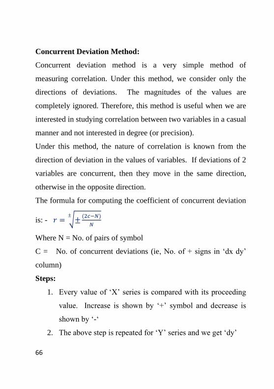
Concurrent Deviation Method:
Concurrent deviation method is a very simple method of
measuring correlation. Under this method, we consider only the
directions of deviations. The magnitudes of the values are
completely ignored. Therefore, this method is useful when we are
interested in studying correlation between two variables in a casual
manner and not interested in degree (or precision).
Under this method, the nature of correlation is known from the
direction of deviation in the values of variables. If deviations of 2
variables are concurrent, then they move in the same direction,
otherwise in the opposite direction.
The formula for computing the coefficient of concurrent deviation
is: - 𝑟 = √±(2𝑐−𝑁)
𝑁
±
Where N = No. of pairs of symbol
C = No. of concurrent deviations (ie, No. of + signs in ‘dx dy’
column)
Steps:
1. Every value of ‘X’ series is compared with its proceeding
value. Increase is shown by ‘+’ symbol and decrease is
shown by ‘-‘
2. The above step is repeated for ‘Y’ series and we get ‘dy’

67
3. Multiply ‘dx’ by ‘dy’ and the product is shown in the next
column. The column heading is ‘dxdy’.
4. Take the total number of ‘+’ signs in ‘dxdy’ column. ‘+’
signs in ‘dxdy’ column denotes the concurrent deviations,
and it is indicated by ‘C’.
5. Apply the formula:
𝑟 = √±(2𝑐−𝑁)
𝑁
±
If 2c>N, then r = +ve and if 2c < N, then r = -ve .
Qn:- Calculate coefficient if correlation by concurrent deviation
method:-
Year : 2003 2004 2005 2006 2007 2008 2009
2010 2011
Supply : 160 164 172 182 166 170 178
192 186
Price : 292 280 260 234 266 254 230
190 200
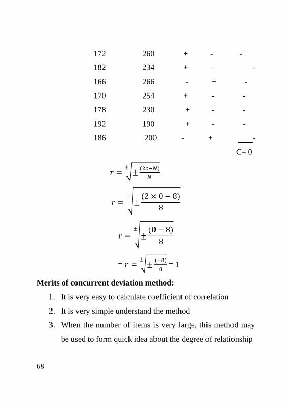
Sol: Computation of coefficient of concurrent
Deviation
Supply (x) Price (y) dx dy dxdy
160 292 + - -
164 280 + - -
68
172 260 + - -
182 234 + - -
166 266 - + -
170 254 + - -
178 230 + - -
192 190 + - -
186 200 - + -
C= 0
𝑟 = √±(2𝑐−𝑁)
𝑁
±
𝑟 = √±(2 × 0 − 8)
8
±
𝑟 = √±(0 − 8)
8
±
= 𝑟 = √±(−8)
8
±
= 1
Merits of concurrent deviation method:
1. It is very easy to calculate coefficient of correlation
2. It is very simple understand the method
3. When the number of items is very large, this method may
be used to form quick idea about the degree of relationship

69
4. This method is more suitable, when we want to know the
type of correlation (ie, whether positive or negative).
Demerits of concurrent deviation method:
1. This method ignores the magnitude of changes. ie. Equal
weight is give for small and big changes.
2. The result obtained by this method is only a rough
indicator of the presence or absence of correlation
3. Further algebraic treatment is not possible
4. Combined coefficient of concurrent deviation of different
series cannot be found as in the case of arithmetic mean
and standard deviation.

70
Regression Analysis
Correlation analysis analyses whether two variables are correlated
or not. After having established the fact that two variables are
closely related, we may be interested in estimating the value of
one variable, given the value of another. Hence, regression
analysis means to analyse the average relationship between two
variables and thereby provides a mechanism for estimation or
predication or forecasting.
The term ‘Regression” was firstly used by Sir Francis Galton in
1877. The dictionary meaning of the term ‘regression” is
“stepping back” to the average.
Definition:
“Regression is the measure of the average relationship between
two or more variables in terms of the original units of the date”.
“Regression analysis is an attempt to establish the nature of the
relationship between variables-that is to study the functional
relationship between the variables and thereby provides a
mechanism for prediction or forecasting”.
It is clear from the above definitions that Regression Analysis is a
statistical device with the help of which we are able to estimate the

71
unknown values of one variable from known values of another
variable. The variable which is used to predict the another
variable is called independent variable (explanatory variable) and,
the variable we are trying to predict is called dependent variable
(explained variable).
The dependent variable is denoted by X and the independent
variable is denoted by Y.
The analysis used in regression is called simple linear regression
analysis. It is called simple because three is only one predictor
(independent variable). It is called linear because, it is assumed
that there is linear relationship between independent variable and
dependent variable.
Types of Regression:-
There are two types of regression. They are linear regression and
multiple regression.
Linear Regression:
It is a type of regression which uses one independent variable to
explain and/or predict the dependent variable.
Multiple Regression:
It is a type of regression which uses two or more independent
variable to explain and/or predict the dependent variable.

72
Regression Lines:
Regression line is a graphic technique to show the functional
relationship between the two variables X and Y. It is a line which
shows the average relationship between two variables X and Y.
If there is perfect positive correlation between 2 variables, then
the two regression lines are winding each other and to give one
line. There would be two regression lines when there is no perfect
correlation between two variables. The nearer the two regression
lines to each other, the higher is the degree of correlation and the
farther the regression lines from each other, the lesser is the degree
of correlation.
Properties of Regression lines:-
1. The two regression lines cut each other at the point of
average of X and average of Y ( i.eX and Y )
2. When r = 1, the two regression lines coincide each other
and give one line.
3. When r = 0, the two regression lines are mutually
perpendicular.
Regression Equations (Estimating Equations)
Regression equations are algebraic expressions of the regression
lines. Since there are two regression lines, therefore two
regression equations. They are :-

73
Regression Equation of X on Y:-
This is used to describe the variations in the values of X for
given changes in Y.
Regression Equation of Y on X :-
This is used to describe the variations in the value of Y for
given changes in X.
Least Square Method of computing Regression Equation:
The method of least square is an objective method of determining
the best relationship between the two variables constituting a
bivariate data. To find out best relationship means to determine
the values of the constants involved in the functional relationship
between the two variables. This can be done by the principle of
least squares:
The principle of least squares says that the sum of the squares of
the deviations between the observed values and estimated values
should be the least. In other words, Σ will be the minimum.
With a little algebra and differential calculators we can develop
some equations (2 equations in case of a linear relationship) called
normal equations. By solving these normal equations, we can find
out the best values of the constants.
Regression Equation of Y on X:-

74
Y = a + bx
The normal equations to compute ‘a’ and ‘b’ are: -
∑y = Na + b∑x
∑xy =a∑x + b∑x2
Regression Equation of X on Y:-
X = a + by
The normal equations to compute ‘a’ and ‘b’ are:-
∑x = Na + b∑y
∑xy =a∑y + b∑y2
Qn:- Find regression equations x and y and y on x from the
following:-
X: 25 30 35 40 45 50 55
Y: 18 24 30 36 42 48 54
Sol: Regression equation x on y is:
x= a + by
Normal equations are:
∑x = Na + b∑y
∑xy =a∑y + b∑y2
Computation of Regression Equations
x y x2 y2 xy

75
25 18 625 324 450
30 24 900 576 720
35 30 1225 900 1050
40 36 1600 1296 1440
45 42 2025 1764 1890
50 48 2500 2304 2400
55 54 3025 2916 2970
Σx= 280 Σy=
252 Σx2 =11900
Σy2=
10080 Σxy 10920
280 = 7a+ 252 b ------------ (1)
10920 = 252a+10080 b ----------- (2)
Eq. 1×36 10080 = 252a + 9072b ------------- (3)
10920= 252a + 10080b ------------- (2)
(2) × (3) 840 = 0 + 1008 b
1008 b = 840
b = 840
1008= 0.83
Substitute b = 0.83 in equation (1)

76
280 = 7a + (252×0.83)
280 = 7 a + 209.16
7a+ 209.116 = 280
7a = 280-209.160
a = 70.84
7= 10.12
Substitute a = 10.12 and b =0.83 in regression equation:
X = 10.12 + 0.83y
Regression equation Y on X is:
y = a + bx
Normal Equations are:-
∑y = Na + b∑x
∑xy =a∑x + b∑x2
252 = 7a + 280 b ------- (1)
10920 = 280 a+ 11900 b ------- (2)
(1)× 40 → 10080 = 280 a + 11200 b ------- (3)
10920 = 280 a+ 11900 b ------- (2)
(2) – (3) → 840 = 0 + 700 b
700 b = 840
b = 840
700 = 1.2
Substitute b = 1.2 in equation (1)
252 = 7a + (280x1.2)

77
252 = 7a + 336
7a + 336 = 252
7a = 252 – 336 = -84
a = −84
7 = -12
Substitute a = -12 and b = 1.2 in regression equation
y = -12+1.2x
Qn:- From the following bivariate data, you are required to: -
(a) Fit the regression line Y on X and predict Y if x = 20
(b) Fir the regression line X on Y and predict X if y = 10
X: 4 12 8 6 4 4 16 8
Y: 14 4 2 2 4 6 4 12
Computation of regression equations
x y x2 y2 xy
4 14 16 196 56
12 4 144 16 48
8 2 64 4 16
6 2 36 4 12
4 4 16 16 16
4 6 16 36 24

78
16 4 256 16 64
8 12 64 144 96
Σ x= 62 Σy=48 Σx2= 612 Σy2= 432 Σ xy= 332
Regression equation y on x
y = a + bx
Normal equations are:
∑y = Na + b∑x
∑xy =a∑x + b∑x2
48 = 8a + 62 b ………………. (1)
332 = 62a + 612 b …………… (2)
eq. 1×62 → 2,976 = 496a+ 3844b...…...(3)
eq. 2×8 → 2,976 = 496 + 4896b … . . (4)
eq. 3×eq. 4→ 320 = 0+ 1052b
-1052 b = 320
b = 320
−1052
Substitute b = -0.304 in eq (1)
48 = 8a + (62 x -0.304)
48 = 8a + -18.86
48 + 18.86 = 8a
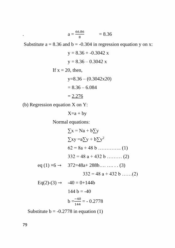
a = 66.86
79
. a = 66.86
8 = 8.36
Substitute a = 8.36 and b = -0.304 in regression equation y on x:
y = 8.36 + -0.3042 x
y = 8.36 – 0.3042 x
If x = 20, then,
y=8.36 – (0.3042x20)
= 8.36 – 6.084
= 2.276
(b) Regression equation X on Y:
X=a + by
Normal equations:
∑x = Na + b∑y
∑xy =a∑y + b∑y2
62 = 8a + 48 b ………….. (1)
332 = 48 a + 432 b ……… (2)
eq (1) ×6 → 372=48a+ 288b…. …. . . (3)
332 = 48 a + 432 b ……(2)
Eq(2)-(3) → -40 = 0+144b
144 b = -40
b =−40
144 = - 0.2778
Substitute b = -0.2778 in equation (1)

80
62 = 8a + (48 0. 2778)
62 = 8a + -13.3344
62+13.3344 = 8 a
8a = 75.3344
a = 75.3344
8 = 9.4168
Substitute a = 9.4168 and b = -0.2778 in regression equation:
x = 9.4168 + -0.2778 y
x = 9.4168 + -0.2778 y
If y=10, then
x=9.4168 – (0.2778x10)
x= 9.4168 – 2.778
x = 6.6388
Regression Coefficient method of computing Regression
Equations:
Regression equations can also be computed by the use of
regression coefficients.
Regression coefficient X on Y is denoted as bxy and that of Y on X
is denoted as byx.
Regression Equation x on y:
x -�̅� = bxy (y -�̅�)

81
ie x -�̅� =𝑟.𝜎𝑥
𝜎𝑦 (y -�̅�)
Regression Equation y on x:
Properties of Regression Coefficient:
1. Both regression co-efficient wills have the same sign i.e.
either they will be positive or negative. It is never possible
that one of the regression co-efficient is negative & other
positive.
2. Since the value of the co-efficient of correlation bxy & byx
cannot exceed one, one of the regression co-efficient must
be less than one or, in other words, both the regression co-
efficient cannot be greater than 1.
3. The coefficient of correlation will have the same sign as
that of regression co-efficient i.e. if regression co-efficient
have a negative sign, r will also be negative and if
regression coefficient have a positive sign, r would be
positive
4. Correlation coefficient is the geometric mean between
regression coefficients
y -�̅� = byx (x -�̅�)
ie y -�̅� =𝑟.𝜎𝑦
𝜎𝑥 (x -�̅�)

82
5. Regression is affected by change of scale & independent of
change in origin
6. The arithmetic mean of bxy & byx is greater than or equal
to coefficient of correlation
7. Since we can find any of these four values, given
the other three
8. If σy = σx, then coefficient correlation equal to regression
coefficient, r = byx = bxy
9. If r=0 the byx and bxy both are zero
10. If byx = bxy then it is equal coefficient of correlation , r =
byx = bxy
Computation of Regression Co-efficients
Regression co-efficients can be calculated in 3 different ways:
1. Actual mean method
2. Assumed mean method
3. Direct method
Actual mean method:-
Regression coefficient x on y (bxy) = Σ𝑥𝑦
Σ𝑦2
Regression coefficient y on x (byx) = = Σ𝑥𝑦
Σ𝑦2
Where x = x –�̅�
y = y –�̅�
x
y
yx rb
=

83
Assumed mean method:
Σd𝑥𝑑𝑦−(Σdx).(Σdy)
Σ𝑑𝑦2−(Σ𝑑𝑦)2 Regression coefficient x on y (bxy)
Σd𝑥𝑑𝑦−(Σdx).(Σdy)
Σ𝑑𝑥2−(Σ𝑑𝑥)2 Regression coefficient y on x (byx)
Where dx = deviation from assumed mean of X
dy = deviation from assumed mean of Y
Direct method:-
NΣ𝑥𝑦−.Σx.Σy)
NΣ𝑦2−(Σ𝑦)2 Regression Coefficient x on y
(bxy)
NΣ𝑥𝑦−.Σx.Σy)
NΣ𝑥2−(Σ𝑥)2 Regression Coefficient y on x
(byx)
Qn:- Following information is obtained from the records of a
business organization:-
Sales ( in ‘000):
91 53 45 76 89 95 80 65
Advertisement Expense ( in ‘000):
15 8 7 12 17 25 20 13
You are required to:-
Compute regression coefficients under 3 methods
Obtain the two regression equations and

84
Estimate the advertisement expenditure for a sale of Rs.
1,20,000
Let x = sales y = Advertisement expenditure
Computation of regression Coefficients under actual mean method
x y x -�̅� y -�̅� xy x2 y2
91 15 16.75 0.375 6.28 280.56 0.14
53 8 -
21.65 -6.625 140.78 451.56 43.89
45 7 -
29.25 -7.625 223.03 855.56 58.14
76 12 1.75 -2,625 -4.59 3.06 6.89
89 17 14.75 -2.375 35.03 217.56 5.64
95 25 20.75 10.375 215.28 430.56 107.64
80 20 5.75 5.375 30.91 33.06 28.89
65 13 -9.25 -1.625 15.03 85.56 2.64
Σ x=
594
Σy=
117 Σxy=661.75
Σx2=
2357.48 Σy2=253.87
X ̅̅ ̅= ∑𝑥
𝑁 =
294
8= 74.25

85
Y ̅ = ∑𝑦
𝑁=
117
8= 14.625
Regression Coefficient x on y
(bxy) ∑𝑥𝑦
∑𝑦2=
661.75
253.87= 2.61
∑𝑥𝑦
∑𝑥2=
661.75
2357.48= 0.28 Regression Coefficient y on x
byx)
Computation of Regression Coefficient under assumed mean
method
x y x-70 y-15 (dy) dxdy dx2 dy2
(dx)
91 15 21 0 0 441 0
53 8 -17 -7 +119 289 49
45 7 -25 -8 +200 625 64
76 12 6 -3 -18 36 9
89 17 19 2 +38 361 4
95 25 25 10 +250 625 100
80 20 10 5 +50 100 25
65 13 -5 -2 +10 25 4
dx= 34 Σdy= -3 Σdxdy = Σdx2= Σdy2= 255

86
649 2502
Regression coefficient x on y (bxy) = Σd𝑥𝑑𝑦−(Σdx).(Σdy)
Σ𝑑𝑦2−(Σ𝑑𝑦)2
= (8×649)− (34×−3)
(8×255)−(−3)2
= 5192− −102
2040−9
= 5294
2031
= 2.61
Regression coefficient y on x (byx) = Σd𝑥𝑑𝑦−(Σdx).(Σdy)
Σ𝑑𝑥2−(Σ𝑑𝑥)2
= (8×649)− (34×−3)
(8×2502)−(34)2
= 5192− −102
20016−1156
= 5294
18860
= 0.28
Computation of Regression Coefficient under direct method
x y xy x2 y2
91 15 1365 8281 225
53 8 424 2809 64
45 7 315 2025 49
76 12 912 5776 144

87
89 17 1513 7921 289
95 25 2375 9025 625
80 20 1600 6400 400
65 13 845 4225 169
Σx= 594 Σy= 117 Σxy= 9349594 Σx2 = 46462 Σy2 = 1965
Regression Coefficient x on y (bxy) = NΣ𝑥𝑦−.Σx.Σy)
NΣ𝑦2−(Σ𝑦)2
= (8×9349)− (594×117)
(8×1965)−(117)2
= 74792−69498
15720−13689
= 5294
2031
= 2.61
Regression Coefficient y on x (byx) = NΣ𝑥𝑦−.Σx.Σy)
NΣ𝑥2−(Σ𝑥)2
=(8×9349)− (594×117)
(8×46462)−(594)2
= 74792− 69498
371696−352836
= 5294
18860
= 0.28

88
3) a) Regression equation X on Y:
(x-�̅� ) = bxy (y-�̅� )
(x-74.25) = 2.61 (�̅�-14.625)
(x-74.25) = 2.61 y-38.17
x = 74.25 – 38.17+2.61y
x = 36.08 + 2.61y
b) Regression equation y pm x:
(y-�̅�) = byx (x-�̅� )
(y-14.625) = 0.28 (x-74.25)
y =14.625 = 0.28(x-20.79)
y = 14.625 – 20.79 + 0.28x
y = -6.165+0.28x
y = 0.28x - 6.165
4)If sales (x)isRs. 1,20,000, then
Estimated advertisement Exp (y) = (0.28x120)-6.165
= (33.6 – 6.165)
= 27.435
i.e = Rs. 27,435
Qn: In a correlation study, the following values are obtained:
Mean 𝑥
65
𝑦
67

89
Standard deviation 2.5 3.5
Coefficient of correlation 0.8
Find the regression equations
Sol: Regression equation x on y is:
x- �̅� = bxy (y- �̅� )
x- 𝑥 ̅= r.𝜎𝑥
𝜎𝑦 (y - 𝑦 ̅)
x - 65 = 0.82.5
3.5 (y-67)
x- 65 = 0.5714 (y-67)
x - 65 = 0.5714y-38.2838
x = 65 – 38.2838+0.5714y
x = 26.72 + 0.5714y
Regression equation y on x is:
y- �̅� = bxy (x- �̅� )
y- �̅�= r.𝜎𝑥
𝜎𝑦 (x- �̅�)
x - 67 = 0.83.5
2.5 (x-65)
y - 67 = 1.12 (x-65)
y = 67 – (1.12 x65) = 1.12 x
y = 67.72.8 + 1.12x
y = -5.8 +1.12x
y = 1.12x - 5.8

90
Qn: Two variables gave the following data
�̅� = 20, 𝜎𝑥 = 4, r = 0.7
�̅� = 15, 𝜎𝑥 = 3
Obtain regression lines and find the most likely value of y when
x=24
Sol: Regression Equation x on y is
x- �̅� = bxy (y- �̅� )
x- 𝑥 ̅= r.𝜎𝑥
𝜎𝑦 (y - 𝑦 ̅)
x - 20 = 0.74
3 (y-15)
x - 20 = 2.8
3x (y-15)
x - 20 = 0.93 (y-15)
x = 20 + 0.93y – 13.95
x = 20 - 13.95 + 0.93y
x = 6.05 + 0.93y
Regression Equation y on x is
y- �̅� = bxy (x- �̅� )
y- �̅�= r.𝜎𝑥
𝜎𝑦 (x- �̅�)
y -�̅�= 0.73
4 (x-20)
y -15 = 0.525(x – 20)
y – 15 = 0.525 x -10.5
91
y = 15-10.5+ 0.525x
y =4.5+0.525x
If X = 24,
then y = 4.5 + (0.525×24)
y = 4.5 + 12.6
y = 17.1
Qn: For a given set of bivariate data, the following results were
obtained:
�̅� = 53.2, �̅� = 27.9, byx = -1.5 and bxy = -0.2
Find the most probable value of y when x = 60. Also find ‘r’.
Sol: Regression Equation y on x is:
y- �̅� = bxy (x- �̅� )
y - 27.9 = -1.5 (x-53.2)
y - 27.9 =-1.5x + 79.8
y = 79.8+27.9 – 1.5x
y = 107.7 – 1.5x
If x = 60, then
y = 107.7 – (1.5× 60)
= 107.7-90
= 17.7
r = √𝑏𝑥𝑦 ×𝑏𝑦𝑥

92
= - √1.5 × 0.2 = -√30
= -0.5477
Correlation Regression
1 It studies degree of
relationship between variables
It studies the nature of
relationship between variables
2
It is not used for prediction
purposes
It is basically used for
prediction purposes
3
It is basically used as a tool
for determining the degree of
relationship
It is basically used as a tool
for studying cause and effect
relationship
4
There may be nonsense
correlation between two
variables
There is no such nonsense
regression
5
There is no question of
dependent and independent
variables
There must be dependent and
independent variables

93
Module IV: Probability
Probability refers to the chance of happening or not happening of
an event. In our day today conversations, we may make
statements like “probably he may get the selection”, “possibly the
Chief Minister may attend the function”, etc. Both the statements
contain an element of uncertainly about the happening of the even.
Any problem which contains uncertainty about the happening of
the event is the problem of probability.
Definition of Probability
The probability of given event may be defined as the numerical
value given to the likely hood of the occurrence of that event. It is
a number lying between ‘0’ and ‘1’ ‘0’ denotes the even which
cannot occur, and ‘1’ denotes the event which is certain to occur.
For example, when we toss on a coin, we can enumerate all the
possible outcomes (head and tail), but we cannot say which one
will happen. Hence, the probability of getting a head is neither 0
nor 1 but between 0 and 1. It is 50% or ½
Terms use in Probability.
Random Experiment

94
A random experiment is an experiment that has two or more
outcomes which vary in an unpredictable manner from trial to trail
when conducted under uniform conditions.
In a random experiment, all the possible outcomes are known in
advance but none of the outcomes can be predicted with certainty.
For example, tossing of a coin is a random experiment because it
has two outcomes (head and tail), but we cannot predict any of
them which certainty.
Sample Point
Every indecomposable outcome of a random experiment is called
a sample point. It is also called simple event or elementary
outcome.
Eg. When a die is thrown, getting ‘3’ is a sample point.
Sample space
Sample space of a random experiment is the set containing all the
sample points of that random experiment.
Eg:- When a coin is tossed, the sample space is (Head, Tail)
Event
An event is the result of a random experiment. It is a subset of the
sample space of a random experiment.
Sure Event (Certain Event)
An event whose occurrence is inevitable is called sure even.

95
Eg:- Getting a white ball from a box containing all while balls.
Impossible Events
An event whose occurrence is impossible, is called impossible
event. Eg:- Getting a white ball from a box containing all red
balls.
Uncertain Events
An event whose occurrence is neither sure nor impossible is called
uncertain event.
Eg:- Getting a white ball from a box containing white balls and
black balls.
Equally likely Events
Two events are said to be equally likely if anyone of them cannot
be expected to occur in preference to other. For example, getting
herd and getting tail when a coin is tossed are equally likely
events.
Mutually exclusive events
A set of events are said to be mutually exclusive of the occurrence
of one of them excludes the possibiligy of the occurrence of the
others.
Exhaustive Events:
A group of events is said to be exhaustive when it includes all
possible outcomes of the random experiment under consideration.

96
Dependent Events:
Two or more events are said to be dependent if the happening of
one of them affects the happening of the other.
Different Schools of Thought on Probability
There are 4 important schools of thought on probability :-
1. Classical or Priori Approach
2. Relative frequency or Empirical Approach
3. Subjective or Personalistic Approach
4. Modern or Axiomatic Approach
1. Classical or Priori Approach
If out of ‘n’ exhaustive, mutually exclusive and equally likely
outcomes of an experiment; ‘m’ are favourable to the occurrence
of an event ‘A’, then the probability of ‘A’ is defined as to be 𝑚
𝑛
P(A) =𝑚
𝑛
According to Laplace, a French Mathematician, “the probability is
the ratios of the number of favourable cases to the total number of
equally likely cases.”
P(A) = 𝑛𝑢𝑚𝑏𝑒𝑟 𝑜𝑓 𝑓𝑎𝑣𝑜𝑢𝑟𝑎𝑏𝑙𝑒 𝑐𝑎𝑠𝑒𝑠
𝑡𝑜𝑡𝑎𝑙 𝑛𝑢𝑚𝑏𝑒𝑟 𝑜𝑓 𝑒𝑞𝑢𝑎𝑙𝑙𝑦 𝑙𝑖𝑘𝑒𝑙𝑦 𝑐𝑎𝑠𝑒𝑠
Question
What is the chance of getting a head when a coin is tossed?
Total number of cases = 2

97
No. of favorable cases = 1
Probability of getting head = 1
2
Question
A die is thrown. Find the probability of getting.
a ‘4’
an even number
‘3’ or ‘5’
less than ‘3’
Solution
Sample space is (1,2, 3, 4, 5, 6)
Probability (getting ‘4) = 1
6
Probability (getting an even number) = 3
6 =
1
6
Probability (getting 3 or 5) = 2
6 =
1
3
Probability (getting less than ‘3’) = 2
6 =
1
3
Question
A ball is drawn from a bag containing 4 white, 6 black and 5
yellow balls. Find the probability that a ball drawn is:-
(1) White (2) Yellow (3) Black (4) Not yellow
(5) Yellow or white
Solution

98
P (drawing a white ball) = 4
15
P (drawing a yellow ball) = 5
15 =
1
3
P (drawing a black ball) = 6
15 =
2
5
P (drawing not a yellow ball) = 10
15 =
2
3
P (drawing a yellow or white ball) = 9
15 =
3
5
Question
There are 19 cards numbered 1 to 19 in a box. If a person drawn
one at random, what is the probability that the number printed on
the card be an even number greater than 10?
Solution
The even numbers greater than 10 are 12, 14, 16 and 18.
∴P (drawing a card with an even number greater than 10). = 4
9
Question
Two unbiased dice are thrown. Find the probability that :-
Both the dice show the same number
One die shows 6
First die shows 3
Total of the numbers on the dice is 9
Total of the numbers on the dice is greater than 8
A sum of 11

99
Solution
When 2 dice are thrown the sample space consists of the following
outcomes :-
(1,1) (1,2) (1,3) (1,4) (1,5) (1,6)
(2,1) (2,2) (2,3) (2,3) (2,5) (2,6)
(3,1) (3,2) (3,3) (3,4) (3,5) (3,6)
(4,1) (4,2) (4,3) (4,4) (4,5) (4,6)
(5,1) (5,2) (5,3) (5,4) (5,5) (5,6)
(6,1) (6,2) (6,3) (6,4) (6,5) (6,6)
P(that both the dice shows the same number) = 6
36=
1
6
P (that one die shows 6) =10
36=
5
18
P (that first die shows 3) = 6
36 =
1
6
P (that total of the numbers on the dice is 9) =4
36 =
1
9
P (that total of the number is greater than 8) = 10
36=
5
18
P (that a sum of 11) = 2
36=
1
18
Limitations of Classical Definition:
1. Classical definition has only limited application in coin-
tossing die throwing etc. It fails to answer question like

100
“What is the probability that a female will die before the age
of 64?”
2. Classical definition cannot be applied when the possible
outcomes are not equally likely. How can we apply classical
definition to find the probability of rains? Here, two
possibilities are “rain” or “no rain”. But at any given time
these two possibilities are not equally likely.
3. Classical definition does not consider the outcomes of actual
experimentations.
2. Relative Frequency Definition or Empirical Approach
According to Relative Frequency definition, the probability of an
event can be defined as the relative frequency with which it occurs
in an indefinitely large number of trials.
If an even ‘A’ occurs ‘f’ number of trials when a random
experiment is repeated for ‘n’ number of times, then
P(A) =Lt 𝑓
𝑛𝑛→∝𝐿𝑡
For practical convenience, the above equation may be written as
P(A) = 𝑓
𝑛
Here, probability has between 0 and 1,
i.e. 0 ≤P(A) ≤ 1
Question

101
The compensation received by 1000 workers in a factory are given
in the following table :-
Wages: 80-100 100-120 120-140
140-160 160-180 180-200
No. of workers 10 100 400 250 200
40
Find the probability that a worker selected has
(1) Wages under Rs.100/-
(2) Wages above Rs.140/-
(3) Wages between Rs. 120/- and Rs.180/-
Solution
P(that a worker selected has wages under Rs.140/-)
=10+100+400
1000=
510
1000
P(that a worker selected has wages above Rs.140/- =
= 250+200+40
1000=
490
1000
P(that a worker selected has wages between 120 and 180)
= 400+250+200
1000=
850
1000
3. Subjective (Personalistie) Approach to Probability
The exponents of personalistie approach define probability as a
measure of personal confidence or belief based on whatever
evidence is available. For example, if a teacher wants to find out

102
the probability that Mr. X topping in M.Com examination, he may
assign a value between zero and one according to his degree of
belief for possible occurrence. He may take into account such
factors as the past academic performance in terminal examinations
etc. and arrive at a probability figure. The probability figure
arrived under this method may vary from person to person. Hence
it is called subjective method of probability.
4. Axiomatic Approach (Modern Approach) to Probability
Let ‘S’ be the sample space of a random experiment, and ‘A’ be an
event of the random experiment, so that ‘A’ is the subset of ‘S’.
Then we can associate a real number to the event ‘A’. This
number will be called probability of ‘A’ if it satisfies the following
three axioms or postulates:-
1. The probability of an event ranges from 0 and 1.
If the event is certain, its probability shall be 1.
If the event cannot take place, its probability shall be zero.
2. The sum of probabilities of all sample points of the sample
spece is equal to 1. i.e, P(S) = 1
3. If A and B are mutually exclusive (disjoint) events, then the
probability of occurrence of either A or B shall be :
P(A B) = P(A) + P(B)
Theorems of Probability

103
There are two important theorems of probability. They are :
i. Addition Theorem
ii. Multiplication Theorem
Addition Theorem
Here, there are 2 situations.
a. Events are mutually exclusive
b. Events are not mutually exclusive
(a) Addition theorem (Mutually Exclusive Events)
If two events, ‘A’ and ‘B’, are mutually exclusive the probability
of the occurrence of either ‘A’ or ‘B’ is the sum of the individual
probability of A and B.
P(A or B) = P(A) + P(B)
i.e., P(A B) = P(A) + P(B)
(b)Addition theorem (Not mutually exclusive events)
If two events, A and B are not mutually exclusive the probability
of the occurrence of either A or B is the sum of their individual
probability minus probability for both to happen.
P(A or B) = P(A) + P(B) – P(A and B)
i.e., P(A B) = P(A) + P(B) – P(A∩B)
Question
What is the probability of picking a card that was red or black?
Solution

104
Here the events are mutually exclusive
P(picking a red card) = 26
52
P(picking a black card) = 26
52
P (picking a red or black card) =26
52+
26
52 = 1
Question
The probability that a contractor will get a plumping contract is 2
3
and the probability that he will not get an electric contract is 5
9 . If
the probability of getting at least one contract is 4
5, what is the
probability that he will get both the contracts?
Solution
P(getting plumbing contract) = 2
3
P(not getting electric contract) = 5
9
P(getting electric contract) = 1 - 5
9=
4
5 =
P(getting at least one contract) = P (getting electric contract) +
P(getting plumbing contract) - P(getting both)
i.e., 4
5=
4
9+
2
3 −P(getting both)
P(getting both contracts) = 4
9+
2
3 -
4
5
= 20+30−36
45 =
14
45

105
Question
If P (A) = 0.5, P(B) = 0.6, P(A∩B) = 0.2, find:-
P(A∪ B)
P(A’)
P(A ∩ B’)
P(A’∩ B’)
Solution
Here the events are not mutually exclusive:-
P(A∪ B) = P(A) + P(B) – P(A ∩ B)
= 0.5 + 0.6 – 0.2
= 0.9
P(A’) = 1- P(A)
= 1 – 0.5
=0.5
P(A∩ B’)
= P(A) – P(A ∩B)
= 0.5 – 0.2
= 0.3
P(A’∩ B’) = 1 – P(A∪ B)
= 1- [P(A) + P(B) – P(A∩ B)
= 1 – (0.5 + 0.6 – 0.2)

106
= 1- 0.9
= 0.1
Multiplication Theorem
Here there are two situations:
Events are independent
Events are dependent
(a)Multiplication theorem (independent events)
If two events are independent, then the probability of occurring
both will be the product of the individual probability
P(A and B) = P(A).P(B)
i.e., P(A∩B) = P(A).P(B)
Question
A bag contains 5 white balls and 8 black balls. One ball is drawn
at random from the bag and is then replaced. Again another one is
drawn. Find the probability that both the balls are white.
Solution
Here the events are independent
P (drawing white ball in I draw) = 5
13
P (drawing white ball in II draw) =5
13
P(drawing white ball in both draw) = 5
13×
5
13

107
= 25
169
Question
Single coin is tossed for three tones. What is the probability of
getting head in all the 3 times?
Solution
P (getting head in all the 3 times) = P (getting H in 1st toss) ×
P (getting Head in 2nd toss)× P (getting H in 3rd toss)
= 1
2×
1
2×
1
2
= 1
8
(b)Multiplication theorem (dependent Events):-
If two events, A and B are dependent, the probability of occurring
2nd event will be affected by the outcome of the first.
P (A∩B) = P(A).P(B/A)
Question
A bag contains 5 white balls and 8 black balls. One ball is drawn
at random from the bag. Again, another one is drawn without
replacing the first ball. Find the probability that both the balls
drawn are white.
Solution
P (drawing a white ball in Ist draw) = 5
13

108
P (drawing a white ball in IInd draw) =4
12
= 20
156
Question
The probability that ‘A’ solves a problem in Maths is 2
5 and the
probability that ‘B’ solves it is 3
8. If they try independently find the
probability that:-
Both solve the problem.
at least one solve the problem.
none solve the problem.
Solution
P (that both solve the problem) = P(that A solves the
problem)×
P (that B solves the problem)
= 2
5×
3
8=
6
40 =
3
20
P(that at least one solve the problem) = P(that A or B
solves the problem)
= P(A solve the problem + P(B solve the problem –
P(A and B solve the problem)
= 2
5+
3
8− (
2
5 ×
3
8)

109
=2
5+
3
8−
6
40
= 16+15−6
40
= 25
40 =
5
8
P(that none solve the problem)
=1-P(at least one solve the
problem)
= 1 – P (A or B solve the problem)
=1- [P(A solve the problem +
P(B solve the problem) -
P(A & B solve the problem)]
= 𝟏 − [𝟐
𝟓+
𝟑
𝟖− (
𝟐
𝟓×
𝟑
𝟖)]
= 𝟏 − [𝟐
𝟓+
𝟑
𝟖−
𝟔
𝟒𝟎]
= 𝟏 − [𝟏𝟔 + 𝟏𝟓 − 𝟔
𝟒𝟎]
= 𝟏 −𝟐𝟓
𝟒𝟎 =
𝟏𝟓
𝟒𝟎 =
𝟑
𝟖
Question
A university has to select an examiner from a list of 50 persons.
20 of them are women and 30 men. 10 of them know Hindi and
40 do not. 15 of them are teachers and remaining are not. What is
110
the probability that the university selecting a Hindi knowing
woman teacher?
Solution
Here the events are independent.
P(selecting Hindi knowing Woman teacher)= P(selecting
Hindi knowing person, woman and teacher)
P(selecting Hindi Knowing persons) = 10
50
P(selecting woman) = 20
50
P (selecting teacher) = 15
50
P(selection Hindi knowing Woman teacher)
= 10
50×
20
50×
15
50
= 2
10×
4
10×
3
10 =
24
1000
= 3
125
Question
‘A’ speaks truth in 70%cases and ‘B’ in 85% cases. In what
percentage of cases they likely to contradict each other in stating
the same fact?
Let P(A) = Probability that ‘A’ speaks truth.
111
P(A’) = Probability that ‘A’ does not speak truth
P(B) = Probability that ‘B’ speaks truth
P(B’) = Probability that ‘B’ does not speak truth
P(A) = 70% = 0.7
P(A’) =30% =0.3
P(B) = 85% = 0.85
P(B’) = 15% = 0.15
∴ P (A and B contradict each other) = P(‘A’ speaks truth and ‘B’
does not OR, A does not speak truth & B speaks)
=P(A & B’) ∪(A’ & B)
=(0.7 ×0.15) + (0.3 ×0.85)
=0.105 + 0.255
= 0.360
Percentage of cases in which A and B contradict each other
= 0.360 ×100
= 36 %
Question
20% of students in a university are graduates and 80% are
undergraduates. The probability that graduate student is married is
0.50 and the probability that an undergraduate student is married is

112
0.10. If one student is selected at random, what is the probability
that the student selected is married?
P(selecting a married student) =
=P (Selecting a graduate married student or selecting
an undergraduate married student)
= P (Selecting a graduate & married OR selecting un
undergraduate & married)
= (20% ×0.50) + (80% ×0.10)
= (20
100 × 0.50) + (
80
100 × 0.10)
= (0.2 × 0.50) + (0.8 × 0.1)
= 0.1 +0.08
= 0.18
Question
Two sets of candidates are competing for the position on the board
of directors of a company. The probability that the first and
second sets will win are 0.6 and 0.4 respectively. If the first set
wins, the probability of introducing a new product is 0.8 and the
corresponding probability if the second set wins is 0.3. What is
the probability that the new product will be introduced?
Solution

113
P(that new product will be introduced) = P(that new product is
introduced by first set OR the
= new product is introduced by second set)
= P (Ist set wins & Ist introduced the new
produced OR IInd set wins the new
product)
= (0.6 × 0.8) + (0.4 × 0.3)
= 0.48 + 0.12
= 0.60
Question
A certain player say Mr. X is known to win with possibility 0.3 if
the truck is fast and 0.4 if the track is slow. For Monday there is a
0.7 probability of a fast track and 0.3 probability of a slow track.
What is the probability that Mr. X will win on Monday? Solution
P(X will won on Monday) = P(to win in fast track OR to win in
slow track)
= P (to get fast track & to win OR
to get slow track & to win)
= (0.7 × 0.3) + (0. 3 × 0. 4)
= 0.21 + 0.12
= 0.33

114
Conditional Probability
Multiplication theorem states that if two events, A and B, are
dependent events then, the probability of happening both will be
the product of P(A) and P(B/A).
i.e., P(A and B) or P(A∩ B ) = P(A).P(B/A)
Here, P (B/A) is called Conditional probability
P (A∩B) = P(A).P (𝐵
𝐴⁄ )
i.e., P(A).P(𝐵
𝐴⁄ ) = P(A∩B)
∴ P( 𝐵 𝐴⁄ ) = 𝑃 (𝐴∩𝐵)
𝑃(𝐴)
Similarly, P (𝐴
𝐵⁄ ) =
𝑃 (𝐴∩𝐵)
𝑃(𝐵)
If 3 event, A, B and C and dependent events, then the probability
of happening A, B and C is :-
P(A∩B∩C) = P(A). P (𝐵
𝐴⁄ ). P
(𝐶𝐴𝐵
⁄ )
i.e., P(A). P (𝐵
𝐴⁄ ). P
(𝐶𝐴𝐵
⁄ ) = P (A∩B∩C)
P (𝐶
𝐴𝐵⁄ )0 =
𝑃(A∩B∩C)
P(A).P (𝐵
𝐴⁄ )
Question
If P(A) =1
13, P(B)=
1
4 and P(A∩B) =
1
52, find:-
P(A/B)
P(B/A)

115
Solution
Here we know the events are dependent
(a) P (A/B) = 𝑃 (𝐴∩𝐵)
𝑃(𝐵) =
1
521
4
=1
52×
4
1=
4
52=
1
13
(b) P (B/A) = 𝑃 (𝐴∩𝐵)
𝑃(𝐴) =
1
521
13
=1
52×
13
1=
13
52=
1
4
Inverse Probability
If an event has happened as a result of several causes, then we may
be interested to find out the probability of a particular cause of
happening that events. This type of problem is called inverse
probability.
Baye’s theorem is based upon inverse probability.
Baye’s Theorem:
Baye’s theorem is based on the proposition that probabilities
should revised on the basis of all the available information. The
revision of probabilities based on available information will help
to reduce the risk involved in decision-making. The probabilities
before revision is called priori probabilities and the probabilities
after revision are called posterior probabilities.

116
According to Baye’s theorem, the posterior probability of event
(A) for a particular result of an investigation (B) may be found
from the following formula:-
P(A/B) = 𝑃 (𝐴).𝑃 (𝐵)
𝑃 (𝐴).𝑃 (𝐵)+ 𝑃 (𝑁𝑜𝑡 𝐴).𝑃𝐵
𝑁𝑜𝑡𝐴
Steps in computation
1. Find the prior probability
2. Find the conditional probability.
3. Find the joint probability by multiplying step 1 and step
2.
4. Find posterior probability as percentage of total joint
probability.
Question
A manufacturing firm produces units of products in 4 plants, A, B,
C and D. From the past records of the proportions of defectives
produced at each plant, the following conditional probabilities are
set:-
A: 0.5; B: 0.10; C:0.15 and D:0.02
The first plant produces 30% of the units of the output, the second
plant produces 25%, third 40% and the forth 5%

117
A unit of the products made at one of these plants is tested and is
found to be defective. What is the probability that the unit was
produced in Plant C.
Solution
Computation of Posterior probabilities
Machine
Priori
Probability
Conditional
Probabilities
Joint
Probability
Posterior
Probability
A
B
C
D
0.30
0.25
0.40
0.05
0.05
0.10
0.15
0.02
0.015
0.025
0.060
0.001
0.015
0.101= 0.1485
0.025
0.101= 0.2475
0.060
0.101= 0.5941
0.001
0.101= 0.0099
0.101
====
1.0000
=====

118
Probability that defective unit was produced in Machine C =
0.5941
Question
In a bolt manufacturing company machine I, II and III
manufacture respectively 25%, 35% and 40%. Of the total of their
output, 5%, 4% and 2% are defective bolts. A bolt is drawn at
random from the products and is found to be defective. What are
the probability that it was manufactured by :-
(a)Machine I
(b) Machine II
(c)Machine III
Solution
Computation of Posterior probabilities
Machine
Priori
Probability
Conditional
Probabilities
Joint
Probability
Posterior
Probability

119
I
II
III
0.25
0.35
0.40
0.05
0.04
0.02
0.0125
0.0140
0.0080
0.0345
====
0.362
0.406
0.232
1.000
=====
P(that the bolt was manufactured by Machine I) = 0.362
P(that the bolt was manufactured by Machine II) = 0.406
P(that the bolt was manufactured by Machine III) = 0.232
Question
The probability that a doctor will diagnose a particular disease
correctly is 0.6. The probability that a patient will die by his
treatment after correct diagnosis is 0.4 and the probability of death
by wrong diagnosis is 0.7. A patient of the doctor who had the
disease died. What is the probability that his disease was not
correctly diagnosed?
Solution

120
Computation of Posterior probabilities
Nature of
Diagnosis
Priori
Probability
Conditional
Probabilities
Joint
Probabili
ty
Posterior
Probability
Correct
Not
correct
0.6
0.4
0.4
0.7
0.24
0.28
0.52
024
0.52= 0.462
028
0.52= 0.538
1. 000
Probability that the disease was not correctly diagnosed = 0.538
Question
There are two Urns, one containing 5 white balls and 4 black balls;
and the other containing 6 white balls and 5 black balls. One Urn
is chosen and one ball is drawn. If it is white, what is the
probability that the Urn selected is the first?

121
Solution
Computation of Posterior probabilities
No.of
Urn
Priori
Probabilit
y
Conditio
nal
Probabili
ties
Joint
Probability
Posterior
Probability
Correct
Not
correct
5
9
6
11
1
2
1
2
5
18= 0.2778
6
22= 0.2727
.
.
0.5505
0.2778
0.5505
= 0.5046
0.2727
0.5505
= 0.4954
1. 000
P(that the white balls drawn is from Urnn I = 0.5046

122
Set theory
The theory of sets was introduced by the German
mathematician Georg Cantor in 1870. A set is well defined
collection of distinct objects. The term well defined we mean
that there exists a rule with the help of which we will be able to
say whether a particular object ‘belong to’ the set or does not
belong to the set. The objects in a set are called its members or
elements.
The sets are usually denoted by the Capital letters of the
English alphabet and the elements are denoted by small letters.
If x is an element of a set A, we write X∈A (read as x belongs to
A). If x is not an element of A then we write X∉A (read as x
does not belong to A).
Representation of a Set or Methods of describing a Set
A set is often representation in two ways:
a. Roster method or tabular or enumeration method.
b. Set builder method or Rule or Selector method.
Tabular Method
In this method, a set is described by listing the elements,
separated by commas and are enclosed within braces. For example
the set of first three odd numbers 1,3,5 is represented as :

123
A = {1, 3, 5}
Set Builder Method
In this method, the set is represented by specifying the
characteristic property of its elements. For example the set of
natural numbers between 1 and 25 is represented as:
A = {x: x ∈ N and 1 < x < 25}
Types of Sets
1. Null Set or Empty Set or Void Set
A set containing no element is called a null set. It is denoted
by { } or Ø
Eg:‐ the set of natural numbers between 4 and 5.
2. Singleton or Unit Set
A Set containing a single element is called singleton set
Eg:‐ Set of all positive integers less than 2
3. Finite Set
A Set is said to be a finite set if it consist only a finite
number of elements. The null set is regarded as a finite set.
Eg:‐ the set of natural numbers less than 10
4. Infinite Set
A set is said to be an infinite set if it consists of a infinite
number of elements.

124
Eg:‐ Set of natural numbers.
5. Equvilant Set
Two sets A and B are said to be equivalent set if they
contain the same number of elements
Eg:‐ Let A = {1, 2, 3 } and B = {a, b, c }
6. Equal Set
Two sets A and B are said to be equal if they contain the
same elements.
Eg:‐ Let A = {1, 2, 3 } B = {2, 1, 3 }
7. Sub Set and Super Set
If every element of A is an element of B then A is called a
subset of B and symbolically we write A⊆B
If A is contains in B then B is called super set of A and
written as B ⊇A
Eg: A = {2, 3} and B = {2, 3, 4} then A is a proper subset of B
8 . Power Set
The collection of all sub sets of a set A is called the power
set of A. It is denoted by P (A). In P (A), every element is a
set.
For example A = {1, 2, 3}
Then P(A) ={ }, {1, 2, 3 } {1}{ 2, } {3 }{1, 2 } {1, 3 } {2, 3 }

125
9. Universal Set
If all the sets under consideration are subsets of a fixed set
U, is called universal set.
For example A is the set of vowels in the English Alphabet.
Then the set of all letters of the English Alphabet may be
taken as the universal set.
10. Disjoint Set
Two sets A and B are said to be disjoint sets if no element of
A is in B and no element of B is in A
For example A= {3, 4, 5 }, B = {6, 7, 8 }
Set Operations
1. Union of sets :
The union of two sets A and B is the set of all those
elements which belongs to A or to B or to both. We use
the notation AUB to denote the union of A and B.
For example If A = {1, 2, 3, 4 } B = {3, 4, 5, 6 } , Then
AUB = {1, 2, 3, 4, 5, 6 }
2. Intersection of Sets
The intersection of two sets is the set consisting of all
elements which belong to both A and B. It is denoted by
A∩B.
For example:If A = {1, 2, 3, 4 } B = {3, 4, 5, 6 } , Then

126
A∩B = {3, 4 }
3 . Difference of two sets
The difference of the two sets A and B is the set of all
elements in A which are not in B. It is denoted by A‐B
or A/B.
For example: If A = {1, 2, 3, 4 } B = {3, 4, 5, 6 } , Then
A—B = {1, 2 }
4. Complement of a set
Complement of a set is the set of all elements belonging
to the universal set but not belonging to A. It is denoted
by Ac or A'
Ac= U‐A.
For example: If U= {1, 2, 3, 4,5 } A ={1,3, 5} ,Then Ac =
{ 2, 4 }
Algebra of Sets or Laws of Set Operation
1. Commutative Laws :-
If A and B are any two sets then :‐
(i)AUB =BUA
(ii)A∩B = B∩A
2. Associative Laws
If A, B and C are three sets, then
127
(i)AU (BUC) = (AUB) UC and
(ii)A∩ (B∩C) = (A∩B) ∩C
3. Distributive Laws
If A, B, C are any three sets, then
(i) AU (B∩C) = (AUB) ∩(AUC) and
(ii) A∩ (BUC) = (A∩B) U (A ∩C)
4 . De‐Morgan’s Law
If A and B are any two subsets of ‘U’, then
(i) (AUB)’ =A’∩B’
That is complement of union of two sets equal to the
intersection of their complements.
(ii) (A∩B)’ =A’UB’
That is complement of intersection of two sets is equal to the
union of their complements.
Practical Problems
1) If A = {1, 2, 3, 4 }, B = {3, 4,5,6 }
C ={5, 6, 7, 8 } D = {7, 8, 9, 10 }
Find (i) AUB (ii) AUC (iii) BUC
(iv) BUD (v) AUBUC (vi)AUBUD (vii)BUCUD
Solution
(i) AUB = {1, 2, 3, 4, 5, 6 }

128
(ii) AUC = {1, 2, 3, 4, 5, 6, 7,8 }
(iii) BUC = {3, 4,5, 6, 7, 8 }
(iv) BUD = {3, 4, 5, 6, 7, 8, 9, 10}
(v) AUBUC ={1, 2, 3, 4, 5, 6, 7, 8 }
(vi) AUBUD = {1, 2, 3, 4,5, 6, 7, 8, 9, 10 }
(vii) BUCUD ={3, 4,5, 6, 7, 8, 9, 10 }
2) If A ={1, 3, 5, 7 }, B = { 5, 9, 13, 17 } C = {1, 3, 9, 13 }
Find (i) A∩B (ii) B∩A (iii) A‐B (iv) B-A (v) A-C
(vi)(A-B) -C (vii) A-(A‐B)
Solution
(i)A∩B = {5}
(ii)B∩A = { 5 }
(iii)A‐B ={1,3, 7 }
(iv) B‐A = {9, 13, 17}
(v) A-C ={5, 7}
(vi) (A-B) -C) = {7 }
(vii)A‐(A‐B) = {5 }
3) A = {x: x is a natural number satisfy 1 < x ≤ 6} B = {x:
x is a natural number satisfy 6 < x ≤ 10}
Find (i) AUB (ii)A∩B
Solution

129
A = { 2, 3, 4, 5,6 }
B = {7, 8, 9, 10 }
(i) AUB = {2, 3, 4, 5, 6, 7,8, 9, 10 }
(ii) A∩B = { }
4) Let U = {1,2, 3, 4, 5, 6, 7, 8, 9,10 } and A = {1, 3, 5, 7, 9 } Find
AC.
Solution
ACmeans belongs to universe but not in A
AC = {2, 4, 6, 8, 10}
5) Let U= { 1,2, 3, 4, 5, 6, 7, 8, 9,10 }
A = { 1, 4, 7,10 } B = { 2, 4, 5,8 }
Find A’∩B
Solution
A’ = Belongs to universe but not in A
A’ = { 2, 3, 5, 6, 8,9 }
A’∩B = { 2, 5,8 }
7) Let A = { 1,2,3 } B = { 2, 4, 5}
C = { 2, 4, 6}, U= { 1, 2, 3, 4, 5, 6, 7,8 }
Verify that (i) (A∩B) = A’∩B’
(ii) (A∩B) = A’UB’
Solution
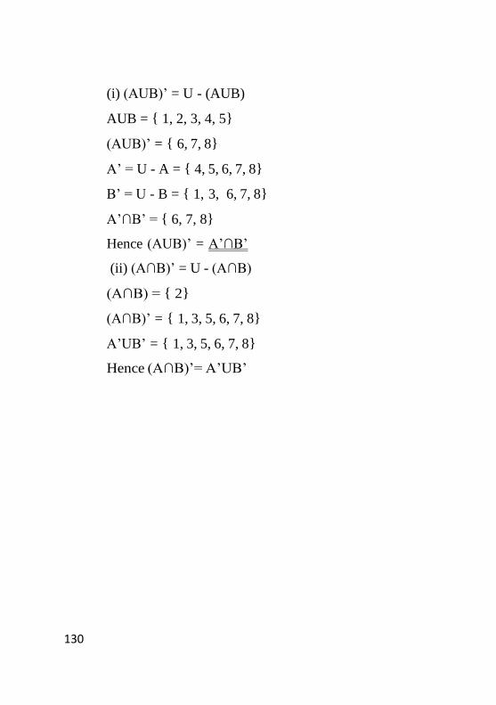
130
(i) (AUB)’ = U - (AUB)
AUB = { 1, 2, 3, 4, 5}
(AUB)’ = { 6, 7, 8}
A’ = U - A = { 4, 5, 6, 7, 8}
B’ = U - B = { 1, 3, 6, 7, 8}
A’∩B’ = { 6, 7, 8}
Hence (AUB)’ = A’∩B’
(ii) (A∩B)’ = U - (A∩B)
(A∩B) = { 2}
(A∩B)’ = { 1, 3, 5, 6, 7, 8}
A’UB’ = { 1, 3, 5, 6, 7, 8}
Hence (A∩B)’= A’UB’

131
Venn Diagram
The relationship between sets can be represented by means of
diagrams. It is known as Venn diagram. It consists of a
rectangle and circles. Rectangle represents the universal set and
circle represents any set.
For example AUB, A∩B, A-B, and ACcan be represented as
follows:
1. AUB 1 2
3
In the first diagram A and B are intersecting in the second
diagram, A and B are disjoint and in the third figure, B is a
subset of A. In all the diagrams, AUB is equal to the shaded
area.
A B B A
A
A
B

132
2. A∩B
1 2
3
In first diagram A∩B is marked by lines. In the second diagram
A and B are disjoint and therefore there is no intersection and
so A∩B = Ø. In the third diagram B is a subset of A and A∩B
is also marked by lines.
3. A-B
A B B A
A
B
A B

133
A – B ie belongs to A but not in B is shaded by lines
4. Ac
Ac i.e. belongs to universe but not in A is shaded by lines
Theorems on Number of Elements in a Set.
(i)n(AUB) = n(A) + n(B) – n(A∩B)
(ii) n(AUBUC) = n(A) + n(B) + n(C) – n(A∩B) – n(A∩C) –
n(B∩C) + n(A∩B∩C)
AUB = at least one of them
A∩B = both A & B
AUBUC = At least one of them
A∩B∩C = All of them
1. Among 60 people, 35 can speak in English, 40 in Malayalam
and 20 can speak in both the languages. Find the number of
people who can speak at least one of the languages. How many
cannot speak in any of these languages?
A

134
Solution
n(A) = Speak in English
n(B) = Speak in Malayalam
Given
n(A) = 35, n(B) = 40
n(A∩B) = 20
AUB = (ie people who speak in at least one of the language)
= n(A) + n(B) – n(A∩B)
= 35 + 40 - 20 = 55
Number of people who cannot speak in any one of these
language = 60- 55 = 5
2. Each student in a class, studies at least one of the subject
English, Mathematics and Accountancy. 16 study English, 22
Accountancy and 26 Mathematics. 5 study English and
Accountancy, 14 study Mathematics and Accountancy and 2
English, Accountancy and Mathematics. Find the number of
student who study
i. English & Mathematics
ii. English, Mathematics but not Accountancy
Solution
Let A = students study English
B = students study Mathematics

135
C = students study Accountancy
Given
n(A ) = 16, n(B) 26, n(C) 22
n(A∩C) = 5, n (B∩C) = 14, n(A∩B)?
n(A∩B∩C) = 2, n(AUBUC) = 40
We know that
n(AUBUC) = n(A) + n(B) + n(C) – n(A∩B) –n(A∩C) –n(B∩C)
+ n(A∩B∩C)
40 = 16 + 26 + 22 - n(A∩B) – 5 – 14 + 12
n(A∩B) = 16 + 26 + 22 – 5 – 14 + 2 – 40
= 7
Number of students study for English & Mathematics = 7∴
Number of student who study English, Mathematics but not
Accountancy= n(A∩B∩C’) n(A∩B∩C’) = n(A∩B)-n(A∩B∩C)
= 7 – 2 = 5
Number of student who study English, Mathematics and not
Accountancy = 5
3. In a college there are 20 teachers, who teach Accountancy or
Statistics. Of these 12, teach Accountancy and 4 teach both
Statistics and Accountancy. How many teach Statistics?
Solution
Let n(A) = teachers teach Accountancy

136
n(B) = teacher teach Statistics
Given
n(A) = 12, n(B) ?
n(A∩B) = 4, n(AUB) =20
n(AUB) = n(A) + n(B) - n(A∩B)
20 = 12 + n(B) – 4
n(B) = 20 – 12 + 4 = 12
Number of teachers teach Statistics = 12
4. Out of 2400 students who appeared for BCom degree
Examination, 1500 failed in Numerical skills, 1200 failed in
Accountancy and 1200 failed in Informatics, 900 failed in both
Numerical skills and Accountancy 800 failed in both
Numerical skills and Informatics, 300 failed in Accountancy
and Informatics, 40 failed in all subjects. How many students
passed all three subjects?
Solution
Let A = number of students failed in Numerical Skills
B = number of students failed in Accountancy
C = number of students failed in Informatics
Given
n(A) = 1500, n(B) = 1200, n(C) = 1200
n(A∩B) = 900, n(A∩C)= 800, n(B∩C) = 300

137
n(A∩B∩C) = 40
Number of st udents failed in at least one subject
= n(AUBUC) n(AUBUC) = n(A) + n(B) + n(C) - n(A∩B) -
n(A∩C)‐ n(B∩C) + n(A∩B∩C)
= 1500 + 1200 + 1200 – 900 – 800 – 300 + 40 = 1940
Number of student passed in all subjects = 2400 – 1940 = 460

138
Module V: Theoretical Distribution
Probability distribution (Theoretical Distribution) can be defined as a
distribution obtained for a random variable on the basis of a
mathematical model. It is obtained not on the basis of actual
observation or experiments, but on the basis of probability law.
Random variable
Random variable is a variable who value is determined by the
outcome of a random experiment. Random variable is also called
chance variable or stochastic variable.
For example, suppose we toss a coin. Obtaining of head in this
random experiment is a random variable. Here the random variable
of “obtaining heads” can take the numerical values.
Now, we can prepare a table showing the values of the random
variable and corresponding probabilities. This is called probability
distributions or theoretical distribution. In the above, example
probability distribution is :-
Obtaining of heads X Probability of obtaining heads P(X)
0
1
1
2
1
2

139
∑P(X) = 1
Properties of Probability Distributions:
Every value of probability of random variable will be greater than or
equal to zero. i.e., P(X) 0
i.e., P(X) Negative value
Sum of all the probability values will be 1
∑P(X) = 1
Question
A distribution is given below. State whether this distribution is a
probability distribution.
X: 0 1 2 3 4
P(X): 0.01 0.10 0.50 0.30 0.90
Solution
Here all values of P(X) are more that zero; and sum of all P(X)
value is equal to 1
Since two conditions, namely P(X) 0 and ∑P(X) = 1, are satisfied,
the given distribution is a probability distribution.
Mathematical Expectation
(Expected Value)

140
If X is a random variable assuming values x1, x2 , x3 ,…………, xn
with corresponding probabilities P1 , P2 , P3 ,…………, Pn, then the
operation of X is defined as X1P1 + X2 P2 + X3 P3 ……… Xn Pn
E(X) = ∑[X.P(X)]
Question
A petrol pump proprietor sells on an average Rs. 80,000/- worth of
petrol on rainy days and an average of Rs. 95.000 on clear days.
Statistics from the meteorological department show that the
probability is 0.76 for clear weather and 0.24 for rainy weather on
coming Wednesday. Find the expected value of petrol sale on
coming Wednesday.
Expected Value E(X) = ∑ [X.P(X)]
= (80000× 0.24) + (95000× 0.76)
= 19200+72.200
= Rs.91400
Question
There are three alternative proposals before a business man to start
a new project:-
Proposal I: Profit of Rs. 5 lakhs with a probability of 0.6 or a
loss of Rs. 80,000 with a probability of 0.4.
Proposal II: Profit of Rs. 10 laksh with a probability of 0.4 or a loss
of Rs. 2 lakhs with a probability of 0.6

141
Proposal III: Profit of Rs. 4.5 lakhs with a probability of 0.8 or a loss
of Rs. 50,000 with a probability of 0.2
If he wants to maximize profit and minimize the loss, which
proposal he should prefer?
Solution
Here, we should calculate the mathematical expectation of each
proposal.
Expected Value E(X) = ∑ [X.P(X)]
Expected value of Proposal I
= (5,00.000 × 0.6) +(80.000 × 0.4)
= 300,000 – 32,000
= Rs.2, 68,000
Expected value of Proposal II
= (10,00.000 × 0.4) +(-2,00.000 × 0.6)
= 4,00.000 – 1,20.000
= 2,80,000.
Expected value of Proposal III
= (4,50,000 × 0.8) +(-50,000 × 0.2)
= 3,60,000 – 10,000
= 3,50,000
Since expected value is highest in case of proposal III, the
businessman should prefer the proposal III
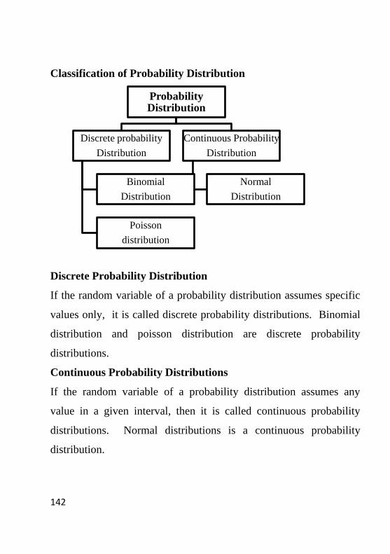
142
Classification of Probability Distribution
Discrete Probability Distribution
If the random variable of a probability distribution assumes specific
values only, it is called discrete probability distributions. Binomial
distribution and poisson distribution are discrete probability
distributions.
Continuous Probability Distributions
If the random variable of a probability distribution assumes any
value in a given interval, then it is called continuous probability
distributions. Normal distributions is a continuous probability
distribution.
Probability Distribution
Discrete probability
Distribution
Binomial
Distribution
Poisson
distribution
Continuous Probability
Distribution
Normal
Distribution

143
Bionomial Distribution
Meaning & Definition:
Binomial Distribution is associated with James Bernoulli, a Swiss
Mathematician. Therefore, it is also called Bernoulli distribution.
Binomial distribution is the probability distribution expressing the
probability of one set of dichotomous alternatives, i.e., success or
failure. In other words, it is used to determine the probability of
success in experiments on which there are only two mutually
exclusive outcomes. Binomial distribution is discrete probability
distribution.
Binomial Distribution can be defined as follows: “A random
variable r is said to follow Binomial Distribution with parameters n
and p if its probability function is:
P(r) = nCrprqn-r
Where, P = probability of success in a single trial
q = 1 – p
n = number of trials
r = number of success in ‘n’ trials.
Assumption of Binomial Didstribution OR
(Situations where Binomial Distribution can be applied)
Binomial distribution can be applied when:-
144
1. The random experiment has two outcomes i.e., success and
failure.
2. The probability of success in a single trial remains constant
from trial to trial of the experiment.
3. The experiment is repeated for finite number of times.
4. The trials are independent.
Properties (features) of Binomial Distribution
1. It is a discrete probability distribution.
2. The shape and location of Binomial distribution changes as
‘p’ changes for a given ‘n’.
3. The mode of the Binomial distribution is equal to the value
of ‘r’ which has the largest probability.
4. Mean of the Binomial distribution increases as ‘n’ increases
with ‘p’ remaining constant.
5. The mean of Binomial distribution is np.
6. The Standard deviation of Binomial distribution is √𝑛𝑝𝑞
7. If ‘n’ is large and if neither ‘p’ nor ‘q’ is too close zero,
Binomial distribution may be approximated to Normal
Distribution.
8. If two independent random variables follow Binomial
distribution, their sum also follows Binomial distribution.

145
Qn: Six coins are tossed simultaneously. What is the probability of
obtaining 4 heads?
Sol: P(r) = nC r prqn-r
r = 4
n = 6
p = ½
q = 1 – p = 1 – ½ = ½
∴ p( r = 4) = 6C4 ( ½ )4 ( ½ )6-4
=6!
(6−4)!4!! x (½)4+2
= 6!
2!4!! x (½)6
= 6×5
2×1 x
1
64
= 30
128
= 0.234
Qn: The probability that Sachin Tendulkar scores a century in a
cricket match is1
3. What is the probability that out of 5 matches, he
may score century in: -
(1) Exactly 2 matches
(2) No match
Sol: Here p = 1
3

146
q = 1 - 1
3=
2
3
P(r) = nC r prqn-r
Probability that Sachin scores centuary in exactly 2 matches is:
p (r = 2) = 5 C2 (1
3)2 (
2
3)2
= 5!
(5−2)!2! x
1
9 ×
8
27
= 5×4
2×1×
1
279×
8
27
= 160
486
= 80
243
= 0.329
Probability that Sachin scores centuary in no matches is:
p (r = 0) = 5 C0 (1
3)0 (
2
3)5−0
= 5!
(5−0)!0! x1 × (
2
3)5
= 5!
2!×0!× 1
32
243
= 32
243
= 0.132
Mean and Standard Deviation of Binomial Distribution
Mean of Binomial Distribution = np
Standard Deviation of Binomial Distribution =√𝑛𝑝𝑞

147
Qn: For a Binomial Distribution, mean = 4 and variance = 12
9 . Find
n.
Sol: Mean = np = 4
Standard Deviation = √𝑛𝑝𝑞
∴ Variance = Standard Deviation 2
=( √𝑛 𝑝𝑞)2
= npq
npq = 12
9
Divide npq by np to get the value of q
i.e. = 𝑛𝑝𝑞
𝑛𝑝= 𝑞
q = 𝑛𝑝𝑞
𝑛𝑝 =
12
94
1
= 12
9 ×
1
4
= 3
9=
1
3
q = 1
3
p = 1 – q
= 1 – 1
3 =
2
3
np = 4
n× 2
3 = 4
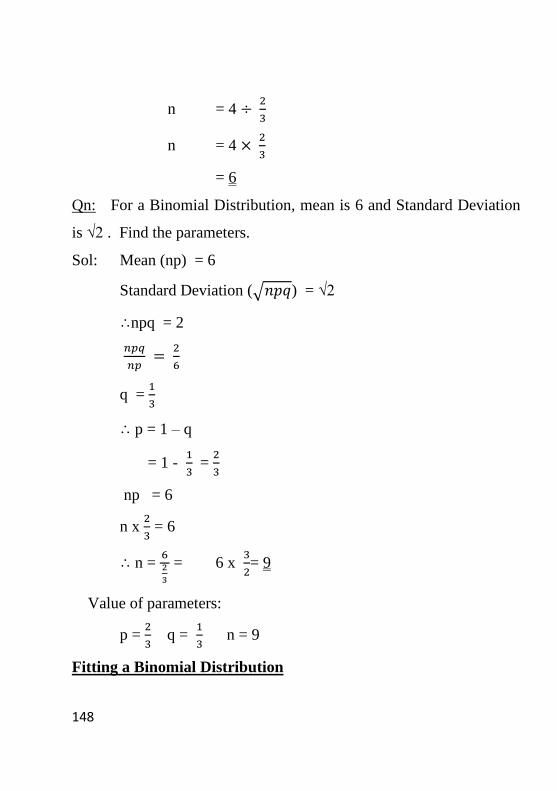
148
n = 4 ÷ 2
3
n = 4 × 2
3
= 6
Qn: For a Binomial Distribution, mean is 6 and Standard Deviation
is √2 . Find the parameters.
Sol: Mean (np) = 6
Standard Deviation (√𝑛𝑝𝑞) = √2
∴npq = 2
𝑛𝑝𝑞
𝑛𝑝 =
2
6
q = 1
3
∴ p = 1 – q
= 1 - 1
3 =
2
3
np = 6
n x 2
3 = 6
∴ n = 62
3
= 6 x 3
2= 9
Value of parameters:
p = 2
3 q =
1
3 n = 9
Fitting a Binomial Distribution

149
Steps:
Find the value of n, p and q
Substitute the values of n, p and q in the Binomial Distribution
function of nCrprqn-r
Put r = 0, 1, 2, ……….. in the function nCrprqn-r
Multiply each such terms by total frequency (N) to obtain the
expected frequency.
Qn: Eight coins were tossed together for 256 times. Fit a Binomial
Distribution of getting heads. Also find mean and standard
deviation.
Sol: p (getting head) = p = 1
2
q = 1 -1
2 =
1
2
n = 8
Binomial Distribution function is p(r) = nCrprqn-r
Put r= 0, 1, 2, 3 …….. 8, then are get the terms of the
Binomial Distribution.
No. of
heads
i.e. r
P (r)
Expected
Frequency
P (r) x N
N = 256
0 8 C0 (1
2)0 (
1
2)8 = 1× 1 ×
1
256=
1
256 1

150
1 8 C1 (1
2)1 (
1
2)7 = 8 ×
1
256=
8
256 8
2 8 C2 (1
2)2 (
1
2)6 = 28 ×
1
256=
28
256 28
3 8 C3 (1
2)3 (
1
2)5 = 56 ×
1
256=
56
256 56
4 8 C4 (1
2)4 (
1
2)4 = 70 ×
1
256=
70
256 70
5 8 C5 (1
2)5 (
1
2)3 = 56 ×
1
256=
56
256 56
6 8 C6 (1
2)6 (
1
2)2 = 28 ×
1
256=
28
256 28
7 8 C7 (1
2)7 (
1
2)1 = 8 ×
1
256=
8
256 8
8 8 C8 (1
2)8 (
1
2)0 = 1 ×
1
256=
1
256 1
Mean = np
= 8×1
2 = 4
Standard Deviation = (√𝑛𝑝𝑞)
=√8 × 1
2×
1
2
= √2 = 1.4142
151
Poisson Distribution
Meaning and Definition:
Poisson Distribution is a limiting form of Binomial Distribution.
In Binomial Distribution, the total numbers of trials are known
previously. But in certain real life situations, it may be impossible
to count the total number of times a particular event occurs or does
not occur. In such cases Poisson Distribution is more suitable.
Poison Distribution is a discrete probability distribution. It was
originated by Simeon Denis Poisson.
The Poisson Distribution is defined as:-
p (r) = 𝑒−𝑚 𝑚𝑟
𝑟! .
Where r = random variable (i.e., number of success in ‘n’ trials.
e = 2.7183
m = mean of poisson distribution
Properties of Poisson Distribution
1. Poisson Distribution is a discrete probability distribution.
2. Poisson Distribution has a single parameter ‘m’. When ‘m’
is known all the terms can be found out.
3. It is a positively skewed distribution.
4. Mean and Varriance of Poisson Distribution are equal to
‘m’.
152
5. In Poisson Distribution, the number of success is relatively
small.
6. The standard deviation of Poisson Distribution is √m.
Practical situations where Poisson Distribution can be used
1. To count the number of telephone calls arising at a
telephone switch board in a unit of time.
2. To count the number of customers arising at the super
market in a unit of time.
3. To count the number of defects in Statistical Quality
Control.
4. To count the number of bacterias per unit.
5. To count the number of defectives in a park of manufactured
goods.
6. To count the number of persons dying due to heart attack in
a year.
7. To count the number of accidents taking place in a day on a
busy road.
Qn: A fruit seller, from his past experience, knows that 3% of
apples in each basket will be defectives. What is the probability
that exactly 4 apples will be defective in a given basket?
Sol: p (r) = 𝑒−𝑚 𝑚𝑟
𝑟!
153
m = 3
. .
∴p (r = 4) = 𝑒−−3 . 34
4! =
0.04979×81
4×3×2×1
= 0.04979×81
24
= 0.16804
Qn: It is known from the past experience that in a certain plant,
there are on an average four industrial accidents per year.
Find the probability that in a given year there will be less
than four accidents. Assume poisson distribution.
Sol: p (r<4) = p(r = 0 or 1 or 2 or 3)
= p (r = 0) + p (r =1) + p (r = 2) + p (r = 3)
P (r) = 𝑒−𝑚 𝑚𝑟
𝑟!
m = 4
∴p (r = 0) = 𝑒−4 . 40
0! =
0.01832×1
1= 0.01832
p (r =1) = 𝑒−4 . 41
1! =
0.01832×4
1= 0.07328
p (r = 2) = 𝑒−4 . 42
2! =
0.01832×16
2×1= 0.14656
p (r = 3) = 𝑒−4 . 43
3! =
0.01832×64
3×2×1= 0.19541
∴p (r < 4) = 0.01832 + 0.07328 + 0.14656 + 0.19541
154
= 0.43357
Qn: Out of 500 items selected for inspection, 0.2% are found to be
defective. Find how many lots will contain exactly no defective if
there are 1000 lots.
Sol: p = 0.2% = 0.002
n= 500
m = np = 500 x 0.002 = 1
P (r) = 𝑒−𝑚 𝑚𝑟
𝑟!
P (r = 0) = 𝑒−1 . 10
0! =
0.36788 ×1
1= 0.36788
∴ Number of lots containing no defectives if there are 1000 lots
= 0.36788 x 1000
= 367.88
= 368
Qn: In a factory manufacturing optical lenses, there is a small
chance of 1
1500 for any one lense to be defective. The lenses are
supplied in packets of 10. Use Poisson Distribution to
calculate the approximate number of packets containing (1) one
defective (2) no defective in a consignment of 20,000 packets. You
are given that e-0.02 = 0.9802.
Sol: n = 10

155
p = probability of manufacturing defective lense= 1
500 = 0.002
m = np = 10 x 0.002 = 0.02
p (r) = 𝑒−𝑚 𝑚𝑟
𝑟!
p (r = 1) = 𝑒−0.02 0.021
1! =
0.9802 ×0.02
1= 0.019604
∴ No. of packets containing one defective lense
=0.019604 x 20,000
= 392
p (r = 0) = 𝑒−0.02 0.020
0! =
0.9802 ×1
0
= 0.9802
∴ No. of packets containing no defective lense = 0.9892 x 20,000
= 19604
Qn: A Systematic sample of 100 pages was taken from a
dictionary and the observed frequency distribution of foreign
words per page was found to be as follows:
No. of foreign words per page (x) : 0 1 2 3 4 5 6
Frequency (f) : 48 27 12 7 4 1 1
Calculate the expected frequencies using Poisson Distribution.
Sol: p (r) = 𝑒−𝑚 𝑚𝑟
𝑟!
Here first we have to find out ‘m’

156
Computation of mean (m)
x f fx
0 48 0
1 27 27
2 12 24
3 7 21
4 4 16
5 1 5
6 1 6
N = 100 Σfx = 99
�̅� = ∑𝑓𝑥
𝑁 =
99
100 = 0.99
∴ m = 0.99
∴ Poisson Distribution = 𝑒−0.99 . (0.99)𝑟
𝑟!
Computation of expected frequencies
x p (x) Expected frequency Nx p(x)

157
0 𝑒−0.99 . (0.99)0
0!= 0.3716 100 x 0.3716 = 37.2
1
𝑒−0.99 . (0.99)1
1! = 0.3679
100 x 0.3679 = 36.8
2 𝑒−0.99 . (0.99)2
2! = 0.1821
100 x 0.1821 = 18.21
3 𝑒−0.99 . (0.99)3
3!= 0.0601 100 x 0.0601 = 6
4 𝑒−0.99 . (0.99)4
4!= 0.0149 100 x 0.0149 = 1.5
5 𝑒−0.99 . (0.99)5
5!= 0.0029 100 x 0.0029 = 0.3
6 𝑒−0.99 . (0.99)6
6! = 0.0005 100 x 0.0005 = 0.1
Hence, the expected frequencies of this Poisson Distribution are:-
No. of foreign words per
page : 0 1 2 3 4 5 6
Expected frequencies
(Rounded): 37 37 18 6 2 0 0

158
Normal Distribution
The normal distribution is a continuous probability distribution. It
was first developed by De-Moivre in 1733 as limiting form of
binomial distribution. Fundamental importance of normal
distribution is that many populations seem to follow approximately a
pattern of distribution as described by normal distribution.
Numerous phenomena such as the age distribution of any species,
height of adult persons, intelligent test scores of students, etc. are
considered to be normally distributed.
Definition of Normal Distribution
A continuous random variable ‘X’ is said to follow Normal
Distribution if its probability function is:
P (X) = 1
√2𝜋𝜎× 𝑒
1
2 (
𝑥− 𝜇
𝜎)2
π = 3.146
e = 2.71828
µ = mean of the distribution
σ = standard deviation of the distribution
Properties of Normal Distribution (Normal Curve)
1. Normal distribution is a continuous distribution.
2. Normal curve is symmetrical about the mean.
3. Both sides of normal curve coincide exactly.
159
4. Normal curve is a bell shaped curve.
5. Mean, Median and Mode coincide at the centre of the curve.
6. Quantities are equi-distant from median.
Q3 – Q2 = Q2 – Q1
7. Normal curve is asymptotic to the base line.
8. Total area under a normal curve is 100%.
9. The ordinate at the mean divide the whole area under a
normal curve into two equal parts.
(50% on either side).
10. The height of normal curve is at its maximum at the mean.
11. The normal curve is unimodel, i.e., it has only one mode.
12. Normal curve is mesokurtic.
13. No portion of normal curve lies below the x-axis.
14. Theoretically, the range of normal curve is – α to + α .
But practically the range is µ - 3σ to µ + 3σ.
µ ± 1σ covers 68.27% area
µ ± 2σ covers 95.45% area
µ ± 3σ covers 98.73% area.
Importance (or uses) of Normal Distribution
The normal distribution is of central importance in statistical
analysis because of the following reasons:-

160
1. The discrete probability distributions such as Binomial
Distribution and Poisson Distribution tend to normal
distribution as ‘n’ becomes large.
2. Almost all sampling distributions conform to the normal
distribution for large values of ‘n’.
3. Many tests of significance are based on the assumption that
the parent population from which samples are drawn follows
normal distribution.
4. The normal distribution has numerous mathematical
properties which make it popular and comparatively easy to
manipulate.
5. Normal distribution finds applications in Statistical Quality
Control.
6. Many distributions in social and economic data are
approximately normal. For example, birth, death, etc. are
normally distributed.
Standard normal probability distribution
A random variable that has a normal distribution with mean ‘0’
and standard deviation 1 is said to have a standard normal
probability distribution.
Z = 𝑋− 𝜇
𝜎

161
Z score can be defined as the number of standard deviation that a
value, x is above or below the mean of the distribution
Using Standard Deviation Units
Because of the equivalence between Z scores and standard
deviation units, probabilities of the normal distribution are often
expressed as ranges of plus-or-minus standard deviation units.
–1σ to +1σ 0.6826
–2σ to +2σ 0.9545
–3σ to +3σ 0.9973
–6σ to +6σ 0.999999998
************************************************