Chapter 4

Quantities and Measurements

I have figured out for you the distance between the horns of a dilemma, night and day, A

and Z. I have computed how far is Up, how long it takes to get Away, and what becomes

of Gone. I have discovered the length of the sea serpent, the price of the priceless, and

the square of the hippopotamus. I know where you are when you are at Sixes and Sevens,

how much Is you have to have to make an Are, and how many birds you can catch with

the salt in the ocean — 187,796,132 if it would interest you to know.

— James Thurber, Many Moons

Consider the following story:

John’s boss kept him at the office one evening, and he got home late. He had promised

his wife that he would get supper ready in time to watch “Dallas,” so he decided to make

hamburgers instead of beef stew. He didn’t have any ground meat in the house, so he

took the car to go to the butcher. The supermarket was closer, but the butcher had

superior meat. On the way, he noticed that he was almost out of gas, so he stopped at

a gas station. When he got to the butcher’s, he saw that the price of ground beef had

gone up again, which the butcher explained was due to the rising price of cattle feed.

John had been getting more and more frustrated, and he yelled at the butcher for being

a thieving scoundrel.

This story has no numbers or mathematics in it. Nonetheless, it is replete with quantities —

parameters which can take greater or lesser values — and it cannot be understood without some

ability to reason about quantities. The quantities in this story include spatial quantities, such as

the distance to the butcher and the supermarket; temporal quantities, such as the times at which

these various events occur, and the length of time needed to cook hamburgers and stew; physical

quantities, such as amount of ground beef and gasoline; psychological quantities, such as the degree

of John’s frustration; economic quantities, such as the price of hamburger; and quantities of other

categories, such as the quality of meat. Some of these quantities are functions of other quantities;

for example, the price of hamburger, the quantity of gasoline, and the distance to the butcher, are

all functions of time. To assert that the gas will run out before the car reaches the butcher requires

comparing the behavior of these two functions.

112

ORD.1. X < Y ⇒¬(Y < X) (Anti-symmetry)

ORD.2. X < Y ∧ Y < Z ⇒ X < Z (Transitivity)

ORD.3. X < Y ∨ Y < X ∨ X = Y (Totality)

Table 4.1: Axioms of Ordering

It is fundamental to mathematics that many aspects of reasoning about quantities are inde-

pendent of the particular domain involved. For that reason, we will study the representations and

reasoning strategies associated with quantities as a whole before entering into their particular ap-

plications. Now, of course, mathematicians have been studying quantities for thousands of years,

and numerical analysts have been studying computations with quantities for hundreds of years, so

we in AI are hardly exploring new ground here. Much of our work has been done for us. Ontolog-

ical issues have been largely settled for us by the work on foundations of mathematics, which has

given solid answers to such questions as, “What is a number?” “What is a function?” “What is an

infinite/infinitesimal quantity?” As regards representations, we have an embarrassment of riches in

the wealth of mathematical symbols and theories which are available. The problem for the AI re-

searcher is largely to determine which mathematical concepts and techniques are appropriate for his

particular application. The common characteristic in AI reasoning about quantities is the focus on

rapidly deriving partial, qualitative conclusions from partial input information, rather than deriving

very detailed and precise information using lengthy calculations.

In this chapter, therefore, rather than systematically review the foundations of arithmetic, we

will consider a series of examples of commonsense quantitative inferences, and examine the repre-

sentations and inferences used in each.

4.1 Order

Examples:

Brown is a better teacher than Crawford. Crawford is a better teacher than Gay. Infer

that Brown is a better teacher than Gay.

Any French wine is classier than any Rhode Island wine. Infer that Rhode Island Red

’83 is not classier than Chateau Lafitte ’23.

The most fundamental quantitative relation is the order relation “X < Y ”. (Note that, in

mathematical parlance, an “inequality” is always an order relation on terms, though there are of

course, many other possible relations besides equality and ordering.) In domains where assigning

exact values is not very meaningful, such as quality of teaching or classiness of wines, order relations

are often the only useful quantitative relations.

Table 4.1 shows the axioms of ordering. A partial ordering obeys axioms ORD.1 and ORD.2; a

total ordering obeys axiom ORD.3 as well.

113

teaching_of teaching_ofteaching_of(Gay) (Crawford) (Brown)

Figure 4.1: Inequalities as a DAG

A logical sort of entity that is partially or totally ordered is called a measure space.1 For example,

“lengths,” “masses,” or “dates” are measure spaces. It makes sense to ask which of two dates is later,

but it makes no sense to ask whether a date is greater than a length. Thus, the relation “X < Y ”,

like most of the quantitative relations we will introduce in this chapter, is polymorphously sorted.

“X < Y ” is meaningful just if X and Y are elements of the same measure space.

A collection of atomic ground inequalities can be implemented as a DAG (directed acyclic graph)

whose nodes are the ground terms and whose arcs correspond to inequalities. In our first exam-

ple above, the nodes would be labelled “teaching of(brown)”, “teaching of(crawford)”, and “teach-

ing of(gay)”, with arcs from Crawford to Brown and from Gay to Crawford. (Figure 4.1.) The

inequality “X < Y ” is a consequence of the input if there is an arc from X to Y in the transi-

tive closure of the DAG. This can be determined in time O(n2) in the worst case, using Dijkstra’s

algorithm.

4.2 Intervals

Example:

The first Crusade occured during the Middle Ages. The Middle Ages predated the

Enlightenment. Infer that the first Crusade predated the Enlightenment.

Many natural entities in commonsense reasoning correspond to intervals of a measure space,

rather than single points. In the above example, the times of the first Crusade, of the Middle Ages,

and of the Enlightenment are intervals of time. In reasoning about the temperature measure space,

it might be natural to pick out the range of comfortable temperatures, the range of temperature in

which water is liquid, and so on.

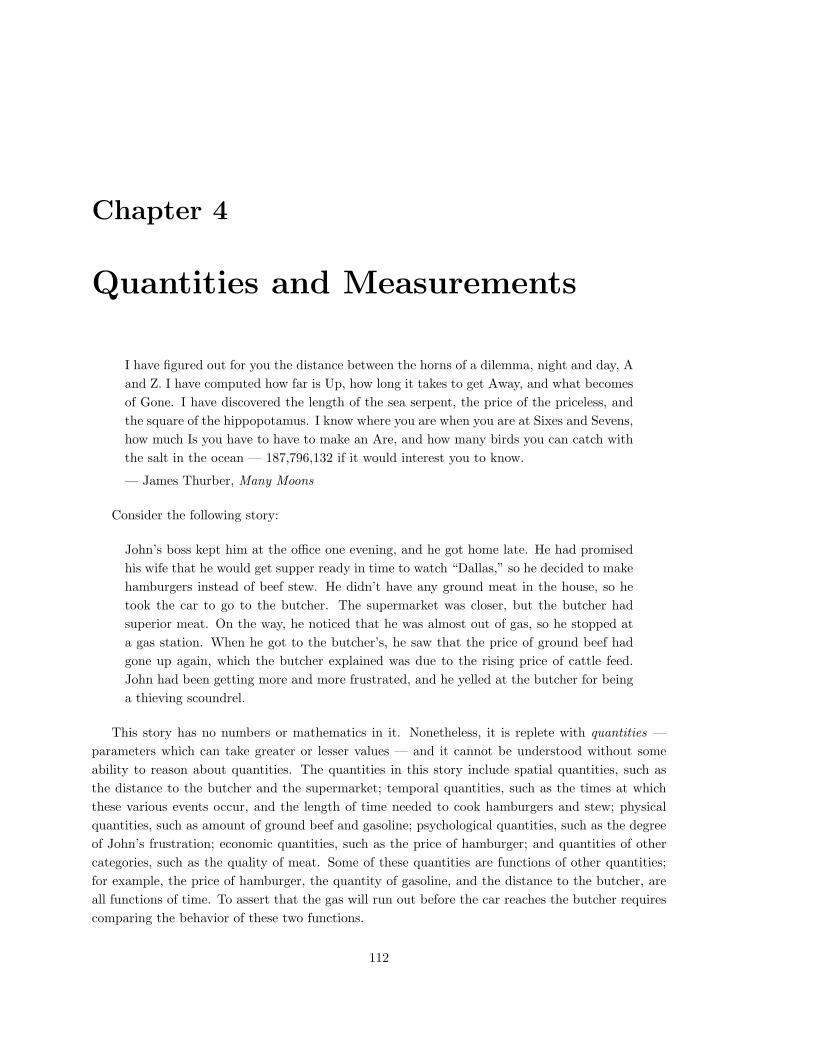
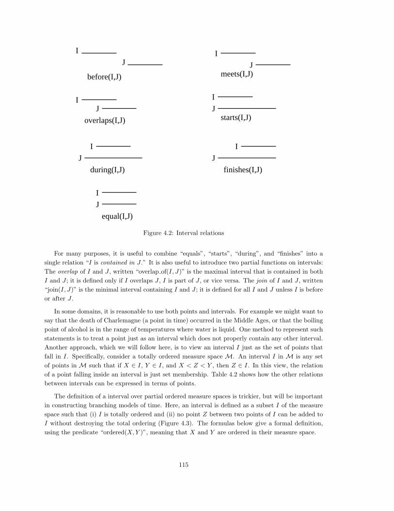
There are thirteen possible order relations between pairs of intervals [Allen, 1983]: Interval I is

before interval J ; I meets J ; I overlaps J ; I starts J ; I finishes J ; I occurs during J ; I is equal to

J ; and the inverses of these (Figure 4.2). (The names of these relations were picked for a temporal

measure space; however, the same basic relations apply to intervals in any measure space.) These

relations can be combined according to rules of transitivity. For instance, the inference in the above

example can be justified by the rule, “If I occurs during J and J precedes K, then I precedes K.”

(See exercise 2 for a discussion of the remaining rules.) It is possible to take as primitive just the

relation “meets(I, J)” and define all the other relations in terms of it. (Table 4.2)

1The term was introduced with this meaning in [Hayes, 1978]. This usage differs from the meaning of “measurespace” in mathematical analysis.

114

I

JI

J

before(I,J)

I

J JI

overlaps(I,J)

I

I

J

J

J

during(I,J)

equal(I,J)

meets(I,J)

starts(I,J)

I

finishes(I,J)

Figure 4.2: Interval relations

For many purposes, it is useful to combine “equals”, “starts”, “during”, and “finishes” into a

single relation “I is contained in J .” It is also useful to introduce two partial functions on intervals:

The overlap of I and J , written “overlap of(I, J)” is the maximal interval that is contained in both

I and J ; it is defined only if I overlaps J , I is part of J , or vice versa. The join of I and J , written

“join(I, J)” is the minimal interval containing I and J ; it is defined for all I and J unless I is before

or after J .

In some domains, it is reasonable to use both points and intervals. For example we might want to

say that the death of Charlemagne (a point in time) occurred in the Middle Ages, or that the boiling

point of alcohol is in the range of temperatures where water is liquid. One method to represent such

statements is to treat a point just as an interval which does not properly contain any other interval.

Another approach, which we will follow here, is to view an interval I just as the set of points that

fall in I. Specifically, consider a totally ordered measure space M. An interval I in M is any set

of points in M such that if X ∈ I, Y ∈ I, and X < Z < Y , then Z ∈ I. In this view, the relation

of a point falling inside an interval is just set membership. Table 4.2 shows how the other relations

between intervals can be expressed in terms of points.

The definition of a interval over partial ordered measure spaces is trickier, but will be important

in constructing branching models of time. Here, an interval is defined as a subset I of the measure

space such that (i) I is totally ordered and (ii) no point Z between two points of I can be added to

I without destroying the total ordering (Figure 4.3). The formulas below give a formal definition,

using the predicate “ordered(X,Y )”, meaning that X and Y are ordered in their measure space.

115

Z

YX

The heavy line shows the interval I.

Figure 4.3: Interval in a Partial Ordering

ordered(X,Y ) ⇔ [ X < Y ∨ Y < X ∨ X = Y ]

interval(I) ⇔

[ [ ∀X,Y ∈I ordered(X,Y ) ] ∧

[ ∀Z 6∈I ∀X,Y ∈I X < Z < Y ⇒∃P∈I ¬ordered(Z,P ) ]]

Another fundamental relation between points and intervals is that a point can be the starting

point or ending point of an interval. We use the function symbols, “start(I)” and “end(I)” to

represent the mappings from an interval to its start and end points. These can be defined as follows:

We define X to be a lower bound of interval I if X is less than or equal to every element of I, and

to be an upper bound of I if X is greater than or equal to every element of I. Then the start of I

is the greatest lower bound for I, if this exists, and the end of I is the least upper bound, if that

exists.

lower bound(X, I) ⇔ ∀Y ∈IY ≥ X

upper bound(X, I) ⇔ ∀Y ∈IY ≤ X

X=start(I) ⇔ lower bound(X, I) ∧ ∀Y lower bound(Y, I) ⇒ Y ≤ X.

X=end(I) ⇔ upper bound(X, I) ∧ ∀Y upper bound(Y, I) ⇒ Y ≥ X.

We can now distinguish four possible behaviors of an interval at each of its ends:

• Interval I is closed below if start(I) exists and is an element of I. I is closed above if end(I)

exists and is an element of I. We use the standard notation ‘[X,Y ]’ to represent the closed

interval from X to Y .

In many applications, it is possible to restrict attention only to closed intervals. In a discrete

measure space, all intervals are closed. In any measure space, closed intervals have the property

that the overlap or join of two closed intervals is a closed interval. However, in order to perform

complementation or set difference in a dense measure space, then it is necessary to go beyond

closed intervals. For example, if the bathroom light is turned on during a time interval that is

closed above, then it must be off during a time interval that is open below. Moreover, in order

to make the standard interval calculus work on a dense interval space containing only closed

116

intervals, it is necessary to disallow closed intervals consisting of a single point, and to define

the relation between interval relations and the points they contain in a somewhat different

way. See table 4.2.

• Interval I is unbounded below if it has no lower bound; it is unbounded above if it has no upper

bound. A theory or algorithm that works correctly for closed intervals can, in many cases, be

adapted to work for unbounded intervals by adding the mythic elements ∞ and −∞ as the

largest and smallest elements of the measure space, and treating an unbounded interval as a

closed interval including these infinite elements. We use the predicates “infinite on right(I)”

and “infinite on left(I)” to characterize intervals that are unbounded above (below).

• Interval I is open (but neither closed or unbounded) below if start(I) exists but is not an

element of I; it is open above if end(I) exists but is not an element of I. The notation ‘(X,Y )’

is standardly used for the open interval from X to Y . In a complete measure space, such as

the real numbers, all intervals are either closed, open, or unbounded in each direction.

• Interval I is gapped below (above) if it has a lower (upper) bound, but no greatest lower

bound (no least upper bound). Such intervals can exists in incomplete spaces. For example,

the set of rational numbers whose square is less than 2 is gapped above, as is also the set of

infinitesimals in a model of the reals with infinitesimals. (See section 4.10). Such intervals do

not have an endpoint, and therefore cannot be denoted in terms of their endpoints; special

purpose representations must be used. (Topologically, such intervals are both closed and open.)

A significant attraction of using just a pure language of intervals and avoiding references to points

is precisely to avoid the hair-splitting issues involved in working out the behavior of the interval at

its endpoint. Even where the structure of the measure space guarantees the existence of an endpoint,

the concept definition may be vague enough to make the endpoints very questionable entities. For

example, if the time line or the temperature scale is taken to have the structure of the real line, then,

provably, every bounded interval has an endpoint. Nonetheless, concepts like “the ending instant

of the Middle Ages,” or “the lower endpoint of the range of comfortable temperatures” are rather

dubious, and one would rather avoid formulating inferences in terms of them.

4.3 Addition and Subtraction

Examples:

On Tuesday night, “Gone with the Wind” and “Duck Soup” are both showing on TV.

“Gone with the Wind” starts later than “Duck Soup” and takes longer. Infer that “Gone

with the Wind” will end later than “Duck Soup”.

Sophy removes a small quantity of flour from a flour bin, and then pours a much larger

quantity into the bin. Infer that there is more flour in the bin at the end than at the

beginning.

The basic concept in these two examples is that of the difference between two quantities, such

as the difference between the ending and starting times of a movie, or the difference between two

117

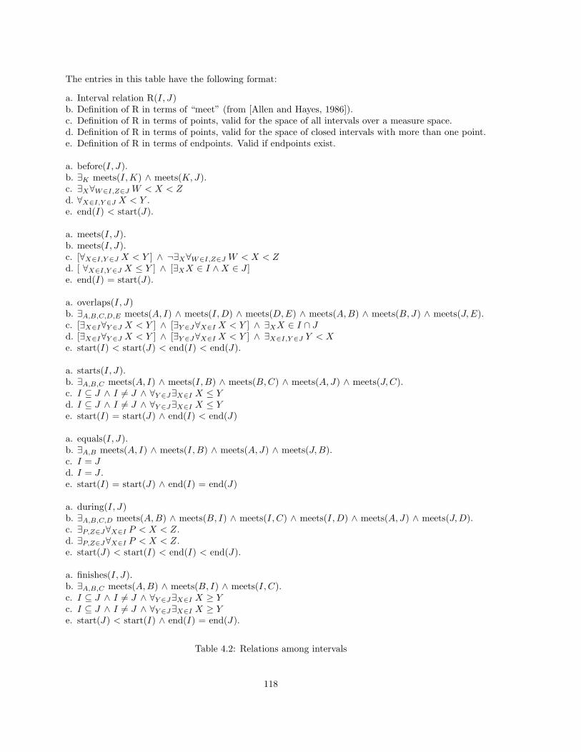
The entries in this table have the following format:

a. Interval relation R(I, J)b. Definition of R in terms of “meet” (from [Allen and Hayes, 1986]).c. Definition of R in terms of points, valid for the space of all intervals over a measure space.d. Definition of R in terms of points, valid for the space of closed intervals with more than one point.e. Definition of R in terms of endpoints. Valid if endpoints exist.

a. before(I, J).b. ∃K meets(I,K) ∧ meets(K,J).c. ∃X∀W∈I,Z∈J W < X < Zd. ∀X∈I,Y ∈J X < Y .e. end(I) < start(J).

a. meets(I, J).b. meets(I, J).c. [∀X∈I,Y ∈J X < Y ] ∧ ¬∃X∀W∈I,Z∈J W < X < Zd. [ ∀X∈I,Y ∈J X ≤ Y ] ∧ [∃XX ∈ I ∧ X ∈ J ]e. end(I) = start(J).

a. overlaps(I, J)b. ∃A,B,C,D,E meets(A, I) ∧ meets(I,D) ∧ meets(D,E) ∧ meets(A,B) ∧ meets(B, J) ∧ meets(J,E).c. [∃X∈I∀Y ∈J X < Y ] ∧ [∃Y ∈J∀X∈I X < Y ] ∧ ∃XX ∈ I ∩ Jd. [∃X∈I∀Y ∈J X < Y ] ∧ [∃Y ∈J∀X∈I X < Y ] ∧ ∃X∈I,Y ∈J Y < Xe. start(I) < start(J) < end(I) < end(J).

a. starts(I, J).b. ∃A,B,C meets(A, I) ∧ meets(I,B) ∧ meets(B,C) ∧ meets(A, J) ∧ meets(J,C).c. I ⊆ J ∧ I 6= J ∧ ∀Y ∈J∃X∈I X ≤ Yd. I ⊆ J ∧ I 6= J ∧ ∀Y ∈J∃X∈I X ≤ Ye. start(I) = start(J) ∧ end(I) < end(J)

a. equals(I, J).b. ∃A,B meets(A, I) ∧ meets(I,B) ∧ meets(A, J) ∧ meets(J,B).c. I = Jd. I = J .e. start(I) = start(J) ∧ end(I) = end(J)

a. during(I, J)b. ∃A,B,C,D meets(A,B) ∧ meets(B, I) ∧ meets(I, C) ∧ meets(I,D) ∧ meets(A, J) ∧ meets(J,D).c. ∃P,Z∈J∀X∈I P < X < Z.d. ∃P,Z∈J∀X∈I P < X < Z.e. start(J) < start(I) < end(I) < end(J).

a. finishes(I, J).b. ∃A,B,C meets(A,B) ∧ meets(B, I) ∧ meets(I, C).c. I ⊆ J ∧ I 6= J ∧ ∀Y ∈J∃X∈I X ≥ Yc. I ⊆ J ∧ I 6= J ∧ ∀Y ∈J∃X∈I X ≥ Ye. start(J) < start(I) ∧ end(I) = end(J).

Table 4.2: Relations among intervals

118

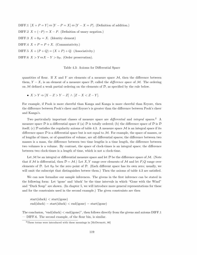
DIFF.1 [X + P = Y ] ⇔ [Y − P = X] ⇔ [Y − X = P ]. (Definition of addition.)

DIFF.2 X + (−P ) = X − P . (Definition of unary negation.)

DIFF.3 X + 0D = X. (Identity element)

DIFF.4 X + P = P + X. (Commutativity.)

DIFF.5 X + (P + Q) = (X + P ) + Q. (Associativity.)

DIFF.6 X > Y ⇔X − Y > 0D. (Order preservation).

Table 4.3: Axioms for Differential Space

quantities of flour. If X and Y are elements of a measure space M, then the difference between

them, Y − X, is an element of a measure space D, called the difference space of M. The ordering

on M defined a weak partial ordering on the elements of D, as specified by the rule below.

• X > Y ⇒ [X − Z > Y − Z] ∧ [Z − X < Z − Y ].

For example, if Pooh is more cheerful than Kanga and Kanga is more cheerful than Eeyore, then

the difference between Pooh’s cheer and Eeyore’s is greater than the difference between Pooh’s cheer

and Kanga’s.

Two particularly important classes of measure space are differential and integral spaces.2 A

measure space D is a differential space if (a) D is totally ordered; (b) the difference space of D is D

itself; (c) D satisfies the regularity axioms of table 4.3. A measure space M is an integral space if its

difference space D is a differential space but is not equal to M. For example, the space of masses, or

of lengths of times, or of quantities of volume, are all differential spaces; the difference between two

masses is a mass, the difference between two time lengths is a time length, the difference between

two volumes is a volume. By contrast, the space of clock-times is an integral space; the difference

between two clock-times is a length of time, which is not a clock-time.

Let M be an integral or differential measure space and let D be the difference space of M. (Note

that if M is differential, then D = M.) Let X,Y range over elements of M and let P,Q range over

elements of D. Let 0D be the zero point of D. (Each different space has its own zero; usually, we

will omit the subscript that distinguishes betwee them.) Then the axioms of table 4.3 are satisfied.

We can now formalize our sample inferences. The givens in the first inference can be stated in

the following form: Let ‘igone’ and ‘iduck’ be the time intervals in which “Gone with the Wind”

and “Duck Soup” are shown. (In chapter 5, we will introduce more general representations for these

and for the constraints used in the second example.) The given constraints are then

start(iduck) < start(igone)

end(iduck) − start(iduck) < end(igone) − start(igone)

The conclusion, “end(iduck) < end(igone)”, then follows directly from the givens and axioms DIFF.1

— DIFF.6. The second example, of the flour bin, is similar.

2These terms were introduced with these meanings in [McDermott, 80]

119

4.4 Real Valued Scales

Example:

Sophy has 8-1/2 pounds of flour in a flour bin. She removes 1/4 pound, and adds 1-3/4

pounds. Infer that Sophy now has 10 pounds of flour in the bin.

In this example, we use numerical values (8-1/2, 1-3/4, 1/4, 10) together with the unit “pound”

to denote different quantities of mass. The legitimacy of doing this, and of basic calculations in a

quantity space on calculations over the reals, is established in the following theorem:

Theorem 4.1: Let D be any differential space satisfying the axioms DIFF.1 — DIFF.6 and also

possessing the Archimedean property:

(Archimedes) For any X,Y > 0 there is an integer N such that Y < X + X + . . . X (N times).

Let U (a unit quantity) be any positive element of D. Then there is a function scaleU (X),

mapping D into the real line, with the following properties:

1. scaleU (U) = 1

2. scaleU (X + Y ) = scaleU (X) + scaleU (Y )

3. X < Y ⇔scaleU (X) < scaleU (Y )

Thus, by fixing a standard unit, such as a pound, we can associate each element of D with a real

number, and we can perform computations on elements of D by performing the same computations

on the corresponding real numbers. (Note that the scale function may map D to some subset of the

reals, such as the integers or the rationals. In that case, it may be possible to use a theory that is

either computationally or ontologically simpler than real arithmetic.)

Similarly, given an integral space M whose difference space has the Archimedean property, it is

possible to choose an arbitrary origin O ∈ M and an arbitrary unit U ∈ D, and then define a scale

in M where O corresponds to 0 and where U corresponds to a difference of 1. For example, the

Centigrade scale associates temperatures with real numbers by choosing the origin to be the freezing

point of water, and the unit to one one-hundredth of the difference between the boiling point and

the freezing point of water.

4.5 More Arithmetic

Examples:

Four quarts of water weigh twice as much as two quarts.

If dinner at Chez Pierre costs more than $50 per person, and there are at least 20 people

in our dinner party, infer that the total bill will be more than $1000.

120

MULT.1 X · Y = Y · X

MULT.2 X · (Y · Z) = (X · Y ) · Z

MULT.3 0 · X = 0

MULT.4 1 · X = X

MULT.5 X > 0 ∧ Y > 0⇒X · Y > 0

Table 4.4: Axioms of Multiplication

The reasoning in these two examples requires introducing some further arithmetic relations.

The first example involves the relation of multiplication. The multiplication function X · Y takes

as arguments two quantities from any two differential quantity spaces, M and N , and returns a

quantity from the product space of M and N . If M is the space of dimensionless quantities (pure

numbers) then the product space of M and N is just N . Table 4.4 shows the well-known axioms of

multiplication.

In axiom MULT.3, the ‘0’ on the left side is the zero point of an arbitrary differential space M;

the ‘0’ on the right is the zero point in the product space of M with the space of X. In axiom

MULT.4, ‘1’ is a dimensionless quantity.

We can now state the general rule that the weight of a quantity of pure stuff is equal to its

volume times the density of the stuff (under standard conditions).

pure(Q,S) ⇒ weight(Q) = volume(Q) · density(S)

Given this physical rule and the above axioms, we can make our desired inference.

[ pure(Q1,water) ∧ pure(Q2,water) ∧

volume(Q1) = 4·quart ∧ volume(Q2) = 2·quart ] ⇒

weight(Q1) = weight(Q2).

The second example requires reasoning about the arithmetic properties of an underspecified

set. To represent this reasoning, we introduce two arithmetic functions over sets. The function

“card(S)” or “|S|” gives the cardinality of a finite set S, which is a dimensionless integer. The

function “sum over(S, F ),” usually written in the form

∑

X∈S

F (X)

gives the sum of function F over the set S. F must be a function mapping S into a differential space

D. Axioms SSUM.1 — SSUM.3 define these functions:

SSUM.1 sum over({X},F ) = F (X)

SSUM.2 A ∩ B = ∅ ⇒ sum over(A ∪ B,F ) = sum over(A,F ) + sum over(B,F ).

121

pan_height

A B pan

spring

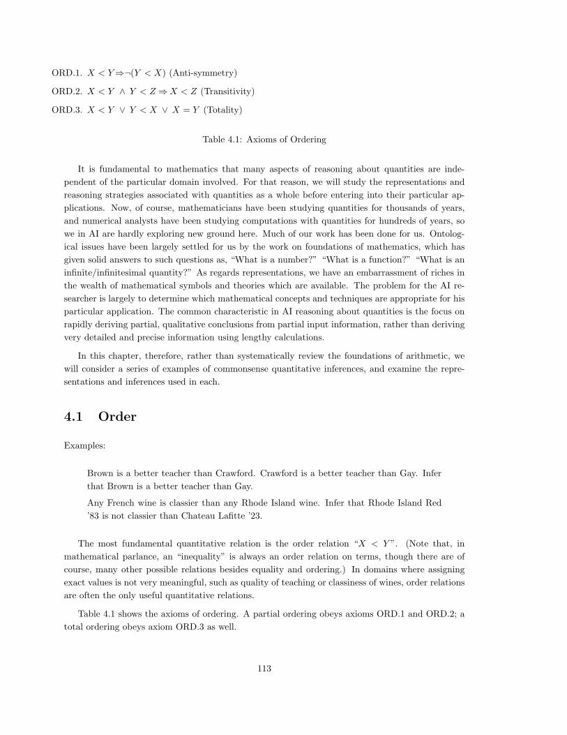
Figure 4.4: Scales

SSUM.3 card(S) = sum over(S,λ(X)(1))

(Note: These axioms involve a second-order logic, which allows quantifying over functions.)

From these axioms, we can deduce the basic result needed for our example: if F (X) > C for

each X ∈ S, then∑

X∈S F is greater than C times the cardinality of S.3

[ ∀X∈S value of(F,X) > C ] ⇒ sum over(S, F ) > C·card(S)

Further arithmetic operators used in spatial reasoning, such as trigonometric functions, will be

introduced in chapter 6.

4.6 Parameters; Signs; Monotonic Relations

Example:

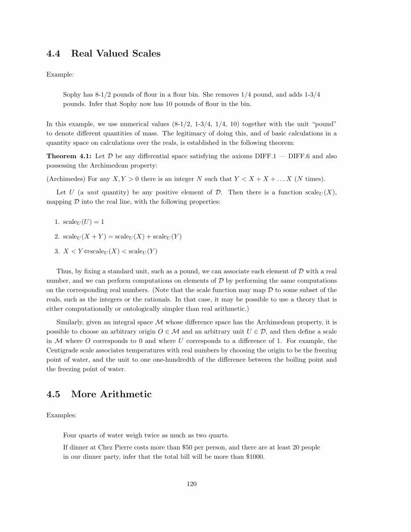
Consider the scales shown in figure 4.4. Suppose that the following constraints are

specified:

• The downward force exerted by each block on the pan is the mass of the block times

the gravitational constant.

• The force exerted by the spring upward on the pan is proportional to the stiffness

of the spring times its compression from its rest length.

• When the scales is at rest, the upward force exerted on the pan by the spring must

exactly balance the sum of the downward forces exerted on the pan by the blocks.

• The height of the pan is equal to the rest length of the spring minus its compression.

Suppose that block A is made more massive, but the scales otherwise remain the same.

Infer that the rest position of the pan is lowered, using the following line of reasoning:

3This proof requires a proof by induction over the cardinality of S, since it applies only to finite sets.

122

Since the mass of A has increased, the force exerted by A must have increased. Since

the mass of B remained the same, the force exerted by B must have remained the same.

Therefore, the sum of the forces exerted by the two blocks must have increased. There-

fore, the upward force exerted by the spring must have increased. Since the stiffness of

the spring has not changed, the compression of the spring must have increased to create

this new force. Since the compression of the spring has increased and its rest length has

remained the same, the pan must be lower.

The form of the inference above is a common one in physical reasoning. We are comparing

situations involving two systems with the same structure but with different values in the input

parameters. We specify the direction of the change between the two situations but not its magnitude.

The problem is to determine, if possible, the direction of change in the output parameters. Note

that we are here only interested in the change in the equilibrium state, when the systems have come

to rest; we are not asking how the system goes from one state to the other. (The dynamic behavior

of this system will be discussed in section 4.9. The problem of deriving the above relations from a

physical description of the system will be discussed in section 7.1.)

The above inference can be expressed and carried out without using any concepts or axioms

beyond those already discussed in previous sections. However, since this type of inference is particu-

larly common in commonsense reasoning about quantities, it is worthwhile developing a specialized

notation and calculation method for dealing with it. In particular, we would like our formal inference

method to resemble the above informal argument in focussing on the increase or decrease in specific

quantities from one situation to the next, and to be able to calculate the direction of change in one

quantity from the direction of change in related quantities.

To do this, we need to be able to refer to a entities such as “the mass of block A” which

may correspond to a particular quantity in each different situation. We therefore introduce the

ontological sort of a parameter. If M is a measure space, then an M-valued parameter is an entity

that associates each situation with a quantity from M; extensionally, the parameter may be viewed

as a function from situations to M. (In chapter 5, we will generalize the concept of a parameter to

that of a general fluent.)

We now introduce a number of functions on parameters. The most basic is the function “value in(S,Q)”,

introduced in section 2.6, which maps a situation S and parameter Q to the value that Q takes in S.

The function delta(Q,S1, S2) gives the change in Q from S1 to S2; it is defined by axiom DEL.1 as

the difference between Q’s values in the two situations. We also introduce arithmetic operations such

as addition, subtraction, multiplication, and so on as operators on parameters. These are defined

by axiom schema DEL.2: the value of the combination of parameters is equal to the combination of

their values.

DEL.1 delta(Q,S1, S2) = value in(S2, Q) − value in(S1, Q).

DEL.2 value in(S, α(Q1, Q2)) = α(value in(S,Q1), value in(S,Q2)) where α is any arithmetic opera-

tor.

We can now express statements like “A increases in mass” in the form “delta(mass(blocka),s1,s2)

> 0.” We can now simplify this form still further. We introduce the function symbol “sign(X),” also

123

written “[X]”, which maps a quantity X onto its sign. We also introduce three constants: “pos”,

the interval of positive quantities; “neg”, the interval of negative quantities; and “ind”, the set of all

quantities. (As with the constant 0, we will use the same symbol to represent these intervals in all

differential spaces.) Thus, if X = 0 then sign(X)=[X] = 0; if X > 0 then [X] =pos; if X < 0 then

[X] =neg. We can then write the above statement in the form, “sign(delta(mass(blocka),s1,s2)) =

pos”. The sign function can be applied to a parameter in the same way as other arithmetic functions;

that is, if Q is a parameter then [Q] is the parameter whose value is always the sign of the value of

the value of Q.

A further notational convenience,4 used in circumstances where we are comparing two fixed

situations s1 and s2, is to abbreviate “sign(delta(Q,s1,s2))” in the form ∆Q. Thus, we can express

the statement “A increases in mass” in the form ∆mass(blockA) = pos. Table 4.5 shows the complete

specification for our example problem.

To carry out inferences from the specifications given in table 4.5, we need rules that will allow

us to start with a parameter equation, such as “weight(blocka) = grav acc · mass(blocka),” combine

this with the values “∆mass(blocka) = pos,” “∆grav acc = 0,” and “[grav acc] = pos,” and to

conclude “∆weight(blocka) = 0.” These rules can be expressed elegantly by splitting them into two

parts.

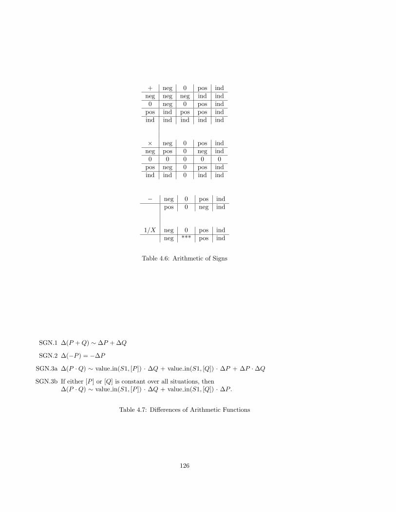
The first part of these inference rules defines the arithmetic operations on the signs pos, 0,

and neg, together with the interval ind (indeterminate), which is the interval of all quantities,

positive, negative, and zero. The arithmetic combination of two signs is all the possible signs of

the combination of values in the signs. For example, pos + pos is pos, because the the sum of any

two positive quantities is positive; pos + neg is ind, because the sum of a positive quantity and a

negative quantity may be positive, zero, or negative, depending on the relative magnitudes of the

two quantities. Table 4.6 shows the arithmetic relations on signs.

Two signs SG1 and SG2 are compatible, written “SG1 ∼ SG2” if there is some quantity in

both.5 Specifically, any sign is compatible with itself, and any sign is compatible with the sign ind.

Note that compatibility is not a transitive relation; ind is compatible with both pos and neg, but

pos is not compatible with neg. Any equation on quantities can be converted into a corresponding

compatibility relation on the signs of the quantities. For example, from the equation X +Y = P ·Q,

it is legitimate to derive the compatibility relation [X]+[Y ] ∼ [P ]·[Q]. (See exercise 4). The converse

is not the case; the truth of a compatibility relation does not imply the truth of the corresponding

equation.

The second part of the inference rules defines the relations among the signs of parameters and

the signs of their changes using the arithmetic on signs. Table 4.7 shows these rules. Combining

these rules, it is straightforward to derive the desired result from the givens of our example of the

scales. Table 4.8 shows the inference path.

The inference in our example that the pan will go down if the weight of A is increased does not,

in fact, depend on the spring obeying the linear law, “spring force = spring · compression.” For the

purposes of this inference, it would be sufficient to know that, for any fixed (positive) value of the

4In the literature, the notation ∂Q is often used for sign(delta(Q,s1,s2)). We will reserve this, however, to meanthe sign of the derivative (see section 4.7).

5In the literature, this is usually written, “SG1 = SG2”; however, this notation is confusing.

124

Constants:

blocka, blockb — Two blocks.s1, s2 — Two situations.

Parameters:

mass(X) — The mass of block X.weight(X) — Downward force exerted by block X.blocks weight — Total downward force exerted by blocks.spring — Stiffness of the spring.compression — Compression of the spring.rest length — Rest length of the spring.spring force — Upward force exerted by spring.pan height — Height of pan.grav acc — Gravitational accelleration.

Constraints:

weight(X) = grav acc · mass(X)blocks weight = weight(blocka) + weight(blockb)spring force = spring · compressionspring force = blocks weightpan height = rest length − compression.

Parameter values:

[spring] = pos[grav acc] = pos

Given Comparisons:

∆mass(blocka) = pos.∆mass(blockb) = 0∆spring = 0.∆rest length = 0.∆grav acc = 0.

Table 4.5: Problem Specification for Scales

125

+ neg 0 pos indneg neg neg ind ind0 neg 0 pos ind

pos ind pos pos indind ind ind ind ind

× neg 0 pos indneg pos 0 neg ind0 0 0 0 0

pos neg 0 pos indind ind 0 ind ind

− neg 0 pos indpos 0 neg ind

1/X neg 0 pos indneg *** pos ind

Table 4.6: Arithmetic of Signs

SGN.1 ∆(P + Q) ∼ ∆P + ∆Q

SGN.2 ∆(−P ) = −∆P

SGN.3a ∆(P · Q) ∼ value in(S1, [P ]) · ∆Q + value in(S1, [Q]) · ∆P + ∆P · ∆Q

SGN.3b If either [P ] or [Q] is constant over all situations, then∆(P · Q) ∼ value in(S1, [P ]) · ∆Q + value in(S1, [Q]) · ∆P .

Table 4.7: Differences of Arithmetic Functions

126

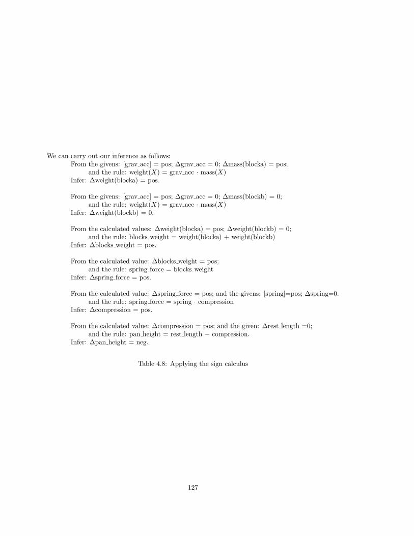
We can carry out our inference as follows:From the givens: [grav acc] = pos; ∆grav acc = 0; ∆mass(blocka) = pos;

and the rule: weight(X) = grav acc · mass(X)Infer: ∆weight(blocka) = pos.

From the givens: [grav acc] = pos; ∆grav acc = 0; ∆mass(blockb) = 0;and the rule: weight(X) = grav acc · mass(X)

Infer: ∆weight(blockb) = 0.

From the calculated values: ∆weight(blocka) = pos; ∆weight(blockb) = 0;and the rule: blocks weight = weight(blocka) + weight(blockb)

Infer: ∆blocks weight = pos.

From the calculated value: ∆blocks weight = pos;and the rule: spring force = blocks weight

Infer: ∆spring force = pos.

From the calculated value: ∆spring force = pos; and the givens: [spring]=pos; ∆spring=0.and the rule: spring force = spring · compression

Infer: ∆compression = pos.

From the calculated value: ∆compression = pos; and the given: ∆rest length =0;and the rule: pan height = rest length − compression.

Infer: ∆pan height = neg.

Table 4.8: Applying the sign calculus

127

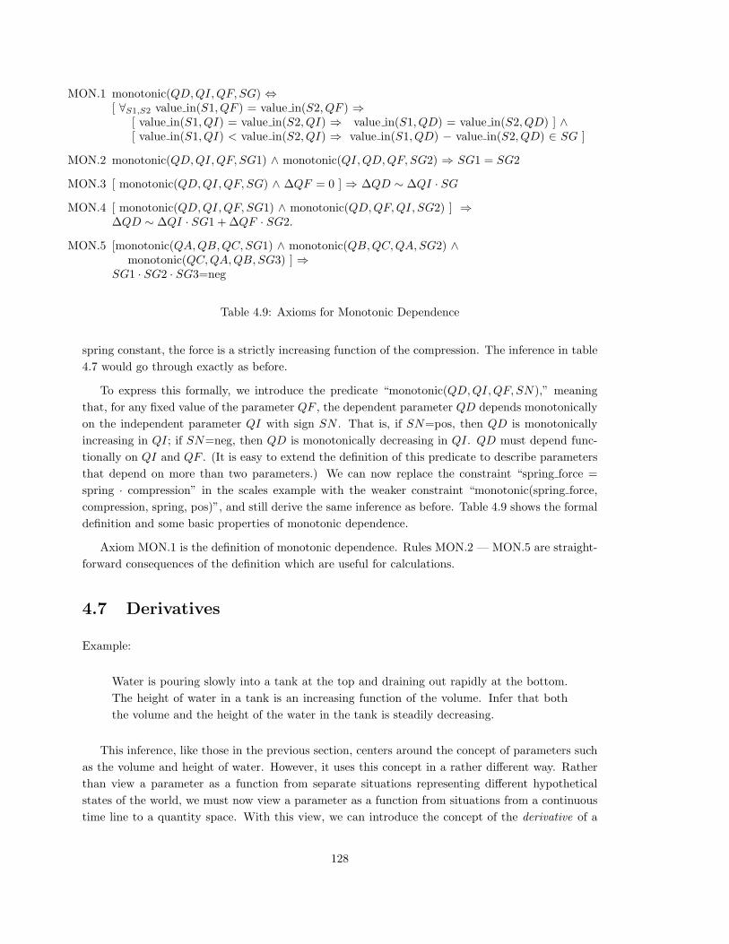
MON.1 monotonic(QD,QI,QF, SG) ⇔[ ∀S1,S2 value in(S1, QF ) = value in(S2, QF ) ⇒

[ value in(S1, QI) = value in(S2, QI) ⇒ value in(S1, QD) = value in(S2, QD) ] ∧[ value in(S1, QI) < value in(S2, QI) ⇒ value in(S1, QD) − value in(S2, QD) ∈ SG ]

MON.2 monotonic(QD,QI,QF, SG1) ∧ monotonic(QI,QD,QF, SG2) ⇒ SG1 = SG2

MON.3 [ monotonic(QD,QI,QF, SG) ∧ ∆QF = 0 ] ⇒ ∆QD ∼ ∆QI · SG

MON.4 [ monotonic(QD,QI,QF, SG1) ∧ monotonic(QD,QF,QI, SG2) ] ⇒∆QD ∼ ∆QI · SG1 + ∆QF · SG2.

MON.5 [monotonic(QA,QB,QC, SG1) ∧ monotonic(QB,QC,QA, SG2) ∧monotonic(QC,QA,QB, SG3) ] ⇒

SG1 · SG2 · SG3=neg

Table 4.9: Axioms for Monotonic Dependence

spring constant, the force is a strictly increasing function of the compression. The inference in table

4.7 would go through exactly as before.

To express this formally, we introduce the predicate “monotonic(QD,QI,QF, SN),” meaning

that, for any fixed value of the parameter QF , the dependent parameter QD depends monotonically

on the independent parameter QI with sign SN . That is, if SN=pos, then QD is monotonically

increasing in QI; if SN=neg, then QD is monotonically decreasing in QI. QD must depend func-

tionally on QI and QF . (It is easy to extend the definition of this predicate to describe parameters

that depend on more than two parameters.) We can now replace the constraint “spring force =

spring · compression” in the scales example with the weaker constraint “monotonic(spring force,

compression, spring, pos)”, and still derive the same inference as before. Table 4.9 shows the formal

definition and some basic properties of monotonic dependence.

Axiom MON.1 is the definition of monotonic dependence. Rules MON.2 — MON.5 are straight-

forward consequences of the definition which are useful for calculations.

4.7 Derivatives

Example:

Water is pouring slowly into a tank at the top and draining out rapidly at the bottom.

The height of water in a tank is an increasing function of the volume. Infer that both

the volume and the height of the water in the tank is steadily decreasing.

This inference, like those in the previous section, centers around the concept of parameters such

as the volume and height of water. However, it uses this concept in a rather different way. Rather

than view a parameter as a function from separate situations representing different hypothetical

states of the world, we must now view a parameter as a function from situations from a continuous

time line to a quantity space. With this view, we can introduce the concept of the derivative of a

128

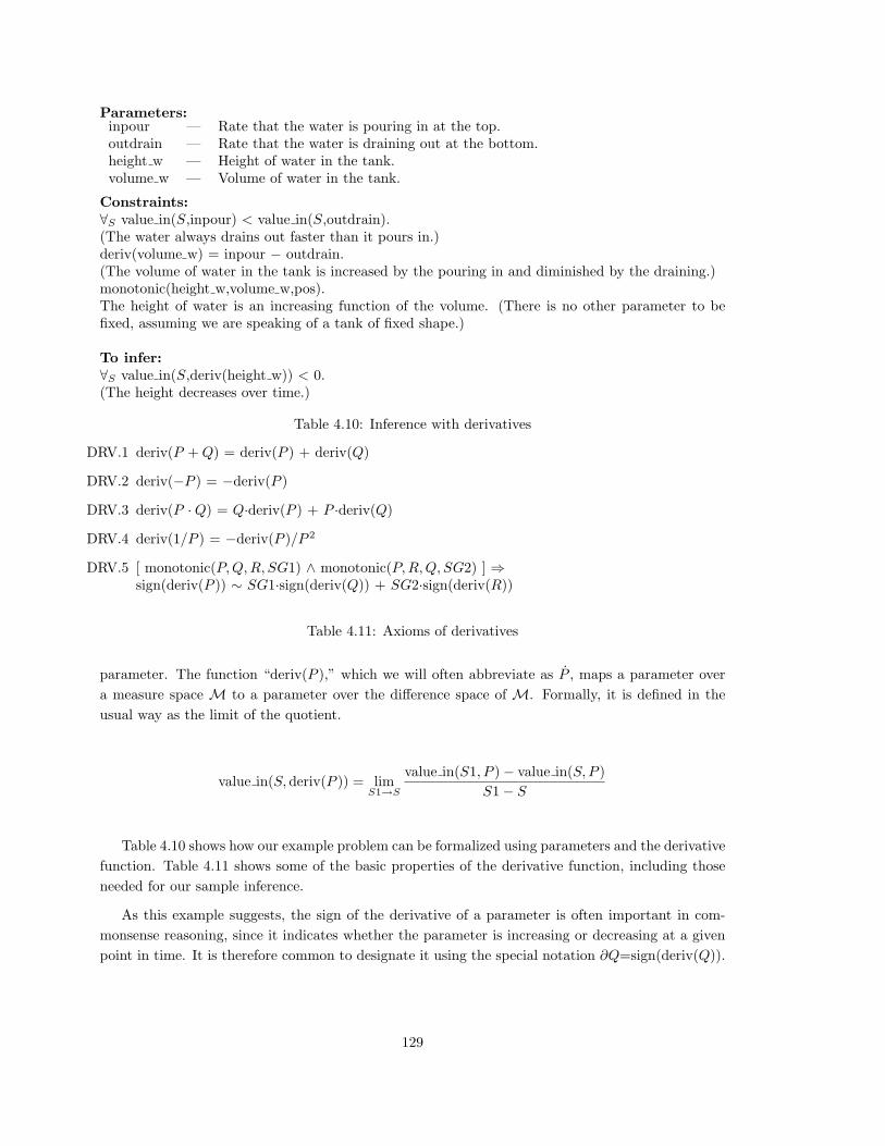
Parameters:inpour — Rate that the water is pouring in at the top.outdrain — Rate that the water is draining out at the bottom.height w — Height of water in the tank.volume w — Volume of water in the tank.

Constraints:

∀S value in(S,inpour) < value in(S,outdrain).(The water always drains out faster than it pours in.)deriv(volume w) = inpour − outdrain.(The volume of water in the tank is increased by the pouring in and diminished by the draining.)monotonic(height w,volume w,pos).The height of water is an increasing function of the volume. (There is no other parameter to befixed, assuming we are speaking of a tank of fixed shape.)

To infer:

∀S value in(S,deriv(height w)) < 0.(The height decreases over time.)

Table 4.10: Inference with derivatives

DRV.1 deriv(P + Q) = deriv(P ) + deriv(Q)

DRV.2 deriv(−P ) = −deriv(P )

DRV.3 deriv(P · Q) = Q·deriv(P ) + P ·deriv(Q)

DRV.4 deriv(1/P ) = −deriv(P )/P 2

DRV.5 [ monotonic(P,Q,R, SG1) ∧ monotonic(P,R,Q, SG2) ] ⇒sign(deriv(P )) ∼ SG1·sign(deriv(Q)) + SG2·sign(deriv(R))

Table 4.11: Axioms of derivatives

parameter. The function “deriv(P ),” which we will often abbreviate as P , maps a parameter over

a measure space M to a parameter over the difference space of M. Formally, it is defined in the

usual way as the limit of the quotient.

value in(S,deriv(P )) = limS1→S

value in(S1, P ) − value in(S, P )

S1 − S

Table 4.10 shows how our example problem can be formalized using parameters and the derivative

function. Table 4.11 shows some of the basic properties of the derivative function, including those

needed for our sample inference.

As this example suggests, the sign of the derivative of a parameter is often important in com-

monsense reasoning, since it indicates whether the parameter is increasing or decreasing at a given

point in time. It is therefore common to designate it using the special notation ∂Q=sign(deriv(Q)).

129

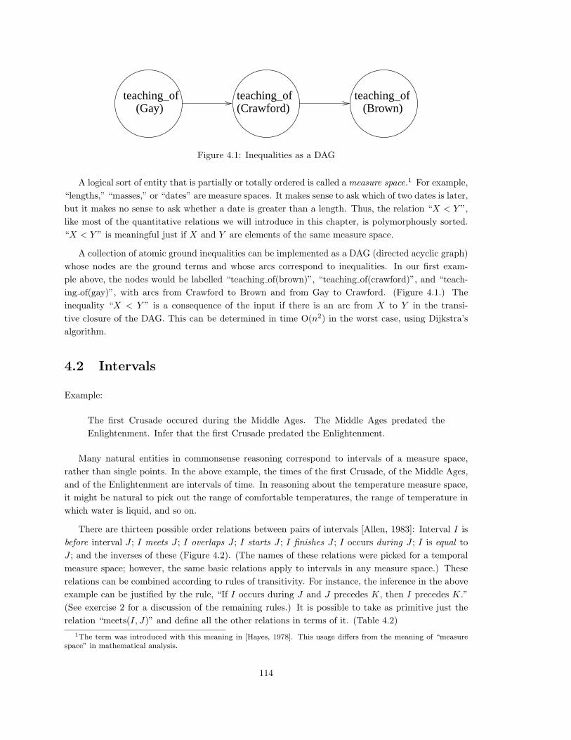
h_both_pend

v_pendv_bot

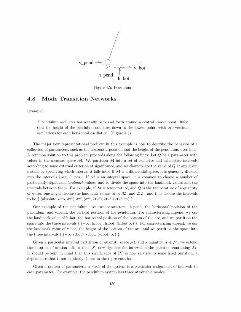
Figure 4.5: Pendulum

4.8 Mode Transition Networks

Example:

A pendulum oscillates horizontally back and forth around a central lowest point. Infer

that the height of the pendulum oscillates down to the lowest point, with two vertical

oscillations for each horizontal oscillation. (Figure 4.5)

The major new representational problem in this example is how to describe the behavior of a

collection of parameters, such as the horizontal position and the height of the pendulum, over time.

A common solution to this problem proceeds along the following lines: Let Q be a parameter with

values in the measure space M. We partition M into a set of exclusive and exhaustive intervals

according to some external criterion of significance, and we characterize the value of Q at any given

instant by specifying which interval it falls into. If M is a differential space, it is generally divided

into the intervals {neg, 0, pos}. If M is an integral space, it is common to choose a number of

particularly significant landmark values, and to divide the space into the landmark values and the

intervals between them. For example, if M is temperature, and Q is the temperature of a quantity

of water, one might choose the landmark values to be 32◦ and 212◦, and thus choose the intervals

to be { (absolute zero, 32◦), 32◦, (32◦, 212◦), 212◦, (212◦,∞) }.

Our example of the pendulum uses two parameters: h pend, the horizontal position of the

pendulum, and v pend, the vertical position of the pendulum. For characterizing h pend, we use

the landmark value of h bot, the horizontal position of the bottom of the arc, and we partition the

space into the three intervals { (−∞, h bot), h bot, (h bot,∞) }. For characterizing v pend, we use

the landmark value of v bot, the height of the bottom of the arc, and we partition the space into

the three intervals { (−∞,v bot), v bot, (v bot, ∞) }

Given a particular interval partitition of quantity space M, and a quantity X ∈ M, we extend

the notation of section 4.6, so that [X] now signifies the interval in the partition containing M.

It should be kept in mind that this significance of [X] is now relative to some fixed partition, a

dependence that is not explicitly shown in the representation.

Given a system of parameters, a mode of the system is a particular assignment of intervals to

each parameter. For example, the pendulum system has three attainable modes:

130

M1

M2

M3

M2

M2M1 M3

Complete and correct network

Correct but incomplete network

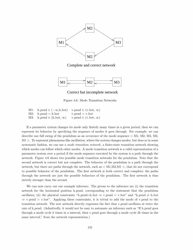
Figure 4.6: Mode Transition Networks

M1: h pend ∈ (−∞,h bot) v pend ∈ (v bot, ∞)M2: h pend = h bot v pend = v botM3: h pend ∈ (h bot, ∞) v pend ∈ (v bot, ∞)

If a parameter system changes its mode only finitely many times in a given period, then we can

represent its behavior by specifying the sequence of modes it goes through. For example, we can

describe one full swing of the pendulum as an occurence of the mode sequence < M1, M2, M3, M2,

M1 >. To represent phenomena like oscillation, where the system changes modes, but does so in some

systematic fashion, we can use a mode transition network , a finite-state transition network showing

which modes can follow which other modes. A mode transition network is a valid representation of a

parameter system over a period if the mode sequence executed by the system is a path through the

network. Figure 4.6 shows two possible mode transition networks for the pendulum. Note that the

second network is correct but not complete. The behavior of the pendulum is a path through the

network, but there are paths through the network, such as < M1,M2,M1 >, that do not correspond

to possible behavior of the pendulum. The first network is both correct and complete; the paths

through the network are just the possible behaviors of the pendulum. The first network is thus

strictly stronger than the second.

We can now carry out our example inference. The givens to the inference are (i) the transition

network for the horizontal position h pend, corresponding to the statement that the pendulum

oscillates; (ii) the physical constraints “h pend=h bot ⇒ v pend = v bot” and “h pend 6= h bot

⇒ v pend > v bot”. Applying these constraints, it is trivial to add the mode of v pend to the

transition network. The new network directly expresses the fact that v pend oscillates at twice the

rate of h pend. (Admittedly, it would not be easy to automate an inference such as “If h pend goes

through a mode cycle k times in a interval, then v pend goes through a mode cycle 2k times in the

same interval,” from the network representation.)

131

Q1 Q2 Q3 Q2 Q1 Q4 Q3 Q4

Q1Q2

Q3 Q4

A curve in the plane

B: Mode sequence

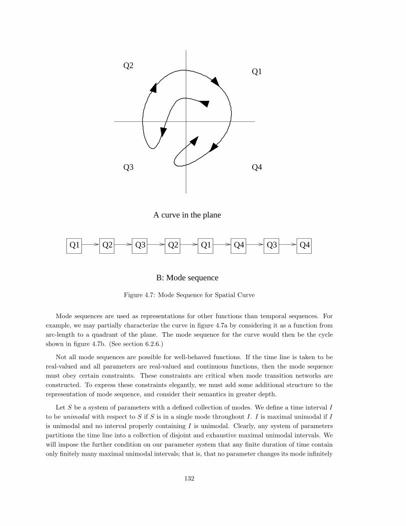
Figure 4.7: Mode Sequence for Spatial Curve

Mode sequences are used as representations for other functions than temporal sequences. For

example, we may partially characterize the curve in figure 4.7a by considering it as a function from

arc-length to a quadrant of the plane. The mode sequence for the curve would then be the cycle

shown in figure 4.7b. (See section 6.2.6.)

Not all mode sequences are possible for well-behaved functions. If the time line is taken to be

real-valued and all parameters are real-valued and continuous functions, then the mode sequence

must obey certain constraints. These constraints are critical when mode transition networks are

constructed. To express these constraints elegantly, we must add some additional structure to the

representation of mode sequence, and consider their semantics in greater depth.

Let S be a system of parameters with a defined collection of modes. We define a time interval I

to be unimodal with respect to S if S is in a single mode throughout I. I is maximal unimodal if I

is unimodal and no interval properly containing I is unimodal. Clearly, any system of parameters

partitions the time line into a collection of disjoint and exhaustive maximal unimodal intervals. We

will impose the further condition on our parameter system that any finite duration of time contain

only finitely many maximal unimodal intervals; that is, that no parameter changes its mode infinitely

132

Let M and N be successive augmented modes in a mode sequence. For any parameter Q let [Q]Mand [Q]N be the modes of Q in M and N . Let IM and IN be the time intervals of M and N .

MODE.1 (Temporal topology) IM is bounded above; IN is bounded below. One of the following twopossibilities must hold:

a. IM is open above and IN is closed below.

b. IM is closed above and IN is open below.

MODE.2 (Change) There is some parameter Q such that [Q]M 6= [Q]N .

MODE.3 (Continuity) For each parameter Q, either [Q]M = [Q]N or the intervals [Q]M and [Q]N areadjacent in the quantity space of Q.

MODE.4 (Parameter topology) If [Q]M 6= [Q]N . then the boundary between [Q]M and [Q]N is topo-logically the same as the boundary between IM and IN . Specifically:

a. If [Q]M < [Q]N , IM is open above, and IN is closed below,then [Q]M is open above and [Q]N is closed below.

b. If [Q]M < [Q]N , IM is closed above, and IN is open below,then [Q]M is closed above and [Q]N is open below.

c. If [Q]M > [Q]N , IM is open above, and IN is closed below,then [Q]M is open below and [Q]N is closed above.

d. If [Q]M > [Q]N , IM is closed above, and IN is open below,then [Q]M is closed below and [Q]N is open above.

MODE.5 Let M , N , and P be three successive augmented modes and Q a parameter such that [Q]Nis closed at both ends and has finite length (not a single point). If [Q]M , [Q]N , and [Q]P allhave different values, then IN has finite length.

Table 4.12: Rules for mode transitions

many times in any finite interval. In this case, the behavior of the system over any finite time interval

may be characterized by a finite mode sequence.

To aid us in stating the restrictions that hold on continuous parameter systems, we augment our

representation of mode sequences. An augmented mode of the parameter system is a specification,

for a given maximal unimodal time interval I, of the following information: (i) the mode of the

parameter system; (ii) the topology of I — is it unbounded, bounded and open, or bounded and

closed above and below? If it is closed both above and below, is it a single point or an interval of

finite length? An augmented mode sequence is then a sequence of augmented modes; an augmented

mode transition network is a directed graph on augmented nodes.

The constraints in Table 4.12 govern any augmented mode sequence for real-valued continuous

parameters:

If, as is common, the only closed intervals used in the partition parameter space are single

landmark points, then axiom MODE.5 is vacuous.

Axioms MODE.1 — MODE.5 can be used to prune substantially the transitions that are possible

in a mode transition graph. For example, consider a system of two identical independent pendulums,

133

A B

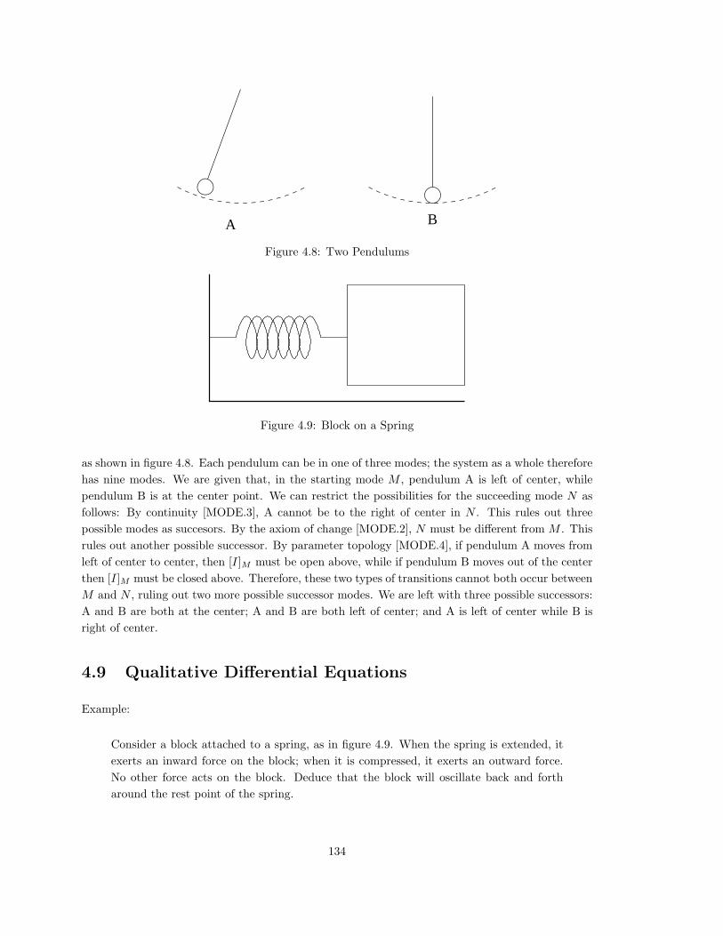
Figure 4.8: Two Pendulums

Figure 4.9: Block on a Spring

as shown in figure 4.8. Each pendulum can be in one of three modes; the system as a whole therefore

has nine modes. We are given that, in the starting mode M , pendulum A is left of center, while

pendulum B is at the center point. We can restrict the possibilities for the succeeding mode N as

follows: By continuity [MODE.3], A cannot be to the right of center in N . This rules out three

possible modes as succesors. By the axiom of change [MODE.2], N must be different from M . This

rules out another possible successor. By parameter topology [MODE.4], if pendulum A moves from

left of center to center, then [I]M must be open above, while if pendulum B moves out of the center

then [I]M must be closed above. Therefore, these two types of transitions cannot both occur between

M and N , ruling out two more possible successor modes. We are left with three possible successors:

A and B are both at the center; A and B are both left of center; and A is left of center while B is

right of center.

4.9 Qualitative Differential Equations

Example:

Consider a block attached to a spring, as in figure 4.9. When the spring is extended, it

exerts an inward force on the block; when it is compressed, it exerts an outward force.

No other force acts on the block. Deduce that the block will oscillate back and forth

around the rest point of the spring.

134

Parameters:

x — Position of the blockf — Force exerted on the block by the spring.

Atemporal constants:

m — Mass of the block.compress — Interval of compressed spring positions.rest — Rest length of the spring.expand — Interval of expanded spring positions.

Constraints:

f = m x. (Newton’s second law: The force is proportional to the acceleration.)[f] = rest − [x].

Table 4.13: Dynamics of the spring system

The problem here is to derive the behavior of a system of parameters over time, given constraints

obeyed by the parameters and their derivatives at each instant of time. These constraints derive in

part from the problem specifications and in part from a background knowledge of physics. Specifi-

cally, the problem can be formulated as shown in table 4.12. (We shall discuss how this formulation

can be derived from physical specifications in chapter 7.)

The givens thus form a system of differential relations; the problem is to solve them to derive a

characterization of parameters over time. However, the problem differs from the differential equations

in standard calculus courses in that the relation [f]=rest−[x] provide only a weak constraint between

the parameters, rather than an exact functional relation. The solution of the problem can therefore

at best come up with a partial characterization of the behavior, such as “the block oscillates,” rather

than a precise functional description. Specifically, the technique we will present will construct a mode

transition network, called an envisionment graph, for the solutions to the equations.

The basic technique for constructing an envisionment graph for such a system of equations

involves steps:

1. Translate any higher differential equations into a system of first order equations by introducing

the intermediate derivatives as new variables. In our example, we would convert the equation

“f = m·x” to the pair of equations “f = m · v; v = x”, by introducing the velocity v as a new

variable. All variable so introduced are derivatives, and so may be characterized in terms of

the signs { neg, 0, pos }.

2. Change all equations to relations on the signs or intervals of the parameters. In our example,

we would change the two equations introduced in (1) to the form “[f] = ∂v; [v] = ∂x.” (Recall

that ∂Q = sign(deriv(Q)). Note that we have used the fact that the mass m is positive). The

constraints “[f] = rest−[x]” is already in the proper form. The resultant equations are called

qualitative differential equations (QDE’s). Often, the problem is presented in the form of a set

of QDE’s, steps (1) and (2) having been performed implicitly in the problem formulation.

3. Let S be a parameter system containing all the parameters and derivatives from the equations

135

M0

M2

M4

M5

M7

M8

M3

M6

M1

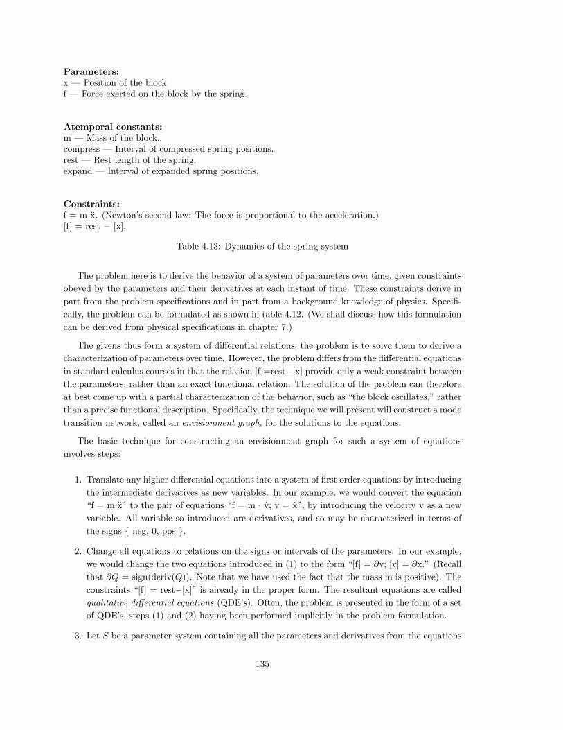
Figure 4.10: Envisionment Graph

QDE.1 (Mean value)If [Q]M < [Q]N and [Q]N is an open interval, then ∂QN=pos.If [Q]M > [Q]N and [Q]N is an open interval, then ∂QN=neg.If [Q]M < [Q]N and [Q]M is an open interval, then ∂QM=pos.If [Q]M > [Q]N and [Q]M is an open interval, then ∂QM=neg.

QDE.2 (Point transitions).If [Q]N is a point interval and ∂QN=posthen [Q]M < [Q]N < [Q]P and IN is a point interval.If [Q]N is a point interval and ∂QN=negthen [Q]M > [Q]N > [Q]P and IN is a point interval.

Table 4.14: Axioms for QDE’s

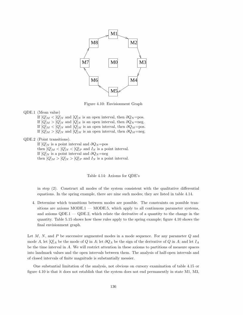
in step (2). Construct all modes of the system consistent with the qualitative differential

equations. In the spring example, there are nine such modes; they are listed in table 4.14.

4. Determine which transitions between modes are possible. The constraints on possible tran-

sitions are axioms MODE.1 — MODE.5, which apply to all continuous parameter systems,

and axioms QDE.1 — QDE.2, which relate the derivative of a quantity to the change in the

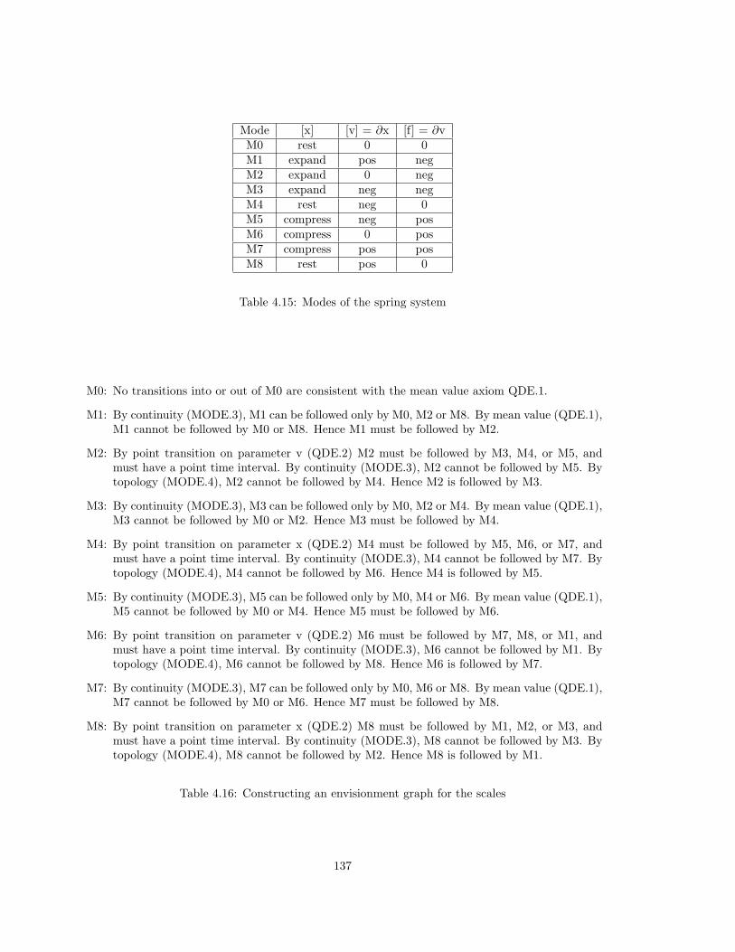
quantity. Table 5.15 shows how these rules apply to the spring example; figure 4.10 shows the

final envisionment graph.

Let M , N , and P be successive augmented modes in a mode sequence. For any parameter Q and

mode A, let [Q]A be the mode of Q in A; let ∂QA be the sign of the derivative of Q in A; and let IA

be the time interval in A. We will restrict attention in these axioms to partitions of measure spaces

into landmark values and the open intervals between them. The analysis of half-open intervals and

of closed intervals of finite magnitude is substantially messier.

One substantial limitation of the analysis, not obvious on cursory examination of table 4.15 or

figure 4.10 is that it does not establish that the system does not end permanently in state M1, M3,

136

Mode [x] [v] = ∂x [f] = ∂vM0 rest 0 0M1 expand pos negM2 expand 0 negM3 expand neg negM4 rest neg 0M5 compress neg posM6 compress 0 posM7 compress pos posM8 rest pos 0

Table 4.15: Modes of the spring system

M0: No transitions into or out of M0 are consistent with the mean value axiom QDE.1.

M1: By continuity (MODE.3), M1 can be followed only by M0, M2 or M8. By mean value (QDE.1),M1 cannot be followed by M0 or M8. Hence M1 must be followed by M2.

M2: By point transition on parameter v (QDE.2) M2 must be followed by M3, M4, or M5, andmust have a point time interval. By continuity (MODE.3), M2 cannot be followed by M5. Bytopology (MODE.4), M2 cannot be followed by M4. Hence M2 is followed by M3.

M3: By continuity (MODE.3), M3 can be followed only by M0, M2 or M4. By mean value (QDE.1),M3 cannot be followed by M0 or M2. Hence M3 must be followed by M4.

M4: By point transition on parameter x (QDE.2) M4 must be followed by M5, M6, or M7, andmust have a point time interval. By continuity (MODE.3), M4 cannot be followed by M7. Bytopology (MODE.4), M4 cannot be followed by M6. Hence M4 is followed by M5.

M5: By continuity (MODE.3), M5 can be followed only by M0, M4 or M6. By mean value (QDE.1),M5 cannot be followed by M0 or M4. Hence M5 must be followed by M6.

M6: By point transition on parameter v (QDE.2) M6 must be followed by M7, M8, or M1, andmust have a point time interval. By continuity (MODE.3), M6 cannot be followed by M1. Bytopology (MODE.4), M6 cannot be followed by M8. Hence M6 is followed by M7.

M7: By continuity (MODE.3), M7 can be followed only by M0, M6 or M8. By mean value (QDE.1),M7 cannot be followed by M0 or M6. Hence M7 must be followed by M8.

M8: By point transition on parameter x (QDE.2) M8 must be followed by M1, M2, or M3, andmust have a point time interval. By continuity (MODE.3), M8 cannot be followed by M3. Bytopology (MODE.4), M8 cannot be followed by M2. Hence M8 is followed by M1.

Table 4.16: Constructing an envisionment graph for the scales

137

A

C

D

B

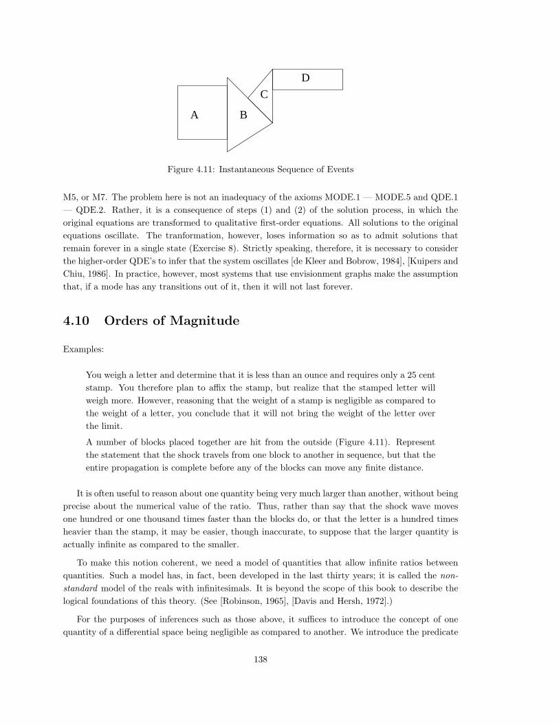
Figure 4.11: Instantaneous Sequence of Events

M5, or M7. The problem here is not an inadequacy of the axioms MODE.1 — MODE.5 and QDE.1

— QDE.2. Rather, it is a consequence of steps (1) and (2) of the solution process, in which the

original equations are transformed to qualitative first-order equations. All solutions to the original

equations oscillate. The tranformation, however, loses information so as to admit solutions that

remain forever in a single state (Exercise 8). Strictly speaking, therefore, it is necessary to consider

the higher-order QDE’s to infer that the system oscillates [de Kleer and Bobrow, 1984], [Kuipers and

Chiu, 1986]. In practice, however, most systems that use envisionment graphs make the assumption

that, if a mode has any transitions out of it, then it will not last forever.

4.10 Orders of Magnitude

Examples:

You weigh a letter and determine that it is less than an ounce and requires only a 25 cent

stamp. You therefore plan to affix the stamp, but realize that the stamped letter will

weigh more. However, reasoning that the weight of a stamp is negligible as compared to

the weight of a letter, you conclude that it will not bring the weight of the letter over

the limit.

A number of blocks placed together are hit from the outside (Figure 4.11). Represent

the statement that the shock travels from one block to another in sequence, but that the

entire propagation is complete before any of the blocks can move any finite distance.

It is often useful to reason about one quantity being very much larger than another, without being

precise about the numerical value of the ratio. Thus, rather than say that the shock wave moves

one hundred or one thousand times faster than the blocks do, or that the letter is a hundred times

heavier than the stamp, it may be easier, though inaccurate, to suppose that the larger quantity is

actually infinite as compared to the smaller.

To make this notion coherent, we need a model of quantities that allow infinite ratios between

quantities. Such a model has, in fact, been developed in the last thirty years; it is called the non-

standard model of the reals with infinitesimals. It is beyond the scope of this book to describe the

logical foundations of this theory. (See [Robinson, 1965], [Davis and Hersh, 1972].)

For the purposes of inferences such as those above, it suffices to introduce the concept of one

quantity of a differential space being negligible as compared to another. We introduce the predicate

138

X ≪ Y , which holds if X and Y are positive quantities and X is infinitesimal as compared to Y .

The predicate observes the following axioms:

NEG.1 X ≪ Y ⇒ 0 < X < Y .

NEG.2 [0 < W ≤ X ≪ Y ≤ Z] ⇒ W ≪ Z

NEG.3 [W ≪ Y ∧ X ≪ Y ] ⇒ (W + X) ≪ Y

NEG.4 [W ≪ X ∧ 0 < Y ] ⇒ W · Y ≪ X · Y

NEG.5 ∃X,Y X ≪ Y

NEG.6 Any first-order statement which is true of the standard real numbers and does not involve the

symbol ≪ is also true of the non-standard real numbers.

Axiom NEG.3 states that if both W and X are negligible compared to Y , then W +X is likewise

negligible. This directly contradicts the Archimedian property of the reals, that by adding any

positive quantity X to itself sufficiently often, one can exceed any given quantity Y . Also, the

completeness property of the reals, that every non-empty set with an upper bound has a least upper

bound, does not hold on the non-standard line; for any X > 0, the set of numbers Y such that

Y ≪ X does not have a least upper bound. (Neither of these properties can be fully axiomatized in

a first-order statement; hence their failure does not contract the axiom schema NEG.5)

We can now formalize our example of the letter and stamp. We introduce the predicate “close(X,Y )”

meaning that Y − X is of negligible magnitude as compared to Y .

close(X,Y ) ⇔ abs(Y − X) ≪ abs(Y )

We now specify that the letter is less than an ounce and not close to an ounce, and that the weight

of a stamp is negligible as compared to the weight of the letter. It then follows directly that the

letter plus stamp is less than an ounce.

Given: letter < ounce ∧ ¬close(letter,ounce).

stamp ≪ letter.

Infer: stamp + letter < ounce.

4.11 References

General: [Hayes, 1978] contains a general discussion of the nature and structure of measure spaces

used in commonsense reasoning, particularly physical reasoning. [Davis, 1987b] contains a survey

of the different kinds of arithmetic primitives needed for various commonsense domains with real-

valued measure spaces. [De Kleer and Weld, 1989] reprints many of the most significant papers

on reasoning about quantities for physical reasoning, including many of the papers cited below on

reasoning about collections of arithmetic relations, QDE’s, and orders of magnitude.

139

Intervals: The interval calculus has been studied almost exclusively as a representation for

temporal relations. In particular, [Van Benthem, 1983] contains a thorough study of the algebraic

and topological properties and logical power of various sets of axioms on the ordering of points and

intervals. The seminal AI paper on the interval calculus was [Allen, 1983], which introduced the

13 relations on intervals that we have used, and presented a transitivity table for combining them.

Further studies of the logical and computational properties of the interval calculus include [Vilain

and Kautz, 1986], [Allen and Hayes, 1985], [Ladkin, 1987].

Real-valued scales: The primary issue that has been in incorporating real arithmetic in AI

systems has been the organization and maintenance of an efficient system for ground atomic relations.

Propagation of exact values and of symbolic terms has been used to solve systems of equations in

[Sutherland, 1963], [Borning, 1977], [Sussman and Steele, 1980]. Waltz propagation on real intervals

has been applied to temporal reasoning in [Dean, 1984], and to spatial reasoning in [McDermott and

Davis, 1984] and [Davis, 1986]; [Davis, 1987b] has a formal analysis of the power of Waltz propagation

as applied to different classes of arithmetic relations. [Malik and Binford, 1983] advocates the use of

the simplex algorithm for the analysis of linear inequalities that arise in AI systems. The ACRONYM

system of [Brooks, 1981] has a powerful system for solving inequalities that may contain complex

algebraic and trigonometric terms for spatial reasoning. The BOUNDER program [Sacks, 1987]

uses a series of increasingly powerful and increasingly costly techniques for analyzing systems of

inequalities; it extends a similar system of Simmons’ [1986].

Sign calculus and QDE’s: In the AI literature, these two techniques were developed in tandem

for qualitative physical reasoning. QDE analysis was used implicitly in the NEWTON program [de

Kleer, 1975] (see section 6.2.6.) QDE’s and sign arithmetic were first developed as theories in their

own right in [de Kleer and Brown, 1985], [Kuipers, 1985], and [Williams, 1985]. [Kuipers, 1986]

is a careful and rigorous analyisis of the underlying theory. [Struss, 1989] studies the limits of

sign and QDE analysis. Since then a number of papers have extended the basic theory by using

richer information and more powerful analysis techniques. Many of these are collected in [de Kleer

and Weld, 1989]. Particularly significant are [de Kleer and Bobrow, 1984] and [Kuipers and Chiu,

1988] which study higher-order QDE equations; [Weld, 1986], which shows how QDE techniques

can be applied to certain discrete systems; and [Weld, 1988a] which analyses qualitatively how the

solutions to a differential equations are affected by perturbations to the parameters of the equations.

[Sacks, 1988] gives a more powerful qualitative analysis of exact differential equations, based on

approximating the equations with piecewise linear equations, and categorizing the solutions in terms

of transitions between regions of phase space.

Order of magnitude: The theory of non-standard real analysis was created by Abraham

Robinson [1965]; for a popular account, see [Davis and Hersh, 1972]. In the AI literature, non-

standard analysis has been applied to the automation of proofs in real analysis in [Ballantyne and

Bledsoe, 1977]; to the semantics of robotic programming languages in [Davis, 1984]; and to physical

reasoning in [Raiman, 1986]. [Davis, 1989b] and [Weld, 1988b] describe systems that combine order

of magnitude reasoning with QDE’s. [Mavrovouniotis and Stephanopoulos, 1989] gives a detailed

account of an inference engine for order-of-magnitude reasoning, and its application to process

engineering.

140

A B C

A

B

C

D

E

Sequence(A,Split(B,C),Split(D,E))

Sequence(A,B,C)

C

D

A

B

F

G

H

E

Sequence(Split(A,B),

Split(C, Sequence(D,E), F)

Split(G,H))

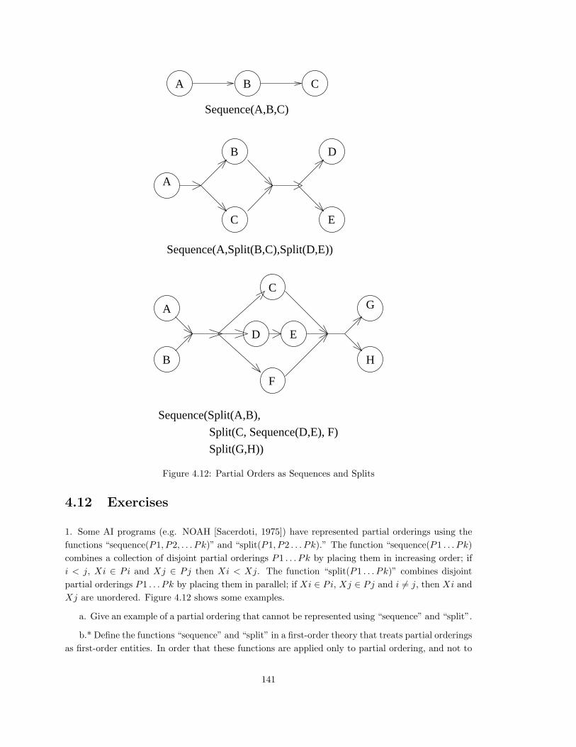
Figure 4.12: Partial Orders as Sequences and Splits

4.12 Exercises

1. Some AI programs (e.g. NOAH [Sacerdoti, 1975]) have represented partial orderings using the

functions “sequence(P1, P2, . . . Pk)” and “split(P1, P2 . . . Pk).” The function “sequence(P1 . . . Pk)

combines a collection of disjoint partial orderings P1 . . . Pk by placing them in increasing order; if

i < j, Xi ∈ Pi and Xj ∈ Pj then Xi < Xj. The function “split(P1 . . . Pk)” combines disjoint

partial orderings P1 . . . Pk by placing them in parallel; if Xi ∈ Pi, Xj ∈ Pj and i 6= j, then Xi and

Xj are unordered. Figure 4.12 shows some examples.

a. Give an example of a partial ordering that cannot be represented using “sequence” and “split”.

b.* Define the functions “sequence” and “split” in a first-order theory that treats partial orderings

as first-order entities. In order that these functions are applied only to partial ordering, and not to

141

simple elements, you may use a function “unary po(X)” which maps an element X to the partial

ordering containing only X. You may also assume for simplicity that “sequence” and “split” take

exactly two arguments. Thus the partial ordering with X1, X2, and X3 in that order could be

written

sequence(sequence(unary po(X1),unary po(X2)),unary po(X3))

Use the predicates “ordered(X1,X2, P )”, meaning that X1 precedes X2 in ordering P , and “element(X,P )”,

meaning that X is an element of ordering P .

c. Another representation of partial orderings [Meehan, 1975] is to associate a real interval with

each element of the partial ordering, and to define X as coming before Y in the ordering if the upper

bound of the interval of X less than the lower bound of Y . For example the labels X1 → [0, 1],

X2 → [2, 4], X3 → [3, 6], X4 → [5, 8] corresponds to the ordering X1 < X2 < X4, X1 < X3. Give

an example of a partial ordering that cannot be represented in this way.

d.* The representations in (a) and (c) are “compact,” in the sense that they require space linear in

the number of elements of the partial ordering. Show that there are more than 2cn2

different partial

orderings on n elements, for some constant c. Argue that therefore no compact representation of

partial orderings can represent all possible partial orderings.

2. Construct a transitivity table for the 13 interval relations discussed in section 4.2. This is a 13

by 13 table, in which each row is a relation between I and J , each column is a relation between J and

K, and the entry is the possible relations between I and K. For example, in the row “during(I, J)”

and the column “before(J,K)”, the entry is “{ before(I,K) }”. Note that some of the entries will

not be single valued, if there is more than one possible relation between I and K. For example, in

the row “starts(I, J)” and column “starts(K,J)”, the entry is “{starts(I,K), I = K, starts(K, I)}”.

3. Find an efficient (O(n2)) algorithm to solve the following problem: Given a collection of

atomic, ground interval constraints, determine whether the constraints are consistent. For example

the set {before(a,b), meets(a,c), overlap(c,b)} is consistent; it is satisfied by the interval a=[0,1],

b=[2,4], c=[1,3]. The set {before(a,b), meets(a,c), during(c,b)} is inconsistent.

4. Justify the statement in section 4.6, “Any equation on quantities can be converted into a

corresponding compatibility relation on the signs of the quantities. For example, from the equation

X + Y = P · Q, it is legitimate to infer the compatibility relation, [X] + [Y ] ∼ [P ] · [Q].”

5.* Justify the axiom MON.5 from table 4.8.

MON.5 [monotonic(QA,QB,QC, SG1) ∧ monotonic(QB,QC,QA, SG2) ∧ monotonic(QC,QA,QB, SG3)

] ⇒ SG1 · SG2 · SG3=neg

6. a. Find the mode transition network for the function f(t) = sin(t) sin(2t) using the signs of

the function and its derivative.

b. Find the mode transition network for the function f(t) = sin(t) sin(2t) using the signs of the

function and its first two derivatives.

7. If we modify the model of the block on the spring in section 4.9 by adding a damping force

proportional to the velocity, then the equations become,

142

f = m x.

v = x.

[f] = rest − [x] − [v].

Use the technique of section 4.9 to construct an envisionment graph for this problem.

8.a.* Consider the qualitative differential equation “[x] = −[x]” with the initial conditions

[x(0)]=pos, “[x[0]] = 0. Show that x(t)=0 for some positive t.

b.* Show that there are solutions to the pair of QDE’s “∂x=v; ∂v=−x” with the initial values

[x(0)]=pos, “[x[0]] = 0 such that x(t) is positive for all t>0.

143