Embed Size (px)
Citation preview
Quantum Cellular Automata:Theory and Applications
by
Carlos A. Perez Delgado
A thesis
presented to the University of Waterloo
in fulfilment of the
thesis requirement for the degree of
Doctor of Philosophy
in
Computer Science
Waterloo, Ontario, Canada, 2007
c©Carlos A. Perez Delgado 2007


I hereby declare that I am the sole author of this thesis. This is a true copy of the
thesis, including any required final revisions, as accepted by my examiners.
I understand that my thesis may be made electronically available to the public.
iii

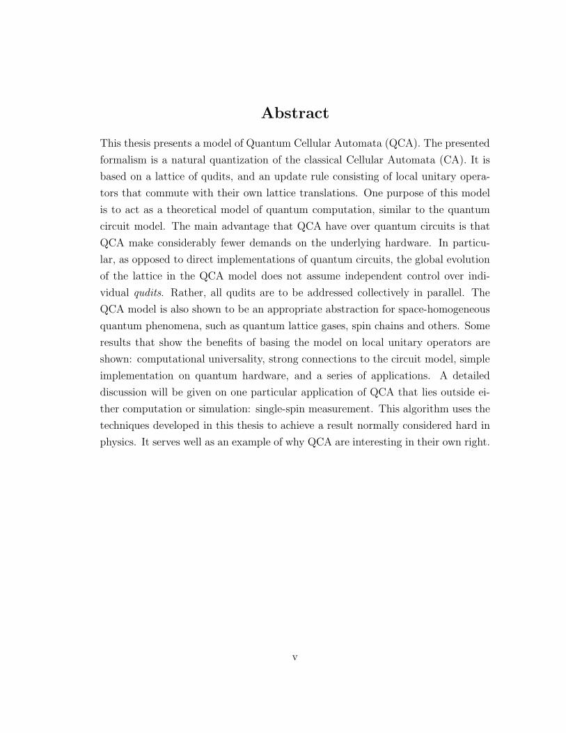
Abstract
This thesis presents a model of Quantum Cellular Automata (QCA). The presented
formalism is a natural quantization of the classical Cellular Automata (CA). It is
based on a lattice of qudits, and an update rule consisting of local unitary opera-
tors that commute with their own lattice translations. One purpose of this model
is to act as a theoretical model of quantum computation, similar to the quantum
circuit model. The main advantage that QCA have over quantum circuits is that
QCA make considerably fewer demands on the underlying hardware. In particu-
lar, as opposed to direct implementations of quantum circuits, the global evolution
of the lattice in the QCA model does not assume independent control over indi-
vidual qudits. Rather, all qudits are to be addressed collectively in parallel. The
QCA model is also shown to be an appropriate abstraction for space-homogeneous
quantum phenomena, such as quantum lattice gases, spin chains and others. Some
results that show the benefits of basing the model on local unitary operators are
shown: computational universality, strong connections to the circuit model, simple
implementation on quantum hardware, and a series of applications. A detailed
discussion will be given on one particular application of QCA that lies outside ei-
ther computation or simulation: single-spin measurement. This algorithm uses the
techniques developed in this thesis to achieve a result normally considered hard in
physics. It serves well as an example of why QCA are interesting in their own right.
v

Acknowledgements
I would like to extend my deepest thanks to my supervisor, Prof. Michele Mosca.
He has consistently pushed me to become a better scientist. Also, I would like to
thank Prof. David G. Cory. His input had a profound impact on the research I
carried during my PhD studies. I would also like to thank the members of my PhD
thesis committee: Prof. Raymond Laflamme, Prof. John Watrous, Prof. Gregor
Weihs, and Prof. Simon Benjamin. Their criticism and remarks have helped to
shape not just this thesis, but my own research.
I would like to thank my co-authors. I would also like to extend my thanks to
Dr. Jonathan Baugh, Niel de Beaudrap, Anne Broadbent, Dr. Fay Dowker, Dr.
David Evans, Phillip Kaye, Martin Laforest, Annika Niehage, Dr. Pranab Sen, and
Robert H. Warren for useful and stimulating conversations.
I’d like to thank the people that make up the Institute for Quantum Computing
at the University of Waterloo—with special thanks to Wendy Reibel—and the
School of Computer Science.
Finally, I would like to thank three very special and important people in my
life. The first two, Roberto Perez Delgado—my brother—and Marıa de Guadalupe
Delgado de Perez—my mother—have been with me since I can remember, and
have consistently provided me strength and support. Last, but by no means least,
Joanna Ziembicka deserves special mention. She has become a central part in my
life, helping to provide meaning to everything I do.
vii

Dedication
This thesis is lovingly dedicated to the memory of J. Antonio Perez-Gonzalez 1953–
2003. Though a physicist by trade, he was a father by calling. He continues to be
the inspiration, not just for my work, but for who I am.
ix

Contents
1 Introduction 1
1.1 Summary of Results . . . . . . . . . . . . . . . . . . . . . . . . . . 2
1.2 What QCA Are Not . . . . . . . . . . . . . . . . . . . . . . . . . . 4
1.3 Organization and Layout . . . . . . . . . . . . . . . . . . . . . . . . 6
1.4 A Note on Notation . . . . . . . . . . . . . . . . . . . . . . . . . . . 8
I Theory 11
2 Cellular Automata 13
2.1 Reversible, Block, and Partitioned CA . . . . . . . . . . . . . . . . 14
2.2 Totalistic CA . . . . . . . . . . . . . . . . . . . . . . . . . . . . . . 18
3 Quantum Cellular Automata 21
3.1 Local Unitary QCA . . . . . . . . . . . . . . . . . . . . . . . . . . 22
3.1.1 Model Requirements . . . . . . . . . . . . . . . . . . . . . . 22
3.1.2 A First Approach . . . . . . . . . . . . . . . . . . . . . . . . 22
3.1.3 A New Approach . . . . . . . . . . . . . . . . . . . . . . . . 27
3.1.4 Quiescent States . . . . . . . . . . . . . . . . . . . . . . . . 29
4 Quantum Circuits and Universality 33
4.1 Simulation of QCA by Quantum Circuits . . . . . . . . . . . . . . 34
4.2 Simulation of Quantum Circuits by QCA . . . . . . . . . . . . . . 36
xi
5 Previous QCA Models 39
5.1 Watrous-van Dam QCA . . . . . . . . . . . . . . . . . . . . . . . . 39
5.2 Schumacher-Werner QCA . . . . . . . . . . . . . . . . . . . . . . . 42
5.3 Other Models . . . . . . . . . . . . . . . . . . . . . . . . . . . . . . 46
6 Universality of 1d LUQCA 47
6.1 Quantum Turing Machines . . . . . . . . . . . . . . . . . . . . . . . 48
6.2 Proof of Universality . . . . . . . . . . . . . . . . . . . . . . . . . . 51
II Applications 55
7 Modelling Physical Systems 57
7.1 Spin Chains . . . . . . . . . . . . . . . . . . . . . . . . . . . . . . . 57
7.2 Quantum Lattice Gases . . . . . . . . . . . . . . . . . . . . . . . . 60
8 Quantum Computation 65
8.1 Coloured QCA . . . . . . . . . . . . . . . . . . . . . . . . . . . . . 66
9 Single Spin Measurement 71
9.1 Problem Description . . . . . . . . . . . . . . . . . . . . . . . . . . 72
9.2 Algorithm Development . . . . . . . . . . . . . . . . . . . . . . . . 74
9.3 Algorithm Analysis . . . . . . . . . . . . . . . . . . . . . . . . . . 79
9.3.1 Methodology . . . . . . . . . . . . . . . . . . . . . . . . . . 89
9.4 Physical Implementation . . . . . . . . . . . . . . . . . . . . . . . 91
10 Further Directions and Conclusions 99
10.1 Dissipative QCA . . . . . . . . . . . . . . . . . . . . . . . . . . . . 99
10.1.1 Algorithmic Cooling with QCA . . . . . . . . . . . . . . . . 102
10.1.2 Fault-Tolerant QCA . . . . . . . . . . . . . . . . . . . . . . 104
10.2 Further Physical Implementations of QCA . . . . . . . . . . . . . . 105
10.3 Modifications and Further Applications of Spin-Amplification . . . . 105
10.3.1 Using Different Lattice Structures . . . . . . . . . . . . . . . 106
xii
10.3.2 Cat State Creation and Verification . . . . . . . . . . . . . . 106
10.4 Further Simulations of Physical Systems . . . . . . . . . . . . . . . 113
10.4.1 The Universe as a QCA . . . . . . . . . . . . . . . . . . . . 114
10.5 Closing Remarks . . . . . . . . . . . . . . . . . . . . . . . . . . . . 115
Bibliography 117
xiii

List of Figures
1.1 Thesis Organization Chart . . . . . . . . . . . . . . . . . . . . . . 7
2.1 A Simple Cellular Automata Rule . . . . . . . . . . . . . . . . . . . 14
2.2 A Simple Cellular Automaton’s Evolution in Time . . . . . . . . . . 15
2.3 Margolus Cellular Automaton . . . . . . . . . . . . . . . . . . . . . 17
2.4 Partitioned CA . . . . . . . . . . . . . . . . . . . . . . . . . . . . . 18
3.1 Shift-right No-go Lemma . . . . . . . . . . . . . . . . . . . . . . . . 25
3.2 Past lightcone of a region S . . . . . . . . . . . . . . . . . . . . . . 31
4.1 Quantum Circuit simulation of a QCA Update step . . . . . . . . . 35
4.2 Universal QCA Update Rule . . . . . . . . . . . . . . . . . . . . . . 38
5.1 Watrous QCA . . . . . . . . . . . . . . . . . . . . . . . . . . . . . . 41
5.2 Watrous QCA expressed as a Local Unitary QCA . . . . . . . . . . 42
6.1 A Turing Machine . . . . . . . . . . . . . . . . . . . . . . . . . . . . 48
7.1 Feynman path sum of a particle. . . . . . . . . . . . . . . . . . . . . 61
7.2 Quantum walk on a lattice. . . . . . . . . . . . . . . . . . . . . . . 63
9.1 A simple quantum circuit that implements spin amplification. . . . 73
9.2 Cube lattice . . . . . . . . . . . . . . . . . . . . . . . . . . . . . . . 74
9.3 Pyramid lattice . . . . . . . . . . . . . . . . . . . . . . . . . . . . . 76
9.4 Coloured cube lattice . . . . . . . . . . . . . . . . . . . . . . . . . . 77
9.5 Coloured pyramid lattice . . . . . . . . . . . . . . . . . . . . . . . . 78
xv
9.6 Signal Power as a function of error rate ( ǫ2 = 10−4). . . . . . . . . 84
9.7 Signal Power as a function of error rate (ǫ2 = ǫ1). . . . . . . . . . . 85
9.8 Signal Power as a function of error rate (ǫ2 = ǫ21). . . . . . . . . . . 86
9.9 Signal Power as a function of error rate (ǫ2 = 10−4, edge cooling). . 87
9.10 Signal Power as a function of error rate ( ǫ2 = ǫ21, edge cooling). . . 88
9.11 Signal Power as a function of ancilla size. . . . . . . . . . . . . . . . 89
9.12 Signal Power Histogram . . . . . . . . . . . . . . . . . . . . . . . . 90
9.13 Ideal NMR Spectrum . . . . . . . . . . . . . . . . . . . . . . . . . . 92
9.14 Actual NMR Spectrum . . . . . . . . . . . . . . . . . . . . . . . . . 94
9.15 Spectrum with homonuclear coupling suppressed . . . . . . . . . . . 95
9.16 Pulse Sequence . . . . . . . . . . . . . . . . . . . . . . . . . . . . . 96
10.1 Circuit for three bit majority . . . . . . . . . . . . . . . . . . . . . 103
xvi
Chapter 1
Introduction
This thesis presents the theory and applications of Quantum Cellular Automata
(QCA). One of the main contributions presented here is the introduction of a new
model of QCA, the local unitary QCA or LUQCA for short.
The Cellular Automaton (CA) is a computational model that has been studied
for many decades [vN51,vN66]. It is a fairly simple, yet powerful model of compu-
tation that has been shown to be Turing complete [vN66]. It is based on massive
parallelism and simple, locally constrained instructions, making it ideal for various
applications. Although usually simulated in software, CA hardware implementa-
tions have also been developed [OMH87,OTM88]. This is due to the fact that CA
are very effective at simulating many classical physical systems, including gas dis-
persion, fluids dynamics, ice formation, and even biological colony growth [CD98].
All of these characteristics make CA a very strong tool for going from a physical
system in nature, to a mathematical model, to an implemented physical simulation.
More recently, the idea of Quantum Cellular Automata (QCA) has emerged.
Several theoretical mathematical models have been proposed [SW04,vD96,Wat95,
PDC05]. However, there is a lack of applications developed within these models.
On the other hand, ad hoc models for specific applications like quantum lattice
gases [Mey96a,BT98], among others [FKK07], have been developed. Several pro-
posals for scalable quantum computation (QC) have been developed that use ideas
and tools related to QCA [FXBJ07,FT06,VC06,Ben00,BB03,Llo93].
1
2 CHAPTER 1. INTRODUCTION
Also, several QCA constructs have been shown to be capable of universal quan-
tum computation [Rau05, SFW06]. Finally, QCA tools have been used to solve,
or propose solutions to, particular problems in physics [ICJ+06, KBST05, LK05,
PDMCC06,WJ06,LB06].
However, there does not exist a comprehensive model of QCA that encompasses
these different views and techniques. Rather, each set of authors defines QCA
in their own particular fashion. In short, there is a lack of a generally accepted
QCA model that has all the attributes of the CA model mentioned above: sim-
ple to describe; computationally powerful and expressive; efficiently implementable
in quantum software and hardware; and able to efficiently and effectively model
appropriate physical phenomena.
The purpose of this thesis is to provide such a model.
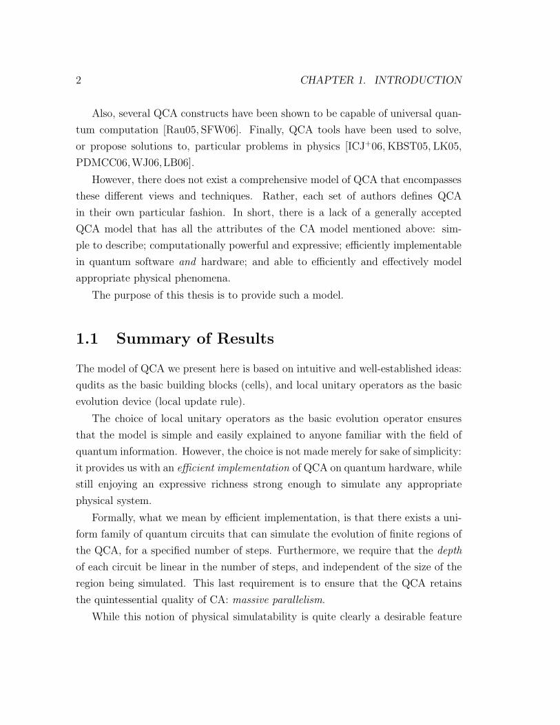
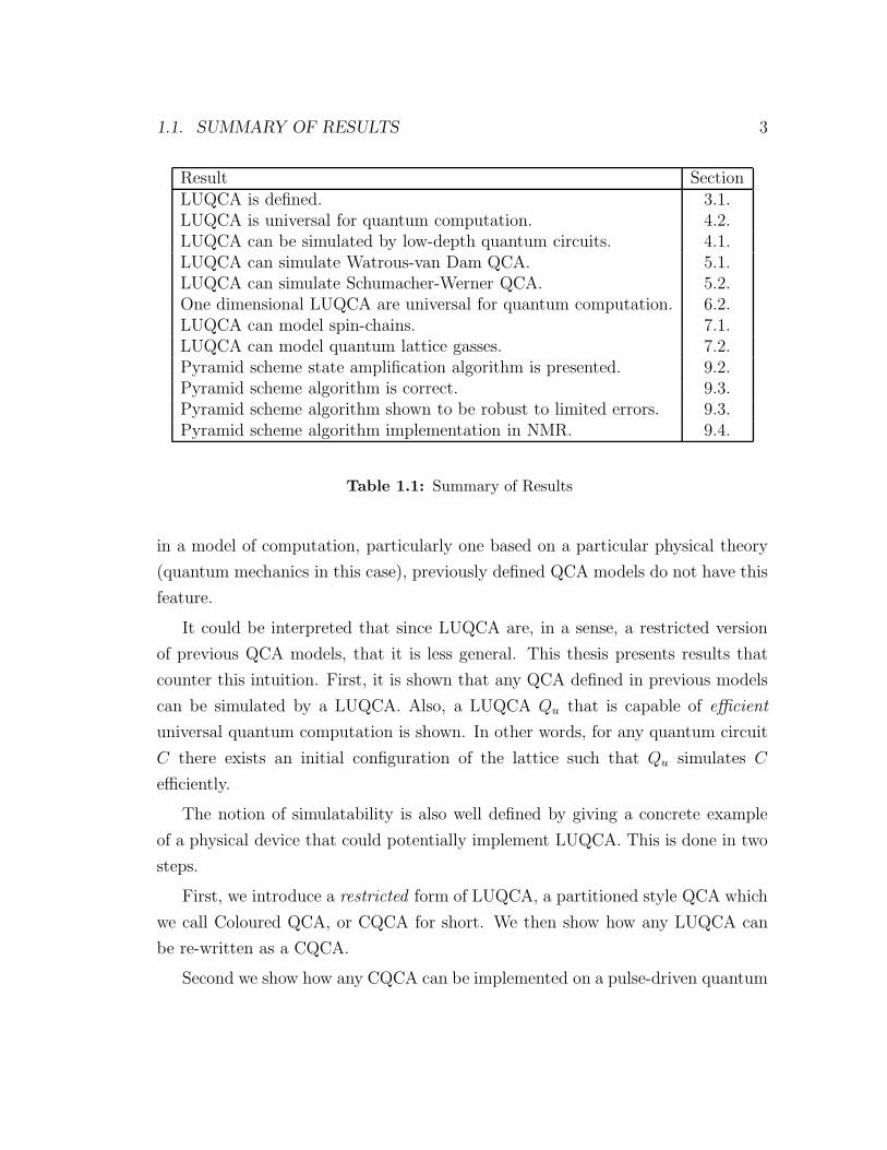
1.1 Summary of Results
The model of QCA we present here is based on intuitive and well-established ideas:
qudits as the basic building blocks (cells), and local unitary operators as the basic
evolution device (local update rule).
The choice of local unitary operators as the basic evolution operator ensures
that the model is simple and easily explained to anyone familiar with the field of
quantum information. However, the choice is not made merely for sake of simplicity:
it provides us with an efficient implementation of QCA on quantum hardware, while
still enjoying an expressive richness strong enough to simulate any appropriate
physical system.
Formally, what we mean by efficient implementation, is that there exists a uni-
form family of quantum circuits that can simulate the evolution of finite regions of
the QCA, for a specified number of steps. Furthermore, we require that the depth
of each circuit be linear in the number of steps, and independent of the size of the
region being simulated. This last requirement is to ensure that the QCA retains
the quintessential quality of CA: massive parallelism.
While this notion of physical simulatability is quite clearly a desirable feature
1.1. SUMMARY OF RESULTS 3
Result SectionLUQCA is defined. 3.1.LUQCA is universal for quantum computation. 4.2.LUQCA can be simulated by low-depth quantum circuits. 4.1.LUQCA can simulate Watrous-van Dam QCA. 5.1.LUQCA can simulate Schumacher-Werner QCA. 5.2.One dimensional LUQCA are universal for quantum computation. 6.2.LUQCA can model spin-chains. 7.1.LUQCA can model quantum lattice gasses. 7.2.Pyramid scheme state amplification algorithm is presented. 9.2.Pyramid scheme algorithm is correct. 9.3.Pyramid scheme algorithm shown to be robust to limited errors. 9.3.Pyramid scheme algorithm implementation in NMR. 9.4.
Table 1.1: Summary of Results
in a model of computation, particularly one based on a particular physical theory
(quantum mechanics in this case), previously defined QCA models do not have this
feature.
It could be interpreted that since LUQCA are, in a sense, a restricted version
of previous QCA models, that it is less general. This thesis presents results that
counter this intuition. First, it is shown that any QCA defined in previous models
can be simulated by a LUQCA. Also, a LUQCA Qu that is capable of efficient
universal quantum computation is shown. In other words, for any quantum circuit
C there exists an initial configuration of the lattice such that Qu simulates C
efficiently.
The notion of simulatability is also well defined by giving a concrete example
of a physical device that could potentially implement LUQCA. This is done in two
steps.
First, we introduce a restricted form of LUQCA, a partitioned style QCA which
we call Coloured QCA, or CQCA for short. We then show how any LUQCA can
be re-written as a CQCA.
Second we show how any CQCA can be implemented on a pulse-driven quantum
4 CHAPTER 1. INTRODUCTION
computer, as introduced by Lloyd [Llo93], and further refined by Benjamin [Ben00,
BB04] among others.
Another important series of results presented in this thesis pertain to the ap-
plication value of QCA in general, and LUQCA in particular. In particular, there
is an emphasis on modelling quantum physical systems with repetitive structure
using LUQCA.
These results, together with those mentioned above about the implementability
of LUQCA, provide a constructive method for actually simulating physical systems
of particular type.
Finally, we present one application of QCA in great detail. We present a problem
of great interest to be solved, namely the measurement of a single spin in the context
of NMR QIP. Then, we set out to solve this problem using the theory of QCA.
This application of QCA is interesting and important in its own right, as it
describes a procedure for achieving a goal that is considered hard in experimental
physics. The solution given also provides a prime example of the expressive powers
of QCA. The problem is abstracted in the QCA model, allowing us to work with it
without referring to any actual underlying physical systems, until necessary.
We start with a description of the problem, give an abstraction based on QCA,
provide an algorithm to solve this problem within the abstraction, and then use
the tools we have developed to transform the theoretical model into a proposed
physical implementation.
This showcases the ultimate raison d’etre of QCA: providing an easy to use,
yet powerful, abstraction for working with molecular scale spatially homogeneous
systems.
Table 1.1 presents a summary of the results presented in this thesis.
1.2 What QCA Are Not
It is important to remark that QCA are not Globally Controlled Quantum Arrays
(GCQA).
In this thesis we will be discussing GCQA, or pulse-driven quantum comput-
1.2. WHAT QCA ARE NOT 5
ers [Llo93, Ben00], inter alia, as a possible implementation of QCA on quantum
hardware. However, this should not be taken to mean that the two paradigms are
equivalent.
A GCQA is centred around the idea of doing computation on large arrays of
simple quantum systems, without locally addressing them. GCQA divide their
lattice of cells, or qudits, into subsets each of which can be addressed collectively.
The canonical example, due to Lloyd [Llo93], is a chain of three species of qudits
A, B, and C, arranged in a repeating fashion,
. . .− A− B − C −A− B − C − A− B − C −A− B − C − A− B − C − . . .
The first major distinction with QCA comes from the fact that sequence of
pulses applied to these subsets of qudits are arbitrary, and do not necessarily follow
a time-homogenous pattern.
The second, is that although Lloyd’s construction is space homogenous, GCQA
are not constrained in such a fashion. More recently, GCQA have been proposed
that have less spatially homogenous structures [FT07]. For instance,
. . .−A−B −A−B − A− A− B − B − B − B −B −B − . . .
As a model of computation one can say that QCA are more restricted than
GCQA. At the same time, QCA are more than just a model of computation. They
serve also as models of physical phenomena. It can be argued that QCA are, in a
sense, a more fundamental construct.
There is one last concept that needs to be addressed here. In a series of papers,
Lent et. al.—see, e.g. [LTPB93]—develop a method for doing classical computation
by using the ground state of a system consisting of a series of quantum dots. They
call this proposal a ‘quantum cellular automata’.
While it is true that the dots interact with each other through magnetic cou-
plings, the manner of the computation in no way resembles what is the accepted
definition of a cellular automata. Rather, energy is delivered to the quantum dot
lattice through its boundaries, so that the ground state of the system yields the
6 CHAPTER 1. INTRODUCTION
computational result. While this paradigm is no doubt innovative, using the term
‘quantum cellular automata’ to describe it is misleading, and even incorrect. The
term ‘ground state computing’ is perhaps more appropriate.
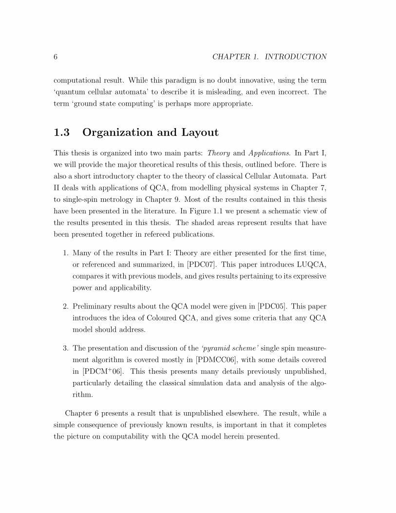
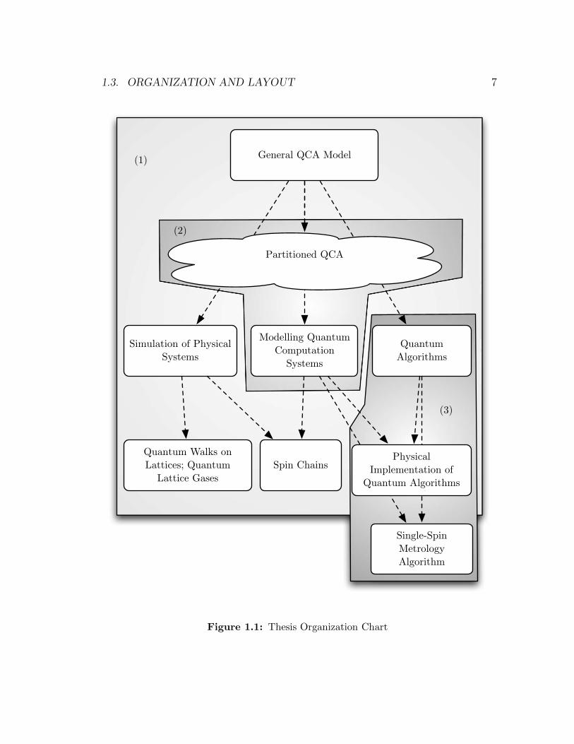
1.3 Organization and Layout
This thesis is organized into two main parts: Theory and Applications. In Part I,
we will provide the major theoretical results of this thesis, outlined before. There is
also a short introductory chapter to the theory of classical Cellular Automata. Part
II deals with applications of QCA, from modelling physical systems in Chapter 7,
to single-spin metrology in Chapter 9. Most of the results contained in this thesis
have been presented in the literature. In Figure 1.1 we present a schematic view of
the results presented in this thesis. The shaded areas represent results that have
been presented together in refereed publications.
1. Many of the results in Part I: Theory are either presented for the first time,
or referenced and summarized, in [PDC07]. This paper introduces LUQCA,
compares it with previous models, and gives results pertaining to its expressive
power and applicability.
2. Preliminary results about the QCA model were given in [PDC05]. This paper
introduces the idea of Coloured QCA, and gives some criteria that any QCA
model should address.
3. The presentation and discussion of the ‘pyramid scheme’ single spin measure-
ment algorithm is covered mostly in [PDMCC06], with some details covered
in [PDCM+06]. This thesis presents many details previously unpublished,
particularly detailing the classical simulation data and analysis of the algo-
rithm.
Chapter 6 presents a result that is unpublished elsewhere. The result, while a
simple consequence of previously known results, is important in that it completes
the picture on computability with the QCA model herein presented.
1.3. ORGANIZATION AND LAYOUT 7
General QCA Model
Single-Spin
Metrology
Algorithm
Quantum Walks on
Lattices; Quantum
Lattice Gases
Spin Chains
Simulation of Physical
Systems
Quantum
Algorithms
Modelling Quantum
Computation
Systems
Partitioned QCA
Physical
Implementation of
Quantum Algorithms
(1)
(2)
(3)
Figure 1.1: Thesis Organization Chart
8 CHAPTER 1. INTRODUCTION
Chapter 10 collects and presents all the avenues of research that have been
opened by the results from the previous chapters. Any results presented there
should be taken to represent work in progress at the time of this writing.
All of the work presented in this thesis has been done under the supervision of
Prof. Michele Mosca. Chapter 9 presents work done in collaboration with Prof.
David G. Cory, and Paola Cappellaro at MIT. Chapter 7 presents work developed
during an author’s visit to MIT, and was inspired in part by conversation with
Zhiying Chen. Some of the ideas in Chapter 10 about QCA models of nature are
inspired by conversations with Prof. Fay Dowker. The work presented in Part I of
this thesis is joint work with Donny Cheung.
1.4 A Note on Notation
In this thesis we will be adopting the following notation.
The letters j, k, ℓ,m will be reserved for indices. The letter i will be used
exclusively to denote the square root of −1. Functions will be denoted by lowercase
Latin letters f, g, h.
Alphabets will be denoted by the uppercase Greek letters Σ,Γ, etc. Symbols in
an alphabet will be denoted with the appropriate lowercase Greek letter, indexed
as necessary. For instance, σ1, σ2, . . . , σk ∈ Σ.
Sometimes we will refer to a classical physical system that can be in any one of
N states, each labelled by an element of Σ. In such cases we will not distinguish
between the state and the label. For instance, we can say that the system is in
state σj ∈ Σ.
When referring to a quantum system, with states labelled by Σ we will denote
the actual states by |σ〉, to make a distinction from classical systems. The state
space of such a quantum system is the complex Euclidean space, sometimes referred
to as a finite Hilbert space, spanned by the states |σ〉σ∈Σ. We shall call this space
the Hilbert space of the system,
HΣ = span (|σ〉σ∈Σ) .
1.4. A NOTE ON NOTATION 9
Arbitrary states in such a Hilbert space will be denoted |ψ〉 , |φ〉 etc.
In the latter part of this thesis we will be discussing Hamiltonians of different
systems. We will also use H to denote Hamiltonians. This will not be a cause of
confusion as we will never use H to denote both Hamiltonians and Hilbert spaces
at the same time.
We will denote the set of all unitary operators acting on a space HΣ as U (HΣ).
Unitary operators will be denoted by uppercase slanted Latin letters U, V , sub-
indexed as necessary.
The set of density operators over a Hilbert space HΣ will be denoted as D (HΣ).
Individual density operators will be denoted as ρ, ρ0, ρ1 etc.
The set of completely positive trace preserving (CPTP) maps over a Hilbert
space will be denoted as A (HΣ). We will denote particular CPTP maps with
uppercase Greek letters Φ, Ξ, sub-indexed as needed.
This thesis is intended for a wide audience: computer scientists, mathemati-
cians, physicists, quantum chemists, etc. As such the decision to use the Dirac
notation may be slightly controversial. While it is almost universally used within
the quantum mechanics, and quantum information, communities it almost as uni-
versally ignored outside of it. The choice to use the Dirac notation is based on its
elegance, ease of use, and expressive abilities.
A ket |ψ〉 can be simply regarded as a column vector, with the corresponding
bra, 〈ψ| its conjugate transpose. Everything else easily follows: 〈φ| |ψ〉 abbreviated
〈φ|ψ〉 is simply the inner product of |ψ〉 and |φ〉. The outer product of the two
is simply |ψ〉 〈φ|. The tensor product of two states |ψ〉 ⊗ |φ〉, can sometimes be
abbreviated as |ψ, φ〉.


Part I
Theory
11

Chapter 2
Cellular Automata
In this chapter we give a brief introduction to the classical theory of cellular au-
tomata. We will first present the model intuitively, and then give a more formal
definition. We will need the definitions and results presented in this chapter later
on in this thesis.
In the most simple terms, a cellular automaton is a lattice of cells, each of which
is in one of a finite set of states, at any one moment in time. At each discrete time
step the state of each and every cell cell is updated according to some local transition
function. The input of this function is the current state of the corresponding cell,
and the states of the cells in a finite sized neighbourhood around this cell.
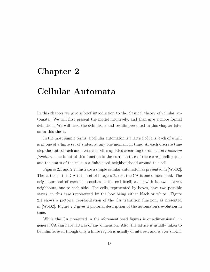
Figures 2.1 and 2.2 illustrate a simple cellular automaton as presented in [Wol02].
The lattice of this CA is the set of integers Z, i.e., the CA is one-dimensional. The
neighbourhood of each cell consists of the cell itself, along with its two nearest
neighbours, one to each side. The cells, represented by boxes, have two possible
states, in this case represented by the box being either black or white. Figure
2.1 shows a pictorial representation of the CA transition function, as presented
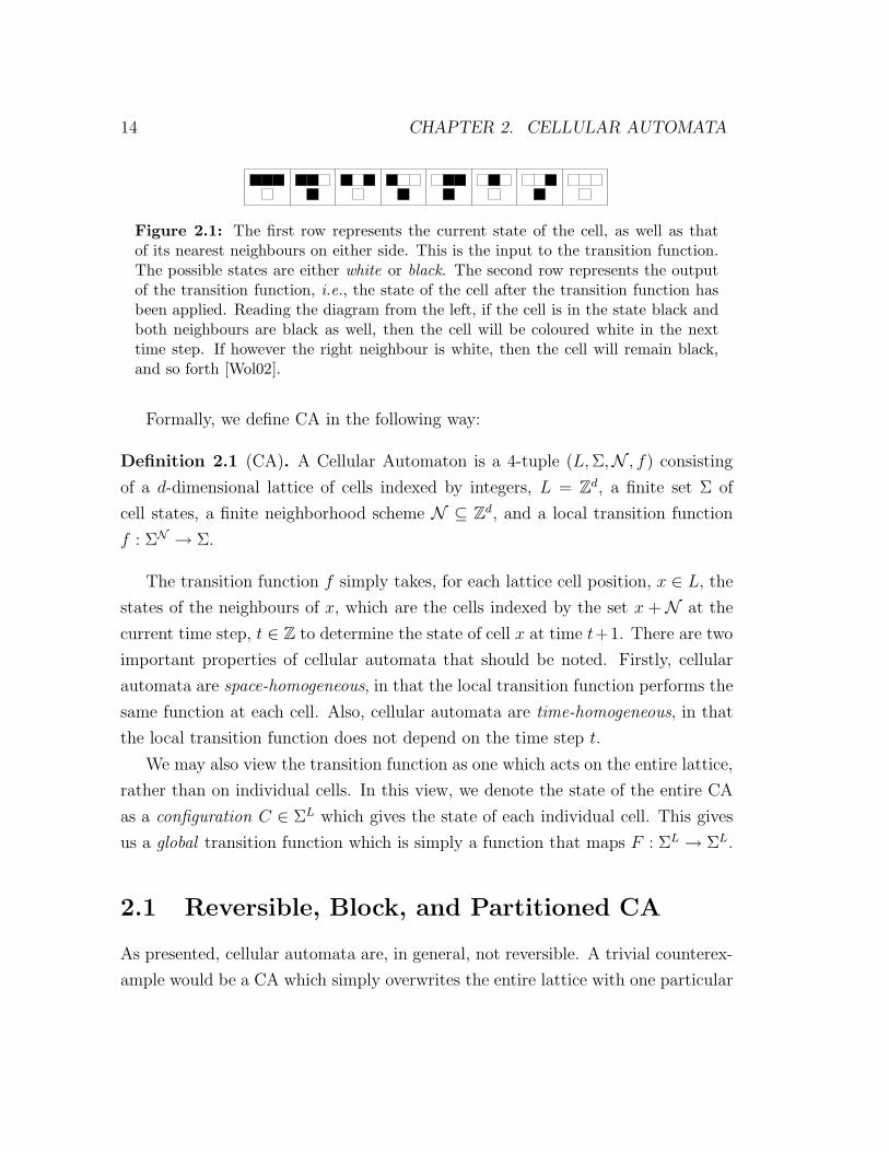
in [Wol02]. Figure 2.2 gives a pictorial description of the automaton’s evolution in
time.
While the CA presented in the aforementioned figures is one-dimensional, in
general CA can have lattices of any dimension. Also, the lattice is usually taken to
be infinite, even though only a finite region is usually of interest, and is ever shown.
13
14 CHAPTER 2. CELLULAR AUTOMATA
Figure 2.1: The first row represents the current state of the cell, as well as thatof its nearest neighbours on either side. This is the input to the transition function.The possible states are either white or black. The second row represents the outputof the transition function, i.e., the state of the cell after the transition function hasbeen applied. Reading the diagram from the left, if the cell is in the state black andboth neighbours are black as well, then the cell will be coloured white in the nexttime step. If however the right neighbour is white, then the cell will remain black,and so forth [Wol02].
Formally, we define CA in the following way:
Definition 2.1 (CA). A Cellular Automaton is a 4-tuple (L,Σ,N , f) consisting
of a d-dimensional lattice of cells indexed by integers, L = Zd, a finite set Σ of
cell states, a finite neighborhood scheme N ⊆ Zd, and a local transition function
f : ΣN → Σ.
The transition function f simply takes, for each lattice cell position, x ∈ L, the
states of the neighbours of x, which are the cells indexed by the set x + N at the
current time step, t ∈ Z to determine the state of cell x at time t+1. There are two
important properties of cellular automata that should be noted. Firstly, cellular
automata are space-homogeneous, in that the local transition function performs the
same function at each cell. Also, cellular automata are time-homogeneous, in that
the local transition function does not depend on the time step t.
We may also view the transition function as one which acts on the entire lattice,
rather than on individual cells. In this view, we denote the state of the entire CA
as a configuration C ∈ ΣL which gives the state of each individual cell. This gives
us a global transition function which is simply a function that maps F : ΣL → ΣL.
2.1 Reversible, Block, and Partitioned CA
As presented, cellular automata are, in general, not reversible. A trivial counterex-
ample would be a CA which simply overwrites the entire lattice with one particular
2.1. REVERSIBLE, BLOCK, AND PARTITIONED CA 15
Figure 2.2: From top to bottom, left to right, the figures represent the evolutionin time of the CA described in Figure 2.1. The initial configuration, shown in thetop left image, is a single cell coloured black, while all others are white. Time flowsdownwards. Each subsequent image depicts the current state of the automaton, andall stages since the initial one [Wol02].
symbol.
A CA is reversible if for any configuration C ∈ ΣL, and time step t ∈ Z there
exists a unique predecessor configuration C ′ such that C = F (C ′, t). It is known
that any Turing machine can be simulated using a reversible CA [Tof77], so no
computational power is lost by this restriction.
One method that is used to construct reversible cellular automata is that of
blocks and partitioning. In a block CA, the transition function is composed of local
operations on individual units blocks of the lattice. If each of these local operations
is reversible, then the evolution of the CA as a whole is also guaranteed to be
reversible.
In order to formally define the block CA, we must expand the definition of cellu-
lar automata, as block CA are neither time-homogeneous nor space-homogeneous in
general. They are, however, periodic in both space and time, and thus we set both
a time period, T ∈ Z, with T ≥ 1 and a space period, given as a d-dimensional sub-
lattice, S of L = Zd. The sublattice S can be defined using a set vk : k = 1, . . . , d
16 CHAPTER 2. CELLULAR AUTOMATA
of d linearly independent vectors from L = Zd as:
S =
d∑
k=1
akvk : ak ∈ Z
.
Definition 2.2. For a given fixed sublattice S ⊆ Zd, we define a block, B ⊆ Zd
as a finite subset of Zd such that (B + s1) ∩ (B + s2) = ∅ for any s1, s2 ∈ S with
s1 6= s2, and such that ⋃
s∈S
(B + s) = Zd.
The main idea of the block CA is that at different time steps, we act on a
different block partitioning of the lattice. We are now ready to formally define the
block CA.
Definition 2.3. A Block CA is a 6-tuple (L, S, T,Σ,B,F) consisting of
1. a d-dimensional lattice of cells indexed by integers, L = Zd;
2. a d-dimensional sublattice S ⊆ L;
3. a time period T ≥ 1;
4. a finite set Σ of cell states;
5. a block scheme B, which is a sequence B0, B1, . . . , BT−1 consisting of T
blocks relative to the sublattice S; and
6. a local transition function scheme F , which is a set f0, f1, . . . , fT−1 of re-
versible local transition functions which map ft : ΣBt → ΣBt .
At time step t + kT for 0 ≤ t < T and k ∈ Z, we perform ft on every block
Bt + s, where s ∈ S.
If every fi ∈ F is reversible, then the CA is reversible. In order to find the reverse
of the CA, we simply give the reverse block scheme, B = BT−1, . . . , B1, B0, and
the reverse function scheme, F = f−1T−1, . . . , f
−11 , f−1
0 .
2.1. REVERSIBLE, BLOCK, AND PARTITIONED CA 17
Update Rule
g
f f f
g gUpdate Rule
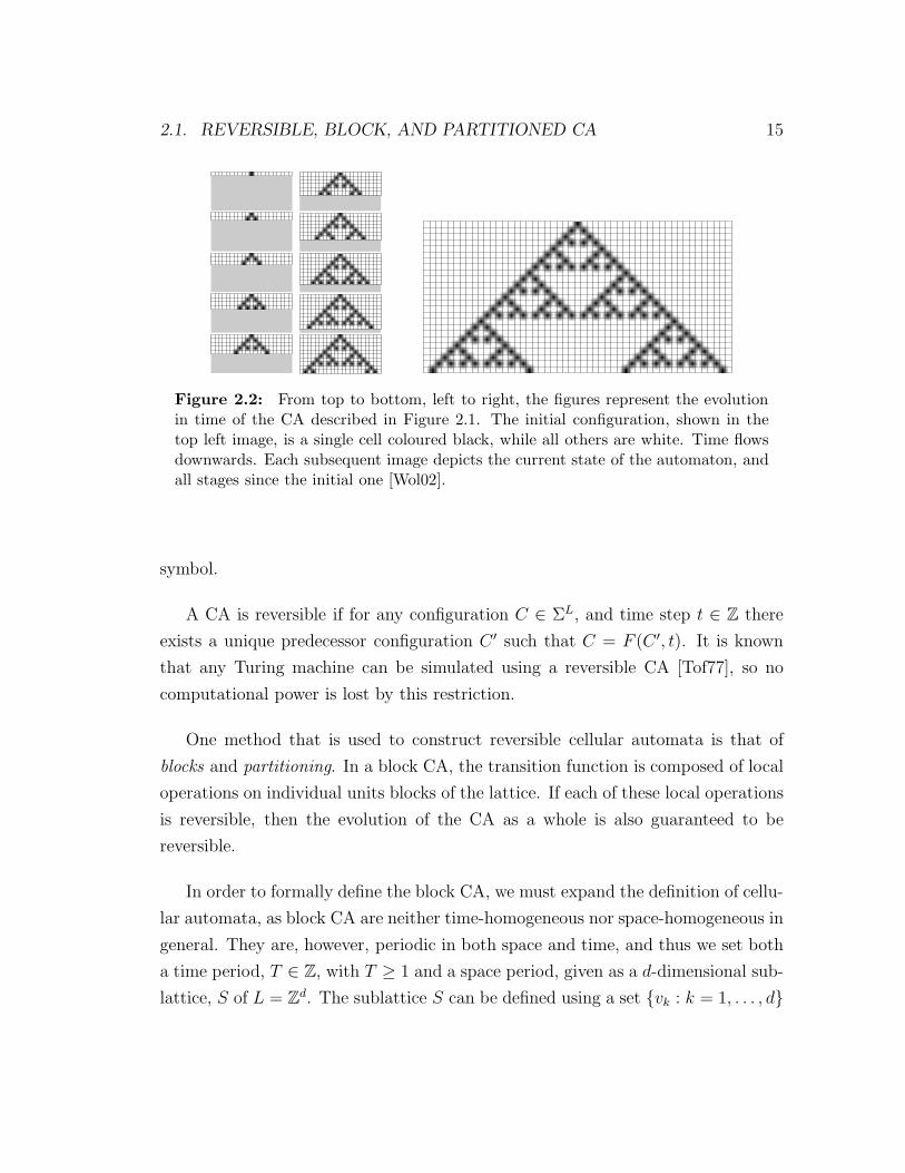
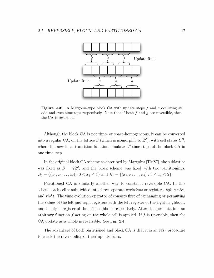
Figure 2.3: A Margolus-type block CA with update steps f and g occurring atodd and even timesteps respectively. Note that if both f and g are reversible, thenthe CA is reversible.
Although the block CA is not time- or space-homogeneous, it can be converted
into a regular CA, on the lattice S (which is isomorphic to Zd), with cell states ΣB,
where the new local transition function simulates T time steps of the block CA in
one time step.
In the original block CA scheme as described by Margolus [TM87], the sublattice
was fixed as S = 2Zd, and the block scheme was fixed with two partitionings:
B0 = (x1, x2 . . . , xd) : 0 ≤ xj ≤ 1 and B1 = (x1, x2 . . . , xd) : 1 ≤ xj ≤ 2.
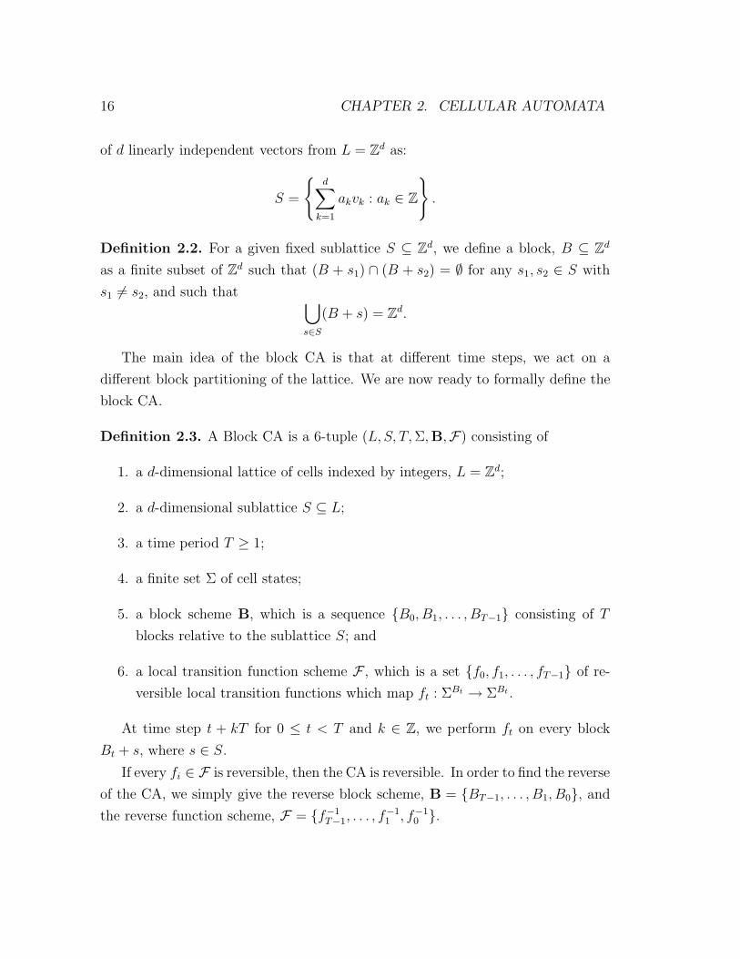
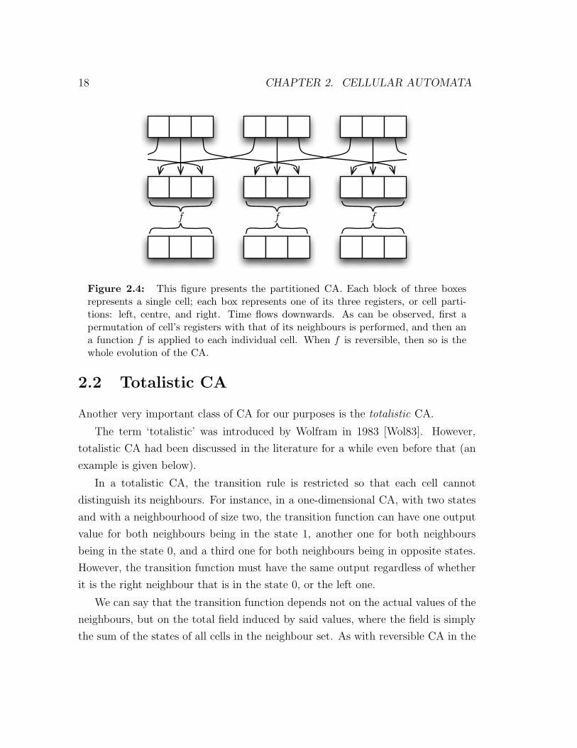
Partitioned CA is similarly another way to construct reversible CA. In this
scheme each cell is subdivided into three separate partitions or registers, left, centre,
and right. The time evolution operator of consists first of exchanging or permuting
the values of the left and right registers with the left register of the right neighbour,
and the right register of the left neighbour respectively. After this permutation, an
arbitrary function f acting on the whole cell is applied. If f is reversible, then the
CA update as a whole is reversible. See Fig. 2.4.
The advantage of both partitioned and block CA is that it is an easy procedure
to check the reversibility of their update rules.
18 CHAPTER 2. CELLULAR AUTOMATA
f f f
Figure 2.4: This figure presents the partitioned CA. Each block of three boxesrepresents a single cell; each box represents one of its three registers, or cell parti-tions: left, centre, and right. Time flows downwards. As can be observed, first apermutation of cell’s registers with that of its neighbours is performed, and then ana function f is applied to each individual cell. When f is reversible, then so is thewhole evolution of the CA.
2.2 Totalistic CA
Another very important class of CA for our purposes is the totalistic CA.
The term ‘totalistic’ was introduced by Wolfram in 1983 [Wol83]. However,
totalistic CA had been discussed in the literature for a while even before that (an
example is given below).
In a totalistic CA, the transition rule is restricted so that each cell cannot
distinguish its neighbours. For instance, in a one-dimensional CA, with two states
and with a neighbourhood of size two, the transition function can have one output
value for both neighbours being in the state 1, another one for both neighbours
being in the state 0, and a third one for both neighbours being in opposite states.
However, the transition function must have the same output regardless of whether
it is the right neighbour that is in the state 0, or the left one.
We can say that the transition function depends not on the actual values of the
neighbours, but on the total field induced by said values, where the field is simply
the sum of the states of all cells in the neighbour set. As with reversible CA in the
2.2. TOTALISTIC CA 19
previous section, it can be shown that putting such restriction on the transition
function do not limit its computational power (see below).
A very famous example of a totalisitc CA is Game of Life. Game of Life was
created by mathematician John Horton Conway in 1970. It is a 2D totalistic CA.
Each cell has two states: dead and alive. The transition function can be quite easily
described in plain English:
1. Any live cell with fewer than two live neighbours dies of loneliness.
2. Any live cell with more than three live neighbours dies by overcrowding.
3. Any live cell with two or three live neighbours lives, unchanged and happy,
to the next generation.
4. Any dead cell with exactly three live neighbours comes to life, thanks to
reproduction.
Although extremely simple, and seemingly limited due its totalistic rule, this
CA is extremely interesting. It can be shown, inter alia, that it is Turing complete.
Much study has gone into the many patterns that can evolve from such automata.
In general, classical CA are very interesting and powerful constructs, in their
elegance, simplicity, expressive powers, and even artistic beauty. A complete dis-
cussion of this field is beyond the scope of this chapter. Instead, we will turn to
the quantum analogue of this mathematical abstraction in the next chapter.

Chapter 3
Quantum Cellular Automata
In this chapter we will present the model of Quantum Cellular Automata that we
will use in this thesis. We call it the Local Unitary Quantum Cellular Automata
model because it is based on local unitary operators acting on qudits. We will
abbreviate this name to LUQCA, or just QCA when the context makes it clear we
are referring to the model herein presented.
In Chapter 4 we will show that our model is sound and complete. By complete-
ness we mean that LUQCA can achieve universal quantum computation. We will
show this by giving a QCA simulation of a quantum circuit.
By soundness we mean that the there exists an efficient simulation of every
QCA described in our model, by a quantum circuit. Formally, what we mean by
efficient simulation is that there exists a uniform family of quantum circuits that
can each simulate the evolution of a finite region of the QCA, for a specified number
of steps. Furthermore, we require that the depth of each circuit be linear in the
number of steps, and independent of the size of the region being simulated. This
last requirement is to ensure that the QCA retains the quintessential quality of CA:
massive parallelism.
The fact that there is such a guarantee, without any further restraints, is one of
the strongest virtues of the model herein presented. In Section 5 we will see that in
general, previous models cannot make such a guarantee. We will also discuss what
methods (if any) can be used to ensure efficient simulation in these models.
21
22 CHAPTER 3. QUANTUM CELLULAR AUTOMATA
3.1 Local Unitary QCA
Now, with a formal notion of CA, we can proceed to give a quantization. As
mentioned earlier, we will have very specific goals in mind.
3.1.1 Model Requirements
First, we want develop an intuitive model that is both simple to work with, and
to develop algorithms for. At the same time we want this model to be an obvious
extension of classical CA, and limit to classical CA behaviour under reasonable
assumptions.
Also, we want to keep our model grounded in physical realities. This has strong
consequences. Namely, we approach CA, even classical CA, not as abstract math-
ematical structures, but as models representing real physical systems.
A final, and perhaps more important consequence for quantum information sci-
entists, is that we expect our model to reliably describe quantum systems with
appropriate behaviour, acting as direct mathematical abstraction of these systems,
such as spin chains. An algorithm described in our model should be easily trans-
latable to an actual physical implementation on such quantum systems. We will
show in Chapter 8 that this is so.
3.1.2 A First Approach
The first step in our quantization of CA is to change the state space of a cell to
reflect a quantum system. There are several methods for doing so, however we
believe that the most natural way to approach this is to convert the alphabet of
the cellular automaton, Σ, into orthogonal basis states of a Hilbert space, HΣ.
Formally, every cell x ∈ L is assigned a qudit, |x〉 ∈ HΣ. This gives us a strong
intuitive tool, as the notion of a lattice of qudits should be familiar to anyone
working in quantum information theory.
It is also physically reasonable. As an example, spin chains can be directly
described by such mathematical constructions. Lattice gases, though not originally
3.1. LOCAL UNITARY QCA 23
modelled in this way, can also be easily described by such mathematical constructs.
Perhaps the most obvious physical example is the pulse-driven quantum computer.
We also wish to quantize the standard classical CA update rule. However, this
process cannot necessarily proceed in the most obvious manner. In a classical CA,
every cell is instantaneously updated in parallel. We wish to replace this classical
cell update rule with a quantum analogue that acts appropriately on the qudit
lattice described above. For a quantum unitary operation to act as a quantum cell
update rule, this operator needs to fulfill the following two restrictions:
1. The operator must act on a finite subset of the lattice. Precisely Ux :
H(Nx) → H(Nx) where Nx = N + x ⊆ L is the finite neighbourhood about
the cell x.
2. The operator must commute with lattice translations of itself. Precisely, we
require that [Ux, Uy] = 0 for all x, y ∈ Zn.
The first condition is an immediate condition for any rule, quantum or otherwise, to
qualify as a CA update rule. The second condition allows the operators Ux, x ∈ Zn
to be applied in parallel without the need to consider ordering of the operators, or
the need to apply them simultaneously.
It should be clear that any evolution defined in such manner represents a valid
quantum evolution which can be ascribed to some physical system. The global
evolution can be described as
U =∏
x
Ux,
whose action on the lattice is well-defined, due to the two conditions given above
(see Section 3.1.4).
The question that remains is whether this model properly describes what we
intuitively would regard as QCA. Properly, these are two questions:
1. Can all entities described by the model above be properly classified as QCA?
2. Can all systems that are identified as QCA be properly described in the model
above?
24 CHAPTER 3. QUANTUM CELLULAR AUTOMATA
The answer to the first question is yes, since the update rules are local and can be
applied in unison throughout the lattice. Also, the global unitary operator for the
evolution of the lattice properly defined, and is space-homogeneous, as desired.
The answer to the second question is, unfortunately, no. We present a simple
system that one might consider to be a valid QCA, but cannot be described in the
above model.
The counterexample is as follows. We start with a 1-dimensional lattice of
qudits. For each lattice cell x ∈ L, we associate with it a quantum state |ψx〉 ∈ HΣ.
Although in general, the configuration of a QCA may not be separable with respect
to each cell, the configuration can still be described in terms of a linear superposition
of these separable configurations. Thus, it suffices to consider such configurations.
At each time step we wish to have every value shifted one cell to the right. In
other words, after the first update each cell x should now store the state |ψx−1〉.After k steps each cell x should contain the state |ψx−k〉. In fact, such a transition
function cannot be implemented by any local unitary process.
To see why this is so, consider the most general procedure on the lattice imple-
mented using only local unitary operators. Such a procedure should take a finite
number of steps, say n. At each time step i, 1 ≤ i ≤ n, we may apply any series
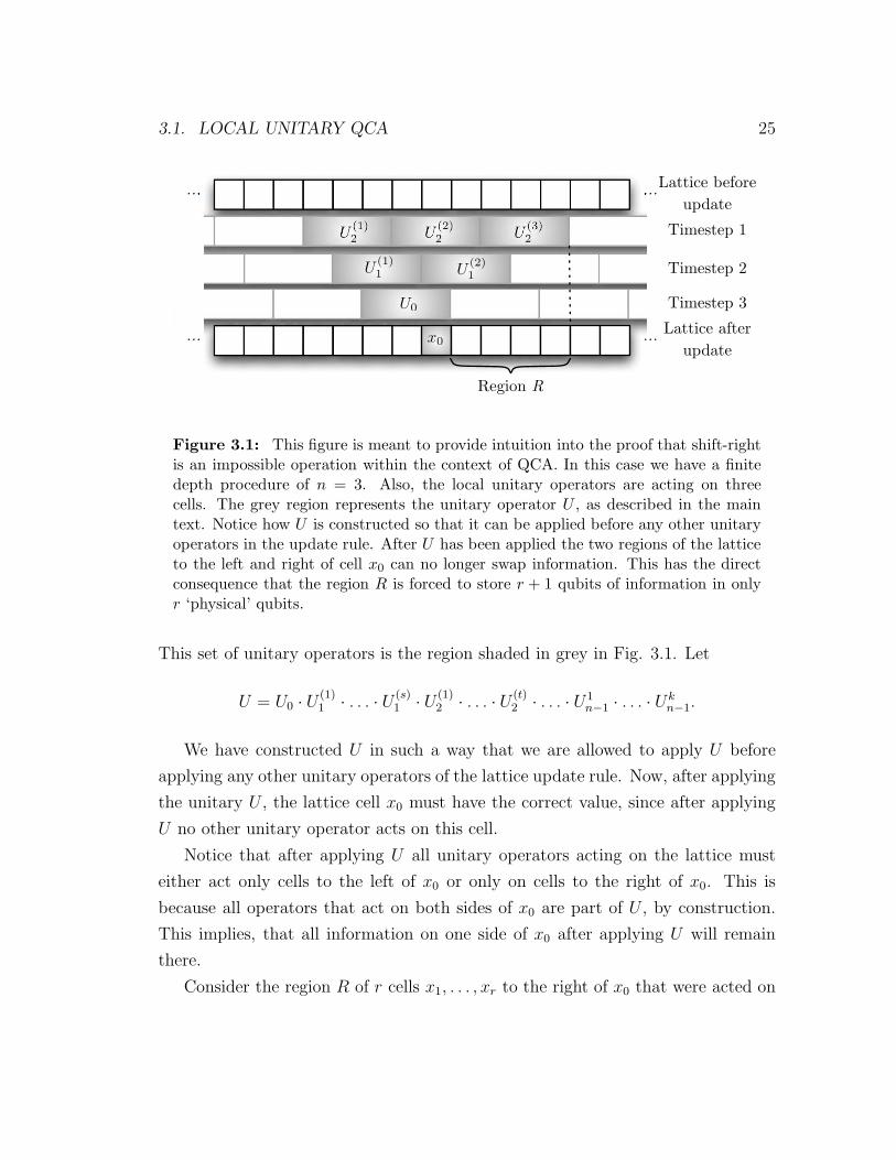
of unitary operators on disjoint sets of lattice points. See Fig. 3.1. In that figure
n = 3, and all the unitary operators act on sets of three lattice sites, but in general
both n and the size of the sets acted on by the unitary operators are arbitrary, and
not necessarily equal.
Suppose such a procedure implements the shift-right operation as described
above. Now, consider one particular lattice cell, call it x0. Now, we will construct
a unitary U . Consider the (only) unitary operator that acts on it in the n’th step.
Call this unitary U0. Now, consider all the lattice points that are acted upon by
U0, and take all the unitary operators that act on any of these lattice sites. Call
these unitary operators U(1)1 , . . . , U
(s)1 . Consider all the lattice acted upon by these
unitary operators, and all the unitary operators on step n− 2 that act upon these
sites. Call these operators U(1)2 , . . . , U
(t)2 , and so on, until reaching step 1 of the
update rule. In a sense we have constructed the past light cone of the cell site x0.
3.1. LOCAL UNITARY QCA 25
......
......
Lattice before
update
Lattice after
update
Timestep 1
Timestep 2
Timestep 3
Region R
Figure 3.1: This figure is meant to provide intuition into the proof that shift-rightis an impossible operation within the context of QCA. In this case we have a finitedepth procedure of n = 3. Also, the local unitary operators are acting on threecells. The grey region represents the unitary operator U , as described in the maintext. Notice how U is constructed so that it can be applied before any other unitaryoperators in the update rule. After U has been applied the two regions of the latticeto the left and right of cell x0 can no longer swap information. This has the directconsequence that the region R is forced to store r + 1 qubits of information in onlyr ‘physical’ qubits.
This set of unitary operators is the region shaded in grey in Fig. 3.1. Let
U = U0 · U (1)1 · . . . · U (s)
1 · U (1)2 · . . . · U (t)
2 · . . . · U1n−1 · . . . · Uk
n−1.
We have constructed U in such a way that we are allowed to apply U before
applying any other unitary operators of the lattice update rule. Now, after applying
the unitary U , the lattice cell x0 must have the correct value, since after applying
U no other unitary operator acts on this cell.
Notice that after applying U all unitary operators acting on the lattice must
either act only cells to the left of x0 or only on cells to the right of x0. This is
because all operators that act on both sides of x0 are part of U , by construction.
This implies, that all information on one side of x0 after applying U will remain
there.
Consider the region R of r cells x1, . . . , xr to the right of x0 that were acted on
26 CHAPTER 3. QUANTUM CELLULAR AUTOMATA
by U . Every cell, after the complete update rule has been applied, must contain
the state that was in the cell directly to the left of it before the update was applied.
This means that, after U has been applied, cell x0 contains what used to be in cell
x−1. Furthermore, the r cells in region R must contain the information that must
ultimately be in the r + 1 cells x1, . . . , xr+1. The information for these r + 1 cells
cannot be to the right of the cell xr because U did not affect any cells beyond cell
xr. Furthermore, if U stored this information to the left of the region r, there would
be no way to move it to the appropriate cells after U had been applied. Hence,
it is necessary for r qudits to store r + 1 qudits of information, which is clearly
impossible. A contradiction is arrived, and we conclude that it is impossible to
shift right all information in the lattice using only local unitary evolution.
While this argument is directed at infinite lattices, a similar argument holds
for finite—possibly cyclic—lattices. Here, clearly, the conclusion is not that it is
impossible to (cyclically) shift information, but rather that doing so requires a
complexity depth that is Ω(N) where N is the size of the lattice. This implies that
this is not a parallel operation, and hence not a cellular automata.
In order to resolve this issue, we need to analyse the classical CA parallel update
rules more closely. In the classical CA, the local update rule for a given cell reads the
value of the cell, and the values of its neighbouring cells. It performs a computation
based on these values, and then updates the cell’s value accordingly. Herein lies the
problem: read and update are modelled in a classical CA as a single atomic action
that can be applied throughout the lattice in parallel simultaneously. However, in
a physical setting, these two operations cannot be implemented in this manner.
When simulating CA in classical computer architectures, the canonical solution is
to use two lattices in memory: one to store the current value, and one to store the
computed updated value. Even if we consider hardware implementations of CA,
these need to keep the values of the inputs to the transition function while this
function is being calculated.
The formal CA model does not need to consider this implementation detail. It
can be argued that the classical CA tacitly calls for the information in each cell to
be cloned and stored, previous to each update rule.
3.1. LOCAL UNITARY QCA 27
However, due to the laws of quantum mechanics, we cannot take the same
liberties here.
3.1.3 A New Approach
We can now make an adjustment to our QCA model, given the importance of
maintaining independent read and update operations. Instead of having one unitary
operator replacing the single atomic operation in the CA model, we define our QCA
update rule as consisting of two unitary operators. The first operator, corresponding
to the read operation, will be as defined above: a unitary operator Ux, x ∈ L acting
on the neighbourhood Nx, which commutes with all lattice translations of itself,
Uy, y ∈ L. The second operator, Vx, x ∈ L, corresponds to the update operation,
and will only act on the single cell x itself.
The intuition is as follows: in our physical model, instead of having separate
lattices for the read and update functions, we expand each lattice cell to also con-
tain any space resources necessary for computing the updated value of the cell.
The operator Ux reads the values of the neighbourhood Nx, performs a computa-
tion, and stores the new value in such a way that does not prevent neighbouring
operators Uy from correctly reading its own input values. This allows each cell to
be operated upon independently, in parallel, without any underlying assumptions
of synchronization. After all the operations Ux have been performed, the second
unitary Vx performs the actual update of the lattice cell.
With this new model for the update operation, we can again approach the two
questions given above as to whether this model adequately describes what we might
intuitively regard as QCA.
First, it is clear that all entities described by this updated model can still be
properly classified as QCA. The local update rule Rx = VxUx is still a valid quantum
unitary operation, and the global update rule
R = V U =
(⊗
x
Vx
)(∏
x
Ux
)
28 CHAPTER 3. QUANTUM CELLULAR AUTOMATA
is space-homogeneous and has a well-defined action on the lattice.
Now, in order to properly investigate whether all physical systems which can be
described as QCA can be described within this new model, it is necessary to verify
the following:
We must first compare our model to existing CA models, both classical and
quantum, in order to ensure that our model subsumes all proper CA described
in these models. Secondly, we must also show that any known physical system
which behaves according to quantum mechanics and satisfies the CA preconditions
of being driven by a local, space-homogeneous interaction can be described by our
model.
As an example, the qubit shift-right QCA mentioned above can now be described
in this model, by including ancillary computation space with each lattice cell.
We will tackle this question in more depth in the upcoming sections. First, we
present a formal definition of the QCA model which we will adopt, as described in
this section.
Definition 3.1 (QCA). A Quantum Cellular Automaton is a 5-tuple (L,Σ,N , U0, V0)
consisting of:
1. a d-dimensional lattice of cells indexed by integers, L = Zd,
2. a finite set Σ of orthogonal basis states,
3. a finite neighbourhood scheme N ⊆ Zd that includes the point at the origin,
4. a local read function U0 ∈ U (HΣ)⊗N , and
5. a local update function V0 ∈ U(HΣ).
The read operation carries the further restriction that any two lattice translations
Ux and Uy must commute for all x, y ∈ L.
Each cell has a finite Hilbert space associated with it HΣ = span (|σ〉σ∈Σ).
The reduced state of each cell x ∈ L is a density operator over this Hilbert space
ρx ∈ D (HΣ).
3.1. LOCAL UNITARY QCA 29
The initial state of the QCA is defined in the following way. Let f be any
computable function that maps lattice vectors to pure quantum states in (HΣ)⊗kd
,
where d is the dimension of the QCA lattice, and k is the block size of the ini-
tial state. Then for any lattice vector z = (z1k, z2k, . . . , zdk) ∈ Zd the initial
state of the lattice hypercube delimited by (z1k, z2k, . . . , zdk) and ((z1 + 1)k − 1,
(z2 + 1)k − 1, . . . , (zd + 1)k − 1) is set to f(z).
In particular f can have a block size of one cell, initializing every cell in a region
to the same state in Σ. It can also have more complicated forms like initializing
pairs of cells in a one dimensional QCA to some maximally entangled state. Finally,
we require that every f initialize all but a finite set of cells to a some quiescent
state (see next section).
The local update rule acting on a cell x consists of the operation Ux followed
by the single-cell operation Vx, where Ux (Vx) is simply the appropriate lattice
translation of U0 (V0). The global evolution operator R is as previously defined.
3.1.4 Quiescent States
Our QCA definition follows the classical CA convention in defining the model over
an infinite lattice. However, we will often be concerned only with finite regions
of the QCA. For example, any physical implementation of a QCA using quantum
hardware will, by necessity, simulate only a finite region of the QCA. Another
reason is for simulating physical phenomena. For instance, in Chapter 7, we will
be interested in simulating finite size chains of spin-12
particles.
Sometimes, it can be appropriate to simply use finite QCA with cyclic boundary
conditions. In this case, we envision the lattice as a closed torus. This is a standard
and well-known practice with CA. For example, we can use this technique if the
spin chain we wish to simulate is closed, that is, it itself wraps around. For other
applications, this will not be appropriate, for example, when trying to simulate an
open spin chain, which is a chain that does not wrap around, but rather has two
distinct end points. Another example will be the spin-signal amplification algorithm
in Chapter 9, which uses a finite size cube ancilla system.
In such cases, the most appropriate way to proceed is to make use of a quiescent
30 CHAPTER 3. QUANTUM CELLULAR AUTOMATA
state. A quiescent state |e〉 for a QCA with update operators U0 ∈ U (HΣ)⊗N , and
V0 ∈ U (HΣ), is such that
1. Vx |e〉 = |e〉
2. Ux
(|e〉⊗N
)= |e〉⊗N
3. For all cells y in the neighbourhood of x other than the cell x itself,
trHN (x)\HyU0 (|ey〉 〈ey| ⊗ ρ)U †
0 = |ey〉 〈ey| ,
where HN (x) is the Hilbert space of the neighbourhood of x and Hy is the
Hilbert space of the cell y.
In simple terms, what rules 1 and 2 say is that the the update rule of a cell
is not allowed to move that cell out of a quiescent state if all its neighbours are
also quiescent. Rule 3 adds the constraint that the update rule of a cell y is never
allowed to move a cell x 6= y out of a quiescent state. Together, these rules ensure
that our notion of quiescent is the same as that for classical cellular automata.
Namely, that a cell that is in a quiescent state, and whose neighbours are all also
in that quiescent state at time step t, will remain quiescent at time step t+ 1.
It may seem that the definition is very restrictive on what type of update op-
erators U0 and V0 admit quiescent states. This is not the case. Any unitary V
and lattice commuting unitary U of some QCA Q can be made to accommodate a
quiescent state by simply extending the alphabet of Q with a quiescent state, and
setting U0 and V0 to act trivially on this state.
As an example, in the case of the finite spin-12
chains, we can use three state
cells. We use the state labels |+1〉 and |−1〉 to refer to the presence of a spin-12
particle in a given cell position in the states 12(1l + σz) and 1
2(1l − σz) respectively.
A third state, labelled |0〉 denotes the absence of any particle in that cell location.
One needs then only ensure that the update rule correctly acts on states |+1〉 and
|−1〉, while leaving state |0〉 unaffected.
Quiescent states are also very useful for the purposes of simulation, and physical
implementation. Normally, if one is interested in the state of a region S of the lattice
3.1. LOCAL UNITARY QCA 31
Trace out Trace out
Unitary Evolution
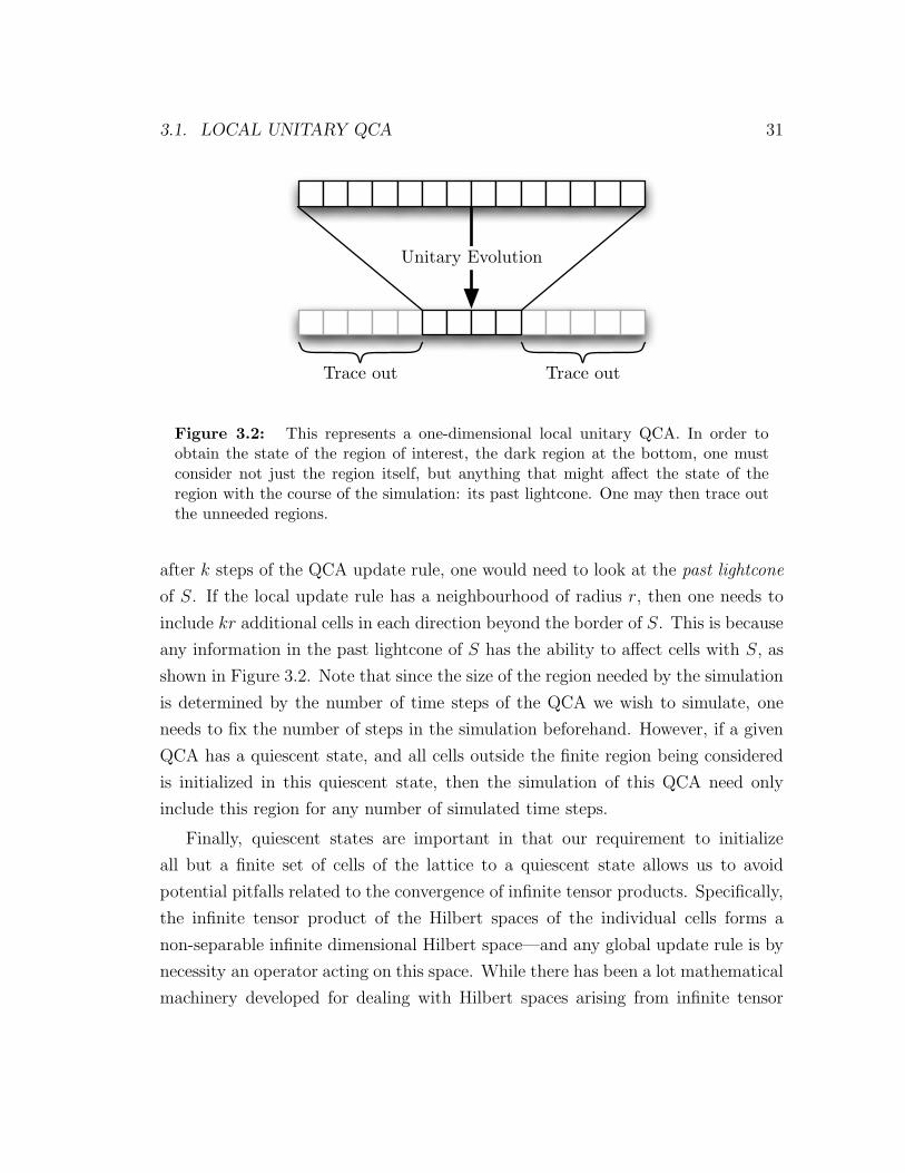
Figure 3.2: This represents a one-dimensional local unitary QCA. In order toobtain the state of the region of interest, the dark region at the bottom, one mustconsider not just the region itself, but anything that might affect the state of theregion with the course of the simulation: its past lightcone. One may then trace outthe unneeded regions.
after k steps of the QCA update rule, one would need to look at the past lightcone
of S. If the local update rule has a neighbourhood of radius r, then one needs to
include kr additional cells in each direction beyond the border of S. This is because
any information in the past lightcone of S has the ability to affect cells with S, as
shown in Figure 3.2. Note that since the size of the region needed by the simulation
is determined by the number of time steps of the QCA we wish to simulate, one
needs to fix the number of steps in the simulation beforehand. However, if a given
QCA has a quiescent state, and all cells outside the finite region being considered
is initialized in this quiescent state, then the simulation of this QCA need only
include this region for any number of simulated time steps.
Finally, quiescent states are important in that our requirement to initialize
all but a finite set of cells of the lattice to a quiescent state allows us to avoid
potential pitfalls related to the convergence of infinite tensor products. Specifically,
the infinite tensor product of the Hilbert spaces of the individual cells forms a
non-separable infinite dimensional Hilbert space—and any global update rule is by
necessity an operator acting on this space. While there has been a lot mathematical
machinery developed for dealing with Hilbert spaces arising from infinite tensor
32 CHAPTER 3. QUANTUM CELLULAR AUTOMATA
product of finite spaces [Thi83], we can completely sidestep the issue, by restricting
our attention to initial states with only finitely many non-quiescent states. First,
we can always restrict our attention to the subspace of the lattice that is the tensor
of all lattice points with non-quiescent states, and those lattice points in their
neighbourhoods. This is always a finite-dimensional Hilbert space. Then, the
global operator U can be now properly defined as an operator acting on this finite
dimensional Hilbert space.
There are three important observations regarding this approach. First, this
does not limit the computation power of the QCA model. In particular, this does
not imply that this is a bounded computation model. The set of cells in non-
quiescent states can increase as time moves forward. This does imply that the
global operator U can act on increasingly larger spaces, as times goes on. This
is in not a problem, as U can always be extended uniquely to the larger space,
by appropriately using the local update functions U0 and V0. Finally, while it
may be possible and theoretically interesting to do away with this quiescent state
requirement, there is little motivation to do so in terms of computational and
physical simulation applications, which is our prime interest in this thesis.
Chapter 4
Quantum Circuits and
Universality
In this chapter we explore two important aspects of the QCA model we introduced
in Section 3.1. These aspects relate to QCA as a model of computation. First,
it is important to show that QCA are capable of universal quantum computation.
We demonstrate this using a simulation of an arbitrary quantum circuit using a
2-dimensional QCA.
We also show that any QCA can be simulated using families of quantum circuits.
A quantum circuit is defined as a finite set of gates acting on a finite input. One can
then define a uniform family of quantum circuits, with parameters S and t, such
that each circuit simulates the finite region S of the QCA for t update steps. By
uniformity we mean that that there exists an effective procedure, such as a Turing
machine, that on input (S, t) outputs the correct circuit.
We will show that our simulation is efficient, as defined previously. Specifically,
in order to simulate a QCA on a given region, for a fixed number of time steps, we
give a quantum circuit simulation with a depth which is linear with respect to the
number of time steps, and independent of the size of the simulated region.
33
34 CHAPTER 4. QUANTUM CIRCUITS AND UNIVERSALITY
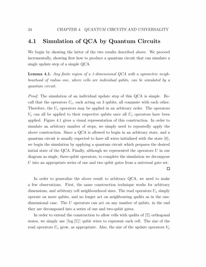
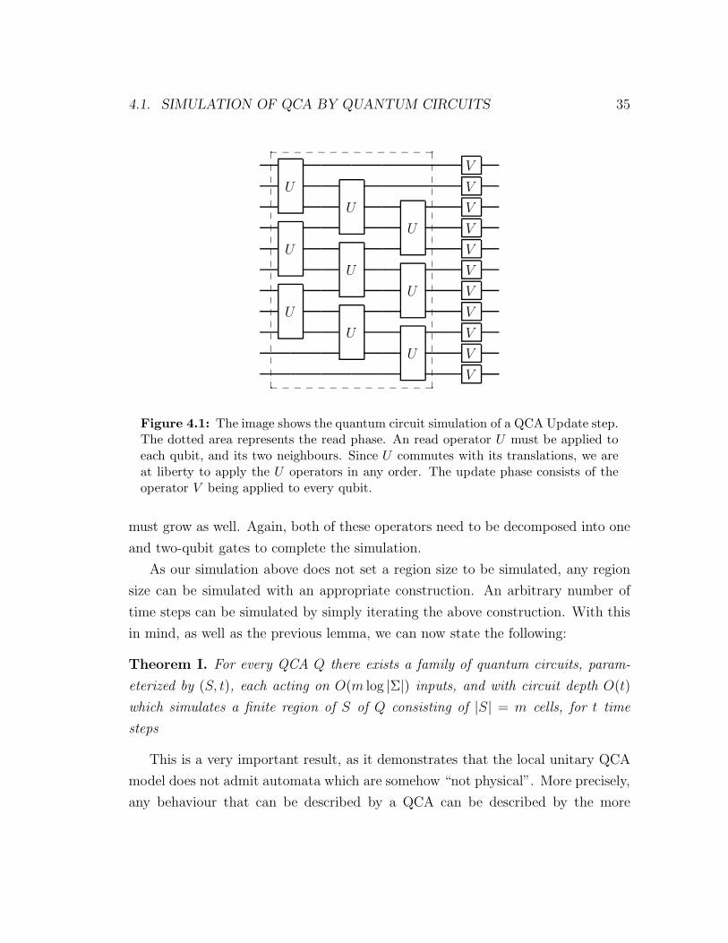
4.1 Simulation of QCA by Quantum Circuits
We begin by showing the latter of the two results described above. We proceed
incrementally, showing first how to produce a quantum circuit that can simulate a
single update step of a simple QCA.
Lemma 4.1. Any finite region of a 1-dimensional QCA with a symmetric neigh-
bourhood of radius one, where cells are individual qubits, can be simulated by a
quantum circuit.
Proof. The simulation of an individual update step of this QCA is simple. Re-
call that the operators Ux, each acting on 3 qubits, all commute with each other.
Therefore, the Ux operators may be applied in an arbitrary order. The operators
Vx can all be applied to their respective qubits once all Ux operators have been
applied. Figure 4.1 gives a visual representation of this construction. In order to
simulate an arbitrary number of steps, we simply need to repeatedly apply the
above construction. Since a QCA is allowed to begin in an arbitrary state, and a
quantum circuit is usually expected to have all wires initialized with the state |0〉,we begin the simulation by applying a quantum circuit which prepares the desired
initial state of the QCA. Finally, although we represented the operators U in our
diagram as single, three-qubit operators, to complete the simulation we decompose
U into an appropriate series of one and two qubit gates from a universal gate set.
In order to generalize the above result to arbitrary QCA, we need to make
a few observations. First, the same construction technique works for arbitrary
dimensions, and arbitrary cell neighbourhood sizes. The read operators Ux simply
operate on more qubits, and no longer act on neighbouring qudits as in the one-
dimensional case. The U operators can act on any number of qubits, in the end
they are decomposed into a series of one and two-qubit gates.
In order to extend the construction to allow cells with qudits of |Σ| orthogonal
states, we simply use ⌈log |Σ|⌉ qubit wires to represent each cell. The size of the
read operators Ux grow, as appropriate. Also, the size of the update operators Vx
4.1. SIMULATION OF QCA BY QUANTUM CIRCUITS 35
U
V
U
V
U
V
U
V
U
V
U
V
U
V
U
V
U
V
V
V
_ _ _ _ _ _ _ _ _ _ _ _ _ _
_ _ _ _ _ _ _ _ _ _ _ _ _ _
Figure 4.1: The image shows the quantum circuit simulation of a QCA Update step.The dotted area represents the read phase. An read operator U must be applied toeach qubit, and its two neighbours. Since U commutes with its translations, we areat liberty to apply the U operators in any order. The update phase consists of theoperator V being applied to every qubit.
must grow as well. Again, both of these operators need to be decomposed into one
and two-qubit gates to complete the simulation.
As our simulation above does not set a region size to be simulated, any region
size can be simulated with an appropriate construction. An arbitrary number of
time steps can be simulated by simply iterating the above construction. With this
in mind, as well as the previous lemma, we can now state the following:
Theorem I. For every QCA Q there exists a family of quantum circuits, param-
eterized by (S, t), each acting on O(m log |Σ|) inputs, and with circuit depth O(t)
which simulates a finite region of S of Q consisting of |S| = m cells, for t time
steps
This is a very important result, as it demonstrates that the local unitary QCA
model does not admit automata which are somehow “not physical”. More precisely,
any behaviour that can be described by a QCA can be described by the more
36 CHAPTER 4. QUANTUM CIRCUITS AND UNIVERSALITY
traditional quantum circuit model. Furthermore, such descriptions retain the high
parallelism inherent to QCA.
4.2 Simulation of Quantum Circuits by QCA
Next, we show the converse result from the one above, thus showing that local
unitary QCA are capable of efficient universal quantum computation.
Theorem II. There exists a universal QCA Qu that can simulate any quantum
circuit by using an appropriately encoded initial state.
Proof. We proceed by constructing the QCA Qu over a 2-dimensional lattice. We
will basically ‘draw’ the circuit onto the lattice. The qubits will be arranged top
to bottom, and the wires will be visualized as going from left to right.
Each cell will consist of a number of fields, or registers. The cell itself can
be thought of as the tensor product of quantum systems corresponding to these
registers. The first register, the State register, consists of a single qubit which
corresponds directly to the value on one of the wires of the quantum circuit at a
particular point in the computation. This value will be shifted towards the right
as time moves forward. Next is the Gate register. This register will be initialized
to a value corresponding to a gate that is to be applied to the state register, at
the appropriate time. There is a clock register, which will keep track the current
time step of the simulation. This clock register is in reality just a qubit, and keeps
track of which of the two phases we are currently in. There are two phases to
the simulation, an ‘operate’ and a ‘carry’. There is finally a single qubit Active
register, that keeps a record of which cells are currently actively involved in the
computation. This register is either set to true or false.
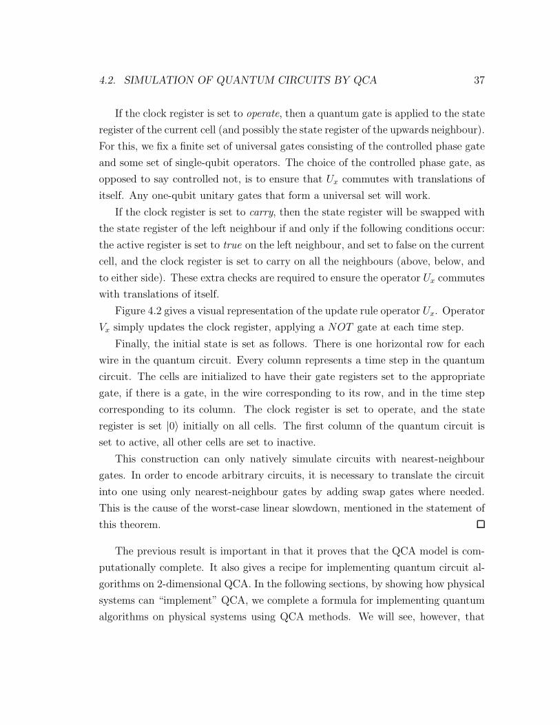
The local read operator Ux proceeds as follows. The neighbourhood scheme
is the von Neumann neighbourhood of radius one, i.e. the cells directly above,
below and to either side of the cell. The read operator acts non-trivially only on
the one cell directly above, and the one directly to the left. However, the bigger
neighbourhood is needed to ensure unitary evolution, and translation invariance.
4.2. SIMULATION OF QUANTUM CIRCUITS BY QCA 37
If the clock register is set to operate, then a quantum gate is applied to the state
register of the current cell (and possibly the state register of the upwards neighbour).
For this, we fix a finite set of universal gates consisting of the controlled phase gate
and some set of single-qubit operators. The choice of the controlled phase gate, as
opposed to say controlled not, is to ensure that Ux commutes with translations of
itself. Any one-qubit unitary gates that form a universal set will work.
If the clock register is set to carry, then the state register will be swapped with
the state register of the left neighbour if and only if the following conditions occur:
the active register is set to true on the left neighbour, and set to false on the current
cell, and the clock register is set to carry on all the neighbours (above, below, and
to either side). These extra checks are required to ensure the operator Ux commutes
with translations of itself.
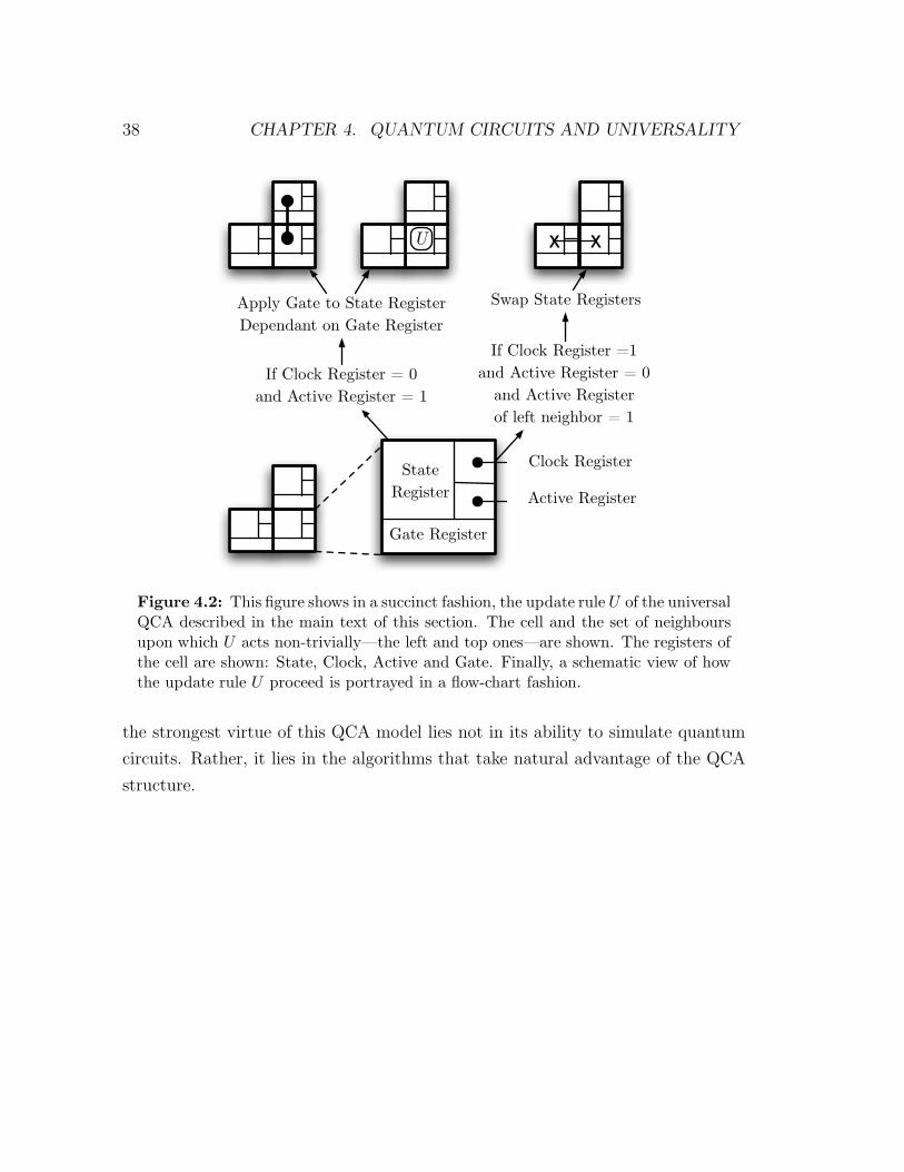
Figure 4.2 gives a visual representation of the update rule operator Ux. Operator
Vx simply updates the clock register, applying a NOT gate at each time step.
Finally, the initial state is set as follows. There is one horizontal row for each
wire in the quantum circuit. Every column represents a time step in the quantum
circuit. The cells are initialized to have their gate registers set to the appropriate
gate, if there is a gate, in the wire corresponding to its row, and in the time step
corresponding to its column. The clock register is set to operate, and the state
register is set |0〉 initially on all cells. The first column of the quantum circuit is
set to active, all other cells are set to inactive.
This construction can only natively simulate circuits with nearest-neighbour
gates. In order to encode arbitrary circuits, it is necessary to translate the circuit
into one using only nearest-neighbour gates by adding swap gates where needed.
This is the cause of the worst-case linear slowdown, mentioned in the statement of
this theorem.
The previous result is important in that it proves that the QCA model is com-
putationally complete. It also gives a recipe for implementing quantum circuit al-
gorithms on 2-dimensional QCA. In the following sections, by showing how physical
systems can “implement” QCA, we complete a formula for implementing quantum
algorithms on physical systems using QCA methods. We will see, however, that
38 CHAPTER 4. QUANTUM CIRCUITS AND UNIVERSALITY
Clock Register
Active Register
Gate Register
State
Register
If Clock Register = 0
and Active Register = 1
Apply Gate to State Register
Dependant on Gate Register
If Clock Register =1
and Active Register = 0
and Active Register
of left neighbor = 1
Swap State Registers
X XU
Figure 4.2: This figure shows in a succinct fashion, the update rule U of the universalQCA described in the main text of this section. The cell and the set of neighboursupon which U acts non-trivially—the left and top ones—are shown. The registers ofthe cell are shown: State, Clock, Active and Gate. Finally, a schematic view of howthe update rule U proceed is portrayed in a flow-chart fashion.
the strongest virtue of this QCA model lies not in its ability to simulate quantum
circuits. Rather, it lies in the algorithms that take natural advantage of the QCA
structure.
Chapter 5
Previous QCA Models
In this chapter, we will present a number of other models of QCA that have been
developed, and we will relate them to our proposed model.
5.1 Watrous-van Dam QCA
The first attempt to define a quantized version of cellular automata was made by
Watrous [Wat95], whose ideas were further explored by van Dam [vD96], and by
Durr, LeThanh and Santha [DS96,DLS97]. The model considers a one-dimensional
lattice of cells and a finite set of basis states Σ for each individual cell, and features
a transition function which maps a neighbourhood of cells to a single quantum state
instantaneously and simultaneously. Watrous also introduces a model of partitioned
QCA in which each cell contains a triplet of quantum states, and a permutation is
applied to each cell neighbourhood before the transition function is applied.
Formally, a Watrous-van Dam QCA, acting on a one-dimensional lattice indexed
by Z, consists of a 3-tuple (Σ,N , f) consisting of a finite set Σ of cell states, a finite
neighbourhood scheme N , and a local transition function f : ΣN → HΣ.
This model can be viewed as a direct quantization of the classical cellular au-
tomata model, where the set of possible configurations of the CA is extended to
include all linear superpositions of the classical cell configurations, and the local
transition function now maps the cell configurations of a given neighbourhood to
39
40 CHAPTER 5. PREVIOUS QCA MODELS
a quantum state. In the case that a neighbourhood is in a linear superposition of
configurations, f simply acts linearly. Also note that in this model, at each time
step, each cell is updated with its new value simultaneously, as in the classical
model.
Unfortunately, this definition allows for non-physical behaviour. It is possible to
define transition functions which do not represent unitary evolution of the cell tape,
either by producing superpositions of configurations which do not have norm 1, or
by not being injective, giving configurations which are not reachable by evolution
from some other configuration. In order to help resolve this problem, Watrous
restricts the set of permissible local transition functions by introducing the notion
of well-formed QCA. A local transition function is well-formed simply if it maps
any configuration to a properly normalized linear superposition of configurations.
Because the set of configurations is infinite, this condition is usually expressed in
terms of the ℓ2 norm of the complex amplitudes associated with each configuration.
In order to describe QCA which undergo unitary evolution, Watrous also intro-
duces the idea of a quiescent state, which is a distinguished element ǫ ∈ Σ which
has the property that f : ǫN 7→ ǫN . We can then define a quiescent QCA as a
QCA with a distinguished quiescent state which acts only on finite configurations,
which are configurations consisting of finitely many non-quiescent states. It can be
shown that a quiescent QCA which is well-formed and injective represents unitary
evolution on the lattice. Also, note that this notion of a quiescent state is slightly
different than the one introduced in Section 3.1.
Given the difficulty of ascertaining the well-formedness of general Watrous-van
Dam QCA [DS96,DLS97,Wat95] Watrous also introduces a model of partitioned
QCA, or PQCA.
A PQCA Qp is a tuple (Σ,N , f) where Σ and f are further constrained. In
this model each cell consists of three quantum states, so that the set of finite states
can be subdivided as Σ = Σl × Σc × Σr. Given a configuration in which each cell,
indexed by k ∈ Z, is in the state (q(l)k , q
(c)k , q
(r)k ), the transition function of the PQCA
consists first of a permutation which brings the state of cell k to (q(l)k−1, q
(c)k , q
(r)k+1) for
each k ∈ Z, then performs a local update function f ∈ U (HΣ) on each cell. Notice
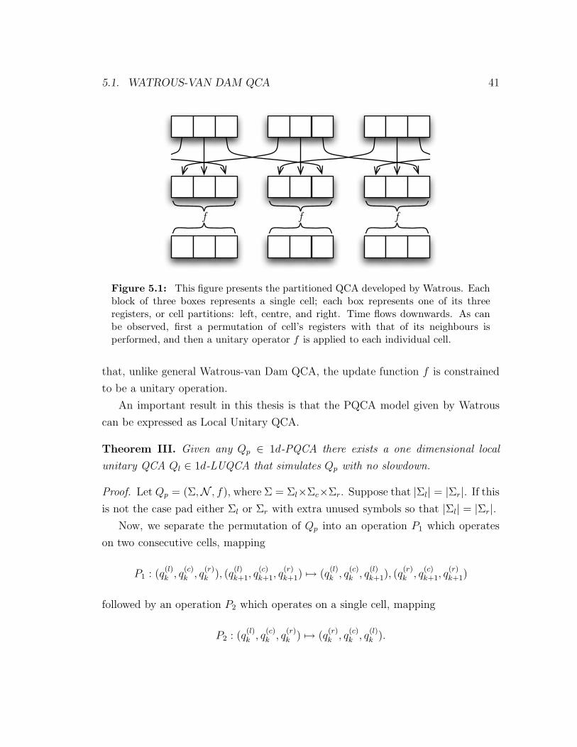
5.1. WATROUS-VAN DAM QCA 41
f f f
Figure 5.1: This figure presents the partitioned QCA developed by Watrous. Eachblock of three boxes represents a single cell; each box represents one of its threeregisters, or cell partitions: left, centre, and right. Time flows downwards. As canbe observed, first a permutation of cell’s registers with that of its neighbours isperformed, and then a unitary operator f is applied to each individual cell.
that, unlike general Watrous-van Dam QCA, the update function f is constrained
to be a unitary operation.
An important result in this thesis is that the PQCA model given by Watrous
can be expressed as Local Unitary QCA.
Theorem III. Given any Qp ∈ 1d-PQCA there exists a one dimensional local
unitary QCA Ql ∈ 1d-LUQCA that simulates Qp with no slowdown.
Proof. Let Qp = (Σ,N , f), where Σ = Σl×Σc×Σr. Suppose that |Σl| = |Σr|. If this
is not the case pad either Σl or Σr with extra unused symbols so that |Σl| = |Σr|.Now, we separate the permutation of Qp into an operation P1 which operates
on two consecutive cells, mapping
P1 : (q(l)k , q
(c)k , q
(r)k ), (q
(l)k+1, q
(c)k+1, q
(r)k+1) 7→ (q
(l)k , q
(c)k , q
(l)k+1), (q
(r)k , q
(c)k+1, q
(r)k+1)
followed by an operation P2 which operates on a single cell, mapping
P2 : (q(l)k , q
(c)k , q
(r)k ) 7→ (q
(r)k , q
(c)k , q
(l)k ).
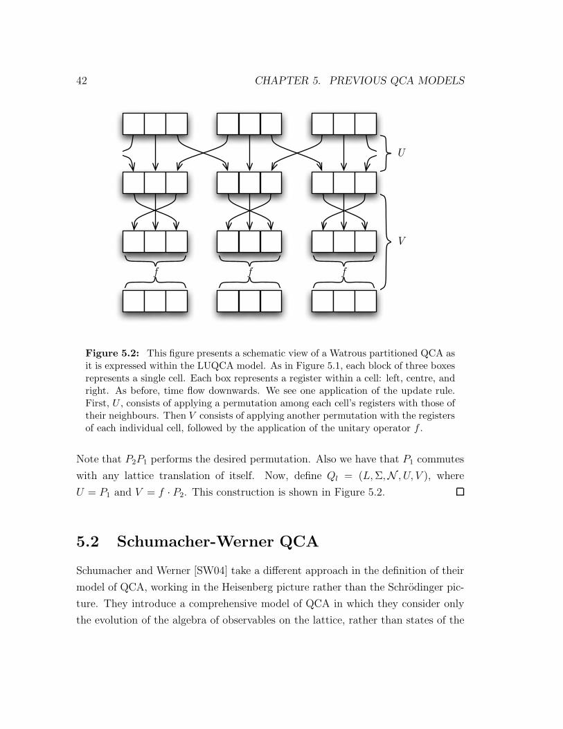
42 CHAPTER 5. PREVIOUS QCA MODELS
U
V
f f f
Figure 5.2: This figure presents a schematic view of a Watrous partitioned QCA asit is expressed within the LUQCA model. As in Figure 5.1, each block of three boxesrepresents a single cell. Each box represents a register within a cell: left, centre, andright. As before, time flow downwards. We see one application of the update rule.First, U , consists of applying a permutation among each cell’s registers with those oftheir neighbours. Then V consists of applying another permutation with the registersof each individual cell, followed by the application of the unitary operator f .
Note that P2P1 performs the desired permutation. Also we have that P1 commutes
with any lattice translation of itself. Now, define Ql = (L,Σ,N , U, V ), where
U = P1 and V = f · P2. This construction is shown in Figure 5.2.
5.2 Schumacher-Werner QCA
Schumacher and Werner [SW04] take a different approach in the definition of their
model of QCA, working in the Heisenberg picture rather than the Schrodinger pic-
ture. They introduce a comprehensive model of QCA in which they consider only
the evolution of the algebra of observables on the lattice, rather than states of the
5.2. SCHUMACHER-WERNER QCA 43
cell lattice itself. By extending local observables of the cell lattice into an closed
observable algebra, the Schumacher-Werner model has a number of useful algebraic
properties. In this model, the transition function is simply a homomorphism of the
observable algebra which satisfies a locality condition. Schumacher and Werner also
introduce a model of partitioned QCA called the Generalized Margolus Partitioned
QCA, in which the observable algebra is partitioned into subalgebras. This gener-
alizes the Margolus scheme, previously described, in which the cell lattice itself is
partitioned.
In order to avoid problematic issues dealing with observables over an infinite
lattices, Schumacher and Werner make use of the quasi-local algebra. In order to
construct this algebra, we first start with the set of all observables on finite subsets
S ⊆ L of the lattice, denoted A(S), and extend them appropriately into observables
of the entire lattice by taking a tensor product with the identity operator over the
rest of the lattice. The completion of this set forms the quasi-local algebra.
In this setting, the global transition operator of a QCA is simply defined as a ho-
momorphism T : A(L) → A(L) over the quasi-local algebra which satisfies two spe-
cific properties. First, a locality condition must be satisfied: T (A(S)) ⊆ A(S+N )
for all finite S ⊆ L. Secondly, T must commute with lattice translation operators,
so that the QCA is space-homogeneous. Now, the QCA can be defined in terms of
the lattice L, the neighbourhood scheme N , the single-cell observable algebra, A0,
which takes the place of the alphabet, and the global transition operator T .
The local transition operator of a QCA is simply a homomorphism T0 : A0 →A(N ) from the observable algebra of a single distinguished cell 0 ∈ L to the ob-
servable algebra of the neighbourhood of that cell. Schumacher and Werner show
that a local homomorphism T0 will correspond uniquely to a global transition oper-
ator T if and only if for each x ∈ L, the algebras T0(A0) and τx(T0(A0)) commute
element-wise. Here, τx is a lattice translation by x. The global transition operator
T given by T0 is defined by
T (A(S)) =∏
x∈S
Tx(Ax).
44 CHAPTER 5. PREVIOUS QCA MODELS
Next, we will describe the Generalized Margolus Partitioned QCA. Schumacher
and Werner present this model as a method of producing valid reversible QCA
in their model. In order to describe this model, we will proceed according to the
definition of a classical partitioned CA, as given in Chapter 2.
We start with the d-dimensional lattice L = Zd, and we fix the sublattice
S = 2Zd as the set of cells of L with all even co-ordinates. We also fix the time
period as T = 2. The block scheme, B is simply B0, B1. Where B0 is defined as
B0 = (x1, x2, . . . , xd) ∈ L : 0 ≤ xj ≤ 1, 1 ≤ j ≤ d,
which is simply a cube of size 2d with corners at cells 0 = (0, 0, . . . , 0) and 1 =
(1, 1, . . . , 1); and B1 is defined similarly as
B1 = B0 + 1,
which is simply a translation of the cube B0.
Now, as in the regular Schumacher-Werner QCA model, we proceed in the
Heisenberg picture. For any block B0 + s, s ∈ S, we have 2d intersecting blocks
from the partition B1 + S. For each block B1 + s′ which intersects with B0 + s,
there is a vector v ∈ Zd representing the translation taking B0 + s to B1 + s′, so
that B1 + s′ = B0 + s+ v. Indeed, these 2d intersecting blocks may be indexed by
the vectors v, which are simply all vectors of Zd whose entries are each ±1. Hence,
we will set B(s)v = B0 + s+ v.
For each block B(0)v , we will fix an observable algebra B(0)
v as a subalgebra of
the observable algebra A(B(0)v ) for the entire block. Then, for each block B
(s)v , the
observable algebra B(s)v is simply the appropriate translation of B(0)
v . Note that, in
particular, the observable algebra for the block B1 + s = B(s)1
, A(B(s)1
), contains
each of the observable algebras B(s+1−v)v . In order for an assignment of subalgebras
to be considered valid, these subalgebras B(s+1−v)v must commute and span A(B
(s)1
).
This occurs if and only if the product of the dimensions of these algebras is |Σ|2d
.
5.2. SCHUMACHER-WERNER QCA 45
The transition function then consists first of a isomorphism
T(s)0 : A(B
(s)0
) →∏
v
B(s)v ,
followed by the isomorphism
T(s)1 :
∏
v
B(s+1−v)v → A(B
(s)1
).
Note that since T0 and T1 are isomorphisms between observable algebras of equal
dimension, with an appropriate choice of basis, they can be represented by unitary
operators U0 and U1 which map vectors from a complex vector space to another
complex vector space of equal dimension. However, they do not represent local uni-
tary evolution, since these complex vector spaces are used to describe two different
quantum systems.
For example, the Shift-Right QCA, which was shown in Section 3.1 to not
be implementable using only local unitary operations, can be constructed in the
Generalized Margolus Partitioning QCA model. A consequence of this, inter alia, is
that there exist Schumacher-Werner QCA that cannot be implemented as quantum
circuits using the approach used in Chapter 4.
However, it is possible to implement the Generalized Margolus Partitioning
QCA model within the Local Unitary QCA model:
Theorem IV. Given a QCA Qs in the Werner-Schumacher Generalized Margolus
QCA model, there exists an LUQCA Ql that simulates it with at most constant
slowdown.
Proof. We start by adding 2d memory registers to each cell corresponding to the
subalgebras Bv in addition to a clock register indicating which of the two stages
of the transition function is being performed. The transition function of the Local
Unitary QCA simply swaps the contents of the data registers of each cell with the
appropriate memory registers before applying the unitary operations corresponding
to the desired isomorphisms.
46 CHAPTER 5. PREVIOUS QCA MODELS
5.3 Other Models
Meyer [Mey96a,Mey96b] explored the idea of using QCA as a model for simulating
quantum lattice gases. As classical CA are used to model classical physical systems,
it is natural to develop QCA models which are capable of modelling quantum
physical systems. In order to simulate lattice gases, Meyer uses a model of QCA
in which each lattice cell is represented by a computational basis state in a Hilbert
space, and the set of states which a given cell can take is replaced with a complex
number representing the amplitude of the basis state corresponding to that cell.
In this regard, Meyer’s QCA modelling of lattice gases greatly differs from the one
presented here.
Lloyd [Llo93] introduced a model of physical computation based on a chain
consisting of a repeating sequence of a fixed number of distinguishable states. In
this model, pulses are programmed which are capable of distinguishing the states
and performing nearest-neighbour unitary operations. This model has been further
developed by others [Ben00, BB04, Ben04]. It has been shown that this model is
sufficient for implementing universal quantum computation.
The model, sometimes referred to as ‘pulse-driven quantum computers’, is dif-
ferent from QCA in that it allows for time-dependent evolution. Still, they are
closely related in their use of only space-homogeneous update rules. For the sake
of applying results pertaining to one model to the other, it is also possible to argue
that a pulse-driven quantum computer is a degenerate case of a QCA where the
update rule is applied once. Also, this physical scheme provides a natural platform
for implementing QCA.
Chapter 6
Universality of 1d LUQCA
In Chapter 5 we gave a proof of universality of LUQCA. The proof provided was
constructive in nature. In essence, it describes an efficient algorithm for trans-
forming any algorithm stated in the quantum circuit model into an initial state
configuration for a particular universal LUQCA.
While effective, the proof of universality of LUQCA does have one shortcoming:
it makes use of two-dimensional LUQCA.
This is problematic, in that it only proves universality of LUQCA of dimen-
sion strictly higher than one. It would seem to be that the universality of one-
dimensional QCA remains an open problem.
Fortunately, this is not the case. The universality of 1D LUQCA is an easy
consequence of previous results. One result needed is Theorem III in Chapter 5,
the others are given in [Wat95] and [BV97]. While the result itself is easy to state,
it is necessary to provide some background information not previously discussed in
order to properly address it.
While, strictly speaking, the proof given here does provide a method for con-
structing a 1d LUQCA that is universal, such construction is highly unlikely to be
used in practice. The proof here is provided mostly for the sake of completeness.
Before stating the actual proof we will need to review the theory of Quantum
Turing Machines (QTM).
47
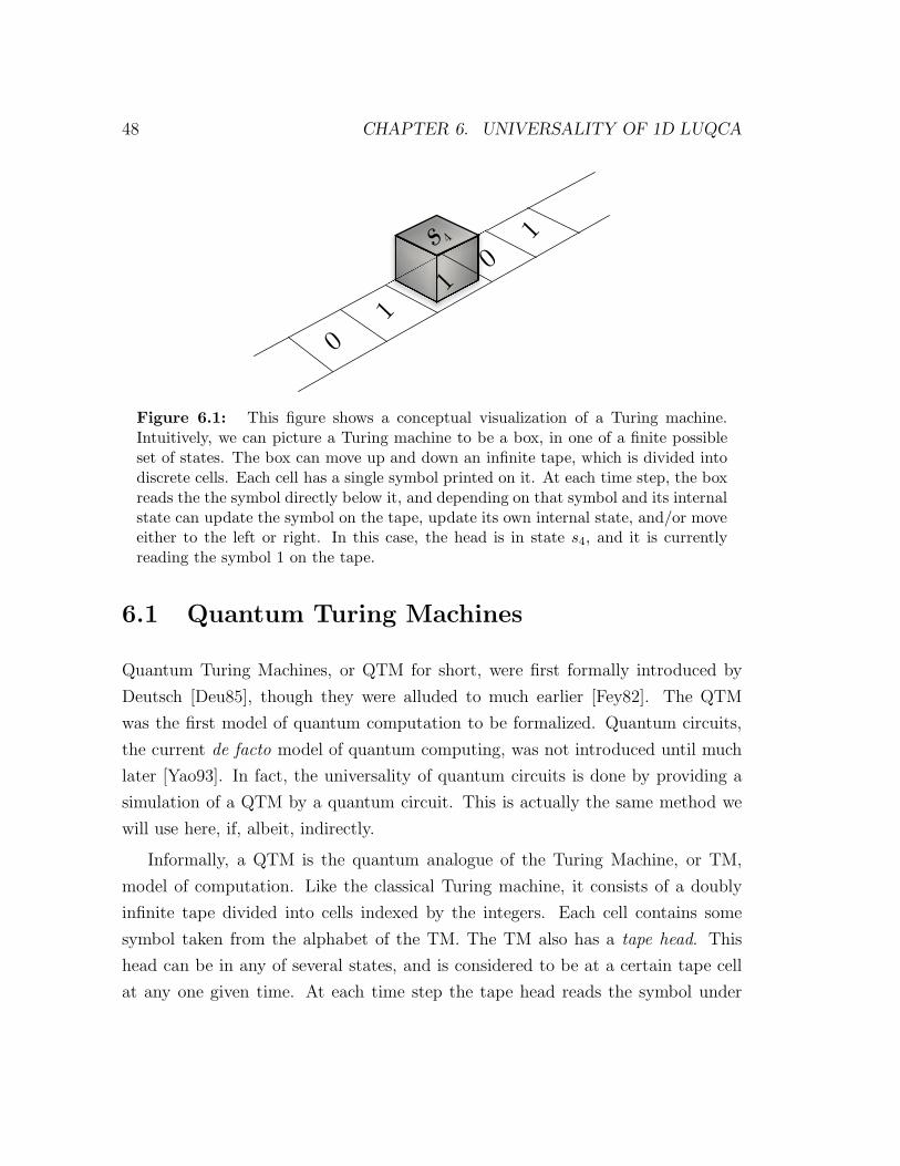
48 CHAPTER 6. UNIVERSALITY OF 1D LUQCA
0
s 4
1
1
1
0
Figure 6.1: This figure shows a conceptual visualization of a Turing machine.Intuitively, we can picture a Turing machine to be a box, in one of a finite possibleset of states. The box can move up and down an infinite tape, which is divided intodiscrete cells. Each cell has a single symbol printed on it. At each time step, the boxreads the the symbol directly below it, and depending on that symbol and its internalstate can update the symbol on the tape, update its own internal state, and/or moveeither to the left or right. In this case, the head is in state s4, and it is currentlyreading the symbol 1 on the tape.
6.1 Quantum Turing Machines
Quantum Turing Machines, or QTM for short, were first formally introduced by
Deutsch [Deu85], though they were alluded to much earlier [Fey82]. The QTM
was the first model of quantum computation to be formalized. Quantum circuits,
the current de facto model of quantum computing, was not introduced until much
later [Yao93]. In fact, the universality of quantum circuits is done by providing a
simulation of a QTM by a quantum circuit. This is actually the same method we
will use here, if, albeit, indirectly.
Informally, a QTM is the quantum analogue of the Turing Machine, or TM,
model of computation. Like the classical Turing machine, it consists of a doubly
infinite tape divided into cells indexed by the integers. Each cell contains some
symbol taken from the alphabet of the TM. The TM also has a tape head. This
head can be in any of several states, and is considered to be at a certain tape cell
at any one given time. At each time step the tape head reads the symbol under
6.1. QUANTUM TURING MACHINES 49
its current position, and depending on what symbol it reads and its current state,
it can decide to update the symbol currently being read on the tape, change its
current state, and/or move either to the left or to the right along the tape. See
Figure 6.1.
As opposed to classical deterministic Turing machines, where this decision is
made deterministically, or probabilistic Turing machines that can choose one of
many options probabilistically, the quantum Turing machine can choose to take
any subset of choices, all with predetermined amplitudes, in superposition.
The formalization of the QTM we will follow here is given by Bernstein and
Vazirani, in their seminal paper on quantum complexity theory [BV97,BV93].
Formally, a QTM M is defined as a triplet (Σ, S, δ), where Σ is a finite alphabet
with an identified blank symbol b, S is a finite set of states with an identified initial
state s0, and final state sf 6= s0 , and δ is a function
δ : S × Σ → CS×Σ×L,R,
which is referred to as the the quantum transition function. Here, C is defined to
be the set consisting of all c ∈ C such that there exists a deterministic algorithm
that computes the real and imaginary parts of c to within accuracy 2−n in time
polynomial in n.
The QTM has a two-way infinite tape of cells indexed by Z and a single
read/write tape head that moves along the tape.
A configuration, also known as an instantaneous description of the QTM, is a
description of the contents of the tape, the location of the tape head, and the state
s ∈ S of the finite control. At any time only a finite number of tape cells may
contain nonblank symbols.
Given a TM M , and a configuration c of M , the successor configuration c′ is
defined by applying the transition function to the current state s and currently
scanned symbol σ. We use cM→ c′ to denote that c′ follows from c in one step.
The convention is to require that the initial configuration of M satisfies the
following conditions:
50 CHAPTER 6. UNIVERSALITY OF 1D LUQCA
1. The tape head is in the cell indexed by the integer 0 (zero). This cell is called
the start cell.
2. The machine is in state s0.
We say that the QTM has input x ∈ (Σ − b)∗, if the symbol at position j
of the tape is xj for all 0 ≤ j ≤ |x| − 1, and equal to the blank tape symbol b
everywhere else.
Define HC to be the space of finite linear combinations of configurations of M .
Each element ψ ∈ HC is a possible superposition of M .
The QTM M defines a linear operator
UM : HC → HC ,
called the time evolution operator of M , in the following way: if M starts in
configuration c with current state p and scanned symbol σ, then after one step M
will be in the superposition of configurations
ψ =∑
j
αjcj,
where each nonzero αj corresponds to a transition δ(p, σ, τ, q, d), and cj is the new
configuration that results from applying this transition to c . Extending this map
to the entire space HS through linearity gives the linear time evolution operator
UM .
As with some previously defined QCA, a problem with the definition of the QTM
as described so far, is that there exist QTM with evolution that is not unitary, and
hence not physical. Again, following Bernstein and Vazirani [BV97] we will say
that M is well formed if its time evolution operator UM preserves Euclidean length.
In their paper, Bernstein and Vazirani show that being well formed is equivalent
to having unitary evolution in accordance with quantum mechanics.
Another important detail of quantum Turing machines refers to measurement.
6.2. PROOF OF UNIVERSALITY 51
Suppose that M ∈ QTM is in superposition
ψ =∑
j
αjcj.
If it is then measured configuration cj will be seen with probability |αj|2. Immedi-
ately after the measurement, the state of M will be cj with amplitude one.
6.2 Proof of Universality
We are now in a position to put together a proof of the universality of 1d-LUQCA.
We will start with the notion of universal quantum Turing machines.
Following [BV97], given quantum Turing machines M and M ′, suppose the
following holds: let D be the distribution obtained from repeatedly measuring
M on input x after T steps. Similarly, let D′ be the distribution obtained from
repeatedly measuring M ′ on input x after f(T ) steps for some function f . Then we
will say that M ′ simulates M with slowdown f and with accuracy ǫ if |D−D′| ≤ ǫ.
The following theorem from [BV97], which we state without proof, provides a
universal QTM:
Lemma 6.1 ( [BV97, Theorem 7.1]). There is a QTM Mu such that for any well-
formed QTM M , any ǫ > 0, and any T , Mu can simulate M with accuracy ǫ for T
steps with slowdown polynomial in T and 1ǫ.
We also need to introduce the notion of unidirectionality. A QTM M = (Σ, S, δ)
is said to be unidirectional if each state can be entered from at most one direction.
Formally, if 〈sj, σj , d1| δ |sk, σk〉 > 0 and 〈sj , σj, d2| δ |sk, σk〉 > 0 then d1 = d2.
We will need the following lemma from [BV97],
Lemma 6.2 ( [BV97, Lemma 5.5]). For every well-formed QTM M there is a
well-formed unidirectional QTM M ′ that simulates M , with constant slowdown.
Both of these results together imply that there is a QTM Mu that is both
universal, and unidirectional. We will need this fact later on.
52 CHAPTER 6. UNIVERSALITY OF 1D LUQCA
Lemma 6.3 ( [Wat95, Theorem 5.1]). Given any M ∈ QTM there exists a Q ∈ 1d-
PQCA which simulates M with constant slowdown.
Proof. Let M = (Γ, S, δ). Suppose, that M is unidirectional. If it is not, let M ′ be
a unidirectional QTM that simulates M . Let M ′ be the new M .
Now, let S = Sl ∪Sr where Sl (Sr) is the set off all states of M that are entered
only from the left (right).
Then, let Q = (Σ, f), where Σ = Σl × Σc × Σr such that,
Σl = Sl ∪ #Σc = Γ
Σr = Sr ∪ #
The quiescent state of Q is set to (#, b,#), where b is the blank tape cell of M .
Define f in the following way:
1. for each (sj , γj), (sk, γk) ∈ Sl × Γ let
〈sk, γk,#| f |sj , γj,#〉 = 〈sk, γk, L| δ |sj , γj〉
2. for each (sj , γj), (sk, γk) ∈ Sr × Γ let
〈#, γk, sk| f |#, γj, sj〉 = 〈sk, γk, R| δ |sj, γj〉
3. for each (sj , γj) ∈ Sl × Γ and (sk, γk) ∈ Sr × Γ let
〈#, sk, γk| f |sj, γj,#〉 = 〈sk, γk, R| δ |sj, γj〉〈sj, γj,#| f |#, sk, γk〉 = 〈sj , γj, L| δ |sk, γk〉
4. For all σj , σk ∈ Σ such that 〈σk| f |σj〉 is not defined by 1. - 3., let
〈σk| f |σj〉 =
1 if σj = σk,
0 otherwise.

6.2. PROOF OF UNIVERSALITY 53
If M is well-formed then f is a unitary operator. It is easy to verify from the
construction of f that Q does indeed simulate M .
Now, we can state the main result of this chapter.
Theorem V. There exists a 1d LUQCA which is universal for quantum computa-
tion.
Proof. From Lemma 6.1 we know that there exists a QTM Mu which is universal
for quantum computation. From Lemma 6.3 we know that there exists a 1d-PQCA
Qp which simulates Mu with at most constant slowdown. From Theorem III there
exists a 1d-LUQCA Ql that can simulate Qp with no slowdown. By construction,
Ql is a 1d-LUQCA that is universal for quantum computation.
Alternately, we can prove Theorem V in a more direct way. We take the same
construction as in Lemma 6.3 and apply the transformation described in the proof
of Theorem III. This would give us a construction of a universal QCA directly
within the LUQCA model.
This result concludes our discussion on the theory of QCA. In the following we
will shift our focus to the applications of this mathematical construction.

Part II
Applications
55

Chapter 7
Modelling Physical Systems
We stated before that one of our goals in developing a QCA formalism is to create a
powerful modelling tool for quantum systems. Classical CA are used for simulating
various phenomena based on classical information, such as sea ice formation, fluid
dynamics, or voter systems [TM87,CD98]. Similarly, we expect QCA to be able
to model different types of physical systems based on quantum information, with
dynamics which are based on time and space homogeneous local interactions.
Physical systems that fall in this category include Ising and Heisenberg interac-
tion Spin Chains, solid state NMR, and quantum lattice gases. We will be looking
at some of these systems in this section.
7.1 Spin Chains
Spin chains are perhaps the most obvious candidate for physical systems being
modelled with QCA. Indeed, Ising interaction spin chains, and in general, any spin
chain with a coupling Hamiltonian which commutes with its own lattice translations
can be implemented easily.
Suppose we have a linear spin chain of length N , indexed by n ∈ Z. Each spin n
is coupled to its nearest neighbour n+ 1, with a coupling Hamiltonian Jσ(n)z σ
(n+1)z ,
where J is the coupling strength constant. Note that the coupling Hamiltonian
does commute with its lattice translations. The Hamiltonian for the entire spin
57
58 CHAPTER 7. MODELLING PHYSICAL SYSTEMS
chain is:
HI =N−1∑
n=1
Jσ(n)z σ(n+1)
z .
It is a simple matter to give a discrete time approximation to such a spin chain.
First, we fix a time step interval ∆t. Our QCA model will allow for simulation of
the spin chain for time steps in multiples of ∆t. Hence, while the choice of ∆t is
arbitrary, it is important in determining the resolution of the simulation.
For a simulation of the Ising spin chain, the QCA lattice consists of a 1-
dimensional array, where each cell is a single qubit. The neighbourhood of each cell
n simply consists of the cell and its right neighbour n+ 1. The local rule operator
Un is given as:
Un = e−iJσ(n)z σ
(n+1)z ∆t.
The operator Vn is simply the identity operator. Note that the operator Un
commutes with its translations, that is, [Un, Um] = 0, for all n,m ∈ Z. Furthermore,
the global operator
U =
N−1∏
n=1
Un
satisfies
U = e−iHI∆t.
Hence, the QCA construction faithfully simulates the Ising spin chain on times
that are integer multiples of ∆t, as we desired.
A more complicated endeavor is to construct a QCA simulation of a spin chain
whose coupling Hamiltonians do not commute with each other. In particular we
examine the Heisenberg spin chain as an example. Let the coupling Hamiltonian
between spins n and n+ 1 be
H(n,n+1)H = J(σ(n)
x σ(n+1)x + σ(n)
y σ(n+1)y + σ(n)
z σ(n+1)z − 1l ⊗ 1l).
Here, note that H(n,n+1)H does not commute with all of its translations H(m,m+1)
H .
7.1. SPIN CHAINS 59
The Hamiltonian of the total system is
HH =N−1∑
n=1
H(n,n+1)H .
A QCA simulation of the Heisenberg spin chain presented above is still possible,
however, with the help of two powerful tools: Trotterization, and cell colouring.
The first technique is well known in physics, the second is a tool developed for
QCA. Together, they allow for simulation of complicated and almost arbitrary
Hamiltonians by QCA.
Trotterization is a technique by which a Hamiltonian is approximated using a
combination of non-commuting Hamiltonians whose sum adds up to the original
Hamiltonian. In other words, it is possible to approximate with bounded error the
evolution due to the Hamiltonian H = Ha +Hb by alternately evolving the system
under the Hamiltonians Ha and Hb even if these two do not commute. Precisely,
we can give a first-order approximation
e−i(Ha+Hb)∆t =(e−iHa∆t/ke−iHb∆t/k
)k+ δ.
In the case that ‖[Ha,Hb]‖∆t2 ≪ 1, the error δ is O(∆t2/k). Higher order
techniques can achieve error rates of O(∆tm + 1/km) at the cost of using O(2m)
gates. Though the number of gates increases exponentially, the time required for
each gate decreases exponentially as well.
In the case of our QCA simulation of the Heisenberg spin chain Hamiltonian
HH above, we have:
Ha =
⌈N−12 ⌉∑
n=1
H(2n−1,2n)H ,
and
Hb =
⌊N−12 ⌋∑
n=1
H(2n,2n+1)H .
Note that HH = Ha +Hb. The Hamiltonians Ha and Hb consist of the couplings
60 CHAPTER 7. MODELLING PHYSICAL SYSTEMS
from the even spins to their right neighbours and left neighbours respectively.
Our QCA evolution will consist of alternately evolving under Ha and Hb, using
a technique called cell colouring. Each cell will have two fields. The first field
is a state register, consisting of one qubit, which will hold the state of the spin
represented by the cell. The second field, called the active colour register, will also
consist of a single qubit. Initially, the colour register of each cell n is set to the
value n mod 2.
The QCA lattice used in this simulation is also one-dimensional, and the neigh-
bour set of each cell includes both the cell to the immediate right, and the immediate
left of the given cell. Let, U ′n be the Trotter step acting on the current cell state
register and the right neighbour state register. Using the first order approximation,
we have
U ′n = e−iH(n,n+1)∆t/k
for an appropriate value k. It is also possible to use higher order approximations.
The local update rule operator Un then consists of applying the operator U ′n if
and only if the current cell’s active colour register is set to one, and both left and
right neighbours have their colour registers set to zero. Operator Vn simply toggles
the active colour register.
It should be clear that this QCA construction simulates the Heisenberg spin
chain. Moreover, by using an appropriate operator U ′n, it is possible to simulate
any Hamiltonian with nearest neighbour couplings with this technique.
7.2 Quantum Lattice Gases
Quantum lattice gases have been studied for over a decade now [Bog98, BT98,
Mey96a,Yep98,LB05,LBM04]. In essence, they are the quantum analogue of clas-
sical lattice gases. The basic principles are the same in both the classical and
quantum cases: one starts with a discrete CA-based model that describes particles
on the lattice, and their movement. One can then take the continuous limit of
such CA and show that in this limit, the behavior of the CA mimics a well-known
differential equation.
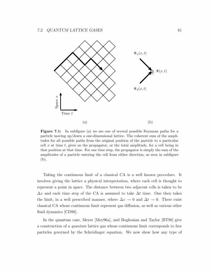
7.2. QUANTUM LATTICE GASES 61
Time t
Space x
(a) (b)
Figure 7.1: In subfigure (a) we see one of several possible Feynman paths for aparticle moving up/down a one-dimensional lattice. The coherent sum of the ampli-tudes for all possible paths from the original position of the particle to a particularcell x at time t, gives us the propagator, or the total amplitude, for a cell being inthat position at that time. For one time step, the propagator is simply the sum of theamplitudes of a particle entering the cell from either direction, as seen in subfigure(b).
Taking the continuous limit of a classical CA is a well known procedure. It
involves giving the lattice a physical interpretation, where each cell is thought to
represent a point in space. The distance between two adjacent cells is taken to be
∆x and each time step of the CA is assumed to take ∆t time. One then takes
the limit, in a well prescribed manner, where ∆x → 0 and ∆t → 0. There exist
classical CA whose continuous limit represent gas diffusion, as well as various other
fluid dynamics [CD98].
In the quantum case, Meyer [Mey96a], and Boghosian and Taylor [BT98] give
a construction of a quantum lattice gas whose continuous limit corresponds to free
particles governed by the Schrodinger equation. We now show how any type of
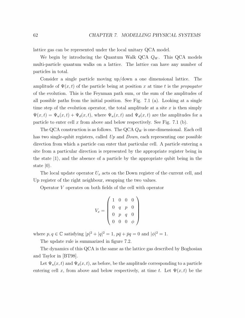
62 CHAPTER 7. MODELLING PHYSICAL SYSTEMS
lattice gas can be represented under the local unitary QCA model.
We begin by introducing the Quantum Walk QCA QW . This QCA models
multi-particle quantum walks on a lattice. The lattice can have any number of
particles in total.
Consider a single particle moving up/down a one dimensional lattice. The
amplitude of Ψ(x, t) of the particle being at position x at time t is the propagator
of the evolution. This is the Feynman path sum, or the sum of the amplitudes of
all possible paths from the initial position. See Fig. 7.1 (a). Looking at a single
time step of the evolution operator, the total amplitude at a site x is then simply
Ψ(x, t) = Ψu(x, t) + Ψd(x, t), where Ψu(x, t) and Ψd(x, t) are the amplitudes for a
particle to enter cell x from above and below respectively. See Fig. 7.1 (b).
The QCA construction is as follows. The QCAQW is one-dimensional. Each cell
has two single-qubit registers, called Up and Down, each representing one possible
direction from which a particle can enter that particular cell. A particle entering a
site from a particular direction is represented by the appropriate register being in
the state |1〉, and the absence of a particle by the appropriate qubit being in the
state |0〉.The local update operator Ux acts on the Down register of the current cell, and
Up register of the right neighbour, swapping the two values.
Operator V operates on both fields of the cell with operator
Vx =
1 0 0 0
0 q p 0
0 p q 0
0 0 0 φ
where p, q ∈ C satisfying |p|2 + |q|2 = 1, pq + pq = 0 and |φ|2 = 1.
The update rule is summarized in figure 7.2.
The dynamics of this QCA is the same as the lattice gas described by Boghosian
and Taylor in [BT98].
Let Ψu(x, t) and Ψd(x, t), as before, be the amplitude corresponding to a particle
entering cell x, from above and below respectively, at time t. Let Ψ(x, t) be the
7.2. QUANTUM LATTICE GASES 63
V U
x x+1 x+2 x+3 x+4x-1x-2x-3
Up Register Down Register
Figure 7.2: This figure gives a visual representation of the quantum walk QCA.The cells are arranged from left to right, with the two registers of each cell—Up andDown—stacked vertically. The update rule for a single cell—the one with a blackborder—can be seen. It consists of the operator U acting on it and the only cell inits neighbourhood: the one directly to the right, shown with a grey outline. Theoperator V acts on both registers of the cell.
total amplitude corresponding to the presence of a particle in cell x at time t, that
is Ψ(x, t) = Ψu(x, t) + Ψd(x, t).
Then, we have that
Ψu(x, t+ ∆t) = qΨu(x− ∆x, t) + pΨd(x+ ∆x, t)
Ψd(x, t+ ∆t) = qΨd(x+ ∆x, t) + pΨu(x− ∆x, t)
We can proceed according to Boghosian and Taylor [BT98], and take the con-
tinuous limit of our QCA ∆x2 → 0 and ∆t → 0, using the Chapman-Enskog
method [CD98]. Doing so reveals that Ψ(x, t) obeys the equation:
∂
∂tΨ(x, t) =
i
2m
∂2
∂x2Ψ(x, t),
which is the equation for a freely moving particle of massm = ip/q in one dimension.
Using the same construction techniques, we can also describe a freely moving
particle in two or three dimensions. We can construct QCA that simulate other
quantum lattice gases like the ones proposed in [Mey96a]. Most, if not all, quantum
lattice gases, whether single or multi-particle, can be described as local unitary
QCA.
We now finish our discussion on the expressive powers of the QCA model here
64 CHAPTER 7. MODELLING PHYSICAL SYSTEMS
presented. In the next chapter we continue with a discussion of how to take these
mathematical models and implement them in quantum hardware.
Chapter 8
Quantum Computation
In previous chapters, we discussed how our unitary QCA can be used to model
physical systems. We also studied how universal quantum computation can be
accomplished using only QCA primitives.
In this chapter we will look into bridging the gap by using QCA as a theoretical
framework for implementing quantum computation.
A clear advantage of working in the QCA model over quantum circuits, in re-
gards to physical implementations of quantum computation, is that QCA have con-
siderably fewer restrictions on the underlying hardware. In particular, as opposed
to direct implementations of quantum circuits, the QCA model does not assume
independent control over qudits. Rather, all qudits are to be addressed collectively
in parallel. While a priori the latter requirement might not be any easier than the
former, in some experimental setups, we argue below, global control is simpler to
implement than individual addressability.
The QCA model also more closely resembles what is currently achievable in
several current quantum computer implementations. For example, if qudits are
represented by physical spins, and the control of such spins is achieved through the
use of magnetic pulses, as is the case in NMR or ESR, then it may be more reason-
able to consider all spins as being subjected to the same pulse sequences, rather than
having the ability to address spins individually. This is because in these schemes,
the spins are addressed via magnetic pulses that target their particular resonant
65
66 CHAPTER 8. QUANTUM COMPUTATION
frequencies. In a highly regular molecule like a nanotube, all spins are of the same
species—carbons in this instance—and they all have similar chemical shifts. Hence,
distinguishing them is not possible. In order to have individual addressability usu-
ally requires a highly asymmetric molecule, with possibly many different species of
atoms. Other techniques for differentiation might include gradient fields. In short,
global control generally is a less difficult constraint than individual control over
qubits is.
The same can be said about many other physical quantum computer proposals.
In this section we will concentrate on implementing QCA on NMR, since most of
the groundwork for this implementation has already been laid out.
8.1 Coloured QCA
In Chapter 7, we considered cell colouring as a useful QCA programming technique.
As with other computation models, where a programming technique can formalized
into its own subset model, and then shown to be equivalent to the general model
(such as multi-track Turing machines), we can do the same with coloured QCA.
First, we will define the notion of a totalistic transition function for QCA. It
is the quantum analog of totalistic CA, in which the transition function depends
only on the total number of neighbouring cells in each of the possible cell states.
Essentially, a transition update function is totalistic when it affects only the value of
the target cell in a manner which depends only on how many of the cell’s neighbours
are in particular states, rather than on which state any particular neighbour is in.
Definition 8.1. Given a QCA Q = (L,Σ,N , U0, V0), we call the update function
U0 : (HΣ)⊗N → (HΣ)⊗N totalistic if it can be expressed as a collection of single-cell
operations on cell 0 controlled by the computational basis states of the neighbour-
hood N \0, and U0 commutes with every operator SWAP x,y, which simply swaps
the contents of cells x and y, where x, y ∈ N \ 0. If Q has a totalistic update
function, then we call Q a totalistic QCA.
Next, we wish to formalize the notion of a coloured QCA. For this model, we
will fix the neighbourhood scheme to include only directly adjacent cells. That is,
8.1. COLOURED QCA 67
N = x ∈ Zd : ‖x‖1 ≤ 1. However, first we will define the set of permissible
colourings of a lattice.
Definition 8.2. Given a lattice L = Zd and a neighbourhood scheme N , we define
a correct k-colouring for a lattice as a periodic mapping C : L→ 0, 1, . . . , k − 1,such that no two neighbouring cells in L are assigned the same colour.
We may think of cell colour as an inherent property of each cell. However, it
may also be helpful to consider cell colour as classical information which is being
stored with each cell in such a way that the local transition function does not alter
this information. We can now finally give a definition for the coloured QCA. Recall
that the neighbourhood scheme N is fixed.
Definition 8.3 (CQCA). A Colored QCA or CQCA is a 5-tuple (L,C,Σ,U , c)consisting of a lattice L = Z
d, a correct k-colouring C, a finite set Σ of cell states,
a sequence of T totalistic unitary operators U =(U
(0)0 , U
(1)0 , . . . , U
(T−1)0
), with
U(j)0 : (HΣ)⊗N → (HΣ)⊗N , and a sequence of T colours c = (c0, c1, . . . , c(T−1)),
labeled by integers 0 ≤ cj < k.
The local transition operation consists of applying U(j)x to each cell x with colour
C(x) = cj at time step t = j + nT , where 0 ≤ j < T and n ∈ Z.
Note that since C is a correct k-colouring, any two operators U(j)x acting non-
trivially on two cells of the same colour at the same time will commute.
CQCA can be simply considered as a shorthand for the cell colouring technique
we introduced in Chapter 7. As such, it should be clear that CQCA are a subset
of unitary QCA.
Theorem VI. For every CQCA Q there is a QCA Q′ that simulates the same
evolution exactly.
Proof. We may incorporate the colour information of each cell of the CQCA Q
within an additional colour register for each cell of the QCA Q′. Now, it suffices
to add one extra clock register to each cell, initialized to 0. The update operator
Ux simply applies U(j)x conditional on both C(x) and the clock register of cell x
68 CHAPTER 8. QUANTUM COMPUTATION
being set to j. In order to ensure that Ux commutes with its translations, we must
ensure that the colours of all the neighbours of x are consistent with the colouring C
before applying the appropriate operator. Otherwise, Ux should act as the identity
operator. The read operator Vx simply increments the clock register, modulo T .
What is more surprising is the converse result; that all unitary QCA can be
rephrased in the CQCA formalism.
Theorem VII. For every QCA Q there is a CQCA Q′ that simulates the same
evolution exactly.
Proof. Given the QCA Q = (L,Σ,N , U0, V0), we will use the same lattice L and
alphabet Σ. The neighbourhood scheme for the CQCA, N ′ is fixed by definition.
We also need to provide a correct k-colouring of the lattice. To this end, it suffices
to provide a colouring C with the property that that no neighbourhood Nx of Q or
N ′x of Q′ contains two cells with the same colour. Now, we need to construct a se-
quence U of update operators. Note that conditional on a cell x having a particular
colour, single-qudit operations on x, and the controlled-NOT operation targetting
x are colour-totalistic operations. Because we insisted on a colouring such that
no neighbourhood N ′x contains two cells of the same colour, such controlled-NOT
operations can always be controlled by a single neighbouring qubit. Now, given
an implementation of the unitary update operation U0 of Q using single-qudit and
nearest-neighbour controlled-NOT operations, we can give a sequence of colour-
totalistic operations which perform U0 on a neighbourhood Nx of a cell x of a
specific colour. By performing a similar sequence of operations for each colour in
our colouring C, we effectively perform Ux for each cell x. Since each update oper-
ation Ux commutes with the other update operations, we have effectively simulated
the update transition operation of Q. Finally, we can perform the single-qudit
operations Vx for each cell colour.
This last result is of major importance as it allows us to implement any uni-
tary QCA algorithm on a pulse-driven quantum computer, as proposed by Seth
Lloyd [Llo93], and further developed by Simon Benjamin [Ben00,BB03] and oth-
ers [BW03]. The scheme involves using large molecules comprised of two or more
8.1. COLOURED QCA 69
different species of spin- 12
particles, arranged in repetitive structures, such as crys-
tals or polymers, to store the quantum data. It then evolves the system using series
of magnetic pulses that address of all spins of any one particular species.
In order to implement a given QCA in the pulse-driven computation model, we
first convert the QCA into one which uses a two-state alphabet. This can be done
by expanding each cell into ⌈log |Σ|⌉ cells to encode the states of Σ with a binary
alphabet, then adjusting the neighbourhood scheme N accordingly. We then apply
the construction in Theorem VII. With this, and the techniques of Lloyd et. al., it
would be possible to implement any QCA algorithm using NMR and an appropriate
molecule.
We choose NMR and pulse driven quantum computing devices to show a phys-
ical implementation of local unitary QCA. However, this should not be taken to
be the only possible implementation of QCA. There are many other physical sys-
tems, like optical lattices [BLR04], cavity QED, among others [Kan98, KBST06],
that seem better suited to implementing QCA, rather than the more traditional
quantum circuits.

Chapter 9
Single Spin Measurement
In this chapter we will present a very interesting application of the QCA framework
we have developed so far. This application of QCA is interesting for several rea-
sons. First and foremost, it tackles a problem of significant importance in Physics,
specifically, in metrology. The solution developed here is the most efficient method
put forth so far. Also, the solution showcases several QCA techniques, and how
QCA can be applied to real-world Physics.
We will begin this chapter by introducing the problem we wish to solve, in
its full context. Next we will develop the algorithm, in a completely theoretical
fashion, i.e. completely in the abstract without referring to any actual physical
system, using our QCA framework. We will then analyse the algorithm in this
abstract framework: we will find runtimes, error robustness, and scaling. Finally,
after the algorithm has been fully developed in the abstract, we will show how to
implement it using a real world physical system, and its Hamiltonians.
The layout of this chapter also showcases the power of our QCA framework.
Thanks to it, we are able to abstract away the details of the actual physical system.
We can then develop and study our algorithm in the abstract without being bogged
down by implementation details. We only re-introduce these physical details at
the end, when we wish to actually take the fully developed algorithm study its
implementation in a laboratory setting.
We now begin by introducing the problem we wish to solve. We will assume
71
72 CHAPTER 9. SINGLE SPIN MEASUREMENT
basic knowledge of NMR QIP.
9.1 Problem Description
We present the description of the problem in simple abstract terms. Suppose we
want to amplify the signal from a single spin-12
particle. That is, we have a single
spin-12
particle, and we want to create a large ensemble of spins whose bulk angular
momentum resembles the original spin in a particular basis. Note that this is not
cloning, since a basis needs to be set beforehand. Succinctly, we want a unitary
procedure U that maps the state
(α|0〉 + β|1〉)︸ ︷︷ ︸Amplified Spin
⊗ |0〉⊗N
︸ ︷︷ ︸Ancillae
to the state
α|0〉⊗(N+1) + β|1〉⊗(N+1),
where |0〉 and |1〉 form the basis in which we wish to amplify. The main application
of such algorithm is to perform a measurement in situations where bulk magneti-
zation is needed in order to achieve a detectable signal, such as with NMR. Hence,
the algorithm needs to be extremely efficient: the whole procedure needs to be
completed before decoherence can destroy the desired value. The value N will also
tend to be reasonably large, in the order of 107 or 108, in order to get a reasonable
signal in NMR.
Figure 9.1 shows a simple quantum circuit solution.
However, this circuit approach does have several shortcomings. First and fore-
most, it requires individually addressing N different spins. For large N , in most
laboratory conditions, this is not feasible. Supposing that one could get around this
first hurdle, one would still need to perform N individual gates before decoherence
destroys the data. Again, this is not likely to be feasible in most experimental
settings.
A plausible experimental setup is the following. We use a crystal as a probe,
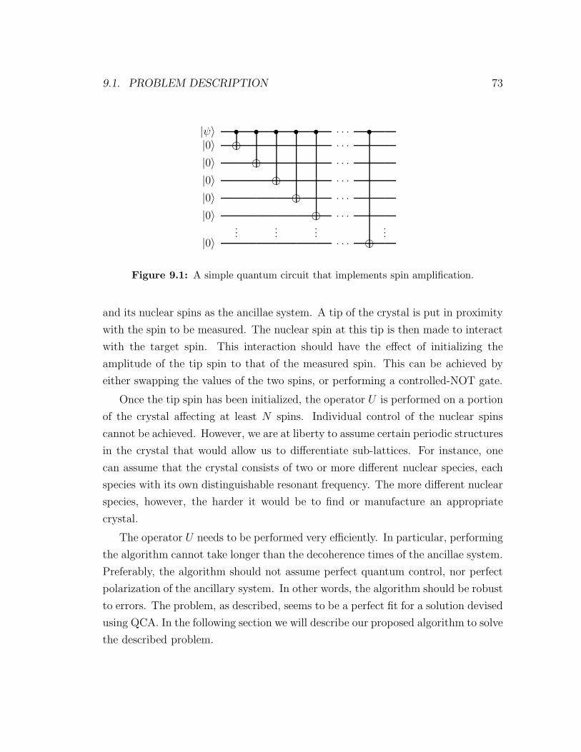
9.1. PROBLEM DESCRIPTION 73
|ψ〉 • • • • • . . . •|0〉 . . .
|0〉 . . .
|0〉 . . .
|0〉 . . .
|0〉 . . ....
......
...|0〉 . . .
Figure 9.1: A simple quantum circuit that implements spin amplification.
and its nuclear spins as the ancillae system. A tip of the crystal is put in proximity
with the spin to be measured. The nuclear spin at this tip is then made to interact
with the target spin. This interaction should have the effect of initializing the
amplitude of the tip spin to that of the measured spin. This can be achieved by
either swapping the values of the two spins, or performing a controlled-NOT gate.
Once the tip spin has been initialized, the operator U is performed on a portion
of the crystal affecting at least N spins. Individual control of the nuclear spins
cannot be achieved. However, we are at liberty to assume certain periodic structures
in the crystal that would allow us to differentiate sub-lattices. For instance, one
can assume that the crystal consists of two or more different nuclear species, each
species with its own distinguishable resonant frequency. The more different nuclear
species, however, the harder it would be to find or manufacture an appropriate
crystal.
The operator U needs to be performed very efficiently. In particular, performing
the algorithm cannot take longer than the decoherence times of the ancillae system.
Preferably, the algorithm should not assume perfect quantum control, nor perfect
polarization of the ancillary system. In other words, the algorithm should be robust
to errors. The problem, as described, seems to be a perfect fit for a solution devised
using QCA. In the following section we will describe our proposed algorithm to solve
the described problem.
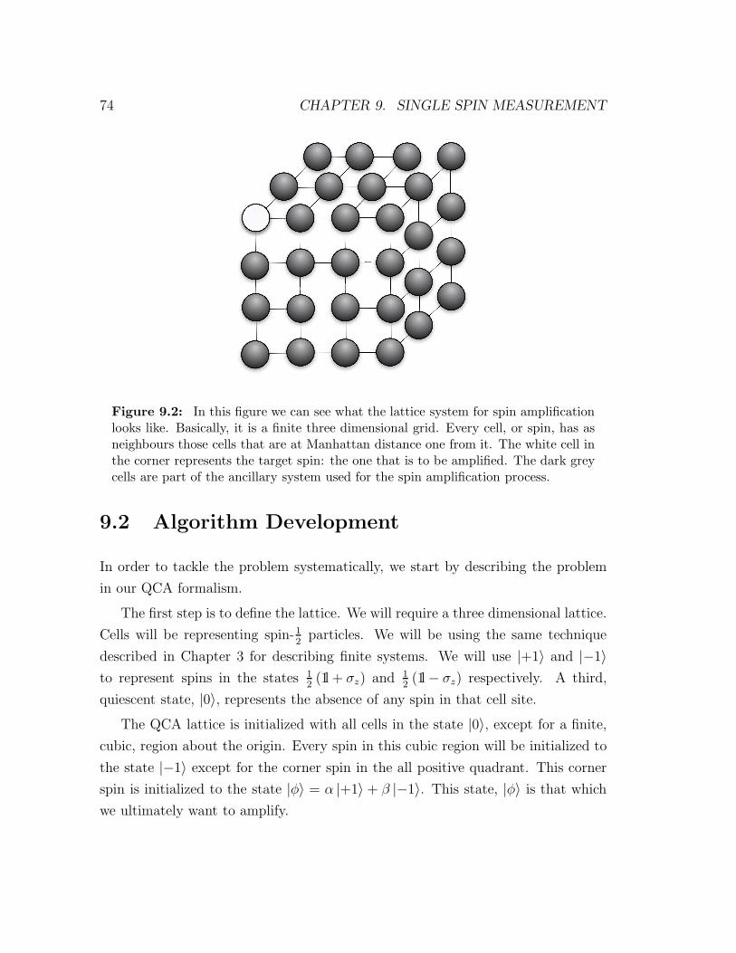
74 CHAPTER 9. SINGLE SPIN MEASUREMENT
Figure 9.2: In this figure we can see what the lattice system for spin amplificationlooks like. Basically, it is a finite three dimensional grid. Every cell, or spin, has asneighbours those cells that are at Manhattan distance one from it. The white cell inthe corner represents the target spin: the one that is to be amplified. The dark greycells are part of the ancillary system used for the spin amplification process.
9.2 Algorithm Development
In order to tackle the problem systematically, we start by describing the problem
in our QCA formalism.
The first step is to define the lattice. We will require a three dimensional lattice.
Cells will be representing spin-12
particles. We will be using the same technique
described in Chapter 3 for describing finite systems. We will use |+1〉 and |−1〉to represent spins in the states 1
2(1l + σz) and 1
2(1l − σz) respectively. A third,
quiescent state, |0〉, represents the absence of any spin in that cell site.
The QCA lattice is initialized with all cells in the state |0〉, except for a finite,
cubic, region about the origin. Every spin in this cubic region will be initialized to
the state |−1〉 except for the corner spin in the all positive quadrant. This corner
spin is initialized to the state |φ〉 = α |+1〉 + β |−1〉. This state, |φ〉 is that which
we ultimately want to amplify.
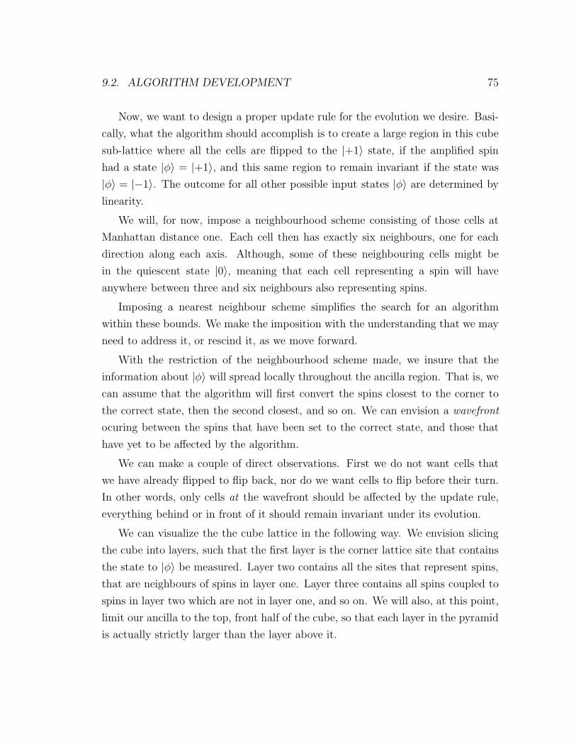
9.2. ALGORITHM DEVELOPMENT 75
Now, we want to design a proper update rule for the evolution we desire. Basi-
cally, what the algorithm should accomplish is to create a large region in this cube
sub-lattice where all the cells are flipped to the |+1〉 state, if the amplified spin
had a state |φ〉 = |+1〉, and this same region to remain invariant if the state was
|φ〉 = |−1〉. The outcome for all other possible input states |φ〉 are determined by
linearity.
We will, for now, impose a neighbourhood scheme consisting of those cells at
Manhattan distance one. Each cell then has exactly six neighbours, one for each
direction along each axis. Although, some of these neighbouring cells might be
in the quiescent state |0〉, meaning that each cell representing a spin will have
anywhere between three and six neighbours also representing spins.
Imposing a nearest neighbour scheme simplifies the search for an algorithm
within these bounds. We make the imposition with the understanding that we may
need to address it, or rescind it, as we move forward.
With the restriction of the neighbourhood scheme made, we insure that the
information about |φ〉 will spread locally throughout the ancilla region. That is, we
can assume that the algorithm will first convert the spins closest to the corner to
the correct state, then the second closest, and so on. We can envision a wavefront
ocuring between the spins that have been set to the correct state, and those that
have yet to be affected by the algorithm.
We can make a couple of direct observations. First we do not want cells that
we have already flipped to flip back, nor do we want cells to flip before their turn.
In other words, only cells at the wavefront should be affected by the update rule,
everything behind or in front of it should remain invariant under its evolution.
We can visualize the the cube lattice in the following way. We envision slicing
the cube into layers, such that the first layer is the corner lattice site that contains
the state to |φ〉 be measured. Layer two contains all the sites that represent spins,
that are neighbours of spins in layer one. Layer three contains all spins coupled to
spins in layer two which are not in layer one, and so on. We will also, at this point,
limit our ancilla to the top, front half of the cube, so that each layer in the pyramid
is actually strictly larger than the layer above it.
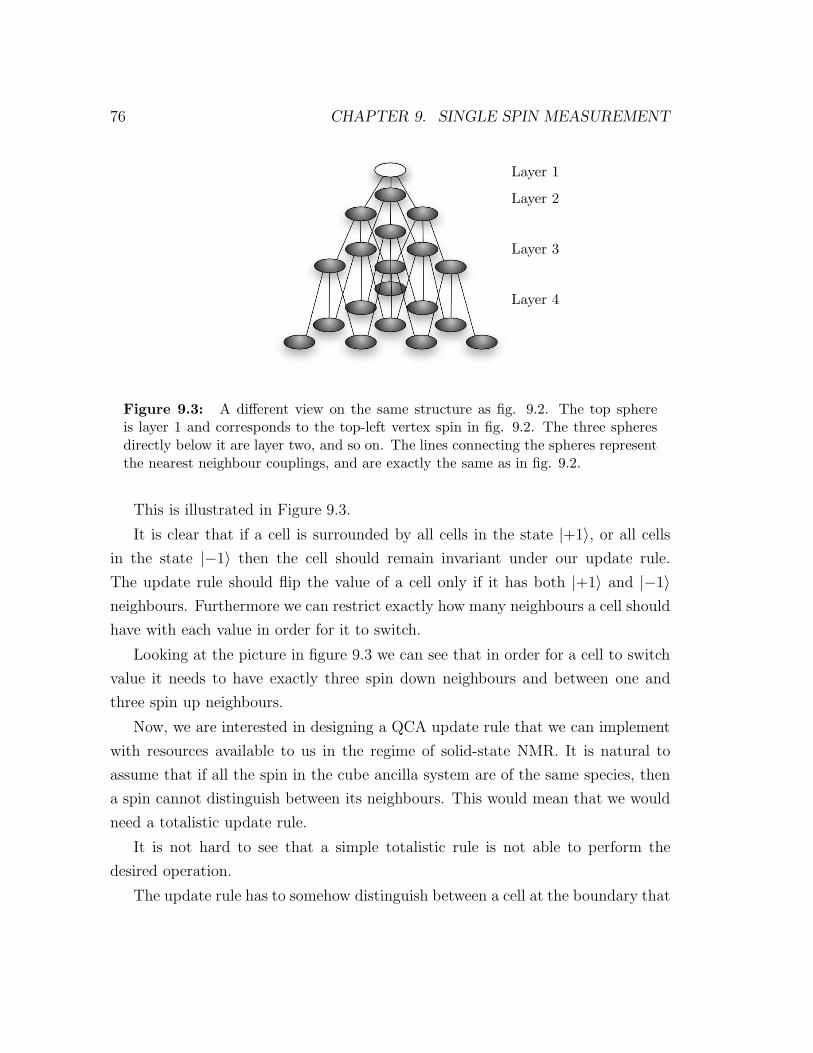
76 CHAPTER 9. SINGLE SPIN MEASUREMENT
Layer 1
Layer 2
Layer 3
Layer 4
Figure 9.3: A different view on the same structure as fig. 9.2. The top sphereis layer 1 and corresponds to the top-left vertex spin in fig. 9.2. The three spheresdirectly below it are layer two, and so on. The lines connecting the spheres representthe nearest neighbour couplings, and are exactly the same as in fig. 9.2.
This is illustrated in Figure 9.3.
It is clear that if a cell is surrounded by all cells in the state |+1〉, or all cells
in the state |−1〉 then the cell should remain invariant under our update rule.
The update rule should flip the value of a cell only if it has both |+1〉 and |−1〉neighbours. Furthermore we can restrict exactly how many neighbours a cell should
have with each value in order for it to switch.
Looking at the picture in figure 9.3 we can see that in order for a cell to switch
value it needs to have exactly three spin down neighbours and between one and
three spin up neighbours.
Now, we are interested in designing a QCA update rule that we can implement
with resources available to us in the regime of solid-state NMR. It is natural to
assume that if all the spin in the cube ancilla system are of the same species, then
a spin cannot distinguish between its neighbours. This would mean that we would
need a totalistic update rule.
It is not hard to see that a simple totalistic rule is not able to perform the
desired operation.
The update rule has to somehow distinguish between a cell at the boundary that
9.2. ALGORITHM DEVELOPMENT 77
Figure 9.4: A crystal with two types of nuclei A and B, one represented as light grayspheres, the other dark grey. Each species A is neighboured by only B type nucleiand vice-versa. The lines connecting the spheres represent the nearest neighbourcouplings. The white sphere represents the spin we wish to measure. This spin iscoupled to the dark grey nucleus in the top-left vertex.
requires to be flipped on this iteration, and one that was flipped on the last iteration
and hence needs to stay unchanged. Unfortunately, given only the information that
we are currently holding in our lattice, both types of cell are indistinguishable.
Fortunately, as described in Section 9.1, we are at liberty to use a crystal struc-
ture with more species of spin. We can therefore use a Coloured QCA, as defined
in Chapter 8. The update rule would then be colour totalistic.
We only need two colours to achieve our purpose. We redefine our lattice to
split lattice sites into two colours, say black and white. Each black cell is connected
to white cells only and vice versa. See figure 9.4 for details.
As before, in order to more easily illustrate our algorithm it is best to visualize
the cube lattice as a pyramid, as illustrated in fig. 9.5.
Each layer includes spins of only one species, layer one being all A, layer two all
B, layer three all A again and so on. We envision taking only half the cube lattice,
so that each layer is larger than the previous one. Layer i has i more spins than
layer i− 1.
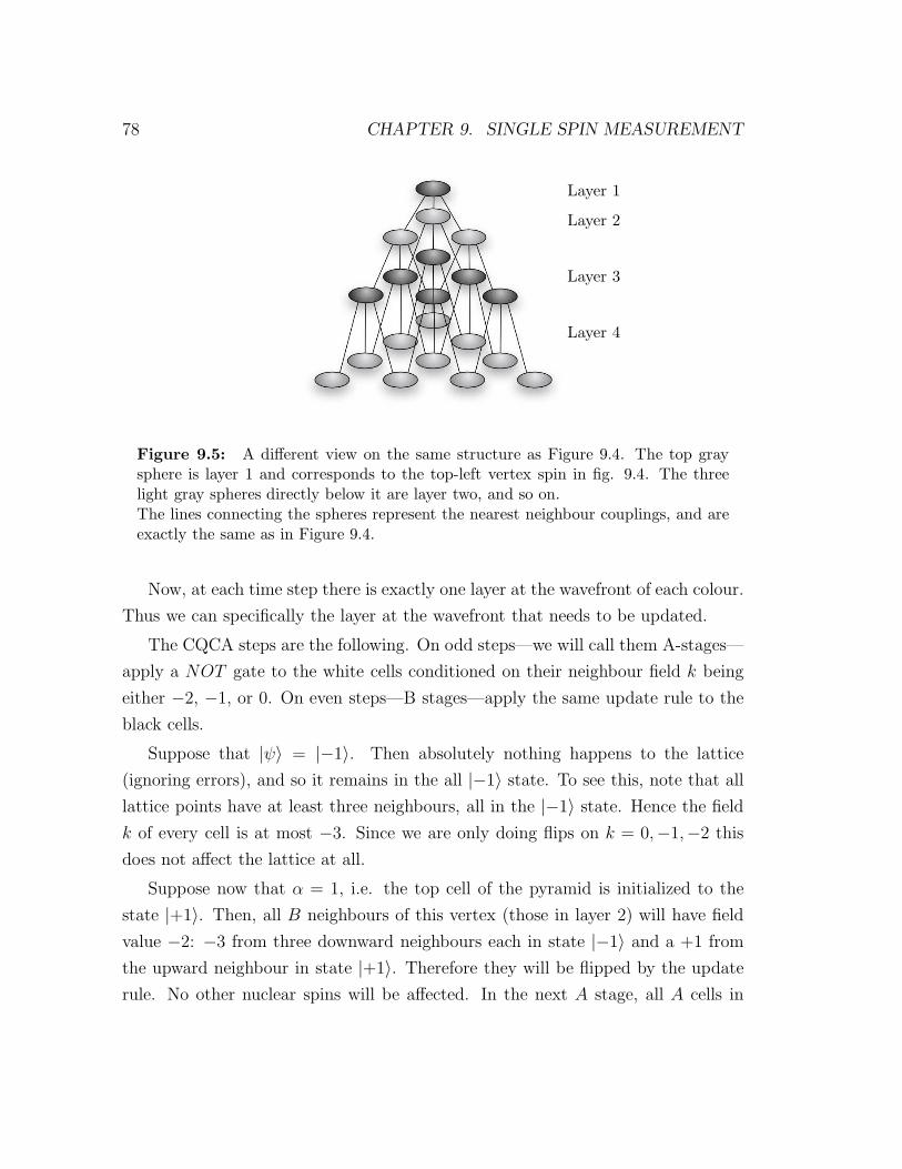
78 CHAPTER 9. SINGLE SPIN MEASUREMENT
Layer 1
Layer 2
Layer 3
Layer 4
Figure 9.5: A different view on the same structure as Figure 9.4. The top graysphere is layer 1 and corresponds to the top-left vertex spin in fig. 9.4. The threelight gray spheres directly below it are layer two, and so on.The lines connecting the spheres represent the nearest neighbour couplings, and areexactly the same as in Figure 9.4.
Now, at each time step there is exactly one layer at the wavefront of each colour.
Thus we can specifically the layer at the wavefront that needs to be updated.
The CQCA steps are the following. On odd steps—we will call them A-stages—
apply a NOT gate to the white cells conditioned on their neighbour field k being
either −2, −1, or 0. On even steps—B stages—apply the same update rule to the
black cells.
Suppose that |ψ〉 = |−1〉. Then absolutely nothing happens to the lattice
(ignoring errors), and so it remains in the all |−1〉 state. To see this, note that all
lattice points have at least three neighbours, all in the |−1〉 state. Hence the field
k of every cell is at most −3. Since we are only doing flips on k = 0,−1,−2 this
does not affect the lattice at all.
Suppose now that α = 1, i.e. the top cell of the pyramid is initialized to the
state |+1〉. Then, all B neighbours of this vertex (those in layer 2) will have field
value −2: −3 from three downward neighbours each in state |−1〉 and a +1 from
the upward neighbour in state |+1〉. Therefore they will be flipped by the update
rule. No other nuclear spins will be affected. In the next A stage, all A cells in
9.3. ALGORITHM ANALYSIS 79
layer 3 will be flipped, and so on. In n stages all cells in the first n layers will be
flipped to |+1〉.After n stages there will be N = 1
6(n + 1)n(n − 1) nuclear spins pointing up.
This shows that only O( 3√N) stages are required to obtain a total of N cells in
the proper state. In a physical implementation scenario one would then be able to
perform a measurement. Before getting into the physical details, we can further
analyse the algorithm in the abstract, and test its performance.
9.3 Algorithm Analysis
In the last section we developed and presented an algorithm that seems to solve
the problem we set up to do at the beginning of this chapter. However, we do not
know yet if it trully complies with all the criteria we established.
Let us start by discussing run times vs. decoherence times. Ultimately, this
question cannot be answered fully until an actual physical implementation and its
details are discussed. However, we can easily see that we are in a very good position,
time-complexity-wise. The algorithm runs in O( 3√N), as discussed before. If we
assume that any algorithm can do only nearest neighbour interactions, and that
any lattice used is at most three-dimensional, then our algorithm is optimal in run
time.
In other words, regardless of implementation details, no other algorithm can
hope to perform better asymptotically. This seems to put us in a very good position
indeed.
We are even in a better position. Another observation we can make without
knowing the physical implementation details is that the update rules are ‘phase
oblivious’. What we mean by this is that in between each update rule we can
subject all our cells to any sort of dephasing channel, and this would not affect
the ultimate outcome. In a sense, our CQCA is a classical CA built to run on a
quantum a system.
We do not know, at this stage, how the update rule itself is implemented. It may
very well be that major phase errors during the application of the rule itself, may
80 CHAPTER 9. SINGLE SPIN MEASUREMENT
cause the update to fail. However, we need only concern ourselves that the phase
error rate is low enough at the time-scale of a single update rule implementation,
and not at the time-scale of the whole algorithm completion.
Recall that there are two important parameters when discussing decoherence in
this scenario: t1 and t2 times. The latter describes how long it takes the system
to lose its phase information, the former its amplitude information. It is the case
that t2 times always considerably much shorter than t1. Fortunately, the t2 of the
ancillae system used, as expressed above, need only be longer than the time required
to implement the pulse sequence for a single update phase. Since the update phase
consists of a constant, and likely small, number of magnetic pulses it is reasonable
to assume that it can be achieved in under the t2 times. Regardless, this is an
implementation detail and lies outside the purview of this section.
We can now safely ignore phase errors for the rest of this section, since we have
now shown that they only concern the implementer of the actual update rule. What
we may not ignore is bit flip errors.
A single bit-flip error in the cube lattice by itself does not drastically change
the overall field, however, if this bit flips during the running of the algorithm it has
the potential to influence all lattice points in a radius around it, by changing their
neighbour fields during the pulse sequence.
The first fact to notice is that errors inside the pyramid are less critical than
errors on the faces, or worse, edges, of the pyramid. The reason for this is that inside
the pyramid all lattice points have exactly 6 neighbours. If one flips erroneously its
neighbours still have 5 neighbours each in the correct state.
Take an interior lattice point that is in the state |−1〉 and should be flipped to
|+1〉 in the next pulse sequence. Since it is supposed to flip it should have three
positive neighbours and three negative ones. Suppose that an upward neighbour
has an error, then it will have two positive and four negative. This is, however, not
a problem. The lattice point in question will have a field value k = −2, instead of
k = 0, but will still be flipped correctly.
Contrast this to the case where a bit flip occurs along the edge of the pyramid.
In this case the field of the lower neighbours to a lattice point with error will go
9.3. ALGORITHM ANALYSIS 81
from having a field of −2 to a field of −4 and will no longer be correctly flipped at
all. The error will then propagate downwards.
We need to better understand how our algorithm copes with errors in general.
We want to know how large the bit flip error rate can be, and have our algorithm
still achieve its goal. We would like to know how the error scales with lattice size,
and how the field scales with the error rate.
Now, unfortunately, in order to fully understand our algorithm behaviour under
all sorts of different conditions we would need a working a quantum computer, to
do a fully coherent, quantum mechanical, simulation of the system under different
error conditions.
Since we cannot do that, we proceed by creating a model of a model, essentially.
We start by recalling that we built our algorithm ‘phase oblivious.’ Hence, we con-
veniently ignore the phase of qubit in the cell lattice. Without phase information,
we can view each cell as having a probability of being in either state |+1〉 or |−1〉.Instead of probabilities, we can instead use actual values, chosen at random with
the right probabilities, and average over many samples. Essentially, we are creating
a Monte Carlo model of our CQCA model in order to be able to simulate on current
computer hardware and obtain meaningful results.
Our purpose in numerically simulating the system is to inform future engineering
studies of single spin detection. At this time we will explore the scalability and
error propagation. There remain serious technical challenges before any realistic
experimental study can be attempted.
Essentially, we are interested in knowing how well the algorithm performs under
various error models.
There are essentially two sources of error. There are the errors in pre-existing
in the lattice, due to imperfect polarization of the crystal used as our ancillary
measurement system. We will call ǫ0 the deficiency in polarization. For instance,
in a crystal with 90% polarization, we will have ǫ0 = 0.1. Small lattice defects,
like impurities, are also modelled in this way, since they represent errors that are
there to begin with, rather than being introduced by the faulty application of the
algorithm itself. Larger lattice defects, like dislocations, were not modelled. These
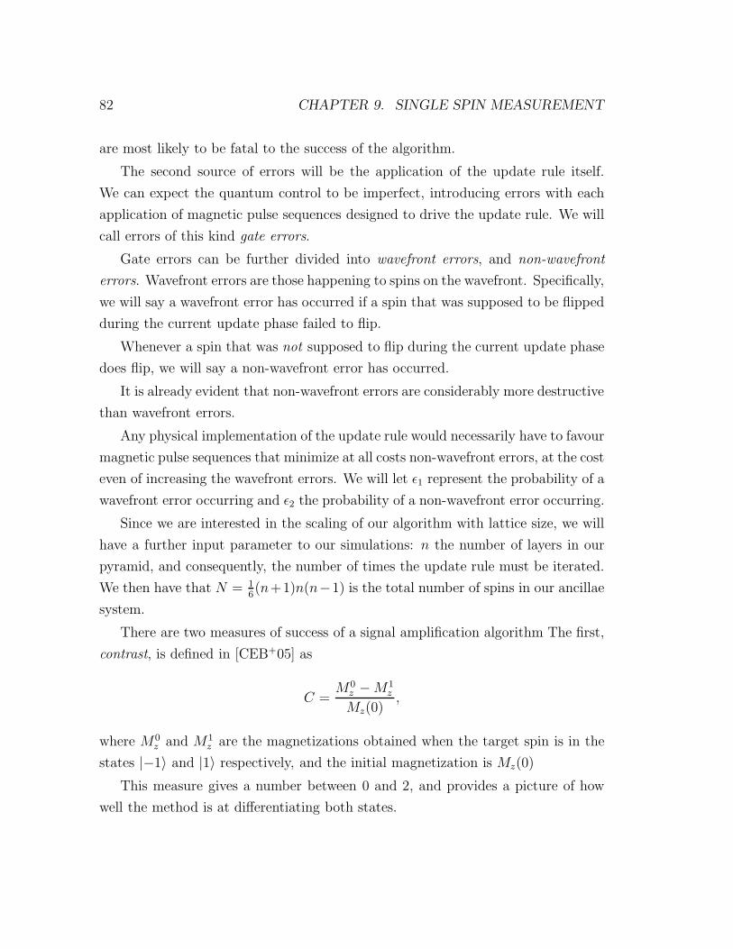
82 CHAPTER 9. SINGLE SPIN MEASUREMENT
are most likely to be fatal to the success of the algorithm.
The second source of errors will be the application of the update rule itself.
We can expect the quantum control to be imperfect, introducing errors with each
application of magnetic pulse sequences designed to drive the update rule. We will
call errors of this kind gate errors.
Gate errors can be further divided into wavefront errors, and non-wavefront
errors. Wavefront errors are those happening to spins on the wavefront. Specifically,
we will say a wavefront error has occurred if a spin that was supposed to be flipped
during the current update phase failed to flip.
Whenever a spin that was not supposed to flip during the current update phase
does flip, we will say a non-wavefront error has occurred.
It is already evident that non-wavefront errors are considerably more destructive
than wavefront errors.
Any physical implementation of the update rule would necessarily have to favour
magnetic pulse sequences that minimize at all costs non-wavefront errors, at the cost
even of increasing the wavefront errors. We will let ǫ1 represent the probability of a
wavefront error occurring and ǫ2 the probability of a non-wavefront error occurring.
Since we are interested in the scaling of our algorithm with lattice size, we will
have a further input parameter to our simulations: n the number of layers in our
pyramid, and consequently, the number of times the update rule must be iterated.
We then have that N = 16(n+1)n(n−1) is the total number of spins in our ancillae
system.
There are two measures of success of a signal amplification algorithm The first,
contrast, is defined in [CEB+05] as
C =M0
z −M1z
Mz(0),
where M0z and M1
z are the magnetizations obtained when the target spin is in the
states |−1〉 and |1〉 respectively, and the initial magnetization is Mz(0)
This measure gives a number between 0 and 2, and provides a picture of how
well the method is at differentiating both states.
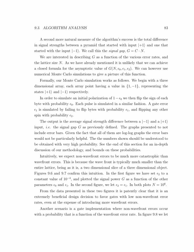
9.3. ALGORITHM ANALYSIS 83
A second more natural measure of the algorithm’s success is the total difference
in signal strengths between a pyramid that started with input |+1〉 and one that
started with the input |−1〉. We call this the signal gap, G = C ·N .
We are interested in describing G as a function of the various error rates, and
the lattice size N . As we have already mentioned it is unlikely that we can achieve
a closed formula for the asymptotic value of G(N, ǫ0, ǫ1, ǫ2). We can however use
numerical Monte Carlo simulations to give a picture of this function.
Formally, our Monte Carlo simulation works as follows. We begin with a three
dimensional array, each array point having a value in 1,−1, representing the
states |+1〉 and |−1〉 respectively.
In order to simulate an initial polarization of 1− ǫ0 we then flip the sign of each
byte with probability ǫ0. Each pulse is simulated in a similar fashion. A gate error
ǫ1 is simulated by failing to flip bytes with probability ǫ1, and flipping any other
spin with probability ǫ2.
The output is the average signal strength difference between a |−1〉 and a |+1〉input, i.e. the signal gap G as previously defined. The graphs presented to not
include error bars. Given the fact that all of them are log-log graphs the error bars
would not be particularly helpful. The the numbers shown should be understood to
be obtained with very high probability. See the end of this section for an in-depth
discussion of our methodology, and bounds on these probabilities.
Intuitively, we expect non-wavefront errors to be much more catastrophic than
wavefront errors. This is because the wave front is typically much smaller than the
entire lattice, being as it is, a two dimensional slice of a three dimensional object.
Figures 9.6 and 9.7 confirm this intuition. In the first figure we have set ǫ2 to a
constant value of 10−4, and plotted the signal power G as a function of the other
parameters ǫ0 and ǫ1. In the second figure, we let ǫ2 = ǫ1. In both plots N = 106.
From the data presented in these two figures it is patently clear that it is an
extremely beneficial design decision to favor gates with low non-wavefront error
rates, even at the expense of introducing more wavefront errors.
Another scenario is a gate implementation where non-wavefront errors occur
with a probability that is a function of the wavefront error rate. In figure 9.8 we let
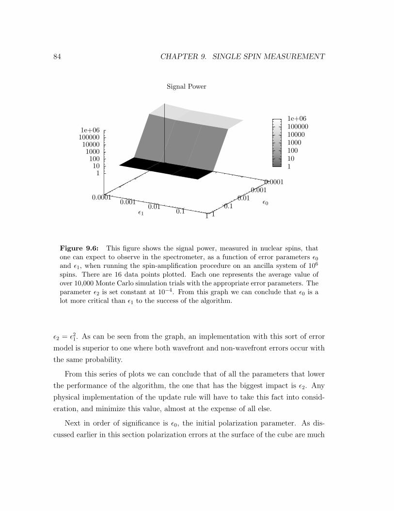
84 CHAPTER 9. SINGLE SPIN MEASUREMENT
1101001000100001000001e+06
Signal Power
0.00010.001
0.010.1
1ǫ1
0.00010.001
0.010.1
1
ǫ0
110
1001000
100001000001e+06
Figure 9.6: This figure shows the signal power, measured in nuclear spins, thatone can expect to observe in the spectrometer, as a function of error parameters ǫ0
and ǫ1, when running the spin-amplification procedure on an ancilla system of 106
spins. There are 16 data points plotted. Each one represents the average value ofover 10,000 Monte Carlo simulation trials with the appropriate error parameters. Theparameter ǫ2 is set constant at 10−4. From this graph we can conclude that ǫ0 is alot more critical than ǫ1 to the success of the algorithm.
ǫ2 = ǫ21. As can be seen from the graph, an implementation with this sort of error
model is superior to one where both wavefront and non-wavefront errors occur with
the same probability.
From this series of plots we can conclude that of all the parameters that lower
the performance of the algorithm, the one that has the biggest impact is ǫ2. Any
physical implementation of the update rule will have to take this fact into consid-
eration, and minimize this value, almost at the expense of all else.
Next in order of significance is ǫ0, the initial polarization parameter. As dis-
cussed earlier in this section polarization errors at the surface of the cube are much
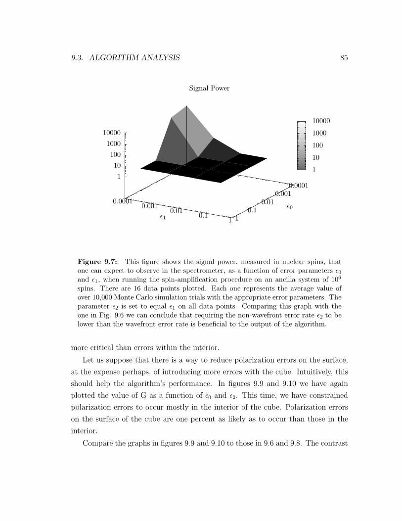
9.3. ALGORITHM ANALYSIS 85
1
10
100
1000
10000
Signal Power
0.00010.001
0.010.1
1ǫ1
0.00010.001
0.010.1
1
ǫ0
1
10
100
1000
10000
Figure 9.7: This figure shows the signal power, measured in nuclear spins, thatone can expect to observe in the spectrometer, as a function of error parameters ǫ0
and ǫ1, when running the spin-amplification procedure on an ancilla system of 106
spins. There are 16 data points plotted. Each one represents the average value ofover 10,000 Monte Carlo simulation trials with the appropriate error parameters. Theparameter ǫ2 is set to equal ǫ1 on all data points. Comparing this graph with theone in Fig. 9.6 we can conclude that requiring the non-wavefront error rate ǫ2 to belower than the wavefront error rate is beneficial to the output of the algorithm.
more critical than errors within the interior.
Let us suppose that there is a way to reduce polarization errors on the surface,
at the expense perhaps, of introducing more errors with the cube. Intuitively, this
should help the algorithm’s performance. In figures 9.9 and 9.10 we have again
plotted the value of G as a function of ǫ0 and ǫ2. This time, we have constrained
polarization errors to occur mostly in the interior of the cube. Polarization errors
on the surface of the cube are one percent as likely as to occur than those in the
interior.
Compare the graphs in figures 9.9 and 9.10 to those in 9.6 and 9.8. The contrast
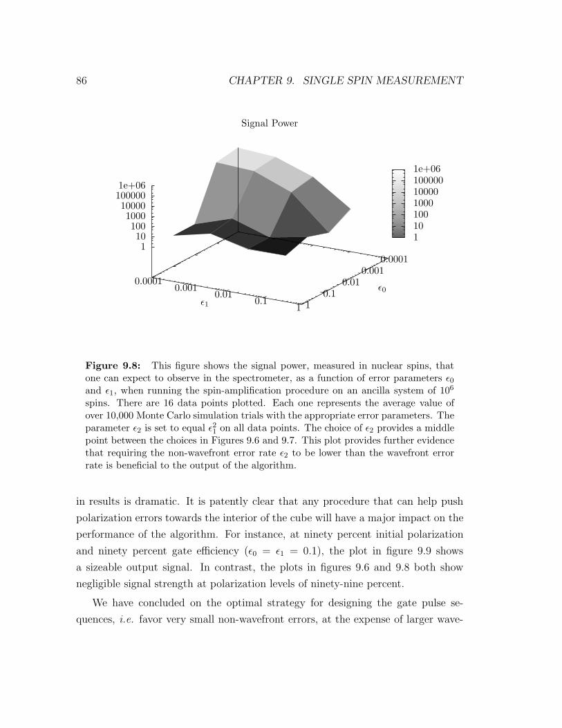
86 CHAPTER 9. SINGLE SPIN MEASUREMENT
1101001000100001000001e+06
Signal Power
0.00010.001
0.010.1
1ǫ1
0.00010.001
0.010.1
1
ǫ0
110
1001000
100001000001e+06
Figure 9.8: This figure shows the signal power, measured in nuclear spins, thatone can expect to observe in the spectrometer, as a function of error parameters ǫ0
and ǫ1, when running the spin-amplification procedure on an ancilla system of 106
spins. There are 16 data points plotted. Each one represents the average value ofover 10,000 Monte Carlo simulation trials with the appropriate error parameters. Theparameter ǫ2 is set to equal ǫ2
1 on all data points. The choice of ǫ2 provides a middlepoint between the choices in Figures 9.6 and 9.7. This plot provides further evidencethat requiring the non-wavefront error rate ǫ2 to be lower than the wavefront errorrate is beneficial to the output of the algorithm.
in results is dramatic. It is patently clear that any procedure that can help push
polarization errors towards the interior of the cube will have a major impact on the
performance of the algorithm. For instance, at ninety percent initial polarization
and ninety percent gate efficiency (ǫ0 = ǫ1 = 0.1), the plot in figure 9.9 shows
a sizeable output signal. In contrast, the plots in figures 9.6 and 9.8 both show
negligible signal strength at polarization levels of ninety-nine percent.
We have concluded on the optimal strategy for designing the gate pulse se-
quences, i.e. favor very small non-wavefront errors, at the expense of larger wave-
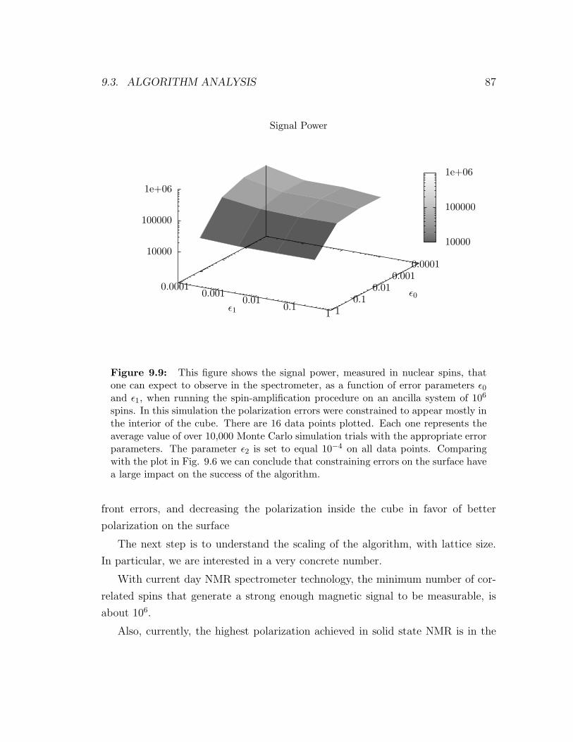
9.3. ALGORITHM ANALYSIS 87
10000
100000
1e+06
Signal Power
0.00010.001
0.010.1
1ǫ1
0.00010.001
0.010.1
1
ǫ0
10000
100000
1e+06
Figure 9.9: This figure shows the signal power, measured in nuclear spins, thatone can expect to observe in the spectrometer, as a function of error parameters ǫ0
and ǫ1, when running the spin-amplification procedure on an ancilla system of 106
spins. In this simulation the polarization errors were constrained to appear mostly inthe interior of the cube. There are 16 data points plotted. Each one represents theaverage value of over 10,000 Monte Carlo simulation trials with the appropriate errorparameters. The parameter ǫ2 is set to equal 10−4 on all data points. Comparingwith the plot in Fig. 9.6 we can conclude that constraining errors on the surface havea large impact on the success of the algorithm.
front errors, and decreasing the polarization inside the cube in favor of better
polarization on the surface
The next step is to understand the scaling of the algorithm, with lattice size.
In particular, we are interested in a very concrete number.
With current day NMR spectrometer technology, the minimum number of cor-
related spins that generate a strong enough magnetic signal to be measurable, is
about 106.
Also, currently, the highest polarization achieved in solid state NMR is in the
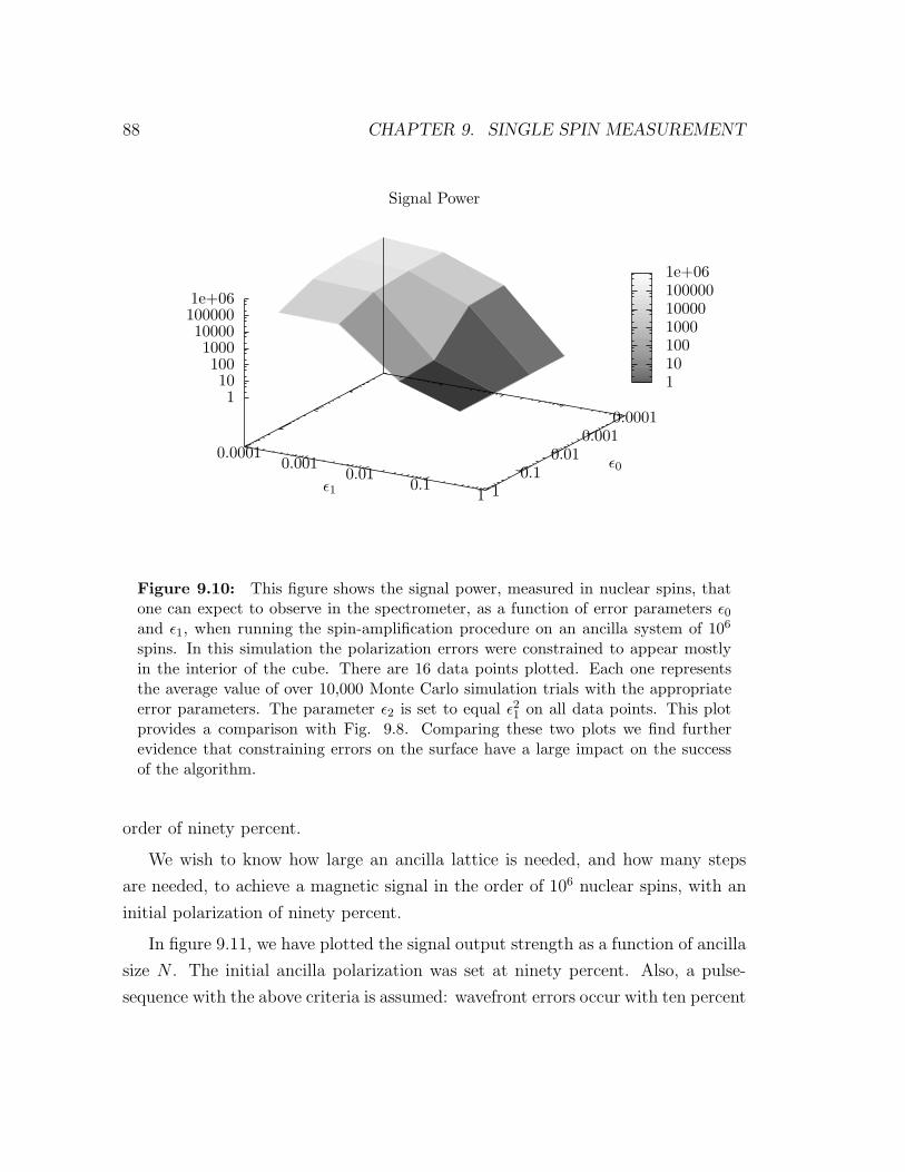
88 CHAPTER 9. SINGLE SPIN MEASUREMENT
1101001000100001000001e+06
Signal Power
0.00010.001
0.010.1
1ǫ1
0.00010.001
0.010.1
1
ǫ0
110
1001000
100001000001e+06
Figure 9.10: This figure shows the signal power, measured in nuclear spins, thatone can expect to observe in the spectrometer, as a function of error parameters ǫ0
and ǫ1, when running the spin-amplification procedure on an ancilla system of 106
spins. In this simulation the polarization errors were constrained to appear mostlyin the interior of the cube. There are 16 data points plotted. Each one representsthe average value of over 10,000 Monte Carlo simulation trials with the appropriateerror parameters. The parameter ǫ2 is set to equal ǫ2
1 on all data points. This plotprovides a comparison with Fig. 9.8. Comparing these two plots we find furtherevidence that constraining errors on the surface have a large impact on the successof the algorithm.
order of ninety percent.
We wish to know how large an ancilla lattice is needed, and how many steps
are needed, to achieve a magnetic signal in the order of 106 nuclear spins, with an
initial polarization of ninety percent.
In figure 9.11, we have plotted the signal output strength as a function of ancilla
size N . The initial ancilla polarization was set at ninety percent. Also, a pulse-
sequence with the above criteria is assumed: wavefront errors occur with ten percent
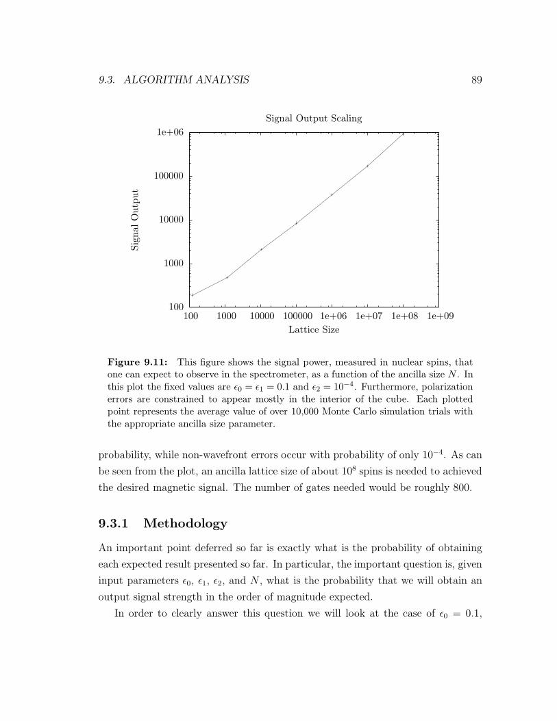
9.3. ALGORITHM ANALYSIS 89
100
1000
10000
100000
1e+06
100 1000 10000 100000 1e+06 1e+07 1e+08 1e+09
Sig
nal
Outp
ut
Lattice Size
Signal Output Scaling
Figure 9.11: This figure shows the signal power, measured in nuclear spins, thatone can expect to observe in the spectrometer, as a function of the ancilla size N . Inthis plot the fixed values are ǫ0 = ǫ1 = 0.1 and ǫ2 = 10−4. Furthermore, polarizationerrors are constrained to appear mostly in the interior of the cube. Each plottedpoint represents the average value of over 10,000 Monte Carlo simulation trials withthe appropriate ancilla size parameter.
probability, while non-wavefront errors occur with probability of only 10−4. As can
be seen from the plot, an ancilla lattice size of about 108 spins is needed to achieved
the desired magnetic signal. The number of gates needed would be roughly 800.
9.3.1 Methodology
An important point deferred so far is exactly what is the probability of obtaining
each expected result presented so far. In particular, the important question is, given
input parameters ǫ0, ǫ1, ǫ2, and N , what is the probability that we will obtain an
output signal strength in the order of magnitude expected.
In order to clearly answer this question we will look at the case of ǫ0 = 0.1,
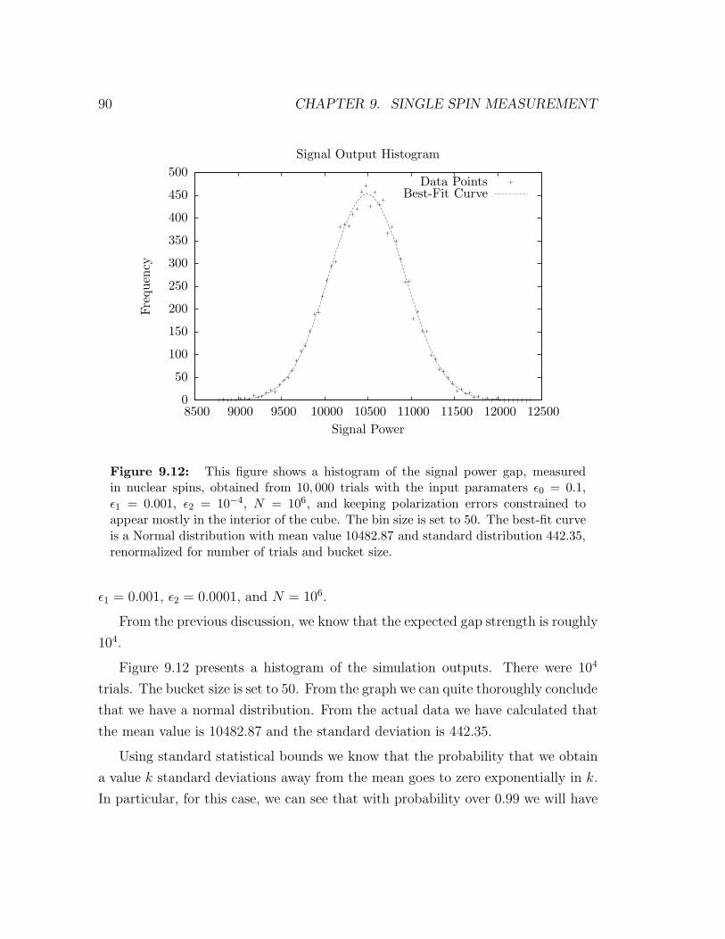
90 CHAPTER 9. SINGLE SPIN MEASUREMENT
0
50
100
150
200
250
300
350
400
450
500
8500 9000 9500 10000 10500 11000 11500 12000 12500
Fre
quen
cy
Signal Power
Signal Output Histogram
Data PointsBest-Fit Curve
Figure 9.12: This figure shows a histogram of the signal power gap, measuredin nuclear spins, obtained from 10, 000 trials with the input paramaters ǫ0 = 0.1,ǫ1 = 0.001, ǫ2 = 10−4, N = 106, and keeping polarization errors constrained toappear mostly in the interior of the cube. The bin size is set to 50. The best-fit curveis a Normal distribution with mean value 10482.87 and standard distribution 442.35,renormalized for number of trials and bucket size.
ǫ1 = 0.001, ǫ2 = 0.0001, and N = 106.
From the previous discussion, we know that the expected gap strength is roughly
104.
Figure 9.12 presents a histogram of the simulation outputs. There were 104
trials. The bucket size is set to 50. From the graph we can quite thoroughly conclude
that we have a normal distribution. From the actual data we have calculated that
the mean value is 10482.87 and the standard deviation is 442.35.
Using standard statistical bounds we know that the probability that we obtain
a value k standard deviations away from the mean goes to zero exponentially in k.
In particular, for this case, we can see that with probability over 0.99 we will have
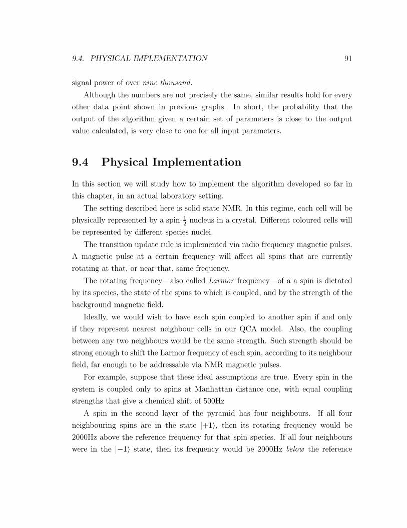
9.4. PHYSICAL IMPLEMENTATION 91
signal power of over nine thousand.
Although the numbers are not precisely the same, similar results hold for every
other data point shown in previous graphs. In short, the probability that the
output of the algorithm given a certain set of parameters is close to the output
value calculated, is very close to one for all input parameters.
9.4 Physical Implementation
In this section we will study how to implement the algorithm developed so far in
this chapter, in an actual laboratory setting.
The setting described here is solid state NMR. In this regime, each cell will be
physically represented by a spin-12
nucleus in a crystal. Different coloured cells will
be represented by different species nuclei.
The transition update rule is implemented via radio frequency magnetic pulses.
A magnetic pulse at a certain frequency will affect all spins that are currently
rotating at that, or near that, same frequency.
The rotating frequency—also called Larmor frequency—of a a spin is dictated
by its species, the state of the spins to which is coupled, and by the strength of the
background magnetic field.
Ideally, we would wish to have each spin coupled to another spin if and only
if they represent nearest neighbour cells in our QCA model. Also, the coupling
between any two neighbours would be the same strength. Such strength should be
strong enough to shift the Larmor frequency of each spin, according to its neighbour
field, far enough to be addressable via NMR magnetic pulses.
For example, suppose that these ideal assumptions are true. Every spin in the
system is coupled only to spins at Manhattan distance one, with equal coupling
strengths that give a chemical shift of 500Hz
A spin in the second layer of the pyramid has four neighbours. If all four
neighbouring spins are in the state |+1〉, then its rotating frequency would be
2000Hz above the reference frequency for that spin species. If all four neighbours
were in the |−1〉 state, then its frequency would be 2000Hz below the reference
92 CHAPTER 9. SINGLE SPIN MEASUREMENT
Figure 9.13: This is the ideal spectrum for a spin on the second layer. There are5 distinct peaks, one for each of the five neighbour field values. Having a spectra ofthis type implies we can selectively update the desired spins without inadvertentlychanging the state of spins that should remain unchanged.
frequency. With equal neighbours pointing up and down, the spin would resonate
at exactly the reference frequency, and so on.
One way to graphically present this information is by giving a spin’s spectrum.
In this case we will give a simulated spectrum. We take a spin, with four neighbours,
in the conditions outlined above. We put the neighbours in the completely mixed
state. If we were to measure magnetic signals at and around the reference frequency,
we would see five peaks: one for each of the conditions outlined above. Figure 9.13
showcases this simulated spectrum.
This is an ideal situation. Each neighbour field gives one distinct frequency peak,
clearly defined and separated from the other peaks. Also, we have the advantage
that the neighbour fields we wish to affect, namely −2, −1 and 0, are all packed
together.
Unfortunately, we do not get to choose the Hamiltonian of our system. In our
case, we are constrained to using the Dipole-Dipole coupling Hamiltinian:
H =∑
i<j
di,j
[σi
zσjz − ki,j
(σi
+σj− + σi
−σj+
)], (9.1)
9.4. PHYSICAL IMPLEMENTATION 93
where ki,j equals one if i, j are of the same species and zero otherwise;
di,j =gi,j
r3i,j
1
2
(3 cos2 Θi,j − 1
)= ωd
r3i,i+1
r3i,j
, (9.2)
where ri,j is the distance between the two nuclei, Θi,j is the angle between the
vector connecting the two nuclei and the z- axis (determined by the magnetic field)
and gi,j is a simple constant that depends only on the nuclear types of i and j.
There are two obvious obstacles we need to address before we can attempt to
use a system with this Hamiltonian as our spin signal amplification ancilla.
The first thing to note is that the Hamiltonian is not nearest neighbour coupling
only. Essentially, every spin is coupled to every other spin in the crystal. The state
of every single spin has the propensity to shift the rotating frequency of every other
spin in the system.
The second obstacle is that a priori there is no guarantee that the couplings be-
tween nearest neighbours will all be of the same strength. Notice that the coupling
strength depends on two factors: the distance r between the two spins, and the
angle Θ between the vector that joins them, and the z-axis of the strong magnetic
field.
The solution to this second problem is easier, so we will tackle it first. We can
orient the crystal inside the NMR probe in any fashion we see fit. By orienting the
crystal so that the top layer is pointing up, we can guarantee that the angle Θ is
equal for all neighbours in our scheme. This however, means that we cannot use a
cubic crystal. The reason for this is that if we orient a perfect cube in such fashion
then the angle Θ for nearest neighbours becomes arctan√
2, a number known as the
magic angle. It is known as such for its property, that if substituted into equation
9.2 above, it makes the coupling strength equal to zero.
This in itself is not a major roadblock, but rather just something we need to
keep in mind. It is possible to use different crystal structures. About any crystal
structure will work well, as long as the Bravais angles, the angles formed edges of
the crystal, are significantly different from ninety degrees. For our purposes we will
from now assume a rombohedral crystal with Bravais angles of sixty degrees.
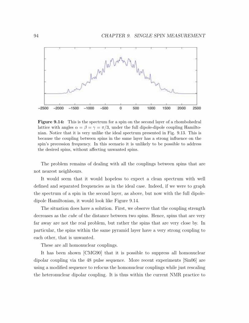
94 CHAPTER 9. SINGLE SPIN MEASUREMENT
Figure 9.14: This is the spectrum for a spin on the second layer of a rhombohedrallattice with angles α = β = γ = π/3, under the full dipole-dipole coupling Hamilto-nian. Notice that it is very unlike the ideal spectrum presented in Fig. 9.13. This isbecause the coupling between spins in the same layer has a strong influence on thespin’s precession frequency. In this scenario it is unlikely to be possible to addressthe desired spins, without affecting unwanted spins.
The problem remains of dealing with all the couplings between spins that are
not nearest neighbours.
It would seem that it would hopeless to expect a clean spectrum with well
defined and separated frequencies as in the ideal case. Indeed, if we were to graph
the spectrum of a spin in the second layer, as above, but now with the full dipole-
dipole Hamiltonian, it would look like Figure 9.14.
The situation does have a solution. First, we observe that the coupling strength
decreases as the cube of the distance between two spins. Hence, spins that are very
far away are not the real problem, but rather the spins that are very close by. In
particular, the spins within the same pyramid layer have a very strong coupling to
each other, that is unwanted.
These are all homonuclear couplings.
It has been shown [CMG90] that it is possible to suppress all homonuclear
dipolar coupling via the 48 pulse sequence. More recent experiments [Sin06] are
using a modified sequence to refocus the homonuclear couplings while just rescaling
the heteronuclear dipolar coupling. It is thus within the current NMR practice to
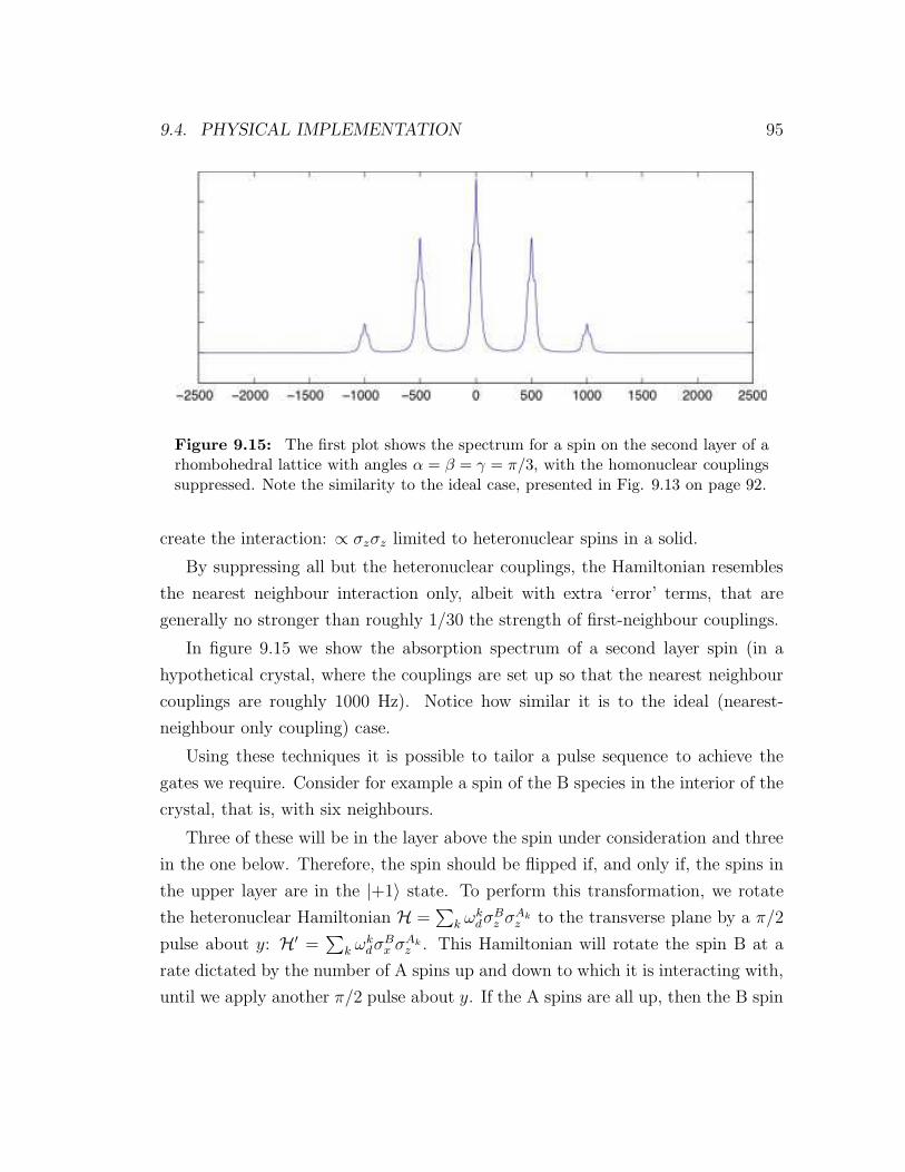
9.4. PHYSICAL IMPLEMENTATION 95
Figure 9.15: The first plot shows the spectrum for a spin on the second layer of arhombohedral lattice with angles α = β = γ = π/3, with the homonuclear couplingssuppressed. Note the similarity to the ideal case, presented in Fig. 9.13 on page 92.
create the interaction: ∝ σzσz limited to heteronuclear spins in a solid.
By suppressing all but the heteronuclear couplings, the Hamiltonian resembles
the nearest neighbour interaction only, albeit with extra ‘error’ terms, that are
generally no stronger than roughly 1/30 the strength of first-neighbour couplings.
In figure 9.15 we show the absorption spectrum of a second layer spin (in a
hypothetical crystal, where the couplings are set up so that the nearest neighbour
couplings are roughly 1000 Hz). Notice how similar it is to the ideal (nearest-
neighbour only coupling) case.
Using these techniques it is possible to tailor a pulse sequence to achieve the
gates we require. Consider for example a spin of the B species in the interior of the
crystal, that is, with six neighbours.
Three of these will be in the layer above the spin under consideration and three
in the one below. Therefore, the spin should be flipped if, and only if, the spins in
the upper layer are in the |+1〉 state. To perform this transformation, we rotate
the heteronuclear Hamiltonian H =∑
k ωkdσ
Bz σ
Akz to the transverse plane by a π/2
pulse about y: H′ =∑
k ωkdσ
Bx σ
Akz . This Hamiltonian will rotate the spin B at a
rate dictated by the number of A spins up and down to which it is interacting with,
until we apply another π/2 pulse about y. If the A spins are all up, then the B spin
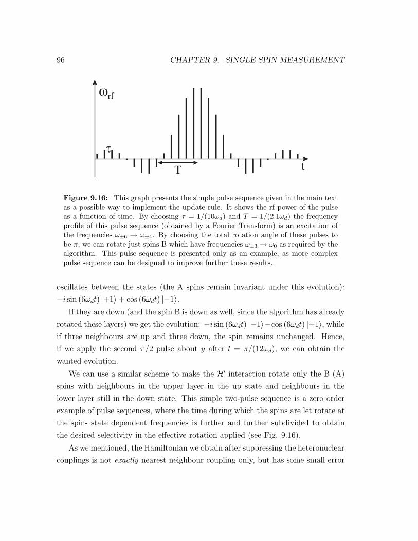
96 CHAPTER 9. SINGLE SPIN MEASUREMENT
τ
Τt
ωrf
Figure 9.16: This graph presents the simple pulse sequence given in the main textas a possible way to implement the update rule. It shows the rf power of the pulseas a function of time. By choosing τ = 1/(10ωd) and T = 1/(2.1ωd) the frequencyprofile of this pulse sequence (obtained by a Fourier Transform) is an excitation ofthe frequencies ω±6 → ω±4. By choosing the total rotation angle of these pulses tobe π, we can rotate just spins B which have frequencies ω±3 → ω0 as required by thealgorithm. This pulse sequence is presented only as an example, as more complexpulse sequence can be designed to improve further these results.
oscillates between the states (the A spins remain invariant under this evolution):
−i sin (6ωdt) |+1〉 + cos (6ωdt) |−1〉.If they are down (and the spin B is down as well, since the algorithm has already
rotated these layers) we get the evolution: −i sin (6ωdt) |−1〉−cos (6ωdt) |+1〉, while
if three neighbours are up and three down, the spin remains unchanged. Hence,
if we apply the second π/2 pulse about y after t = π/(12ωd), we can obtain the
wanted evolution.
We can use a similar scheme to make the H′ interaction rotate only the B (A)
spins with neighbours in the upper layer in the up state and neighbours in the
lower layer still in the down state. This simple two-pulse sequence is a zero order
example of pulse sequences, where the time during which the spins are let rotate at
the spin- state dependent frequencies is further and further subdivided to obtain
the desired selectivity in the effective rotation applied (see Fig. 9.16).
As we mentioned, the Hamiltonian we obtain after suppressing the heteronuclear
couplings is not exactly nearest neighbour coupling only, but has some small error
9.4. PHYSICAL IMPLEMENTATION 97
terms. These error terms, as well as imperfect control, will cause imperfect gates.
Also, the crystal lattice may not be perfectly polarized initially. It is important to
deal with these issues.
As we have already mentioned our scheme is impervious to phase-flip errors in
the lattice. Effectively, all pulses, and the final output, depend only on the diagonal
terms of the density operator ρ of the lattice.
We have already mentioned rudimentary methods for bit-flip tolerance in the
previous section.
We mentioned that errors inside the pyramid are less critical than errors on the
faces, or worse, edges, of the pyramid.
The reason is that inside the pyramid all lattice points have exactly 6 neighbours.
If one flips erroneously, there are still 5 neighbours in the correct state.
Previously we concluded that we need to suppress the homonuclear coupling
during our pulse sequences. In this Hamiltonian, the term σi+σ
j− + σi
−σj+, often
referred to as the ‘flip-flop’ term, has the effect of swapping two anti-aligned neigh-
bouring spins. Take a horizontal slice of the pyramid and suppose there is a single
error among these lattice points. The effect of the flip-flop term on neighbouring
spins is well known and is called spin diffusion [Wau98]. A simple approximation
to this dynamics is a quantum walk on the lattice. In this model, an erroneous
bit not only becomes diffused over several spins, it also has a much lower proba-
bility (averaged over time) of being in non-interior points. This leads us to believe
that letting the system evolve under the homonuclear interaction for some time
before running the algorithm will have the effect of reducing errors in the edges,
and increase overall robustness to errors.

Chapter 10
Further Directions and
Conclusions
We will begin this final chapter by discussing some of the research directions opened
by the results in the preceding. We will discuss what progress has been made in
these directions, if any. We will also discuss open problems in this area of research.
Insight will be provided into how one may tackle resolving such questions.
In many cases, the ideas presented here represent current work in progress.
Although a complete formal resolution was not available at the time of this writing,
a clear intuitive picture is present. Other ideas presented here are more speculative
in nature.
We will close this chapter, and this thesis, with a summary of results, and some
closing remarks from this author.
10.1 Dissipative QCA
The model of QCA we have introduced and discussed throughout this thesis is
based solely on unitary evolution steps.
In many cases, this is all that is needed. For many physical systems, all inter-
actions are constrained to nearest, or next nearest neighbours. In these cases, the
LUQCA accounts for all types of evolution.
99
100 CHAPTER 10. FURTHER DIRECTIONS AND CONCLUSIONS
Consider however, the situation where not all interactions are constrained to
being between lattice cells.
For example, one might contemplate a quantum system consisting of homoge-
nous subsystems, with nearest neighbour couplings—as in traditional QCA—but
with the added factor of a coupling between each subsystem and some external one:
a gradient magnetic field, some vibrational degree of freedom, etc.
As discussed previously, in many cases it is not difficult to consider this external
force as part of the QCA model. In many other cases, it might not be as easy, or
even beneficial to do so.
In particular, consider the case of a solid-state NMR quantum computer. This
could be constructed using some crystalline structure where each spin-12
nucleus is a
register in the quantum computer. Since normally we would not expect individual
control of these registers, but only selective global control, this is an ideal case for
QCA modelling.
However, let us further suppose that the coupling between the nuclei and the
electron spins—called the hyperfine interaction—is used to reduce the entropy of
the nuclear spin registers both before (cooling) and during (quantum error correc-
tion) the computation. This procedure would take advantage of the much shorter
relaxation times of the electrons, compared to the nuclear spins.
The electron spins are not considered as part of the quantum computer proper,
they are simply a mechanism for enhancing the control of it.
In such case, we may wish to model the quantum computer as a QCA, or
implement a QCA algorithm on it. However, the fact that it is not a closed quantum
system means we can no longer restrict our attention to unitary evolution.
What we want to add to our model is the ability to consider couplings between
lattice cells and some external system—environment, heat bath, etc. A simple way
to do this is to extend the definition of our local update rule to allow the update step
V , to be a general completely-positive trace preserving (CPTP) map. Formally,
Definition 10.1. A Dissipative Quantum Cellular Automaton (QCA) is a 5-tuple
(L,Σ,N , U0, V0) consisting of a d-dimensional lattice of cells indexed by integers,
L = Zd, a finite set Σ of orthogonal basis states, a finite neighbourhood scheme
10.1. DISSIPATIVE QCA 101
N ⊆ Zd, a local read function U0 ∈ U(H⊗N
Σ
), and a local update function V0 ∈
A (HΣ). The read operation carries the further restriction that any two lattice
translations Ux and Uy must commute for all x, y ∈ L.
As with LUQCA, each cell has a finite Hilbert space associated with it HΣ =
span (Σ). The reduced state of each cell is a density operator over this Hilbert
space ρx ∈ D (HΣ).
The main difference between dissipative and non-dissipitative QCA lies in the
definition of the local update rule V0. Recall that in LUQCA V0 was defined to
be a unitary operator, acting on the Hilbert space of a single cell, while here V0 is
defined a CPTP map mapping the space of a single cell onto itself V0 ∈ A (HΣ).
Likewise, we extend the definition of the initial state of the QCA to allow for ar-
bitrary density operators, instead of allowing only pure initial state configurations.
Formally, the initial state of a dissipitative QCA is defined in the following way.
Let f be any computable function that maps lattice vectors to density operators
ρ ∈ D(H⊗kd
Σ
), where d is the dimension of the QCA lattice, and k is the block size of
the initial state. Then for any lattice vector z = (z1k, z2k, . . . , zdk) ∈ Zd the initial
state of the lattice hypercube delimited by (z1k, z2k, . . . , zdk) and ((z + 1)k − 1,
(z1 + 1)k − 1, . . . , (zd + 1)k − 1) is set to f(z).
We can mention some results regarding this extended model.
First, it is obvious that LUQCA constitute a proper subset of DQCA. However,
we also know that LUQCA are universal for quantum computation, and that quan-
tum computation is Turing complete. This means that for every DQCA there must
be an LUQCA that can simulate it.
However, this does not imply that this simulation be in any way efficient. This
is in fact, an open problem left by this thesis: Does there exist an efficient—in
dimensions, number of states, and number of steps—simulation of any DQCA in
the LUQCA model?
If the question were to be answered in the affirmative this would seem to imply,
inter alia, that general algorithmic cooling is as efficient with, or without, a heat
bath. Given results to the contrary [SMW07,SMW05], it seems unlikely that this
would be the case. Hence a conjecture put forth in this thesis is that in fact there
102 CHAPTER 10. FURTHER DIRECTIONS AND CONCLUSIONS
exists no such efficient simulation.
Two important applications of DQCA are exporing algorithmic cooling, and
fault-tolerant QCA.
10.1.1 Algorithmic Cooling with QCA
Algorithmic cooling is a procedure by which a subsystem s of a much larger system
S is ‘cooled down’, i.e. its entropy reduced by applying unitary operations on the
system S. This of course has the side effect of increasing the entropy on the system
S \ s, a necessary condition to ensure consistency with thermodynamics.
Two different formalizations exist. The first one [SV99] considers the whole
system S as a computational resource with a computational cost associated with
it. For instance, the cooler we want the qubits in the subsystem s to be, the larger
the system S \ s, and by consequence the system S as a whole, have to be.
The second formalization [SMW05,SMW07] does not consider the system S \ sto be part of the computer itself, but regards it as an exernal heat bath. The
system S \ s is seen as a pontentially infinite reservoir from which cool qubits can
be drawn, and to which hot qubits can be sent, without ever noticeably changing
its temperature.
Both formalizations are valid, and reasonable under differing assumptions. While
it may seem that algorithmic cooling algorithms with access to a heat bath are more
efficient than those without, this is not entirely true. Part, if not all, of this appar-
ent gain in efficiency is a consequence of not formally accounting for all resources
used. This is not to say, that with regards to some specific experimental setups,
this heat bath can be seen as a potentially infinite reservoir of ‘coolness’.
A very clear and concise description of major algorithmic cooling algorithms,
both with and without a heat bath, is given in [Kay07b].
All algorithmic cooling algorithms can be described simply as follows.
Suppose we start with a set S of qubits all in the state:
1 + ǫ02
|0〉 〈0| + 1 − ǫ02
|1〉 〈1| .
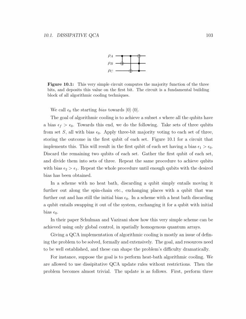
10.1. DISSIPATIVE QCA 103
ρA • •
ρB •ρC •
Figure 10.1: This very simple circuit computes the majority function of the threebits, and deposits this value on the first bit. The circuit is a fundamental buildingblock of all algorithmic cooling techniques.
We call ǫ0 the starting bias towards |0〉 〈0|.The goal of algorithmic cooling is to achieve a subset s where all the qubits have
a bias ǫf > ǫ0. Towards this end, we do the following. Take sets of three qubits
from set S, all with bias ǫ0. Apply three-bit majority voting to each set of three,
storing the outcome in the first qubit of each set. Figure 10.1 for a circuit that
implements this. This will result in the first qubit of each set having a bias ǫ1 > ǫ0.
Discard the remaining two qubits of each set. Gather the first qubit of each set,
and divide them into sets of three. Repeat the same procedure to achieve qubits
with bias ǫ2 > ǫ1. Repeat the whole procedure until enough qubits with the desired
bias has been obtained.
In a scheme with no heat bath, discarding a qubit simply entails moving it
further out along the spin-chain etc., exchanging places with a qubit that was
further out and has still the initial bias ǫ0. In a scheme with a heat bath discarding
a qubit entails swapping it out of the system, exchanging it for a qubit with initial
bias ǫ0.
In their paper Schulman and Vazirani show how this very simple scheme can be
achieved using only global control, in spatially homogenous quantum arrays.
Giving a QCA implementation of algorithmic cooling is mostly an issue of defin-
ing the problem to be solved, formally and extensively. The goal, and resources need
to be well established, and these can shape the problem’s difficulty dramatically.
For instance, suppose the goal is to perform heat-bath algorithmic cooling. We
are allowed to use dissipitative QCA update rules without restrictions. Then the
problem becomes almost trivial. The update is as follows. First, perform three
104 CHAPTER 10. FURTHER DIRECTIONS AND CONCLUSIONS
bit-majority on every set of three contiguous cells, storing the result in the first
cell. Then reset the second and third cells with the heat-bath.
The problem becomes slightly harder if we only allow a few special cells to
interact with the heat-bath. However, this can still be done as long as one is allowed
to use extra workspace within each cell (not target of the cooling algorithm). This
extra space can be used to encode clock-registers and so on needed to perform a
simulation of the GCQA cooling algorithm proposed b Schulman and Vazirani.
The problem becomes a lot more difficult if we are assuming that each cell
consists only of a single qubit, which is to be cooled. In this case, there is no way
to perform a time-dependant evolution. In fact, without using Coloured QCA in
order to provide spatial distinguishability, the problem might even be intractable.
It is possible that using a Coloured Dissipitative QCA one could design an
algorithm that performs cooling throughout the lattice, without the need for time-
dependancies in the update rule. Providing such an algorithm is work in progress.
10.1.2 Fault-Tolerant QCA
Fault-tolerant quantum computing is an issue that has been well addressed in the
general circuit model [CS96,Got98,Got07], in the local-gate circuit model [STD05],
and more recently in globally controlled quantum arrays [BBK03,Kay05,Kay07a,
FT07].
It is unclear how well these fault tolerance methods could be translated into the
QCA model. In particular the scheme presented in [FT07] requires a highly non-
space homogenous array, not to mention time inhomogeneity. While it is possible,
as has been shown extensively throughout this thesis, to simulate non-homogenous
systems on QCA, here we are presented with a much more challenging problem.
In simulating any of these fault-tolerant schemes within the QCA model, it is
important to prove that the constructions upon which the simulation is constructed
on, are themselves, fault tolerant. Summarily, it is not enough to simply give a
simulation of a fault-tolerant circuit in the QCA model, it is necessary to show that
way the simulation is built is fault-tolerant as well.
It is possible that the road towards fault tolerant QCA lies not in looking for
10.2. FURTHER PHYSICAL IMPLEMENTATIONS OF QCA 105
such simulation, but in building a fault-tolerant QCA from the ground up. In order
to do this, one may try to learn the lessons learned in building a classical fault
tolerant CA [Gac83].
Peter Gacs [Gac83] gives a construction, along with a complete description, of
a fully functional classical fault-tolerant CA. The complexity of his construction,
makes the prospect of emulating his work in the quantum regime extremely daunt-
ing.
10.2 Further Physical Implementations of QCA
In Chapter 8 we studied solid-state NMR as quantum computing architecture that
is ideal for implementing QCA algorithms.
Many other proposal for universal quantum computer implementations have
been proposed. Of these, any such where addressing a single qubit is a major
concern, while concatenating a large number of them is not, would seem to be an
ideal candidate for a QCA approach.
Buckyballs in nanotubes [BAB+06] is very interesting example of such a system.
Any generalization of the systems described therein, e.g. general doped organic
structures in up to three dimension would also be prime candidates.
10.3 Modifications and Further Applications of
Spin-Amplification
In Chapter 9 we discussed the ‘Pyramid Scheme’ spin-amplification algorithm. We
mentioned that the main application of such an algorithm is to act as a measurement
device. In this section we will see how to further this application, as well as give a
different, but related, application.
106 CHAPTER 10. FURTHER DIRECTIONS AND CONCLUSIONS
10.3.1 Using Different Lattice Structures
Perhaps one of the biggest avenues for further research on spin-amplification is
adapting the algorithm for different lattice structures.
The choice of lattice structure in Chapter 9 was very careful and deliberate one.
The A−B chess-grid structure provides a simple enough environment, yet powerful
enough to implement the algorithm. At the same time, it is not unreasonable
to expect a crystal with said structure to be made available, either naturally or
artificially, for the purposes of said algorithm.
There are, however, many reasons to consider alternative lattices.
First, so far an ideal candidate crystal has not been found with the above lattice
structure. If a crystal which is otherwise appropriate, but with a different crystal
lattice structure, were to be found, implementing the algorithm on such lattice
would become of utmost priority.
There is also the prospect of implementing spin-amplfication in different quan-
tum hardware, not necessarily solid-state NMR. For instance, one may wish to
implement the algorithm using ESR on different molecules. Buckyballs, nan-
otubes [BAB+06], polymers, all represent viable candidates for implementing spin-
amplification, and each would require a different approach.
10.3.2 Cat State Creation and Verification
Here we discuss another application of the algorithm: the creation and verification
of large ‘cat’ states.
Ever since Schrodinger [Sch35] noted that quantum mechanics allows for super-
positions of arbitrarily large, even macroscopic, systems, e.g. cats, there has been
a myriad of experiments, and experiment proposals for generating ever larger ‘Cat
States’. One purpose of such experiments is to better understand decoherence, and
the transition from quantum to classical.
There are several examples of experimental realizations of cat states. For in-
stance, the Bucky Ball (C60) interferometer [ANVA+99]. Their experimental setup
is similar to the well known Young’s double-slit experiment, except that it uses
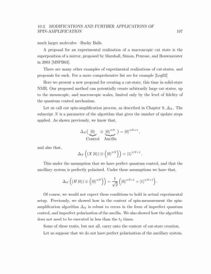
10.3. MODIFICATIONS AND FURTHER APPLICATIONS OF
SPIN-AMPLIFICATION 107
much larger molecules—Bucky Balls.
A proposal for an experimental realization of a macroscopic cat state is the
superposition of a mirror, proposed by Marshall, Simon, Penrose, and Bouwmeester
in 2003 [MSPB03].
There are many other examples of experimental realizations of cat-states, and
proposals for such. For a more comprehensive list see for example [Leg02]
Here we present a new proposal for creating a cat-state, this time in solid-state
NMR. Our proposed method can potentially create arbitrarily large cat states, up
to the mesoscopic, and macroscopic scales, limited only by the level of fidelity of
the quantum control mechanism.
Let us call our spin-amplification process, as described in Chapter 9, ∆N . The
subscript N is a parameter of the algorithm that gives the number of update steps
applied. As shown previously, we know that,
∆N
(|0〉︸︷︷︸
Control
⊗ |0〉⊗N
︸ ︷︷ ︸Ancilla
)= |0〉⊗N+1 ,
and also that,
∆N
((X |0〉) ⊗
(|0〉⊗N
))= |1〉⊗N+1 .
This under the assumption that we have perfect quantum control, and that the
ancillary system is perfectly polarized. Under these assumptions we have that,
∆N
((H |0〉) ⊗
(|0〉⊗N
))=
1√2
(|0〉⊗N+1 + |1〉⊗N+1
).
Of course, we would not expect these conditions to hold in actual experimental
setup. Previously, we showed how in the context of spin-measurement the spin-
amplification algorithm ∆N is robust to errors in the form of imperfect quantum
control, and imperfect polarization of the ancilla. We also showed how the algorithm
does not need to be executed in less than the t2 times.
Some of these traits, but not all, carry onto the context of cat-state creation.
Let us suppose that we do not have perfect polarization of the ancillary system.
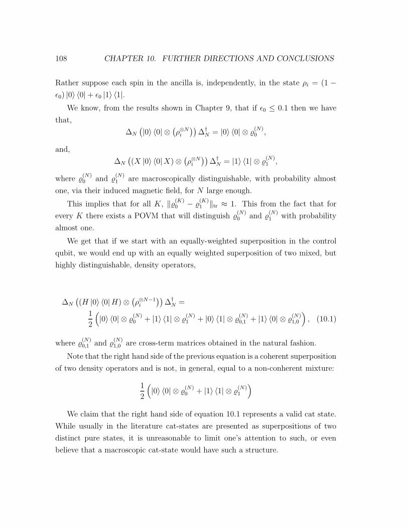
108 CHAPTER 10. FURTHER DIRECTIONS AND CONCLUSIONS
Rather suppose each spin in the ancilla is, independently, in the state ρi = (1 −ǫ0) |0〉 〈0| + ǫ0 |1〉 〈1|.
We know, from the results shown in Chapter 9, that if ǫ0 ≤ 0.1 then we have
that,
∆N
(|0〉 〈0| ⊗
(ρ⊗N
i
))Ơ
N = |0〉 〈0| ⊗ (N)0 ,
and,
∆N
((X |0〉 〈0|X) ⊗
(ρ⊗N
i
))Ơ
N = |1〉 〈1| ⊗ (N)1 ,
where (N)0 and
(N)1 are macroscopically distinguishable, with probability almost
one, via their induced magnetic field, for N large enough.
This implies that for all K, ‖(K)0 −
(K)1 ‖tr ≈ 1. This from the fact that for
every K there exists a POVM that will distinguish (N)0 and
(N)1 with probability
almost one.
We get that if we start with an equally-weighted superposition in the control
qubit, we would end up with an equally weighted superposition of two mixed, but
highly distinguishable, density operators,
∆N
((H |0〉 〈0|H) ⊗
(ρ⊗N−1
i
))Ơ
N =
1
2
(|0〉 〈0| ⊗
(N)0 + |1〉 〈1| ⊗
(N)1 + |0〉 〈1| ⊗
(N)0,1 + |1〉 〈0| ⊗
(N)1,0
), (10.1)
where (N)0,1 and
(N)1,0 are cross-term matrices obtained in the natural fashion.
Note that the right hand side of the previous equation is a coherent superposition
of two density operators and is not, in general, equal to a non-conherent mixture:
1
2
(|0〉 〈0| ⊗
(N)0 + |1〉 〈1| ⊗
(N)1
)
We claim that the right hand side of equation 10.1 represents a valid cat state.
While usually in the literature cat-states are presented as superpositions of two
distinct pure states, it is unreasonable to limit one’s attention to such, or even
believe that a macroscopic cat-state would have such a structure.
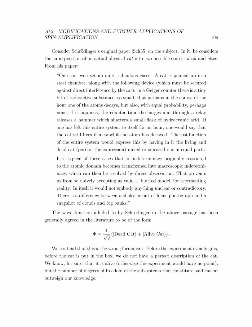
10.3. MODIFICATIONS AND FURTHER APPLICATIONS OF
SPIN-AMPLIFICATION 109
Consider Schrodinger’s original paper [Sch35] on the subject. In it, he considers
the superposition of an actual physical cat into two possible states: dead and alive.
From his paper:
“One can even set up quite ridiculous cases. A cat is penned up in a
steel chamber, along with the following device (which must be secured
against direct interference by the cat): in a Geiger counter there is a tiny
bit of radioactive substance, so small, that perhaps in the course of the
hour one of the atoms decays, but also, with equal probability, perhaps
none; if it happens, the counter tube discharges and through a relay
releases a hammer which shatters a small flask of hydrocyanic acid. If
one has left this entire system to itself for an hour, one would say that
the cat still lives if meanwhile no atom has decayed. The psi-function
of the entire system would express this by having in it the living and
dead cat (pardon the expression) mixed or smeared out in equal parts.
It is typical of these cases that an indeterminacy originally restricted
to the atomic domain becomes transformed into macroscopic indetermi-
nacy, which can then be resolved by direct observation. That prevents
us from so naively accepting as valid a ‘blurred model’ for representing
reality. In itself it would not embody anything unclear or contradictory.
There is a difference between a shaky or out-of-focus photograph and a
snapshot of clouds and fog banks.”
The wave function alluded to by Schrodinger in the above passage has been
generally agreed in the literature to be of the form
Ψ =1√2
(|Dead Cat〉 + |Alive Cat〉) .
We contend that this is the wrong formalism. Before the experiment even begins,
before the cat is put in the box, we do not have a perfect description of the cat.
We know, for sure, that it is alive (otherwise the experiment would have no point),
but the number of degrees of freedom of the subsystems that constitute said cat far
outweigh our knowledge.
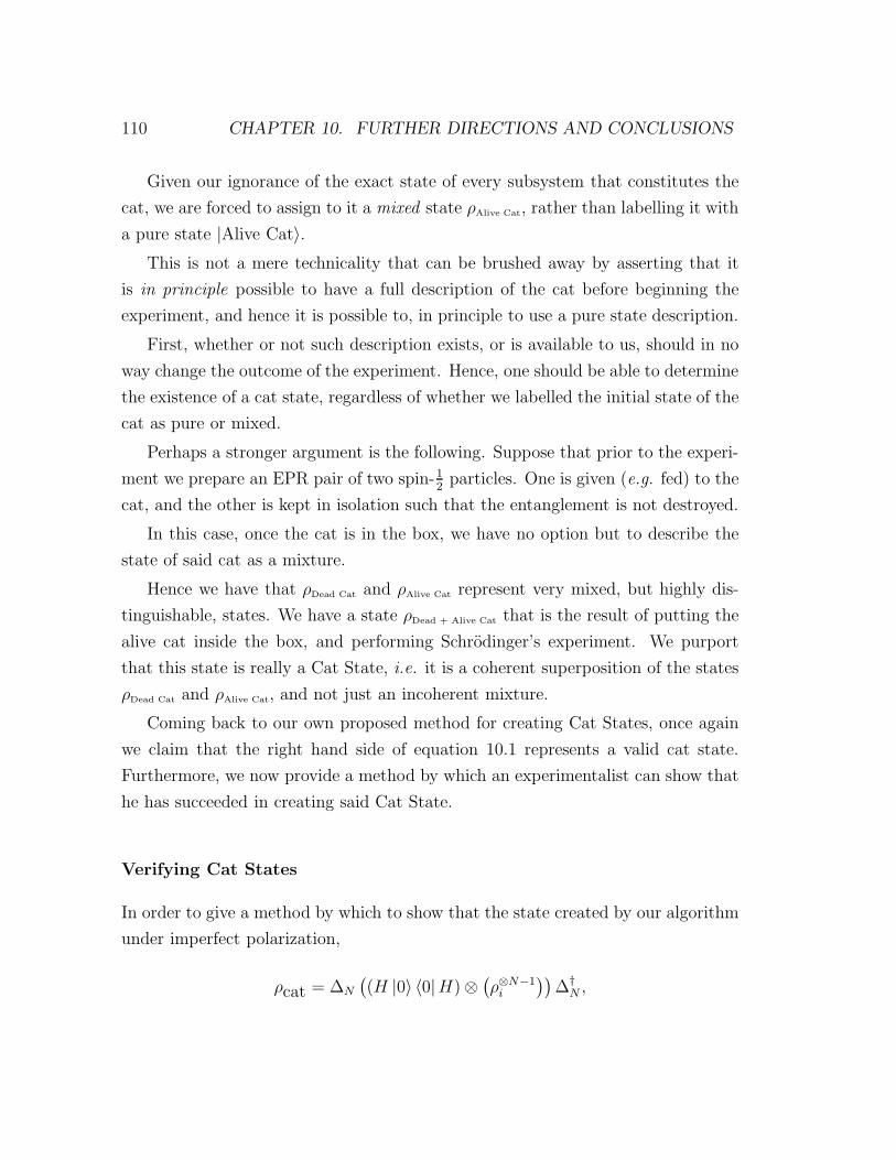
110 CHAPTER 10. FURTHER DIRECTIONS AND CONCLUSIONS
Given our ignorance of the exact state of every subsystem that constitutes the
cat, we are forced to assign to it a mixed state ρAlive Cat, rather than labelling it with
a pure state |Alive Cat〉.This is not a mere technicality that can be brushed away by asserting that it
is in principle possible to have a full description of the cat before beginning the
experiment, and hence it is possible to, in principle to use a pure state description.
First, whether or not such description exists, or is available to us, should in no
way change the outcome of the experiment. Hence, one should be able to determine
the existence of a cat state, regardless of whether we labelled the initial state of the
cat as pure or mixed.
Perhaps a stronger argument is the following. Suppose that prior to the experi-
ment we prepare an EPR pair of two spin-12
particles. One is given (e.g. fed) to the
cat, and the other is kept in isolation such that the entanglement is not destroyed.
In this case, once the cat is in the box, we have no option but to describe the
state of said cat as a mixture.
Hence we have that ρDead Cat and ρAlive Cat represent very mixed, but highly dis-
tinguishable, states. We have a state ρDead + Alive Cat that is the result of putting the
alive cat inside the box, and performing Schrodinger’s experiment. We purport
that this state is really a Cat State, i.e. it is a coherent superposition of the states
ρDead Cat and ρAlive Cat, and not just an incoherent mixture.
Coming back to our own proposed method for creating Cat States, once again
we claim that the right hand side of equation 10.1 represents a valid cat state.
Furthermore, we now provide a method by which an experimentalist can show that
he has succeeded in creating said Cat State.
Verifying Cat States
In order to give a method by which to show that the state created by our algorithm
under imperfect polarization,
ρcat = ∆N
((H |0〉 〈0|H) ⊗
(ρ⊗N−1
i
))Ơ
N ,
10.3. MODIFICATIONS AND FURTHER APPLICATIONS OF
SPIN-AMPLIFICATION 111
is indeed a Cat State and not merely an incoherent mixture, we will follow Leggett
[Leg02]. A, possibly macroscopic, system is in a superposition of two states, as
opposed to a classical mixture of such, if it is possible to induce a interference effect
on said state.
The way to induce such an interference effect is simple. Assuming perfect quan-
tum control, even under the assumption a dirty ancilla, we have that:
H ⊗ I⊗N−1(∆†
N (ρcat) ∆N
)H ⊗ I⊗N−1 = |0〉 〈0| ⊗ ρ⊗N−1
i
Therefore, a method for creating, and verifying a Cat State of consisting of N
spins in the laboratory would be the following:
1. Verify that
∆N
(|0〉 〈0| ⊗
(ρ⊗N
i
))Ơ
N = |0〉 〈0| ⊗ (N)0 ,
and,
∆N
((X |0〉 〈0|X) ⊗
(ρ⊗N
i
))Ơ
N = |1〉 〈1| ⊗ (N)1
where (N)0 and
(N)1 are macroscopically distinguishable. This can be done by
initializing the control qubit appropriately, running the single-spin measure-
ment algorithm as defined earlier and verifying that both outcomes produce
significantly different magnetic field. If the measurement algorithm described
in Chapter 9 has been successfully implemented, this step can easily be done.
2. (a) Create the state
ρcat = ∆N
((H |0〉 〈0|H) ⊗
(ρ⊗N−1
i
))Ơ
N
(b) Verify that the state ρcat is indeed a Cat State by first applying the
transformation
ρresult = H ⊗ I⊗N−1(∆†
N (ρcat)∆N
)H ⊗ I⊗N−1
112 CHAPTER 10. FURTHER DIRECTIONS AND CONCLUSIONS
and then applying the single-spin measurement procedure to verify that
trancilla(ρresult
)= |0〉 〈0|
This procedure could, in theory, generate cat states involving up to N spins,
using O(
3√N)
steps (see Chapter 9 for a discussion of the scaling).
There are a few of caveats. First, we have been assuming perfect quantum
control. This assumption may be relaxed. This relaxation might not be as negative
as one might at first assume. If we use the right error model, we might be able to
predict, and experimentally obtain, an interference effect
Normally, mathematicians assume uncorrelated random errors. This is because
these are the easiest to model. However, in practice, errors in quantum control
seldom behave this way.
Suppose the error in gates behaves in following way. A NOT gate is imple-
mented with a faulty π-pulse which instead of applying the rotation e−iπσx , applies
the transformation e−i(π−ǫ)σx . Recall that applying rotations about the z axis is—for
all practical purposes—error free, since it requires one to simply update the lab-
oratory reference frame with regards to the rotating reference frame of the spins.
Note that.
σze−i(π−ǫ)σxσze
−i(π−ǫ)σx |ψ〉 = |ψ〉 ,
for all possible |ψ〉 and all values of ǫ.
With this in mind, it may be possible to implement ƠN in such a way that
∆†N∆N ≈ 1l even with faulty gates.
Another concern that must be addressed is that, unlike simple spin-measurement,
when implementing the spin amplification algorithm for purposes of generating and
verifying cat states, this procedure must be run in under the phase decoherence, t2,
times.
A question of more theoretical importance is how to quantify the Cat state
created by such a procedure. Currently, all measures of Cat state size contemplate
only pure states [DSC02,MAv06,KWDC07].
It should be possible to formalize some of the intuitive ideas discussed in this
10.4. FURTHER SIMULATIONS OF PHYSICAL SYSTEMS 113
section into an actual measure of Cat size.
10.4 Further Simulations of Physical Systems
In Chapter 7 we studied some physical systems that can be simulated on a QCA. A
natural question to ask, is what other examples of physical systems can be simulated
efficiently, i.e. with at most a polynomial overhead.
For instance, we saw that it is possible to simulate a freely-moving particle. An
interesting extension would be to simulate this same particle, but now subject to
some energy potential, or perhaps a gradient field. This should not be a difficult
extension of the simulation presented in Chapter 7. One would initialize the QCA
so that each cell begins with the value of the strength of the field, direction, etc.
at that point in space. The QCA update rule would then have to be modified to
take into account this field value when moving the particle.
Other interesting examples would be to simulate larger molecules, and how
the atoms within interact with one another. Potentially, this could be useful in
studying, inter alia, how proteins fold. In this case, however, it seems that more
difficult than performing the simulation itself, is getting useful information out of
measurements on the QCA system.
Another interesting avenue is the simulation capabilities of dissipitative QCA.
For example, we know that the continuous limit of a quantum walk gives the
Schrodinger equation for a freely moving particle [BT98]. On the other hand, the
continuous limit of a completely classical random walk closely resembles electric
current [Tet91].
A conjecture put forth in this thesis is that given a quantum walk QCA, with
some appropriate amount of decoherence, and taking its continuous limit, would
give rise to a master equation for a particle subject to an external force. It should be
possible, in principle, to obtain master equations for many actual physical systems
by first positing an appropriate dissipitative QCA, and taking its continuous limit.
If we adhere to the belief that all systems ultimately behave according to some
local quantum rules, then there is no theoretical limit on the type of systems that
114 CHAPTER 10. FURTHER DIRECTIONS AND CONCLUSIONS
can be simulated on QCA.
It is even conceivable that a theoretical framework built around QCA could be
used to model the Universe as a whole.
10.4.1 The Universe as a QCA
The idea of a QCA model of the universe is quite attractive, even if the obstacles
against it are many and large.
A great difficulty would be to make QCA theory work with general relativity.
An obstacle for this, inter alia, is Lorentz invariance.
For instance, take the same quantum walk QCA that we described in Chapter
7. If restricted to one dimension, it is possible to take the continuous limit of this
walk and obtain the relativistic Dirac equation for a single moving particle in free
space [LB05,Mey96a].
Unfortunately, this construction cannot be made to work with Lorentz invari-
ance for QCA with dimension strictly higher than one [Mey96a]. The issue, in
particular, has to do with the evolution not being invariant under rotation of the
reference frame, due to the discrete nature of the lattice.
This is an issue that has been discussed and addressed in quantum cosmological—
quantum gravity—models. For instance, in loop quantum gravity a QCA-like lattice
is put forth as the underlying structure of space-time. However, to make the model
Lorentz invariant, the lattice points are randomly scattered.
While it may be possible to make a QCA model Lorentz invariant another pos-
sible avenue is to forgo perfect Lorentz invariance altogether. It is entirely possible
that Lorentz invariance is a result of a possibly false assumption of continuous
space-time structures.
In particular, a fundamental Lorentz invariant usually taken for granted is ro-
tation of the spatial co-ordinates.
If one were to give up on rotational invariance as a fundamental principle and
embrace a QCA type formalism as the underlying structure of space-time it is
possible that this would lead to a ‘third’ quantization.
10.5. CLOSING REMARKS 115
In order to better visualize what is meant by third quantization, consider a
qubit:
α |0〉 + e−iθβ |1〉 .
Suppose this qubit represents a spin-12
system. Generally, the parameters α, β
and θ are considered to be real-valued. Note that these parameters are with respect
to a certain eigenbasis, given by some observable. Let us call this observable σz .
Fix α and β. For every value of θ there is an observable σθ such that the
superposition given above is the plus one eigenstate of said observable. In principle,
there exists an experimental setup to measure σθ for any real value θ. This is
consistent with the notion of continuous space.
Now, let us suppose that space is not continuous, but rather is a discrete lat-
tice. Then there would be no freedom to choose from a continuum of observables.
Likewise, this would postulate that the state of the qubit above must in fact be
written as
αk |0〉 + e−iθk/2βk |1〉 ,
where k is some, heretofore undetermined, universal constant. Intuitively, what this
says for the case of a spin-12
system, is that there is a minimum quanta of rotation
about any axis. This constant could, in principle, be derived from the QCA lattice
structure, and experimentally verified.
10.5 Closing Remarks
In this thesis, we have presented a model of quantum cellular automata based
on local unitary operators. We have shown that it has distinct advantages over
previous cellular automata quantizations. In particular, we have shown that given
any LUQCA it is always possible to give an efficient, low-depth quantum circuit that
faithfully represents it. This leads to the conclusion that any universal quantum
computer could implement an LUQCA efficiently.
More importantly, however, we have also shown that it is possible to implement
LUQCA in experimental setups that are arguably simpler than traditional quantum
116 CHAPTER 10. FURTHER DIRECTIONS AND CONCLUSIONS
circuit based algorithms: for instance, globally addressing spins in NMR or ESR. At
the same time, we have shown that our model is universal for quantum computation.
We gave an explicit proof of an efficient simulation of quantum circuits using a two-
dimensional QCA. We also presented a proof of universality for one-dimensional
LUQCA.
Furthermore, we showcased the LUQCA as a modelling and simulation tool.
We gave explicit constructions within the LUQCA model for simulating certain
spin-chain systems. We also showed how to construct quantum lattice gases within
this model.
Finally, we have shown that QCA in previous models can be efficiently translated
into QCA within the model presented here. For example, a universal QCA in
previous models [Wat95, SFW06] can easily become a universal QCA within the
local unitary model. This fact was used to prove the universality of one-dimensional
LUQCA. All of these facts suggest that the LUQCA is a very strong model.
The purpose of this thesis has been to motivate, develop and showcase a model of
quantum cellular automata based on strictly local, translation-commuting, unitary
operators. It is an author’s conjecture that the construction given here is the most
general of this form.
Perhaps most importantly, we have opened new and interesting avenues of re-
search, from algorithms, to theoretical and experimental physics.
Ultimately, it is the author’s hope that this body of work serves to help unify
the several methods, results, and views surrounding QCA into one single, cohesive
paradigm.
Bibliography
[ANVA+99] M. Arndt, O. Nairz, J. Vos-Andreae, C. Keller, G. van der Zouw, and
A. Zeilinger, “Wave-particle duality of C60 molecules,” Nature, vol.
401, no. 6754, pp. 680–682, 1999.
[BAB+06] S. C. Benjamin, A. Ardavan, G. A. D. Briggs, D. A. Britz, D. Gun-
lycke, J. Jefferson, M. A. G. Jones, D. F. Leigh, B. W. Lovett, A. N.
Khlobystov, S. A. Lyon, J. J. L. Morton, K. Porfyrakis, M. R. Sam-
brook, and A. M. Tyryshkin, “Towards a fullerene-based quantum
computer,” Journal of Physics: Condensed Matter, vol. 18, no. 21,
pp. S867–S883, 2006.
[BB03] S. C. Benjamin and S. Bose, “Quantum computing with an always-on
Heisenberg interaction,” Physical Review Letters, vol. 90, no. 24, p.
247901, Jun 2003.
[BB04] S. C. Benjamin and S. Bose, “Quantum computing in arrays coupled
by “always-on” interactions,” Physical Review A, vol. 70, no. 3, p.
032314, Sep 2004.
[BBK03] A. Bririd, S. C. Benjamin, and A. Kay, “Quantum error correction in
globally controlled arrays,” e-print arXiv.org:quant-ph/0308113, 2003.
[Ben00] S. C. Benjamin, “Schemes for parallel quantum computation without
local control of qubits,” Physical Review A, vol. 61, no. 2, p. 020301
(R), Jan 2000.
117
118 BIBLIOGRAPHY
[Ben04] S. C. Benjamin, “Multi-qubit gates in arrays coupled by ’always-on’
interactions,” New Journal of Physics, vol. 6, p. 61, Jun 2004.
[BLR04] S. C. Benjamin, B. W. Lovett, and J. H. Reina, “Optical quan-
tum computation with perpetually coupled spins,” Physical Review
A, vol. 70, no. 6, p. 060305 (R), Dec 2004.
[Bog98] B. Boghosian, “Simulating quantum mechanics on a quantum com-
puter,” Physica D, vol. 120, pp. 30–42, 1998.
[BT98] B. M. Boghosian and W. Taylor, “Quantum lattice-gas model for the
many-particle schrodinger equation in d dimensions,” Physical Review
E, vol. 57, no. 1, pp. 54–66, Jan 1998.
[BV93] E. Bernstein and U. Vazirani, “Quantum complexity theory,” in Pro-
ceedings of the 25th Annual ACM Symposium on Theory of Comput-
ing, N. Y. ACM Press, Ed., 1993, pp. 11 – 20.
[BV97] E. Bernstein and U. Vazirani, “Quantum complexity theory,” SIAM
Journal on Computing, vol. 26, no. 5, pp. 1411–1473, 1997.
[BW03] G. K. Brennen and J. E. Williams, “Entanglement dynamics in 1d
quantum cellular automata,” Physical Review A, vol. 68, p. 042311,
2003.
[CD98] B. Chopard and M. Droz, Cellular Automata Modeling of Physical
Systems. Cambridge University Press, 1998.
[CEB+05] P. Cappellaro, J. Emerson, N. Boulant, C. Ramanathan, S. Lloyd,
and D. G. Cory, “Entanglement assisted metrology,” Physical Review
Letters, vol. 94, no. 2, p. 020502, Jan 2005.
[CMG90] D. G. Cory, J. B. Miller, and A. N. Garroway, “Time-suspension
multiple-pulse sequences: Applications to solid-state imaging,” Jour-
nal of Magnetic Resonance, vol. 90, pp. 205–213, 1990.
BIBLIOGRAPHY 119
[CS96] A. R. Calderbank and P. W. Shor, “Good quantum error-correcting
codes exist,” Physical Review A, vol. 54, no. 2, pp. 1098–1105, Aug
1996.
[Deu85] D. Deutsch, “Quantum theory, the Church-Turing principle and the
universal quantum computer,” Proceedings of the Royal Society of
London Ser. A, vol. A400, pp. 97–117, 1985.
[DLS97] C. Durr, H. LeThanh, and M. Santha, “A decision procedure for well-
formed linear quantum cellular automata,” Random Structures and
Algorithms, vol. 11, pp. 381–394, 1997.
[DS96] C. Durr and M. Santha, “A decision procedure for unitary linear quan-
tum cellular automata,” in FOCS ’96: Proceedings of the 37th Annual
Symposium on Foundations of Computer Science. Washington, DC,
USA: IEEE Computer Society, 1996, p. 38.
[DSC02] W. Dur, C. Simon, and J. I. Cirac, “On the effective size of certain
“Schrodinger cat” like states,” Physical Review Letters, vol. 89, p.
210402, 2002.
[Fey82] R. Feynman, “Simulating physics with computers,” International
Journal of Theoretical Physics, vol. 21, no. 6&7, pp. 467–488, 1982.
[FKK07] D. M. Forrester, K. E. Kurten, and F. V. Kusmartsev, “Magnetic
cellular automata and the formation of glassy and magnetic structures
from a chain of magnetic particles,” Physical Review B, vol. 75, no. 1,
p. 014416, Jan 2007.
[FT06] J. Fitzsimons and J. Twamley, “Globally controlled quantum wires for
perfect qubit transport, mirroring, and computing,” Physical Review
Letters, vol. 97, no. 9, p. 090502, Sep 2006.
[FT07] J. Fitzsimons and J. Twamley, “Globally controlled fault tolerant
quantum computation,” e-print arXiv:0707.1119v1, 2007.
120 BIBLIOGRAPHY
[FXBJ07] J. Fitzsimons, L. Xiao, S. C. Benjamin, and J. A. Jones, “Quantum
information processing with delocalized qubits under global control,”
Physical Review Letters, vol. 99, no. 3, p. 030501, 2007.
[Gac83] P. Gacs, “Reliable computation with cellular automata,” in Proceed-
ings of the 15th Annual ACM Symposium on Theory of Computing
(STOC), 1983, pp. 32–41.
[Got98] D. Gottesman, “Theory of fault-tolerant quantum computation,”
Physical Review A, vol. 57, no. 1, pp. 127–137, Jan 1998.
[Got07] D. Gottesman, “Fault-tolerant quantum computation,” e-print
arXiv:quant-ph/0701112, 2007.
[ICJ+06] A. Imre, G. Csaba, L. Ji, A. Orlov, G. H. Bernstein, and W. Porod,
“Majority logic gate for magnetic quantum-dot cellular automata,”
Science, vol. 311, no. 5758, pp. 205–208, Jan 2006.
[Kan98] B. E. Kane, “A silicon-based nuclear spin quantum computer,” Nature,
vol. 393, no. 6681, pp. 133–137, May 1998.
[Kay05] A. Kay, “Error correcting the control unit in global control schemes,”
e-print arXiv:quant-ph/0504197, 2005.
[Kay07a] A. Kay, “Deriving a fault-tolerant threshold for a global control
scheme,” e-print arXiv:quant-ph/0702239, 2007.
[Kay07b] P. Kaye, “Cooling algorithms based on the 3-bit majority,” e-print
arXiv:quant-ph/0703194, 2007.
[KBST05] M. Khatun, T. Barclay, I. Sturzu, and P. D. Tougaw, “Fault toler-
ance calculations for clocked quantum-dot cellular automata devices,”
Journal Of Applied Physics, vol. 98, no. 9, p. 094904, Nov 2005.
[KBST06] M. Khatun, T. Barclay, I. Sturzu, and P. D. Tougaw, “Fault toler-
ance properties in quantum-dot cellular automata devices,” Journal
BIBLIOGRAPHY 121
Of Physics D: Applied Physics, vol. 39, no. 8, pp. 1489–1494, Apr
2006.
[KWDC07] J. I. Korsbakken, K. B. Whaley, J. DuBois, and J. I. Cirac, “A
measurement-based measure of the size of macroscopic quantum su-
perpositions,” Physical Review A, vol. 75, p. 042106, 2007.
[LB05] P. J. Love and B. M. Boghosian, “From Dirac to diffusion: Deco-
herence in quantum lattice gases,” Quantum Information Processing,
vol. 4, no. 4, pp. 335–354, Oct 2005.
[LB06] P. J. Love and B. Boghosian, “Type-II quantum algorithms,” Physica
A, vol. 362, pp. 210–214, 2006.
[LBM04] P. J. Love, B. Boghosian, and D. A. Meyer, “Lattice-gas simulations
of dynamical geometry in one-dimension,” Philosophical Transactions
of the Royal Society, vol. 362, pp. 1667–1675, 2004.
[Leg02] A. J. Leggett, “Testing the limits of quantum mechanics: motiva-
tion, state of play, prospects,” Journal of Physics: Condensed Matter,
vol. 14, no. 15, pp. R415–R451, 2002.
[LK05] J.-S. Lee and A. K. Khitrin, “Stimulated wave of polarization in a
one-dimensional ising chain,” Physical Review A, vol. 71, no. 6, p.
062338, Jun 2005.
[Llo93] S. Lloyd, “A potentially realizable quantum computer,” Science, vol.
261, pp. 1569–1571, 1993.
[LTPB93] C. S. Lent, P. D. Tougaw, W. Porod, and G. H. Bernstein, “Quantum
cellular automata,” Nanotechnology, vol. 4, no. 1, pp. 49–57, 1993.
[MAv06] F. Marquardt, B. Abel, and J. von Delft, “Measuring the size of a
schroedinger cat state,” e-print arXiv:quant-ph/0609007, 2006.
122 BIBLIOGRAPHY
[Mey96a] D. A. Meyer, “From quantum cellular automata to quantum lattice
gases,” Journal of Statistical Physics, vol. 85, pp. 551–574, 1996.
[Mey96b] D. A. Meyer, “On the absence of homogeneous scalar unitary cellular
automata,” Physics Letters A, vol. 223, no. 5, pp. 337–340, 1996.
[MSPB03] W. Marshall, C. Simon, R. Penrose, and D. Bouwmeester, “Towards
quantum superpositions of a mirror,” Physical Review Letters, vol. 91,
p. 130401, 2003.
[OMH87] K. Obermayer, G. Mahler, and H. Haken, “Multistable quantum sys-
tems: Information processing at microscopic levels,” Physical Review
Letters, vol. 58, no. 17, pp. 1792–1795, Apr 1987.
[OTM88] K. Obermayer, W. G. Teich, and G. Mahler, “Structural basis of mul-
tistationary quantum systems. i. effective single-particle dynamics,”
Physical Review B, vol. 37, no. 14, pp. 8096–8110, May 1988.
[PDC05] C. A. Perez-Delgado and D. Cheung, “Models of quantum cellular
automata,” e-print arXiv:quant-ph/0508164, 2005.
[PDC07] C. A. Perez-Delgado and D. Cheung, “Local unitary quantum cellular
automata,” Physical Review A, vol. 76, no. 3, p. 032320, 2007.
[PDCM+06] C. A. Perez-Delgado, D. Cheung, M. Mosca, P. Cappellaro, and
D. Cory, “Quantum cellular automata and single spin measurement,”
in Proceedings of the Asian Conference on Quantum Information Sci-
ence (AQIS ’06). Beijing, China: Key Laboratory of Quantum In-
formation, Chinese Academy of Science, 2006.
[PDMCC06] C. A. Perez-Delgado, M. Mosca, P. Cappellaro, and D. G. Cory, “Sin-
gle spin measurement using cellular automata techniques,” Physical
Review Letters, vol. 97, no. 10, p. 100501, 2006.
[Rau05] R. Raussendorf, “Quantum cellular automaton for universal quantum
computation,” Physical Review A, vol. 72, no. 2, p. 022301, Aug 2005.
BIBLIOGRAPHY 123
[Sch35] E. Schrodinger, “Die gegenwartige situation in der quantenmechanik,”
Naturwissenschaften, vol. 23, no. 48, pp. 807–812, 1935.
[SFW06] D. J. Shepherd, T. Franz, and R. F. Werner, “Universally pro-
grammable quantum cellular automaton,” Physical Review Letters,
vol. 97, no. 2, p. 020502, Jul 2006.
[Sin06] S. Sinha, “Coherent control of dipolar coupled spins in large hilbert
spaces,” Ph.D. dissertation, Massachusetts Institute of Technology,
2006.
[SMW05] L. J. Schulman, T. Mor, and Y. Weinstein, “Physical limits of heat-
bath algorithmic cooling,” Physical Review Letters, vol. 94, no. 12, p.
120501, 2005.
[SMW07] L. J. Schulman, T. Mor, and Y. Weinstein, “Physical limits of heat-
bath algorithmic cooling,” SIAM Journal on Computing, vol. 36, no. 6,
pp. 1729–1747, 2007.
[STD05] K. M. Svore, B. M. Terhal, and D. P. DiVincenzo, “Local fault-tolerant
quantum computation,” Physical Review A, vol. 72, no. 2, p. 022317,
2005.
[SV99] L. J. Schulman and U. V. Vazirani, “Molecular scale heat engines and
scalable quantum computation,” in Proceedings 31’st ACM Sympo-
sium on Theory of Computing, (STOC99), Atlanta, GA, 1999, pp.
322–329.
[SW04] B. Schumacher and R. F. Werner, “Reversible quantum cellular au-
tomata,” e-print arXiv:quant-ph/0405174, 2004.
[Tet91] P. Tetali, “Random walks and the effective resistance of networks,”
Journal of Theoretical Probability, vol. 4, no. 1, pp. 101–109, 1991.
[Thi83] W. Thirring, Quantum Mechanics of Large Systems, A Course in
Mathematical Physics. New York: Springer-Verlag, 1983, vol. 4.
124 BIBLIOGRAPHY
[TM87] T. Toffoli and N. Margolus, Cellular Automata Machines. MIT Press,
1987.
[Tof77] T. Toffoli, “Cellular automata mechanics,” Ph.D. dissertation, The
University of Michigan, 1977.
[VC06] K. G. H. Vollbrecht and J. I. Cirac, “Reversible universal quantum
computation within translation-invariant systems,” Physical Review
A, vol. 73, no. 1, p. 012324, Jan 2006.
[vD96] W. van Dam, “Quantum cellular automata,” Master’s thesis, Univer-
sity of Nijmegen, 1996.
[vN51] J. von Neumann, “The general and logical theory of automata,” in
Cerebral Mechanisms in Behavior. John Wiley and Sons, 1951, pp.
1–41.
[vN66] J. von Neumann, Theory of Self-Reproducing Automata. Urbana,
Illinois: University of Illinois Press, 1966.
[Wat95] J. Watrous, “On one-dimensional quantum cellular automata,” in
FOCS ’95: Proceedings of the 36th Annual Symposium on Founda-
tions of Computer Science (FOCS’95). Washington, DC, USA: IEEE
Computer Society, 1995, p. 528.
[Wau98] J. S. Waugh, “Equilibrium and ergodicity in small spin systems,”
Molecular Physics, vol. 95, no. 5, pp. 731–735, Dec 1998.
[WJ06] K. Walus and G. A. Jullien, “Design tools for an emerging soc tech-
nology: Quantum-dot cellular automata,” Proceedings Of The IEEE,
vol. 94, no. 6, pp. 1225–1244, Jun 2006.
[Wol83] S. Wolfram, “Statistical mechanics of cellular automata,” Reviews of
Modern Physics, vol. 55, pp. 601–644, Jul. 1983.
[Wol02] S. Wolfram, A New Kind of Science. Wolfram Media, 2002.
BIBLIOGRAPHY 125
[Yao93] A. Yao, “Quantum circuit complexity,” in Proceedings of the 34th An-
nual Symposium on Foundations of Computer Science. Los Alamitos,
CA: Institute of Electrical and Electronic Engineers Computer Society
Press, 1993, pp. 352–361.
[Yep98] J. Yepez, “Quantum computation of fluid dynamics,” in QCQC ’98:
Selected papers from the First NASA International Conference on
Quantum Computing and Quantum Communications. London, UK:
Springer-Verlag, 1998, pp. 34–60.